symmetry group methods for fundamental solutions

J. Differential Equations 207 (2004) 285 – 302

www.elsevier.com/locate/jde

Symmetry group methods for fundamentalsolutions

Mark Craddock∗, Eckhard PlatenDepartment of Mathematical Sciences, University of Technology Sydney, P.O. Box 123, Broadway, New

South Wales 2007, Australia

Received 10 October 2003; revised 18 May 2004

Available online 11 September 2004

Abstract

This paper uses Lie symmetry group methods to study PDEs of the formut=xuxx+f (x)ux.We show that when the drift functionf is a solution of a family of Ricatti equations, thensymmetry techniques can be used to find a fundamental solution.© 2004 Elsevier Inc. All rights reserved.

Keywords:Lie symmetry groups; Fundamental solutions; Characteristic solutions; Transition densities

1. Introduction

The purpose of this paper is to use symmetry group methods to compute fundamentalsolutions for a class of partial differential equations (PDEs), of the form,

ut = xuxx + f (x)ux, x�0. (1.1)

By a fundamental solution, we mean a kernel functionp(t, x, y) such thatu(x, t) =∫∞0 �(y)p(t, x, y) dy is a solution of the Cauchy problem for (1.1) with u(x,0) =

�(x).

∗ Corresponding author.E-mail address:[email protected](M. Craddock).

0022-0396/$ - see front matter © 2004 Elsevier Inc. All rights reserved.doi:10.1016/j.jde.2004.07.026

http://www.elsevier.com/locate/jde

mailto:[email protected]

286 M. Craddock, E. Platen / J. Differential Equations 207 (2004) 285–302

We will show that such a fundamental solution can often be obtained by Lie sym-metry group methods when the drift functionf is a solution of one of the followingthree families of Ricatti equations:

xf ′ − f + 12 f

2 = Ax + B, (1.2)

xf ′ − f + 12 f

2 = Ax2 + Bx + C, (1.3)

xf ′ − f + 12 f

2 = Ax 32 + Bx2 + Cx − 3

8, (1.4)

whereA,B andC are arbitrary constants.The problem of computing fundamental solutions for PDEs of the form (1.1), arises

in the study of one-dimensionalgeneralized square rootor GSR processes. LetX ={Xt, t ∈ [0, T ]} satisfy the Itô stochastic differential equation (SDE),

dXt = f (Xt ) dt +√

2Xt dWt (1.5)

for t ∈ [0, T ]. HereW is a standard Wiener process, andf is a drift function. It is wellknown that the transition density,p(t, x, y) for X, is given by the fundamental solutionof the PDE (1.1). See for example Revuz and Yor[16].

GSR processes have applications in finance and other areas. Certain GSR processesexhibit a property known as mean reversion, making them ideal for modelling interestrates. For example, the GSR process with drift equal tof (x) = a − bx is used byCox, Ingersoll and Ross (CIR) to model bond prices. (See the book[8]). Longstaff bycontrast, models bond prices with a GSR process in which the driftf (x) = a − b√x.(See[12] for Longstaff’s analysis and a comparison with the CIR model). The transitiondensities for both the CIR model and the Longstaff model can be obtained by ourmethods.

Another application of GSR processes is to the modelling of inflation rates. Typicallya central bank would like to keep inflation within a certain band, say(�,�). Suchinflation rates can be modelled by GSR processes in which the drift has discontinuitiesat x = �, x = �. An instance of such a process is given by our Example 4.8. GSRprocesses also play a fundamental role in theminimum market modelof Platen,[15],which models equity and currency markets. In our Example 4.2, we present a simpleapplication of our methods to the pricing of an option on a commodity.

2. Symmetry methods and fundamental solutions

Symmetry group methods provide a natural approach to the problem of findingfundamental solutions of PDEs. The book by Olver[14] gives an excellent modernaccount of Lie’s theory of symmetry groups. See also the books by Miller[13] andBluman and Kumei[1] and the papers[2–4]. Lie himself considered symmetries ofhigher order PDEs in[9,10]. The book[11] is based on Lie’s papers.

M. Craddock, E. Platen / J. Differential Equations 207 (2004) 285–302 287

For illustration, consider the one-dimensional heat equation. Lie showed that ifu(x, t)

is a solution of the equationuxx = ut , then so is

u�(x, t) = 1√1 + 4�t

exp

{ −�x2

1 + 4�t

}u

(x

1 + 4�t,

t

1 + 4�t

)(2.1)

for � sufficiently small (see for example[14]). In (2.1), let u = 1, t → t − 14 �, and set

� = �. In this way, we obtain the fundamental solution of the heat equation,k(x, t) =1√4�te− x2

4t , from the constant solution,u = 1, by simple group transformation.It is natural to ask whether we can obtain fundamental solutions for other PDEs by

similar means? In a recent paper, Craddock and Dooley[5] showed that for the heatequation on a nilpotent Lie group, there is always a symmetry which maps the constantsolution to the fundamental solution. They also studied the equation

ut = uxx + f (x)ux. (2.2)

The fundamental solution of (2.2) can be obtained from the solutionu = 1 by asymmetry transformation, whenever the drift functionf is a solution of any one of fivefamilies of Ricatti equations. This immediately leads to a rich class of PDEs, whosefundamental solutions can be explicitly computed. It also motivates the remainder ofthis paper.

In the current work, our approach is to obtain an integral transform of the fundamentalsolution by a symmetry transformation. In Section 4, we show that if the drift functionf satisfies (1.2), then we can obtain the solution

U�(x, t) =∫ ∞

0e−�yp(t, x, y) dy, (2.3)

of (1.1) from the trivial solutionu = 1 by symmetry. This is the Laplace transformof p(t, x, y). So the fundamental solution can then be recovered by taking the inverseLaplace transform ofU�. We shall callU� a characteristic solutionfor (1.1).

In Section 5, we treat the case whenf is a solution of (1.3). Here, we do notimmediately obtain a characteristic solution. Rather, we obtain an integral transform ofthe fundamental solution which is more complicated. However, this typically reducesto a Laplace transform. We will present some illustrative examples.

In Section 6, we treat the case whenf satisfies (1.4). For the subcase, whenB = 0, weare again able to derive a characteristic solution from a trivial solution by a symmetrytransformation. Iff satisfies (1.4) with B �= 0, we can also obtain an integral transformof p(t, x, y).

Our techniques lead to a rich class of PDEs with explicitly computable fundamentalsolutions. Many of the fundamental solutions that our methods give appear to be new.We also recover all the well-known examples, such as when the drift functionf isaffine.


The method that we describe in this paper is one of two symmetry-based techniqueswhich allow us to construct fundamental solutions for these partial differential equations.In a subsequent paper, we shall describe a second approach. This method yields entirelynew fundamental solutions.

3. The infinitesimal symmetries

In this section, we present a complete list ofall possible Lie symmetry algebras forPDEs of the form (1.1). Recall that if the vector field

v = �(x, t, u)��x

+ �(x, t, u)��t

+ (x, t, u)��u, (3.1)

generates a symmetry of (1.1), thenv must satisfy Lie’s condition:

pr2 v[ut − xuxx − f (x)ux] = 0, wheneverut = xuxx + f (x)ux.

Here pr2 v denotes the second prolongation ofv. If v generates a symmetry of (1.1),then standard symmetry group calculations lead to the following conditions on thecoefficients�, � and . The full details are given in[6]. Let �(x, t) be an arbitrarysolution of (1.1). Then

� = x�t +√x(t), (x, t, u) = �(x, t)u+ �(x, t),

� = −1

2x�t t − √

xt +1

2√x

(1

2− f (x)

) − 1

2f (x)�t + �(t)

for some functions and �. Now the function � depends only ont. Set Lf =xf ′ − f + 1

2 f2. Then

−1

2x�t t t − √

xt t + �t = −1

2

d

dx

(Lf

)�t +

[3 + 8Lf − 8x d

dx(Lf )

16x32

].

These equations fix�, �,,� and for everyC2 drift function f.We now list the infinitesimal point symmetries of (1.1). In the following, we set

g(x) = 12√x

(12 − f (x)) . As usual, we write�u for �

�u etc.

Case1: Let xf ′ − f + 12 f

2 = Ax + B, whereA andB are constants.Subcase1a: If 3+ 8B = 0, then a basis for the Lie algebra is:

v� = �(x, t)�u, v1 = √x�x − g(x)u�u, v2 = �t , v3 = u�u,

v4 = 2x�x + 2t�t − (f (x)+ At)u�u, v5 = √xt�x − (√x − g(x)t)u�u,

v6 = 8xt�x + 4t2�t − (4x + 4f (x)t + 2At2)u�u.


Subcase1b: If 3+ 8B �= 0, then the Lie algebra is spanned by the vector fields{v�, v2, v3, v4, v6}, from Subcase 1a.


2 = 12Ax

2 + Bx + C, whereA,B and C are constants.The extra 1

2 in the coefficient ofx2 is convenient here.Subcase2a: If A > 0, and 3+ 8C = 0, a basis for the Lie algebra is:

v� = �(x, t)�u v1 = √xe

12

√At�x − 1

2

(√Ax − 2g(x)

)e

12

√Atu�u, v2 = �t ,

v3 = u�u, v4 = x√Ae√At�x + e

√At�t − 1

2(Ax + √

Af (x)+ B)e√Atu�u,

v5 = √xe−

12

√At�x + 1

2

(√Ax + 2g(x)

)e−

12

√Atu�u,

v6 = −x√Ae−√At�x + e−

√At�t − 1

2(Ax − √

Af (x)+ B)e−√Atu�u.

Subcase2b: If 3+ 8C �= 0, then the Lie algebra is spanned by the vector fields{v�, v2, v3, v4, v6}, from the list in Subcase 2a.Subcase2c: If A < 0, then a basis for the Lie algebra of symmetries may beobtained from the real and imaginary parts of the vector fields in Subcases 2aand 2b.


2 = Ax 32 + Bx2 + Cx +D. If 3 + 8D �= 0, then the Lie

algebra of symmetries is spanned byv� = ��u, v1 = �t , andv2 = u�u. If 3 +8D = 0,there are three subcases.

Subcase3a: If B = 0, then a basis for the Lie algebra consists ofv� = �(x, t)�uand

v1 = √x�x −

(At

6− g(x)

)u�u, v2 = �t , v4 =

(2x + A

2

√xt2)

�x

+2t�t −((C + A√

x)t + A2

36t3 − A

2g(x)t2 + f (x)

)u�u, v3 = u�u,

V5 = t√x�x −

(A

12t2 + √

x − g(x)t)u�u, v6 =

(8xt + 2A

3

√xt3)

�x

+4t2�t −(

4x + 2Ct2 + 4f (x)t + A2

36t4 + 2A

√xt2 − 2

3Ag(x)t3

)u�u.

Subcase3b: If B > 0, set � = 2A3√B

and = 2A2+9BC18B . Then a basis consists of

v� = �(x, t)�u and

v1 = √xe

12

√Bt�x −

(1

2

√B

√x − g(x)+ �

2

)e

12

√Btu�u,


v2 = √xe−

12

√Bt�x +

(1

2

√B

√x + g(x)+ �

2

)e−

12

√Btu�u,

v3 = u�u, v4 = �t , v5 =(�√x + √

Bx)e√Bt�x + e

√Bt�t

−(B

2x + 2A

3

√x +

√B

2f (x)− �

2g(x)+

)e√Btu�u,

v6 = −(�√x + √

Bx)e−

√Bt�x + e−

√Bt�t

−(B

2x + 2A

3

√x −

√B

2f (x)+ 1

2�g(x)+

)e−

√Btu�u.

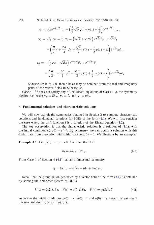
Subcase3c: If B < 0, then a basis may be obtained from the real and imaginaryparts of the vector fields in Subcase 3b.

Case4: If f does not satisfy any of the Ricatti equations of Cases 1–3, the symmetryalgebra has basis:v� = ��u, v1 = �t and v2 = u�u.

4. Fundamental solutions and characteristic solutions

We will now exploit the symmetries obtained in Section 3 to compute characteristicsolutions and fundamental solutions for PDEs of the form (1.1). We will first considerthe case where the drift functionf is a solution of the Ricatti equation (1.2).

The key observation is that the characteristic solution is a solution of (1.1), withthe initial conditionu(x,0) = e−�x. By symmetry, we can obtain a solution with thisinitial data from a solution with initial datau(x,0) = 1. We illustrate by an example.

Example 4.1. Let f (x) = �, � > 0. Consider the PDE

ut = xuxx + �ux. (4.1)

From Case 1 of Section 4 (4.1) has an infinitesimal symmetry

v6 = 8xt�x + 4t2�t − (4x + 4�t)u�u.

Recall that the group action generated by a vector field of the form (3.1), is obtainedby solving the first-order system of ODEs,

x′(�) = �(x, t , u), t ′(�) = �(u, t , u), u′(�) = (x, t , u) (4.2)

subject to the initial conditionsx(0) = x, t(0) = t and u(0) = u. From this we obtainthe new solution,u�(x, t) = u(x, t ).


Solving these equations forv6, gives

u�(x, t) = 1

(1 + 4�t)�exp

{ −4�x1 + 4�t

}u

(x

(1 + 4�t)2,

t

1 + 4�t

). (4.3)

Thus if u is any solution of (4.1), then (4.3) is also a solution, at least for� sufficientlysmall. We set� = 4�, and takeu = 1. By symmetry,

U�(x, t) = 1

(1 + �t)�exp

{ −�x1 + �t

}, (4.4)

is also a solution of (4.1). This is known to be a characteristic solution of (4.1). Toinvert it, let L denote Laplace transformation in�. Then

L−1(

1

�� ek�

)=(yk

) �−12I�−1(2

√ky), � > 0, (4.5)

whereI� is a modified Bessel function of the first kind with order�.Elementary properties of Laplace transforms and (4.5) now give,

p(t, x, y) = L−1(

1

(1 + �t)�exp

{ −�x1 + �t

})

= 1

t

(x

y

) 1−�2

I�−1

(2√xy

t

)exp

{− (x + y)

t

}. (4.6)

This is the fundamental solution of (4.1) given in [16].

This example shows that it is sometimes possible to obtain a characteristic solutionof (1.1) by a symmetry transformation. In fact, we can easily establish the followingtheorem.

Theorem 4.1. Let f be a solution of the Ricatti equation

xf ′ − f + 12 f

2 = Ax + B. (4.7)

Let

U�(x, t) = exp

{−�(x + 1

2At2)

1 + �t− 1

2

(F(x)− F

(x

(1 + �t)2

))}, (4.8)


whereF ′(x) = f (x)/x and ��0. ThenU� is a characteristic solution of(1.1). Thatis, U� is the Laplace transform of the fundamental solutionp(t, x, y) of (1.1).

Proof. Clearly U�(x,0) = e−�x. Sincexf ′ − f + 12 f

2 = Ax + B, then, from Case 1of Section 3, Eq. (1.1) has an infinitesimal symmetry of the formv6 = 8xt�x+4t2�t −(4x + 4f (x)t + 2At2

)u�u.

Exponentiatingv6, we see that ifu is a solution of (1.1), then so is

u�(x, t) = exp

{− (4�x + 2A�t2)

1 + 4�t− 1

2

(F(x)− F

(x

(1 + 4�t)2

))}

×u(

x

(1 + 4�t)2,

t

1 + 4�t

),

where F ′(x) = f (x)/x. Taking u = 1, and setting� = 4�, we see that (4.8) is asolution of (1.1) for all ��0.

First, let us assume thatU� is a Laplace transform. Now define(y) = ∫∞0 (�)

e−�y d�, where is a distribution with the property that∫∞

0 (�)U�(x, t) d� is abso-lutely convergent. Differentiation under the integral sign shows thatu(x, t) = ∫∞

0 (�)U�(x, t) d� is a solution of (1.1) with u(x,0) = (x). Now let p(t, x, y) be the inverseLaplace transform ofU�. Then by Fubini’s theorem

∫ ∞

0(y)p(t, x, y) dy =

∫ ∞

0

(∫ ∞

0(�)e−�yp(t, x, y) d�

)dy

=∫ ∞

0(�)

(∫ ∞

0e−�yp(t, x, y) dy

)d�

=∫ ∞

0(�)U�(x, t) d� = u(x, t).

Henceu(x, t) = ∫∞0 (y)p(t, x, y) andu(x,0) = (x). Next, observe that

∫∞0 p(t, x, y)

= U0(x, t) = 1, as expected. Consequently,p(t, x, y) is a fundamental solution of(1.1).

Now, we prove thatU�(x, t) is the Laplace transform of a generalised functionp(t, x, y). The case whenA = 0 clearly yields a Laplace transform, so we assume thatA �= 0.

It is well known that a functionK(�) is a Laplace transform if it can be written in theform K(�) = G(�)H(�), where bothG andH are Laplace transforms. (See for example

the book by Widder[17]). Now U� is the product of H�(x, t) = exp{

12F

(x

(1+�t)2

)}andG�(x, t) = exp

{−�(x+ 1

2At2)

1+�t − 12F(x)

}. G� is well known to be a Laplace trans-

form. We therefore have to show thatH� is a Laplace transform.


Under the change of variablesf = 2xy′/y, the Ricatti equationxf ′ − f + 12 f

2 =h(x), becomes the second-order linear ODE,

2x2y′′(x)− h(x)y(x) = 0. (4.9)

The general solution of (4.9) for h(x) = Ax + B, is

y(x) = c1x12 I√1+2B

(√2Ax

)+ c2x

12 I−√

1+2B

(√2Ax

). (4.10)

From (4.10), solutions ofxf ′ − f + 12 f

2 = Ax + B, can be obtained. NowF ′(x) =f (x)/x. Hence 1

2 F(x) = ∫y′(x)/y(x) dx = ln y(x). Thus H�(x, t) = y( x

(1+�t)2 ).

By (4.10), H� is a Laplace transform if√x

1+�t I±√1+2B(

√2Ax

1+�t ) is a Laplace trans-form. By elementary properties of Laplace transforms it is sufficient to show that√x/t

� I±√1+2B(

√2Ax/t� ) is a Laplace transform. But

1

�I±√

1+2B

(√2Ax

t�

)=(√

2Ax

2t

)±√1+2B ∞∑

n=0

(Ax2t2

)n/�1+2n±√

1+2B

n!�(1 + n± √1 + 2B)

(4.11)

with the series being absolutely convergent for� > 0. Therefore, by Theorem 30.2 of[7] the left-hand side of (4.11) has inverse Laplace transform

L−1

(1

�I±√

1+2B

(√2Ax

t�

))

=(√

2Ax

2ty

)±√1+2B ∞∑

n=0

(Ax2t2

)ny2n

n!�(1 + n± √1 + 2B)�(1 + 2n± √

1 + 2B),

U� is therefore a Laplace Transform and hence it is a characteristic solution.�

We shall now consider some applications of this theorem.

Example 4.2.We solve the PDE,

ut = xuxx +(

ax

1 + 12ax

)ux, a > 0. (4.12)


The drift satisfiesxf ′ − f + 12 f

2 = 0. Applying Theorem 4.1, we obtainF(x) =2 ln(1 + ax). Hence, the characteristic solution for (4.12) is

U�(x, t) =((1 + �t)2 + 1

2ax

(1 + �t)2(1 + 12ax)

)exp

{ −�x1 + �t

}. (4.13)

This gives the fundamental solution

p(t, x, y) = 1

1 + 12ax

L−1

((12ax

(1 + �t)2+ 1

)exp

{ −�x1 + �t

})

= e−(x+y)t

(1 + 12ax)t

[(√x

y+ a

√xy

2

)I1

(2√xy

t

)+ t�(y)

], (4.14)

in which � is the Dirac delta function.Since

∫∞0 p(t, x, y) dy = 1, if we interpret e−

xt

(1+ 12ax)t

as the probability of absorption

at the origin, thenp(t, x, y) may be viewed as the transition density for the GSRprocessXt, satisfying the SDE with bounded drift

dXt = aXt

1 + 12aXt

dt +√2Xt dWt . (4.15)

GSR processes with bounded drift are of interest in the modelling of price dynamicsfor commodities such as oil. As an application, let us price aEuropean call optionona commodity whose discounted priceXt at time t satisfies (4.15). Such a call optiongives the holder the right to buy the commodity for an agreed price ofK dollars, at afuture timeT. According to standard option pricing theory, (cf.[8]), the pricecT (x, t)of the option, at timeT − t , when the commodity price isx, is given by the solutionof (4.12) with initial data cT (x,0) = max(x −K,0). Hence the price is given by theintegral

cT (x, t) =∫ ∞

K

(y −K)e− (x+y)T−t

(1 + 12 ax)(T − t)

(√x

y+ a

√xy

2

)I1

(2√xy

T − t)dy.

This integral would typically be evaluated numerically. We could of course performsimilar modelling with the other processes which appear in this paper.

The next few examples illustrate some applications of Theorem 4.1 where we leavethe details to the reader.


Example 4.3. For the PDE

ut = xuxx +((1 + 3

√x)

2(1 + √x)

)ux.

Theorem 4.1 gives the characteristic solution

U�(x, t) =(

1

(1 + �t)12

+ x12

(1 + �t)32

)exp

{− �x(1+�t)

}(1 + √

x).

Inverting gives the fundamental solution

p(t, x, y) =cosh

(2√xy

t

)√

�yt(1 + √x)

(1 + √

y tanh

(2√xy

t

))exp

{−(x + y)t

}.

Example 4.4. The equation

ut = xuxx +(

1 + � tanh

(� + 1

2� ln x

))ux, � = 1

2

√5

2(4.16)

has characteristic solution

U�(x, t) =cosh

(√5

8

(2 + ln

(x

(1+�t)2

)))(1 + �t) cosh

(√5

8 (2 + ln x)) exp

{− �x(1 + �t)

}.

From which we obtain

p(t, x, y) =(x

y

) �2[I−�

(2√xy

t

)+ e2�y�I�

(2√xy

t

)] exp{−(x+y)

t

}(1 + e2�x�)t

.

Example 4.5. For

ut = xuxx +(

1

2+ √

x

)ux. (4.17)

we have,

U�(x, t) = 1√1 + �t

exp

{−�(t + 2√x)2

4(1 + �t)

}


and

p(t, x, y) = e−√x

√�yt

cosh

((t + 2

√x)

√y

t

)exp

{− (x + y)

t− 1

4t

}.

Example 4.6. If

ut = xuxx +(

1

2+ √

x tanh(√x)

)ux, (4.18)

then Theorem 4.1 gives the characteristic solution

U�(x, t) =cosh

( √x√

1+�t

)cosh(

√x)

√1 + �t

exp

{−�(x + 1

4t2)

1 + �t

}.

Inverting the Laplace transform gives

p(t, x, y) =cosh

(2√xy

t

)√

�yt

cosh(√y)

cosh(√x)

exp

{− (x + y)

t− 1

4t

}.

Example 4.7. The PDE

ut = xuxx +(

1

2+ √

x coth(√x)

)ux (4.19)

has characteristic solution

U�(x, t) =sinh

( √x

1+�t

)sinh(

√x)

√1 + �t

exp

{−�(x + 1

4t2)

1 + �t

}.

From which we obtain the fundamental solution

p(t, x, y) =sinh

(2√xy

t

)√

�yt

sinh(√y)

sinh(√x)

exp

{− (x + y)

t− 1

4t

}.

Example 4.8. Consider the PDE

ut = xuxx + (1 + cot(ln

√x))ux. (4.20)


The drift is discontinuous at the pointsx = e2n�, n ∈ Z. Nevertheless, Theorem 4.1gives a characteristic solution of (4.20) as

U�(x, t) = cosec(ln

√x)

2i(1 + �t)

x

i2

(1 + �t)i−(

xi2

(1 + �t)i

)−1exp

{ −�x1 + �t

},

where i = √−1. We can invert this Laplace transform. We get,

p(t, x, y) = e−(x+y)t

2it sin(ln

√x) (y i2 Ii

(2√xy

t

)− y− i

2 I−i(

2√xy

t

)).

To show that this fundamental solution is real valued, recall that,

I�(z) =(

1

2z

)� ∞∑k=0

(14 z

2)k

k!�(� + k + 1)(4.21)

and �(z) = �(z). Expanding the series forI±i and collecting terms, leads to theexpression,

p(t, x, y) = e−(x+y)t

t sin(ln

√x) ∞∑k=0

(xyt2

)k {ak sin

(ln

√xy

t

)+ bk cos

(ln

√xy

t

)},

where,ak = Re(

1k!�(k+1+i)

), bk = Im

(1

k!�(k+1+i)). Consequently,p(t, x, y) is real

valued.

5. The Ricatti equation xf ′ − f + 12 f 2 = 1

2Ax2 + Bx + C

We now consider the case whenf satisfies the Ricatti equation (1.3) with A > 0.The case whenA < 0 can be treated by similar methods. To compute fundamentalsolutions, we require the following result.

Proposition 5.1. Let f be a solution of(1.3) and u be a solution of the correspondingPDE (1.1). Let the vector fieldsv4 and v6 be as given in Subcase2a. Then, for �sufficiently small, the following are also solutions of(1.1):

(exp(�v4)u(x, t)) = U1� (x, t)u

(x

1 + �√Ae

√At,

1√A

ln

(e√At

1 + �√Ae

√At

)),

(exp(�v6)u(x, t)) = U2� (x, t)u

(xe

√At

e√At − �

√A,

ln(e√At − �

√A)√

A

),


where(exp(�vi ))u is the symmetry obtained fromvi , F ′(x) = f (x)/x and

U1� (x, t) =

(1 + �

√Ae

√At) −B

2√A

× exp

{−�Ae

√Atx

2(1 + �√Ae

√At )

− 1

2

(F(x)− F

(x

1 + �√Ae

√At

))},

(5.1)

U2� (x, t) = e−

B2 t(e√At − �

√A) B

2√A

×exp

{−�Ax

2(e√At − √

A�)− 1

2

(F(x)− F

(xe

√At

e√At − �

√A

))}.

(5.2)

Proof. The proof simply requires us to solve the system of ODEs, (4.2), whichcorrespond tov4 and v6. �

Sinceu = 1 is a solution of equation (1.1), so are,U1� andU2

� . Although neither ofthem is the characteristic solution, we can write

Ui� (x, t) =∫ ∞

0Ui� (y,0)p(t, x, y) dy. (5.3)

In principle we can recover the fundamental solution by inverting (5.3). In practice,this typically reduces to inverting a Laplace transform. We shall not state a theorem.Instead we will illustrate the process by example.

Example 5.1.A special case of a PDE which arises in interest rate modelling is

ut = xuxx +(

3

2− x

)ux. (5.4)

Applying Proposition 5.1 and setting� = �/(1 + �), we see that,

U�(x, t) =(

(1 + �)et

(1 + �)et − �

) 32

exp

{ −�x(1 + �)et − �

}(5.5)


is a solution of (5.4). This is a scalar multiple of the characteristic solution. Multiplying

U� by 1/(1 + �)32 gives the characteristic solution

U�(x, t) =(

et

(1 + �)et − �

) 32

exp

{ −�x(1 + �)et − �

}. (5.6)

Inverting the Laplace transform, we obtain the fundamental solution for (5.4).

p(t, x, y) =(

et

et − 1

) 32

I 12

(2√xyet

et − 1

)exp

{− (x + y)et − 1

}, (5.7)

whereI�− 12(z) = 2�− 1

2 �(� + 12)z

−�+ 12 I�− 1

2(z).

By the same approach we may find the fundamental solution when the drift takesthe form f (x) = a − bx. Cox et al. have used these fundamental solutions to derivebond prices. See[8].

Example 5.2. Next, we consider the PDE

ut = xuxx + x coth(x

2

)ux. (5.8)

Here xf ′ − f + 12 f

2 = 12x

2. By Proposition 5.1, Eq. (5.8) has a solution,

u�(x, t) =sinh

(xet

2(et−�)

)sinh

(x2

) exp

{ −�x2(et − �)

}. (5.9)

Observe that,

u�(x,0) = 1

2

(ex2

sinh(x2

) − 1

sinh(x2

) exp

{−(1 + �)x2(1 − �)

}). (5.10)

Furthermore, notice thatg(x) = ex2

sinh( x2)is a stationary solution of (5.8). We therefore

look for a fundamental solutionp(t, x, y) with the property that,

∫ ∞

0

ey2

sinh( y

2

)p(t, x, y) dy = ex2

sinh(x2

) . (5.11)


We introduce the new parameter� = 1+�2(1−�) . The solutionu� becomes,

u�(x, t) =sinh

((2�+1)xet

2((2�+1)et−(2�−1))

)sinh

(x2

) exp

{ −(2� − 1)x

2((2� + 1)et − (2� − 1))

}.

By (5.11), we may write,

u�(x, t) = 1

2

∫ ∞

0

(ey2

sinh( y2)− 1

sinh( y2)e−�y

)p(t, x, y) dy

= ex2

2 sinh( x2)− 1

2L(

1

sinh( y

2

) p(t, x, y)). (5.12)

Equating (5.12) with the explicit expression foru� above, we obtain,

p(t, x, y) = sinh( y

2

)sinh

(x2

) L−1(

exp

{−(2�(1 + et )+ et − 1)x

2((2� + 1)et − (2� − 1))

})

= sinh( y2)

sinh( x2)exp

{− (x + y)

2 tanh t2

}[e

12 t

et − 1

√x

yI1

( √xy

sinh t2

)+ �(y)

].

The same procedure can be used to show that iff (x) = x tanh( x2), the fundamentalsolution is

p(t, x, y) = cosh( y2)

cosh( x2)exp

{− (x + y)

2 tanh t2

}[e

12 t

et − 1

√x

yI1

( √xy

sinh t2

)+ �(y)

].

Standard integrals of Bessel functions give∫∞

0 p(t, x, y) dy = 1 for both cases. Otherexamples can be treated similarly.

We should note here that it is possible to derive the fundamental solution, withouthaving to invert any transform. Consider the solutionsU1

� and U2� . If we take � = 1

we can identifyU1� |�=1 or U2

� |�=1 with multiples of the fundamental solution aty = 0.From this we can derivep(t, x, y). Similar comments apply to the PDEs associatedwith the Ricatti equations (1.2) and (1.4). We will discuss this method in a subsequentpaper.

6. The Ricatti equation xf ′ − f + 12 f

2 = Ax 32 + Bx2 + Cx − 3

8

The last case is when the drift functionf is a solution of the third Ricatti equation(1.4). If B = 0, we can obtain characteristic solutions by symmetry directly as inTheorem 4.1.


Theorem 6.1. Let f be a solution of the Ricatti equation,

xf ′ − f + 12 f

2 = Ax 32 + Cx − 3

8. (6.1)

Let

U�(x, t) =√ √

x(1 + �t)√x(1 + �t)− A�

12 t3

exp{G(�, x, t)

}

× exp

{−1

2

(F(x)− F

((12(1 + �t)

√x − A�t3)2

144(1 + �t)4

))}, (6.2)

whereF ′(x) = f (x)/x,

G(�, x, t) = −�(x + 12Ct

2)

1 + �t−

23At

2√x(3 + �t)

(1 + �t)2+ A2t4(2�t (3 + 1

2�t)− 3)

108(1 + �t)3

and ��0. ThenU� is a characteristic solution of(1.1).

Proof. The proof is similar to that of Theorem 4.1 and we omit it.�

Note that if we takeA = 0, in (6.2), it reduces to Eq. (4.8).When B = 0, Eq. (1.4) can be solved in terms of Airy functions. We can thus

generate characteristic solutions for (1.1). Unfortunately, we have not been able toexplicitly invert the resulting Laplace transforms.

Finally, we discuss the case whenf satisfies (1.4) with B �= 0. Solutions of (1.4)can be obtained in the following way. If we set

h′(y)h(y)

= 1

y

(f

(y2

4

)− 1

2

), then 2h′′(y)−

(1

4By2 + 1

2Ay + C

)h(y) = 0.

This ODE for h is easily solved in terms of hypergeometric functions.It is not difficult to exponentiate the infinitesimal symmetries from Subcases 3b and

3c. As in the previous cases, by starting with the trivial solutionu = 1, and applyingthe symmetry transformations generated byv5 and v6, we obtain integral transformsof the fundamental solution. However, we have not yet been able to invert any of thetransforms that we have obtained. We are continuing to study this problem.

References

[1] G. Bluman, S. Kumei, Symmetries and Differential Equations, Springer, Berlin, 1989.


[2] M. Craddock, Symmetry groups of partial differential equations, separation of variables and directintegral theory, J. Funct. Anal. 125 (2) (1994) 452–479.

[3] M. Craddock, The symmetry groups of linear partial differential equations and representation theoryI, J. Differential Equations 116 (1) (1995) 202–247.

[4] M. Craddock, The symmetry groups of linear partial differential equations and representation theory:the Laplace and axially symmetric wave equations, J. Differential Equations 166 (1) (2000) 107–131.

[5] M. Craddock, A. Dooley, Symmetry group methods for heat kernels, J. Math. Phys. 42 (1) (2001)390–418.

[6] M. Craddock, E. Platen, Symmetry group methods for fundamental solutions and characteristicfunctions, Technical Report, University of Technology, Sydney, Research Paper 90, QuantitativeFinance Research Group, University of Technology, Sydney, February 2003.

[7] G. Doetsch, Introduction to the Theory and Application of the Laplace Transformation, Springer,Berlin, 1970.

[8] D. Lamberton, B. Lapeyre, Introduction to Stochastic Calculus Applied to Finance, Chapman & Hall,London, 1996.

[9] S. Lie, Über die Integration durch bestimmte Integrale von einer Klasse linear partiellerDifferentialgleichung, Arch. Math. 6 (1881) 328–368.

[10] S. Lie, Zur allgemeinen Theorie der partiellen Differentialgleichungen beliebeger Ordnung, Leipz.Berichte 47 (1895) 53–128.

[11] S. Lie, Vorlesungen über Differentialgleichungen mit bekannten infinitesimalen Transformationen,Teubner, 1912.

[12] F.A. Longstaff, A nonlinear general equilibrium model of the term structure of interest rates, J.Financial Econom. 23 (1989) 195–224.

[13] W. Miller, Symmetry and Separation of Variables, Encylopedia of Mathematics and its Applications,vol. 4, Addison-Wesley, Reading MA, 1974.

[14] P.J. Olver, Applications of Lie Groups to Differential Equations, Graduate Texts in Mathematics, vol.107, Springer, New York, 1993.

[15] E. Platen, A Minimum Financial Market Model, Trends in Mathematics, Birkhauser, 2001, pp.293–301.

[16] D. Revuz, M. Yor, Continuous Martingales and Brownian Motion, third ed., Grundlehiren dermathematischen Wissenschaften, vol. 293, Springer, Berlin, 1998.

[17] D.V. Widder, The Laplace Transform, Princeton University Press, Princeton, 1966.

symmetry group methods for fundamental solutions

Documents