symbolization-based differential evolution strategy for identification of structural parameters

STRUCTURAL CONTROL AND HEALTH MONITORINGStruct. Control Health Monit. 2013; 20:1255–1270Published online 4 November 2012 in Wiley Online Library (wileyonlinelibrary.com). DOI: 10.1002/stc.1530

Symbolization-based differential evolution strategy for identificationof structural parameters

Rongshuai Li*,† Akira Mita and Jin Zhou

Department of System Design Engineering, Keio University, 3-14-1 Hiyoshi, Kohoku-ku, Yokohama 223-8522, Japan

SUMMARY

This new method of identifying structural parameters, called ‘symbolization-based differential evolution strategy’(SDES), merges the advantages of symbolic time series analysis and differential evolution (DE). Data symbolizationin SDES alleviates the effects of harmful noise. SDES was numerically compared with particle swarm optimizationand DE on raw acceleration data. These simulations revealed that SDES provided better estimates of structuralparameters when the data were contaminated by noise. We applied SDES to experimental data to assess its feasibilityin realistic problems. SDES performed much better than particle swarm optimization and DE on raw acceleration data.The simulations and experiments show that SDES is a powerful tool for identifying unknown parameters of structuralsystems even when the data are contaminated with relatively large amounts of noise. Copyright © 2012 JohnWiley &Sons, Ltd.

Received 7 February 2012; Revised 31 August 2012; Accepted 21 September 2012

KEY WORDS: structural health monitoring; differential evolution; symbolic time series analysis; particle swarmoptimization; building structures

1. INTRODUCTION

Structural health monitoring for predicting the onset of damage and deterioration of building structureshas increasingly received attention because of the rising numbers of aged structures and high costscaused by unpredictable hazards. The importance of structural health monitoring has been especiallyunderlined by many recent occurrences of structural failure. In 2011 alone, a 9.0-magnitude (MW)undersea megathrust earthquake occurred on March 11 at 2:46 PM JST (5:46 AM UTC) in the westernPacific Ocean at a relatively shallow depth of 32 km (19.9miles) with its epicenter approximately72 km (45miles) east of the Oshika Peninsula of Tōhoku, Japan. The quake lasted approximately6min, and it destroyedmanywooden structures in northeastern Japan and caused a crisis at a nuclear powerplant. Moreover, an earthquake occurred on October 23, 2011 at 1:41 PM at epicenter (10:41 AM UTC),M 7.2 earthquake, 17 km (10miles) S (174�) from Van, Turkey. This quake caused the death ofhundreds of people and collapsed many buildings.

System identification is widely used in civil engineering for health monitoring, nondestructiveevaluation, active control, and so forth. Early methods of structural system identification used bothmodal frequencies and modal shapes. However, modal frequencies are often more sensitive to theenvironment than to the damage to be detected. On the other hand, although mode shapes are lesssensitive to the environment, they require long computational times when the sensor array is largeand the identification that uses them is not as yet fully automated.

*Correspondence to: Rongshuai Li, Department of System Design Engineering, Keio University, 3-14-1 Hiyoshi, Kohoku-ku,Yokohama 223-8522, Japan.†E-mail: [email protected]

Copyright © 2012 John Wiley & Sons, Ltd.

1256 R. LI, A. MITA AND J. ZHOU

To overcome these problems, parametric methods have been proposed for system identification.The most common among them are the least squares method [1,2], the maximum likelihood method [3],the extended Kalman filter [4], the H1 filter method [5], and the particle filter method [6]. Moreover,a new damage indicator defined as distance between Auto Regressive Moving Average (ARMA)models [7,8] has been put forth as an alternative approach. Most of these methods require an initialguess to start the process, but as the optimum solution is often very sensitive to the choice of theseinitial estimates, it may be difficult to apply them if no prior knowledge is available. This meansthe parametric methods have common drawbacks that limit their applicability in dealing with complexstructural systems in the real world.

Recently, some success has been achieved with various heuristic optimization algorithms. Thesimulated annealing and genetic algorithm methods have been used to accurately describe the dynamicbehaviors of structures [9]. Cunha and Smith used genetic algorithms to identify the elastic constants ofcomposite materials [10]. Particle swarm optimization (PSO) has been used to identify the damageseverity and parameters of shear-type building structures [11]. An improved Clonal SelectionAlgorithm (CSA), called adaptive immune CSA (AICSA), has been used for structural damagelocalization and quantification [12]. Moreover, differential evolution (DE) has been used to identifyinduction motor problems [13] and structural systems [14]. These heuristic approaches are verypowerful in many applications. However, their accuracy is often sensitive to noise pollution.

A method using principal component analysis [15] can minimize noise effects. In addition,symbolic time series analysis (STSA) for anomaly detection in complex systems [16] has the potentialto deal with noise. Several case studies [17–19] have shown that STSA is more effective at anomalydetection than pattern recognition techniques such as principal component analysis and neuralnetworks. STSA has also been used for fault detection in electromechanical systems, such as inthree-phase induction motors [20] and helical gearboxes in rotorcraft [21]. The method that we havedeveloped transforms time series acceleration data into symbolic data series. As a result, it reducesthe effect of spurious noise. STSA may be more robust against noise than the intelligent algorithms are.

In this paper, we propose a new approach that uses the Euclidean distance of state frequency vectorsof the symbols that are transformed from raw acceleration data and the DE method. We call ourapproach the symbolization-based differential evolution strategy (SDES), and it can be used to analyzefree vibrations and arbitrary forced vibrations. To verify its feasibility and performance, we conductedvarious numerical and experimental tests. We compared SDES with other system identificationtechnologies such as DE and PSO using raw acceleration data. The results show that with the properparameters, SDES is a reliable and effective method for structural system identification.

2. SYMBOLIC TIME SERIES ANALYSIS AND DIFFERENTIAL EVOLUTION

This section explains the basic principle behind STSA and DE algorithm.An important advantage of STSA is its robustness to measurement noise [22]. It is expected that

small changes in time series data do not affect the symbolized data. Therefore, it can be assumed thata certain band of states represents similar dynamic statuses of the dynamic structural system.

2.1. Classical data versus symbolic data

It may be appropriate to say that whereas the classical data analysis focuses on individuals, symbolicdata analysis deals with concepts, a less specific type of information. Through symbolic conversion,the original time series signals are converted into sequences of discrete symbols. And statisticalfeatures of the symbols can be used to describe the dynamic statuses of a system.

Consider a structural system Σ; response of raw acceleration data series €x0;€x1 . . . ;€xT�1f g can berecorded using sensors. The first step is to transform the raw acceleration data into binary symbol series{s0,s1, . . .,sT� 1}, si (i2 [0, T� 1]) equal to ‘0’ or ‘1’ because of partition strategy. After that, weselect an integer r⩾ 1 (word length) and define the symbolic state at time t as the vector st containingthe follow-up r output symbols, namely,

st ¼ st; stþ1; . . . ; stþr�1½ �; t 2 0; T � r þ 1½ �

Copyright © 2012 John Wiley & Sons, Ltd. Struct. Control Health Monit. 2013; 20:1255–1270DOI: 10.1002/stc

STRUCTURAL SYSTEM IDENTIFICATION BASED ON SDES 1257

st defines a state series {s0,s1, . . .,sT� r+ 1}. Binary coded st should be transformed into decimaldomain, and note that st can take Q= 2r possible values (called states), which can be listed in a finiteset S = {0, 1, . . .,Q� 1}. We then can derive the statistics of the symbolic state, that is, compute thevector of the observed state frequencies D= [d 0,d1, . . .,dQ� 1], where di (integer i2 [0,Q� 1]) is thenumber of occurrences of S= i. Also D can be normalized by D

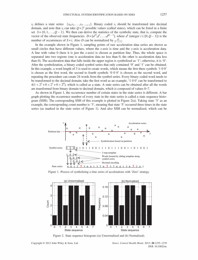
T�rþ1.In the example shown in Figure 1, sampling points of raw acceleration data series are shown as

small circles that have different values, where the x-axis is time and the y-axis is acceleration data.A line with value 0 (here it is just the x-axis) is chosen as partition line. Thus, the whole space isseparated into two regions (one is acceleration data no less than 0, the other is acceleration data lessthan 0). The acceleration data that falls inside the upper region is symbolized as ‘1’; otherwise, it is ‘0’.After the symbolization, a binary coded symbol series that only contained ‘0’ and ‘1’ can be obtained.In this example, a word length of 3 is used to create words, which means the first three symbols ‘1 0 0’is chosen as the first word, the second to fourth symbols ‘0 0 0’ is chosen as the second word, andrepeating the procedure can create 24 words from the symbol series. Every binary coded word needs tobe transformed to the decimal domain; take the first word as an example, ‘1 0 0’ can be transformed to4(1� 22 + 0� 21 + 0� 20), which is called as a state. A state series can be obtained after all the wordsare transformed from binary domain to decimal domain, which is composed of values 0~7.

As shown in Figure 1, the occurrence number of certain states in the state series is different. A bargraph plotting the occurrence number of every state in the state series is called a state sequence histo-gram (SSH). The corresponding SSH of this example is plotted in Figure 2(a). Taking state ‘5’ as anexample, the corresponding count number is ‘3’, meaning that state ‘5’ occurred three times in the stateseries (as marked in the state series of Figure 1). And also SSH can be normalized, which can be

5 54 0 1 2 3 6 4 1 3 7 6 3 7 6 4 1 3 6 5 2 4 1

Acceleration series

1 0 0 0 1 0 1 1 0 0 1 1 1 0 1 1 1 0 0 1 1 0 1 0 0 1

1 0 00 0 0

0 0 1

Partition line

Symbol series

State series

Symbolization based on partition

Decimal encoding

Words formed by sliding template along symbol series

3-step template

y

x

Figure 1. Process of symbolizing a time series of accelerations with ‘Zero’ strategy.

Figure 2. State sequence histogram ((a) Unnormalized and (b) Normalized).



accomplished by dividing the occurrence number of each state by the total number of states in thewhole state series, which is shown in Figure 2(b).

2.2. Types of symbolization strategy

There are different strategies for symbolizing a time series data; three of them will be introduced here.The difference among them is just the step of transforming the raw acceleration data to symbol series,but the other steps like choosing a word, transforming the binary coded word to decimal domain, andcalculating the SSH are unchanged; only the difference will be declared here.

The first one is called ‘Zero’ strategy, which can be explained by just using the example of Figure 1.The main specialty of this strategy is using a line with zero value as the partition line.

The second one is called ‘Mean’ strategy. The difference between the ‘Mean’ and the ‘Zero’ strategiesis that the ‘Mean’ strategy uses the line of mean value of the raw acceleration data series as partition lineinstead of a line with zero value in ‘Zero’ strategy.

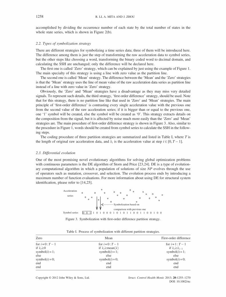
Obviously, the ‘Zero’ and ‘Mean’ strategies have a disadvantage as they may miss very detailedsignals. To represent such details, the third strategy, ‘first order difference’ strategy, should be used. Notethat for this strategy, there is no partition line like that used in ‘Zero’ and ‘Mean’ strategies. The mainprinciple of ‘first-order difference’ is contrasting every single acceleration value with the previous onefrom the second value of the raw acceleration series; if it is bigger than or equal to the previous one,one ‘1’ symbol will be created, else the symbol will be created as ‘0’. This strategy extracts details onthe composition from the signal, but it is affected by noise much more easily than the ‘Zero’ and ‘Mean’strategies are. The main procedure of first-order difference strategy is shown in Figure 3. Also, similar tothe procedure in Figure 1, words should be created from symbol series to calculate the SSH in the follow-ing steps.

The coding procedure of three partition strategies are summarized and listed in Table I, where T isthe length of original raw acceleration data, and €xi is the acceleration value at step i2 [0,T� 1].

2.3. Differential evolution

One of the most promising novel evolutionary algorithms for solving global optimization problemswith continuous parameters is the DE algorithm of Storn and Price [23,24]. DE is a type of evolution-ary computational algorithm in which a population of solutions of size NP evolves through the useof operators such as mutation, crossover, and selection. The evolution process ends by introducing amaximum number of function evaluations. For more information about using DE for structural systemidentification, please refer to [14,25].

0 0 1 1 0 1 0 0 0 1 0 1 0 1 1 0 0 1 1 0 0 1 0 0Symbol series

Symbolization based on

comparison with previous one

Acceleration

series

Figure 3. Symbolization with first-order difference partition strategy.

Table I. Process of symbolization with different partition strategies.

Zero Mean First-order difference

for i = 0 : T� 1 for i= 0 :T� 1 for i= 1 : T� 1if €xi≥0 if €xi≥mean €xð Þ if €xi≥€xi�1symbol(i) = 1; symbol(i) = 1; symbol(i) = 1;else else elsesymbol(i) = 0; symbol(i) = 0; symbol(i) = 0;end end endend end end



3. SYMBOLIZATION-BASED DIFFERENTIAL EVOLUTION STRATEGY

We devised a hybrid strategy, called the SDES, which combines the respective merits of STSA and DE.

3.1. Symbolization-based differential evolution strategy procedure

In the research field of structural system identification, usually a comparison of the time response of thesystem with that of a parameterized model using a norm or some performance criterion can give us ameasure of how well the model explains the system.

We will explain our SDES procedure using a physical system with input u and output y. Let y(ti)(i= 1, . . ., T) denote the value of the actual system at the ith discrete time step. Suppose that a param-eterized model able to capture the behavior of the physical system is developed and this model dependson a set of n parameters, that is, x ¼ x1; x2; . . . ; xnð ÞT 2 Rn. Given a candidate parameter value x and aguess X0 of the initial state, y tið Þ i ¼ 1; . . . ; Tð Þ, the value of the parameterized model, that is, the identifiedsystem at the ith discrete time step, can be obtained. Hence, the problem of system identification boilsdown to finding a set of parameters that minimize the prediction error between the system output y(ti),which is the measured data, and the model output y x; tið Þ; which is calculated at each time instant ti .

Usually our interest lies in minimizing the predefined error norm of the time series outputs, forexample, the following mean square error function,

f xð Þ ¼ 1T

XTi¼1

y tið Þ � y x; tið Þ2 (1)

where k � k represents the Euclidean norm of vectors. Formally, the optimization problem requires oneto find a set of n parameters x*2Rn, so that a certain quality criterion is satisfied, namely, that the errornorm f(•) is minimized. The function f(•) is called a fitness function or objective function. Typically, anobjective function that reflects the goodness of the solution is chosen. The identification problem canthus be treated as a linearly constrained multidimensional optimization problem, namely,

Minimize f xð Þ; x ¼ x1; x2; . . . ; xnð ÞT

s:t: x 2 S; S ¼ x : xmin;i⩽xi⩽xmax;i; 8i ¼ 1; 2; . . . ; n� �

(2)

where f(x) is an objective function that maps the decision variable x into the objective space f=Rn!R,S is an n-dimensional feasible search space, and xmax and xmin denote the upper and the lower bounds ofthe n parameters, respectively.

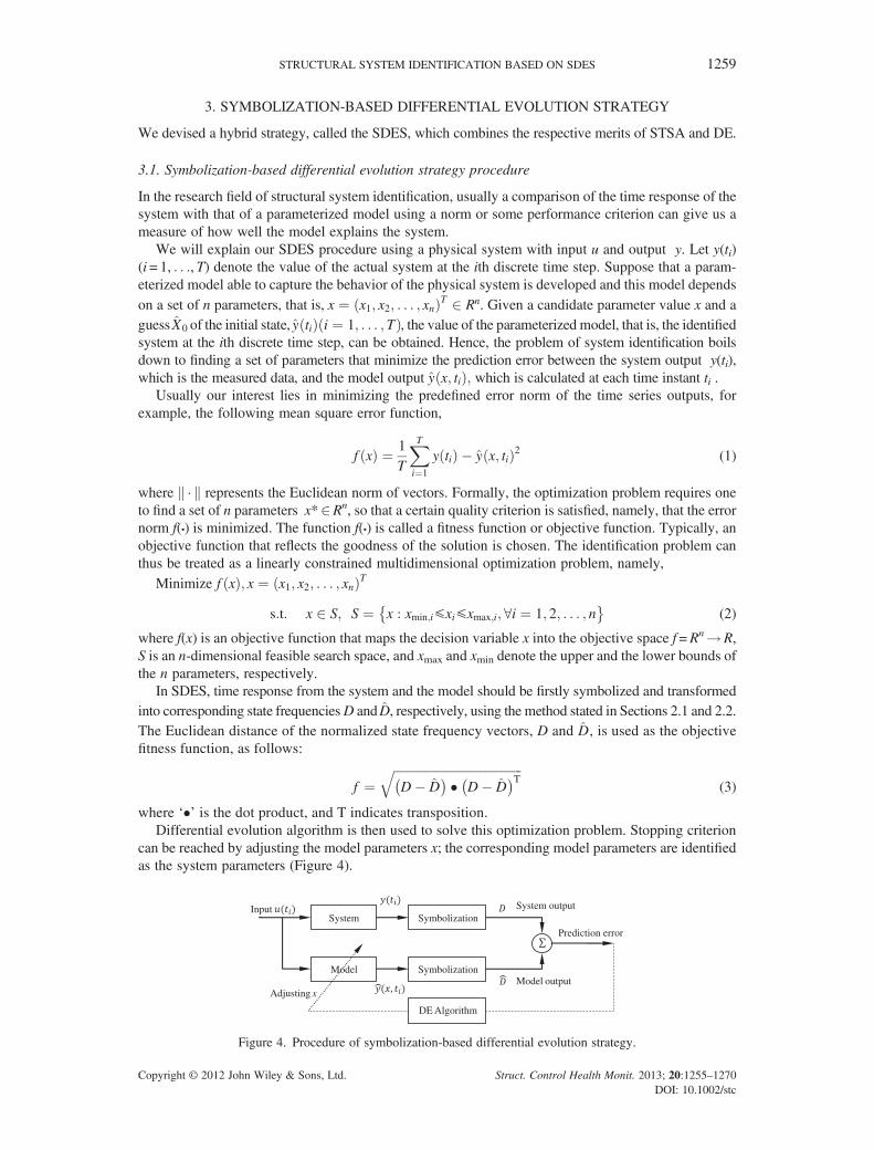
In SDES, time response from the system and the model should be firstly symbolized and transformedinto corresponding state frequenciesD and D, respectively, using the method stated in Sections 2.1 and 2.2.The Euclidean distance of the normalized state frequency vectors, D and D, is used as the objectivefitness function, as follows:

f ¼ffiffiffiffiffiffiffiffiffiffiffiffiffiffiffiffiffiffiffiffiffiffiffiffiffiffiffiffiffiffiffiffiffiffiffiffiffiffiffiffiffiffiD� D� � � D� D

� �Tq(3)

where ‘�’ is the dot product, and T indicates transposition.Differential evolution algorithm is then used to solve this optimization problem. Stopping criterion

can be reached by adjusting the model parameters x; the corresponding model parameters are identifiedas the system parameters (Figure 4).

System

Model

Symbolization

Symbolization

DE Algorithm

System output

Model output

Prediction error

Input

Adjusting x

Figure 4. Procedure of symbolization-based differential evolution strategy.



3.2. Solution range

As a coarse-graining process, the symbolization procedure can extract representative dynamic featuresof a structural system, but in so doing it may lose the details. However, with suitable partitioning andappropriate choice of STSA parameters, it has been observed that information necessary for accurateestimation is retained in symbol sequences [26].

Transforming raw acceleration data into SSH probably leads to a new relationship between the index(SSH) and structure parameters, which is many-to-one correspondence. If all of the candidate solutions ina solution space create the same SSH, all candidate solutions in this area are indistinguishable.We call thisarea ‘solution range’. The deviation between candidate solutions in ‘solution range’ and true solutionbrings the problemwhether the solution can be reliable or not. Obviously, if the solution range is too wide,the accuracy of the proposed procedure will be affected. If the solution range is small enough, the candi-date solutions in ‘solution range’ are close to the true solution. Thus, the accuracy may be satisfactory.

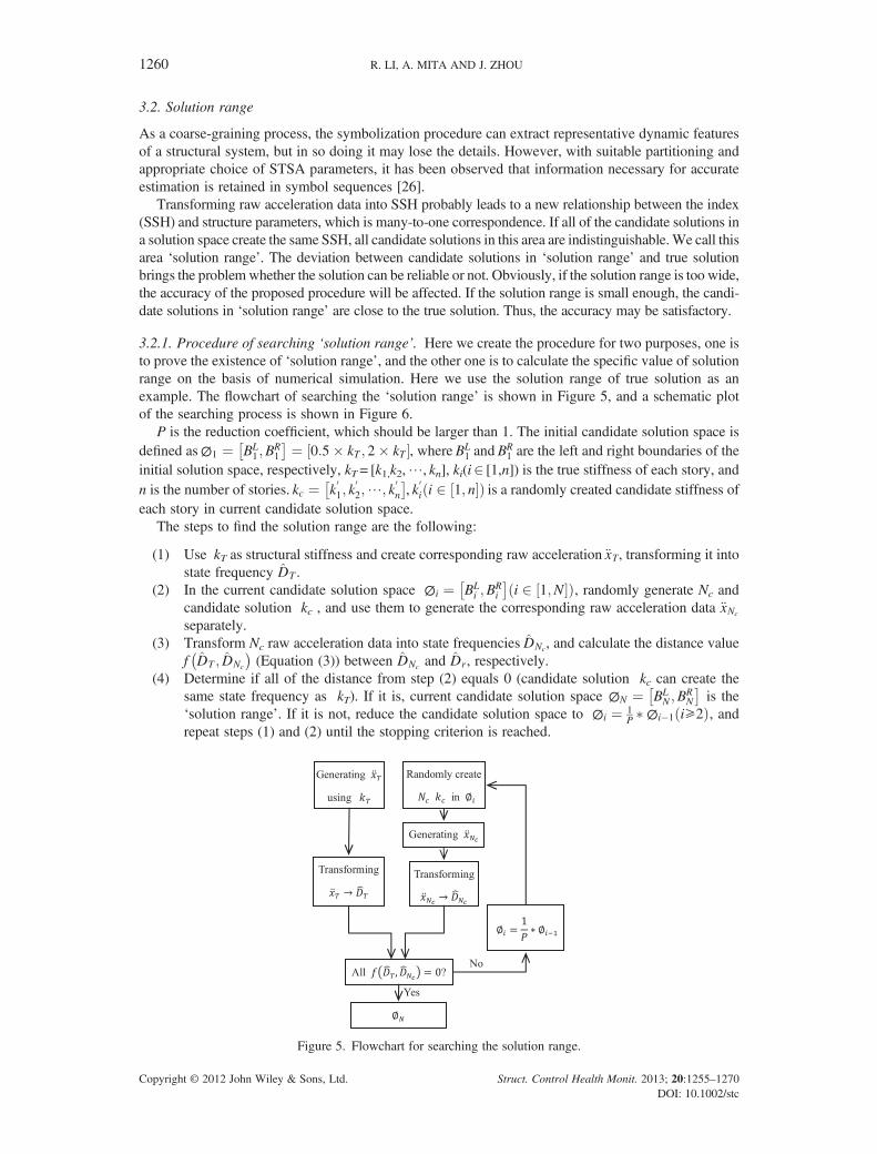
3.2.1. Procedure of searching ‘solution range’. Here we create the procedure for two purposes, one isto prove the existence of ‘solution range’, and the other one is to calculate the specific value of solutionrange on the basis of numerical simulation. Here we use the solution range of true solution as anexample. The flowchart of searching the ‘solution range’ is shown in Figure 5, and a schematic plotof the searching process is shown in Figure 6.

P is the reduction coefficient, which should be larger than 1. The initial candidate solution space isdefined as∅1 ¼ BL

1 ;BR1

� � ¼ 0:5� kT ; 2� kT½ �, where BL1 and B

R1 are the left and right boundaries of the

initial solution space, respectively, kT= [k1,k2,⋯, kn], ki(i2 [1,n]) is the true stiffness of each story, andn is the number of stories. kc ¼ k

01; k

02;⋯; k

0n

� �, k

0i i 2 1; n½ �ð Þ is a randomly created candidate stiffness of

each story in current candidate solution space.The steps to find the solution range are the following:

(1) Use kT as structural stiffness and create corresponding raw acceleration €xT, transforming it intostate frequency DT .

(2) In the current candidate solution space ∅i ¼ BLi ;B

Ri

� �i 2 1;N½ �ð Þ, randomly generate Nc and

candidate solution kc , and use them to generate the corresponding raw acceleration data €xNc

separately.(3) Transform Nc raw acceleration data into state frequencies DNc, and calculate the distance value

f DT ; DNc

� �(Equation (3)) between DNc and Dr , respectively.

(4) Determine if all of the distance from step (2) equals 0 (candidate solution kc can create thesame state frequency as kT). If it is, current candidate solution space ∅N ¼ BL

N ;BRN

� �is the

‘solution range’. If it is not, reduce the candidate solution space to ∅i ¼ 1P �∅i�1 i⩾2ð Þ, and

repeat steps (1) and (2) until the stopping criterion is reached.

Figure 5. Flowchart for searching the solution range.


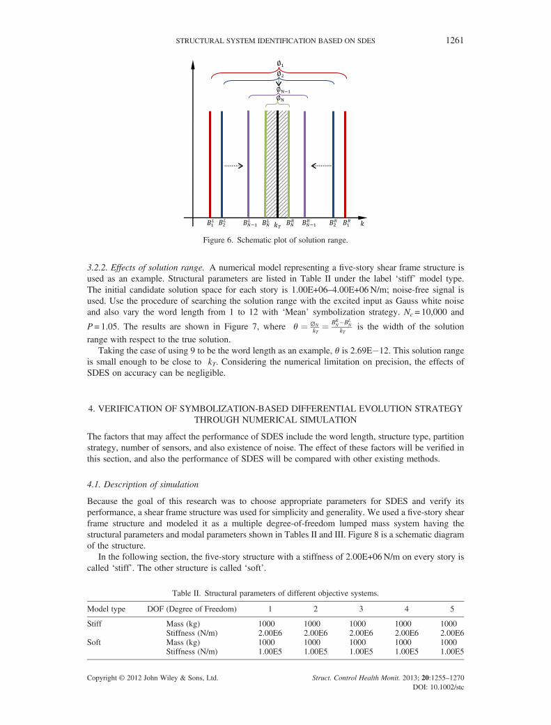
Figure 6. Schematic plot of solution range.


3.2.2. Effects of solution range. A numerical model representing a five-story shear frame structure isused as an example. Structural parameters are listed in Table II under the label ‘stiff’ model type.The initial candidate solution space for each story is 1.00E+06–4.00E+06N/m; noise-free signal isused. Use the procedure of searching the solution range with the excited input as Gauss white noiseand also vary the word length from 1 to 12 with ‘Mean’ symbolization strategy. Nc = 10,000 and

P= 1.05. The results are shown in Figure 7, where θ ¼ ∅NkT¼ BR

N�BLN

kTis the width of the solution

range with respect to the true solution.Taking the case of using 9 to be the word length as an example, θ is 2.69E�12. This solution range

is small enough to be close to kT. Considering the numerical limitation on precision, the effects ofSDES on accuracy can be negligible.

4. VERIFICATION OF SYMBOLIZATION-BASED DIFFERENTIAL EVOLUTION STRATEGYTHROUGH NUMERICAL SIMULATION

The factors that may affect the performance of SDES include the word length, structure type, partitionstrategy, number of sensors, and also existence of noise. The effect of these factors will be verified inthis section, and also the performance of SDES will be compared with other existing methods.

4.1. Description of simulation

Because the goal of this research was to choose appropriate parameters for SDES and verify itsperformance, a shear frame structure was used for simplicity and generality. We used a five-story shearframe structure and modeled it as a multiple degree-of-freedom lumped mass system having thestructural parameters and modal parameters shown in Tables II and III. Figure 8 is a schematic diagramof the structure.

In the following section, the five-story structure with a stiffness of 2.00E+06N/m on every story iscalled ‘stiff’. The other structure is called ‘soft’.

Table II. Structural parameters of different objective systems.

Model type DOF (Degree of Freedom) 1 2 3 4 5

Stiff Mass (kg) 1000 1000 1000 1000 1000Stiffness (N/m) 2.00E6 2.00E6 2.00E6 2.00E6 2.00E6

Soft Mass (kg) 1000 1000 1000 1000 1000Stiffness (N/m) 1.00E5 1.00E5 1.00E5 1.00E5 1.00E5


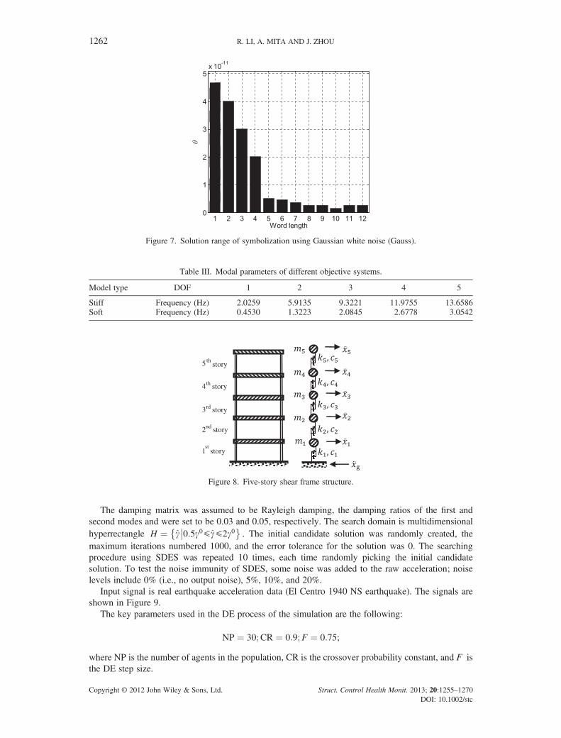
Figure 7. Solution range of symbolization using Gaussian white noise (Gauss).

Table III. Modal parameters of different objective systems.

Model type DOF 1 2 3 4 5

Stiff Frequency (Hz) 2.0259 5.9135 9.3221 11.9755 13.6586Soft Frequency (Hz) 0.4530 1.3223 2.0845 2.6778 3.0542

3rd story

2nd story

1st

story

4th story

5thstory

Figure 8. Five-story shear frame structure.


The damping matrix was assumed to be Rayleigh damping, the damping ratios of the first andsecond modes and were set to be 0.03 and 0.05, respectively. The search domain is multidimensionalhyperrectangle H ¼ g 0:5g0⩽g⩽2g0

��. The initial candidate solution was randomly created, the

maximum iterations numbered 1000, and the error tolerance for the solution was 0. The searchingprocedure using SDES was repeated 10 times, each time randomly picking the initial candidatesolution. To test the noise immunity of SDES, some noise was added to the raw acceleration; noiselevels include 0% (i.e., no output noise), 5%, 10%, and 20%.

Input signal is real earthquake acceleration data (El Centro 1940 NS earthquake). The signals areshown in Figure 9.

The key parameters used in the DE process of the simulation are the following:

NP ¼ 30;CR ¼ 0:9;F ¼ 0:75;

where NP is the number of agents in the population, CR is the crossover probability constant, and F isthe DE step size.


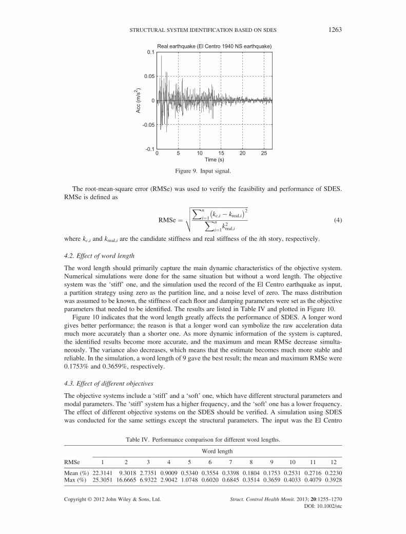
Figure 9. Input signal.


The root-mean-square error (RMSe) was used to verify the feasibility and performance of SDES.RMSe is defined as

RMSe ¼ffiffiffiffiffiffiffiffiffiffiffiffiffiffiffiffiffiffiffiffiffiffiffiffiffiffiffiffiffiffiffiffiffiffiffiffiffiffiffiffiXn

i¼1kc;i � kreal;i� �2

Xn

i¼1k2real;i

vuut (4)

where kc,i and kreal,i are the candidate stiffness and real stiffness of the ith story, respectively.

4.2. Effect of word length

The word length should primarily capture the main dynamic characteristics of the objective system.Numerical simulations were done for the same situation but without a word length. The objectivesystem was the ‘stiff’ one, and the simulation used the record of the El Centro earthquake as input,a partition strategy using zero as the partition line, and a noise level of zero. The mass distributionwas assumed to be known, the stiffness of each floor and damping parameters were set as the objectiveparameters that needed to be identified. The results are listed in Table IV and plotted in Figure 10.

Figure 10 indicates that the word length greatly affects the performance of SDES. A longer wordgives better performance; the reason is that a longer word can symbolize the raw acceleration datamuch more accurately than a shorter one. As more dynamic information of the system is captured,the identified results become more accurate, and the maximum and mean RMSe decrease simulta-neously. The variance also decreases, which means that the estimate becomes much more stable andreliable. In the simulation, a word length of 9 gave the best result; the mean and maximum RMSe were0.1753% and 0.3659%, respectively.

4.3. Effect of different objectives

The objective systems include a ‘stiff’ and a ‘soft’ one, which have different structural parameters andmodal parameters. The ‘stiff’ system has a higher frequency, and the ‘soft’ one has a lower frequency.The effect of different objective systems on the SDES should be verified. A simulation using SDESwas conducted for the same settings except the structural parameters. The input was the El Centro

Table IV. Performance comparison for different word lengths.

RMSe

Word length

1 2 3 4 5 6 7 8 9 10 11 12

Mean (%) 22.3141 9.3018 2.7351 0.9009 0.5340 0.3554 0.3398 0.1804 0.1753 0.2531 0.2716 0.2230Max (%) 25.3051 16.6665 6.9322 2.9042 1.0748 0.6020 0.6845 0.3514 0.3659 0.4033 0.4079 0.3928


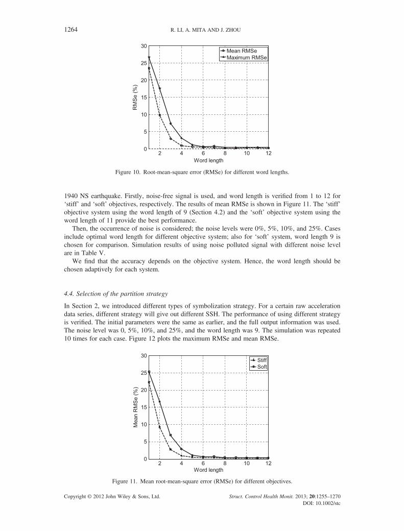
Figure 10. Root-mean-square error (RMSe) for different word lengths.


1940 NS earthquake. Firstly, noise-free signal is used, and word length is verified from 1 to 12 for‘stiff’ and ‘soft’ objectives, respectively. The results of mean RMSe is shown in Figure 11. The ‘stiff’objective system using the word length of 9 (Section 4.2) and the ‘soft’ objective system using theword length of 11 provide the best performance.

Then, the occurrence of noise is considered; the noise levels were 0%, 5%, 10%, and 25%. Casesinclude optimal word length for different objective system; also for ‘soft’ system, word length 9 ischosen for comparison. Simulation results of using noise polluted signal with different noise levelare in Table V.

We find that the accuracy depends on the objective system. Hence, the word length should bechosen adaptively for each system.

4.4. Selection of the partition strategy

In Section 2, we introduced different types of symbolization strategy. For a certain raw accelerationdata series, different strategy will give out different SSH. The performance of using different strategyis verified. The initial parameters were the same as earlier, and the full output information was used.The noise level was 0, 5%, 10%, and 25%, and the word length was 9. The simulation was repeated10 times for each case. Figure 12 plots the maximum RMSe and mean RMSe.

Figure 11. Mean root-mean-square error (RMSe) for different objectives.


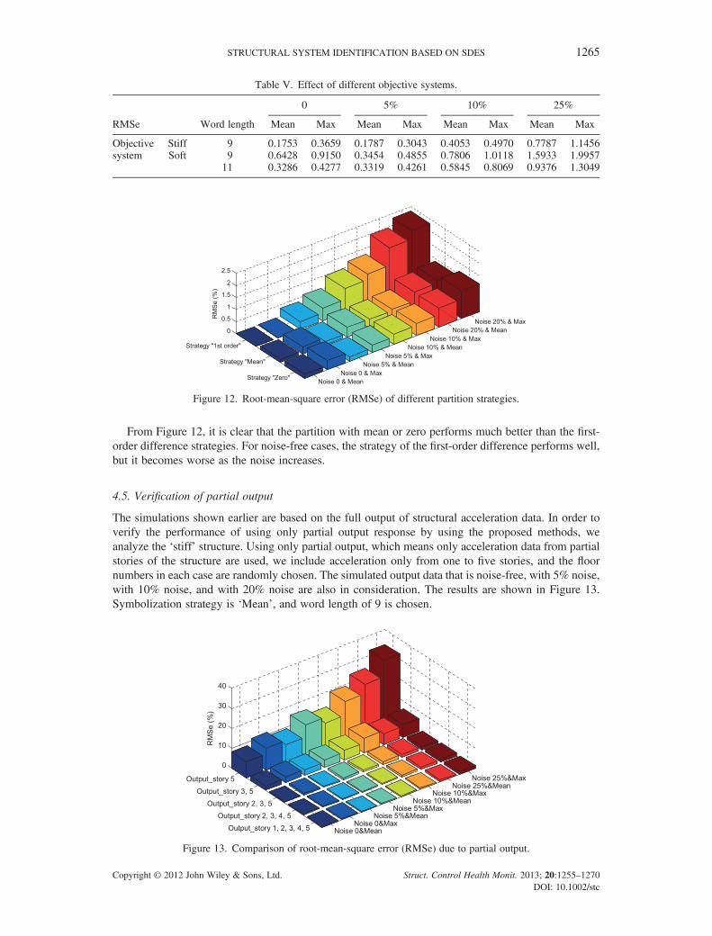
Table V. Effect of different objective systems.

0 5% 10% 25%

RMSe Word length Mean Max Mean Max Mean Max Mean Max

Objectivesystem

Stiff 9 0.1753 0.3659 0.1787 0.3043 0.4053 0.4970 0.7787 1.1456Soft 9 0.6428 0.9150 0.3454 0.4855 0.7806 1.0118 1.5933 1.9957

11 0.3286 0.4277 0.3319 0.4261 0.5845 0.8069 0.9376 1.3049

Figure 12. Root-mean-square error (RMSe) of different partition strategies.


From Figure 12, it is clear that the partition with mean or zero performs much better than the first-order difference strategies. For noise-free cases, the strategy of the first-order difference performs well,but it becomes worse as the noise increases.

4.5. Verification of partial output

The simulations shown earlier are based on the full output of structural acceleration data. In order toverify the performance of using only partial output response by using the proposed methods, weanalyze the ‘stiff’ structure. Using only partial output, which means only acceleration data from partialstories of the structure are used, we include acceleration only from one to five stories, and the floornumbers in each case are randomly chosen. The simulated output data that is noise-free, with 5% noise,with 10% noise, and with 20% noise are also in consideration. The results are shown in Figure 13.Symbolization strategy is ‘Mean’, and word length of 9 is chosen.

Figure 13. Comparison of root-mean-square error (RMSe) due to partial output.


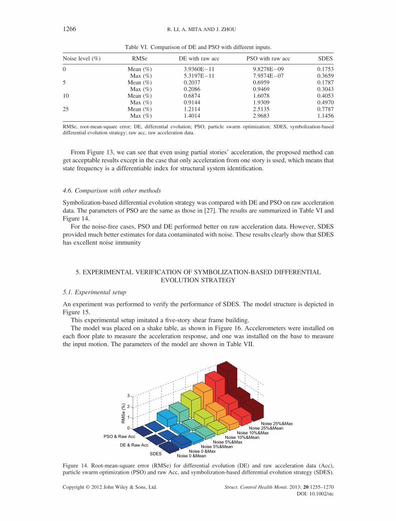
Table VI. Comparison of DE and PSO with different inputs.

Noise level (%) RMSe DE with raw acc PSO with raw acc SDES

0 Mean (%) 3.9360E�11 9.8278E�09 0.1753Max (%) 5.3197E�11 7.9574E�07 0.3659

5 Mean (%) 0.2037 0.6959 0.1787Max (%) 0.2086 0.9469 0.3043

10 Mean (%) 0.6874 1.6078 0.4053Max (%) 0.9144 1.9309 0.4970

25 Mean (%) 1.2114 2.5135 0.7787Max (%) 1.4014 2.9683 1.1456

RMSe, root-mean-square error; DE, differential evolution; PSO, particle swarm optimization; SDES, symbolization-baseddifferential evolution strategy; raw acc, raw acceleration data.


From Figure 13, we can see that even using partial stories’ acceleration, the proposed method canget acceptable results except in the case that only acceleration from one story is used, which means thatstate frequency is a differentiable index for structural system identification.

4.6. Comparison with other methods

Symbolization-based differential evolution strategy was compared with DE and PSO on raw accelerationdata. The parameters of PSO are the same as those in [27]. The results are summarized in Table VI andFigure 14.

For the noise-free cases, PSO and DE performed better on raw acceleration data. However, SDESprovided much better estimates for data contaminated with noise. These results clearly show that SDEShas excellent noise immunity

5. EXPERIMENTAL VERIFICATION OF SYMBOLIZATION-BASED DIFFERENTIALEVOLUTION STRATEGY

5.1. Experimental setup

An experiment was performed to verify the performance of SDES. The model structure is depicted inFigure 15.

This experimental setup imitated a five-story shear frame building.The model was placed on a shake table, as shown in Figure 16. Accelerometers were installed on

each floor plate to measure the acceleration response, and one was installed on the base to measurethe input motion. The parameters of the model are shown in Table VII.

Figure 14. Root-mean-square error (RMSe) for differential evolution (DE) and raw acceleration data (Acc),particle swarm optimization (PSO) and raw Acc, and symbolization-based differential evolution strategy (SDES).


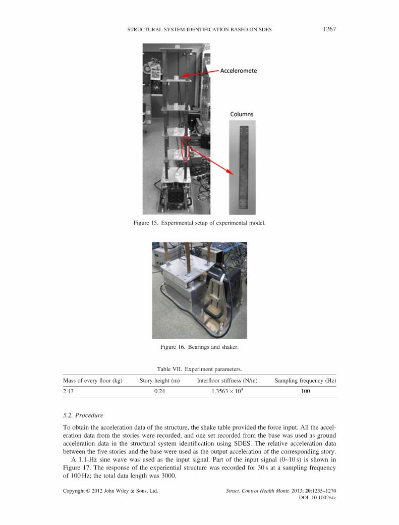
Figure 15. Experimental setup of experimental model.

Figure 16. Bearings and shaker.

Table VII. Experiment parameters.

Mass of every floor (kg) Story height (m) Interfloor stiffness (N/m) Sampling frequency (Hz)

2.43 0.24 1.3563� 104 100


5.2. Procedure

To obtain the acceleration data of the structure, the shake table provided the force input. All the accel-eration data from the stories were recorded, and one set recorded from the base was used as groundacceleration data in the structural system identification using SDES. The relative acceleration databetween the five stories and the base were used as the output acceleration of the corresponding story.

A 1.1-Hz sine wave was used as the input signal. Part of the input signal (0~10 s) is shown inFigure 17. The response of the experiential structure was recorded for 30 s at a sampling frequencyof 100Hz; the total data length was 3000.


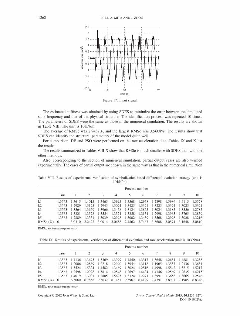
Figure 17. Input signal.


The estimated stiffness was obtained by using SDES to minimize the error between the simulatedstate frequency and that of the physical structure. The identification process was repeated 10 times.The parameters of SDES were the same as those in the numerical simulation. The results are shownin Table VIII; The unit is 10 kN/m.

The average of RMSe was 2.9437%, and the largest RMSe was 3.5608%. The results show thatSDES can identify the structural parameters of the model quite well.

For comparison, DE and PSO were performed on the raw acceleration data. Tables IX and X listthe results.

The results summarized in Tables VIII-X show that RMSe is much smaller with SDES than with theother methods.

Also, corresponding to the section of numerical simulation, partial output cases are also verifiedexperimentally. The cases of partial output are chosen in the same way as that in the numerical simulation

Table VIII. Results of experimental verification of symbolization-based differential evolution strategy (unit is10 kN/m).

Process number

True 1 2 3 4 5 6 7 8 9 10

k1 1.3563 1.3615 1.4015 1.3465 1.3995 1.3568 1.2958 1.2898 1.3986 1.4115 1.3528k2 1.3563 1.2989 1.3125 1.2945 1.3024 1.3425 1.3321 1.3225 1.3324 1.3025 1.3321k3 1.3563 1.3564 1.3669 1.3966 1.3458 1.3124 1.3865 1.3024 1.3185 1.3556 1.2785k4 1.3563 1.3321 1.3528 1.3554 1.3324 1.3358 1.3154 1.2998 1.3965 1.3765 1.3859k5 1.3563 1.2889 1.3331 1.3039 1.2998 1.3002 1.3459 1.3568 1.2998 1.3028 1.3216RMSe (%) 0 3.0310 2.2422 3.0014 3.0658 2.4862 2.7467 3.5608 3.0574 3.1648 3.0810

RMSe, root-mean-square error.

Table IX. Results of experimental verification of differential evolution and raw acceleration (unit is 10 kN/m).

Process number

True 1 2 3 4 5 6 7 8 9 10

k1 1.3563 1.4136 1.3695 1.3369 1.3999 1.4850 1.3317 1.3658 1.2654 1.4881 1.3258k2 1.3563 1.2006 1.2869 1.2218 1.2990 1.5954 1.3118 1.1965 1.3557 1.2136 1.3654k3 1.3563 1.3524 1.5324 1.4582 1.3469 1.3024 1.2516 1.4998 1.5542 1.3215 1.5217k4 1.3563 1.2598 1.2998 1.5814 1.2548 1.2697 1.4434 1.4146 1.2569 1.2635 1.4215k5 1.3563 1.4019 1.3001 1.2885 1.5695 1.3324 1.2271 1.3991 1.3658 1.3665 1.2546RMSe (%) 0 6.5060 6.7858 9.5632 8.1457 9.5967 6.4129 7.4791 7.8997 7.1985 6.8346



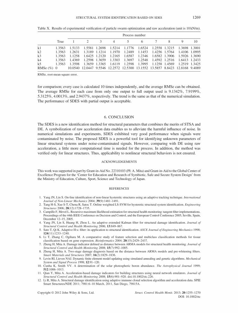
Table X. Results of experimental verification of particle swarm optimization and raw acceleration (unit is 10 kN/m).

Process number

True 1 2 3 4 5 6 7 8 9 10

k1 1.3563 1.5133 1.5581 1.2698 1.5214 1.1776 1.6524 1.2558 1.3215 1.3698 1.3001k2 1.3563 1.2631 1.3189 1.1214 1.1970 1.2489 1.1453 1.4256 1.5764 1.4106 1.0995k3 1.3563 1.1258 1.6425 1.2120 1.2165 1.6587 1.2346 1.6582 1.3906 1.5926 1.3690k4 1.3563 1.4369 1.2598 1.3659 1.3303 1.3697 1.2548 1.4592 1.2516 1.6413 1.2433k5 1.3563 1.3598 1.3659 1.3365 1.6119 1.2598 1.3995 1.1258 1.4569 1.2519 1.3425RMSe (%) 0 10.0540 12.0447 9.5546 12.2572 12.5300 13.1552 13.5857 8.8423 12.8168 9.4089



for comparison; every case is calculated 10 times independently, and the average RMSe can be obtained.The average RMSe for each case from only one output to full output used is 9.1342%, 7.9199%,5.3125%, 4.0013%, and 2.9437%, respectively. The trend is the same as that of the numerical simulation.The performance of SDES with partial output is acceptable.

6. CONCLUSION

The SDES is a new identification method for structural parameters that combines the merits of STSA andDE. A symbolization of raw acceleration data enables us to alleviate the harmful influence of noise. Innumerical simulations and experiments, SDES exhibited very good performance when signals werecontaminated by noise. The proposed SDES is a powerful tool for identifying unknown parameters oflinear structural systems under noise-contaminated signals. However, comparing with DE using rawacceleration, a little more computational time is needed for the process. In addition, the method wasverified only for linear structures. Thus, applicability to nonlinear structural behaviors is not ensured.

ACKNOWLEDGEMENTS

This work was supported in part by Grant-in-AidNo. 22310103 (PI: A.Mita) and Grant-in-Aid to the Global Center ofExcellence Program for the ‘Center for Education and Research of Symbiotic, Safe and Secure System Design’ fromthe Ministry of Education, Culture, Sport, Science and Technology of Japan.

REFERENCES

1. Yang JN, Lin S. On-line identification of non-linear hysteretic structures using an adaptive tracking technique. InternationalJournal of Non-Linear Mechanics 2004; 39(9):1481–1491.

2. Tang H-S, Xue S-T, Chena R, Satoc T. Online weighted LS-SVM for hysteretic structural system identification. EngineeringStructures 2006; 28(12):1728–1735.

3. Campillo F,Mevel L. Recursive maximum likelihood estimation for structural health monitoring: tangent filter implementations.Proceedings of the 44th IEEE Conference on Decision and Control, and the European Control Conference 2005; Seville, Spain,December 12–15, 2005.

4. Yang JN, Lin S, Huang H, Zhou L. An adaptive extended Kalman filter for structural damage identification. Journal ofStructural Control and Health Monitoring 2006; 13:849–867.

5. Sato T, Qi K. Adaptive H1 filter: its application to structural identification. ASCE Journal of Engineering Mechanics 1998;124(11):1233–1240.

6. Li T, Zhang C, Ogihara M. A comparative study of feature selection and multiclass classification methods for tissueclassification based on gene expression. Bioinformatics 2004; 20(15):2429–2437.

7. Zheng H, Mita A. Damage indicator defined as distance between ARMA models for structural health monitoring. Journal ofStructural Control and Health Monitoring 2008; 15(7):992–1005.

8. Zheng H, Mita A. Two-stage damage diagnosis based on the distance between ARMA models and pre-whitening filters.Smart Materials and Structures 2007; 16(2):1829–1836.

9. Levin RI, Lieven NAJ. Dynamic finite element model updating using simulated annealing and genetic algorithms. MechanicalSystem and Signal Process 1998; 12:91–120.

10. Cunha K, Smith VV. A determination of the solar photospheric boron abundance. The Astrophysical Journal 1999;512:1006–1013.

11. Qian Y, Mita A. Acceleration-based damage indicators for building structures using neural network emulators. Journal ofStructural Control and Health Monitoring 2008; 15(6):901–920. doi:10.1002/stc.226.

12. Li R, Mita A. Structural damage identification using adaptive immune clonal selection algorithm and acceleration data. SPIESmart Structures/NDE 2011; 7981:6–10 March, 2011, San Diego, 79815A.



13. Ursem RK, Vadstrup P. Parameter identification of induction motors using differential evolution. Proceedings of the FifthCongress on Evolutionary Computation (CEC-2003); 790–796.

14. Tang H, Xue S, Fan C. Differential evolution strategy for structural system identification. Computers and Structures 2008;86:2004–2012.

15. Wan C, Mita A. Pipeline monitoring using acoustic principal component analysis recognition with the Mel scale. SmartMaterials and Structures 2009; 18:1–11.

16. Ray. Symbolic dynamic analysis of complex systems for anomaly detection. Signal Processing 2004; 84(7):1115–1130.17. Chin S, Ray A, Rajagopalan V. Symbolic time series analysis for anomaly detection: a comparative evaluation. Signal

Processing 2005; 85(9):1859–1868.18. Khatkhate A, Ray A, Chin S, Rajagopalan V, Keller E. Detection of fatigue crack anomaly: a symbolic dynamic approach,

Proceedings of American Control Conference, Boston, MA, June–July 2004; 3741–3746.19. Tolani D, Yasar M, Ray A, Yang V. Anomaly detection in aircraft gas turbine engines. AIAA Journal of Aerospace

Computing Information, and Communication 2006; 3:44–51.20. Bhatnagar S, Rajagopalan V, Ray A. Incipient fault detection in mechanical power transmission systems. Proceedings of

American Control Conference, Portland, OR, June 2005; 472–477.21. Samsi R, Rajagopalan V, Mayer J, Ray A. Early detection of voltage imbalances in induction machines, Proceedings of

American Control Conference, Portland, OR, June 2005; 478–483.22. Rajagopalan V, Ray A. Symbolic time series analysis via wavelet-based partitioning. Signal Processing November 2006;

86(11):3309–3320.23. Storn R, Price K. Differential evolution-a simple and efficient adaptive scheme for global optimization over continuous

spaces. Technical Rep. No. TR-95-012, International Computer Science Institute, Berkley (CA); 1995.24. Storn R, Price K. Minimizing the real functions of the ICEC’96 contest by differential evolution. In Proceedings of the IEEE

international conference on evolutionary computation, Nagoya, Japan; 1996.25. Liao TW. Two hybrid differential evolution algorithms for engineering design optimization. Applied Soft Computing 2010;

10:1188–1199.26. Rajagopalan V, Chakraborty S, Ray A. Estimation of slowly varying parameters in nonlinear systems via symbolic dynamic

filtering. Signal Processing February 2008; 88(2):339–348.27. Xue S, Tang H, Zhou J. Identification of structural systems using particle swarm optimization. Journal of Asian Architecture

and Building Engineering November 2009; 8(2):517–524.


symbolization-based differential evolution strategy for identification of structural parameters

Documents