symbolic time series analysis of ultrasonic data for early

ARTICLE IN PRESS

Mechanical Systemsand

Signal Processing

0888-3270/$ - se

doi:10.1016/j.ym

$This work�CorrespondE-mail addr

Mechanical Systems and Signal Processing 21 (2007) 866–884

www.elsevier.com/locate/jnlabr/ymssp

Symbolic time series analysis of ultrasonic data for earlydetection of fatigue damage$

Shalabh Gupta�, Asok Ray, Eric Keller

The Pennsylvania State University, University Park, PA 16802, USA

Received 8 July 2005; received in revised form 20 August 2005; accepted 22 August 2005

Available online 19 October 2005

Abstract

This paper presents a novel analytical tool for early detection of fatigue damage in polycrystalline alloys that are

commonly used in mechanical structures. Time series data of ultrasonic sensors have been used for anomaly detection in

the statistical behaviour of structural materials, where the analysis is based on the principles of symbolic dynamics and

automata theory. The performance of the proposed method has been evaluated relative to existing pattern recognition tools,

such as neural networks and principal component analysis, for detection of small changes in the statistical characteristics of

the observed data sequences. This concept is experimentally validated on a special-purpose test apparatus for 7075-T6

aluminium alloy specimens, where the anomalies accrue from small fatigue crack growth.

r 2005 Elsevier Ltd. All rights reserved.

Keywords: Symbolic time series analysis; Pattern recognition; Neural networks; Anomaly detection

1. Introduction

Gradually evolving changes in the structural parameters of a mechanical system over its service life maygenerate uncertainties in both dynamic and stationary behaviour. This problem is often addressed by overlyconservative estimates of the critical design parameters due to lack of available information. Consequently,the engineering design of mechanical systems suffers from enforcement of large safety factors and results inmanufacture of cumbersome and unnecessarily expensive machinery.

Material irregularities, uncertain usage patterns (e.g. random overloads and sudden jerks) andenvironmental conditions (e.g. fluctuations in temperature and humidity) may adversely affect the servicelife of mechanical systems to cause performance degradation and unanticipated failures. Damage due tofatigue crack is one of the most commonly encountered sources of structural degradation during both nominaland off-nominal operations in mechanical systems [1]. If not detected at an early stage, the accumulatedfatigue damage could potentially cause catastrophic failures in the system, leading to loss of human life andexpensive equipment. Therefore, for reliable operation and enhanced availability, it is necessary to develop

e front matter r 2005 Elsevier Ltd. All rights reserved.

ssp.2005.08.022

has been supported in part by Army Research Office (ARO) under Grant No. DAAD19-01-1-0646.

ing author.

esses: [email protected] (S. Gupta), [email protected] (A. Ray), [email protected] (E. Keller).

www.elsevier.com/locate/jnlabr/ymssp

ARTICLE IN PRESSS. Gupta et al. / Mechanical Systems and Signal Processing 21 (2007) 866–884 867

capabilities for prognosis of impending failures, such as the onset of wide-spread crack damage in criticalstructures. In the current state-of-the-art, direct measurements of fatigue damage at an early stage (e.g. crackinitiation) are not feasible due to lack of appropriate sensing devices and analytical models. This paperattempts to address this inadequacy by taking advantage of advanced signal processing and patternrecognition tools. Since a vast majority of structural components that are prone to fatigue damage are made ofpolycrystalline alloys [1], the paper focuses on fatigue damage sensing and prediction for such materials.

Sole reliance on model-based analysis for structural damage monitoring is infeasible because of thedifficulty in achieving requisite accuracy in modelling of fatigue damage evolution. For example, no existingmodel can capture the dynamical behaviour of fatigue damage at the grain level based on the basicfundamentals of molecular physics. In general, these models are critically dependent on the initial defects inthe materials, which may randomly form crack nucleation sites. Small deviations in the distribution of initialdefects may produce large variations in the evolution of fatigue damage for (apparently) identical specimensunder the same loading and environmental conditions [2]. The stochastic nature of fatigue damage stresses theneed for online updating of information using various sensing devices which can provide useful estimate offatigue damage and are capable of issuing early warnings. Consequently, the analysis of time series data [3]from the available sensors mounted on the critical machinery components, is essential for tracking thebehaviour pattern of the evolving fatigue damage in real time. Recent literature has demonstrated fatiguecrack monitoring using sensor-based information [4,5]. Ultrasonic sensing techniques were applied for fatiguecrack detection but they lacked precise signal processing capabilities for small change detection. Informationfrom multiple (e.g. ultrasonic and acoustic emission) sensors was used for fatigue crack monitoring [6] and theresults were shown to be in good agreement. However, the issues of early detection and real-time continuoushealth monitoring were not addressed.

Various signal processing applications deal with the analysis of time series data and attempts have beenmade to extract maximum useful information from the ensemble of sensor data. The problem of featureextraction from time series data for structural health monitoring has been recently addressed by manyresearchers [7–9]. The tools of statistical pattern recognition, auto-regressive model analysis, and waveletanalysis were applied to classify faults by different data patterns. However, the critical issue of detectinggradually evolving faults in real time were not addressed. Moreover, no quantifying measure was provided fordamage accumulation and growth rate based on statistical information. Recently, techniques of non-lineardynamics have been applied for structural health monitoring [10–12] based on the concepts of attractor-basedcross-prediction error between the measured signal and its predicted value. However, since dimension of thephase space may grow unbounded for noisy data, the analysis could be computationally expensive andinfeasible for real-time applications. Furthermore, dealing with high dimensions might lead to spurious resultsand dimension reduction may lead to loss of vital information. To alleviate these difficulties, this paper hasadopted a novel method of wavelet-based partitioning [13,14]. Based on this partitioning, the pertinentinformation is extracted from time series data sets in the form of probability distributions. Slight deviations inthese distributions from that under the nominal condition is captured to identify the damage pattern.

Anomaly detection using symbolic time series analysis (STSA) [15] is a pattern recognition method that hasbeen recently developed based upon a fixed-structure, fixed-order Markov chain, called the D-Markov machine

[13]. This paper presents and experimentally validates this novel concept of fatigue damage prediction for earlydetection of anomalous patterns in the sensor data. The proposed STSA-based technique is evaluated relativeto existing pattern recognition tools, such as neural networks and principal component analysis, for detection ofstatistical behaviour changes in the observed data sequence. The experimental platform is a fatigue testingapparatus, where possible anomalies accrue from the growth of small fatigue damage in 7075-T6 aluminiumalloy specimens.

The paper is organised in seven sections. Section 2 formulates the problem of anomaly detection andsummarises the concept of anomaly detection via symbolic time series analysis [13]. Section 3 describes thedetails of the experimental apparatus and outlines the basic features of optical microscopy and ultrasonicsensing. Brief descriptions of existing pattern recognition techniques are given in Section 4 and the algorithmof D-Markov machine construction is presented in Section 5. The details of data collection and analysis, asneeded for experimental validation of the proposed concept, is described in Section 6. The results, derivedfrom the test data, are presented to make a comparative evaluation of the proposed method with other pattern

ARTICLE IN PRESSS. Gupta et al. / Mechanical Systems and Signal Processing 21 (2007) 866–884868

recognition techniques from the perspectives of early detection of fatigue damage. Section 7 summarises andconcludes the paper with recommendations for future work.

2. Problem formulation

Behaviour identification in mechanical systems can be formulated as a two-time-scale problem if thephysical process is assumed to have stationary dynamics on the fast time scale and any observable non-stationary behaviour is associated with changes occurring on the slow-time scale. In other words, thevariations in the internal dynamics of the system are assumed to be negligible on the fast time scale, whilepattern changes may become significant on the slow-time scale. In general, a long time span in the fast timescale is a tiny (i.e. several order of magnitude smaller) interval in the slow-time scale, over which the systemdynamics are assumed to have stationary behaviour. For example, in the context of early detection of fatiguedamage in structural materials, small load fluctuations may take place on the fast time scale but the resultingdamage evolution and anomaly growth (causing a detectable change in the dynamics of the system) occurs onthe slow-time scale; the fatigue damage behaviour is essentially invariant on the fast time scale. Nevertheless,the notion of fast and slow-time scales is dependent on the specific application and operating environment.

From the above perspectives, the problem of anomaly detection is categorised into two subsets: (i) theforward problem and (ii) the inverse problem.

2.1. Forward problem

The primary objective of the forward (or analysis) problem is to characterise the patterns followed by theprocess dynamics as its behaviour changes on the slow-time scale. The forward problem is executed with anensemble of collected data and its solution using STSA approach requires the following steps:

�
Collection of sensor time series data to construct a pattern set spanning the system behaviour underdifferent operational conditions. � Generation of symbolic sequences (on the fast time scale) from observed time series data at different epochsof the slow-time scale. � D-Markov machine construction from the generated symbol sequences and computation of the respectivestate probability vectors. � Detection of behaviour changes by observing the deviations of the state probability vectors at various slow-time epochs from the one at the nominal condition.
2.2. Inverse problem

The inverse (or synthesis) problem concentrates on inferring the anomalies based on the observed time seriesdata and system response for the purpose of triggering control actions for behaviour control. This problemmay not always be well-posed, i.e. there might be no unique solution. Therefore, analysis of time series datasets under various excitations might be necessary for solving the inverse problem.

This paper focuses on analytical formulation and experimental validation of the forward problem, wherethe source of possible anomalies is fatigue crack initiation and small crack growth.

3. Description of the experimental apparatus

The experimental apparatus, shown in Fig. 1, is a special-purpose uniaxial fatigue testing machine, which isoperated under load control or strain control at speeds up to 12.5Hz; a detailed description of the apparatusand its design specifications are reported in [16]. The apparatus loads the test specimens by a hydrauliccylinder under the regulation of computer-controlled electro-hydraulic servovalves. The feedback signals aregenerated from either a load cell or an extensometer and are processed by signal conditioners that includestandard amplifiers and signal processing units. The damage estimation and life prediction subsystem consistsof damage analysis software and the associated computer hardware. The damage analysis software receives

ARTICLE IN PRESS

Fig. 1. Special-purpose fatigue test apparatus.

Fig. 2. Cracked centre-notched specimen.

S. Gupta et al. / Mechanical Systems and Signal Processing 21 (2007) 866–884 869

real-time data from the heterogeneous measurement devices and operational data from the processinstrumentation and the control module of the fatigue test apparatus, which is briefly described below.

�
Closed loop servo-hydraulic unit: The instrumentation and control of the computer-controlled uniaxialfatigue test apparatus includes a load cell, actuator, hydraulic system, and controller. The servo-hydraulicunit can provide either random loads or random strains to a specimen for both low- and high-cycle fatiguetests at variable amplitude and multiple frequencies. � Computers for data acquisition, signal processing, and engineering analysis: In addition to the computercontrolling the load frame, a second computer is used for data collection from the microscope and imageand signal processing. The ultrasonic flaw detection hardware is connected to the third computer. Theselaboratory computers are interconnected by a local dedicated network for data acquisition, datacommunications, and control.
3.1. Test specimen

A typical specimen, made of 7075-T6 aluminium alloy, is shown in Fig. 2. The specimen is 3mm thick and50mm wide, and has a slot of 1:58mm� 4:5mm at the centre. The central notch is made to increase the stressconcentration factor that ensures crack initiation and propagation at the notch ends. The test specimens havebeen subjected to sinusoidal loading under tension–tension mode (i.e. with a constant positive offset) at afrequency of 12.5Hz. Since inclusions and flaws are randomly distributed across the material, small cracksappear at these defects and propagate and join at the machined surface of the notch even beforemicroscopically visible cracks appear on the surface.

ARTICLE IN PRESS

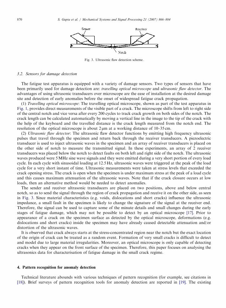
Fig. 3. Ultrasonic flaw detection scheme.

S. Gupta et al. / Mechanical Systems and Signal Processing 21 (2007) 866–884870

3.2. Sensors for damage detection

The fatigue test apparatus is equipped with a variety of damage sensors. Two types of sensors that havebeen primarily used for damage detection are: travelling optical microscope and ultrasonic flaw detector. Theadvantages of using ultrasonic transducers over microscope are the ease of installation at the desired damagesite and detection of early anomalies before the onset of widespread fatigue crack propagation.

(1) Travelling optical microscope: The travelling optical microscope, shown as part of the test apparatus inFig. 1, provides direct measurements of the visible part of a crack. The microscope shifts from left to right sideof the central notch and vice versa after every 200 cycles to track crack growth on both sides of the notch. Thecrack length can be calculated automatically by moving a vertical line in the image to the tip of the crack withthe help of the keyboard and the travelled distance is the crack length measured from the notch end. Theresolution of the optical microscope is about 2mm at a working distance of 10–35 cm.

(2) Ultrasonic flaw detector: The ultrasonic flaw detector functions by emitting high frequency ultrasonicpulses that travel through the specimen and return back through the receiver transducers. A piezoelectrictransducer is used to inject ultrasonic waves in the specimen and an array of receiver transducers is placed onthe other side of notch to measure the transmitted signal. In these experiments, an array of 2 receivertransducers was placed below the notch to detect faults on both left and right side of the notch. The ultrasonicwaves produced were 5MHz sine wave signals and they were emitted during a very short portion of every loadcycle. In each cycle with sinusoidal loading at 12.5Hz, ultrasonic waves were triggered at the peak of the loadcycle for a very short instant of time. Ultrasonic measurements were taken at stress levels that exceeded thecrack opening stress. The crack is open when the specimen is under maximum stress at the peak of a load cycleand this causes maximum attenuation of the ultrasonic waves. Note that if the crack closure occurs at lowloads, then an alternative method would be needed to detect anomalies.

The sender and receiver ultrasonic transducers are placed on two positions, above and below centralnotch, so as to send the signal through the region of crack propagation and receive it on the other side, as seenin Fig. 3. Since material characteristics (e.g. voids, dislocations and short cracks) influence the ultrasonicimpedance, a small fault in the specimen is likely to change the signature of the signal at the receiver end.Therefore, the signal can be used to capture some of the minute details and small changes during the earlystages of fatigue damage, which may not be possible to detect by an optical microscope [17]. Prior toappearance of a crack on the specimen surface as detected by the optical microscope, deformations (e.g.dislocations and short cracks) inside the specimen may have already caused detectable attenuation and/ordistortion of the ultrasonic waves.

It is observed that crack always starts at the stress-concentrated region near the notch but the exact locationof the origin of crack can be treated as a random event. Formation of very small cracks is difficult to detectand model due to large material irregularities. Moreover, an optical microscope is only capable of detectingcracks when they appear on the front surface of the specimen. Therefore, this paper focuses on analysing theultrasonics data for characterisation of fatigue damage in the small crack regime.

4. Pattern recognition for anomaly detection

Technical literature abounds with various techniques of pattern recognition (for example, see citations in[18]). Brief surveys of pattern recognition tools for anomaly detection are reported in [19]. The existing


techniques of pattern recognition, which have been used in this paper for comparison with the proposed STSAapproach, are as follows:

�
multilayer perceptron neural network (MLPNN); � radial basis function neural network (RBF); � principal component analysis (PCA).
These techniques are briefly described for completeness of the paper and in the context of their utilisation foranomaly detection.

4.1. Multilayer perceptron neural network (MLPNN)

The multilayer perceptron (MLP) neural network is a collection of connected processing elements, callednodes or neurons [19–21] whose structure is fixed by choosing the number of layers as well as the (possiblydifferent) number of neurons in each layer. The training phase includes modelling of the input–output systemarchitecture and identification of the synapsis weights. A set of inputs is passed forward through the networkyielding trial outputs which are then compared to the target outputs to obtain the error. The networkparameters (i.e. synapsis weights and biases) are adjusted until the error is within the specified bounds. If thespecified bound is exceeded, the error is passed backwards through the net and the training algorithm adjuststhe synapsis weights. The back-propagation algorithm has been used in this paper to update the networkparameters in the direction in which the performance function decreases most rapidly until the error is withinthe specified bounds. The mean square error criterion is adopted in the recursive algorithm to update theweight vectors wk as follows:

wnþ1 ¼ wn � angn, (1)

where gn is the gradient qJ=qw and an is the learning rate and J is the training error given by

JðwÞ ¼1

2

Xq

j¼1

ðoj � djÞ2, (2)

where o and d are the actual output vector and the target output vector, respectively, each ofdimension q.

Time series data of signals enter into the input layer nodes, progress forward through the hidden layers,and finally emerge from the output layer. Each node i at a given layer k receives a signal from allnodes j in its preceding layer ðk � 1Þ through a synapsis of weight wk

ij and the process is carried ontothe nodes in the following layer ðk þ 1Þ. The weighted sum of signals xk�1

j from all nodes j of thelayer ðk � 1Þ together with a bias wk

i0 produces the excitation zki that, in turn, is passed through a

non-linear activation function f to generate the output xki from the node i at the layer k. This is mathematically

expressed as

zki ¼

Xj

wkijx

k�1j þ wk

i0, ð3Þ

xki ¼ f zk

i

� �. ð4Þ

Various choices for the activation function are possible; the hyperbolic tangent function tanhð�Þ hasbeen adopted in this paper. For anomaly detection, the MLPNN is trained by setting a set of N inputvectors, each of dimension ‘, and a specified target output vector d of dimension q. This implies thatthe input layer has ‘ neurons and the output layer has q neurons. If the time series data are obtainedfrom an ergodic process, then a data set of length N ‘ can be segmented into N vectors of length ‘ toconstruct the input and target pattern matrices. The input pattern matrix P 2 R‘�N is obtained from the N

input vectors as

P � p1 p2 � � � pN� �

, (5)


where pk � yðk�1Þ‘þ1 yðk�1Þ‘þ2 � � � yk‘

h iTand each yk is a sample from the ensemble of the time series data.

The corresponding output matrix O is the output of the trained MLPNN under the input pattern P.

O � o1 o2 � � � oN� �

, (6)

where oi 2 Rq is the output of the trained MLPNN under the input pi 2 R‘. The performance vector u 2 Rq isobtained as the average of the N outputs.

u �1

N

XN

k¼1

ok. (7)

The time series data under the nominal condition generates the input pattern matrix Pnom that, in turn, is usedto train the MLPNN with respect to a target output vector d. The resulting output of the trained MLPNNwith Pnom as the input is Onom and the performance vector is unom. Subsequently, input pattern matricesfP1;P2; . . . ;Pk; . . .g are obtained at slow-time epochs ft1; t2; . . . ; tk; . . .g and corresponding output matrices ofthe trained MLPNN are fO1;O2; . . . ;Ok . . .g, which yield the respective performance vectors fu1; u2; . . . ; uk . . .g.The behavioural changes are described as anomaly from ideal condition and these anomalies are characterisedby a scalar called anomaly measure. The anomaly measure at slow-time epoch tk is obtained as

Mk � d uk; unomð Þ, (8)

where the dð�; �Þ is an appropriately defined distance function [22]. In the present analysis, the distancefunction d is chosen as the Euclidean norm and hence the anomaly measure is given by

Mk � kuk � unomk2. (9)

4.2. Radial basis function neural network (RBFNN)

In a radial basis function neural network [20], the activation of a hidden unit is determined by the distancebetween the input vector and the prototype vector. The RBFNN is essentially a nearest neighbour type ofclassifier. A radial basis function is introduced as

f ða; yÞ ¼ exp �

Pjjyj � mja

Nya

� �, (10)

where the exponent parameter a 2 ð0;1Þ; the time series y � fyjg is generated on the fast-time scale; and m andya are the centre and ath central moment of the data set, respectively. For a ¼ 2, f ð�Þ becomes Gaussian,which is the typical radial basis function used in the neural network literature. To perform anomaly detection,the first task is to obtain the sampled time series data when the dynamical system is in the nominal conditionand then the mean m and the central moment ya are calculated as

m ¼1

N

XN

j¼1

yj and ya ¼1

N

XN

j¼1

jyj � mja. (11)

The distance between any vector y and the centre m is obtained as ðPn

jyðnÞ � mjaÞ1=a. Following Eq. (10), theradial basis function at the nominal condition is f nom ¼ f ða; yÞ. Under all conditions including anomalousones, the parameters m and y are kept fixed. However, at slow-time epochs ft1; t2; . . . ; tk; . . .g, the radial basisfunctions ff 1; f 2; . . . ; f k; . . .g are evaluated from the data sets under possibly anomalous conditions. Theanomaly measure at an epoch tk in the slow-time scale is obtained as a distance from the nominal conditionand is given by

Mk ¼ dðf k; f nomÞ,

where the metric dð�; �Þ is chosen as the Euclidean distance (see Eq. (9)).


4.3. Principal component analysis (PCA)

The PCA [18,23] is the best known linear feature extractor. The eigenvectors corresponding to the q largesteigenvalues of the (n� n) (positive semi-definite) covariance matrix generated from the time series data, formthe n-dimensional patterns. The linear transformation is then defined as

Y ¼ HX , (12)

where X is the (n� d) transposed data matrix, made of n row vectors; H is the (q� n) linear transformationmatrix whose rows represent q feature vectors each of dimension n; and Y is the derived (q� d) transformeddata matrix.

To detect growth in anomaly from the time series data, principal component analysis is performed fordimensionality reduction. Data samples of large enough length (‘ ¼ n d) can be used to capture the dynamicalcharacteristics of the observed process. The length ‘ of time series data is partitioned into n subsections, eachbeing of length d ¼ ‘=n, where d4n. The resulting (d � n) data matrix is processed to generate the (n� n)covariance matrix that is positive-definite or positive-semidefinite real-symmetric. The next step is to computethe orthonormal eigenvectors v1; v2; . . . ; vn and the corresponding eigenvalues l1; l2; . . . ; ln that are arranged indecreasing orders of magnitude. The eigenvectors associated with the first (i.e. largest) q eigenvalues arechosen as the feature vectors such thatPn

i¼qþ1liPni¼1li

oZ, (13)

where the threshold Z51 is a positive real close to 0. The resulting pattern is the matrix, consisting of thefeature vectors as columns,

eM ¼ ffiffiffiffiffil1

pv1 . . .

ffiffiffiffiffilq

pvq

� . (14)

The above steps are executed for time series data under the nominal (stationary) condition to obtain eMnom.Then, these steps are repeated at subsequent slow-time epochs, ft1; t2; . . . ; tk; . . .g, using the same values ofparameters, ‘, d, n and q, to obtain the respective pattern matrices f eM1; eM2; . . . ; eMk . . .g. The anomalymeasure at a slow-time epoch tk is obtained as

Mk � d eMk; eMnom

� where the metric dð�; �Þ is chosen as the induced Euclidean norm of the matrix difference (see Eq. (9)).

5. Symbolic time series analysis (STSA)

A data sequence (e.g. time series data) can be converted to a symbol sequence by partitioning a compactregion O of the phase space, over which the trajectory evolves, into finitely many discrete blocks as shown inFig. 4. Let fF1;F2; . . . ;Fmg be a partitioning of O, such that it is exhaustive and mutually exclusive set, i.e.

[mj¼1

Fj ¼ O and Fj \ Fk ¼ ; 8jak. (15)

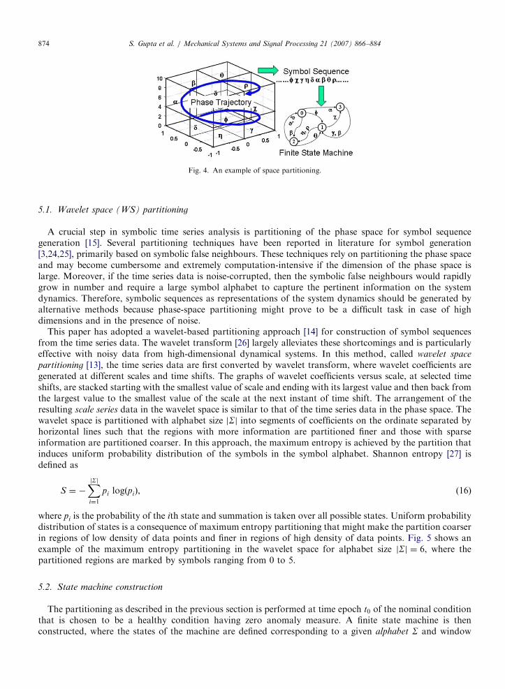
Each block Fj is labelled as the symbol sj � S, where the symbol set S is called the alphabet set consisting ofm different symbols. As the system evolves in time, it travels through various blocks in its phase space and thecorresponding symbol sj � S is assigned to it, thus converting a data sequence to a symbol sequence. . . si1si2 . . . sik . . . . Fig. 4 exemplifies the partitioning of the phase space where each block is assigned aparticular symbol such that a symbol sequence is generated from the phase space at a given slow-time epoch.Once the symbol sequence is obtained, the next step is the construction of the finite state machine. These stepsare explained in details in the following subsections.

ARTICLE IN PRESS

Fig. 4. An example of space partitioning.


5.1. Wavelet space (WS) partitioning

A crucial step in symbolic time series analysis is partitioning of the phase space for symbol sequencegeneration [15]. Several partitioning techniques have been reported in literature for symbol generation[3,24,25], primarily based on symbolic false neighbours. These techniques rely on partitioning the phase spaceand may become cumbersome and extremely computation-intensive if the dimension of the phase space islarge. Moreover, if the time series data is noise-corrupted, then the symbolic false neighbours would rapidlygrow in number and require a large symbol alphabet to capture the pertinent information on the systemdynamics. Therefore, symbolic sequences as representations of the system dynamics should be generated byalternative methods because phase-space partitioning might prove to be a difficult task in case of highdimensions and in the presence of noise.

This paper has adopted a wavelet-based partitioning approach [14] for construction of symbol sequencesfrom the time series data. The wavelet transform [26] largely alleviates these shortcomings and is particularlyeffective with noisy data from high-dimensional dynamical systems. In this method, called wavelet space

partitioning [13], the time series data are first converted by wavelet transform, where wavelet coefficients aregenerated at different scales and time shifts. The graphs of wavelet coefficients versus scale, at selected timeshifts, are stacked starting with the smallest value of scale and ending with its largest value and then back fromthe largest value to the smallest value of the scale at the next instant of time shift. The arrangement of theresulting scale series data in the wavelet space is similar to that of the time series data in the phase space. Thewavelet space is partitioned with alphabet size jSj into segments of coefficients on the ordinate separated byhorizontal lines such that the regions with more information are partitioned finer and those with sparseinformation are partitioned coarser. In this approach, the maximum entropy is achieved by the partition thatinduces uniform probability distribution of the symbols in the symbol alphabet. Shannon entropy [27] isdefined as

S ¼ �XjSji¼1

pi logðpiÞ, (16)

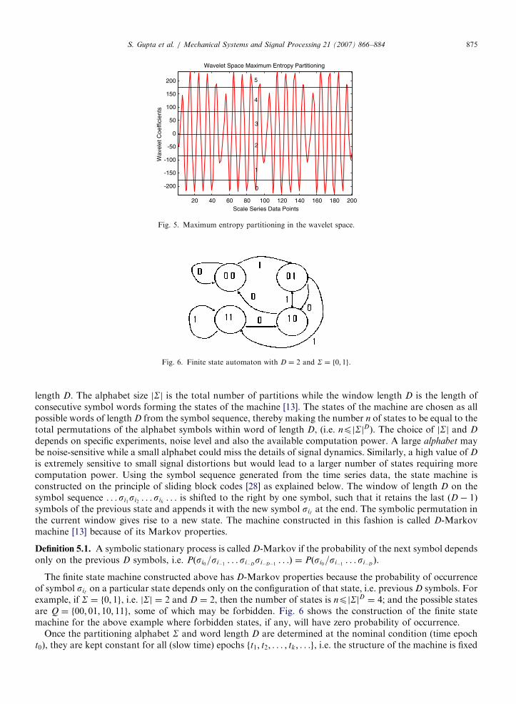
where pi is the probability of the ith state and summation is taken over all possible states. Uniform probabilitydistribution of states is a consequence of maximum entropy partitioning that might make the partition coarserin regions of low density of data points and finer in regions of high density of data points. Fig. 5 shows anexample of the maximum entropy partitioning in the wavelet space for alphabet size jSj ¼ 6, where thepartitioned regions are marked by symbols ranging from 0 to 5.

5.2. State machine construction

The partitioning as described in the previous section is performed at time epoch t0 of the nominal conditionthat is chosen to be a healthy condition having zero anomaly measure. A finite state machine is thenconstructed, where the states of the machine are defined corresponding to a given alphabet S and window

ARTICLE IN PRESS

20 40 60 80 100 120 140 160 180 200

-200

-150

-100

-50

0

50

100

150

200

Scale Series Data Points

Wav

elet

Coe

ffici

ents

Wavelet Space Maximum Entropy Partitioning

5

4

3

2

1

0

Fig. 5. Maximum entropy partitioning in the wavelet space.

Fig. 6. Finite state automaton with D ¼ 2 and S ¼ f0; 1g.


length D. The alphabet size jSj is the total number of partitions while the window length D is the length ofconsecutive symbol words forming the states of the machine [13]. The states of the machine are chosen as allpossible words of length D from the symbol sequence, thereby making the number n of states to be equal to thetotal permutations of the alphabet symbols within word of length D, (i.e. npjSjD). The choice of jSj and D

depends on specific experiments, noise level and also the available computation power. A large alphabet maybe noise-sensitive while a small alphabet could miss the details of signal dynamics. Similarly, a high value of D

is extremely sensitive to small signal distortions but would lead to a larger number of states requiring morecomputation power. Using the symbol sequence generated from the time series data, the state machine isconstructed on the principle of sliding block codes [28] as explained below. The window of length D on thesymbol sequence . . . si1si2 . . . sik

. . . is shifted to the right by one symbol, such that it retains the last ðD� 1Þsymbols of the previous state and appends it with the new symbol si‘ at the end. The symbolic permutation inthe current window gives rise to a new state. The machine constructed in this fashion is called D-Markovmachine [13] because of its Markov properties.

Definition 5.1. A symbolic stationary process is called D-Markov if the probability of the next symbol dependsonly on the previous D symbols, i.e. Pðsi0=si�1 . . . si�D

si�D�1. . .Þ ¼ Pðsi0=si�1 . . . si�D

Þ.

The finite state machine constructed above has D-Markov properties because the probability of occurrenceof symbol si‘ on a particular state depends only on the configuration of that state, i.e. previous D symbols. Forexample, if S ¼ f0; 1g, i.e. jSj ¼ 2 and D ¼ 2, then the number of states is npjSjD ¼ 4; and the possible statesare Q ¼ f00; 01; 10; 11g, some of which may be forbidden. Fig. 6 shows the construction of the finite statemachine for the above example where forbidden states, if any, will have zero probability of occurrence.

Once the partitioning alphabet S and word length D are determined at the nominal condition (time epocht0), they are kept constant for all (slow time) epochs ft1; t2; . . . ; tk; . . .g, i.e. the structure of the machine is fixed


at the nominal condition. That is, the partitioning and the state machine structure, generated at the nominalcondition serve as the reference frame for data analysis at subsequent time epochs.

In this analysis, it was found that the combination of jSj ¼ 8 and D ¼ 1 was able to capture anomaliesearlier than the optical microscope. For D ¼ 1, the set of states bears an equivalence relation to the alphabet Sof symbols [22]. The states of the machine are marked with the corresponding symbolic word permutation andthe edges joining the states indicate the occurrence of an event si‘ . The occurrence of an event at a state maykeep the machine in the same state or move it to a new state. The language of the machine is usuallyincomplete in the sense that all states might not be reachable from a given state.

Definition 5.2. The probability of transitions from state qj to state qk belonging to the set Q of states under atransition d : Q� S! Q is defined as

pjk ¼ Pðs 2 S j dðqj ;sÞ ! qkÞ;X

k

pjk ¼ 1. (17)

Thus, for a D-Markov machine, the irreducible stochastic matrix P � pij

� �describes all transition

probabilities between states such that it has at most jSjDþ1 non-zero entries. The left eigenvector p

corresponding to the unit eigenvalue of P is the state probability vector under the (fast time scale) stationarycondition of the dynamical system [13]. On a given symbol sequence . . . si1si2 . . . sil

. . . generated from the timeseries data collected at slow-time epoch tk, a window of length (D) is moved by keeping a count of occurrencesof word sequences si1 � � � siD

siDþ1and si1 � � � siD

which are, respectively, denoted by Nðsi1 � � � siDsiDþ1Þ and

Nðsi1 � � � siDÞ. Note that if Nðsi1 � � � siD

Þ ¼ 0, then the state q � si1 � � �siD 2 Q has zero probability ofoccurrence. For Nðsi1 � � �siD Þa0, the transitions probabilities are then obtained by these frequency counts asfollows:

pjk ¼Pðsi1 � � �siD

sÞPðsi1 � � � siD

Þ�

Nðsi1 � � �siDsÞ

Nðsi1 � � � siDÞ, (18)

where the corresponding states are denoted by qj � si1si2 � � �siD and qk � si2 � � � siDs.

The time series data under the nominal condition (set as a benchmark) generates the state transition matrix

Pnom that, in turn, is used to obtain the state probability vector pnom whose elements are the stationaryprobabilities of the state vector, where pnom is the left eigenvector of Pnom corresponding to the (unique) uniteigenvalue. Subsequently, state probability vectors p1; p2; . . . ; pk; . . . are obtained at slow-time epochst1; t2; . . . ; tk; . . . based on the respective time series data. Machine structure and partitioning should be thesame at all slow-time epochs.

The anomaly measure at slow-time epochs tk is obtained as

Mk � d pk; pnom� �

, (19)

where the dð�; �Þ is chosen as the Euclidean norm of the vector difference (see Eq. (9)).

5.3. Summary of STSA anomaly detection

The following steps summarise the procedure of anomaly detection using symbolic time series analysis(STSA).

�
Collection of time series data from appropriate sensor(s) at time epoch t0 of the nominal condition, wherethe system is assumed to be in the healthy state (i.e. zero anomaly measure). � Stacking of the wavelet transform coefficients (obtained with an appropriate choice of mother wavelet andrange of scales) that are generated from the time series data at time epoch t0 to generate the scale series data(see Section 5.1). � Partitioning of the scale series data into jSj regions using maximum Entropy partitioning to obtain thesymbol sequence. � Construction of the D-Markov machine states from the chosen alphabet size jSj and the window length D
and generation of the state probability vector p0 at time epoch t0 of the nominal condition.


�
Generation of time series data sequences at subsequent slow-time epochs, t1; t2; . . . ; tk; . . . , and theirconversion to the scale series data in the wavelet domain to generate respective symbolic sequences using thepartitioning at time epoch t0 of the nominal condition. � Generation of the state probability vectors at slow-time epochs, t1; t2; . . . ; tk; . . . from the respective symbolicsequences using the finite state machine at time epoch t0 of the nominal condition. � Computation of the anomaly measures at time epochs, t1; t2; . . . ; tk; . . . relative to the probability vector attime epoch t0 of the nominal condition.
5.4. Real time application

Fatigue damage detection using STSA has been implemented in real time. However, the results presented inthis paper are generated by off-line analysis. For real time application, the same steps have been followed asdescribed in the previous sections. The nominal condition is chosen after the start of the experiment at a timeepoch t0 where the system attains the steady state and is assumed to be in the healthy condition with zeroanomaly measure. The machine states are fixed in advance using a priori determined values of the parameters:alphabet size jSj and window length D. The partitioning and machine construction were performed based onthe time series data at the slow-time epoch t0 and the resulting information (i.e. partitioning data and the stateprobability vector at this nominal condition) was stored for future computation of anomaly measures at futureslow-time epochs, t1; t2; . . . ; tk; . . . ; that were separated by uniform intervals of time in these experiments. Thetime series data of ultrasonic sensor signals were written as text files so that the STSA algorithm could read thedata from the text files to calculate the anomaly measure at those time epochs. The algorithm iscomputationally very fast and the results can be plotted on the screen such that the plot updates itself with themost recent anomaly measure at that particular time epoch. This procedure allows on-line health monitoringat any time and is capable of issuing early warnings.

6. Experimental data collection and analysis

The fatigue tests were conducted using specimens, made of the aluminium alloy 7075-T6, at a constantamplitude sinusoidal load for a low-cycle fatigue, where the maximum and minimum loads were kept constantat 87 and 4.85MPa. (see Section 3 for a description of the test apparatus.) For low-cycle fatigue, the stressamplitude at the crack tip is sufficiently high to observe the elasto-plastic behaviour in the specimens undercyclic loading. A significant amount of internal damage occurs before the crack appears on the surface of thespecimen when it is observed by the microscope. This internal damage caused by multiple small cracks,dislocations and microstructural damage affects the ultrasonic waves when they pass through the region wherethese faults have developed. This phenomenon causes signal distortion and attenuation at the receiver end.The crack propagation stage starts when this internal damage eventually develops into a single large crack.Subsequently, the crack growth rate increases rapidly and when the crack is sufficiently large, completeattenuation of the transmitted ultrasonic signal occurs, as seen at the receiver end.

6.1. Ultrasonic and optical image data collection

The ultrasonic sensing device was triggered at a frequency of 5MHz at each peak of the ð�12:5HzÞsinusoidal load to obtain 100 data points in each cycle. Since the ultrasonic frequency is much higher than theload frequency, the data collection was performed for a very short interval in the time scale of loadfluctuations. Therefore, it can be implied that the ultrasonic data were collected at the peak of each sinusoidalload cycle, where the stress is maximum and the crack is open causing maximum attenuation of the ultrasonicwaves. The slow-time epochs were chosen to be 3000 load cycles (i.e. �240 s) apart. At the onset of each slow-time epoch, the ultrasonic data points were collected on the fast time scale of 100 cycles (i.e. �8 s), whichproduced a string of 10 000 data points. At a frequency of 12.5Hz, 100 cycles take only 8 s to run and it isassumed that during this fast time scale of 100 cycles, the system remained in a stationary condition and nomajor changes occurred in the fatigue crack behaviour. This set of time series data collected in the manner


described above at different slow-time epochs was analysed by several techniques to calculate anomalymeasures at those slow-time epochs.

The optical images were collected at every 200 cycles until a crack was detected on the specimen surface bythe optical microscope. Then onwards the images were taken at user command and the microscope was movedsuch that it always focused on the crack tip. The vertical line in the images was adjusted by the movement ofthe microscope until it reached the crack tip. The distance travelled by the microscope determined the cracklength.

The nominal condition at the slow-time epoch t0 was chosen to be 5 kilocycles to ensure that the electro-hydraulic system of the test apparatus had come to a steady state and that no significant damage occurred tillthat point. This nominal condition was chosen as a benchmark where the specimen was assumed to be in ahealthy state, where the anomaly measure was chosen to be zero. The anomalies at subsequent slow-timeepochs, t1; t2; . . . ; tk; . . . , were then calculated with respect to the nominal condition at t0. It is emphasised thatthe anomaly measure is relative to the nominal condition which is fixed in advance and should not be confusedwith the actual damage at an absolute level. Any particular value of the anomaly measure greater than zeroindicates deviation from the nominal condition and it signifies that some changes have occurred inside thespecimen.

6.2. Data analysis and damage evaluation

This section evaluates the collected time series data for early detection of anomalies resulting from fatiguedamage. The proposed anomaly detection technique is compared with other pattern recognition tools (seeSection 4).

(1) MLPNN : Following the MLPNN procedure, described in Section 4.1, the input pattern matrix Pnom

was designed with N ¼ 200 columns. Each column, having a length of ‘ ¼ 50, was generated from theultrasonic data collected at the nominal condition at time instant t0 to train the MLPNN. The neural networkwas designed with an input layer (with 50 neurons), 3 hidden layers (with 40 neurons in layer 1, 30 neurons inlayer 2 and 40 neurons in layer 3) and the output layer (with 10 neurons). The target corresponding to eachinput pattern vector was chosen to be the 10� 1 zero vector. The gradient descent back-propagationalgorithm was used for network training with an allowable performance mean square error of 1:0� 10�5. Theinput pattern matrices P1;P2; . . . ; Pk; . . . , each of dimension ð50� 200Þ, were then generated from theanomalous data sets at slow-time epochs ft1; t2; . . . ; tk; . . .g . Anomaly measures were then calculated with theprocedure described in Section 4.1.

(2) RBF: Following the RBF procedure for anomaly detection as described in Section 4.2, the standard RBFwas chosen with the exponent a to be equal to 2. Lower values of alpha reduced anomaly measure sensitivityand higher values of alpha produced noisy results. An estimate of the parameters, m and ya, were obtainedaccording to Eq. (11) based on the data under the nominal condition at t0, which produced the requisite radialbasis function f nom following Eq. (10). At slow-time epochs ft1; t2; . . . ; tk; . . .g the radial basis functionsff 1; f 2; . . . ; f k; . . .g were evaluated from the data sets collected at those time epochs. Anomaly measures werethen calculated with the procedure described in Section 4.2.

(3) PCA: Following the PCA procedure for anomaly detection as described in Section 4.3, a block ofsampled ultrasonic data, having length of 10 000, was divided into n ¼ 8 segments, each of which was of length‘ ¼ 1250; these segments were then arranged to form a 1250� 8 data matrix. The resulting 8� 8 (symmetricpositive-definite) covariance matrix of the data matrix provided a monotonically decreasing set of eigenvalues,l1; . . . ; l8, and the associated orthonormal eigenvectors v1; . . . ; v8. At time instant t0 of the nominal condition,the first eigenvalue was found to be the dominant (i.e. q ¼ 1) for a threshold of Z ¼ 0:05 such thatP8

i¼2liP8i¼1li

oZ.

The pattern matrix eMnom was generated at the nominal condition t0 and the pattern matriceseM1; eM2; . . . ; eMk; . . . were generated at time instants t1; t2; . . . ; tk; . . . . Anomaly measures were then calculatedfollowing the procedure described in section 4.3.


(4) STSA: Following the STSA procedure for anomaly detection as described in Section 5, the alphabet sizefor partitioning was chosen to be jSj ¼ 8 and window length of D ¼ 1, while the mother wavelet chosen to be‘gaus2’ [29]. (Absolute values of the wavelet scale series data were used to generate the partition because of thesymmetry of the data sets about their mean.) This combination of parameters was capable of capturing theanomalies earlier than the optical microscope. Increasing the value of jSj further did not improve the resultsand increasing the value of D created a large number of states of the finite state machine, many of them havingvery small or zero probabilities, and required larger number of data points at each time epoch to stabilise thestate probability vectors. This choice of the parameters jSj and D was able to capture early anomalies withonly 8 states and was computationally very fast in the sense that the code execution time was orders ofmagnitude smaller than the process response time. The mother wavelet of ‘gaus2’ provided better results thanmany other wavelets of the Daubechies family [26] because it closely matched the shape of the sinusoidalsignals. State Probability vector pnom was obtained at the nominal condition of time epoch t0 and the stateprobability vectors p1; p2; . . . ; pk; . . . were obtained at other slow-time epochs t1; t2; . . . ; tk; . . . . Anomalymeasures were calculated with the procedure described in Section 5.

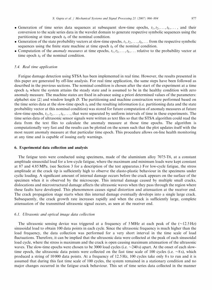
The six pairs of plates in Fig. 7 show two-dimensional images of a specimen surface and histograms ofprobability distribution of automaton states at six different time epochs, approximately 5, 30, 40, 45, 60 and 78kilocycles, exhibiting gradual evolution of fatigue damage. In each pair of plates from (a)–(f) in Fig. 7, the topplate exhibits the surface image of the test specimen as seen by the optical microscope. As exhibited on the topplates in each of the six plate pairs in Fig. 7, the crack originated and developed on the right side of the notch

Fig. 7. Pictorial view of crack damage and corresponding probability distribution.


at the centre. Histograms in the bottom plates of six plate pairs in Fig. 7 show the evolution of the stateprobability vector corresponding to fatigue damage growth on the test specimen at different slow-time epochs,signifying how the probability distribution gradually changes from uniform distribution (i.e. minimalinformation) to delta distribution (i.e. maximum information).

The top plate in plate pair (a) of Fig. 7 shows the image at the nominal condition ð�5 kilocyclesÞ when theanomaly measure is taken to be zero, which is considered as the reference point with the available informationon potential damage being minimal. This is reflected in the uniform distribution (i.e. maximum entropy) asseen from the histogram at the bottom plate of plate pair (a).

Both the top plates in plate pairs (b) and (c) at �30 and �40 kilocycles, respectively, do not yet have anyindication of surface crack although the corresponding bottom plates do exhibit deviations from the uniformprobability distribution (see the bottom plate of plate pair (a)). This is an evidence that the analyticalmeasurements, based on ultrasonic sensor data, produce damage information during crack initiation, which isnot available from the corresponding optical images.

The top plate in plate pair (d) of Fig. 7 at �45 kilocycles exhibits the first noticeable appearance of a�300 mm crack on the specimen surface, which may be considered as the boundary of the crack initiation andpropagation phases. This small surface crack indicates that a significant portion of the crack or multiple smallcracks might have already developed underneath the surface before they started spreading on the surface. Thehistogram of probability distribution in the corresponding bottom plate shows further deviation from theuniform distribution at �5 kilocycles. This is also an indication of having increasingly more information ondamage than what was available in the earlier cycles.

The top plate in plate pair (e) of Fig. 7 at �60 kilocycles exhibits a fully developed crack in its propagationphase. The corresponding bottom plate shows the histogram of the probability distribution that is significantlydifferent from those in earlier cycles in plate pairs (a)–(d), indicating further gain in the information on crackdamage. The top plate in plate pair (f) of Fig. 7 at �78 kilocycles exhibits the image of a completely brokenspecimen. The corresponding bottom plate shows delta distribution indicating complete information on crackdamage.

The observation in Fig. 7 is further clarified by using the notion of entropy (see Eq. (16)). The scale seriesdata at the nominal condition were partitioned using the maximum entropy principle, which led to uniformprobability distribution (i.e. maximum entropy) among the states in the bottom plate of plate pair (a) in Fig. 7.In contrast, for the completely broken stage of the specimen, the entire probability distribution is concentratedin only one state of the finite state machine as seen in the bottom plate of plate pair (f) in Fig. 7, whichindicates a very large attenuation of the ultrasonic signal. This phenomenon of the sample being completelybroken signifies certainty of information and hence zero entropy. Therefore, as the fatigue crack damageevolves, the uniform distribution (i.e. maximum entropy) under nominal condition degenerates toward thedelta distribution (i.e. zero entropy) for the broken specimen. In the intermediate stages, gradual degradationcan be quantitatively evaluated using this information. Fig. 8 shows the monotonically decreasing profile ofentropy versus load cycles, which is a clear evidence of gradual evolution of fatigue crack damage with loadcycles. The sharp decrease in entropy from the first appearance of a surface crack at �45 kilocycles to thecomplete breakage at �78 kilocycles can be related to phase transition of first order in the thermodynamicsense [30].

6.3. Comparative evaluation of damage detection techniques

This section makes a comparative assessment of the proposed STSA method with other existing techniquesof pattern recognition, described in Section 4 for early detection of fatigue crack damage using the ultrasonicsensor data generated on the test apparatus described in Section 3. The following anomaly detectionapproaches were investigated.

�
multilayer perceptron neural network (MLPNN); � radial basis function neural network (RBFNN); � principal component analysis (PCA); � symbolic time series analysis (STSA).

ARTICLE IN PRESS

0 10 20 30 40 50 60 70 800

0.1

0.2

0.3

0.4

0.5

0.6

0.7

0.8

0.9

1

Load Kilocycles

Nor

mal

ized

Ano

mal

y M

easu

re

PCARBFMLPNNSTSA

First CrackDetection byMicroscope

Fig. 9. Performance comparison for fatigue damage detection.

0 10 20 30 40 50 60 70 800

0.1

0.2

0.3

0.4

0.5

0.6

0.7

0.8

0.9

1

Load Kilocycles

Nor

mal

ized

Ent

ropy

Nominal Condition

Crack Appearance

Crack Propagation

Broken Specimen

Fig. 8. Evolution of entropy with fatigue damage growth.


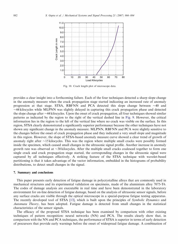
The efficacy of a specific approach is largely determined by its capability for early detection of smallanomalies. The four plots in Fig. 9 compare the anomaly measures obtained by using the afore-described fouranomaly detection approaches. Each of the curves in Fig. 9 show a possible bifurcation where the slope of theanomaly measure changes dramatically indicating the onset of crack propagation phase. First appearance offatigue crack was detected by the optical microscope at approximately 45 kilocycles, which is marked by thedashed vertical line in Fig. 9. The crack when it appeared on the surface was �300mm long, which implies thata significant amount of fatigue damage including multiple small cracks developed inside the specimen beforethey finally spread out to the surface. Fig. 10 shows the fatigue crack growth in millimeters vs the load cycles,which was derived from the optical images.

A comparison of the plots in Fig. 9 clearly indicates that the STSA technique for anomaly detection yieldedthe best performance among all methods. It is observed that small changes can be detected by STSAsignificantly before the microscope can capture a surface crack. The slope of the anomaly measure representsthe anomaly growth rate while the magnitude indicates the changes that have occurred relative to the nominalcondition. An abrupt change in the slope (i.e. a sharp change in the curvature) of anomaly measure profile

ARTICLE IN PRESS

0 10 20 30 40 50 60 70 80

1.0

2.0

3.0

4.0

5.0

6.0

7.0

8.0

9.0

10.0

11.0

Cra

ck L

engt

h in

mm

Load Kilocycles

Fig. 10. Crack length plot of microscope data.


provides a clear insight into a forthcoming failure. Each of the four techniques detected a sharp slope changein the anomaly measure when the crack propagation stage started indicating an increased rate of anomalyprogression at that stage. STSA, RBFNN and PCA detected this slope change between �40 and�44 kilocycles while MLPNN was slightly delayed in capturing this crack propagation phase and detectedthe slope change after �44 kilocycles. Upon the onset of crack propagation, all four techniques showed similarpatterns as indicated by the region to the right of the vertical dashed line in Fig. 9. However, the criticalinformation lies in the region to the left of the vertical line where no crack was visible on the surface. In thisregion, STSA clearly demonstrated a significantly superior performance because the other techniques have notshown any significant change in the anomaly measure. MLPNN, RBFNN and PCA were slightly sensitive tothe changes before the onset of crack propagation phase and they indicated a very small slope and magnitudein this region. However, the slope of STSA-based anomaly measure curve showed a clear trend of growth ofanomaly right after �15 kilocycles. This was the region where multiple small cracks were possibly formedinside the specimen, which caused small changes in the ultrasonic signal profile. Another increase in anomalygrowth rate was observed at �30 kilocycles. After the multiple small cracks coalesced together to form onesingle crack and crack propagation stage started, the corresponding changes in the ultrasonic signal werecaptured by all techniques effectively. A striking feature of the STSA technique with wavelet-basedpartitioning is that it takes advantage of the vector information, embedded in the histograms of probabilitydistributions, to detect small changes in the signal.

7. Summary and conclusions

This paper presents early detection of fatigue damage in polycrystalline alloys that are commonly used inmechanical structures and its experimental validation on specimens, made of the aluminium alloy 7075-T6.The codes of damage analysis are executable in real time and have been demonstrated in the laboratoryenvironment for on-line detection of fatigue damage, based on the analysis of ultrasonic sensor signals, beforeany surface cracks are visible through the optical microscope in a special-purpose fatigue testing apparatus.The recently developed tool of STSA [13], which is built upon the principles of Symbolic Dynamics andAutomata Theory, has been adopted. Fatigue damage is detected from small changes in the statisticalcharacteristics of the sensor signals.

The efficacy of the proposed STSA technique has been examined by comparison with other existingtechniques of pattern recognition: neural networks (NN) and PCA. The results clearly show that, incomparison with the NN and PCA techniques, the performance of STSA is superior in terms of early detectionof precursors that provide early warnings before the onset of widespread fatigue damage. A combination of


maximum-entropy partitioning in the wavelet domain and symbolic dynamics was able to detect fatiguedamage growth significantly before the onset of crack propagation phase and yielded better performance thanother techniques.

The reported work is a step toward building a reliable instrumentation system for early detection of fatiguedamage in polycrystalline alloys; further research is necessary before its usage in industry. The utilisation ofthis information provided by the anomaly measure for appropriate control action for damage mitigation is anarea of future work and would require stochastic analysis of multiple data sets generated under identicalloading and environmental conditions. While there are many research issues that need to be addressed, thefollowing research topics are being currently pursued.

�
Solution of the inverse problem using ultrasonic stochastic data and development of performance boundsfor safe reliable operation. � Statistical analysis of time series data of fatigue damage, collected under identical loading andenvironmental conditions, to account for manufacturing and material uncertainties. � Validation of the STSA technique for early detection of fatigue damage under different conditions, such ashigh-cycle loading, variable-amplitude block loading, and spectral loading [31]. � Interpretation of phase changes in the fatigue damage evolution in terms of those in statistical mechanics.
Acknowledgements

The authors wish to thank their colleague Dr. S. Chin for providing useful information in generating theresults.

References

[1] S. Ozekici, Reliability and Maintenance of Complex Systems, vol. 154, NATO Advanced Science Institutes (ASI) Series F: Computer

and Systems Sciences, Berlin, Germany, 1996.

[2] K. Sobczyk, B.F. Spencer, Random Fatigue: Data to Theory, Academic Press, Boston, MA, 1992.

[3] H.D.I. Abarbanel, The Analysis of Observed Chaotic Data, Springer, New York, 1996.

[4] D.A. Cook, Y.H. Berthelot, Detection of small surface-breaking fatigue cracks in steel using scattering of Rayleigh waves, NDT&E

International 34 (2001) 483–492.

[5] S.I. Rokhlin, J.-Y. Kim, In situ ultrasonic monitoring of surface fatigue crack initiation and growth from surface cavity, International

Journal of Fatigue 25 (2003) 41–49.

[6] S. Grondel, C. Delebarre, J. Assaad, J.P. Dupuis, L. Reithler, Fatigue crack monitoring of riveted aluminium strap joints by lamb

wave analysis and acoustic emission measurement techniques, NDT&E International 35 (2002) 137–146.

[7] H. Sohn, C.R. Farrar, N.F. Hunter, K. Wordan, Structural health monitoring using statistical pattern recognition techniques,

Journal of Dynamic Systems, Measurement and Control 123 (December 2001) 706–711.

[8] Z.K. Peng, F.L. Chu, Application of the wavelet transform in machine condition monitoring and fault diagnosis: a review with

bibliography, Mechanical Systems and Signal Processing 18 (2004) 199–221.

[9] X. Lou, K.A. Loparo, Bearing fault diagnosis based on wavelet transform and fuzzy interference, Mechanical Systems and Signal

Processing 18 (2004) 1077–1095.

[10] J.M. Nichols, M.D. Todd, M. Seaver, L.N. Virgin, Use of chaotic excitation and attractor property analysis in structural health

monitoring, Physical Review E 67 (016209) (2003).

[11] W.J. Wang, J. Chen, X.K. Wu, Z.T. Wu, The application of some non-linear methods in rotating machinery fault diagnosis,

Mechanical Systems and Signal Processing 15 (4) (2001) 697–705.

[12] L. Moniz, J.M. Nichols, C.J. Nichols, M. Seaver, S.T. Trickey, M.D. Todd, L.M. Pecora, L.N. Virgin, A multivariate, attractor-

based approach to structural health monitoring, Journal of Sound and Vibration Processing 283 (2005) 295–310.

[13] A. Ray, Symbolic dynamic analysis of complex systems for anomaly detection, Signal Processing 84 (7) (2004) 1115–1130.

[14] V. Rajagopalan, A. Ray, Wavelet-based space partitioning for symbolic time series analysis, Proceedings of 44th IEEE Conference on

Decision and Control and European Control Conference, Seville, Spain, December 2005.

[15] C.S. Daw, C.E.A. Finney, E.R. Tracy, A review of symbolic analysis of experimental data, Review of Scientific Instruments 74 (2)

(2003) 915–930.

[16] E.E. Keller, Real time sensing of fatigue crack damage for information-based decision and control, Ph.D. Thesis, Department of

Mechanical Engineering, Pennsylvania State University, State College, PA, 2001.

[17] E.E. Keller, A. Ray, Real time health monitoring of mechanical structures, Structural Health Monitoring 2 (3) (2003) 191–203.

[18] R. Duda, P. Hart, D. Stork, Pattern Classification, Wiley, New York, 2001.


[19] M. Markou, S. Singh, Novelty detection: a review—parts 1 and 2, Signal Processing 83 (2003) 2481–2521.

[20] C.M. Bishop, Neural Networks for Pattern Recognition, Oxford University Press Inc., New York, 1995.

[21] S. Haykin, Neural Networks: A Comprehensive Foundation, Prentice Hall, Upper Saddle River, NJ, 1999.

[22] A.W. Naylor, G.R. Sell, Linear Operator Theory in Engineering and Science, Springer, New York, 1982.

[23] D.P. Fukunaga, Statistical Pattern Recognition, second ed., Academic Press, Boston, 1990.

[24] R.L. Davidchack, Y.C. Lai, E.M. Bolt, H. Dhamala, Estimating generating partitions of chaotic systems by unstable periodic orbits,

Physical Review E 61 (2000) 1353–1356.

[25] M.B. Kennel, M. Buhl, Estimating good discrete partitions form observed data: symbolic false nearest neighbors, Physical Review E

91 (8) (2003) 084102.

[26] S. Mallat, A Wavelet Tour of Signal Processing 2=e, Academic Press, New York, 1998.

[27] T.M. Cover, J.A. Thomas, Elements of Information Theory, Wiley, New York, 1991.

[28] D. Lind, M. Marcus, An Introduction to Symbolic Dynamics and Coding, Cambridge University Press, Cambridge, UK, 1995.

[29] Wavelet Toolbox, MATLAB, Mathworks Inc.

[30] N. Goldenfeld, Lectures on Phase Transitions and the Renormalization Group, Perseus Books, Reading, MA, 1992.

[31] S. Gupta, A. Ray, E. Keller, Online detection of fatigue failure via symbolic time series analysis, American Control Conference,

Portland, OR, June 2005, pp. 3309–3314.

symbolic time series analysis of ultrasonic data for early

Documents