symbolic optimization with smt solvers - uw …pages.cs.wisc.edu/~aws/papers/popl14.pdf · symbolic...
TRANSCRIPT

Symbolic Optimization with SMT Solvers
Yi LiUniversity of [email protected]
Aws AlbarghouthiUniversity of [email protected]
Zachary KincaidUniversity of Toronto
Arie GurfinkelSoftware Engineering Institute, CMU
Marsha ChechikUniversity of Toronto
AbstractThe rise in efficiency of Satisfiability Modulo Theories (SMT)solvers has created numerous uses for them in software verification,program synthesis, functional programming, refinement types, etc.In all of these applications, SMT solvers are used for generatingsatisfying assignments (e.g., a witness for a bug) or proving un-satisfiability/validity (e.g., proving that a subtyping relation holds).We are often interested in finding not just an arbitrary satisfyingassignment, but one that optimizes (minimizes/maximizes) certaincriteria. For example, we might be interested in detecting programexecutions that maximize energy usage (performance bugs), or syn-thesizing short programs that do not make expensive API calls. Un-fortunately, none of the available SMT solvers offer such optimiza-tion capabilities.
In this paper, we present SYMBA, an efficient SMT-based op-timization algorithm for objective functions in the theory of linearreal arithmetic (LRA). Given a formula ϕ and an objective functiont, SYMBA finds a satisfying assignment of ϕ that maximizes thevalue of t. SYMBA utilizes efficient SMT solvers as black boxes.As a result, it is easy to implement and it directly benefits fromfuture advances in SMT solvers. Moreover, SYMBA can optimizea set of objective functions, reusing information between them tospeed up the analysis. We have implemented SYMBA and evaluatedit on a large number of optimization benchmarks drawn from pro-gram analysis tasks. Our results indicate the power and efficiency ofSYMBA in comparison with competing approaches, and highlightthe importance of its multi-objective-function feature.
Categories and Subject Descriptors G.1.6 [Optimization]: Con-strained optimization; F.3.1 [Specifying and Verifying and Rea-soning about Programs]: Invariants
Keywords optimization; satisfiability modulo theories; invariantgeneration; symbolic abstraction; program analysis
Permission to make digital or hard copies of all or part of this work for personal orclassroom use is granted without fee provided that copies are not made or distributedfor profit or commercial advantage and that copies bear this notice and the full citationon the first page. Copyrights for components of this work owned by others than ACMmust be honored. Abstracting with credit is permitted. To copy otherwise, or republish,to post on servers or to redistribute to lists, requires prior specific permission and/or afee. Request permissions from [email protected] ’14, January 22–24, 2014, San Diego, CA, USA.Copyright c© 2014 ACM 978-1-4503-2544-8/14/01. . . $15.00.http://dx.doi.org/10.1145/2535838.2535857
1. IntroductionOver the past decade or so, we have witnessed an incredible im-provement in the performance of Satisfiability Modulo Theories(SMT) solvers [10] and the range of logical theories they support.These advances made SMT solvers (e.g., Z3 [22], MathSAT [18],CVC [9], etc.) household names in the programming languages andverification communities, creating an explosion in the range of ap-plications in which they are deployed, and paving the way for in-novations that would not have been possible otherwise.
To mention a few, in verification, SMT solvers have been usedfor device driver verification [7, 35], checking complex verifica-tion conditions [23, 39, 49], and improving precision of invariantgeneration [34, 46]; in testing and bug finding, they have been in-strumental in making symbolic execution [15, 27], fuzzing [28],and bounded model checking techniques [19, 25] practical; in pro-gram synthesis, they have been used to search for programs satisfy-ing a given specification [31, 59]; in functional programming, theyhave been used to support strong typing guarantees with refinementtypes [13, 53].
In all of the aforementioned applications, SMT solvers are usedfor (1) generating satisfying assignments (e.g., a witness for a bug)or (2) proving unsatisfiability/validity (e.g., proving that a subtyp-ing relation holds). To the best of our knowledge, none of the avail-able SMT solvers support finding optimal satisfying assignments,i.e., satisfying assignments that minimize (or maximize) a givenobjective function. In this paper, we present SYMBA, an efficientSMT-based optimization algorithm for objective functions in thetheory of linear real arithmetic (LRA). Given a formula ϕ and anobjective function t, e.g., x + y, SYMBA computes the smallestconstant k such that ϕ ⇒ t 6 k 1. Specifically, SYMBA finds asatisfying assignment of ϕ that exhibits the least upper bound k(maximum value) of an objective function t. In what follows, westart by arguing that such an algorithm has a wide array of appli-cations in verification, bug finding, synthesis, and others. We thenhighlight SYMBA’s salient features and describe its high-level op-eration.
Applications of Optimization We start by describing potentialapplications of SYMBA in the following domains:
• Numerical invariant generation: Numerical abstract domains,e.g., intervals [20] and octagons [42], are often used to generatenumerical program invariants. The main ingredient in such ananalysis is the abstract transformer: an operator that takes a setof initial states and an instruction (or a basic block), and com-
1 Note that k is∞ if t is unbounded in ϕ, and −∞ if ϕ is unsatisfiable

putes a set of reachable states, often using convex optimizationtechniques. Since SYMBA can optimize over arbitrary LRA for-mulas (non-convex optimization), it can precisely compute ab-stract transformers over loop-free program fragments (encodedas formulas), without losing precision due to join or multipleapplications of the transformer. This problem is known in theliterature as symbolic abstraction and has been studied for anumber of domains [45, 46, 52, 60, 61]. By designing optimiza-tion algorithms that exploit the power of SMT solvers, we en-able efficient implementations of precise abstract transformersfor a variety of numerical domains [55]. We discuss this appli-cation in more detail in Sec. 4, where we generate our bench-mark suite from symbolic abstraction queries made by a pro-gram analysis tool [5].A similar approach can be used for solving systems of Horn-likeclauses in LRA [30, 32], which capture a large number of se-quential and concurrent program verification tasks. Since Hornclauses are represented symbolically in SMT-LIB [14], apply-ing traditional numerical abstract domains for solving them isnot a straightforward endeavour, but SYMBA can be easily usedto build a fixpoint solver for such clauses.• Counterexample generation: In symbolic execution and bounded
model checking, program executions are encoded succinctly asa formula. An SMT solver is then used to find a satisfying as-signment of this formula that acts as a witness of an erroneousexecution. By augmenting the encoding with arithmetic costfunctions, we can use SYMBA to find counterexamples thatmaximize or minimize certain criteria. For example, we mightbe interested in finding performance bugs, e.g., execution traceswith the highest energy or memory consumption. By assigningcosts to program instructions and API calls, we can detect suchexecutions using an optimizing SMT solver.• Program synthesis: Program synthesis involves generating
a program that satisfies a given specification. For example,in [31, 37], non-trivial bit-manipulating program snippets aresynthesized from specifications by using SMT solvers to searchthrough all possible combinations of bit-level operations (in-structions). Similar to the counterexample generation describedabove, the goal is often to synthesize the shortest programs, orones with the smallest cost. For example, when the synthesizedsnippet is part of a performance-critical code (e.g., as in su-peroptimization [41]), the size of the synthesized snippet andthe operations it performs are crucial. By augmenting formu-las given to the SMT solver with costs, we can instruct it tosynthesize programs that minimize a given criterion.• Constraint programming: In recent work [38], Koksal et al.
proposed incorporating an SMT solver into an extension ofScala, allowing constraint manipulation as part of the language.One of the important constructs in their language is min/max,which returns the minimum/maximum satisfying assignmentof a constraint w.r.t to an objective function, and enables ele-gant implementations of algorithms for problems like knapsack.Due to the unavailability of off-the-shelf solvers with an opti-mization feature, the authors use a simple binary search opti-mization algorithm restricted to bounded discrete domains. Theauthors of [38] also comment on the state-of-the-art of SMTsolvers by saying: “...we found that a number of features, ifnatively supported by solvers, could directly bring benefits toconstraint programming. These include 1) support for enumer-ation of theory models and 2) solving constraints while mini-mizing/maximizing a given term.” SYMBA is thus an answer topoint 2 for LRA terms (objective functions).
• Interpolant generation: Craig interpolation has proved to be apowerful technique for software verification based on predicateabstraction [36]. Interpolants are generated from unsatisfiabil-ity proofs. For linear real arithmetic, this can be performed byconstructing a system of constraints whose solution is a proof ofunsatisfiability (and an interpolant) [54]. As recently shown [4],the simplicity of the proof can be crucial to discovering thepredicates required for a safe inductive invariant. Finding sim-ple proofs boils down to finding an optimal solution of the sys-tem of constraints. Using SYMBA, this can be automated, with-out the need for the heuristics employed in [4].
Symbolic Optimization with SYMBA Given a formula ϕ and aset of objective functions (objectives for short) T = {t1, . . . , tn},SYMBA computes the strongest formula
optT (ϕ) ≡ t1 6 k1 ∧ . . . ∧ tn 6 kn,
such that ϕ ⇒ optT (ϕ), where ki ∈ R ∪ {∞,−∞}. We calloptT (ϕ) the optimal solution of T w.r.t. ϕ. In other words, SYMBAcomputes the least upper bound (maximum value) ki of each ob-jective ti w.r.t. the satisfying assignments of ϕ.2
Note that we are optimizing a set of objective functions, as op-posed to a single function as in traditional optimization problems.This allows SYMBA to reuse information computed for one objec-tive in order to speed up the optimization of other objectives. Thisfeature allows incremental implementations of SYMBA, where wecan continuously ask for optimizing different objectives withoutlosing previously computed information (in a style similar to thepush/pop interface implemented by most SMT solvers). The in-cremental interface is useful, for example, when computing an ab-stract transformer for the intervals domain, where we need to findthe maximum and minimum values of each live variable.
SYMBA maintains both an under- and an over-approximationof the optimal solution optT (ϕ). It works by sampling points(models) in ϕ in a systematic manner, using an SMT solver, andadding the points to the under-approximation in order to extendit. The process continues until the under-approximation is equal tothe optimal solution. The key insight underlying SYMBA is howto carry out the sampling process in an infinite space of satisfyingassignments, while ensuring convergence to least upper bounds anddiscovery of unbounded objectives.
SYMBA also maintains an over-approximation of optT (ϕ)(when it terminates, the two approximations are equivalent). Main-taining an over-approximation allows us to halt SYMBA at anypoint and still compute an over-approximation of the optimal solu-tion (e.g., an over-approximation of the best abstract transformer).This makes SYMBA resilient to SMT solver failures and resource(e.g., time) depletion.
Another important feature of SYMBA is that it treats the under-lying SMT solver as a black-box, using it to generate models andcheck validity. This makes SYMBA easy to implement, allowingus to take advantage of the existing highly-optimized SMT solverswithout having to dive into their intricate implementations, and di-rectly benefiting from future advances in SMT solving.
Our implementation of SYMBA uses the Z3 SMT solver. Wehave performed a thorough evaluation of SYMBA on a large set ofrealistic benchmarks drawn from program analysis tasks. We havealso compared SYMBA against [57], which is, to the best of ourknowledge, the only other proposed SMT-based optimization tech-nique. The technique of [57] optimizes a single objective function,and is built into the MATHSAT SMT solver. For a fairer compari-
2 Note that our goal is to find an optimal value for each objective indepen-dently (using a different satisfying assignment of ϕ), as opposed to a pareto-optimal satisfying assignment, i.e., a single assignment that optimizes allobjective functions and cannot be improved upon.

son against SYMBA, we have also implemented a multi-objective-function extension of the approach in [57] in the Z3 SMT solver(using its available source code [3]) and experimented with variousconfigurations. Our results demonstrate the efficiency and robust-ness of SYMBA against competing approaches, and highlight theeffectiveness of its multi-objective-function feature and our pro-posed implementation optimizations.
Contributions We summarize our contributions as follows:
• SYMBA: a novel SMT-based optimization algorithm for objec-tive functions in linear real arithmetic, with wide-ranging appli-cations in program analysis, synthesis, etc. SYMBA utilizes effi-cient SMT solvers as black boxes. Thus, it is easy to implementand it directly benefits from future advances in SMT solving.Moreover, SYMBA can optimize a set of objective functions,reusing information between them to speed up the optimizationtask.• An extensive evaluation of SYMBA against other proposed tech-
niques in the literature on a large set of program analysis bench-marks. Our results indicate the power and efficiency of SYMBAin comparison with competing approaches, and highlight theimportance of its multi-objective-function feature.• An implementation of SYMBA, multiple implementations of the
approach in [57], and a large set of optimization benchmarksdrawn from program analysis tasks. Our source code, binaries,and benchmarks are available at:
http://bitbucket.org/arieg/ufo
Organization In Sec. 2, we demonstrate the operation of SYMBAon simple examples. In Sec. 3, we formalize SYMBA and proveits correctness. In Sec. 4, we describe our implementation andexperimental evaluation. In Sec. 5 and 6, we compare SYMBA torelated work and conclude the paper, respectively.
2. SYMBA by ExampleIn this section, we illustrate the operation of SYMBA on two for-mulas, a 2-dimensional and a 3-dimensional one.
2.1 A 2-dimensional ExampleConsider the LRA formula
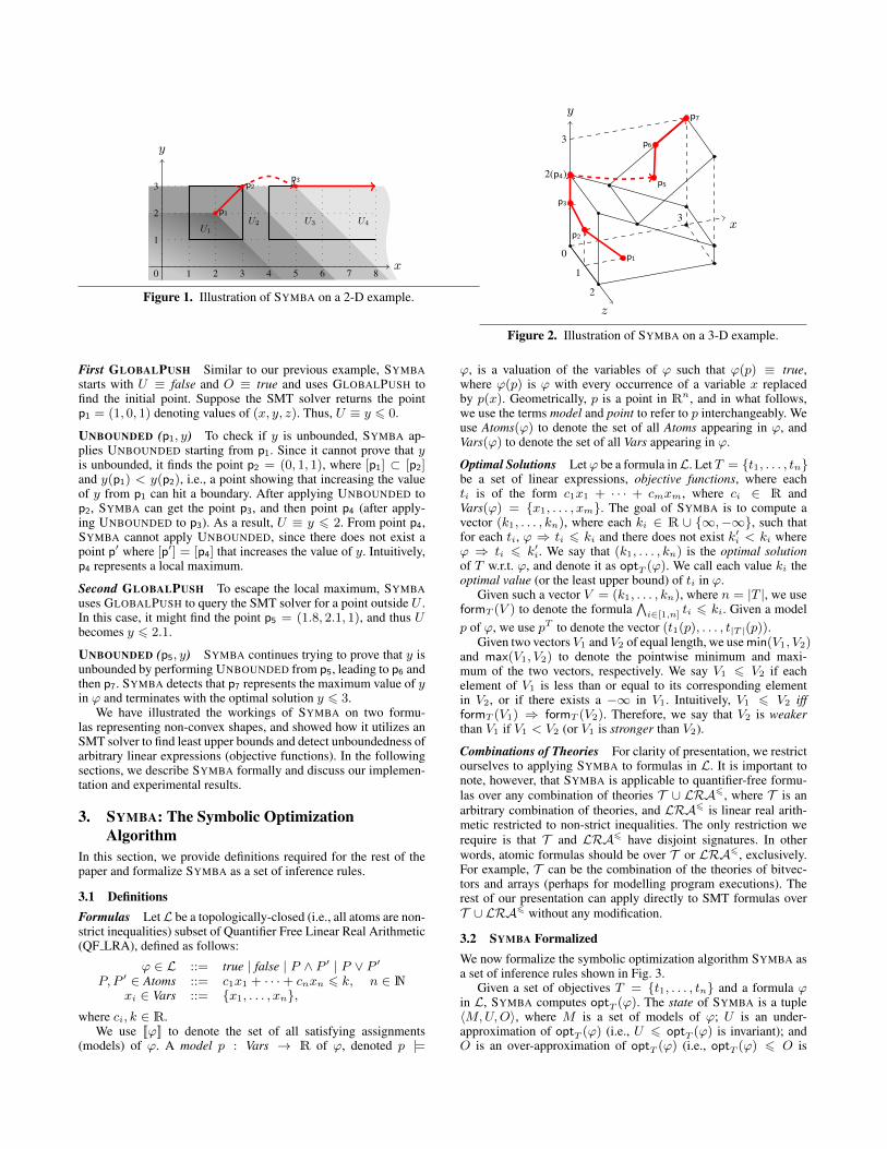
ϕ ≡ 1 6 y 6 3 ∧ (1 6 x 6 3 ∨ x > 4)
containing the real variables x and y and represented pictoriallyby the black boxes in Fig. 1. Suppose that our set of objectives isT = {y, x+y}. That is, we would like to find the least upper boundfor y and x + y in ϕ. (Note that if we want to find the minimumvalue for y, we can simply add −y as an objective to T .) In thisexample, the optimal solution is
optT (ϕ) ≡ y 6 3 ∧ x+ y 6∞,
since x + y is unbounded in ϕ. Formulas of the form t 6 ∞ aretreated as true, and t 6 −∞ as false.
Initially, the under-approximation of optT (ϕ) is
U ≡ y 6 −∞∧ x+ y 6 −∞ ≡ false,
and the over-approximation is
O ≡ y 6∞∧ x+ y 6∞ ≡ true.
SYMBA maintains the invariant U ⇒ optT (ϕ) ⇒ O (note that Uis an under approximation of optT (ϕ), not necessarily ϕ, and sim-ilarly with O). SYMBA alternates between two main operations:GLOBALPUSH, which is used to grow the under-approximation
by sampling points (models) of ϕ that lie outside the under-approximation; and UNBOUNDED, which is used to detect un-bounded objectives. In this example, 3 is the upper bound for y,and x+ y is unbounded.
First GLOBALPUSH SYMBA starts with a GLOBALPUSH byquerying an SMT solver for a model of ϕ that is not a model ofU (i.e., lies outside the under-approximation). Suppose the solverreturns the point p1 = (2, 2). The under-approximation U is thestrongest formula of the form t1 6 k1∧ . . .∧tn 6 kn that containsthe set of points found by the solver (i.e., a convex hull expressedin terms of the objectives). So, the under-approximation is updatedto U ≡ y 6 2 ∧ x + y 6 4 (since the maximum values of y andx + y seen so far are 2 and 4, respectively). This is shown as theshaded region U1 in Fig. 1.
UNBOUNDED (p1, y) SYMBA now tries to prove that y is un-bounded. First, we categorize points into boundary classes as fol-lows: Let E(ϕ) = {l = k | l 6 k ∈ ϕ}, i.e., E(ϕ) is the set ofall atomic formulas appearing in ϕ with the inequalities replacedby equalities. In our example, E(ϕ) = {x = 1, x = 3, x = 4, y =1, y = 3}. Informally, E(ϕ) represents the set of edges (bound-aries) appearing in Fig. 1. The boundary class [p] of a point p is{e ∈ E(ϕ) | p |= e}, i.e., the set of equalities in E(ϕ) satisfied byp. For p1, [p1] = ∅, since p1 does not lie on any of the boundaries.The intuition underlying UNBOUNDED is finding a ray r from apoint p in ϕ such that a given objective t is increasing along r, andr never hits any boundaries of ϕ (i.e., completely contained in ϕ).
UNBOUNDED queries the SMT solver for a point p′ s.t. [p′] =[p1] and y(p1) < y(p′), where y(p′) is the valuation of y atpoint p′. The point p′ = (2, 2.5) satisfies this condition. ThenUNBOUNDED queries for a point p′′ s.t. [p′] ⊂ [p′′] and y(p′) 6y(p′′). If no such p′′ exists, then we know that y is unbounded.Intuitively, we are asking whether we can keep increasing the valueof y from p′ without touching a point p′′ on one of the boundariesin E(ϕ). In this case, such a p′′ exists, so it is added to the under-approximation as p2 = (3, 3) in Fig. 1. Note that p2 exhibits theupper bound of y; SYMBA detects that and strengthens the over-approximation O to y 6 3. After witnessing the point p2, U isupdated to become y 6 3∧x+y 6 6 (see region U2 in the figure).
Second GLOBALPUSH Suppose that SYMBA calls GLOBAL-PUSH. The result is a point in ϕ but not in U . Let p3 = (5, 3)be the point found by GLOBALPUSH. As a result, U is updated toy 6 3 ∧ x+ y 6 8 (see region U3).
UNBOUNDED (p3, x+ y) SYMBA now applies UNBOUNDED tocheck if x+y is unbounded. Suppose UNBOUNDED picks the pointp3. First, it finds a point p′ = (6, 3) which increases x + y and isin the same boundary class as p3. Then, it tries to find a point p′′
that has a boundary class [p′] ⊂ [p′′] and has a greater (or equal)valuation of x + y than p′. Since no such point p′′ exists, SYMBAconcludes that x + y is unbounded. Intuitively, SYMBA discoversthat it is possible to keep finding points along the boundary y = 3that increase x+ y without encountering any other boundary, thusconcluding that x+y is unbounded. We formally specify and provethe correctness of UNBOUNDED in Sec. 3.
The under-approximation U is now updated to become y 6 3(region U4), by dropping the upper bound for x+ y. At this point,U ≡ O, so SYMBA terminates with the optimal solution y 6 3.
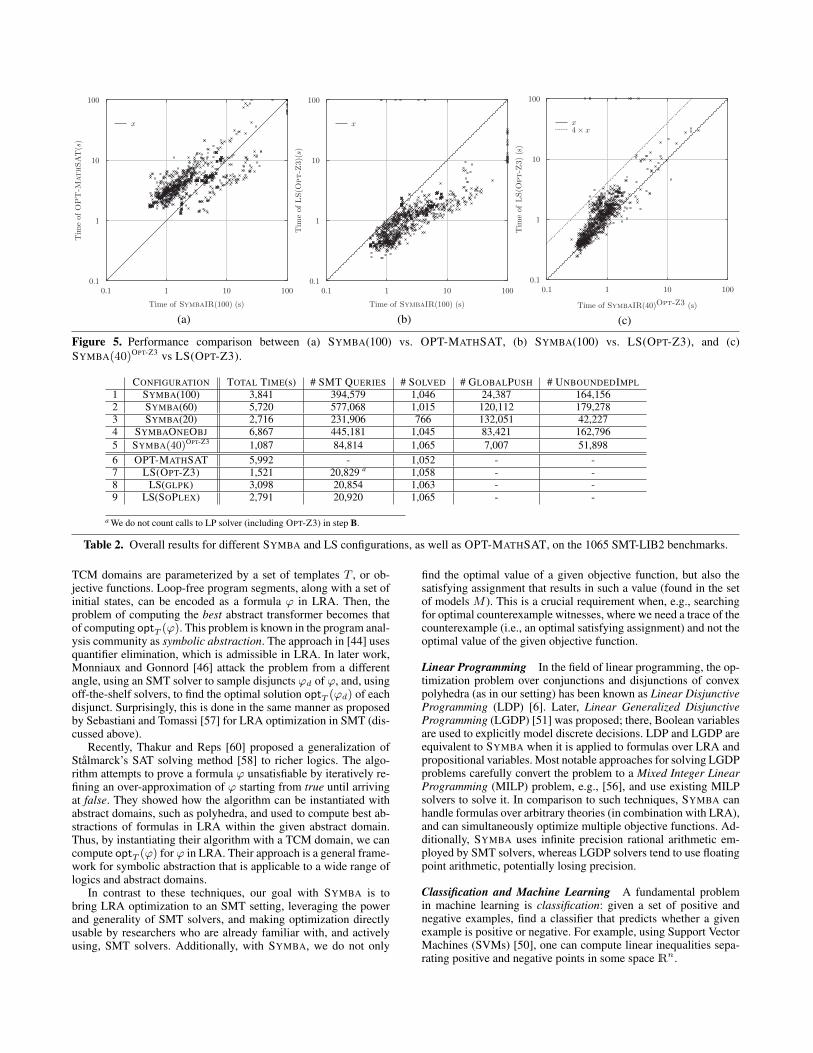
2.2 A 3-dimensional ExampleWe now illustrate the operation of SYMBA on the formula
ϕ ≡ 0 6 x 6 3 ∧ 0 6 z 6 2 ∧ (2y 6 −x+ 4 ∨ 4y = 3x+ 3),
containing the variables x, y, and z and depicted in Fig. 2. Suppose,for simplicity, that we would like to find the least upper bound onlyfor y, i.e., T = {y}.
y
x1 2 3 4 5 6 7 8
1
2
3
p1
p2p3
U1
U2 U3 U4
0
Figure 1. Illustration of SYMBA on a 2-D example.
0
2
3
p7
2(p4)
3
z
x
y
p1
p2
1
p3
p5
p6
Figure 2. Illustration of SYMBA on a 3-D example.
First GLOBALPUSH Similar to our previous example, SYMBAstarts with U ≡ false and O ≡ true and uses GLOBALPUSH tofind the initial point. Suppose the SMT solver returns the pointp1 = (1, 0, 1) denoting values of (x, y, z). Thus, U ≡ y 6 0.
UNBOUNDED (p1, y) To check if y is unbounded, SYMBA ap-plies UNBOUNDED starting from p1. Since it cannot prove that yis unbounded, it finds the point p2 = (0, 1, 1), where [p1] ⊂ [p2]and y(p1) < y(p2), i.e., a point showing that increasing the valueof y from p1 can hit a boundary. After applying UNBOUNDED top2, SYMBA can get the point p3, and then point p4 (after apply-ing UNBOUNDED to p3). As a result, U ≡ y 6 2. From point p4,SYMBA cannot apply UNBOUNDED, since there does not exist apoint p′ where [p′] = [p4] that increases the value of y. Intuitively,p4 represents a local maximum.
Second GLOBALPUSH To escape the local maximum, SYMBAuses GLOBALPUSH to query the SMT solver for a point outside U .In this case, it might find the point p5 = (1.8, 2.1, 1), and thus Ubecomes y 6 2.1.
UNBOUNDED (p5, y) SYMBA continues trying to prove that y isunbounded by performing UNBOUNDED from p5, leading to p6 andthen p7. SYMBA detects that p7 represents the maximum value of yin ϕ and terminates with the optimal solution y 6 3.
We have illustrated the workings of SYMBA on two formu-las representing non-convex shapes, and showed how it utilizes anSMT solver to find least upper bounds and detect unboundedness ofarbitrary linear expressions (objective functions). In the followingsections, we describe SYMBA formally and discuss our implemen-tation and experimental results.
3. SYMBA: The Symbolic OptimizationAlgorithm
In this section, we provide definitions required for the rest of thepaper and formalize SYMBA as a set of inference rules.
3.1 DefinitionsFormulas LetL be a topologically-closed (i.e., all atoms are non-strict inequalities) subset of Quantifier Free Linear Real Arithmetic(QF LRA), defined as follows:
ϕ ∈ L ::= true | false | P ∧ P ′ | P ∨ P ′P, P ′ ∈ Atoms ::= c1x1 + · · ·+ cnxn 6 k, n ∈ N
xi ∈ Vars ::= {x1, . . . , xn},where ci, k ∈ R.
We use JϕK to denote the set of all satisfying assignments(models) of ϕ. A model p : Vars → R of ϕ, denoted p |=
ϕ, is a valuation of the variables of ϕ such that ϕ(p) ≡ true,where ϕ(p) is ϕ with every occurrence of a variable x replacedby p(x). Geometrically, p is a point in Rn, and in what follows,we use the terms model and point to refer to p interchangeably. Weuse Atoms(ϕ) to denote the set of all Atoms appearing in ϕ, andVars(ϕ) to denote the set of all Vars appearing in ϕ.
Optimal Solutions Letϕ be a formula inL. Let T = {t1, . . . , tn}be a set of linear expressions, objective functions, where eachti is of the form c1x1 + · · · + cmxm, where ci ∈ R andVars(ϕ) = {x1, . . . , xm}. The goal of SYMBA is to compute avector (k1, . . . , kn), where each ki ∈ R ∪ {∞,−∞}, such thatfor each ti, ϕ ⇒ ti 6 ki and there does not exist k′i < ki whereϕ ⇒ ti 6 k′i. We say that (k1, . . . , kn) is the optimal solutionof T w.r.t. ϕ, and denote it as optT (ϕ). We call each value ki theoptimal value (or the least upper bound) of ti in ϕ.
Given such a vector V = (k1, . . . , kn), where n = |T |, we useformT (V ) to denote the formula
∧i∈[1,n] ti 6 ki. Given a model
p of ϕ, we use pT to denote the vector (t1(p), . . . , t|T |(p)).Given two vectors V1 and V2 of equal length, we use min(V1, V2)
and max(V1, V2) to denote the pointwise minimum and maxi-mum of the two vectors, respectively. We say V1 6 V2 if eachelement of V1 is less than or equal to its corresponding elementin V2, or if there exists a −∞ in V1. Intuitively, V1 6 V2 iffformT (V1) ⇒ formT (V2). Therefore, we say that V2 is weakerthan V1 if V1 < V2 (or V1 is stronger than V2).
Combinations of Theories For clarity of presentation, we restrictourselves to applying SYMBA to formulas in L. It is important tonote, however, that SYMBA is applicable to quantifier-free formu-las over any combination of theories T ∪ LRA6, where T is anarbitrary combination of theories, and LRA6 is linear real arith-metic restricted to non-strict inequalities. The only restriction werequire is that T and LRA6 have disjoint signatures. In otherwords, atomic formulas should be over T or LRA6, exclusively.For example, T can be the combination of the theories of bitvec-tors and arrays (perhaps for modelling program executions). Therest of our presentation can apply directly to SMT formulas overT ∪ LRA6 without any modification.
3.2 SYMBA FormalizedWe now formalize the symbolic optimization algorithm SYMBA asa set of inference rules shown in Fig. 3.
Given a set of objectives T = {t1, . . . , tn} and a formula ϕin L, SYMBA computes optT (ϕ). The state of SYMBA is a tuple〈M,U,O〉, where M is a set of models of ϕ; U is an under-approximation of optT (ϕ) (i.e., U 6 optT (ϕ) is invariant); andO is an over-approximation of optT (ϕ) (i.e., optT (ϕ) 6 O is

INIT〈∅, (−∞, . . . ,−∞), (∞, . . . ,∞)〉
p |= ϕ ∧ ¬formT (U)GLOBALPUSH
〈M,U,O〉 → 〈M ∪ {p},max(U, pT ), O〉
U = (k1, . . . , kn) p2 |= ϕ [p2] = [p1] ti(p1) < ti(p2)@p3 |= ϕ · ti(p2) 6 ti(p3) ∧ [p2] ⊂ [p3]
UNBOUNDED(p1 ∈M, ti ∈ T )〈M,U,O〉 → 〈M,max(U, (k1, . . . , ki−1,∞, ki+1, . . . , kn)), O〉
p2, p3 |= ϕ ti(p1) < ti(p2) 6 ti(p3) [p1] = [p2] ⊂ [p3]UNBOUNDED-FAIL(p1 ∈M, ti ∈ T )
〈M,U,O〉 → 〈M ∪ {p3},max(U, pT3 ), O〉
O = (k1, . . . , kn) m = max{ti(p′) | p′ ∈M} ϕ⇒ ti 6 mBOUNDED(ti ∈ T )
〈M,U,O〉 → 〈M,U,min(O, (k1, . . . , ki−1,m, ki+1, . . . , kn))〉
Figure 3. Inference rules used by SYMBA.
invariant). Note that for clarity of presentation, we treated optT (ϕ),U , and O as formulas in Sec. 2, whereas here we treat them asvectors and use formT (V ) to convert a vector V to the formula itrepresents.
When SYMBA terminates, we know that U = O = optT (ϕ).Initially, as defined by the rule INIT,M = ∅,U = (−∞, . . . ,−∞),and O = (∞, . . . ,∞). The rules GLOBALPUSH, UNBOUNDED,and UNBOUNDED-FAIL are used to weaken U until it is equal tooptT (ϕ), whereas BOUNDED strengthens O until it is equal tooptT (ϕ).
GLOBALPUSH finds a model of ϕ that is not captured byformT (U) (i.e., lies outside the under-approximation) and addsit to U to weaken it (using max). When the rule GLOBALPUSH nolonger applies, we know thatU = optT (ϕ). Note that applying thisrule alone does not guarantee that U eventually reaches optT (ϕ)for two reasons:
1. Since we are dealing with real variables, GLOBALPUSH mightkeep finding models that approach the upper bound of one ofthe objectives asymptotically.
2. GLOBALPUSH cannot detect whether an objective is unbounded,so it will keep finding models that increase the value of the un-bounded objective indefinitely.
To that end, the rules UNBOUNDED and UNBOUNDED-FAIL areused to detect unbounded objectives and help GLOBALPUSH avoidasymptotic behavior. UNBOUNDED takes as parameters a modelp1 ∈ M and an objective ti ∈ T and attempts to prove that ti isunbounded as follows: First, it tries to find a point p2 |= ϕ such that[p1] = [p2] and t(p1) < t(p2). Then, it looks for a point p3 suchthat p3 |= ϕ, [p2] ⊂ [p3] and t(p2) 6 t(p3). If no such p3 exists,then t is unbounded in ϕ. Otherwise, UNBOUNDED-FAIL adds p3to M . The intuition here is as follows: If we can find a model p2,then we know that t can increase along the hyperplanes in E(ϕ). Ifno point p3 exists, then we know that we can keep increasing t in-definitely without encountering any of the boundaries in E(ϕ) thatare not in [p2], thus showing that t is unbounded. This is analogousto the technique used by the simplex method for showing that a di-mension is unbounded in a convex polyhedron. We further discussthe intuition underlying UNBOUNDED and prove its correctness inSec. 3.3.
In addition to the aforementioned rules, the rule BOUNDED de-tects whether a model p ∈ M exhibits the least upper bound ofsome objective t, and strengthens the over-approximation accord-ingly. Note that the over-approximation is not required for the cor-rectness of SYMBA, but its availability allows us to guarantee that
SYMBA maintains a sound approximation O of optT (ϕ) at everypoint of its execution. This makes SYMBA resilient to SMT solverfailures and allows us to limit resource consumption when desired.That is, by prematurely terminating SYMBA during its execution,we can recover optimal values of some of the objective functions,as maintained by the over-approximation.
Example We illustrate the applications of the rules on the 2-Dexample from Sec. 2.1 and shown in Fig. 1. Assume that after theinitial call to GLOBALPUSH, M = {p1 = (2, 2)}, formT (U) ≡y 6 2 ∧ x+ y 6 4, and formT (O) ≡ true.
Applying UNBOUNDED-FAIL to p1 ∈M and y ∈ T adds p2 =(3, 3) to M . Next, BOUNDED is used to detect that p2 exhibits theleast upper bound of y, and updates O so that formT (O) ≡ y 6 3.
Assume that the second application of GLOBALPUSH addspoint p3 = (5, 3) toM . Applying UNBOUNDED(p3, x+y) detectsthat x+ y is unbounded. At this point, formT (U) becomes y 6 3,making GLOBALPUSH inapplicable. Therefore, ϕ ⇒ formT (U),and U = O = optT (ϕ).
In what follows, we discuss and prove soundness of SYMBA,and define terminating sequences of rule applications.
3.3 SoundnessWe start by showing soundness of the UNBOUNDED rule.
A necessary and sufficient condition for proving that a givenobjective t is unbounded within ϕ is the existence of a convexpolyhedron ϕc, e.g., a ray, such that t is unbounded in ϕc andϕc ⇒ ϕ. Our solution addresses two problems:
1. How to restrict the space from which ϕc is drawn while main-taining completeness, i.e., ensuring that ϕc is found whenever tis unbounded in ϕ.
2. How to check that ϕc ⇒ ϕ.
The idea we use here is to restrict ϕc to formulas of the form∧E ∧ t > k,
where E ⊆ E(ϕ) and k ∈ R. This space of convex polyhedrais sufficient for completeness. For instance, consider the examplefrom Fig. 1. To prove that the x+y direction is unbounded, we finda point p3 = (5, 3) that lies on the boundary y = 3 ∈ E(ϕ) and askwhether ϕc ≡ y = 3 ∧ x+ y > 8 is contained in ϕ. Furthermore,we perform the containment check implicitly by checking whetherthere is a point in ϕc, along any direction that increases x + y,that intersects a boundary of ϕ. In our running example, such apoint does not exist (see Fig. 1). Thus, x + y is unbounded. For

another example, consider the point p1 = (2, 2). Since p1 doesnot lie on any boundary, to check if x + y is unbounded we askwhether ϕc ≡ x+ y > 4 is contained in ϕ (i.e., we check whetherincreasing x + y in ϕc does not encounter boundaries in ϕ). Thisis not the case, and the counterexample is the point p2, shown inFig. 1, that lies on the boundaries x = 3 and y = 3.
Thm. 1 formalizes this construction using boundary classes andstates its correctness for proving that an objective is unbounded inϕ.
Theorem 1 (Soundness of UNBOUNDED). Given a formula ϕ inL and a linear expression t over the variables of ϕ, then @k ∈R · ϕ ⇒ t 6 k (i.e., t is unbounded) if and only if there existp1, p2 |= ϕ such that
1. t(p1) < t(p2)2. [p1] = [p2]3. @p3 |= ϕ · t(p2) 6 t(p3) ∧ [p2] ⊂ [p3]
Proof. Proofs are available in the appendix.
In other words, if the UNBOUNDED rule was applied, thenϕc ≡ [p2]∧ t > t(p2) is contained in ϕ. In the theorem, conditions1 and 2 imply that t is unbounded within ϕc, and condition 3implies that increasing t in ϕc does not encounter any boundariesof ϕ, i.e., [p2] ∧ t > t(p2) is subsumed by ϕ. It follows from thistheorem that UNBOUNDED maintains the invariant U 6 optT (ϕ),since the optimal solution cannot have a least upper bound for t ifit is unbounded (i.e., the least upper bound of t is∞).
Theorem 2 (Soundness of SYMBA). If GLOBALPUSH does notapply, i.e., ϕ ∧ ¬formT (U)⇒ false , then U = optT (ϕ).
Proof. Follows trivially from the invariant U 6 optT (ϕ).
3.4 TerminationWe now discuss sufficient conditions for ensuring termination ofSYMBA. For simplicity of presentation, we assume that T containsa single objective t. We start by defining a fairness condition on thescheduling of SYMBA’s rules that ensures termination.
A fair scheduling is an infinite sequence of actions a1, a2, . . .,where ai ∈ {GLOBALPUSH,UNBOUNDED,UNBOUNDED-FAIL},and the following conditions apply:
1. GLOBALPUSH appears infinitely often, and
2. if a point p is added to M along the execution sequence, thenboth UNBOUNDED(p, t) and UNBOUNDED-FAIL(p, t) eventu-ally appear.
Condition 1 ensures that SYMBA does not get stuck in a lo-cal maximum. Condition 2 ensures that we visit every local max-imum by visiting every boundary class, thus guaranteeing that ei-ther the least upper bound of t is found or it is proved unbounded.Recall the 3-D example from Sec. 2, where T = {y}. Supposeour execution only applies the GLOBALPUSH rule. Then U mightgrow asymptotically towards the least upper bound of y, e.g., y 62, y 6 2.1, y 6 2.11, etc., never reaching y 6 3. Condition 2forces computing models that lie on one or more of the boundariesE(ϕ), thus avoiding this asymptotic behaviour. But applying UN-BOUNDED and UNBOUNDED-FAIL alone without applying GLOB-ALPUSH might get us stuck in local maxima. For example, on pointp4 in Fig. 2, UNBOUNDED(-FAIL) are inapplicable. Condition 1ensures that we eventually find a model outside the current under-approximation (see p5), thus escaping the local maximum.
A k-sequence for an objective t is a sequence of points p1, . . . , pk,where ∀i > 1 · pi |= ϕ ∧ ([pi] ⊂ [pi+1]) ∧ t(pi) 6 t(pi+1), and
UNOUNDED-FAIL(pk, t) fails to apply. For example, in Fig. 2,p1, p2, p3, p4 is a k-sequence.
Since [pi] for a k-sequence strictly grows in size and the largestboundary class has size at most |Atoms(ϕ)|, a k-sequence is oflength at most k = |Atoms(ϕ)|. Lemma 1 states that the last modelpk of a k-sequence always exhibits the largest value of t in itsboundary class [pk].
Lemma 1. Let ϕ be a formula, and t be an objective bounded inϕ. Then, in every execution of SYMBA, the last element pk in everyk-sequence for t satisfies t(pk) = max{t(p) | p |= ϕ ∧ [pk]}.
Proof. According to the definition of a k-sequence, UNBOUNDED-FAIL(pk, t) does not apply. Since t is bounded, premises of UN-BOUNDED do not hold either. Combining premises of the two rules,there does not exist p′k |= ϕ ∧ [pk] such that t(pk) < t(p′k). Thus,t(pk) = max{t(p) | p |= ϕ ∧ [pk]}.
We are now ready to prove termination of any fair execution ofSYMBA. We assume that SYMBA terminates when GLOBALPUSHis no longer applicable, i.e., ϕ⇒ formT (U).
Theorem 3. SYMBA terminates after a finite number of actions inany fair execution.
Proof. We split the proof into two cases as follows:Case 1: t is bounded within ϕ. Suppose SYMBA is non-
terminating. Then, in any fair scheduling, infinitely many GLOB-ALPUSH creates infinitely many k-sequences. Following Lemma 1,there are infinitely many models p in the execution sequence suchthat p |= ϕ and t(p) = max{t(p′) | p′ |= ϕ ∧ [p]}. We denotethe set of such points by P . In any fair execution, GLOBALPUSHmust appear after p is added to M . Therefore, there exists a pointp′ ∈ P such that t(p) < t(p′). As a result, there is a sequence ofpoints p1, p2, . . . in P such t(p1) < t(p2) < t(p3) < · · · . Hence,∀i, j · i 6= j ⇒ [pi] 6= [pj ]. Since the number of boundary classesis finite, SYMBA eventually finds the least upper bound of t andterminates.
Case 2: t is unbounded. Using the same argument as above,SYMBA eventually finds a point in an unbounded boundary class(due to the finite number of boundary classes) such that the threeconditions in Thm. 1 hold. After that, GLOBALPUSH becomesinapplicable.
4. Implementation and Evaluation4.1 ImplementationWe have implemented SYMBA in C++, using the Z3 SMT solver [22]for satisfiability queries. Our implementation accepts a formula ϕand a set of objectives T written in the standard SMT-LIB2 [8]format. It then computes the optimal solution optT (ϕ) and returnsthe result. We have made available the executable and benchmarksonline.
Detecting Unbounded Objectives Our implementation of UN-BOUNDED and UNBOUNDED-FAIL exploits the incremental(PUSH/POP) interface that most SMT solvers supply. Moreover, in-stead of implementing the BOUNDED rule explicitly, we show howto update the over-approximation for free, as a side effect of apply-ing the UNBOUNDED rules.
Fig. 4 shows the procedure UNBOUNDEDIMPL: our implemen-tation of the UNBOUNDED rules. We assume that there is a globalSMT context in which the formula ϕ has been asserted. An activeboundary class c and a objective ti are passed in as parameters.U [ti] andO[ti] refer to the i-th element of the vectors U andO, re-spectively. SAT and UNSAT refer to the current state of the SMTcontext, and GETMODEL() returns a model satisfying the current

1: function UNBOUNDIMPL(c ∈ P(E(ϕ)), ti ∈ T )2: PUSH()3: ASSERT(ti > U [ti])4: if UNSAT then5: O[ti]← U [ti]; POP(); return6: ASSERT(
∧c)
7: if UNSAT then8: POP(); return9: ASSERT(
∨(E(ϕ) \ c)))
10: if SAT then . UNBOUNDED-FAIL11: POP(); return GETMODEL()12: else . UNBOUNDED13: U [ti]←∞14: POP(); return
Figure 4. Implementation of UNBOUNDED(-FAIL).
state of the context if one exists. PUSH() and POP() are used to storeand restore the state of the context, respectively.
We start by incrementally asserting the conditions of UN-BOUNDED implicitly. Given c and ti, we know that there is a pre-viously sampled point p1 |= c such that ti(p1) 6 U [ti]. First,in lines 3-8, we check if there exists a model p2 |= ϕ such thatti(p2) > ti(p1) and [p2] = [p1]. We do this in two stages. We firstcheck if there exists p2 such that ti(p2) > ti(p1). If not, we canupdate the over-approximation O accordingly (line 5). Otherwise,we check if there exists p′2 in the same boundary class as p1 (line 6).If no such p′2 exists, then neither UNBOUNDED nor UNBOUNDED-FAIL applies. Given that p′2 exists, we check for the existence ofp3 in a stronger boundary class (lines 9-13). If p3 exists, we applyUNBOUNDED-FAIL; otherwise, we apply UNBOUNDED.
Scheduling Policy Our implementation is a scheduling of SYMBA’srules (Fig. 3) that satisfies the fairness conditions (in Sec. 3.4).
We start by applying the GLOBALPUSH rule to obtain an initialpoint p. We generate a k-sequence starting at p (for each t ∈ T ) byapplying UNBOUNDED(-FAIL) until either UNBOUNDED is appli-cable (in which case the objective is unbounded) or UNBOUNDED-FAIL is not applicable (in which case we apply GLOBALPUSH toobtain a new initial point and start the process again). It is easy tocheck that this is a fair sequence, and therefore this process alwaysterminates.
To evaluate variations of the scheduling policy described above,we instrumented our implementation with a parameter balance ∈(0, 100] which ensures that UNBOUNDEDIMPL does not take morethan balance% of the total execution time. Specifically, duringexecution, if UNBOUNDEDIMPL has taken more than balance% ofthe elapsed time, SYMBA switches to applying the GLOBALPUSHrule until the time taken by UNBOUNDEDIMPL so far is less thanbalance% of the elapsed time. Intuitively, when balance is 100, thedeterministic schedule described above is in effect.
Optimizations Another effective optimization is to limit E(ϕ)to a “relevant” subset when applying the UNBOUNDED rule. Inour experiments, we noticed that the set E(ϕ) of equality con-straints can be quite large, which burdens the SMT solver. Remov-ing irrelevant equality constraints decreases the size of the SMTqueries. To find the set of “relevant” constraints, we define a re-lation ∝: Atoms(ϕ) × Atoms(ϕ) as follows: P ∝ P ′ if and onlyif
1. Vars(P ) ∩ Vars(P ′) 6= ∅, or
2. ∃P ′′ ∈ Atoms(ϕ) · P ∝ P ′′ ∧ P ′′ ∝ P ′,where Vars(P ) is the set of variables appearing in P .
We then define the boundary class of p w.r.t. t as [p]t = {a ∈E(ϕ) | p |= a ∧ t ∝ a}. Removing constraints that are not ∝-related to t corresponds to carrying out our algorithm on the pro-
STATISTIC AVG. MAX. MIN. STD.# of Variables 882 19,170 40 1,647# of Objectives 56 386 20 15# of Nodes in DAG 7,278 127,987 1,121 10,619
Table 1. Aggregate statistics of our 1,065 benchmarks.
jection of ϕ onto a lower-dimensional space, where the projectionis guaranteed to have the same maximum value for t as ϕ; thuscorrectness is not affected.
4.2 Experimental EvaluationOur experimental evaluation is designed to compare SYMBAagainst other symbolic optimization techniques, and to assess theeffectiveness of our different implementation heuristics.
We conducted two classes of experiments: (1) a comparisonwith existing SMT-based optimization techniques [57]; and (2) anevaluation of the effects of different implementation heuristics,as well as information reuse among multiple objectives, on theefficiency of SYMBA. We describe these in detail below.
Benchmarks As discussed in Sec. 1, one possible applicationof optimization is computing abstract transformers for numericalabstract domains. We have incorporated SYMBA into the UFOprogram analysis and verification framework [5] and used it asan abstract transformer (abstract post operator) for the family ofTemplate Constraint Matrix (TCM) domains [55]. A TCM domainis parameterized by a set of templates T = {t1, . . . , tn}, which arelinear expressions over program variables. Given an abstract stateϕpre describing a set of initial (pre) states and a loop-free programfragment encoded as a formula ϕlf, the best (most precise) abstracttransformer for a TCM domain computes the strongest formula∧ti 6 ki that is implied by ϕpre ∧ ϕlf. Thus, we can use SYMBA
to compute the best abstract transformer by simply computingoptT (ϕpre ∧ ϕlf). Note that the TCM domains subsume a numberof popular domains, including intervals, octagons, octahedra, etc.For instance, by setting T to all live variables and their negation atthe destination program location, then we get an intervals domain,since the result of SYMBA can be interpreted as the minimumand maximum value of each program variable after executing theprogram fragment denoted by ϕlf.
We generated our benchmarks from a set of C programs usedin the 2013 Software Verification Competition (SV-COMP) [1].The programs cover a range of software, from Linux and Windowsdevice drivers to models of SSH and sequentialized concurrentSystemC programs.3 We narrowed the set down to 604 C programsthat were not trivially discharged (proved correct or incorrect) byUFO. We instrumented UFO to record abstract post queries inSMT-LIB2 format, and collected 10K+ queries made by UFO onthese C programs.
Each abstract post query is represented by a formula encoding aset of initial states and a program fragment between two cutpoints(as in large block encoding [12, 33]). For the set of objectives, weused all variables (as well as their negation) that are in scope at thedestination cutpoint (i.e., an intervals domain). From the generatedqueries, we selected the hardest 1,065 benchmarks for evaluation(which took SYMBA more than 0.5s to process). Table 1 showsthe average, maximum, minimum, and standard deviation, of thenumber of variables, objective functions, and nodes in the DAGrepresentation of the formulas in our benchmarks. We conductedall of our experiments on a machine running Linux with an Intel i53.1GHz processor and 4GB of RAM.
3 We drew 2,000+ programs from the following SV-COMP cat-egories: ControlFlowIntegers, SystemC, ProductLines, andDeviceDrivers64.

Comparing with Existing Tools To the best of our knowledge,the work of Sebastiani and Tomasi [57] is the only other SMT tech-nique that addresses the problem of finding optimal assignmentsfor LRA objective functions. At a high level, the technique worksas follows:
A Sample a satisfiable disjunct ϕd from a given formula ϕ usingan SMT solver.
B Sinceϕd is a conjunction of atoms, the linear arithmetic atoms inϕd represent a convex polyhedron. So, use any linear program-ming (LP) solver to find the optimal value of a given objectivefunction within the given disjunct.
C Check, using an SMT solver, whether the result is optimal for allof ϕ. If not, go back to step A and sample a new disjunct. Theprocess is guaranteed to terminate since there are finitely manydisjuncts.
We have acquired a binary of the implementation describedin [57] from the authors. Their tool is called OPT-MATHSAT, asit is built in the MATHSAT SMT solver [18]. There are two issuesthreatening the validity of a direct comparison between SYMBA andOPT-MATHSAT: (1) OPT-MATHSAT accepts a single objectivefunction, meaning that we have to call it multiple times per bench-mark, each time with a different objective. Since we do not haveaccess to its source code, we cannot tell if multiple calls to OPT-MATHSAT incur significant pre-processing overhead. (2) Our im-plementation of SYMBA uses Z3 as its underlying SMT solver,whereas OPT-MATHSAT uses MATHSAT.
In order to avoid these issues and establish a fairer comparison,we have implemented two versions of the linear search (LS) algo-rithm proposed in [57] and implemented in OPT-MATHSAT:
1. LS(OPT-Z3): By accessing the available Z3 source code [3],we modified the linear arithmetic solver of Z3 to allow opti-mization of LRA objectives in the satisfying assignments. ADPLL(T ) [26] solver like Z3 lazily finds propositionally satis-fiable disjuncts (conjunctions of atoms) from a given formulaϕ, and uses a (theory) T -solver to decide the satisfiability ofthe atoms (in our case linear constraints) [24]. We instrumentedZ3’s linear arithmetic solver such that it does not terminate im-mediately after the first satisfying assignment is found, but findsan optimal satisfying assignment for a given objective function.This was implemented using the standard incremental simplexsolving procedure under exact (rational) representation. We callthe modified tool OPT-Z3. LS(OPT-Z3) is an implementationof LS in Z3 that uses OPT-Z3 as its LP solver. This is analo-gous to the implementation described in [57], where a modifiedversion of MATHSAT’s linear arithmetic solver is used as theLP solver.
2. LS(LP) uses an off-the-shelf LP solver as its convex optimiza-tion engine. We have chosen two well-known open source LPlibraries: the GNU Linear Programming Kit (GLPK) [40] andthe Sequential Object-oriented Simplex (SOPLEX) [62] 4.
Both versions of LS use Z3 for sampling disjuncts and checkingoptimality (i.e., steps A and C above), but different LP solversfor finding optimal values (step B). Unlike OPT-MATHSAT, bothLS(OPT-Z3) and LS(LP) accept multiple objective functions, andoptimize them simultaneously. Specifically, in step B, they makemultiple calls to the LP solver to find an optimal value for eachobjective function.
4 We used GLPK v4.51 custom-built. The solver implements the primal two-phase simplex method based on floating point arithmetic. We used SOPLEXv1.7.1, which uses floating point arithmetic.
SYMBA Configurations We use the following SYMBA configu-rations:
1. SYMBA(X): SYMBA with different scheduling policies, whereX specifies the value of balance.
2. SYMBAONEOBJ: Same as SYMBA(100), but optimizes a singleobjective at a time. That is, execution is restarted from scratchfor each objective function.
3. SYMBA(X)OPT-Z3: Same as SYMBA(X), but uses Z3 with themodified linear arithmetic solver OPT-Z3 (we describe this inmore detail below).
Results: SYMBA vs. Other Techniques Fig. 5(a) shows the re-sults of running SYMBA(100) vs. OPT-MATHSAT on the 1,065SMT-LIB2 benchmarks with a timeout of 100 seconds per bench-mark. Each point on the graph represents a benchmark. The axescorrespond to the CPU time (measured in seconds—log scale)taken by SYMBA(100) (x-axis) and OPT-MATHSAT (y-axis). Thepoints above the diagonal represent problems where SYMBA isfaster. Points at the top right corner are cases where both OPT-MATHSAT and SYMBA(100) cannot complete the benchmarkin the allotted 100 seconds5. OPT-MATHSAT has 13 timeoutsvs. 19 timeouts by SYMBA(100). Our results clearly show thatSYMBA(100) outperforms OPT-MATHSAT on our set of bench-marks in most cases. The average and maximum speed up ofSYMBA(100) vs. OPT-MATHSAT are 2.2x and 10.4x, respectively.
We now compare SYMBA against our multi-objective-functionimplementation of the linear search algorithm employed by OPT-MATHSAT. Fig. 5(b) compares the execution times of SYMBA(100)vs. LS(OPT-Z3). The results clearly demonstrate the superior per-formance of LS(OPT-Z3): most benchmarks are solved in less timeby LS(OPT-Z3), often by an order of magnitude. LS(OPT-Z3) has7 timeouts.
To understand the reasons behind these performance differ-ences, we took a closer look at the benchmarks where SYMBA(100)is significantly slower than LS(OPT-Z3). We noticed two recur-ring problems for SYMBA on these benchmarks: (1) the major-ity of the time is spent in the UNBOUNDEDIMPL function, indi-cating the expensive nature of UNBOUNDEDIMPL calls and inef-fectiveness of our scheduling strategy when balance=100; (2) ap-plications of GLOBALPUSH make very small expansions to theunder-approximation U , indicating that we prefer guided applica-tions of GLOBALPUSH. To address point (1), we ensured that UN-BOUNDEDIMPL does not take more than 40% of the execution timeby setting balance to 40. To address point (2), we considered ap-plying GLOBALPUSH using OPT-Z3 (described above) instead ofZ3. That is, instead of GLOBALPUSH asking Z3 for a point that liesoutside the under-approximation U , we made GLOBALPUSH sup-ply OPT-Z3 with one of the objective functions, and whenever theZ3’s DPLL(T ) solver finds a satisfiable disjunct with a point out-side the under-approximation, it finds a satisfying assignment thatmaximizes that objective function within that disjunct. This causesthe GLOBALPUSH rule to produce models that are farther awayfrom the current under-approximation, expediting convergence. Wecall this configuration SYMBA(40)OPT-Z3.
Fig. 5(c) compares the execution times of SYMBA(40)OPT-Z3 vs.LS(OPT-Z3). The results now show that SYMBA(40)OPT-Z3 out-performs LS(OPT-Z3) on 81% of the benchmarks, with a 5.0xmaximum speedup and a 1.4x average speedup per benchmark.Moreover, SYMBA(40)OPT-Z3 solves all 1,065 benchmarks withouttiming out. We have also run the two other configurations of lin-
5 Since OPT-MATHSAT accepts a single objective at a time, we invokedit multiple times per benchmark, giving it a timeout of 100 seconds perobjective. If the total time (for all objectives) taken for a benchmark is morethan 100 seconds, OPT-MATHSAT is considered to have timed out.

ear search, LS(GLPK) and LS(SOPLEX). They exhibit similar be-haviour to LS(OPT-Z3), but are slightly slower. We cross-checkedall results produced by different tools (when they do not timeout)and all of them match.
Results: SYMBA’s Configurations Table 2 summarizes the re-sults of running all the aforementioned algorithms and configura-tions on the same set of benchmarks with a timeout of 100 secondsper benchmark. The results of running SYMBA(100) are summa-rized in row 1 of Table 2. SYMBA(100) was able to solve 1,046out of 1,065 benchmarks in 3,841 seconds. In the process, it made∼395K SMT queries using 24,387 invocations of GLOBALPUSHand 164,156 invocations of UNBOUNDEDIMPL.
Rows 2-3 capture the results of running SYMBA(X), whereX is 60 and 20, respectively. When X is 60 (time spent in UN-BOUNDEDIMPL is restricted to 60% of the total time) the num-ber of GLOBALPUSH calls goes up by about 400%. Time is spentin making unguided discovery rather than big leap towards thegoal. This even affects UNBOUNDEDIMPL, the number of callsslightly increases since more points are sampled. When X is 20,it was only able to solve 766 benchmarks, for which the numberof calls to GLOBALPUSH goes above 130K while the number ofcalls to UNBOUNDEDIMPL drops to ∼42K. Our experiments showthat 100 is the best value for balance when running SYMBA(X)6.Conversely, when running SYMBA(X)OPT-Z3, we found that wegreatly benefit from a lower balance value (balance=40 gives usbest performance), since there the GLOBALPUSH rule can discoverunbounded objectives, alleviating the pressure on UNBOUNDED-IMPL.
SYMBAONEOBJ (see Row 4 of Table 2) was able to solve 1,045problems in 6,867 seconds. SYMBAONEOBJ uses the same config-uration as SYMBA(100) except that it finds solutions for multipleobjectives independently, without reusing models amongst differ-ent objectives (as SYMBA does). Using SYMBAONEOBJ causesthe number of SMT queries to go up by 15% and the number ofGLOBALPUSH calls to increase by 300%. Optimizing multiple ob-jective functions simultaneously ensures that all objectives benefitfrom the sampled models and potentially avoids repeating expen-sive SMT calls.
Summary The experiments compare our proposed SMT-basedsymbolic optimization algorithm with existing techniques andhighlight the effectiveness of various implementation heuristicsand optimizations. We compared SYMBA with OPT-MATHSATas well as two LP based implementations of its algorithm on alarge set of benchmarks generated from program analysis tasks.The results demonstrate the power of SYMBA’s approach. A con-figuration that employs both efficient scheduling policy and convexoptimization outperforms them all and solves all the benchmarks.Our experiments also demonstrate the importance of SYMBA’smulti-objective-function capability.
5. Related WorkOur work intersects with different areas of research. In this section,we compare SYMBA with (1) other optimization techniques in SATand SMT solvers; (2) optimization techniques employed within thecontext of abstract interpretation [21]; (3) linear programming tech-niques; and (4) classification techniques from the machine learningcommunity.
Optimization in SAT/SMT Within the SMT and SAT solvingarena, numerous forms of optimization have been proposed (e.g.,MAX-SAT/SMT in Yices [2]). The closest to SYMBA is the re-cent of work of Sebastiani and Tomasi [57]. Similar to SYMBA,
6 We omit SYMBA(40) and SYMBA(80) from the table as they exhibitsimilar performance to SYMBA(60).
they propose an SMT-based solution for optimizing objective func-tions in LRA, and to the best of our knowledge, this is the onlyother work that addresses this problem. As explained in Sec. 4, thisapproach works by sampling a satisfiable disjunct (convex polyhe-dron) from a given formula using the SMT solver as a black box.Then, using any LP solver, it finds the optimal value of an objec-tive function in that disjunct. It then checks if the optimal value isglobally optimal (again, using the SMT solver); otherwise, moredisjuncts are sampled. Effectively, this approach lazily builds theDNF of a formula until the disjunct with the optimal value of agiven objective function is found. Compared to [57], SYMBA doesnot require an off-the-shelf LP solver (or access to a modified the-ory solver within the SMT solver [57]) Instead, SYMBA offers asimple and elegant optimization algorithm that can be easily imple-mented on top of existing SMT solvers, without using any externaltools. Moreover, SYMBA can simultaneously optimize multiple ob-jective functions. SYMBA also maintains an over-approximation ofthe optimal solution, allowing us to prematurely terminate it andstill retrieve optimal values for a subset of the objective functions.As we show in Sec. 4, the multi-objective-function feature can alsobe implemented within the approach of [57]. Both SYMBA and [57]can apply to formulas over mixed theories.
In [17], Cimatti et al. proposed a theory of costs for augmentingan SMT solver with pseudo-boolean (PB) constraints [11]. At ahigh level, their theory allows associating a cost with individualBoolean constraints. The goal then is to find a satisfying assignmentthat minimizes/maximizes the total cost. Thus, the theory of costsenables encoding weighted MAX-SAT/SMT problems – in fact, thetwo problems are equivalent. It is easy to see that SYMBA subsumesthe weighted MAX-SMT problem. For example, we can associatewith each Boolean constraint Bi a cost ci, and add a constraintite(Bi, ci = ki, ci = 0), where ki ∈ R. Then, our objective is tominimize or maximize the sum of all costs c1 + . . .+ cn.
Another form of optimization in the SMT framework is that ofNieuwenhuis and Oliveras [47]. Their optimization technique ex-tends the traditional DPLL(T ) algorithm for SMT solving with ex-tra rules for strengthening the theory T midway during execution,e.g., a theory solver for linear arithmetic might be strengthened tofind only assignments with values less than 10. This allows guidingthe solver towards satisfying assignments that maximize or mini-mize certain objective functions. The authors show how to imple-ment weighted MAX-SMT in their general framework. It is unclearto us if their theory strengthening approach can be used to imple-ment an optimization procedure for LRA objective functions (as inthis paper). Moreover, unlike SYMBA, their approach is not easilyimplementable, as it requires deep modifications to an SMT solver.
In more recent work [16], Chaganty et al. consider the problemof finding most likely satisfying assignments in the presence ofprobabilistic constraints. There, an SMT solver is used to handleaxioms, i.e., constraints with 0 or 1 probabilities, and a relationalsolver (e.g., [48]) is used to handle other probabilistic constraints.It is important to note that the relational solver can be replacedby a weighted MAX-SMT solver (as noted in [16]). Thus, SYMBAcan be directly applicable to solving such problems. We leave thisinteresting direction for future work.
Optimization in Abstract Interpretation Numerical abstract do-mains have been an active subject of research due to their impor-tance in different program analyses. As discussed earlier, an impor-tant operation in such domains is the abstract transformer (post),which can often be phrased as an optimization problem over formu-las in LRA. As a result, optimization has been a subject of interestwithin the program analysis community.
For example, Monniaux [44] proposed an algorithm for com-puting best abstract transformers of Template Constraint Matrix(TCM) domains [55] over loop-free code. As discussed in Sec. 4,
0.1 1 10 100
Time of SymbaIR(100) (s)
0.1
1
10
100
Tim
eof
OPT-M
athSAT(s)
x
(a)
0.1 1 10 100
Time of SymbaIR(100) (s)
0.1
1
10
100
Tim
eof
LS(O
pt-Z
3)(s)
x
(b)
0.1 1 10 100
Time of SymbaIR(40)Opt-Z3 (s)
0.1
1
10
100
Tim
eof
LS(O
pt-Z
3)(s)
x4× x
(c)
Figure 5. Performance comparison between (a) SYMBA(100) vs. OPT-MATHSAT, (b) SYMBA(100) vs. LS(OPT-Z3), and (c)SYMBA(40)OPT-Z3 vs LS(OPT-Z3).
CONFIGURATION TOTAL TIME(s) # SMT QUERIES # SOLVED # GLOBALPUSH # UNBOUNDEDIMPL1 SYMBA(100) 3,841 394,579 1,046 24,387 164,1562 SYMBA(60) 5,720 577,068 1,015 120,112 179,2783 SYMBA(20) 2,716 231,906 766 132,051 42,2274 SYMBAONEOBJ 6,867 445,181 1,045 83,421 162,7965 SYMBA(40)OPT-Z3 1,087 84,814 1,065 7,007 51,8986 OPT-MATHSAT 5,992 - 1,052 - -7 LS(OPT-Z3) 1,521 20,829 a 1,058 - -8 LS(GLPK) 3,098 20,854 1,063 - -9 LS(SOPLEX) 2,791 20,920 1,065 - -
a We do not count calls to LP solver (including OPT-Z3) in step B.
Table 2. Overall results for different SYMBA and LS configurations, as well as OPT-MATHSAT, on the 1065 SMT-LIB2 benchmarks.
TCM domains are parameterized by a set of templates T , or ob-jective functions. Loop-free program segments, along with a set ofinitial states, can be encoded as a formula ϕ in LRA. Then, theproblem of computing the best abstract transformer becomes thatof computing optT (ϕ). This problem is known in the program anal-ysis community as symbolic abstraction. The approach in [44] usesquantifier elimination, which is admissible in LRA. In later work,Monniaux and Gonnord [46] attack the problem from a differentangle, using an SMT solver to sample disjuncts ϕd of ϕ, and, usingoff-the-shelf solvers, to find the optimal solution optT (ϕd) of eachdisjunct. Surprisingly, this is done in the same manner as proposedby Sebastiani and Tomassi [57] for LRA optimization in SMT (dis-cussed above).
Recently, Thakur and Reps [60] proposed a generalization ofStalmarck’s SAT solving method [58] to richer logics. The algo-rithm attempts to prove a formula ϕ unsatisfiable by iteratively re-fining an over-approximation of ϕ starting from true until arrivingat false. They showed how the algorithm can be instantiated withabstract domains, such as polyhedra, and used to compute best ab-stractions of formulas in LRA within the given abstract domain.Thus, by instantiating their algorithm with a TCM domain, we cancompute optT (ϕ) for ϕ in LRA. Their approach is a general frame-work for symbolic abstraction that is applicable to a wide range oflogics and abstract domains.
In contrast to these techniques, our goal with SYMBA is tobring LRA optimization to an SMT setting, leveraging the powerand generality of SMT solvers, and making optimization directlyusable by researchers who are already familiar with, and activelyusing, SMT solvers. Additionally, with SYMBA, we do not only
find the optimal value of a given objective function, but also thesatisfying assignment that results in such a value (found in the setof models M ). This is a crucial requirement when, e.g., searchingfor optimal counterexample witnesses, where we need a trace of thecounterexample (i.e., an optimal satisfying assignment) and not theoptimal value of the given objective function.
Linear Programming In the field of linear programming, the op-timization problem over conjunctions and disjunctions of convexpolyhedra (as in our setting) has been known as Linear DisjunctiveProgramming (LDP) [6]. Later, Linear Generalized DisjunctiveProgramming (LGDP) [51] was proposed; there, Boolean variablesare used to explicitly model discrete decisions. LDP and LGDP areequivalent to SYMBA when it is applied to formulas over LRA andpropositional variables. Most notable approaches for solving LGDPproblems carefully convert the problem to a Mixed Integer LinearProgramming (MILP) problem, e.g., [56], and use existing MILPsolvers to solve it. In comparison to such techniques, SYMBA canhandle formulas over arbitrary theories (in combination with LRA),and can simultaneously optimize multiple objective functions. Ad-ditionally, SYMBA uses infinite precision rational arithmetic em-ployed by SMT solvers, whereas LGDP solvers tend to use floatingpoint arithmetic, potentially losing precision.
Classification and Machine Learning A fundamental problemin machine learning is classification: given a set of positive andnegative examples, find a classifier that predicts whether a givenexample is positive or negative. For example, using Support VectorMachines (SVMs) [50], one can compute linear inequalities sepa-rating positive and negative points in some spaceRn.

SYMBA can be viewed as a sophisticated classification algo-rithm, where positive and negative examples are models of ϕ and¬ϕ, respectively. The goal is to find the best classifier, representedby a conjunction of linear inequalities (objective functions), thatdoes not misclassify any of the positive examples (i.e., is impliedby ϕ). SYMBA only samples positive examples (from ϕ) and keepsweakening a classifier (the under-approximation U ) until it encom-passes all positive examples. As Reps et al. point out in [52], weak-ening an under-approximation by sampling more points is analo-gous to the approach of the simple learning algorithm Find-S [43].Find-S gradually weakens a classifier, starting from false, by itera-tively taking into account more and more positive examples.
6. Conclusions and Future WorkWe proposed SYMBA, an efficient SMT-based optimization algo-rithm for objective functions stated in the theory of linear real arith-metic. SYMBA utilizes efficient SMT solvers as black boxes, mak-ing it easy to implement without requiring modifications to existingintricate SMT solver implementations, and enabling it to directlybenefit from future advances in SMT solving. We have evaluatedSYMBA on benchmarks drawn from abstract transformer compu-tations for numerical abstract domains. Our thorough experimentalevaluation indicates the advantages of our approach over other pro-posed techniques.
We see many avenues for future work. First, the most naturalnext step is extending SYMBA to integer arithmetic objective func-tions. We believe this can be done by augmenting SYMBA’s ruleswith new ones that introduce Gomory cuts (cutting planes) [29] inorder to prune infeasible solutions. Another interesting direction ishandling non-linear objective functions, in order to model complexcost functions. From an engineering perspective, we would also liketo study efficient parallel implementations of SYMBA’s rules.
References[1] Competition On Software Verification - (SV-COMP). http://
sv-comp.sosy-lab.org.[2] Yices SMT Solver. http://yices.csl.sri.com.[3] Z3 Source Code Repository. http://z3.codeplex.com/.[4] A. Albarghouthi and K. L. McMillan. Beautiful Interpolants. In Proc.
of CAV’13, pages 313–329, 2013.[5] A. Albarghouthi, A. Gurfinkel, and M. Chechik. UFO: A Framework
for Abstraction- and Interpolation-Based Software Verification. InProc. of CAV’12, pages 672–678, 2012.
[6] E. Balas. Disjunctive programming: Properties of the convex hull offeasible points. Discrete Applied Mathematics, 89(1–3):3 – 44, 1998.
[7] T. Ball and S. Rajamani. The SLAM Toolkit. In Proc. of CAV’01,volume 2102 of LNCS, pages 260–264, 2001.
[8] C. Barrett, A. Stump, and C. Tinelli. The SMT-LIB Standard: Version2.0. Technical report, Department of Computer Science, The Univer-sity of Iowa, 2010. Available at www.SMT-LIB.org.
[9] C. Barrett, C. Conway, M. Deters, L. Hadarean, D. Jovanovic, T. King,A. Reynolds, and C. Tinelli. CVC4. In Proc. of CAV’11, pages 171–177, 2011.
[10] C. W. Barrett, R. Sebastiani, S. A. Seshia, and C. Tinelli. Satisfiabilitymodulo theories. In Handbook of Satisfiability, pages 825–885. 2009.
[11] P. Barth. A Davis-Putnam based enumeration algorithm for lin-ear pseudo-Boolean optimization. Technical Report MPI-I-95-2-003,Max-Planck-Institute fur Informatik, 1995.
[12] D. Beyer, A. Cimatti, A. Griggio, M. E. Keremoglu, and R. Sebastiani.Software Model Checking via Large-Block Encoding. In Proc. ofFMCAD’09, pages 25–32, 2009.
[13] G. M. Bierman, A. D. Gordon, C. Hritcu, and D. E. Langworthy.Semantic Subtyping with an SMT Solver. J. Funct. Program., 22(1):31–105, 2012.
[14] N. Bjorner, K. McMillan, and A. Rybalchenko. Program Verificationas Satisfiability Modulo Theories. In Proc. of SMT’12, 2012.
[15] C. Cadar, D. Dunbar, and D. R. Engler. KLEE: Unassisted andAutomatic Generation of High-Coverage Tests for Complex SystemsPrograms. In Proc. of OSDI’08, pages 209–224, 2008.
[16] A. Chaganty, A. Lal, A. Nori, and S. Rajamani. Combining RelationalLearning with SMT Solvers using CEGAR. In Proc. of CAV’13, pages447–462, 2013.
[17] A. Cimatti, A. Franzen, A. Griggio, R. Sebastiani, and C. Stenico. Sat-isfiability Modulo the Theory of Costs: Foundations and Applications.In Proc. of TACAS‘10, pages 99–113, 2010.
[18] A. Cimatti, A. Griggio, B. J. Schaafsma, and R. Sebastiani. TheMathSAT5 SMT Solver. In Proc. of TACAS’13, pages 93–107, 2013.
[19] E. Clarke, D. Kroening, and F. Lerda. A Tool for Checking ANSI-CPrograms. In Proc. of TACAS’04, volume 2988 of LNCS, pages 168–176, March 2004.
[20] P. Cousot and R. Cousot. Static Determination of Dynamic Propertiesof Programs. In Proc. of the Colloque sur la Programmation, 1976.
[21] P. Cousot and R. Cousot. Abstract Interpretation: A Unified LatticeModel For Static Analysis of Programs by Construction or Approxi-mation of Fixpoints. In Proc. of POPL’77, pages 238–252, 1977.
[22] L. de Moura and N. Bjørner. Z3: An Efficient SMT Solver. In Proc.of TACAS’08, LNCS, pages 337–340, 2008.
[23] R. DeLine and K. R. M. Leino. BoogiePL: A Typed ProceduralLanguage for Checking Object-oriented Programs. Technical report,Microsoft Research, 2005.
[24] B. Dutertre and L. de Moura. A Fast Linear-Arithmetic Solver forDPLL(T). In Proc. of CAV’06, pages 81–94, 2006.
[25] S. Falke, F. Merz, and C. Sinz. LLBMC: Improved Bounded ModelChecking of C Programs Using LLVM. In Proc. of TACAS’13, pages623–626, 2013.
[26] H. Ganzinger, G. Hagen, R. Nieuwenhuis, A. Oliveras, and C. Tinelli.DPLL(T): Fast Decision Procedures. In Proc. of CAV’04, LNCS,pages 175–188, 2004.
[27] P. Godefroid, N. Klarlund, and K. Sen. DART: Directed AutomatedRandom Testing. In Proc. of PLDI’05, pages 213–223, 2005.
[28] P. Godefroid, M. Y. Levin, and D. A. Molnar. SAGE: WhiteboxFuzzing for Security Testing. Commun. ACM, 55(3):40–44, 2012.
[29] R. E. Gomory. Outline of an Algorithm for Integer Solutions to LinearPrograms. Bull. Amer. Math. Soc., 64(5):275–278, 1958.
[30] S. Grebenshchikov, N. P. Lopes, C. Popeea, and A. Rybalchenko. Syn-thesizing Software Verifiers from Proof Rules. In Proc. of PLDI’12,pages 405–416, 2012.
[31] S. Gulwani, S. Jha, A. Tiwari, and R. Venkatesan. Synthesis of Loop-Free Programs. In Proc. of PLDI’11, pages 62–73, 2011.
[32] A. Gupta, C. Popeea, and A. Rybalchenko. Solving Recursion-FreeHorn Clauses over LI+UIF. In Proc. of APLAS’11, pages 188–203,2011.
[33] A. Gurfinkel, S. Chaki, and S. Sapra. Efficient Predicate Abstractionof Program Summaries. In Proc. of NFM’11, volume 6617 of LNCS,pages 131–145, 2011.
[34] W. R. Harris, S. Sankaranarayanan, F. Ivancic, and A. Gupta. Pro-gram Analysis via Satisfiability Modulo Path Programs. In Proc. ofPOPL’10, pages 71–82, 2010.
[35] T. Henzinger, R. Jhala, R. Majumdar, and G. Sutre. Lazy Abstraction.In Proc. of POPL’02, pages 58–70, 2002.
[36] T. A. Henzinger, R. Jhala, R. Majumdar, and K. L. McMillan. Ab-stractions from Proofs. In Proc. of POPL’04, pages 232–244, 2004.
[37] S. Jha, S. Gulwani, S. A. Seshia, and A. Tiwari. Oracle-GuidedComponent-Based Program Synthesis. In Proc. of ICSE’10, pages215–224, 2010.
[38] A. S. Koksal, V. Kuncak, and P. Suter. Constraints as Control. In Proc.of POPL’12, pages 151–164, 2012.
[39] K. R. M. Leino. Dafny: An Automatic Program Verifier for FunctionalCorrectness. In Proc. of LPAR’10, pages 348–370, 2010.

[40] A. Makhorin. The GNU Linear Programming Kit.http://www.gnu.org/software/glpk/, 2000.
[41] H. Massalin. Superoptimizer: a Look at the Smallest Program.SIGARCH Comput. Archit. News, 15(5):122–126, Oct. 1987.
[42] A. Mine. The Octagon Abstract Domain. J. Higher-Order andSymbolic Computation, 19(1):31–100, 2006.
[43] T. M. Mitchell. Machine Learning. McGraw-Hill, Inc., New York,NY, USA, 1997.
[44] D. Monniaux. Automatic Modular Abstractions for Linear Con-straints. In Proc. of POPL’09, pages 140–151, 2009.
[45] D. Monniaux. Automatic Modular Abstractions for Template Numer-ical Constraints. Logical Methods in Computer Science, 6(3), 2010.
[46] D. Monniaux and L. Gonnord. Using Bounded Model Checking toFocus Fixpoint Iterations. In Proc. of SAS’11, pages 369–385, 2011.
[47] R. Nieuwenhuis and A. Oliveras. On SAT Modulo Theories andOptimization Problems. In Proc. of SAT’06, pages 156–169, 2006.
[48] F. Niu, C. Re, A. Doan, and J. Shavlik. Tuffy: Scaling Up StatisticalInference in Markov Logic Networks Using an RDBMS. Proc. ofVLDB’11, pages 373–384, 2011.
[49] R. Piskac, T. Wies, and D. Zufferey. Automating Separation Logicusing SMT. In Proc. of CAV’13, 2013.
[50] J. C. Platt. Fast Training of Support Vector Machines Using SequentialMinimal Optimization. In Advances in Kernel Methods, pages 185–208. MIT Press, 1999.
[51] R. Raman and I. Grossmann. Modelling and Computational Tech-niques for Logic Based Integer Programming. Computers and Chem-ical Engineering, 18(7):563 – 578, 1994.
[52] T. Reps, M. Sagiv, and G. Yorsh. Symbolic Implementation of the BestTransformer. In Proc. of VMCAI’04, volume 2937 of LNCS, 2004.
[53] P. M. Rondon, M. Kawaguchi, and R. Jhala. Liquid Types. In Proc. ofPLDI’08, pages 159–169, 2008.
[54] A. Rybalchenko and V. Sofronie-Stokkermans. Constraint Solving forInterpolation. J. Symb. Comput., 45(11):1212–1233, 2010.
[55] S. Sankaranarayanan, H. B. Sipma, and Z. Manna. Scalable Analysisof Linear Systems using Mathematical Programming. In Proc. ofVMCAI’05, pages 25–41, 2005.
[56] N. W. Sawaya and I. E. Grossmann. A Cutting Plane Method for Solv-ing Linear Generalized Disjunctive Programming Problems. Comput-ers And Chemical Engineering, 29(9):1891 – 1913, 2005.
[57] R. Sebastiani and S. Tomasi. Optimization in SMT with LA(Q) CostFunctions. In Proc. of IJCAR‘12, pages 484–498, 2012.
[58] M. Sheeran and G. Stamarck. A Tutorial on Stalmarck’s Proof Proce-dure for Propositional Logic. FMSD, 16:23–58, 2000.
[59] A. Solar-Lezama, L. Tancau, R. Bodık, S. A. Seshia, and V. A.Saraswat. Combinatorial Sketching for Finite Programs. In Proc. ofASPLOS’06, pages 404–415, 2006.
[60] A. V. Thakur and T. W. Reps. A Method for Symbolic Computationof Abstract Operations. In Proc. of CAV’12, pages 174–192, 2012.
[61] A. V. Thakur, M. Elder, and T. W. Reps. Bilateral Algorithms forSymbolic Abstraction. In Proc. of SAS’12, pages 111–128, 2012.
[62] R. Wunderling. Paralleler und Objekt-orientierter Simplex-Algorithmus. PhD thesis, Technische Universitat Berlin, 1996.
7. AppendixLemma 2. Given an L formula ϕc defining a convex polyhedron(conjunction of linear constraints), if p |= ϕc, [p] ⊆ [p′], t(p) 6t(p′) and @p′′ |= ϕc · t(p) 6 t(p′′) ∧ [p] ⊂ [p′′], then p′ |= ϕc.
Proof. Formula ϕc ∧ [p] can be written as a system of linear in-equalities as follows:
A~x = ~b (1a)
C~x > ~d (1b)
By definition, p satisfies the system and Eq. 1a is a subset of [p]according to the definition of boundary class. Because [p] ⊆ [p′],p′ must satisfy Eq. 1a. Suppose p′ 2 ϕc. Then there exists some ksuch that ~ck · ~p > dk and ~ck · ~p′ < dk
Note that ~ck · ~p 6= dk since ~ck · ~p′ 6= dk and [p] ⊆ [p′]. We nowshow that there exists a point ~pk = α~p+(1−α)~p′ (0 < α < 1) inthe convex hull of p and p′ s.t. ~ck · ~pk = dk. Since t(p) 6 t(p′), it iseasy to show that t(p) 6 t(pk). Let ~ck·~p = dk+δ1, ~ck·~p′ = dk−δ2(where δ1 > 0 and δ2 > 0), and α = δ2
δ1+δ2. We have ~ck · ~pk = dk.
We know that [p] ⊂ [pk] because pk is in the convex hull of p andp′ and {~ck · ~x = dk} /∈ [p] ∧ {~ck · ~x = dk} ∈ [pk].
Suppose pk 2 ϕc, i.e., there exists j s.t. ~cj · ~pk < dj , wethen repeat the above process. Each point pi found satisfies t(p) 6t(pi) ∧ [p] ⊂ [pi]. We are guaranteed to find a point p′′ in theconvex hull s.t. it is also within ϕc, because in each step wesatisfy at least one more inequality. This contradicts the condition@p′′ |= ϕc · t(p) 6 t(p′′) ∧ [p] ⊂ [p′′]. Therefore, p′ |= ϕc.
Proof of Thm. 1 (⇐) We prove this direction by contradiction.First, let p1, p2 |= ϕ be two models satisfying the three conditionsof the theorem. Suppose there is a point p∗ |= ϕ s.t. t(p∗) is theupper bound for t inϕ. We show that there is always a point p′2 |= ϕs.t. t(p′2) > t(p∗).
Pick a point p′2 s.t. ~p′2 = ~p2 + λ( ~p2 − ~p1). It follows thatt(p′2) > t(p∗) when λ > ( ~p∗− ~p2)·~t
( ~p2− ~p1)·~t. The notation ~p denotes the
vector representation (p(x1), . . . , p(xn)) of the model p : Vars→R, where Vars = {x1, . . . , xn}.
Let the formula ϕ′ define a convex polyhedron s.t. p2 |= ϕ′ andϕ′ ⇒ ϕ. Let ϕc ≡ ϕ′ ∧
∧[p2]. We know the following:
1. ϕc defines a convex polyhedron (by its definition).
2. @p′′2 |= ϕc · t(p2) 6 t(p′′2 ) ∧ [p2] ⊂ [p′′2 ] (by condition 3 of thetheorem).
3. [p2] ⊆ [p′2] (since p′2 is in the affine set of p1 and p2).
4. t(p2) 6 t(p′2) (since λ > 0).
Following the result of Lemma 2, p′2 is in ϕc which is also in ϕ.This contradicts the assumption that t(p∗) is the least upper boundfor t. Therefore, term t is unbounded in ϕ.
(⇒) Given that t is unbounded in ϕ, we look for two modelsp1, p2 |= ϕ that satisfy the required conditions. Pick p1, p2 |= ϕs.t. [p1] = [p2], t(p2) > t(p1), and [p1] is the most restrictiveboundary class within which t is unbounded (i.e., t is unbounded inϕ∧
∧[p1], and there does not exist a boundary class c ⊃ [p1] s.t. t is
unbounded in ϕ∧∧c). We know that such a class exists because t
is unbounded in ϕ (otherwise t is bounded in every boundary classand ϕ is bounded). In other words, since (1) there are infinitelymany models of ϕ with increasing values of t and (2) finitely manyboundary classes, there has to be a boundary class [p1] s.t. t isunbounded in ϕ ∧
∧[p1] and there doesn’t exist a class c ⊃ [p1]
where t is unbounded in ϕ ∧∧c.
If there are no classes c ⊃ [p1], or for every c ⊃ [p1], ϕ∧∧c⇒
false, then p1 and p2 satisfy the three conditions of the theorem.Otherwise, let m = maxp|=ϕ∧ψt(p), where ψ ≡
∨c⊃[p1]
∧c (i.e.,
all classes stronger than [p1]). We know that m is defined (i.e., not∞) because of our assumption on the class [p1]. Ifm < t(p2), thenp1 and p2 satisfy the three conditions of the theorem. Otherwise,since t is unbounded inϕ∧
∧[p1], we can find two models p′1, p′2 |=
ϕ s.t. m < t(p′1) < t(p′2) and [p1] = [p′1] = [p′2]. As a result, p′1and p′2 satisfy the three conditions in the theorem. �