swistrack manual - for real-time tracking of fish
TRANSCRIPT
See discussions, stats, and author profiles for this publication at: https://www.researchgate.net/publication/345314269
SwisTrack Manual - for real-time tracking of fish:
Experiment Findings · November 2020
CITATIONS
0READS
84
1 author:
Some of the authors of this publication are also working on these related projects:
Old and Cold: Biology of the Greenland shark (Somniosus microcephalus) View project
Behaviour and morphology of billfish View project
John Fleng Steffensen
University of Copenhagen
278 PUBLICATIONS 7,597 CITATIONS
SEE PROFILE
All content following this page was uploaded by John Fleng Steffensen on 04 November 2020.
The user has requested enhancement of the downloaded file.
1
SwisTrack Manual –
for real-time tracking of fish:
Denham G. Cook1, Heidrikur Bergsson2 and John Fleng Steffensen2
1: The New Zealand Institute for Plant & Food Research Limited,
Nelson, New Zealand.
E-mail: [email protected]
2: University of Copenhagen, Marine Biological Section, Biological
Institue, Helsingør, Denmark.
Initiated by D. G. Cook during the Fish Swimming Course @ University of
Washington Friday Harbor Laboratories, WA, USA in 2009 and since gradually
updated by H. Bergsson and J. F. Steffensen.
November 2020
Version 1
2
General Introduction
SwisTrack 4 is powerful free software for tracking robots, humans, animals and
objects using a camera or a recorded video as input source. It uses Intel's OpenCV
library for fast image processing and contains interfaces for USB and FireWire
cameras, as well as AVI files.
The main and most important benefit is that it can track one or more objects in
real-time, making it possible to make a feed-back on the object.
SwisTrack uses a list of so-called components to process images. Each component is
in charge of a specific processing step, e.g. image acquisition, background
subtraction, thresholding, or blob detection. Getting the right result is a matter of
putting the right components together - in the right order, of course. Each component
can be configured, and SwisTrack provides a great interface to do this in real time,
while showing all intermediate processing results.
SwisTrack was made as a Tracking Tool for Multi-Unit Robotoc and Biological
systems around 2005 by Ecole Polytechnique Federale Lausanne (EPLC), and since it
was a tool created by researchers for researchers, it was continuously developed and
there was no fixed release cycle. Unfortunately however it hasn’t been updated since
about 2010 with version 4.1.
If you wish to have the compiled version 4.01 of SwisTrack, it is available on
Sourceforge.net, however it does not include all components available.
https://sourceforge.net/projects/swistrack/
If you plan on using video files, you may also want to install the K-Lite Codec Pack,
but several other free programs can analyze post experiment..
The newest version 4.1 was released in 2010 but is difficult to find. It can however be
downloaded from here: http://bioold.science.ku.dk/jfsteffensen/SwisTrack/SwisTrack-
windows.zip - unzip the file, delete the entire Component directory in the SwisTrack
directory, and replace it with the Component directory in the zip-file. Then replace the
swistrack.exe file and finally download the file ml100.dll from:
http://bioold.science.ku.dk/jfsteffensen/SwisTrack/ml100.dll - and copy the file to the
same directory as swistrack.exe
SwisTrack References:
SwisTrack description on Wikipedia
SwisTrack manual on WikiBooks
SwisTrack: A Tracking Tool for Multi-Unit Robotic and Biological Systems
SwisTrack - A Flexible Open Source Tracking Software for Multi-Agent Systems
3
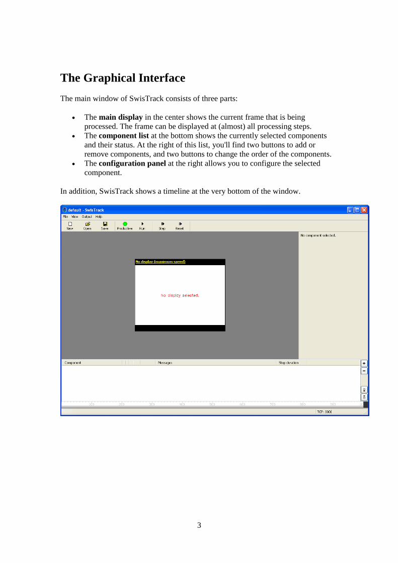
The Graphical Interface
The main window of SwisTrack consists of three parts:
The main display in the center shows the current frame that is being
processed. The frame can be displayed at (almost) all processing steps.
The component list at the bottom shows the currently selected components
and their status. At the right of this list, you'll find two buttons to add or
remove components, and two buttons to change the order of the components.
The configuration panel at the right allows you to configure the selected
component.
In addition, SwisTrack shows a timeline at the very bottom of the window.

4
Editing the Component List
To add a component, click the plus (+) button on the right of the component list. A
dialog will appear and allow you to select a component. Note that the available
components are grouped by their category, and you'll often need a component of each
category, in the order the categories are listed here.
Components are added to the end of your component list. To move them up and
down, use the arrow buttons on the right side. To remove the selected component,
simply click on the minus (-) button.
The component list consists of several columns which indicate the type and the state
of the component. Next to the name of the component, a few columns are filled with
W's, E's and R's. Each of these columns corresponds to a channel (or a data structure),
and the letters have the following meaning:
W: The component is writing to this channel.
E: The component is modifying (reading, then writing) this channel.
R: The component reads from this channel, but doesn't change anything there.
Obviously, you first have to write something to a channel before you can read or
modify it. Hence, if you look through each columns, all E's and R's should be below
the W's. If this isn't the case, then you either forgot to add a component or placed the
components in the wrong order.
In the column right after the component name, you may also see some T's. These
components include a trigger mechanism (which may be active or not), i.e. they tell
SwisTrack when to process the next frame. A setup must have at least one trigger.
Configuring and Testing your Setup
Once your component list contains a valid setup, you can process one frame by
pressing the Step button in the toolbar. This invokes each component in the order they
are listed and displays the selected image (i.e. the output of the selected component).
Once the frame is processed, the component list indicates the duration of each
component, and perhaps error messages. (If you just added some components, it is
quite likely that one or the other component will raise an error. You may have to
configure them first.) Whenever an error occurs, SwisTrack stops the execution of the
frame at that point and doesn't call the subsequent components.
When clicking on a component, SwisTrack displays its configuration panel on the
right side of the window. You can now modify the settings and watch how this affects
the image. Whenever you change a value, SwisTrack automatically performs a step -
hence your modification becomes immediately visible on the screen.
As an advice, start at the top of your component list and configure the components in
the order of execution. As the configuration heavily depends on component itself,
refer to the online component documentation (link on the top of the configuration
panel) for the meaning of each parameter.
5
While the Step button processes one frame, the Run button processes frames
continously. In i>run mode, the trigger components (those with a T next to their
name) say when the next frame shall be processed. If you don't have any trigger
component in your setup, add a Timer Trigger component to configure the processing
speed.
Finally, the Reset button allows you to reset all components. Most of the time,
SwisTrack finds out automatically when the setup must be restarted (especially when
you change the configuration of a component), but there are cases where you want to
that explicitely. When you hit the Reset button, all components are adviced to
completely reset their internal state and reload the configuration. This zeroes the
frame counter and deletes the track history, for example.
Running an Experiment
Once your setup is properly configured and working, you probably want to use it for
your experiments. This is where the Productive button becomes important.
Before you start your experiment, activate the Production button. This resets all
components and starts them in productive mode. At the end of your experiment,
simply hit the Production button again to release it and switch back to testing mode.
Production mode sends the output as designated. When testing outside of production
mode no file will be saved
Productive mode has two main differences as compared to testing mode:
In productive mode, SwisTrack never resets the components automatically.
Therefore, only a subset of the configuration parameters are available any
more, namely those which do not change the processing completely. For
example, you can still adjust the exposure time of a camera, but you cannot
change from color to grayscale mode. In addition, it is not possible to add,
remove or reorder components in productive mode.
Output components only write data to the file during productive mode. Hence,
your the files contain the data of your experiments only. (Some other
components also make slight differences between testing and productive
mode. Refer to the component documentation for details.)
The Timeline
At at the bottom of the main window, SwisTrack displays a timeline with an evolution
of its state (running, not running, productive mode, normal mode) and the frame
processing steps. This not only allows you to see at a glance what Swistrack is doing,
but also to find out where your CPU power is burnt.
By default, SwisTrack records all important events for approximately one second, and
displays them afterwards. Hence, what you see in the timeline corresponds to what
SwisTrack was doing one second ago.
6
Elements on the Timeline
The following elements are drawn on the timeline:
The ruler in the background indicates the milliseconds (ms) from the time
recording of that particular timeline has started.
While SwisTrack is running (Run button pressed), the otherwise white
background changes to light gray.
The lower third of the bar indicates whether SwisTrack is in testing mode
(gray) or productive mode (green).
The blue boxes in the middle represent the steps. Each box corresponds to the
processing time of one component. The box of the selected component is
highlighted in red.
Black vertical lines indicate leap times, but only few components set leap
times.
Components
The following table lists all the General components integrated into SwisTrack:
1) Trigger
2) Input
3) Input Conversion
4) Preprocessing (color)
Preprocessing (grayscale)
Preprocessing (binary)
5) Thresholding (color)
Thresholding (gray)
6) Particle Detection
7) Calibration
8.) Tracking
9.) Output
In this manual I do not describe each of the components, only simply those that I have
experience with or use in current tracking protocols.
1. Triggers
Trigger Timer: Use only when camera does not have an automatic trigger
mechanism. Timer trigger processes frames (in constant intervals) at a given frame
rate.
Trigger Counter: Enables stopping of processing after a certain amount of frames.

7
2. Input
USB Camera
SwisTrack version 4.01 and 4.1 unfortunately only work with USB cameras up to HD
720p (1280 * 720 pixels), and will downscale the image to 640 * 340 pixels, which
though still is rather good. If you try using a full HD (1980 * 1080) you won’t get
anything but a black screen.
We suggest that you use a USB camera with zoom lens since you then can have the
camera a considerable distance away from the arena, and hence minimize the problem
with wide angle lenses. Please only use regular web cams (with rather wide angle
view) for testing and demonstration, or for tracking animals that aren’t moving in the
Z-direction – as e.i. coackroaches.
Fire-wire Camera:
This component allows you to grab image from firewire cameras using the CMU
driver. The output images are grayscale or color (RGB) images. As the CMU driver
does only exist for Windows, this component is not cross platform. The CMU driver
is available from http://www.cs.cmu.edu/~iwan/1394/. This needs to be installed as
the primary Imaging Device driver on your system. Control
Panel>System>Hardware>Device Manager>Imaging Devices (When camera Plugged
in)>Update Driver>…
Camera Number: Allows you to select the camera if there are multiple firewire
cameras connected. Typically 0.
Video Format and Mode: Video Format (0..2) and Mode (0..7) allow you to select
the desired input type from the camera. Beware that a conversion is automatically
done to output only grayscale or RGB images. Thus, YUV format are not really
interesting, except if it allows for an increased camera frame rate.
The table contained within the appendices describes the different modes and formats.
To check the available input types of you camera, you can use the
1394CameraDemo.exe that is included with the CMU driver, or check the camera
datasheet.
Frame Rate: Select the camera frame rate: 1.875 fps (0), 3.75 fps (1), 7.5 fps (2),15
fps (3), 30 fps (4), 60 fps (5), 120 fps (6), 240 fps (7).
To check the available frame rates of you camera, you can use the
1394CameraDemo.exe that is shipped with the CMU driver, or check the camera
datasheet.
8
Configuration Window: Allows you to open a configuration window to modify
other camera parameters of the firewire camera, such as the white balance, saturation,
gain, etc. Note that not all cameras allow you to modify all these parameters.
InputFileAVI:
This component allows you to grab an image from avi video file. The output images
are gray or RGB images.
Compatible formats and codecs are numerous including Mpeg 2,3,4 avi’s, and
H364.avi. Many other formats are useable.
Ensure computer is updated with available codecs, The K-Lite codec pack
(http://www.codecguide.com/) is invaluable when wanting to analyse avi’s.
3. Input Conversion Convert image to either grayscale or RGB. I find Colour conversion more effective
when wanting to use a dynamic background subtraction.
4. Preproccessing Either Colour, Grayscale or Binary depending on your input conversion.
Background subtraction is for subtracting a static image in the form of a bmp file
acquired from the main display of swistrack (right click image, ‘save displayed image
as’). Use mask component to eliminate zones of image not wanting to be tracked.
Background subtraction allows for the subtraction of a static image (i.e. an image of
the tracking arena when the tank does not contain the object destined to be tracked).
From the main display, left click your mouse to bring out the drop down menu, select
‘save displayed image as’ which will save the display image as a .bmp. Select this file
as the background image in the address bar.
Mask
The mask can either be added to the colour or grayscale image (Mask Color or Mask
Grayscale) prior to thresholding, or after thresholding (Mask Binary). Using the same
image saved as the background, open the file in a photo editing programme and black
out areas not wanting to be tracked while whiting out areas where tracking is
intended. By selecting the correct mode (i.e. Black to black for the above example)
you will have blacked out areas not intending to be tracked.
Dynamic Background subtraction is much better if tracking arena is likely to
change, i.e. dirt particles, movement outside tank, reflections on water surface etc. I
find the Grayscale Subtraction clunky and the modes available either produce
shadows on the tracked object presenting a false centre of mass (COM) or tracking of
a negative image. Adaptive background subtraction (colour) is more advanced, and
more accurately tracks moving objects. Subtracting with colour (median) and colour
(mode) appear particularly fruitful. Background subtraction Based on Cheung and

9
Kamath looks great in theory however I have not got this to work. Colour swapper
can be helpful in cleaning up background image. Note, background subtraction
(especially the mode subtraction) can require a lot of the processing requirements.
Elevated requirements can cause camera capture rate to decrease below that set.
Image Erosion and Image Dilation allow you to reduce or expand the pixels that
make up the tracked blob, enabling a larger blob to be tracked. Eroding particles will
help to remove noise, the particle can then be dilated to make for easier tracking.
However, this action may also expand noisy blobs in the thresholded image
potentially adding interfering objects from the background or potentially hide the
object to be tracked .
5. Thresholding
Thresholding (colour or grayscale) allows the user to pull the object intended to be
tracked away from the background. By adjusting the contrast threshold, the desired
object can be pulled out of the image. This moving blob upon the background will
later be the blob selected for tracking.
Thresholding with Individual Threshold values is useful when pulling out objects
to be tracked that are represented by a particular colour. However, the output of this
thresholded colour is a binary (i.e. black/white) blob. This coloured marker, written as
a binary blob, can later be the point selected for tracking. Double thresholding is an
extension of this function whereby a range of a particular colour channel can be
selected for tracking,
6. Particle Detection Particle detection seeks out the moving image from the thresholded image. Blob
detection will select the moving blob from the background. Maximum blobs is the
no. of objects intended to be tracked. Area selection is particularly useful for
separating out the image intended to be tracked from the background and any noise
associated. Orientation and compactness can also be adjusted to filter out the tracked
object from noise when required.
Two coloured marker detection and red-green marker detection functions to
differentiate coloured marks (or leds) from the input image. Again number of particles
is the number of marks on the image wanting to be tracked. Max distance is the
separation of the two marks and is used to filter the marks from potential background
noise. Output selects which of the two marks is the primary mark. Within two colored
marker detection colours can be selected from entering the RGB values of the
intended colour or alternatively from the palette provided within the configuration
panel. Again area and compactness can be limited to reduce interference. Outputs of
the 2 channel marker detection are particularly useful for determining orientations,
calculated within the tracking component and outputted as radians.

10
Circular hough transformation can be used for tracking circular labels or objects,
however, output is again binary.
7. Calibration. No comments included, I typically convert pixels to cm within the output file using
known calibration of camera within experimental setup. (i.e. cm/pixel conversion)
8. Tracking. Nearest Neighbour tracker is the most basic of the components used for tracking the
moving object(s). Number of objects is the intended number of blobs (objects to be
tracked) – This must be the same value as above in Particle detection. The maximum
value slide is a limiter of the expected number of pixels the tracked object will move
between frames. This value needs to be high enough to enable tracking of moving
objects. By selecting an appropriate limitation on the tracked image it will help
prevent track-exchange with other particles on the input.
Other tracking components, filters and smoothers are not typically used when tracking
fish
9. Output. x,y coordinates, area, orientation and compactness as well as a timestamp (ms) can be
output as either a tab delimited .txt file or alternatively sent across a TCP server (port
3000 by default)
The TCP output can be used for analysis in realtime following building of a VI in
Labview or within Matlab.
The .txt file can also be used in real time in programs like Labtech Notebook,
DaisyLab, LabView etc. If tracking just one object the file will contain 9 colums
withtime, x- and y- cooridnates in the first, second and third column.
Finally the .txt file can be used for post analysis in Microsoft Excel. .txt files will
save in a timestamped (ms) folder contained within the same folder that your tracking
protocol is saved within.
If a file is not being saved it is likely the Production button was not pressed while
tracking.
11
10. Appendicies
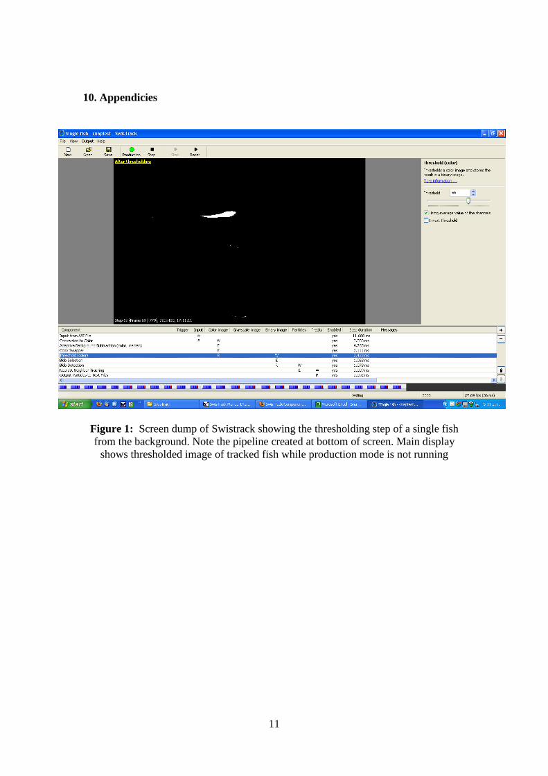
Figure 1: Screen dump of Swistrack showing the thresholding step of a single fish
from the background. Note the pipeline created at bottom of screen. Main display
shows thresholded image of tracked fish while production mode is not running

12
(i)
(ii)
(iii)
Figure 2: Steps towards masking a static background. (i) .bmp image of tracking
arena. (ii) Blacked out zone not wanting to be tracked (iii) Superimposed masked area
on a (poorly) thresholded input image

13
Figure 3: Screen dump of Swistrack actively tracking multiple fish. Main display
shows output of tracked fish while production mode is not running. Note, multiple
fish tracking by this protocol experiences track exchange when fish cross
11:
A few benefits with SwisTrack:
A: Work in real-time w inexpensive USB cameras – and make feed-back on the target
possible.
B: Target strength discrimination: One very usefull and strong feature in
SwisTrack is that you can selecet approximately how large (number of pixels) your
target is. Hence pixel noice caused by e.i. the animal defecating during the experiment
will be ingnored in the calculation of the X- Y coordinate mass midpoint.
C: 3D-tracking of one fish: Another very usefull feature in SwisTrack is that you can
track e.i. a fish in 3D by having the fish in a gals aquariaum and e.i having the camera
above for the X- and Y- coordinate, and a mirror at an angle of 45 Deg so the same
camera in addition to the view from above will montor the aquarium from the side. By
tracking the fish as two objects one rcak will be equal to the X and Y- coorinates, and
the other the Z- and X- or Y coordinate.

14
Fig 1.Left:
Experimental setup for 3D tracking of one zebrafish. A: camera. B: aquarium. E
and D: mirrors. F. Light source. H. Computer.
Fig 1. Right:
Images of one fish – B is vertical view (X- and Y- coordinates) and D is
horizontal view through mirror D.
(H. Bergsson, B. Sc.-theis unpublished).
Fig. 2 SwisTrack derived 3D track of zebrafish using one camera and two
mirrors. (H. Bergsson, B.Sc.-thesis unpublished).

15
Table 1: Firewire camera settings when using CMU driver for selection within
configuration panel of Input from Firewire (1394) camera Offset Name Field Bit Description
180h V_MODE_INQ_0 Mode_0 [0] 160 X 120 YUV(4:4:4) Mode
(24bit/pixel)
(Format_0) Mode_1 [1] 320 X 240 YUV(4:2:2) Mode
(16bit/pixel)
Mode_2 [2] 640 X 480 YUV(4:1:1) Mode
(12bit/pixel)
Mode_3 [3] 640 X 480 YUV(4:2:2) Mode
(16bit/pixel)
Mode_4 [4] 640 X 480 RGB Mode (24bit/pixel)
Mode_5 [5] 640 X 480 Y (Mono) Mode (8bit/pixel)
Mode_6 [6] 640 X 480 Y (Mono16) Mode
(16bit/pixel)
184h V_MODE_INQ_1 Mode_0 [0] 800 X 600 YUV(4:2:2) Mode
(16bit/pixel)
(Format_1) Mode_1 [1] 800 X 600 RGB Mode (24bit/pixel)
Mode_2 [2] 800 X 600 Y (Mono) Mode (8bit/pixel)
Mode_3 [3] 1024 X 768 YUV(4:2:2) Mode
(16bit/pixel)
Mode_4 [4] 1024 X 768 RGB Mode (24bit/pixel)
Mode_5 [5] 1024 X 768 Y (Mono) Mode (8bit/pixel)
Mode_6 [6] 800 X 600 Y (Mono16) Mode
(16bit/pixel)
Mode_7 [7] 1024 X 768 Y (Mono16) Mode
(16bit/pixel)
188h V_MODE_INQ_2 Mode_0 [0] 1280 X 960 YUV(4:2:2) Mode
(16bit/pixel)
(Format_2) Mode_1 [1] 1280 X 960 RGB Mode (24bit/pixel)
Mode_2 [2] 1280 X 960 Y (Mono) Mode (8bit/pixel)
Mode_3 [3] 1600 X 1200 YUV(4:2:2) Mode
(16bit/pixel)
Mode_4 [4] 1600 X 1200 RGB Mode (24bit/pixel)
Mode_5 [5] 1600 X 1200 Y (Mono) Mode (8bit/pixel)
Mode_6 [6] 1280 X 960 Y (Mono16) Mode
(16bit/pixel)
Mode_7 [7] 1600X 1200 Y (Mono16) Mode
(16bit/pixel)
18ch
... Reserved for other
V_MODE_INQ_x
for Format_x.
198h V_MODE_INQ_6 Mode_0 [0] Exif format
(Format_6) Mode_x [1...7] Reserved for another Mode
- [8..31] Reserved
19ch V_MODE_INQ_7 Mode_0 [0] Format_7 Mode_0
(Format_7) Mode_1 [1] Format_7 Mode_1
Mode_2 [2] Format_7 Mode_2
Mode_3 [3] Format_7 Mode_3
Mode_4 [4] Format_7 Mode_4
Mode_5 [5] Format_7 Mode_5
Mode_6 [6] Format_7 Mode_6
Mode_7 [7] Format_7 Mode_7

16
References concerning SwisTrack:
Correll, N., Sempo, G., Lopez de Meneses, Y. Halloy, J., Deneubourg, J.-L. and
Martinoli, A. SwisTrack: A Tracking Tool for Multi-Unit Roboticand Biological
Systems.(2008). Proceedings of the 2006 IEEE/RSJInternational Conference on
Intelligent Robots and SystemsOctober 9 - 15, 2006, Beijing, China
Lochmatter, T., Roduit, P., Cianci, C., Correll, N., Jacot, J. and Martinoli, A. (2008).
SwisTrack - A Flexible Open Source Tracking Software for Multi-
AgentSystems.IEEE/RSJ International Conference on Intelligent Robots and
SystemsAcropolis Convention CenterNice, France, Sept, 22-26, 2008.
References concerning what it can be used for in biological systems:
Example of post experimental analysis:
Cook, D.G., Brown, E., Lefevre, S., Domenici, P. and Steffensen, J. F. (2014). The
response of striped surfperch Embiotoca lateralis to progressive hypoxia: Swimming
activity, shoal structure, and estimated metabolic expenditure. J. Exp. Mar. Biol. Ecol.
460, 162-169
Link to Research gate project page with description of how to use Swistrack in a
temperature shuttlebox system:
"Steffensen" shuttle box for temperature preference - how to build and run it:
originally described in:
Schurmann, H., Steffensen, J. F., Lomholt, J. P. (1991). The influence of hypoxia on
the preferred temperature of rainbow-trout, Oncorhyncus mykiss. J. exp. Biol. 157:
75-86.
Schurmann, H. & Steffensen, J. F. (1992). Lethal oxygen levels at different
temperatures and the preferred temperature during hypoxia of the Atlantic cod, Gadus
morhua. J. Fish. Biology, 41;927-934.
Schurmann, H. & Steffensen, J. F. (1994). Spontaneous activity of Atlantic cod,
Gadus morhua, exposed to graded hypoxia at three different temperatures. J. exp.
Biol. 197; 129-142.
View publication statsView publication stats