swift/uvot+manga (swim) value-added catalog
TRANSCRIPT

Draft version September 23, 2020Typeset using LATEX twocolumn style in AASTeX62
Swift/UVOT+MaNGA (SwiM) Value-added Catalog
Mallory Molina,1, 2 Nikhil Ajgaonkar,3 Renbin Yan,3 Robin Ciardullo,1 Caryl Gronwall,1
Michael Eracleous,1 Xihan Ji,3 and Michael R. Blanton4
1Department of Astronomy and Astrophysics and Institute for Gravitation and the Cosmos, The Pennsylvania State University, 525Davey Lab, University Park, PA 16803, USA
2eXtreme Gravity Institute, Department of Physics, Montana State University, Bozeman, MT 59715, USA3Department of Physics and Astronomy, University of Kentucky, 505 Rose St., Lexington, KY 40506-0057, USA
4Center for Cosmology and Particle Physics, Department of Physics, New York University
ABSTRACT
We introduce the Swift/UVOT+MaNGA (SwiM) value added catalog, which comprises 150 galaxies
that have both SDSS/MaNGA integral field spectroscopy and archival Swift/UVOT near-UV (NUV)
images. The similar angular resolution between the three Swift/UVOT NUV images and the MaNGA
maps allows for a high-resolution comparison of optical and NUV indicators of star formation, crucial
for constraining quenching and attenuation in the local universe. The UVOT NUV images, SDSS
images, and MaNGA emission line and spectral index maps have all been spatially matched and re-
projected to match the point spread function and pixel sampling of the Swift/UVOT uvw2 images, and
are presented in the same coordinate system for each galaxy. The spectral index maps use the definition
first adopted by Burstein et al. (1984), which makes it more convenient for users to compute spectral
indices when binning the maps. Spatial covariance is properly taken into account in propagating the
uncertainties. We also provide a catalog that includes PSF-matched aperture photometry in the SDSS
optical and Swift NUV bands. In an earlier, companion paper (Molina et al. 2020) we used a subset
of these galaxies to explore the attenuation laws of kiloparsec-sized star forming regions. The catalog,
maps for each galaxy, and the associated data models, are publicly released on the SDSS websitea).
Keywords: galaxies: general – astronomy data analysis – catalogs – photometry: Sloan – photometry:
ultraviolet – spectroscopy
1. INTRODUCTION
The growth and quenching of star formation within
a galaxy are central elements of galaxy evolution. In
order to fully understand this process, the appropriate
methodological tools and physical models must be in
place, including an accurate attenuation law and star
formation quenching models. The former is dictated by
the intrinsic properties of the regions studied, such as
the star formation rate (SFR), stellar mass-specific SFR
(log[SFR/M∗]) and the chosen sightline, all of which
change across the face of the galaxy (e.g., Charlot &
Fall 2000; Calzetti et al. 2000; Wild et al. 2011; Xiao
et al. 2012; Battisti et al. 2016; Salim et al. 2018). Sim-
ilarly, the physical mechanisms that drive the quench-
Corresponding author: Nikhil Ajgaonkar
a) https://data.sdss.org/sas/dr16/manga/swim/v3.1/
ing of star formation could be constrained by its spatial
progression within a galaxy. For example, both mor-
phological quenching and feedback from active galactic
nuclei (AGN) produce inside-out quenching (with differ-
ent timescales; Martig et al. 2009; Springel et al. 2005),
while mechanisms such as ram-pressure stripping (Stein-
hauser et al. 2016) would produce outside-in quenching.
Therefore, spatially resolved measurements of the re-
cent star formation history (SFH) across the faces of
galaxies are necessary to study quenching in galaxies.
The near ultra-violet (NUV) band and the nebular Hα
recombination line are robust SFR indicators that probe
different timescales (∼ 100 Myr for NUV, and ∼ 10 Myr
for Hα, see Kennicutt 1998; Kennicutt & Evans 2012;
Calzetti 2013, for details). Combined with other stellar
continuum features, they can provide constraints on the
spatial progression of quenching. They are also crucial
to understanding the relevant attenuation law in star
forming regions, including the strength and contribution
arX
iv:2
007.
0854
1v4
[as
tro-
ph.G
A]
21
Sep
2020

2
of the 2175 A bump (e.g., Calzetti et al. 2000; Battisti
et al. 2016, 2017; Molina et al. 2020).
The high spatial resolution and narrow NUV filters
required for the study of the quenching of star forma-
tion are not attainable with the single broad NUV fil-
ter and 5′′ angular resolution of the Galaxy Evolution
Explorer (GALEX; Martin et al. 2005). Therefore,
we constructed a catalog of galaxies with Sloan Digi-
tal Sky Survey IV (SDSS-IV) Mapping Nearby Galaxies
at Apache Point Observatory (MaNGA; Bundy et al.
2015; Yan et al. 2016; Blanton et al. 2017) optical inte-
gral field unit (IFU) spectroscopy and archival Swift Ul-
traviolet Optical Telescope (UVOT; Roming et al. 2005)
NUV images. The similar angular resolution (∼ 2.′′5) of
Swift/UVOT and SDSS-IV/MaNGA provides a view of
nearby galaxies in both the NUV and optical bands at
a spatial resolution of order 1 kpc.
The combination of the spatially-matched NUV im-
ages and optical IFU maps creates a powerful dataset
that can address a number of astrophysical questions.
We have used a subset of the galaxies in this catalog
in Molina et al. (2020)1 to explore the relevant attenua-
tion law for kiloparsec-sized star forming regions. Future
work will include using the spectral information to test
models of galaxies where star formation is being or has
recently been extinguished.
We discuss the sample selection for the Swift+MaNGA
(SwiM) catalog and its basic properties in Section 2, and
detail the Swift/UVOT and MaNGA data reduction in
Section 3. The integrated photometric measurements
are described in 4. The process of spatial matching be-
tween Swift and SDSS images and MaNGA IFU spec-
troscopy is presented in Section 5. We discuss the AGN
fraction of the sample in Section 6 and provide notes
about individual objects in Section 6.2. We summarize
in Section 7. We assume a ΛCDM cosmology when quot-
ing masses, distances, and luminosities, with Ωm = 0.3,
Λ = 0.7 and H0 = 70 km s−1 Mpc−1.
2. THE SwiM CATALOG
2.1. SDSS-IV/MaNGA and Swift/UVOT
Our sample of galaxies is a subset of the MaNGA sur-
vey (Bundy et al. 2015; Yan et al. 2016), which is a spa-
tially resolved optical IFU spectroscopic survey included
in the fourth generation of SDSS (SDSS-IV; Blanton
1 Molina et al. (2020) used a previous version of the data re-duction presented here, which does not include errors due to co-variance or matching the Swift/UVOT images to the resolutionof the uvw2 filter. Additionally, the Dn(4000) error bars in thatversion were overestimated by including a factor of 1.98 for cali-bration uncertainties instead of 1.4. However, none of these issuesaffected the results presented in that work.
et al. 2017). The main sample of the MaNGA survey
will have ∼ 10, 000 galaxies that (1) create a uniform
distribution in stellar mass for M∗ > 109 M, as ap-
proximated via the SDSS i-band absolute magnitude,
(2) provide uniform spatial coverage in units of half-light
radius (Re), and (3) maximize the spatial resolution and
signal-to-noise for each galaxy (Wake et al. 2017). This
work uses the MaNGA Product Launch 7 (MPL-7) ver-
sion of the MaNGA sample, which includes all objects
observed by June 2017, totaling 4706 galaxies.
The MaNGA data were taken with hexagonal IFU
fiber bundles that contain between 19 and 127 2′′ fibers,
extending over a diameter of between 12′′ and 32′′
(Drory et al. 2015). The fiber bundles are inserted
into pre-drilled holes on plates mounted on the Sloan
2.5-m telescope (Gunn et al. 2006), and fed into the
dual-channel Baryon Oscillation Spectroscopic Survey
(BOSS) spectrographs (Smee et al. 2013). The BOSS
spectrograph is designed with red and blue arms in or-
der to provide continuous wavelength coverage from the
NUV to near-IR. Therefore the MaNGA spectra span
the wavelength range 3, 622–10, 350 A with a resolving
power of R ∼ 2000, allowing for the use of most nebu-
lar diagnostics, including BPT diagrams (Baldwin et al.
1981). The telescope is dithered to achieve near-critical
sampling of the point spread function (PSF), which has
been measured at 2.′′5, while the resulting data cubes
have a spatial sampling of 0.′′5. The total exposure
time for each object is set by the sum of the squared
signal-to-noise ratio: the sum of (S/N)2 must be at least
20 pixel−1 fiber−1 in the g-band at galactic-extinction-
corrected g = 22 AB mag, and 36 pixel−1 fiber−1 in the
i-band at galactic-extinction-corrected i = 21 AB mag.
These criteria result in an average integration time of
2.5 hours (Yan et al. 2016).
In order to probe both NUV and optical properties,we also make use of Swift/UVOT photometry. UVOT is
a 30-cm telescope with a field of view (FoV) of 17′×17′,
an effective plate scale of 1′′ pixel−1, and three NUV
filters: uvw2, uvm2 and uvw1 (Roming et al. 2005).
While the UVOT PSF varies with wavelength (see Ta-
ble 1), all three filters give a resolution around 2.′′5, i.e.,
similar to the angular resolution of the MaNGA optical
spectra. The detector in the UVOT is a microchannel
plate intensified CCD that operates in a photon count-
ing mode, which can cause bright sources to suffer from
coincidence loss (Poole et al. 2008; Breeveld et al. 2010).
However, as discussed in Section 3.3, the galaxies in our
sample are too faint for this to be a significant problem.
2.2. The Cross-matched Catalog

3
Table 1. Swift/UVOT NUV Observation Properties
Central Spectral PSF Median Minimum Faintest
Wavelengtha,b FWHMa FWHMa Exposure Exposure Magnituded
Filter (A) (A) (arcsec) (s) (s) (mAB)
uvw2 1928 657 2.92 2375 187 22.3
uvm2c 2246 498 2.45 2093 166 22.3
uvw1 2600 693 2.37 1658 120 21.1
aAll filter properties are from Breeveld et al. (2010).b The central wavelength assumes a flat spectrum in fν .c The uvm2 exposure time statistics only include galaxies with uvm2 im-
ages.
dThe faintest magnitude in our data set for each filter.
We constructed our sample by cross-referencing the
MPL-7, i.e., the SDSS Data Release 15 (DR15) (Aguado
et al. 2019), with the Swift/UVOT NUV archive as of
April 2018. The UVOT archive is a combination of
stars, active and normal galaxies, and gamma ray burst
sources. The objects included in this sample are not al-
ways targeted, but instead fall within the FoV of UVOT.
We required all objects to have usable, science-ready
data cubes from MaNGA and have uvw1 and uvw2 ob-
servations in the Swift/UVOT archive. We do not re-
quire uvm2 data for inclusion in the sample. Using these
criteria, we obtained a sample of 150 galaxies, 87% of
which have uvm2 observations. We report the UVOT
properties, and exposure time statistics, and the faintest
magnitude detected in each filter in Table 1.
The basic properties of the SwiM catalog galaxies, in-
cluding the SDSS classification from DR15 (see Bolton
et al. 2012, for details), derived quantities, and observa-
tion information from MANGA and UVOT, are stored
in a table available in its entirety in the electronic edi-
tion of the Astrophysical Journal. We show the format
for this table in Table 3 in Appendix A.1, and the data
model for the spatially-matched maps in Tables 4–9 in
Appendix A.2. 57% of the sample have either “Galaxy”
or no available SDSS classification, while 31% are classi-
fied as star-forming, 8% as AGN and 4% as starbursts.
The median redshift is 0.033, which corresponds to a
luminosity distance of 134.3 Mpc, and a spatial scale of
0.6 kpc/′′. The stellar masses of the galaxies are pro-
vided by the NASA Sloan Atlas catalog (NSA; Blan-
ton et al. 2011) v1 0 1 based on the aperture-corrected
elliptical-Petrosian photometry (for details see Wake
et al. 2017). The stellar masses for this SwiM sample are
in the range 8.73 ≤ log(M∗/M) ≤ 11.11, with a me-
dian of log(M∗/M) = 10.02. The SFRs are calculated
by the MaNGA Data Analysis Pipeline (Westfall et al.
2019) from the Hα emission line flux within one effective
radius, 1 Re, via the scaling relation given in Kennicutt
& Evans (2012), after an internal reddening correction
assuming the O’Donnell (1994) extinction law. The re-
sulting SFRs span 0 . SFR(Hα) . 25 M yr−1, with a
median value of 0.18 M yr−1.
2.3. Comparison of SwiM catalog to MaNGA
The MaNGA main sample is the combination of three
different subsamples: Primary, Secondary, and Color-
Enhanced samples (Wake et al. 2017). The catalog pre-
sented here contains 63 objects from the Primary sam-
ple, 57 from the Secondary sample, and 31 from the
Color-Enhanced sample. Therefore, while these individ-
ually defined samples from MaNGA can be combined in
different configurations, we compare the SwiM catalog
to the combination of all three, i.e., the “MaNGA main
sample” as defined in MPL-7.
We compare the distributions of redshift, g − r color,
size, and axial ratio of SwiM catalog galaxies to those of
the MaNGA main sample in Figure 1. The size is probed
by the elliptical Petrosian half-light semi-major axis de-
fined in the r-band, and all plotted quantities are taken
from the NASA-Sloan Atlas. The majority of our galax-
ies fall within the range z . 0.05, RPet,50 < 20′′, and
b/a & 0.6. The distributions of redshift, RPet,50 and b/a
in the SwiM catalog are similar to that of the MaNGA
main sample. We also show the distributions of stellar
mass, the SFR and the “star-forming main sequence,”
i.e., the SFR (as given by Hα within 1Re) vs. stellar
mass for our catalog as compared to the full MaNGA
sample in Figure 2. The majority of our galaxies fall
within the range of log(M∗/M) & 9.5. The reduced
MaNGA emission-line flux maps are already corrected
for foreground Milky Way extinction, but not for inter-
nal attenuation in the target galaxy. While this can be
complicated in the UV, most attenuation curves agree
at redder wavelengths including Hα. We therefore as-sume the O’Donnell (1994) law, along with an intrin-
sic Hα/Hβ ratio of 2.86 (Osterbrock & Ferland 2006,
chapter 11), and correct both the MaNGA main sample
and the SwiM catalog for internal attenuation. The cor-
rected SFRs are shown in both the top right and bottom
panels of Figure 2. The SwiM catalog generally recov-
ers the star forming main sequence seen in the MaNGA
sample, but is overly populated at the low-mass, low-
SFR end, and sparsely populated relative to MaNGA at
the high-mass, high-SFR end. This trend is also quali-
tatively seen in the SFR 1–D histogram on the top right
of Figure 2.
2.4. Correction Factors to Volume-Limited Weights
The MaNGA sample was selected to have a flat num-
ber density distribution with respect to the stellar mass
(as approximated by the SDSS i-band magnitude) and

4
0.00 0.05 0.10 0.15Redshift
0.00
0.05
0.10
0.15
0.20
0.25
0.30
Norm
alize
dN
um
ber
of
Gala
xie
s MaNGA Main Sample
SwiM Sample
0.0 0.2 0.4 0.6 0.8 1.0g − r
0.0
0.1
0.2
0.3
0.4
Norm
alize
dN
um
ber
of
Gala
xie
s
0 5 10 15 20RPet,50 (arcsec)
0.0
0.1
0.2
0.3
0.4
Norm
alize
dN
um
ber
of
Gala
xie
s
0.2 0.4 0.6 0.8 1.0b/a (Axis Ratio)
0.00
0.05
0.10
0.15
0.20
0.25
0.30
Norm
alize
dN
um
ber
of
Gala
xie
s
Figure 1. Distribution of the redshift, g−r color, Petrosian half-light radius (derived from r-band photometry), and the r-bandaxis ratio (b/a) of the galaxies in the SwiM catalog as compared to the MaNGA main sample. All histograms are normalizedby the total number of galaxies in each data set. In each panel, the blue dashed outline represents the distribution of the SwiMcatalog, while the gray shaded region represents the MaNGA main sample. The SwiM catalog has a similar distribution to theMaNGA main sample for all four properties. We perform a quantitative comparison of the two data sets in Section 2.4. Alldata were taken from the NASA-Sloan Atlas.
thus cannot be described as magnitude- or volume-
limited. Wake et al. (2017) have provided weights for
each MaNGA target that will statistically correct the
sample to that of a volume-limited data set. If our cata-
log is consistent with a random sampling of the MaNGA
main sample, then the weights calculated by Wake et al.
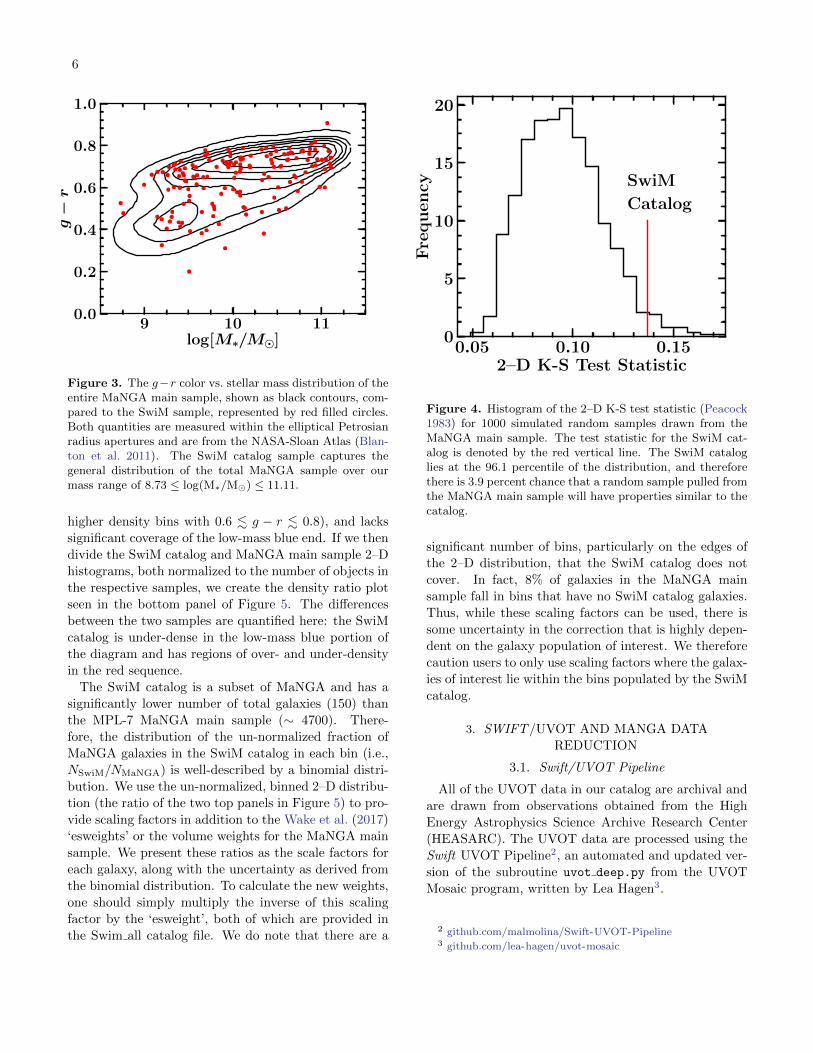
(2017) should be applicable. We show the g− r vs. stel-
lar mass distribution of the entire MaNGA sample as
black contours, with the SwiM catalog overlaid as red
points in Figure 3. While we sample a large portion
of the parameter space, we do not have an even sam-
pling of the MaNGA catalog in the color-mass space.
We test for a quantitative similarity between our cata-
log and a random sample of the same size pulled from
the MaNGA distribution using the 2–D K-S test (Pea-
cock 1983). Specifically, we create 1000 samples of 150
galaxies randomly drawn from the MaNGA main sam-
ple and compare the resulting 2–D K-S test statistic be-
tween that sample and the MaNGA main sample. We
show the distribution of the test statistic, along with
the measured test statistic for the SwiM catalog in Fig-
ure 4; the test statistic is defined such that a larger
value denotes a lower probability that the two distri-
butions are quantitatively similar in the observed 2–D

5
9 10 11log(M∗/M)
0.0
0.1
0.2
0.3
0.4
0.5
0.6
Norm
alize
dN
um
ber
of
Gala
xie
s
−4 −3 −2 −1 0 1log[SFR1Re
[Hα]/(M yr−1)]
0.00
0.05
0.10
0.15
0.20
0.25
0.30
Norm
alize
dN
um
ber
of
Gala
xie
s
MaNGA Main Sample
SwiM Sample
9 10 11log[M∗/M]
−4
−3
−2
−1
0
1
log[S
FR
1R
e[Hα
]/(M
yr−
1)]
Figure 2. Top Left: Same as Figure 1, but for stellar mass. The SwiM catalog has an over density of low-mass objects comparedto the MaNGA main sample. Top Right: Same as Figure 1, but for the SFR(Hα) within 1Re. The L(Hα) measurements havebeen corrected for foreground extinction and internal attenuation in both catalogs, assuming the O’Donnell (1994) law andRV = 3.1. The SwiM catalog has an over density of low-SFR objects, and an under density of high-SFR objects compared tothe MaNGA main sample. Bottom: SFR(Hα) within 1Re vs. stellar mass for the SwiM catalog as compared to the full MaNGAsample. The L(Hα) measurements have been corrected for internal attenuation as described above. The catalog recovers thegeneral distribution, except for the high-mass, high-SFR end of the star forming main sequence.
parameter space. We find that the SwiM catalog lies at
the 96.1 percentile of the distribution presented in Fig-
ure 4, and therefore there is only a ∼ 4% chance that
a random sample pulled from the MaNGA main sample
would have properties similar to the SwiM catalog. We
therefore conclude that there are some selection effects
that make the SwiM catalog different from a randomly-
drawn sample and the Wake et al. (2017) weights must
be scaled in order to statistically correct our catalog to
that of a volume-limited sample.
In order to quantify those scaling corrections, we
binned both the SwiM catalog and the MaNGA main
sample using a linearly spaced, 10 × 10 binning scheme
in the g− r vs. stellar mass space as shown in Figure 5.
When plotted this way, the difference between the two
data sets become obvious: the MaNGA main sample has
a strong peak in the high-mass red end of the diagram
with a second weaker peak at the low-mass, blue end
of the diagram. Meanwhile the SwiM catalog samples
the red sequence in a different way (i.e., the band of
6
9 10 11log[M∗/M]
0.0
0.2
0.4
0.6
0.8
1.0
g−r
Figure 3. The g−r color vs. stellar mass distribution of theentire MaNGA main sample, shown as black contours, com-pared to the SwiM sample, represented by red filled circles.Both quantities are measured within the elliptical Petrosianradius apertures and are from the NASA-Sloan Atlas (Blan-ton et al. 2011). The SwiM catalog sample captures thegeneral distribution of the total MaNGA sample over ourmass range of 8.73 ≤ log(M∗/M) ≤ 11.11.
higher density bins with 0.6 . g − r . 0.8), and lacks
significant coverage of the low-mass blue end. If we then
divide the SwiM catalog and MaNGA main sample 2–D
histograms, both normalized to the number of objects in
the respective samples, we create the density ratio plot
seen in the bottom panel of Figure 5. The differences
between the two samples are quantified here: the SwiM
catalog is under-dense in the low-mass blue portion of
the diagram and has regions of over- and under-density
in the red sequence.The SwiM catalog is a subset of MaNGA and has a
significantly lower number of total galaxies (150) than
the MPL-7 MaNGA main sample (∼ 4700). There-
fore, the distribution of the un-normalized fraction of
MaNGA galaxies in the SwiM catalog in each bin (i.e.,
NSwiM/NMaNGA) is well-described by a binomial distri-
bution. We use the un-normalized, binned 2–D distribu-
tion (the ratio of the two top panels in Figure 5) to pro-
vide scaling factors in addition to the Wake et al. (2017)
‘esweights’ or the volume weights for the MaNGA main
sample. We present these ratios as the scale factors for
each galaxy, along with the uncertainty as derived from
the binomial distribution. To calculate the new weights,
one should simply multiply the inverse of this scaling
factor by the ‘esweight’, both of which are provided in
the Swim all catalog file. We do note that there are a
0.05 0.10 0.152–D K-S Test Statistic
0
5
10
15
20
Fre
qu
en
cy SwiM
Catalog
Figure 4. Histogram of the 2–D K-S test statistic (Peacock1983) for 1000 simulated random samples drawn from theMaNGA main sample. The test statistic for the SwiM cat-alog is denoted by the red vertical line. The SwiM cataloglies at the 96.1 percentile of the distribution, and thereforethere is 3.9 percent chance that a random sample pulled fromthe MaNGA main sample will have properties similar to thecatalog.
significant number of bins, particularly on the edges of
the 2–D distribution, that the SwiM catalog does not
cover. In fact, 8% of galaxies in the MaNGA main
sample fall in bins that have no SwiM catalog galaxies.
Thus, while these scaling factors can be used, there is
some uncertainty in the correction that is highly depen-
dent on the galaxy population of interest. We therefore
caution users to only use scaling factors where the galax-
ies of interest lie within the bins populated by the SwiM
catalog.
3. SWIFT/UVOT AND MANGA DATA
REDUCTION
3.1. Swift/UVOT Pipeline
All of the UVOT data in our catalog are archival and
are drawn from observations obtained from the High
Energy Astrophysics Science Archive Research Center
(HEASARC). The UVOT data are processed using the
Swift UVOT Pipeline2, an automated and updated ver-
sion of the subroutine uvot deep.py from the UVOT
Mosaic program, written by Lea Hagen3.
2 github.com/malmolina/Swift-UVOT-Pipeline3 github.com/lea-hagen/uvot-mosaic

7
8 9 10 11 12log[M∗/M]
0.0
0.2
0.4
0.6
0.8
1.0
g−r
MaNGA
0
100
200
300
400
Nu
mb
er
of
Gala
xie
s8 9 10 11 12
log[M∗/M]
0.0
0.2
0.4
0.6
0.8
1.0
g−r
SwiM
0
2
4
6
8
10
12
14
16
Nu
mb
er
of
Gala
xie
s
8 9 10 11 12log[M∗/M]
0.0
0.2
0.4
0.6
0.8
1.0
g−r
0.0
0.5
1.0
1.5
2.0
2.5
3.0
(nS
wiM/n
MaN
GA)
Figure 5. 2–D histograms of the number distribution of the MPL-7 MaNGA main sample (top left) and the SwiM catalog(top right), and the ratio between the two (bottom center), in g − r vs. stellar mass. The two sample distributions on thetop show high density as yellow, and low density as shades of purple, denoted by the color bar. The MaNGA main samplehas a strong peak in the high-mass portion of the red sequence and a secondary peak in the low-mass, blue portion of thediagram. Meanwhile the SwiM catalog samples the red sequence in a different way and includes a smaller fraction of low-massblue galaxies. The bottom shows the ratio of the number densities of the SwiM catalog (nSwiM) and the MaNGA main sample(nMaNGA). Both number densities are calculated by normalizing to the total number of objects in each sample (150 and 4498,respectively). If the number densities are equal, the bin color is white, while over-densities in the SwiM catalog are representedby shades of red and under-densities by shades of blue, as denoted by the color bar. The qualitative number density differencesbetween the two catalogs seen in the top two panels are quantified here.

8
The uvot deep.py subroutine reads in data already
downloaded from HEASARC, and follows the basic data
processing procedures for UVOT images as described in
the UVOT Software Guide4 as described below. The
program ensures that both the counts and exposure
maps are aspect corrected, reducing the uncertainty in
the defined world coordinate system to 0.′′5. Occasion-
ally uvot deep.py will produce errors that cause the
exposure map to have 0 or NaN values for small regions
of pixels. This error only occurs in 5 galaxies out of
the 150 galaxy sample. Furthermore, the error is only
present within the galaxy itself for two objects. We pro-
vide masks to correct for this issue, which is described
in Appendix A.1.
All UVOT images are mosaics of single frames with
very short exposures that are stacked together to pro-
duce a deep image. UVOT does allow for different
frame exposure times according to the science goal of
the observation. However, the UVOT software will
not combine frames with different frame times, as
this would greatly complicate the analysis. Currently
uvot deep.py requires the standard full frame exposure
time of 11.0322 ms for inclusion in the final image. Ad-
ditionally, all individual frames must be 2 × 2 binned,
yielding a plate scale of 1′′ pixel−1. If an individual
frame meets both of these requirements and is aspect
corrected, then it is added to the final image. As both
criteria are standard for non-event mode data, we re-
tain the majority of frames in this process. The final
counts and exposure maps are corrected for large scale
structure (see Breeveld et al. 2010, for details) and have
all bad pixels masked.
The Swift UVOT Pipeline automates uvot deep.py,
and will reduce multiple Swift images in a single exe-
cution. In one run, the pipeline will parse data already
downloaded from HEASARC and run a modified ver-
sion of uvot deep.py. This modified version will align
the large scale structure correction map (if needed), skip
any image that does not meet the requirements of the
original uvot deep.py, and store that information in a
log file for reference. This process is then repeated for
each image of interest.
The distribution of exposure times for the Swift/UVOT
NUV observations are shown in Figure 6. The majority
of objects have exposure times of less than 5000 s in
all three filters, with the median exposure time listed
in Table 1. The limiting visual magnitude for a 5σ de-
tection for a 5 ks observation is mV = 22.45 for uvw2,
mV = 22 for uvm2, and mV = 22.2 for uvw1. Addition-
4 heasarc.gsfc.nasa.gov/docs/swift/analysis
0 5 10 15 20 25Swift Exposure Time (ks)
0
10
20
30
40
50
60
70
Nu
mb
er
of
Gala
xie
s
uvw2
uvm2
uvw1
Figure 6. The distribution of exposure times for eachSwift/UVOT filter in kiloseconds. The exposure time dis-tribution for uvw2 is shown in as the grey filled histogram,while that of uvm2 and uvw1 are shown in dashed blue andsolid red lines, respectively. The majority of exposures in allthree filters are less than 5 ks. The minimum visual magni-tudes for a 5σ detection are listed in Section 3.1.
ally, the limiting visual magnitude for each filter, given
their respective median exposures, are mV = 22.04 for
uvw2, mV = 21.53 for uvm2, and mV = 21.6 for uvw1.
3.2. Further UVOT Data Processing
After the images are processed through the Swift
UVOT Pipeline, they are corrected for both the dead
time and degradation of the detector. The UVOT detec-
tor is a microchannel plate intensified CCD, operating
in a photon counting mode. As a result, approximately
2% of the full frame time is dedicated to transferring
charge out of the detector. This is corrected by increas-
ing the count rate (Poole et al. 2008). Meanwhile, the
decline in count rate due to the degradation of the de-
tector is well characterized and provided in the UVOT
calibration documents5; this results in a 2.5% correction
for the most recent observations.
Cosmic ray corrections are not necessary for UVOT
images, due to its operation mode. For each ∼ 11 ms
frame, all individual events are identified, and the cen-
troid of the event location is saved. When the final im-
age is created, each event is recorded as a count, with its
location on the image given by the calculated centroid
described above. In this regime, a cosmic ray that hits
the detector will register at most a few counts in a sin-
5 heasarc.gsfc.nasa.gov/docs/heasarc/caldb/swift/docs/uvot

9
gle location, while a stationary astrophysical source will
register thousands of counts. Therefore cosmic rays are
incorporated into the background counts as they affect
very few frames.
3.3. Coincidence Loss in Swift/UVOT Images
Coincidence loss occurs when two or more photons ar-
rive at a similar location within the same ∼ 11 ms frame,
causing a pile-up that affects the measured count rate.
As UVOT operates in a photon-counting mode, this be-
comes a significant issue for bright sources. Poole et al.
(2008) characterized this effect for a single-pixel detec-
tor, while Breeveld et al. (2010) describe coincidence loss
when a point source is in front of a diffuse background
(e.g., knots of star formation on top of a galaxy). Thus
the Breeveld et al. (2010) model appears to be the most
appropriate for our data set.
However, in order to avoid PSF variation in individual
filters, Breeveld et al. (2010) recommended a minimum
aperture size of 3′′ for all the three NUV filters, corre-
sponding to a physical size of ∼ 1.8 kpc for the median
redshift of our sample. With such an aperture, we can-
not resolve individual H II regions which have typical
sizes of no more than a few hundred parsecs (Kennicutt
1984; Garay & Lizano 1999; Kim & Koo 2001; Hunt &
Hirashita 2009). Therefore, the point source plus diffuse
background model described by Breeveld et al. (2010) is
not appropriate.
Instead we approach this problem in the spirit of
Poole et al. (2008). The formulated coincidence loss
corrections are only valid for point sources, but the
effect is insignificant when the count rate is below
10 counts s−1 pixel−1. Across all of the UVOT obser-
vations in our sample the maximum count rate is 1.7
counts s−1 pixel−1. This translates to a correction of
< 0.2%, which is significantly smaller than the dead
time correction of 2%. Therefore the effects of coin-
cidence loss are not significant for any of our UVOT
observations and we ignore them in our catalog.
3.4. Swift/UVOT Sky Subtraction
In order to quantify the local background in each
UVOT image, we construct an annulus using two aper-
tures, the inner elliptical aperture with a semi-major
axis of twice the elliptical Petrosian semi-major axis (Rp,
from NASA-Sloan Atlas; Blanton et al. 2011), and the
outer circular aperture with a radius of 4Rp. We mea-
sure the background counts with this annulus.
We calculate the sky background using a three step
process to better describe the local background emission.
First, we mask all astrophysical contaminants within
the annulus. Second, we mask all pixels within the an-
nulus that do not have the same exposure time as the
galaxy. After this processing, we use the biweight esti-
mator (Beers et al. 1990) on the remaining pixels within
the annulus to calculate the final background counts for
the galaxy. We describe each step in detail below.
Given the size of the sky annuli, neighboring bright
stars or galaxies may fall within it. To mitigate this
effect, we run Source Extractor (Bertin & Arnouts
1996) and set the contrast parameter (DEBLEND MIN-
CONT) to 0, which identifies even the faintest local
peaks inside the annular region and generates a back-
ground mask free of these objects.
As Swift/UVOT images are made up of of individual
frames that are stacked, there may be an uneven expo-
sure map around the galaxy of interest. Thus, we only
consider sky pixels with exposure times equal to that of
the center of the galaxy. We therefore mask out pix-
els that do not meet this criterion. This step ensures
that all pixels used for the background calculation have
the same observational properties as the galaxy, giving
a more faithful measurement.
After applying both of these masks to the sky annu-
lus, we measure the background counts on the remaining
pixels within the annulus using the biweight estimator
(Beers et al. 1990). Even with these masks, we retain a
sufficient number of sky pixels for each galaxy to have
a robust background measurement. Our masked annuli
still have a median sky coverage of ∼ 3300–3500 square
arcseconds, and a minimum value of ∼ 800 square arc-
seconds.
3.5. MaNGA
The MaNGA spectra come fully reduced via the
MaNGA Data Reduction Pipeline (DRP; Law et al.
2016), which completes both the basic extraction and
calibration steps needed to produce datacubes. These
datacubes are then processed using the MaNGA Data
Analysis Pipeline (DAP; Westfall et al. 2019), which
produces the best-fitting model spectra for all pixels
that were successfully fit. The DAP also creates the
2–D maps of the measured emission line strengths and
spectral indices, and measured quantities such as the
Hα emission within 1 effective radius. All MaNGA
maps are corrected for foreground extinction using the
E(B − V ) value from Schlegel et al. (1998), and assum-
ing the O’Donnell (1994) Milky Way dust extinction
curve with RV = 3.1.
We utilize the MPL-7 reduction version for the DRP
and DAP, which is identical to that of SDSS DR15. The
DAP utilizes a list of 42 average stellar continuum tem-
plates that was constructed by hierarchically-clustering
templates from the MILES stellar library (Sanchez-
Blazquez et al. 2006). For more details on this process,

10
see Section 5 of Westfall et al. (2019). The emission
lines and stellar continua in the MaNGA data cubes
are fitted using the Penalized Pixel-Fitting code (pPXF;
Cappellari & Emsellem 2004), and can employ two bin-
ning schemes. We use the “HYB10” scheme which is
optimized for emission line measurements. This binning
method involves first Voronoi-binning the data to calcu-
late stellar kinematics, and then deconstructing the bins
and performing emission-line and spectral-index mea-
surements on the individual spaxels.
To increase both the efficiency and the accuracy of the
templates, the DAP first combines all spectra in a given
datacube into a single spectrum. That spectrum is fitted
with a stellar continuum model using pPXF and the 42
templates described above. All templates that have non-
zero weights are then used to conduct a second fit, this
time to the Voronoi-binned data (Cappellari & Copin
2003). This fit provides the stellar kinematic informa-
tion, of which the first two moments are saved. The
finalized template is then stored and used in the subse-
quent fitting of the individual spaxels described below.
The emission lines and stellar continua in each spaxel
are fitted using a two-step process: first the emission
lines and single finalized template from the previous step
are fitted to the individual spaxels, assuming a Gaussian
profile with identical velocities and velocity dispersions.
This step determines the optimal stellar-continuum tem-
plate and adjusts the initial guesses for the emission-line
kinematic components. Finally, the spectra for the in-
dividual spaxels are fitted again, this time allowing the
velocity and velocity dispersion of the individual emis-
sion lines to vary, while adopting known physical con-
straints for all doublets. This creates the final emission-
line model. The spectral indices are measured from
the individual spectra after subtracting the best-fitting
emission-line model. However, we recalculate the Lick
indices and Dn(4000) measurements to allow for binned
measurements, as described in Section 5.4.
4. INTEGRATED PHOTOMETRIC
MEASUREMENTS
We present the observed AB apparent magnitudes in
the GALEX FUV, Swift/UVOT NUV and SDSS op-
tical filters for all the galaxies in the SwiM catalog in
the SwiM all catalog file. The GALEX and SDSS mea-
surements come from the NASA-Sloan Atlas (Blanton
et al. 2011), while those from Swift/UVOT are mea-
sured using our dataset. We measure the integrated
photometry for these bands using the same aperture
used by NSA v1 0 1, which is the r-band elliptical Pet-
rosian aperture. These integrated magnitudes need to
be corrected for the light lost outside the aperture due
to the instrument PSF. This could be a larger effect in
GALEX and Swift/UVOT, as their PSFs are wider than
the SDSS images. The NASA-Sloan Atlas already cor-
rects the GALEX and SDSS photometry for this issue.
Thus, we must apply a similar correction to the UVOT
NUV measurements. The corrections are completed in
a three-step process: first the galaxy’s r-band 2–D light
profile, as projected on the sky, is modeled to create a
simulated galaxy. The model is then convolved with the
PSF of the UVOT NUV filter of interest (uvw2, uvm2,
or uvw1) to simulate an observation in that filter. Fi-
nally the original r-band integrated measurement from
SDSS is compared with that of the simulated galaxy
that was “observed” by UVOT in order to calculate the
fraction of light lost. This procedure is completed for
each galaxy and the corrections are applied to the el-
liptical r-band Petrosian integrated galaxy UVOT NUV
magnitudes.
The photometric measurements are not corrected for
either foreground extinction or internal attenuation, and
are not K-corrected.
5. SPATIAL MATCHING OF SDSS DATA
PRODUCTS TO SWIFT/UVOT
In order to enable a joint analysis using SDSS imag-
ing, Swift/UVOT imaging, and a MaNGA spectral dat-
acube, we have to transform all the images and maps to
the same spatial resolution and spatial sampling. The
Swift/UVOT uvw2 filter has the coarsest PSF (2.′′92
FWHM), as shown in Table 1. Thus, we need to con-
volve all other images and maps to this resolution. To
match the spatial sampling, it is inevitable that noise
and covariance will be introduced during the resam-
pling process. To minimize this effect, we choose to
keep the data with the lowest S/N intact and apply
the resampling to the data with the highest S/N. The
Swift/UVOT data generally have lower S/N compared
to SDSS imaging and MaNGA spectra, and have the
coarsest sampling with 1′′ pixels. Moreover, the uvw2
photometry tends to have a lower S/N than uvw1 pho-
tometry. Thus, we choose to resample all data to match
the sampling in the uvw2 band. We describe this process
below for all of the quantities of interest.
Given the relatively low S/N of the UV data, further
binning is likely necessary to make use of this dataset.
We thus strive to present the final data in a format that
would facilitate binning of the end user’s choice.
5.1. SDSS and Swift/UVOT Images
The uvw2 images are kept in the original format. We
convolve each of the uvw1, uvm2, and SDSS u, g, r, i, z
images with an appropriate kernel to match the PSF in

11
the uvw2, and then reproject them to the uvw2 sam-
pling. We set the convolution kernel to a 2D Gaussian
with
σ =
√(FHWMuvw2 − ε)2 − FWHM2
x
8 ln 2, (1)
where FWHMx represents the FWHM of the PSF of
the corresponding filter, and ε is a correction term we
will discuss below. In general, PSFs are not Gaussians;
they are closer to Moffat functions, which have addi-
tional power-law wings. However, given that most of
our sources are faint, only the core and not the addi-
tional wings are strongly detected. We therefore ap-
proximate the PSFs as Gaussians. The FWHM for uvw1
and uvm2 are given in Table 1. For SDSS images, we
use a FWHM of 1.′′4, typical of the seeing condition for
the SDSS data. Small variations in the seeing will not
significantly change the kernel size.
We then reproject the convolved images for uvw1,
uvm2, and SDSS u, g, r, i, z-bands to the pixel positions
in the uvw2 image using the flux-conserving spherical
polygon intersection algorithm. This is achieved by us-
ing the reproject.reproject exact function in astropy (As-
tropy Collaboration et al. 2018).
This reprojection process brings an additional broad-
ening to the effective PSF. With simulations, we found
that this additional PSF broadening varies depending
on the amount of shift in the pixel grid. For uvw1 and
uvm2 with 1′′ pixels, the broadening can vary from 0 to
0.1′′ in the σ of the PSF for a Gaussian with a FWHM of
2.92′′. A polynomial fit as a function of fractional pixel
shifts could predict this broadening effect to better than
0.001′′. Thus, for each galaxy, for uvw1 and uvm2 fil-
ters, we apply the corresponding correction factor (ε)in Equation 1 depending on the amount of fractional
pixel shift between the pixel grids. For MaNGA and
SDSS, due to their smaller pixels, the PSF-broadening
effect is smaller and shows much less variation with frac-
tional pixel shifts. For SDSS, the broadening varies
from 0.03′′ to 0.04′′ with a median around 0.0376′′ for σ.
For MaNGA, the broadening varies from 0.03′′ to 0.05′′
with a median around 0.0419′′ for σ. In both of these
cases, we use the median correction for all galaxies. The
amount of remaining error is at most 0.012′′ in σ and
0.028′′ in FWHM. This is less than 1% of the final PSF
width and is negligible, as the measurement error of the
PSF is usually larger than this.
The exposure maps and masks are also processed in
the same way through the convolution and reprojection.
Masked pixels are ignored in the computation. The final
processed mask is rounded to 0 or 1 using a threshold of
0.4 . If more than 40% of a pixel area comes from bad
pixels, then the final pixel is considered bad (mask=1).
5.2. Spatial Covariance for Swift/UVOT and SDSS
images
The convolution and reprojection introduce covari-
ance between neighboring pixels. This not only means
the final uncertainty is larger than that computed based
on error propagation without including covariance, but
it also means that the final images contain covariance. If
one were to bin the final images further, one would need
to take this covariance into account when estimating the
photometric errors.
We compute the final covariance matrix in the follow-
ing way. For SDSS and Swift uvw1 and uvm2 images,
we start by constructing a covariance matrix with only
diagonal elements containing the variance of all the pix-
els, basically assuming all pixels are independent of each
other. We refer to this matrix as G. Then we construct
the matrices corresponding to the convolution and re-
projection processes, which we refer to as W and Z,
respectively. For an image with an initial size N × N
and a final reprojected size M ×M . The W matrix has
the shape of N2×N2, and the Z matrix has the shape of
M2(rows) ×N2(columns) . The final covariance matrix
can then be computed as
C = (Z ×W ) ×G× (Z ×W )T (2)
The final covariance matrix has a size of M2 ×M2.
The diagonal elements of C contain the variance for the
final images. We then take the square root to obtain the
1-σ uncertainty map.
The final map still contains covariance. This can be
characterized by the correlation length. We recast the
covariance matrix, C, to the correlation matrix, ρ, by
computing ρij = Cij/√CiiCjj for all i and j from 1 to
M2. The correlation matrix has all diagonal elements
equal to 1. Other elements give the correlation strength
between each pair of pixels. Only pairs of pixels with
small spatial distance have non-zero values. Following
the example given by Westfall et al. (2019) and using
galaxy, MANGID 1-44745, as a typical example, we find
the correlation can be well fit by a Gaussian function
of the pair-wise distance. The scale parameter of the
Gaussian is 0.925 for uvm2, 0.907 for uvw1, and 1.538
pixels for SDSS filters. These are shown in Figure 7.
In lieu of providing the full covariance matrix, here
we provide a functional form as an approximation for
the effect of the covariance. We construct a mock map
with unity errors in all pixels and bin N pixels together
and propagate the errors in two ways, with and with-
out taking covariance into account. We plot their ratio,

12
0 1 2 3 4 5 6 7
100
10−1
10−2
10−3
10−4
ρu
vm2 σuvm2=0.925
0 1 2 3 4 5 6 7
100
10−1
10−2
10−3
10−4
ρu
vw1 σuvw1=0.907
0 1 2 3 4 5 6 7
100
10−1
10−2
10−3ρS
DS
S
σSDSS=1.538
0 1 2 3 4 5 6 7D(pixels)
10−4
10−3
10−2
10−1
100
ρM
aNG
A
σMaNGA=1.48
Figure 7. The spatial correlation strength in the final mapsas a function of distance between pixels, for galaxy 1-44745.The data points and error bars show the mean and stan-dard deviation for each distance bins. The curves show theGaussian fits over the plotted range (with amplitude fixed to1 and centered at 0). The four panels, from top to bottom,show the results for uvm2, uvw1, SDSS images, and MaNGAmaps, respectively. The correlation can be well described byGaussian functions with the scale indicated in the legend.
fcovar = σcovar/σno covar, as a function of the number
of pixels binned together. Because the correlation is be-
tween neighboring pixels, the effect of the covariance de-
pends on the shape of the bin. We compute two extreme
cases to bracket different situations. The maximum co-
variance case is for a bin that is nearly a square, similar
to the case of Voronoi binning. The minimum covari-
ance case is for a long rectangular bin (with a maximum
length of 27 pixels), similar to the case of annular bin-
ning. Figure 8 shows how fcovar scales with the number
of pixels in the bin, under these two cases. We fit them
using the same functional form as suggested by Huse-
mann et al. (2013). The fit results are listed below. For
large Nbin, the scaling factor asymptotes to a constant
value.
UVM2:
fcovar =
1 + 0.61 log(Nbin) if Nbin < 80
2.16 otherwise(3)
UVW1:
fcovar =
1 + 0.59 log(Nbin) if Nbin < 80
2.12 otherwise(4)
SDSS:
fcovar =
1 + 1.207 log(Nbin) if Nbin < 100
3.41 otherwise(5)
There is a caveat for the uncertainty maps of the SDSS
images. Many inverse variance images in the NASA
Sloan Atlas contain features due to satellite tracks. But
these features do not appear in the flux images. If they
are not masked in the inverse variance images, they
would become the dominant feature in the final uncer-
tainty maps. We applied additional masking to remove
these features in our processing.
5.3. MaNGA Emission Line Maps
For emission line fluxes and equivalent widths (EWs),
we start from the Gaussian-fitted 2-D emission line flux
and EW maps generated by the MaNGA DAP (Westfall
et al. 2019). Because the EW is a ratio between the line
flux and the continuum, all the convolution and repro-
jection steps should be carried out on the line flux and
continuum images first, before deriving the EW at the
uvw2 resolution and sampling positions.
By taking the ratio between the line flux and EW
maps from DAP, we first derive the continuum map
at the original MaNGA resolution and sampling posi-
tions. We convolve the flux and continuum maps with
an appropriate Gaussian kernel to match the PSF of
the Swift/UVOT uvw2 filter. The maps were then
reprojected to the Swift/UVOT uvw2 pixel positions
using the reproject.reproject exact function in astropy.
Masked pixels are ignored in the computation and the
final masks are produced by convolving and resampling
the mask, which is then rounded to 0 or 1 to produce the
final mask. If users of the catalog wish to bin the data
further, the best approach is to divide the flux maps
by the EW maps and then bin flux and continuum sep-
arately before computing the binned EW. We provide
these measurements for all 22 emission lines provided
by the DR15 version of MaNGA DAP (Westfall et al.
2019).

13
0 20 40 60 80 100 120
1.5
2.0
2.5f c
ovar
buvm2 =0.61
0 20 40 60 80 100 120
1.5
2.0
2.5
f cov
ar
buvw1 =0.59
0 20 40 60 80 100 120
1.5
2.5
3.5
f cov
ar
bSDSS =1.207
0 20 40 60 80 100 120Nbin
2
3
4
f cov
ar
bMaNGA =1.156
Figure 8. Scaling factor between errors propagated withand without including covariance, as a function of the num-ber of pixels binned together. The black dots show thesimulated difference between the two sets of errors for thetwo extreme cases of binning, as described in Section 5.2.The red curves show the fit using the functional form offcovar = 1+b log(Nbin). The four panels, from top to bottom,are for uvm2, uvw1, SDSS, and MaNGA maps, respectively.
5.4. MaNGA Spectral-Index Maps
Spectral-index maps, including the Lick indices and
Dn(4000) maps, are very useful for constraining the stel-
lar populations of galaxies. Producing these properties
at the uvw2 resolution requires more care as they all
represent ratios of flux densities.
For example, Dn(4000) is the ratio of the average flux
density per unit frequency (fν) between a red band
(4000-4100A) and a blue band (3850-3950A). Simply
presenting the final convolved Dn(4000) maps is not suf-
ficient to allow further binning. Therefore, we have re-
measured the blue and red band flux densities in the
data using the DRP LOGCUBE files. We then con-
volved and resampled them to the Swift uvw2 PSF and
pixel coordinates following the same process as done to
the emission line flux maps. Instead of presenting their
ratio in the final file, we provide the two flux density
maps for each galaxy. The variance maps are also pro-
cessed in the same way, and the final 1-sigma uncer-
tainty maps are presented for each flux density map.
The mask for Dn(4000) is derived from the DAP mask
for Dn(4000), and is processed in the same way as that
for emission line maps.
In order to allow flexibility in further binning of the
resulting map, we chose a different definition of the Lick
indices from the standard definitions adopted by the
MaNGA DAP (see Section 10 of Westfall et al. 2019).
The standard definitions given by Trager et al. (1998),
define the continuum as a sloped line between the two
side bands. It then integrates the fractional deficit in
flux over the central band. Because the ratio between
flux and continuum is inside the integral and the denom-
inator is not a constant, this definition is inconvenient
for spatial binning. Under this definition, proper spa-
tial binning would require one to go back to the spectral
datacube, bin the spectra, and then remeasure the in-
dices.
To allow more convenient spatial binning, we adopt
an older definition of Lick indices, which is first used by
Burstein et al. (1984) and described in detail by Faber
et al. (1985). Instead of a sloped continuum, this defini-
tion adopts a constant as the continuum in calculating
the integral of the fractional flux deficit, as in
Ia =
∫ (1 − fλ
fC0
)dλ in A
−2.5 log10
(1
∆λ
∫fλfC0
dλ
)in magnitudes
(6)
Here, fλ is the total flux density per unit wavelength in
the index band, fC0 is the continuum flux density per
unit wavelength and ∆λ is the width of the index band.
The value of ∆λ for all Lick indices is given in Table 6
of Appendix A. Here fC0 is not a function of λ and can
be taken out of the integral. Therefore, Equation 6 can
be simplified to
Ia =
∆λ− FI
fC0in A
−2.5 log10
(1
∆λ
FIfC0
)in magnitudes
(7)
where FI is the integrated flux in the index band (FI =∫fλdλ). With the continuum flux density taken out of
the integral, one could get binned Lick indices without

14
having to go back to the spectra, as long as both the
continuum and the integrated flux in the passband is
provided for each spaxel, and the constant continuum is
defined to be strictly additive when spectra are added
together. To get binned Lick indices, one would simply
bin both the map of the continuum and the map of the
flux before dividing them.
To define the continuum that is strictly additive, we
first define the average flux density in the red and the
blue bands as the following,
fR =1
(λ2R − λ1R)
∫ λ2R
λ1R
fλ dλ (8)
fB =1
(λ2B − λ1B)
∫ λ2B
λ1B
fλ dλ (9)
where λ1R, λ2R, λ1B and λ2B are the end points of the
red and blue bands. We define the linear continuum flux
as,
fC0 = (fR − fB)λIM − λBM
λRM − λBM+ fB (10)
where λRM and λBM are the mid-points of the red and
the blue bands and λIM is the mid-point of the index
band. This continuum level would be strictly additive
when multiple spaxels are combined.
This definition of the Lick indices is also quite useful
when it is applied to composite stellar population mod-
els. One simply has to measure the continuum and the
integrated flux in the index band for each simple stel-
lar population with a certain age and metallicity. When
constructing the composite models, the Lick indices can
be computed by adding the flux and the continuum sep-
arately before computing the index for the composite
model.
Under this definition, we need only to provide themaps for FI , fC0, the associated uncertainty, and masks
at the Swift UVOT resolution and sampling positions.
For each spaxel, we take the spectrum from the MaNGA
DRP LOGCUBE file, subtract from it the best-fit
emission-line spectrum, then transform it to the rest-
frame given the redshift and the stellar velocity provided
by DAP. We measure for each spaxel the index band
integral and continuum for each Lick index, using the
passbands of the MaNGA DAP (Westfall et al. 2019).
We then convolve the resulting maps to the same PSF
as the Swift uvw2, and reproject it to the Swift uvw2
pixel positions.
5.5. Spectral Resolution for the Lick indices
The values of the Lick indices depend on the spec-
tra resolution of the spectra. the stellar velocity dis-
persion of the target, and “beam smearing” resulting
from any systematic variation in stellar velocities within
the aperture used for the measurement. The traditional
Lick-index system is defined for a constant instrumental
resolution of 8.4 A FWHM, and a fixed stellar velocity
dispersion. This instrumental resolution is too coarse for
the higher resolution spectra from SDSS and MaNGA.
We also argue that it is undesirable to smooth the data
to match a fixed velocity dispersion, or to make an ap-
proximate and model-dependent correction using a fit-
ting formula based on an object’s velocity dispersion. To
complicate the matter further, the instrumental resolu-
tion of the BOSS spectrograph varies with wavelength,
whether it is specified in wavelength units or velocity
units. A better approach is, therefore, to smooth the
model spectra to match the combined effective disper-
sion in the data, which includes both the instrumental
dispersion and the stellar velocity dispersion. Therefore,
we provide, as part of our data products, the maps of
the combined dispersion for each Lick index.
The combined dispersion is constructed by adding in
quadrature the stellar velocity dispersion with the in-
strumental dispersion for each spaxel and each index.
The instrumental dispersion is taken at the center of
the index band. For the convolution and reprojection
process, we apply the square of the combined dispersion
and weight the computation by the integrated flux in
the index band. We also propagate the uncertainties
and provide the associated masks.
5.6. Spatial Covariance in the MaNGA maps
The uncertainty maps for MaNGA emission line and
spectral index properties are also produced by taking
into account the covariance. In contrast to the Swift and
SDSS images, the MaNGA maps come with significant
covariance between spaxels. This means the G matrix
in Eqn. 2 contains non-zero off-diagonal elements. To
construct G for MaNGA, we start by creating a correla-
tion matrix (ρ) using a correlation scale of 1.92 spaxels,
as provided by Westfall et al. (2019) (see Fig. 8 in that
paper). We then multiply this matrix by the reformat-
ted variance maps of each MaNGA property to build the
covariance matrix, G, by Gij = ρijGiiGjj. The rest of the
steps are similar to those described in Section 5.2.
The final correlation in the resulting maps has a scale
factor of 1.48 pixels, as shown in the last panel of Fig-
ure 7. This is for an example galaxy with MANGAID,
1-44745. For different galaxies, with different PSFs in
the MaNGA data cube, the results could differ slightly.
If one wants to bin the map further, to include covari-
ance in the error propagation, one should use the fcovar
given below to scale the error propagated without co-
variance. The fits for this covariance factor are shown

15
in the last panel of Figure 8
fcovar =
1 + 1.156 log(Nbin) if Nbin < 100
3.31 otherwise(11)
5.7. Organization of the Maps
Most of the per-galaxy data we provide are in the form
of maps. Given that all the images and maps are con-
volved to the same PSF and reprojected to the same
sampling positions, they also share the same World Co-
ordinate System. We group these images and maps into
several groups: broadband images, emission line fluxes,
Lick indices, and Dn(4000). Each group contains images
in multiple broadband filters, multiple emission lines, or
multiple indices. We stack all the images and maps in
each group together in a 3D array with different channels
(layers) corresponding to different filters/lines/features.
The uncertainty and masks are also presented in corre-
sponding 3D arrays. All these arrays are presented as
different header data units (HDU) in a FITS file with
the extension name indicating the group and whether
the file contains measurements, uncertainties, or a mask.
The detailed data model is given in Appendix A.1.
5.8. Uncertainties of MaNGA-based measurements
We provide formal errors associated with the data in
this value-added catalog (VAC). However, these for-
mal errors could be underestimated or overestimated.
It is much more reliable to use repeated observations
to evaluate the uncertainty. Using repeated observa-
tions, the MaNGA team (Belfiore et al. 2019) evaluated
the uncertainty associated with the emission line flux
measurements, and found the actual uncertainty is only
slightly larger than the formal error, by 25% for Hα, and
by similar levels for other strong emission lines. There-
fore, to get a realistic error estimates, one simply has to
multiply the Hα flux and EW errors by 1.25. For more
information on this process, please see Belfiore et al.
(2019).
Similarly, for Dn(4000), Westfall et al. (2019) showed
that a realistic error estimate based on repeated obser-
vation is about 1.4 times that of the formal error. Flux
calibration systematics could be one of the contribut-
ing factors. However, here, we do not scale our error
estimates for Dn(4000) because we are presenting the
errors associated with the red band and the blue band
separately. We recommend that the users propagate the
formal errors to the final error for Dn(4000) and then
multiply it by 1.4.
For Lick indices, one could also derive these scaling
factors. Westfall et al. (2019) found that the error scal-
ing factor is 1.2 for Hβ and HδA absorption EW, 1.6 for
the Fe5335 index, 1.4 for the Mgb index, and 1.5 for the
NaD index.
6. ACTIVE GALAXIES IN THE SwiM CATALOG
6.1. Identification of AGN
Because our only requirement for inclusion in the sam-
ple is the availability of Swift/UVOT data, there are
AGNs present in the catalog. We present our AGN iden-
tification method in this section, while providing notes
on individual objects in Section 6.2. We searched for
these AGNs using a three step process. We first used
the spatially-resolved BPT diagrams from MaNGA to
identify all objects with at least 10 MaNGA 0.5′′-pixels
within 0.3 Re that fall within the Seyfert, LINER, or
AGN regions of the [S II]/Hα, [N II]/Hα or [O I]/Hα BPT
diagrams. These are combined with all objects that have
an SDSS classification of “AGN”, “QSO” or “Broadline”
to make the subset of 47 AGN candidates that are used
in steps two and three.
Second, we identify all objects with detectable X-ray
emission by utilizing archival data from the Swift X-
Ray Telescope (XRT; Burrows et al. 2000), as all UVOT
images have a corresponding XRT observation. The
Swift/XRT data come from the UK Swift Science Data
Centre. The X-ray properties of all detected objects
are obtained via the automated spectral fitting web tool
(Evans et al. 2009), while the upper limits either come
from the automated light curve web tool (Evans et al.
2007, 2009) or the XRT point source catalog (1SXPSC;
Evans et al. 2014). We have 100% coverage of our sample
and 17 galaxies have detectable X-ray emission. While
hard X-ray emission can be indicative of AGN, both low-
and high-mass X-ray binaries (XRBs) can also produce
hard X-rays. The PSF of Swift/XRT is 18′′ at 1.5 keV,
which encompasses the entire galaxy for almost all of
the objects in our sample. Thus, the XRBs present in
the galaxy are contributing to the observed X-ray emis-
sion. The contribution from low-mass XRBs is propor-
tional to the stellar mass, while the contribution from
high-mass XRBs is proportional to the SFR (Fabbiano
2006; Lehmer et al. 2010). Therefore the observed X-
ray emission must be stronger than the contribution
from XRBs in order to be ascribed to an AGN. We
calculate the XRB contribution using the stellar mass
and SFRs for the galaxy presented in SwiM all cata-
log file, and the LgalHX calculation given in equation (3)
of Lehmer et al. (2010). We report the photon index
for the assumed power law, the unabsorbed 0.3–10 keV
luminosities of the galaxies with detectable X-ray emis-
sion, and the XRB contribution from the galaxy in Ta-
ble 2. While there is a well-defined relationship between
the Hα and the X-ray luminosities in AGN, e.g., Panessa

16
et al. (2006), the MaNGA maps do not include the broad
Hα component. In order to complete this test, detailed
measurements of the broad components of AGN spectra
must be made separately, which is beyond the scope of
this paper. Due to short exposure time in the X-ray
for the undetected objects, their upper limits are in the
range L(0.3–10) ∼ 1041–1043 erg s−1 and are not very
meaningful. Thus, we do not report them in this paper.
The calculated XRB contribution presented here is
limited by several effects: (1) the contamination of the
observed Hα emission from the potential AGN, and (2)
the SFR is calculated within 1Re. The first effect will
increase the expected Hα contribution, and thus arti-
ficially increase the fraction of hard X-ray emission ex-
plained by XRBs. While the second effect does not allow
us to calculate the total X-ray emission from the galaxy,
we are only interested in the nuclear emission, which is
enclosed in the chosen aperture.
The 50% light radius used for the SFR calculation is
based on the SDSS r-band, which peaks around 6200A
and encompasses the Hα emission line. We therefore
assume that the r-band 50% light radius can be approx-
imately applicable to Hα. However, even if we dou-
ble the SFR, using the fact that Hα luminosity is di-
rectly proportional to the SFR (i.e., Kennicutt & Evans
2012), the XRB contribution to the hard X-ray luminos-
ity changes by at most 50%; the observed 0.3–10 keV
luminosities are often more than a factor of 2–3 larger
than the quoted LgalHX. Therefore, despite the large PSF
of Swift/XRT, the resulting measurements can still be
used to identify an AGN. We conclude that AGNs are
contributing to the observed hard X-ray emission in 12
out of the 17 objects.
In the final step, we compared the emission from the
nuclear resolution element (circular aperture with a di-
ameter of 2.′′92 to the star forming models from Kewley
et al. (2006) for the [S II]/Hα, [N II]/Hα and [O I]/Hα
BPT diagrams, as shown in Figure 9. We also plot
the composite object line from Kauffmann et al. (2003)
and the LINER and Seyfert boundary lines from Kew-
ley et al. (2006). We required all integrated emission
line measurements to have S/N > 3 and for all spaxels
within the aperture to be fit by the MaNGA DAP to be
included in this test. If a galaxy meets at least one of
the second or third criterion, we identify that object as
an AGN. Therefore, we conclude that the 13 objects in
Table 2 as well as an additional galaxy, MaNGAID 1-
625513, are consistent with harboring AGN. We provide
more information on galaxies with conflicting evidence
for an AGN in Section 6.2.
6.2. Notes on Individual Objects
1-37155 – This galaxy is NGC 1149, and has
an upper limit on the X-ray luminosity of L(0.3–
10 keV) < 2 × 1042 erg s−1, as reported in
the 1SXPSC. The measured emission line ra-
tios are consistent with non-star-forming ioniza-
tion mechanisms in all three BPT diagrams, but
the [S II]/Hα emission line ratio fall within the
LINER-region section of the diagram, which are
not necessarily indicative of an AGN. The central
pixel from MaNGA shows extremely weak emis-
sion lines and no AGN-like continuum. We can-
not confidently conclude that NGC 1149 harbors
an AGN.
1-37336 – This galaxy has a hard to soft X-ray
ratio close to zero and all three BPT diagrams
are consistent with star formation. We therefore
conclude that this object does not harbor an AGN.
1-43783 – This galaxy is UGC 4056, and has
an upper limit on the x-ray luminosity of L(0.3–
10 keV) < 3 × 1041 erg s−1, as reported in
the 1SXPSC. The measured emission line ra-
tios are consistent with non-star-forming ioniza-
tion mechanisms in all three BPT diagrams, but
the [S II]/Hα emission line ratios fall within the
LINER-like region of the BPT diagram, which is
not necessarily indicative of an AGN. Given the
weak X-ray emission and ambiguous emission line
ratios, we cannot confirm that UGC 4056 harbors
an AGN.
1-90242 – This galaxy is Mrk 290, a well-known
AGN with strong X-ray emission. The nuclear re-
gion is not fit by the MaNGA DAP so it is not
included in Figure 9.
1-155975 – This galaxy is identified as “Star-
forming” by the SDSS collaboration, but exhibits
strong X-ray emission and has Seyfert-like emis-
sion line ratios in the central MaNGA pixel. How-
ever, this signal is washed out by the 2.′′92 aperture
used to construct the [S II]/Hα and [O I]/Hα BPT
diagrams. Given the conflicting evidence but very
strong X-ray emission, we conclude that this ob-
ject may harbor a low-luminosity AGN.
1-177972 – This object has an upper limit on its
X-ray luminosity of L(0.3–10 keV) < 1045 erg s−1,
and the spectra are not fit in the nuclear region
of the IFU by the MaNGA DAP. This object is
listed as a black hole candidate based on Hubble
Space Telescope imaging by Greene & Ho (2007),
but we cannot confirm that this object harbors an
AGN.

17
Table 2. X-Ray Detections in the SwiM catalog
NHa Lobs
a LgalHX
b Consistent
Object I.D. Γa (cm−2) (1040 erg s−1) (1040 erg s−1) with AGN?
1-37336 2+4−1 < 5× 10²¹ 300+10000
−200 0.99 Noc
1-90242 1.5+0.3−0.3 < 5× 10²⁰ 3600± 800 ... Yesd
1-95092 1.1+0.8−0.5 < 5× 10²¹ 90+50
−30 0.53 Yes
1-109152 −1.3+0.3−0.2 < 7× 10²⁰ 1800+300
−200 0.74 Yes
1-137883 3± 3 5+5−4 × 10²³ 4700+3×10⁵
−4300 0.14 Yes
1-153627 2.1± 0.4 < 20× 1020 24+9−6 0.59 Yes
1-155975 1.7e 1.5× 10²⁰e 21± 8 0.91 Yes
1-210784 1.8± 0.4 < 20× 1020 450+90−80 0.22 Nof
1-269227 2.0± 0.1 10± 1× 10²¹ 4400+500−400 0.12 Yes
1-317315 1± 3 < 1× 10²³ < 1× 10⁷ 1.10 Nog
1-385099 0.9+0.3−0.2 < 5× 10²⁰ 180± 40 0.88 Yes
1-419607 7+30−10 < 3× 10²³ < 4× 10¹⁰ 1.17 Nog
1-456661 1.1+0.7−0.5 < 4× 10²¹ 40± 20 0.01 Noc
1-569225 2.5+0.3−0.2 1.9+0.7
−0.6 × 10²¹ 10000± 2000 1.26 Yes
1-574506 1.1+0.8−0.6 < 1× 10²¹ 1300+800
−600 0.31 Yes
1-594755 2.0± 0.2 < 6× 10²⁰ 42000± 4000 0.56 Yes
1-604860 1.7± 0.1 8+4−3 × 10²⁰ 3000± 200 0.78 Yes
1-620993 1.8± 0.3 1× 10²¹ 470+80−60 0.39 Yes
aThe “photon index,” Γ is the power-law index of the X-ray photon number spectrum, i.e.
N(E) ∝ E−Γ (E is the photon energy and N(E) is the number of photons per unit energy).It is used along with the column density, NH, are used to calculate the unabsorbed 0.3–10 keV luminosity, as described in Section 6.
b The hard X-ray luminosity contribution from XRBs, based on the stellar masses and SFRsfrom the SwiM all catalog file, and equation (3) of Lehmer et al. (2010).
c We do not conclude this object harbors an AGN due to the lack of spectroscopic evidenceand the fact that the bulk of the X-ray emission in in the soft (0.3–2 keV) band. Section 6.2for details.
dThe object 1-90242 is Mrk 290, which is a known AGN (i.e., Bentz & Katz 2015). We cannot
report the calculated LgalHX from MaNGA data as the DAP cannot handle the strong AGN
contribution and thus masks most of the galaxy.eObject 1-155975 has detectable X-ray emission but the spectrum cannot be automatically
fit by the 2SXPSC software. In this case, a fixed photon index of 1.7 and Galactic NH isassumed
fThis object resides in a large cluster, and thus the strong X-ray detection could be gasassociated with the cluster. See Section 6.2 for details.
gThis object has weakly detected X-ray emission, but the conversion to unabsorbed luminosityresults in an upper limit. We do not conclude this object harbors an AGN, due to thepoorly constrained X-ray emission and conflicting spectroscopic evidence of AGN activity.See Section 6.2 for details.
1-210784 – This galaxy is NGC 6166C, the cen-
tral cD galaxy of the Richness Class 2 cluster Abell
2199. The observed X-rays in the 0.3–10 keV band
could therefore be from to the system’s intraclus-
ter medium. Additionally, the nuclear [O I] emis-
sion is very weak, with a S/N < 3. In combination
with the weak X-ray emission and the very weak
[O I] emission, we cannot confidently conclude that
NGC 6166C harbors an AGN.
1-211023 – This galaxy has an upper limit on
the X-ray luminosity of L(0.3–10 keV) < 4 ×1043 erg s−1, as reposrted in the 1SXPSC. The
object’s measured emission line ratios are consis-
tent with non-star-forming ionization mechanisms
in all three BPT diagrams, though the [O I]/Hα
and [S II]/Hα ratios are in the LINER region of
the corresponding diagrams. We therefore do not
conclude that this object harbors an AGN.
1-258876 – The X-ray luminosity of this galaxy
is L(0.3–10 keV) < 9×1040 erg s−1, as reported in
the 1SXPSC. The measured emission line ratios
are again consistent with non-star-forming ioniza-
tion mechanisms, but the [S II]/Hα emission line
ratio fall within the LINER region of the BPT di-
agram, which is not necessarily indicative of an
AGN. In addition, the [O I] emission is not mea-
sured in all pixels within the central 2.′′92 aperture,
which prevents a robust AGN identification. We
therefore cannot conclude that this object harbors
an AGN.

18
−1 0
log([N II]/Hα)
−1.0
−0.5
0.0
0.5
1.0
log([
OII
I]/Hβ
)
−1 0
log([S II]/Hα)
−2 −1 0
log([O I]/Hα)
Figure 9. The [S II]/Hα, [N II]/Hα and [O I]/Hα BPT diagrams for the nuclear resolution element of the AGN candidates thathave a S/N > 3 for all emission lines, before accounting for covariance. The extreme starburst lines, and Seyfert and LINERdemarcation lines from Kewley et al. (2006) are plotted, along with the composite object line from (Kauffmann et al. 2003).The objects that are outside the star-forming locus in all three diagrams are denoted by black filled circles, those in 2 out ofthe 3 diagrams are denoted by red squares, and those in 1 out of 3 diagrams are denoted by green triangles and those insidethe star forming locus in all three diagrams are denoted by blue stars. 12 objects fall outside the star forming locus in all threediagrams.
1-269227 – This galaxy has strong X-ray emission
in the 0.3–10 keV band, but the Hβ emission line
flux has a S/N < 3 in the central aperture, making
the analysis in all BPT diagrams untrustworthy.
However, we use the X-ray emission to conclude
that the galaxy harbors an AGN.
1-281439 – This galaxy has an upper limit on
the X-ray luminosity of L(0.3–10 keV) < 2 ×1043 erg s−1, as reported in the 1SXPSC. The
galaxy shows Seyfert or AGN-like emission line ra-
tios in the [O I]/Hα and [N II]/Hα diagrams, but
its [S II]/Hα ratio is consistent with excitation by
star formation. Given the conflicting evidence and
non-detection in the X-ray, we cannot confirm the
presence of an AGN in this galaxy.
1-317315 – This galaxy has poorly-constrained X-
ray emission as measured by XRT. While there is
“observed” emission, the unabsorbed X-ray flux is
statistically consistent with zero. The object also
displays Seyfert or AGN-like [N II]/Hα ratios, but
falls within the LINER-like region of the [S II]/Hα
and [O I]/Hα diagrams. The central pixel of the
MaNGA data shows very weak emission lines and
no AGN-like continuum. We cannot confidently
conclude that this object harbors an AGN.
1-456661 –This galaxy is not identified as an
AGN by its emission line, but has X-ray emission
detected by XRT. However, the galaxy resides in
the Coma cluster, so the X-ray emission could be a
result of the hot gas from the cluster and not neces-
sarily indicative of an AGN. We therefore conclude
the object does not harbor an AGN.
1-419607 – This galaxy shows no spectroscopic
signatures of an AGN, and the X-ray emission is
poorly constrained. While X-rays are detected,
the unabsorbed X-ray emission is still statistically
consistent with zero. Therefore we do not conclude
that this object harbors an AGN.
1-569225 –This galaxy is identified as Star-
forming by the SDSS collaboration, but exhibits
strong X-ray emission. The measured emission
line ratios are consistent with non-star-forming
ionization mechanisms in all three BPT diagrams,
but the [O I]/Hα and [S II]/Hα emission line ratios
fall within the LINER-like region of the diagram,
which are not necessarily indicative of an AGN.
Given the strong X-ray detection, we conclude
this object harbors an AGN.
1-625513 –This galaxy is IC 4227, and the up-
per limit on its x-ray luminosity, L(0.3–10 keV) <
2 × 1041 erg s−1 as reported in the 1SXPSC does
not rule out the presence of an AGN. Addition-
ally, the measured emission line ratios are consis-
tent with AGN or Seyfert-like ionization mecha-
nisms in all three BPT diagrams, and the central
MaNGA pixel shows strong narrow emission lines

19
consistent with a Seyfert 2 spectrum. We conclude
that IC 4227 harbors an AGN.
7. SUMMARY
In this paper, we present the SwiM value added cata-
log, which consists of 150 galaxies in the MaNGA main
sample that have also been observed by Swift/UVOT
in both the uvw2 and uvw1 filters. In this dataset,
we provide the integrated photometry in the UVOT
uvw2, uvm2, and uvw1 filters measured consistently
with the SDSS and GALEX photometry provided by
the NSA, along with selection weights and scaling factors
for correcting back to a volume-limited sample. We also
present resolution- and sampling-matched SDSS and
Swift images, along with matching maps for emission-
line and spectral indices based on MaNGA spectra. Er-
rors have been propagated taking into account of the co-
variance throughout the reduction. We also present the
correlation between pixels in the resulting maps. All the
images and maps have a final resolution of 2.′′92 FWHM
and are sampled on 1′′ pixels. AGNs have been iden-
tified in the sample using both optical line ratio diag-
nostics and X-ray data. These data will be very useful
for studying spatially-resolved dust attenuation and star
formation histories within galaxies. We make these data
publicly available on the SDSS website as a VAC.
We thank the referee for their thoughtful comments.
We thank Lea Hagen, Michael Siegel and David Molina
for their help with some of the technical aspects of
this work. This work was supported by NASA through
grant number 80NSSC20K0436 (ADAP). This work was
supported by funding from the Alfred P. Sloan Foun-
dation’s Minority Ph.D. (MPHD) Program, awarded to
MM in 2014–15. This work made use of data supplied
by the UK Swift Science Data Centre at the Univer-
sity of Leicester. This research has made use of data
and/or software provided by the High Energy Astro-
physics Science Archive Research Center (HEASARC),
which is a service of the Astrophysics Science Division
at NASA/GSFC and the High Energy Astrophysics
Division of the Smithsonian Astrophysical Observa-
tory. This research made use of Astropy, a community-
developed core Python package for Astronomy (As-
tropy Collaboration et al. 2018). This research has
made use of the NASA/IPAC Extragalactic Database
(NED), which is operated by the Jet Propulsion Labora-
tory, California Institute of Technology, under contract
with the National Aeronautics and Space Administra-
tion. This research has made use of data obtained
from the 3XMM XMM-Newton serendipitous source
catalog compiled by the 10 institutes of the XMM-
Newton Survey Science Centre selected by ESA. This
publication makes use of data products from the Wide-
field Infrared Survey Explorer, which is a joint project
of the University of California, Los Angeles, and the
Jet Propulsion Laboratory/California Institute of Tech-
nology, and NEOWISE, which is a project of the Jet
Propulsion Laboratory/California Institute of Technol-
ogy. WISE and NEOWISE are funded by the National
Aeronautics and Space Administration. This publica-
tion makes use of data products from the Two Micron
All Sky Survey, which is a joint project of the University
of Massachusetts and the Infrared Processing and Anal-
ysis Center/California Institute of Technology, funded
by the National Aeronautics and Space Administration
and the National Science Foundation. This research has
made use of the NASA/IPAC Infrared Science Archive,
which is operated by the Jet Propulsion Laboratory,
California Institute of Technology, under contract with
the National Aeronautics and Space Administration.
The Institute for Gravitation and the Cosmos is sup-
ported by the Eberly College of Science and the Office
of the Senior Vice President for Research at the Penn-
sylvania State University. Funding for the Sloan Digital
Sky Survey IV has been provided by the Alfred P. Sloan
Foundation, the U.S. Department of Energy Office of
Science, and the Participating Institutions. SDSS-IV
acknowledges support and resources from the Center
for High-Performance Computing at the University of
Utah. The SDSS web site is www.sdss.org.
SDSS-IV is managed by the Astrophysical Research
Consortium for the Participating Institutions of the
SDSS Collaboration including the Brazilian Partici-
pation Group, the Carnegie Institution for Science,
Carnegie Mellon University, the Chilean Participa-
tion Group, the French Participation Group, Harvard-
Smithsonian Center for Astrophysics, Instituto de As-
trofısica de Canarias, The Johns Hopkins University,
Kavli Institute for the Physics and Mathematics of
the Universe (IPMU) / University of Tokyo, the Ko-
rean Participation Group, Lawrence Berkeley National
Laboratory, Leibniz Institut fur Astrophysik Potsdam
(AIP), Max-Planck-Institut fur Astronomie (MPIA Hei-
delberg), Max-Planck-Institut fur Astrophysik (MPA
Garching), Max-Planck-Institut fur Extraterrestrische
Physik (MPE), National Astronomical Observatories of
China, New Mexico State University, New York Uni-
versity, University of Notre Dame, Observatario Na-
cional / MCTI, The Ohio State University, Pennsylva-
nia State University, Shanghai Astronomical Observa-
tory, United Kingdom Participation Group,Universidad
Nacional Autonoma de Mexico, University of Arizona,
University of Colorado Boulder, University of Oxford,
University of Portsmouth, University of Utah, Univer-

20
sity of Virginia, University of Washington, University of
Wisconsin, Vanderbilt University, and Yale University.

21
APPENDIX
A. SwiM VAC DATA MODEL
A.1. Catalog Data Model
This appendix provides the SwiM VAC data model for the SwiM all catalog file. The catalog file holds basic
properties of the galaxies included in the SwiM catalog, as well as the integrated GALEX, Swift/UVOT, and SDSS
photometry. The names and contents of each extension in this file is given in Table 3.
Table 3. SwiM Catalog Data Model
Column Units Description
MANGAID . . . MaNGA ID for the object (e.g 1-210754)
PLATE . . . Plate ID for the object
IFUDSGN . . . IFU design ID for the object (e.g. 12701)
MNGTARG1 . . . MANGA TARGET1 maskbit for galaxy target catalog
MNGTARG3 . . . MANGA TARGET3 maskbit for galaxy target catalog
NAME . . . Galaxy Name
SDSS CLASS . . . SDSS DR15 object classification
EBV . . . E(B − V ) value from Schlegel et al. (1998) dust map for this galaxy
RA deg Right-ascension of the galaxy center in J2000
DEC deg Declination of the galaxy center in J2000
NSA ELPETRO PHI deg Position angle (east of north) used for elliptical apertures
NSA ELPETRO TH50 R arcsec Elliptical Petrosian 50% light radius (semi-major axis) in SDSS r-band
NSA ELPETRO THETA arcsec Elliptical Petrosian radius (semi-major axis) in SDSS r-band
NSA ELPETRO BA . . . Axis ratio used for elliptical apertures
NSA ELPETRO MASS h−2 solar masses Stellar mass from K-correction fit for elliptical Petrosian fluxes
NSA Z . . . Heliocentric redshift from the NASA-Sloan Atlas
NSA ELPETRO FLUX nanomaggies Elliptical SDSS-style Petrosian flux the GALEX and SDSS filters in
bands [FNugriz] (using r-band aperture)
NSA ELPETRO FLUX IVAR nanomaggies−2 Inverse variance of NSA ELPETRO FLUX [FNugriz]
SWIFT ELPETRO FLUX nanomaggies Elliptical SDSS-style Petrosian flux in bands [uvw2, uvm2, uvw1]
(aperture corrected using r-band aperture)
SWIFT ELPETRO FLUX IVAR nanomaggies−2 Inverse variance for SWIFT ELPETRO FLUX [uvw2, uvm2, uvw1];
if there is no uvm2 measurement that element is −1
SWIFT EXPOSURE sec Exposure times for Swift/UVOT bands [uvw2, uvm2, uvw1];
if there is no uvm2 measurement that element is −1
APERCORR . . . Aperture correction factor fa/fb for Swift/UVOT bands [uvw2, uvm2, uvw1];
fa and fb are the r-band integrated fluxes (of the mock galaxy) before and after
the Swift/UVOT PSF convolution (see Section 4)
SFR 1RE . . . Dust corrected log(SFR/1 M yr−1) using Hα flux within 1 effective radius reported
in MaNGA DAP (see Westfall et al. 2019, and Section 2.3 of this work)
SCALING FACTOR . . . Scaling factors that represent the number of objects in the SwiM catalog
divided by the number in MaNGA main sample in each bin (see Section 2.4)
SCALING FACTOR ERR . . . 1σ uncertainty for SCALING FACTORs
ESWEIGHT . . . Volume weights from Wake et al. (2017) for Primary+ and full secondary sample

22
A.2. Map HDU Data Models
In this appendix we present the data model for the SwiM VAC map files. The maps files contain the spatially-
matched MaNGA IFU maps, Swift/UVOT and SDSS photometry. The map data files have 17 total HDUs, with 5
main groups: Dn(4000) (HDU 0), spectral indices (HDU 1–8), emission line flux and equivalent width (HDU 9–14),
Swift and SDSS photometry (HDU 15–16), and the raw Swift information (HDU 17). The HDU format for each group
is described below, including notes on how to use the maps. The names and descriptions of the header data units
(HDUs) are given in Table 4, while the formatting of the HDUs are described in Tables 5 through 9.
All MaNGA maps and UVOT images have masks, where science-ready pixels are indicated by 0 and 1 otherwise.
The MaNGA masks are based on those in DR15, but has been simplified to a 0 or 1 mask given the analysis presented
in this work. The masks for the UVOT images only affect two objects as discussed in Section 3.
Table 4. SwiM Maps HDU Descriptions
Index Name Channels Units Description
0 Dn4000 5 erg s−1 cm−2 Hz−1 arcsec−2 Maps required to calculate the Dn(4000) measurements
and its uncertainty
1 SPECINDX FLUX 43 erg s−1 cm−2 arcsec−2 Spectral index flux maps (FI in equation 7)
2 SPECINDX CONT 43 erg s−1 cm−2 A−1 arcsec−2 Spectral index continuum maps (FC0 in equation 10)
3 SPECINDX FLUX SIGMA 43 erg s−1 cm−2 arcsec−2 1σ uncertainties for SPECINDX FLUX
4 SPECINDX CONT SIGMA 43 erg s−1 cm−2 A−1 arcsec−2 1σ uncertainties for SPECINDX CONT
5 SPECINDX MASK 43 . . . Masks for SPECINDX FLUX, SPECINDX FLUX SIGMA,
SPECINDX CONT and SPECINDX CONT SIGMA
6 COMBINED DISP 43 km s−1 Flux-weighted combined dispersion maps
7 COMBINED DISP SIGMA 43 km s−1 1σ uncertainties for COMBINED DISP
8 COMBINED DIPS MASK 43 . . . Masks for COMBINED DISP and COMBINED DISP SIGMA
9 ELINE FLUX 22 10−17 erg s−1 cm−2 arcsec−2 Gaussian-fitted emission line flux maps based on MPL-7 DAP
10 ELINE FLUX SIGMA 22 10−17 erg s−1 cm−2 arcsec−2 1σ uncertainties for ELINE FLUX
11 ELINE FLUX MASK 22 . . . Masks for ELINE FLUX and ELINE FLUX SIGMA
12 ELINE EW 22 A Gaussian-fitted equivalent width maps based on MPL-7 DAP
13 ELINE EW SIGMA 22 A 1σ uncertainties for the ELINE EW SIGMA
14 ELINE EW MASK 22 . . . Masks for ELINE EW and ELINE EW SIGMA
15 SWIFT/SDSS 8 nanomaggies Swift/UVOT and SDSS sky-subtracted images
[uvw2,uvw1,uvm2,u,g,r,i,z]
16 SWIFT/SDSS SIGMA 8 nanomaggies 1σ uncertainties for SWIFT/SDSS
17 SWIFT UVOT 12 . . . Swift/UVOT non-sky-subtracted counts, exposure,
counts error and mask maps [uvw2, uvw1, uvm2].

23
HDU 0: D4000 – This HDU contains the maps necessary to calculate Dn(4000) measurements and their uncer-
tainties. The data are a 3–D array with the third dimension having a size of 5 corresponding to the two data channels,
their uncertainties and the mask. To calculate Dn(4000), use the relation Dn(4000) = fν,red/fν,blue, and its uncertainty
as
σDn(4000) = Dn(4000)
√(σfν,red
fν,red
)2+
(σfν,blue
fν,blue
)2. (A1)
Covariance has been properly taken into account in our data processing. The final uncertainty must be multiplied by
1.4 to account for calibration errors described in Westfall et al. (2019). See Section 5.8 for more information.
All maps have the units erg s−1 cm−2 Hz−1 arcsec−2, except for the mask, which uses 0 to indicate a science-ready
pixels and 1 otherwise. The structure of the HDU is given in Table 5.
Table 5. HDU0: D4000 Channel Description
Channel Name Description
0 Fnu Red Flux density per unit wavelength in the red window
1 Fnu Blue Flux density per unit wavelength in the blue window
2 Sigma Red Uncertainty in flux density in the red window
3 Sigma Blue Uncertainty in flux density in the blue window
4 Mask Dn(4000) mask
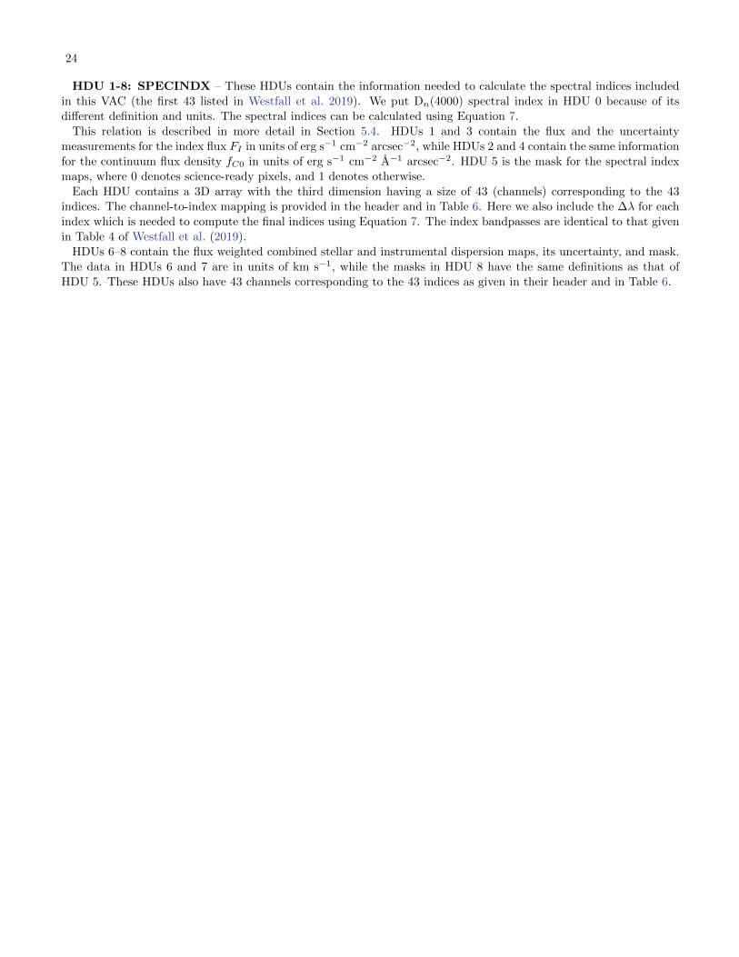
24
HDU 1-8: SPECINDX – These HDUs contain the information needed to calculate the spectral indices included
in this VAC (the first 43 listed in Westfall et al. 2019). We put Dn(4000) spectral index in HDU 0 because of its
different definition and units. The spectral indices can be calculated using Equation 7.
This relation is described in more detail in Section 5.4. HDUs 1 and 3 contain the flux and the uncertainty
measurements for the index flux FI in units of erg s−1 cm−2 arcsec−2, while HDUs 2 and 4 contain the same information
for the continuum flux density fC0 in units of erg s−1 cm−2 A−1 arcsec−2. HDU 5 is the mask for the spectral index
maps, where 0 denotes science-ready pixels, and 1 denotes otherwise.
Each HDU contains a 3D array with the third dimension having a size of 43 (channels) corresponding to the 43
indices. The channel-to-index mapping is provided in the header and in Table 6. Here we also include the ∆λ for each
index which is needed to compute the final indices using Equation 7. The index bandpasses are identical to that given
in Table 4 of Westfall et al. (2019).
HDUs 6–8 contain the flux weighted combined stellar and instrumental dispersion maps, its uncertainty, and mask.
The data in HDUs 6 and 7 are in units of km s−1, while the masks in HDU 8 have the same definitions as that of
HDU 5. These HDUs also have 43 channels corresponding to the 43 indices as given in their header and in Table 6.
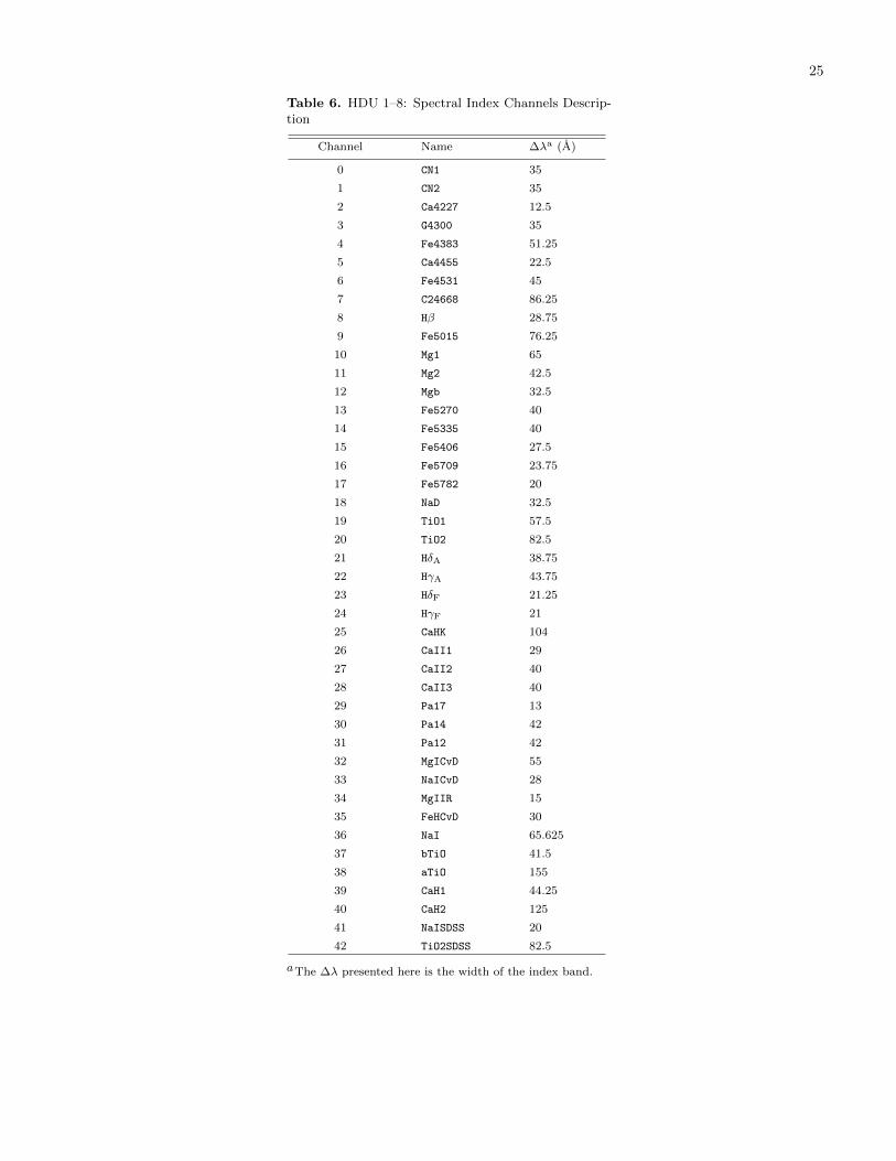
25
Table 6. HDU 1–8: Spectral Index Channels Descrip-tion
Channel Name ∆λa (A)
0 CN1 35
1 CN2 35
2 Ca4227 12.5
3 G4300 35
4 Fe4383 51.25
5 Ca4455 22.5
6 Fe4531 45
7 C24668 86.25
8 Hβ 28.75
9 Fe5015 76.25
10 Mg1 65
11 Mg2 42.5
12 Mgb 32.5
13 Fe5270 40
14 Fe5335 40
15 Fe5406 27.5
16 Fe5709 23.75
17 Fe5782 20
18 NaD 32.5
19 TiO1 57.5
20 TiO2 82.5
21 HδA 38.75
22 HγA 43.75
23 HδF 21.25
24 HγF 21
25 CaHK 104
26 CaII1 29
27 CaII2 40
28 CaII3 40
29 Pa17 13
30 Pa14 42
31 Pa12 42
32 MgICvD 55
33 NaICvD 28
34 MgIIR 15
35 FeHCvD 30
36 NaI 65.625
37 bTiO 41.5
38 aTiO 155
39 CaH1 44.25
40 CaH2 125
41 NaISDSS 20
42 TiO2SDSS 82.5
aThe ∆λ presented here is the width of the index band.

26
HDU 9–14: ELINE FLUX and ELINE EW – These HDUs contain the emission line flux maps and EW maps,
and their associated uncertainties. The emission line fluxes come from the Gaussian-fitted measurements from the
MPL-7 DAP. Again each HDU contains a 3D array with the third dimension corresponding to different emission line
channels. The channel-to-line mapping can be found in the header and in Table 7.
HDUs 9 and 10 contain the measured flux and uncertainty in units of 10−17 erg s−1 cm−2 arcsec−2, while HDUs 12
and 13 contain the EW information in units of A. HDUs 11 and 14 contain the masks for flux and EW, respectively,
defined so that 0 denotes science-ready pixels and 1 denotes otherwise.
Table 7. HDU 9–14: Emission Line Channels Descrip-tion
Channel Ion λrest (A)a
0 [O II] 3727.092
1 [O II] 3729.875
2 Hθ 3798.9826
3 Hη 3836.4790
4 [Ne III] 3869.86
5 Hζ 3890.1576
6 [Ne III] 3968.59
7 Hε 3971.2020
8 Hδ 4102.8991
9 Hγ 4341.691
10 [He II] 4687.015
11 Hβ 4862.691
12 [O III] 4960.295
13 [O III] 5008.240
14 [He I] 5877.243
15 [O I] 6302.046
16 [O I] 6365.535
17 [N II] 6549.86
18 Hα 6564.632
19 [N II] 6585.271
20 [S II] 6718.294
21 [S II] 6732.674
aVacuum rest wavelengths from the National Institute ofStandards and Technology (NIST) and are used by theMaNGA DAP.

27
HDU 15 –16: SWIFT/SDSS – HDU15 contains the sky-subtracted NUV images from Swift and optical im-
ages from SDSS, and HDU16 contains their corresponding uncertainty images. All images are provided in units of
nanomaggies. To convert these maps to the AB magnitude (m) system, use m = 22.5 − 2.5 log10(f/nanomaggie). To
convert to µJy use 1 nanomaggie = 3.631 µJy.
For 5 out of the 150 galaxies, there are bad pixels that report incorrect exposure times (usually 0 or NaN) within
the map’s FoV. In this file, the values are stored as −inf or NaN, which will cause errors in photometric measurements
if not masked. We provide masks for all Swift images in HDU 17. We strongly recommend users always use the masks
from HDU 17 when working with Swift images. If there are no bad pixels, then the mask will not change the image.
For SDSS, masked pixels have an uncertainty of 0.
In these two HDUs, the data are also given in 3D arrays with the third dimension corresponding to different filters.
The correspondence are given in the header and in Table 8.
Table 8. HDU 15–16: Photometry ChannelDescription
Channel Name Central Wavelength (A)
0 uvw2 1928
1 uvw1 2600
2 uvm2 2246
3 SDSS u 3543
4 SDSS g 4770
5 SDSS r 6231
6 SDSS i 7625
7 SDSS z 9134

28
HDU 17: SWIFT UVOT – This HDU contains the Swift/UVOT counts, uncertainty, exposure and mask maps
for all three NUV filters. The masks have a value of 0 for science-ready pixels and 1 otherwise. Unlike HDU 15 and
16, these images are not sky-subtracted. However the calculated sky counts are provided in the header under the
keywords SKY W1, SKY M2 and SKY W2. The AB magnitude system zero points of the filters and fλ conversion factors
are also provided in the header as ABZP ∗ and FLAMBDA ∗, where the ∗ represents the desired filter. The structure of
this HDU is given in Table 9.
Table 9. HDU 17: Swift/UVOT Channel Description
Channel Name Description
0 uvw2 Counts Fully reduced, non-sky subtracted uvw2 counts
1 uvw1 Counts Fully reduced, non-sky subtracted uvw1 counts
2 uvm2 Counts Fully reduced, non-sky subtracted uvm2 counts
3 uvw2 Counts Err Uncertainty associated with uvw2 counts
4 uvw1 Counts Err Uncertainty associated with uvw1 counts
5 uvm2 Counts Err Uncertainty associated with uvm2 counts
6 uvw2 Exposure Exposure map for uvw2 image
7 uvw1 Exposure Exposure map for uvw1 image
8 uvm2 Exposure Exposure map for uvm2 image
9 uvw2 Mask Mask for uvw2 image
10 uvw1 Mask Mask for uvw1 image
11 uvm2 Mask Mask for uvm2 image

29
REFERENCES
Aguado, D. S., Ahumada, R., Almeida, A., et al. 2019,
ApJS, 240, 23
Astropy Collaboration, Price-Whelan, A. M., Sipocz, B. M.,
et al. 2018, AJ, 156, 123
Baldwin, J. A., Phillips, M. M., & Terlevich, R. 1981,
PASP, 93, 5
Battisti, A. J., Calzetti, D., & Chary, R.-R. 2016, ApJ, 818,
13
Battisti, A. J., Calzetti, D., & Chary, R. R. 2017, ApJ, 851,
90
Beers, T. C., Flynn, K., & Gebhardt, K. 1990, AJ, 100, 32
Belfiore, F., Westfall, K. B., Schaefer, A., et al. 2019, AJ,
158, 160
Bentz, M. C., & Katz, S. 2015, PASP, 127, 67
Bertin, E., & Arnouts, S. 1996, A&AS, 117, 393
Blanton, M. R., Kazin, E., Muna, D., Weaver, B. A., &
Price-Whelan, A. 2011, AJ, 142, 31
Blanton, M. R., Bershady, M. A., Abolfathi, B., et al. 2017,
AJ, 154, 28
Bolton, A. S., Schlegel, D. J., Aubourg, E., et al. 2012, AJ,
144, 144
Breeveld, A. A., Curran, P. A., Hoversten, E. A., et al.
2010, MNRAS, 406, 1687
Bundy, K., Bershady, M. A., Law, D. R., et al. 2015, ApJ,
798, 7
Burrows, D. N., Hill, J. E., Nousek, J. A., et al. 2000, in
Proc. SPIE, Vol. 4140, X-Ray and Gamma-Ray
Instrumentation for Astronomy XI, ed. K. A. Flanagan &
O. H. Siegmund, 64–75
Burstein, D., Faber, S. M., Gaskell, C. M., & Krumm, N.
1984, ApJ, 287, 586
Calzetti, D. 2013, Star Formation Rate Indicators, ed.
J. Falcon-Barroso & J. H. Knapen, 419
Calzetti, D., Armus, L., Bohlin, R. C., et al. 2000, ApJ,
533, 682
Cappellari, M., & Copin, Y. 2003, MNRAS, 342, 345
Cappellari, M., & Emsellem, E. 2004, PASP, 116, 138
Charlot, S., & Fall, S. M. 2000, ApJ, 539, 718
Drory, N., MacDonald, N., Bershady, M. A., et al. 2015,
AJ, 149, 77
Evans, P. A., Beardmore, A. P., Page, K. L., et al. 2007,
A&A, 469, 379
—. 2009, MNRAS, 397, 1177
Evans, P. A., Osborne, J. P., Beardmore, A. P., et al. 2014,
The Astrophysical Journal Supplement Series, 210, 8
Fabbiano, G. 2006, Annual Review of Astronomy and
Astrophysics, 44, 323
Faber, S. M., Friel, E. D., Burstein, D., & Gaskell, C. M.
1985, ApJS, 57, 711
Garay, G., & Lizano, S. 1999, PASP, 111, 1049
Greene, J. E., & Ho, L. C. 2007, ApJ, 670, 92
Gunn, J. E., Siegmund, W. A., Mannery, E. J., et al. 2006,
AJ, 131, 2332
Hunt, L. K., & Hirashita, H. 2009, A&A, 507, 1327
Husemann, B., Jahnke, K., Sanchez, S. F., et al. 2013,
A&A, 549, A87
Kauffmann, G., Heckman, T. M., Tremonti, C., et al. 2003,
MNRAS, 346, 1055
Kennicutt, R. C., & Evans, N. J. 2012, ARA&A, 50, 531
Kennicutt, Jr., R. C. 1984, ApJ, 287, 116
—. 1998, ARA&A, 36, 189
Kewley, L. J., Groves, B., Kauffmann, G., & Heckman, T.
2006, MNRAS, 372, 961
Kim, K.-T., & Koo, B.-C. 2001, ApJ, 549, 979
Law, D. R., Cherinka, B., Yan, R., et al. 2016, AJ, 152, 83
Lehmer, B. D., Alexander, D. M., Bauer, F. E., et al. 2010,
ApJ, 724, 559
Martig, M., Bournaud, F., Teyssier, R., & Dekel, A. 2009,
ApJ, 707, 250
Martin, D. C., Fanson, J., Schiminovich, D., et al. 2005,
ApJL, 619, L1
Molina, M., Ajgaonkar, N., Yan, R., et al. 2020, MNRAS,
494, 4751
O’Donnell, J. E. 1994, ApJ, 422, 158
Osterbrock, D. E., & Ferland, G. J. 2006, Astrophysics of
gaseous nebulae and active galactic nuclei
Panessa, F., Bassani, L., Cappi, M., et al. 2006, A&A, 455,
173
Peacock, J. A. 1983, MNRAS, 202, 615
Poole, T. S., Breeveld, A. A., Page, M. J., et al. 2008,
MNRAS, 383, 627
Roming, P. W. A., Kennedy, T. E., Mason, K. O., et al.
2005, SSRv, 120, 95
Salim, S., Boquien, M., & Lee, J. C. 2018, ApJ, 859, 11
Sanchez-Blazquez, P., Peletier, R. F., Jimenez-Vicente, J.,
et al. 2006, MNRAS, 371, 703
Schlegel, D. J., Finkbeiner, D. P., & Davis, M. 1998, ApJ,
500, 525
Smee, S. A., Gunn, J. E., Uomoto, A., et al. 2013, AJ, 146,
32
Springel, V., Di Matteo, T., & Hernquist, L. 2005,
MNRAS, 361, 776
Steinhauser, D., Schindler, S., & Springel, V. 2016, A&A,
591, A51
Trager, S. C., Worthey, G., Faber, S. M., Burstein, D., &
Gonzalez, J. J. 1998, The Astrophysical Journal
Supplement Series, 116, 1

30
Wake, D. A., Bundy, K., Diamond-Stanic, A. M., et al.
2017, AJ, 154, 86
Westfall, K. B., Cappellari, M., Bershady, M. A., et al.
2019, arXiv e-prints, arXiv:1901.00856
Wild, V., Charlot, S., Brinchmann, J., et al. 2011, MNRAS,
417, 1760
Xiao, T., Wang, T., Wang, H., et al. 2012, MNRAS, 421,
486
Yan, R., Bundy, K., Law, D. R., et al. 2016, AJ, 152, 197