University of Minnesota

Department of Economics

Revised November 2017

Sweat Equity in U.S. Private Business∗

Anmol Bhandari

University of Minnesota

Ellen R. McGrattan

University of Minnesota

and Federal Reserve Bank of Minneapolis

ABSTRACT

This paper uses theory disciplined by U.S. national accounts and business census data to measureprivate business sweat equity, which is the value of time to build customer bases, client lists,and other intangible assets. We estimate an aggregate sweat equity value of 0.65 times GDP,with little cross-sectional dispersion in valuations when compared to business net incomes andlarge cross-sectional dispersion in rates of return. Our estimate of sweat equity is close to theestimate of marketable fixed assets used in production by private businesses, implying a high ratioof intangible to total assets. We use the model to evaluate impacts of greater tax compliance ofprivate businesses and lower tax rates on net income of both privately-held and publicly-tradedbusinesses.

Keywords: Intangibles, business valuation

JEL classification: E13, E22, H25

∗Bhandari acknowledges support from the Heller-Hurwicz Economic Institute, and McGrattanacknowledges support from the NSF. We thank Yuki Yao, Serdar Birinci, and Kurt See for excellentresearch assistance and seminar participants at the University of Colorado for helpful comments.The views expressed herein are those of the authors and not necessarily those of the Federal ReserveBank of Minneapolis or the Federal Reserve System.

1. Introduction

Tax advantages for pass-through entities introduced in the Tax Reform Act of 1986 have led to

rapid growth in the private U.S. business sector, which now accounts for over half of yearly business

net income reported to the Internal Revenue Service (IRS).1 Despite this growth, little is known

about private businesses because taxable incomes are understated, survey data are unreliable,

and business valuations depend importantly on unmeasured time—sweat—that owners devote to

building sweat equity, namely, the value of client lists, customer bases, and other intangible assets.

In this paper, we first provide evidence that existing measures of business incomes and valuations

are mismeasured and then develop a theory disciplined by U.S. national accounts and business

census data to measure net incomes and sweat equity in U.S. private business. Once measured, we

consider the impact of stricter tax compliance for private businesses, lower taxation of net incomes

of private business, and lower taxation of profits of Schedule C corporations.

We develop a theory of sweat equity with the key feature that business owners put time

into two activities: production of goods and services and accumulation of sweat capital—building

client lists, customer bases, goodwill, and so on. Sweat capital is an input of production, along

with plant, equipment, and hours. The income generated from sweat capital can be thought of as

dividends, whose present value is the sweat equity we are interested in measuring. Each period,

individuals choose to run their own business or work for a Schedule C corporation and the choice

is driven primarily by their productivity levels in each activity, their accumulated sweat capital,

and tax policy, which may be advantageous to time allocated to business. We assume plant and

equipment can be rented, and therefore, the main start-up cost is the labor input required for the

accumulation of sweat capital, which is not pledgeable. As in Aiyagari (1994), productivities are

stochastic and individuals are heterogeneous but, in our model, there are two productivity shocks,

one affecting business production and another affecting wages of employees in C corporations. If

the shocks are not perfectly correlated, individuals will switch between the two sectors. When

business owners switch, their sweat capital deteriorates with time.

Key parameters of our baseline model are chosen to ensure that model income and product

1 Pass-through entities such as S corporations and partnerships distribute all earnings to owners who, like soleproprietors, report business net incomes on their individual tax returns. See Cooper et al. (2016) and Smithet al. (2017) for details about these businesses based on administrative tax data.

1

shares are consistent with U.S. national account data, model taxable income distributions are

consistent with IRS data, and model business age profiles and hours are consistent with U.S. Census

data. For this baseline, we estimate an aggregate sweat equity value of 0.65 times GDP, which

is close to the estimate of fixed assets used by private businesses. We find little cross-sectional

dispersion in sweat-equity valuations when compared to business net incomes. This result follows

from the fact that there is a lot of switching in and out of business ownership in the United

States. Since the model matches this feature of the data, individuals in the model have similar

expectations of the present value of future dividend incomes arising from the accumulation of sweat

capital, even if their current business incomes are very different. Little dispersion in valuations and

large dispersion in incomes means that we find large differences in the implied rates of return on

sweat equity. The 5th to 95th percentile range for business owners is −50 to 100 percent returns.

The range for all individuals is slightly smaller at −40 to 60 percent since there are many with no

dividends.

Once we have measured the sweat equity for the baseline, we use the model to estimate the

impact of tax policy changes on the sweat equity valuations and other key economic aggregates. We

first consider policies ensuring greater tax compliance of private businesses, who understate their

adjusted gross incomes by roughly 50 percent according to calculations of the Bureau of Economic

Analysis (BEA). We find that enforcing tax compliance would have a significant, negative impact

on labor inputs and sweat capital in private business production. We also consider policy changes

that lower business tax rates, both on private businesses and Schedule C corporation profits. If

we lower both business tax rates by 10 percentage points, we find wages and GDP higher by 5

percent, C-corporate output higher by 6.5 percent, private business output higher by 9 percent,

and sweat equity higher by 6 percent.

Our paper is related to studies of small businesses and entrepreneurship. There are now

many quantitative theories of entrepreneurship. Most of them model entrepreneurs as agents

employing physical capital subject to uninsurable idiosyncratic risk and financing constraints. See,

for example, Angeletos and Calvet (2006) for a model with uninsurable capital income risk and

Buera (2009), Cagetti and DeNardi (2006), Dyrda and Pugsley (2017), Li (2002), Meh (2005),

and Quadrini (1999,2000) for analyses of models with both uninsurable capital income risks and

2

financing frictions that restrict external equity and assume collateral constraints on debt. These

studies mainly focus on the role of financial frictions in accounting for dispersion in survey-based

measures of wealth and income.2 Also related are Hurst and Pugsley (2011, 2017), who model

entrepreneurial choices as driven by non-pecuniary benefits of owning a business and use their

theory to account for survey-based differences in business incomes and wages. None of these

studies explicitly model the accumulation of the business owners sweat in building the business

and, therefore, cannot be used to estimate aggregate or cross-sectional valuations of this key

business asset or the impact of changes in taxation of pass-through entities.3

Empirically, we differ from the literature in our choice of facts to use for disciplining the the-

ory. Much of the literature has used survey data on business net incomes and valuations from

either the Federal Reserve’s Survey of Consumer Finances (SCF), the Kauffman Foundation Firm

Survey (KFS), or the Census Survey of Income and Program Participation (SIPP).4 We document

large differences between survey responses about taxable business incomes and the actual business

incomes reported on tax forms. Furthermore, the errors are not systematically biased. In the

SCF, most respondents overstate business incomes. In the SIPP, most respondents understate

business incomes. In the KFS, respondents overstate both revenues and expenses and understate

net incomes. The percentage errors vary widely over time and in the cross-section. These report-

ing errors cast serious doubt on the accuracy of self-reported assessments of business valuations,

especially for businesses with significant sweat equity.

2. Data

In this section, we motivate our interest in accounting for the sweat equity of private businesses

and describe data that can be used to guide our theory and measurement. We start with statistics

from Pratt’s Stats on business transactions and show that intangible assets—both identifiable assets

2 The literature on factor misallocation use similar theories of entrepreneurs to quantify cross-country differencesin aggregate productivity. See, for example, Buera and Shin (2013), Midrigan and Xu (2014), and Restucciaand Rogerson (2008), and Hopenhayn’s (2014) survey for a complete list of references.

3 In other literatures, researchers model investments in intangible capital—including brand and customer capital—to study trade patterns, asset pricing, firm dynamics, and business cycles, but they do not model the entryand time-use decisions of small business owners. See, for example, Arkolakis (2010), Belo, Lin, and Vitorino(2014), Drozd and Nosal (2012), Gourio and Rudanko (2014), and McGrattan and Prescott (2010).

4 See, for example, Benhabib, Bisin, and Luo (2015), Cagetti and DeNardi (2006), Hamilton (2000), Hurst andPugsley (2011), Kartashova (2014), McGrattan and Prescott (2010), Meh (2005), Moskowitz and Vissing-Jorgensen (2002), Pugsley (2011), and Quadrini (1999,2000).

3

such as customer and client lists and nonidentifiable assets such as goodwill—are a significant

fraction of the transacted values.5 While Pratt’s Stats can be used to highlight the importance

of intangible assets, this transaction dataset is not a representative sample of all business sales

and does not include information for ongoing businesses. The Federal Reserve Board’s widely-

used Survey of Consumer Finances (SCF) does have information on taxable incomes and self-

reported wealth for actively-managed businesses, but we document here that the survey responses

by proprietors, partners, and S corporation owners to questions about their business incomes are

not reliable.6 For information on business incomes, we instead use data from the IRS, and for

information on business owners, we use data from the U.S. Census Survey of Business Owners

(SBO). The SBO provides information on turnover rates of business, time allocation to business

operations, and financing requirements for business start-ups. Finally, we report relevant statistics

from the U.S. national accounts that will be matched to our model aggregates.

2.1. Business Acquisition Data

A key finding from business transactions data is that roughly 50 percent of the value is allo-

cated to assets categorized by the IRS as intangible, regardless of the business industry, age, legal

structure, or size.7 These intangible assets include customer- and information-based intangibles,

trademarks, tradenames, franchises, contracts, patents, copyrights, formulae, processes, designs,

patterns, non-compete agreements, licenses, permits, and goodwill. In Table 1, we report ratios of

intangible asset values to the total assets for a sample of 6,855 sales of businesses over the period

1994 and 2017.

We restrict attention to U.S. private businesses in three legal organization categories, namely,

S corporations, sole proprietorships, and partnerships, and we report the ratios by industry, age,

and different measures of business size.8 The ratio of intangible asset value to total asset value

5 Pratt’s Stats is a database with complete financial data on over 27,000 acquired private companies.6 We include the survey in our discussion because it is the most widely-used survey for the study of business

income and wealth. We also compare survey responses of the Kauffman Firm Survey and the SIPP to IRSdata and find large differences.

7 Both buyers and sellers file an asset acquisition statement (Form 8594) with the IRS that specifies the allocationof the purchase price to specific assets. These forms are used to determine the purchaser’s depreciable assetsand the seller’s capital gain or loss.

8 We exclude C corporations because most are public, and we exclude LLCs because Pratt’s Stats does notprovide details on the owner’s legal status. In Bhandari and McGrattan (2017), we report the statistics forthe entire database.

4

for all transactions has a mean of 58 percent and a median of 64 percent, with remaining value

attributed to cash, trade receivables, inventories, fixed assets, and real estate. We think of these

estimates as lower bounds for ongoing concerns, in part because there could be reputational loss

with a new owner.

The estimates are almost the same across legal structure, although most of the transactions are

for S corporations. By industry, we find some variation in the intangible intensity, with agriculture,

mining, and utilities (NAICS 11–22) at the low end averaging 44 percent and information and

financial (NAICS 51–53) at the high end averaging 80 percent. By age, we find an increase in the

intangible intensity, starting at an average of 44 percent for new enterprises and plateauing at an

average of 58 percent after 15 years. Conditioning on size, we find the intangible intensity rises

with sales and assets, but falls with the number of employees. Overall, the ranges of the reported

statistics are not wide.

2.2. Household Survey Data

One disadvantage of the Pratt’s Stats sample is that it is not representative and does not

include data for continuing businesses. A widely-used representative sample for all businesses is

the SCF household survey, which is specifically designed to provide information about household

wealth, including business wealth. One possible issue with the SCF is that the business valuations

are not based on transactions but rather are self-reported and therefore unlikely to be accurate

estimates for intangible-intensive businesses. A second and more serious issue is that the business

income data—which could potentially be capitalized to provide an alternative estimate of business

wealth—are not consistent with IRS data even though the households are asked to report specific

lines off of their tax forms.

In Table 2, we show data for the 2007 survey (with all other years shown in Bhandari and

McGrattan (2017)) from the SCF, which is directly comparable to the 2006 tax year data from the

IRS.9 For the individual taxes, we compare incomes for sole proprietors who file Schedule C with

their individual tax form (1040) and partners and S-corporation shareholders who file Schedule E

9 See also Johnson and Moore (2011), who compare the 2001 SCF and 2000 IRS tax year data and find largedifferences.

5

with their individual tax form. Since the SCF asks about all Schedule E income, we include income

to estates, trusts, rents and royalties along with income to partners and S-corporation shareholders.

The first three columns of Table 2 show results for sole proprietors and the second three for

partners and S corporation shareholders. The first row reports total income in billions for all

returns and the rows below have data for subgroups of tax filers who are ranked by their adjusted

gross income (AGI). The total Schedule C income earned by sole proprietors reported to the IRS in

2006 was 282 billion. The total Schedule E income earned by partners, S-corporation shareholders

and others who reported supplemental income to the IRS in 2006 was 466 billion. Aggregated

responses in the SCF were too high by more than 70 percent.10 If we consider subgroups of the

population, the errors are also large, in some cases negative and in other cases positive. The first

subgroup is the bottom half of returns filed, those with the lowest AGI. According to the SCF,

sole proprietors in this group earned 31 billion in business income (listed on their Schedule C).

The actual tax forms show 50 billion and therefore we list a −39 percent error. According to the

SCF, this same group reported 19 billion in Schedule E income when the actual income on the tax

forms was a loss of 41 billion. For the next three groups of filers, incomes reported on the SCF

are overstated relative to the actual IRS incomes and the errors are greater than 50 percent in all

cases.

The last three columns of Table 2 compares net incomes of S corporations who file Form 1120S

in addition to reporting pass-through distributions on their individual tax forms. In this case, we

sort shareholders (as opposed to returns) according to their business receipts and group the bottom

half into the first group (0 to 50) and so on. We then report their net incomes on ordinary business.

For 2006, S corporations reported 296 billion in net income to the IRS. According to the SCF,

the total was 577 billion, 95 percent too high. For the subgroups of shareholders, the incomes are

overstated for the first three subgroups—with errors greater than 100 percent—and understated

for the businesses with the highest receipts.

When we analyze the data over time, we find many incidents of errors greater than 100 percent.

10 In Bhandari and McGrattan (2017), we report comparable results for sole proprietors in the SIPP dataset fortax year 2006. In contrast to SCF households, SIPP households significantly understate net incomes. Theerror for all returns is −56 percent and between −41 and −87 percent for the same AGI subgroups that arereported in Table 2.

6

In Figure 1, we report errors for all returns for tax years 1988 to 2012. There are three estimates

per year corresponding to the three incomes reported in Table 2. For example, in tax year 2006,

the errors for Schedule C filers, Schedule E filers, and S corporations are 78, 73, and 95 percent,

respectively. In some years, the errors exceed 200 percent and show no sign of trending downward.

Even in 2012, the year with the best results, the errors are 30, 55, and 11 percent, respectively. One

reason for the discrepancies between SCF and IRS data is the fact that few respondents refer to tax

documents when answering the questionnaire. When the SCF reviewer is asked if the respondents

referred to tax documents, an average of 4 percent of households answered that they frequently

did in years prior to 2003 and 7 percent did in years after 2003. In most years, an additional

7 or 8 percent answered that they sometimes referred to tax documents. A second reason for

large discrepancies in the case of private businesses is the SCF sample size, which is too small to

generate a representative sample. For example, in the case of statistics reported in Table 2 for S

corporations, the IRS reports data for 3.9 million businesses while the SCF coverage is only 2.8

million.

In Table 3, we summarize findings of Gurley-Calvez et al. (2016), who compared responses

about receipts, expenses, and profits for businesses in the Kauffman Firm Survey with matched

tax forms. They find that the firms in the survey overstate receipts and overstate expenses by

more, leading to understated profits across the distribution. These findings are for the most part

in contrast to the SCF versus IRS comparison, which shows that most firms overstate net income.

2.3. Business Census Data

Another representative survey that we analyze is the U.S. Census survey of business owners.

The Census data do not include business valuations but do include information about businesses

and owners that, along with theory, can be used to infer sweat equity valuations. More specifically,

to discipline our model, we use information from the 2007 SBO public use microdata sample

(PUMS) on the year of the business acquisition, the hours spent working in the business, and

capital sources and requirements for business start-ups.

In Figure 2, we show the percentage of owners by years since acquiring their business. Two

profiles are plotted: one for all owners reporting and another for owners for which the business

7

is their primary source of income.11 Roughly 11 percent of business owners had just acquired

the business at the time of the survey. Conditioning on the business being the primary source of

income, 9 percent of owners had just acquired. The rate of ownership falls to about 5 percent for

businesses acquired 5 years ago and 1 percent for businesses acquired 30 years ago.

Using the Census SBO survey, we estimate average weekly hours for all owners and for owners

who report that the business income is their primary source of income. There are 37 million owners

in businesses with up to four owners working on average 33 hours per week. Of these, there are

18.3 million reporting that their primary income comes from the business, and these owners report

44 hours per week on average.12 Assuming the available stock of workers aged 16 to 64 in 2007 is

197 million and weekly discretionary time is 100 hours, the aggregate time that private business

owners devote to their business is roughly 6.2 percent of total available time (that is, 33/100×

37/197), with owners that receive primary income from the business contributing 4.1 percent of

total available time (that is, 44/100×18.3/197).13 The remaining labor input is allocated to work

in C corporations and the government, which is equal to roughly 18 and 4 percent of total time,

respectively.

The SBO also provides information on financing needs of private business owners, most of

whom are sole proprietors or S corporations and partnerships with 1 or 2 owners. Of those busi-

nesses reporting a source of start-up capital in the 2007 PUMS sample, only 12 percent had a bank

or government loan or guaranty and most of these owners borrowed a relatively small amount (less

than $100,000) when compared to average assets in private businesses. Twenty-three percent re-

ported that they needed no start-up capital. For the remaining owners, the main source of capital

was personal savings or loans from family members, with roughly 65 percent reporting this as a

source of capital. Eleven percent used credit cards and 6 percent used home equity lines.

11 The microdata sample includes information for up to four owners of the business. Only 3 percent of the 26.4million firms have more than 4 owners.

12 The number of owners reporting that the business is their primary income in the SBO is similar to the estimateof 17.2 million that comes from summing 10.4 million proprietors and partners working primarily in businessreported by the BEA and the 6.8 million S-corporation shareholders reported by the IRS.

13 For with 2 percent of businesses with more than four owners, we have only included hours of the first fourowners.

8

2.4. National Account Data

Finally, we summarize the national account data that should be consistent with aggregate

data from our theory. (See Bhandari and McGrattan (2017) for full details.) In Table 4, we report

categories of income and product in such a way as to be directly comparable to theoretical values

in the next section. The values in the right column are shares relative to total adjusted income

or product. Three adjustments are made to both totals: we subtract sales taxes, add consumer

durable depreciation and imputed services, and add additional intellectual property products (IPP)

investment categories not currently included in NIPA.14

Starting with incomes, roughly three-fourth of total adjusted income is categorized as business

income and one-fourth as non-business income to household or government. We split business

income into three categories: income to pass-through entities (sole proprietorships, partnerships,

and Schedule S corporations), labor income of workers in Schedule C corporations, and capital

income. The first category includes NIPA proprietors’ income (excluding inventory and capital

consumption adjustments, which are included with capital income). This income category includes

income to sole proprietorships and partnerships, net income to S corporations and S-corporation

compensation that is deducted from net income on Form 1120S.15 The next category of income

in Table 4 is C-corporation compensation, which is total compensation less S-corporation and

non-business compensation. Capital income is the third category of business income and includes

C-corporation profits, rental incomes, net interest, indirect business taxes less sales taxes, an

imputation for IPP investment, and depreciation. Currently, the NIPA IPP investment category

is 4 percent of NIPA GDP, which is roughly one-third of current estimates of total intangible

investments. (See Corrado et al. (2005).) The final income category includes all non-business

incomes. Non-business incomes include compensation to household, nonprofit, and government

employees, net interest and rental incomes paid to households, nonprofits, and government, indirect

business taxes paid by households and nonprofits, profits of government enterprises, imputed capital

services to consumer durables and government investment, and depreciation of residential and

government fixed assets.

14 For example, advertising and marketing costs would be included here.15 The BEA includes a large imputation for underreported income of proprietors based on estimates from tax

compliance studies. Later, we treat the NIPA data as total income and assume that businesses effectively facea lower tax rate on their income.

9

The remainder of Table 4 categories are NIPA products. Private consumption includes con-

sumption of nondurables and services less sales taxes and imputations for capital services and

durable depreciation. Government consumption is the same as in NIPA. Investment is divided into

business and non-business as in the case of incomes. We split business investments into that of C

corporations and that of pass-through entities using data from the BEA fixed asset tables and IRS

corporate filings. Nonbusiness investments include consumer durables less sales tax, residential

and government investment, and net exports.

Next, we develop a theory consistent with the facts laid out above.

3. A Theory of Sweat Equity

In the model economy that we analyze, households can choose to work for large public firms

(C corporations) or small private firms (S corporations, sole proprietorships, and partnerships).16

There are two key features in our model that distinguish public and private firms. The first

is taxation: C corporations pay corporate income tax while most private firms are small, pass-

through entities that avoid taxation of profits. A second distinction is the underlying assets of the

business. In the case of small private businesses, a large component of their value is accumulated

sweat (time) to build the business customer base, client list, and other business intangibles. This

time is not compensated with wage payments but rather as capital gains.17

At a point in time, the state vector for households includes financial assets a, sweat capital κ,

productivity in C-corporate work ǫ, and productivity in running one’s own business z. Households

choose to allocate their time to C-corporate work or running a business to maximize the overall

value:

V (a, κ, ǫ, z) = max{Vc (a, κ, ǫ, z) , Vs (a, κ, ǫ, z)}.

where Vc(·) is the value to working in the C corporation and Vs(·) is the value to running one’s

own business (whether it be an S corporation, a sole proprietorship, or a partnership).

16 In reality, some C corporations are small and some are privately-held. However, most C corporations are large,publicly-traded companies, and most S corporations, sole proprietors, and partnerships are small, privately-heldcompanies.

17 Much of C-corporation intangible investment does show up in the national accounts as intermediate purchasesor employee compensation. A good example of the latter is wage compensation to R&D scientists.

10

The problem of working in a C corporation is relatively standard. In this case, the households

choose consumption of goods produced by the large firms, cc, consumption of goods produced by

the small private firms, cs, leisure ℓ, and financial assets next period a′ to maximize the value

function:

Vc (a, κ, ǫ, z) = maxcc,cs,ℓ,a′

{U (cc, cs, ℓ) + β∑

ǫ′,z′

π (ǫ′, z′|ǫ, z) V (a′, κ′, ǫ′, z′)} (3.1)

subject to

a′ = [(1 + r)a + wǫn − (1 + τc) (cc + pcs)

− Tw (wǫn) + ynb − xnb]/ (1 + γ)

κ′ = λκ

ℓ = 1 − n

a ≥ 0,

where r is the after-tax interest rate on financial assets, w is the wage rate, p is the relative

price of goods produced by small private firms, τc is the tax levied on consumption, Tw(·) is the

tax function on labor earnings, ynb is (exogenous) nonbusiness income, and xnb is (exogenous)

nonbusiness investment. Technology grows at rate γ and all variables are assumed to be divided

by (1 + γ)t. We also assume that any sweat capital accumulated in past businesses deteriorates at

rate λ, which could be immediately and then κ′ = 0.

If households instead choose to run a business, then in addition to consumptions, leisure,

and financial assets, they choose how to allocate working time between growing the business and

production. They also need to decide how much plant and equipment to rent.18 The maximization

problem in this case is:

Vs (a, κ, ǫ, z) = maxcc,cs,a′,hy,hκ,ks

{U (cc, cs, ℓ) + β∑

ǫ′,z′

π (ǫ′, z′|ǫ, z) V (a′, κ′, ǫ′, z′)} (3.2)

subject to

a′ = [(1 + r) a + pys − (r + δk) ks − x − (1 + τc) (cc + pcs)

18 Here, we assume that they rent marketable fixed assets such as physical plant and equipment. We would getthe same results if they owned the capital, since their financial assets are claims to earnings from marketablefixed assets.

11

− T b (pys − (r + δk) ks − x) + ynb − xnb]/ (1 + γ)

κ′ = [(1 − δκ) κ + fκ (x, hκ)] / (1 + γ)

ys = zfy (κ, ks, hy)

ℓ = 1 − hκ − hy

a′ ≥ max (0, χpys) ,

where the hours allocation is hκ to growing the business and hy to production and the marketable

fixed assets is ks which is rented at rate r. The business income is sales pys less rental payments

(r + δk)ks and any expenses used in producing new sweat capital x.19 The constraint on assets for

the business owners now depends on the term χpys, which can be interpreted as a working capital

constraint for business owners.20

C-corporations choose hours nc and fixed assets kc to solve

maxkc,nc

yc − wnc − (rk + δk) kc

subject to yc = AF (kc, nc). Here, rk is the before-tax rental rate on capital.

The government spends g, borrows b and collects taxes on consumption, labor earnings, private

business income, C-corporation dividends, and C-corporation profits. The government budget

constraint is given by:

g + (r − γ) b = τc

(∫

ccidi +

∫

pcsidi

)

+

∫

Tw (wǫini) di

+

∫

T b (pysi − (r + δk) ksi − xi) di + τp (yc − wnc − δkkc)

+ τd (yc − wnc − (γ + δk) kc − τp (yc − wnc − δkkc)) . (3.3)

Here again we assume that all variables are divided by the technological trend growth.

19 The sales should be interpreted as net of any outside labor services, which we include later with C corporationproduction. The model can be extended to include a fourth factor of production, namely, employees that arenot owners or shareholders in the business.

20 Motivated by the work of Hurst and Lusardi (2004) and evidence about financing needs from the SBO, we setχ = 0 in our baseline model and then check the sensitivity of our results to this choice.

12

In equilibrium, rental and wage rates are equated to marginal products

rk = AFk (kc, nc) − δk

w = AFn (kc, nc)

and, since private firms are for the most part pass-through entities that do not pay corporate

profits, it must be the case that

r = (1 − τp) rk

Market clearing implies that:

yc =

∫

cci di +

∫

xi di + (γ + δk)

(

kc +

∫

ksi di

)

+ g

nc =

∫

niǫi di

∫

ai di = b + (1 − τd) kc +

∫

ksi di

∫

ysi di =

∫

csi di,

where 1 − τd is the price of C-corporate fixed assets and (1 − τd)kc is the value of this capital.

Once we compute an equilibrium for the model economy, we can compute the variable of

interest, namely the value of sweat equity Vb:

Vb (a, κ, ǫ, z) = d + β∑

ǫ′,z′

π (ǫ′, z′|ǫ, z) U (c′c, c′

s, ℓ′) Vb (a′, κ′, ǫ′, z′) /U (cc, cs, ℓ)

where d is the sweat dividend is the payment to the business owner for putting time into accumu-

lating intangible investments like client lists. This dividend is equal to φpys −x. Note that a value

can be computed for all individuals, including those working in C corporations.

Given a value for sweat equity, we can compute the intangible intensity of business i by

computing the ratio

Ii =Vbi (ai, κi, ǫi, zi)

Vbi (ai, κi, ǫi, zi) + ksi,

which is comparable to the Pratt’s Stats estimates discussed earlier.

13

4. Model Parameters

In this section, we choose parameters to ensure that key statistics of the model are consistent

with data from the U.S. census of businesses, the IRS, and the U.S. national accounts. Specifically,

we choose parameters of preferences, technologies, and stochastic processes to match data on busi-

ness acquisitions, time devoted to business, financing requirements, dispersion in taxable incomes,

and the national accounts.

We start with our functional form choices for the utility function U(·), the production tech-

nology F (·) of C corporations, and the production technologies fy(·) and fκ(·) available to private

businesses, namely,

U (cc, cs, ℓ) =(

c (cc, cs)ηℓ1−η

)1−µ/ (1 − µ)

c (cc, cs) = (ωcρc + (1 − ω) cρ

s)1/ρ

F (kc, nc) = kθcn1−θ

c

fy (κ, ks, hy) = κφkαs hν

y

fκ (x, hκ) = xϑhεκ

where φ+α+ν = 1 and ϑ+ε < 1. In addition to the parameters of these functions, we need to set

depreciation rates δk, δκ, the discount rate β, the growth rate γ, the rate of deterioration of sweat

capital λ, nonbusiness shares xnb/y and ynb/y, and all fiscal variables in (3.3). The level of TFP

in C-corporate production, which is given by A, is set so that yc is normalized to 1 in equilibrium.

The first step is to choose parameters that ensure the model’s national accounts are consistent

with Table 4 and the data on time allocation in business and nonbusiness. The model accounts,

which can be matched directly to the table, are as follows:

Incomes:

Pass-through entities (sweat) (p∫

ysi di − (r + δk)∫

ksi di −∫

xi di)/y

C-corporation labor income wnc/y

Capital income ((rk + δk)kc + (r + δk)∫

ksi di)/y

Non-business income ynb/y

Products:

Private consumption (∫

cci + pcsi) di)/y

14

Government consumption g/y

C-corporation investment xc/y

Pass-through investment∫

xsi di/y

Non-business investment xnb/y

where xc and {xsi} are investments in fixed assets used in the C corporations and private businesses,

respectively.

To achieve a close match to the NIPA C corporation labor income shares, we set θ = 0.41.

To match the sweat income and time allocated to the business, we set φ = 0.15, ν = 0.45, and

residually α = 0.4. To match an overall allocation of time to work in business of 24 percent, we

set η = 0.42. Since output in C corporations is normalized and ynb is set exogenously, we can vary

ω to match the relative size of pass-through output to total output. With an estimate for total

output y, we use estimates from Table 4 and set xnb = 0.185, ynb = 0.451, and g = 0.234. To pin

down the depreciation on non-sweat capital (that is, kc and∫

ksi di), we used NIPA fixed asset

tables and set δk = 0.05. For growth of technology, we use γ = 0.02 and to match a 4 percent

annual interest rate, we set β = 0.98. For curvature in preferences, we use a standard estimate of

µ = 1.5.

For tax rates, we use effective rates based on NIPA government revenues and IRS data. The

tax rate on consumption is τc = 0.06, which is based on NIPA sales tax data. The effective tax on

dividends is τd = 0.14 and is found by multiplying the marginal rate from taxable distributions and

the fraction of distributions that are taxable. The tax rate on C-corporation profits is τp = 0.33,

which is total tax revenues divided by profits. In our baseline computations, we assume that the

tax functions Tw(·) and T b(·) are proportional, with rates τw and τb. The tax rate on labor income

from C corporations is τw = 0.4 and includes federal, state, local, and payroll taxes. The effective

tax rate on the sweat income of pass-through entities τb is assumed to be 0.2 or one-half of τw,

since the rate of underreporting found by tax compliance studies used by the BEA when imputing

proprietors income is roughly 50 percent.21 Net borrowing in the baseline is 1.2 percent of output,

which pins down the stock of debt and then transfers residually.

21 See Ledbetter (2007). Note that S corporations also have an incentive to report wage income as a distributionto avoid payroll taxes.

15

Stochastic processes for productivity are chosen to match dispersion in C-corporation wages

and pass-through incomes (with means of ǫ and z both normalized to 1.) We consider two baseline

cases. The first is uncorrelated autoregressive processes for the logarithm of z and e—both with a

serial correlation of 0.7 and standard deviation of 0.01—mapped to a 25-state Markov chain. The

second uses the same transition matrix, but we replace the values of z with values of z2 in order

to generate more skewness in sweat incomes.

The rate of switching between working as an employee and running a business depends primar-

ily on our choices of the productivity processes, the share of sweat capital in production (φ), and

the deterioration of sweat capital for C-corporate workers (λ). With the productivity parameters

and φ already chosen to match other moments, we set λ = 0.5 so as to generate a reasonable match

to the acquisition profile in Figure 2.

We do not have independent information on the remaining parameters, namely, the deprecia-

tion rate on sweat capital, δκ, and the production parameters for new sweat capital, ε and ϑ. For

the depreciation rate, we use the same rate as other capital, namely, δκ = 0.05, in our baseline

computations. For production of sweat, we assume some diminishing returns and set ε = ϑ = 0.4.

In all cases, we run sensitivity tests.

In Table 5, we report our model’s national accounts for the case that ln z is normally distributed

and the case with the z process more skewed (and all other parameters the same). In the first case,

the equilibrium wage rate w is 3.093, the price of cs goods is 1.140, and the pre-tax return rk is

0.06384. In the second case, with z more skewed, the equilibrium wage rate is 3.133, the price of

cs goods is 0.9985, and the pre-tax return is 0.06376. We see that the model does well in matching

the aggregate data for for both productivity processes.

In Figure 3, we plot our model’s prediction for the acquisition profile, for both the normal

productivity and the skewed productivity cases, along with the profile for business owners in the

SBO. The model profiles bracket the data, with greater skewness in productivity leading to more

switching between work and running a business and hence a steeper profile.

In Figure 4, we plot Lorenz curves for IRS taxable incomes along with our model’s predictions

in the baseline case with skewed productivity shocks. Figure 4A shows IRS wages, which we

16

match up to our model’s C-corporate wages. Figure 4B shows IRS business incomes on Form 1040

Schedules C and E (for sole proprietors, partners, and S corporations), along with our model’s

business income. Despite the fact that we have only 25 states in the Markov chain governing

productivity shocks (ǫ, z), we do well in matching the overall dispersion in taxable incomes, with

the exception of business incomes in the highest percentiles of the population that are more skewed

in the data than in the model.22

5. Results

In this section, we use the model for two purposes. First, we use it to measure the aggregate

value of sweat equity, its distribution, and the dispersion in the associated rates of return. Second,

we use the model to quantify the impact of changing business taxation.

5.1. Valuations and Returns

We start with our main aggregate estimates of the total value of sweat equity∫

Vbi di, ag-

gregating across all individuals, and the intangible intensity∫

Ii di, aggregating across all private

businesses and then discuss the distributions.

In the model with normally distributed business productivity shocks, we find that the aggre-

gate value of sweat equity is equal to 0.63 times GDP. In the case of skewed productivity shocks,

we find that the aggregate value of sweat equity is 0.65 times GDP. The intangible intensities for

private businesses in the two baseline cases are given by 0.44 in the case that ln z is normally

distributed and 0.51 in the case that it is skewed. In other words, sweat equity is large and roughly

as valuable for businesses as fixed assets.

In Table 6, we report our findings for the cross-sectional distributions in the baseline case with

skewed productivity shocks.23 The first column reports cross-sectional statistics for the intangible

intensity of private businesses. Recall that this is the ratio of the sweat equity Vb to the value of

sweat equity and fixed assets ks used in production. The average intensity is 51 percent, with a

22 We have made an extreme assumption in the model that individuals work in one sector or another. Relaxingthis assumption would imply a better fit of the model, but would make the model less tractable.

23 See Bhandari and McGrattan (2017) for all results shown here and below in the case with normally distributedproductivity shocks.

17

standard deviation of 29 percent, and the median is slightly higher at 53 percent. Looking across

the distribution, we find intensities of 20 percent at the 10th percentile and 97 percent at the 90th

percentile.

In the next column of Table 6, we report the sweat equity values, all relative to the median,

and find little dispersion in these values. The sweat equity value at the 10th percentile is 0.71

times the median and the sweat equity value at the 90th percentile is 1.50 times the median. Little

dispersion in sweat equity values follows from the fact that there is significant switching in and

out of business ownership. The value of a business is the present value of future dividend incomes,

which is not that different for owners facing the same stochastic process for productivity, even if

their current incomes are significantly different. This reasoning is also consistent with the fact that

there is substantial dispersion in intangible intensities and little dispersion in sweat equity values.

The greater dispersion in intangible intensities reflects the fact that current incomes and therefore

production varies significantly and thus there is wide dispersion in the use of fixed assets.

Dispersion in current incomes relative to values translates into significant dispersion in rates

of return to sweat equity. In Table 6, we report both the gross return and the dividend yield in

order to compare the results to cross-sectional data for which we only have dividend yields. For

business owners, the mean gross return is 11.4 percent with a standard deviation of 23 percent.

The dividend yield is 3.5 percent and therefore the mean capital gain is 7.9 percent. The median

gross return is 9.2 with a dividend yield of 2.1. The 10th to 90th percentile range in gross returns

is −16.7 to 44.5, with most of the difference to due to capital gains.

The full histogram for sweat equity returns is displayed in Figure 5A, along with the fitted

kernel. This shows the full range of returns is about −50 percent to over 100 percent. Because of

this dispersion, the commonly-used procedure of estimating wealth as the ratio of income divided by

a common rate of return—sometimes called capitalizing income—-would lead to wrong answers.

Following such a procedure would lead to the conclusion that there is significant dispersion in

valuations.

The next set of statistics shown in Table 6 are sweat equity valuations and returns for all

individuals. Even those working for Schedule C corporations have an expected future income from

running a business and may well have accumulated some sweat capital (κ) from past investments

18

in a business. Considering all individuals instead of just business owners increases the dispersion

in the value of sweat equity Vb, but not by much. We find that the mean to median ratio is slightly

higher, at 1.17, and the sweat equity value at the 90th percentile is a little more than double that

of the 10th percentile. The mean gross return to sweat equity is 4.6 percent, with a dividend yield

of 1.4 percent and capital gain of 3.2 percent. Figure 5B shows the full histogram of the gross

returns of all individuals. The figure shows wide dispersion, although less than for current business

owners.

In Figure 6, we display the model’s Lorenz curves for sweat equity, sweat capital, and dividends

to clearly illustrate the differences in dispersion across these measures. As the figure shows, there

is far more dispersion in the income measure d than the valuation Vb, with the capital stock κ

falling somewhere between.

In Table 6, we also compare our estimates of dividend yields to the empirical analogues in the

2007 SCF. We focus on SCF dividend yields—net incomes of actively managed businesses divided

by the business net worth—since capital gains are not available. Earlier, we showed that SCF

net incomes, when aggregated, are grossly in error. Here, we show that these errors translate into

implausibly high estimated returns. The mean SCF dividend yield, which is a lower bound for the

gross return, is 307 percent with a standard deviation of 2,813. This estimate is significantly higher

than our 3.5 percent prediction and any estimate of mean U.S. corporate dividend yields (say, for

example, based on NIPA data or Standard & Poor’s company data). Even the median firm has

high yields estimated at 20 percent, again significantly higher than our 2.1 percent prediction. At

the 90th and 99th percentiles, businesses report 500 and 5,000 percent yields.24

In Table 7, we sort businesses in our skewed productivity baseline case by their gross returns

and then examine their cross-sectional characteristics. The first column shows the age in years of

the business. The average age for firms in the 4.5 to 11.9 percent range, which includes the median,

is 15.4 years. Many of the youngest firms are in the 14.7 to 19.4 percent range, which is why the

average age in this group is the lowest at 5.1 years. The difference between businesses with the

very highest and lowest returns is only 4 years.

24 We find implausibly high SCF dividend yields even when restricting the sample to high net worth businesses.For example, considering only businesses with net worth above the median, we find average yields of 33 percent.

19

The next column of Table 7 shows how the intangible intensities covary with returns. The

businesses with the lowest intensities are building up sweat equity, are relatively younger, with

above average returns. The range in intensities across brackets is 29 percent to 71 percent, well

within the range shown in Table 6.

The final columns of Table 7 show how factors of production and outputs of private businesses

covary with returns. We find much less variation in sweat capital after sorting by returns than in

fixed assets, hours, and output. The latter depend importantly on a firm’s level of productivity,

although we can see that it is not strictly monotonic, since shocks occur and drive returns higher

or lower. Sweat capital shows no pattern and ranges from 0.27 to 0.40. Fixed assets, hours, and

output are lowest for businesses with near-zero returns and highest for businesses with above-

average returns.

We turn next to use the model for analyzing tax changes that affect businesses, both private

and public

5.2. Counterfactuals

We analyze three changes in business taxation and report the impact on key statistics for the

economy. In the first case, we experiment with greater tax enforcement for private businesses,

raising the effective tax rate from 20 percent to 35 percent. In the second case, we consider a

lower tax rate on private businesses with similar tax compliance, implying a rate decrease from

20 percent to 10 percent. Finally, we consider lowering tax rates on all businesses, both private

and public: private businesses are assessed an effective 10 percent rate and C corporations are

assessed a 20 percent rate, down from 30 percent in the baseline. In all cases, we report results for

the skewed productivity baseline. (See Bhandari and McGrattan (2017) for results with normally

distributed productivity shocks.)

The main results are shown in Table 8 and are displayed as percent changes relative to the

baseline case. The first column shows the impact of having greater compliance. Recall that private

firms in the baseline report roughly half of their actual income and thus face an effective tax rate

of 20 percent, rather than the statutory 40 percent. In this counterfactual experiment, we assume

that there is greater compliance, leading to an effective 35 percent tax rate and 7.67 percent higher

20

tax revenues. As expected, this change affects private businesses more than C corporations. The C-

corporate wage falls only 0.22 percent, but the relative price p of private small business goods rises

10 percent. Consumption, and therefore production, of such goods falls 14 percent. Investment

shifts from private business, falling by roughly 6 percent, to C corporations, rising by roughly 2

percent. Because C corporations contribute most to value added in the aggregate economy, GDP

rises by only 0.6 percent. Hours in the production of new sweat capital and private business output

are most affected, both falling about 23 percent. The sweat capital stock falls 18 percent while the

stock of fixed assets used in production falls 6 percent. The C-corporate stock of fixed assets rises

2 percent and, with the interest rate higher, financial assets rise 23 percent. Despite a large drop

in the sweat capital stock, the the decline in sweat equity values is modest, at roughly 3 percent,

since Vb is a measure of the value of future business income.

In the second experiment, we lower the tax rate on private businesses to an effective rate of 10

percent, down from 20 percent in the baseline. This experiment, which is reported in the second

column of Table 8, serves as a useful benchmark when we lower all business taxes, since factors

of production can be shifted relatively easily across sectors. With only a lowering of the tax rate

on private business, tax revenues fall by 5.28 percent. As in the greater compliance case, we find

more significant changes in activity in private business than in C corporations. Consumption of

private business goods is higher by almost 9 percent, and consumption of C-corporate goods is

lower by roughly 2 percent. These changes are accomplished with a shift of hours and capital out

of C corporations and into private business. The shift out of C corporations implies a slight drop

in GDP of roughly 0.3 percent. Increased hours in the building of new sweat capital leads to a rise

of the stock by 11 percent and a rise in sweat equity of nearly 4 percent.

The final experiment involves a lowering of the tax rate on private business net income to 10

percent and, additionally, the corporate income tax rate to 20 percent, down from 30 percent in

the baseline. The results are reported In the third column of Table 8. For this case, we find that

tax revenues are lower, but by less than in the case with only a lower tax rate on private business.

Lowering the tax rate on corporate income implies a significant rise in C-corporate wages, which

are taxed at 40 percent. Consumptions and outputs are now higher in both sectors and GDP is

higher by 4.7 percent. Factors of production are all higher, most notably hours building up sweat

21

capital and producing private output, which both rise roughly 13 percent, and fixed assets used

by C corporations, which rises almost 15 percent. Despite the increases in capital stocks in both

sectors, financial assets are lower by 4.9 percent because the level of government debt needed to

balance the budget is lower.

But, with taxes lower in both sectors, future sweat dividends are even more valuable, implying

a significant rise in sweat equity, more than 6 percent. The higher sweat equity values imply less

switching between sectors and flatter profiles of business acquisitions. (See Figure 3.) This implies

fewer start-ups and longer durations for private businesses.

6. Conclusions

In this paper, we used theory and U.S. data to measure sweat equity in private business. We

find it is large—about as large as fixed assets—and varies little in the cross section. We then

showed that tax policy changes of the magnitude being discussed by U.S. policymakers would have

a significant effect on key economic aggregates and the allocation of hours and capital to production

in privately-held versus publicly-traded businesses.

22

A. Data Sources

The main sources of data reported in the main text are as follows:

• Survey of Current Finances of the Board of Governors of the Federal Reserve System.

• Statistics of Income of the Internal Revenue Service.

• Characteristics of Business Owners of the Department of the Census.

• Pratt’s Stats of Business Valuation Resources.

• National Income and Product Accounts and Fixed Assets of the Department of Commerce,

Bureau of Economic Analysis.

23

References

Aiyagari, S. Rao, 1994, “Uninsured idiosyncratic Risk and Aggregate Saving,” Quarterly Journal

of Economics, 109(3): 659-84.

Angeletos, George-Marios and Laurent-Emmanuel Calvet, 2006, “Idiosyncratic Production Risk,

Growth and the Business Cycle,” Journal of Monetary Economics, 53(6): 1095-1115.

Arkolakis, Costas, 2010, “Market Penetration Costs and the New Consumers Margin in Interna-

tional Trade,” Journal of Political Economy, 118(6): 1151–1199.

Belo, Frederico, Xiaoji Lin, and Maria Ana Vitorino, 2014, “Brand Capital and Firm Value,”

Review of Economic Dynamics, 17: 150–169.

Benhabib, Jess, Alberto Bisin, and Mi Luo, 2015, “Wealth Distribution and Social Mobility in the

US: A Quantitative Approach,” NBER Working Paper 21721.

Bhandari, Anmol and Ellen R. McGrattan, 2017, “Technical Appendix: Sweat Equity in U.S. Pri-

vate Business,” Working paper, University of Minnesota. nnals of Finance

Buera, Francisco J., 2009, “A Dynamic Model of Entrepreneurship with Borrowing Constraints:

Theory and Evidence” Annals of Finance, 5(34): 443–464.

Buera, Francisco J. and Yongseok Shin, 2013, “Financial Frictions and the Persistence of History:

A Quantitative Exploration,” Journal of Political Economy, 121(2): 221–272.

Cagetti, Marco and Mariacristina DeNardi, 2006, “Entrepreneurship, Frictions, and Wealth,” Jour-

nal of Political Economy, 114(5): 835-870.

Cooper, Michael, John McClelland, James Pearce, Richard Prisinzano, Joseph Sullivan, Danny

Yagan, Owen Zidar, Eric Zwick, 2016, “Business in the United States: Who Owns It, and How

Much Tax Do They Pay?” Tax Policy and the Economy 30, National Bureau of Economic

Research (Chicago, IL: University of Chicago Press).

Corrado, Carol, Charles R. Hulten, and Daniel E. Sichel, 2005, “Measuring Capital and Technology:

An Expanded Framework,” in C. Corrado, J. Haltiwanger, and D. Sichel (eds.), Measuring

Capital in the New Economy, 11–46 (Chicago: University of Chicago Press).

Drozd, Lukasz A. and Jaromir B. Nosal, 2012, “Understanding international prices: Customers as

capital,” American Economic Review, 102(1): 364–95.

Dyrda, Sebastian and Benjamin Pugsley, 2017 “Taxes, Regulations of Businesses, and Evolution

of Income Inequality in the US, Working paper, University of Toronto.

Gourio, Francois and Leena Rudanko, 2014, “Customer Capital,” Review of Economic Studies,

81(3): 1102–1136.

Gurley-Calvez, Tami, Donald Bruce, E.J. Reedy, and Josh Russell, 2016, “Comparing Survey

24

Data and Tax Data: Differences in Reporting Across Businesses,” Working paper, Statistics of

Income.

Hamilton, Barton H., 2000, “Does entrepreneurship pay? An empirical analysis of the returns to

self-employment,” Journal of Political Economy, 108(3):604631.

Hopenhayn, Hugo A., 2014, “Firms, Misallocation, and Aggregate Productivity: A Review,” An-

nual Review of Economics, 6(1): 735–770.

Hurst, Erik G. and Annamaria Lusardi, 2004, “Liquidity Constraints, Household Wealth, and

Entrepreneurship, Journal of Political Economy, 112, 319–47.

Hurst, Erik G., and Benjamin W. Pugsley, 2011, “What Do Small Businesses Do? Brookings Papers

on Economic Activity 43(2): 73–142.

Hurst, Erik G., and Benjamin W. Pugsley, 2017, “Wealth, Tastes, and Entrepreneurial Choice,”

in Measuring Entrepreneurial Businesses: Current Knowledge and Challenges, eds. J. Halti-

wanger, E. Hurst, J. Miranda, and A. Schoar (Chicago: University of Chicago Press).

Johnson, Barry and Kevin Moore, 2011, “Comparing the Source: Differences in Estimates of

Income and Wealth from Survey and Tax Data,” Compendium of Federal Tax and Personal

Wealth Studies, Chapter 9, Statistics of Income.

Kartashova, Katya, 2014, “Private Equity Premium Puzzle Revisited,” American Economic Re-

view, 104(10): 3297–34.

Kitao, Sagiri, 2008, “Entrepreneurship, Taxation, and Capital investment,” Review of Economic

Dynamics, 11: 44-69.

Ledbetter, Mark, 2007, “Comparison of BEA Estimates of Personal Income and IRS Estimates of

Adjusted Gross Income,” Survey of Current Business, 87(11): 35–41.

Li, Wenli, 2002, “Entrepreneurship and Government Subsidies: A General Equilibrium Analysis,”

Journal of Economic Dynamics and Control, 26: 1815–1844.

McGrattan, Ellen R. and Edward C. Prescott “Unmeasured Investment and the Puzzling U.S. Boom

in the 1990s” American Economic Journal: Macroeconomics, 2(4): 88–123, October 2010.

Meh, Cesaire, 2005, “Entrepreneurship, Wealth Inequality, and Taxation,” Review of Economic

Dynamics, 8(1): 688–719.

Midrigan, Virgiliu and Daniel Y. Xu, 2014, “Finance and Misallocation: Evidence from Plant-level

Data,” American Economic Review, 104(2): 422–458.

Moskowitz, Tobias J. and Annette Vissing-Jorgensen, 2002, “The Returns to Entrepreneurial In-

vestment: A Private Equity Premium Puzzle?” American Economic Review, 92(4): 745–78.

Quadrini, Vincenzo, 1999, “The Importance of Entrepreneurship for Wealth Concentration and

Mobility,” Review of Income and Wealth, 45(1): 1–19.

25

Quadrini, Vincenzo, 2000, “Entrepreneurship, Saving, and Social Mobility,” Review of Economic

Dynamics, 3(1): 1–40.

Restuccia, Diego and Richard Rogerson, 2008, “Policy distortions and aggregate productivity with

heterogeneous establishments” Review of Economic Dynamics, 11(4): 707–720.

Smith, Matthew, Danny Yagan, Owen Zidar, and Eric Zwick, 2017, “Capitalists in the Twenty-first

Century,” Working Paper, United States Treasury.

26

Figure 1. Percent Differences Between Aggregate SCF and SOI Estimates

27

Figure 2. Business Acquisition Profile, U.S. Census Data

Figure 3. Business Acquisition Profile, Data and Model Baselines

28

Figure 4. Taxable Incomes, Data and Model

A. Wages

B. Business Incomes

29

Figure 5. Model Returns to Sweat Equity

A. Business Owners

B. All individuals

30

Figure 6. Model Lorenz Curves, All individuals

31

Table 1. Ratios of Intangible Asset Value to the Business Total Assets

By Legal Structure, Industry, Age, and Measures of Sizea

Characteristic Count Mean Median Std. Dev.

Legal StructureS Corporations 5,519 0.58 0.64 0.32Sole Proprietors 1,140 0.57 0.64 0.31Partnerships 196 0.57 0.67 0.32

Industry (NAICS)11–22 26 0.44 0.47 0.3123–33 975 0.60 0.65 0.3442–49 1,618 0.56 0.62 0.2951–53 420 0.80 0.93 0.2754–56 1,156 0.75 0.83 0.2461–81 2,658 0.48 0.49 0.31

Age0–1 104 0.44 0.45 0.341–2 217 0.54 0.53 0.322–4 509 0.55 0.57 0.334–15 2,772 0.59 0.65 0.2815+ 2,633 0.58 0.64 0.28

Employment0–2 1,432 0.60 0.67 0.322–3 653 0.59 0.63 0.313–5 1,043 0.55 0.62 0.315–10 1,147 0.55 0.60 0.3010+ 985 0.57 0.62 0.35

Net Sales ($ thousands)0–178 1,334 0.56 0.63 0.34178–323 1,355 0.54 0.58 0.32323–560 1,385 0.57 0.62 0.31560–1,167 1,392 0.59 0.66 0.291,167+ 1,383 0.63 0.70 0.32

Total Assets ($ thousands)1–75 1,325 0.48 0.48 0.3475–143 1.358 0.54 0.56 0.32143–254 1,377 0.59 0.65 0.33254–550 1,405 0.64 0.71 0.28550+ 1,389 0.65 0.72 0.28

All Transactions 6,855 0.58 0.64 0.32

a Transactions include only sales of S corporations, sole proprietorships, and partnerships in the Pratt’s Stats

database over the period 1990–2017.

32

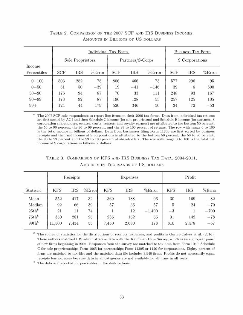
Table 2. Comparison of the 2007 SCF and IRS Business Incomes,

Amounts in Billions of US dollars

Individual Tax Form Business Tax Form

Sole Proprietors Partners/S-Corps S Corporations

Income

Percentiles SCF IRS %Error SCF IRS %Error SCF IRS %Error

0−100 503 282 78 806 466 73 577 296 95

0−50 31 50 −39 19 −41 −146 39 6 500

50−90 176 94 87 70 33 111 248 93 167

90−99 173 92 87 196 128 53 257 125 105

99+ 124 44 179 520 346 50 34 72 −53

a The 2007 SCF asks respondents to report line items on their 2006 tax forms. Data from individual tax returnsare first sorted by AGI and then Schedule C income (for sole proprietors) and Schedule E income (for partners, Scorporation shareholders, estates, trusts, renters, and royalty earners) are attributed to the bottom 50 percent,the 50 to 90 percent, the 90 to 99 percent, and the 99 to 100 percent of returns. The row with range 0 to 100is the total income in billions of dollars. Data from businesses filing Form 1120S are first sorted by businessreceipts and then net income of S corporations is attributed to the bottom 50 percent, the 50 to 90 percent,the 90 to 99 percent and the 99 to 100 percent of shareholders. The row with range 0 to 100 is the total netincome of S corporations in billions of dollars.

Table 3. Comparison of KFS and IRS Business Tax Data, 2004-2011,

Amounts in Thousands of US dollars

Receipts Expenses Profit

Statistic KFS IRS %Error KFS IRS %Error KFS IRS %Error

Mean 552 417 32 369 188 96 30 169 −82

Median 92 66 39 57 36 57 5 24 −79

25thb 21 11 74 1 12 −1,400 −3 1 −700

75thb 350 281 25 236 152 55 31 142 −78

99thb 11,500 7,434 55 7,450 2,680 178 810 2,478 −67

a The source of statistics for the distributions of receipts, expenses, and profits is Gurley-Calvez et al. (2016).

These authors matched IRS administrative data with the Kauffman Firm Survey, which is an eight-year panel

of new firms beginning in 2004. Responses from the survey are matched to tax data from Form 1040, Schedule

C for sole proprietorships Form 1065 for partnerships Form 1120S or 1120 for corporations. Eighty percent of

firms are matched to tax files and the matched data file includes 3,940 firms. Profits do not necessarily equal

receipts less expenses because data in all categories are not available for all firms in all years.b The data are reported for percentiles in the distributions.

33

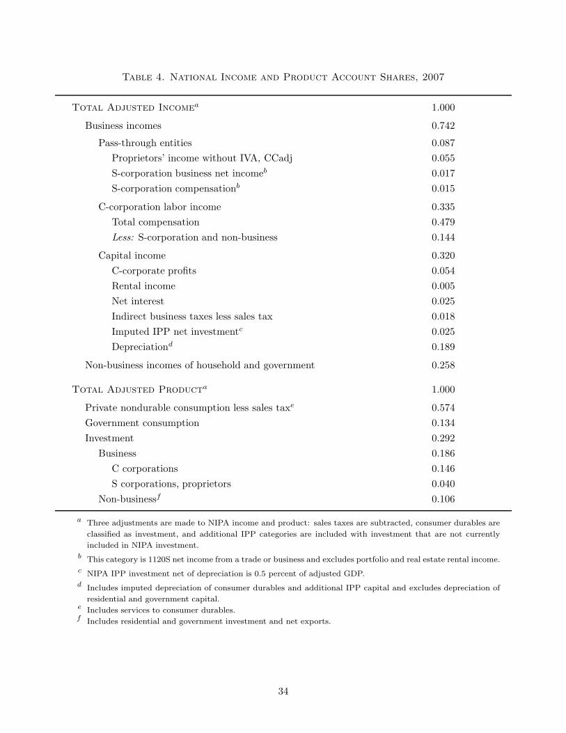
Table 4. National Income and Product Account Shares, 2007

Total Adjusted Incomea 1.000

Business incomes 0.742

Pass-through entities 0.087

Proprietors’ income without IVA, CCadj 0.055

S-corporation business net incomeb 0.017

S-corporation compensationb 0.015

C-corporation labor income 0.335

Total compensation 0.479

Less: S-corporation and non-business 0.144

Capital income 0.320

C-corporate profits 0.054

Rental income 0.005

Net interest 0.025

Indirect business taxes less sales tax 0.018

Imputed IPP net investmentc 0.025

Depreciationd 0.189

Non-business incomes of household and government 0.258

Total Adjusted Producta 1.000

Private nondurable consumption less sales taxe 0.574

Government consumption 0.134

Investment 0.292

Business 0.186

C corporations 0.146

S corporations, proprietors 0.040

Non-businessf 0.106

a Three adjustments are made to NIPA income and product: sales taxes are subtracted, consumer durables are

classified as investment, and additional IPP categories are included with investment that are not currently

included in NIPA investment.

b This category is 1120S net income from a trade or business and excludes portfolio and real estate rental income.

c NIPA IPP investment net of depreciation is 0.5 percent of adjusted GDP.

d Includes imputed depreciation of consumer durables and additional IPP capital and excludes depreciation of

residential and government capital.e Includes services to consumer durables.f Includes residential and government investment and net exports.

34

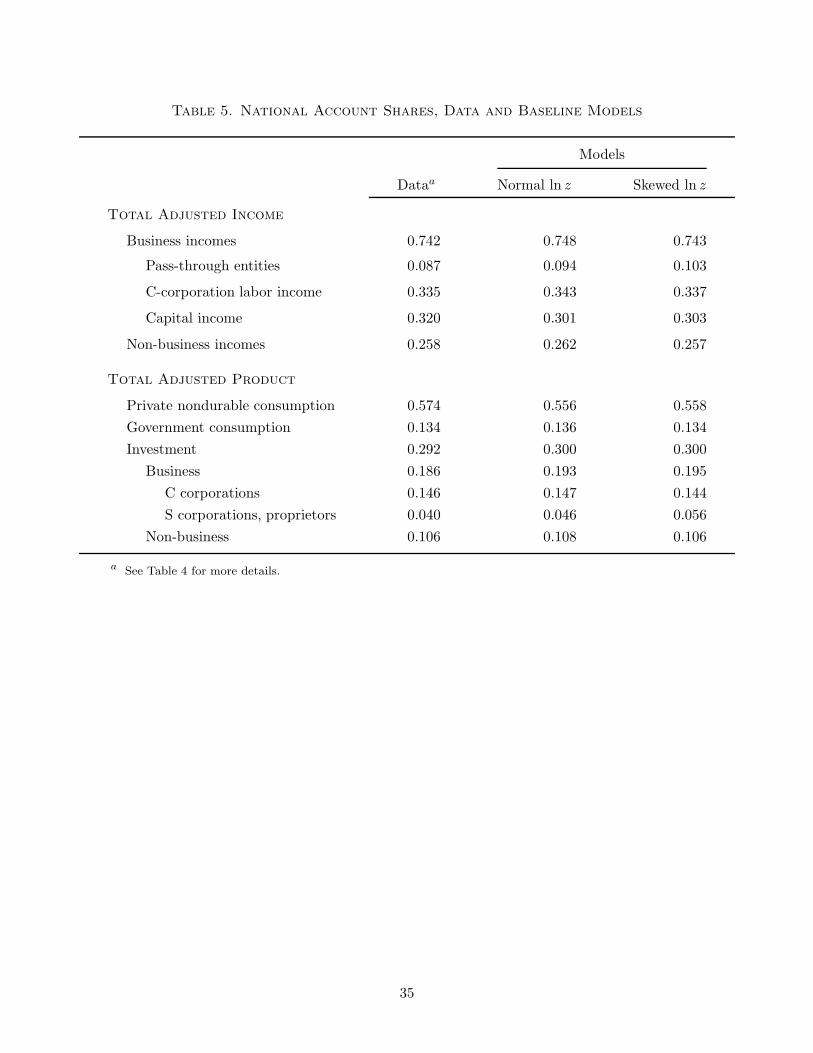
Table 5. National Account Shares, Data and Baseline Models

Models

Dataa Normal ln z Skewed ln z

Total Adjusted Income

Business incomes 0.742 0.748 0.743

Pass-through entities 0.087 0.094 0.103

C-corporation labor income 0.335 0.343 0.337

Capital income 0.320 0.301 0.303

Non-business incomes 0.258 0.262 0.257

Total Adjusted Product

Private nondurable consumption 0.574 0.556 0.558

Government consumption 0.134 0.136 0.134

Investment 0.292 0.300 0.300

Business 0.186 0.193 0.195

C corporations 0.146 0.147 0.144

S corporations, proprietors 0.040 0.046 0.056

Non-business 0.106 0.108 0.106

a See Table 4 for more details.

35

Table 6. Cross-Sectional Characteristics of Businessesa

Model Predictionsb

Business Owners All Individuals SCF

Intangible Sweat Gross Dividend Sweat Gross Dividend DividendStatistics Intensity Equity Return Yield Equity Return Yield Yield

Mean 0.51 1.07 11.4 3.5 1.17 4.6 1.4 307

Std. deviation 0.29 0.34 23.0 6.1 0.49 16.4 4.2 2,813

Percentiles:10th 0.20 0.71 -16.7 0.0 0.78 -10.8 0.0 0

50th 0.53 1.00 9.2 2.1 1.00 2.0 0.0 20

90th 0.97 1.50 44.5 10.2 1.89 17.7 7.9 240

95th 0.99 1.60 54.9 11.6 2.20 36.6 9.9 500

99th 1.00 2.27 87.4 21.4 3.66 66.8 19.1 5,000

a The model statistics are based on the case with skewed ln z productivity shocks.b The intangible intensity is the ratio of the business valuation Vb relative to the Vb plus the value of fixed assets

used in the business ks. The business valuation statistics for all individuals and business owners are reportedrelative to the median. The gross return on the business is the sum of the capital gain to sweat equity (Vb)plus the dividend yield, and both are in percentage terms. The dividend in this case is the share of revenuesto sweat equity (that is, φpys −x). The final column is the dividend yield (in percent) based on SCF data andis found by dividing net income by self-reported net worth for actively-managed businesses.

Table 7. Characteristics of Businesses, Sorted by Returnsa

Private Business ProductionReturn Age of IntangibleBounds Business Intensity Sweat capital Fixed assets Hours Output

−27.0, −15.3 11.2 0.67 0.37 1.14 0.06 0.27

−15.3, −0.6 15.5 0.65 0.35 2.01 0.09 0.48

−0.6, 2.3 17.8 0.71 0.27 0.67 0.04 0.16

2.3, 4.5 15.3 0.66 0.30 0.84 0.05 0.20

4.5, 11.9 15.4 0.47 0.33 3.50 0.15 0.83

11.9, 14.7 9.8 0.29 0.40 5.75 0.25 1.36

14.7, 19.4 5.1 0.35 0.31 4.62 0.23 1.09

19.4, 42.2 8.3 0.46 0.29 5.61 0.21 1.33

42.2, 208.8 6.3 0.34 0.32 4.34 0.27 1.64

a The model statistics are based on the case with skewed ln z productivity shocks.

36

Table 8. Tax Policy Counterfactuals, Percent Changesa

Greater Lower Rate, Lower Rates,Compliance Private Business All Businesses

Tax revenues 7.67 -5.28 -4.80

Prices

Wage (w) -.22 0.31 5.36

Relative price (p) 10.09 -5.26 -2.77

Interest rate (r) 0.68 -0.79 -0.53

Consumptions

Private business (∫

csi di) -14.19 8.84 8.97

C corporation (∫

cci di 4.01 -2.30 3.02

Investments

Sweat capital expenses (∫

xi di) -6.00 2.82 5.74

Private business capital (∫

xsi di) -5.81 3.50 6.20

C-corporate capital (xc) 2.36 -0.97 14.74

Outputs

Private business (∫

yi di) -14.19 8.84 8.97

C corporation (yc) 2.68 -1.42 6.45

GDP (yc + ynb + p∫

yi di) 0.58 -0.27 4.70

Hours

Sweat capital building (∫

hκi di) -23.56 15.48 13.31

Private business production (∫

hyi di) -22.51 15.30 12.87

C-corporate production (∫

niǫi di) 2.90 -1.72 1.03

Capital stocks

Sweat capital (∫

κi di) -17.97 11.06 9.78

Fixed assets (∫

ksi di) -5.81 3.50 6.20

C corporation (kc) 2.36 -0.97 14.74

Financial assets (∫

ai di)b 23.21 -16.07 -4.94

Sweat equity (Vb) -2.92 3.87 6.14

a The model statistics are based on the case with skewed ln z productivity shocks.

b Nonbusiness capital related to investment xnb is not included.

37