1

The Solar Wind Around Pluto (SWAP) Instrument Aboard New Horizons

D. McComas1,*, F. Allegrini1, F. Bagenal2, P. Casey1, P. Delamere2, D. Demkee1,

G. Dunn1, H. Elliott1, J. Hanley1, K. Johnson1, J. Langle3,1, G. Miller1, S. Pope1,

M. Reno1, B. Rodriguez1, N. Schwadron4,1, P. Valek1, S. Weidner1

1Southwest Research Institute®, San Antonio, Texas 78228-0510, U.S.A.

2University of Colorado, Boulder, Colorado 80309, U.S.A.

3Midwest Research Institute, Kansas City Missouri 64110, U.S.A.

4Boston University, Boston Massachusetts 02215, U.S.A.

( *author for correspondence, e-mail: DMcComas@swri.edu)

Abstract. The Solar Wind Around Pluto (SWAP) instrument on New Horizons will measure the

interaction between the solar wind and ions created by atmospheric loss from Pluto. These

measurements provide a characterization of the total loss rate and allow us to examine the complex

plasma interactions at Pluto for the first time. Constrained to fit within minimal resources, SWAP

is optimized to make plasma-ion measurements at all rotation angles as the New Horizons

spacecraft scans to image Pluto and Charon during the flyby. In order to meet these unique

requirements, we combined a cylindrically symmetric retarding potential analyzer (RPA) with

small deflectors, a top-hat analyzer, and a redundant/coincidence detection scheme. This

configuration allows for highly sensitive measurements and a controllable energy passband at all

scan angles of the spacecraft.

Keywords: solar wind, Pluto plasma interaction, pickup ions

1.0 Introduction

The New Horizons mission [Stern et al., 2007] will make the first up-close and

detailed observations of Pluto and its moons. These observations include

measurements of the solar wind interaction with Pluto. The Solar Wind Around

Pluto (SWAP) instrument is designed to measure the tenuous solar wind out at

~30 AU and its interaction with Pluto. SWAP directly addresses the Group 1

science objective for the New Horizons mission to “characterize the neutral

atmosphere of Pluto and its escape rate.” In addition, SWAP makes

measurements critical for the Group 2 objective of characterizing Pluto's

2

ionosphere and solar wind interaction. Finally, SWAP makes observations

relevant to two Group 3 science objectives for New Horizons, both in support of

characterizing the energetic particle environment of Pluto and Charon and in

searching for magnetic fields of Pluto and Charon.

As the solar wind approaches Pluto, it interacts with ions produced when Pluto’s

thin upper atmosphere escapes, streams away as neutral particles, and becomes

ionized. This pickup process slows the solar wind, and the type of interaction

varies greatly depending on the atmospheric escape rate. SWAP measurements

should provide the best estimate of the overall atmospheric escape rate at Pluto

and allow the first detailed examination of its plasma interactions with the solar

wind.

The SWAP observations are extremely challenging because the solar wind flux,

which falls off roughly as the square with distance, is approximately three orders

of magnitude lower at Pluto compared to typical solar wind fluxes observed near

Earth’s orbit. In addition, because the solar wind continues to cool as it propagates

out through the heliosphere, the solar wind beam becomes narrow in both angle

and energy.

The SWAP design was strongly driven by three constraints: 1) very low use of

spacecraft resources (mass, power, telemetry, etc.) as this is a non-core instrument

on a relatively small planetary mission; 2) very high sensitivity to measure the

solar wind and its interaction with Pluto out at ~30 AU, where the density is down

by a factor of ~1000 compared to 1 AU; and 3) the need to make observations

over a very large range of angles as the spacecraft constantly repoints its body-

mounted cameras during the flyby. Given these not-entirely-consistent design

drivers, we developed an entirely new design that combines elements of several

different previous plasma instruments. Together these components comprise the

SWAP instrument, which will measure the speed, density, and temperature of the

distant solar wind and its interaction with Pluto.

3

2.0 Scientific Background and Objectives

Only partly in jest, Dessler and Russell (1980) suggested that Pluto might act like

a colossal comet. The 1988 stellar occultation showed that Pluto’s tenuous

atmosphere could indeed be escaping (Hubbard et al., 1988; Elliot et al., 1989).

Applying basic cometary theories to Pluto, Bagenal and McNutt (1989) showed

that photoionization of escaping neutral molecules from Pluto’s atmosphere could

significantly alter the solar wind flow around Pluto for sufficiently large escape

rates. For large atmospheric escape rates, the interaction may be best described as

“comet-like,” with significant mass-loading over an extensive region; for small

escape rates the interaction is probably confined to a much smaller region,

creating a more “Venus-like” interaction (Luhmann et al., 1991), where electrical

currents in the gravitationally bound ionosphere deflect the solar wind flow.

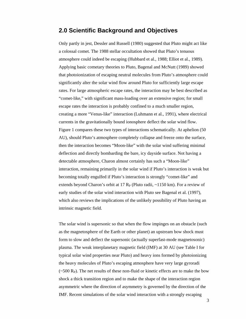
Figure 1 compares these two types of interactions schematically. At aphelion (50

AU), should Pluto’s atmosphere completely collapse and freeze onto the surface,

then the interaction becomes “Moon-like” with the solar wind suffering minimal

deflection and directly bombarding the bare, icy dayside surface. Not having a

detectable atmosphere, Charon almost certainly has such a “Moon-like”

interaction, remaining primarily in the solar wind if Pluto’s interaction is weak but

becoming totally engulfed if Pluto’s interaction is strongly “comet-like” and

extends beyond Charon’s orbit at 17 RP (Pluto radii, ~1150 km). For a review of

early studies of the solar wind interaction with Pluto see Bagenal et al. (1997),

which also reviews the implications of the unlikely possibility of Pluto having an

intrinsic magnetic field.

The solar wind is supersonic so that when the flow impinges on an obstacle (such

as the magnetosphere of the Earth or other planet) an upstream bow shock must

form to slow and deflect the supersonic (actually superfast-mode magnetosonic)

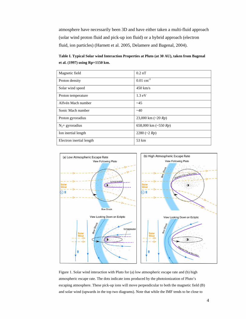
plasma. The weak interplanetary magnetic field (IMF) at 30 AU (see Table I for

typical solar wind properties near Pluto) and heavy ions formed by photoionizing

the heavy molecules of Pluto’s escaping atmosphere have very large gyroradi

(~500 RP). The net results of these non-fluid or kinetic effects are to make the bow

shock a thick transition region and to make the shape of the interaction region

asymmetric where the direction of asymmetry is governed by the direction of the

IMF. Recent simulations of the solar wind interaction with a strongly escaping

4

atmosphere have necessarily been 3D and have either taken a multi-fluid approach

(solar wind proton fluid and pick-up ion fluid) or a hybrid approach (electron

fluid, ion particles) (Harnett et al. 2005, Delamere and Bagenal, 2004).

Table I. Typical Solar wind Interaction Properties at Pluto (at 30 AU), taken from Bagenal

et al. (1997) using Rp=1150 km.

Magnetic field 0.2 nT

Proton density 0.01 cm-3

Solar wind speed 450 km/s

Proton temperature 1.3 eV

Alfvén Mach number ~45

Sonic Mach number ~40

Proton gyroradius 23,000 km (~20 Rp)

N2+ gyroradius 658,000 km (~550 Rp)

Ion inertial length 2280 (~2 Rp)

Electron inertial length 53 km

Figure 1. Solar wind interaction with Pluto for (a) low atmospheric escape rate and (b) high

atmospheric escape rate. The dots indicate ions produced by the photoionization of Pluto’s

escaping atmosphere. These pick-up ions will move perpendicular to both the magnetic field (B)

and solar wind (upwards in the top two diagrams). Note that while the IMF tends to be close to

5

tangential to Sun direction, the sign of the direction varies on timescales of days. The asymmetries

of the interaction will flip as the magnetic field changes direction.

Below we discuss how the current understanding of Pluto’s atmosphere leads us

to expect a more comet-like interaction at the time of the New Horizons flyby in

2015. Through measurements of bulk properties of the solar wind (flow, density,

temperature) as well as the energy distribution of solar wind and pick-up ions, the

SWAP instrument will not only characterize the solar wind interaction with Pluto

but will also allow us to determine the global rate of atmospheric escape.

In the comet-like scenario, variations on the scale of the interaction region can be

substantial over periods of days, and a factor of ~10 variations in the solar wind

flux can change the size of the interaction region from a few to more than 20 RP.

It is therefore critical to measure the solar wind for several solar rotations (~26

days per rotation) before and after the flyby in order to characterize the most

likely external solar wind properties during the actual encounter period.

Furthermore, since the strong asymmetry of the interaction depends on the

direction of the IMF, our analysis of SWAP data will need assistance from

increasingly capable models of solar wind structure based on plasma and

magnetometer data from spacecraft elsewhere in the solar system.

2.1 Atmospheric Escape

The exact nature of Pluto’s plasma interaction is critically dependent on the

hydrodynamic escape rate of the atmosphere from its weak gravity. Escaping

neutrals are photoionized by solar UV (or, less likely, suffer an ionizing collision).

Freshly ionized particles experience an electric field due to their motion relative to

the IMF (that is carried away from the Sun at ~400 km/s) and are accelerated by

this motional electric field, extracting momentum from the solar wind flow. This

electrodynamic interaction modifies the solar wind flow. Estimates of Pluto’s

atmospheric escape rate, Q, vary substantially: McNutt (1989) estimated 2.3-5.5 x

1027 s-1 for CH4-dominated outflow, Krasnopolsky (1999) found a hydrodynamic

outflow of N2 of 2.0-2.6 x 1027 s-1, while Tian and Toon (2005) derived values for

N2 escape as high as 2 x 1028 s-1. The nature of the plasma interaction varies

considerably over this range of escape rates since the scale of the interaction is

proportional to Q (Bagenal and McNutt, 1989).

6

Hydrodynamic escape of an atmosphere occurs when the atmospheric gases in the

upper atmosphere (in the vicinity of the exobase) are heated significantly (so that

the thermal speed is comparable to the local sound speed). Krasnopolsky and

Cruikshank (1999) reviewed the photochemistry of Pluto’s atmosphere while

Krasnopolsky (1999) summarized approaches taken in modeling the complexities

of hydrodynamic escape at Pluto. Earlier models approximated all the heating that

occurs in a thin layer of the atmosphere. Recently, however, Tian and Toon

(2005) developed a model that includes a distributed heating function appropriate

for EUV absorption by the dominant molecule N2 relatively high in Pluto’s

atmosphere, which leads to larger escape rates. These authors derive an exobase

height of 10-13 RP and transonic point of ~30 RP. The fact that even with

significant heating the escape speed (<100 m/s) is subsonic at the exobase is

consistent with what Krasnopolsky (1999) called “slow hydrodynamic escape.”

Nevertheless, an exobase at 10-13 RP implies a very extended atmosphere, and the

present New Horizons trajectory with a currently planned closest approach of ~9

RP, may well briefly dip below the exobase.

Tian and Toon (2005) modeled the effects of variations in (i) EUV flux over the

solar cycle, and (ii) Pluto’s distance from the Sun, in order to estimate the

variability of atmospheric escape over full Pluto orbit. They found escape rates

varying from 2 x 1028 s-1 (for Pluto at 30 AU and solar maximum activity) to 1 x

1028 s-1(for Pluto at 40 AU and solar minimum). These authors, however, were not

able to find a stable solution for atmospheric escape at the low heating levels

appropriate for aphelion (50 AU). Whether Pluto retains a stable atmosphere

through aphelion or not remains an open issue. Surprisingly, recent occultation

measurements suggest that Pluto’s atmosphere has been expanding rather than

collapsing as Pluto recedes from the Sun (Elliot et al., 2003).

Assuming the current estimates for the escaping atmosphere have persisted over

the age of the solar system, Pluto would have lost the equivalent of a layer of N2

ice 0.5 to 3 km thick from the entire surface. While this is a relatively small

fraction of the mass of Pluto, the loss is certainly sufficient to have affected the

surface topography.

7

2.2 Solar wind Interaction at High Atmospheric Escape

Galaav et al. (1985) derived a size for the interaction region (over which

significant momentum would be extracted from the solar wind) for comets that is

proportional to Q and inversely proportional to the solar wind flux, nswVsw.

Bagenal and McNutt (1989) applied this simple scaling law to Pluto and found

that for typical solar wind conditions and photoionization of CH4 or N2, the scale

size of the dayside interaction region, RSO (the “stand-off” distance) is RSO/RP =

Q/Q0) where Q0 is 1.5 x 1027 s-1. Applying the upper range of atmospheric escape

rates discussed above, one finds RSO = 6-13 RP for 1-2 x 1027 s-1. (assuming an

escape speed of 100 m/s). Note that these simple calculations assume the exobase

is close to the planet. Tian and Toon (2005) suggest that the exobase may be as

high as 10-13 Rp, in which case the standoff distance would be expanded

accordingly. Nevertheless, the linear dependence on solar flux means that the

typical factor of ~2 variation in solar wind density would produce a similar

variation in RSO, often extending the interaction region beyond the orbit of Charon

at 17 RP.

The above simple scaling is based on a fluid approach that is appropriate for

cometary interactions in the inner solar system. The weak IMF at 30 AU (see

Table I) means that ion kinetic effects are crucial at Pluto due to the large pickup-

ion gyroradius (Kecskemety and Cravens, 1993) and the large turning distance for

the solar wind protons (Bagenal et al., 1997).

Previous models of weakly outgassing (i.e. production rates, Q ~1027 s-1) bodies

used two-dimensional, two-ion fluid and/or hybrid simulations (Bogdanov et al.,

1996; Sauer et al., 1997; Hopcroft and Chapman, 2001). All of these models

showed the formation of asymmetric plasma structures. Sauer et al. (1997)

specifically investigated the Pluto plasma interaction with two-dimensional

models for Q > 1027 s-1. While the two-dimensional models provide a good

qualitative description of the interaction, the quantitative details of the plasma

coupling (i.e. momentum transfer) require three-dimensional models. More

recently, Lipatov et al. (2002) performed a three-dimensional hybrid code

simulation of the solar wind with weak comets and illustrated the dependence of

gas production rates (6.2 x 1026 s-1 < Q < 1028 s-1) on plasma structure. However,

8

these results are applicable to 1 AU where the ions are more strongly magnetized

compared to the situation at 30 AU where the IMF is very weak and the solar

wind is tenuous.

Delamere and Bagenal (2004) modeled the kinetic interaction of the solar wind

with Pluto’s escaping atmosphere using a hybrid simulation that treats the pick-up

ions and solar wind protons as particles and the electrons as a massless fluid. A

hybrid code is a reasonable approach for a system with scale sizes ranging from

the ion inertial length of the solar wind protons (~2 RP) to the pick-up ion (N2+)

gyroradius (~500 RP). Figure 2 shows a schematic of the ion motion near Pluto in

this kinetic regime. Note the asymmetry of the interaction imposed by the

direction of the magnetic field in the solar wind (Bsw).

Figure 2. Schematic of ion motion near Pluto’s interaction region. Pickup ions move initially in the

direction of the solar wind convection electric field (+y) and the solar wind flow is deflected in the

-y direction, consistent with momentum conservation.

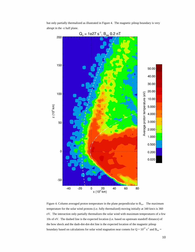
Figures 3, 4 and 5 show the density, temperature, and bulk flow resulting from

hybrid simulations for an atmospheric escape rate of Q = 1 x 1027 s-1 |B| = 0.2 nT

and an atmospheric escape speed of 100 m/s (Delamere and Bagenal, 2004, 2007)

in the same geometry depicted in Figure 2 (upstream solar wind flow from the left

and IMF pointing out of the page). The main features of the interaction are a

broad region of proton heating extending ~20 RP upstream of Pluto consistent

with the expected location of a bow shock. The kinetic energy of the solar wind

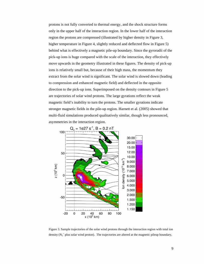
9

protons is not fully converted to thermal energy, and the shock structure forms

only in the upper half of the interaction region. In the lower half of the interaction

region the protons are compressed (illustrated by higher density in Figure 3,

higher temperature in Figure 4, slightly reduced and deflected flow in Figure 5)

behind what is effectively a magnetic pile-up boundary. Since the gyroradii of the

pick-up ions is huge compared with the scale of the interaction, they effectively

move upwards in the geometry illustrated in these figures. The density of pick-up

ions is relatively small but, because of their high mass, the momentum they

extract from the solar wind is significant. The solar wind is slowed down (leading

to compression and enhanced magnetic field) and deflected in the opposite

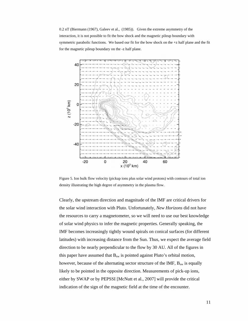
direction to the pick-up ions. Superimposed on the density contours in Figure 5

are trajectories of solar wind protons. The large gyrations reflect the weak

magnetic field’s inability to turn the protons. The smaller gyrations indicate

stronger magnetic fields in the pile-up region. Harnett et al. (2005) showed that

multi-fluid simulations produced qualitatively similar, though less pronounced,

asymmetries in the interaction region.

Figure 3. Sample trajectories of the solar wind protons through the interaction region with total ion

density (N2+ plus solar wind proton). The trajectories are altered at the magnetic pileup boundary,

10

but only partially thermalized as illustrated in Figure 4. The magnetic pileup boundary is very

abrupt in the -z half plane.

Figure 4. Column averaged proton temperature in the plane perpendicular to Bsw. The maximum

temperature for the solar wind protons (i.e. fully thermalized) moving initially at 340 km/s is 360

eV. The interaction only partially thermalizes the solar wind with maximum temperatures of a few

10s of eV. The dashed line is the expected location (i.e. based on upstream standoff distance) of

the bow shock and the dash-dot-dot-dot line is the expected location of the magnetic pileup

boundary based on calculations for solar wind stagnation near comets for Q = 1027 s-1 and Bsw =

11

0.2 nT (Biermann (1967), Galeev et al., (1985)). Given the extreme asymmetry of the

interaction, it is not possible to fit the bow shock and the magnetic pileup boundary with

symmetric parabolic functions. We based our fit for the bow shock on the +z half plane and the fit

for the magnetic pileup boundary on the -z half plane.

Figure 5. Ion bulk flow velocity (pickup ions plus solar wind protons) with contours of total ion

density illustrating the high degree of asymmetry in the plasma flow.

Clearly, the upstream direction and magnitude of the IMF are critical drivers for

the solar wind interaction with Pluto. Unfortunately, New Horizons did not have

the resources to carry a magnetometer, so we will need to use our best knowledge

of solar wind physics to infer the magnetic properties. Generally speaking, the

IMF becomes increasingly tightly wound spirals on conical surfaces (for different

latitudes) with increasing distance from the Sun. Thus, we expect the average field

direction to be nearly perpendicular to the flow by 30 AU. All of the figures in

this paper have assumed that Bsw is pointed against Pluto’s orbital motion,

however, because of the alternating sector structure of the IMF, Bsw is equally

likely to be pointed in the opposite direction. Measurements of pick-up ions,

either by SWAP or by PEPSSI [McNutt et al., 2007] will provide the critical

indication of the sign of the magnetic field at the time of the encounter.

12

2.3 Solar wind Interaction at Low Atmospheric Escape

If Pluto’s escape rate is less than ~1027 s-1, with few pick-up ions to slow it down,

then the solar wind is expected to penetrate close to Pluto and impinge directly

onto its ionosphere. Strictly speaking, the “obstacle” that deflects the solar wind is

this interaction produced by the electrical currents induced in the ionosphere.

Such an interaction would be similar to the solar wind interaction with Venus or

the magnetospheric interaction with Titan (Luhmann et al. 1999). The

photochemistry of Pluto’s upper atmosphere and ionosphere modeled by both

Krasnopolsky and Cruikshank (1999) and by Ip et al. (2000) show peak

ionospheric densities of a few x 103 cm-3 at altitudes of ~1000 km above the

surface of Pluto. They find the main ionospheric ion to be H2CN+.

The solar wind deflection and any pick-up ions will be significantly harder to

measure on the New Horizons flyby in the case of a Venus-like interaction.

However, the broad nature of the bow shock and the large gyroradii of any ions

beyond the ionosphere should still produce detectable signatures several radii

away from Pluto.

2.4 Solar wind Interaction at Aphelion

It is not clear whether the atmosphere of Pluto completely collapses onto the

surface when Pluto reaches aphelion. In the absence of a significant atmosphere

Pluto will have a “Moon-like” interaction, as is expected for its moon Charon. In

this type of interaction, the solar wind is absorbed on the sunlit side and the IMF

diffuses through the non-conducting bodies, generating an extremely hard vacuum

in the cavity behind. It seems unlikely that at temperatures below 40K Pluto’s icy

outer layers could be electrically conducting. But should they have significant

conductivity, the plasma interaction may be similar to the solar wind/asteroid

interaction described by Wang and Kivelson (1996), Omidi et al. (2002), and

Blanco-Cano et al. (2003). If the dimensions of the obstacle are small compared to

the ion inertial length, then the interaction is mediated by the whistler mode.

Comparison of Galileo observations of asteroid-associated perturbations with

numerical models confirm the whistler-mode interaction. Magnetohydrodynamic

shock waves are absent with small obstacles as compressional waves can only

exist on size scales larger than the ion inertial length. Pluto represents a possible

13

intermediate case if the interaction region is limited to an area close to the planet

as the solar wind proton inertial length is roughly 2 RP.

2.5 Heliospheric Pickup Protons

In addition to the primary science of measuring the solar wind interaction with

Pluto, SWAP may afford an excellent opportunity to measure heliospheric pickup

protons on its way out through the heliosphere, en route to Pluto (and beyond).

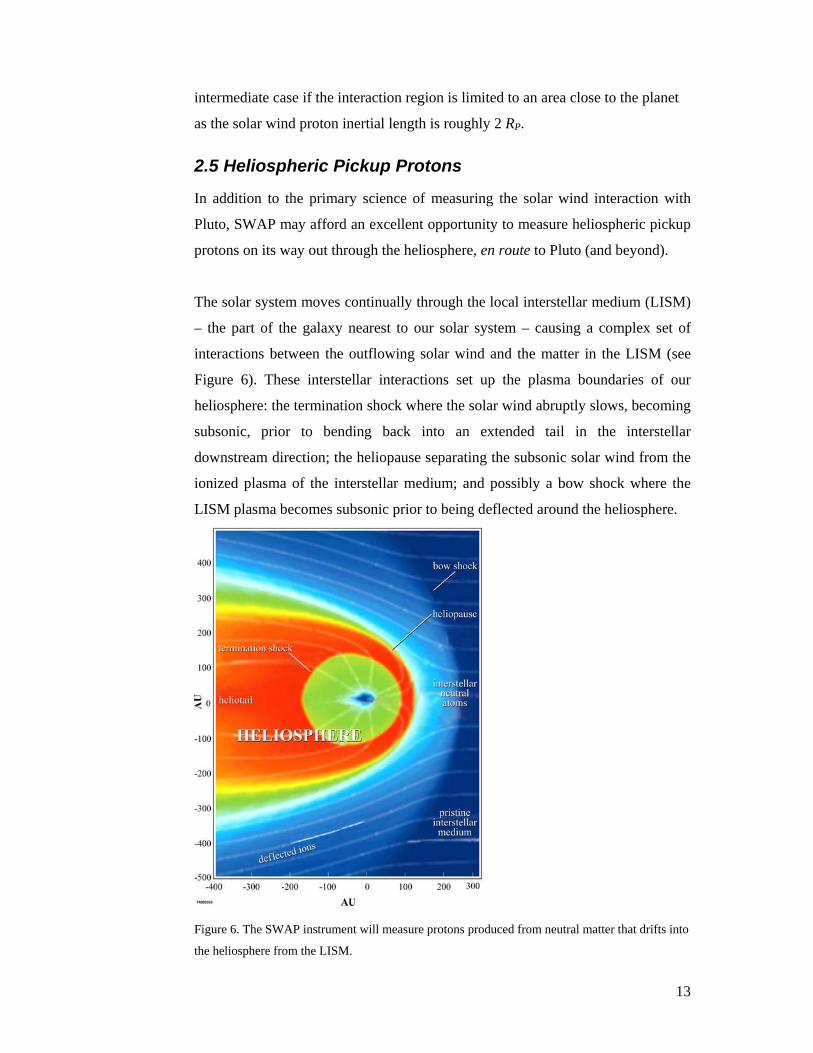
The solar system moves continually through the local interstellar medium (LISM)

– the part of the galaxy nearest to our solar system – causing a complex set of

interactions between the outflowing solar wind and the matter in the LISM (see

Figure 6). These interstellar interactions set up the plasma boundaries of our

heliosphere: the termination shock where the solar wind abruptly slows, becoming

subsonic, prior to bending back into an extended tail in the interstellar

downstream direction; the heliopause separating the subsonic solar wind from the

ionized plasma of the interstellar medium; and possibly a bow shock where the

LISM plasma becomes subsonic prior to being deflected around the heliosphere.

Figure 6. The SWAP instrument will measure protons produced from neutral matter that drifts into

the heliosphere from the LISM.

14

Interstellar atoms, predominantly H, continually drift into and through the

heliosphere, and due to their neutrality are unimpeded by the solar wind. The H

atoms on trajectories toward the Sun move into regions of increasingly dense solar

wind and higher levels of radiation, enhancing the probability of ionization

through charge-exchange or photo-ionization. The vast majority of interstellar H

atoms that penetrate inside of 4 AU become ionized and incorporated into the

solar wind flow. Upon ionization, the newborn ion begins essentially at rest in the

reference frame of the spacecraft and Sun. Just like for planetary pickup ions, as

described above, because the moving solar wind carries frozen-in magnetic field

lines, the newborn ions encounter a motional electric field (-vsw x B) exerted by

the solar wind and become picked-up and carried outward with the solar wind. As

they move outward, the pickup ions also scatter due to magnetic inhomogeneities

in the IMF, forming an almost spherical ring distribution in velocity space. As

measured by spacecraft, these interstellar pickup-ion distributions are essentially

flat for speeds less than 2 vsw, then drop off at speeds above this limit (Gloeckler

et al., 1995).

The first interstellar pickup ions discovered (Möbius et al., 1985) were He+

created by ionization of interstellar neutral He that penetrated within 1 AU of the

Sun. The composition and velocity space-resolved measurements by the SWICS

experiment on Ulysses (Gloeckler et al., 1992) made it possible to explore pickup

ions from 1.35-5.4 AU in great detail. The review by Gloeckler and Geiss (1998)

provides an excellent summary of these pickup-ion observations. The

observations include the most abundant pickup ion, H+, second most abundant,

He+, and several other interstellar pickup-ion species, N+, O+, and Ne+ (Geiss et

al., 1994). The SWICS team demonstrated the existence of pickup distributions of

He++, which is produced largely by double charge exchange of atomic He with

solar wind alpha particles (Gloeckler et al., 1997) and rare 3He+ pickup ions. In

addition to the interstellar pickup ions, SWICS distributions showed that the

majority of the C+ and a fraction of the O+ and N+ are produced by an additional

“inner source” of neutral atoms located near the Sun (Geiss et al., 1995). The

inner–source, velocity-space distributions are significantly modified as they cool

over the solar wind’s transition from the near-Sun source to several AU where

they were observed (Schwadron et al., 2000).

15

Ulysses/SWICS also observed the ubiquity of pickup-ion tails in slow solar wind

(Gloeckler et al., 1994; Schwadron et al., 1996; Gloeckler, 1999). These tails do

not correlate strongly with the presence of shock but with compressive

magnetosonic waves, showing that pickup ions are subject to strong statistical

acceleration through processes such as transit-time damping of magnetosonic

waves in slow solar wind (Schwadron et al., 1996; Fisk et al., 2000).

Prior to Ulysses, it was expected that pickup-ion distributions should be fairly

isotropic due to pitch-angle scattering from background turbulence and self-

generated waves (Lee and Ip, 1987). Instead, pickup-ion distributions were

observed to be highly anisotropic (Gloeckler et al., 1995) with scattering mean

free paths ~1 AU; the most likely cause is the inhibition of scattering through 90°

pitch angle (Fisk et al., 1997). Although this lack of scattering is not fully

understood, it has been shown that the turbulence of the wind has a strong 2-D

component (Matthaeus et al., 1990; Bieber et al., 1996) that is ineffective for

pickup-ion scattering (Bieber et al., 1994; Zank et al., 1998). Accurate pickup-ion

models have been devised that take into account the long-scattering mean free

path (e.g., Isenberg, 1997; Schwadron, 1998).

Interestingly, the same self-generated turbulence caused by pickup-ion scattering

has been considered an energy source for heating the solar wind (Zank et al.,

1996; Matthaeus et al., 1999). These theories for the turbulent heating of solar

wind take into account both the pickup-ion driven turbulence, which is

predominant outside of ~8 AU, and wind shear. Smith et al. (2001), Smith et al.

(2006) have rigorously tested the heating models using data from Voyager 2 and

Pioneer 11, and improved models of the pickup-ion scattering and associated

wave excitation (Isenberg et al., 2005) have lead to remarkable agreement

between data and theory.

Charge-exchange interstellar hydrogen and solar wind protons lead to a complex

interaction near the nose of the heliosheath, where a so-called hydrogen wall is

formed from slowed interstellar hydrogen atoms and charge-exchanged solar wind

protons. These interactions cause the removal or filtration of a fraction of the

16

penetrating interstellar hydrogen atoms (e.g., Baranov and Malama, 1995). The

solar radiation pressure and the rates of photo-ionization and charge exchange

vary with solar latitude and over the solar cycle. Sophisticated models of

interstellar neutral atoms have been developed to take these effects into account

(e.g., Izmodenov et al., 1999).

Cassini was the first spacecraft to measure pickup ions in the interstellar

downstream region of the heliosphere beyond 1 AU (McComas et al., 2004a).

Both interstellar pickup H+ and He+ were identified with the familiar cutoff in

velocity space at twice the solar wind speed. Observed enhancements in the

pickup He+ were consistent with gravitational focusing by the Sun. Further, the

first in situ observations were reported of the interstellar hydrogen shadow caused

by depletion of H atoms in the downstream region due to the outward force of

radiation pressure (which exceeded the gravitational force at the time of

observation) and the high probability of ionization for atoms that must pass close

to the Sun to move behind it.

The trajectory of New Horizons takes the spacecraft out to Pluto, which is

currently toward the nose of the heliosphere. Figure 7 shows the distribution

functions of pickup protons and solar wind protons in the spacecraft frame. We

have used a kappa distribution for the solar wind protons (e.g., Vasyliunas, 1968;

Collier, 1993) (with a kappa ~ 3, which is typical), and a density that falls off as

R-2 from a 1 AU density of 5 cm-3 and temperatures consistent with observations

(e.g., Smith et al., 2001). For the pickup protons, we have taken a steady-state

distribution that includes convection, adiabatic cooling in the radially expanding

flow (Vasyliunas and Siscoe, 1976). The proton-pickup rate at each location is the

local ionization rate time the neutral density solved using the “hot” model (Fahr,

1971; Thomas, 1978; Wu and Judge, 1979), which accounts for gravitational

focusing by the Sun, ionization loss, and the finite temperature of incoming

neutral atoms. We have taken an interstellar density near the termination shock of

0.1 cm-3, and neutral temperature of 11 000 K, a neutral inflow speed of 22 km/s,

an ionization rate of 7 x 10-7 (referenced at 1 AU). We have also taken the force of

radiation pressure to be comparable to gravity (µ ~ 1). The top panel in Figure 7

shows that solar wind protons are typically comparable to pickup protons near 5

17

AU. The pickup protons are observable near the knee, so long as the solar wind is

not significantly hotter or has significantly broader tails than those shown. Since

the plasma near the ecliptic plane is typically disturbed near 5 AU, detecting

pickup protons is possible, but often obscured by the solar wind. As we move out

toward the nose of the heliosphere, the situation changes. The solar wind density

falls off with the square of distance (while the pickup protons fall off only as R-1)

and cools. Both of these effects make it much easier to detect “clean” pickup-

proton distributions. The distribution functions shown in Figure 7, may be readily

used to predict SWAP’s observed count rates from pickup protons. Because of

SWAP’s large geometric factor, these count rates are typically 0.3-0.8 protons/s at

30 AU. This range could be 2-5 proton/s if we use the detector geometric factor as

opposed to the COIN geometric factor (used to get 0.3-0.8 proton/s). These rates

are quite large and will allow measurement of highly resolved distribution

functions over very short observation periods (on the scale of hours).

18

Figure 7. Pickup-proton (solid curves) and solar wind (dashed curves) distribution functions

shown with distance from the Sun toward the nose of the heliosphere. The pickup-proton

distribution functions become more and more prominent compared to the cooled solar wind

distributions further out in the heliosphere.

The unique trajectory of New Horizons combined with SWAP’s capability of

pickup-proton measurement should enable it to address some fascinating issues:

• SWAP will measure pickup protons in the region toward the nose of the

heliosphere where interstellar hydrogen atoms have undergone relatively

little interaction through charge exchange with the solar wind inside the

termination shock. These measurements should provide best estimates for

the hydrogen density immediately after filtration in the hydrogen wall at

the nose of the heliosphere. The measurements will also provide more

information about the hydrogen parameters (density, temperature and

neutral bulk velocity) in the LISM.

• SWAP will simultaneously measure the solar wind proton distributions

and pickup-ion proton distributions over an extremely large range of

heliocentric distances, providing direct tests of models of pickup-ion-

driven turbulence and associated heating of the solar wind.

• SWAP will directly measure the evolution of accelerated pickup-ion tails

over a broad range of distances from the Sun. These measurements will

lead to important discoveries about the pre-acceleration of pickup protons,

which naturally feeds into particle acceleration at the termination shock

and the formation of Anomalous Cosmic Rays.

The distribution functions measured by SWAP will allow investigation of possible

sources (other than interstellar) of pickup ions. For example, it is thought that an

Outer Source of pickup ions may be caused by the interaction of solar wind with

dust grains from the Kuiper Belt (Schwadron et al., 2003). The Outer Source is

likely to be far more variable in space and time than the interstellar source.

3.0 Instrument Description

The SWAP electro-optics consists of 1) a retarding potential analyzer (RPA); 2) a

deflector (DFL); and 3) an electrostatic analyzer (ESA). Collectively, these

19

elements select the angles and energies of the solar wind to be measured. Solar

wind ions selected by the electro-optics are then registered with a coincidence

detector system. Figure 8 schematically depicts the SWAP principle electro-

optics. Ions enter through the RPA with all ions having energy per charge less

than the RPA voltage being rejected by this hi-pass filter. Ions entering at angles

from above horizontal in this figure can be deflected in to the subsequent electro-

optics by applying a voltage to the deflector ring. Ions with E/q greater than the

RPA voltage are then selected by the ESA, which rejects ions outside the selected

E/q range as well as UV light and neutral particles.

Figure 8. Schematic diagram of the SWAP electro-optics including RPA, deflector, ESA, and

detector section.

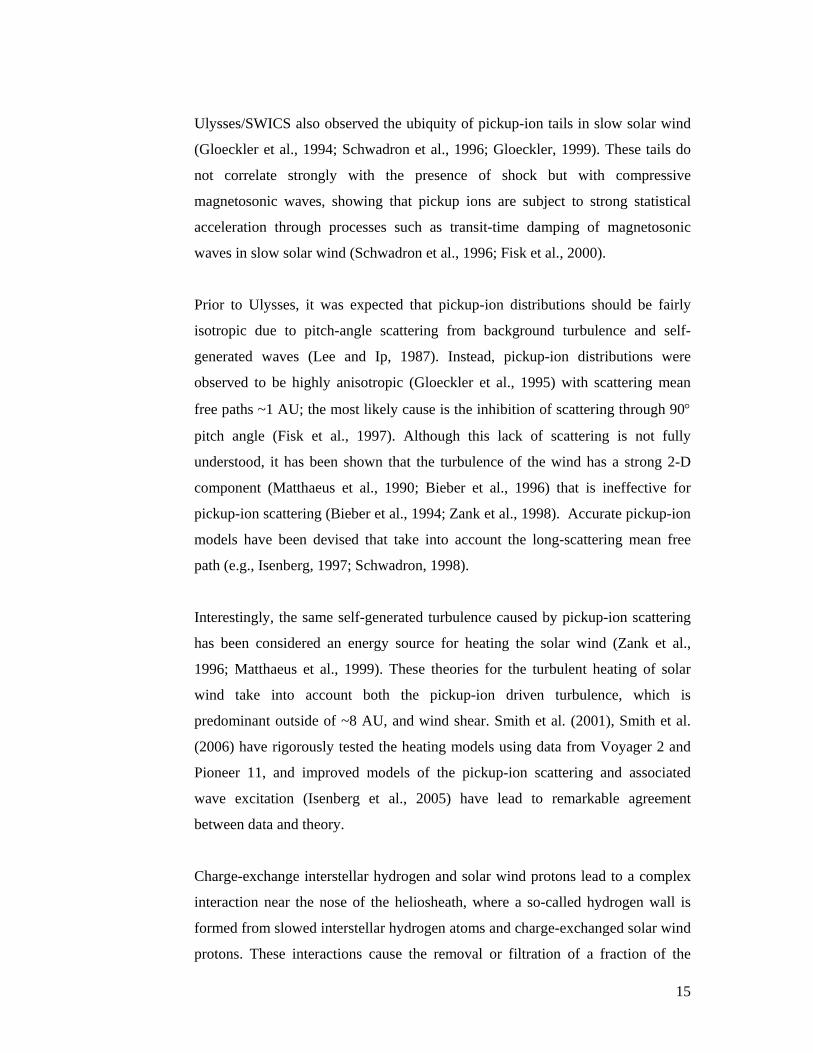
Figure 9 schematically shows how SWAP’s ESA and RPA are used together to

select the E/q passband. When the RPA is off, the passband is determined solely

by the ESA, which has an 8.5% FWHM resolution (top panel). At increasing RPA

values for a given ESA setting, the passband is cutoff in a variable “shark-fin”

shape, allowing roughly two decades decreased sensitivity (middle panel). Finally,

differentiating adjacent RPA/ESA combinations, or better yet deconvolving

20

multiple combinations, provides high resolution differential measurements of the

incident beam.

Figure 9. SWAP principle of operation. Different combinations of RPA and ESA settings provide

for a variable E/q passband. Multiple combinations of settings can be differentiated to produce

very high-resolution measurements.

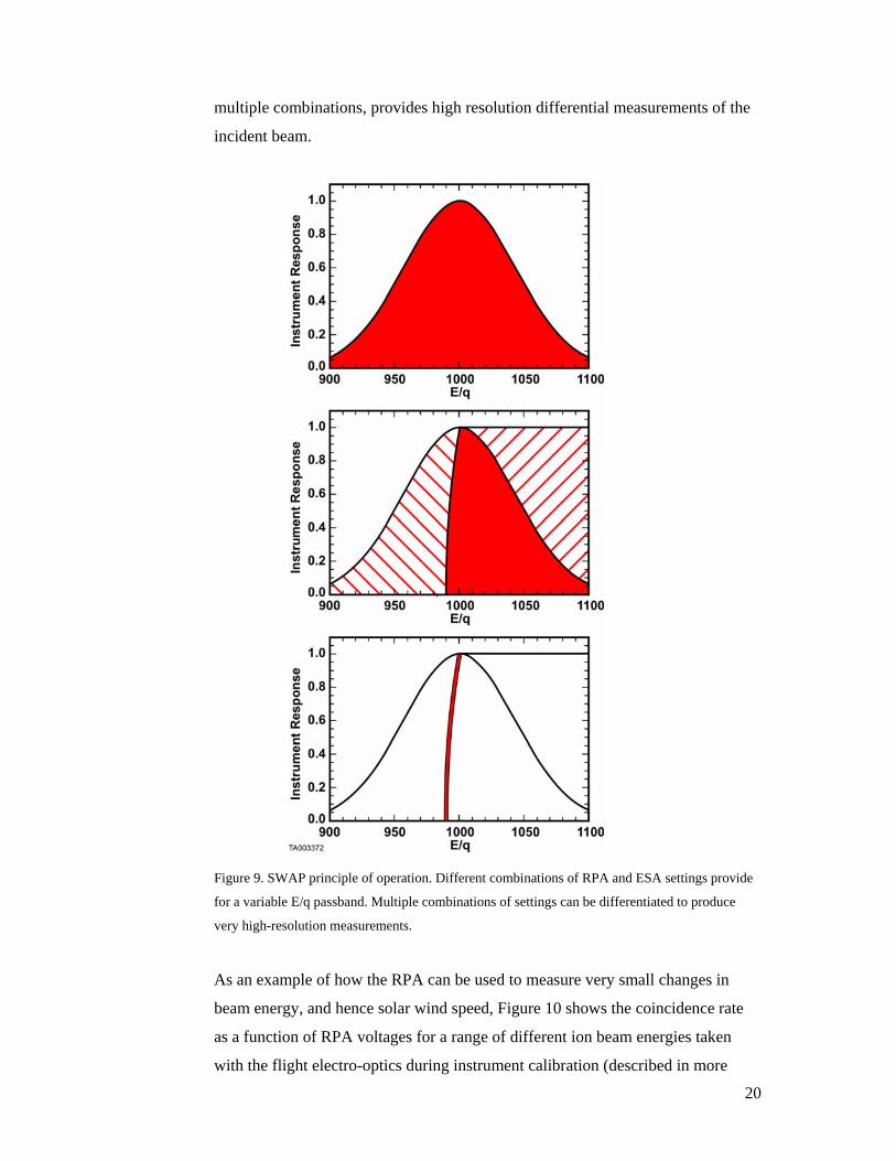
As an example of how the RPA can be used to measure very small changes in

beam energy, and hence solar wind speed, Figure 10 shows the coincidence rate

as a function of RPA voltages for a range of different ion beam energies taken

with the flight electro-optics during instrument calibration (described in more

21

detail below). A small subset of the full energy range of SWAP (990 to 1010 eV)

is shown to highlight the energy resolution possible by this instrument. For each

scan, the coincidence count rate is normalized to the rate when the RPA voltage is

set at zero to take into account the differences in the ion beam flux. Differences in

the ion energy as small as 1-2 eV are distinguishable at typical solar wind energies

of ~1000 eV.

Figure 10. RPA resolution of ion beams with energies from 990-1010 eV. Each RPA scan shown

was taken with the beam incident normal to the RPA. Deconvolution of such curves should make

changes in beam energy as small as 1-2 eV possible.

The transmitted ions enter the detector section, which employs an ultra-thin

carbon foil and two channel electron multipliers (CEMs) to make a coincidence

measurement of both the primary particle and the secondary electrons generated

when the primary particle passes through an ultra-thin carbon foil. Charge

amplifiers (CHAMPs) service the two CEMs and transmit digital pulses when

events are detected. High voltage power supplies (HVPS) provide power for the

CEMs and sweep the voltages on the electro-optics. The control board processes

the pulses from the CHAMPs, controls the sweeping of the high voltages,

digitizes the housekeeping data, creates telemetry packets for transmission,

accepts commands, and converts spacecraft power into the secondary voltages

22

required by the instrument. Key properties of the SWAP instrument are given in

Table II. The block diagram for SWAP is shown in Figure 11.

Table II. Properties of the SWAP instrument

Field of View 276° x 10° (deflectable >15° toward -Z) Energy Range ESA (bin centers) RPA

35 eV to 7.5 keV 0 to 2000 V

Energy Resolution ESA (∆E/E) RPA

0.085 FWHM 0.5 V steps (high resolution requires deconvolution)

ESA factor (beam energy / ESA voltage)

1.88

Dynamic range ~106 Geometric Factor (Hot Plasma)

1.8x10-3 cm2 sr eV/eV

Time Resolution Full energy range and 1) detailed peak measurements or 2) additional full energy sweep each 64s (128 steps with 0.39s accumulation times)

Mass 3.29 kg Volume 0.011 m3 Power 2.84 W Telemetry <1 - 280 bps

Figure 11. SWAP Block Diagram

23

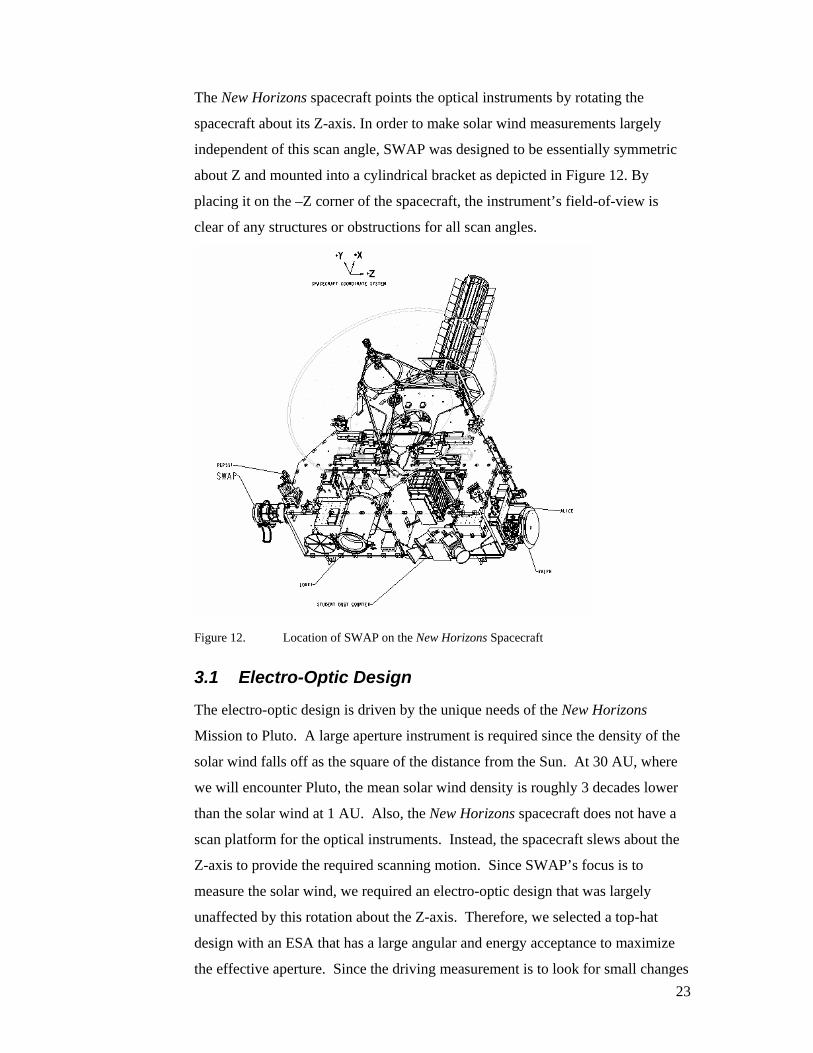
The New Horizons spacecraft points the optical instruments by rotating the

spacecraft about its Z-axis. In order to make solar wind measurements largely

independent of this scan angle, SWAP was designed to be essentially symmetric

about Z and mounted into a cylindrical bracket as depicted in Figure 12. By

placing it on the –Z corner of the spacecraft, the instrument’s field-of-view is

clear of any structures or obstructions for all scan angles.

Figure 12. Location of SWAP on the New Horizons Spacecraft

3.1 Electro-Optic Design

The electro-optic design is driven by the unique needs of the New Horizons

Mission to Pluto. A large aperture instrument is required since the density of the

solar wind falls off as the square of the distance from the Sun. At 30 AU, where

we will encounter Pluto, the mean solar wind density is roughly 3 decades lower

than the solar wind at 1 AU. Also, the New Horizons spacecraft does not have a

scan platform for the optical instruments. Instead, the spacecraft slews about the

Z-axis to provide the required scanning motion. Since SWAP’s focus is to

measure the solar wind, we required an electro-optic design that was largely

unaffected by this rotation about the Z-axis. Therefore, we selected a top-hat

design with an ESA that has a large angular and energy acceptance to maximize

the effective aperture. Since the driving measurement is to look for small changes

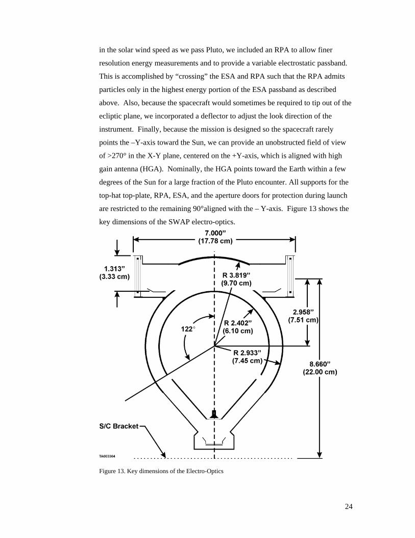
24

in the solar wind speed as we pass Pluto, we included an RPA to allow finer

resolution energy measurements and to provide a variable electrostatic passband.

This is accomplished by “crossing” the ESA and RPA such that the RPA admits

particles only in the highest energy portion of the ESA passband as described

above. Also, because the spacecraft would sometimes be required to tip out of the

ecliptic plane, we incorporated a deflector to adjust the look direction of the

instrument. Finally, because the mission is designed so the spacecraft rarely

points the –Y-axis toward the Sun, we can provide an unobstructed field of view

of >270° in the X-Y plane, centered on the +Y-axis, which is aligned with high

gain antenna (HGA). Nominally, the HGA points toward the Earth within a few

degrees of the Sun for a large fraction of the Pluto encounter. All supports for the

top-hat top-plate, RPA, ESA, and the aperture doors for protection during launch

are restricted to the remaining 90°aligned with the – Y-axis. Figure 13 shows the

key dimensions of the SWAP electro-optics.

Figure 13. Key dimensions of the Electro-Optics

25

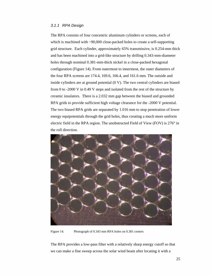
3.1.1 RPA Design

The RPA consists of four concentric aluminum cylinders or screens, each of

which is machined with ~90,000 close-packed holes to create a self-supporting

grid structure. Each cylinder, approximately 65% transmissive, is 0.254-mm thick

and has been machined into a grid-like structure by drilling 0.343-mm-diameter

holes through nominal 0.381-mm-thick nickel in a close-packed hexagonal

configuration (Figure 14). From outermost to innermost, the outer diameters of

the four RPA screens are 174.4, 169.6, 166.4, and 161.6 mm. The outside and

inside cylinders are at ground potential (0 V). The two central cylinders are biased

from 0 to -2000 V in 0.49 V steps and isolated from the rest of the structure by

ceramic insulators. There is a 2.032 mm gap between the biased and grounded

RPA grids to provide sufficient high voltage clearance for the -2000 V potential.

The two biased RPA grids are separated by 1.016 mm to stop penetration of lower

energy equipotentials through the grid holes, thus creating a much more uniform

electric field in the RPA region. The unobstructed Field of View (FOV) is 276° in

the roll direction.

Figure 14. Photograph of 0.343 mm RPA holes on 0.381 centers

The RPA provides a low-pass filter with a relatively sharp energy cutoff so that

we can make a fine sweep across the solar wind beam after locating it with a

26

coarse ESA energy scan. Ions that have sufficient energy to climb the

electrostatic “hill” set by the voltage on the inner RPA grids are reaccelerated to

their original energy as they pass from the inner RPA grids to the final grounded

RPA grid.

3.1.2 Deflector

SWAP incorporates a deflector that is used to deflect particles from above the

central plane of the instrument (from further out in the –Z axis of the spacecraft)

into the ESA. The deflector is located just inboard of the RPA. The voltage on

the deflector ring is varied from 0 to +4000 V. It deflects up to 7000 eV/q

particles up to 15° into the ESA (larger deflections for lower energies).

3.1.3 ESA

The ESA provides coarse energy selection and protects the detectors from UV

light. The dimensions of the top-hat ESA are shown in Figure 13. The outer ESA

is serrated and blackened with Ebanol-C, a copper-black process that greatly

reduces scattering of light and particles. The inner ESA, which is blackened but

not serrated, is supported on insulators that attach it to a cantilevered support

structure (Figure 15). On the other side of this structure a grounded cone

completes the ESA design by providing a field-free region for particles to enter

into the detector region. The voltage on the ESA is varied from 0 to -4000 V. It

has a ratio of central E/q of particle transmitted to ESA voltage, or “K-factor”, of

1.88 and selects up to 7.5 keV/q particles (passband central energy) with a ∆E/E

of 8.5% FWHM.

27

Figure 15. Cantilevered Inner-ESA dome before blackening

3.2 Detector Design

SWAP employs a coincidence system to detect incoming solar wind particles.

After ions of the desired energy and angle have been selected by the electro-optics

system, they pass through a field free region between the ESA and detector

region. Once a particle enters the detector region, it is accelerated towards the

Focus Ring on which is suspended an ultra-thin carbon foil (McComas et al.,

2004b). The carbon foil is nominally 1 µg/cm2 thick and is suspended on a 66%

transmissive grid. The particle passes through the Focus Ring, which is at the

PCEM HVPS output voltage, and travels on to the PCEM (Figure 16). Forward-

scattered electrons from the carbon foil are also accelerated to the PCEM due to

the ~100 V potential created by the PCEM strip current and a dropping resistor.

Backward scattered electrons are directed by the Focus Ring towards the SCEM

which collects them.

Counts from these two CEMs are registered by CHAMPs and their associated

electronics. A count from either the PCEM or the SCEM starts a 100 ns

coincidence window timer. Given the particle trajectories and the electron

trajectories, it is possible for either the PCEM or the SCEM to trigger first, so no

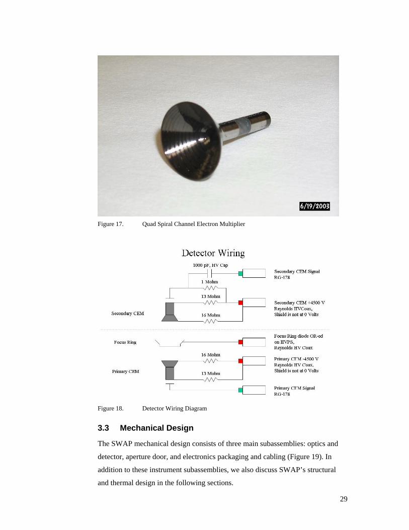
specific arrival order is required by the electronics. The CEMs have quad spiral

28

channels with a resistance of 300 Mohm and dark counts less than 40 mHz

(Figure 17).

The coincidence detector system reduces the background from CEM dark counts

and UV noise, allowing SWAP to have a low enough noise floor to measure

heliospheric pick-up ions. Two detectors provide the redundancy needed for a

long-duration mission. SWAP can still make its primary science measurement

using only one of its CEMs. This requirement for redundancy drove us to add a

-1 kV Focus Ring supply that is slaved to the SCEM and diode OR-ed with the

PCEM supply to the Focus Ring. If the PCEM is turned off, the -1 kV Focus

Ring supply will accelerate back-scattered electrons from the carbon foil into the

SCEM.

The long CEM lifetime needed for this mission required us to select all materials

near the detector to be ultra-low outgassing. We used only glass, metal, and

ceramic materials for all parts of the detector that had venting access to the CEM

detectors. HV and LV cabling was brought to bulkheads, and the signals were

conducted through ceramic feed-thrus to the exact location they were required

(Figure 18).

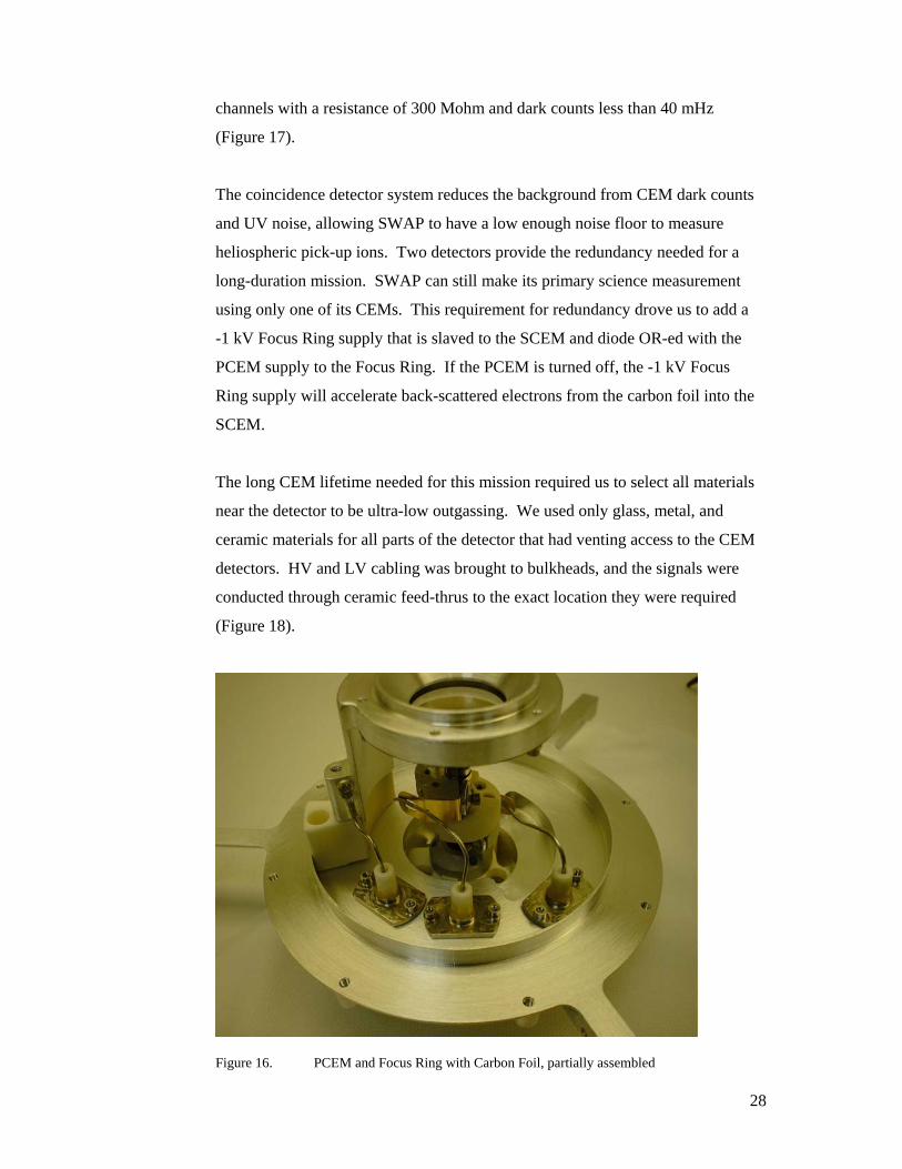
Figure 16. PCEM and Focus Ring with Carbon Foil, partially assembled

29

Figure 17. Quad Spiral Channel Electron Multiplier

Figure 18. Detector Wiring Diagram

3.3 Mechanical Design

The SWAP mechanical design consists of three main subassemblies: optics and

detector, aperture door, and electronics packaging and cabling (Figure 19). In

addition to these instrument subassemblies, we also discuss SWAP’s structural

and thermal design in the following sections.

30

Figure 19. Photograph of SWAP instrument highlighting subassemblies

3.3.1 Optics and detector mechanical design

The critical requirements driving the optics and detector mechanical design were

to mount the electro-optical components as specified by the ray-traced model,

produce optically black surfaces inside the instrument, ensure contamination

control for the detectors, provide for easy refurbishment, and accurately align all

critical components.

We used a SIMION ray tracing model to define the electro-optics component

(Figure 20) sizes and locations (RPA, ESA, CEMs), and required that the

mounting of the various elements should minimally impact particle trajectories.

We accommodated this by mounting the Inner ESA and Primary CEM assemblies

from a cantilevered support hidden in the 90° region where SWAP does not

require particle viewing. The location of this cantilever matches up with the hinge

assembly on the door.

Aperture Door Electronics Packaging

Optics and Detector

31

Figure 20. Mechanical configuration of the optics and detector assembly.

In order to accommodate the cleanliness requirement, the optics and detector areas

included a split between ultra-clean and electronics volumes. We used ceramic

for the electronics near the primary CEM, and fed the cabling into the primary

CEM area using pass-thrus in the cantilever support so that it would not pass

through the ESA gap.

We refurbished SWAP after spacecraft environmental testing, replacing the CEMs

and the ultra-thin carbon foil with ones that had been stored in a clean

environment after burn-in. To minimize the risk of dismantling the instrument,

the CEM assemblies were designed so that they could be easily replaced. In order

to meet the alignment requirements for the electro-optics, we designed features

that would control the concentricity and placement of the optics and detectors in

relation to each other both before and after refurbishment.

3.3.2 Aperture door design

The aperture door’s (Figure 21) main requirement is to protect the SWAP RPA

from contamination and damage during ground and launch operations. Although

we designed the door to open one time at launch, it was important that it easily

reset for test on the spacecraft. We opened the door multiple times as part of the

RPA

Outer ESA Inner ESA

Primary CEM

Secondary CEM Top-hat

32

instrument verification and during the environmental test flow at the spacecraft

level. The door could not be a glinting source because it stays with SWAP during

the entire mission to Pluto. Spacecraft requirements dictated that external surfaces

be conductively coupled to the instrument. Therefore, we coated the door surfaces

with black nickel and provided for ground straps built into the design. The New

Horizons Component Environmental Specification required verifying through test

that the door’s torque margin was greater than 2.25. Testing demonstrated a

torque margin of 3.10, and the door successfully opened in flight.

Figure 21. Door assembled on the SWAP outer ESA

3.3.3 Electronics packaging and cabling design

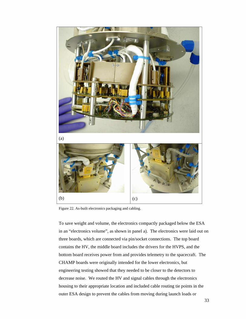
Figure 22 shows the as-built electronics packaging and cabling that are part of the

SWAP instrument. Panel a) shows the HVPS and Control board with the

electronics before the electronics housing was installed. Panels b) and c) show

different views of the CHAMP electronics and cables that brought the HV to the

RPA and ESA.

Hinge Assembly Door Frame and Door

TiNi Pinpuller

RPA

33

(a)

(b)

(c)

Figure 22. As-built electronics packaging and cabling.

To save weight and volume, the electronics compactly packaged below the ESA

in an “electronics volume”, as shown in panel a). The electronics were laid out on

three boards, which are connected via pin/socket connections. The top board

contains the HV, the middle board includes the drivers for the HVPS, and the

bottom board receives power from and provides telemetry to the spacecraft. The

CHAMP boards were originally intended for the lower electronics, but

engineering testing showed that they needed to be closer to the detectors to

decrease noise. We routed the HV and signal cables through the electronics

housing to their appropriate location and included cable routing tie points in the

outer ESA design to prevent the cables from moving during launch loads or

34

transportation. The standoffs between the three bottom boards structurally

attached the boards to the housing and allowed heat to conductively pass to the

housing.

3.3.4 Structural Design

The Component Environmental Specification defined the following critical

structural requirements for SWAP: 1) quasi-static load of 30 gs applied separately

along 3 orthogonal axes, 2) first mode structural frequency constraints of >70 Hz

(thrust direction) and (>50 Hz) (lateral direction), 3) sine vibration up to 20 g (22-

24 Hz, and 4) Random vibration with an overall amplitude of 10.4 Grms.

We performed a structural analysis during the final design phase to very that the

SWAP structure would meet these requirements. The analysis focused on the

critical items such as the cantilevered ESA and outer ESA. The analysis also

showed that the first natural frequency of the SWAP instrument, 180 Hz, was well

within the requirement. Finally, we performed vibration testing during

environmental testing to ensure that SWAP would survive the prescribed levels.

3.3.5 Thermal design

SWAP has flight temperature limits of 0 to +40°C (operating) and -20 to +50°C

(non-operating). We initially performed a thermal analysis to show that the

electronics and other temperature-sensitive parts of the SWAP instrument could

survive these temperature extremes. The analysis also showed that the heat

exchange with the spacecraft was less than 5 Watts (the limiting case was when

the instrument was at its hot limit with the door open), as required by the

spacecraft. During environmental testing, we performed a thermal vacuum test to

validate the functionality of SWAP at all temperatures within these extremes; hot

and cold turn-ons of the instrument were also performed.

3.4 Electronics

3.4.1 CHAMPs

The CHAMPs for SWAP convert a charge pulse from the CEMs into a TTL pulse

that can be registered and processed on the Control Board. The CHAMPs (Figure

35

23) are located as close to the detectors as practical in separate enclosures

mounted to the top of the strong back. The SWAP design incorporates high-speed

commercial hybrid CHAMPs, which work reliably to >1 MHz rates and have

voltage-adjustable thresholds. The output from the CEMs is brought to the

CHAMP through a short coaxial cable through a bulkhead SMA connector that

ties the shield to chassis ground. A 100-ohm resistor and back-to-back diodes

protect the input from discharges, and the input is AC coupled to the charge amp.

Injecting test pulses into the front end demonstrates the end-to-end integrity of the

microcircuits and cabling for CEM pulse processing. Test pulses are driven from

the Control Board to the CHAMP using an ACMOS level signal, which is twisted

with a return line. On the CHAMP, the signal is buffered by a gate with Schmitt

triggering.

The threshold voltage for the CHAMP is set by a Digital-to-Analog Converter

(DAC) on the Control Board, and this value can be set through standard software

commands, allowing the threshold to be updated at any time. A resistor sets the

output pulse width to 70 ns and the amplifier dead-time to 100 ns. The output

pulses from the amplifier are buffered by two Schmitt trigger buffers and

transmitted through a back-terminated series resistor to the cable that connects to

the Control Board.

Figure 23. Charge Amplifier Photograph

36

3.4.2 HVPS

The HVPS (Figure 24) set the voltages on the optical surfaces (RPA, DFL, ESA,

& Focus Ring) as well as supplying power to the Primary and Secondary Channel

Electron Multipliers (PCEM and SCEM). Table III shows the primary HVPS

properties. The two detector supplies are single string, but the two independent

detectors provide redundancy. The Focus Ring is diode-ORed with the output of

the PCEM and a -1000 V Focus Ring supply that is created and controlled in

parallel with the SCEM. The optical power supplies are redundant and diode-

ORed together. The secondary ground on the HVPS is “zap-trapped” to chassis

through back-to-back diodes for protection. Mechanically, the HVPS are built

onto two interconnected boards: the Driver Board and the Multiplier Board.

Table III. Key HVPS Specifications.

PCEM SCEM Focus Ring RPA DFL ESA Voltage Range [V]

0 to -4500 0 to +4500 0 to -1000 0 to +2000 0 to +4000 0 to -4000

Ripple 0.5 Vrms 0.5 Vrms 10 Vrms 0.1 Vrms 0.5 Vrms 0.5 Vrms Settling Time

N/A N/A N/A 100 ms to 0.1%

100 ms to 0.1%

100 ms to 0.1%

Accuracy 5 V 5 V 20% 0.5 V 4 V 4 V

Figure 24. HVPS being assembled into the SWAP sensor

37

3.4.3 Control Board

The SWAP Control Board provides the electrical interface between the New

Horizons spacecraft and the SWAP instrument. All command, telemetry, power,

safe/arm, and actuation interfaces reside on the Control Board. Software on an

8051 microcontroller responds to commands, controls the operation of the

instrument, sequences the high voltage power supplies, collects the data, and

formats telemetry for down-link.

SWAP communicates to the spacecraft through two redundant (A & B side)

asynchronous RS-422 interfaces. SWAP accepts serial commands, produces

serial telemetry, and synchronizes communication with the spacecraft through a

Pulse Per Second (PPS) line. The command and telemetry data are transmitted at

38,400 Baud.

The Control Board contains the EMI filters and DC-DC converters, which create

the +5 and -5 Volt secondary power rails that are isolated from the spacecraft

primary bus. Two separate 1.5W DC-DC Converter provide power for the

instrument. Since the DC-DC converters do not have provisions for

synchronization, each converter has an independent EMI filter to eliminate low-

frequency noise from the beat between the two converter oscillators. The Control

Board has a set of power MOSFETs, which allow us to switch low voltage power

to the PCEM HVPS, SCEM HVPS, Optical HVPS Bank A, Optical HVPS Bank

B, and the Housekeeping circuits.

The micro-controller provides all of the on-board processing required to operate

the instrument, responds to commands, and produces telemetry. The CPU

executes at 4.9152 MHz, and a minimum of 12 clocks are required to execute a

single instruction, so the top speed of the processor is 0.4 MIPS. From this low

rate, the clock can be divided down further to reduce the instruction rate to 0.05

MIPS. Due to spacecraft-level power constraints every effort was made to reduce

the operating power required for SWAP. This maximized our ability to remain on

during the Pluto encounter sequence when the spacecraft is power-limited and

only runs two optical instruments at a time.

38

Boot code for the micro-controller resides in a radiation hardened 32k x 8-bit

Programmable Read-Only Memory (PROM). This ensures that the instrument

can always boot and establish basic communication with the spacecraft even if

other memory devices have endured temporary upsets or even permanent

degradation. Two separate 128k x 8-bit Electrically Erase-able Programmable

Read-Only Memory (EEPROM) devices provide redundant storage for a 64k x 8-

bit storage area for program code an a 64k x 8-bit storage area for Look-Up

Tables (LUTs). Finally, a 128k x 8-bit Static Random Access Memory (SRAM)

is used to provide 64k x 8 bits of code memory and 64k x 8 bits of data memory.

During normal operations, if the program code in one of the EEPROM banks has

a valid checksum, then it is loaded into RAM by the Boot PROM and executed.

A Field-Programmable Gate Array (FPGA) controls the memory mapping and

memory windows that the micro-controller needs to access these devices.

Signals received from the primary and secondary CHAMPs are processed on the

Control Board. When the electro-optics have been set to the appropriate levels

and sufficient settling time has elapsed, the software opens up an acquisition

window and totals all of the primary and secondary CEM pulses that occur during

the acquisition window. Whenever a secondary or primary event occurs, a 100 ns

coincidence window is started. If a pulse is received from the other charge

amplifier during the 100 ns coincidence window, then a coincidence counter is

incremented. Due to the electro-optic design, primary and secondary events can

be received in either order. There is no dedicated start or stop channel.

The Control Board sets the RPA, DFL, and ESA high voltage optical settings

using a set of independent digital-to-analog converters (DAC). The analog

settings, along with digital enables, and the low voltage power for the primary and

redundant supplies are carried to the HVPS over a dedicated board-to-board

connector. The HVPS returns the analog current and voltage monitors to the

Control Board for analog housekeeping and real-time monitoring.

The health and safety of the instrument in general and the CEMs in particular are

monitored extensively by the Control Board. The count rate of each detector is

totaled and checked against a software limit every 0.5 s. The supply voltage and

39

strip current for each CEM is monitored and verified by the software every 1 s.

The strip current is also compared against a threshold level with 32 values. If the

strip current exceeds this threshold, the software receives an interrupt and may

immediately take action. This information, along with temperatures in the

instrument and the current and voltage monitors of the low voltage power supplies

are transmitted to the ground in housekeeping telemetry packets.

3.5 Modes of Operation

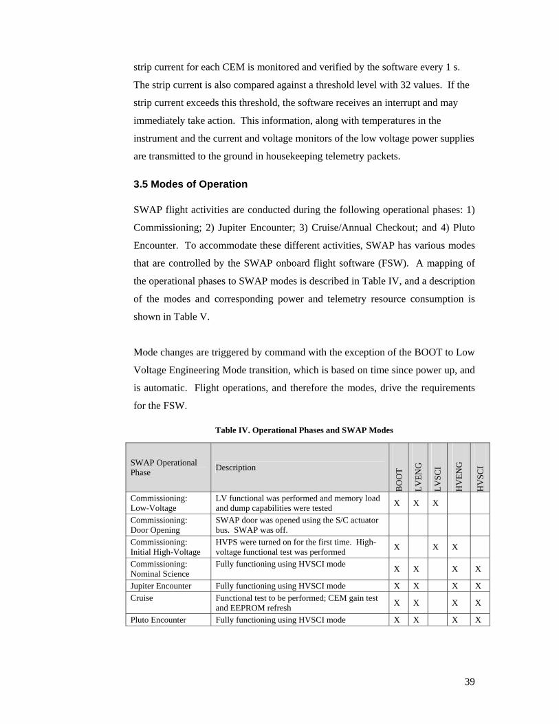
SWAP flight activities are conducted during the following operational phases: 1)

Commissioning; 2) Jupiter Encounter; 3) Cruise/Annual Checkout; and 4) Pluto

Encounter. To accommodate these different activities, SWAP has various modes

that are controlled by the SWAP onboard flight software (FSW). A mapping of

the operational phases to SWAP modes is described in Table IV, and a description

of the modes and corresponding power and telemetry resource consumption is

shown in Table V.

Mode changes are triggered by command with the exception of the BOOT to Low

Voltage Engineering Mode transition, which is based on time since power up, and

is automatic. Flight operations, and therefore the modes, drive the requirements

for the FSW.

Table IV. Operational Phases and SWAP Modes

SWAP Operational Phase Description

BO

OT

LVEN

G

LVSC

I

HV

ENG

HV

SCI

Commissioning: Low-Voltage

LV functional was performed and memory load and dump capabilities were tested X X X

Commissioning: Door Opening

SWAP door was opened using the S/C actuator bus. SWAP was off.

Commissioning: Initial High-Voltage

HVPS were turned on for the first time. High-voltage functional test was performed X X X

Commissioning: Nominal Science

Fully functioning using HVSCI mode X X X X

Jupiter Encounter Fully functioning using HVSCI mode X X X X Cruise Functional test to be performed; CEM gain test

and EEPROM refresh X X X X

Pluto Encounter Fully functioning using HVSCI mode X X X X

40

Table V. SWAP Modes and Resources

Name Description +30V S/C Power (W)

SWAP Internal (+5V/-5V) Power (W)

Telemetry Output 1 (bits/sec)

OFF No power being applied to SWAP 0 0 0

BOOT

Bootup run from PROM image. Checksum of non-volatile area and read/write tests of RAM performed. This mode has the ability to upload and commit new code and table images to EEPROM. Transition to LVENG is automatic based on time since power up.

0.70 0.44 1200

LVENG

Low-Voltage Engineering run from EEPROM image. Safe mode (no HV), no sweeping takes place, for engineering and testing

0.70 0.44 600

LVSCI

Low-Voltage Science run from EEPROM image. The instrument will begin sending test pulses through the CHAMPs in a pattern that will simulate a normal science sweep. This mode emulates HVSCI without HV.

0.74 0.48 291

HVENG

High-Voltage Engineering run from EEPROM image. HV can be set according to commands rather than being controlled by the sweep algorithm; used during initial turn-on, calibration and ramping of HVPS prior to nominal science use in HVSCI mode.

1.33 0.98 290

HVSCI High-Voltage Science run from EEPROM image. HV is on; ESA/RPA/DFL supplies are swept according to tables

1.33 0.93 (avg) 291

1 These are typical values for these modes. Other rates can be commanded as needed.

3.6 Flight Software

3.6.1 Overall Capabilities

The FSW runs on the 80C51 microprocessor at 4.9152 MHz, equating to

approximately 400,000 instructions per second. It is written almost entirely in the

C programming language. The FSW consists of two different code images stored

in nonvolatile memory. At power on, the FSW runs directly from a

programmable, read-only memory (PROM) code image. This code gathers

diagnostic information on the SWAP hardware, provides the ability to reload

EEPROM code or tables and determines which copies of EEPROM code or table

41

to use for science acquisition. Once the EEPROM code and tables have been

chosen, the EEPROM code is copied into RAM for execution.

The FSW addresses these requirements areas: data interfacing and

synchronization with the spacecraft, instrument engineering and safety, and

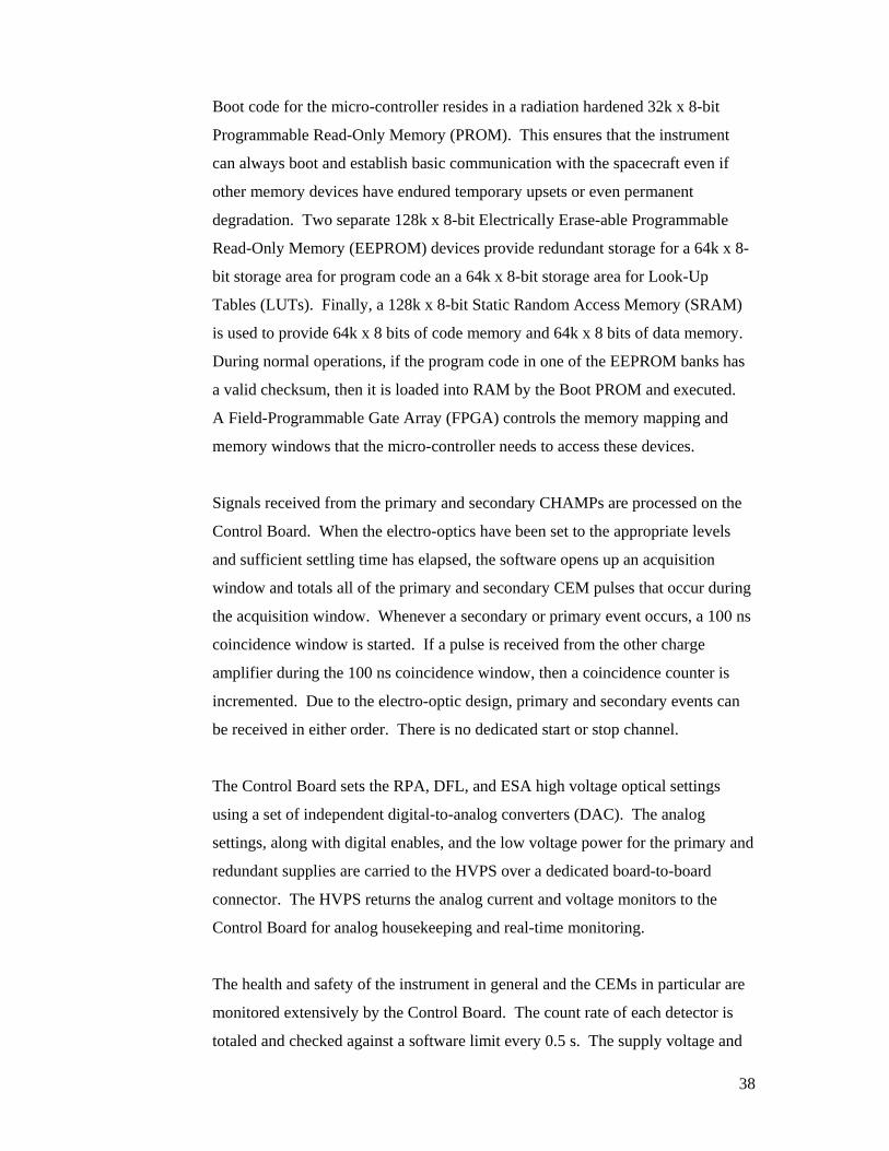
science support. The software has a fundamental cadence of 1 second

synchronized with the 1 pulse-per-second (1PPS) signal from the spacecraft. The

spacecraft sends a mission-elapsed time (MET) to each of the instruments for a

common time tag. The one-second period is subdivided into twenty 50-ms time

periods – as shown in Figure 25– which allow for scheduling of software

processes. The processes can be mapped to modes by using the legend beneath

the timeline; e.g., HVSCI mode encompasses the processes that are “Common”,

“Science Acquisition”, “HV Checking, “Science Calculation” and “HV

Sweeping.”

The relative timing of the science processes is shown in the bottom section of the

timeline. The science processes handle 1) managing the setting of HVPS levels

during science-data acquisition (during HVSCI mode, the ESA, RPA and DFL are

set by means of lookup tables), 2) starting and collecting of counter data from the

PCEM, SCEM, and coincidence electronics, and 3) performing calculations

onboard using the counter data and telemeter science-data products.

Spacecraft commands (in addition to the spacecraft MET message) to SWAP can

be sent at a rate of up to 1 per second, with the command being processed at time

= 950 ms by the “ProcessCmdBuffer” software routine. In nominal operations,

commands are required for the high-voltage ramp after a power on, but once the

ramp has been completed, six commands are used for initiating science

acquisition: 1) plan number setting, 2) angle setting, 3-6) telemetry-rate setting for

each of the housekeeping, real-time science, summary-science, and histogram-

science packets.

42

Figure 25. SWAP FSW one-second timeline showing software processes as a function of time.

The horizontal groupings show major categories with the “Spacecraft Requirements” at the top and

“Science Processes” at the bottom of the figure.

The FSW outputs three types of telemetry: instrument state information (no

APID) which can be read and acted upon by the spacecraft software for onboard

anomaly recovery; CCSDS engineering telemetry (housekeeping, messages and

memory dump); and CCSDS science telemetry (real-time, summary and

histograms). The CCSDS-level data are processed in the Level 1 Data Pipeline.

The telemetry is summarized in Table VI.

43

Table VI. SWAP Telemetry

Name APID Description Typical Packet Rate

Typical Bit Rate (bps)

Instrument State

N/A SWAP information used onboard by S/C autonomy software. Instrument state includes heartbeat and safety flags.

1 Hz Varies – not considered part of SWAP

Housekeeping (Engineering)

0x580 Instrument status are contained in this packet (e.g., opcode echo, FPGA status, non-safety-critical monitors, software variable status, etc.)

0.5 Hz in LVENG; once every 64 seconds in other modes

292 in LVENG; 9.1 in other modes

Memory Dump (Engineering)

0x581 Memory dump for diagnostics Low N/A

Message (Engineering)

0x582 Warning message that is issued to provide additional detail if anomalous activities occur.

Low N/A

Real-time (Science)

0x584 Contains the most detailed temporal data from SWAP consisting of RPA, ESA and DFL commanded DAC levels corresponding primary CEM, secondary CEM and coincidence counts.

1 Hz during commissioning; 1 set of 64 consecutive packets per hour otherwise

280 during commissioning and Pluto Encounter; 5.0 otherwise

Summary (Science)

0x585 Summary accumulation over a set period of time, typically an hour. A calculation is performed using the coincidence data from the previous 64-second period to generate values that are related to density, velocity and temperature and output in telemetry. The minimum, maximum and variance of these parameters are also output in telemetry.

1 per hour 0.19

Histogram (Science)

0x586, 0x587

All of the count data are accumulated over a set period of time, typically a day. The data are accumulated in a normalized energy array of 2048 elements. The normalization occurs such that for each 64-second acquisition period, the center of the array corresponds to the solar wind peak during those 64 seconds. The entire array is brought down in telemetry. Because of its size, the array must be trickled out in 64 packets. This packet contains the histogram header (APID 0x586) and the beginning of the histogram data. It is followed by 63 Science Histogram Data (APID 0x587) packets to create a complete histogram set.

1 set of 64 (1 header + 63 data) packets per day

0.15

3.6.2 Science-Data Collection

Science data are collected in the HVENG and HVSCI modes. HVENG was used

extensively during commissioning for initial HV ramp-up and instrument

44

response characterization; however, HVSCI is the primary SWAP science mode.

In HVSCI, the optical power supplies are stepped every 0.5 seconds and the

PCEM, SCEM and coincidence counter data are collected with each step. An

overall cadence of 64 seconds consisting of 128 0.5-second steps defines the 64-

second science-acquisition frames and hence all science FSW activities. A typical

64-second frame consists of a 32-second coarse sweep, which covers the entire

energy range with 64 logarithmically-spaced steps in energy, followed by a 32-

second (also 64 0.5-second steps) fine sweep. The peak value of the coincidence

counter during the coarse sweep is calculated to determine the center of the fine

sweep so that finer resolution sweeping around the peak response can be

performed. The counter sample duration of 390 milliseconds for every 0.5-second

step allows for power supply settling time.

A 64-second acquisition frame period from SWAP calibration is shown in Figure

26. It shows the PCEM, SCEM and coincidence count rates, and the ESA and

RPA voltages. In this experiment, DFL was set to 0 throughout this data set since

the angle relative to the SWAP aperture was 0°. The figure shows that for SWAP,

the energy is swept from high to low, with the coarse sweep taking place from

time = 0 to 32 seconds and a fine sweep from time = 32 to 64 seconds.

Figure 26. A coarse and fine sweep acquired during SWAP ground calibration activities.

45

To control the sweeping, acquisition and processing of science data, SWAP has

two identical copies of lookup table sets stored in separate EEPROMs. Each copy

consists of:

• 64 plans of 32 plan steps

• 16 sweeps of 128, 0.5-second steps

• ESA based on sweep types (coarse, fine, others) x 1024 energy settings

• DFL based on 256 energy (reduced energy resolution by a factor of 4 from

1024) x 32 angles

• RPA based on 4 sweep types x 1024 energy settings

• RPA angle adjust based on 512 energy (reduced energy resolution by a

factor of 2 from 1024) x 32 angles

Figure 27 illustrates the use of the tables. The plan table, (“X” was commanded

in the figure example) which acts as the overall “script”, is accessed only at the

beginning of a 64-second acquisition period. It contains the sweep table number

(“A”) and number of repetitions of frames to execute that sweep table

consecutively before moving to the next step in the plan. If the number of frames

is 0, then the plan restarts at plan step 0.

The sweep table chosen is based on the sweep table number from the plan table.

The same sweep table is used throughout the 64-second frame. The sweep table is

accessed every 0.5 seconds so that each of the 128 steps can be controlled

throughout the frame. The sweep table outputs the ESA-RPA table number (“B”

for the first 32 seconds and “C” for the second 32 seconds), which would

correspond to coarse, fine, and others; the index type (absolute used for coarse

sweeping or relative used for fine sweeping) and the energy index, a number from

0 to 1023 which corresponds to a particular energy setting throughout all the ESA,

DFL, RPA and RPA angle adjust tables. Energy index is labeled “E-Index” in the

figure. If the index type is absolute, then the energy index is used, as-is from the

sweep table. Typically, to cover the entire energy range in 64 coarse sweep steps,

every 16th entry of the 1024-element table is chosen. If relative, then the E-index

in the table is an offset used to align the energy index associated with the

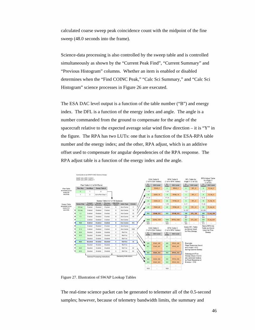
46

calculated coarse sweep peak coincidence count with the midpoint of the fine

sweep (48.0 seconds into the frame).

Science-data processing is also controlled by the sweep table and is controlled

simultaneously as shown by the “Current Peak Find”, “Current Summary” and

“Previous Histogram” columns. Whether an item is enabled or disabled

determines when the “Find COINC Peak,” “Calc Sci Summary,” and “Calc Sci

Histogram” science processes in Figure 26 are executed.

The ESA DAC level output is a function of the table number (“B”) and energy

index. The DFL is a function of the energy index and angle. The angle is a

number commanded from the ground to compensate for the angle of the

spacecraft relative to the expected average solar wind flow direction – it is “Y” in

the figure. The RPA has two LUTs: one that is a function of the ESA-RPA table

number and the energy index; and the other, RPA adjust, which is an additive

offset used to compensate for angular dependencies of the RPA response. The

RPA adjust table is a function of the energy index and the angle.

Figure 27. Illustration of SWAP Lookup Tables

The real-time science packet can be generated to telemeter all of the 0.5-second

samples; however, because of telemetry bandwidth limits, the summary and

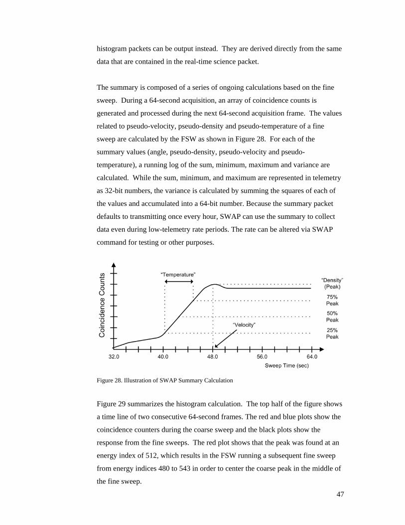
47

histogram packets can be output instead. They are derived directly from the same

data that are contained in the real-time science packet.

The summary is composed of a series of ongoing calculations based on the fine

sweep. During a 64-second acquisition, an array of coincidence counts is

generated and processed during the next 64-second acquisition frame. The values

related to pseudo-velocity, pseudo-density and pseudo-temperature of a fine

sweep are calculated by the FSW as shown in Figure 28. For each of the

summary values (angle, pseudo-density, pseudo-velocity and pseudo-

temperature), a running log of the sum, minimum, maximum and variance are

calculated. While the sum, minimum, and maximum are represented in telemetry

as 32-bit numbers, the variance is calculated by summing the squares of each of

the values and accumulated into a 64-bit number. Because the summary packet

defaults to transmitting once every hour, SWAP can use the summary to collect

data even during low-telemetry rate periods. The rate can be altered via SWAP

command for testing or other purposes.

Figure 28. Illustration of SWAP Summary Calculation

Figure 29 summarizes the histogram calculation. The top half of the figure shows

a time line of two consecutive 64-second frames. The red and blue plots show the

coincidence counters during the coarse sweep and the black plots show the

response from the fine sweeps. The red plot shows that the peak was found at an

energy index of 512, which results in the FSW running a subsequent fine sweep

from energy indices 480 to 543 in order to center the coarse peak in the middle of

the fine sweep.

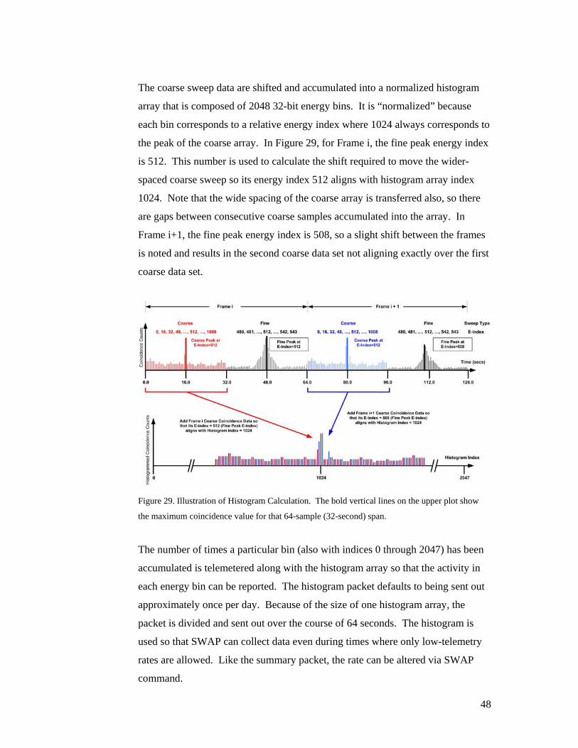
48

The coarse sweep data are shifted and accumulated into a normalized histogram

array that is composed of 2048 32-bit energy bins. It is “normalized” because

each bin corresponds to a relative energy index where 1024 always corresponds to

the peak of the coarse array. In Figure 29, for Frame i, the fine peak energy index

is 512. This number is used to calculate the shift required to move the wider-

spaced coarse sweep so its energy index 512 aligns with histogram array index

1024. Note that the wide spacing of the coarse array is transferred also, so there

are gaps between consecutive coarse samples accumulated into the array. In

Frame i+1, the fine peak energy index is 508, so a slight shift between the frames

is noted and results in the second coarse data set not aligning exactly over the first

coarse data set.

Figure 29. Illustration of Histogram Calculation. The bold vertical lines on the upper plot show

the maximum coincidence value for that 64-sample (32-second) span.

The number of times a particular bin (also with indices 0 through 2047) has been

accumulated is telemetered along with the histogram array so that the activity in

each energy bin can be reported. The histogram packet defaults to being sent out

approximately once per day. Because of the size of one histogram array, the

packet is divided and sent out over the course of 64 seconds. The histogram is

used so that SWAP can collect data even during times where only low-telemetry

rates are allowed. Like the summary packet, the rate can be altered via SWAP

command.

49

4.0 Instrument Performance

We characterized SWAP’s performance through both laboratory testing and

electro-optics modeling. The purpose of the laboratory testing was to calibrate the

instrument and determine a ground truth. The computer models allowed us to

examine more combinations of incident-beam and instrument parameters than

possible in laboratory testing and to allow for analysis of other parameter

combinations as needed after launch.

4.1 Laboratory Testing

SWAP was extensively calibrated at the SwRI Ion Calibration Facility. This

facility produces ion beams from <500 eV to 51 keV. The ion species can be

selected for mass per charge from 1 to >40. Figure 30 shows the SWAP

instrument mounted on the facility’s 4-axis positioning system, with the doors that

protect the sensor for launch in their open configuration. Full functionality of the

instrument was demonstrated during calibration, including its ability to open the

doors while under high vacuum. The four-axis positioning system allows vertical

and horizontal displacement in the plane normal to the ion bean and rotation about

two orthogonal axes that cross in the beam path: the outer rotation is about a

vertical axis, and the inner, nested, rotation about a horizontal axis.

Figure 30. SWAP instrument mounted on 4-axis positioning system

50

The SWAP instrument was mounted with its center axis aligned to the inner-stage

rotation axis, which is equivalent to roll maneuvers the New Horizons spacecraft

will perform. Because of SWAP’s 17-cm diameter aperture, outer-stage rotations

resulted in translation in the input aperture. We used the horizontal stage to return

the aperture to its original position. The positioning system’s range of motion is

large enough to fully illuminate the instrument’s FOV.

In addition to testing performed on individual components and on a high-fidelity

prototype, the full flight instrument underwent a number of calibrations.

Calibrations were performed before and after instrument level environmental

testing, after refurbishment activities following spacecraft environmental testing

and a limited engineering beam test immediately prior to delivery to the spacecraft

for final integration. The instrument was calibrated over the full angular response

and energies from 500 eV to 8 keV. Due to the nature of electrostatic optics, the

response of the instrument to other energies can be easily scaled. Because the

solar wind protons have a nominal energy of ~1 keV, a large fraction of the

calibration data was taken at this energy. Results presented here are from the

instrument in the final delivered configuration.

4.1.1 RPA

Figure 31 shows the measured energy response of the RPA to a beam of 1 keV

protons. The primary, secondary, and coincidence rates are shown in blue, green

and orange, respectively. The RPA grids are curved, rounding the cutoff of the

transmission as compared to a planer RPA. This is seen as the reduction of counts

from 950 V to 1000 V. However, as shown in Figure 10, above, by making small

steps in the RPA voltage, we are able to differentiate beams that are only ~1-2 eV

apart at 1 keV.

51

Figu

re 31. Measured energy response of RPA to a beam of 1 keV protons

Figure 32 shows the general shape of the RPA response over the full voltage

range. Normalized coincidence is plotted as a function of the RPA voltage/beam

energy. Because the individual RPA grids have a finite thickness, they act as a

series of electrostatic lenses. The features in this figure, including maximum near

945 V, are due to the focusing properties, as discussed below in Section 4.2.

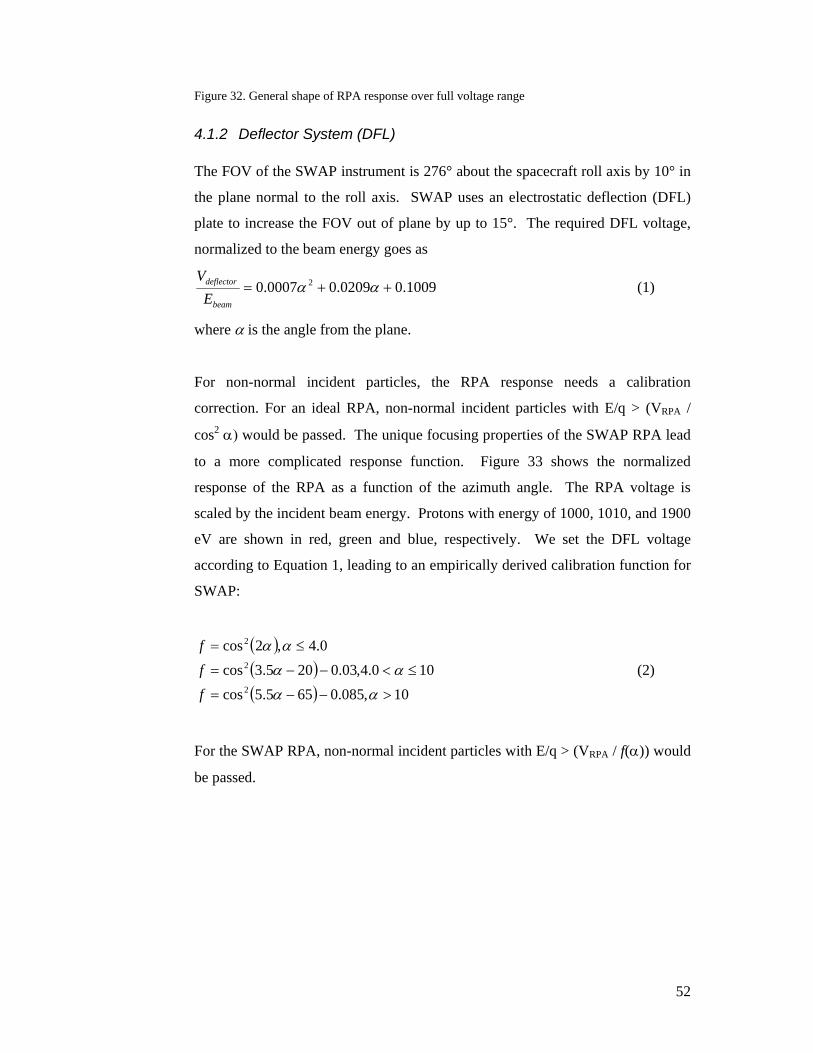
52

Figure 32. General shape of RPA response over full voltage range

4.1.2 Deflector System (DFL)

The FOV of the SWAP instrument is 276° about the spacecraft roll axis by 10° in

the plane normal to the roll axis. SWAP uses an electrostatic deflection (DFL)

plate to increase the FOV out of plane by up to 15°. The required DFL voltage,

normalized to the beam energy goes as

1009.00209.00007.0 2 ++= ααbeam

deflector

EV

(1)

where α is the angle from the plane.

For non-normal incident particles, the RPA response needs a calibration

correction. For an ideal RPA, non-normal incident particles with E/q > (VRPA /

cos2 α) would be passed. The unique focusing properties of the SWAP RPA lead

to a more complicated response function. Figure 33 shows the normalized

response of the RPA as a function of the azimuth angle. The RPA voltage is

scaled by the incident beam energy. Protons with energy of 1000, 1010, and 1900

eV are shown in red, green and blue, respectively. We set the DFL voltage

according to Equation 1, leading to an empirically derived calibration function for

SWAP:

( )( )( ) 10,085.0655.5cos

100.4,03.0205.3cos0.4,2cos

2

2

2

>−−=

≤<−−=

≤=

αα

αα

αα

fff

(2)

For the SWAP RPA, non-normal incident particles with E/q > (VRPA / f(α)) would

be passed.

53

0.75

0.8

0.85

0.9

0.95

1

0 2 4 6 8 10 12 14 16

1000eV1010eV1900eV

Azimuth Angle

Norm

aliz

ed

RP

AV

oltage

Figure 33. Normalized response of RPA as a function of azimuth angle

4.1.3 ESA

Figure 34 shows an example of the energy-angle response of the ESA to a 1keV

proton beam. The RPA and deflector system’s voltages were at zero for the data

shown here. For this ESA, the analyzer constant is 1.88, the energy resolution

∆E/E is 8.5%, and the angular FOV, undeflected, is 10°.

Figure 34. Example of calibration data

In addition to performing the coarse energy measurement, the ESA also blocks

out UV light to the detectors. A Krypton line source, with emission at 123.6 nm

and approximately the same intensity of the Sun at 1 AU, was used to test SWAP

for light leaks. We used this worst-case test since SWAP operates further out in

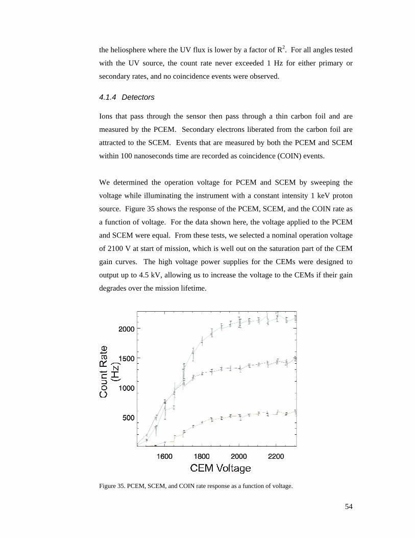
54

the heliosphere where the UV flux is lower by a factor of R2. For all angles tested

with the UV source, the count rate never exceeded 1 Hz for either primary or

secondary rates, and no coincidence events were observed.

4.1.4 Detectors

Ions that pass through the sensor then pass through a thin carbon foil and are

measured by the PCEM. Secondary electrons liberated from the carbon foil are

attracted to the SCEM. Events that are measured by both the PCEM and SCEM

within 100 nanoseconds time are recorded as coincidence (COIN) events.

We determined the operation voltage for PCEM and SCEM by sweeping the

voltage while illuminating the instrument with a constant intensity 1 keV proton

source. Figure 35 shows the response of the PCEM, SCEM, and the COIN rate as

a function of voltage. For the data shown here, the voltage applied to the PCEM

and SCEM were equal. From these tests, we selected a nominal operation voltage

of 2100 V at start of mission, which is well out on the saturation part of the CEM

gain curves. The high voltage power supplies for the CEMs were designed to

output up to 4.5 kV, allowing us to increase the voltage to the CEMs if their gain

degrades over the mission lifetime.

Figure 35. PCEM, SCEM, and COIN rate response as a function of voltage.

55

4.2 Instrument Modeling

We obtained instrument-modeling results with ion-optics simulations using

SIMION 7.0 software (Dahl, 2000). SIMION is an ion-optics simulation program

that models problems with 2D or 3D electrostatic potential arrays. It creates

potential arrays based on a user-given geometry input (usually in the form of a

text file containing commands). The potentials of points outside the electrodes are

determined by solving the Laplace equation by finite difference methods with a

maximum of 50-million array elements. The time-step integration for the

calculation of ion trajectories uses a fourth-order Runge-Kutta method, with ions

flown individually or in groups. Parameters such as position, velocity

components, energy, etc. can be recorded at different locations in the instrument

model.

The SWAP model consists of a 3D geometry with cylindrical symmetry. The

limitation of 50-million array elements prevents reproducing the finer structure of

the RPA design with the instrument design in the same potential array. Therefore,

the RPA grids are modeled separately with a much finer resolution. We discuss

the SWAP model (instrument with “ideal” RPA) in Section 4.2.1, and describe the

RPA model in Section 4.2.2.

4.2.1 Instrument Model with Ideal RPA

For the ESA electro-optics we used a 2D model cylindrical symmetry, sometimes

called 2.5D. Nevertheless, ions move in 3D space inside the model. Our model

geometry (Figure 36) fully conforms to the as-built mechanical design of the

flight instrument, with as much detail as the resolution permits. This mechanical

detail helps us account for effects such as fringing fields. The presence of doors

breaks the symmetry and is not accounted for in the model, but we can neglect the

effects on the electro-optics within the field-of-view of the instrument.

56

Figure 36. Cross section of the electro-optics model for the ESA. The model has a main axis of

symmetry.

The instrument was thoroughly characterized with ion beam calibrations (above)

and the results agree very well with those from the modeling. Table VII compares

the energy-per-charge resolution, the k factor and the angular acceptance.

Table VII. Comparison of the instrument characterization between measurements with ion beam and model

Calibration with ion beam Instrument model E/q resolution (∆EFWHM/E) 8.5 % 9.5 % * k [V/eV] 1.88 1.86 Angular acceptance at HM [°] (undeflected) -4.9 to +5.2 -4.6° to 8.1° * *Model is broader because collimating effects of RPA are not included.

Figure 37 shows the angle-energy response. The angle and energy binnings have

been intentionally set at the same values for better comparison. The right portion

of the figure shows the normalized transmission, which is color-coded using a

logarithmic scale. Again, there is excellent agreement between the modeling and

the calibration measurements with ion beam.

57

Figure 37. Comparison between the angle-energy transmission function of the instrument (left) and

the model (right).

4.2.2 RPA Model

We modeled the RPA grids separately with a much higher resolution, matching

the thickness and hole pattern of the mechanical drawings. The model includes the

curvature of the grids and drilled holes, which are perfectly aligned for the four

grids. This configuration does not account for a possible misalignment of the hole

patterns, which may cause some differences between the model and actual

hardware. Figure 38 shows an isometric view of part of the RPA.

Figure 38. Isometric view of a part of the RPA. The voltage is applied on the two middle grids.

The holes are aligned so that their axes are radial. The thickness of the grids and the diameter of

the holes are in accordance to the mechanical drawings.

58

The ions are flown through the RPA grids, and the Cartesian coordinates and

velocity-vector components are recorded at the exit of the RPA for those ions that

make it through. Those ions are then flown inside the instrument model described

in Section 4.2.1, and an ion that makes it to the carbon foil is considered to be

detected.

In the following discussion, we present results using a 1 keV/q parallel beam,

which is uniformly distributed over the aperture of the instrument at normal

incidence (0° in azimuth and elevation). Figure 39 shows a transmission curve as

a function of the RPA voltage for an ESA voltage of -524 V, with the ordinate in

arbitrary units. The red curve depicts the results of the RPA model and is

compared to the calibration data under the same conditions (black curve).

Figure 39. Relative transmission function as a function of the RPA voltage for a 1 keV/e ion beam

and an ESA voltage of –524 V.

59

The RPA does not give a sharp cut-off at 1 kV because each hole of the RPA

grids acts like a tiny lens, focusing or defocusing the ion trajectories. At a given

E/q, the deflection increases with the RPA voltage. Because of the grid thickness,

some ions hit the inside of the holes, which can also cause a non-uniform response

below the cut-off. Because the model holes are radially aligned, the energy per

charge and the RPA voltage have to be within a certain ratio for the trajectory to

deviate from a row of holes to another neighboring row. Therefore, transmission

varies as a function of RPA voltage for a particular energy per charge. Although

the general responses are similar, a discrepancy exists between the calibration data

and the simulations. The likely case of this discrepancy is that the RPA grid holes

are not aligned along a radial direction. In addition, the ion beam was entering the

instrument with a small angle with respect to the normal of the RPA grids (offset

in azimuth and/or elevation angle) and the ion beam has a small divergence (~1.0°

at 1 keV/e). These results highlight the importance of using the flight calibration

data and not simply relying on the instrument model for understanding the

detailed response function.

We presented above the simulation results for one particular case, however the

ESA, deflector, and RPA responses were simulated with numerous different initial

conditions. The model aids in understanding the instrument response and provides

additional interesting information that can be used for the analysis and

interpretation of the data.

5.0 Science Operations and Data

This section describes the expected fluxes and predicted count rates, instrument

operations, and data pipeline. We used the fluxes measured from previous

missions and the instrument model described above to estimate the anticipated

count rates in the solar wind and Jupiter. The subsequent operations discussion

describes the voltage settings, which vary according to the anticipated count rates.

Finally, the data pipeline section describes the data products and level 2 data

analysis.

60

5.1 Fluxes and Predicted Rates

We predict SWAP count rates in the solar wind scaling from fluxes observed by

Voyager 2. The proton flux decreases with distance from the Sun (Figure 40)

primarily because the density decreases with distance. For our calculations we

use a constant speed of 440 km s-1. Fit functions for the density, and density

standard deviations are listed below; the standard deviation for the speed is based

on Figure 6 of Richardson et al., (1996).

np = 5.22r−1.93 [cm−3] (3a)

σ(np ) = 7.4r−2.15 [cm−3] (3b)

We used the solar wind fluxes from Figure 40 and the instrument model described

above to estimate primary and SCEM count rates in the solar wind as a function

of heliocentric distance. The results are shown in Figure 41. The instrument model

includes the instrument effective area and the ESA and RPA response curves. The

model also includes the deflector and angular response function (FOV) and

assumes a 1 keV beam centered in the ESA passband. The red line at 1 MHz

indicates a reasonable maximum count rate for the detectors. Although the count

rates are too high in the inner heliosphere with these voltage settings, the RPA and

ESA voltages can be adjusted to reduce passband.

As described above, the ESA and RPA can be crossed to provide a reduced

energy passband. Figure 42 shows the estimated count rates as a function of the

center energy of the ESA (kVESA) passband for a 1 keV beam with a flux that is

one standard deviation higher than the average flux at 5 AU. Each curve

corresponds to sweeping the RPA and ESA voltages while keeping the RPA

voltage to ESA energy ratio fixed. At a ratio of 1.03 the expected count rates at

5AU are reduced to near maximum allowable levels, and for a ratio of 1.05 the

expected rates are <105 Hz. For the last phase of commissioning we used a ratio

of 1.05 for safety.

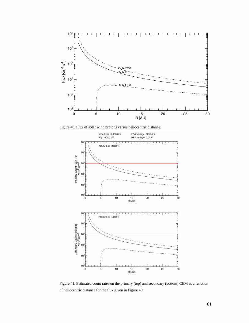
61

Figure 40. Flux of solar wind protons versus heliocentric distance.

Figure 41. Estimated count rates on the primary (top) and secondary (bottom) CEM as a function

of heliocentric distance for the flux given in Figure 40.

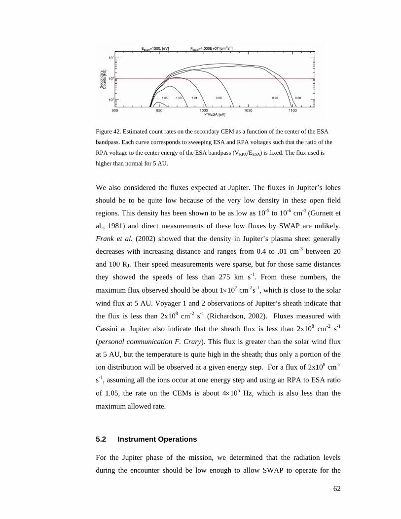
62

Figure 42. Estimated count rates on the secondary CEM as a function of the center of the ESA

bandpass. Each curve corresponds to sweeping ESA and RPA voltages such that the ratio of the

RPA voltage to the center energy of the ESA bandpass (VRPA/EESA) is fixed. The flux used is

higher than normal for 5 AU.

We also considered the fluxes expected at Jupiter. The fluxes in Jupiter’s lobes

should be to be quite low because of the very low density in these open field

regions. This density has been shown to be as low as 10-5 to 10-6 cm-3 (Gurnett et

al., 1981) and direct measurements of these low fluxes by SWAP are unlikely.

Frank et al. (2002) showed that the density in Jupiter’s plasma sheet generally

decreases with increasing distance and ranges from 0.4 to .01 cm-3 between 20

and 100 RJ. Their speed measurements were sparse, but for those same distances

they showed the speeds of less than 275 km s-1. From these numbers, the

maximum flux observed should be about 1×107 cm-2s-1, which is close to the solar

wind flux at 5 AU. Voyager 1 and 2 observations of Jupiter’s sheath indicate that

the flux is less than 2x108 cm-2 s-1 (Richardson, 2002). Fluxes measured with

Cassini at Jupiter also indicate that the sheath flux is less than 2x108 cm-2 s-1

(personal communication F. Crary). This flux is greater than the solar wind flux

at 5 AU, but the temperature is quite high in the sheath; thus only a portion of the

ion distribution will be observed at a given energy step. For a flux of 2x108 cm-2

s-1, assuming all the ions occur at one energy step and using an RPA to ESA ratio

of 1.05, the rate on the CEMs is about 4×105 Hz, which is also less than the

maximum allowed rate.

5.2 Instrument Operations

For the Jupiter phase of the mission, we determined that the radiation levels

during the encounter should be low enough to allow SWAP to operate for the

63

entire encounter. SWAP’s shielding is similar to Ulysses-SWOOPS, and the New

Horizons spacecraft does not get as close to Jupiter’s radiation belts as Ulysses

did. Phillips et al., (1993) showed that Ulysses/SWOOPS operated as close as 16

RJ, compared to the New Horizon’s closest approach is about 32 RJ. Inbound to

Jupiter, we anticipate that real-time science mode data will be taken twice per

hour, with 20 measurements recorded per hour in Jupiter’s tail. The Jupiter tail

observations continue until about 100 days after closest approach, which

corresponds to about 2200 RJ. While not designed for measuring Jovian ion

distributions, we are hopeful that some good new observations will be possible.

Past Jupiter, we plan cruise phase science with PEPPSI and REX to study how the

solar wind and pickup ions evolve with radial distance from the Sun. For cruise

phase, real-time data will be recorded at a low rate and summary and histogram

data a moderate rate. In addition, the gain on the CEMs will be measured during

each annual check out.

For the New Horizons primary mission, we will use SWAP’s maximum sensitivity

and operate at its highest rate throughout the Pluto and KBO flybys. These

observations give a spatial resolution of <3000 km, adequate to determine if Pluto

has a bow shock and if so, locate it with sufficient accuracy to make a good

measure of the atmospheric escape rate.

5.3 Data Pipeline

SWAP data are provided at three levels in the data pipeline. Level 1 is the raw

data decommuted and placed into FITS files. Level 2 involves converting the

level 1 data to more physical units, correlating data with thruster firings to look

for any enhanced backgrounds, calculating some orbital and pointing information,

and producing E/q spectrograms. For level 3, we further process the data to obtain

speed, temperature, and relative density.

5.3.1 Level 1

Level 1 data are comprised of real-time science, summary, histogram, and

housekeeping packets. We decommute and place the raw data into FITS files.

64

Most of the SWAP data consist of binary tables with columns for given

instrument parameters and rows for each measurement time. Since the histogram

data consist of arrays, it is stored as an image in the FITS file.

We place all the real-time data for a given day into one file. A complete real-time

observation consists of 64 real-time packets. In order to make sure that an

instrument cycle is not split across two daily files, a parameter in the real-time

packet is used, which indicates the beginning and end of the 64-second instrument

cycle. We also create daily files for summary data, but the histogram data are

handled differently since the histogram arrays are divided into 64 packets. A set of

64 histogram packets are combined and placed into one file.

We divide each FITS file into extensions. The first two real-time data extensions

contain header information and the real-time data as a binary table. Additional

table extensions contain housekeeping and thruster-firing data. We use this same

organization for the summary data. The first two histogram extensions contain the

array (image) with the number of samples placed into each bin, and another image

holds the array of counts detected in each bin. The housekeeping, thruster, source

sequence count (used to check for data gaps) and checksum (used to check for

corrupted data) information is contained in additional extensions. For real-time

and summary files, the source sequence and checksum information is not stored as

separate extensions, but directly inside the tables.

5.3.2 Level 2

We also store SWAP level 2 data as binary tables and images in FITS files. The

header information from level 1 is duplicated into level 2, since the header

contains level 1 processing information and orbit-attitude information for the start

time of the each file. The second extension for the real-time and summary level 2

files contains the corresponding data from those packets converted from raw to

engineering units, e.g., converting the RPA DAC step number to voltage. The

real-time files contain several additional extensions that hold spectrogram

information. These extensions consist of the coarse scan (1st 32 steps) 2D

spectrogram count arrays, the corresponding 2D error spectrograms, the y-axis

65

labels (energy label) for the spectrograms, and the x-axis time label information.

The real-time and summary files have housekeeping, quality, and thruster firing

extensions. The histogram level 2 file format mirrors histogram level 1 format, but

includes quality flags.

We base the flags that assess the quality of the data on housekeeping data, orbit

and attitude, and how well the software is working. Currently, these flags are

based on standard operating ranges for housekeeping data, but additional ones can

be created later as needed.

We are developing SPICE code to calculate the time in UTC, position and

velocity of the spacecraft in a variety of coordinate systems, field of view of the

instrument, and the Sun location in instrument coordinates. The boresight of

SWAP is nearly aligned with the +Ysc axis; therefore the SWAP frame kernel

consists of only two small rotations from spacecraft to instrument coordinates. We

are integrating SPICE code into the level 2 code, and an orbit and attitude table

extension with all SPICE calculations for each measurement time is planned for

the level 2 files. Flags will be created to indicate whether or not the Sun is

SWAP’s FOV since accurate solar wind properties can only be determined if the

bulk of the solar wind beam enters the instrument.

We will produce energy-time spectrograms from real-time science mode data.

These count rate spectrograms provide a way to examine the data at high time

resolution over the full energy range of the instrument. Such spectrograms have

proven useful for analyzing a wide variety of distribution types. They have been

used to analyze the solar wind, comets, plasma boundaries, and shocks. As an

example, Figure 43 shows a spectrogram used to analyze ion measurements for

the comet Borrelly flyby. In this figure it is easy to locate the bow shock and see

the slowing of the solar wind due to mass loading.

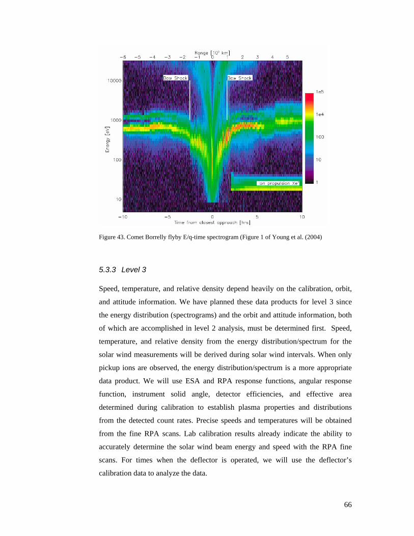
66

Figure 43. Comet Borrelly flyby E/q-time spectrogram (Figure 1 of Young et al. (2004)

5.3.3 Level 3

Speed, temperature, and relative density depend heavily on the calibration, orbit,

and attitude information. We have planned these data products for level 3 since

the energy distribution (spectrograms) and the orbit and attitude information, both

of which are accomplished in level 2 analysis, must be determined first. Speed,

temperature, and relative density from the energy distribution/spectrum for the

solar wind measurements will be derived during solar wind intervals. When only

pickup ions are observed, the energy distribution/spectrum is a more appropriate

data product. We will use ESA and RPA response functions, angular response

function, instrument solid angle, detector efficiencies, and effective area

determined during calibration to establish plasma properties and distributions

from the detected count rates. Precise speeds and temperatures will be obtained

from the fine RPA scans. Lab calibration results already indicate the ability to

accurately determine the solar wind beam energy and speed with the RPA fine

scans. For times when the deflector is operated, we will use the deflector’s

calibration data to analyze the data.

67

6.0 Conclusions

The SWAP instrument on New Horizons will provide the best measurement of the

global atmospheric escape rate from Pluto. This escape rate determines the type of

interaction that Pluto has with the solar wind. For a large escape rate, with many

ions leaving the atmosphere, the interaction should be comet-like, where

ionization of atmospheric material mass loads the solar wind, causing slowing of

the overall bulk flow of the solar wind and draping of the IMF. For lower escape

rates, the interaction is likely more like the interaction that the solar and wind has

with Venus. There, the interaction size is much smaller and the solar wind

interacts directly with ions closely bound to planetary atmosphere, causing a much

smaller region of draped magnetic field. In either case, SWAP should also be able

to identify and locate a bow shock, if one exists.

In addition to measuring the overall escape rate from Pluto’s atmosphere and

allowing us to develop an understanding of the solar wind interaction with Pluto

for the first time, SWAP should also be able to measure hydrogen pickup ions

around Pluto. In addition, in the unlikely event that Pluto has any significant

internal or remnant magnetic field, SWAP should measure the effects that such a

field would have on the solar wind plasma interaction. Finally, en route to Pluto

and Kuiper belt objects beyond, SWAP should make unique observation of the

variation of heliospheric pickup hydrogen ions and sample the Jovian

magnetosphere.

The SWAP instrument was designed to meet the unique and challenging

requirements of measuring the solar wind and its interaction with Pluto out at 30

AU, from a spacecraft that scans its orientation over large angles in order to image

Pluto and Charon with body-mounted cameras as it flies by. In addition, because

observations of the plasma interaction is not primary science for the mission,

resources for SWAP were highly constrained and we had to remain focused on

developing a simple instrument optimized only for measurements of the solar

wind interaction with Pluto, while working within the detailed constraints of the

New Horizons spacecraft and mission plan.

68

To satisfy all of these requirements and constraints, we designed the SWAP

instrument to be cylindrical symmetric over 270° of rotation angle, and combined

an RPA that acts a high pass filter, a deflector ring, and an ESA. Different

combinations of the RPA and ESA produce a variable passband and

deconvolution of measurements made while micro-stepping the RPA allows the

measurement of very small changes in the solar wind speed. Ions that pass

through the SWAP electro-optics are then measured in a coincidence detector

section that both provides redundancy for making the measurements and

suppresses the background for noise generated by anything other than real ions

transiting through the instrument. The SWAP instrument has been well

characterized by both ground calibrations and a detailed instrument model. SWAP

has been successfully turned on in space and will start making more routine

science observations once it is further out from the Sun.

SWAP will make unique and exciting measurements en route to, at Pluto, and

beyond. SWAP will measure the slowing of the solar wind flow, mass loading of

the solar wind plasma, the escape rate of atmospheric material from Pluto and the

fascinating solar wind interaction with Pluto for the first time.

Acknowledgments

We gratefully acknowledge all of the scientists, engineers, technicians, and support personnel who

have made the SWAP instrument and New Horizons mission a reality! While it is not possible to

list everyone who has contributed to the SWAP instrument, a partial list includes: Maureen Ahr,

Barry Eggington, George Geleta, Pat Gonzales, Evan Guy, Helen Hart, Marc Johnson, Matt

Maple, Greg Palacios, Robert Rendon, Syrrel Rogillio, Carlos Urdiales, Kenny Whitton, and Mike

Young. We also gratefully acknowledge the work of Wendy Mills, who helped assemble and edit

this paper. This work was carried out under the New Horizons mission, which is part of NASA’s

New Frontiers program.

7.0 References

Bagenal, F., and R. L. McNutt, Pluto’s interaction with the solar wind, Geophys.

Res. Lett., 16, 1229–1232, 1989.

Bagenal, F., T. E. Cravens, J. G. Luhmann, R. L. McNutt, and A. F. Cheng, Pluto

69

and Charon, Pluto’s interaction with the solar wind, p. 523, University of

Arizona Press, 1997.

Baranov, V. B., and Y. G. Malama, Effect of local interstellar medium hydrogen

fractional ionization on the distant solar wind and interference region, J.

Geophys. Res., 100(A8), 14,755--14,761, 1995.

Bieber, J. W., W. Wanner, and W. H. Matthaeus, Dominant two-dimensional solar

wind turbulence with implications for cosmic ray transport, J. Geophys. Res.,

101, 2511, 1996.

Bieber, J. W., W. H. Matthaeus, and C. W. Smith, Proton and electron mean free

paths: The palmer consensus revisited, Astrophys. J., 420, 294, 1994.

Collier, M. R., On generating Kappa-like distribution functions using velocity

space Levy flights. Geophys. Res. Lett., 20, 1531-1534, 1993.

Blanco-Cano, X., N. Omidi, and C. T. Russell, Hybrid simulations of solar wind

interaction with magnetized asteroids: Comparison with Galileo observations

near Gaspra and Ida, J. Geophys. Res., 108, 11–1, 2003.

Bogdanov, A., K. Sauer, K. Baumg¨artel, and K. Srivastava, Plasma structures at

weakly outgassing comets-results from bi-ion fluid analysis, Planet. Space

Sci., 44, 519–528, 1996.

Dahl, D. A., SIMION for the personal computer in reflection, International

Journal of Mass Spectroscopy 200, 3-25, 2000.

Delamere, P.A., and F. Bagenal, Pluto’s kinetic interaction with the solar wind,

Geophys. Res. Lett., 31, L04807, 2004

Elliot, J.L., Dunham, E.W., Bosh, A.S., Sliven, S.M., Young, L.A., Wasserman,

L.W., and Millis, R.L. Pluto's atmosphere, Icarus, 77, 148, 1989

Elliot., J.L., Ates, A.; Babcock, B. A.; Bosh, A. S.; Buie, M. W.; Clancy, K. B.;

Dunham, E. W.; Eikenberry, S. S.; Hall, D. T.; Kern, S. D.; Leggett, S. K.;

Levine, S. E.; Moon, D.-S.; Olkin, C. B.; Osip, D. J.; Pasachoff, J. M.;

Penprase, B. E.; Person, M. J.; Qu, S.; Rayner, J. T.; Roberts, L. C.;

Salyk, C. V.; Souza, S. P.; Stone, R. C.; Taylor, B. W.; Tholen, D. J.; Thomas-

Osip, J. E.; Ticehurst, D. R.; Wasserman, L. H., The recent expansion of

Pluto’s atmosphere, Nature, 424, 165, 2003

Fahr, H. J., The interplanetary hydrogen cone and its solar cycle variations,

Astron. Astrophys., 14, 263, 1971.

70

Fisk, L. A., G. Gloeckler, T. H. Zurbuchen, and N. A. Schwadron, Ubiquitous

statistical acceleration in solar wind, in Acceleration and Transport of

Energetic Particles Observed in the Heliosphere: ACE 2000 Symposium,

edited by R. A. Mewaldt et al., pp. 229 -- 233, AIP, 2000.

Fisk, L. A., N. A. Schwadron, and G. Gloeckler, Implications of fluctuations in

the distribution functions of interstellar pick-up ions for the scattering of low

rigidity particles, Geophys. Res. Lett., 24, 93, 1997.

Frank L. A., W. R. Paterson , and K. K. Khurana, Observations of thermal

plasmas in Jupiter's magnetotail, J. Geophys. Res., 107 (A1), 1003,

doi:10.1029/2001JA000077, 2002

Galaav, A.A., Cravens, T.E., and T.I. Gombosi, Solar wind stagnation near

comets, Astrophys. J., 289, 807, 1985

Geiss, J., G. Gloeckler, U. Mall, R. von Steiger, A. B. Galvin, and K. W. Ogilvie,

Interstellar oxygen, nitrogen, and neon in the heliosphere, Astron. Astrophys.,

282, 924, 1994.

Geiss, J., et al., The southern high speed stream: results from the SWICS

instrument on Ulysses, Science, 268, 1033, 1995.

Gloeckler, G., N. A. Schwadron, L. A. Fisk, and J. Geiss, Weak pitch angle

scattering of few mv rigidity ions from measurements of anisotropies in the

distribution function of interstellar pickup h+ , Geophys. Res. Lett., 22, 2665,

1995.

Gloeckler, G., et al., The solar wind ion composition spectrometer, Astron.

Astrophys. Suppl. Ser., 92, 267, 1992.

Gloeckler, G., and J. Geiss, Interstellar and inner source pickup ions observed

with SWICS on Ulysses, Space Sci. Rev., 86, 127, 1998.

Gloeckler, G., L. A. Fisk, and J. Geiss, Anomalously small magnetic field in the

local interstellar cloud, Nature, 386, 374--377, 1997.

Gloeckler, G., J. Geiss, E. C. Roelof, L. A. Fisk, F. M. Ipavich, K. W. Ogilvie, L.

J. Lanzerotti, R. von Steiger, and B. Wilken, Acceleration of interstellar

pickup ions in the disturbed solar wind observed on Ulysses, J. Geophys. Res.,

99, 17,637, 1994.

Gloeckler, G., Observation of injection and pre-acceleration processes in the slow

solar wind, Space Science Reviews, 89, 91--104, 1999.

71

Gurnett, D. A. , Scarf, F. L. Kurth, W. S. , Shaw, R.R. and Poynter, R.L.,

Determination of Jupiter's electron density profile from plasma wave

observations, J. Geophys. Res., 86, 8199-8212, 1981.

Harnett, E.M., R.M. Winglee, P.A. Delamere, Three-dimensional multi-fluid

simulations of Pluto’s magnetosphere: A comparison to 3D hybrid

simulations, Geophys. Res. Lett., 32, L19104, 2005.

Hopcroft, M. W., and S. C. Chapman, 2D hybrid simulations of the solar wind

interaction with a small scale comet in high Mach number flows, Geophys.

Res. Lett., , 28, 1115, 2001.

Hubbard, W.B., Hunten, D.M., Dieters, S.W., Hill, K.M., and Watson, R.D.

Occultation evidence for an atmosphere of Pluto. Nature, 336, 452, 1988

Isenberg, P. A., A hemispherical model of anisotropic interstellar pickup ions, J.

Geophys. Res., 102, 4719, 1997.

Isenberg, P. A., Turbulence-driven Solar Wind Heating and Energization of

Pickup Protons in the Outer Heliosphere, Astrophys. J., 623, 502--510, doi:

10.1086/428609, 2005.

Ip, W.-H., A. Kopp, L.M. Lara, and R. Rodrigo, Pluto’s Ionospheric Models and

Solar Wind Interaction, Adv. Space Res., 26, 1559, 2000

Izmodenov, V. V., R. Lallement, and J. Geiss, Interstellar oxygen in the

heliospheric interface: influence of electron impact ionization, Astron.

Astrophys., 344, 317--321, 1999.

Kecskemety, K., and T. E. Cravens, Pick-up ions at Pluto, Geophys. Res. Lett., ,

20, 543–546, 1993.

Krasnopolsky, V. A., Hydrodynamic flow of N2 from Pluto, J. Geophys. Res.,

104, 5955–5962, 1999.

Krasnopolsky, V.A., and D.P. Cruikshank, Photochemistry of Pluto’s atmosphere

and ionosphere near perihelion, J. Geophys. Res., 104, 21979, 1999.

Lee, M. A., and W. Ip, ''hydromagnetic wave excitation by ionised interstellar

hydrogen and helium in the solar wind'', J. Geophys. Res., 92, 11,041, 1987.

Lipatov, A. S., U. Motschmann, and T. Bagdonat, 3D hybrid simulations of the

interaction of the solar wind with a weak comet, Planet. Space Sci., 50, 403–

411, 2002.

Luhmann, J. G., C. T. Russell, K. Schwingenschuh, and E. Eroshenko, A

comparison of induced magnetotails of planetary bodies - Venus, Mars, and

72

Titan, J. Geophys. Res. , 96, 11,199, 1991.

Matthaeus, W. H., M. L. Goldstein, and D. A. Roberts, Evidence for the presence

of quasi-two-dimensional nearly incompressible fluctuations in the solar wind,

J. Geophys. Res., 95, 20,673, 1990.

Matthaeus, W. H., G. P. Zank, C. W. Smith, and S. Oughton, Turbulence, Spatial

Transport, and Heating of the Solar Wind, Physical Review Letters, 82, 3444--

3447, 1999.

McComas, D. J., N.A. Schwadron, F.J. Crary, H.A. Elliott, D.T. Young, J.T.

Gosling, M.F. Thomsen, E. Sittler, J.-J. Berthelier, K. Szego, A.J. Coates, The

interstellar hydrogen shadow: Observations of interstellar pickup ions beyond

Jupiter, Journal of Geophysical Research (Space Physics), p. 2104, 2004a.

McComas, D.J., F. Allegrini, C.J. Pollock, H.O. Funsten, S. Ritzau, and G.

Gloeckler, Ultra-thin (~10 nm) carbon foils in space instrumentation, Rev.

Sci. Instrumen., 75(11), 4863-4870, 2004b.

McNutt, R. L., Models of Pluto’s upper atmosphere, Geophys. Res. Lett., , 16,

1225–1228, 1989.

McNutt, et al., Energetic Particle Spectroscopy Aboard New Horizons, SSR, this

issue, 2007.

Möbius, E., D. Hovestadt, B. Klecker, M. Scholer, and G. Gloeckler, Direct

observation of he(+) pick-up ions of interstellar origin in the solar wind,

Nature, 318, 426-429, 1985.

Omidi, N., X. Blanco-Cano, C. T. Russell, H. Karimabadi, and M. Acuna, Hybrid

simulations of solar wind interaction with magnetized asteroids: General

characteristics, J. Geophys. Res., 107, 12–1, 2002.

Phillips, J. L., S. J. Bame, M. F. Thomsen, B. E. Goldstein, E. J. Smith, Ulysses

plasma observations in the Jovian magnetosheath, J. Geophys. Res., 98(A12),

21189-21202, 10.1029/93JA02592, 1993.

Richardson, J. D., The magnetosheaths of the outer planets, Planetary and Space

Science, Volume 50, Issue 5-6, p. 503-517, 2002.

Richardson, J. D., J. W. Belcher, A. J. Lazarus, K. I. Paularena, and P. R. Gazis,

Statistical properties of solar wind, Proceedings of the Eighth International

Solar Wind Conference, Dana Point, Ca, Eds: Winterhalter, J. T. Gosling, S.

R. Habbal, W. S. Kurth, M. Neugebauer, 483-486, AIP Conference

Proceedings 382, 1996.

73

Sauer, K., A. Lipatov, K. Baumgaertel, E. Dubinin, and E. Dubinin, Solar wind-

Pluto interaction revised, Adv. Space Res., 20, 295, 1997.

Schwadron, N. A., J. Geiss, L. A. Fisk, G. Gloeckler, T. H. Zurbuchen, and R. von

Steiger, Inner source distributions: Theoretical interpretation, implications,

and evidence for inner source protons, J. Geophys. Res., 105(A4), 7465, 2000.

Schwadron, N. A., L. A. Fisk, and G. Gloeckler, Statistical acceleration of

interstellar pick-up ions in co-rotating interaction regions, Geophys. Res. Lett.,

23, 2871--2874, 1996.

Schwadron, N. A., A model for pickup ion transport in the heliosphere in the limit

of uniform hemispheric distributions, J. Geophys. Res., 103, 20,643, 1998.

Schwadron, 2003

Smith, C. W., W. H. Matthaeus, G. P. Zank, N. F. Ness, S. Oughton, and J. D.

Richardson, Heating of the low-latitude solar wind by dissipation of turbulent

magnetic fluctuations, J. Geophys. Res., 106, 8253--8272, doi:

10.1029/2000JA000366, 2001.

Smith, C. W., P. A. Isenberg, W. H. Matthaeus, and J. D. Richardson, Turbulent

Heating of the Solar Wind by Newborn Interstellar Pickup Protons, Astrophys.

J., 638, 508--517, doi:10.1086/498671, 2006.

Stern, et al., New Horizons Mission, SSR, this issue, 2007.

Thomas, G. E., The interstellar wind and its influence on the interplanetary

environment, Annu. Rev. Earth Planet. Sci., 6, 173, 1978.

Tian F., and O.B. Toon, Hydrodynamic escape of nitrogen from Pluto, Geophys.

Res. Lett., 32, L18201, 2005

Vasyliunas, V. M., and G. L. Siscoe, On the flux and the energy spectrum of

interstellar ions in the solar system, J. Geophys. Res., 81(7), 1247--1252,

1976.

Wang, Z., and M. G. Kivelson, Asteroid interaction with solar wind, J. Geophys.

Res., 101, 24,479–24,494, 1996.

Wu, F. M., and D. L. Judge, Temperature and flow velocity of the interplanetary

gases along solar radii, Astrophys. J., 231(2), 594--605, 1979.

Young, D. T., F. J. Crary, J. E. Nordholt, F. Bagenal, D. Boice, J. L. Burch, A.

Eviatar, R. Goldstein, J. J. Hanley, D. J. Lawrence, D. J. McComas, R. Meier,

D. Reisenfeld, K. Sauer, and R. C. Wiens, Solar wind interactions with comet

19P/Borrelly, Icarus, 167, 80-88, 2004.

74

Zank, G. P., W. H. Matthaeus, J. W. Bieber, and H. Moraal, The radial and

latitudinal dependence of the cosmic ray diffusion tensor in the heliosphere, J.

Geophys. Res., 103, 2085, 1998.

Zank, G. P., H. L. Pauls, I. H. Cairnes, and G. M. Webb, Interstellar pickup ions

and quasi-perpendicular shocks: Implications for the termination shock and

interplanetary shocks, J. Geophys. Res., 101, 457, 1996.