svp editor manual v1.0.2 -...
TRANSCRIPT

SVP Editor Software Manual Version 1.0.2 – May 30, 2012 J. Beaudoin, UNH/CCOM
2
Table of Contents
Release Notes ............................................................................................................................3 Introduction ..............................................................................................................................3 Installation.................................................................................................................................5 Requirements .....................................................................................................................................5 Installation and Configuration......................................................................................................5 Installation..........................................................................................................................................................5 SVP Editor Configuration .............................................................................................................................6 SIS Configuration .............................................................................................................................................8
Operating Instructions ....................................................................................................... 15 Introduction..................................................................................................................................... 15 Processing SVP/CTD/XBT/XSV ................................................................................................. 16 Importing data ...............................................................................................................................................16 Augmenting with WOA Salinity/Temperature................................................................................18 Manually Adding Points.............................................................................................................................19 Applying Surface Sound Speed ...............................................................................................................20 Extending with WOA Salinity/Temperature ....................................................................................21 Transmitting Data to SIS ...........................................................................................................................22 Speeding Things Up.....................................................................................................................................23
Running the SVP Server ............................................................................................................... 23 Additional Functionality.............................................................................................................. 25 Creating New WOA profile .......................................................................................................................25 Exporting Files...............................................................................................................................................25 Receiving Sippican XBT/XSV Files via UDP.......................................................................................25
Additional Notes & Caveats ............................................................................................... 27 References .............................................................................................................................. 28 Appendix A.............................................................................................................................. 29

3
Release Notes Release 1.0.2 differs from 1.0.1 in the following:
• Additional import formats: Digibar and Castaway. • Path for World Ocean Atlas grid files is now specified in the configuration file
instead of through an environment variable • Metadata export enabled manually via menus and/or automatically during
transmission; configuration file specifies whether or not to automatically generate metadata during transmission
• Reduced installation complexity o Environment variables are no longer required o A batch file speeds up the python installation
Introduction SVP Editor is an application that provides pre-‐processing tools to help bridge the gap between sound speed profiling instrumentation and multibeam echosounder acquisition systems. This software was developed and is maintained by the Multibeam Advisory Committee (MAC) under NSF grant 147606. Currently implemented features include: • Import of several sensor formats:
o Sippican .EDF (XBT and XSV probes) o Turo .nc (XBT probes) o Valeport .000 o Seabird .cnv o University of New Brunswick .unb o Digibar .txt o Castaway .csv
• Export of several file formats: o Kongsberg Maritime .asvp o Hypack .vel o Caris .svp o Sonardyne .pro o IXBLUE .txt o University of New Brunswick .unb o Comma separated values .csv
• Data visualization of sound speed, temperature and salinity profiles • Interactive graphical data editing for
o removal of outliers o addition of points for vertical extrapolation
4
• Use of the World Ocean Atlas of 2009 (WOA09, see Antonov, 2010; Loncarnini, 2010) for tasks such as:
o Salinity augmentation for Sippican XBT probes o Temperature/salinity augmentation for Sippican XSV probes and SVP
sensors o Vertical extrapolation of measured profiles o Creation of synthetic sound speed profiles from the World Ocean Atlas
• Augmentation of sound speed profiles with measured surface sound speed • Network data transfer to Kongsberg Maritime multibeam acquisition systems
for: o Measured XBT/SVP/CTD profiles or synthetic WOA09 profiles o WOA09 Server mode: uses the position output to query and deliver
synthetic sound speed profiles to the multibeam echosounder continuously while in transit, enabling opportunistic mapping while underway
If you need help or just need more information, please contact the MAC help email: mac-‐[email protected].
5
Installation
Requirements The target installation of this software is a Windows platform but has been successfully installed and run on the following platforms:
• OSX 10.6 • Windows XP • Windows 7
Approximately 2GB of disk space is required for the WOA09 data set used by the application. The Python 2.6 installation required to run the software requires less than 200MB of disk space. It is recommended to install and run the software in one of two configurations: 1. Installed on the computer used for XBT/XSV and/or CTD acquisition: Many of
the operations accomplished in the software are typically done immediately after acquisition of a cast if done in support of real-‐time application during seabed mapping operations. The computer must be on the same network as the multibeam acquisition workstation in order to deliver the casts via network. If this is not possible, the SVP Editor can export processed data to a file that can then be manually uploaded to the multibeam workstation.
2. Installed on the multibeam acquisition workstation: If it is anticipated to run in Server mode, it is important that multibeam watch standers are able to monitor the server and to be able to quickly disable it in the event that a measured profile is to be uploaded.
Installation and Configuration SVP Editor requires the installation of three components:
1. Python2.6, along with a small set of additional python modules. 2. The World Ocean Atlas of 2009 (WOA09) data set, available online from the
National Oceanographic Data Center. 3. The SVP Editor source code and supporting libraries.
Once this is complete, you will need to configure SIS to send a subset of datagrams to the SVP Editor in order to make use of all the functionality in the Editor.
Installation
6
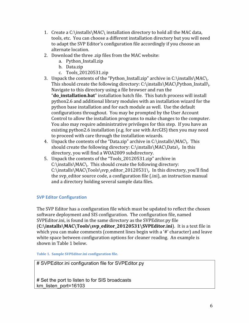
1. Create a C:\installs\MAC\ installation directory to hold all the MAC data, tools, etc. You can choose a different installation directory but you will need to adapt the SVP Editor’s configuration file accordingly if you choose an alternate location.
2. Download the three .zip files from the MAC website: a. Python_Install.zip b. Data.zip c. Tools_20120531.zip
3. Unpack the contents of the “Python_Install.zip” archive in C:\installs\MAC\. This should create the following directory: C:\installs\MAC\Python_Install\. Navigate to this directory using a file browser and run the “do_installation.bat” installation batch file. This batch process will install python2.6 and additional library modules with an installation wizard for the python base installation and for each module as well. Use the default configurations throughout. You may be prompted by the User Account Control to allow the installation programs to make changes to the computer. You also may require administrative privileges for this step. If you have an existing python2.6 installation (e.g. for use with ArcGIS) then you may need to proceed with care through the installation wizards.
4. Unpack the contents of the “Data.zip” archive in C:\installs\MAC\. This should create the following directory: C:\installs\MAC\Data\. In this directory, you will find a WOA2009 subdirectory.
5. Unpack the contents of the “Tools_20120531.zip” archive in C:\installs\MAC\. This should create the following directory: C:\installs\MAC\Tools\svp_editor_20120531\. In this directory, you’ll find the svp_editor source code, a configuration file (.ini), an instruction manual and a directory holding several sample data files.
SVP Editor Configuration The SVP Editor has a configuration file which must be updated to reflect the chosen software deployment and SIS configuration. The configuration file, named SVPEditor.ini, is found in the same directory as the SVPEditor.py file (C:\installs\MAC\Tools\svp_editor_20120531\SVPEditor.ini). It is a text file in which you can make comments (comment lines begin with a ‘#’ character) and leave white space between configuration options for cleaner reading. An example is shown in Table 1 below. Table 1. Sample SVPEditor.ini configuration file.
# SVPEditor.ini configuration file for SVPEditor.py # Set the port to listen to for SIS broadcasts km_listen_port=16103

7
# Set the listen interval for SIS broadcasts km_listen_timeout=1 # Set the port to listen to for Sippican input sippican_listen_port=2002 # Set the listen interval for Sippican input sippican_listen_timeout=1 # Set the IP address to send SVP casts to to multiple recipients # with variable protocols (SIS only for now). This is for version # 1.0.1. All rows are parsed, each row represents one recipient. # Information is in the following format: # "name":IP:port:protocol # Note that SIS will only receive SVP input on port 4001. sv_v2_recipient_ip="Kilo Moana EM122":10.23.11.108:4001:SIS sv_v2_recipient_ip="Kilo Moana EM710":10.23.11.106:4001:SIS # Set oceanographic data sources for various # functions in the software, e.g. Profile extension, # Salinity augmentation for XBT and data source for the # SVP Server extension_source=WOA09 salinity_source=WOA09 server_source=WOA09 # upcast/downcast data selection for CTDs and Velocimeters. # Currently supported options are ‘down’ or ‘up’. up_or_down_cast=down # Write out cast metadata automatically when sending a cast over network write_metadata_on_send=True # Path to World Ocean Atlas 2009 grid files woa_path=C:\installs\MAC\Data\WOA2009 You will need to modify the SVP Editor’s configuration file to use all of the available functionality. At this stage, you only need to modify the file if you have installed the WOA2009 data directory somewhere other than C:\installs\MAC\Data\WOA2009. If this is the case, then follow open the configuration file for editing in your text editor of choice and update the “woa_path” variable to point to the directory where the World Ocean Atlas data set was installed (step 4 in the installation sequence above). Once your configuration file has been updated, you can test the installation by navigating in a browser window to C:\installs\MAC\Tools\svp_editor_20120531\

8
and double-‐clicking on SVPEditor.py to launch the editor, you should see a window as shown in Fig. 1. At this point, it is helpful to create a desktop shortcut to the SVPEditor.py file.
Figure 1. SVP Editor main window view.
SIS Configuration To fully take advantage of all the SVP Editor functionality, SIS must be configured to send a subset of datagrams to the software. The required datagrams are listed below along with a brief description of how they are used by the SVP Editor: • Position (‘P’, 0x50): Provides date/position information for use with Server
mode. • Sound speed profile (‘U’, 0x55): Allows SVP Editor to ascertain whether or not
a sound speed profile transmission was successful or not. • XYZ88 (‘X’, 0x58): Provides the surface sound speed used in beam forming and
steering and also provides the transducer draft. Both of these values are used when augmenting sound speed profiles with the measured surface sound speed value.
9
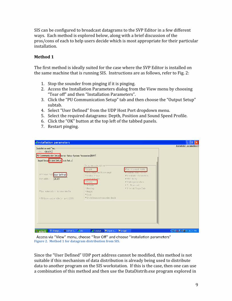
SIS can be configured to broadcast datagrams to the SVP Editor in a few different ways. Each method is explored below, along with a brief discussion of the pros/cons of each to help users decide which is most appropriate for their particular installation. Method 1 The first method is ideally suited for the case where the SVP Editor is installed on the same machine that is running SIS. Instructions are as follows, refer to Fig. 2:
1. Stop the sounder from pinging if it is pinging. 2. Access the Installation Parameters dialog from the View menu by choosing
“Tear off” and then “Installation Parameters”. 3. Click the “PU Communication Setup” tab and then choose the “Output Setup”
subtab. 4. Select “User Defined” from the UDP Host Port dropdown menu. 5. Select the required datagrams: Depth, Position and Sound Speed Profile. 6. Click the “OK” button at the top left of the tabbed panels. 7. Restart pinging.
Figure 2. Method 1 for datagram distribution from SIS.
Since the “User Defined” UDP port address cannot be modified, this method is not suitable if this mechanism of data distribution is already being used to distribute data to another program on the SIS workstation. If this is the case, then one can use a combination of this method and then use the DataDistrib.exe program explored in

10
Method 3 to split the data streams coming in to the output port between the various software packages that require these data. This may not be suitable if the other software package(s) cannot be reconfigured to accept data input from another port. The default output port appears to vary with the echosounder model, Table 1 summarizes the port addresses observed to date. Table 2. User-defined output port addresses for various Kongsberg Maritime multibeam echosounders.
Model User Defined datagram ouput port EM2040 Unknown EM710 16103 EM302 16343 EM122 16103 Method 2 The second method uses a more generalized data distribution feature of SIS that allows for transmission to other computers on the network by specifying the IP address of the recipient machine and the port that the machine would like the data delivered to. One can also tailor the transmission rate, for example to reduce high data rates associated with some sensors. Instructions are as follows, refer to Fig. 3:

11
Figure 3. Method 2 for datagram distribution from SIS.

12
1. From the “Tools” menu, choose “Custom…” and then “Datagram Distribution”.
2. Choose the datagram from the drop down menu, starting with Position (P). 3. Type in the IP address of the remote machine where SVP Server is installed,
immediately followed by a colon (:), immediately followed by the port number that the data should be delivered to on the remote machine. For example: 192.168.1.67:16103.
4. Click the Subscribe button. 5. Repeat Steps 2-‐4 for the SVP (U) datagram and the XYZ88 datagram. Be
careful NOT to choose the SVP (W) datagram by accident. There are three drawbacks to this method:
1. SIS needs to be restarted for the changes to take effect. Method 1 only requires you to stop pinging.
2. It has been found that it is not always possible to unsubscribe from datagram distribution using the interface.
3. The software program that allows for user input does not appear to validate the input. Mistakes made during input can impact on datagram distribution and cannot be easily undone because of (2).
Method 3

13
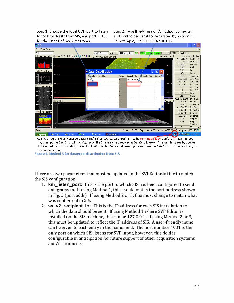
The third method relies on either methods 1 or 2 being implemented already and cannot work without either of these two being in place already. This third approach simply allows for more options on redistributing data when faced with the situation where multiple software packages are competing for data broadcasts from SIS. Method 1 can only support data output on port 16103 so it can be followed directly using the instructions above before starting this portion. If Method 2 is chosen as the starting point, then the IP address chosen in Method 2 must be localhost. The output port must be different than 16103. This last method requires the use of a standalone program, named DataDistrib.exe, which is bundled with SIS during the installation of SIS. The program resides in C:\Program Files\Kongsberg Maritime\SIS\bin\. In the same directory, you’ll find a DataDistrib.ini file that retains all the subscription and delivery information. The file can be edited with care or the user can input parameters through the graphical interface through the following instructions (refer to Fig. 4).
1. If the program is running already, click the icon in the task bar to launch the graphical interface. If it is not running, navigate to C:\Program Files\Kongsberg Maritime\SIS\bin\ and double click on DataDistrib.exe to launch the program.
2. Find the first empty row and enter the UDP port to which SIS is distributing data in the left most column. Hit the “Enter” button to finalize the entry.
3. Staying in the same row, click on the fourth column and type in the IP address of the remote machine where SVP Server is installed, immediately followed by a colon (:), immediately followed by the port number that the data should be delivered to on the remote machine. For example: 192.168.1.67:16103. Again, hit the “Enter” key to finalize the entry.
4. If SIS is pinging and distributing the data, you should see the packet count increase steadily in the third column.
This method has a few drawbacks:
1. You must remember to start the DataDistrib.exe program every time you restart the SIS workstation. It is possible to have it start automatically at startup by dragging the program icon into the Start menu. However, see (2).
2. The program can be accidentally closed quite easily; this will stop all data distribution.
3. It has been found that the initialization file can sometimes become corrupt after updating the entries in the distribution table OR if the program is accidentally run twice. Once entries are finalized, the initialization file used by the program can be made “read only” to prevent corruption. This may lead to confusion for others using the same program at a later date, as it will not support additional entries.
14
Figure 4. Method 3 for datagram distribution from SIS.
There are two parameters that must be updated in the SVPEditor.ini file to match the SIS configuration:
1. km_listen_port: this is the port to which SIS has been configured to send datagrams to. If using Method 1, this should match the port address shown in Fig. 2 (port addr). If using Method 2 or 3, this must change to match what was configured in SIS.
2. sv_v2_recipient_ip: This is the IP address for each SIS installation to which the data should be sent. If using Method 1 where SVP Editor is installed on the SIS machine, this can be 127.0.0.1. If using Method 2 or 3, this must be updated to reflect the IP address of SIS. A user-‐friendly name can be given to each entry in the name field. The port number 4001 is the only port on which SIS listens for SVP input, however, this field is configurable in anticipation for future support of other acquisition systems and/or protocols.

15
Operating Instructions
Introduction There are two mutually exclusive modes of operation of this software:
1. SVP/CTD/XBT/XSV processing mode: convert data from imported data files, graphically edit, augment with World Ocean Atlas (WOA) salinity and extrapolate cast with WOA. Once complete, the cast is transmitted to the echosounder for immediate application (i.e. the SIS SVP Editor program is not required).
2. Server mode: deliver WOA derived synthetic sound speed profiles to the sounder in a continuous manner while in transit using the reported position as input to the WOA lookup.
Both modes begin by running the SVP Editor by double-‐clicking on the Desktop shortcut icon. The main SVP Editor window will appear (see Fig. 5). If SIS has been configured to output the datagrams as specified in the Installation section, the right side of the status bar will update with the position and surface sound speed. Note that the surface sound speed will only update if the echosounder is pinging since the surface sound speed information can only be extracted from the depth datagram.

16
Figure 5. SVP Editor main window view.
At this point, the user can either process SVP/CTD/XBT/XSV data or they can launch the SVP Server. Both of these options are explored below.
Processing SVP/CTD/XBT/XSV
Importing data From the File menu, select Import…, a file selection dialog will allow you to choose a .EDF (or .edf) file. There are sample data files in C:\installs\MAC Tools\svp_editor\sample_data\ directory. The file type filter can be used to choose the file type. Select the desired file and click okay. This will update the plot panels with the sound speed, temperature and salinity profiles drawn in solid blue (left to right, respectively, see Fig. 6). During the import stage, the geographic position and date in the input file are used to query the WOA to provide mean sound speed, temperature and salinity profiles that provide some context during data editing. These are drawn in drawn in dashed magenta. It is important that the cast positional metadata is correct for this lookup to be correct.
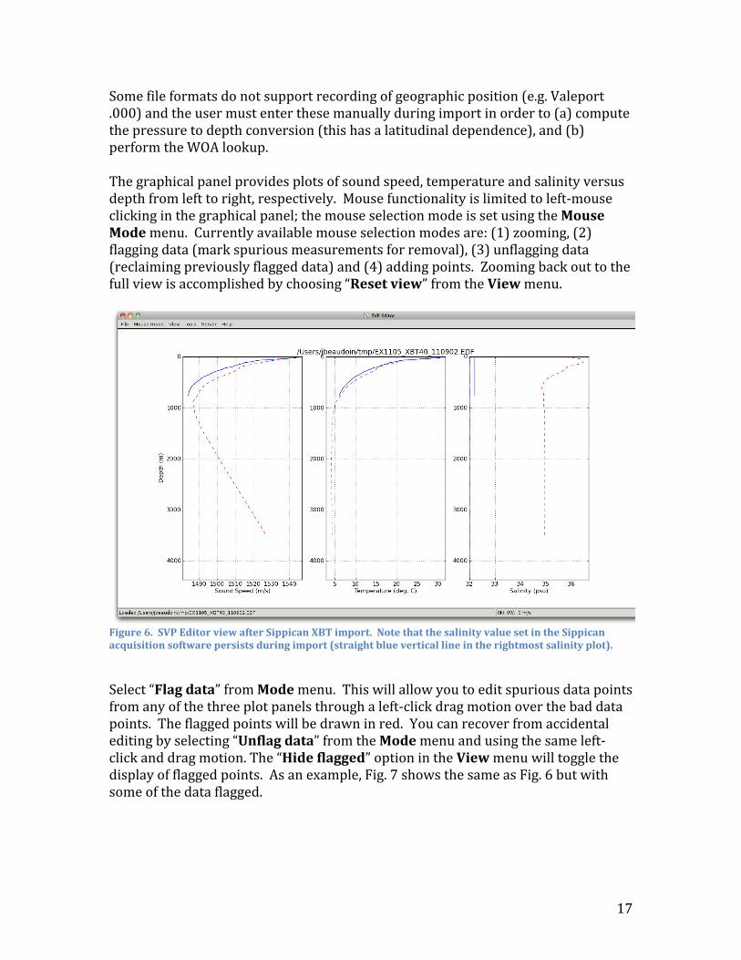
17
Some file formats do not support recording of geographic position (e.g. Valeport .000) and the user must enter these manually during import in order to (a) compute the pressure to depth conversion (this has a latitudinal dependence), and (b) perform the WOA lookup. The graphical panel provides plots of sound speed, temperature and salinity versus depth from left to right, respectively. Mouse functionality is limited to left-‐mouse clicking in the graphical panel; the mouse selection mode is set using the Mouse Mode menu. Currently available mouse selection modes are: (1) zooming, (2) flagging data (mark spurious measurements for removal), (3) unflagging data (reclaiming previously flagged data) and (4) adding points. Zooming back out to the full view is accomplished by choosing “Reset view” from the View menu.
Figure 6. SVP Editor view after Sippican XBT import. Note that the salinity value set in the Sippican acquisition software persists during import (straight blue vertical line in the rightmost salinity plot).
Select “Flag data” from Mode menu. This will allow you to edit spurious data points from any of the three plot panels through a left-‐click drag motion over the bad data points. The flagged points will be drawn in red. You can recover from accidental editing by selecting “Unflag data” from the Mode menu and using the same left-‐click and drag motion. The “Hide flagged” option in the View menu will toggle the display of flagged points. As an example, Fig. 7 shows the same as Fig. 6 but with some of the data flagged.

18
Figure 7. View of data after user has flagged bad data points (drawn in red).
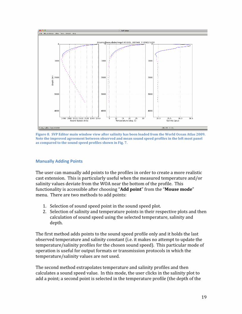
Augmenting with WOA Salinity/Temperature Select “XBT load salinity…” from the Tools menu. The dashed magenta WOA salinity profile is used to augment the XBT temperature measurement as shown in Fig. 8. The vertical resolution of the WOA09 grids is coarse compared to the sampling interval of the measured data, so the salinity estimates are linearly interpolated to the depths associated with each of the temperature observations in the measured profile. The right-‐most salinity plot will update with a salinity profile and the left-‐most sound speed plot will now be updated with sound speed recalculated using the new salinity estimates. Sound speed is calculated using the UNESCO equation (Fofonoff and Millard, 1983). In the case of an XSV file, the user can augment the measured sound speed with WOA temperature and salinity through the “XSV load temperature/salinity…” option under the Tools menu. The sound speed is NOT recalculated, the temperature and salinity are meant merely for SIS to compute more reasonable transmission loss corrections for improved backscatter normalization. The software will disallow application of WOA salinity to XSV profiles and will also disallow application of WOA temperature/salinity to XBT profiles.
19
Figure 8. SVP Editor main window view after salinity has been loaded from the World Ocean Atlas 2009. Note the improved agreement between observed and mean sound speed profiles in the left most panel as compared to the sound speed profiles shown in Fig. 7.
Manually Adding Points The user can manually add points to the profiles in order to create a more realistic cast extension. This is particularly useful when the measured temperature and/or salinity values deviate from the WOA near the bottom of the profile. This functionality is accessible after choosing “Add point” from the “Mouse mode” menu. There are two methods to add points:
1. Selection of sound speed point in the sound speed plot. 2. Selection of salinity and temperature points in their respective plots and then
calculation of sound speed using the selected temperature, salinity and depth.
The first method adds points to the sound speed profile only and it holds the last observed temperature and salinity constant (i.e. it makes no attempt to update the temperature/salinity profiles for the chosen sound speed). This particular mode of operation is useful for output formats or transmission protocols in which the temperature/salinity values are not used. The second method extrapolates temperature and salinity profiles and then calculates a sound speed value. In this mode, the user clicks in the salinity plot to add a point; a second point is selected in the temperature profile (the depth of the

20
first point in the salinity plot will be adjusted to match the depth of the second click). A third click in the sound speed plot will then chosen depth/temperature/salinity values from the temperature/salinity plots to compute the new sound speed point (the depth from the last click in the sound speed plot is NOT used). The user-‐selected temperature/salinity points are drawn in green until the sequence is completed, as shown in Fig. 9. Multipoint extensions are achieved through repeating the above sequence. If a deep extension that exceeds the view limits is required, repeatedly clicking near the bottom of the plots will automatically adjust the view bounds, allowing the user to reach the required depth with only a few mouse clicks typically.
Figure 9. Manual extension of temperature and salinity profiles to circumvent mismatch between the measured and WOA temperature at depth.
Applying Surface Sound Speed Now select “Load Surface SSP…” from the Tools menu. If configured to receive data from SIS, the surface sound speed and transducer draft from the depth datagram broadcast will be used to create a surface layer of thickness equal to the transducer draft and of sound speed equal to the value used in beam forming, this presumably being from the surface sound speed probe. See Fig. 10 for an example. If neither the surface sound speed or transducer draft values are available from a SIS data broadcast, the software will prompt the user to input values for both. The intent of this feature is to keep the sound speed profile and sound speed sensor values similar such that the numerical display monitors in SIS do not warn against

21
sound speed discrepancies between the two measurements. For those wary of this practice, it should be noted that this is done internally in SIS during their ray tracing operations regardless of this external processing stage: “transducer depth sound speed is used as the initial entry in the sound speed profile used in the ray tracing calculations” (Kongsberg, 2012). Having it done externally in this manner keeps the system from warning against discrepancies based on (a) the uncertainty in XBT temperature measurements (+/-‐0.1°C, roughly equivalent to +/-‐0.4 m/s) and/or (b) inadequate choice of salinity in the Sippican acquisition system or (c) deviations of true salinity from the mean surface salinity in the WOA.
Figure 10. Zoomed in view showing surface layer created through application of measured surface sound speed to a surface layer as thick as the transducers are deep. In this particular example, a surface layer of 20 m was created through manual entry of data when prompted by the software. The temperature and salinity profiles are unaffected by this operation and it is only the sound speed that is updated.
Extending with WOA Salinity/Temperature Now select “Extend cast…” from the Tools menu and the observed cast will extended as much as possible using the WOA profile and the three plot panels will be updated as shown in Figure 11. Details of the extrapolation algorithm can be found in Appendix A. If desired or necessary, edit any discontinuities between the cast and the extension in the vicinity of the maximum observation depth. The extension will only go as deep as 5,500 m as this is the deepest depth layer that the WOA supports. When files are transmitted to SIS (or are exported in .asvp format)

22
the software extends the profile to 12,000 m depth to meet SIS SVP input criteria and there is no need for the user do this.
Figure 11. SVP Editor main window view after extending cast using World Ocean Atlas 2009 (compare maximum depth with that of Fig. 8).
Transmitting Data to SIS Select “Send Profile…” from the Tools menu to send the cast to SIS. This procedure will format the temperature and salinity profiles into the Kongsberg Maritime format described in Kongberg (2012). The WOA09 grids only extend to 5,500 m thus the profile undergoes a final extrapolation to a depth of 12,000 m to satisfy SIS input criteria, this is done with temperature and salinity values measured in the Mariana Trench by Taira et al. (2005), see Appendix A for more discussion on this. Since SIS input profiles have a limit on the maximum allowable number of data points, the sound speed profile is thinned using a modified version of the Douglas-‐Peucker line reduction method as described in Beaudoin et al. (2011). The algorithm begins with a small tolerance and increases it linearly until the number of points in the profile falls below the maximum allowed by SIS. The cast header is formatted to instruct SIS to accept the profile for immediate application without launching the Kongsberg SVP Editor (Kongsberg, 2012). Once the cast has been prepared for transmission, it is sent to SIS via UDP transmission over the network. If SIS receives the profile and accepts it, it will rebroadcast the SVP datagram. The SVP Editor waits for this rebroadcast to ensure

23
reception of the cast. The profile that was rebroadcasted from SIS is compared against that which was sent. If they match, then the transmission is considered successful. If there is a discrepancy, or if no rebroadcast profile is received, the user is notified that reception could not be confirmed. The lower left status bar will notify the user of the various stages of this verification process. In deep water, the rebroadcast event may take several seconds to occur and the software will wait up to 30 seconds for reception of the rebroadcasted SVP. All other functionality is suspended during this wait period. For installations with multiple clients, the software will deliver the cast sequentially to all clients. Failure on transmission to one client will not interfere with other clients.
Speeding Things Up Once configured to receive data from SIS, many of the items under the Tools menu require no interaction or input at all. For this reason, the “Express…” option has been added for users who are comfortable with the post-‐processing steps that have been shown thus far. The “Express…” option bundles all of the above processing stages into a single user initiated action and finishes by delivering the profile to SIS. It chooses the appropriate augmentation for XBT and XSV. Other sensor formats ignore the XBT/XSV temperature/salinity augmentation steps. WARNING: There will be no opportunity for the user to edit any discontinuities based on the WOA extension so the data should be examined briefly to see how well the extrapolation will do prior to launching this sequence of processing. The user should also remove any outlier measurements prior to selecting “Express…”. Referring back to Fig. 6, this particular cast would be a good candidate for the “Express…” mode based on the fact that (a) it does not suffer from temperature spikes, and (b) there is generally good agreement between the observed temperatures and the WOA profile.
Running the SVP Server The Server mode of operation is meant for transits during which perhaps one XBT per day might be fired. For much of the world oceans, using the WOA is a reasonable substitute for in situ measurements (Beaudoin, 2011). Given that transit data are usually a lower priority, the SVP Server supports continuous underway logging of multibeam data that are refraction corrected using the mean temperature and salinity profiles provided by WOA. Future additions to the software will include some guidance as to whether or not the particular area of ocean that you are working in is suitable for use with the server mode.
24
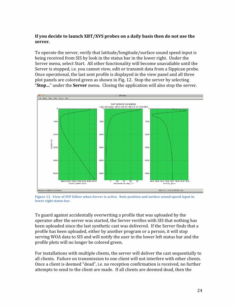
If you decide to launch XBT/XVS probes on a daily basis then do not use the server. To operate the server, verify that latitude/longitude/surface sound speed input is being received from SIS by look in the status bar in the lower right. Under the Server menu, select Start. All other functionality will become unavailable until the Server is stopped, i.e. you cannot view, edit or transmit data from a Sippican probe. Once operational, the last sent profile is displayed in the view panel and all three plot panels are colored green as shown in Fig. 12. Stop the server by selecting “Stop…” under the Server menu. Closing the application will also stop the server.
Figure 12. View of SVP Editor when Server is active. Note position and surface sound speed input in lower right status bar.
To guard against accidentally overwriting a profile that was uploaded by the operator after the server was started, the Server verifies with SIS that nothing has been uploaded since the last synthetic cast was delivered. If the Server finds that a profile has been uploaded, either by another program or a person, it will stop serving WOA data to SIS and will notify the user in the lower left status bar and the profile plots will no longer be colored green. For installations with multiple clients, the server will deliver the cast sequentially to all clients. Failure on transmission to one client will not interfere with other clients. Once a client is deemed “dead”, i.e. no reception confirmation is received, no further attempts to send to the client are made. If all clients are deemed dead, then the
25
server stops and notifies the user. Note that SIS will accept and rebroadcast SVP datagrams even if it is not pinging.
Additional Functionality
Creating New WOA profile If you’d like to upload a single WOA profile to SIS, you can select “New WOA…” under the “File” menu. A series of question dialogs will allow you to either use the SIS position input for the query position OR you can provide your own position input. You can then apply a surface sound speed and send the cast via the “Send Profile…” option under the “Tools” menu. The new cast will be given the filename WOA_synthetic_cast.svp.
Exporting Files Any file that is loaded into the SVP Editor can be exported by accessing the “Export…” option under the file menu. Several formats are currently supported, please contact the MAC to request support of additional export formats.
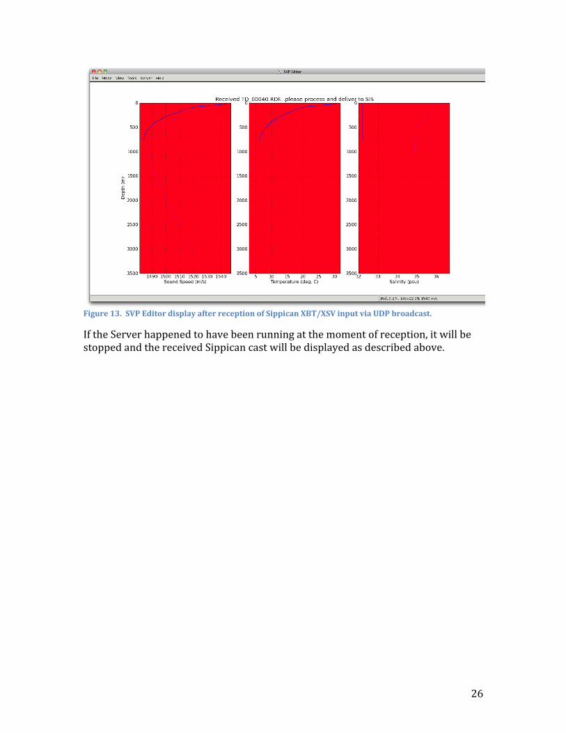
Receiving Sippican XBT/XSV Files via UDP The SVP Editor is configured to always listen on port 2002 for UDP input of Sippican XBT/XSV casts. This port number can be changed in the SVPEditor.ini file. There does not currently exist any mechanism to broadcast data via UDP via the Sippican acquisition software, however, this capability has been included to accommodate vessels who use UDP network broadcasts to log data from various systems. Note that a single Sippican cast can sometimes exceed the maximum buffer size for UDP packet transmissions. If software is written to transmit Sippican data files via UDP, this limitation should be kept in mind. SVP Editor currently only accepts transfer of a single UDP packet thus transmission software may need to reduce the data by thinning the profile. Upon reception of a Sippican data file, the SVP Editor will color code the panels red to indicate that operator intervention is required in order to further process the data and deliver it to SIS, as shown in Fig. 13. Once the cast has been processed and delivered, the panel color coding will return to the normal white background.
26
Figure 13. SVP Editor display after reception of Sippican XBT/XSV input via UDP broadcast.
If the Server happened to have been running at the moment of reception, it will be stopped and the received Sippican cast will be displayed as described above.

27
Additional Notes & Caveats The World Ocean Atlas 2009 data set has been installed in C:\installs\MAC Tools\MAC data\ and an environment variable is added during installation to help SVP Editor find this data set automatically without user direction. If the data are relocated, then the environment variable must be updated or removed. Eventually this will be a user-‐configurable parameter that can be saved in the configuration file. Seeing as this is relatively new software, the user should become comfortable with what signs to look for in SIS in order to confirm that profiles are indeed being received, be it from a processed SVP/CTD/XBT cast or from the Server. The following indications are useful for monitoring reception of sound speed profiles in SIS:
1. The SVP profile filename will be updated in the run time parameters menu. The profile filename will be of the form YYYYMMDD_HHMMSS.asvp. The date and time fields are populated based on the time stamp in the profile that was received from the SVP Editor. In the case of measured casts, this is the time of acquisition, as found in the input file. In the case of synthetic WOA profiles, the date/time is based on the time of transmission of the cast (using the computer clock where SVP Editor is installed).
2. SIS will create several files in the last location that it loaded a sound speed profile from.
3. The SVP display window, if being viewed in SIS, will update with the new cast.
In the event that a cast is rejected, SIS will launch a warning dialog to indicate that the cast it received was rejected. In this case, please note the warning message and send it, along with the offending data file, to [email protected].

28
References Antonov, J. I., D. Seidov, T. P. Boyer, R. A. Locarnini, A. V. Mishonov, H. E. Garcia, O. K.
Baranova, M. M. Zweng, and D. R. Johnson, 2010. World Ocean Atlas 2009, Volume 2: Salinity. S. Levitus, Ed. NOAA Atlas NESDIS 69, U.S. Government Printing Office, Washington, D.C., 184 pp.
Beaudoin, J., Smyth, S., Furlong, A., Floc’h, H. and Lurton, X., 2011. Streamlining
Sound Speed Profile Pre-‐Processing: Case Studies and Field Trials, US Hydro Conference 2011, April 25-‐29, Tampa, FL, USA.
Fofonoff, N. P., and Millard, R. C. (1983). "Algorithms for computation of
fundamental properties of seawater." Rep. No. 44, Division of Marine Sciences, UNESCO, Place de Fontenoy, 75700, Paris.
Kongsberg (2012). " EM Series Multibeam echo sounders Datagram Formats,
Revision O" Kongsberg Maritime AS, Horten, Norway. Locarnini, R. A., A. V. Mishonov, J. I. Antonov, T. P. Boyer, H. E. Garcia, O. K. Baranova,
M. M. Zweng, and D. R. Johnson, 2010. World Ocean Atlas 2009, Volume 1: Temperature. S. Levitus, Ed. NOAA Atlas NESDIS 68, U.S. Government Printing Office, Washington, D.C., 184 pp.
Taira, K., Yanagimoto, D. and Kitagawa, S. (2005). “Deep CTD Casts in the Challenger
Deep, Mariana Trench”, Journal of Oceanography, Vol. 61, pp. 447-‐454.
29
Appendix A The World Ocean Atlas is a 3-‐dimensional grid of mean temperature and salinity for the worlds oceans that is based upon a large set of archived oceanographic measurements in the World Ocean Database. More information about the World Ocean Atlas 2009 can be found online at: http://www.nodc.noaa.gov/OC5/WOA09/pr_woa09.html Vertical Extrapolation The cast extrapolation algorithm will vertically extend temperature and salinity profiles as deep as possible using the estimates immediately local to the area of the cast in the World Ocean Atlas. The extension algorithm uses a nearest neighbor lookup in each of the 33 depth levels in the grids within a 3x3 grid node search box centered on the cast’s geographic position. This is roughly equivalent to a search radius of 1.5° or 90 NM at the equator, note that this grid node search box becomes rapidly narrower in the east-‐west direction with latitude. The nearest-‐neighbor geodetic distance is, however, correctly computed and the nearest neighbor will indeed be the geographically most proximal grid node; the only shortcoming is that the lookup will ignore potentially closer data in the east-‐west direction at high latitudes. Future updates to the WOA09 extraction algorithms will remedy this shortcoming. The search radius is set this large to enable the extension to at least estimate deeper temperature and salinity values in the case where the true depth at the requested location is significantly larger than the coarse depth reported in the WOA09 grid for that location (the WOA09 grid depth will generally always be smaller than the true depth). The search algorithm will not respect topographic boundaries and may extrapolate profiles using data from a neighboring oceanographic basin. Future versions of the algorithm will address this shortcoming as well, likely with the use of the basin mask file provided with the WOA09 data set. The final extrapolation to a depth of 12,000 m is done using the values measured by Tairo et al. (2005) in Challenger Deep. This could be improved by searching for the nearest neighbor grid node at the deepest level observed in the basin using the basin mask file. Data Access The netCDF temperature and salinity grids used by SVP Editor can be accessed from http://www.nodc.noaa.gov/OC5/WOA09/netcdf_data.html The files required are: temperature_annual_1deg.nc temperature_seasonal_1deg.nc

30
temperature_monthly_1deg.nc salinity_annual_1deg.nc salinity_seasonal_1deg.nc salinity_monthly_1deg.nc Basin and land/sea masks can be downloaded from http://www.nodc.noaa.gov/OC5/WOA09/masks09.html The files required are basin.msk, landsea.msk and mixnumber.msk. Currently, the SVP Editor requires only the landsea.msk file, however, future versions may use the other masks so it is advised to download these as well.