sustainable pavement asset management based …
TRANSCRIPT

SUSTAINABLE PAVEMENT ASSET MANAGEMENT BASED ON LIFE CYCLE MODELS AND OPTIMIZATION METHODS
by
Han Zhang
A dissertation submitted in partial fulfillment of the requirements for the degree of
Doctor of Philosophy (Natural Resources and Environment)
in The University of Michigan 2009
Doctoral Committee: Associate Professor Gregory A. Keoleian, Chair Professor Jonathan W. Bulkley Professor Victor C. Li Professor Michael R. Moore

© Han ZhangAll Rights Reserved
2009

ii
DEDICATION
To my parents, who gave me a love of life
To my fiancée,
who gave me a life of love

iii
ACKNOWLEDGEMENTS
I would like to thank my advisor, Professor Gregory A. Keoleian. Without his
support, patience, and encouragement throughout the past years I could have never
completed this work. I have been fortunate to have an advisor who gave me the freedom
to explore on my own and at the same time guided me in the right direction. I am deeply
indebted to him and grateful for his guidance.
I would like to thank my dissertation committee members, Professor Jonathan W.
Bulkley, ProfessorVictor C. Li, and Professor Michael R. Moore for their valuable
guidance and support based on their expertise in areas of material science,
microeconomics, and optimization.
I wish to acknowledge the National Science Foundation for funding of Materials
Use: Science, Engineering, and Society (NSF MUSES) Biocomplexity Program Grant
(CMS-0223971) and the Michigan Department of Transportation, particularly Mr.
Benjamin Krom, for providing the necessary data and support for my research.
I would also like to thank Dr. Michael D. Lepech. Through the three years we
worked together closely, he provided me tremendous help and shared his expertise of
ECC. I couldn’t have finished my research without his knowledge, help and support.
I would like to thank Dr. Alissa Kendall who helped me to develop the life cycle
model and shared her experience of finishing a doctoral study.

iv
I would like to thank my colleagues in the Center for Sustainable Systems and
many other friends for their unconditional support and friendship.
I will also be thankful to my former advisor at Tsinghua University in China,
Professor Zheng Li, the Climate Crusader named by Time magazine. He is the one who
first showed me the wonders and frustrations of scientific research. Without his sincere
advice and encouragement, I would not have the chance and courage to pursue the
doctoral degree. His dedication to research will inspire me forever.
Most importantly, I could never have attempted any of this without the love and
support of the greatest parents, Shuye and Huafang. I am deeply appreciative of their
faith in me no matter what I have chosen to do. They are always supporting and
providing the best they can do to enlarge my vision and enrich my life.
Last, but far from least, I would like to thank my fiancée Dr. Yuanyuan Zhou for
her love, understanding, and consistent support for the past ten years. She is always there
cheering me up and standing behind me during both times of excitement and frustration.
v
TABLE OF CONTENTS
DEDICATION....................................................................................................................II
ACKNOWLEDGEMENTS.............................................................................................. III
LIST OF FIGURES .........................................................................................................VII
LIST OF TABLES............................................................................................................. X
LIST OF APPENDICES................................................................................................... XI
ABSTRACT ....................................................................................................................XII
CHAPTER 1 INTRODUCTION ........................................................................................ 1
1.1 Motivation......................................................................................................... 1
1.2 Research Objectives.......................................................................................... 7
1.3 Organization...................................................................................................... 8
References................................................................................................................ 11
CHAPTER 2 INTEGRATED LIFE CYCLE ASSESSMENT AND LIFE CYCLE COST ANALYSIS MODEL .................................................................................. 13
2.1 Introduction..................................................................................................... 14
2.2 Methodology................................................................................................... 18
2.2.1 System Definition ............................................................................... 18
2.2.2 Integrate LCA-LCCA Model.............................................................. 21
2.3 Results and Discussions.................................................................................. 36
2.3.1 Life Cycle Assessment Results............................................................ 36
2.3.2 Life Cycle Cost Analysis Results ....................................................... 41

vi
2.3.3 Sensitivity Analysis ............................................................................ 43
2.4 Conclusions..................................................................................................... 45
References................................................................................................................ 47
CHAPTER 3 PROJECT-LEVEL PAVEMENT ASSET MANAGEMENT SYSTEM USING LIFE CYCLE OPTIMIZATION.................................................... 52
3.1 Introduction..................................................................................................... 53
3.2 Methodology................................................................................................... 55
3.2.1 System Definition ............................................................................... 55
3.2.2 Pavement Overlay Deterioration Model ............................................. 56
3.2.3 Life Cycle Optimization ..................................................................... 57
3.2.4 Life Cycle Optimization Model Operation ......................................... 60
3.3 Results and Discussions.................................................................................. 62
3.3.1 Life Cycle Optimization Results......................................................... 62
3.3.2 Traffic Growth Scenario ..................................................................... 66
3.4 Conclusion ...................................................................................................... 68
References................................................................................................................ 70
CHAPTER 4 MULTI-OBJECTIVE AND MULTI-CONSTRAINT OPTIMIZATION IN PROJECT-LEVEL PAVEMENT ASSET MANAGEMENT: INFORMING POLICY AND ENHANCING SUSTAINABILITY................................... 72
4.1 Introduction..................................................................................................... 73
4.2 Methodology................................................................................................... 76
4.2.1 Expanded Project-Level Pavement Asset Management System ........ 76
4.2.2 Multi-Constraint Optimization Model ................................................ 77
4.2.3 Multi-Objective Optimization Model ................................................. 80
4.3 Pavement Asset Management System Results – Pavement Overlay Case Study 82
4.3.1 Multi-Constraint Optimization Result ................................................ 82
vii
4.3.2 Multi-Objective Optimization Result ................................................. 84
4.4 Discussion....................................................................................................... 85
4.5 Conclusion ...................................................................................................... 89
References................................................................................................................ 91
CHAPTER 5 NETWORK-LEVEL PAVEMENT ASSET MANAGEMENT SYSTEM INTEGRATED WITH LIFE CYCLE ANALYSIS AND LIFE CYCLE OPTIMIZATION......................................................................................... 94
5.1 Introduction..................................................................................................... 95
5.2 Methodology................................................................................................... 98
5.2.1 Network-Level Pavement Asset Management System....................... 98
5.2.2 Priority Selection Model ................................................................... 100
5.2.3 GIS Model......................................................................................... 102
5.3 Case Study: Washtenaw County Pavement Network ................................... 104
5.3.1 Pavement Network Initialization ...................................................... 104
5.3.2 Network-level pavement asset management results ......................... 107
5.4 Conclusion .................................................................................................... 112
References.............................................................................................................. 115
CHAPTER 6 CONCLUSIONS AND FUTURE WORK............................................... 117
6.1 Conclusions................................................................................................... 117
6.1.1 Development of the Integrated Life Cycle Assessment and Life Cycle Cost Analysis Model......................................................................... 118
6.1.2 Project-Level Pavement Asset Management System ....................... 119
6.1.3 Multi-Objective and Multi-Constraint Optimization in Project-Level Pavement Asset Management ........................................................... 121
6.1.4 Network-Level Pavement Asset Management.................................. 122
6.2 Future Work .................................................................................................. 123
APPENDICES ................................................................................................................ 117
viii
LIST OF FIGURES
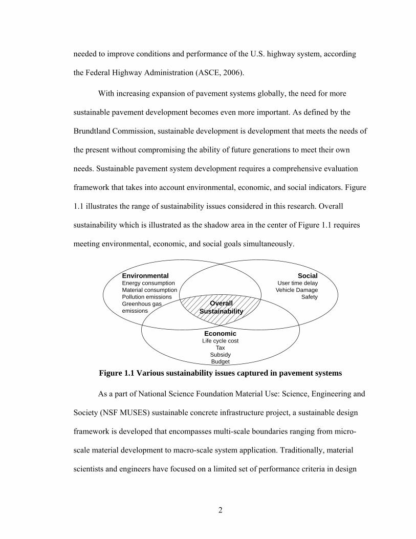
Figure 1.1 Various sustainability issues captured in pavement systems ............................ 2
Figure 2.1 Overlay structure and thickness in one direction ........................................... 19
Figure 2.2 Timeline and maintenance schedule for construction activities..................... 20
Figure 2.3 Integrated LCA-LCCA model framework ..................................................... 22
Figure 2.4 Material composition of concrete, HMA, and ECC materials ....................... 23
Figure 2.5 Primary energy consumption per volume of each material............................ 24
Figure 2.6 Distress index of each pavement .................................................................... 29
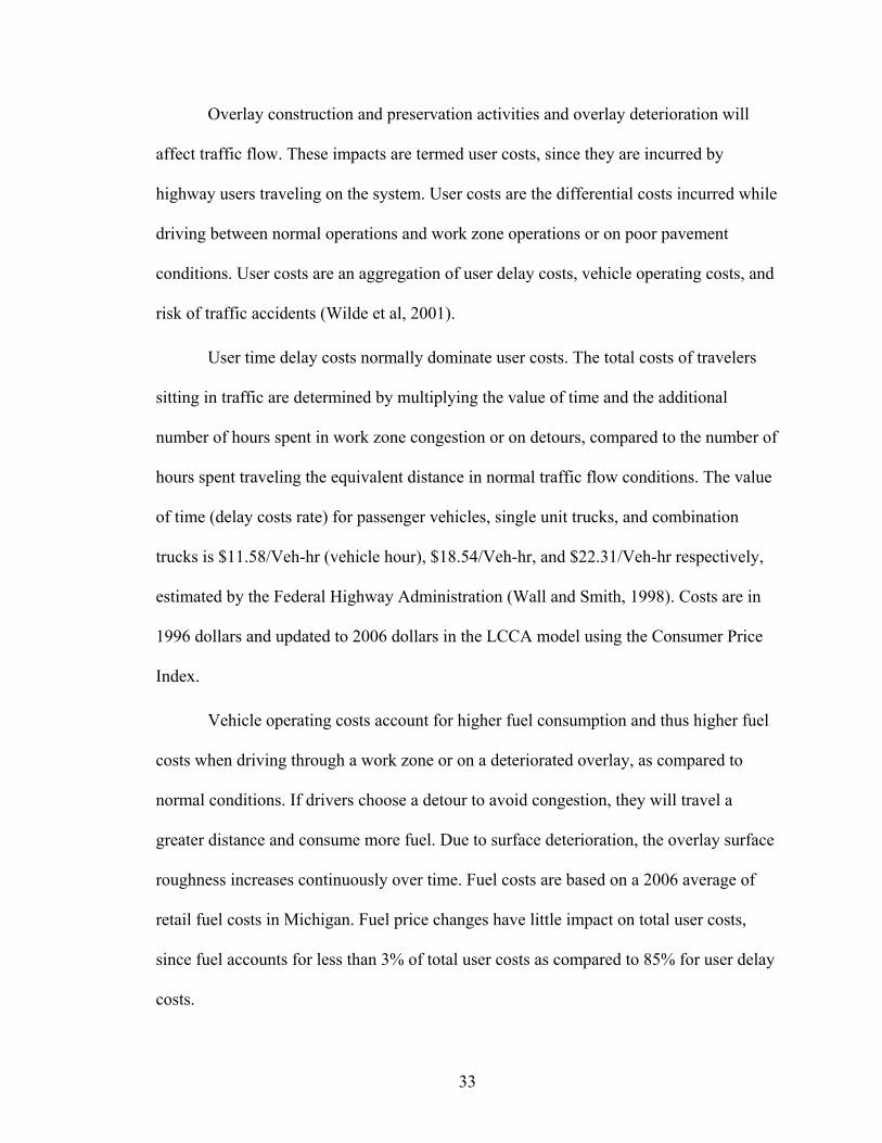
Figure 2.7 Life cycle energy consumption by life cycle phase........................................ 37
Figure 2.8 Greenhouse gas emissions by life cycle phase ............................................... 37
Figure 2.9 Air emissions by life cycle phase ................................................................... 39
Figure 2.10 Water pollutant emissions by life cycle phase ............................................. 40
Figure 2.11 Cumulative life cycle costs for overlay systems ........................................... 43
Figure 2.12 Energy consumption and life cycle costs at different traffic growth rate..... 44
Figure 2.13 Energy consumption and life cycle costs at different fuel economy improvements rate........................................................................................... 45
Figure 3.1 LCO model operation flowchart using dynamic programming ..................... 61
Figure 3.2 Optimal preservation strategies for three overlay systems............................. 63
Figure 3.3 Comparison of energy consumption, GHG emissions and costs for MDOT preservation strategies and optimal strategies for a. HMA, b. ECC, and c. Concrete overlay systems ............................................................................... 66
Figure 3.4 Optimal preservation strategies for three overlay systems with 2% annual traffic growth rate ........................................................................................... 67
ix
Figure 3.5 Life cycle results with different annual traffic growth rate............................ 68
Figure 4.1 Pavement asset management system framework ........................................... 75
Figure 4.2 The process of project-level pavement asset management system ................ 77
Figure 4.3 A hypothetical relationship between pavement condition and cost ............... 78
Figure 4.4 Multi-objective optimization and Pareto efficiency ....................................... 81
Figure 4.5 Optimal maintenance strategies based on different budget constraints.......... 83
Figure 4.6 Total life cycle cost based on different budget constraints for a 20 year analysis period ................................................................................................ 84
Figure 4.7 Pareto frontier for total energy consumption and total life cycle cost objectives for a 20 year analysis period.......................................................... 85
Figure 4.8 Optimal maintenance strategies based on different fuel prices ...................... 89
Figure 5.1 The integrated framework of the network-level PAMS................................. 98
Figure 5.2 Route event segmenting process .................................................................. 103
Figure 5.3 Union of two route event tables using dynamic segmentation..................... 104
Figure 5.4 GIS map and pavement network condition .................................................. 107
Figure 5.5 Average DI curves based on different preservation strategies ..................... 109
Figure 5.6 Total life cycle cost of different preservation strategies .............................. 110
Figure 5.7 Total life cycle cost based on different annual budget ................................. 111
Figure 5.8 Visualization of different attributes in GIS map .......................................... 112

x
LIST OF TABLES
Table 2.1 Total material consumption in each overlay system and associated data sources........................................................................................................................................... 21
Table 2.2 Total equipment usage during construction activities in hours ....................... 25
Table 2.3 Agency costs breakdown for overlay construction activities .......................... 32
Table 2.4 Air pollution damage costs by impacted region .............................................. 35
Table 2.5 Summary of life cycle impact results .............................................................. 41
Table 2.6 Life cycle costs for overlay systems ................................................................ 42
Table 3.1 Life cycle burdens of optimal preservation strategies for each overlay system........................................................................................................................................... 64
Table 5.1 Pavement segments information list .............................................................. 106
Table 5.2 Alternative preservation methods and unit costs ........................................... 108

xi
LIST OF APPENDICES
APPENDIX A LOW TRAFFIC VOLUME SCENARIOS........................................... 126
APPENDIX B DIFFERENT PAVEMENT CONDITION CONSTRAINTS............... 128
APPENDIX C DIFFERENT ANALYSIS PERIODS ................................................... 129
xii
ABSTRACT
SUSTAINABLE PAVEMENT ASSET MANAGEMENT BASED ON LIFE CYCLE MODELS AND OPTIMIZATION METHODS
Pavement systems provide critical infrastructure services to society but also pose
significant impacts related to high material consumption, energy inputs, and capital
investment. A new pavement asset management approach, using economic, social, and
environmental metrics, is proposed to enhance the sustainability of transportation
infrastructure systems.
This dissertation develops methods for evaluating and enhancing the
sustainability of pavement infrastructure. Four methods are presented: (1) integrated life
cycle assessment and life cycle cost analysis modeling of pavement overlay systems
comparing new material Engineered Cementitious Composites (ECC) to conventional
materials, (2) project-level pavement asset management system using life cycle
optimization, (3) multi-objective and multi-constraint optimization informing policy and
enhancing sustainability, and (4) network-level pavement asset management system
integrated with geographic information systems.
The integrated life cycle model results indicated that the application of ECC can
significantly improve overlay system sustainability. Compared to conventional concrete
and hot mixed asphalt (HMA) overlay systems, the ECC overlay system reduces life
cycle energy consumption by 15% and 72%, greenhouse gas (GHG) emissions by 32%
xiii
and 37%, and costs by 40% and 47%, respectively. Material production, construction
related traffic congestion, and pavement surface roughness effects were identified as the
greatest contributors to environmental impacts and costs throughout the overlay life cycle.
A project-level pavement asset management system was developed to determine
the optimal pavement preservation strategy using life cycle optimization methods. The
results of this analysis showed that the optimal preservation strategies reduce the total life
cycle energy consumption by 5%-30%, the GHG emissions by 4%-40%, and the costs by
0.4%-12% for the concrete, ECC, and HMA overlay systems, respectively, compared to
current MDOT preservation strategies.
Multi-constraint and multi-objective optimization was conducted to study the
impact of agency budget constraints on life cycle cost and the relationship between
material consumption, traffic congestion, and roughness effects. The influence of fuel
prices, fuel taxes and government subsidies on sustainability performance was explored
and specific policy recommendations were provided.
The network-level pavement asset management system provides highway
agencies the capability to better maintain a well functioning pavement network and to
minimize life cycle cost. A case study application showed that the optimal preservation
strategy can reduce life cycle cost by 13% compared to current MDOT agency planning
methods for the entire pavement network.

1
CHAPTER 1
INTRODUCTION
1.1 Motivation
Pavement systems are fundamental elements of the automobile and truck
transportation systems in the United States. While the transportation of people and goods
has expanded significantly in recent decades, pavement systems have serious impacts on
the environment and the economy. The U.S. consumes more than 35 million metric tons
of asphalt and 48 million metric tons of concrete annually, at a cost of nearly $65 billion,
in its transportation infrastructure system alone. Concrete and asphalt are the most
common materials used in the construction of pavement systems. The use of both
concrete and asphalt poses significant environmental challenges. Additionally, concrete
and asphalt each have specific vulnerability limitations, which increase the pavement
failure and maintenance frequency. The American Society of Civil Engineers (ASCE)
report card assigns US roads a grade of D (poor condition). This poor road condition
costs US motorists an estimated $54 billion annually in vehicle repair and operating costs
(ASCE, 2006). Shortfalls in budgets and increasing travel demand have placed a
significant burden on the pavement system. The Transportation Equity Act for the 21st
Century (TEA-21) authorized $173 billion for highway construction and maintenance
over 6 years. However, even with TEA-21’s commitment, an additional $27 billion is
2
needed to improve conditions and performance of the U.S. highway system, according
the Federal Highway Administration (ASCE, 2006).
With increasing expansion of pavement systems globally, the need for more
sustainable pavement development becomes even more important. As defined by the
Brundtland Commission, sustainable development is development that meets the needs of
the present without compromising the ability of future generations to meet their own
needs. Sustainable pavement system development requires a comprehensive evaluation
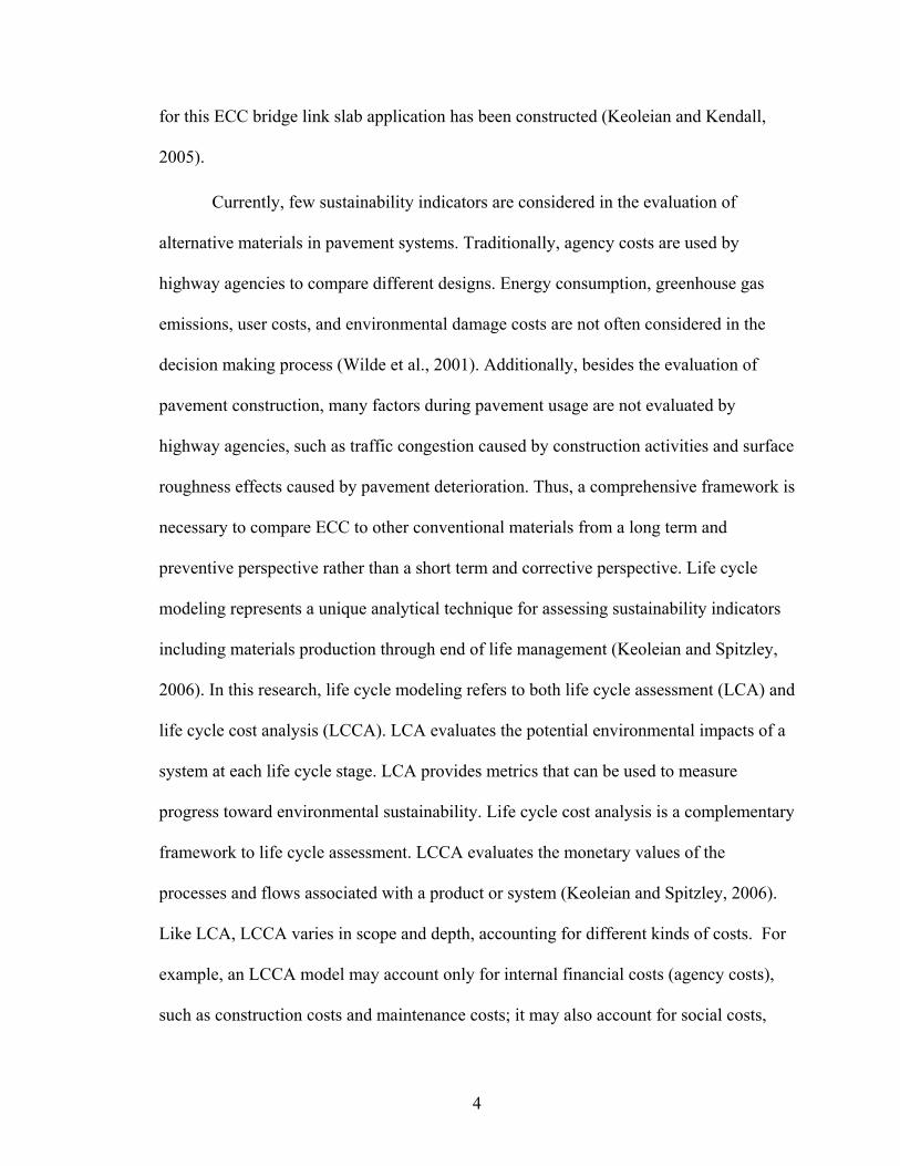
framework that takes into account environmental, economic, and social indicators. Figure
1.1 illustrates the range of sustainability issues considered in this research. Overall
sustainability which is illustrated as the shadow area in the center of Figure 1.1 requires
meeting environmental, economic, and social goals simultaneously.
EnvironmentalEnergy consumptionMaterial consumptionPollution emissionsGreenhous gasemissions
SocialUser time delay
Vehicle DamageSafety
EconomicLife cycle cost
TaxSubsidyBudget
OverallSustainability
Figure 1.1 Various sustainability issues captured in pavement systems
As a part of National Science Foundation Material Use: Science, Engineering and
Society (NSF MUSES) sustainable concrete infrastructure project, a sustainable design
framework is developed that encompasses multi-scale boundaries ranging from micro-
scale material development to macro-scale system application. Traditionally, material
scientists and engineers have focused on a limited set of performance criteria in design
3
activities within the material development process, while industrial ecologists and
economists have maintained a macro-level perspective for analyzing the life cycle
impacts at the infrastructure systems level. The sustainable design framework helps
ensure regular flows of information between these two processes. Alternative materials
designed in the material development process are translated into life cycle inventory
inputs for life cycle analysis of an infrastructure system. An aggregated set of social,
environmental, and economic indicators are derived for the infrastructure system from
material resource extraction to end of life management. These sustainability indicators
can be used to guide changes in material design in order to optimize system performance.
This design, evaluation, and re-design sequence can be repeated until more sustainable
solutions are reached.
The multi-scale design process begins with the development of a unique fiber-
reinforced material, Engineered Cementitious Composites (ECC) using a microstructural
design technique guided by micromechanical principles. Experimental testing of ECC
pavement reveals significant improvements in load carrying capacity and system ductility
compared to concrete or steel fiber reinforced concrete overlays (Qian, 2007). Thereby,
ECC can eliminate common overlay system failures such as reflective cracking (Li,
2003). ECC is a promising candidate material for road repairs, pipeline systems, and
bridge deck rehabilitation. A demonstration bridge project was recently constructed in the
fall of 2005 to provide performance data on ECC field applications. In this demonstration
project, an ECC link slab was applied to substitute for a conventional steel expansion
joint between two steel reinforced concrete bridge decks. The project site is Grove Street
over Interstate 94 (S02 of 81063) in Ypsilanti, Michigan. A life cycle assessment model
4
for this ECC bridge link slab application has been constructed (Keoleian and Kendall,
2005).
Currently, few sustainability indicators are considered in the evaluation of
alternative materials in pavement systems. Traditionally, agency costs are used by
highway agencies to compare different designs. Energy consumption, greenhouse gas
emissions, user costs, and environmental damage costs are not often considered in the
decision making process (Wilde et al., 2001). Additionally, besides the evaluation of
pavement construction, many factors during pavement usage are not evaluated by
highway agencies, such as traffic congestion caused by construction activities and surface
roughness effects caused by pavement deterioration. Thus, a comprehensive framework is
necessary to compare ECC to other conventional materials from a long term and
preventive perspective rather than a short term and corrective perspective. Life cycle
modeling represents a unique analytical technique for assessing sustainability indicators
including materials production through end of life management (Keoleian and Spitzley,
2006). In this research, life cycle modeling refers to both life cycle assessment (LCA) and
life cycle cost analysis (LCCA). LCA evaluates the potential environmental impacts of a
system at each life cycle stage. LCA provides metrics that can be used to measure
progress toward environmental sustainability. Life cycle cost analysis is a complementary
framework to life cycle assessment. LCCA evaluates the monetary values of the
processes and flows associated with a product or system (Keoleian and Spitzley, 2006).
Like LCA, LCCA varies in scope and depth, accounting for different kinds of costs. For
example, an LCCA model may account only for internal financial costs (agency costs),
such as construction costs and maintenance costs; it may also account for social costs,

5
such as user costs which are incurred by motorists who are delayed or detoured by
construction related traffic, or environmental costs including environmental damage costs
associated with construction events. In this research, LCA and LCCA methods are
coupled into an integrated LCA-LCCA model in a single computer-based model to
evaluate the life cycle of a pavement system.
While LCA and LCCA methods define and evaluate the sustainability
performance, these methods have limited management capabilities to optimize those
indicators. A pavement segment or a pavement network can be preserved through a
variety of different maintenance and rehabilitation methods and frequencies, which will
lead to different long term outcomes for life cycle energy consumption, environmental
impacts, and costs. A pavement asset management system (PAMS) is necessary, which
allows highway agencies to explore alternative pavement materials, predict pavement
deterioration over time, and select optimal preservation strategies based on specific
objectives and constraints. There are two major administrative levels of any pavement
asset management system: network-level PAMS and project-level PAMS (Mbwana,
2001). Project-level PAMS is intended to predict the pavement deterioration, select the
appropriate preservation activity, and develop the optimal preservation schedule for a
specific pavement segment. Network-level PAMS determines the pavement segment
preservation priority and budget allocation strategy. Network-level PAMS policy will
guide project-level PAMS to ensure that each individual pavement segment preservation
strategy will result in an overall optimal solution for the entire pavement network.
A number of researchers and practitioners have applied mathematical models to
pavement asset management. However, besides the economic costs, those studies do not

6
consider other sustainability indicators (e.g., energy consumption and greenhouse gas
emissions) in PAMS. Using dynamic programming, a life cycle optimization model can
mathematically determine an optimal preservation strategy to minimize the energy
consumption, environmental impacts, and costs associated with all stages of a pavement
system life cycle.
The body of literature addressing the relationship between pavement preservation
strategy, policy making, and economic factors is very limited. Multi-objective and multi-
constraint optimization methods provide a quantitative base for pavement preservation
policy making. Using the concept of Pareto efficiency, multi-objective optimization
enables highway agencies to develop their preservation strategy based on weighted
objectives to achieve maximized benefit. Multi-constraint optimization studies the impact
of agency budget constraints on user cost and total life cycle cost. The influence of fuel
taxes and government subsidies on financing a pavement system can be evaluated and
specific policy recommendations can be informed.
Due to budget constraints, highway agencies cannot preserve their entire
pavement network using the optimal preservation strategy identified by a project-level
life cycle optimization model. Thus, a priority selection model is necessary to adjust the
optimal preservation strategy and allocate the limited budget to the specific pavement
segments to achieve the global optimal result. Three priority selection methods are
developed based on benefit, benefit cost ratio, and binary integer programming.
Another challenge in developing a pavement asset management system is the
ability of managing and analyzing the large pavement condition dataset. A pavement
asset management system relies on pavement condition information for identifying

7
pavement construction sections, developing the preservation strategy, and allocating the
budget. Geographic information system (GIS), with its spatial analysis capability, allows
highway agencies to integrate, manage, query, and visualize pavement conditions. A GIS
model integrated with a pavement asset management system provides a unique way to
immediately retrieve and visualize important pavement network attributes, such as
pavement condition, current pavement preservation activity, and costs, on the graphical
map. This new framework is expected to improve the decision making process involved
in managing pavement networks.
1.2 Research Objectives
The objective of this research is to develop a comprehensive pavement
development framework to evaluate the impacts of different construction material
applications, manage a pavement network, and allocate limited budget. This framework
will be utilized to improve pavement design and preservation to ensure optimal
performance. The specific research activities include:
(1) To develop an integrated LCA-LCCA model for unbonded concrete, hot
mixed asphalt, and ECC pavement overlay systems to dynamically capture the
impacts of users, construction, and overlay deterioration.
(2) To develop a project-level pavement asset management system using life
cycle optimization method to determine the optimal preservation strategy for
pavement overlay systems.
8
(3) To investigate highway policy and enhance transportation infrastructure
sustainability using multi-objective and multi-constraint optimization methods.
(4) To develop a network-level pavement asset management system including a
priority selection model and a GIS model to allocate limited budget efficiently
and preserve a healthy pavement network while minimizing sustainability
indicators.
Fulfillment of these objectives will provide a comprehensive understanding of the
impacts and the relationship of material consumption, traffic congestion, pavement
surface deterioration, and preservation strategy in managing pavement systems. In
summary, this dissertation provides a framework and the tools that can enhance
infrastructure sustainability for pavement material selection, pavement design, and
pavement asset management.
1.3 Organization
This dissertation is presented in a multiple manuscript format. Chapter 2, 3, 4, and
5 are written as individual research papers, including the abstract, the main body and the
references.
Chapter 2 develops and presents an integrated life cycle assessment and life cycle
cost analysis model to evaluate the energy consumption, environmental impacts, and
costs of pavement overlay systems resulting from material production and distribution,
overlay construction and maintenance, construction-related traffic congestion, overlay
usage, and end of life management. A conventional unbonded concrete overlay system, a

9
hot mixed asphalt overlay system, and an alternative Engineered Cementitious
Composites (ECC) overlay system are evaluated. Material consumption, traffic
congestion caused by construction activities, and roughness effects caused by overlay
deterioration are three dominant factors that influence the environmental impacts and
costs of overlay systems. A sensitivity analysis is conducted to study the impact of traffic
growth and fuel economy improvement (Zhang et al., 2008 and Zhang et al., 2009). The
sustainability indicators presented in Chapter 2 provide a quantitative basis for the
analysis of following chapters.
Chapter 3 presents the project-level pavement asset management system. A life
cycle optimization model is developed to determine the optimal preservation strategy for
a single pavement overlay segment which minimizes total life cycle energy consumption,
greenhouse gas emissions, and costs within an analysis period. Using dynamic
programming optimization techniques, the life cycle optimization model integrates life
cycle assessment and life cycle cost analysis models with an autoregressive pavement
overlay deterioration model. The project-level pavement asset management system is
applied to the conventional unbonded concrete, hot mixed asphalt, and ECC overlay
systems. The results of optimal preservation strategies are compared to current Michigan
Department of Transportation preservation strategies. The impact of traffic growth to the
optimal preservation strategies is discussed (Zhang et al., 2009).
Chapter 4 extends the analysis of a single pavement segment based on the results
of Chapter 3. Multi-constraint and multi-objective optimization is conducted to study the
impact of agency budget constraints on user costs and total life cycle cost, identify the
trade offs between energy consumption and costs, and understand the relationships
10
between material consumption, traffic congestion, and pavement roughness effects. A
Pareto optimal solution that minimizes energy and cost objectives is developed to
enhance the preservation strategies. The influence of fuel taxes and government subsidies
on a pavement system is explored and specific policy recommendations are provided
(Zhang et al., 2008).
Chapter 5 develops a network-level pavement asset management system to
minimize environmental and economic sustainability indicators for the entire pavement
network. Life cycle assessment, life cycle cost analysis, life cycle optimization, and
project-level pavement asset management models are incorporated in the network-level
pavement asset management system. A priority selection model is implemented to
allocate a limited agency budget efficiently. A GIS model is developed to enhance the
network-level pavement asset management system by collecting, managing, and
visualizing pavement condition data. Query analysis is conducted in the GIS model to
identify the specific pavement network in the basic digital map. Linear referencing and
dynamic segmentation methods are applied to define the pavement segment and associate
pavement information with any pavement portion (Zhang et al., 2009).
Chapter 6 draws the conclusions and summarizes the original contributions of the
dissertation. Several topics are also proposed for future research.

11
References
American Society of Civil Engineering (ASCE). (2006). Road to Infrastructure Renewal—A Voter’s Guide. Reston, Va.
Li, V.C. (2003). “Durable overlay systems with engineered cementitious composites (ECC).” International Journal for Restoration of Buildings and Monuments, 9(2), 1-20.
Qian, S.Z. (2007). “Influence of Concrete Material Ductility on the Behavior of High Stress Concentration Zones.” Doctoral thesis. University of Michigan, Ann Arbor, Michigan.
Keoleian, G. A. and Spitzley, D.V. (2006). “Life Cycle Based Sustainability Metrics.” Chapter 7 in Sustainability Science and Engineering: Defining Principles (Sustainability Science and Engineering, Volume 1), M.A. Abraham, Ed. Elsevier, pp. 127-159.
Keoleian, G. A. and Kendall, A. (2005). “Life cycle modeling of concrete bridge design: Comparison of engineered cementitious composite link slabs and conventional steel expansion joints.” Journal of Infrastructure Systems, 11(1), 51-60.
Mbwana, J. R. (2001). “A framework for developing stochastic multi-objective pavement management system.” Technology Transfer in Road Transportation in Africa, Arusha, Tanzania.
Zhang, H., Keoleian, G. A., and Lepech, M. D. (2008). “An integrated life cycle assessment and life cycle analysis model for pavement overlay systems.” First International Symposium on Life-Cycle Civil Engineering, Varenna, Italy, pp. 907-915.
Zhang, H., Keoleian, G. A., and Lepech, M. D. (2008). “Multi-objective and Multi-constraint optimization in project-level pavement asset management.” Transportation Research Part A: Policy and Practice. Submitted.
Zhang, H., Lepech, M. D., Keoleian, G. A., Qian, S. Z., and Li, V. C. (2009). “Dynamic life cycle modeling of pavement overlay systems: capturing the impacts of users, construction, and roadway deterioration.” To be submitted to Journal of Infrastructure Systems.
Zhang, H., Keoleian, G. A., and Lepech, M. D. (2009). “Life cycle optimization of pavement overlay systems.” To be submitted to Journal of Infrastructure Systems.

12
Zhang, H., Keoleian, G. A., and Lepech, M. D. (2009). “Network-level pavement asset management system integrated with life cycle analysis and life cycle optimization.” To be submitted to Transportation Research Part B: Methodological.
Wilde, W. J., Waalkes, S., and Harrison, R. (2001). Life cycle cost analysis of Portland cement concrete pavement, University of Texas at Austin, Austin, Texas.
13
CHAPTER 2
INTEGRATED LIFE CYCLE ASSESSMENT AND LIFE CYCLE COST ANALYSIS MODEL
ABSTRACT
Pavement systems have significant impacts on environment, economy, and
society due to large material consumption, energy input, and capital investment. To
evaluate the sustainability of pavement systems, an integrated life cycle assessment and
life cycle cost analysis model was developed to calculate the energy consumption,
environmental impacts and costs of pavement overlay systems resulting from material
production and distribution, overlay construction and maintenance, construction-related
traffic congestion, overlay usage, and end of life management. An unbonded concrete
overlay system, a hot mixed asphalt overlay system, and an alternative engineered
cementitious composite (ECC) overlay system are examined. Model results indicate that
the ECC overlay system significantly reduces total life cycle energy consumption,
greenhouse gas (GHG) emissions, and economic costs compared to conventional overlay
systems. These advantages are derived from the enhanced material properties of ECC
which prevent reflective cracking failures. Material consumption, traffic congestion, and
pavement surface roughness effects are identified as three dominant factors that increase
both the environmental impacts and the cost of overlay systems.

14
2.1 Introduction
Pavement systems are fundamental components of our automobile transportation
systems. While the transportation of people and goods is increasing rapidly, pavement
systems have serious impacts on the environment and the economy. Yet, the American
Society of Civil Engineers (ASCE) report card assigns US roads a grade of D (poor
condition). This poor road condition costs US motorists an estimated $54 billion annually
in vehicle repair and operating costs (ASCE, 2006).
As the pavements age and deteriorate, preservation (maintenance and
rehabilitation) are required to provide a high level of safety and service (Huang, 2004).
For pavements subjected to heavy traffic, one of the most prevalent preservation
strategies is the placement of an overlay on top of the existing pavement (DOT, 1989).
An overlay provides protection to the pavement structure, reduces the rate of pavement
deterioration, corrects surface deficiencies, and adds some strength to the existing
pavement structure. Depending on the type of overlay and existing pavement, two
possible designs are generally used: an unbonded concrete overlay or a hot mixed asphalt
(HMA) overlay. An unbonded concrete overlay is typically placed over a pavement
which is badly cracked. A separation layer, usually consisting of asphalt less than 50 mm
thick, is placed between the new concrete overlay and the cleaned existing pavement to
prevent reflective cracking (ACPA, 1990). An HMA overlay usually has several layers
with the different mixes of hot mixed asphalt (Huang, 2004). Concrete and asphalt are the
most common materials used in the construction of pavement and overlay systems.
Nearly 57% of the mileage of interstate highways and other freeways is either concrete
surface or concrete base, while other highways, rural roads, or urban streets are asphalt
15
surface (Zapata, 2005). The use of both concrete and asphalt pose significant
environmental challenges. The world wide production of cement, a key constituent in
concrete, releases more than 1.6 billion metric tons of CO2 annually, accounting for over
8% of total CO2 emissions from all human activities (Wilson, 1993), and significant
levels of other pollutants, such as particulate matter and sulfur oxides (Estakhri and
Saylak, 2005). Asphalt, a petroleum byproduct, is energy intensive and contains 7,354
MJ of feedstock energy per cubic meter (Zapata, 2005). Asphalt is also a large source of
volatile organic compounds (VOC) accounting for 200,000 metric ton of VOC emissions
each year in the U.S. from asphalt pavement construction (Spivey, 2000). Additionally,
concrete and asphalt have some physical limitations that contribute to durability concerns,
which increase the likelihood of pavement failure and maintenance frequency.
Consequently, alternative materials are being developed to improve road performance.
Part of the process to introduce new materials into field application includes evaluation of
the environmental impacts at each stage of the material life cycle from resource
extraction through manufacturing, transportation, construction and final disposal.
Additionally, sustainability is increasingly adopted as a framework for designing and
constructing pavement systems. Life cycle assessment (LCA) and life cycle cost analysis
(LCCA) methodologies provide the means for evaluating the sustainability of pavement
systems.
LCA is an analytical technique for assessing potential environmental burdens and
impacts. LCA provides metrics that can be used to measure progress toward
environmental sustainability (Keoleian and Spitzley, 2006). LCA studies the
environmental aspects and potential impacts throughout a product’s life from raw

16
material acquisition through production, use and disposal (ISO, 1997). LCCA evaluates
the monetary values of processes and flows associated with a product or system
(Keoleian and Spitzley, 2006). Like LCA models, LCCA models vary in scope and depth,
accounting for different kinds of costs. For example, LCCA models may account only
for internal costs (agency costs), such as construction costs and maintenance costs; it may
also account for social costs, such as user costs which are incurred by motorists who are
delayed or detoured by construction related traffic, or environmental costs including
environmental damage costs associated with construction events.
Two approaches have been used in previous LCA and LCCA studies. One
approach uses a process level LCA method to trace the energy consumption and related
environmental impact of the system (Zapata, 2005). The other approach is the economic
input-output analysis-based life cycle analysis (EIO-LCA) method, developed by
Carnegie Mellon University’s Green Design Initiative. This method traces the various
economic transactions for various sectors and uses an economic input-output matrix of
the US economy to evaluate resource requirements and environmental emissions
(Horvath and Hendrickson, 1998).
Only a few efforts on pavement life cycle modeling have been made. The
Swedish Environmental Research Institute (IVL) conducted a life cycle assessment of
concrete and asphalt pavements based on process flows, including pavement construction,
maintenance and operation (Stripple, 2001). Additionally, the University of Texas Center
for Transportation Research performed a life cycle cost assessment which is an
engineering-economic analysis tool used to quantify the differential costs of alternative
investment options for a given project, to evaluate concrete pavement (Wilde et al., 2001).
17
Horvath and Hendrickson used the EIO-LCA model to study the environmental impacts
of asphalt and steel-reinforced concrete pavements. However, these studies did not
analyze the maintenance procedures and their effects on extending the pavement service
life and did not capture the effects of the pavement deterioration on vehicles.
An integrated LCA and LCCA model (LCA-LCCA) was developed and applied
to compare the energy consumption, environmental impacts, and costs for an overlay
system built using concrete, HMA, or a new material—Engineered Cementitious
Composites (ECC), an ultra ductile form of concrete.
ECC is a unique fiber-reinforced composite developed using a microstructural
design technique guided by micromechanical principles. ECC is deliberately designed as
a fiber reinforced cementitious material with a deformation behavior analogous to that of
metals (Li and Fischer, 2002). Experimental testing of ECC overlays reveal significant
improvements in load carrying capacity and system ductility compared to concrete or
steel fiber reinforced concrete overlays (Qian, 2007). Thereby, ECC can eliminate
common overlay system failures such as reflective cracking (Li, 2003). Since the
introduction of this material a decade ago, ECC has undergone a major evolution both in
the academic and industrial communities (Li, 2002). ECC is a promising candidate
material for road repairs, pavement overlays (Li, 2003), and bridge deck rehabilitation
(Gilani, 2001). A demonstration bridge project was constructed in the fall of 2005 to
provide performance data on ECC field applications. In this demonstration project, an
ECC link slab was applied to substitute the conventional steel expansion joint between
two steel reinforced concrete bridge decks. The project site is Grove Street over Interstate

18
94 (S02 of 81063) in Ypsilanti, Michigan. An LCA model for this ECC bridge link slab
application has been constructed (Keoleian and Kendall, 2005).
The objective of this chapter is to create a model that can analytically measure the
sustainability performance of pavement overlay systems. In addition, pavement
construction and preservation, roadway deterioration, and the impacts of traffic are
dynamically captured. This integrated model is unique in its ability to evaluate pavement
overlay life cycle energy consumption, environmental impacts, and costs including the
upstream burdens of materials and fuel production. In the following section, the system
boundary is defined and the integrated LCA-LCCA models are described. Subsequently,
the life cycle model is applied to compare the energy consumption, environmental
impacts, and the costs of three pavement overlay systems. Finally, sensitivity analysis is
performed for different traffic growth and fuel economy improvement scenarios.
2.2 Methodology
2.2.1 System Definition
The overlay designs analyzed in this study are constructed upon an existing
reinforced concrete pavement originally built by the Michigan Department of
Transportation (MDOT). The three overlay systems are modeled as 10 km long and four
lanes wide (two lanes in each direction). Figure 2.1 illustrates the structures of the
different types of the overlay systems in one direction including the thickness of different
layers. The thickness of the overlay depends on the material and construction methods.
These pavement overlay designs are based on the results from an experimental study
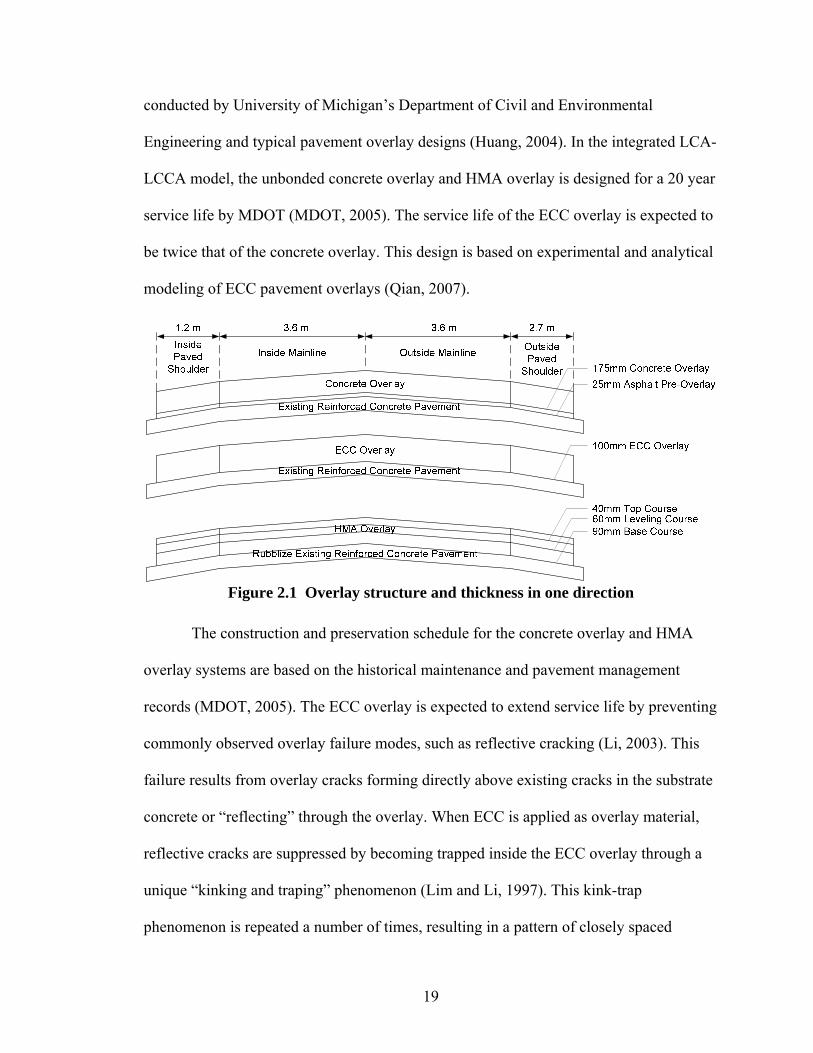
19
conducted by University of Michigan’s Department of Civil and Environmental
Engineering and typical pavement overlay designs (Huang, 2004). In the integrated LCA-
LCCA model, the unbonded concrete overlay and HMA overlay is designed for a 20 year
service life by MDOT (MDOT, 2005). The service life of the ECC overlay is expected to
be twice that of the concrete overlay. This design is based on experimental and analytical
modeling of ECC pavement overlays (Qian, 2007).
Figure 2.1 Overlay structure and thickness in one direction
The construction and preservation schedule for the concrete overlay and HMA
overlay systems are based on the historical maintenance and pavement management
records (MDOT, 2005). The ECC overlay is expected to extend service life by preventing
commonly observed overlay failure modes, such as reflective cracking (Li, 2003). This
failure results from overlay cracks forming directly above existing cracks in the substrate
concrete or “reflecting” through the overlay. When ECC is applied as overlay material,
reflective cracks are suppressed by becoming trapped inside the ECC overlay through a
unique “kinking and traping” phenomenon (Lim and Li, 1997). This kink-trap
phenomenon is repeated a number of times, resulting in a pattern of closely spaced
20
microcracks, effectively eliminating reflective cracking and surface failure modes (Li,
2003). Thus, ECC overlays can achieve a longer life with a much thinner thickness
compared with concrete. In addition, maintenance frequency and maintenance material
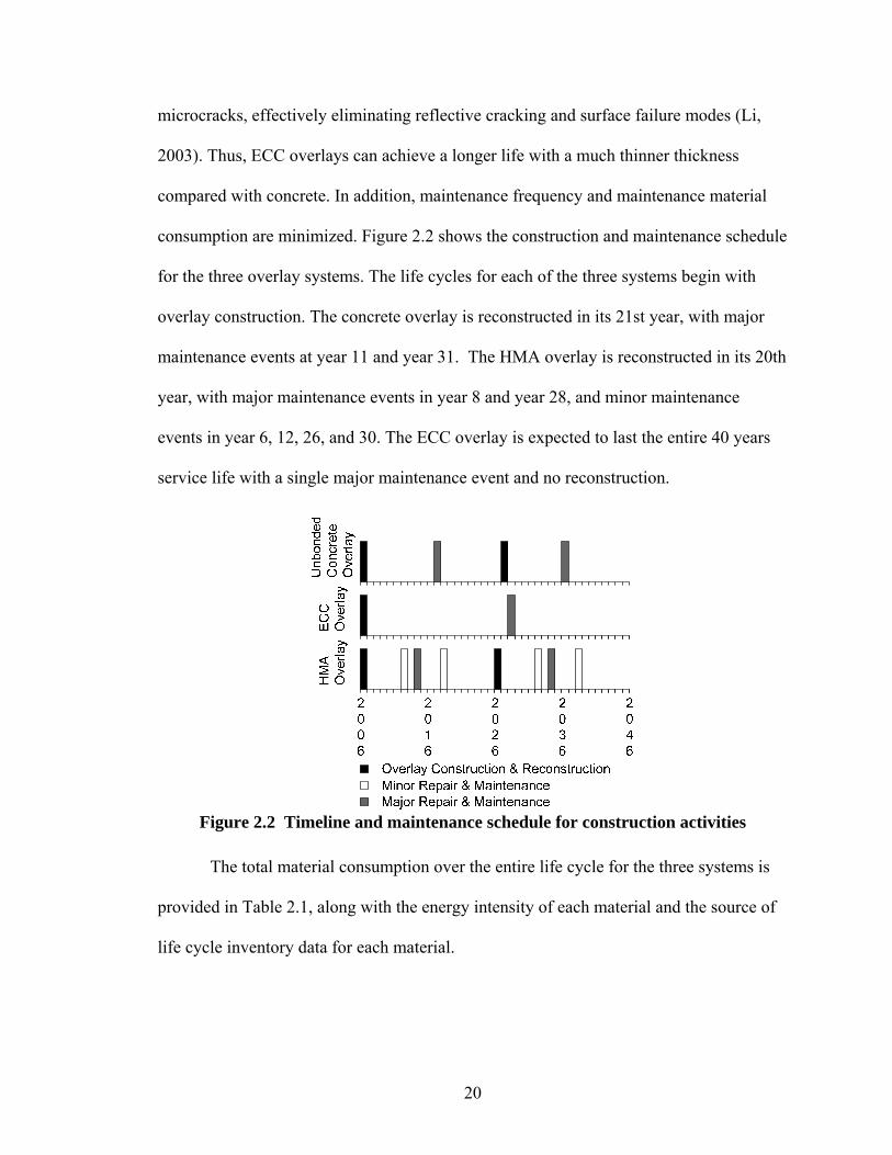
consumption are minimized. Figure 2.2 shows the construction and maintenance schedule
for the three overlay systems. The life cycles for each of the three systems begin with
overlay construction. The concrete overlay is reconstructed in its 21st year, with major
maintenance events at year 11 and year 31. The HMA overlay is reconstructed in its 20th
year, with major maintenance events in year 8 and year 28, and minor maintenance
events in year 6, 12, 26, and 30. The ECC overlay is expected to last the entire 40 years
service life with a single major maintenance event and no reconstruction.
Figure 2.2 Timeline and maintenance schedule for construction activities
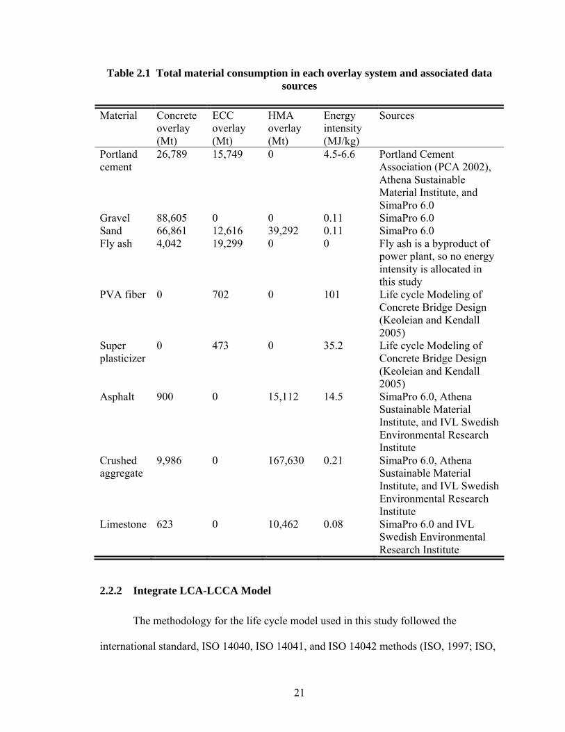
The total material consumption over the entire life cycle for the three systems is
provided in Table 2.1, along with the energy intensity of each material and the source of
life cycle inventory data for each material.
21
Table 2.1 Total material consumption in each overlay system and associated data sources
Material Concrete
overlay (Mt)
ECC overlay (Mt)
HMA overlay (Mt)
Energy intensity (MJ/kg)
Sources
Portland cement
26,789 15,749 0 4.5-6.6 Portland Cement Association (PCA 2002), Athena Sustainable Material Institute, and SimaPro 6.0
Gravel 88,605 0 0 0.11 SimaPro 6.0 Sand 66,861 12,616 39,292 0.11 SimaPro 6.0 Fly ash 4,042 19,299 0 0 Fly ash is a byproduct of
power plant, so no energy intensity is allocated in this study
PVA fiber 0 702 0 101 Life cycle Modeling of Concrete Bridge Design (Keoleian and Kendall 2005)
Super plasticizer
0 473 0 35.2 Life cycle Modeling of Concrete Bridge Design (Keoleian and Kendall 2005)
Asphalt 900 0 15,112 14.5 SimaPro 6.0, Athena Sustainable Material Institute, and IVL Swedish Environmental Research Institute
Crushed aggregate
9,986 0 167,630 0.21 SimaPro 6.0, Athena Sustainable Material Institute, and IVL Swedish Environmental Research Institute
Limestone 623 0 10,462 0.08 SimaPro 6.0 and IVL Swedish Environmental Research Institute
2.2.2 Integrate LCA-LCCA Model
The methodology for the life cycle model used in this study followed the
international standard, ISO 14040, ISO 14041, and ISO 14042 methods (ISO, 1997; ISO,

22
1998; ISO, 2000). The complete integrated LCA-LCCA model framework, including
modules which make up the model, is shown in Figure 2.3.
Life Cycle Assessment Model
Life Cycle Cost Assessment Model
Model Parameters
User Input and System Definition
Environmental Sustainable Indicators
Material Module
Construction Module
Distribution Module
Congestion Module
Usage Module
End of Life Module
Agency Costs Social Costs
-Construction-Maintenance-EOL
User Cost-User time delay-Vehicle damage
Environmental Cost-Agency activity emissions-Vehicle emissions
SimaPro Model NONROAD Emissions Model
MOBILE 6.2 Emissions Model
KyUCP Traffic Flow Model
Figure 2.3 Integrated LCA-LCCA model framework
2.2.2.1 Life Cycle Assessment Model
The LCA model quantifies the environmental and social performance of an
overlay system throughout its life cycle, from raw material acquisition to final disposal or
recycling. The LCA model is divided into six modules: material production, consisting of
the acquisition and processing of raw materials; construction, including all construction
processes, maintenance activities, and related construction machine usage; distribution,
accounting for transport of materials and equipment to and from the construction site;
traffic congestion, which models all construction and maintenance related traffic
congestion; usage, including overlay roughness effects on vehicular travel and fuel

23
consumption during normal traffic flow; and end of life, which models demolition of the
overlay and processing of the materials.
The material production module is modeled using data sets from various sources,
including the Portland Cement Association, the Athena Sustainable Materials Institute,
and the SimaPro 6.0 life cycle data base. The modeled material compositions of concrete,
HMA, and ECC are shown in Figure 2.4.
0% 20% 40% 60% 80% 100%
Concrete
ECC
HMA
CementPVA FiberSuperplasticizerGravelBitumenSandLimestoneWaterFly Ash
Figure 2.4 Material composition of concrete, HMA, and ECC materials
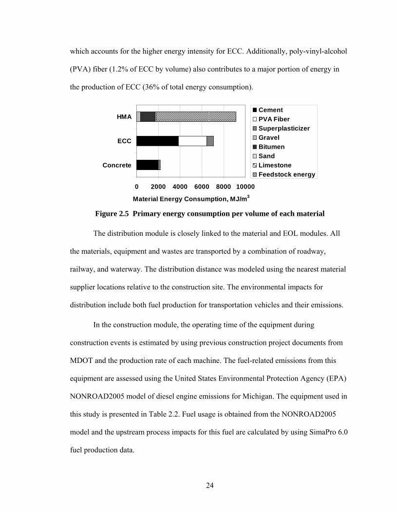
The total primary energy contribution per volume for each material constituent is
shown in Figure 2.5. The unit volume primary energy consumption for concrete, ECC,
and HMA is 2,212, 7,103, and 9,142 MJ/m3, respectively. In the case of HMA, although
the asphalt is only 6.5% of HMA by volume, the feedstock energy (7,353 MJ/m3 HMA)
contained in the asphalt binder accounts for 80% of the total energy consumed in HMA
production. In comparing ECC and concrete, ECC contains a large amount of fly ash
(33.9% of ECC by volume compared to 2.1% of concrete), which is a byproduct of coal
consumption. Consequently, there is no environmental burden or energy consumption
allocated to this substitute. However, the particular ECC mix used in this study contains
twice as much cement per volume compared to concrete (27.7% compared to 13.7%),
24
which accounts for the higher energy intensity for ECC. Additionally, poly-vinyl-alcohol
(PVA) fiber (1.2% of ECC by volume) also contributes to a major portion of energy in
the production of ECC (36% of total energy consumption).
0 2000 4000 6000 8000 10000
Concrete
ECC
HMA
Material Energy Consumption, MJ/m3
CementPVA FiberSuperplasticizerGravelBitumenSandLimestoneFeedstock energy
Figure 2.5 Primary energy consumption per volume of each material
The distribution module is closely linked to the material and EOL modules. All
the materials, equipment and wastes are transported by a combination of roadway,
railway, and waterway. The distribution distance was modeled using the nearest material
supplier locations relative to the construction site. The environmental impacts for
distribution include both fuel production for transportation vehicles and their emissions.
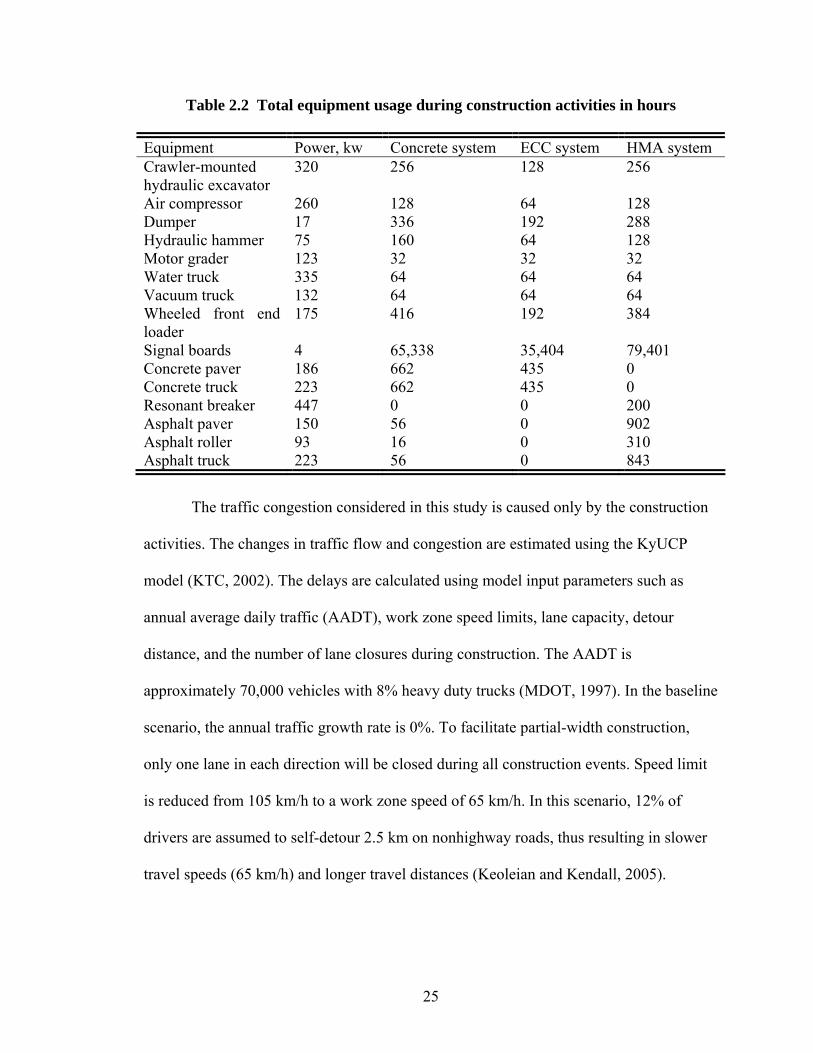
In the construction module, the operating time of the equipment during
construction events is estimated by using previous construction project documents from
MDOT and the production rate of each machine. The fuel-related emissions from this
equipment are assessed using the United States Environmental Protection Agency (EPA)
NONROAD2005 model of diesel engine emissions for Michigan. The equipment used in
this study is presented in Table 2.2. Fuel usage is obtained from the NONROAD2005
model and the upstream process impacts for this fuel are calculated by using SimaPro 6.0
fuel production data.
25
Table 2.2 Total equipment usage during construction activities in hours Equipment Power, kw Concrete system ECC system HMA system Crawler-mounted hydraulic excavator
320 256 128 256
Air compressor 260 128 64 128 Dumper 17 336 192 288 Hydraulic hammer 75 160 64 128 Motor grader 123 32 32 32 Water truck 335 64 64 64 Vacuum truck 132 64 64 64 Wheeled front end loader
175 416 192 384
Signal boards 4 65,338 35,404 79,401 Concrete paver 186 662 435 0 Concrete truck 223 662 435 0 Resonant breaker 447 0 0 200 Asphalt paver 150 56 0 902 Asphalt roller 93 16 0 310 Asphalt truck 223 56 0 843
The traffic congestion considered in this study is caused only by the construction
activities. The changes in traffic flow and congestion are estimated using the KyUCP
model (KTC, 2002). The delays are calculated using model input parameters such as
annual average daily traffic (AADT), work zone speed limits, lane capacity, detour
distance, and the number of lane closures during construction. The AADT is
approximately 70,000 vehicles with 8% heavy duty trucks (MDOT, 1997). In the baseline
scenario, the annual traffic growth rate is 0%. To facilitate partial-width construction,
only one lane in each direction will be closed during all construction events. Speed limit
is reduced from 105 km/h to a work zone speed of 65 km/h. In this scenario, 12% of
drivers are assumed to self-detour 2.5 km on nonhighway roads, thus resulting in slower
travel speeds (65 km/h) and longer travel distances (Keoleian and Kendall, 2005).

26
Once vehicle delay and congestion due to construction and preservation events
are calculated, these results are coupled with fuel consumption and vehicle emissions to
measure environmental impacts. Fuel consumption is determined using fuel economy
estimated by city and highway drive cycles. The city drive cycle is used to estimate the
fuel consumption during congestion and detour modes. Likewise, the highway drive
cycle is used to model the normal traffic flow during free flowing traffic periods. Fuel
consumption for passenger cars, light duty vehicles and heavy duty vehicles is taken from
the Vision Model, developed by US Department of Energy (DOE) Center for
Transportation Research at Argonne National Laboratory (DOE, 2004). Carbon dioxide
(CO2) emissions are derived using fuel consumption, carbon content, and engine
efficiency. Other vehicle emissions are calculated using USEPA’s MOBILE 6.2 software
at varying traffic speeds. MOBILE 6.2 is used to predict the tailpipe emissions and
evaporative emissions on a per year basis through 2050. Four localized MOBILE 6.2 data
inputs for the winter and summer seasons used in this study include annually temperature
range, Reid vapor pressure, age distribution of the vehicle fleet, and average vehicle
miles traveled data (SEMCOG, 2006). The output results of fuel consumption and vehicle
emissions in the LCA model are calculated using Equation 2.1 based on the difference
between traffic flow during construction periods and traffic flow during normal
conditions. xVMT represents the total vehicle miles traveled under normal, highway,
work zone, detour, and queue conditions. xY represents the marginal change for different
environmental indicators, such as emission values (g/km) and fuel usage (L/km).
* * * * *Total Highway Highway Queue Queue Work zone Workzone Detour Detour Normal NormalY VMT Y VMT Y VMT Y VMT Y VMT Y= + + + − (2.1)

27
For pavement infrastructure with a long service life cycle, the output results are
highly dependent on future changes in fuel economy and annual traffic growth rate. This
effect will be discussed in the scenario analysis section.
The traffic congestion module predicts how construction activities affect traffic
flow and emissions. The usage module describes the effects on traffic during normal
operation of the overlay section, and this module is significantly more complex than the
other modules. There are two primary factors which affect fuel consumption and vehicle
emissions: fuel economy changes and pavement roughness changes over time.
In this model, the fuel economy of a heavy duty truck combining cost-effective
conventional improvements with hybridization is predicted to save 32% of total energy
consumption over a 20 year period (Langer, 2004). This is described by Equation 2.2.
*(1 )nn baseFE FE r= + (2.2)
nFE is the heavy duty truck fuel economy factor for nth year and baseFE is the 2003
baseline heavy duty truck fuel economy factor which is presented in the Vision model.
The value r is the annual fuel economy improvement, estimated at 1.5% fuel
consumption savings per year due to increased boosting, improved combustion control
and other design changes.
For passenger cars and other light duty vehicles, there are two methods to
estimate future fuel economy trends. The first method is also described by Equation 2.2.
In this case, baseFE is the 2003 baseline car and light duty vehicle fuel economy factor
based on the data from the Transportation Energy Data Book developed by the DOE
Center for Transportation Analysis (Davis and Diegel, 2002 ). The value r is estimated

28
at 1% fuel consumption savings per year (Davis and Diegel, 2002), based on fuel
economy trends from 1995-2005. The second method is based on a model of future
performance of the internal combustion engine (ICE) over a 30 year time horizon
(Heywood et al., 2004) shown as Equation 2.3. The time period is extrapolated to 40
years to match the service life of the three overlay system. In this equation, 0n and n are
the initial year and the nth year of this project, respectively.
4 3 2 2 1 10 0 04.96 10 ( ) 4.08 10 ( ) 2.28 10 ( ) 1.88 10n baseFE n n n n n n FE− − − −= − × × − + × × − − × × − + × +
(2.3)
Due to surface deterioration, the overlay surface roughness increases continuously
over time. Roughness is generally defined as an expression of road surface irregularity
which affects the operation of a vehicle, including speed of travel, fuel economy,
emissions and safety. Hence, it also impacts vehicle operation costs and maintenance
costs. Roughness is often measured using the international roughness index (IRI), which
was developed by the World Bank in the 1980s (Sayers et al., 1986). The IRI is a ratio of
a standard vehicle’s accumulated suspension motion (in mm, inches, etc.) divided by
vehicle distance traveled during the measurement (km, mi, etc.). The commonly
recommended unit of IRI is meters per kilometer (m/km) (Sayers and Karamihas, 1995).
The IRI describes a linear scale of roughness beginning with 0 m/km for a perfectly flat
surface and no theoretical upper limit, although IRI values above 8 m/km means driving
uncomfortably and reducing the speed. (Archondo-Callao, 1999).
The pavement performance of the concrete and HMA overlays was predicted by
MDOT based on empirical data (MDOT, 2005). By suppressing reflective cracking, the
pavement performance of the ECC overlay is much better than the concrete overlay (Qian,

29
2007). To gauge pavement conditions in Michigan, a Distress Index (DI) is used which
represents a holistic measure of pavement condition including surface roughness and
deterioration. A set of plots showing the evolution of DI for each overlay over time is
shown in Figure 2.6. As can be seen, the distress of overlay decreases from individual
preservation activities (Figure 2.2). The DI and time relationship for each overlay can be
described by several polynomial equations.
0 10 20 30 400
10
20
30
40
50
60
Pavement age, year
Dis
tress
Inde
x
ConcreteECCHMA
Figure 2.6 Distress index of each pavement
DI and IRI have been related for the concrete and HMA overlays through
Equation 2.4 and Equation 2.5, respectively (Lee et al., 2002). For the ECC overlay, the
same equation was used as the concrete overlay.
0.3016.4435
DIIRIDI
⎛ ⎞= ⎜ ⎟−⎝ ⎠ (2.4)
0.30826.8435
DIIRIDI
⎛ ⎞= ⎜ ⎟−⎝ ⎠ (2.5)
30
Increased road roughness is estimated to reduce onroad fuel economy by 4.2%
relative to the government listed fuel economy (EPA, 2006). WesTrack has related
roadway roughness effects to the fuel consumption of heavy duty trucks at a constant
speed (WesTrack, 1999), shown in Equation 2.6.
0.0667 0.8667FCF IRI= + (2.6)
where FCF is the fuel consumption factor (greater than 1.0).
Using this fuel consumption factor, the total fuel consumption can be assessed by
multiplying the ideal fuel consumption on a perfectly smooth overlay by the FCF. The
final result is expressed as the difference between fuel consumed during vehicle operation
on a rough overlay and on a ideally smooth overlay.
To estimate the effect of roughness on emissions, both driving behavior and
engine load are considered. Most drivers slow down when driving on a rough road. The
World Bank classifies “comfortable riding conditions” as up to 80-95 km/h when the IRI
is 3.5-4.5 m/km (Archondo-Callao, 1999). The speed adjustment factor S , based on
average running speed and IRI, is described by Equation 2.7 (Wilde et al., 2001).
0.0928(0.52 0.26 )4.3065 IRIS e −= (2.7)
Roughness changes affect highway capacity due to speed reduction. Highway
capacity decreases approximately 150 passenger car units per hour per lane as IRI
increases by 1 m/km (Chandra, 2004). This lane capacity change directly determines
queue formation and detour selection, assessed through the KyUCP model.
Operating emissions for a vehicle traveling on a rough overlay versus on an
ideally smooth overlay are calculated using the speed adjustment factor and the lane
capacity change factor.

31
Another source of increased vehicle emissions is engine load changes owing to
increased friction and vertical acceleration of the vehicle body caused by additional
roughness. To estimate emissions produced by engine load change a typical torque curve
for an engine (Tunnell, 2005) was used. Within the region of maximum torque, there is
an area designated the Not-To-Exceed (NTE) zone. The EPA defines the NTE zone to
control heavy-duty engine emissions over the full range of speed and load combinations
commonly experienced during vehicle operation. Inside this zone, under the maximum
torque curve of an engine the emissions must not exceed a specified value for any of the
regulated pollutants.
Because of the constraints imposed by NTE limits, a constant emission rate (in
grams of emission per liter of fuel burned) is assumed for a typical speed of operation (90
km/h to 105 km/h) of a truck (Tunnell, 2005). Any additional emissions produced as a
result of engine load increasing can be estimated as proportional to the fuel consumption
increase calculated by Equation 2.6.
In the end of life module, all material is assumed deposited in a landfill in the
baseline scenario. The disposal materials transported from the construction site to landfill
are modeled in the same method as the distribution module.
By quantifying environmental and social impacts, the LCA model can also
provide the input data for a life cycle cost model.
2.2.2.2 Life Cycle Cost Analysis Model
The LCCA model calculates the agency, user, and environmental costs. The
framework of the LCCA model was first developed by Kendall et al (Kendall et al.,
2006).

32
Agency costs include all costs incurred directly by the highway agencies over the
lifetime of the overlay system. These are typically construction and preservation costs
including material costs, equipment rental and operating costs, and labor costs. The actual
agency costs were collected from MDOT construction contracts. Table 2.3 shows the
agency costs breakdown for the construction activities modeled.
Table 2.3 Agency costs breakdown for overlay construction activities
Construction activity Overlay type
Process Total cost, 2006 U.S. $/lane-mile
Concrete Overlay placement $170,500 ECC Overlay placement $210,800
Overlay initial construction
HMA Rubblize and overlay placement
$171,000
Concrete Replace 10% seals, crack seal any cracked slab (est 8%)
$8,000
ECC N/A N/A
Overlay minor maintenance
HMA Crack seal $6,400 Concrete Replace 30% seals, replace
15% joints, crack seal any cracked slab (est 15%)
$46,000
ECC Replace 30% seals, replace 15% joints, crack seal any cracked slab (est 15%)
$68,000
Overly major maintenance
HMA Crack seal, patch $58,000 Concrete Overlay placement $154,000 ECC N/A N/A
Overlay reconstruction
HMA Overlay placement $154,500
Social costs are not directly addressed in the construction and preservation
activities of a transportation agency. Generally, social costs include user costs and
environmental costs. User costs are more likely to be considered in more densely
populated states or urban areas, while environmental costs are not considered by any state
(Chan et al., 2006). The literature is limited in examining how social costs are actually
applied by state DOTs.
33
Overlay construction and preservation activities and overlay deterioration will
affect traffic flow. These impacts are termed user costs, since they are incurred by
highway users traveling on the system. User costs are the differential costs incurred while
driving between normal operations and work zone operations or on poor pavement
conditions. User costs are an aggregation of user delay costs, vehicle operating costs, and
risk of traffic accidents (Wilde et al, 2001).
User time delay costs normally dominate user costs. The total costs of travelers
sitting in traffic are determined by multiplying the value of time and the additional
number of hours spent in work zone congestion or on detours, compared to the number of
hours spent traveling the equivalent distance in normal traffic flow conditions. The value
of time (delay costs rate) for passenger vehicles, single unit trucks, and combination
trucks is $11.58/Veh-hr (vehicle hour), $18.54/Veh-hr, and $22.31/Veh-hr respectively,
estimated by the Federal Highway Administration (Wall and Smith, 1998). Costs are in
1996 dollars and updated to 2006 dollars in the LCCA model using the Consumer Price
Index.
Vehicle operating costs account for higher fuel consumption and thus higher fuel
costs when driving through a work zone or on a deteriorated overlay, as compared to
normal conditions. If drivers choose a detour to avoid congestion, they will travel a
greater distance and consume more fuel. Due to surface deterioration, the overlay surface
roughness increases continuously over time. Fuel costs are based on a 2006 average of
retail fuel costs in Michigan. Fuel price changes have little impact on total user costs,
since fuel accounts for less than 3% of total user costs as compared to 85% for user delay
costs.

34
The last element of user costs is based on increased risk of traffic accidents. Both
traveling through construction work zones and traveling additional distance when detours
are chosen to avoid work zone congestion contribute to increased costs of traffic
accidents. In the State of Michigan, an additional $0.13/VMT traveled in the construction
zone and a $0.09/VMT traveled in a detour are used to estimate the increased risk costs
(MDOT, 2002).
User costs should be considered when deciding the proper long term design of an
overlay system, since user costs associated with overlay construction and maintenance
usually exceed agency costs by a significant amount (Zhang et al., 2009; Wilde et al.,
2001). Minimizing the interruption of traffic flow during construction and preservation
activities over the total life cycle of an overlay is important for highway design.
Environmental costs measure the pollution damage costs over the entire life cycle
of an overlay system. These costs are related to both direct and indirect impacts to human
health from air pollution; the inhaling of air pollutants detrimental to human health, and
greenhouse gases that result in global warming. Six criteria pollutants specified by the
EPA which have direct impact on human health are considered, including sulfur oxides
(SOx), nitrogen oxides (NOx), carbon monoxide (CO), particular matter (PM2.5), lead (Pb),
and volatile organic compounds (VOC). Three major greenhouse gases that are
inventoried include carbon dioxide (CO2), methane (CH4), and nitrous oxide (N2O). The
marginal costs of these pollutants are shown in Table 2.4 (Kendall et al., 2006). Since the
criteria pollutants are sensitive to geographic region, values for urban, urban fringe and
rural areas are calculated separately. GHG emissions have global consequences, therefore
global costs are used.

35
Table 2.4 Air pollution damage costs by impacted region (Kendall et al., 2006)
Pollutant name Average cost (2006 U.S. $/Mt) Urban Urban fringe Rural Global SOx 6,732 3,013 877 NOx 171 71 21 CO 186 96 23 PM2.5 2 1 0 Pb 4,333 2,256 526 VOC 2,147 2,147 2,147 CO2 23 CH4 7,792 N2O 421
The discount rate is a central element to economic analysis and can significantly
influence LCCA results. Historical trends over the last several years indicate that the real
time value of money ranges approximately between 3% and 5% (Wilde et al., 2001). In
the LCCA model, a real discount rate is used. Real discount rates reflect the true time
value of money with no inflation premium. The real discount rate of 4% for agency and
user costs was estimated based on values recommended by the U.S. Office of
Management and Budget (OMB) (Office of Management and Budget, 2005).
Environmental costs are not discounted traditionally, due to significant
uncertainty in environmental impacts and their associated costs. A series of sliding-scale
discount rates was developed by Weitzman using a gamma discounting approach. The
discount rate was divided into following scale: for the immediate future (years 1-5), a 4%
discount rate is used; for the near future (years 6-25), a 3% discount rate is used; for the
medium future (yeas 26-75), a 2% discount rate is used (Weitzam, 2001).

36
2.3 Results and Discussions
2.3.1 Life Cycle Assessment Results
Total life cycle assessment results represent the environmental impacts from the
material module, construction module, distribution module, traffic congestion module,
usage module and EOL module over the 40 year life cycle. The environmental indicators
in this study include energy consumption, greenhouse gas emissions, air pollutant
emissions, and water pollutant emissions.
2.3.1.1 Energy consumption
Life cycle energy consumptions for 10 kilometers of the concrete overlay, ECC
overlay and HMA overlay are 6.8×10⁵ GJ, 5.8×10⁵ GJ, and 2.1×10⁶ GJ, respectively. The
life cycle energy consumption by stage is shown in Figure 2.7. The life cycle energy
consumption for three systems is dominated by material production energy, traffic
congestion related energy and roughness related energy. Roughness related energy has
not been previously studied using LCA. Without considering the roughness effect, the life
cycle energy consumptions of concrete, ECC, and HMA overlay systems will decrease
23%, 36%, and 14%, respectively.
Due to the superior material properties of ECC which can double its service life
compared to the other overlay materials, ECC overlay uses about 15% and 72% less
energy than the concrete overlay and the HMA overlay, respectively. The high energy
consumption for the HMA overlay is caused by the high feedstock energy contained in
asphalt which accounts for 30% of the total life cycle primary energy consumption for the
HMA overlay system.
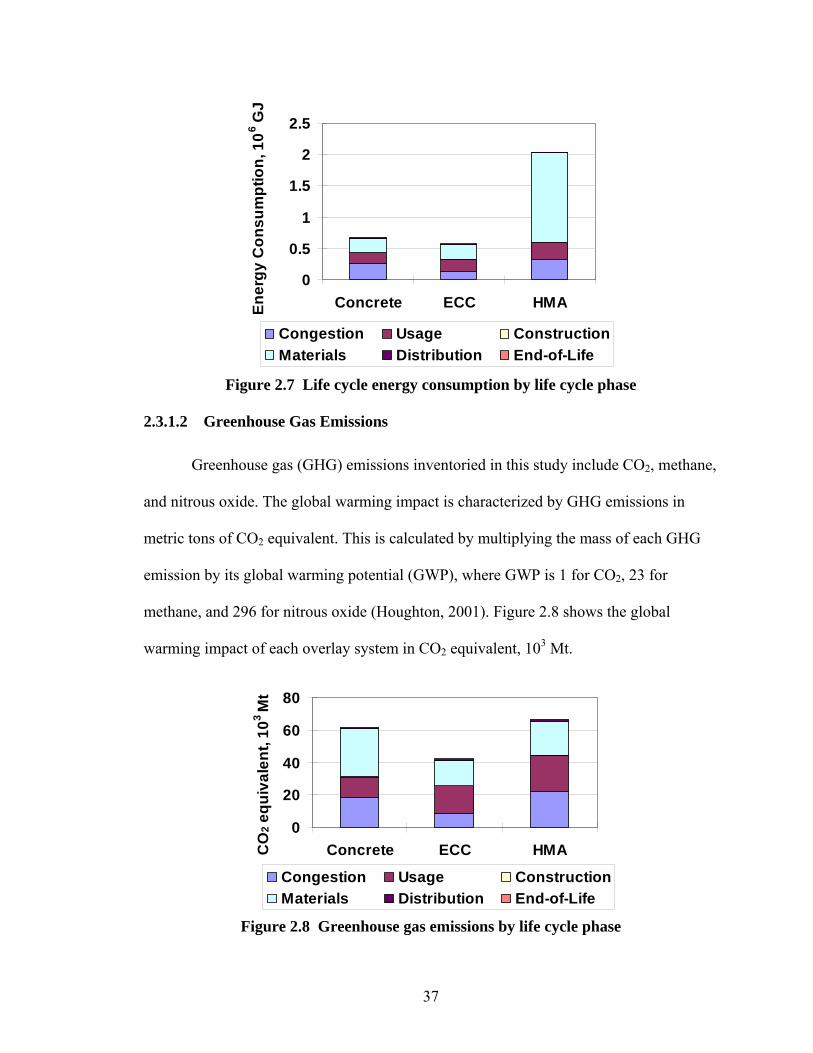
37
0
0.5
1
1.5
2
2.5
Concrete ECC HMAEner
gy C
onsu
mpt
ion,
106 G
J
Congestion Usage ConstructionMaterials Distribution End-of-Life
Figure 2.7 Life cycle energy consumption by life cycle phase
2.3.1.2 Greenhouse Gas Emissions
Greenhouse gas (GHG) emissions inventoried in this study include CO2, methane,
and nitrous oxide. The global warming impact is characterized by GHG emissions in
metric tons of CO2 equivalent. This is calculated by multiplying the mass of each GHG
emission by its global warming potential (GWP), where GWP is 1 for CO2, 23 for
methane, and 296 for nitrous oxide (Houghton, 2001). Figure 2.8 shows the global
warming impact of each overlay system in CO2 equivalent, 103 Mt.
0
20
40
60
80
Concrete ECC HMACO
2 equ
ival
ent,
103
Mt
Congestion Usage ConstructionMaterials Distribution End-of-Life
Figure 2.8 Greenhouse gas emissions by life cycle phase

38
CO2 emissions significantly dominate the contribution to global warming impact.
In the concrete overlay system CO2 represents 99.2% of total life cycle GWP, in the ECC
system CO2 represents 99.4% of total life cycle GWP, and in the HMA system CO2
represents 94.4% of total life cycle GWP. The ECC system reduces GHG emissions by
32% and 37% compared to the concrete overlay system and HMA overlay system,
respectively. Generally, CO2 emission reflects energy consumption; however, cement
production releases CO2 during calcination of limestone. Additionally, a large amount of
primary energy consumption in the HMA overlay system is the feedstock energy. Carbon
embodied in the material is fixed and does not generate CO2 unless it is burned. This
relationship is evident in the comparison of Figure 2.7 and Figure 2.8 wherein the CO2
emissions of the HMA overlay system are not significantly higher than the other two
systems.
2.3.1.3 Air Pollutant emissions
Other air pollutant emissions in addition to the GHG emissions in this analysis
include nitrogen oxides (NOx), sulfur oxides (SOx), nonmethane hydrocarbons (NMHC),
particulate matter (PM2.5), carbon monoxide (CO), and volatile organic compounds
(VOC). Figure 2.9 presents these air pollutant emissions by life cycle stage.

39
NOx
-100000
-50000
0
50000
100000
150000
Concrete ECC HMA
SOx
0
30000
60000
90000
120000
150000
Concrete ECC HMA
NMHC
0
10000
20000
30000
40000
Concrete ECC HMA
PM10
0
1000
2000
3000
4000
Concrete ECC HMA
Carbon Monoxide
-300000
-200000
-100000
0
100000
200000
Concrete ECC HMA
VOC
0
30000
60000
90000
120000
Concrete ECC HMA
NOx
-100000
-50000
0
50000
100000
150000
Concrete ECC HMA
SOx
0
30000
60000
90000
120000
150000
Concrete ECC HMA
NMHC
0
10000
20000
30000
40000
Concrete ECC HMA
PM10
0
1000
2000
3000
4000
Concrete ECC HMA
Carbon Monoxide
-300000
-200000
-100000
0
100000
200000
Concrete ECC HMA
VOC
0
30000
60000
90000
120000
Concrete ECC HMACongestion Usage Construction Materials Distribution End-of-LifeCongestion Usage Construction Materials Distribution End-of-Life
kg
Figure 2.9 Air emissions by life cycle phase
In most cases, material phase related emissions dominate total pollutant emissions.
The emissions of NOx and CO show negative values for the traffic congestion module
and usage module for all systems resulting from NOx and CO production being greater at
high speeds than at low speeds. While most pollutants increase with congestion and
overlay deterioration, NOx and CO emissions decrease (Sher, 1998). The large VOC
emissions associated with the HMA overlay system result from the evaporation of
petroleum distillate solvent, or diluent, used to liquify the asphalt cement during
maintenance. VOC emissions occur at both the construction site and the mixing plant.
The road surface emissions at the construction site are the largest source of emissions and
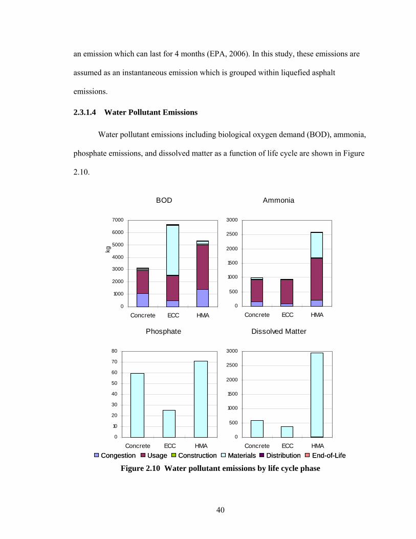
40
an emission which can last for 4 months (EPA, 2006). In this study, these emissions are
assumed as an instantaneous emission which is grouped within liquefied asphalt
emissions.
2.3.1.4 Water Pollutant Emissions
Water pollutant emissions including biological oxygen demand (BOD), ammonia,
phosphate emissions, and dissolved matter as a function of life cycle are shown in Figure
2.10.
BOD
0
1000
2000
3000
4000
5000
6000
7000
Concrete ECC HMA
Ammonia
0
500
1000
1500
2000
2500
3000
Concrete ECC HMA
Phosphate
0
10
20
30
40
50
60
70
80
Concrete ECC HMA
Dissolved Matter
0
500
1000
1500
2000
2500
3000
Concrete ECC HMA
BOD
0
1000
2000
3000
4000
5000
6000
7000
Concrete ECC HMA
Ammonia
0
500
1000
1500
2000
2500
3000
Concrete ECC HMA
Phosphate
0
10
20
30
40
50
60
70
80
Concrete ECC HMA
Dissolved Matter
0
500
1000
1500
2000
2500
3000
Concrete ECC HMACongestion Usage Construction Materials Distribution End-of-LifeCongestion Usage Construction Materials Distribution End-of-Life
kg
Figure 2.10 Water pollutant emissions by life cycle phase

41
For both BOD and ammonia emissions, the use phase has a significant effect on
total emissions. However, the PVA fiber used in ECC overlay system and asphalt used in
the HMA overlay system are also responsible for large BOD emissions and ammonia
emissions, respectively. For phosphate and dissolved matter emissions, the material phase
overwhelmingly dominates the total emissions.
Table 2.5 summarizes the life cycle impact results. The environmental impacts of
the ECC overlay system are listed in the table along with percentage changes relative to
concrete overlay and HMA overlay systems. As seen, ECC shows significant advantages
in many environmental impact categories.
Table 2.5 Summary of life cycle impact results
Item ECC vs. Concrete vs. HMA Total primary energy consumption, GJ 5.8×10⁵ -15% -72% GHG, mt 4.2×10⁴ -32% -37% Carbon Monoxide, kg 4.2×10⁴ +19% +30% VOC, kg 2.2×10⁴ -34% -81% NMHC, kg 2.2×10⁴ +137% -41% PM2.5, kg 1.3×10³ -11% -63% NOx, kg 7.3×10⁴ -26% +6% SOx, kg 7.3×10⁴ -42% -27% Ammonia, kg 1.0×10³ +5% -58% BOD, kg 7.0×10³ +102% +36% Dissolved matter, kg 3.8×10² -36% -87% Phosphates, kg 25.5 -57% -64% 2.3.2 Life Cycle Cost Analysis Results
Table 2.6 shows the results for life cycle costs. The ECC overlay system
demonstrates a cost advantage over the other two overlay systems in all cost categories
assessed.

42
Table 2.6 Life cycle costs for overlay systems
Concrete ECC HMA ECC cost advantage Agency cost $11.6m $7.4m $13.8m 36% User cost $67.5m $40.8m $77.6m 40% Environmental cost $0.9m $0.6m $1.1m 33% Total cost $80.0m $48.8m $92.5m 39%
User costs account for more than 80% of total life cycle costs in each overlay
system. Environmental costs are small compared to agency and user costs. Essentially,
the cost distribution is driven by traffic parameters. Since this research deals with a high
traffic volume freeway, congestion-related user time delays are significant. Thus, user
costs overwhelmingly dominate total life cycle costs. If assumed traffic volume is lower,
the likely impact of user costs on total life cycle costs will decrease and the impact of
agency costs and environmental costs will increase relative to the user costs.
A possible way to decrease the impact of construction and maintenance activities
is to apply night time construction and maintenance methods. Due to lower traffic volume
at night, the user time delay cost will be minimized. However, there is a potential
increase in labor cost and accidental cost.
Despite higher initial construction costs for the ECC overlay system, the lower
preservation frequency due to improved ECC material properties, it is estimated that
accumulated agency cost savings for ECC will result compared to the concrete and HMA
overlay systems. Figure 2.11 shows the cumulative life cycle costs for each overlay
system.

43
Figure 2.11 Cumulative life cycle costs for overlay systems 2.3.3 Sensitivity Analysis
The results discussed above assume a baseline scenario which has no traffic flow
growth or fuel economy improvements over time. Traffic flow growth will affect traffic
related energy consumption and costs by increasing total vehicle miles traveled and
congestion. Figure 2.12 shows the energy consumption and life cycle costs at different
traffic growth rate of 0%, 1%, and 2%, annually. In the baseline scenario, the ECC
overlay system uses 15% less total energy and 40% less life cycle costs than the concrete
overlay system. If traffic flow increases over time, the ECC overlay system will save
even more energy and costs than the concrete overlay system. The low traffic volume
scenarios are discussed in Appendix A.
0
20
40
60
80
100
2006 2011 2016 2021 2026 2031 2036 2041 2046
Year
Mill
ion
US
Dol
lars
(200
6)ConcreteECCHMA
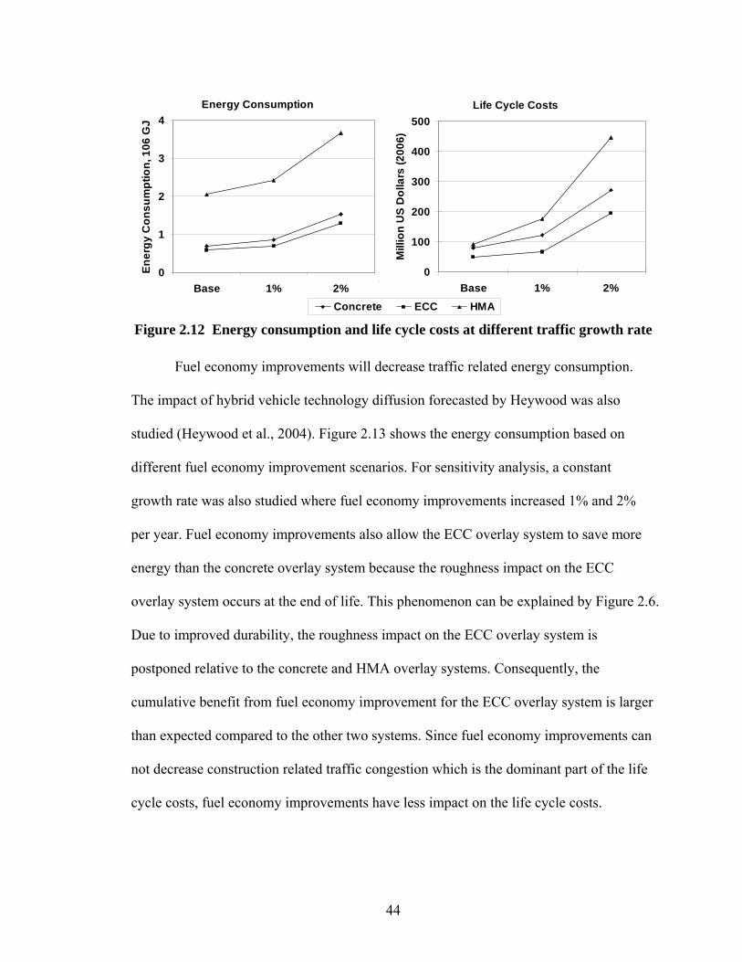
44
Concrete ECC HMA
Energy Consumption
0
1
2
3
4
Base 1% 2%
Ener
gy C
onsu
mpt
ion,
106
GJ
Life Cycle Costs
0
100
200
300
400
500
Base 1% 2%
Mill
ion
US
Dol
lars
(200
6)
Figure 2.12 Energy consumption and life cycle costs at different traffic growth rate
Fuel economy improvements will decrease traffic related energy consumption.
The impact of hybrid vehicle technology diffusion forecasted by Heywood was also
studied (Heywood et al., 2004). Figure 2.13 shows the energy consumption based on
different fuel economy improvement scenarios. For sensitivity analysis, a constant
growth rate was also studied where fuel economy improvements increased 1% and 2%
per year. Fuel economy improvements also allow the ECC overlay system to save more
energy than the concrete overlay system because the roughness impact on the ECC
overlay system occurs at the end of life. This phenomenon can be explained by Figure 2.6.
Due to improved durability, the roughness impact on the ECC overlay system is
postponed relative to the concrete and HMA overlay systems. Consequently, the
cumulative benefit from fuel economy improvement for the ECC overlay system is larger
than expected compared to the other two systems. Since fuel economy improvements can
not decrease construction related traffic congestion which is the dominant part of the life
cycle costs, fuel economy improvements have less impact on the life cycle costs.
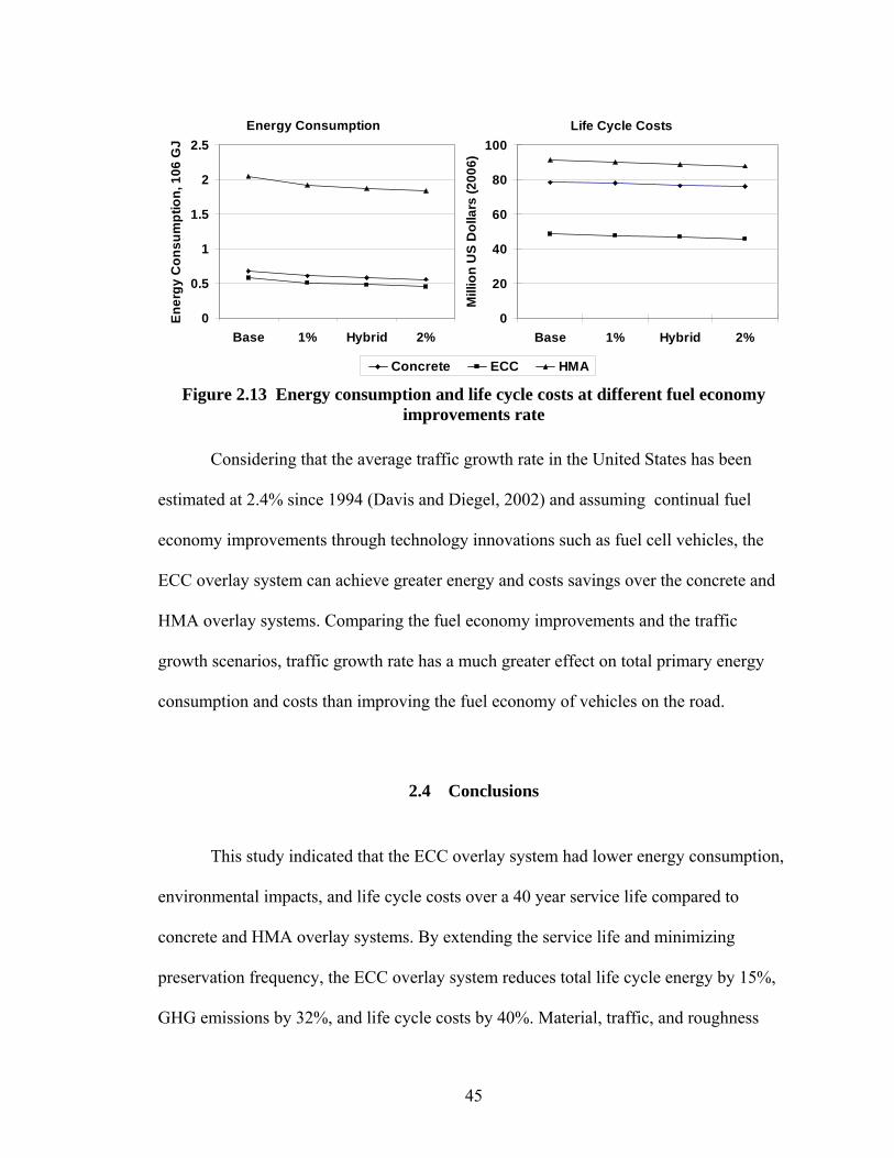
45
Concrete ECC HMA
Energy Consumption
0
0.5
1
1.5
2
2.5
Base 1% Hybrid 2%
Ener
gy C
onsu
mpt
ion,
106
GJ
Life Cycle Costs
0
20
40
60
80
100
Base 1% Hybrid 2%
Mill
ion
US
Dol
lars
(200
6)
Figure 2.13 Energy consumption and life cycle costs at different fuel economy
improvements rate
Considering that the average traffic growth rate in the United States has been
estimated at 2.4% since 1994 (Davis and Diegel, 2002) and assuming continual fuel
economy improvements through technology innovations such as fuel cell vehicles, the
ECC overlay system can achieve greater energy and costs savings over the concrete and
HMA overlay systems. Comparing the fuel economy improvements and the traffic
growth scenarios, traffic growth rate has a much greater effect on total primary energy
consumption and costs than improving the fuel economy of vehicles on the road.
2.4 Conclusions
This study indicated that the ECC overlay system had lower energy consumption,
environmental impacts, and life cycle costs over a 40 year service life compared to
concrete and HMA overlay systems. By extending the service life and minimizing
preservation frequency, the ECC overlay system reduces total life cycle energy by 15%,
GHG emissions by 32%, and life cycle costs by 40%. Material, traffic, and roughness

46
effects were identified as the greatest contributors to environmental impacts throughout
the overlay system life cycle. User costs significantly dominate total life cycle costs. The
analysis also showed the potential of environmentally preferable mixtures which use
industrial byproducts to substitute for energy intensive or environmentally harmful
materials, such as waste fly ash for Portland cement in the ECC overlay system (as noted
previously, this assumes no allocation of power plant environmental impacts to the waste
fly ash). This substitution results in significantly reduced raw material and energy
consumption, and decreased environmental burdens while maintaining or improving
overlay system performance.
Both the service life and preservation strategy are the key factors determining
overlay system performance. Alternative overlay design strategies, such as varying
overlay thickness and different maintenance schedules, can be implemented based on
local traffic loads and pavement requirements. Using this approach, the decision maker is
able to select an optimal overlay design for alternative materials.
The integrated LCA-LCCA model outlined in this chapter dynamically captures
cumulative traffic flows, overlay deterioration over time, and maintenance activities to
evaluate life cycle environmental burdens and costs. The incorporation of pavement
overlay roughness effects on fuel consumption and related life cycle environmental
burdens represents a significant extension of existing models. The resulting life cycle
model enables decision makers to evaluate pavement infrastructure projects from a more
holistic, long term perspective while providing criteria for more sustainable infrastructure
material selection.
47
References
American Society of Civil Engineering (ASCE). (2006). Road to Infrastructure Renewal—A Voter’s Guide. Reston, Va.
American Concrete Pavement Association (ACPA). (1990). Guidelines for Unbonded Concrete Overlays. ACPA, Skokie, Illinois.
Archonodo-Callao, R. S. (1999). Unpaved roads’ roughness estimation by subjective evaluation, Transport No. RT-2, The World Bank, Washington, D.C.
The Athena Sustainable Material Institute. (1999). Life cycle embodied energy and global warming emissions for concrete and asphalt roadways. The Athena Sustainable Material Institute, Canada.
Chan, A., Keoleian, G., and Gabler, E. (2006). “Evaluation of life-cycle cost analysis practices used by the Michigan Department of Transportation.” Journal of Transportation Engineering. Submitted.
Chandra, S. (2004). “Effect of road roughness on capacity of two-lane roads.” Journal of Transportation Engineering, 130 (3), 360-364.
Davis, S. C., and Diegel, S. W. (2002). Transportation energy data book, Center for Transportation Analysis. Oak Ridge National Laboratory, Tennessee.
Estakhri, C. K., and Saylak, D. (2005). “Reducing greenhouse gas emissions in Texas with high-volume fly ash concrete.” Transportation Research Record, 1941, 167-174.
Gilani, A. (2001). “Link slabs for simply supported bridges: Incorporating engineering cementitious composites.” MDOT SPR-54181, Structural Research Unit, Lansing, Michigan.
Heywood, J. B., Weiss, M. A., and Schafer, A. (2004). The performance of future ICE and fuel cell powered vehicle and their potential fleet impact. Laboratory for Energy and the Environment, Massachusetts Institute of Technology, Massachusetts.
48
Horvath, A., and Hendrickson, C. (1998). “Comparison of environmental implications of asphalt and steel-reinforced pavements.” Transportation Research Record, 1626, 105-113.
Huang, Y. H. (2004). Pavement analysis and design. University of Kentucky, Upper Saddle River, NJ.
The International Organization for Standardization (ISO). (1997). Environmental management: Lifecycle assessment: Principles and Framework. ISO 14040.
The International Organization for Standardization (ISO). (1998). Environmental management: Lifecycle assessment: Goal and scope definition and inventory analysis. ISO 14041.
The International Organization for Standardization (ISO). (2000). Environmental management: Lifecycle assessment: Life cycle impact assessment. ISO 14042.
Keoleian, G. A. and Kendall, A. (2005). “Life cycle modeling of concrete bridge design: Comparison of engineered cementitious composite link slabs and conventional steel expansion joints.” Journal of infrastructure systems, 11(1), 51-60.
Keoleian, G. A. and Spitzley, D.V. (2006). “Life Cycle Based Sustainability Metrics.” Chapter 7 in Sustainability Science and Engineering: Defining Principles (Sustainability Science and Engineering, Volume 1), M.A. Abraham, Ed. Elsevier, pp. 127-159.
Kendall, A., Keoleian, G. A., and Helfand, G. E. (2006). “Integrated life-cycle assessment and life-cycle analysis model for concrete bridge deck applications.” Journal of infrastructure systems, 14(3), 214-222.
Kentucky Transportation Center (KTC). (2002). The costs of construction delays and traffic control for life-cycle cost analysis of pavements. KTC-02-07/SPR197-99 &SPR218-00-1F, Lexington, Kentucky.
Langer, T. (2004). Energy saving through increased fuel economy for heavy-duty trucks. American Council for an Energy-Efficient Economy, Washington, D.C.

49
Lee, D., Chatti, K., and Baladi, G. Y. (2002). “Use of distress and ride quality data to determine roughness thresholds for smoothing pavements as a preventive maintenance action.” Transportation Research Record, 1816, Paper No. 02-4039
Li, V. C. (2003). “Durable overlay systems with engineered cementitious composites (ECC).” International Journal for Restoration of Buildings and Monuments, 9(2), 1-20.
Li, V. C. (2002). “Reflection on the research and development of engineered cementitious composites (ECC).” Proceeding of the JCI International Workshop on Ductile Fiber Reinforced cementitious composites (DRFCC-2002), Takayama, Japan, Oct. 2002, pp. 121-132
Li, V. C., and Fischer, G., “Reinforced ECC – an evolution from materials to structure.” Proceedings of the First FIB Congress, Osaka, Japan, Oct. 2002, pp. 105-122.
Lim, Y. M., and Li, V. C. (1997). “Durable repair of aged infrastructures using trapping mechanism of engineered cementitious composites.” Cement and Concrete Composites, 19, 373-385.
Michigan Department of Transportation (MDOT). (1997). 1997 Noninterstate freeway segments: Deficient segments-URBAN. MDOT, Ann Arbor, Michigan.
Michigan Department of Transportation (MDOT). (2002). Standard specifications for construction. MDOT, Ann Arbor, Michigan.
Michigan Department of Transportation (MDOT). (2005). Pavement desigan and selection manual. MDOT, Ann Arbor, Michigan.
Office of Management and Budget. (2005). Discount Rates for Cost-Effectiveness, Lease, Purchase and Related Analyses. Appendix C to Guidelines and Discount Rates for Benefit-Cost Analysis of Federal Programs. Office of Management and Budget: Washington D.C.
Portland Cement Association (PCA). (2002). Environmental life cycle inventory of Portland cement concrete. PCA, Skokie, Illinois.
Product Ecology Consultant (Pre). (2004). SimaPro 6.0. Pre, Netherlands.
50
Qian, S. (2007). “Influence of Concrete Material Ductility on the Behavior of High Stress Concentration Zones.” Doctoral thesis. University of Michigan, Ann Arbor, Michigan.
Sayers, M. W., Gillespie, T. D., and Queiroz, C. A. V. (1986). International Experiment to Establish Correlations and Standard Calibration Methods for Road Roughness Measurements. World Bank Technical Paper No. 45, Washington, D.C.
Sayers, M. W., and Karamihas, S. M. (1995). The Little Book of Profiling. University of Michigan Transportation Research Institute (UMTRI), Ann Arbor, Michigan.
Sher, E. (1998). Handbook of Air Pollution from Internal Combustion Engines. Academic Press, Boston.
Southeast Michigan Council of Governments (SEMCOG). (2006). Ozone and carbon monoxide conformity analysis for the proposed amendment of the 2030 regional transportation plan for Southeast Michigan. SEMCOG, Detroit, Michigan.
Spivey, J. (2000). VOC emissions from asphalt paving. Environmental Technology Verification (ETV) Stakeholder Advisory Committee meeting, Research Triangle Park, North Carolina.
Stripple, H. (2001). Life cycle assessment of road: A pilot study for inventory analysis. Swedish Environmental Research Institute (IVL), Gothenburg, Sweden.
Tunnell, M. A., and Brewster, R. M. (2005). “Energy and emissions impacts of operating higher-productivity vehicles.” Transportation Research Record, 1941, 107-114.
United States Department of Transportation (DOT). (1989). Rehabilitation of concrete pavements. Volume II, FHWA-RD-88-072, Washington, D.C.
United States Department of Energy (DOE). (2004). Vision model: Description of model used to estimate the impact of highway vehicle technologies and fuels on energy use and carbon emissions to 2050. Center for Transportation Research Argonne National Laboratory, DOE.
United States Environmental Protection Agency (EPA). (2001). “Asphalt paving.” Rep. No. EPA/454/R-97/004, EIIP Technical Report Series, Volume III, Chapter 17, Washington D.C.

51
United States Environmental Protection Agency (EPA). (2002). MOBILE 6.2. Ann Arbor, Michigan.
United States Environmental Protection Agency (EPA). (2005). NONROAD2005 model. USEPA, Ann Arbor, Michigan.
United States Environmental Protection Agency (EPA). (2006). Fuel economy labeling of motor vehicles: revisions to improve calculation of fuel economy estimates. Office of Transportation and Air Quality, Washington, D.C.
United States Environmental Protection Agency (EPA). (2006). “AP 42: Compilation of air pollutant emission factors.” Volume 1, Chapter 4, 5th edition, Washington, D.C.
Walls, J., III., and Smith, M. R. (1998). Pavement Division Interim Technical Bulletin:Life-Cycle Cost Analysis in Pavement Design - Interim Technical Bulletin. FHWA-SA-98-079, U.S. Department of Transportation, Federal Highway Administration, Washington D.C.
Weitzman, M. L. (2001). “Gamma discounting.” American Economic Review 91(1): 260-271.
WesTrack. (1999). The road to performance-related specifications. WesTrack Interim Reports, Nevada.
Wilson, A. (1993). “Cement and concrete: environmental considerations.” Environmental Building News, Vol. 2, No. 2, March/April.
Wilde, W. J., Waalkes, S., and Harrison, R. (2001). Life cycle cost analysis of Portland cement concrete pavement. University of Texas at Austin, Austin, Texas.
Zapata, P. and Gambatese, J. A. (2005). “Energy Consumption of Asphalt and Reinforced Concrete Pavement Material and Construction.” Journal of Infrastructure Systems, 11(1), 9-20.

52
CHAPTER 3
PROJECT-LEVEL PAVEMENT ASSET MANAGEMENT SYSTEM USING LIFE CYCLE OPTIMIZATION
ABSTRACT
Preservation strategy is the critical factor controlling pavement performance. A
project-level pavement asset management system (PAMS) was developed to determine
an optimal preservation strategy for a pavement overlay system. A life cycle optimization
(LCO) model was incorporated into the project-level pavement asset management system
to minimize life cycle energy consumption, GHG emissions, and costs within an analysis
period. Using dynamic programming optimization techniques, the LCO model integrates
dynamic life cycle assessment and life cycle cost analysis models with an autoregressive
pavement deterioration model. The project-level pavement asset management system was
applied to an ECC overlay system, a concrete overlay system, and a hot mixed asphalt
(HMA) overlay system. The results show that the optimal preservation strategies will
reduce the total life cycle energy consumption by 5%-30%, GHG emissions by 4%-40%,
and costs by 0.4%-12% for the concrete overlay system, the ECC overlay system, and the
HMA overlay system compared to the current Michigan Department of Transportation
preservation strategies, respectively. The impact of traffic growth on the optimal
preservation strategies is presented.
53
3.1 Introduction
Pavement structures and systems are fundamental elements of the automobile
transportation system in the United States. Shortfalls in budgets and increasing travel
demand have placed a significant burden on the transportation system. The
Transportation Equity Act for the 21st Century (TEA-21) provided $173 billion for
highway construction and maintenance over 6 years. However, even with TEA-21’s
commitment, another $27 billion is needed to improve conditions and performance of the
highway system, according the Federal Highway Administration (ASCE, 2006). The
budgetary pressure on highway agencies will result in the delay of many pavement
projects, and as a consequence decrease pavement performance. Thus, an effective
pavement asset management optimization approach, which allows highway agencies to
explore alternative pavement materials, predict pavement deterioration over time, assess
effectiveness of preservation strategies, and select optimal solution and design parameters,
becomes crucial. To address these needs, a project-level pavement asset management
system integrated with life cycle optimization, life cycle assessment, and life cycle cost
analysis methodologies has been applied to pavement overlay systems to more efficiently
allocate resources and improve pavement performance.
Pavement overlay preservation strategies identified in Chapter 2 are key factors in
the determination of overlay system energy consumption, environmental impacts, and
costs (Zhang et al., 2009). Since a pavement overlay can be preserved through a variety
of different maintenance and rehabilitation methods and frequencies, which leads to a set
of different life cycle energy consumption, environmental impacts, and costs, an analysis
resulting in a series of optimal solutions is necessary. Incorporating modern optimization

54
methods with LCA and LCCA concepts, pavement asset management system can
effectively improve pavement performance.
There are two major administrative levels of any pavement asset management
system: network-level PAMS and project-level PAMS (Mbwana, 2001). At the network-
level, the main objectives of PAMS are the establishment of a pavement segment
preservation priority selection scheme and a budget allocation strategy for the entire
pavement network. Working at a smaller scale, project-level PAMS determines the
optimal preservation strategy for a specified pavement segment by assessing pavement
deterioration, comparing and selecting alternative maintenance and rehabilitation
techniques and schedules, and evaluating design parameters such as pavement materials
and structures. Chapter 3 focuses on developing and analyzing a project-level PAMS
which provides detailed information for network-level PAMS.
Several project-level pavement asset management optimization methods have
been developed. Mamlouk developed a project-level optimization approach to minimize
the total costs of a flexible pavement (Mamlouk et al., 2000). This research demonstrated
the feasibility of combining modern optimization methods with empirical and
mechanistic prediction methods to identify cost-effective ways to manage pavement
systems. Mamlouk classified the total pavement costs as the agency costs and user costs.
While Mamlouk noted the increasing importance of social costs, the environmental
impacts and overlay roughness effects were not considered by his analysis.
Other models have also been developed for assisting pavement asset management,
such as the Highway Design and Maintenance model (HDM-4), developed by the World
Road Association (PIARC, 2002). This program predicts the consequences of different

55
maintenance and rehabilitation options and corresponding user benefits over time. The
major weakness is that it requires exogenously specified maintenance and rehabilitation
options for comparison. Accordingly, it is difficult to reach a global optimal result.
The objective of this chapter is to develop a project-level pavement asset
management system integrated with a life cycle optimization model to identify more
optimal pavement overlay preservation strategies based on the minimization of total life
cycle energy consumption, greenhouse gas emissions, or costs for pavement overlay
systems. Overlay deterioration, roughness effects, traffic congestion, traffic growth, and
preservation activities can be dynamically considered by this model. In addition, the LCO
model developed in this chapter enables decision makers to select an optimal overlay
preservation strategy more efficiently and accurately.
In this chapter, a pavement deterioration model and an LCO model will be
described and used to analyze the following three pavement overlay systems: concrete,
ECC, and HMA overlay systems. Subsequently, the optimal overlay maintenance and
rehabilitation strategies are identified to minimize the life cycle energy consumption,
environmental impacts, and economic costs of the concrete, ECC, and HMA overlay
systems.
3.2 Methodology
3.2.1 System Definition
The overlay designs analyzed in this study are the same designs presented in
Chapter 2. The overlays are constructed upon an existing reinforced concrete pavement

56
which was originally built by the Michigan Department of Transportation (MDOT). The
annual average daily traffic (AADT) is approximately 70,000 vehicles with 8% heavy
duty trucks (MDOT, 1997). In the baseline scenario, the annual traffic growth rate is 0%.
The three overlay systems are modeled as a 10 km long freeway in two directions. Based
on the results from experimental studies conducted at the University of Michigan and
typical pavement overlay designs (Qian, 2007; Huang, 2004), the concrete overlay and
HMA overlay are designed for a 20 year service life by MDOT (MDOT, 2005). The
service life of the ECC overlay is expected to be at least twice that of the concrete
overlay by preventing commonly observed overlay failure modes, such as reflective
cracking (Li, 2003).
3.2.2 Pavement Overlay Deterioration Model
In Michigan, a Distress Index (DI), representing a holistic measure of pavement
condition including both surface roughness and deterioration, is used rather than
International Roughness Index (IRI) to gauge pavement conditions (MDOT, 2005).
However, the DI and the IRI are correlated. No mechanics based theoretical model for
DI exists as it depends on many factors such as temperature, traffic flow and load, types
of pavements, and age of pavement. Many statistical models have been developed to
predict overlay deterioration, such as the S-shaped curve model, the Markov chain model,
and regression models (Ahmed et al., 2006). The selection of a particular model is based
on local conditions and deterioration rates of the pavement. Ahmed et al. found that an
auto-regression model produced the best prediction results for Michigan pavement DI
data (2006). Auto-regression uses the estimation of a stochastic process that can be
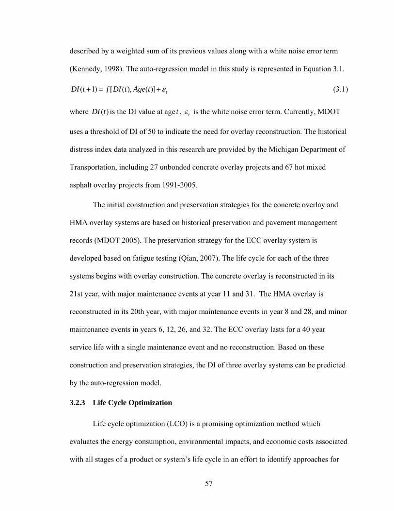
57
described by a weighted sum of its previous values along with a white noise error term
(Kennedy, 1998). The auto-regression model in this study is represented in Equation 3.1.
( 1) [ ( ), ( )] tDI t f DI t Age t ε+ = + (3.1)
where ( )DI t is the DI value at age t , tε is the white noise error term. Currently, MDOT
uses a threshold of DI of 50 to indicate the need for overlay reconstruction. The historical
distress index data analyzed in this research are provided by the Michigan Department of
Transportation, including 27 unbonded concrete overlay projects and 67 hot mixed
asphalt overlay projects from 1991-2005.
The initial construction and preservation strategies for the concrete overlay and
HMA overlay systems are based on historical preservation and pavement management
records (MDOT 2005). The preservation strategy for the ECC overlay system is
developed based on fatigue testing (Qian, 2007). The life cycle for each of the three
systems begins with overlay construction. The concrete overlay is reconstructed in its
21st year, with major maintenance events at year 11 and 31. The HMA overlay is
reconstructed in its 20th year, with major maintenance events in year 8 and 28, and minor
maintenance events in years 6, 12, 26, and 32. The ECC overlay lasts for a 40 year
service life with a single maintenance event and no reconstruction. Based on these
construction and preservation strategies, the DI of three overlay systems can be predicted
by the auto-regression model.
3.2.3 Life Cycle Optimization
Life cycle optimization (LCO) is a promising optimization method which
evaluates the energy consumption, environmental impacts, and economic costs associated
with all stages of a product or system’s life cycle in an effort to identify approaches for

58
minimizing these burdens. Current optimization techniques provide a scientific basis for
life cycle optimization. Based on different systems and problems, several optimization
techniques have been developed such as linear programming, integer programming, and
dynamic programming. Linear programming is a simple optimization technique and is
widely used in industry. However, most factors in this study, such as the overlay
deterioration, are not linear. This life cycle optimization is a discrete time multistage
decision making process. Dynamic programming is a nonlinear optimization technique
that is particularly applicable to problems requiring a sequence of interrelated decisions
(Dreyfus and Law, 1977). Each decision transforms the current situation into a new
situation. A sequence of decisions, which in turn yields a new sequence of situations, is
sought that minimizes (or maximizes) an objective function. The value of the objective
function for a sequence of decisions is generally equal to the sum of the value of the
individual decisions and situations in the sequence.
A recent LCO model developed for the optimization of generic vehicle
replacement provides a useful method for determining optimal lifetimes of products (Kim
et al., 2003). In this study, the dynamic programming technique was used to evaluate
optimal vehicle replacement strategies from energy, emissions, and cost perspectives.
Dynamic programming is computationally less intensive to solve multistage
decision making problems than enumeration methods which search for all possible results.
Dynamic programming takes advantage of avoiding full enumeration by eliminating early
partial decision solutions that cannot lead to the final optimal solution. It reduces a single
n-dimensional problem into n one-dimensional problems. Ideally, dynamic programming
seeks to translate one single complicated problem into several simple solvable problems.
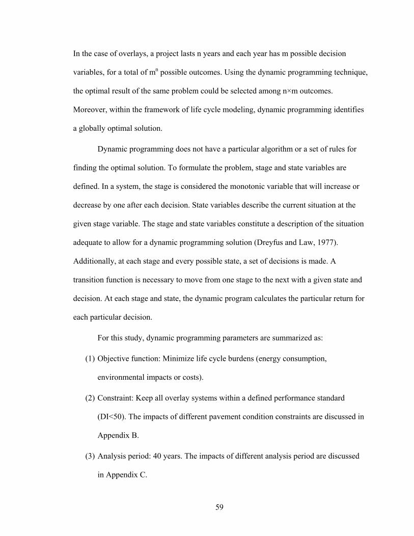
59
In the case of overlays, a project lasts n years and each year has m possible decision
variables, for a total of mn possible outcomes. Using the dynamic programming technique,
the optimal result of the same problem could be selected among n×m outcomes.
Moreover, within the framework of life cycle modeling, dynamic programming identifies
a globally optimal solution.
Dynamic programming does not have a particular algorithm or a set of rules for
finding the optimal solution. To formulate the problem, stage and state variables are
defined. In a system, the stage is considered the monotonic variable that will increase or
decrease by one after each decision. State variables describe the current situation at the
given stage variable. The stage and state variables constitute a description of the situation
adequate to allow for a dynamic programming solution (Dreyfus and Law, 1977).
Additionally, at each stage and every possible state, a set of decisions is made. A
transition function is necessary to move from one stage to the next with a given state and
decision. At each stage and state, the dynamic program calculates the particular return for
each particular decision.
For this study, dynamic programming parameters are summarized as:
(1) Objective function: Minimize life cycle burdens (energy consumption,
environmental impacts or costs).
(2) Constraint: Keep all overlay systems within a defined performance standard
(DI<50). The impacts of different pavement condition constraints are discussed in
Appendix B.
(3) Analysis period: 40 years. The impacts of different analysis period are discussed
in Appendix C.

60
(4) State: DI values.
(5) Stage: Each year in the analysis period.
(6) Decision variables: No maintenance, minor maintenance, and major maintenance.
(7) Transition function: Auto-regression DI prediction model.
(8) Return: Expected cumulative burdens at each stage and state.
3.2.4 Life Cycle Optimization Model Operation
The life cycle optimization process uses a backward dynamic programming
procedure starting the computation at year N, the final year of the analysis period. The
mathematical model for dynamic programming is constructed by first calculating the
current overlay system burdens, as described by Equation 3.2.
( , ) ( , ) ( , ) ( , ) ( , ) ( , ( )) 0( , )
0 0M C D CG E UB i j B i j B i j B i j B i j B i DI i if i
U i jif i
+ + + + + >⎧= ⎨ =⎩
(3.2)
where i is the current stage, j is the maintenance alternative, ( , )MB i j is the burden
associated with the material module at year i with decision j . Similarly, ( , )CB i j ,
( , )DB i j , ( , )CGB i j , and ( , )EB i j are the burdens of construction, distribution, traffic
congestion, and end of life modules, respectively, at year i with decision j . ( , ( ))UB i DI i
is the burden of overlay usage which is caused by overlay roughness effects at year i
with a particular distress index.
Equation 3.3 is used to calculate the total burdens from year N to year n.
{ }0,1,2
min ( , ) ( 1) ,...,( )
0j
U i j f i i n Nf i
i N=
⎧ + + ∀ =⎪= ⎨∀ >⎪⎩
(3.3)

61
where ( )f i is the minimum possible burden accumulated from year n to the end of year
N given a particular maintenance alternative.
A computer program using Visual Basic (VBA) and running within Microsoft
Excel software was coded to implement the LCO model and link it to the integrated
LCA-LCCA model. A flowchart of the LCO model operation is shown in Figure 3.1.
Figure 3.1 LCO model operation flowchart using dynamic programming

62
3.3 Results and Discussions
3.3.1 Life Cycle Optimization Results
The LCO model is used to determine optimal preservation strategies based on the
integrated LCA-LCCA results. Optimizations are conducted to minimize life cycle
energy consumption, GHG emissions, and total costs. The results also show the impacts
of optimal preservation strategy on criteria pollutant emissions. The optimal preservation
strategies and the original preservation strategies (MDOT strategies for the concrete and
HMA overlay systems, experimental planning for the ECC overlay system) for the three
overlay systems are shown in Figure 3.2. The optimal preservation strategy to minimize
energy consumption and GHG emissions for the concrete overlay system involves
constructing an initial overlay in year 2006 (the first year), performing four major
maintenance activities in year 2015, 2019, 2036, 2040, and reconstructing in year 2027.
The optimal preservation strategies to minimize energy consumption and GHG emissions
are identical and driven by reductions in fossil fuel combustion, which contribute
predominately to both energy consumption and GHG emissions for each overlay system.
Figure 3.2 presents the maintenance and rehabilitation schedule for energy/GHG
objectives. It demonstrates more frequent preservation activities than the maintenance
and rehabilitation schedule for cost minimization objectives. This phenomenon can be
attributed to the dominance of user time delay costs as a part of user costs. User time
delay costs are related to the traffic congestion caused by preservation activities.
Therefore, minimizing maintenance and rehabilitation frequency or substituting several
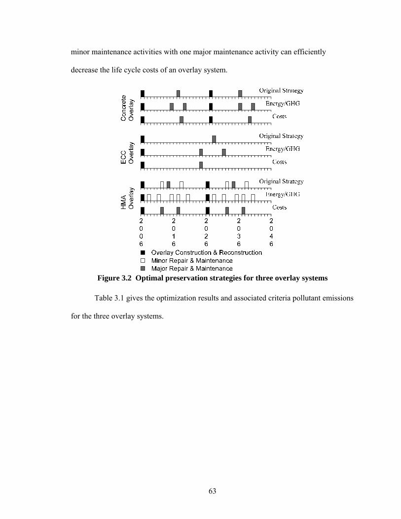
63
minor maintenance activities with one major maintenance activity can efficiently
decrease the life cycle costs of an overlay system.
Figure 3.2 Optimal preservation strategies for three overlay systems
Table 3.1 gives the optimization results and associated criteria pollutant emissions
for the three overlay systems.

64
Table 3.1 Life cycle burdens of optimal preservation strategies for each overlay
system
Life cycle burdens Optimization objectives
Energy
(105 GJ)
GHG
(104mt CO2 equiv)
SOx
(105 kg)
NOx
(105 kg)
PM2.5
(102 kg)
Energy/GHG 6.40 5.96 1.33 1.02 16.3 Concrete
Costs 7.30 6.58 1.29 1.02 24.4
Energy/GHG 4.44 3.14 0.70 0.72 6.81 ECC
Costs 5.20 3.76 0.71 0.70 12.8
Energy/GHG 14.3 3.98 0.74 0.53 23.0 HMA
Costs 22.3 5.69 1.08 0.61 25.6
Life cycle burdens
Pb
(kg)
VOC
(104 kg)
CO
(104 kg)
Cost
(107 $)
Energy/GHG 6.19 3.83 -7.36 8.99 Concrete
Costs 5.67 3.44 1.0 7.80
Energy/GHG 2.33 2.33 -1.06 5.36 ECC
Costs 2.13 2.19 2.85 4.85
Energy/GHG 3.41 4.41 -5.63 10.3 HMA
Costs 5.17 1.88 1.63 8.43
(note: values shown in table should not imply three significant figures; they are provided to avoid potential rounding errors)
65
The negative value of CO emissions results from greater CO tailpipe emissions at
high speeds as compared to low speeds. Therefore, congestion delays effectively decrease
CO emissions (Sher, 1998; US EPA, 2002). Compared to the original preservation
strategies (MDOT strategies for the concrete and HMA overlay systems, experimental
planning for the ECC overlay system), energy/GHG optimal strategies save 6%, 23%,
and 30% of life cycle energy consumption, and 4%, 25%, and 40% of GHG emissions for
the concrete overlay system, ECC overlay system, and HMA overlay system, respectively.
Since LCCA has been required by MDOT in the design of all projects with paving costs
greater than $1 million since 1998, cost optimal strategies save 0.4%, 0.5%, and 8% of
costs for concrete overlay system, ECC overlay system, and HMA overlay system,
respectively.
As shown in Figure 3.3, the trade-offs between material consumption, traffic
congestion, and roughness effects (captured in the usage phase) play an important role in
identification of optimal preservation strategies. For energy/GHG objectives, reducing
roughness effects that impact vehicle fuel economy is an effective way to decrease the
overall energy consumption and GHG emissions, even though energy consumption and
GHG emissions increase during maintenance and rehabilitation events due to traffic
congestion. For cost objectives, the optimal strategy is opposite to that of energy/GHG
objectives. User time delay costs caused by traffic congestion dominate total life cycle
costs. An effective way to decrease the total life cycle cost is to decrease the maintenance
and rehabilitation frequency and thereby user time delay costs. Moving from a cost
objective to energy/GHG objectives increases economic costs from 11% to 22%.

66
However, the relative magnitude of the decrease in energy consumption ranges from 12%
to 36% and the decrease in GHG emission ranges from 10% to 30%.
Energy Consumption of the HMA OverlaySystem
0.0
5.0
10.0
15.0
20.0
25.0
Original Design Energy/GHGOptimization
105
GJ
Congestion Usage ConstructionMaterials Distribution End-of-Life
GHG Emissions of the HMA Overlay System
0.0
2.0
4.0
6.0
8.0
Origina l De sign Ene rgy/GHGOptim iza tion
104
Mt
CO
2eq
uiva
len
t
Cong e stion Usa ge Con struction
M a te ria ls Distribu tion End -of-Life
Costs of the HMA Overlay System
0.0
2.0
4.0
6.0
8.0
10.0
Origina l De sign Cost Optim iza tion
107
Do
llar
s
Age ncy costs Cong e stion costs
Usa ge costs Environ m e nta l costsEnergy Consumption of the ECC Overlay
System
0.0
2.0
4.0
6.0
Origina l De sign Ene rgy/GHGOptim iza tion
105
GJ
Cong e stion Usa ge Con struction
M a te ria ls Distribu tion End -of-Life
GHG Emissions of the ECC Overlay System
0.0
1.0
2.0
3.0
4.0
5.0
Origina l De sign Ene rgy/GHGOptim iza tion
104
Mt
CO
2eq
uiva
len
t
Cong e stion Usa ge Con struction
M a te ria ls Distribu tion End -of-Life
Costs of the ECC Overlay System
0.0
1.0
2.0
3.0
4.0
5.0
Origina l De sign Cost Optim iza tion
107
Do
llar
s
Age ncy costs Cong e stion costs
Usa ge costs Environ m e nta l costsEnergy Consumption of the Concrete
Overlay System
0.0
2.0
4.0
6.0
8.0
Origina l De sign Ene rgy/GHGOptim iza tion
105
GJ
Cong e stion Usa ge Con struction
M a te ria ls Distribu tion End -of-Life
GHG Emissions of the Concrete OverlaySystem
0.0
2.0
4.0
6.0
8.0
Origina l De sign Ene rgy/GHGOptim iza tion
104
Mt
CO
2eq
uiva
len
t
Cong e stion Usa ge Con struction
M a te ria ls Distribu tion End -of-Life
Costs of the Concrete Overlay System
0.0
2.0
4.0
6.0
8.0
Origina l De sign Cost Optim iza tion
107
Do
llar
s
Age ncy costs Cong e stion costs
Usa ge costs Environ m e nta l costs Figure 3.3 Comparison of energy consumption, GHG emissions and costs for
MDOT preservation strategies and optimal strategies for a. HMA, b. ECC, and c. Concrete overlay systems
3.3.2 Traffic Growth Scenario
The optimal preservation strategies discussed above are designed with no
assumed traffic flow growth over time. However, traffic growth will affect user costs,
traffic related energy consumption, and pollutant emissions by increasing total vehicle
miles traveled and overall system congestion. These factors will change the optimal
preservation strategy for each overlay system. Figure 3.4 shows the optimal preservation
strategies with a 2% annual traffic growth rate. The maintenance and rehabilitation
frequency decreases and preservation activities occur earlier avoiding higher costs from
future high traffic volumes.

67
Figure 3.4 Optimal preservation strategies for three overlay systems with 2%
annual traffic growth rate
Figure 3.5 shows the total life cycle results with annual traffic growth rates
increasing from 0 to 2%. As can be seen, with 2% annual traffic growth, the original
preservation strategies (MDOT strategies for the concrete and HMA overlay systems,
experimental planning for the ECC overlay system) which neglect traffic growth are
inefficient. Energy consumption, GHG emissions, and costs increase dramatically with
increased traffic flow. Compared to the original preservation strategies (MDOT strategies
for the concrete and HMA overlay systems, experimental planning for the ECC overlay
system), energy/GHG optimal strategies save 4%, 18%, and 14% of energy consumption,
and 4%, 18%, and 8% of GHG emissions for the concrete overlay system, ECC overlay
system, and HMA overlay system, respectively. Cost optimized preservation planning

68
saves 3%, 36%, and 14% of total life cycle costs for the concrete overlay system, ECC
overlay system, and HMA overlay system, respectively.
0.010.020.030.040.050.0
Bas
eli
ne
107
Dol
lars
Original design-Concrete Costs design-ConcreteOriginal design-ECC Costs design-ECC
Original design-HMA Costs design-HMA
GHG Emissions
0.0
5.0
10.0
15.0
20.0
Baseline scenario 2% traffic growth
104
MtC
O2
equi
vale
nt
Original design-Concrete Energy/GHG design-ConcreteOriginal design-ECC Energy/GHG design-ECCOriginal design-HMA Energy/GHG design-HMA
Costs
0.0
10.0
20.0
30.0
40.0
50.0
Baseline scenario 2% traffic growth
107
Dol
lars
GHG Emissions
0.0
5.0
10.0
15.0
20.0
Baseline scenario 2% traffic growth
104
MtC
O2
equi
vale
nt
EnergyConsumption
0.0
10.0
20.0
30.0
40.0
Baseline scenario 2% traffic growth
105
GJ
0.0
10.0
20.0
30.0
40.0
50.0
Baseline scenario 2% traffic growth
107
Dol
lars
0.0
5.0
10.0
15.0
20.0
Baseline scenario 2% traffic growth
104
MtC
O2
equi
vale
nt
0.0
10.0
20.0
30.0
40.0
Baseline scenario 2% traffic growth
105
GJ
Energy Consumption GHG Emissions Costs
Figure 3.5 Life cycle results with different annual traffic growth rate
3.4 Conclusion
This chapter describes the development of a new life cycle optimization model
and its application to a project-level pavement asset management system. Three potential
overlay systems were evaluated: a concrete overlay system, an ECC overlay system, and
an HMA overlay system. Construction events, traffic congestion, and roughness effects
are dynamically captured by the LCO model. Model results show that the optimal
preservation strategies will reduce by 5%-30% the total life cycle energy consumption,
4%-40% the GHG emissions, and 0.4%-12% the cost for concrete overlay system, ECC
overlay system, and HMA overlay system, respectively, when no traffic growth is
considered. Since MDOT has incorporated LCCA into pavement design already, total life
cycle costs have been controlled nearly to the optimal results.
However, MDOT’s pavement designs cannot dynamically capture traffic flow
changes. Results show that the preservation strategy is highly sensitive to traffic flow.
With a 2% annual traffic growth rate, the optimal preservation strategies show more
69
advantage when compared to original preservation strategies (MDOT strategies for the
concrete and HMA overlay systems, experimental planning for the ECC overlay system).
Due to improved material properties and extended service life, under any traffic
growth scenario, the ECC overlay system shows superior advantages in energy
consumption, GHG emissions, and cost, compared to the concrete overlay system and
HMA overlay system.
The application of dynamic programming as an optimization tool in life cycle
optimization of pavement overlay systems has great potential for obtaining outputs
considerably faster and more accurately compared to conventional methods. The
combination of modern optimization techniques and life cycle analysis methods improves
the management capability of transportation agencies as compared to current pavement
management practice.
This study highlights the trade-offs between material consumption, traffic
congestion, and pavement surface roughness effects. Energy/GHG optimization leads to a
more frequent preservation strategy, while cost optimization favors a less frequent
preservation strategy. These results also demonstrate the importance of including user
costs and roughness effects in pavement management and accounting. The methodology
developed during this study should lead to more cost effective and environmentally
sensitive pavement asset management system.
70
References
Ahmed, K., Abu-Lebdeh, G., and Lyles, R. W. (2006). “Prediction of pavement distress index with limited data on causal factors: an auto-regression approach.” The International Journal of Pavement Engineering, 7(1), 23-35.
American Society of Civil Engineering (ASCE). (2006). Road to Infrastructure Renewal—A Voter’s Guide, Reston, Va.
Chan, A., Keoleian, G., and Gabler, E. (2006). “Evaluation of life-cycle cost analysis practices used by the Michigan Department of Transportation.” Journal of Transportation Engineering. Submitted.
Dreyfus, S. F., and Law, A. M. (1977). The Art and Theory of Dynamic Programming. Academic Press, New York, NY.
Huang, Y. H. (2004). Pavement analysis and design, University of Kentucky, Upper saddle River, NJ.
Li, V. C. (2003). “Durable overlay systems with engineered cementitious composites (ECC).” International Journal for Restoration of Buildings and Monuments, 9(2), 1-20.
Kennedy, P. (1998). A guide to econometrics, MIT Press, Cambridge, MA.
Kendall, A., Keoleian, G. A., and Helfand, G. E. (2006). “Integrated life-cycle assessment and life-cycle cost analysis model for concrete bridge deck applications.” Journal of Infrastructure Systems, 14(3), 214-222.
Keoleian, G. A., Kendall, A., and Dettling, J. E. et al (2005). “Life cycle modeling of concrete bridge design: Comparison of engineered cementitious composite link slabs and conventional steel expansion joints.” Journal of infrastructure systems, 11(1), 51-60.
Keoleian, G. A. and Spitzley, D.V. (2006). “Life Cycle Based Sustainability Metrics.” Chapter 7 in Sustainability Science and Engineering: Defining Principles (Sustainability Science and Engineering, Volume 1), M.A. Abraham, Ed. Elsevier, pp. 127-159.
71
Kim, H. C., Keoleian, G. A., Grande, D. E., and Bean, J. C. (2003). “Life cycle optimization of automobile replacement: Model and application.” Environmental Science and Technology, Vol. 37, 5407-5413.
Mamlouk, M. S., Zaniewski, J. P., and He, W. (2000). “Analysis and design optimization of flexible pavement.” Journal of Transportation Engineering, 126 (2), 161-167.
Mbwana, J. R. (2001) A framework for developing stochastic multi-objective pavement management system. Technology Transfer in Road Transportation in Africa, Arusha, Tanzania.
Michigan Department of Transportation (MDOT). (1997). 1997 Noninterstate freeway segments: Deficient segments-URBAN, MDOT, Ann Arbor, Michigan.
Michigan Department of Transportation. (2002). “Michigan Transportation Facts & Figures 2001. Highways.” Lansing, MI.
Michigan Department of Transportation (MDOT). (2005). Pavement desigan and selection manual, MDOT, Ann Arbor, Michigan.
PIARC, Highway Development and Management Model, HDM-4. International study of highway development and management, World Road Association, PIARC, Paris, France.
Product Ecology Consultant (Pre). (2007). SimaPro 7.0, PRe, Netherlands.
Qian, S. (2007). “Influence of Concrete Material Ductility on the Behavior of High Stress Concentration Zones.” Doctoral thesis. University of Michigan, Ann Arbor, Michigan.
Sher, E. (1998). Handbook of air pollution from internal combustion engines, Academic Press, Boston.
Zhang, H., Lepech, M. D., Keoleian, G. A., Qian, S. Z., and Li, V. C. (2009) “Dynamic life cycle modeling of pavement overlay systems: capturing the impacts of users, construction, and roadway deterioration.” To be submitted to Journal of Infrastructure Systems.

72
CHAPTER 4
MULTI-OBJECTIVE AND MULTI-CONSTRAINT OPTIMIZATION IN PROJECT-LEVEL PAVEMENT ASSET MANAGEMENT: INFORMING
POLICY AND ENHANCING SUSTAINABILITY
ABSTRACT
Pavement preservation (maintenance and rehabilitation) requires large resource
investments and generates significant environmental impacts. Multi-constraint and multi-
objective optimization was conducted to study the impact of agency budget constraints on
user costs and total life cycle cost, identify the trade-offs between energy consumption
and costs, and understand the relationships among material consumption, traffic
congestion, and pavement roughness effects. A case study of a hot mixed asphalt (HMA)
overlay system shows that a reduction in total agency preservation budget from $2
million to $0.5 million increases the total life cycle cost from $54 million to $61 million
over a 20 year service life. A Pareto optimal solution that minimizes energy and cost
objectives was also developed to enhance the preservation strategies. The influence of
fuel taxes and government subsidies on a PAMS is explored and specific policy
recommendations are provided. For example, proposals by presidential candidates
Clinton and McCain to temporarily suspend the gas tax in the summer of 2008 would
have had a detrimental life cycle societal cost impact.

73
4.1 Introduction
The national highway system is an important public investment designed to
support the national economy by transporting goods and people. The American Society
of Civil Engineers (ASCE) estimates that $54 billion is invested in pavement preservation
each year (ASCE, 2005). However, the Federal Highway Administration estimates that
an additional $27 billion in pavement preservation is needed to ensure adequate
improvement in highway condition and performance (ASCE, 2006). The budgetary
pressure delays many pavement projects and decreases the pavement serviceable level
(OECD, 1994). Thus, an effective pavement asset management system (PAMS) is needed
to facilitate highway agencies to allocate their limited budgets cost efficiently.
Researchers and practitioners have developed applied mathematical models to
pavement asset management. In 1982, the state of Arizona developed a pavement
management system to optimize maintenance policies for its highway network (Golabi et
al., 1982). This system was based on linear programming and focused on minimizing cost.
Later, the Organization for Economic Cooperation and Development (OECD) examined
the use of life cycle cost principles for allocating resources to road maintenance (OECD,
1994). Fwa et al. applied genetic algorithms for solving multi-objective pavement
maintenance problems (Fwa et al., 2000). In their research, the concept of Pareto
efficiency was adopted to perform two and three objective optimization. Currently, the
Michigan Department of Transportation (MDOT) relies on the Michigan Road Quality
Forecasting System (RQFS) to develop preservation strategies for regional DOT
management districts. This RQFS software package uses current pavement condition data
from the pavement management system to predict future network conditions at different
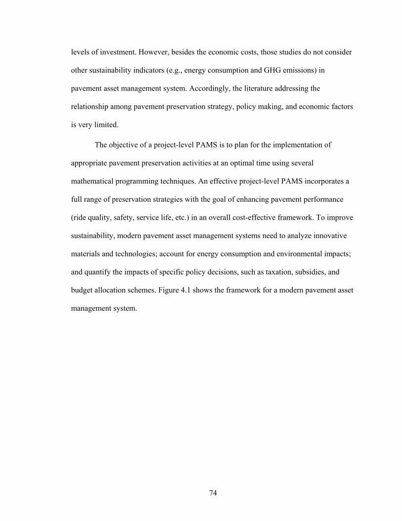
74
levels of investment. However, besides the economic costs, those studies do not consider
other sustainability indicators (e.g., energy consumption and GHG emissions) in
pavement asset management system. Accordingly, the literature addressing the
relationship among pavement preservation strategy, policy making, and economic factors
is very limited.
The objective of a project-level PAMS is to plan for the implementation of
appropriate pavement preservation activities at an optimal time using several
mathematical programming techniques. An effective project-level PAMS incorporates a
full range of preservation strategies with the goal of enhancing pavement performance
(ride quality, safety, service life, etc.) in an overall cost-effective framework. To improve
sustainability, modern pavement asset management systems need to analyze innovative
materials and technologies; account for energy consumption and environmental impacts;
and quantify the impacts of specific policy decisions, such as taxation, subsidies, and
budget allocation schemes. Figure 4.1 shows the framework for a modern pavement asset
management system.
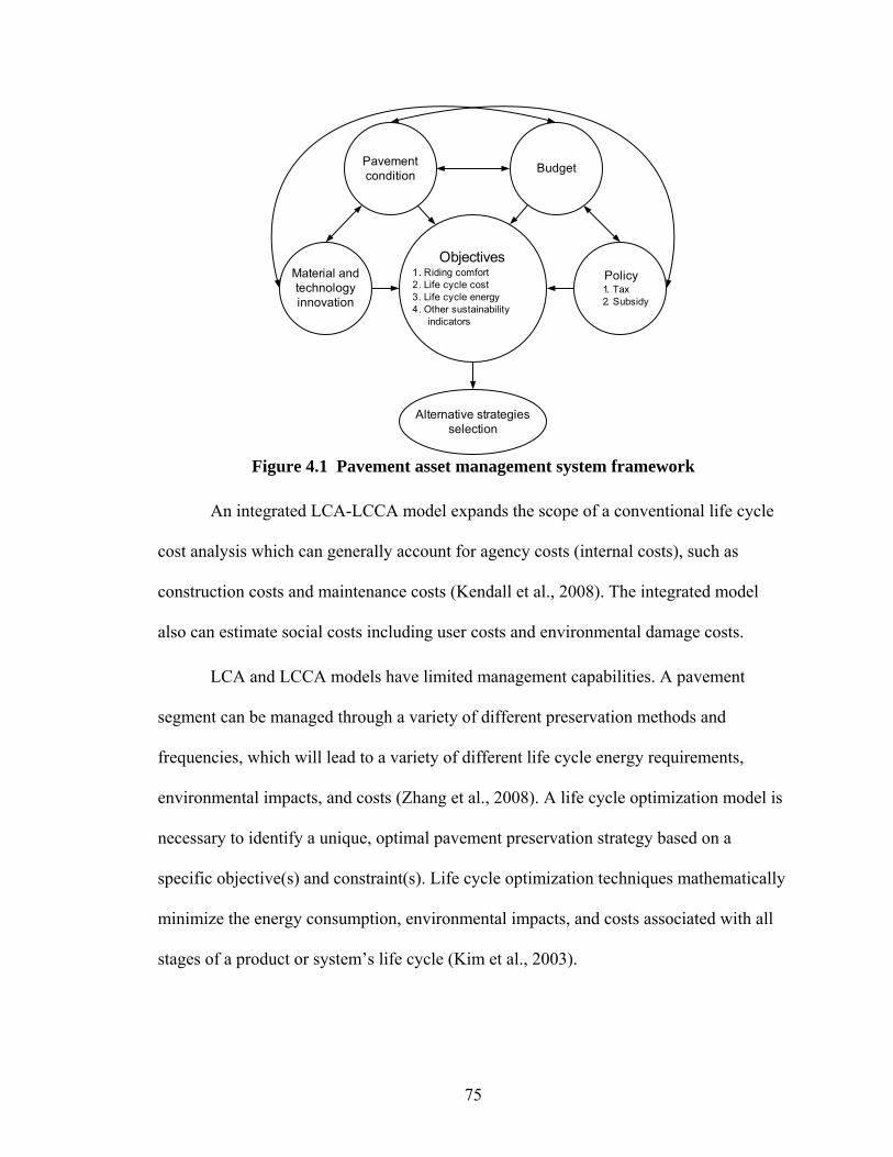
75
Objectives1. Riding comfort2. Life cycle cost3. Life cycle energy4. Other sustainability indicators
Material and technology innovation
Pavement condition Budget
Policy 1. Tax 2. Subsidy
Alternative strategies selection
Figure 4.1 Pavement asset management system framework
An integrated LCA-LCCA model expands the scope of a conventional life cycle
cost analysis which can generally account for agency costs (internal costs), such as
construction costs and maintenance costs (Kendall et al., 2008). The integrated model
also can estimate social costs including user costs and environmental damage costs.
LCA and LCCA models have limited management capabilities. A pavement
segment can be managed through a variety of different preservation methods and
frequencies, which will lead to a variety of different life cycle energy requirements,
environmental impacts, and costs (Zhang et al., 2008). A life cycle optimization model is
necessary to identify a unique, optimal pavement preservation strategy based on a
specific objective(s) and constraint(s). Life cycle optimization techniques mathematically
minimize the energy consumption, environmental impacts, and costs associated with all
stages of a product or system’s life cycle (Kim et al., 2003).
76
The objective of this chapter is to develop a project-level pavement asset
management system which incorporates integrated LCA-LCCA and LCO models. Multi-
objective and multi-constraint optimization is applied to balance the complex interactions
among material consumption, traffic congestion, and pavement roughness effects. The
application of this research to policy making is also explored. The impacts of fuel taxes,
government subsidies, and fuel prices on pavement preservation strategies and the
resulting energy consumption and life cycle costs are calculated.
4.2 Methodology
4.2.1 Expanded Project-Level Pavement Asset Management System
To improve the flexibility of a decision making process, the project-level
pavement asset management system developed in the Chapter 3 is expanded to
incorporate budget constraints and objective selection consideration. Figure 4.2 shows the
process flowchart of the expanded project-level pavement asset management system.
Previous developed project-level pavement asset management system using LCA model,
LCCA model, and LCO model evaluates the sustainability indicators and optimizes the
preservation strategy based on single constraint (pavement condition) and single
objective (energy consumption, environmental impacts, or costs). This single criteria
optimization gives highway agencies a limited ability to allocate economic resources
under budgetary constraints and develop a global optimal preservation strategy to achieve
maximum benefit. To solve this problem and further enhance sustainability, multi-

77
constraint optimization and multi-objective optimization models are developed in the
following sections.
LCA Model LCCA Model
LCO Model
Maintenance Strategy
Budget Constraint
Objective Functions
Material Development and
Selection
Figure 4.2 The process of project-level pavement asset management system
4.2.2 Multi-Constraint Optimization Model
Generally, highway agencies face at least two constraints: a minimum level of
allowable pavement condition (i.e. roughness) and a budgetary ceiling that cannot be
exceeded. For illustration, in Michigan the pavement condition is measured by a distress
index (DI). The DI value starts at 0 which indicates perfect pavement condition.
Although there is no upper limit for the DI value, the Michigan Department of
Transportation (MDOT) uses a threshold DI of 50 to indicate the need for pavement
rehabilitation or reconstruction (Ahmed et al., 2006). The budget represents the total
available resources for a highway agency to allocate among various maintenance and
rehabilitation activities for a set of pavement assets in any given year.
Figure 4.3 shows the hypothetical relationship between pavement condition and
costs. At lower budget levels, highway agencies have limited resources to perform

78
necessary maintenance and rehabilitation activities. This existing poor pavement
condition causes higher user costs and environmental costs through reduced fuel
efficiency. With a relaxed budget constraint, necessary maintenance and rehabilitation
activities can be implemented. Agency costs increase, however, pavement conditions are
improved. As a result, both user costs and environmental costs decrease because a
smoother pavement surface is provided to the users. However, if too many maintenance
and rehabilitation activities are performed or highway agencies apply inappropriate
maintenance and rehabilitation methods at sub-optimal times which interrupt normal
traffic flow and cause traffic congestion, generally, user costs, environmental costs, and
as a consequent, total life cycle cost increase. Together, pavement condition and available
budget determine the total life cycle cost for a pavement system. The objective of multi-
constraint optimization is to determine the minimum total life cycle cost at point O and
the associated preservation strategy to reach this point.
Pavement condition
Cos
tLo
wH
igh
Poor Good
Total life cycle cost
User cost
Environmental cost
Agency cost
O
Figure 4.3 A hypothetical relationship between pavement condition and cost
The objective function of the multi-constraint optimization is:
0
min ( , )N
t t tt
C R q m=
⎡ ⎤= ⎢ ⎥⎣ ⎦∑ (4.1)
79
Subject to
( )
00
50
N
tt
t
q S
m Max DI=
=
<
∑ (4.2)
where C is the total life cycle cost (or other objective, such as energy consumption). tR
is the total life cycle cost at year t . tq is the agency cost at year t . 0S is the budget
constraint, tm is the DI value at year t , and 0m equals to 0 (new pavement condition).
In order to solve the problem, a Lagrange multiplier is used to reduce the
dimension of formulation (Dreyfus and Law, 1977). The following four steps are
employed:
(1) Choose a positive value of the Lagrange multiplier λ . λ is also called the
shadow price at the optimal solution. The shadow price represents the change in
objective function due to an infinitesimal change in the budget constraint. Each
budget constraint in an optimization problem has a unique shadow price. The
value of the shadow price can provide decision makers useful insight into
resource allocation problems. The mathematical interpretation of shadow price is:
Marginal change in objective functionMarginal change in constraint
λ =
(4.3)
(2) Use dynamic programming to solve the following one-dimensional problem:
10,1,......500,1,......
( ) min [ ( , ) ( ) ( )]t
t t t t t t tmt N
f R q m q m fλ λ λ+==
= + + (4.4)
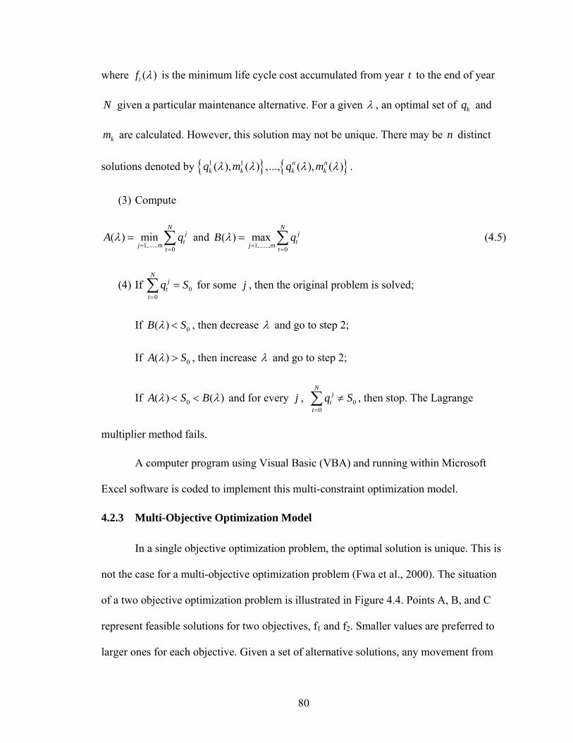
80
where ( )tf λ is the minimum life cycle cost accumulated from year t to the end of year
N given a particular maintenance alternative. For a given λ , an optimal set of kq and
km are calculated. However, this solution may not be unique. There may be n distinct
solutions denoted by { } { }1 1( ), ( ) ,..., ( ), ( )n nk k k kq m q mλ λ λ λ .
(3) Compute
1,...... 0( ) min
Nj
tj m tA qλ
==
= ∑ and 1,......, 0
( ) maxN
jtj m t
B qλ=
=
= ∑ (4.5)
(4) If 00
Nj
tt
q S=
=∑ for some j , then the original problem is solved;
If 0( )B Sλ < , then decrease λ and go to step 2;
If 0( )A Sλ > , then increase λ and go to step 2;
If 0( ) ( )A S Bλ λ< < and for every j , 00
Nj
tt
q S=
≠∑ , then stop. The Lagrange
multiplier method fails.
A computer program using Visual Basic (VBA) and running within Microsoft
Excel software is coded to implement this multi-constraint optimization model.
4.2.3 Multi-Objective Optimization Model
In a single objective optimization problem, the optimal solution is unique. This is
not the case for a multi-objective optimization problem (Fwa et al., 2000). The situation
of a two objective optimization problem is illustrated in Figure 4.4. Points A, B, and C
represent feasible solutions for two objectives, f1 and f2. Smaller values are preferred to
larger ones for each objective. Given a set of alternative solutions, any movement from

81
one solution to another that can improve at least one objective without making any other
worse off is termed a Pareto improvement. For example, moving from solution C to
solution A or solution B is a Pareto improvement. If no further Pareto improvement can
be made (i.e. moving from solution A to solution B along an indifference curve), Pareto
efficiency has been reached. The Pareto frontier is the set of choices that are Pareto
efficient.
f2
f1
A
CB
Pareto frontier
f1(A)>f1(B)
f2(A)<f2(B)
Figure 4.4 Multi-objective optimization and Pareto efficiency
Decision makers may choose different Pareto optimal solutions based on a
specific objective function. Life cycle cost and energy consumption are two important
sustainability indicators. The Pareto optimal solution for cost and energy consumption
objectives is obtained by combining the multiple objectives into one weighted objective
function as following:
Z C Eα= + (4.6)
where C is the life cycle cost, E is the life cycle energy consumption, α is the weight
factor, and Z is the weighted objective.
Variation of weight factors with the aim of minimizing the weighted objective can
be investigated. Though computationally intensive, this approach gives an idea of the
82
shape of the Pareto frontier and provides decision makers with more information about
the trade-offs among various objectives.
4.3 Pavement Asset Management System Results – Pavement Overlay Case Study
The project-level pavement asset management system integrated with multi-
objective and multi-constraint optimization models is applied to a pavement overlay
system to develop the optimal preservation strategy. Pavement overlays are the most
prevalent pavement rehabilitation method which utilizes the structure of an existing
pavement to reduce the rate of new pavement deterioration and extend pavement service
life. A common hot mixed asphalt (HMA) overlay design is analyzed. The HMA overlay
system is modeled as 10 km long freeway sections in two directions. Each direction has
two 3.6 m wide lanes, a 1.2 m wide inside shoulder, and a 2.7 m wide outside shoulder.
The thickness of the HMA overlay is 190 mm which is typical of pavement overlay
designs (Huang, 2004). In the PAMS system, the HMA overlay system is designed for a
20 year service life by the Michigan Department of Transportation (MDOT, 2005). The
annual average daily traffic (AADT) is approximately 70,000 vehicles with 8% truck
fraction (MDOT, 1997). In the baseline scenario, the annual traffic growth rate is 0%.
4.3.1 Multi-Constraint Optimization Result
Multi-constraint optimization is applied to determine optimal preservation
strategies to minimize total life cycle costs based on various preservation budget
constraints. In the analysis, the preservation budget (initial construction costs are not
included) over the 20 year pavement life is decreased from $2 million to $0.5 million
which is the minimum to keep the pavement overlay under a threshold of DI of 50

83
(MDOT, 2005). Figure 4.5 shows the impact of this budget reduction on optimal overlay
preservation strategies. As the budget decreases, expensive major maintenance activities
are replaced by numerous, lower cost, minor maintenance activities. However, this more
frequent maintenance and rehabilitation schedule associated with a lower budget
increases traffic interruptions, traffic congestion, and user delay.
2006
2011
2016
2021
2026
Overlay Construction
Minor Repair & Maintenance
Major Repair & Maintenance
$4m$1.1m $0.9m
$0.9m$0.14m $0.13m
$4m
$4m
$0.14m $0.13m $0.11m $0.10m
Initial Cost Budget: $2m
Budget: $1.2m
Budget: $0.5m
Figure 4.5 Optimal maintenance strategies based on different budget constraints
Figure 4.6 shows the total life cycle cost broken down into user cost, agency cost
and environmental cost, using the optimal preservation strategies under three budget
levels ranging from $0.5 to $2 million. As expected, agency costs decrease as the budget
constraint tightens. However, user costs, which are about 8 times higher than agency
costs over the 20 year life time of a pavement overlay system, increase as the budget
decreases. The unitless shadow prices for $2 million, $1.2 million, and $0.5 million
budget constraints are 5, 5.5, and 6, respectively.
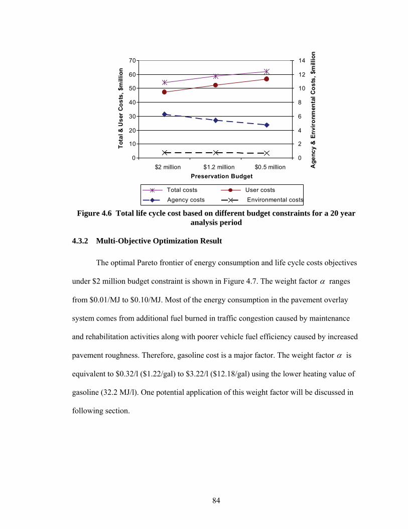
84
0
10
20
30
40
50
60
70
$2 million $1.2 million $0.5 millionPreservation Budget
Tota
l & U
ser
Cos
ts, $
mill
ion
0
2
4
6
8
10
12
14
Age
ncy
& E
nvir
onm
enta
l Cos
ts, $
mill
ion
Total costs User costsAgency costs Environmental costs
Figure 4.6 Total life cycle cost based on different budget constraints for a 20 year
analysis period
4.3.2 Multi-Objective Optimization Result
The optimal Pareto frontier of energy consumption and life cycle costs objectives
under $2 million budget constraint is shown in Figure 4.7. The weight factor α ranges
from $0.01/MJ to $0.10/MJ. Most of the energy consumption in the pavement overlay
system comes from additional fuel burned in traffic congestion caused by maintenance
and rehabilitation activities along with poorer vehicle fuel efficiency caused by increased
pavement roughness. Therefore, gasoline cost is a major factor. The weight factor α is
equivalent to $0.32/l ($1.22/gal) to $3.22/l ($12.18/gal) using the lower heating value of
gasoline (32.2 MJ/l). One potential application of this weight factor will be discussed in
following section.

85
8
9
10
11
12
13
5.8 6 6.2 6.4 6.6 6.8 7
Total life cycle cost, 107 Dollars
Tota
l ene
rgy
cons
umpt
ion,
10
8 MJ
Pareto optimal solutionOther solutionPareto frontier
Figure 4.7 Pareto frontier for total energy consumption and total life cycle cost
objectives for a 20 year analysis period
4.4 Discussion
In 2008, presidential candidates McCain and Clinton both proposed suspending
the $0.049/l ($0.184/gal) federal gas tax for 3 months during the peak summer travel
season to counteract soaring gas prices (Broder, 2008). The federal motor fuel tax is used
to partially fund the National Highway Trust Fund which is distributed to states to
maintain roads and bridges. While this tax reduction would benefit users in the short run
(Summer 2008), the long term impacts are more complex and require further analysis. In
the pavement overlay system described previously, the user tax benefit (which is also the
total 3 month gasoline tax loss for that summer due to the tax reduction plan) is:
/ //
/
70000 10 30 3 $0.049 $287,94510.7
Total Kilometer TraveledTax Reduction
Average Fuel Economy
vehicle day km days month monthl
km lUser tax benefit × × ×
= × =
6444444474444444864748
14243 (4.7)

86
In Michigan, 30% of the Highway Trust Fund is used to do pavement
rehabilitation and reconstruction (MDOT, 2007). Thus, the budget decrease would be:
$287,945 0.3 $86,384× = (4.8)
An immediate budget decrease will have a much larger impact in the future. For
example, the reduced budget will postpone necessary maintenance and rehabilitation
activities and may also force highway agencies to substitute one high-cost major
maintenance activity with several low-cost minor maintenance activities. These changes
in preservation strategy ultimately change the total life cycle cost, especially user costs.
Postponed essential maintenance and rehabilitation activities accelerate the deterioration
of pavement overlay and increase overlay surface roughness thereby adding fuel
consumption for users. More frequent minor maintenance activities interrupt normal
traffic flow and cause traffic congestion and detouring which will increase user time
delay and travel mileage. To quantify the impact of current budget constraint change on
future total life cycle cost, an average shadow price 5.5 is used.
As described previously, the shadow price, λ , is the partial derivative of total life
cycle cost with respect to agency cost. Therefore, the total life cycle cost increase
associated with this proposed plan is:
( ) $86,384 5.5 $475,109Budget change Shadow price λ× = × = (4.9)
Since 85% of total life cycle cost for a pavement overlay system is borne by users
(Zhang et al., 2008), the total user cost increase for a 3 month suspension of the federal
gasoline tax (paid over the 20 year analysis period) is:

87
85% $475,109 0.85 $287,945 $115,898Total life cycle cost User tax benefit× − = × − =
(4.10)
Conversely, if the government increases discretionary transportation budget
spending, highway agencies will have more resources to improve preservation strategies
and even promote the application of new materials and technologies. HMA is a common
material used in pavement overlay applications. However, asphalt, which is a petroleum
byproduct, poses significant environmental challenges. Additionally, the physical
limitations of asphalt, which are factors in pavement overlay failure and higher
preservation frequency, have driven the research of alternative materials, such as ECC.
ECC is a promising candidate material for road repairs, pavement overlays, and
bridge deck rehabilitation (Li, 2003). Previous research has shown that the required
thickness of an ECC overlay is half that compared to an HMA overlay while the life of an
ECC overlay is estimated to be twice that of an HMA overlay. However, the initial
construction cost of ECC overlay is higher than that of an HMA overlay. The
construction duration of an ECC overlay is also longer than an HMA overlay. The initial
construction costs and construction related congestion costs for an ECC overlay are $7
million higher to an HMA overlay ($36 million and $29 million initial costs for an ECC
overlay and an HMA overlay, respectively) (Zhang et al., 2008). If the government can
subsidize ECC for $7 million, it will make ECC material competitive with HMA material.
This subsidy will reduce the total life cycle costs by:
( ) $7,000,000 5.5 $38,500,000Budget change Shadow price λ× = × = (4.11)
An independent study of life cycle costs for an ECC and HMA overlay system
shows a similar result. The total life cycle costs of an ECC and HMA overlay system for

88
a 40 year lifetime are $48.8 million and $92.5 million, respectively. Details of life cycle
cost analysis model for each overlay system are described in Zhang et al (2008).
The multi-objective optimization analysis gives highway agencies more flexibility
to control and manage their pavement systems. Figure 4.8 shows different optimal HMA
overlay preservation strategies with a weight factor ranging from $0.32/l ($1.22/gal) to
$3.22/l ($12.18/gal) (calculated in the previous section). Generally, fuel prices reflect the
relationship between fuel demand and supply. Higher fuel price indicates the insufficient
fuel supply relative to increasing demand. Thus, at a higher fuel price, highway agencies
can adjust the preservation strategy to an energy saving strategy (higher weight factor),
which increases maintenance and rehabilitation frequency to reduce pavement surface
roughness. On the contrary, if fuel price is relatively low and economic costs are more
important, the highway agencies can focus on optimizing agencies costs, which result in
reducing maintenance and rehabilitation frequency to decrease construction related
congestion and user time delay cost.

89
2006
2011
2016
2021
2026
Overlay Construction
Minor Repair & Maintenance
Major Repair & Maintenance
α=$3.22/l($12.18/gal)
α=$0.32/l($1.22/gal)
α=$0.81/l($3.05/gal)
E=8.3×10⁸ MJ C=$6.7×10⁷
E=11.9×10⁸ MJ C =$5.9×10⁷
E=9.9×10⁸ MJ C=$6.3×10⁷
E=Total Energy ConsumptionC=Total Life Cycle Cost
Figure 4.8 Optimal maintenance strategies based on different fuel prices
4.5 Conclusion
This study demonstrates the feasibility of applying mathematical programming
methods to a pavement asset management system. A multi-constraint model and a multi-
objective model are incorporated in a project-level PAMS model to enable decision
makers to evaluate pavement infrastructure projects from a more holistic, long term
perspective while providing criteria for more sustainable infrastructure material selection.
Multi-constraint and multi-objective analysis provides a quantitative base for
pavement preservation policy making. The results of multi-constraint analysis show that
the total life cycle cost of an HMA overlay system increases from $54 million to $61
million as the agency budget decreases from $2 million to $0.5 million. Suspending the
gas tax will not benefit highway users from a long term perspective. The shadow price of
the HMA overlay system shows that a $0.29 million suspension of the gas tax for 3
months will cost about $0.40 million to highway users over 20 year period. Additionally,
a government subsidy can be helpful to promote the application of new materials and

90
technologies which can further decrease life cycle costs compared to those of
conventional low initial cost techniques. A $7 million subsidy to implement ECC overlay
technologies can reduce life cycle costs by $38.5 million in the future.
Multi-objective optimization enables highway agencies to develop their
preservation strategy based on weighted objectives to achieve maximized benefit. A
series of weight factors between energy consumption and life cycle cost objectives are
generated. These weight factors are converted to fuel prices ranging from $0.32/l
($1.22/gal) to $3.22/l ($12.18/gal). At a higher fuel price, a more frequent preservation
strategy that decreases pavement surface roughness and saves energy is preferred. If the
fuel price is relatively low, decreasing the pavement maintenance and rehabilitation
frequency will decrease the user time delay caused by construction activities and then
decrease the total life cycle cost.
The multi-constraint and multi-objective optimization models developed here
represent a new set of tools to guide policy making that can enhance transportation
infrastructure sustainability.

91
References
Ahmed, K., Abu-Lebdeh, G., and Lyles, R. W. (2006). “Prediction of pavement distress index with limited data on causal factors: an auto-regression approach.” The International Journal of Pavement Engineering, 7(1), 23-35.
American Society of Civil Engineering (ASCE). (2005) http://www.asce.org/reportcard/2005/index2005.cfm
American Society of Civil Engineering (ASCE). (2006) Road to Infrastructure Renewal—A Voter’s Guide, Reston, Va.
Broder, J. M. (2008) Democrats divided over gas tax break. The New York Times, April 29, 2008.
Dreyfus, S. F., and Law, A. M. (1977) The Art and Theory of Dynamic Programming. Academic Press, New York, NY.
Fwa, T. F., Chan, W. T., and Hoque, K. Z. (2000). “Multiobjective optimization for pavement maintenance programming.” Journal of Transportation Engineering, 126(5), 363-374.
Golabi, K., Kulkarni, R. B., and Way, G. B. (1982). “A statewide pavement management system.” Interfaces, 12, 5-21.
Huang, Y. H. (2004) Pavement analysis and design. University of Kentucky, Upper saddle River, NJ.
Kendall, A., Keoleian, G. A., and Helfand, G. (2008) “Integrated life-cycle assessment and life-cycle cost analysis model for concrete bridge deck applications.” Journal of Infrastructure Systems, 14 (3), 214-222.
Keoleian, G. A., Kendall, A., Dettling, J. E., Smith, V. M., Chandler, R. F., Lepech, M. D., and Li, V. C. (2005). “Life cycle modeling of concrete bridge design: Comparison of engineered cementitious composite link slabs and conventional steel expansion joints.” Journal of infrastructure systems, 11(1), 51-60.
92
Keoleian, G. A. and Spitzley, D.V. (2006). “Life Cycle Based Sustainability Metrics.” Chapter 7 in Sustainability Science and Engineering: Defining Principles (Sustainability Science and Engineering, Volume 1), M.A. Abraham, Ed. Elsevier, pp. 127-159.
Kim, H. C., Keoleian, G. A., Grande, D. E., and Bean, J. C. (2003). “Life cycle optimization of automobile replacement: Model and application.” Environmental Science and Technology, 37, 5407-5413.
Li, V. C. (2003). “Durable overlay systems with engineered cementitious composites (ECC).” International Journal for Restoration of Buildings and Monuments, 9(2), 1-20.
Mbwana, J. R. (2001). “A framework for developing stochastic multi-objective pavement management system.” Technology Transfer in Road Transportation in Africa, Arusha, Tanzania.
Michigan Department of Transportation (MDOT). (1997) 1997 Noninterstate freeway segments: Deficient segments-URBAN. Ann Arbor, Michigan.
Michigan Department of Transportation (MDOT). (2005) Pavement desigan and selection manual. Ann Arbor, Michigan.
Michigan Department of Transportation (MDOT). (2007) Five-Year transportation program. Ann Arbor, Michigan.
Qian, S. (2007) Influence of concrete material ductility on the behavior of high stress concentration zones. Doctoral thesis. University of Michigan, Ann Arbor, Michigan.
Wilde, W. J., Waalkes, S., and Harrison, R. (2001) Life cycle cost analysis of Portland cement concrete pavement, University of Texas at Austin, Austin, Texas.
Zhang, H., Keoleian, G. A., and Lepech, M. D. (2008). An integrated life cycle assessment and life cycle analysis model for pavement overlay systems. First International Symposium on Life-Cycle Civil Engineering, Varenna, Italy, pp. 907-915.

93
Zhang, H., Lepech, M. D., Keoleian, G. A., Qian, S. Z., and Li, V. C. (2009). “Dynamic life cycle modeling of pavement overlay systems: capturing the impacts of users, construction, and roadway deterioration.” To be submitted to Journal of Infrastructure Systems.

94
CHAPTER 5
NETWORK-LEVEL PAVEMENT ASSET MANAGEMENT SYSTEM INTEGRATED WITH LIFE CYCLE ANALYSIS AND LIFE CYCLE
OPTIMIZATION
ABSTRACT
A network-level pavement asset management system (PAMS) utilizing life cycle
analysis and life cycle optimization methods was developed. Three priority selection
methods were developed based on benefit, benefit cost ratio, and binary integer
programming to allocate the limited preservation budget. A geographic information
system (GIS) model was utilized to enhance the network-level PAMS by collecting,
managing, and visualizing pavement condition data. The new network-level pavement
asset management system allows decision makers to preserve a healthy pavement
network and minimize total life cycle cost, while also meeting budget constraints and
other agency constraints. A case study application to Washtenaw County, Michigan,
compared the optimal preservation strategies with the Michigan Department of
Transportation’s current preservation practice. The results show that the optimal
preservation strategies can reduce total life cycle cost by 9%-13% compared to the
current preservation plan. The impact of annual preservation budget on total life cycle
cost was analyzed. A $3 million annual preservation budget reduction will significantly
increase user costs by $450 million for a 40 year analysis period.
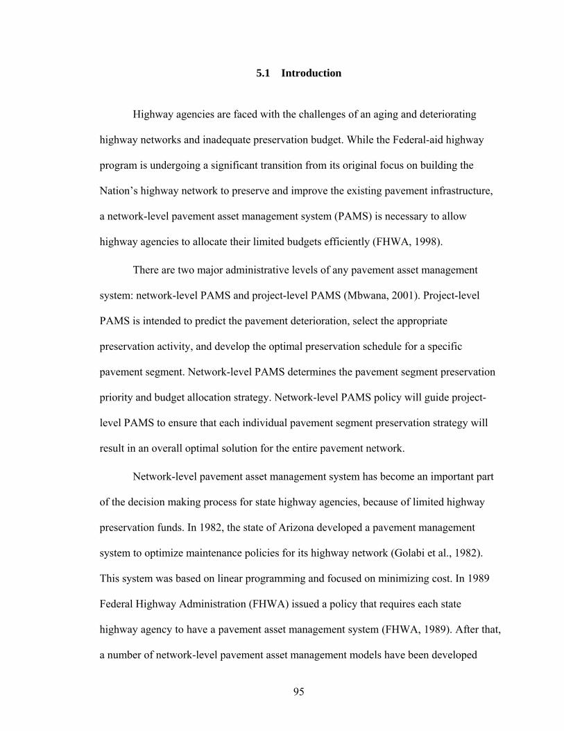
95
5.1 Introduction
Highway agencies are faced with the challenges of an aging and deteriorating
highway networks and inadequate preservation budget. While the Federal-aid highway
program is undergoing a significant transition from its original focus on building the
Nation’s highway network to preserve and improve the existing pavement infrastructure,
a network-level pavement asset management system (PAMS) is necessary to allow
highway agencies to allocate their limited budgets efficiently (FHWA, 1998).
There are two major administrative levels of any pavement asset management
system: network-level PAMS and project-level PAMS (Mbwana, 2001). Project-level
PAMS is intended to predict the pavement deterioration, select the appropriate
preservation activity, and develop the optimal preservation schedule for a specific
pavement segment. Network-level PAMS determines the pavement segment preservation
priority and budget allocation strategy. Network-level PAMS policy will guide project-
level PAMS to ensure that each individual pavement segment preservation strategy will
result in an overall optimal solution for the entire pavement network.
Network-level pavement asset management system has become an important part
of the decision making process for state highway agencies, because of limited highway
preservation funds. In 1982, the state of Arizona developed a pavement management
system to optimize maintenance policies for its highway network (Golabi et al., 1982).
This system was based on linear programming and focused on minimizing cost. In 1989
Federal Highway Administration (FHWA) issued a policy that requires each state
highway agency to have a pavement asset management system (FHWA, 1989). After that,
a number of network-level pavement asset management models have been developed
96
during the past two decades. Mbwana used Markov decision model to predict pavement
network condition and applied linear programming to determine the optimal pavement
maintenance and rehabilitation strategy (Mbwana and Turnquist, 1996). Chootinan et al.
developed a network-level pavement maintenance program using genetic algorithm to
maximize pavement performance and minimize pavement maintenance cost (Chootinan
et al., 2006). Currently, the Michigan Department of Transportation (MDOT) relies on
the Michigan Road Quality Forecasting System (RQFS) to develop preservation
strategies for regional DOT management districts. This software uses current pavement
condition data from their pavement management system to predict future network
conditions at different levels of investment. However, to improve sustainability, modern
pavement asset management systems should also have the ability to account for other
sustainability indicators, such as user time delay caused by preservation activities,
additional fuel consumption caused by pavement surface deterioration, and
environmental impacts. Life cycle assessment (LCA) and life cycle cost analysis (LCCA)
have been identified as the most comprehensive tools to evaluate sustainability
performance (Keoleian and Spitzley, 2006; Zhang et al., 2008).
Another challenge in developing a network-level PAMS is the ability of
managing and analyzing the large pavement condition dataset. A network-level PAMS
relies on pavement condition information for identifying pavement construction sections,
developing preservation strategy, and allocating budget. Geographic information system
(GIS), with its unique spatial analysis capability, allows highway agencies to integrate,
manage, query, and visualize pavement conditions. A number of researchers and highway
agencies have applied GIS platform for enhancing pavement asset management. Medina
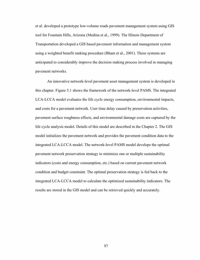
97
et al. developed a prototype low-volume roads pavement management system using GIS
tool for Fountain Hills, Arizona (Medina et al., 1999). The Illinois Department of
Transportation developed a GIS based pavement information and management system
using a weighted benefit ranking procedure (Bham et al., 2001). These systems are
anticipated to considerably improve the decision making process involved in managing
pavement networks.
An innovative network-level pavement asset management system is developed in
this chapter. Figure 5.1 shows the framework of the network-level PAMS. The integrated
LCA-LCCA model evaluates the life cycle energy consumption, environmental impacts,
and costs for a pavement network. User time delay caused by preservation activities,
pavement surface roughness effects, and environmental damage costs are captured by the
life cycle analysis model. Details of this model are described in the Chapter 2. The GIS
model initializes the pavement network and provides the pavement condition data to the
integrated LCA-LCCA model. The network-level PAMS model develops the optimal
pavement network preservation strategy to minimize one or multiple sustainability
indicators (costs and energy consumption, etc.) based on current pavement network
condition and budget constraint. The optimal preservation strategy is fed back to the
integrated LCA-LCCA model to calculate the optimized sustainability indicators. The
results are stored in the GIS model and can be retrieved quickly and accurately.
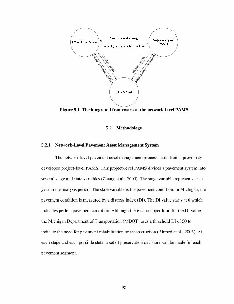
98
Initia
lize
pave
men
t net
work
Visu
alize
resu
ltsProvide pavem
ent condition
Visualize results
Figure 5.1 The integrated framework of the network-level PAMS
5.2 Methodology
5.2.1 Network-Level Pavement Asset Management System
The network-level pavement asset management process starts from a previously
developed project-level PAMS. This project-level PAMS divides a pavement system into
several stage and state variables (Zhang et al., 2009). The stage variable represents each
year in the analysis period. The state variable is the pavement condition. In Michigan, the
pavement condition is measured by a distress index (DI). The DI value starts at 0 which
indicates perfect pavement condition. Although there is no upper limit for the DI value,
the Michigan Department of Transportation (MDOT) uses a threshold DI of 50 to
indicate the need for pavement rehabilitation or reconstruction (Ahmed et al., 2006). At
each stage and each possible state, a set of preservation decisions can be made for each
pavement segment.
99
A burden function ( , )B i j is defined as the current burden (energy consumption,
GHG emissions, or total cost) caused by a certain preservation activity for a specific
pavement segment. The burden function can be described by Equation 5.1.
( , ) ( , ) ( , ) ( , ) ( , ) ( , ( )) 0( , )
0 0M C D CG E UB i j B i j B i j B i j B i j B i DI i if i
B i jif i
+ + + + + >⎧= ⎨ =⎩
(5.1)
where i is the current stage (year), j is the preservation alternative, ( , )MB i j is the
burden associated with the material module at year i with decision j . Similarly, ( , )CB i j ,
( , )DB i j , ( , )CGB i j , and ( , )EB i j are the burdens of construction, distribution, traffic
congestion, and end of life processes, respectively, at year i with decision j .
( , ( ))UB i DI i is the burden of pavement usage which is caused by pavement surface
roughness effects at year i with a particular distress index.
A backward dynamic programming procedure was developed to select the optimal
preservation strategy from all candidate decisions (Zhang et al., 2009).
If the highway agency has enough budget, all segments in the pavement network
should follow the optimal preservation strategy developed by the project-level PAMS to
achieve the optimal results (minimizing life cycle energy consumption, environmental
impacts, or costs). However, if the total budget of the highway agency cannot cover the
entire pavement network, the network-level PAMS is necessary to adjust the optimal
preservation strategy developed from the project-level PAMS and allocate the limited
budget to specific pavement segments based on a priority selection process. Thus, priority
selection model is the key part in the network-level PAMS.

100
5.2.2 Priority Selection Model
To decide the priority of each pavement segment, three selection methods are
developed. The first method is based on benefit. Benefit is defined as ( , 0) ( , )B i B i j− ,
where ( , 0)B i is the current burden without applying any preservation activity at year i
and ( , )B i j is the current burden with applying preservation activity j at year i . If
applying preservation activity j to pavement segment k has a larger benefit than the
benefit of applying the same preservation activity to the other pavement segments,
pavement segment k will have a higher priority to do preservation activity j . The
second method is based on benefit cost ratio. The benefit cost ratio is defined as
( ( , 0) ( , )) / ( , )B i B i j C i j− , where ( , )C i j is the agency cost of preservation activity j at
year i . Similarly, if applying preservation activity j to pavement segment k has a larger
benefit cost ratio than the benefit cost ratio of applying the same preservation activity to
the other pavement segments, pavement segment k will have a higher priority to do
preservation activity j .
However, these two methods are not based on mathematical programming. They
may not always identify the global optimal result. To solve this problem, a third method
is developed based on binary integer programming. The objective is to minimize the
overall burden for the entire pavement network at year i . So the objective function is
defined as:
Minimize 1 1 2 2 ......T T Tn nB X B X B X+ + + (5.2)
where [ ]1 2, ,......,k k k kmB b b b= and [ ]1 2, ,......k k k kmX x x x= . kB is the burden matrix of
pavement segment k , from current state to the last state; kX is the preservation activity

101
matrix of pavement segment k . T means transpose. kjb is the burden of doing
preservation activity j of pavement segment k , from current state to the last state ; kjx is
the preservation activity j of pavement segment k .
Subject to:
1 1 2 2 ......T T Tn nC X C X C X C+ + + ≤ (5.3)
where [ ]1 2, ,......,k k k kmC c c c= . kC is the agency cost matrix of pavement segment k , C
is the total annual budget. kjc is the agency cost of preservation activity j of pavement
segment k .
Also, the other constraints include:
(50)DI Max DI≤ (5.4)
0, 1, 2,......, ; 1, 2,......,kjx k n j m≥ = = (5.5)
int, 1, 2,......, ; 1, 2,......,kjx k n j m∈ = = (5.6)
1
1, 1, 2,......,m
kjj
x k n=
= =∑ (5.7)
A computer program using Visual Basic Application (VBA) and running within
Microsoft Excel software was coded to implement the priority selection model and link it
to the network-level PAMS. Three network-level pavement asset management systems
based on benefit, benefit cost ratio, and binary integer programming selection methods
are developed and named as PAMS1, PAMS2, and PAMS3, respectively.

102
5.2.3 GIS Model
To integrate GIS application with the network-level pavement asset management
system, several GIS base map layers are created which contain multiple sets of attributes.
Attributes are data in digital map layer that are linked to linear pavement features, such as
control section (CS), pavement type (concrete or asphalt), pavement remaining service
life (RSL), annual average daily traffic (AADT) and commercial average daily traffic
(CADT), and pavement condition (distress index). Linear referencing method provides an
intuitive way to associate these attributes to the portions of pavements. These attributes
can be further displayed, queried, edited, and analyzed without affecting the underlying
linear feature’s geometry (ESRI, 2004). In linear referencing, a route is created to model
the linear feature using a one-dimensional measuring system. The measuring system
records the data by using a relative position along an already existing linear pavement
feature. For example, route US-23, kilometer point 11.5, uniquely identifies a position in
a map without using two-dimensional (x, y) geographic coordinates. Route event tables
are used to store linearly referenced attributes. Event table is a relational database
management system table supported by GIS platform. Because events simply reference
measure locations along linear features, they are edited and maintained independently of
the pavement features. Event rows are composed of a route identifier, measure values
indicating a location, and one or more attributes associated with the location. As shown in
Figure 5.2, along a route, beginning and ending meter points (BMP and EMP,
respectively) of different attributes rarely match. To generate the final pavement
segments and visualize them on map, a dynamic segmentation method is used.

103
Control Section
Pavement Type
RSL
Traffic Flow
Distress Index
Final Segment
0 10 20 40 km Figure 5.2 Route event segmenting process
Dynamic segmentation is a process of computing the map location of events
stored in an event table and allows multiple sets of attributes to be associated with any
portion of a linear feature. Figure 5.3 shows how the dynamic segmentation method
overlays two route event tables to produce a single route event table. The route event
table (a) stores traffic flow information (AADT). The route event table (b) stores
pavement condition data (DI). The two event tables are unioned to a third event table.
The output event table (c) contains all of the input events, which have been split where
they intersected.

104
7.9379132198104119.03219160981041
101609081062
25.41609081041
214828160981062
DIEMPBMPCS
7.9379132198104119.03219160981041
101609081062
25.41609081041
214828160981062
DIEMPBMPCS
559003219081062624004828321981062
AADTEMPBMPCS
700003791321981041856003219081041
559003219081062624004828321981062
AADTEMPBMPCS
700003791321981041856003219081041
2121107.919.025.4DI
559001609081062
6240055900
700008560085600AADT
37913219810413219160981041
3219160981062
1609081041
4828321981062
EMPBMPCS
2121107.919.025.4DI
559001609081062
6240055900
700008560085600AADT
37913219810413219160981041
3219160981062
1609081041
4828321981062
EMPBMPCS
(a) (b)
(c)
Figure 5.3 Union of two route event tables using dynamic segmentation
The commercially available GIS software ArcGIS 9.2 has been used to create the
digital pavement network map and conduct the linear referencing process. A Visual Basic
program is developed to implement data transfer between ArcGIS and network-level
PAMS.
5.3 Case Study: Washtenaw County Pavement Network
5.3.1 Pavement Network Initialization
Washtenaw County, Michigan, was selected for the case study. Washtenaw
County covers 1,871 km2 and has almost 350,000 residents (Census Bureau, 2008).
Several major highways cross Washtenaw County, including I-94 (Interstates), US-23
(US highways), and M-14 (Michigan State Trunklines). The pavements in Washtenaw
County are preserved by the Michigan Department of Transportation. They also collect
and maintain the pavement information data. These data provide the length, width,
location, pavement type, pavement distress index, and traffic flow of each pavement.

105
Query analysis is conducted in the GIS model for identification of the pavement sections
which satisfy the following predefined intervention criteria:
(a) All pavement sections are freeways
(b) AADT ≥ 30000
(c) CADT ≥ 4000
Linear referencing and dynamic segmentation methods are applied to the initial
dataset. A total number of 32 pavement segments (total 120 km long) are generated. The
description of each pavement segment is listed in Table 5.1.

106
Table 5.1 Pavement segments information list
ID Name CS BMP EMP Type AADT CADT RSL DI 1 I-94 81041 0 3790.8 Concrete 85233 9200 10 17.4 2 I-94 81062 0 4828.0 Asphalt 55900 7900 12 15.5 3 I-94 81062 4828.0 11265.4 Asphalt 70650 7900 12 11.6 4 I-94 81062 11265.4 14661.0 Asphalt 85433 8633 9 3.9 5 I-94 81063 0 3128.7 Asphalt 106900 11600 9 2.0 6 I-94 81063 3128.7 4828.0 Asphalt 103500 11600 3 2.0 7 I-94 81063 4828.0 5809.6 Asphalt 103500 11600 7 6.4 8 US-23 81074 0 6437.4 Concrete 73850 6950 6 9.3 9 US-23 81074 6437.4 12028.0 Concrete 70500 6900 6 4.1 10 M-14 81075 0 1810.0 Concrete 56100 5500 11 25.3 11 US-23 81075 0 4828.0 Asphalt 64300 6000 11 21.1 12 US-23 81075 4828.0 11748.2 Asphalt 65820 6000 11 20.0 13 US-23 81075 0 1209.8 Asphalt 63100 7900 11 24.5 14 US-23 81076 0 1609.3 Concrete 36900 6300 12 9.4 15 US-23 81076 1609.3 11265.4 Asphalt 41817 6300 7 13.2 16 US-23 81076 11265.4 15922.9 Asphalt 57233 6833 8 16.8 17 M-14 81103 0 1609.3 Asphalt 70100 6900 13 5.8 18 M-14 81103 1609.3 4828.0 Asphalt 63600 5500 7 13.9 19 M-14 81103 4828.0 6437.4 Asphalt 63600 5500 16 4.1 20 M-14 81103 6437.4 8046.7 Asphalt 62200 5500 9 8.3 21 M-14 81103 8046.7 9656.1 Asphalt 62200 5500 1 9.8 22 M-14 81103 9656.1 11265.4 Asphalt 62200 5500 4 8.6 23 M-14 81103 11265.4 12874.8 Asphalt 62200 5500 6 5.6 24 M-14 81103 12874.8 13850.0 Asphalt 61700 5500 8 5.2 25 I-94 81104 0 9656.1 Asphalt 49067 8600 7 6.1 26 I-94 81104 9656.1 19312.1 Asphalt 55500 9200 3 21.1 27 I-94 81104 19312.1 28968.2 Asphalt 61050 8983 7 9.3 28 I-94 81104 28968.2 29396.3 Asphalt 46600 7900 12 5.7 29 M-14 81105 0 5886.9 Concrete 32750 4400 3 1.7 30 US-23 81103 0 1609.3 Concrete 63100 7900 7 9.1 31 US-23 81103 1609.3 3128.7 Concrete 63100 7900 11 3.6 32 US-23 81103 3128.7 3863.0 Concrete 63100 7900 10 3.2

107
Figure 5.4 shows the GIS map and the initial pavement network condition.
Figure 5.4 GIS map and pavement network condition
5.3.2 Network-level pavement asset management results
The network-level PAMS is applied to the above pavement network to develop
the optimal preservation strategy for a 40 year analysis period. The annual budget for the
entire pavement network is derived from the Michigan Five-Year Transportation Program
(MDOT, 2007). In the 2007 to 2011 Five-Year Transportation Program, Washtenaw
County and other nine nearby counties can receive approximately $368 million for 2,150
km road preservation. The annual budget allocated to the pavement network in this
research is estimated to be $4 million/year.
Alternative preservation methods used in this research are defined in the
Michigan Pavement Design and Selection Manual (MDOT 2005). The unit costs are
shown in Table 5.2.

108
Table 5.2 Alternative preservation methods and unit costs
Method Unit cost, $/lane-km Do nothing 0 Minor Maintenance 4000-5000 Major Maintenance 28750-36250 Overlay 106550-106860
Using the network-level PAMS, 3 sets of optimal preservation strategies based on
the three priority selection methods (PAMS1, PAMS2, and PAMS3) are developed.
Another case based on the MDOT preservation plan is also generated to compare to the
optimal preservation strategies. Figure 5.5 shows the pavement surface condition which
is represented by the distress index in the 40 year analysis period using different
preservation strategies. Due to allocate the resource efficiently, the pavement surface
conditions of preservation strategies using PAMS1, PAMS2, and PAMS3 methods are
generally better than the conditions of MDOT plan. This better pavement surface
condition will decrease the fuel consumption for highway drivers and decrease the user
fuel costs.
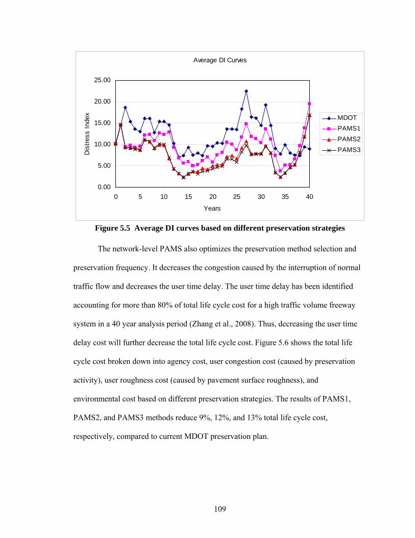
109
Average DI Curves
0.00
5.00
10.00
15.00
20.00
25.00
0 5 10 15 20 25 30 35 40
Years
Dis
tress
Inde
x MDOTPAMS1PAMS2PAMS3
Figure 5.5 Average DI curves based on different preservation strategies
The network-level PAMS also optimizes the preservation method selection and
preservation frequency. It decreases the congestion caused by the interruption of normal
traffic flow and decreases the user time delay. The user time delay has been identified
accounting for more than 80% of total life cycle cost for a high traffic volume freeway
system in a 40 year analysis period (Zhang et al., 2008). Thus, decreasing the user time
delay cost will further decrease the total life cycle cost. Figure 5.6 shows the total life
cycle cost broken down into agency cost, user congestion cost (caused by preservation
activity), user roughness cost (caused by pavement surface roughness), and
environmental cost based on different preservation strategies. The results of PAMS1,
PAMS2, and PAMS3 methods reduce 9%, 12%, and 13% total life cycle cost,
respectively, compared to current MDOT preservation plan.

110
0
500
1000
1500
2000
MDOT PAMS1 PAMS2 PAMS3
Life
cyc
le c
ost,
$mill
ion
EnvironmentUser RoughnessUser CongestionAgency
Figure 5.6 Total life cycle cost of different preservation strategies
Annual preservation budget is an important factor which determines the total
resource that the highway agency can use for pavement preservation. To identify the
impact of annual preservation budget on total life cycle cost, a sensitivity analysis is
conducted using PAMS3 method. The result is shown in Figure 5.7. While the annual
budget decreases from $4 million to $1 million, the total life cycle cost (present value)
increases from $1310 million to $1690 million over a 40 year service life. As expected,
agency costs decrease as the budget constraint tightens. However, user congestion cost
and user roughness cost, which combined are about 8 times higher than agency costs over
the 40 year life time of a pavement overlay system, increase as the annual preservation
budget decreases. The model indicates that for a budget less than $1 million/yr is not
enough to preserve the entire pavement network without failure (DI > 50).

111
0
250
500
750
1000
1250
1500
1750
2000
$4 million $3 million $2 million $1 million
Annual Preservation Budget
Use
r Con
gest
ion
& T
otal
Life
Cyc
leC
osts
, $m
illio
n
0
50
100
150
200
250
300
350
400
Age
ncy,
Use
r Rou
ghne
ss, a
nd
Env
. Cos
ts, $
mill
ion
Total User Congestion Agency User Roughness Environment
Figure 5.7 Total life cycle cost based on different annual budget
The results obtained through network-level pavement asset management system
have been imported to the GIS model and visualized on the digital map created before.
Figure 5.8 shows an example of the different attributes illustrated on the map. All other
attributes associated with any pavement section can be selected and visualized on the
graphical map.

112
Figure 5.8 Visualization of different attributes in GIS map
5.4 Conclusion
This study describes the development of a network-level pavement asset
management system (PAMS) that integrates life cycle analysis, optimization, and GIS. In
the network-level PAMS model life cycle analysis captures user congestion cost, user
roughness cost, and environmental costs as well as agency costs. Life cycle optimization
is applied to determine the optimal preservation strategy for a pavement network and to
minimize total life cycle cost within an analysis period. Three priority selection methods
are developed based on different criteria to allocate the limited budget efficiently. Binary
integer programming performed more accurately than the other methods in this research
to reach a global optimal budget allocation result.

113
A GIS model and interface was developed to enhance the network-level pavement
asset management system by collecting, managing, and visualizing pavement condition
data. Query analysis was conducted in the GIS model to identify the specific pavement
network in the basic digital map. Linear referencing and dynamic segmentation methods
are applied to define the pavement segment and associate pavement information with any
pavement portion. GIS model integrated with the network-level PAMS provides a unique
way to immediately retrieve and visualize all pavement network attributes, such as
pavement condition, current pavement preservation activity, and costs, on the graphical
map. This unique function enables more effective communication between highway
agencies and preservation strategy development.
The case study application to Washtenaw County, Michigan, demonstrated the
capability of the PAMS to improve preservation performance. The result showed that the
optimal preservation strategies can reduce total life cycle cost by 9%-13% compared to
preservation practice used by the Michigan Department of Transportation. Since LCCA
has been required by MDOT in the design of all projects with paving costs greater than
$1 million since 1998, the improvement of optimal preservation strategies is limited.
However, MDOT preservation plan can not anticipate the impacts of constraints changes
and dynamically adjust the preservation strategy. Annual preservation budget has
significant impact on total life cycle cost. A preservation budget reduction from $4
million/yr to $1 million/yr increases the total life cycle cost from $ 1310 million to $1690
million. It is expected that greater benefits might be realized in states that don’t employ
LCCA. In the present application of the PAMS model, the annual budget was fixed but
the model can also be implemented with a variable budget constraints for a given analysis

114
period. Furthermore, with the flexibility of life cycle analysis and life cycle optimization,
the pavement asset management system developed in this research can be scaled up to
larger pavement networks.
115
References
Ahmed, K., Abu-Lebdeh, G., and Lyles, R. W. (2006). “Prediction of pavement distress index with limited data on causal factors: an auto-regression approach.” The International Journal of Pavement Engineering, 7(1), 23-35.
Bham, G. H., Gharaibeh, N. G., and Darter, M. I. (2001) Developemtn of GIS-based Illinois highway pavement management system. ESRI User Conference, Sna Diego, California.
Chootinan, P., Chen, A., and Horrocks, M. R. et al. (2006). “A multi-year pavement maintenance program using a stochastic simulation-based genetic algorithm approach.” Transportation Research Part A, 40, 725-743.
ESRI. (2004) Linear referencing in ArcGIS. Redlands, California.
Federal Highway Administration (FHWA). (1989) Pavement policy for highways. Federal Register. Final Rule. Docket No. 87-16. Kansas City, Missouri.
Federal Highway Administration (FHWA). (1998) Pavement preservation: a road map for the future. Kansas City, Missouri.
Golabi, K., Kulkarni, R. B., and Way, G. B. (1982). “A statewide pavement management system.” Interfaces, 12, 5-21.
Keoleian, G. A. and Spitzley, D.V. (2006). “Life Cycle Based Sustainability Metrics.” Chapter 7 in Sustainability Science and Engineering: Defining Principles (Sustainability Science and Engineering, Volume 1), M.A. Abraham, Ed. Elsevier, pp. 127-159.
Mbwana, J. R. and Turnquist, M. A. (1996). “Optimization modeling for an enhanced network-level pavement management system.” Transportation Research Record, 1542, 76-85
Mbwana, J. R. (2001). “A framework for developing stochastic multi-objective pavement management system.” Technology Transfer in Road Transportation in Africa, Arusha, Tanzania.
116
Medina, A., Flintsch, G. W., and Zaniewski, J. P. (1999). “Geographic information systems-based pavement management system.” Transportation Research Record, 1652, 151-157.
Michigan Department of Transportation (MDOT). (2005) Pavement desigan and selection manual. Ann Arbor, Michigan.
Michigan Department of Transportation (MDOT). (2007) Five-Year transportation program. Ann Arbor, Michigan.
U.S. Census Bureau. (2008) http://quickfacts.census.gov/qfd/states/26/26161.html
Zhang, H., Keoleian, G. A., and Lepech, M. D. (2008). “An integrated life cycle assessment and life cycle analysis model for pavement overlay systems.” First International Symposium on Life-Cycle Civil Engineering, Varenna, Italy, pp. 907-915.
Zhang, H., Lepech, M. D., Keoleian, G. A., Qian, S. Z., and Li, V. C. (2009). “Dynamic life cycle modeling of pavement overlay systems: capturing the impacts of users, construction, and roadway deterioration.” To be submitted to Journal of Infrastructure Systems.

117
CHAPTER 6
CONCLUSIONS AND FUTURE WORK
6.1 Conclusions
This dissertation has focused on the development of a new framework for
evaluating and enhancing the sustainability of pavement systems from alternative
material applications, asset management, and policy making perspectives. Ultimately this
has produced a unique collaborative platform upon which a variety of analysis methods
and tools including life cycle analysis, life cycle optimization, microeconomics, decision
making, and spatial analysis interface with the overall goal of improving infrastructure
system sustainability. The new methods enable decision makers to evaluate and preserve
pavement systems from a more comprehensive, long term perspective and provide
criteria for more sustainable infrastructure material selection.
Four main research activities have been divided into individual chapters
depending upon their objectives: life cycle assessment and life cycle cost analysis model
evaluating the sustainability indicators of pavement systems and comparing new designs
and ECC materials to conventional designs and materials; project-level pavement asset
management system optimizing the pavement preservation strategy and improving the
sustainability; multi-objective and multi-constraint optimization model exploring the
impact of policies based on the project-level PAMS; and finally, the network-level

118
pavement asset management system applied to a pavement network minimizing life cycle
cost, while also meeting budget constraints and other agency constraints. Significant
findings and accomplishments made in individual research tasks are summarized in the
following.
6.1.1 Development of the Integrated Life Cycle Assessment and Life Cycle Cost
Analysis Model
Chapter 2 focused on the development of life cycle analysis framework. An
integrated life cycle assessment and life cycle cost analysis model was developed to
compare the sustainability of an unbonded concrete overlay system, a hot mixed asphalt
overlay system, and an ECC overlay system. The model captures cumulative traffic flows,
overlay deterioration over time, and preservation activities to evaluate life cycle energy
consumption, environmental impacts, and costs. The incorporation of pavement overlay
roughness effects on fuel consumption and related life cycle environmental burdens
represents a significant extension of existing models. Without considering roughness
effect, the life cycle energy consumption of concrete, ECC, and HMA overlay systems
will decrease 23%, 36%, and 14%, respectively (traffic condition and other system
parameters were defined in Chapter 2).
The model results showed that the overlay application of ECC material may
effectively reduce the total life cycle energy consumption, environmental impacts, and
costs when compared to the conventional materials and designs. While ECC is more
energy and cost intensive per unit volume, compared to the concrete and HMA overlay
systems, model results indicate the ECC overlay system reduces the total life cycle
energy by 15% and 72%, greenhouse gas (GHG) emissions by 32% and 37%, and costs

119
by 40% and 58% over the entire 40 year life cycle, respectively. These advantages are
derived from the expected enhanced material properties of ECC which should prevent
reflective cracking failures. While the assumption of longer service life of the ECC
overlay system is supported by results of experimental tests, FEM simulations, and bridge
deck applications, it is necessary to verify the result with the actual application of ECC
material in an overlay system and observation of its performance over time.
The analysis also showed the potential of environmentally preferable mixtures
which use industrial byproduct as a substitute for energy intensive materials, such as
using waste fly ash to replace portions of Portland cement in the ECC overlay system.
This substitution results in significantly reduced raw material and energy consumption
and decreased environmental burdens while maintaining or improving overlay system
performance.
Material consumption, traffic congestion caused by construction activities, and
pavement surface roughness effects caused by overlay deterioration are identified as three
dominant factors that influence the energy consumption, environmental impacts, and
costs of overlay systems. These three factors are determined by the pavement
preservation strategy. This result led to the following research on searching for the
optimal pavement maintenance and rehabilitation strategy to minimize life cycle energy
consumption, environmental impacts, and costs.
6.1.2 Project-Level Pavement Asset Management System
Chapter 3 focused on the development of a project-level pavement asset
management system. The project-level PAMS which determines an optimal pavement
preservation strategy is identified through the application of life cycle optimization and

120
dynamic programming tools for modeling the sustainability indicators and breaking the
complicated system into several sub processes. The integration of modern optimization
techniques and life cycle analysis methods improves the management capability of
transportation agencies as compared to current pavement asset management practice.
The project-level pavement asset management system is applied to the ECC,
concrete, and HMA overlay systems. The results show that the optimal preservation
strategies will reduce the total life cycle energy consumption by 5%-30%, the GHG
emissions by 4%-40%, and the costs by 0.4%-12% for three overlay systems compared to
current the Michigan Department of Transportation preservation strategies. Total life
cycle costs of MDOT strategies have been controlled nearly to the optimal levels,
because LCCA and user costs have been incorporated into their design.
The importance of optimizing maintenance and rehabilitation strategy in future
years proved to be even more critical when the uncertainty of future traffic condition was
considered. MDOT’s pavement preservation strategies cannot model traffic flow changes.
Results show that the preservation strategy is highly sensitive to traffic flow. With a 2%
annual traffic growth rate, the optimal preservation strategies show greater advantages
when compared to MDOT preservation strategies. Due to improved material properties
and extended service life, at higher traffic growth rates, the ECC overlay system shows
superior advantages in energy consumption, GHG emissions, and cost, compared to the
concrete overlay system and HMA overlay system.
The trade-offs between material consumption, traffic congestion, and pavement
surface roughness effects are identified in this research. Energy consumption
minimization leads to a more frequent preservation strategy, while cost minimization
121
favors a less frequent preservation strategy. This conflicting result on optimal
preservation strategy selection highlighted the necessity to implement a more
comprehensive optimization model.
6.1.3 Multi-Objective and Multi-Constraint Optimization in Project-Level
Pavement Asset Management
Chapter 4 investigated the impact of pavement preservation policies. The multi-
constraint model and a multi-objective model were incorporated in the project-level
PAMS to provide a quantitative base for policy development. A case study of a hot mixed
asphalt overlay system shows that a reduction in total agency preservation budget from
$2 million to $0.5 million increases the total life cycle cost from $54 million to $61
million over a 20 year service life. The shadow prices of the HMA overlay system
derived from the multi-constraint analysis were used to evaluate the impact of gas tax
reduction and subsidy policies. Proposals by presidential candidates Clinton and McCain
to temporarily suspend the $0.049/l ($0.184/gal) federal gas tax in the summer of 2008
would cost about $0.40 million to highway users over 20 year period. Additionally, a $7
million subsidy to implement ECC overlay technologies can reduce life cycle costs by
$38.5 million in the future.
Motivation for the multi-objective optimization is based upon the observation that
minimizing energy consumption and saving total costs are conflicting objectives. The
relationship between fuel prices and pavement preservation strategies is identified using
weighted objective optimization analysis and microeconomic theory. At a higher fuel
price, a more frequent preservation strategy that decreases pavement surface roughness
and saves energy is preferred. If the fuel price is relatively low, a less frequent pavement

122
maintenance and rehabilitation strategy is favored which will decrease the user time delay
caused by construction activities and then decrease the total life cycle cost. This method
enables highway agencies to develop their preservation strategy based on weighted
objectives to achieve maximum benefit.
6.1.4 Network-Level Pavement Asset Management
Chapter 5 described the development of the network-level pavement asset
management system that integrates life cycle analysis, optimization, and GIS. With
limited budget, the optimal preservation strategies developed in Chapter 3 and 4 cannot
be applied to all the pavement segments within a pavement network. Three priority
selection methods were developed based on benefit, benefit cost ratio, and binary integer
programming to allocate the limited preservation budget efficiently. Binary integer
programming performed more accurately than the other methods in this research to reach
a global optimal budget allocation result.
To manage the large scale pavement network database, a GIS model and interface
was developed to enhance the network-level PAMS. GIS model provides a unique way to
immediately retrieve and visualize all pavement network attributes, such as pavement
condition, current pavement preservation activity, and costs, on the graphical map. This
unique function enables more effective communication between highway agencies and
preservation strategy development.
The case study application to Washtenaw County, Michigan, demonstrated the
capability of the PAMS to improve preservation performance. The result showed that the
optimal preservation strategies can reduce total life cycle cost by 9%-13% compared to
preservation practices used by the Michigan Department of Transportation. The annual

123
preservation budget has significant impact on total life cycle cost. A preservation budget
reduction from $4 million/yr to $1 million/yr increases the total life cycle cost from
$1310 million to $1690 million over a 40 year analysis period.
6.2 Future Work
The methodologies and models proposed in this research could be further
improved and /or extended in the following directions:
(1) With the flexibility of life cycle analysis and life cycle optimization, the
framework discussed in this dissertation can be applied to other long life
complex systems and discrete time decision making processes. Compared to
other methods, life cycle modeling extends the scope of systems and
adequately captures the broader impacts of material and structure
performance to evaluate life cycle energy consumption, environmental
impacts, and costs. Buildings and other long-lived systems that require
maintenance throughout their entire life are excellent candidates for this life
cycle modeling approach. Similarly, life cycle optimization framework and
optimization models utilized in this research can be applied and modified to
investigate the other decision making processes. Some of these include
optimal machinery replacement (i.e., vehicle fleet) or alternative material
design.
(2) The potential incorporation of industrial waste and recycled materials into
alternative design is promising. While fly ash has been used to replace some

124
portions of Portland cement in ECC and proved to be more environmentally
preferable, other materials exist which can be potential candidates to
substitute for conventional energy intensive or environmentally harmful
materials. The clear message in this dissertation showed that material
properties of alternative designs must meet the infrastructure application
durability needs. A life cycle analysis and optimization model is necessary
to evaluate the sustainability performance of alternative ECC mix designs
and study the trade-offs between material properties and material
sustainability.
(3) It will be a useful extension of the research model if uncertainty is included
in the pavement deterioration model. While a statistical auto-regressive
model was proposed in this research, a probabilistic-based model for
predicting the remaining service life and deterioration of different material
is needed. A possible method to estimate uncertainties in a pavement system
is to apply Monte Carlo simulation to randomly generate deterioration rates
and develop a stochastic deterioration function.
(4) Traffic volume has significant impacts on pavement service life. Ultimately,
a theoretical method which models the impacts of traffic flow and other
factors, such as material property, structure, construction practice, and
environment, would significantly improve the accuracy to calculate
structures service life and deterioration rate.
(5) In this research several preservation methods were predefined in the
pavement asset management system. Different highway agencies may

125
choose different preservation methods. Alternative preservation methods
can be included into the PAMS and their impacts on the sustainability
indicators can be evaluated.
(6) Wireless sensing technology can collect the pavement deterioration data and
calibrate the optimal preservation strategies derived from pavement asset
management system.

126
APPENDIX A
LOW TRAFFIC VOLUME SCENARIOS
The effect of lower traffic volume on construction related traffic congestion and
roughness effect was studied here. This analysis, however, did not model the impact of
traffic volume on pavement service life. This is an important limitation to be noted.
Lower traffic volume will reduce deterioration which ultimately impacts traffic
congestion and roughness effects. Despite the limitation, it was useful to simulate traffic
volume impacts for this unrealistic case.
Figure A.1 compares the life cycle energy consumption of 70000 AADT, 35000
AADT, and 10000 AADT cases for concrete and ECC overlay systems. Figure A.2
compares the life cycle cost of 70000 AADT, 35000 AADT, and 10000 AADT cases for
concrete and ECC overlay systems. The lower traffic volume will diminish the material
advantage of ECC. At 70000 AADT, ECC overlay can save 15% total life cycle energy
consumption and 39% cost compared to concrete overlay system. At 35000 AADT, ECC
overlay can save 9% total life cycle energy consumption and 29% cost compared to
concrete overlay system. At 10000 AADT, ECC overlay can only save 5% total life cycle
energy consumption and 21% cost compared to concrete overlay system. With lower
traffic volume, material consumption and agency cost become the only dominant factors
for life cycle energy consumption and cost, respectively.

127
0
1
2
3
4
5
6
7
8
70000AADT
Concrete
70000AADTECC
35000AADT
Concrete
35000AADTECC
10000AADT
Concrete
10000AADTECC
Ene
rgy
cons
umpt
ion,
105 G
JEnd-of-LifeDistributionMaterialsConstructionUsageCongestion
Figure A.1 Total life cycle energy consumption of different AADT cases for
concrete and ECC overlay systems (assumes preservation strategy is independent of traffic volume; this is an unrealistic case
but it explores the effect of traffic volume on congestion and usage (e.g., roughness effects))
0
1
2
3
4
5
6
7
8
70000AADT
Concrete
70000AADTECC
35000AADT
Concrete
35000AADTECC
10000AADT
Concrete
10000AADTECC
Life
cyc
le c
ost,
107 D
olla
r
Environmental costsUser costsAgency costs
Figure A.2 Total life cycle cost of different AADT cases for concrete and ECC overlay systems
(assumes preservation strategy is independent of traffic volume; this is an unrealistic case but it explores the effect of traffic volume on congestion and usage (e.g., roughness
effects))

128
APPENDIX B
DIFFERENT PAVEMENT CONDITION CONSTRAINTS
Currently, MDOT uses a threshold of DI of 50 to indicate the need for overlay
reconstruction. The pavement asset management framework presented in this dissertation
also uses DI<50 as a pavement condition constraint. Figure B.1 shows the optimal
preservation strategies for an HMA overlay system based on different pavement
condition constraints. With stricter pavement condition constraints, the maintenance
frequency increases and the life cycle cost increases. The life cycle costs are $8.43×10⁷,
$9.23×10⁷, and $1.08×10⁸ for DI<50, DI<30, and DI<20 constraints, respectively.
Figure B.1 Optimal preservation strategies for an HMA overlay system based on
different pavement condition constraints

129
APPENDIX C
DIFFERENT ANALYSIS PERIODS
The original analysis period used in the project-level pavement asset management
system was based on the overlay service life. For example, the expected service life and
the analysis period for the ECC overlay system is 40 years. For the HMA overlay, the
expected service life is 20 years. Here we explore the effects of a shorter analysis period
(<20 years) with a fixed HMA service life of 20 years.
Figure C.1 shows the optimal preservation strategies and pavement performance
for an HMA overlay using different analysis periods. The results show that a shorter
analysis period changes the late maintenance activities but has less impact on the early
maintenance activities. This result also shows that the optimization model is robust in
identifying the optimal preservation strategy for most of an analysis period. At the late
stage of the overlay service life, the DOT can estimate the remaining service life of its
overlays project based on an inspection and evaluation of the overlay condition and
develop an updated optimal strategy for the rest of overlay life.

130
20 years analysis period
05
10152025
2006 2011 2016 2021 2026Year
Dis
tress
Inde
x19 years analysis period
05
10152025
2006 2011 2016 2021 2026Year
Dis
tress
Inde
x
18 years analysis period
05
10152025
2006 2011 2016 2021 2026Year
Dis
tress
Inde
x
17 years analysis period
05
10152025
2006 2011 2016 2021 2026Year
Dis
tress
Inde
x
Figure C.1 Different optimal preservation strategies based on different analysis periods