sustainable development and …greatidea.uprm.edu/chacon_thesis.pdf · iii resumen los sistemas de...
TRANSCRIPT

SUSTAINABLE DEVELOPMENT AND TRANSPORTATION DECISION MAKING: EMBEDDING COMMUNITY
PREFERENCES IN VISUALIZATIONS by
Davis Chacón Hurtado
Thesis submitted in partial fulfillment of the requirements for the degree of
MASTER OF SCIENCE
in CIVIL ENGINEERING
UNIVERSITY OF PUERTO RICO
MAYAGÜEZ CAMPUS 2013
Approved by: ________________________________ Alberto M. Figueroa Medina, Ph.D. P.E. President, Graduate Committee
__________________ Date
________________________________ Christopher Papadopoulos, Ph.D. Member, Graduate Committee
__________________ Date
________________________________ Marcel J. Castro Sitiriche, Ph.D. Member, Graduate Committee
__________________ Date
________________________________ Didier M. Valdés Díaz, Ph.D. Member, Graduate Committee
__________________ Date
________________________________ Pedro A. Torres Saavedra, Ph.D. Representative of Graduate studies
__________________ Date
________________________________ Ismael Pagán Trinidad, M.S.C.E. Chairperson of the Department
__________________ Date

All rights reserved
INFORMATION TO ALL USERSThe quality of this reproduction is dependent upon the quality of the copy submitted.
In the unlikely event that the author did not send a complete manuscriptand there are missing pages, these will be noted. Also, if material had to be removed,
a note will indicate the deletion.
Microform Edition © ProQuest LLC.All rights reserved. This work is protected against
unauthorized copying under Title 17, United States Code
ProQuest LLC.789 East Eisenhower Parkway
P.O. Box 1346Ann Arbor, MI 48106 - 1346
UMI 1569006Published by ProQuest LLC (2014). Copyright in the Dissertation held by the Author.
UMI Number: 1569006

ii
ABSTRACT
Transportation systems play a vital role in the development and prosperity of human beings,
but can also negatively affect the environment and society, particularly if the interests of
communities are disregarded. To advance Public Involvement in the transportation project
development processes, a participatory decision-making technique focused on early public
participation and the use visualizations was studied. A corridor located in the community of
“Dulces Labios” in Mayaguez, Puerto Rico was used as case study for a hypothetical
redevelopment project. Design criteria were selected from the literature, ranked based on
public preferences, and translated into five fly-through animations. Finally, the
visualizations were presented to the public for feedback. The results demonstrated that the
visualizations were highly effective to embody and convey the original preferences, and are
easy for people to understand and to discuss, empowering the whole process of public
involvement.

iii
RESUMEN
Los sistemas de transporte desempeñan un papel importante en el desarrollo y la prosperidad
del ser humano. Esta interrelación trae consigo una expansión constante de la infraestructura
y servicios que, a su vez, generan consecuencias negativas sobre grupos minoritarios. La
presente tesis constituye un esfuerzo para alcanzar niveles de participación ciudadana más
efectivos durante la evaluación de proyectos de inversión pública. La metodología propuesta
se basa en la participación del público desde una etapa temprana en el ciclo de vida del
proyecto, así como en la comunicación de las ideas de diseño a través de visualizaciones. El
proceso incluyó la elaboración de una lista de criterios, la jerarquización de los mismos en
base a las preferencias del público, y el diseño y evaluación de las visualizaciones del
proyecto. La reconstrucción hipotética de un corredor vial ubicado en la comunidad de
"Dulces Labios" en Mayagüez, Puerto Rico, es utilizado como caso de estudio y se generaron
diferentes alternativas de diseño. Los resultados demuestran que las visualizaciones son un
medio efectivo para la comunicación de las preferencias de diseño en un econtexto de toma
de decisiones participativa. El proceso a su vez resultó fácil de entender y fue bien recibido
por el público generando mejores niveles de discusión con respecto a las alternativas y por
ende un mejor ámbito para la toma de decisiones participativas.

iv
I would like to dedicate this thesis…
To God,
To my mother, Carmen Hurtado Atayupanqui and my father, Hilario Chacón Chávez for being model
examples of determination in life,
and to my sister, Vanesa Chacón Hurtado, for being my greatest friend and tireless supporter.
To Yarelí,
To my friends in Puerto Rico, Katia, Carlos, Marianna, Omar, Joan, Ollantay, Karen, Sofia, Oscar,
Ulises, Karenly, Erika, Jairo, Andres, Yaileen, Dafne and many others … who have become a family,
and especially to Ana Aparicio who has taught me the priceless value of friendship.
Finally, but equally important, to Yeny, my family, old friends, and partners in Perú.

v
ACKNOWLEDGEMENTS
I am very thankful to my advisor, Dr. Alberto Figueroa Medina, for his advice and guidance
during the development of this research. Besides the enormous contribution to the research,
Dr. Figueroa, became a mentor who contributed a lot to my professional development.
I want to acknowledge the Graduate Research and Education for Appropriate Technology -
Inspiring Direct Engagement and Agency (GREAT IDEA project) and its investigators: Dr.
Christopher Papadopoulos and Dr. Marcel J. Castro-Sitiriche who provided me great trust
during the development of this study. I also would like to acknowledge the Dwight David
Eisenhower Transportation Fellowship Program from the Federal Highway Administration
for providing support to my research project.
I extend my gratitude to the Board of Directors from the “Dulces Labios” community,
especially to Johnny Zanabria, Lillian Rodríguez, and Joan Asencio for their collaboration
during the extensive days of fieldwork.
Finally, I would like to thank the faculty who collaborated in this journey, Dr. Didier Valdes,
Dr. Leslie Wallace, Dr. Marla Perez, Dr. Cecilio Torres, Dr. Luisa Seijo, Dr. Francisco
Maldonado, Dr. Mauricio Cabrera, Prof. José Flores, and the staff and faculty of the Local
Technical assistant program - T2 and the Department of Civil Engineering and Surveying at
the University of Puerto Rico at Mayaguez.

vi
Table of Contents ABSTRACT .........................................................................................................................................................II
RESUMEN ........................................................................................................................................................ III
ACKNOWLEDGEMENTS ...............................................................................................................................V
TABLE LIST ................................................................................................................................................... VIII
FIGURE LIST ................................................................................................................................................... IX
1 INTRODUCTION ................................................................................................................................ 1
1.1 MOTIVATION ........................................................................................................................................... 3 1.2 OBJECTIVES .............................................................................................................................................. 5 1.3 EXPECTED BENEFITS ................................................................................................................................ 5 1.4 ORGANIZATION OF THESIS ...................................................................................................................... 6
2 THEORETICAL BACKGROUND .................................................................................................... 8
2.1 SUSTAINABLE DEVELOPMENT ................................................................................................................. 8 2.1.1 Sustainable Transportation .......................................................................................................... 12 2.1.2 SD indicators and performance measures .................................................................................... 14 2.2 APPROPRIATE TECHNOLOGY ................................................................................................................ 17 2.3 CONTEXT SENSITIVE DESIGN (CSD) /CONTEXT SENSITIVE SOLUTIONS (CSS) .................................... 22 2.4 COMMUNITY INVOLVEMENT ................................................................................................................. 28 2.4.1 Public Involvement Techniques .................................................................................................... 31 2.4.2 Visualizations ............................................................................................................................... 33
3 METHODOLOGY .............................................................................................................................. 38
3.1 OVERVIEW OF THE RESEARCH PROCEDURE .......................................................................................... 38 3.2 LOCAL CONTEXT ................................................................................................................................... 41
4 CRITERIA IDENTIFICATION AND HIERARCHYZATION .................................................. 44
4.1 SURVEY DESIGN AND SAMPLING ........................................................................................................... 46 4.2 ANALYTIC HIERARCHY PROCESS .......................................................................................................... 49 4.2.1 Aggregation method ..................................................................................................................... 50 4.2.2 Characterization of Respondents .................................................................................................. 54 4.2.3 AHP Modeling ............................................................................................................................. 61 4.3 LOGISTIC REGRESSION ........................................................................................................................... 66 4.3.1 Logistic regression modeling ........................................................................................................ 68
5 VISUALIZATIONS DESIGN AND EVALUATION .................................................................. 79
5.1 VISUAL PREFERENCE QUESTIONNAIRE .................................................................................................. 88 5.2 ANALYSIS OF PREFERENCES .................................................................................................................. 91 5.3 CRITERIA DESIGN VALIDATION ............................................................................................................. 98
6 CONCLUSIONS, RECOMMENDATIONS AND PERSONAL REFLECTION ................... 103

vii
6.1 CONCLUSIONS ..................................................................................................................................... 103 6.2 RECOMMENDATIONS ........................................................................................................................... 108 6.3 FUTURE WORK ..................................................................................................................................... 110 6.4 PERSONAL REFLECTION ....................................................................................................................... 111
REFERENCES .................................................................................................................................................. 112
7 APPENDIXES .................................................................................................................................... 118
7.1 QUESTIONNAIRE A .............................................................................................................................. 118 7.2 QUESTIONNAIRE B ............................................................................................................................... 119 7.3 LETTER OF INFORM CONSENT ............................................................................................................. 120 7.4 LETTER OF AUTHORIZATION FROM THE INSTITUTIONAL REVIEW BOARD COMMITTEE (IRB) ........... 121 7.5 APPENDIX: HISTOGRAMS OF PREFERENCE VALUES ............................................................................ 122 7.6 LOGISTIC REGRESSION (CONT.) ........................................................................................................... 125 7.7 LOGISTIC REGRESSION OUTPUT TABLES ............................................................................................... 131 7.8 MANN-WHITNEY U TEST OUTPUT FOR ALTERNATIVES B,C,D AND E ............................................. 139

viii
Table List Tables Page TABLE 1 Taxonomy of Sustainable Development Goals (Parris & Kates 2003) ................. 11 TABLE 2 Suggested Relationships Between Project Impact Categories and Dimensions.
Adapted from Sinha & Labi (2007) ................................................................................ 16 TABLE 3 Example of elements to be considered in the context of a project (FHWA, 2009)
......................................................................................................................................... 26 TABLE 4 CSS benefits (CEE, 2013; FHWA, 2009, 2005; ICF International et al., 2009) ... 27 TABLE 5 Types of Visualization (Adapted from Hixon III 2006) ....................................... 36 TABLE 6 List of Preselected Design Criteria ....................................................................... 46 TABLE 7 Scale of level of importance for the criteria comparison (Saaty 2008) ................. 48 TABLE 8 Random Index (RI) values (Saaty 2008)................................................................ 54 TABLE 9 Selected Criteria and Index ID ............................................................................... 61 TABLE 10 Comparison matrix of Aggregated Values using the Geometric mean for the
“Dulces Labios” group .................................................................................................... 62 TABLE 11 Maximum Eigenvalues, Consistency Index and Consistency Ratios by
aggregation method for the community of “Dulces Labios” .......................................... 63 TABLE 12 Maximum Eigenvalues, Consistency Index and Consistency Ratios by
aggregation method for the “others” group. ................................................................... 63 TABLE 13 Priorities matrix for the group of “Dulces Labios” .............................................. 64 TABLE 14 Priorities matrix for group of “others” ................................................................. 64 TABLE 15 Hierarchy from AHP and Frequency of Responses in the Questionnaire............ 65 TABLE 16 Hierarchical List of Criteria (Geometric mean, CR=0.07) .................................. 65 TABLE 18 Dummy variables for a there level categorical variable ...................................... 67 TABLE 19 Predictors code table ............................................................................................ 70 TABLE 20 Summary of the β estimates (β ̂). ......................................................................... 71 TABLE 21 Logistic regression output for criteria (11): Safety Improvements of
transportation infrastructure and operations ................................................................... 73 TABLE 22 Table of Observed and Expected Frequencies for criteria (11) ........................... 74 TABLE 23 Classification Table.............................................................................................. 76 TABLE 24 Variance Inflation Factors (VIF) and tolerance for predictor variables for Criteria
[11] selection. .................................................................................................................. 78 TABLE 25 Matrix of Questions, Questionnaire B (part II) .................................................... 89 TABLE 26 Friedman Test on Preferences for the “Dulces Labios” group ............................ 95 TABLE 27 Kruskal-Wallis Test on Preferences, comparison group ...................................... 96 TABLE 28 Mann-Whitney Test for preferences in Alternative E between the “Dulces Labios”
and comparison group ..................................................................................................... 97 TABLE 29 Kruskal-Wallis Test for preferences in Alternative E between the “Dulces Labios”
and comparison group ..................................................................................................... 97 TABLE 17 Probability of the outcome that follows a Bernoulli distribution....................... 125

ix
Figure List
Figures Page
FIGURE 1 Three pillars of sustainability (Heijungs et al. 2010). .......................................... 10 FIGURE 2 Dimensions of sustainability (CEE 2011). ........................................................... 10 FIGURE 3 Components of sustainable transportation............................................................ 13 FIGURE 4 Organizing framework for analysis of transportation Performance ..................... 16 FIGURE 5 The D.A.D. approach (FHWA 2009) ................................................................... 24 FIGURE 6 Comparison between the D.A.D. and CSS approach (ICF 2009) ........................ 26 FIGURE 7 Eight rungs on the ladder of citizen participation (Arnstein, 1969) ..................... 30 FIGURE 8 Research methodology process ........................................................................... 39 FIGURE 9 Geographical location of the case study area ....................................................... 42 FIGURE 10 Sustainability assessment initiatives................................................................... 45 FIGURE 11 Graphic pairwise comparison of a given criteria A and Criteria B .................... 48 FIGURE 12 Distribution by gender and group of surveyed people ....................................... 55 FIGURE 13 Distribution by age ............................................................................................. 55 FIGURE 14 Distribution by level of education ...................................................................... 56 FIGURE 15 Distribution by occupation ................................................................................. 57 FIGURE 16 Preferred transportation mode ........................................................................... 58 FIGURE 17 Main issues affecting the quality of life of surveyed people .............................. 59 FIGURE 18 Level of awareness about the project development process for “Dulces Labios”................................................................................................................................................. 60 FIGURE 19 Level of awareness about the project development process for “Others” group 60 FIGURE 21 Visualizations construction process ................................................................... 79 FIGURE 22 Cross section of highway PR-102 ...................................................................... 80 FIGURE 23 Sample of 2D sketching of facilities shape ........................................................ 81 FIGURE 24 Example of three-dimensional model ................................................................. 82 FIGURE 25 Base scenario, “Do-Nothing” alternative .......................................................... 83 FIGURE 26 Grouping of selected criteria per alternative. ..................................................... 84 FIGURE 27 Scenario for alternative B ................................................................................... 85 FIGURE 28 Scenario for alternative C .................................................................................. 86 FIGURE 29 Scenario for alternative D ................................................................................... 86 FIGURE 30 Scenario for alternative E ................................................................................... 87 FIGURE 31 Boxplot of preference values for Alternatives A to E for “Dulces Labios” group (N=28). .................................................................................................................................... 92 FIGURE 32 Histogram of values of preference for Alternative E in the “Dulces Labios” group. ...................................................................................................................................... 93 FIGURE 33 Boxplot of preference values for Alternatives A to E for the comparison group (N=23). .................................................................................................................................... 93 FIGURE 34 Residuals for alternatives A, B, C, D, and E ...................................................... 94

x
FIGURE 35 Histogram of identified criteria versus selected criteria for Alternative E, “Dulces Labios” group ............................................................................................................ 99 FIGURE 36 Histogram of identified criteria versus selected criteria for Alternative D, “Dulces Labios” group ............................................................................................................ 99 FIGURE 37 Histogram of identified criteria versus selected criteria for Alternative C, “Dulces Labios” group .......................................................................................................... 100 FIGURE 38 Histogram of identified criteria versus selected criteria for Alternative B, “Dulces Labios” group .......................................................................................................... 100 FIGURE 39 Histogram of identified criteria versus selected criteria for Alternative A. . “Dulces Labios” group .......................................................................................................... 101 Figure 40 Histogram of preference values for Alternative A in the “Dulces Labios” group 122 Figure 41 Histogram of preference values for Alternative B in the “Dulces Labios” group 122 Figure 42 Histogram of preference values for Alternative C in the “Dulces Labios” group 123 Figure 43 Histogram of preference values for Alternative D in the “Dulces Labios” group 123 Figure 44 Histogram of preference values for Alternative E in the “Dulces Labios” group 124 FIGURE 44 Probability of failure versus temperature of a given process (Data taken from Montgomery & Runger (2006)). ........................................................................................... 126

xi
List of Acronyms
AHP Analytical Hierarchy Process AIJ Aggregation of Individual Judgments AIP Aggregation of Individual Priorities AMIS Analytic Minimum Impedance Surface ARRA American Recovery and Reinvestment Act AT Appropriate Technology AVI Audio Video Interleave CAVE Case wise Visual Evaluation CI Consistency Index CR Consistency Ratio CSD Context Sensitive Design CSS Context Sensitive Solutions D.A.D. “Decide, Announce, Defend” approach DTPW Department of Transportation and Public Works of Puerto Rico EPA Environmental Protection Agency FHWA Federal Highway Administration GDM Group Decision Making GDP Gross Domestic Product GLM General Linear Models HUD United States Department of Housing and Urban Development ISTEA Intermodal Surface Transportation Efficiency Act MPOs Metropolitan Planning Organizations NEPA National Environmental Policy Act OECD Organization for Economic Co-operation and Development PC Personal computer PM Performance measures PPGIS Public Participatory GIS SAFETEA-LU Safe, efficient Transportation Equity Act: A Legacy for Users SD Sustainable Development ST Sustainable Transportation TEA-21 Transportation Equity Act for the 21st Century USDOT United States Department of Transportation VIF Variance Inflation Factors

1
1 INTRODUCTION The prosperity and well-being of people, for both developed and developing countries, are
influenced by a reciprocal relationship between the economic growth and transportation. The
transportation sector constitutes the backbone of global economy (World Bank, 2011). For
example, transportation accounts for 10 to 12% of the Gross Domestic Product (GDP) of the
United States (RITA, 2012). However, the increasing demand and supply of transportation
infrastructure and operations also brings great pressure on the environment and society. The
transportation sector accounts for nearly 30% of the global air pollution and greenhouse
gases (CEE, 2011). In addition, transportation systems in many countries fail to resolve the
issues of mobility, accessibility, and safety (Stanley and Lucas, 2013; Toleman and Rose,
2008).
Among transportation agencies, there is an increasing emphasis on the concept of
sustainability (Toleman and Rose, 2008). Along with other sustainable development
components, social aspects have been integrated as a principle of transportation agencies
(Jeon and Amekudzi, 2005). In fact, many transportation agencies, such as the Department
of Transportation and Public Works of Puerto Rico, have assimilated the three components of
sustainability (social wellbeing, economic development, and environment protection) into
their visions.
One important sustainability component is Public Involvement, with many agencies
recognizing it as a vital component along the different stages of a project’s development;
especially on the early stages. However, many situations can be found in which, even with
the commitment to improve social conditions and to accomplish mandates of public input,

2
the interests of communities, environment, and economic development are incongruent.
Thus, the requirements defined by the literature for Sustainable Development (SD) and
Appropriate Technology (AT) are not satisfied. Currently, the literature presents many
efforts at different levels and locations in order to reach sustainable transportation systems.
Nevertheless, the integration of public involvement remains very challenging for the
transportation community (FHWA 1996). The literature presents the existence of a gap
between awareness and action on public involvement (Bailey et al., 2011; Sheppard, 2006).
Methodologies and techniques for Public Involvement range from face-to-face
interviews to virtual reality (FHWA 1996; Environment Canada 2008). At the present time,
technology allows the exploration of new approaches and techniques (Bailey et al., 2007;
Grossardt et al., 2001) that are changing the communication processes (Center for
Computational Research, 2009). However; the application of enhanced techniques are still
limited to some context and conditions and its implementation requires further research.
This research explores visualizations as a tool for participatory public involvement.
Visualizations constitute an alternative to convey design aspects in an easy and effective way
(Hixon III, 2006). Visuals are constructed based on the expression of the community
members’ preferences with respect to predefined criteria. This research study was developed
in four stages: the selection of design criteria based on Sustainable Transportation indicators,
the hierarchization of grouped indicators, the generation of 3-D fly-through roadway design
visualizations based on the grouped indicators, and the presentation of the visualizations to
the community in order to get their opinions and feedback. The study does not intend to
establish a list of criteria to be used in the generation of project alternatives; rather, it intends

3
to explore the use of visualizations of conjoint features in reflecting community preferences.
This research employed a hypothetical redevelopment of a roadway segment of highway PR-
102, located next to the community of “Dulces Labios” in the Municipality of Mayagüez,
Puerto Rico, as a case study for using public participation and identifying the community
preferences.
1.1 Motivation
Public involvement is an indispensable component of any infrastructure project initiative. It
has been part of the transportation decision-making process for various decades, but it has
taken a greater importance recently. Emerging concepts such as “Sustainability”, “Context
Sensitive Design”, and “Appropriate Technology” have contributed to this effort. These
concepts provide principles, fundamentals, and guidelines for the development of projects
that are in harmony with the surroundings, including physical elements as well as cultural
and socio-economic aspects. The consideration of these concepts, at the governmental and
non-governmental levels, have resulted in new perspectives about the visions and missions of
agencies, and more importantly, in a shift in the role of professionals.
Still, there is evidence that these “well-known” principles are superseded by
incompatible priorities. In fact, many of the principles imparted by these approaches are
more discussed in theory rather than put into practice. This phenomenon has been mentioned
in literature of diverse areas of study. The author believes that one of the main difficulties of
changing traditional procedures and paradigms of public involvement is the lack of “ready-

4
for-implementation” techniques for practitioners. In the realm of public involvement a
common way to incorporate public input is thought Public Hearings, but in many cases, the
results are insufficient. Public Hearings might not reach key stakeholders who are not be
able to attend the meetings due to limitation in time and resources, or simply because they
may feel intimated by the process. Nevertheless, their opinions and needs remain valid and
important. The latter may cause conflict of interest when stakeholders become involved at
the end of the project development process when most design decisions have already been
made. As a result, many well-intended efforts are abandoned resulting in wasted time and
resources, and more importantly, the credibility and legitimacy of decisions are diminished.
Many practitioners lack an adequate background or education to allow them to confront the
endeavor of community involvement, and challenging situations such as community
opposition. Thus, new techniques and methodologies to assist transportation professionals in
the early stages of a project development are needed.
The motivation of this study is to contribute to the state of the art for public
involvement techniques while exploring a different approach. Unlike the traditional approach
(such as the D.A.D. explained in Chapter 2), particular emphasis was given to the early
involvement and customized design trying to incorporate recommendations of CSD/CSS, AT,
and SD. The author believes this initiative could serve as a benchmark for future roadway
projects in Puerto Rico and other regions, by integrating community values and needs as an
important input in the decision making process. The author also restates the importance of
engineering practices in community well-being, which constitutes the ultimate goal and the

5
reason to be of engineering. Finally, this study also aims to constitute a potential source for
the development of new knowledge in the realm of public involvement.
1.2 Objectives This study looks to advance the process of participatory decision making processes for
transportation projects. A different approach that promotes early involvement of stakeholders
and the use of visualizations as a mean of communication is presented. The specific
objectives of the study are:
Establishment of a participatory decision-making approach
Evaluate the effectiveness of visualizations as a tool for public involvement
1.3 Expected Benefits This thesis contributes to bridging the gap between theory and practice in the realm of
sustainable transportation and public involvement. The approach to include public input from
the inception of the design idea, and to communicate with the public through visualizations is
very appealing for practitioners, researches, and the public. Additionally, the early public
involvement through visualization approach demonstrated in this project could initiate a
change in future preferred practices. However, further details and strategies may be required
for future implementations. This, in turn, might create opportunities for additional research
and case study developments. The implementation of an appropriate public involvement
approach is very challenging and raises many questions that go beyond the scope of the

6
thesis. For example, the strategies to reach adequate levels of public engagement, the
standards for visualizations design, the tradeoffs analysis among design alternatives, and how
to ensure the appropriateness of designs in time and community context. Although this thesis
does not aim to answer these questions, it does lay the foundation for answering them
thought interdisciplinary approaches. This research could also serve as a ready-to-practice
example for projects in similar contexts, particularly in Puerto Rico.
1.4 Organization of Thesis This thesis is composed of seven chapters. Chapter 2 present the literature review performed
for the thesis describing the main topics that are needed to understand and interpret the
intention of the study. Concepts of sustainable development, appropriate technology and
Context Sensitive Design are briefly explained. Also, an overview of public involvement
and available techniques is presented in the chapter, ending with the presentation of the
concept of visualizations as a tool for public involvement.
Chapter 3 outlines the methodology followed in the present study. It also explains the
context where the case study is developed. Chapter 4 analyses in detail the process of
selecting the design criteria. It also includes the process of hierarchyzation and the final
criteria output. Finally, the chapter discusses the relationships found between ODDs of
selecting a criterion as important for the transportation project design process and the
explanatory variables gathered in a survey by interpreting the results of a Logistic regression.

7
Chapter 5 explains the procedure followed for the construction of the PR-102
roadway design visualizations. Subsequently, the visual preference questionnaire made in the
Dulces Labios community is described, and the results of the study are presented.
Chapter 6 presents the conclusions of the study, summarizing the main findings, with
an explanation of the learning and reflections about the present study, and possible future
research studies. Finally, Chapter 7 corresponds to the appendixes.

8
2 THEORETICAL BACKGROUND
2.1 Sustainable Development The widely acknowledged definition of Sustainable Development (SD) was expressed in
1987 by the United Nations Commission presided over by Gro Harlem Brundtland. The
commission’s report, published by the Oxford University Press, defined SD as the
“development that meets the needs of the present without compromising the ability of future
generations to meet their own needs” (WCED, 1987, p. 8). This definition encompasses two
key factors: the concept of needs and the idea of limitations (CEE, 2011), that were also
considered in earlier definitions (Du Pisani, 2006). The Brundlant definition implicitly
established links with current global issues such as poverty, equity, environmental quality,
overpopulation, and many others (Heijungs et al., 2010).
These issues can be framed in different ways. One approach is the “triple P” or P3:
People, Planet, and Profit or Prosperity (Heijungs et al., 2010). The United Nations in 1992
stated that the objectives of SD are based on the consideration of the three aspects:
Environment, Economy, and Social Prosperity or Social Well-being (United Nations
Division for Sustainable Development, 1992) (FIGURE 1).
These considerations, also known as the three pillars of SD, are graphically
represented using columns of a structure with three pillars in parallel giving the idea of three
independent concerns. Another representation that differs the common notion of elements in
parallel, considers a nested hierarchy of concentric circles where the environment or natural

9
systems provide the resources and services (life-support) that are essential for the well-
functioning of human systems (social systems), which in turn is critical for the productivity
of economic systems (CEE, 2011) (FIGURE 2). These definitions of SD are still ambiguous
because of the broad aspects and complex relationships between dimensions that should be
taken into account (Mori and Christodoulou, 2010; Parris and Kates, 2003), especially when
many of them lead to divergent conclusions. The definition of SD proposed in 1987 could be
seen as anthropocentric (Méndez and Piaggio, 2007) which is also reflected in the Principle 1
of the Rio Declaration of 1992 stated that “Human beings are at the center of concerns for
sustainable development” (UN Division for Sustainable Development 1992).
Among the different concepts and definitions of SD, the Board on Sustainable
Development of the National Research Council (1999) recognized key differences regarding
to the emphasis given to what is to be sustained, what is to be developed, the links between
these entities, and the period of time envisioned. These aspects are summarized in what is
entitled the “Taxonomy of Sustainable Development Goals” (Parris and Kates, 2003), shown
in Table 1. Regarding to what is to be sustained, Nature, Life Support and Community are
the main categories. The first one aims to preserved nature because of its intrinsic riches, as
is Biodiversity and Ecosystems. On the other hand, an anthropocentric view of life consider
the nature as the support of life, where the most important life to be supported is human
(Board on Sustainable Development, National Research Council, 1999). The nature is seen as
a source of resources that should be kept, the nature is the Environment and the features are
the Ecosystem services. Similar to the conservations of biological species, cultural species
should also be conserved, and constitute the third category. Regarding to what is to be

10
developed; most emphasis is given to economy, which provides employment, earning and
consumption. It also supports the financing for environmental maintenance. The other two
categories are referred in terms of “quantity” and “quality” of life for humans and Society
respectively. The fisrt one includes for example, survival of children, education, and life
expectancy. The second one includes well-being and social ties and community organizations
(social capital) (Board on Sustainable Development, National Research Council, 1999).
FIGURE 1 Three pillars of sustainability (Heijungs et al. 2010).
FIGURE 2 Dimensions of sustainability (CEE 2011).
Environment
Social Systems
Econom

11
What is to be sustained What is to be developedNature People
Earth Child survivalBiodiversity Life expectancyEcosystems Education
EquityEqual opportunity
Life support EconomyEcosystem services WealthResources Productive sectorsEnvironment Consumption
Community SocietyCultures Institutions Groups Social capitalPlaces States, Regions
The relationship between what is to be sustained and what is to be developed implies
a degree of negotiations and tradeoffs. A common relationship is to sustain the environment
while developing the economy and society. However, this is only one way of envisioning this
links. Finally scope in time of this relationship should be also considered, since the value of
sustainable development relies on its intergenerational scope. Even though the time period
stated by the Bruntland commission is widely accepted (now and the future), almost any kind
of developments seems to be sustainable within a short period of time, but if maintained for a
long period of time those developments might become unsustainable (Board on Sustainable
Development, National Research Council, 1999).
TABLE 1 Taxonomy of Sustainable Development Goals (Parris & Kates 2003)

12
2.1.1 Sustainable Transportation
Sustainable Transportation (ST) has also various definitions, but most address the following
issues: mobility, accessibility, safety, ecosystem health, limited emissions, renewable
resources, economic growth, and alternative modes, among others. This broad spectrum of
ST components is sometimes taken narrowly (Litman, 2007), and as with SD in general, ST
is advocated to some specific aspects, e.g. reduction of air pollution, but without capturing
the comprehensive impact on all dimensions of sustainability (Jeon et al., 2010). A holistic
analysis can explore connections among issues and opportunities (Litman, 2007).
The Organization for Economic Co-operation and Development OECD (1997)
mentioned that “the expression of sustainable development within the transportation sector”
is Sustainable Transportation. OECD defined, in turn, the term environmentally sustainable
transport as:
“Transportation that does not endanger public health or ecosystems and meets
mobility needs consistent with the use of renewable resources at below their rates of
regeneration and the use of non-renewable resources at below the rates of development of
renewable substitutes” (OECD, 1996)
Another definition of ST is provided by the Centre of Sustainable Transportation (as
cited by Black 2005), which is accepted by other experts (see Jeon 2010; Oswald & McNeil
2010; Litman 2007; Jeon & Amekudzi 2005; EPA 2011), stating that:
“a sustainable transportation system is one that a) allows the basic access needs of
individuals and societies to be met safely and in a manner consistent with human and

13
ecosystem health, and with equity within and between generations; b) is affordable, operates
efficiently, offers choice of transport mode, and supports a vibrant economy; and c) limits
emissions and waste within the planet’s ability to absorb them, minimizes consumption of
nonrenewable resources, reuses and recycles its components, and minimizes the use of land
and the production of noise”
According to Amekudzi et al. (2011), important efforts have been taken to promote
and pace the incorporation of sustainability into the transportation policy in the US. For
instance, the Transit Investments for Greenhouse Gas and Energy Reduction grant program,
which is part of the American Recovery and Reinvestment Act (ARRA), and the Livable
Communities Partnership (EPA, USDOT, HUD) and the Safe, Accountable, Flexible,
Efficient Transportation Equity Act: A Legacy for Users (SAFETEA-LU). The latter
mandates environmental streamlining and stewardship.
FIGURE 3 Components of sustainable transportation.

14
The Department of Transportation and Public Works of Puerto Rico (DTPW), as the
governing agency , inherently establishes into its mission several of the ST components
shown in FIGURE 3. Its mission is as follows: “Drive economic development in Puerto Rico
by providing an efficient, safe and environmentally responsible transportation system and by
providing innovative and exceptional service” (Translated from DTOP 2010). However, no
particular information was found about the initiatives or strategies taken for the execution of
this mission is unavailable or at least not aparent requirements of sustainability. On the other
hand, other agencies have developed their own system to measure sustainability thought
rating systems. For instance, the New York’s DOT presents the “GreenLITES” system and
the FHWA presents the “INVEST” system.
2.1.2 SD indicators and performance measures
An important step in the evaluation of transportation systems is the identification of a
mechanism that quantifies the degree in which an objective or goal, e.g., reduction of water
pollution, is being achieved. According to Sinha and Labi, “performance measures (PM)
represent, in quantitative and qualitative terms, the extent to which a specific function is
executed” (Sinha and Labi, 2007, p. 21). PM’s are necessary to evaluate the effectiveness of
a system, organization, or effort in relation to a set objective (Falcocchio, 2004; Organisation
for Economic Co-operation and Development, 2001), therefore can directly influence the
design criteria to be considered. They become the basis to define our criteria to evaluate an
alternative with regard to the accomplishment of a specific objective and to determine
whether to proceed or find another alternative (Ramani et al., 2012). The process of selecting

15
PMs is a key step to ensure that they reflect the goals and objectives of all stakeholders.
These become especially useful when applying new approaches such as Context Sensitive
Solutions (CSS).
Falcocchio (2004) classified the PMs in three types: input, output, and outcomes.
Input PMs are related with the resources assigned to an initiative. Output PMs are associated
to the “products” provided by the system, e.g., bike lanes added to a transportation network.
Outcome PMs are used to describe consequences of the outputs, e.g., the number of bike lane
users or reduction in car ridership because of the bike lanes. Additionally PMs can be
classified as natural or constructed, direct (outcomes) or indirect (outcomes) (Falcocchio,
2004; Winterfeldt, 2000). Natural PMs can be applied directly to a feature, e.g., total length
of bike lanes added, meanwhile, constructed PMs are elaborated to measure some specific
characteristic such as level of public acceptance using a scale from 0 to 9, or based on other
natural PMs, such as the index of expected reduction in car ridership per bike lane added to
the system. The direct and indirect PMs are associated with an “end” objective and “means”
objective.
According to Falcocchio (Falcocchio, 2004), the implementation of an action has to be
evaluated from different points of view called scenarios or domains. Domains are a group of
factors that need to be considered in the evaluation of a system, and consequently in setting the
performance measures (FIGURE 4). This adds complexity to the simple fact of having different
stakeholders, because each interested group might have a different perspective over the same
domain. This fact was also mentioned by Sinha & Labi (2007), as shown in TABLE 2.

16
Technical Scope of the evaluation ST MT LT ST MT LT ST MT LT ST MT LTTechnical (Operational effectiveness and System preservation) P P P P P PEnvironmental P,C C,R C,R C,R C,R C,REconomic efficiency P P P P P PEconomic development P,C C C,R C,R,NSafety and security P P P P,C P,C P,C P,C P,C P,C C C,R C,RQuality of life / sociocultural P P,C P,C,RST: Short term, MT: Medium term, LT: Long term, C: Corridor, P: Project, R: Regional, N: National or global
Impact Category Users Community Agency / Operator
Governmental
C,R,N
Parties that are directly concerned or affected
FIGURE 4 Organizing framework for analysis of transportation Performance Indicators [PI] and Performance Measures [PM] (Falcocchio 2004).
TABLE 2 Suggested Relationships Between Project Impact Categories and Dimensions. Adapted from Sinha & Labi (2007)

17
The establishment of PMs for the evaluation of impacts of transportation systems has
also been a concern of the government, in that sense, as part of the Intermodal Surface
Transportation Efficiency Act (ISTEA) and the Transportation Equity Act for the 21st
Century (TEA-21), it is encouraged and, under some circumstances required, the
development of systems focused in performance. Nevertheless, very few Metropolitan
Planning Organizations (MPOs) capture the comprehensive impact of transportation systems
and land use changes on the economy, environment, and social quality of life, which are
commonly considered the essential three dimensions of sustainable transportation systems
(Jeon et al. 2010).
For the purpose of this study, the importance of the Indicators and Performance
Measures is that they become the basis to define our criteria to evaluate an alternative with
regard to the accomplishment of a specific objective. Ramani et al. (2012) as part of the
NCHRP Report 708, state that PMs “Help evaluate, compare, prioritize, and select among
alternatives and options in terms of sustainability considerations and determine whether to
proceed with a proposed action or to select among alternatives”. These criteria can be used
for both the traditional development of projects and for new approaches such as the Context
Sensitive Solutions (CSS) from the Federal Highway Administration.
2.2 Appropriate Technology The concept of appropriate technology (AT) was first introduced by economist Ernst
Friedrich Schumacher in the 1960’s. The concept was promoted at a conference in the

18
University of Oxford in 1968, and became popular with the publication of the book “Small is
Beautiful: A Study of Economics as if People Mattered” in 1973. In this book the term
“appropriate technology” is used interchangeably with intermediate technology (i.e.
technology that intermediates between innate and modern technology) (Frey et al., 2012;
Willoughby, 1990).
AT is difficult to define and its development and implementation have generated
debate (Tharakan, 2010). According to Willoughby (1990), as many interested groups and
individuals at different levels and with different objectives used the term, its usage becomes
loose and confusing. The same author cites applications that range from philosophical
definitions and ideologies to technical hardware and even anti-technology activities. There
are two basic approaches to defining AT: the general-principles approach and the specific
characteristic approach. The first one states formal and broad definitions of what AT is, while
emphasizing appropriateness to a given context However, it is criticized by its vagueness and
lack of criteria and parameters. The second approach, more than a concept, gives a
normative an empirical statement. It adds operational criteria and functionality to the
definition (Willoughby, 1990). This thesis adopts a definition that belongs to the first
approach:
“[Appropriate Technology is] technology tailored to fit the psychosocial and
biophysical context prevailing in a particular location and period” (Willoughby, 1990, p. 15).
The term AT has two parts. The first refers to technology per se, and according to
(Practical Action, 2012) is sometimes wrongly interpreted as only some kind of physical tool
or hardware. However, it also involves techniques, methodologies, skills, products and goods,

19
and organization of processes, among others. The first technologies (fire, club, and spear)
were developed to satisfy the basic needs of people and to ensure their survival (Tharakan,
2008). In fact, traditional technologies (e.g., fishing, cooking) show a high degree of
consistency across societies (Practical Action, 2012). This human-technology relationship
has been evolving in a complex loop, where advances in technology stimulate development
in society and the latter leads to advances in technology (e.g., the technological advances in
agriculture, the industrial revolution, and the generation of new technologies in other areas
such as transport(Practical Action, 2012). In current contexts, the discussion of strategies for
economic development and public policy at different level relies critically on technology
(Edoho, n.d.). However, despite broad advances in technology, many people do not show
such levels of development (e.g., 1.3 billion people do not have access to electricity, i.e. one
out of five people globally). Moreover, some (underlying) assumptions of the traditional
human-technology relationship are considerably debated. The notion that the needs and
socioeconomic difficulties are similar in all countries, both developed and developing, and
can therefore be addressed with the same strategies (production and management
technologies) is questioned (Castro-Sitiriche et al., 2012; Edoho, n.d.). This is also known as
the “Modernization theory”. In this theory, it is supposed that simple introduction of
(northern) technology, regardless of the local circumstances, will automatically lead to
development to (southern) countries (Practical Action, 2012).
In this framework, the term “appropriate” gives the first notion that there should be an
awareness that countries are subject to different constrains and that there exists uniqueness.
Since the perspective of the general-principles approach, the term appropriate means that

20
something (technology) is suitable, proper or applicable to a specific end or purpose
(dictionary definitions as cited by (Willoughby, 1990). Technology that does not take into
account socio cultural, and economic circumstances is certain to fail (Practical Action, 2012).
Moreover, even a technology might be appropriate to a specific need, the local skills of
recipients and infrastructure may not be ready to house that technology (Edoho, n.d.).
However, the intention in the term seems to be incomplete since it does not imply what is
appropriate for. Then, technology could be appropriate for “something”, regardless of the
possible absurdity of the “something” (Willoughby, 1990). This thesis considers that a
technology will be appropriate if it “advances the well-being and flourishing of the
community” (Castro-Sitiriche et al., 2012, p. 2).
There are many terms and concepts related to AT (Castro-Sitiriche et al., 2012;
Willoughby, 1990) including: alternative technology, community technology, soft
technology, humanized technology, humanitarian engineering, peace engineering, and
engineering to help, among others. Each term or concept reflects a particular point of view
and incorporate aspects from other disciplines.
The characteristic of Appropriate Technology (AT) can be enclosed in standard
principles developed through decades of discussion about what constitutes AT (Frey et al.,
2012; Tharakan, 2010), these principles are:
Context consideration: meaning accordance with the social, cultural, and economic
circumstances (Practical Action, 2012). Addressed itself to unique characteristics of
the surrounding community. This is also known as Aptness (Edoho, n.d.).

21
Simplicity and employs labor in intensive rather that capital intensive. (Edoho,
n.d.)also denominates Scale, meaning that technology is small and rural based.
Decentralization in context and time. (Edoho, n.d.) denominated to this sustainability.
AT is also criticized. (Frey et al., 2012; Willoughby, 1990) mention that since AT is
open to different interpretations, they are not adequately evaluated and may be disused, they
may not be affordable for every people. It is also argued that any group could adopt the
rhetoric of AT without really practicing. Emmanuel (as cited by(Edoho, n.d.) considers that
AT is an “impoverished” technology that will keep developing countries as underdeveloped.
In the same vain, DeGregory (as cited by (Edoho, n.d.) states that technology cannot be
either appropriate or inappropriate. This researcher claims that technology runs its own
evolutionary course and that the AT seems to be a retreat from science and technology. Also,
regarding to the characteristics of AT showed above, Terpstra and Davis (as cited by (Edoho,
n.d.) state that regardless of the source, complexity or scale technology is appropriate if it is
environmentally feasible, stable, and resilient, and open to revision.
The assessment of technology being appropriate raises the issue about the socio-
technical systems in societies. Socio-technical systems (STS) include institutions, facilities
and organized knowledge (science and technology brainpower, e.g., engineers, scientifics,
technologists, managers, etc.) in society. It includes the interactions and networks of
relationships among them (Edoho, n.d.; Frey et al., 2012). STS can be divided into
components that reflect local values and that are essential one to each other. Adequate
understanding of the STS is prerequisite for the success Appropriate Technology.

22
Besides the compatibility of technology and the socio-technical systems, AT furthers
the dictionary definition by considering the development of the community (i.e. for what
technology is appropriate). This is related to the capabilities approach introduced by
Amatyta and Martha Nussbaun (Frey et al., 2012). In this approach, the leading goals for
project development are not to address the needs, desires of the community, but rather the
leading goals focus on the capabilities of people (i.e. “What is this person able to do or be?)
(Nussbaum as cited by (Frey et al., 2012) to transform them into active and functioning.
Castro and Papadopoulos (as cited by (Frey et al., 2012) gave an example that the increase in
supply of electricity (technology) could improve affiliation (capability) between the members
of a community. It provides illumination in the evenings (conversion factor) that furthers the
opportunities for social activities and interaction between those members (real functioning).
2.3 Context Sensitive Design (CSD) /Context Sensitive Solutions (CSS) CSS is defined as:
“Collaborative, interdisciplinary approach that involves all stakeholders in providing a
transportation facility that fits its setting. It is an approach that leads to preserving and
enhancing scenic, aesthetic, historic, community, and environmental resources, while
improving or maintaining safety, mobility, and infrastructure conditions” (CTE, 2007)
CSS does not constitute a novel approach. In fact, its core principles were already known by
many transportation professionals back in the 1960’s and 1970’s (CEE, 2013). Nevertheless,
the 1969 NEPA Act constitutes the first milestone for CSS by providing federal mandate of
its main principles. Subsequent legislation and guidelines continued to lay down the

23
foundation of CSS, including: ISTEA in 1991, FHWA Environmental Policy statement in
1994, National Highway System Designation Act in 1995, TEA-21, and the FHWA
Flexibility in Highway Design guide in 1998. The workshop “Thinking Beyond the
Pavement: National Workshop on Integrating Highway Development with Communities and
the Environment while Maintaining Safety and Performance”, hosted by the Maryland DOT
in 1998, provided the first definition of CSS and identified the qualities for excellence in
design and the main barriers for implementation. CSS was later reinforced by the Executive
Order 13274 that promotes environmental stewardship, and by SAFETEA-LU that
authorized DOT’s to take into account CSS. Currently, MAP-21 states that CSS “will
continue to involve structuring a planning, design, and implementation process that is
collaborative and creates consensus among stakeholders and the transportation agency”
(Moore, 2012).
The “traditional” way in which projects are developed comprises a three-step process,
as shown in FIGURE 5. This process is known as the “Decide, Announce, Defend” approach
(D.A.D.) (ICF International et al., 2009). The D.A.D. approach implies that the projects are
developed by a technical group, typically experts and officials in the government. Moreover,
these experts and officials often do not coordinate or consult with each other sufficiently
about design aspects, taking separate decisions from each specialized area. Subsequently, the
final design is presented to the public for consideration; nevertheless, most of the primary
project decisions have been already made (FHWA, 2009).

24
In the traditional approach the level of public involvement increases with the
advancement of the project. At the initial stages public participation is very scarce and thus
most of the project-related issues remain undiscovered until the NEPA process is performed.
As more information about the project becomes available, more people become aware and
the unattended issues become prominent. This could result on project delays or even
cancellations. In either case, time and resources are wasted (ICF International et al., 2009).
On the other hand, in the CSS approach the issues to be addressed arise very early in
the project development process. By involving a broader range of stakeholders and investing
more time in the problem definition, better alternatives can be proposed. CSS relies in a
series of incremental decisions that address stakeholders’ priorities and values, rather than
one unique decision (ICF International et al., 2009). In this effort, transportation officials
have been looking to solve transportation issues taking into consideration economic and
environmental goals, which require working collaboratively with public (FHWA, 2009).
These three aspects also constitute the pillars of Sustainability. FIGURE 6 shows the process
of selecting the recommended alternative for both the D.A.D. and CSS approaches. In the
Communicate Solution to Community Defend
Decision Decide on the
Technical Solution
FIGURE 5 The D.A.D. approach (FHWA 2009)

25
D.A.D. approach the selection is done under a high degree of uncertainty because of the
existence of many unaddressed issues and concerns. Meanwhile, in the CSS approach the
selection of the alternative occurs after many of the issues and concerns have been already
considered. Additionally, the CSS approach considers a range of options or alternatives that
could be extended beyond the transportation problem itself (FHWA, 2009).
CSS is guided by four core principles or strategies (FHWA, 2005):
Strive towards a shared stakeholder vision to provide a basis for decisions.
Demonstrate a comprehensive understanding of contexts.
Foster continuing communication and collaboration to achieve consensus.
Exercise flexibility and creativity to shape effective transportation solutions, while
preserving and enhancing community and natural environments.
Additionally, The FHWA (FHWA, 2009) mentions twelve characteristics of the CCS
process. One of them is related to the scope of this study stating that: “Full range of
communication and visualization tools are used to engage stakeholders.”

26
FIGURE 6 Comparison between the D.A.D. and CSS approach (ICF 2009)
The word “Context” in CSS assumes that any project has a surrounding environment and
activities that must be considered in the design. A suggested inventory of elements is shown
in TABLE 3.
TABLE 3 Example of elements to be considered in the context of a project (FHWA, 2009)
Area Elements Natural environment Rivers, landscape, animal habitat, etc. Social environment Demographic and socioeconomic characteristics of people in the
area. Stakeholder’s perception of community. Economic environment Uses of the area, business and activities that might be affected Cultural characteristics Features and aspects that define or are important to the
community Transportation behavior Modes and travel patterns Transportation facility Function and design of the transportation facility and expected
users
Each aspect might be seen differently for each stakeholder. For that reason,
“neutrality” has to be ensured in the description of each one. These aspects correspond to the

27
scenarios or domains described in FIGURE 4 and TABLE 2. Additionally, each stakeholder
group possesses needs and qualities that are unique. The core task behind any agreement is
to reach consensus around common and particular aspects. Each member of the community is
encouraged to accept a decision, even though it does not fully satisfy his/her personal
requirement. This tradeoff process constitutes an important part of the CSS (ICF
International et al., 2009), in which stakeholders must be satisfied with not only the outcome,
but also with the process. Some of the main benefits from CSS are summarized in TABLE 4.
TABLE 4 CSS benefits (CEE, 2013; FHWA, 2009, 2005; ICF International et al., 2009)
CSS component Benefit
Better value for agency and users
Improvement of project scoping and budgeting could reduce cost and time by the avoidance of opposition and facilitation on the EIS process. Provides opportunities not only for shared decision-making, but also for shared financial responsibility. Additionally, objectives for economic development can also be addressed.
Tailored solutions and environmental stewardship
Sometimes standards do not fit the requirements and a tailored approach is required. It looks for optimal solutions that minimize the impacts while keeping the efficiency and safety. The overall impact to human and natural environment is minimized. Walkability, bikeability, multimodal transportation, and safety are increased.
Customer satisfaction CSS brings consensus and rallying points for community. The agency also improves its credibility through better relationship with public and stakeholders. It also increases stakeholders’ ownership and interest for participation.
On-time delivery Early understanding of issues helps to streamline the design process and reduce the likelihood of further redesign or big changes. Involvement of relevant agencies allows the early fulfillment of requirements for permits and thus approvals are faster and simpler. CSS can expedite the EIS process, and only a FONSI could be required. It also improves the predictability of project delivery and minimizes construction related disruptions.

28
On the other hand, there are challenges to the implementation of CSS. CSS projects will
require more time and effort in the early stages of development with the time rewards not
emerging until later phases. Public liability is also a factor to consider when adopting “non-
traditional” designs. Finally, there might also be some natural resistance to change in the
practice and use of older perspectives and inflexible design standards (FHWA, 2009).
Additionally, The FHWA (FHWA, 2009) mentions twelve characteristics of the CCS
process. One of these characteristics especially relates to the scope of this study states that:
“Full range of communication and visualization tools are used to engage stakeholders.”
2.4 Community involvement The involvement of community as a partner in the process of decision-making has taken a
renewed importance since it has been recognized as an empowering agent of the project
development process. It fosters the identification of issues, concerns and ideas, but also
promotes essential goals such as sustainability, human well-being, and social legitimacy.
Depending on the scope and the realm of the application, a useful common measurement of
the quality of involvement is performed through Arnstein’s ladder of citizen participation
proposed in 1969 (Bailey et al., 2011). In this ladder (FIGURE 7), the degree of involvement
varies from Manipulation in one extreme to Citizen Control in the other extreme. The first
level of Manipulation does not include any kind of real participation and is limited to
“educate” the participants. The fifth level of Placation allows the participants to have a voice
and the decision-makers are encouraged to hear from them. However, there is no guarantee

29
that their opinions are going to be considered as a preponderant element for the final
decision. The last group of levels, Citizen Power, introduces the “Partnership” as a tradeoff
level, meaning that all stakeholders will negotiate with each other by recognizing that the
interests or needs in some cases are incompatible. The ultimate level of citizen participation,
called Citizen Control, is when a large part of the decision is dictated by the citizens. At this
stage, it is assumed that depending of the scenario, the heterogeneous groups of citizens
might have a mechanism to reach an agreement among their own interest (Arnstein, 1969).
Some organizations (Environment Canada, 2008; International Association for Public
Participation, 2007) adopted a similar scale of public participation based on five levels:
Inform, Consult, Involve, Collaborate and Empower.
The interaction between two of the main actors (agency and community) of project
development describe a synergic/dependence relationship where agencies require public
involvement to have sound and successful project developments and where people claim to
have a voice in transportation decision making (FHWA 1996).
Community involvement has been difficult to implement into the typical project
development process. Moreover, the literature and practice show a gap between knowledge
and pro-environmental behavior (Sheppard, 2006). The existing gap in public involvement
was denoted the “Arnstein Gap” (Bailey and Grossardt, 2006), by explaining the difference
between the desired and actual level of public participation. As it was stated by Holgate
(Ball, 2002, p. 82) “there is a big difference between an issue being on the agenda and a
mechanism for that issue to be addressed”.

30
Public involvement has been required in transportation project development since the
inception of the 1969 National Environmental Policy Act (Bailey and Grossardt, 2006), and the
Council of Environmental Quality gave guidelines for its implantation. In order to comply with
these mandates, FHWA issued the regulation 23 CRF 771 and the Technical Advisory
T.6640.8A. The FHWA NEPA process states that “Public involvement and a systematic
interdisciplinary approach are essential parts of the development process for proposed actions”
(FHWA, n.d.). Public involvement continued to evolve, and the Intermodal Surface
Transportation Efficiency Act (ISTEA) envisioned an open decision-making process (Federal
Highway Administration, n.d.). It stated that the far-reaching effects of transportation investments
may affect community values that should be considered, and that all interested parties should be
FIGURE 7 Eight rungs on the ladder of citizen participation (Arnstein, 1969)

31
provided with reasonable opportunities to comment. By the 1990’s, a movement connected to the
1960 Right’s Movement (FHWA, n.d.) addressed the issue of inequity affecting certain groups of
society. As a result, the Executive Order 12898 Federal Actions to Address Environmental Justice
in Minority Populations and Low-Income Populations was signed in the year 1994 FHWA, in turn,
gave the Order 6640.23 (replaced by Order 6640.23A in 2012) so as to comply with the E.O.
12898 and avoid to cause disproportionate high or adverse effects on minority and low income
groups (FHWA, n.d.). TEA-21 of 1998 and SAFETEA-LU of 2005 continued to expand these
opportunities. The Moving Ahead for Progress in the 21st Century of 2012 (MAP-21) placed
Public Involvement as a “hallmark of the transportation planning process” (FHWA, 2013).
2.4.1 Public Involvement Techniques
There are many available techniques to get in contact with the community (FHWA, 1996;
International Association of Public Participation, 2006). These include person-to-person
interviews, direct mail, video techniques, multimedia, and virtual reality presentations. Each
method has advantages and drawbacks depending on the objective, stakeholders, and context,
and especially on the desired level of public engagement. These methods can be grouped by
taking into account the level of participation reached (Environment Canada, 2008;
International Association for Public Participation, 2007). In one extreme, media strategies
such as Radio spots and brochures ensure that people get informed; in the other, techniques
such as Task Forces and Design Charretes might ensure collaboration. Public involvement is
a two-way pathway (FHWA, 1996), meaning that it is necessary not only to disseminate
information, but also to receive the feedback from people. Some techniques favor only one

32
way of communication (e.g., brochures, web questionnaires) and some of them need to be
combined in order reach adequate levels of involvement. Furthermore, public involvement
can vary based on two factors: its scope and level of engagement. The scope is wider when
the process itself or the technique allows for reaching the most interested parties, e.g.,
neighborhoods, ethnic groups, cycling groups, or people with disabilities. The second factor
is related to the level of involvement of each participant into the process. Participants could
only receive information or actively participates in the discussion. Ideal public involvement
possesses an appropriate scope, and facilitates participation. These depend on organization
and well-planned outreach (FHWA, 1996).
The advent of sophisticated technologies, such as computer image generation,
originated from military applications (Hughes, 2004), allows the use of special techniques to
improve the public involvement process. Enhanced techniques are not aimed to replace
traditional “ways” of communication; rather they must be carefully integrated into the
processes without alienating the natural communication (FHWA, 1996). The use of enhanced
techniques might attract more people to participate and encourage people to not only discuss
issues, perspectives and opinions, but also understand the agency’s vision and strategies
(FHWA, 1996). These techniques include interactive television, computer presentations,
simulations, teleconferencing, listservers, and e-mail, Computer Based Polling, World Cafes,
Visualizations, Interactive modeling, among others (FHWA, 1996; Hixon III, 2006;
International Association of Public Participation, 2006).

33
2.4.2 Visualizations
Visualization techniques are the visual representation of an idea in order to
communicate different characteristics of objects at appropriate and understandable scales
(John A. Volpe Center 2009). They may correspond to a project design alternative or a
change in existing infrastructure. Visualizations have a great potential because they are
universally understood, overcome the barrier of spoken languages and illiteracy, and help to
introduce discussion of substantial issues and concerns (FHWA, 1996). Scientific research
has shown that human beings are inherently visual (Al-Kodmany, 2001; Center for
Computational Research, 2009) and visual information possess cognitive advantages over
written or verbal information (Sheppard, 2006).
Visualizations have been used to enhance the transportation project development
process, and more specifically the communication among interested groups (John A. Volpe
Center 2007). Beginning with the geographical representation of Napoleon’s Campaign in
Russia (a map showing the movement, size of troop, and fatalities during the journey) (Hixon
III, 2006), physical models continued to evolve in forms of plans and mock-ups. During the
1950’s and 1960’s a new era of computer assisted graphs began and the first computer
software was denominated “SkecthPad”. This software was primarily used for designing
mechanical parts; however, because of the availability and cost of computers, only the
automotive and aerospace companies were able to use it. In fact, these companies, along with
Universities in the US and Europe, played an important role in the development of the next
generation of CAAD software and hardware. The advent of high capacity and small sized
computers enabled the development of CAAD programs by a variety of providers and the

34
development of 2D and 3D models became the domain of more than only the automotive and
aerospace companies (Hixon III, 2006). In the present day, visualizations include realistic 3D
graphics, 4D animations; renderings, drive/fly/walk-through capabilities, among others, that
can be constructed with different available software (TABLE 5). There are many successful
applications ranging from corridor alternatives to land development scenarios (Center for
Computational Research, 2009; John A. Volpe National Transportation Systems Center,
2007).
The common use of visualizations has been to communicate the final project idea or
design alternative. However, visuals should not only be understood as imagery showing how
a proposal will look, but rather they should effectively convey how things operate (Hughes,
2004). Visualizations are considered a vehicle for collaboration and a way to reach
consensus among the public, agencies and any other stakeholder (John A. Volpe National
Transportation Systems Center, 2007). Moreover, visualizations are not only high resolution
images or animations. They are a way to communicate how the proposed alternative will help
achieve basic community values and the values of the design (Hughes, 2004). Hughes also
stated that “No amount of increased resolution, scene content, or animation can serve to
convince the user of the value/benefit of the proposed design, if the design is not consistent
with the core values of the user” (Hughes, 2004, p. 173).
Visualizations are also affected by issues related to the use of sophisticated
technologies and the requirements of specialized staff. This may be time consuming and
costly (FHWA, 1996; Hixon III, 2007, 2006). Unlike other engineering tools such as CAAD,
visualizations still lack common standards (Hixon III, 2007). Also, minorities such as ethnic
35
groups, low-income groups, or poorly educated people may feel uncomfortable with the use
of new technology (FHWA, 1996). Finally, during the earliest stages of visualizations (e.g.,
maps, makeups), its elaboration was commissioned to artists and the design characteristics
were subjects to their point of view (Hixon III, 2006). Currently, there is still discussion
about the implicit or explicit bias of preferences or opinions when elaborating visualizations;
and neutrality must be guarantee based on ethical considerations (Sheppard, 2006).

36
TABLE 5 Types of Visualization (Adapted from Hixon III 2006) Type of Visualization Description Hand Rendering Elaboration of visualizations by hand, also known as “pen and
paper”. An important advantage of this method is that it can be used interactively in public in “open houses” to draw directly people’s ideas (on-the-spot sketching). Quick and inexpensive. However, it may require the assistance of a graph specialist or an artist. Also, lacks precision.
2D/3D Representations Most used in meetings, public presentations, and printed mediums. It may use vectors and/or raster graphics. Photo montages belong to this group. Method of activities location that used paper maps and physical models (mock-up) can be included in this group.
3D Modeling and Computer Renderings
Computerized creation of buildings in three dimensions using specialized software. Its use has increased because of the availability of low-priced and high-performance platforms. Renderings add realism to 3D models based on color, textures, lighting, reflectivity, and shadows. Renderings are easily performed with the assist of computer software. Nevertheless, it is very time-consuming. Additionally, there are the 3D-GIS models that help to spatially communicate the implications of project designs. However, it requires plenty of data and expert’s assistance. An example is the planning software “Community Viz ®”.
Photo-Simulation (Photo and Photorealistic)
Incorporation of photographs to 3D models through photo-editing-packages. Results are composite images that provide a great sense of realism. Easy to understand and very helpful when comparing options. Nonetheless, it only offers a single point of view. Currently, it is the most used technique.
Computer Animation A subfield of computer graphics and animation. Consist of creating moving images using computers. Movement is created by a succession of renderings. It could be very time consuming and requires high computer processing capacity.
Real-Time Simulation
Interactive navigation based on virtual reality constituted by a graphical database. Started as flight simulators in the U.S. military sector. It streamlines the planning and design phases by allowing the visualization of multiple plans and elevations. It also can be linked with other databases such as GIS, which in turn allows analyzing various types of information interactively. The main advantage is that, as database, it can be expanded, modified and updated. There are different levels of users ranging from designers, who can make changes to the database, to lay people, who would be able to walk thought a virtual neighborhood using a device that allows them to “jump” into the virtual model.

37
Type of Visualization Description Web Development The internet can be used as a powerful tool to convey and share
information. It is used for promotional purposes, as a mean to exchange project information within and between stakeholders. It empowers the efforts for public outreach. Its low-cost and public familiarity made it an adequate platform to share and combine with other visualization technologies.
Multimedia and Hypermedia Development
Use of more than one medium of expression to communicate information. Include text, images, audio, animations, and interactive tools, among others. Hypermedia, also known as interactive multimedia, is the combination of these mediums in an associative format. It allows the user to interact with the content in contrast to linear progressions.
Video Production The project design is represented using a combination of photo-simulation, computer generated graphics, 3D modeling, and animation. The greatest advantage is that it can be projected multiple times in different locations and thought different means of communication.
Hand Rendering Elaboration of visualizations by hand, also known as “pen and paper”. An important advantage of this method is that it can be used interactively in public in “open houses” to draw directly people’s ideas (on-the-spot sketching). Quick and inexpensive. However, it may require the assistance of a graph specialist or an artist. Also, lacks precision.

38
3 METHODOLOGY 3.1 Overview of the Research Procedure
The research for this study is divided in three stages in response to the specific objectives of
the project. The inputs are constituted as a series of indicators, metrics, and community
preferences. The output is constituted by a group of fly-through corridor animations and the
preference given by community members over each one. Criteria, and therefore visuals, aim
to reflect community values in the form of corridor alternatives. The research methodology
is shown in FIGURE 8.
Stage 1: Criteria selection
Based on the literature review with emphasis in Sustainable Transportation, selected
metrics and indicators were evaluated and grouped to obtain a range of options, broad
enough to cover most of the aspects related to sustainable transportation, but small enough to
be handled in the next stages of this job. A subset of eleven criteria was identified from this
process and was considered to streamline the pairwise comparison for stage 2. Because the
literature presents a vast quantity and variety, the criteria that could be used in this process is
not limited to what is listed in this study. Moreover, the author believes that the criteria must
be adapted to each situation in order to reflect the local community needs and values. The
sources for the chosen criteria used were based on rating system (FHWA, 2011), and
literature of local and global indicators (Litman 2009, 2007), and (Sinha and Labi, 2007).
More details can be found in chapter 4.

39
Stage 2: Questionnaire Development and Hierarchization
A survey questionnaire “A” was developed to collect the community members’
preference with regard to the selected criteria. More detailed information is provided in
Chapter 4. The survey was conducted using a non-probabilistic sampling method based on
interviews with 114 members of the community. The survey included a pairwise comparison
between of the criteria, and relevant information about the people’s mobility and awareness
of the process of decision making was also collected.
The technique Analytical Hierarchy Process (Saaty and Vargas, 2000) (see chapter 4)
was used to create a hierarchy of the preferences expressed in the survey. Within this
analysis, the Aggregation of Individual Judgments (AIJ) methodology was chosen in which a
FIGURE 8 Research methodology process

40
matrix Arithmetic mean, Geometric mean, Harmonic mean, and Percentile 75, 80, and 90
were created and compared based on the Consistency Ratio (CR). CR is dependent on the
maximum eigenvalue of the matrix of aggregated values, the dimension of that matrix, and a
tabulated Random Index. The Arithmetic mean, Geometric mean, Harmonic mean, and
Percentile 75, 80, and 90 were evaluated. The final output of this stage is constituted by a set
of eleven criteria ordered from the most preferred to the less preferred based on their
eigenvalues.
Stage 3: Visualizations design and Questionnaire
The last stage is developed using the case study presented in subtitle 3.2 . Four
Alternatives of a hypothetical redevelopment of a highway corridor are proposed. Each
alternative is constructed as a visual embedding several of a conjoint of features related to the
hierarchy of criteria obtained in stage 2 and is translated into different visualizations. Each
visual constitutes a conjoint of features related to the hierarchy of criteria obtained in stage 2.
The features for each visual were chosen based on engineering judgment and suggestions
from academia members taking into account that they must reflect community and design
values (Hughes, 2004) and should not severely alter the current configuration of the roadway.
Four alternatives and one Do-Nothing alternative were developed in the form of fly-
through 3D visualizations along the corridor allowing the identification of their features. The
process started with a 2-dimensional sketch of the highway and the surrounding features.
Subsequently, elevations, surfaces textures, and colors were added. The final step was the
generation of the 3D animations. This process is repeated for each design alternative. The
modeling process was developed using the software Google SkecthUp version 8 (for more

41
details read Chapter 5). At the end of this stage a questionnaire “B” is conducted. The
community is asked about their preferences over the Visualizations and contained features.
Then an analysis of their preferences is conducted.
3.2 Local Context The case study used in this project was developed in a low-income community called
“Dulces Labios”. It is a coastal community located on the west side of the urban area of the
municipality of Mayagüez in Puerto Rico. According to “Puerto Rico Special Communities”,
“Dulces Labios” comprises of approximately 500 households and has an unemployment rate
of 34.9%. More than 33% of the residents are aged 60 or higher. As a comparison, according
to the Institute of Statistics of Puerto Rico (Insituto de Estadísticas de Puerto Rico, 2003), the
overall unemployment rate in Mayaguez is about 17%. The community lacks reliable public
transportation services and the only public transportation provided to the community is a
municipal bus that passes thru a nearby arterial highway that connects the community with
the city square. “Carros Públicos”, essentially shared taxis, also provide limited
transportation services to the community. Therefore, the community of “Dulces Labios”
constitutes a typical low income urban community with usual transportation issues and
concerns in Puerto Rico.
The community board of directors possesses a stable organizational structure whose
members have been cooperatively working with the Institute for Community Development of
the University of Puerto Rico at Mayaguez. As part of the collaborative effort, university
students perform community labor addressing community needs as part of their formal

42
education. The present work constitutes a continuation of this cooperation effort between the
University and the communities.
In this work a hypothetical redevelopment of an 860 meter segment of the highway
PR-102 is considered. This corridor is an arterial road that passes west of the community
from north to south. FIGURE 9 presents the location of the Municipality of Mayaguez with
respect to Puerto Rico, the location of “Dulces Labios” within Mayaguez, and the location of
PR-102 within the community.
FIGURE 9 Geographical location of the case study area

43
The 3-lane 2-directional highway is also locally named the José González Clemente
Avenue. It is located in a mixed land use zone. On the west side of the highway is the
“Parque del Litoral” and the coastline of Mayaguez where mostly recreational activities take
place. On the east side of the road is constituted by a mixture of residential, commercial, and
educational facilities. Approximately a length of 230 meters of the corridor corresponds to
the “Columbus Landing” residential complex. There are transversal streets that connect the
PR-102 with the populated zones of the community of “Dulces Labios” as well as the main
arterial highway PR-2. Additional information about the highway cross section can be
reviewed in Chapter 5.

44
4 CRITERIA IDENTIFICATION AND HIERARCHYZATION
Performances Measures were selected from literature and constitute the base to define our
design criteria (see 2.1.2). The literature presents many efforts at different levels and
locations for the development of sustainable transportation systems. These studies can be
grouped based on their scope: transportation planning, project feasibility, and project design.
Other studies are devoted to the identification of indicators, the development of rating
systems, and the application of sustainable development (SD) criteria for decision making
(see FIGURE 10). Most of the efforts are not aimed at the development of indicators, (e.g.,
the “Boston Indicators project” (The Boston Foundation, 2000), “Sustainability and the U.S.
EPA” (EPA, 2011) and Developing Indicators for Comprehensive and Sustainable Transport
Planning (Litman, 2009), and SD-rating at the planning and detailed design levels (e.g,
INVEST, GreenLITES, and ENVISION), but very few at the feasibility level. Nevertheless,
some similar efforts are the Public Participatory GIS (PPGIS) (Ball, 2002), the Analytic
Minimum Impedance Surface (AMIS) (Grossardt et al., 2001) and Case wise Visual
Evaluation (CAVE) (Bailey et al., 2007). The selected criteria were established based on
indicators, performance measures and other criteria that were pulled out from the selected
sources founded in the reviewed literature (FHWA, 2011; Litman, 2009, 2007; Sinha and
Labi, 2007).
The criteria were selected based on their compatibility and scope regarding to public
involvement. However, it is important to note that the literature shows a vast quantity and

45
variety of criteria related to sustainability and projects’ development. For that reason the
criteria presented in this thesis intend to infer the most relevant aspects of community
involvement in the development of transportation projects in the selected community, and
they are not limited to what is listed. The author believes that the criteria must be adapted to
each situation in order to reflect the real community needs and values. Moreover, local
agencies should be encouraged to select, adapt or develop their own pull of criteria that are
compatible with their context and specific goals. These indicators would not be limited to the
planning and development of new projects the realm on transportation.
FIGURE 10 Sustainability assessment initiatives
PPGIS
AMIS CAVE
PPGIS
AMIS CAVE

46
The list of pre-selected criteria is shown on TABLE 6. They aim to cover most relevant
aspects regarding a Sustainable Transportation Systems, including technical, environmental,
economic development, economic efficiently, sociocultural, and project implementation
aspects.
TABLE 6 List of Preselected Design Criteria Criterion a. Safety Improvements of transportation infrastructure and operations b. Generation of employment and economic activity in the community c. Transportation system can take me the places I need to go d. Inclusion of greenery and landscaping e. Ecologically friendly Infrastructure (Recycled materials, Solar energy, etc. f. Includes infrastructure for bicycle pedestrian movement g. Preservation of cultural, historic and archeological elements h. Reduction of urban sprawl i. Self-sustainable financial system j. Aesthetics with the surroundings k. Reliable and easy to access to public transportation system l. Rapid construction of the infrastructure m. Reduction of water and air pollution n. Reduction of noise pollution o. Reduction of vehicle operation cost p. Reduction of travel time q. Reduction of the area occupied by the facilities r. Minimization of impacts on community and environment 4.1 Survey design and sampling A written questionnaire “A” was prepared to obtain individual preferences with respect to the
preselected criteria. The questionnaire was written in Spanish and a copy is included in the
Appendix 7.1. A questionnaire was chosen because of the simplicity of the method and its
compatibility with the socioeconomic characteristics of the community, e.g., many people
could be reluctant or limited to attend group meetings. The survey was conducted during the

47
months of June and August, 2012. The questions were elaborated using simple and clear
language that was first tested with the community board members and peer graduate students.
The survey was designed to be filled out without assistance; however, because the people
were elderly and/or illiterate, the process required the assistance of an interviewer. Each
questionnaire required approximately 20 minutes to be completed, and respondents had
respondents the opportunity to ask questions and comments at any time. Participants were
required to sign a “letter of informed consent” to participate in the study. Appendix 7.3
shows the letter of inform consent. Most of the questionnaires were completed at the
respondent’s house, and the others were completed at the community center, local
businesses, or on streets. The number of surveyed people in the community was 114.
The questionnaire contains nineteen questions grouped into four parts. The first part
collects demographic information of the participant. The second part asks information about
the mobility of people, such as the principal mode of transportation and alternative mode, if
any. Also, the main issues affecting respondent’s quality of life are solicited. Respondents
could choose among a preselected list of common issues or write their own. The third part is
directed to consult the level of awareness and concerns from individuals with regard to
Project Development Process and Sustainability. It also presents a list of nineteen pre-
selected criteria and the respondent is asked to select the most important. The last part of the
questionnaire brings the pairwise comparisons of a selected subset of criteria using a
graphical scale (FIGURE 11). The scale includes a description at each level of importance
and shows how many times a criterion is more important with regard to the other. It use a
bidirectional scale from 1, meaning equally important, to 9 in one extreme to 1/9 in the

48
CRITERION A: CRITERION B: Rapid construction of infrasturture
Reduction of travel time
More Equally MoreImportant Important Important
Extremly moreImportant
Extremly moreImportant
other, meaning extremely relative importance form one criterion over the other. Additionally
the scale showed circles in different sizes reflecting relative degree of importance
graphically.
The comparison scale shows how more important is one criterion regarding to the other.
Each level of importance corresponds to a specific numeric value that is used to subsequent
calculations. The levels and values are shown in TABLE 7. The scale labels shown in FIGURE 11
are literal translations from Spanish-written labels presented to the public. They correspond to,
from right to left, “extreme importance,” “Strong Importance,” and “Equal importance.”
TABLE 7 Scale of level of importance for the criteria comparison (Saaty 2008) Intensity of Importance
Definition Explanation
1 Equal Importance Two activities contribute equally to the objective
3 Moderate importance Experience and judgment slightly favor one activity over another
5 Strong importance Experience and judgment strongly favor one activity over another
7 Very strong or demonstrated importance
An activity is favored very strongly over another; its dominance demonstrated in practice
9 Extreme importance The evidence favoring one activity over another is of the highest possible order of affirmation
FIGURE 11 Graphic pairwise comparison of a given criteria A and Criteria B
1/9 1/7 1/5 1/3 1 3 5 7 9

49
Reciprocals of above
If activity “i" has one of the above non-zero numbers assigned to it when compared with activity “j”, then “j” has the reciprocal value when compared with “i”
A reasonable assumption
1.1–1.9 If the activities are very close May be difficult to assign the best value but when compared with other contrasting activities the size of the small numbers would not be too noticeable, yet they can still indicate the relative importance of the activities.
The sample selection followed a non-probability method denominated “at convenience”,
which means that the study relies on voluntary participation of community members and
attendees to the community center. This method was chosen because it was more feasible to
the study context. In that sense, the scope of this study does not attempt to infer conclusions
about the entire population of the community of “Dulces Labios”.
4.2 Analytic Hierarchy Process Multi-criteria decision making is defined as those decisions that must take into account more
than one objective and more than one criterion. MCDM is used when multiple criteria cannot
be integrated into a single objective, such as when they are in conflict or they cannot be
combined because of difference in type. In the end, a group of better possible solutions is
identified.
There are different techniques to deal with multi-criteria analysis, including the
“Rating and Ranking” (Figueroa-Medina, 1999), the Matrix Method, the Step Matrix
Method, and the Analytical Hierarchy Process (AHP) (Ohman, 2008). Some advantages from
AHP to be considered in the present project are that it allows a trade off when making the
pairwise comparisons and because of its intrinsic mathematical procedures that improves the

50
credibility regarding to the consistency. The system developed by Saaty (1977) has been
applied to a wide range of disciplines such as health sciences, allocation of recourses, land
use planning, marketing, among others. Despite of this diversity they share common
attributes such as the combination of qualitative and quantitative elements, the need of
prioritization of alternatives based on ratings and the definition of a hierarchy in the
evaluation criteria (Zahedi, as cited by Ohman 2008).
The AHP is typically carried out in four steps. The first one is the definition of the
problem that then is broken down into its components: the goal, criteria, and the alternatives.
The second step is the collection of input data through pairwise comparisons. The third step
is the assembly of the “Matrix” and the Eigenvalue is calculated as a weight to estimate the
relative weight of each criterion. The final step is the aggregation of the individual pairwise
comparisons in order to obtain a hierarchy of the preferred alternatives (Saaty 1977). The
present study is focused on the criteria stage in order to evaluate the transportation project
alternatives. At the end of the process the consistency of the judgments is evaluated. The
consistency is evaluated based on a “Consistency Ratio” (CR) that is defined as the ratio
between the Consistency Index (CI) and the Random Index (RI). The maximum desired
value of the CR is 0.10.
4.2.1 Aggregation method In this study, the AHP is applied using the process of Group Decision Making (GDM) in
which individual judgments should be aggregated. In AHP, two approaches are the most used:

51
the Aggregation of Individual Judgments (AIJ) and the Aggregation of Individual Priorities
(AIP). According to (Wu et al., 2008) the type of aggregation used may influence the result
of the priorities. Some researchers made comparisons between the three most common
aggregation methods, using the Geometric mean for AIP, the Geometric mean for AIJ and
the Arithmetic mean for AIJ. (Wu et al., 2008) shown that using the Arithmetic mean for
AIP is inefficient. On the other hand, (Forman and Peniwati, 1998) state that both the
Arithmetic and Geometric means are applicable. They also suggest that the Geometric mean
is more appropriate for AIJ, which is also supported by (Ishizaka and Labib, 2011) . Wu et al.
also state that the number of judgments influences the type of aggregation method that is
used. However, they did not find any significant differences when the number of judgments
was below 200. In addition, James and James (as cited by (Forman and Peniwati, 1998)1998)
explained that when using ratio scales (Geometric progression) the Geometric mean is more
applicable; likewise, the same can be said for the average when using Arithmetic scales
(Arithmetic progression). For instance, the Arithmetic mean is 5 in an Arithmetic progression
from 1 to 9, while in a Geometric progression from 1 to 9 the Geometric mean is 3. Based on
the reciprocal property, (Ishizaka and Labib, 2011) also explained the compatibility between
the mean and the progression scale by giving the following example: if a person “X” ranked
a given criteria A as 9 times a given criteria B, and a person “Y” ranked the same criteria A
as 1/9 times the criteria B, then the appropriate mean between “X” and “Y” would be
, rather than ; however, they recommend to avoid early aggregation in
order to visualize individuals preference and identify outliers.

52
Additionally, other aggregations methods have been explored, such as compromised
methods, Linear Programming, and Bayesian approach, and the consideration of uncertainty
(Ishizaka and Labib, 2011). In general terms, (Ravana and Moffat, 2009) state that when
aggregating numerical scores the Geometric mean is more stable than the Arithmetic Mean in
the sense that is less affected by outliers, being followed by the Harmonic mean and the
median that is relatively unaffected by outliers. However, the Geometric and Harmonic mean
are sensible to values close to zero.
The mathematical expressions are as follow:
Let the pair comparison for each criterion be: . “C” accounts
for “criteria” and the subscripts represent the two criteria under comparison. The subscript
“12” represents the comparison between the criteria “one” and the criteria “two”. All pairs
comparisons can be represented in a comparison matrix called “A”, denoted by ,
where represents each person making the comparison and m the total number of people
(
(1)
then the Arithmetic mean is represented by:
(2)

53
The Geometric mean is represented by:
(3)
The Harmonic mean is represented by:
(4)
The Consistency Ratio (CR) for AHP is based on the Consistency Index (CI) and the
Random (RI) Index as shown in the following expression:
(5)
where n is the dimension of the matrix and is the maximum eigenvalue of comparison
matrix. Then the Consistency Ratio (CR) is calculated as:
(6)
RI values are derived from the average of Consistency Index from a sample of randomly
generated reciprocal matrices using the scale from 1/9 to 9 (Saaty and Vargas, 2000).
Random Indexes are shown in TABLE 8.

54
TABLE 8 Random Index (RI) values (Saaty 2008) Matrix order
RI Matrix order
RI Matrix order
RI
1 0.00 6 1.24 11 1.51 2 0.00 7 1.32 12 1.48 3 0.58 8 1.41 13 1.56 4 0.90 9 1.45 14 1.57 5 1.12 10 1.49 15 1.59
4.2.2 Characterization of Respondents The questionnaire allowed the identification of important socio-demographic and mobility
characteristics of the respondents. Furthermore, it shows a preliminary baseline of the main
transportation-related issues that affect the people’s quality of life and their preferences over
the evaluation criteria to be considered when solving these issues. The respondents whose
place of residence was in the community were grouped under the name “Dulces Labios” , the
rest of respondents were grouped under the label “Others”. FIGURE 12 to 19 describe the
main characteristics gathered through the performed survey. FIGURE 12 shows the sample
description in terms of gender, which is similar to the percentage given by (OCE (2003),
44% of males and 58% of females. FIGURE 13, FIGURE 14, and FIGURE 15, show the
level of education, and occupation for both groups in a combined “pie chart”. The outer ring
corresponds to the “Others” group with 72 respondents and the inner one correspond to the
group of “Dulces Labios” with 114 respondents. More than 60 % of surveyed people are at
least 45 years old. The OCE in 2003 showed in 2003 that this group constitutes

55
approximately 41% of the people at that time. As comparison, the 2010 U.S. Census statistics
shows 48% of males and 52% of females for Puerto Rico.
Most of surveyed people in the community were at least 45 years old and 51% were
older than 60. On the other hand, most of the respondents in the “Others” group were
between 18 and 30 years old. Also, 60 years or older people only represent around 7%
(FIGURE 13).
51%
42%
49%
58%
0% 20% 40% 60% 80% 100%
Others
"Dulces Labios" Male
Female
FIGURE 13 Distribution by age
18-24 8%
25-30 3% 30-45
21%
46-60 17%
60+ 51%
18-24 36%
25-30 24%
30-45 21%
46-60 12%
60+ 7%
Outer ring: “Others” Inner ring: “Dulces Labios”
FIGURE 12 Distribution by gender and group of surveyed people

56
Elementary, 11%
Technical studies, 3%
Associate degree, 23%
Intermediate , 18%
Graduate studies, 1%
High School, 44%
Technical studies, 8%
Associate degree, 39%
Intermediate , 1%
Graduate studies, 15%
High School, 36%
The level of education of the surveyed people is shown in FIGURE 14. The greater
level of education completed by most people in the group of “Dulces Labios” was high
school (44%). FIGURE 15 shows that around 3% of surveyed people were unemployed and
most of the employed people perform technical occupations.
FIGURE 14 Distribution by level of education
Outer ring: “Ohers” Inner ring: “Dulces Labios”

57
The second part of the survey allowed characterizing aspects of mobility and
outlining some transportation related issues that respondents considered important. FIGURE
16 shows the distribution by main mean of Transportation in the overall sample. The
prevalent mode of transportation is the owned vehicle with 61% of the respondents, followed
by public transportation in the “Dulces Labios” group and carpool in the “Others” group.
Homemaker 19%
Unemployed 3%
Student 19% Retired
7%
Employed 52%
Homemaker 10%
Unemployed 7%
Student 38%
Retired 7%
Employed 38%
er Outer ring: “Others”Inner ring: “Dulces Labios”
FIGURE 15 Distribution by occupation

58
The use of private cars as a primarily mode for mobility is similar in other areas of
Puerto Rico. For instance, in the San Juan metropolitan area the use of private vehicle
represents 89% of the daily trips, while the others modes such as the heavy rail and public
buses (AMA, Metrobus) accounts by 4% and the “Públicos” system (a type of paratransit
service) accounts by 5% (Quiñones 2008).
FIGURE 17 summarizes the main issues that most affect the quality of life of the
surveyed people. Traffic congestion, the cost of gasoline and the availability of public
transportation and personal security constitute the three most important issues in the “Dulces
Labios” group. A second category of moderate importance is constituted by safety, pavement
quality, and bike facilities. Finally a third and fourth group present topics such as vehicle
acquisition cost, pollution caused by vehicles, parking, and noise from traffic, among others.
FIGURE 16 Preferred transportation mode

59
Fuel cost 17%
Traffic congestion 17%
Availability of public
transportation 11% Personal Security
10% Pavement quality
7%
Safety 6%
Not having bikelanes
6%
Vehicle acquisition cost 5%
Pollution caused by vehicles
6%
Lack of facilities for people with disabilities
3%
Loss of natural areas by the
construction of highway
3%
Noise from traffic 4%
Parking 3%
Vehicle operating cost
3%
Dulces Labios
FIGURE 18 and FIGURE 19 show the level of awareness of people with regard to the
project development processes. An average of 50 % of sampled people known or have heard
about Environmental Impact Assessment documents and a 73% know about public hearings;
however, only 21% have participated in this process. Moreover, an average 85% mentioned
that they were not or never felt consulted about their opinion during a project development in
their community. These values tend to worsen when analyzing only the group of “Dulces
Labios.” Participation of people in public hearings rounds the 15 % and 93% of respondents
never felt consulted about any project development.
FIGURE 17 Main issues affecting the quality of life of surveyed people

60
8%
15%
77%
29%
47%
45%
92%
85%
23%
71%
53%
55%
0% 20% 40% 60% 80% 100%
Have you ever been asked about any projectdevelopment in your community?
Have you ever participated in a Public Hearing?.
Do you known or have heard about PublicHearings?
Do you known or have heard about SustainableDevelopment?
Do you know or have heard about EnvironmentalImpact Assessments?
Do you know or have heard about the projectdevelopment process of public investments?
YES NO
19%
26%
69%
68%
64%
57%
81%
74%
31%
32%
36%
43%
0% 20% 40% 60% 80% 100%
Have you ever been asked about any projectdevelopment in your community?
Have you ever participated in a Public Hearing?.
Do you known or have heard about PublicHearings?
Do you known or have heard about SustainableDevelopment?
Do you know or have heard about EnvironmentalImpact Assessments?
Do you know or have heard about the projectdevelopment process of public investments?
YES NO
FIGURE 18 Level of awareness about the project development process for “Dulces Labios”
FIGURE 19 Level of awareness about the project development process for “Others” group

61
4.2.3 AHP Modeling In the last part of the questionnaire people were solicited to assign values of relative
importance to each project evaluation criterion with regard to another using consecutive
pairwise comparisons. The number of pairwise comparison to be filled without exhausting
the respondents limited the number of criteria to be used. Additionally, the literature states
that in order to reach adequate levels of Consistency in the AHP procedure (see section 4.2)
the recommended number of criteria to be considered should be around 7. In that sense, the
criteria shown in TABLE 6 were reduced and paraphrased to a subset of eleven criteria
shown in TABLE 9. Nevertheless, the intrinsic relationship among criteria made more
difficult the establishment of the grouping criterion. The initial eight categories (technical,
environmental, economic development, economic efficiently, sociocultural, and project
implementation aspects) were kept as guideline for criteria selection. Each comparison was
rated once for every five respondents. The comparisons were randomly arranged in five
questionnaire templates
TABLE 9 Selected Criteria and Index ID Criteria Index ID Reduction of travel time 1 Generation of employment and economic activity in the community 2 Rapid construction of the infrastructure 3 Reduction of air and water pollution 4 Including greenery and landscaping 5 Ecologically-friendly Infrastructure. (Recycled materials, Solar energy, etc.)
6
Infrastructure for bicycle/pedestrian movement 7 Reduction of vehicle operatiing cost 8 Self – Sustainable financial system 9 Preservation of cultural, historic and archeological elements 10 Safety Improvements of transportation infrastructure and operations 11

62
Subsequently, individual judgment values were aggregated using different measures
of central tendency and three percentile values. The best aggregated measure was chosen
based on the Consistency Index (CI). The matrices of aggregated values by each method are
shown in the Appendix A and an example is shown in TABLE 10. The values in the cells
represent the comparison between the criteria “A” and “B” given by the pair (i,j), where “i”
and “j” correspond to the “Index ID” for the criteria “A” and “B” taken from TABLE 9.
TABLE 10 Comparison matrix of Aggregated Values using the Geometric mean for the “Dulces Labios” group
Project Evaluation Criteria
1 2 3 4 5 6 7 8 9 10 11 1 1.00 0.50 1.00 0.40 0.80 0.80 0.40 0.60 1.00 0.83 0.29 2 1.85 1.00 8.90 1.10 2.70 1.70 1.70 5.70 4.60 2.35 1.13 3 1.01 0.10 1.00 0.70 0.60 0.60 0.40 0.90 0.90 0.94 0.78 4 2.25 0.90 1.50 1.00 1.90 1.20 3.30 1.30 1.10 3.51 1.17 5 1.20 0.40 1.80 0.50 1.00 1.20 0.50 0.50 3.30 1.24 0.53 6 1.30 0.60 1.80 0.90 0.90 1.00 1.10 0.80 0.90 1.35 0.66 7 2.23 0.60 2.20 0.30 2.00 0.90 1.00 1.70 3.50 0.87 1.37 8 1.65 0.20 1.10 0.80 1.90 1.20 0.60 1.00 0.30 0.32 0.52 9 1.02 0.20 1.10 0.90 0.30 1.10 0.30 3.20 1.00 0.96 0.36 10 1.21 0.40 1.10 0.30 0.80 0.70 1.20 3.10 1.00 1.00 0.61 11 3.41 0.90 1.30 0.90 1.90 1.50 0.70 1.90 2.80 1.63 1.00
After calculating the aggregated values, the eigenvector and the maximum eigenvalue (λ max)
were calculated. The Eigenvector on TABLE 16 provides the ranking among the criteria and
the λ max is used to calculate the Consistency Index. A higher consistency is reached when
the maximum eigenvalue is close to the value of “n”, which is the order of the square
comparison matrix. Subsequently, the Consistency Index was compared with the Random
Index (RI) shown in TABLE 8. Spreadsheets with detailed information for each aggregation

63
method and corresponding group are shown in the appendices. TABLE 11 and TABLE 12
summarize the Maximum Eigenvalues, Consistency Index and Consistency Ratios for each
type of aggregation for the group of “Dulces Labios” for the “Others” group.
TABLE 11 Maximum Eigenvalues, Consistency Index and Consistency Ratios by aggregation method for the community of “Dulces Labios”
Data aggregation type λ max CI RI CR
Average 12.935 0.194 1.510 0.128
Geometric mean 12.111 0.111 1.510 0.074
Harmonic mean 13.248 0.225 1.510 0.149
Mode 22.987 1.199 1.510 0.794
Percentile 50 14.656 0.366 1.510 0.242
Percentile 75 16.609 0.561 1.510 0.371
Percentile 80 18.275 0.728 1.510 0.482
Percentile 90 18.878 0.788 1.510 0.522
TABLE 12 Maximum Eigenvalues, Consistency Index and Consistency Ratios by aggregation method for the “others” group.
Data aggregation type λ max CI RI CR Average 12.803 0.180 1.510 0.119
Geometric mean 11.937 0.094 1.510 0.062
Harmonic mean 12.823 0.182 1.510 0.121
Mode 18.277 0.728 1.510 0.482
Percentile 50 13.598 0.260 1.510 0.172
Percentile 75 16.851 0.585 1.510 0.387
Percentile 80 16.893 0.589 1.510 0.390
Percentile 90 17.233 0.623 1.510 0.413

64
TABLE 13 and TABLE 14 show the priorities for each type of aggregation method for each
sample category. The number in each cell shows the alternative chosen for that level of the 1
to 11 hierarchy. The list of alternatives related to each number is shown in TABLE 9. The
hierarchy for the criteria can be calculated by normalizing the Eigenvector.
TABLE 13 Priorities matrix for the group of “Dulces Labios”
Data aggregation type
Ranking of Project Evaluation Criteria 1st 2nd 3rd 4th 5th 6th 7th 8th 9th 10th 11th
Average 2 4 1 3 7 6 5 11 8 9 10 Geometric mean 2 4 11 7 6 5 10 9 8 1 3 Harmonic mean 11 10 9 2 7 8 4 6 5 3 1 Mode 2 4 11 5 7 6 10 9 1 3 8 Percentile 50 2 4 11 7 5 9 6 8 10 3 1 Percentile 75 2 4 1 3 6 7 5 11 8 9 10 Percentile 80 2 4 1 3 6 7 5 11 10 8 9 Percentile 90 1 2 3 4 5 6 7 11 8 9 10
TABLE 14 Priorities matrix for group of “others”
Data aggregation type
Ranking of Project Evaluation Criteria 1st 2nd 3rd 4th 5th 6th 7th 8th 9th 10th 11th
Average 2 4 1 6 3 7 5 8 9 11 10 Geometric mean 11 4 2 6 7 9 8 10 1 5 3 Harmonic mean 11 10 9 8 7 6 4 2 5 1 3 Mode 11 4 7 6 2 10 8 1 9 5 3 Percentile 50 11 4 6 7 2 8 10 9 1 5 3 Percentile 75 2 1 4 7 6 3 5 8 11 9 10 Percentile 80 2 1 4 6 7 3 5 9 8 10 11 Percentile 90 1 2 4 3 5 6 7 9 8 11 10

65
A comparison between the two methods with the lowest CR and the answers directly pulled
from people was performed. The results are shown in Table 11.
TABLE 15 Hierarchy from AHP and Frequency of Responses in the Questionnaire Hierarchy from AHP Questionnaire
respond frequency
Ranking Arithmetic mean
Geometricmean
1st 2 2 2 2nd 4 4 11 3rd 1 11 4 4th 3 7 7 5th 7 6 5 6th 6 5 10 7th 5 10 6 8th 11 9 8 9th 8 8 9 10th 9 1 3 11th 10 3 1 CR 0.128 0.074
The final list of hierarchy is show on TABLE 16. This criteria list was used as criteria design
for the elaboration of the redevelopment alternatives.
TABLE 16 Hierarchical List of Criteria (Geometric mean, CR=0.07)
Criteria Eigenvalue Hierarchy Generation of employment and economic activity in the community 0.19312 1st Reduction of air and water pollution 0.13361 2nd Safety Improvements of transportation infrastructure and operations 0.11531 3rd Infrastructure for bicycle pedestrian movement 0.10391 4th Ecologically friendly Infrastructure. (Recycled materials, Solar energy, etc.) 0.07713 5th Including greenery and landscaping 0.07532 6th Preservation of cultural, historic and archeological elements 0.07256 7th Self – Sustainable financial system 0.06485 8th Reduction of vehicle operation cost 0.06151 9th Reduction of travel time 0.05194 10th Rapid construction of the infrastructure 0.05073 11th

66
4.3 Logistic regression Logistic regression is a special case of the Generalized Linear Models (GLM). GLM are the
integration of linear and non-linear models that present normal or non-normal response
distributions. It also encompasses discrete and categorical variables. The response variable
must follow an exponential family distribution (there are: normal, Poisson, binomial,
exponential, Bernoulli, gamma among others distributions). Nevertheless, the objective of
finding the best and most reasonable model to describe the relationship among an outcome
and a set of independent variables remains the same (Hosmer and Lemeshow, 2000). Unlike
ordinary regression models, the logistic regression model presents a nonlinear relationship
between the response (outcome) and independent (predictor or covariate) variables. The
response variable only has two possible outcomes: they are success or failure, sometimes
represented as 0 and 1 (dichotomous variable). This does not necessarily mean that the
response variable will take those values; they could be a translation of any dual qualitative
outcome. For instance, whether or not a person chooses to travel by bus, or if a student passes
or not fails an exam. Logistic regression is especially attractive when dealing with non-
normal distributed responses and or non-constant variances (Agresti, 2002; Hosmer and
Lemeshow, 2000; Montgomery and Runger, 2006). More details about the Logistic
Regression can be found in Appendix 7.6
For a binary response variable “Y” and an explanatory variable “X”, let
The logistic regression model is:
(7)

67
The logit transformation corresponds to a linearization of the logistic regression model. The
log odds, called the logit, has the following expression:
x10=(x)-1
(x)log=(x)]logit[ (8)
The evaluation of the significance of the coefficients is performed by comparing the
observed values to the predicted values with and without the variable in question. This
comparison does not constitute a “goodness-of-fit” test, but rather is a relative comparison
among the models that include different variables. The comparison is based on the log
likelihood function for both the fitted and saturated model.
Logistics regression can take into account different kind of independent variables,
including interval, ordinal, and nominal variables. In the case variables are merely identifiers,
a collection of design variables (dummy or indicator variables) must be used (Agresti, 2002).
For instance, the model to be developed considers three level of education (EDU), two
dummy variables will be needed (EDU1, EDU2). The values for each dummy variable
representing the three education levels groups are given in TABLE 18.
TABLE 17 Dummy variables for a there level categorical variable
Education level Design variable EDU1 EDU2
Level 1 0 0 Level 2 0 1 Level 3 1 0

68
4.3.1 Logistic regression modeling The part I and II of the questionnaire 1 gathered demographic and mobility information
respondents. The gathered information included different types of variables, including
nominal (place of residence), ordinal (education level) and intervals (number of vehicles per
household) as predictors and a dichotomous output as the dependent variable. A binary
logistic regression was chosen for the analysis. The gathered information was tabulated and
grouped in a set of variables that constitute the predictor variables of the model. Discrete
variables such as age were taken as continuous variables, and discrete variables such as
number of people and vehicles per household were used as continuous by using a ratio. The
dichotomous outcome variable is determined by the selection or non-selection of a criteria
design obtained from the part III of the questionnaire. The selection and grouping of criteria
were based on the levels of statistical significance. The models with reduced number of
variables were compared with the full model containing all variables (Hosmer and
Lemeshow, 2000). There are eleven output criteria and their selection was assumed to be
independent from each other. The set of grouped predictor variables was the same when
modeling each of logistic regression. The predictor variables are shown in TABLE 18. The
variable corresponding to “primary mode of transportation” (PRIM) is a three-level category
variable and two dummy variables (PRIM1, PRIM2) were generated to enter it in the model.
If the criterion was selected in the survey, the dichotomous response variable took the value
of 1, otherwise 0. The same binary values were assigned for sex (male, female), place of
residence (“Dulces labios”, other), level of education, participation in public hearings, level
of awareness about Project Development Process and Public Involvement, and level of

69
awareness about sustainable development and Environmental Impact Assessments. The
binary logistic regression will show the probability of selecting each criterion based on these
predictor variables.
For the modeling process the statistical software Minitab version 16 was used. Eleven
binary regressions corresponding to each one of the selected criteria (TABLE 9) were
modeled. TABLE 19 presents a summary of the β estimates ( and its corresponding
significance based on a p-value of 0.10 for each logistic regression. The variables that
resulted statistically significant at that alpha level are highlighted. Additionally, a forward
stepwise, and variance inflation factor (VIF) analysis for each regression were also
performed. The results are shown in appendix 7.6
TABLE 20 presents an example of the logistic regression output from the statistical
software Minitab. This logistic regression corresponds to the criteria (11) “Safety
Improvements of transportation infrastructure and operations” (see TABLE 9). The logistic
output tables for criteria (1) to (10) can be found in appendix 7.7. The output includes the
estimators ( , the p-values, the ODDs ratios, log-likelihood of the model, and a chi-square
test for the categorical variables.

70
TABLE 18 Predictors code table
Description Code / Values Name
Constant numeric Constant Age Years AGE
Sex 1=Male 0=Female
GEN
Place of residence 1="Dulces labios" group 0 = "Others” group
CATV
Ratio vehicles/people per household Numeric RTVR
Level of awareness about the Project Development Process or/and Public hearings,
1=Knows or have heard about it 0= None
PDP1
Level of awareness about Sustainable Development or Environmental Impact Assessments
1=Knows or have heard about it 0= None
EISD
Participation in at least 1 public hearing
1=Participated 0 = None
PPUH
Primary mode of transportation 0=Private car or carpool, 1= Trolley, Bus, train, or "carros públicos" 2=Walking or biking
PRIM
Level of education 0=none or basic education (elementary, intermediate, superior) 1=Higher education (Associate degree, certificates, postgraduate)
EDU2

71
TA
BL
E 1
9 Su
mm
ary
of th
e β
estim
ates
(β ̂).
H
ighl
ight
ed c
ells
cor
resp
ond
to si
gnifi
cant
var
iabl
es a
t alp
ha le
vel o
f 0.1
0.

72
The p-value for the statistic G in TABLE 20 indicates that a least one of the coefficients is
different from 0. This statistics can be found by comparing the log likelihood of the fitted
model including all the independent variables and the constant only model. Then the null
hypothesis (H0) that all the coefficients are zero is rejected (G=34.92, p-value<0.001). As we
rejected H0, it is concluded that at least one explanatory variable can be used to predict the
criteria (11) will be selected. The p-values for each variable show that the null hypothesis
that the coefficient is 0 can only be rejected for the variables AGE and EDU2. The
corresponding ODDS ratio is the change in the event odds [P(event=selection)/P(non-
event=no selection)] for every unit increase in the variable while holding the other variables
fixed. Then, the estimated coefficient of 0.030 for AGE is the change in the log of
P(selection)/P(no selection) with one year increase in age, with the factor EDU2 held in
constant. The estimated odds ratio for AGE is 1.03; meaning that for each additional increase
of one year in the age, the odds of selecting the criteria (11) increase by 3%. However, this
odd is very close one, indicating that the increase in one year in age minimally affects the
preference of the person. However, a more meaningful difference would be found in greater
periods of time. The confidence interval for AGE is positive, meaning that the interval
doesn’t include the number one. This fact means that the odds of choosing the criteria
(preference, value =1) increase along with the predictor AGE.

73
TABLE 20 Logistic regression output for criteria (11): Safety Improvements of transportation infrastructure and operations
Odds 90% CI Predictor Coef SE Coef Z P Ratio Lower Upper Constant -0.210 0.617 -0.340 0.733
AGE 0.030 0.009 3.200 0.001 1.030 1.010 1.050 GEN -0.008 0.337 -0.020 0.981 0.990 0.570 1.730 CATV -0.088 0.409 -0.220 0.830 0.920 0.470 1.790 RTVR -0.389 0.496 -0.780 0.433 0.680 0.300 1.530 PDP1 -0.390 0.472 -0.830 0.409 0.680 0.310 1.470 EISD -0.347 0.389 -0.890 0.371 0.710 0.370 1.340
PPUH 0.418 0.446 0.940 0.349 1.520 0.730 3.160 EDU2 -1.147 0.365 -3.150 0.002 0.320 0.170 0.580 PRIM1
1 -0.764 0.518 -1.480 0.140 0.470 0.200 1.090 2 -0.429 0.474 -0.900 0.366 0.650 0.300 1.420
Tests for terms with more than 1 degree of freedom : Term Chi-Square DF P
PRIM1 2.450 2 0.294
Log-Likelihood =-110.938 Test that all slopes are zero: G = 34.920, DF = 10, P-Value = 0.000 Goodness-of-Fit Tests Method Χ2 DF P Pearson 186.125 174 0.251 Deviance 221.876 174 0.008 Hosmer-
Lemeshow 6.528 8 0.588
The estimated coefficient of -1.147 for Education (2) represents the change in the log
of P(selection)/P(no selection) compared when the subject has completed the predefined
level 1 of education compared with the subject completed level 2 of education, with the
covariate AGE held in constant. The goodness-of-fit part indicates whether or not there is
sufficient evidence to claim that the model does not fit the data adequately. For criteria (11),
the Person and Hosmer-Lemeshow do not reject the null hypothesis (H0= adequate fit) at an
alpha level of 0.10. On the other hand, the deviance test suggests there is evidence that the

74
model does not fit the data well. However, as seen in TABLE 21, the observed and predicted
data values are very similar.
TABLE 21 Table of Observed and Expected Frequencies for criteria (11) Group 1 2 3 4 5 6 7 8 9 10 Total Value Observed =1 2 6 2 7 9 9 10 13 15 13 86 Expexted = 1 2.9 4.3 4.9 6.2 7.4 8.6 11.1 11.9 13.8 15 Observed = 0 16 13 16 12 10 9 9 5 4 6 100 Expexted = 0 15.1 14.7 13.1 12.8 11.6 9.4 7.9 6.1 5.2 4 Total 18 19 18 19 19 18 19 18 19 19 186
The variables were introduced in the model as a block in a single step. This process
was performed using the software SPSS version 21. The variables considered to be
significant were selected based on their p-values values. Additionally the significance of the
categorical variable (factor variables with two or more degrees of freedom) was tested. In
TABLE 20, the categorical variable PRIM1 possessed 3 levels and thus, 2 degrees of
freedom. It has a chi-square value of 2.45, resulting in a not significant effect (p-value > 0.10)
The resulting fitted model included as significant variables age (AGE) and level of education
(EDU2). Additionally, a forward variable selection can be performed to construct the model
with only significant variables (TABLE A 11). The resulting logistic regression model (with
entry probability for stepwise of 0.05 and removal of 0.10) for the selection of the criteria [11]
is:
2090.1027.0980.0
2090.1027.0980.0
11 1EDU2)AGE,(ˆ
EDUAGE
EDUAGE
ee (16)

75
And the logit is:
2090.1027.0980.0)(1
ln EDUAGExgi
i (17)
The estimated logit for an average of age of 46 years old and a level of education equal or
lower than high school is:
262.0)0(090.1)46(027.0980.0)(xg (18)
Then, the estimated proportion of preference among 46 year old people with Superior
education is 0.565.
(19)
In the same vain, for people with higher level of education (EDU2=1), the estimated logit for
an average age of 46 years old is:
828.0)1(090.1)46(027.0980.0)(xg (20)
Then, the estimated proportion of preference among 46 year old people is 0.304:
(21)
TABLE 22 indicates that the model classified adequately 52 respondents who
selected the criteria (11) and 73 who did not select it. However it misclassified 27 answers as
selected and 34 as not selected. The overall accuracy of the model expressed as percentage of
correct classification is 67.2%.

76
TABLE 22 Classification Table
Observed Predicted CRITa Percentage Correct
0 1 CRIT [ 11 ] 0 73 27 73%
1 34 52 60.5% Overall Percentage 67.2%
TABLE 20 also show the values of the odds ratio which give the change in odds
resulting from a unit change in the predictor variable, and the corresponding 90% confidence
intervals (CI). The odds are defined as the ratio of the probability of an event occurring and
the probability of that event not occurring (Hosmer and Lemeshow, 2000). Both intervals
(for variable AGE, and EDU2) do not cross the number 1, meaning that as the predictor
increase (AGE) the odds of selecting the design criterion [11] also increase (CI ranges from
1.01 to 1.05). Contrariwise, with the increase of the predictor variable EDU2 the odds of
selecting the criterion [11] decrease, presenting a CI from 0.17 to 0.58, or 17/100 to 58/100.
Summarizing from TABLE 19, the variables that most influenced the selection of the
criteria are the age, gender, level of education and participation in public hearings. For
criteria [2], gender presents an odd ratio of 1.78 (TABLE A 2) which means that the odds of
a respondent being male are 1.78 times higher to select the criteria [2] than female
respondents (when all the rest of variables are held in constant). This trend is confirmed
because the confidence interval (90% of confidence level) does not include the number 1. For
the same variable, the odds of respondents whose place of residence is the Community of
“Dulces Labios” to select criterion [2] (Generation of employment and economic activity in
the community) are 4.71 times higher than those whose place of residence is not the

77
community of “Dulces Labios”. The corresponding confidence interval (CI) ranges from
2.07 to 10.72. The “EISD" variable (TABLE 18) has an odd ratio of 0.26 (CI from 0.11 to
0.6) (TABLE A 2), meaning that as people get aware about the concept sustainable
development and environmental impact assessments the selection of the criteria [2] decrease.
Finally, the variable related to primary mode of transportation has some evidence of
significant influence, however the chi-square test to this variable gave a p-value>0.10, and
the variable was discarded as significant.
The selection of criteria [4] (Reduction of air and water pollution) was influenced by
place of residence of respondents and if they had participated in a Public Hearing (PPUH).
The results indicated that the odds of selecting this criterion are 4.19 times higher if the
respondent is a resident of the community of “Dulces Labios” when compared to the “others”
group. Regarding to the variable PPUH, the confidence interval varies from 0.42 to 2.47
meaning that there is a chance that the relationship between the outcome and this predictor
variable might change of direction in the population. However, the apparent relationship
states that the odds of selecting these criteria are two times higher if the respondent had
attended to a Public Hearing.
Criteria [7] (Infrastructure for bicycle/pedestrian movement) didn’t seem to be
influenced by any of the selected predictor variables; nevertheless, there is some statistical
evidence that gender influenced in this variable selection. The same was for criterion [2]
(Generation of employment and economic activity in the community) with the variable level
of education and criterion [6] (Ecologically-friendly Infrastructure) with the variable “level
of awareness about Public Hearings and Project development process”

78
The selection of criteria [8] and [9] (Reduction of vehicle operating cost, and Self –
Sustainable financial system) were influenced by the level of education. As the level of
education increase the odds of selecting this variable also increase. However, in both cases
the confidence interval includes the number 1, which means that the direction of the
influence may vary in the population.
The odds of selecting of the criterion [3] (Rapid construction of the infrastructure)
and criterion [10] (Preservation of cultural, historic and archeological elements) decrease as
the respondents had attended to a Public Hearing.
TABLE 23 shows the Variance Inflation Factor (VIF) and tolerance for each of the
predictor variables used in the logistic regression for criteria [11]. These values are used to
test the multi-collinearity in the variables. The tolerance values are well higher than 0.1
(Field, 2009) and the VIF are lower than 10 (Field, 2009), which imply there are not issues of
collinearity among predictor variables .
TABLE 23 Variance Inflation Factors (VIF) and tolerance for predictor variables for Criteria [11] selection.
Tolerance VIF AGE .753 1.328 GEN .942 1.062 CATV .665 1.505 RTVR .751 1.332 PRIM1 .845 1.184 PDP1 .801 1.248 EISD .749 1.335 PPUH .835 1.198 EDU2 .828 1.208

79
5 VISUALIZATIONS DESIGN AND EVALUATION
Each feature was visually represented using computer-aided graphics software. The
generated features were placed on a map along with the others in order to constitute a given
scenario. Two main processes were carried on for the elaboration of the visuals. The first one
was the construction of a “Base Scenario” that is directed to reflect the current state of the
area of study. The second process aimed to generate four design scenarios for the re-
development of the chosen highway. Both processes were intrinsically related because one
occurs iteratively within the other. The steps followed for the development of the “Base
Scenario” are summarized in the shadowed boxes of FIGURE 20. The final output of this
first process constitutes the alternative denominated “Do-Nothing”.
Preliminary stage •Exploration of preliminary information
•Feasibility evaluation
2D Design •Georefencing of images
•Sketch of highway and surroundings shapes
3D Projection •Features elevation •Textures and colors
Fly-throught animations •Selection of pathway
•Video generation
FIGURE 20 Visualizations construction process
Alternative scenarios
B, C, D and E Base scenario Alternative A

80
In the preliminary stage, a group of corridors that cross the community were analyzed,
and some general geometric information was gathered. More importantly, the community
board was consulted about the suitability of the highway as a case study. Among all
available options, highway PR-102 possesses unique attributes: it runs across the community
from north to south, the cross section width is approximately 100 feet, including 3 lanes in
each direction; there are sidewalks on both sides, and a 12 feet median. In addition, the
surroundings of PR-102 present a mixed land use zone where business, educational and
recreational activities take place. These characteristics permitted the exploration of a wide
range of options to match each of criterion design. Despite some variation in dimensions,
e.g., sidewalk width, the typical cross section is shown in FIGURE 21.
Other characteristics of the highway segment, include: the length is 2,830 feet (~860
meters), the pavement surface is made of asphalt concrete, the posted speed limit is 35 mph,
and the average daily traffic was 22,400 vehicles in the year 2004 (DTOP, 2010b). The
preliminary stage culminated with an exploratory visit to the selected area.
FIGURE 21 Cross section of highway PR-102

81
The second stage of the visualizations design was to sketch the highway and
surrounding features in a two dimensional plan. During this stage, 2D satellite images were
imported using The “geo-location” tool from Google SketchUp ® version 8. These images
are geo-referenced to a UTM using a cylindrical WGS84 projection. Using the same software,
the horizontal geometry of the highway, feeder streets, surrounding properties and open areas
such as parking areas, were located and drawn. Most of the highway segment was located in
tangent; however, two horizontal curves were aligned with the tangent in order to simplify
the design. Vertical curves or high longitudinal grades were not present. The width and
composition of sidewalks and median were standardized in a attempt to reflect their most
visible attributes. Around 60 facilities were represented including 02 schools, 01 temple, 15
business places, and 45 residential places. All of them were located within a 300 feet left
offset of the highway edge. The right side of the highway present an open area followed by
the coastline of Mayaguez. FIGURE 22 shows the 2D sketching process for the shape of the
facilities.
FIGURE 22 Sample of 2D sketching of facilities shape

82
The third stage consisted of adding elevation and components such as doors, windows,
and fences, to each of the generated features. Textures and colors were added to the new
faces in elevation. Also at this stage, particular elements such as signs, trees and electric
posts were located and drawn. This third stage was, in turn, divided in two stages. The first
stage included visiting the area of study and generating a photographic record of the features
to be modeled in 3 dimensions. The field work demanded the participation of members from
the community board due to the need for pictures of private residences along the highway.
Ate the second stage, the pictures were scaled and the height of features was taken. The
height was used for dimensioning the elevation of 2-dimensional shapes generated during
stage two. The pictures were also used to generate textures and perspectives in order to add
realism to the 3-D features. Photo simulations techniques were also applied. Two
dimensional pictures with perspective were transformed in 3D features using the “Match
Photo” tool, in which Cartesian axis for both the picture and drawing were aligned and scaled.
FIGURE 23 Example of three-dimensional model

83
The desired level of realism to be reached was such that people would recognize and
feel related to the elements presented in the visualizations. Moreover, special emphasis was
put on showing how the infrastructure will work. For that reason different kind of users (e.g.,
pedestrians and vehicles) were added. FIGURE 23 shows the 3-dimensional model of a
commercial facility. FIGURE 24 shows the base scenario of the highway.
The final stage of the visualization design was to generate a fly-though animation.
This included creating a pathway showing the main characteristics and attributes of each
given alternative. The animation time was around 1 minute. The chosen video format was
the Audio Video Interleave (AVI) at a rate of 15 frames per second. The output of this stage
represents the “base scenario”, that in this study will be also denominated “Do Nothing”
alternative and will be labeled as the Alternative “A” in subsequent paragraphs.
The second process of the visualizations design consisted in the construction of 4
different scenarios for a hypothetical re-development of highway PR-102. This process
FIGURE 24 Base scenario, “Do-Nothing” alternative

84
performed iteratively the stage two, three and four of the first process (explained above).
This corresponds to the white boxes and hatched arrows in FIGURE 20.
Each scenario was constructed based on a combination of specific features aligned to
certain set of the criteria previously selected in chapter 4. The eleven criteria were grouped
taking into account the level of preference. On one side, the first scenario represented the set
of most preferred criteria, and on the other, the fourth scenario reflected the set of less
preferred criteria. The other two alternatives aim to reflect the middle –preferred criteria as
shown in FIGURE 25.
Features addressing each criterion were selected and loaded into the base scenario,
thereafter referred as Alternative “A”. New features were selected using the author’s
engineering judgment, and suggestions from experts. They included: wider sidewalks, bike
lanes, bus lanes, reversible lanes, traffic calming elements, urban art, parking, pedestrian
bridges, solar panels, horizontal marking and kiosks. Alternative “A” (“Do-Nothing”
alternative) was modified adding these features according to the corresponding set of criteria
(FIGURE 25). As a result, alternatives “B” to “D” were generated. Additionally, in order to
reflect the functionality of the system, people, trolleys and cars were added into each scenario.
Alternative A
“Do-Nothing”
Alternative B
7th, 8th, 9th and 10th criteria
Alternative C
8th , 9th , 10th, and 11th
criteria
Alternative D
4th, 5th, 6th and 7th
criteria
Alternative E
1st, 2nd, 3rd and 4th
criteria
FIGURE 25 Grouping of selected criteria per alternative.

85
Alternative “B” included the following: exclusive bus lane, greenery in sidewalks and
median, electric poles with solar panels, and ornamental sidewalks surface and urban art.
Alternative “C” included: exclusive bus lane, reversible lane instead of median,
additional parking areas, and pedestrians bridges. Alternative “D” included: wider left
sidewalk in place of the left-most highway lane, greenery in sidewalks and medians, speed
bumps, a bike lane on the right side in the place of one highway lane, electric poles with solar
panels, and ornamental sidewalks surface and urban art. Alternative “E” included a wider left
sidewalk instead of one highway lane, kiosk along the left sidewalk, speed bumps, improved
horizontal marking, storm water treatment, a bike lane on the right side in the place of one
highway lane. The visualizations were intended to encourage not only discussion of
characteristics or dimensions, but also the discussion of whether or not to include specific
features. Visualizations allowed the exploration of alternative solutions alternatives to
specific issues, taking into account the community values. These visualizations may be able
FIGURE 26 Scenario for alternative B
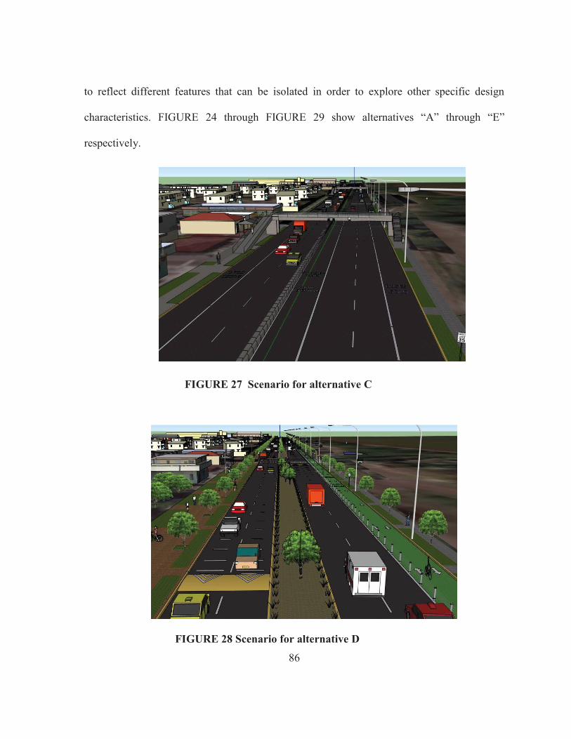
86
to reflect different features that can be isolated in order to explore other specific design
characteristics. FIGURE 24 through FIGURE 29 show alternatives “A” through “E”
respectively.
FIGURE 27 Scenario for alternative C
FIGURE 28 Scenario for alternative D

87
Three of criteria shown in FIGURE 25 were difficult to represent in the visualizations
due to its abstract concept or difficult understanding for lay people. They were self-
sustainability of infrastructure, rapid construction of infrastructure, ecologically friendly
infrastructure. For that reason, a brief description of the contained features was given to
respondents when shown the multimedia presentation. A special care was took it in to
account to ensure the neutrality in the description of features in order to minimize a possible
a bias in respondents’ preference. Nevertheless the description was added, respondents were
still found difficult to identify the design criteria in the visualizations. The development of
the visualizations required approximately 14 weeks, divided as follows: 2 weeks in
preparatory training in Google SketchUp v8, 4 weeks to build the current corridor and
surroundings, which constitute the “Do-Nothing” alternative, and 2 weeks per each
alternative.
FIGURE 29 Scenario for alternative E

88
5.1 Visual preference questionnaire
The third part of the methodology process (see FIGURE 8) included the evaluation of
preferences over the designed alternatives. In order to achieve this objective a dual
instrument was developed: a written questionnaire and a multimedia presentation. The
questionnaire was chosen because, as explained in subtitle 4.1, the simplicity and
accessibility of this method is suitable for the local context. The questionnaire contains
seven questions divided in two parts. The first part asks about the elements, characteristics
or attributes that the respondent likes or dislikes of alternatives “A” through “E”. The second
part of the questionnaire is composed of two questions. The first question asks respondents to
establish a hierarchy of preference with regard to the 5 presented scenarios. The second
question evaluate whether or not the desired characteristics and/or attributes of each visual
were perceived by respondents. This question was presented in the form a matrix where rows
containing specific questions and columns list all the alternatives plus a “none” option. The
matrix possesses eleven rows corresponding to each design criterion (see TABLE 24). The
questionnaire was presented on two separated sheets in order to be divisible. The latter
allows respondents to see their answers from part 1 while answering part 2.
The questionnaire was complemented by an oral and multimedia presentation. The
presentation includes a brief overview of the study and gave the location of the study area.
Afterwards, a slide describing the main visual features of alternative “A” is shown, followed
by a slide with the fly-through animation. At the end of the animation respondents are
requested to fill out part 1 of the written questionnaire as explained above. This part of the
questionnaire was executed by showing to respondents the slide outlining the features

89
presented, and the 3-D fly-through animations of each alternative. The process is repeated
until the 5 alternatives are presented. The presentation then introduces a slide showing the
five alternatives simultaneously and respondents are requested to fill out part 2 of the
questionnaire.
TABLE 24 Matrix of Questions, Questionnaire B (part II)
According to your opinion: Alt A
Alt B
Alt C
Alt D
Alt E
None
Which alternative would generate employment and economic activity in the community?
Which alternative would reduce air and water pollution? Which alternative would reduce the number of traffic accidents?
Which alternative would improve biking and walking? Which alternative does possess ecological friendly Infrastructure?
Which alternative does favor greenery and landscaping? Which alternative does preserve cultural, historic and archeological elements?
Which alternative would be a self – Sustainable financial system?
Which alternative would reduce of vehicle operation cost?
Which alternative would reduce travel time? Which alternative would be constructed quickly?
The questionnaire was developed so as to be filled out by the respondent without
assistance. Nevertheless, an interviewer was available to assist respondents because of the
interaction between the multimedia presentation and questionnaire. The questionnaire took
approximately 30 minutes to be completed.
The targeted people were community leaders and community residents. The sample
chosen sample attempted to reach the people surveyed in the 2nd stage of this study (see

90
chapter 4). However, the number of people sampled was smaller due to the process
requirements.
In the initial approach consecutive meeting in the community center were planned.
Oral and written invitations distributed to residents and posted in local business. The first
meeting was set up on Thursday May 23rd. However, the attendance was very poor and only
members of the community board were present. Additionally, the participation in local
community leaders meeting was planned. The meeting is periodically organized by a non-
profit organization denominated “Fundación 2010”. Nevertheless, the meeting was not
scheduled by the time of the research field work. For that reason, a different approach was
taken. The sampling technique adopted is denominated “at convenience” and consisted in
interviews held at respondent’s house and public open areas. Respondents were informed
about their rights, such as confidentiality. The multimedia presentation was shown to
respondents using a personal computer (PC). A total of 28 questionnaires were filled out in
both the meetings and personal interviews. This process took place during the months of
July, August and September on 2013. During this process a member of the community board
collaborate. Besides the respondents of the community of “Dulces Labios”, a comparison
group was selected. This group was composed of six peer graduate students, and seventeen
high school students attending a transportation summer camp held at the University of Puerto
Rico. The sampling was also selected at author’s convenience. The process took place during
in July for the high school students and September for the peer graduate students. A copy of
the questionnaire template can be located in the Appendix 7.2.
91
5.2 Analysis of Preferences The data was summarized in tables and analyzed based on the frequencies of the responses.
Each categorical level in the hierarchy corresponds to a number from 1 to 5. The resulting set
of numbers was assumed to be continuous in order to be analyzed quantitatively. Then basic
statistics can be calculated and compared among the groups. The distributions of the
preference values were summarized using boxplots in order to analyze the differences in the
values assigned to each alternative. Boxplots give a simple graphical idea of the central
tendency and variability of each subset of data. Each boxplot reflects the interquartile values
of 75% with upper box line, median with middle line, and 25% with the bottom line. It also
shows the upper and lower whisker lines. Each line extends to the relative maximum value
and relative minimum value within 1.5 times the height of the box (Interquartile range). The
outliers are also show in the form of asterisks (*). They represent the values that are beyond
the upper or lower whisker line. Finally, the mean is also represented by a combined cross-
circular symbol.
FIGURE 30 shows the distribution of the assigned values for each level of the
alternatives hierarchy for the “Dulces Labios” group. The number of responses per each
alternative is 28. The most preferred scenario was the Alternative “E” with a mean value of
1.5. A total of 75% of respondents assigned a value of 1 in the hierarchy, 10% of them
assigned the value of 2, and less that 15% assigned a value of 3,4, or 5. The less preferred
scenario corresponds to the Alternative “A” with a mean value of 4.35. More than 85% of
respondents assigned the last two places in the hierarchy, only a 14% assigned the values of 2
or 3. None of the respondents assigned the number 1.

92
Alternatives B and C have a similar mean value; however the quartiles indicate that the alt B
as most preferred by a least 50% of the respondents. With regard to the Alternative D, the
preference values were consistently located between 2 and 3, with a mean of 2.2.
Alt-EAlt-DAlt-CAlt-BAlt-A
5
4
3
2
1
Ran
king
val
ues
N= 28
FIGURE 30 Boxplot of preference values for Alternatives A to E for “Dulces Labios” group (N=28).
Some outliers are present in the Alternative A and E. This could be consequence of miss
interpretations of the directions given in the question. Some people tended to assign the
values in the inverse order that was indicated. The frequency of values for each alternative is
shown in the Appendix:. A sample for the Alternative E is shown in FIGURE 31.
The same graphical data analysis was performed for the comparison group ( FIGURE
32). The less preferred scenario was also the Alternative A. More than 80% of respondents
placed it in the last level of the hierarchy (value of 5); however, a most preferred alternative
was not completely defined. Moreover, the dispersion among the assigned values was

93
Alt-EAlt-DAlt-CAlt-BAlt-A
5
4
3
2
1
Ran
king
N=23
54321
20
15
10
5
0
Values of preference for Alternative E
Freq
uenc
y
112
3
21
broader than the “Dulces Labios” group. Although the alternative D was considered the most
preferred scenario by at least 50% of respondents, its mean value is similar to the alternative
B. The latter possesses consistency in the values of 2 and 3 (69%). The alternative E was, in
turn, almost equally distributed among the values of 2, 3, and 4.
FIGURE 32 Boxplot of preference values for Alternatives A to E for the comparison group (N=23).
FIGURE 31 Histogram of values of preference for Alternative E in the “Dulces Labios” group.

94
Alternative C shows a wide variability among the assigned values. 39% of
respondents assigned the value of 5, 21% assigned the value of 4, 17% of them assigned the
value of 1, and 21% assigned 21% assigned the value of 2 or 3.
Despite the explicit graphical difference in the values assigned to each alternative for
each group (FIGURE 30 and FIGURE 32) a statistical test of differences on the medians was
performed. When response variables follow a normal distribution and there exits equal
variances, the common method of “Analysis of Variance” (ANOVA) is used. Nevertheless,
as shown in FIGURE 31 the responses are left-skewed, and the Anderson-Darling normality
test gave a p-Value < 0.005 which means that data is very non-normal. Additionally,
FIGURE 33 shows that the variance varies with the fitted value. For that reason, a simple
ANOVA cannot be applied and non-parametric comparison method was chosen.
4.54.03.53.02.52.01.5
4
3
2
1
0
-1
-2
-3
Fitted Value
Res
idua
l
FIGURE 33 Residuals for alternatives A, B, C, D, and E

95
The method chosen to evaluate the differences in medians among the different
alternatives is called the “Friedman” test. It is equivalent to the one-way ANOVA with
repeated measures, and it is applied for correlated observations (the assigned value to one
alternative is dependent of the values assigned to the others). The dependent variable can be
ordinal or interval. The null hypothesis (H0) is that the treatments effects are zero. The
results are shown in TABLE 25.
TABLE 25 Friedman Test on Preferences for the “Dulces Labios” group
Alternative N Estimated medians
Sum of Ranks
Alt-A 28 4.4 122 Alt-B 28 3.0 91 Alt-C 28 3.4 103 Alt-D 28 2.2 62 Alt-E 28 1.0 42
S = 58.60 DF = 4 P = 0.000 Grand median = 2.800
The analysis was performed using the statistics package Minitab ® version 16.1. TABLE 25
shows the estimated medians for the 5 alternatives. The lower values in the estimated
medians correspond to the most preferred alternatives. Then, alternative E (Alt E), with the
smallest median value, was the most preferred alternative for respondents in the community
of “Dulces Labios”. In the same vein, the median for alternative A correspond to the less
preferred alternative. The gran median is 2.8, and the median for each alternative adds a
effect on this values. Finally, the test statistic (S) had a p-value of 0.001 indicates that the
null hypothesis can be rejected at a levels higher than 0.001.

96
TABLE 26 Kruskal-Wallis Test on Preferences, comparison group
Alternative N Estimated medians
Sum of Ranks
Alt-A 23 4.6 97.5 Alt-B 23 2.6 51.0 Alt-C 23 4.0 81.5 Alt-D 23 1.8 46.0 Alt-E 23 3.0 69.0
S = 31.68 DF = 4 P = 0.000 Grand median = 3.200
Similar to the “Dulces Labios” group there is statistical evidence that at least one alternative
is different from the others (p-value<0.001). Alternative A possesses the furthest media in
one extreme and alternative D in the other.
The “Mann-Whitney U Test” test was used to test the difference in the median of
preference for each alternative in between the respondents in the community of “Dulces
Labios”, and the respondents in the comparison group. The null hypothesis is that there is no
difference in the median for a given alternative “i” (i= A,B,C,D,E) between the two groups
group. This test was used to evaluate whether or not the obtained preferences in the
visualizations for a given alternative are dependent on the respondents group. The
assumptions for this test are similar to the “Kruskal-Wallis Test”. It releases the need for
normality and equally of variances; however, it is still assumed that the response values
similar continuous distributions and they are independent.
TABLE 27 shows the comparison of the medians of preferences for Alternative E
between respondents in the community of “Dulces Labios” and the comparison group. The
null hypothesis is that both medians are equal. The two-tailed test gave a p-values<0.001,
meaning that the null hypothesis Ho: MDulces-Labios = MComparison-group can be rejected.

97
Consequently the medians of preference for alternative E in both groups are statistically
different. The same test was performed for alternatives A, B, C and D. The results are shown
in appendix 7.8.
TABLE 27 Mann-Whitney Test for preferences in Alternative E between the “Dulces Labios” and comparison group
Test Statistics
Alternative E Mann-Whitney U 181.500 Wilcoxon W 587.500 Z -3.312 Asymp. Sig. (2-tailed) .001
TABLE 28 Kruskal-Wallis Test for preferences in Alternative E between the “Dulces Labios” and comparison group
SOURCE N Median Ave
Rank Z
Dulces Labios 28 1 18 -4.25 Comparion 23 3 35.8 4.25
Overall 51 26 H = 18.06 DF = 1 P = 0.000
H = 20.22 DF = 1 P = 0.000 (adjusted for ties)
The test statistic (H) (TABLE 28) had a p-value of 0.001, both adjusted and unadjusted for
ties indicates that the null hypothesis can be rejected at a levels higher than 0.001. Then,
there enough evidence that both median are statistically different.

98
5.3 Criteria design validation The second part of the questionnaire aimed to validate the interpretation of the initial
respondents’ preferences with regard to the design criteria (see FIGURE 24) used in the
visualizations (as embodied in Alternatives A-E). The data collected in the criteria selection
matrix (TABLE 24) was disaggregated per each alternative. A histogram of the frequencies
of criterion selection was selected was generated for each alternative and compared with the
set of criteria shown in FIGURE 25. These graphical representations are shown from
FIGURE 34 through FIGURE 38. In each graphic, the vertical axis gives the complete list of
11 criteria, whereas the rectangle group the specific set of criteria used in the design of the
corresponding alternative. Each bar represents the number of people who that criterion is
benefited by the corresponding alternative. Each respondent was asked 11 questions related
to the design criteria and six answer alternatives are shown, five corresponding to each
alternative and one “none” option. A total of 15 people completed this part of the
questionnaire. (28)

99
FIGURE 34 Histogram of identified criteria versus selected criteria for Alternative E, “Dulces Labios” group
FIGURE 35 Histogram of identified criteria versus selected criteria for Alternative D, “Dulces Labios” group
14 6
10 6
0 1
4 2
4 3
1
0 2 4 6 8 10 12 14
1st Crit2nd Crit3rd Crit4th Crit5th Crit6th Crit7th Crit8th Crit9th Crit
10th Crit11th Crit
0 5
1 4
8 4 4
1 2
3 1
0 2 4 6 8 10 12 14
1st Crit2nd Crit3rd Crit4th Crit5th Crit6th Crit7th Crit8th Crit9th Crit
10th Crit11th Crit

100
FIGURE 36 Histogram of identified criteria versus selected criteria for Alternative C, “Dulces Labios” group
FIGURE 37 Histogram of identified criteria versus selected criteria for Alternative B, “Dulces Labios” group
0 3
0 3
0 0 0
2 1
4 9
0 2 4 6 8 10 12 14
1st Crit2nd Crit3rd Crit4th Crit5th Crit6th Crit7th Crit8th Crit9th Crit
10th Crit11th Crit
0 0
1 0
6 6
2 1
2 3
0
0 2 4 6 8 10 12 14
1st Crit2nd Crit3rd Crit4th Crit5th Crit6th Crit7th Crit8th Crit9th Crit
10th Crit11th Crit

101
FIGURE 38 Histogram of identified criteria versus selected criteria for Alternative A. “Dulces Labios” group For each set of design criteria, an ideal frequency value of 15 was expected in each
alternative. In FIGURE 34, all of the addressed criteria were adequately identified; however,
others criteria such as preservation of cultural elements, Operation cost, and rapid
construction were also present Moreover, less that 50% of respondents identified the 2nd and
3rd criteria. This could be caused by different reasons in the design, e.g., inclusion or
omission of specific features, questionnaire design and spelling, as well as individual
characteristics of respondents, e.g., personal experience. However, because the fuzziness of
responses and many factors that influence people behavior, further research must be
implemented in this area. The same pattern is seen for alternatives D and C (FIGURE 35
FIGURE 36). Although, alternative D was designed considering the 4th to 7th criteria, the
inclusion of greenery and landscaping influenced in the identification of the 2nd criterion
0 0
1 1
0 0 0
1 2
1 3
0 2 4 6 8 10 12 14
1st Crit2nd Crit3rd Crit4th Crit5th Crit6th Crit7th Crit8th Crit9th Crit
10th Crit11th Crit

102
(“Reduction air and water pollution”) as a criteria design. In the case of alternative C, the
four criteria (8th to 11th) were also identified by respondents. Nevertheless, an average of 6
responses was received. Additionally, the 2nd and 4th criteria were also identified. This might
be caused by the inclusion of pedestrian bridges and bus lanes. The alternative B, in turn,
reflects the criteria 5th and 6th with 6 responses out of 15, and criteria 7th and 8th with only 2
and 1 responses out of 15. Both alternatives C and B included the criterion 8th (“Self –
Sustainable financial system”) that was expected to have a very low level of identification
due to the difficulty of represented it graphically. It was identified only by 3 respondents out
of 15. The same phenomenon occurred with criterion 9th (“Reduction of operation cost”). It
was only identified by 1 respondent out of 15.

103
6 CONCLUSIONS, RECOMMENDATIONS AND PERSONAL REFLECTION
6.1 Conclusions
Traditional means of public involvement such as Public Hearings might not reach
important groups of people in the community (e.g. minorities, aging people), and they are
often conducted at a point in time after important decisions by developers have been made.
For that reason a change in the paradigm of public involvement should be promoted.
In this study, early involvement allowed the participation of specific groups such as
community leaders and minorities (e.g. aging people, handicapped) that otherwise would not
have had the chance to express their opinions in traditional Public Hearings. Early
involvement allowed the definition of what is important for interviewed people in the
transportation PDP and tailored the design of alternatives around these preferences.
Additionally, the use of visualizations promoted a different kind of communication in two
ways: first, people easily understood the proposed designs and second, potential designers
can get important public feedback. Thus, the combination of early involvement and
visualizations has great potential to benefit the process of Public Involvement.
Nevertheless, there are some aspects to be considered. First, early involvement requires
logistical resources and trained people to survey people preferences and opinions. Second,
there is no standard in the process of transforming preferences and design criteria into visual
features. Third, the design of the visualizations required expertise in design software and its
elaboration is very time-consuming. Fourth, the quality of the visualizations design of the
alternative might influences the results in people preferences.

104
Approaches such as Sustainable Development, Appropriate Technology and Context
Sensitive Designs, different in detail but similar in goals, aim to generate human well-being
without disturbing the social, economic or environmental systems. The principles that lay
down these approaches have also influenced the transportation sector. Currently the mission
and vision of various Department of Transportations and available literature mention
mobility, accessibility, environmental stewardship, Public Involvement, among others.
However, there exists a gap between what is required in those principles and what it is being
done by current practitioners. This study is an effort to close that gap.
In the literature there are many aspects to be considered in the project development
process for transportation projects. The selection of criteria to be considered in the study
obeys to three main aspects. The first was to cover most of the significant aspect of what is
defined in the reviewed literature for Sustainable Transportation. Second, the number of
pairwise comparisons is limited to the available time when performing the questionnaires.
Questionnaire A brought 11 pairwise comparisons which sometimes tired the respondents,
resulting in loss of attention. Third, the criteria selected should be able to be translated to
visuals. These aspects should be considered when doing similar works.
The results show a gap between the community’s perception of the transportation issues
that affect them and their preferences toward transportation evaluation criteria selected by
respondents. The pairwise comparison resulted in a similar set of preferred criteria. Public
preference might be influenced by media and current socio-economic and political contexts.
The aggregation method that best fits the mathematical requirements and the surveyed public
preferences is the Geometric mean. However, with the exception of the Mode, the other

105
methods also reflected approximately the same upper level of hierarchy of project evaluation
criteria.
The approach of early involvement not only fostered the discussion about design aspect,
but rather it generates a discussion about the objectives and goals of the project development
process, in which each community member expressed his/her particular or opinion. In this
process it is very important that the visualizations reflect the surroundings of the area where
the project is going to be developed at an adequate degree. People have to identify with the
visualization in a way that internalizes the possible benefits and possible negative
consequences of each alternative being communicated. This aspect was addressed by
showing current scenario (“Do-Nothing” alternative) first and subsequently the alternative
designs. As people already know the current configuration, they could understand how the
proposed alternatives will work.
Visualizations were designed aiming to reflect a given set of criteria. Some criteria (e.g.
rapid construction, water and air pollution, vehicle operation cost) were difficult to represent
graphically. An implemented mechanism to verify if the respondents in the community
identified the desired criteria in each alternative showed that most of the desired criteria were
identified. Nevertheless, as shown in FIGURE 34 to FIGURE 38, some sets of criteria were
not fully identified by every respondent.
Sometimes, designers take only one alternative and ask community to choose specific
characteristic (e.g., size, form); by not evaluating the adequacy of this feature against the
community values, the designer limits the universe of solutions. In this study, Questionnaire
A allowed the identification of important values to consider when addressing transportation

106
issues and proposing alternative of solutions. Additionally, the designer has the freedom to
evaluate more than one feature or set of features, and combine them differently in each
alternative that the “sketch” constitutes. New ideas may arise from the discussion around
these sketches. The visualizations allow the assessment of features’ appropriateness in terms
of the community and design values. This may allow designers to grasp a final design that
not only achieve technical goals, but also lead to consensus and social legitimacy within the
community.
For respondents in the community of “Dulces Labios”, the most preferred alternatives
were those that embodied the most preferred criteria (i.e., the highest ranked). In the same
sense, the alternatives designed with the less preferred alternatives were less preferred.
However, the least preferred alternative in both groups of respondents corresponds to the
alternative “Do-Nothing” (Alt A). Interestingly, this scenario corresponds to a recently
constructed 3-lane corridor, with apparently good levels of service. However, this alternative
was scored with the least preference values when compared to the other alternatives in both
the “Dulces Labios” and Comparison group. Additionally, the preferred alternative is built
with criteria that according to the Logistic regression is influenced by socio-economic
characteristics of the community.
Values of consistency ratios (CR) lower than 0.10 were reached by using the Arithmetic
and Geometric mean as shown in Tables 7 and 8. The lowest consistency ratio value
corresponds to the Geometric mean which is consistent with the reviewed literature. On the
other hand, the Harmonic mean gives a CR value equivalent to twice the value of CR for the
Arithmetic mean in both cases. Similarly, the results show that neither the Percentiles nor the

107
Mode are an adequate approach for aggregating the judgment values. Furthermore, the worst
indices were produced by the Mode. The results show a relationship between the number of
judgments and the CR. The higher the number of judgments is, the lower the consistency
ratio.
When analyzing the preferences, both the group of the Community of “Dulces Labios”
and the overall sample do not show variance among the top three preferred criteria. This is
shown in TABLE 13 and TABLE 14. When comparing between the Arithmetic mean and the
Geometric mean, the first and second preferred criteria are interchangeable while the third
remains the same. The subsequent levels of the hierarchy indicate a disparity among the
ranking values. Among the different aggregation methods, there is an inversion of the
hierarchy for some criteria (e.g. criterion [11]). This could be a consequence of one or the
combination of important characteristics; the sensitivity to the values near to zero for the
Geometric mean and the presence of outliers result in such different values when the
individual values are aggregated. Despite the CR values, about 80% of aggregation methods
considered the criteria numbers 4 and 2 to be preferred in the top 3 levels. 50% of the
methods considered the criteria number 11 to be in the top 3 levels. However, the resulting
hierarchy is primarily based on the methods with CR values under 0.10. Based on the
evidence, the best approach would be the Geometric mean.
Regarding transportation issues affecting the quality of life, the people surveyed in the
community of “Dulces Labios” showed concern with traffic congestion (17% of total
responses), fuel cost (17%), and availability of public transportation (11%). The pavement
quality, the pollution caused by vehicles, safety, security, and the provision of bicycle lanes

108
were around 6% of the total number of responses. As a third group, lacking of facilities for
people with disabilities, vehicle operating and acquisition cost, and parking were around 3%.
These results show that the surveyed people are more concerned with aspects of mobility and
economy rather than social, environmental, or economic development aspects. This is
strongly related to the fact that 63% of people use a private motor vehicle as their primarily
mode of transportation. However, when people were asked about the criteria to be used for
the evaluation of transportation infrastructure, the top criteria was related to the provision of
transportation alternatives. These alternatives include bicycle lanes and sidewalks (11% of
the responses), accessibility (10%), pollution (9%), constructability (8%), and economic
development (8%). Moreover, the top three criteria resulting from the AHP hierarchy were
generation of employment and economic activity in the community, reduction of air and
water pollution, and safety improvements of transportation infrastructure and operations.
6.2 Recommendations
Regarding the criteria used, additional criteria, such as the evaluation of construction cost,
should be incorporated in order to cover other important aspects related to Sustainable
Transportation and the community’s development. Moreover, the designer or researcher
should be aware that the values may vary both between communities and within the same
community over the time. These criteria should then be translated into a language that people
in the community can understand.
Investing time in becoming familiar with the community values and activities is
important. Community members need to recognize the developer, planner or researcher as

109
partner rather than only a public server. This requires implementing different strategies such
as successive visits, informal meetings, and talks. An example would be to get involved in
additional community activities held or organized in the community.
Higher levels of public participation remains to be challenging and different strategies to
incorporate more people in the participatory process should be evaluated. Especially under
especial socioeconomic conditions such as those that exhibit “Dulces Labios”.
There are local and supra-local organizations that represent important links to
communities (e.g. the program of especial communities in Puerto Rico). Further research
should take into account the means of communication that these programs/agencies represent.
Additionally, their experiences and strategies can be used.
Regarding to the design of the visualizations, it would be very useful to work on the
elaboration of add-ons, libraries, or complementary software that allows the quick generation
of alternatives is recommended. Furthermore, this could establish the standards for
alternative development, and streamline the elaboration of the visualizations.

110
6.3 Future work
As an outgrowth of this work, several additional efforts can be pursued to further substantiate
the methodology and to increase its impact in the planning process. These include the
following:
It is very common that initiatives state the importance of community well-being as a
component of sustainability. However, very few take it into account in the proposed
methodology or case study. The conflicting positions of the stakeholders are usually
undertaken or considered a minor issue in the process as compared to the benefits of the
chosen alternatives. In that sense, the analysis of the tradeoffs among the different design
criteria should be further investigated, especially when dynamic techniques such as
public meeting, task forces or similar methodologies are used.
The use of the technique presented in this thesis could be extended to generate more
scenarios with different features combinations that could be shown iteratively to the
community and, ultimately, be combined into one final preferred alternative using
different techniques such as Conjoint Analysis. This final conjoint of features could be
used to evaluate more specific characteristics of the design, engineering standards,
specifications, among others.
It was found that people had problems in the assignment of values during the pairwise
comparison because of the relativeness of human judgments. In that sense, an important
aspect to explore for future studies is the fuzziness in the values assigned during the

111
pairwise comparison. Additionally, the aggregation methods that would work best with
fuzziness could be evaluated.
This study was not meant to establish a list of criteria to be used in alternatives generation.
It was intended to explore a methodology to use visualizations made of conjoint features
to reflect community preferences. For that reason, a methodology in the definition and
judgment of the design criteria reflecting the literature and public preferences can be
implemented.
6.4 Personal reflection During the development of this work the most important lesson learned was that
professionals, and especially engineers, should be aware of the role they develop within
society. They might be aware that the actions they perform directly or indirectly impact
social wellbeing. During the development of this study I had the chance to feel that by
working in a community in Puerto Rico, and applying the principles of Appropriate
Technology, I had a chance to contribute directly to the wellbeing of a community. I believe
that this is the essence of what it means to practice engineering in the best sense.
Engineering is not only a discipline of technical expertise, but it is also about using
interdisciplinary knowledge and sensibility of the broader societal impacts.

112
REFERENCES ______________________________________ Agresti, A., 2002. Categorical Data Analysis. John Wiley & Sons. Al-Kodmany, K., 2001. Visualization tools and methods for participatory planning and
design. Journal of Urban Technology 8, 1–37. Amekudzi, A.A., Meyer, M., Ross, C., 2011. Climate change - Sustainability [WWW
Document]. Sustainability Evaluation and Planning Guidance for Transportation Systems. URL http://www.fhwa.dot.gov/environment/climate_change/sustainability/resources_and_publications/guidebook/index.cfm (accessed 5.20.12).
Arnstein, S.R., 1969. A Ladder of Citizen Participation. Boston: American Institute of Planners. 35, 216–224.
Bailey, K., Blandford, B., Grossardt, T., Ripy, J., 2011. Planning, technology, and legitimacy: structured public involvement in integrated transportation and land-use planning in the United States. Environment and Planning B: Planning and Design 38, 447 – 467.
Bailey, K., Grossardt, T., 2006. Addressing the Arnstein gap: improving public confidence in transportation planning and design through structured public involvement (SPI), in: Proceedings of the 11th International GeoMultimedia Symposium. pp. 337–341.
Bailey, K., Grossardt, T., Pride-Wells, M., 2007. Community design of a light rail transit-oriented development using casewise visual evaluation (CAVE). Socio-Economic Planning Sciences 41, 235–254.
Ball, J., 2002. Towards a methodology for mapping “regions for sustainability”using PPGIS. Progress in Planning 58, 81–140.
Black, W.R., 2005. Sustainable Transport: Definitions and Responses, in: Transportation Research Board Conference Proceedings 37. Presented at the Conference on Introducing Sustainability into Surface Transportation Planning.
Board on Sustainable Development, National Research Council, 1999. Our Common Journey: A Transition Toward Sustainability. The National Academies Press, Washington, D.C.
Castro-Sitiriche, M., Papadopoulos, C., Frey, W., Huyke, H., 2012. Sustainable wellbeing education in engineering, in: 2012 IEEE International Symposium on Sustainable Systems and Technology (ISSST). Presented at the 2012 IEEE International Symposium on Sustainable Systems and Technology (ISSST), pp. 1–6.
CEE, 2011. Sustainability [WWW Document]. Center for Environmental Excellence by AASHTO. URL http://environment.transportation.org/
CEE, 2013. Center for Environmental Excellence by AASHTO: Context Sensitive Solutions [WWW Document]. URL http://environment.transportation.org/environmental_issues/context_sens_sol/#bookmarksubWhatisCSS (accessed 9.3.13).
Center for Computational Research, U. at B., 2009. Visualization in Transportation Design and Regional Planning [WWW Document]. Federal Highway Administration and Federal Transit Administration. URL http://fhwa.ccr.buffalo.edu/video/overview/player.html (accessed 2.16.13).

113
CTE, 2007. Results of Joint AASHTO/FHWA Context Sensitive Solutions Strategic Planning Process. Center for Transportation and the Environment, North Carolina State University.
DTOP, 2010a. DTOP - Visión, Misión e Historia [WWW Document]. Department of Transportation and Public Works (DTPW - DTOP). URL http://sashto.dtop.gov.pr/DTOP/vision_mision.htm (accessed 5.20.12).
DTOP, 2010b. Oficina de Recopilación y Análisis de Tránsito : Departamento de Transportación y Obras Públicas [WWW Document]. URL http://www.dtop.gov.pr/carretera/det_content.asp?cn_id=287 (accessed 9.23.13).
Du Pisani, J., 2006. Sustainable Development – Historical roots of the concept. Environmental Sciences 3, 83 – 96.
Edoho, F.M., n.d. APPROPRIATE TECHNOLOGY TRANSFER. Environment Canada, 2008. Canadian Environmental Assessment Agency - Public
Participation Guide [WWW Document]. Government of Canada. URL https://www.ceaa-acee.gc.ca/default.asp?lang=En&n=46425CAF-1&offset=9&toc=show#a1 (accessed 7.17.13).
EPA, 2011. Guide to Sustainable Transportation Performance Measures [WWW Document]. URL http://www.epa.gov/smartgrowth/transpo_performance.htm (accessed 11.1.11).
Falcocchio, J., 2004. Performance Measures for Evaluating Transportation Systems: Stakeholder Perspective. Transportation Research Record 1895, 220–227.
Federal Highway Administration, n.d. [Archived] Q And A - Archive - Public Involvement - Planning - FHWA [WWW Document]. URL http://www.fhwa.dot.gov/planning/public_involvement/archive/q_and_a/ (accessed 7.18.13).
FHWA, 1996. Public Involvement Techniques for Transportation Decision-Making [WWW Document]. Federal Highway Administration | Office of Planning, Environment, & Realty (HEP) | Planning | Public Involvement. URL http://www.fhwa.dot.gov/planning/public_involvement/publications/techniques/chapter00.cfm (accessed 7.17.13).
FHWA, 2005. A CSS support center for the transportation community. [WWW Document]. Welcome to CSS | Context Sensitive Solutions.org. URL http://contextsensitivesolutions.org/ (accessed 3.1.12).
FHWA, 2009. Context Sensitive Solutions Primer [WWW Document]. URL http://www.fhwa.dot.gov/context/css_primer/ (accessed 8.27.13).
FHWA, 2011. Welcome! | Sustainable Highways Self-Evaluation Tool | Federal Highway Administration [WWW Document]. Sustainable Highways Self-Evaluation Tool - INVEST. URL http://www.sustainablehighways.org/ (accessed 6.18.12).
FHWA, 2013. Authorizing Legislation - Public Involvement - Planning [WWW Document]. URL http://www.fhwa.dot.gov/planning/public_involvement/authorizing_legislation/ (accessed 7.19.13).
FHWA, n.d. NEPA and Transportation Decisionmaking - Public Involvement Overview [WWW Document]. Environmental Review Toolkit | NEPA and Project

114
Development. URL http://environment.fhwa.dot.gov/projdev/tdmpubinv2.asp (accessed 7.19.13).
Field, A.P., 2009. Discovering statistics using SPSS. SAGE, London. Figueroa-Medina, A.M., 1999. Analisis y evaluacion de alternativas en el uso de tecnologia
de transporte colectivo para rutas del Tren Urbano (M.S.). University of Puerto Rico, Mayaguez (Puerto Rico), United States -- Puerto Rico.
Forman, E., Peniwati, K., 1998. Aggregating individual judgments and priorities with the analytic hierarchy process. European Journal of Operational Research 108, 165–169.
Frey, W., Papadopoulos, C., Castro-Sitiriche, M., Zevallos, F., Echevarría Silva, D., 2012. On Integrating Appropriate Technology Responsive to Community Capabilities: A Case Study from Haiti, in: ASEE Annual Conference and Exposition. San Antonio, TX.
Grossardt, T., Bailey, K., Brumm, J., 2001. Analytic Minimum Impedance Surface: Geographic Information System-Based Corridor Planning Methodology. Transportation Research Record 1768, 224–232.
Heijungs, R., Huppes, G., Guinée, J.B., 2010. Life cycle assessment and sustainability analysis of products, materials and technologies. Toward a scientific framework for sustainability life cycle analysis. Polymer Degradation and Stability 95, 422–428.
Hixon III, C., 2007. Visualization Issues for Transportation Agencies: Approaches and Challenges. Visualization in Transportation Empowering Innovation TR NEWS 252.
Hixon III, C.L., 2006. NCHRP SYNTHESIS 361: Visualization for Project Development. Transportation Research Board National Research.
Hosmer, D.W., Lemeshow, S., 2000. Applied Logistic Regression, 2nd ed. Wiley-Interscience Publication.
Hughes, R., 2004. Visualization in Transportation: Current Practice and Future Directions. Transportation Research Record: Journal of the Transportation Research Board 1899, 167–174.
ICF International, CH2M Hill, Inc. and Trans Tech, 2009. Integrating Context Sensitive Solutions into Transportation Practice Guide [WWW Document]. URL http://contextsensitivesolutions.org/content/reading/integrating_context_sensitive_s_/resources/Integrating_CSS_into_Transportation_Practice_Guide.pdf/ (accessed 5.16.12).
Insituto de Estadísticas de Puerto Rico, 2003. Inventario de Estadísticas de Puerto Rico [WWW Document]. URL http://www.estadisticas.gobierno.pr/iepr/Estadisticas/InventariodeEstadisticas/tabid/186/ctl/view_detail/mid/775/report_id/c1bcd196-f0d3-4237-a8d6-32d0a52678e7/Default.aspx (accessed 7.2.12).
International Association for Public Participation, 2007. IAP2 Spectrum of of Public Participation [WWW Document]. (c) International Association for Public Participation www.iap2.org. URL http://www.iap2.org/associations/4748/files/IAP2%20Spectrum_vertical.pdf (accessed 7.18.13).

115
International Association of Public Participation, 2006. IAP2’s PUBLIC PARTICIPATION TOOLBOX [WWW Document]. (c) International Association for Public Participation www.iap2.org. URL http://iap2.affiniscape.com/associations/4748/files/06Dec_Toolbox.pdf (accessed 5.16.12).
Ishizaka, A., Labib, A., 2011. Review of the main developments in the analytic hierarchy process. Expert Systems with Applications 38, 14336–14345.
Jeon, C.M., 2010. Incorporating Uncertainty into Transportation Decision Making: Sustainability-Oriented Approach. Transportation Research Record: Journal of the Transportation Research Board 2174, 58–67.
Jeon, C.M., Amekudzi, A.A., 2005. Addressing Sustainability in Transportation Systems: Definitions, Indicators, and Metrics. Journal of Infrastructure Systems 11, 31–50.
Jeon, C.M., Amekudzi, A.A., Guensle, R.L., 2010. Evaluating Plan Alternatives for Transportation System Sustainability: Atlanta Metropolitan Region - International Journal of Sustainable Transportation.
John A. Volpe National Transportation Systems Center, 2007. Visualization Case Studies: A Summary of Three Transportation Applications of Visualization [WWW Document]. GIS in Transportation. URL http://www.gis.fhwa.dot.gov/documents/visual_toc.htm (accessed 7.23.13).
John A. Volpe National Transportation Systems Center, 2009. Applications of 3D Visualization: Peer Exchange Summary Report. FHWA, U.S. DOT, Raleigh, North Carolina.
Litman, T.A., 2007. Developing Indicators for Comprehensive and Sustainable Transport Planning. Transportation Research Record: Journal of the Transportation Research Board 2017, 10–15.
Litman, T.A., 2009. Sustainable Transportation Indicators: A Recommended Research Program For Developing Sustainable Transportation Indicators and Data. Presented at the Transportation Research Board 88th Annual Meeting.
Méndez, L., Piaggio, M., 2007. Desarrollo sustentable en zonas costeras uruguayas desde la dimensión económica. Unidad de Gestión Ecoplata. 36pp.
Montgomery, D.C., Runger, G.C., 2006. Applied Statistics and Probability for Engineers, 4th ed. Wiley.
Moore, K.R., 2012. Context Sensitive Solutions:Federal Perspective of MAP-21. Mori, K., Christodoulou, A., 2010. Review of sustainability indices and indicators: Towards
a new City Sustainability Index (CSI). Environmental Impact Assessment Review. OECD, 1996. CONFERENCE HIGHLIGHTS AND AND OVERVIEW OF ISSUES, in:
CONFERENCE HIGHLIGHTS AND OVERVIEW OF ISSUES. Presented at the TOWARDS SUSTAINABLE TRANSPORTATION, http://www.oecd.org/, Vancouver, British Columbia.
Ohman, K.V.H., 2008. Applying a decision support system tool to the integrated design and operation of a landfill (Ph.D.). University of Calgary (Canada), Canada.
Organisation for Economic Co-operation and Development, 2001. Performance Indicators for the Road Sector: Summary of the Field Tests. OECD Publishing.

116
Oswald, M.R., McNeil, S., 2010. Rating Sustainability: Transportation Investments in Urban Corridors as a Case Study. J. Urban Plng. and Devel. 136, 177.
Parris, T.M., Kates, R.W., 2003. CHARACTERIZING AND MEASURING SUSTAINABLE DEVELOPMENT. Annual Review of Environment and Resources 28, 559–586.
Practical Action, 2012. What is Appropriate Technology? | Practical Answers | Practical Action [WWW Document]. URL http://practicalaction.org/what-is-appropriate-technology (accessed 10.29.13).
Ramani, T.L., Zietsman, J., Potter, J., Reeder, V.S., 2012. A Guidebook for Sustainability Performance Measurement for Transportation Agencies. Presented at the Transportation Research Board 91st Annual Meeting.
Ravana, S.D., Moffat, A., 2009. Score aggregation techniques in retrieval experimentation, in: Proceedings of the Twentieth Australasian Conference on Australasian Database - Volume 92, ADC ’09. Australian Computer Society, Inc., Darlinghurst, Australia, Australia, pp. 57–66.
RITA, 2012. Table 3-5: U.S. Gross Domestic Demand (GDD) Attributed to Transportation-Related Final Demand [WWW Document]. Research and Innovative Technology Administration | Bureau of Transportation Statistics. URL http://www.rita.dot.gov/bts/sites/rita.dot.gov.bts/files/publications/national_transportation_statistics/html/table_03_05.html (accessed 7.16.13).
Saaty, T.L., Vargas, L.G., 2000. Models, Methods, Concepts & Applications of the Analytic Hierarchy Process, 1st ed. Springer.
Sheppard, S.R.J., 2006. Bridging the sustainability gap with landscape visualisation in community visioning hubs. Integrated Assessment Journal 6, 79–108.
Sinha, K.C., Labi, S., 2007. Transportation Decision Making: Principles of Project Evaluation and Programming. Wiley.
Stanley, J., Lucas, K., 2013. Workshop 6: The public agenda: What is working and what is missing. Research in Transportation Economics 39, 294–299.
Tharakan, J., 2008. The Relevance of Appropriate Technology. Presented at the 3rd International Conference on Appropriate Technology, Kigali, Rwanda.
Tharakan, J., 2010. Appropriate Technologies for Water and Sanitation. Presented at the 4th International Conference on Appropriate Technology, Accra, Ghana.
The Boston Foundation, 2000. Boston Indicators Project [WWW Document]. URL http://www.bostonindicators.org/ (accessed 11.3.13).
Toleman, R., Rose, G., 2008. Partnerships for Progress: Toward Sustainable Road Systems. Transportation Research Record: Journal of the Transportation Research Board 2067, 155–163.
United Nations Division for Sustainable Development, 1992. Agenda 21 [WWW Document]. URL http://www.un.org/esa/dsd/agenda21/ (accessed 5.15.12).
WCED, W.C.O.E. and development, 1987. Our Common Future. Oxford University Press, USA.
Willoughby, K.W., 1990. Technology Choice: A Critique of the Appropriate Technology Movement. Westview Press.

117
Winterfeldt, D. von, 2000. Developing Performance Measures for Complex Evaluations: An Introduction and an Application to Upgrading Infrastructure Systems. 2000 32.
World Bank, 2011. Roads & Highways [WWW Document]. URL http://web.worldbank.org/WBSITE/EXTERNAL/TOPICS/EXTTRANSPORT/EXTROADSHIGHWAYS/0,,contentMDK:20472045~pagePK:210058~piPK:210062~theSitePK:338661,00.html (accessed 9.9.11).
Wu, W.H., Chiang, C.T., Lin, C.T., 2008. Comparing the aggregation methods in the analytic hierarchy process when uniform distribution. WSEAS Transactions on Business and Economics 5, 74–80.

118
7 APPENDIXES
7.1 Questionnaire A


119
7.2 Questionnaire B


120
7.3 Letter of Inform Consent


121
7.4 Letter of authorization from the Institutional Review Board committee (IRB) (CPSHI by its acronym in Spanish)


122
7.5 Appendix: Histograms of preference values
5432
18
16
14
12
10
8
6
4
2
0
Alt-A
Freq
uenc
y
17
7
1
3
Histogram of Alt-A
Figure 39 Histogram of preference values for Alternative A in the “Dulces Labios” group
Figure 40 Histogram of preference values for Alternative B in the “Dulces Labios” group
54321
12
10
8
6
4
2
0
Alt-B
Freq
uenc
y
2
12
67
1
Histogram of Alt-B

123
5432
14
12
10
8
6
4
2
0
Alt-C
Freq
uenc
y
76
14
1
Histogram of Alt-C
Figure 41 Histogram of preference values for Alternative C in the “Dulces
Labios” group
54321
14
12
10
8
6
4
2
0
Alt-D
Freq
uenc
y
12
5
14
6
Histogram of Alt-D
Figure 42 Histogram of preference values for Alternative D in the “Dulces Labios” group

124
54321
20
15
10
5
0
Alt-E
Freq
uenc
y
112
3
21Histogram of Alt-E
Figure 43 Histogram of preference values for Alternative E in the “Dulces Labios” group

125
7.6 Logistic Regression (cont.)
The logistic model was originally used for epidemiologic research (Hosmer and
Lemeshow, 2000). Currently, it is widely used in many fields such as finance, engineering,
health policy and linguistics, among others. For instance, some credit-scoring applications
use logistic regression to model the probability that a subject is credit worthy (Agresti, 2002).
In this thesis, the logistic regression is applied to evaluate the relationship among socio-
demographic characteristics of the people surveyed and the odds of selecting or not a given
design criteria as important for the design of a transportation project in the Community of
“Dulces Labios”.
The distinction between linear models and logistic models is reflected in the choice of
the parametric model and the assumptions. However, once this difference is accounted for,
they follow the same general principles for their analysis (Hosmer and Lemeshow, 2000).
The probability of selecting or not a criterion is assumed that follows the discrete Bernoulli
distribution. It follows then that it can only take the exclusive values of 0 or 1. The
probability distribution is shown in TABLE 29; the probability that the outcome will be 1 is
represented by , and the probability that outcome will be 0 is represented by .
TABLE 29 Probability of the outcome that follows a Bernoulli distribution
Outcome(Yi) Probability 1 P(Yi =1)= 0 P(Yi =0)= 1 -
The expected value of the response variable E (Yi|xi) is defined as:
(8)

126
The expected value for the response variable and the probability that the response
takes the value of 1 are the same. Empirical evidence shows that when the outcome variable
is dichotomous, the shape of the response will follow a S-shaped curve that gradually
approaches 0 and 1 (Hosmer and Lemeshow, 2000; Montgomery and Runger, 2006).
FIGURE 44 shows an example of the probability of failure versus temperature of a given
process.
The S-shape function is called the logistic response function. For binary response variable Y
and an explanatory variable “x”, let The
specific form of the logistic regression model is:
(9)
FIGURE 44 Probability of failure versus temperature of a given process (Data taken from Montgomery & Runger (2006)).

127
The logit transformation corresponds to a linearization of the logistic regression model and is
expressed in equation 10. This will be called simply the logit or the log odds.
x10=(x)-1
(x)ln=g(x) (10)
The estimation of the parameter is performed using the maximum likelihood method.
To apply the method, a likelihood function is first constructed. It reflects the probability of
the observed data as a function of the unknown parameter. Estimates ( ) are chosen in such
a way that the function is maximized. If the dichotomous outcome is coded as 0 and 1, the
pairs ( xi,yi) whose “yi” is equal to 1 will contribute π(xi) to the likelihood function. In the
same vein, the pairs whose “yi” is equal to 0 will contribute (1-π(xi)) to the likelihood
function. Because each pair is assumed independent, the total contribution of all pairs could
be interpreted as shown in (11):
x-1]x[=)l( ii y-1i
n
1=i
yi (11)
If If
corresponds to the natural logarithm of . is also denominated as “Log
likelihood” in statistical software packages. The estimate of β that maximizes this equation
will be used.
(12)

128
This expression is partially differentiated with respect to β0 and β1 and equaled to zero in
order to find the β that maximizes the expression. The results are the “maximum likelihood
estimates of β and denoted as and respectively. This is easily estimated with
statistic software (e.g. Minitab ®)
The evaluation of the significance of the coefficients is performed by comparing the
observed values to the predicted values with and without the variable in question. This
comparison does not constitute a “goodness-of-fit” test, but rather is a relative comparison
among the models that include different variables. The comparison is based on the log
likelihood function for both the fitted and saturated model. The latter relationship is
called the likelihood ratio. The same expression is used to calculate the deviance [D]
(equivalent to the residual sum of squares in linear regression, SSE)
model saturated theof likelihoodmodel fitted theof likelihood-2Ln=D
When the outcome has only two possible values (0, 1), the likelihood of the saturated
model is 1. In order to assess the significance of an independent variable, the value of D for
both the model with and without the variable are compared
variable the withlikelihoodariable without vLikelihood-2Ln=G (13)
For the case of multiple logistic regressions, the procedure to fit the model is the same as the
univariate model. The logit is shown in (14).
pp3322110 x…x +x +x +=g(x) (14)

129
The logistic regression model is:
Given “n” independent observations (xi, yi), where i = 1,2,3… n. Each sample
observation follows the Bernoulli distribution, thus the likelihood function is:
(15)
The method requires obtaining the vector of coefficients β’= ( β0, β1, β2, β3 … βp).
These coefficients are also estimated using the likelihood function. There are “p+1”
likelihood equations obtained by differentiating the log likelihood function with respect to
the “p+1” coefficients. The univariate case has only one independent variable, then p+1 =
1+1= 2. Let be the solutions to these equations, and then the fitted values are denoted
by . According to the theory of maximum likelihood, the estimators are obtained from
the second partial derivatives of the likelihood function (with respect to , j=1,2,…p). The
results of these derivatives are presented in the form of a matrix that allows the calculation of
the variance and covariance of the estimated coefficients. The jth diagonal element of the
matrix corresponds to the variance of . In the same sense, correspond to the
covariance between and . Once a particular model is fit, its significance can be assessed.
The first step is to check the significance of the variables in the model. The test is based on
the G statistic given in equation (13).

130
Finally, different kind of independent variables can be included at the same time,
including intervals, ordinals, and nominal variables. There are cases where numbers are
wrongly included in the model as intervals. In the case variables are merely identifiers, a
collection of design variables (dummy or indicator variables) must be used (Agresti, 2002). If
there are “c” classes the number of dummy variables will be “c-1”. For instance, the model to
be developed considers three level of education (EDU), two dummy variables will be needed
(EDU1, EDU2). Intervals variables can be treated as ordinals if the data number is small. In
the same vain, ordinals variables could be assigned with a numeric value and be used as
intervals variables. Each category has a difference in magnitude than the other and a
underlying continuous variable is assumed (Agresti, 2002).
.

131
7.7 Logistic regression output tables
TABLE A 1 Logistic regression output for criteria [1]: Reduction of travel time Odds 90% CI Predictor Coef SE Coef Z P Ratio Lower Upper Constant -1.63304 0.833306 -1.96 0.05 AGE -0.007561 0.012813 -0.59 0.555 0.99 0.97 1.01 GEN 0.208385 0.436661 0.48 0.633 1.23 0.6 2.53 CATV -0.497858 0.514738 -0.97 0.333 0.61 0.26 1.42 RTVR -0.20165 0.652308 -0.31 0.757 0.82 0.28 2.39 PDP1 -0.277697 0.601607 -0.46 0.644 0.76 0.28 2.04 EISD 0.486139 0.552407 0.88 0.379 1.63 0.66 4.03 PPUH -0.366338 0.61791 -0.59 0.553 0.69 0.25 1.92 EDU2 0.703226 0.462369 1.52 0.128 2.02 0.94 4.32 PRIM1
1 0.439711 0.711322 0.62 0.536 1.55 0.48 5 2 0.0485756 0.607855 0.08 0.936 1.05 0.39 2.85
Tests for terms with more than 1 degree of freedom Term Chi-Square DF P PRIM1 0.388300 2 0.824 Log-Likelihood = -72.704 Test that all slopes are zero: G = 8.683, DF = 10, P-Value = 0.562 Goodness-of-Fit Tests Method Χ2 DF P Pearson 185.512 174 0.261 Deviance 145.408 174 0.944 Hosmer-
Lemeshow 8.117 8 0.422
TABLE A 2 Logistic regression output for criteria [2]: Generation of employment and economic activity in the community
Odds 90% CI Predictor Coef SE Coef Z P Ratio Lower Upper Constant -0.55649 0.638878 -0.87 0.384 AGE 0.001495 0.009831 0.15 0.879 1 0.99 1.02 GEN 0.5784 0.348252 1.66 0.097 1.78 1.01 3.16 CATV 1.54866 0.419948 3.69 0 4.71 2.36 9.39 RTVR 0.359816 0.49686 0.72 0.469 1.43 0.63 3.24 PDP1 0.629951 0.488553 1.29 0.197 1.88 0.84 4.19

132
EISD -1.36025 0.432547 -3.14 0.002 0.26 0.13 0.52 PPUH 0.013792 0.453725 0.03 0.976 1.01 0.48 2.14 EDU2 -0.01912 0.367448 -0.05 0.958 0.98 0.54 1.8 PRIM1
1 -1.01531 0.518587 -1.96 0.05 0.36 0.15 0.85 2 -0.09904 0.47742 -0.21 0.836 0.91 0.41 1.99
Tests for terms with more than 1 degree of freedom Term Chi-Square DF P PRIM1 3.94023 2 0.139 Log-Likelihood = -106.774 Test that all slopes are zero: G = 40.656, DF = 10, P-Value = 0.000 Goodness-of-Fit Tests Method Χ2 DF P Pearson 187.752 174 0.225 Deviance 210.776 174 0.030 Hosmer-
Lemeshow 5.710 8 0.680
Coefficientsa Model Collinearity
Statistics Tolerance VIF
1 AGE 0.753 1.328 GEN 0.942 1.062 CATV 0.665 1.505 RTVR 0.751 1.332 PRIM1 0.845 1.184 PDP1 0.801 1.248 EISD 0.749 1.335 PPUH 0.835 1.198 EDU2 0.828 1.208
a. Dependent Variable: Criteria [2]

133
TABLE A 3 Logistic regression output for criteria [3]: Rapid construction of the infrastructure
Odds 90% CI Predictor Coef SE Coef Z P Ratio Lower Upper Constant -2.25333 0.943702 -2.39 0.017 AGE 0.024866 0.013175 1.89 0.059 1.03 1 1.05 GEN -0.65842 0.509478 -1.29 0.196 0.52 0.22 1.2 CATV -0.66632 0.620079 -1.07 0.283 0.51 0.19 1.42 RTVR -1.29024 0.85016 -1.52 0.129 0.28 0.07 1.11 PDP1 -0.04626 0.642782 -0.07 0.943 0.95 0.33 2.75 EISD 0.690035 0.573032 1.2 0.229 1.99 0.78 5.12 PPUH -1.41484 0.866489 -1.63 0.103 0.24 0.06 1.01 EDU2 0.055369 0.570197 0.1 0.923 1.06 0.41 2.7 PRIM1
1 0.16263 0.698103 0.23 0.816 1.18 0.37 3.71 2 -0.09337 0.700892 -0.13 0.894 0.91 0.29 2.88
Tests for terms with more than 1 degree of freedom Term Chi-Square DF P PRIM1 0.102302 2 0.950 Log-Likelihood = -61.676 Test that all slopes are zero: G = 11.864, DF = 10, P-Value = 0.294 Goodness-of-Fit Tests Method Χ2 DF P Pearson 178.685 174 0.388 Deviance 123.352 174 0.999 Hosmer-
Lemeshow 5.112 8 0.746
TABLE A 4 Logistic regression output for criteria [4]: Reduction of air and water pollution
Odds 90% CI Predictor Coef SE Coef Z P Ratio Lower Upper Constant 0.438113 0.631441 0.69 0.488 AGE -0.02823 0.009685 -2.91 0.004 0.97 0.96 0.99 GEN -0.25003 0.325534 -0.77 0.442 0.78 0.46 1.33 CATV 1.43249 0.414691 3.45 0.001 4.19 2.12 8.29 RTVR -0.17981 0.489494 -0.37 0.713 0.84 0.37 1.87 PDP1 -0.59886 0.468445 -1.28 0.201 0.55 0.25 1.19

134
EISD 0.460224 0.384877 1.2 0.232 1.58 0.84 2.98 PPUH 0.717806 0.436613 1.64 0.1 2.05 1 4.2 EDU2 0.037534 0.349909 0.11 0.915 1.04 0.58 1.85 PRIM1
1 -0.5752 0.516728 -1.11 0.266 0.56 0.24 1.32 2 -0.21289 0.457366 -0.47 0.642 0.81 0.38 1.72
Tests for terms with more than 1 degree of freedom Term Chi-Square DF P PRIM1 1.26578 2 0.531 Log-Likelihood = -115.754 Test that all slopes are zero: G = 21.483, DF = 10, P-Value = 0.018 Goodness-of-Fit Tests Method Χ2 DF P Pearson 185.262 174 0.265 Deviance 231.508 174 0.002 Hosmer-
Lemeshow 10.37 8 0.24
TABLE A 5 Logistic regression output for criteria [5]: Including greenery and landscaping
Odds 90% CI Predictor Coef SE Coef Z P Ratio Lower Upper Constant -0.95805 0.656461 -1.46 0.144 AGE -0.01106 0.009733 -1.14 0.256 0.99 0.97 1 GEN 0.546387 0.340007 1.61 0.108 1.73 0.99 3.02 CATV 0.198424 0.413928 0.48 0.632 1.22 0.62 2.41 RTVR 0.274355 0.498447 0.55 0.582 1.32 0.58 2.99 PDP1 0.272089 0.498858 0.55 0.585 1.31 0.58 2.98 EISD -0.23979 0.398368 -0.6 0.547 0.79 0.41 1.52 PPUH 0.35415 0.444582 0.8 0.426 1.42 0.69 2.96 EDU2 -0.07886 0.360993 -0.22 0.827 0.92 0.51 1.67 PRIM1
1 -0.34567 0.559703 -0.62 0.537 0.71 0.28 1.78 2 -0.1079 0.468905 -0.23 0.818 0.9 0.42 1.94
Tests for terms with more than 1 degree of freedom Term Chi-
Square DF P
PRIM1 0.389183 2 0.823

135
Log-Likelihood = -108.760 Test that all slopes are zero: G = 6.588, DF = 10, P-Value = 0.764 Goodness-of-Fit Tests Method Χ2 DF P Pearson 185.256 174 0.266 Deviance 214.748 174 0.019 Hosmer-
Lemeshow 10.908 8 0.207
TABLE A 6 Logistic regression output for criteria[6]: Ecologically-friendly Infrastructure. (Recycled materials, Solar energy, etc.)
Odds 90% CI Predictor Coef SE Coef Z P Ratio Lower Upper Constant -1.14543 0.679821 -1.68 0.092 AGE -0.003532 0.009916 -0.36 0.722 1 0.98 1.01 GEN 0.239803 0.349689 0.69 0.493 1.27 0.72 2.26 CATV -0.215636 0.424711 -0.51 0.612 0.81 0.4 1.62 RTVR -0.089026 0.518234 -0.17 0.864 0.91 0.39 2.15 PDP1 0.564502 0.519084 1.09 0.277 1.76 0.75 4.13 EISD -0.348032 0.408713 -0.85 0.394 0.71 0.36 1.38 PPUH -0.11249 0.473389 -0.24 0.812 0.89 0.41 1.95 EDU2 0.287055 0.372513 0.77 0.441 1.33 0.72 2.46 PRIM1
1 -0.151842 0.568182 -0.27 0.789 0.86 0.34 2.19 2 -0.103596 0.485883 -0.21 0.831 0.9 0.41 2
Tests for terms with more than 1 degree of freedom Term Chi-Square DF P PRIM1 0.0950762 2 0.954 Log-Likelihood = -104.504 Test that all slopes are zero: G = 3.413, DF = 10, P-Value = 0.970 Goodness-of-Fit Tests Method Χ2 DF P Pearson 184.236 174 0.283 Deviance 206.234 174 0.048 Hosmer-
Lemeshow 5.317 8 0.723

136
TABLE A 7 Logistic regression output for criteria [7]: Infrastructure for bicycle/pedestrian movement
Odds 90% CI Predictor Coef SE Coef Z P Ratio Lower Upper Constant 0.0922252 0.593563 0.16 0.877 AGE 0.0026631 0.008584 0.31 0.756 1 0.99 1.02 GEN 0.475732 0.309764 1.54 0.125 1.61 0.97 2.68 CATV -0.075889 0.376813 -0.2 0.84 0.93 0.5 1.72 RTVR -0.302766 0.461431 -0.66 0.512 0.74 0.35 1.58 PDP1 -0.559048 0.436841 -1.28 0.201 0.57 0.28 1.17 EISD 0.178724 0.360105 0.5 0.62 1.2 0.66 2.16 PPUH -0.418196 0.421466 -0.99 0.321 0.66 0.33 1.32 EDU2 0.155952 0.334503 0.47 0.641 1.17 0.67 2.03 PRIM1
1 0.008905 0.47801 0.02 0.985 1.01 0.46 2.21 2 0.0479864 0.430525 0.11 0.911 1.05 0.52 2.13
Tests for terms with more than 1 degree of freedom Term Chi-Square DF P PRIM1 0.0125439 2 0.994 Log-Likelihood = -125.402 Test that all slopes are zero: G = 6.510, DF = 10, P-Value = 0.771 Goodness-of-Fit Tests Method Χ2 DF P Pearson 183.892 174 0.289 Deviance 248.031 174 0 Hosmer-
Lemeshow 13.545 8 0.094
TABLE A 8 Logistic regression output for criteria [8]: Reduction of vehicle operatiing cost
Odds 90% CI Predictor Coef SE Coef Z P Ratio Lower Upper Constant -2.39125 0.854728 -2.8 0.005 AGE -0.002484 0.012132 -0.2 0.838 1 0.98 1.02 GEN 0.57369 0.426648 1.34 0.179 1.77 0.88 3.58 CATV 0.237695 0.511044 0.47 0.642 1.27 0.55 2.94 RTVR 0.183663 0.631196 0.29 0.771 1.2 0.43 3.39 PDP1 0.597517 0.644128 0.93 0.354 1.82 0.63 5.24

137
EISD -0.578405 0.486383 -1.19 0.234 0.56 0.25 1.25 PPUH -0.176224 0.589482 -0.3 0.765 0.84 0.32 2.21 EDU2 0.745219 0.445692 1.67 0.095 2.11 1.01 4.39 PRIM1
1 -0.892158 0.84413 -1.06 0.291 0.41 0.1 1.64 2 -0.089882 0.584023 -0.15 0.878 0.91 0.35 2.39
Tests for terms with more than 1 degree of freedom Term Chi-Square DF P PRIM1 1.12057 2 0.571 Log-Likelihood = -77.754 Test that all slopes are zero: G = 8.842, DF = 10, P-Value = 0.547
Goodness-of-Fit Tests Method Χ2 DF P Pearson 179.984 174 0.362 Deviance 152.736 174 0.876 Hosmer-
Lemeshow 10.651 8 0.222
TABLE A 9 Logistic regression output for criteria [9]: Self – Sustainable financial system
Odds 90% CI Predictor Coef SE Coef Z P Ratio Lower Upper Constant -1.65847 0.766803 -2.16 0.031 AGE 0.0011201 0.011449 0.1 0.922 1 0.98 1.02 GEN 0.535272 0.405836 1.32 0.187 1.71 0.88 3.33 CATV -0.282544 0.476159 -0.59 0.553 0.75 0.34 1.65 RTVR -0.664171 0.614993 -1.08 0.28 0.51 0.19 1.42 PDP1 -0.037296 0.582982 -0.06 0.949 0.96 0.37 2.51 EISD -0.017811 0.497932 -0.04 0.971 0.98 0.43 2.23 PPUH 0.600619 0.512861 1.17 0.242 1.82 0.78 4.24 EDU2 0.80644 0.427758 1.89 0.059 2.24 1.11 4.53 PRIM1
1 -0.313013 0.668928 -0.47 0.64 0.73 0.24 2.2 2 -0.725559 0.626687 -1.16 0.247 0.48 0.17 1.36
Tests for terms with more than 1 degree of freedom Term Chi-Square DF P PRIM1 1.37609 2 0.503 Log-Likelihood = -82.921 Test that all slopes are zero: G = 11.084, DF = 10, P-Value = 0.351

138
Goodness-of-Fit Tests Method Χ2 DF P Pearson 176.239 174 0.438 Deviance 163.069 174 0.713 Hosmer-
Lemeshow 7.955 8 0.438
TABLE A 10 Logistic regression output for criteria [10]: Preservation of cultural, historic and archeological elements
Odds 90% CI Predictor Coef SE Coef Z P Ratio Lower Upper Constant -2.2611 0.814549 -2.78 0.006 AGE 0.0032208 0.010359 0.31 0.756 1 0.99 1.02 GEN -0.09119 0.369045 -0.25 0.805 0.91 0.5 1.68 CATV 0.0328575 0.464364 0.07 0.944 1.03 0.48 2.22 RTVR -0.56511 0.582377 -0.97 0.332 0.57 0.22 1.48 PDP1 1.26606 0.617394 2.05 0.04 3.55 1.28 9.79 EISD 0.30952 0.426531 0.73 0.468 1.36 0.68 2.75 PPUH -0.857375 0.530672 -1.62 0.106 0.42 0.18 1.02 EDU2 -0.306897 0.40983 -0.75 0.454 0.74 0.37 1.44 PRIM1
1 0.498214 0.535096 0.93 0.352 1.65 0.68 3.97 2 0.692179 0.481851 1.44 0.151 2 0.9 4.41
Tests for terms with more than 1 degree of freedom Term Chi-Square DF P PRIM1 2.34863 2 0.309 Log-Likelihood = -95.883 Test that all slopes are zero: G = 14.062, DF = 10, P-Value = 0.170 Goodness-of-Fit Tests Method Χ2 DF P Pearson 188.53 174 0.214 Deviance 188.993 174 0.207 Hosmer-
Lemeshow 6.766 8 0.562
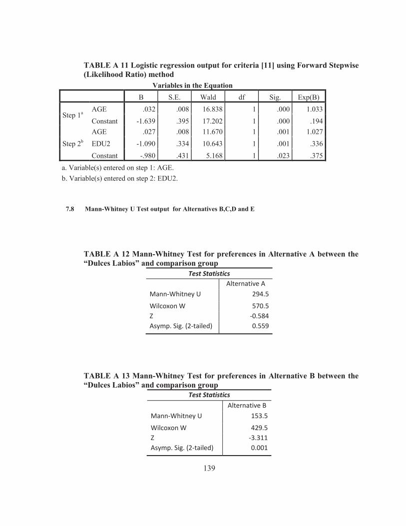
139
TABLE A 11 Logistic regression output for criteria [11] using Forward Stepwise (Likelihood Ratio) method
Variables in the Equation B S.E. Wald df Sig. Exp(B)
Step 1a AGE .032 .008 16.838 1 .000 1.033 Constant -1.639 .395 17.202 1 .000 .194
Step 2b AGE .027 .008 11.670 1 .001 1.027 EDU2 -1.090 .334 10.643 1 .001 .336 Constant -.980 .431 5.168 1 .023 .375
a. Variable(s) entered on step 1: AGE. b. Variable(s) entered on step 2: EDU2.
7.8 Mann-Whitney U Test output for Alternatives B,C,D and E
TABLE A 12 Mann-Whitney Test for preferences in Alternative A between the “Dulces Labios” and comparison group
Test Statistics Alternative A Mann-Whitney U 294.5
Wilcoxon W 570.5 Z -0.584 Asymp. Sig. (2-tailed) 0.559
TABLE A 13 Mann-Whitney Test for preferences in Alternative B between the “Dulces Labios” and comparison group
Test Statistics Alternative B Mann-Whitney U 153.5
Wilcoxon W 429.5 Z -3.311 Asymp. Sig. (2-tailed) 0.001

140
TABLE A 14 Mann-Whitney Test for preferences in Alternative C between the “Dulces Labios” and comparison group
Test Statistics Alternative C
Mann-Whitney U 316
Wilcoxon W 722 Z -0.118 Asymp. Sig. (2-tailed) 0.906
TABLE A 15 Mann-Whitney Test for preferences in Alternative D between the “Dulces Labios” and comparison group
Test Statistics Alternative D Mann-Whitney U 275
Wilcoxon W 551 Z -0.93 Asymp. Sig. (2-tailed) 0.352