sustainability and economics of aviation industry

University of Bergamo

Department of Management, Information and Production

Engineering

University of Pavia

Department of Economics and Management

Ph.D. in Economics and Management of Technology XXX cycle

Doctoral Dissertation

Sustainability and Economics of Aviation Industry

Supervisor: Prof. Gianmaria MARTINI Candidate: Pak Lam LO ___________________________________________________________________________

October 2017

Acknowledgement Thank God for the adventure, the lessons, the failures and the supports prepared at the right time in my life, eventually the peaceful mind. Thank the academics community for the excellent environment for me to learn and grow.

Prof. Gianmaria Martini, who encourages and cultivates me by providing valuable opportunities in all dimensions, deserves the appreciation from the deepest of my heart.

Prof. Davide Scotti, who is always helpful in researches and academic tasks, is the first one whom I seek help from when I am in trouble.

Prof. Martin Dresner’s warm welcome from the University of Maryland expands my horizons. ATRS and ATARD scholars’ demonstration of interesting researches in different approaches. Colleagues and staff members of the Universities contributing to an entertaining and comfortable student life.

Thank my family for their love. Thank my friends for their patience.

Content 1. Introduction and summary

2. The impact of technology progress on aviation noise and emissions

2.1. Introduction

2.2. Literature review

2.3. Empirical strategy

2.3.1. Emission and noise in aviation

2.3.2. Econometric model

2.4. Data

2.5. Result

2.5.1. Result of the analysis at the flight level

2.5.1.1. Local air pollutants

2.5.1.2. Global pollutants

2.5.1.3. Noise

2.5.2. Result of the analysis at the passenger level

2.5.2.1. Local air pollutants

2.5.2.2. Global pollutants

2.5.2.3. Noise

2.5.3. Discussion

2.6. Conclusion

2.7. Reference

3. The determinants of CO2 emissions of air transport passenger traffic: An analysis applied

to Lombardy (Italy)�

3.1. Introduction


3.3. Empirical Strategy

3.3.1. Measuring of aviation CO2 emission


3.4. Data

3.5. Result

3.6. Conclusion

3.7. Reference

4. Econometric Approach to Reveal Determinants of Air Cargo Volume of European

Countries

4.1. Introduction

4.2. Air Cargo Industry in Europe


4.4. Empirical Strategy

4.4.1. Data mining


4.5. Data

4.6. Result

4.7. Conclusion

4.8. Reference

Introduction and Summary Aviation draws people’s attention, not only because it is a dream of human race to fly or the association to vacations, but its role in our modern economies. It is, first of all, an incredible investment, such as airports1, aircrafts, lands, control systems…etc. There are great business opportunities as well as risks2. Moreover, the operation of airports3, airlines or aircraft manufacturing4 generate tremendous incomes and jobs, often vital to cities heavily relay on these business. Furthermore, politic issues, such as regulations, agreements, ownerships and business decisions in company level, are shaping the market. Last but not least, enhanced by aviation, the connectivity and attractiveness of city induce economic benefit in tourism, business and so on, are very seductive to governors hoping to exploit its economic potential. However, just like any aspect of economics, there are externalities, which is not always captured nor considered by decision makers. Externality is always the first question I ask. To quantify and internalize them will enhance market efficiency and the fairness of society. Furthermore, the trend, abnormality or unobserved factors are crucial in this uncertain world if we want to estimate the future. Focusing on econometrics, i.e. applying statistical tools on economic data to spot estimators and to set models; reference points for discussion or decision could be provided while arousing the awareness of less-acknowledged matters by including them in the models. Three papers are presented in this report. First of all, as the fastest growing transport mode, aviation sustainability and environmental costs are generally concerned. We tried to address the noise and emission of the global aircraft fleet and to argue the current technology progress is not vigorous enough, while examining the trade off of these externalities. We find a statistically significant impact of incremental technical progress on all environmental externalities. Substantial innovation is found to have positive effect on per-passenger externalities. These results point to the need for incentives in aviation technical progress. Secondly, the blooming of passenger traffic, particularly contributed by low cost carrier (LCC) across Europe is changing the landscape of aviation market: revitalizing airports, exploiting regulations and inducing policies. By observing the carbon dioxide footprint of flights departing from four airports in Lombardy region, we reveal determinants having direct impact on CO2 emissions in two dimensions: total emission and per available seat kilometer (emission efficiency). Also we show distinguished characteristics of LCC and try to capture the impact of air traffic policies of government and airlines. Last but not least, we are interested in a less studied area of aviation industry – air cargo activities. In the era of new economy, characterized by just in time manufacturing and express e-commerce, GDP as the classic indicator of air cargo should be verified since GDP is weighting more on service industries nowadays but less on air-cargo-related manufacturing

1 Construction cost of an airport can be up to billions, and sometimes involve land formation. Some example from “Airport construction mid-year review”, CAPA 2015. 2 Delays of an airport opening can induce over-budget and harm business. The case of Berlin airport highlighted by “The farcical saga of Berlin's new airport”, The Telegraph 2017. 3Memphis, whose economy is driven by trucking and transportation, is the “America’s Distribution Hub” hosting FedEx headquarter.4“Fears for 4,000 British jobs as Bombardier hit with 219pc US tariffs in subsidy dispute”, The Telegraph 2017. The dispute of USA (Boeing) and Canadian Bombardier may affect jobs in Belfast, Northern Ireland, where part of the aircraft is produced.

industries. This is an attempt to estimate air cargo activities, which is an important component of the air transport industry and a strong driver of aviation development other than air passenger movement. We found that a country’s income level, online purchase activity and air cargo connectivity are all positive determinants of its air cargo level.

The impact of technology progress on aviation noise andemissions

Mattia Grampella a,⇑, Pak Lam Lo b, Gianmaria Martini c, Davide Scotti caDepartment of Earth and Environmental Science, University of Milan Bicocca, 20126 Milano, ItalybDepartment of Economics, University of Pavia, 27100 Pavia, ItalycDepartment of Management, Information and Production Engineering, University of Bergamo, 24044 Dalmine (BG), Italy

a r t i c l e i n f o

Article history:Available online 12 June 2017

Keywords:Technical progressEnvironmental externalitiesAircraft/engine combinations

a b s t r a c t

This paper investigates the effects of incremental and substantial innovations on aviationemissions and noise levels among aircraft/engine combinations belonging to the BoeingB737 and the Airbus A320 families. We find a statistically significant impact of incrementaltechnical progress on all environmental externalities both at the flight level and the pas-senger level. Although substantial innovation is found to have a limited impact at the flightlevel, a noteworthy positive effect exists on per-passenger externalities. These results pointto the need for incentives in aviation technical progress in order to neutralize future neg-ative environmental effects due to the expected traffic growth.

! 2017 Elsevier Ltd. All rights reserved.

1. Introduction

Aviation continues to be a booming industry, with an annual growth rate that has often surpassed 4.6% in the past tenyears,1 which is 3.5% greater, on average, than advanced economies’ GDP growth.2 Such growth, boosted by the extension ofderegulation as well as an increasing level of competition brought about by the entrance of low-cost carriers (LCC), is expectedto continue for the next years. Although competition and development are beneficial since they have brought about lower faresand greater mobility to the air transportation industry, both the public and policymakers are increasingly concerned about theindustry’s overall impact on the environment.

At the global level, the aviation industry accounts for 3.5% of global greenhouse gases (Lee et al., 2009), with a predictedincrease of 15% by 2050 (IPCC, 1999); however, at the local level, emissions and noise nuisance are the biggest concernsbecause such factors may harm areas outside the airport (the human population, animals, plants, water, soil, etc.). Heavyhealth impacts are related to both emissions (respiratory and brain diseases, as well as cancers) and noise nuisance (hearingimpairment, hypertension, ischemic heart disease, annoyance, sleep disturbance, stress).

As the public agrees that environmental externalities should be internalized into the cost of the industry, several environ-mental standards and corresponding platforms have been introduced at global, regional, and local levels. On a global level,the Kyoto Protocol (signed in 1997) aims at fighting global warming by reducing greenhouse gas concentrations in the atmo-sphere. On a regional level, the European Union emission-trading scheme (started in 2005) was extended to airlines in 2012.

http://dx.doi.org/10.1016/j.tra.2017.05.0220965-8564/! 2017 Elsevier Ltd. All rights reserved.

⇑ Corresponding author.E-mail address: [email protected] (M. Grampella).

1 According to Statista, annual growth (2006–2014) in global air traffic passenger demand has always been greater than 4.6%, except in 2008 and 2009,resulting in an average growth rate of 4.8% (Statista, 2015).

2 According to the IMF database, the GDP growth from 2006 to 2014 of advanced economies was +1.3% on average.

Transportation Research Part A 103 (2017) 525–540

Contents lists available at ScienceDirect

Transportation Research Part A

journal homepage: www.elsevier .com/locate / t ra

On a local level, many European cities have applied curfew and emission and/or noise surcharges to incentivize operators toreduce pollution.

As indicated by Chèze et al. (2011a), emissions in air transportation could be reduced by energy efficiency gains in (1) airtraffic management (ATM), (2) improvements in existing aircraft (incremental innovation), and (3) production of new air-craft (substantial innovation). Different from driver (1), factors (2), and (3) are both related to technical progress. Moreover,Leylekian et al. (2014) show that both incremental and substantive innovation can also contribute to noise reduction.

Despite the acknowledged importance of innovation in reducing aviation externalities, little is known about the ways thatadvances in new technology are shaping the air transportation industry.3

This paper is an attempt to fill this gap. To this end, we build a data set composed of 270 different aircraft/engine com-binations that belong to the B737 and A320 families and investigate the influence of technical progress (innovation) on (i)noise, (ii) local pollutants, and (iii) global pollutants. Further, we look for the existence of a trade-off between noise and localpollutants, as suggested by previous studies (e.g., Phleps and Hornung, 2013). Last, we investigate the relationship betweenthe size of newly designed aircraft and the per-passenger environmental impact. To the best of our knowledge, the currentstudy is one of the first attempts to measure the influence of technical progress in air transportation through an econometricapproach. We have not found many systematic statements in the literature on the effects of technological progress at boththe flight and the passenger levels (a rare example is Swan, 2010).4 Despite this lack of evidence, other than enhancing fuelefficiency, the tendency of building bigger aircraft is also magnifying the environmental impact of a single flight. We pose thequestions: What is such an impact per single passenger transported? Would the marginal environmental cost of a single pas-senger decrease even if the increasing marginal cost of the single flight is taken into account?

The structure of the paper is as follows. Section 2 summarizes the literature contributions on the relationship betweentechnological progress and the environmental impact of air transportation. Section 3 presents the aviation externalities con-sidered in the analysis, the sources of technical progress, and the econometric model. Section 4 describes the data set used inthis study and the corresponding data mining procedures. Section 5 presents the empirical results. Section 6 concludes thepaper and highlights some possible policy implications.

2. Literature review

Previous literature on the environmental impact of air transportation has mainly focused on computing the amount ofemissions and noise produced by airports or particular aircraft types and converting such amounts into a monetary damage.

Schipper (2004) studies the impact of aircraft operations on air pollution and noise in a small group of European airports.He focuses on some routes and calculates, by aggregating aircraft and routes factors, the annual monetary damages. A similarapproach is followed by Lu and Morrell (2006), but applied only at Heathrow, Gatwick, Stansted, Schipol, and Maastricht air-ports. Several contributions carry out a quantification of monetary damages of emissions and noise. Morrell and Lu (2007)calculate the environmental costs of hub-to-hub versus hub-bypass networks applying the methodology presented in Lu andMorrell (2006) to a data set of eight large airports on different continents. Lu (2009) calculates the impact on air passengerdemand of the introduction of emission charges in airfares. Givoni and Rietveld (2010) compare the environmental costs ofusing two different aircraft types (the narrow-body A320 and the wide-body B747) on two high-demand routes (London-Amsterdam and Tokyo-Sapporo). Lu (2011) calculates the environmental costs at the Taiwan Taoyuan International Airportfollowing the approach of Lu and Morrell (2006). Miyoshi and Mason (2009) propose an aircraft-specific calculator for CO2

emissions applied to U.K. domestic routes, intra-Europe routes serving the U.K., and North Atlantic routes.To the best of our knowledge, only a few contributions have estimated the effect of innovation on environmental impacts.

These studies mainly focus on fuel consumption and CO2. Macintosh andWallace (2009) provide an estimate of CO2 aviationemissions from 2005 to 2025 using the following algorithm: Et ¼ RTKt " EIt , in which Et is the emission of CO2 in year t, RTKt

is the projected revenue tonne kilometers, and EIt is the emission intensity in aviation in year t. They assume a reduction inemissions equal to 1.9% per year, in line with the IATA target. After deriving calibrations and running different scenarios, theauthors show that innovation is unlikely to offset the increase in CO2 emissions. Chèze et al. (2011a) also measure innovationin terms of higher fuel efficiency, which leads to lower CO2 emissions. They provide a historical trend of technical progress inaviation, both in terms of fuel consumption and CO2 emissions, and show that the amount of energy burnt by an aircraft(measured in MJoule) per available seat kilometer (ASK) has improved by a factor of 3.5 between 1958 (when the Comet4 aircraft model was issued) and 2011 (the introductory year of the A350-300). Moreover, using an algorithm similar to thatof Macintosh and Wallace (2009), they compute that innovation has improved energy efficiency by 2.88% per year in theperiod 1983–2006. In order to obtain this result they assume an approximately 3% annual reduction in tonnes of jet fuelby available tonne kilometer, but consider in their evaluation both technical progress and improvements in ATM. Chèzeet al. (2011b) extend this approach and analyze the impact of energy efficiency on aviation CO2 emissions by showing thatnew aircraft are not necessarily more efficient than older ones. For instance, carbon intensity, measured as grams of CO2 perrevenue passenger kilometer (RPK), is higher for the new aircraft A380 (equal to 101.86 g CO2/RPK), than for the B777-300

3 Aircraft and engine manufacturers claim that newer aircraft burn less fuel, take off and land in shorter times, make less noise, and fly faster. Airportmanaging companies guarantee that noise levels are under control through introducing monetary incentives (i.e., noise surcharges), thus encouraging airlinesto use younger aircraft.

4 Swan (2010) reports that large airplanes make 2–3 times the noise per seat as small airplanes.

526 M. Grampella et al. / Transportation Research Part A 103 (2017) 525–540

(launched in 1997, with 92.84 g CO2/RPK). Furthermore, Chèze et al. (2013) suggest that, if current trends in technologicalprogress in aviation continue, the projected annual increase in the amount of CO2 generated is equal to +0.1% at the worldlevel, and that the current innovation process (in fuel efficiency) is not outweighing the carbon emissions of the growing airtraffic. Brugnoli et al. (2015) examine the various forces influencing the development of environmentally beneficial technicalchanges in commercial aircraft and find CO2 reductions of about 1.34% a year due to endogenous technical progress.

All previous contributions estimate that innovation effects on fuel consumption and CO2 emissions is approximately#1.3%/#3% yearly, however, this amount is based on algorithms (with the exception of Brugnoli et al. (2015)). This impliesthat ad hoc assumptions about future scenarios are required (e.g., future advances in technologies) and that any kind of sta-tistical inference on the provided coefficients is not allowed. Moreover, the literature contributions do not include all of theaviation externalities, since they focus mainly on CO2 and completely ignore the noise component.

We see the need for a study that investigates the effect of the aviation industry’s incremental and substantial technologyprogress on both pollutant emissions and noise. Incremental innovation is given by the annual improvement in environmen-tal performance—i.e., how much a younger technology improves—while substantial innovation refers to the introduction ofnew aircraft models.

Additionally, Phleps and Hornung (2013) highlight the possible trade-off between emissions and noise in air transporta-tion. They analyze the impact on airline costs through two innovations: the geared turbofan and the rotating open rotor tech-nologies. A comparison is made with the status quo technology, given by the latest models of the B737 and A320 families.They equate three possible scenarios: a ‘‘baseline” scenario that is similar to the current situation, a ‘‘green and growth” sce-nario that balances the production of externalities and the growth of aviation, and a ‘‘rapid aviation growth” scenario payingvery little attention to environmental effects. They show that the open rotor aircraft may yield up to 9% higher fuel efficiencycompared to a geared turbofan technology (and better than the status quo), but that these gains may be completely offset dueto the implementation of higher noise standards (e.g., tighter ICAO future Annex chapters), pointing out that the technicalprogress limiting fuel consumption (and in turn emissions) is not complementary with noise annoyance reductions.

We will encompass these algorithms/scenario-based analyses by comparing the magnitude with indications of the effectsof technical progress on emissions and noise levels from our estimated econometric model. Different indications wouldimply the presence of the Phleps and Hornung (2013) trade-off.

3. The empirical strategy

Our empirical investigation explores the following issues. First, we identify the different aviation externalities—that is,what externalities to investigate and how to quantify them. Second, we design an econometric model estimating the impactof technical progress on such externalities, after having controlled for different factors that may introduce, if omitted, somedistortions in the estimates. Hence, in this section we first describe the types of externalities included in the analysis, andthen present the specifications of our econometric model.

3.1. Emissions and noise in aviation

To evaluate the aviation externalities, we focus on the amount of local and global pollutants emitted, as well as the noisegenerated by different aircraft-engine combinations. This means that our reference point is purely a single flight and not anairport with its total volume of operations. In this way, we can identify the effect of technology progress on a particular flight,which could be regarded as a benchmark for regulation standards.

As shown extensively in Grampella et al. (2017), aviation emissions can be divided into landing and takeoff (LTO) emis-sions,5 affecting mainly the local pollutant concentration, and global emissions, which affect climate change.

Dings et al. (2003) point out that LTO emissions are HC (hydrocarbon), CO (carbon monoxide), NOx (nitrogen oxides), SO2

(sulfur dioxide), and PM10 (particular matters), while global emissions are CO2 (carbon dioxide), H2O (moisture), contrailsand NOx. Dings et al. (2003) extensively discuss the relevance of these different emissions and highlight the following issues.First, global emissions are mostly produced during the aircraft cruise; hence, the total amount of emissions depends uponthe stage length. This finding implies that some assumptions are needed to quantify the amount of global emissions. We con-sider seven stage lengths: 125 nautical miles (nm), 250 nm, 500 nm, 750 nm, 1,000 nm, 1,500 nm, and 2,000 nm. Second, ascontrails only affect 10% of the cruise, we exclude them from the analysis. Third, while CO2 and H2O emissions are related tofuel consumption, NOx global emissions are instead not related to fuel consumption, but depend upon combustion temper-ature, which increases with engine power settings. We follow Sutkus et al. (2001), who provide factors of 3.155 kg CO2/kgfuel, 1.237 kg H2O/kg fuel, as well as emission indices of NOx depending on the aircraft/engine combination and the cruisealtitude (we use a 9–13 km altitude). Fuel consumption for the seven different stage lengths is taken from the CORINAIRdatabase.6

5 Local emissions are mainly related to airport operations—i.e., aircrafts’ different phases composing the LTO-cycle: taxing-in and taxing-out, take-off,climbing (up to 3000 ft) and final approach-landing.

6 CORINAIR does not differentiate engines but only aircraft models. Hence the amount of CO2 and H2O produced during cruise is based on aircraft model only,independent of the engine installed. See the EMEP/CORINAIR Emission Inventory Guidebook for more information.

M. Grampella et al. / Transportation Research Part A 103 (2017) 525–540 527

After first considering each pollutant alone, we then multiply the total amount of each substance by the monetary valueof its cost of damage and obtain aggregate measures of both local pollution and global pollution. Such a cost quantifies, inmonetary terms, the negative health effects of a pollutant. A comprehensive survey on the different approaches and evidenceon pollutants’ monetary damages is provided by Dings et al. (2003), a paper that represents a benchmark for many studies onaviation emissions (e.g., Givoni and Rietveld, 2010; Martini et al., 2013a, 2013b; Scotti et al., 2014; Grampella et al., 2017).The benchmarking costs of damage of pollutants considered in this contribution are as follows: € 4/kg HC, € 9/kg NOx, € 6/kgSO2, and € 150/kg PM10

7 for local emissions, and €4/kg NOx, € 0.03/kg CO2, and € 0.0083/kg H2O for global emissions.The treatment of noise levels is more complex than that of emissions. On the one hand, noise can be measured linearly as

a modification of the sound pressure. On the other hand, noise creates annoyance at the local level—the units of measure arerespectively micro Pascal (lPa) and decibels (dB).8 Human beings can perceive variations in sound pressure produced by anoise source if the sound occurs between 20 lPa (corresponding to a status quo level in which no noise is perceived) and100 Pa (corresponding to the noise produced by an aircraft at maximum thrust power of its engines). The ratio of these twoextreme is greater than 1 million. Although the human ear responds to stimulus produced by noise in a nonlinear way, it doesfollow a logarithmic scale. We consider both dimensions, as they are useful in different interpretations. According to ICAO cer-tification data, noise is evaluated at three points: lateral, flyover, and take-off (climbing) during the LTO operations.

The literature regarding the cost of damage caused by noise is more limited than that regarding air pollution. Some con-tributions (e.g. Schipper, 2004; Lu and Morrell, 2006) have presented estimates based on specific case studies; however,these measures are airport-specific and cannot be easily generalized.9 As a result, we choose to analyze separately the impactof innovation on noise from that on emissions. As previously mentioned, we would also like to determine if any trade-off existsbetween noise and air pollution.

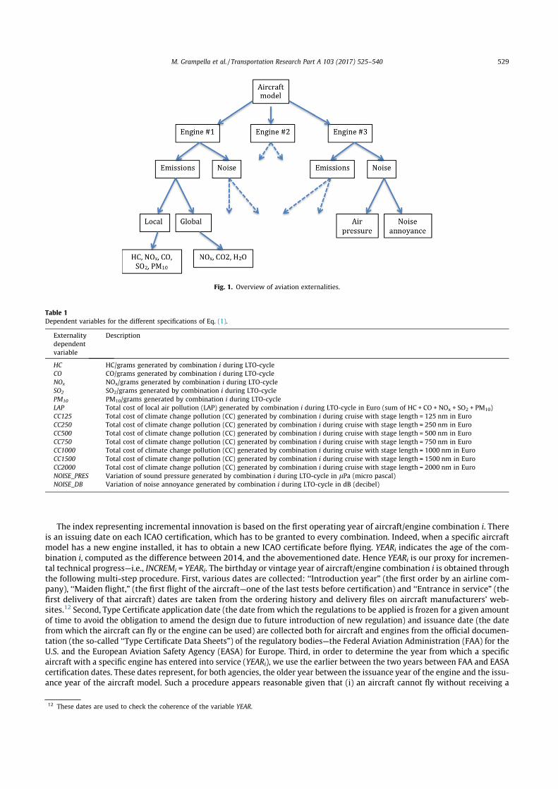
Employing the ICAO certification system, we obtain emissions and noise for each aircraft-engine combination, as shownin Fig. 1, which also provides an overview of the externalities investigated in the analysis.

3.2. The econometric model

Our aim is to estimate the effect of technical progress on the amount of local air pollution, greenhouse gas (GHG) emis-sions, and noise produced by aviation. Moreover, we are also interested in untangling the effect of technical progressbetween per-flight externalities and per-passenger externalities. The former considers the amount of externalities generatedby a single flight, while the latter considers the costs and benefits of individual mobility, as shown by Swan (2010). Hence,we have two measurement units of externalities as a dependent variable: (i) per-flight and (ii) per-seat.10

In the analysis of noise externalities, we consider the magnitude and the sign of technical progress in terms of the soundpressure variation, as well as the noise-level variation as perceived by human ears (see Brüel and Kjær, 2000; Passchier-Vermeer and Passchier, 2000). The former is linear, and thus the estimated coefficient describes the impact of technologyprogress on noise levels under the same (linear) unit, while the latter is logarithmic and hence the estimated coefficient dis-plays the impact on decibels. Thus, an annual reduction of 1 dB obtained through technical progress would not imply a unitdecrease in noise annoyance.11

Echoing to Chèze et al. (2011a, 2011b), we study both incremental and substantial innovation. Incremental technical pro-gress is given by the annual variation in the aircraft/engine combinations’ age, embedding general technical progress in avi-ation technology. Substantial innovation is given by the introduction of a new aircraft model.

As we are interested in estimating the annual percentage variation in aviation externalities in the presence of a unitincrease in the incremental innovation index and the introduction of a new aircraft model, we estimate a log-linear model.The basic econometric model is therefore given by the following equation:

log EXTERi ¼ aþ b1 " INCREMi þ b2 " SUBSTANi þXL

l¼1

cl " CONTRli þ !i; ð1Þ

where EXTERi is the amount of externality produced by the aircraft/engine combination i (see Table 1 for the list of variablesand corresponding measurement units), INCREMi is the index of incremental innovation in combination i, SUBSTANi is theindex of substantial innovation in i, CONTRli is a set of L control variables, while !i is the error term.

7 The estimated health effects of CO produced during the LTO cycle are negligible and therefore not considered in the aggregate measure of local air pollutioncosts.

8 Decibels (dB), a logarithmic scale is the universal measurement of perceived noise annoyance.9 An exception is Grampella et al. (2017), in which Schipper’s (2004) two measures of monetary damages related to noise annoyance are adopted to quantify

the social cost of the noise generated by aircraft during the LTO cycle.10 We consider the seats available on a typical aircraft/engine configuration. This means that we do not consider passenger load factors, which depend uponairlines’ strategies (e.g., airfares, promotions, etc.). Hence, we do not focus on actual emissions in operating conditions (that will be a function of load factors,which in turn, influences thrust power), but on emissions in certified conditions, which are homogenous for all combinations (in terms of thrust power) andtherefore feasible in comparing different models.11 For instance, two noise sources of 50 dB that reaches the same person give rise to a noise annoyance equal to 53 dB—that is, a 3-dB increase represents adouble level of noise annoyance.


The index representing incremental innovation is based on the first operating year of aircraft/engine combination i. Thereis an issuing date on each ICAO certification, which has to be granted to every combination. Indeed, when a specific aircraftmodel has a new engine installed, it has to obtain a new ICAO certificate before flying. YEARi indicates the age of the com-bination i, computed as the difference between 2014, and the abovementioned date. Hence YEARi is our proxy for incremen-tal technical progress—i.e., INCREMi = YEARi. The birthday or vintage year of aircraft/engine combination i is obtained throughthe following multi-step procedure. First, various dates are collected: ‘‘Introduction year” (the first order by an airline com-pany), ‘‘Maiden flight,” (the first flight of the aircraft—one of the last tests before certification) and ‘‘Entrance in service” (thefirst delivery of that aircraft) dates are taken from the ordering history and delivery files on aircraft manufacturers’ web-sites.12 Second, Type Certificate application date (the date from which the regulations to be applied is frozen for a given amountof time to avoid the obligation to amend the design due to future introduction of new regulation) and issuance date (the datefrom which the aircraft can fly or the engine can be used) are collected both for aircraft and engines from the official documen-tation (the so-called ‘‘Type Certificate Data Sheets”) of the regulatory bodies—the Federal Aviation Administration (FAA) for theU.S. and the European Aviation Safety Agency (EASA) for Europe. Third, in order to determine the year from which a specificaircraft with a specific engine has entered into service (YEARi), we use the earlier between the two years between FAA and EASAcertification dates. These dates represent, for both agencies, the older year between the issuance year of the engine and the issu-ance year of the aircraft model. Such a procedure appears reasonable given that (i) an aircraft cannot fly without receiving a

Fig. 1. Overview of aviation externalities.

Table 1Dependent variables for the different specifications of Eq. (1).

Externalitydependentvariable

Description

HC HC/grams generated by combination i during LTO-cycleCO CO/grams generated by combination i during LTO-cycleNOx NOx/grams generated by combination i during LTO-cycleSO2 SO2/grams generated by combination i during LTO-cyclePM10 PM10/grams generated by combination i during LTO-cycleLAP Total cost of local air pollution (LAP) generated by combination i during LTO-cycle in Euro (sum of HC + CO + NOx + SO2 + PM10)CC125 Total cost of climate change pollution (CC) generated by combination i during cruise with stage length = 125 nm in EuroCC250 Total cost of climate change pollution (CC) generated by combination i during cruise with stage length = 250 nm in EuroCC500 Total cost of climate change pollution (CC) generated by combination i during cruise with stage length = 500 nm in EuroCC750 Total cost of climate change pollution (CC) generated by combination i during cruise with stage length = 750 nm in EuroCC1000 Total cost of climate change pollution (CC) generated by combination i during cruise with stage length = 1000 nm in EuroCC1500 Total cost of climate change pollution (CC) generated by combination i during cruise with stage length = 1500 nm in EuroCC2000 Total cost of climate change pollution (CC) generated by combination i during cruise with stage length = 2000 nm in EuroNOISE_PRES Variation of sound pressure generated by combination i during LTO-cycle in lPa (micro pascal)NOISE_DB Variation of noise annoyance generated by combination i during LTO-cycle in dB (decibel)

12 These dates are used to check the coherence of the variable YEAR.


certification for both the engine and model, and (ii) as soon as one of the two agencies issues the necessary certificates, theaircraft-engine combination is allowed to fly.13 As confirmation, notice that (i) no aircraft in the data set exhibit an entry intoservice date antecedent to YEARi; and (ii) for each aircraft model, at least one observation has YEARi corresponding to the firstdelivery date.

Substantial innovation is given by the introduction of a new aircraft model, which is represented by a dummy variablethat is equal to 1 for combination i. Hence the substantial innovation variable is given by a set of K – 1 dummy variables(K is the total number aircraft models included in the analysis), and MODki representing combination i—i.e., b2 " SUBSTANi

becomesPK#1

k¼1 bki "MODki.The set of control variables is given by combination i’s size, expressed in maximum take-off weight, MTOWi, and two

dummy variables identifying two specific engine brands—i.e., CFMi and IAEi. The former is equal to 1 if the engine manufac-turer is CFM International, while the latter is equal to 1 if the engine is produced by IAE (International Aero Engines). Hence, theengine manufacturer baseline case is Pratt & Whitney, given that B737s and A320s have installed engines designed only byCFM, IAE, or Pratt & Whitney. The resulting econometric model is as follows:

log EXTERi ¼ aþ b1 " YEARi þXK#1

k¼1

bki "MODki þ c1 "MTOWi þ c2 " CFMi þ c3 " IAEi þ !i: ð2Þ

Eq. (2) is estimated by OLS. Notice that normal error distribution and constant error variance have been tested. In the major-ity of cases, errors are normally distributed, but with non-constant variance.14 To avoid problems of biased standard errors, inthe case of heteroskedasticity, we estimate robust regressions.15

Eq. (2) is estimated under different specifications given that different externalities act as the dependent variable. A list ofsuch variables with their respective short descriptions is shown in Table 1.16 Note that a single pollutant is identified by itschemical abbreviation (such as HC for hydrocarbon and CO for carbon monoxide), while local air pollution (LAP) represents theaggregate cost of damage produced by the joint effect of all the local pollutants generated by each aircraft/engine combination iduring the LTO cycle. An added ‘‘s” as a final letter (see Section 5) indicates the per-seat amount (e.g., HCs and LAPs indicaterespectively the per-seat amount of HC and LAP).17

4. Data

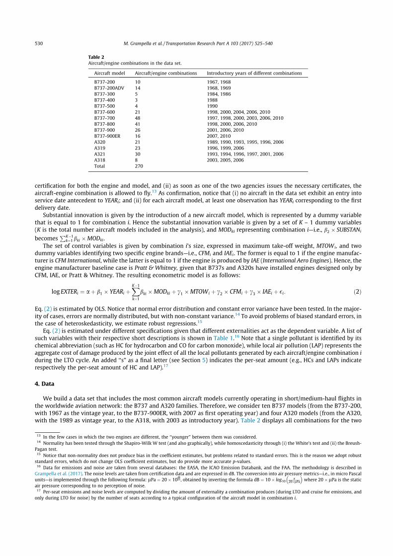
We build a data set that includes the most common aircraft models currently operating in short/medium-haul flights inthe worldwide aviation network: the B737 and A320 families. Therefore, we consider ten B737 models (from the B737-200,with 1967 as the vintage year, to the B737-900ER, with 2007 as first operating year) and four A320 models (from the A320,with the 1989 as vintage year, to the A318, with 2003 as introductory year). Table 2 displays all combinations for the two

Table 2Aircraft/engine combinations in the data set.

Aircraft model Aircraft/engine combinations Introductory years of different combinations

B737-200 10 1967, 1968B737-200ADV 14 1968, 1969B737-300 5 1984, 1986B737-400 3 1988B737-500 4 1990B737-600 21 1998, 2000, 2004, 2006, 2010B737-700 48 1997, 1998, 2000, 2003, 2006, 2010B737-800 41 1998, 2000, 2006, 2010B737-900 26 2001, 2006, 2010B737-900ER 16 2007, 2010A320 21 1989, 1990, 1993, 1995, 1996, 2006A319 23 1996, 1999, 2006A321 30 1993, 1994, 1996, 1997, 2001, 2006A318 8 2003, 2005, 2006Total 270

13 In the few cases in which the two engines are different, the ‘‘younger” between them was considered.14 Normality has been tested through the Shapiro-Wilk W test (and also graphically), while homoscedasticity through (i) the White’s test and (ii) the Breush-Pagan test.15 Notice that non-normality does not produce bias in the coefficient estimates, but problems related to standard errors. This is the reason we adopt robuststandard errors, which do not change OLS coefficient estimates, but do provide more accurate p-values.16 Data for emissions and noise are taken from several databases: the EASA, the ICAO Emission Databank, and the FAA. The methodology is described inGrampella et al. (2017). The noise levels are taken from certification data and are expressed in dB. The conversion into air pressure metrics—i.e., in micro Pascalunits—is implemented through the following formula: lPa ¼ 20" 10

dB20 , obtained by inverting the formula dB ¼ 10" log10 x

20"lPa

! "where 20 " lPa is the static

air pressure corresponding to no perception of noise.17 Per-seat emissions and noise levels are computed by dividing the amount of externality a combination produces (during LTO and cruise for emissions, andonly during LTO for noise) by the number of seats according to a typical configuration of the aircraft model in combination i.


families, which consists of 270 models out of 1460 in the current operating commercial fleet (i.e., about 20% of all aircraft/engine combinations flying today). However, the B737 and A320 families represent a much higher percentage of operatingflights since the vast majority of airlines largely operate these aircraft models, especially low cost carriers (LCCs) (e.g., Rya-nair only operates B737s and EasyJet A320s).18

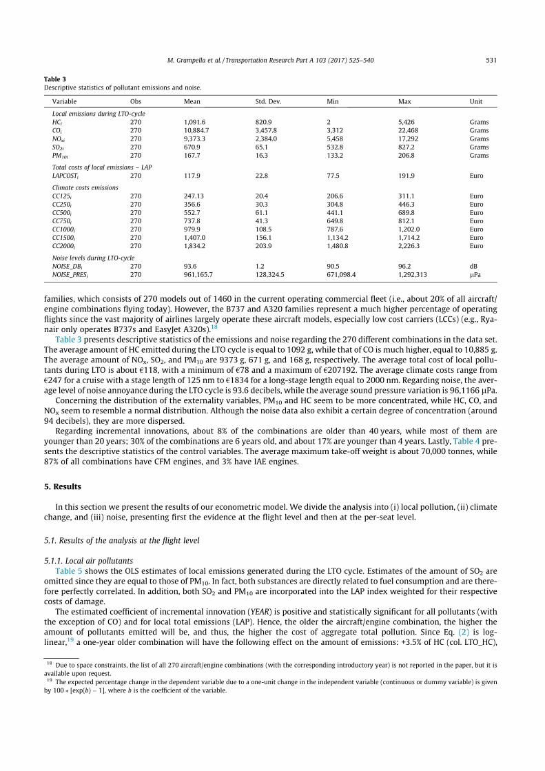
Table 3 presents descriptive statistics of the emissions and noise regarding the 270 different combinations in the data set.The average amount of HC emitted during the LTO cycle is equal to 1092 g, while that of CO is much higher, equal to 10,885 g.The average amount of NOx, SO2, and PM10 are 9373 g, 671 g, and 168 g, respectively. The average total cost of local pollu-tants during LTO is about €118, with a minimum of €78 and a maximum of €207192. The average climate costs range from€247 for a cruise with a stage length of 125 nm to €1834 for a long-stage length equal to 2000 nm. Regarding noise, the aver-age level of noise annoyance during the LTO cycle is 93.6 decibels, while the average sound pressure variation is 96,1166 lPa.

Concerning the distribution of the externality variables, PM10 and HC seem to be more concentrated, while HC, CO, andNOx seem to resemble a normal distribution. Although the noise data also exhibit a certain degree of concentration (around94 decibels), they are more dispersed.

Regarding incremental innovations, about 8% of the combinations are older than 40 years, while most of them areyounger than 20 years; 30% of the combinations are 6 years old, and about 17% are younger than 4 years. Lastly, Table 4 pre-sents the descriptive statistics of the control variables. The average maximum take-off weight is about 70,000 tonnes, while87% of all combinations have CFM engines, and 3% have IAE engines.

5. Results

In this section we present the results of our econometric model. We divide the analysis into (i) local pollution, (ii) climatechange, and (iii) noise, presenting first the evidence at the flight level and then at the per-seat level.

5.1. Results of the analysis at the flight level

5.1.1. Local air pollutantsTable 5 shows the OLS estimates of local emissions generated during the LTO cycle. Estimates of the amount of SO2 are

omitted since they are equal to those of PM10. In fact, both substances are directly related to fuel consumption and are there-fore perfectly correlated. In addition, both SO2 and PM10 are incorporated into the LAP index weighted for their respectivecosts of damage.

The estimated coefficient of incremental innovation (YEAR) is positive and statistically significant for all pollutants (withthe exception of CO) and for local total emissions (LAP). Hence, the older the aircraft/engine combination, the higher theamount of pollutants emitted will be, and thus, the higher the cost of aggregate total pollution. Since Eq. (2) is log-linear,19 a one-year older combination will have the following effect on the amount of emissions: +3.5% of HC (col. LTO_HC),

Table 3Descriptive statistics of pollutant emissions and noise.

Variable Obs Mean Std. Dev. Min Max Unit

Local emissions during LTO-cycleHCi 270 1,091.6 820.9 2 5,426 GramsCOi 270 10,884.7 3,457.8 3,312 22,468 GramsNOxi 270 9,373.3 2,384.0 5,458 17,292 GramsSO2i 270 670.9 65.1 532.8 827.2 GramsPM10i 270 167.7 16.3 133.2 206.8 Grams

Total costs of local emissions – LAPLAPCOSTi 270 117.9 22.8 77.5 191.9 Euro

Climate costs emissionsCC125i 270 247.13 20.4 206.6 311.1 EuroCC250i 270 356.6 30.3 304.8 446.3 EuroCC500i 270 552.7 61.1 441.1 689.8 EuroCC750i 270 737.8 41.3 649.8 812.1 EuroCC1000i 270 979.9 108.5 787.6 1,202.0 EuroCC1500i 270 1,407.0 156.1 1,134.2 1,714.2 EuroCC2000i 270 1,834.2 203.9 1,480.8 2,226.3 Euro

Noise levels during LTO-cycleNOISE_DBi 270 93.6 1.2 90.5 96.2 dBNOISE_PRESi 270 961,165.7 128,324.5 671,098.4 1,292,313 lPa

18 Due to space constraints, the list of all 270 aircraft/engine combinations (with the corresponding introductory year) is not reported in the paper, but it isavailable upon request.19 The expected percentage change in the dependent variable due to a one-unit change in the independent variable (continuous or dummy variable) is givenby 100 ⁄ [exp(b) # 1], where b is the coefficient of the variable.


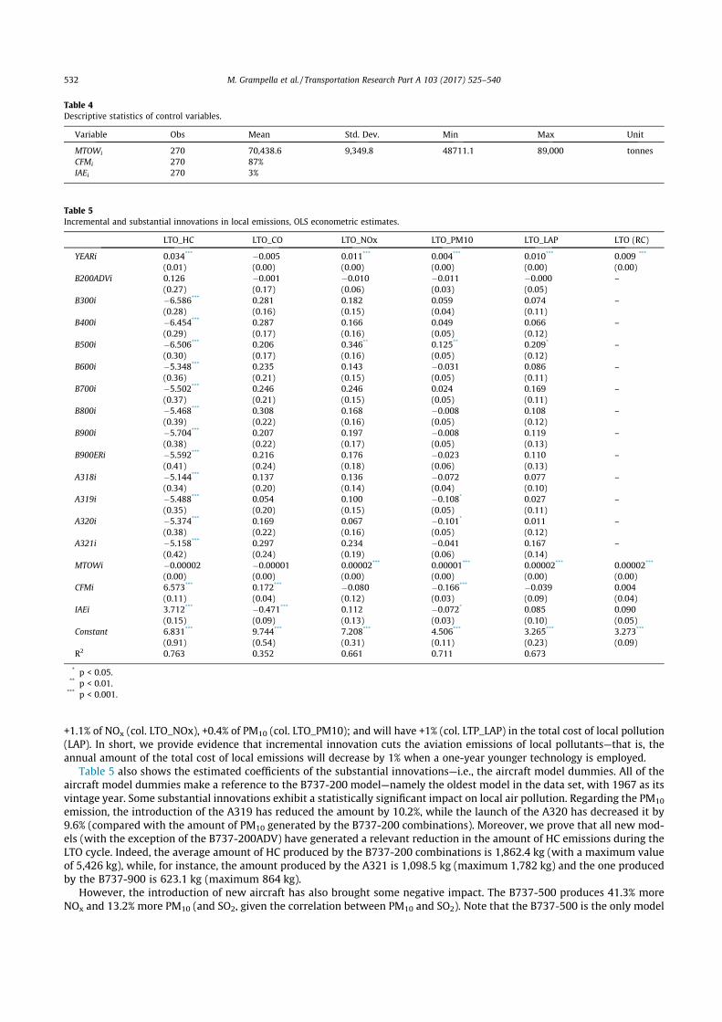
+1.1% of NOx (col. LTO_NOx), +0.4% of PM10 (col. LTO_PM10); and will have +1% (col. LTP_LAP) in the total cost of local pollution(LAP). In short, we provide evidence that incremental innovation cuts the aviation emissions of local pollutants—that is, theannual amount of the total cost of local emissions will decrease by 1% when a one-year younger technology is employed.

Table 5 also shows the estimated coefficients of the substantial innovations—i.e., the aircraft model dummies. All of theaircraft model dummies make a reference to the B737-200 model—namely the oldest model in the data set, with 1967 as itsvintage year. Some substantial innovations exhibit a statistically significant impact on local air pollution. Regarding the PM10

emission, the introduction of the A319 has reduced the amount by 10.2%, while the launch of the A320 has decreased it by9.6% (compared with the amount of PM10 generated by the B737-200 combinations). Moreover, we prove that all new mod-els (with the exception of the B737-200ADV) have generated a relevant reduction in the amount of HC emissions during theLTO cycle. Indeed, the average amount of HC produced by the B737-200 combinations is 1,862.4 kg (with a maximum valueof 5,426 kg), while, for instance, the amount produced by the A321 is 1,098.5 kg (maximum 1,782 kg) and the one producedby the B737-900 is 623.1 kg (maximum 864 kg).

However, the introduction of new aircraft has also brought some negative impact. The B737-500 produces 41.3% moreNOx and 13.2% more PM10 (and SO2, given the correlation between PM10 and SO2). Note that the B737-500 is the only model

Table 4Descriptive statistics of control variables.

Variable Obs Mean Std. Dev. Min Max Unit

MTOWi 270 70,438.6 9,349.8 48711.1 89,000 tonnesCFMi 270 87%IAEi 270 3%

Table 5Incremental and substantial innovations in local emissions, OLS econometric estimates.

LTO_HC LTO_CO LTO_NOx LTO_PM10 LTO_LAP LTO (RC)

YEARi 0.034*** #0.005 0.011*** 0.004*** 0.010*** 0.009 ***

(0.01) (0.00) (0.00) (0.00) (0.00) (0.00)B200ADVi 0.126 #0.001 #0.010 #0.011 #0.000 –

(0.27) (0.17) (0.06) (0.03) (0.05)B300i #6.586*** 0.281 0.182 0.059 0.074 –

(0.28) (0.16) (0.15) (0.04) (0.11)B400i #6.454*** 0.287 0.166 0.049 0.066 –

(0.29) (0.17) (0.16) (0.05) (0.12)B500i #6.506*** 0.206 0.346** 0.125** 0.209* –

(0.30) (0.17) (0.16) (0.05) (0.12)B600i #5.348*** 0.235 0.143 #0.031 0.086 –

(0.36) (0.21) (0.15) (0.05) (0.11)B700i #5.502*** 0.246 0.246 0.024 0.169 –

(0.37) (0.21) (0.15) (0.05) (0.11)B800i #5.468*** 0.308 0.168 #0.008 0.108 –

(0.39) (0.22) (0.16) (0.05) (0.12)B900i #5.704*** 0.207 0.197 #0.008 0.119 –

(0.38) (0.22) (0.17) (0.05) (0.13)B900ERi #5.592*** 0.216 0.176 #0.023 0.110 –

(0.41) (0.24) (0.18) (0.06) (0.13)A318i #5.144*** 0.137 0.136 #0.072 0.077 –

(0.34) (0.20) (0.14) (0.04) (0.10)A319i #5.488*** 0.054 0.100 #0.108* 0.027 –

(0.35) (0.20) (0.15) (0.05) (0.11)A320i #5.374*** 0.169 0.067 #0.101* 0.011 –

(0.38) (0.22) (0.16) (0.05) (0.12)A321i #5.158*** 0.297 0.234 #0.041 0.167 –

(0.42) (0.24) (0.19) (0.06) (0.14)MTOWi #0.00002 #0.00001 0.00002*** 0.00001*** 0.00002*** 0.00002***

(0.00) (0.00) (0.00) (0.00) (0.00) (0.00)CFMi 6.573*** 0.172*** #0.080 #0.166*** #0.039 0.004

(0.11) (0.04) (0.12) (0.03) (0.09) (0.04)IAEi 3.712*** #0.471*** 0.112 #0.072* 0.085 0.090

(0.15) (0.09) (0.13) (0.03) (0.10) (0.05)Constant 6.831*** 9.744*** 7.208*** 4.506*** 3.265*** 3.273***

(0.91) (0.54) (0.31) (0.11) (0.23) (0.09)R2 0.763 0.352 0.661 0.711 0.673

* p < 0.05.** p < 0.01.*** p < 0.001.


exhibiting the wrong direction, but has a statistically significant effect on the total cost of local pollution, which is increasedby 23.2% in comparison with the older B737-200. In general, no statistical significant evidence exists that substantial inno-vations have, ceteris paribus, had an impact on the total cost of local emissions.

Regarding the control variables, aircraft size (MTOW) has a small but statistically significant effect on the emission of NOx,PM10 (and SO2), and total local emission costs. A larger aircraft size (i.e., an increase of 1 tonne in MTOW) induces a +0.002%increase in the amount of NOx, a +0.001% increase in that of PM10 (and of SO2), and a +0.002% in the total LAP cost. If theengine is provided by the manufacturers CFM and IAE, we obtain estimates of 15.3% and 6.9% lower levels of PM10 respec-tively, but higher HC levels, which leads to a non-significant aggregate effect at the LAP cost level. The goodness of fit (R2) israther high in all regressions.

The last column of Table 5 is included as a robustness check (RC) for the effect of incremental innovation. Both the sig-nificance and the sign of YEAR are also confirmedwhen the dummies representing substantial innovations are excluded fromthe model.20

To conclude, although the empirical analysis on local emissions provides robust evidence that an incremental innovationeffect exists, which is quantified in a#1% annual reduction, there is no evidence of a substantial innovation effect at the flightlevel.

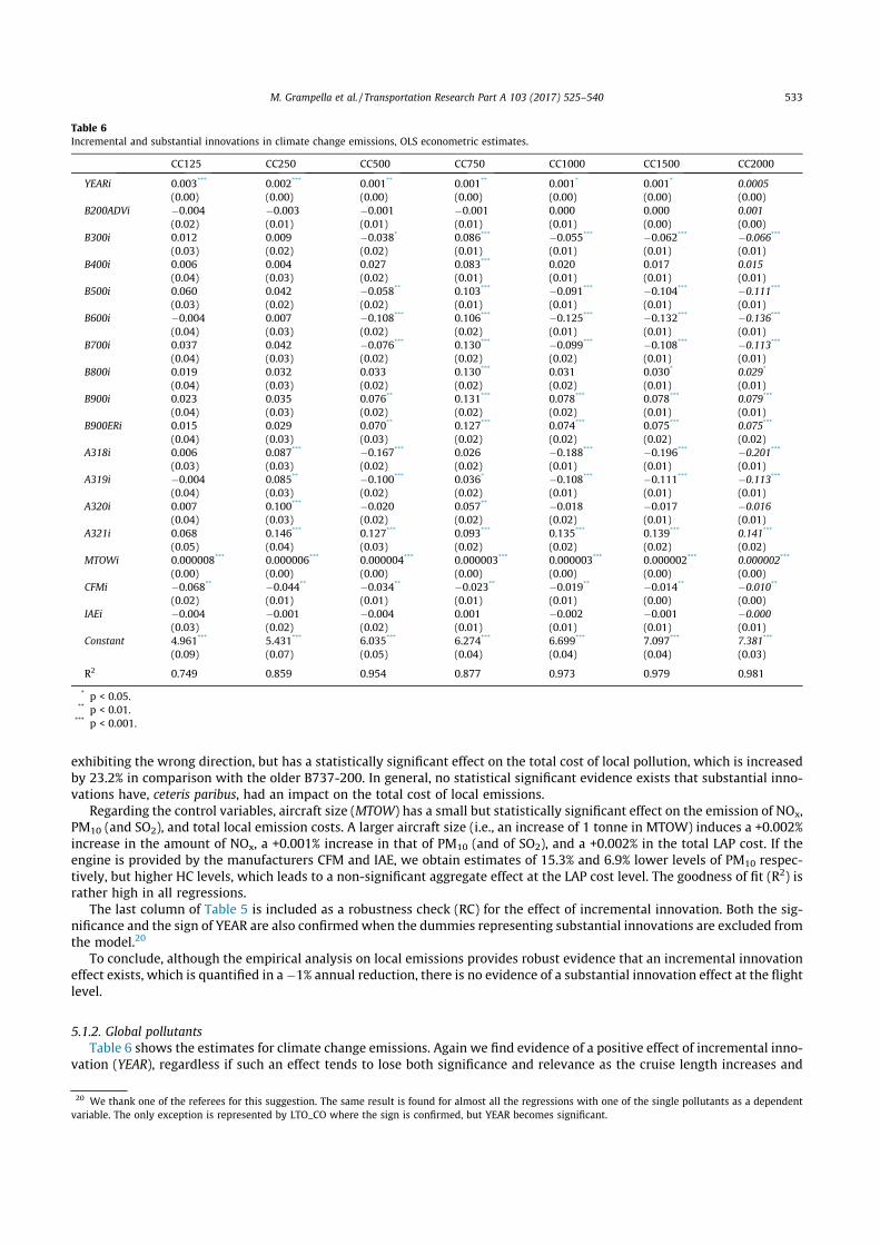
5.1.2. Global pollutantsTable 6 shows the estimates for climate change emissions. Again we find evidence of a positive effect of incremental inno-

vation (YEAR), regardless if such an effect tends to lose both significance and relevance as the cruise length increases and

Table 6Incremental and substantial innovations in climate change emissions, OLS econometric estimates.

CC125 CC250 CC500 CC750 CC1000 CC1500 CC2000

YEARi 0.003*** 0.002*** 0.001** 0.001** 0.001* 0.001* 0.0005(0.00) (0.00) (0.00) (0.00) (0.00) (0.00) (0.00)

B200ADVi #0.004 #0.003 #0.001 #0.001 0.000 0.000 0.001(0.02) (0.01) (0.01) (0.01) (0.01) (0.00) (0.00)

B300i 0.012 0.009 #0.038* 0.086*** #0.055*** #0.062*** #0.066***

(0.03) (0.02) (0.02) (0.01) (0.01) (0.01) (0.01)B400i 0.006 0.004 0.027 0.083*** 0.020 0.017 0.015

(0.04) (0.03) (0.02) (0.01) (0.01) (0.01) (0.01)B500i 0.060 0.042 #0.058** 0.103*** #0.091*** #0.104*** #0.111***

(0.03) (0.02) (0.02) (0.01) (0.01) (0.01) (0.01)B600i #0.004 0.007 #0.108*** 0.106*** #0.125*** #0.132*** #0.136***

(0.04) (0.03) (0.02) (0.02) (0.01) (0.01) (0.01)B700i 0.037 0.042 #0.076*** 0.130*** #0.099*** #0.108*** #0.113***

(0.04) (0.03) (0.02) (0.02) (0.02) (0.01) (0.01)B800i 0.019 0.032 0.033 0.130*** 0.031 0.030* 0.029*

(0.04) (0.03) (0.02) (0.02) (0.02) (0.01) (0.01)B900i 0.023 0.035 0.076** 0.131*** 0.078*** 0.078*** 0.079***

(0.04) (0.03) (0.02) (0.02) (0.02) (0.01) (0.01)B900ERi 0.015 0.029 0.070** 0.127*** 0.074*** 0.075*** 0.075***

(0.04) (0.03) (0.03) (0.02) (0.02) (0.02) (0.02)A318i 0.006 0.087*** #0.167*** 0.026 #0.188*** #0.196*** #0.201***

(0.03) (0.03) (0.02) (0.02) (0.01) (0.01) (0.01)A319i #0.004 0.085** #0.100*** 0.036* #0.108*** #0.111*** #0.113***

(0.04) (0.03) (0.02) (0.02) (0.01) (0.01) (0.01)A320i 0.007 0.100*** #0.020 0.057** #0.018 #0.017 #0.016

(0.04) (0.03) (0.02) (0.02) (0.02) (0.01) (0.01)A321i 0.068 0.146*** 0.127*** 0.093*** 0.135*** 0.139*** 0.141***

(0.05) (0.04) (0.03) (0.02) (0.02) (0.02) (0.02)MTOWi 0.000008*** 0.000006*** 0.000004*** 0.000003*** 0.000003*** 0.000002*** 0.000002***

(0.00) (0.00) (0.00) (0.00) (0.00) (0.00) (0.00)CFMi #0.068** #0.044** #0.034** #0.023** #0.019** #0.014** #0.010**

(0.02) (0.01) (0.01) (0.01) (0.01) (0.00) (0.00)IAEi #0.004 #0.001 #0.004 0.001 #0.002 #0.001 #0.000

(0.03) (0.02) (0.02) (0.01) (0.01) (0.01) (0.01)Constant 4.961*** 5.431*** 6.035*** 6.274*** 6.699*** 7.097*** 7.381***

(0.09) (0.07) (0.05) (0.04) (0.04) (0.04) (0.03)

R2 0.749 0.859 0.954 0.877 0.973 0.979 0.981

* p < 0.05.** p < 0.01.*** p < 0.001.

20 We thank one of the referees for this suggestion. The same result is found for almost all the regressions with one of the single pollutants as a dependentvariable. The only exception is represented by LTO_CO where the sign is confirmed, but YEAR becomes significant.


becomes statistically insignificant at the longest length (2000 nm). Further, climate change cost reductions range between#0.3% for a 125-nm stage length and #0.1% for a 1500-nm stage length. This may be due to the fact that technical progressmainly affects emissions produced at the ascent—namely, the phase generating the highest amount of pollution—andreduces as the flight distance increases.

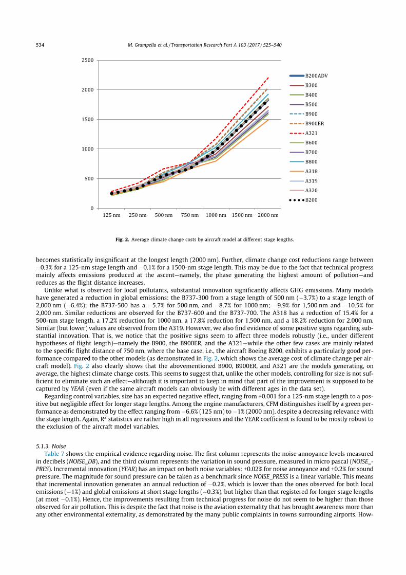
Unlike what is observed for local pollutants, substantial innovation significantly affects GHG emissions. Many modelshave generated a reduction in global emissions: the B737-300 from a stage length of 500 nm (#3.7%) to a stage length of2,000 nm (#6.4%); the B737-500 has a #5.7% for 500 nm, and #8.7% for 1000 nm; #9.9% for 1,500 nm and #10.5% for2,000 nm. Similar reductions are observed for the B737-600 and the B737-700. The A318 has a reduction of 15.4% for a500-nm stage length, a 17.2% reduction for 1000 nm, a 17.8% reduction for 1,500 nm, and a 18.2% reduction for 2,000 nm.Similar (but lower) values are observed from the A319. However, we also find evidence of some positive signs regarding sub-stantial innovation. That is, we notice that the positive signs seem to affect three models robustly (i.e., under differenthypotheses of flight length)—namely the B900, the B900ER, and the A321—while the other few cases are mainly relatedto the specific flight distance of 750 nm, where the base case, i.e., the aircraft Boeing B200, exhibits a particularly good per-formance compared to the other models (as demonstrated in Fig. 2, which shows the average cost of climate change per air-craft model). Fig. 2 also clearly shows that the abovementioned B900, B900ER, and A321 are the models generating, onaverage, the highest climate change costs. This seems to suggest that, unlike the other models, controlling for size is not suf-ficient to eliminate such an effect—although it is important to keep in mind that part of the improvement is supposed to becaptured by YEAR (even if the same aircraft models can obviously be with different ages in the data set).

Regarding control variables, size has an expected negative effect, ranging from +0.001 for a 125-nm stage length to a pos-itive but negligible effect for longer stage lengths. Among the engine manufacturers, CFM distinguishes itself by a green per-formance as demonstrated by the effect ranging from #6.6% (125 nm) to#1% (2000 nm), despite a decreasing relevance withthe stage length. Again, R2 statistics are rather high in all regressions and the YEAR coefficient is found to be mostly robust tothe exclusion of the aircraft model variables.

5.1.3. NoiseTable 7 shows the empirical evidence regarding noise. The first column represents the noise annoyance levels measured

in decibels (NOISE_DB), and the third column represents the variation in sound pressure, measured in micro pascal (NOISE_-PRES). Incremental innovation (YEAR) has an impact on both noise variables: +0.02% for noise annoyance and +0.2% for soundpressure. The magnitude for sound pressure can be taken as a benchmark since NOISE_PRESS is a linear variable. This meansthat incremental innovation generates an annual reduction of #0.2%, which is lower than the ones observed for both localemissions (#1%) and global emissions at short stage lengths (#0.3%), but higher than that registered for longer stage lengths(at most #0.1%). Hence, the improvements resulting from technical progress for noise do not seem to be higher than thoseobserved for air pollution. This is despite the fact that noise is the aviation externality that has brought awareness more thanany other environmental externality, as demonstrated by the many public complaints in towns surrounding airports. How-

0500

1000150020002500

125 nm 250 nm 500 nm 750 nm 1000 nm 1500 nm 2000 nm

B200ADVB300B400B500B900B900ERA321B600B700B800A318A319A320B200

Fig. 2. Average climate change costs by aircraft model at different stage lengths.


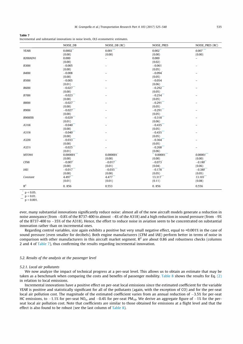
ever, many substantial innovations significantly reduce noise: almost all of the new aircraft models generate a reduction innoise annoyance (from #0.8% of the B737-400 to almost #4% of the A318) and a high reduction in sound pressure (from #9%of the B737-400 to #35% of the A318). Hence, the effort to reduce noise in aviation seem to be concentrated on substantialinnovation rather than on incremental ones.

Regarding control variables, size again exhibits a positive but very small negative effect, equal to +0.001% in the case ofsound pressure (even smaller for decibels). Both engine manufacturers (CFM and IAE) perform better in terms of noise incomparison with other manufacturers in this aircraft market segment. R2 are about 0.86 and robustness checks (columns2 and 4 of Table 7), thus confirming the results regarding incremental innovation.

5.2. Results of the analysis at the passenger level

5.2.1. Local air pollutantsWe now analyze the impact of technical progress at a per-seat level. This allows us to obtain an estimate that may be

taken as a benchmark when comparing the costs and benefits of passenger mobility. Table 8 shows the results for Eq. (2)in relation to local emissions.

Incremental innovations have a positive effect on per-seat local emissions since the estimated coefficient for the variableYEAR is positive and statistically significant for all of the pollutants (again, with the exception of CO) and for the per-seatlocal air pollution cost. The magnitude of the estimated coefficient varies from an annual reduction of #3.5% for per-seatHC emissions, to #1.1% for per-seat NOx, and #0.4% for per-seat PM10. We derive an aggregate figure of #1% for the per-seat local air pollution cost. Note that coefficients are similar to those obtained for emissions at a flight level and that theeffect is also found to be robust (see the last column of Table 8).

Table 7Incremental and substantial innovations in noise levels, OLS econometric estimates.

NOISE_DB NOISE_DB (RC) NOISE_PRES NOISE_PRES (RC)

YEARi 0.0002** 0.001*** 0.002** 0.007 ***

(0.00) (0.00) (0.00) (0.00)B200ADVi 0.000 – 0.000 –

(0.00) (0.02)B300i #0.005 – #0.061 –

(0.00) (0.05)B400i #0.008 – #0.094* –

(0.00) (0.05)B500i #0.005 – #0.054 –

(0.01) (0.06)B600i #0.027*** – #0.292*** –

(0.00) (0.05)B700i #0.023*** – #0.254*** –

(0.00) (0.05)B800i #0.027*** – #0.291*** –

(0.00) (0.05)B900i #0.027*** – #0.291*** –

(0.00) (0.05)B900ERi #0.029*** – #0.318*** –

(0.01) (0.06)A318i #0.040*** – #0.435*** –

(0.00) (0.05)A319i #0.040*** – #0.435*** –

(0.00) (0.05)A320i #0.033*** – #0.364*** –

(0.00) (0.05)A321i #0.025*** – #0.268*** –

(0.01) (0.06)MTOWi 0.000001*** 0.000001* ** 0.00001*** 0.00001***

(0.00) (0.00) (0.00) (0.00)CFMi #0.007* #0.017** #0.073* #0.180**

(0.00) (0.01) (0.04) (0.06)IAEi #0.017*** #0.035*** #0.178*** #0.380***

(0.00) (0.00) (0.05) (0.05)Constant 4.497*** 4.477*** 13.317*** 13.103***

(0.01) (0.01) (0.11) (0.08)

R2 0. 856 0.553 0. 856 0.556

* p < 0.05.** p < 0.01.*** p < 0.001.


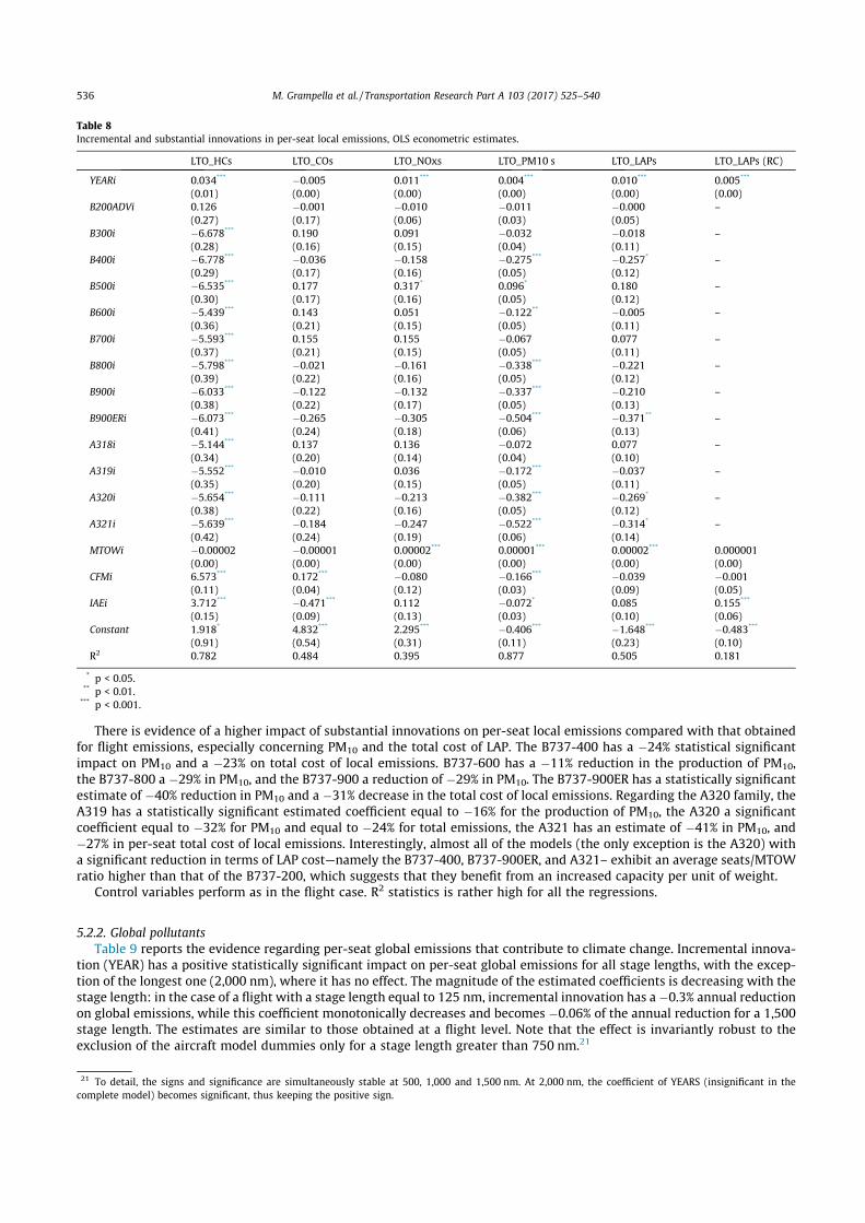
There is evidence of a higher impact of substantial innovations on per-seat local emissions compared with that obtainedfor flight emissions, especially concerning PM10 and the total cost of LAP. The B737-400 has a #24% statistical significantimpact on PM10 and a #23% on total cost of local emissions. B737-600 has a #11% reduction in the production of PM10,the B737-800 a #29% in PM10, and the B737-900 a reduction of #29% in PM10. The B737-900ER has a statistically significantestimate of #40% reduction in PM10 and a #31% decrease in the total cost of local emissions. Regarding the A320 family, theA319 has a statistically significant estimated coefficient equal to #16% for the production of PM10, the A320 a significantcoefficient equal to #32% for PM10 and equal to #24% for total emissions, the A321 has an estimate of #41% in PM10, and#27% in per-seat total cost of local emissions. Interestingly, almost all of the models (the only exception is the A320) witha significant reduction in terms of LAP cost—namely the B737-400, B737-900ER, and A321– exhibit an average seats/MTOWratio higher than that of the B737-200, which suggests that they benefit from an increased capacity per unit of weight.

Control variables perform as in the flight case. R2 statistics is rather high for all the regressions.

5.2.2. Global pollutantsTable 9 reports the evidence regarding per-seat global emissions that contribute to climate change. Incremental innova-

tion (YEAR) has a positive statistically significant impact on per-seat global emissions for all stage lengths, with the excep-tion of the longest one (2,000 nm), where it has no effect. The magnitude of the estimated coefficients is decreasing with thestage length: in the case of a flight with a stage length equal to 125 nm, incremental innovation has a#0.3% annual reductionon global emissions, while this coefficient monotonically decreases and becomes #0.06% of the annual reduction for a 1,500stage length. The estimates are similar to those obtained at a flight level. Note that the effect is invariantly robust to theexclusion of the aircraft model dummies only for a stage length greater than 750 nm.21

Table 8Incremental and substantial innovations in per-seat local emissions, OLS econometric estimates.

LTO_HCs LTO_COs LTO_NOxs LTO_PM10 s LTO_LAPs LTO_LAPs (RC)

YEARi 0.034*** #0.005 0.011*** 0.004*** 0.010*** 0.005***

(0.01) (0.00) (0.00) (0.00) (0.00) (0.00)B200ADVi 0.126 #0.001 #0.010 #0.011 #0.000 –

(0.27) (0.17) (0.06) (0.03) (0.05)B300i #6.678*** 0.190 0.091 #0.032 #0.018 –

(0.28) (0.16) (0.15) (0.04) (0.11)B400i #6.778*** #0.036 #0.158 #0.275*** #0.257* –

(0.29) (0.17) (0.16) (0.05) (0.12)B500i #6.535*** 0.177 0.317* 0.096* 0.180 –

(0.30) (0.17) (0.16) (0.05) (0.12)B600i #5.439*** 0.143 0.051 #0.122** #0.005 –

(0.36) (0.21) (0.15) (0.05) (0.11)B700i #5.593*** 0.155 0.155 #0.067 0.077 –

(0.37) (0.21) (0.15) (0.05) (0.11)B800i #5.798*** #0.021 #0.161 #0.338*** #0.221 –

(0.39) (0.22) (0.16) (0.05) (0.12)B900i #6.033*** #0.122 #0.132 #0.337*** #0.210 –

(0.38) (0.22) (0.17) (0.05) (0.13)B900ERi #6.073*** #0.265 #0.305 #0.504*** #0.371** –

(0.41) (0.24) (0.18) (0.06) (0.13)A318i #5.144*** 0.137 0.136 #0.072 0.077 –

(0.34) (0.20) (0.14) (0.04) (0.10)A319i #5.552*** #0.010 0.036 #0.172*** #0.037 –

(0.35) (0.20) (0.15) (0.05) (0.11)A320i #5.654*** #0.111 #0.213 #0.382*** #0.269* –

(0.38) (0.22) (0.16) (0.05) (0.12)A321i #5.639*** #0.184 #0.247 #0.522*** #0.314* –

(0.42) (0.24) (0.19) (0.06) (0.14)MTOWi #0.00002 #0.00001 0.00002*** 0.00001*** 0.00002*** 0.000001

(0.00) (0.00) (0.00) (0.00) (0.00) (0.00)CFMi 6.573*** 0.172*** #0.080 #0.166*** #0.039 #0.001

(0.11) (0.04) (0.12) (0.03) (0.09) (0.05)IAEi 3.712*** #0.471*** 0.112 #0.072* 0.085 0.155***

(0.15) (0.09) (0.13) (0.03) (0.10) (0.06)Constant 1.918* 4.832*** 2.295*** #0.406*** #1.648*** #0.483***

(0.91) (0.54) (0.31) (0.11) (0.23) (0.10)R2 0.782 0.484 0.395 0.877 0.505 0.181

* p < 0.05.** p < 0.01.*** p < 0.001.

21 To detail, the signs and significance are simultaneously stable at 500, 1,000 and 1,500 nm. At 2,000 nm, the coefficient of YEARS (insignificant in thecomplete model) becomes significant, thus keeping the positive sign.


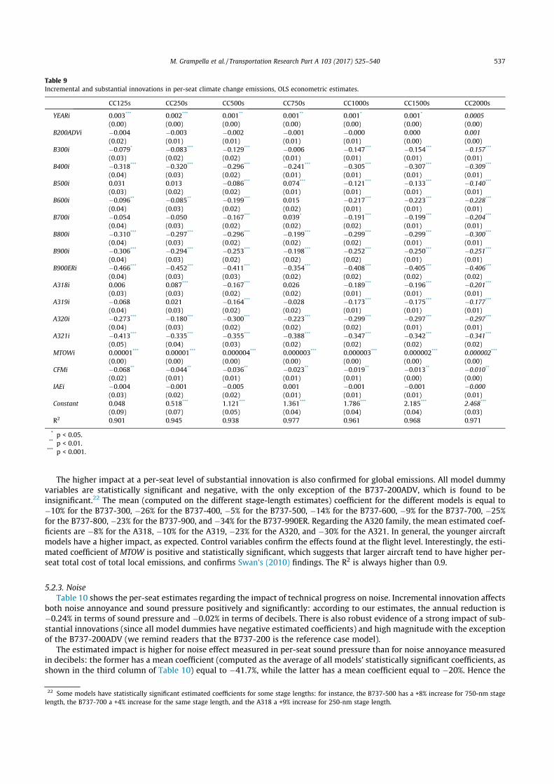
The higher impact at a per-seat level of substantial innovation is also confirmed for global emissions. All model dummyvariables are statistically significant and negative, with the only exception of the B737-200ADV, which is found to beinsignificant.22 The mean (computed on the different stage-length estimates) coefficient for the different models is equal to#10% for the B737-300, #26% for the B737-400, #5% for the B737-500, #14% for the B737-600, #9% for the B737-700, #25%for the B737-800, #23% for the B737-900, and #34% for the B737-990ER. Regarding the A320 family, the mean estimated coef-ficients are #8% for the A318, #10% for the A319, #23% for the A320, and #30% for the A321. In general, the younger aircraftmodels have a higher impact, as expected. Control variables confirm the effects found at the flight level. Interestingly, the esti-mated coefficient of MTOW is positive and statistically significant, which suggests that larger aircraft tend to have higher per-seat total cost of total local emissions, and confirms Swan’s (2010) findings. The R2 is always higher than 0.9.

5.2.3. NoiseTable 10 shows the per-seat estimates regarding the impact of technical progress on noise. Incremental innovation affects

both noise annoyance and sound pressure positively and significantly: according to our estimates, the annual reduction is#0.24% in terms of sound pressure and #0.02% in terms of decibels. There is also robust evidence of a strong impact of sub-stantial innovations (since all model dummies have negative estimated coefficients) and high magnitude with the exceptionof the B737-200ADV (we remind readers that the B737-200 is the reference case model).

The estimated impact is higher for noise effect measured in per-seat sound pressure than for noise annoyance measuredin decibels: the former has a mean coefficient (computed as the average of all models’ statistically significant coefficients, asshown in the third column of Table 10) equal to #41.7%, while the latter has a mean coefficient equal to #20%. Hence the

Table 9Incremental and substantial innovations in per-seat climate change emissions, OLS econometric estimates.

CC125s CC250s CC500s CC750s CC1000s CC1500s CC2000s

YEARi 0.003*** 0.002*** 0.001** 0.001** 0.001* 0.001* 0.0005(0.00) (0.00) (0.00) (0.00) (0.00) (0.00) (0.00)

B200ADVi #0.004 #0.003 #0.002 #0.001 #0.000 0.000 0.001(0.02) (0.01) (0.01) (0.01) (0.01) (0.00) (0.00)

B300i #0.079* #0.083*** #0.129*** #0.006 #0.147*** #0.154*** #0.157***

(0.03) (0.02) (0.02) (0.01) (0.01) (0.01) (0.01)B400i #0.318*** #0.320*** #0.296*** #0.241*** #0.305*** #0.307*** #0.309***

(0.04) (0.03) (0.02) (0.01) (0.01) (0.01) (0.01)B500i 0.031 0.013 #0.086*** 0.074*** #0.121*** #0.133*** #0.140***

(0.03) (0.02) (0.02) (0.01) (0.01) (0.01) (0.01)B600i #0.096** #0.085** #0.199*** 0.015 #0.217*** #0.223*** #0.228***

(0.04) (0.03) (0.02) (0.02) (0.01) (0.01) (0.01)B700i #0.054 #0.050 #0.167*** 0.039* #0.191*** #0.199*** #0.204***

(0.04) (0.03) (0.02) (0.02) (0.02) (0.01) (0.01)B800i #0.310*** #0.297*** #0.296*** #0.199*** #0.299*** #0.299*** #0.300***

(0.04) (0.03) (0.02) (0.02) (0.02) (0.01) (0.01)B900i #0.306*** #0.294*** #0.253*** #0.198*** #0.252*** #0.250*** #0.251***

(0.04) (0.03) (0.02) (0.02) (0.02) (0.01) (0.01)B900ERi #0.466*** #0.452*** #0.411*** #0.354*** #0.408*** #0.405*** #0.406***

(0.04) (0.03) (0.03) (0.02) (0.02) (0.02) (0.02)A318i 0.006 0.087*** #0.167*** 0.026 #0.189*** #0.196*** #0.201***

(0.03) (0.03) (0.02) (0.02) (0.01) (0.01) (0.01)A319i #0.068 0.021 #0.164*** #0.028 #0.173*** #0.175*** #0.177***

(0.04) (0.03) (0.02) (0.02) (0.01) (0.01) (0.01)A320i #0.273*** #0.180*** #0.300*** #0.223*** #0.299*** #0.297*** #0.297***

(0.04) (0.03) (0.02) (0.02) (0.02) (0.01) (0.01)A321i #0.413*** #0.335*** #0.355*** #0.388*** #0.347*** #0.342*** #0.341***

(0.05) (0.04) (0.03) (0.02) (0.02) (0.02) (0.02)MTOWi 0.00001*** 0.00001*** 0.000004*** 0.000003*** 0.000003*** 0.000002*** 0.000002***

(0.00) (0.00) (0.00) (0.00) (0.00) (0.00) (0.00)CFMi #0.068** #0.044** #0.036** #0.023** #0.019** #0.013** #0.010**

(0.02) (0.01) (0.01) (0.01) (0.01) (0.00) (0.00)IAEi #0.004 #0.001 #0.005 0.001 #0.001 #0.001 #0.000

(0.03) (0.02) (0.02) (0.01) (0.01) (0.01) (0.01)Constant 0.048 0.518*** 1.121*** 1.361*** 1.786*** 2.185*** 2.468***

(0.09) (0.07) (0.05) (0.04) (0.04) (0.04) (0.03)R2 0.901 0.945 0.938 0.977 0.961 0.968 0.971

* p < 0.05.** p < 0.01.*** p < 0.001.

22 Some models have statistically significant estimated coefficients for some stage lengths: for instance, the B737-500 has a +8% increase for 750-nm stagelength, the B737-700 a +4% increase for the same stage length, and the A318 a +9% increase for 250-nm stage length.


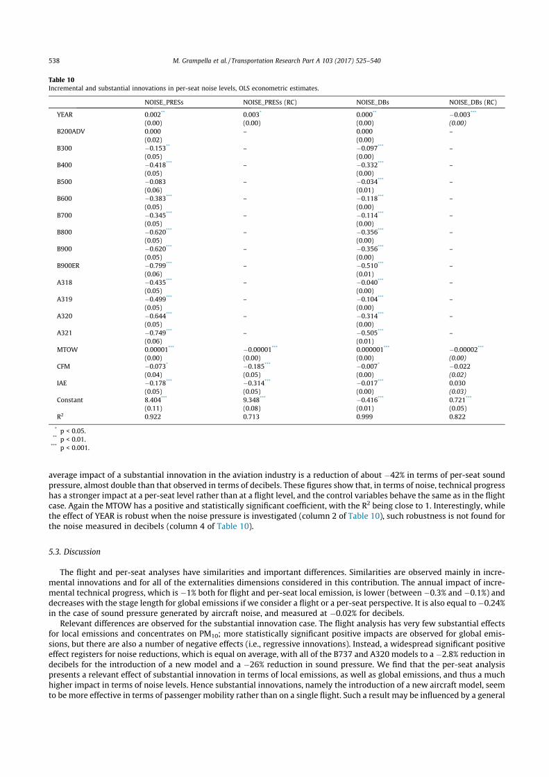
average impact of a substantial innovation in the aviation industry is a reduction of about #42% in terms of per-seat soundpressure, almost double than that observed in terms of decibels. These figures show that, in terms of noise, technical progresshas a stronger impact at a per-seat level rather than at a flight level, and the control variables behave the same as in the flightcase. Again the MTOW has a positive and statistically significant coefficient, with the R2 being close to 1. Interestingly, whilethe effect of YEAR is robust when the noise pressure is investigated (column 2 of Table 10), such robustness is not found forthe noise measured in decibels (column 4 of Table 10).

5.3. Discussion

The flight and per-seat analyses have similarities and important differences. Similarities are observed mainly in incre-mental innovations and for all of the externalities dimensions considered in this contribution. The annual impact of incre-mental technical progress, which is #1% both for flight and per-seat local emission, is lower (between #0.3% and #0.1%) anddecreases with the stage length for global emissions if we consider a flight or a per-seat perspective. It is also equal to #0.24%in the case of sound pressure generated by aircraft noise, and measured at #0.02% for decibels.

Relevant differences are observed for the substantial innovation case. The flight analysis has very few substantial effectsfor local emissions and concentrates on PM10; more statistically significant positive impacts are observed for global emis-sions, but there are also a number of negative effects (i.e., regressive innovations). Instead, a widespread significant positiveeffect registers for noise reductions, which is equal on average, with all of the B737 and A320 models to a #2.8% reduction indecibels for the introduction of a new model and a #26% reduction in sound pressure. We find that the per-seat analysispresents a relevant effect of substantial innovation in terms of local emissions, as well as global emissions, and thus a muchhigher impact in terms of noise levels. Hence substantial innovations, namely the introduction of a new aircraft model, seemto be more effective in terms of passenger mobility rather than on a single flight. Such a result may be influenced by a general

Table 10Incremental and substantial innovations in per-seat noise levels, OLS econometric estimates.

NOISE_PRESs NOISE_PRESs (RC) NOISE_DBs NOISE_DBs (RC)

YEAR 0.002** 0.003* 0.000** #0.003***

(0.00) (0.00) (0.00) (0.00)B200ADV 0.000 – 0.000 –

(0.02) (0.00)B300 #0.153** – #0.097*** –

(0.05) (0.00)B400 #0.418*** – #0.332*** –

(0.05) (0.00)B500 #0.083 – #0.034*** –

(0.06) (0.01)B600 #0.383*** – #0.118*** –

(0.05) (0.00)B700 #0.345*** – #0.114*** –

(0.05) (0.00)B800 #0.620*** – #0.356*** –

(0.05) (0.00)B900 #0.620*** – #0.356*** –

(0.05) (0.00)B900ER #0.799*** – #0.510*** –

(0.06) (0.01)A318 #0.435*** – #0.040*** –

(0.05) (0.00)A319 #0.499*** – #0.104*** –

(0.05) (0.00)A320 #0.644*** – #0.314*** –

(0.05) (0.00)A321 #0.749*** – #0.505*** –

(0.06) (0.01)MTOW 0.00001*** #0.00001*** 0.000001*** #0.00002***

(0.00) (0.00) (0.00) (0.00)CFM #0.073* #0.185*** #0.007* #0.022

(0.04) (0.05) (0.00) (0.02)IAE #0.178*** #0.314*** #0.017*** 0.030

(0.05) (0.05) (0.00) (0.03)Constant 8.404*** 9.348*** #0.416*** 0.721***

(0.11) (0.08) (0.01) (0.05)R2 0.922 0.713 0.999 0.822

* p < 0.05.** p < 0.01.*** p < 0.001.


shift toward aircraft with a greater capacity. Note that in most of the cases, a new aircraft model is characterized by (1) areduced environmental impact (e.g., due to increased fuel efficiency), and (2) an increased capacity in terms of availableseats. Despite the correlation between capacity (seats) and size (MTOW), aircraft with the same MTOW provide differentcapacities. In other words, the per-seat pollution incorporates the ability to transport a higher number of passengers witha less-than-proportional increase in the weight (with respect to the previous technology). Our result suggests that this ‘‘ef-ficiency” is often related to the introduction of a new aircraft model.

Last, we obtain very sparse evidence on the existence of a trade-off between emissions and noise. We find contrastingeffects on global emissions and noise levels only for some substantial innovations: the B737-400, the B737-800, theB737-900, the B737-900ER and the A321 have all had a bad impact on global emissions in many stage lengths consideredhere, although they show a robust reduction in noise levels. However, excluding these cases (and only for some stagelengths), we do not observe a conflicting effect of both incremental and substantial technical progress between emissionsand noise, which is a different finding than that of Phleps and Hornung (2013).

6. Conclusions

This paper investigates a data set composed of 270 different aircraft/engine combinations belonging to the B737 and A320families, with a twofold goal: (1) to provide econometric evidence of the impact of both incremental and substantial tech-nical progress on aviation externalities (i.e., both local and global emissions) and noise; and (2) to analyze whether innova-tion impacts in different ways flight externalities (i.e., the amount of pollution and noise generated by a flight operated by aspecific aircraft/engine combination) and per-passenger externalities.

Incremental technical progress is embedded in the age of an aircraft/engine combination, while substantial innovationrefers to the introduction of a new aircraft model (i.e., a new version of a B737; we consider 10 successive versions startingfrom year 1967 to year 2010. Regarding the A320, we consider 4 successive versions from year 1996 to 2006).

Our results show a general statistically significant impact of incremental technical progress. A one-year younger aircraft/engine combination leads to (i) #1% in terms of local pollution, (ii) a reduction ranging from #0.3% to #0.1% in terms of glo-bal pollution (that diminishes as stage length increases), and (iii) #0.24% and #0.022%, respectively, in sound pressure anddecibels. Per-flight and per-passenger estimates are similar.

We also present some econometric evidence that although substantial innovation has a limited impact on local and globalflight emissions, it has a significant positive impact on noise level, with an average reduction of #26% of noise when a newmodel is introduced. On the contrary, we find a widespread positive effect of substantial innovations on per-passenger exter-nalities: many new models reduce local emissions (with an average estimated reduction equal to #24% on local totals),almost all new models reduce global emissions (an average effect of about #20% for all investigated stage lengths), whilethere is a strong significant effect of substantial innovations in terms of sound pressure reduction (the average effect is#42%, a smaller effect equal to #20% in terms of noise annoyance measured in decibels). Hence, the stronger effects of inno-vations are observed by looking at passenger mobility, while lower and less widespread effects are observed from theamount of externalities generated by a flight. Such a result may be due to the combined effect of technology improvementand increasing aircraft size/capacity over time. Indeed, a new model tends to have, on average, a greater size that may softenthe possible effect of technological progress on the flight level.

When the per-seat impact is investigated, negative externalities are not only computed at the passenger level, but theyalso incorporate possible gains in terms of seat/weight (capacity/size) ratio. This seems to make the effect of substantialinnovation emerge more clearly. In this sense, it is noteworthy that the per-passenger environmental impact can be reducedeven when the per-flight impact is increased.

The above estimates are different from those found by previous contributions based on computational algorithms and adhoc development scenarios. For instance, Macintosh andWallace (2009) report a 1.9% per year improvement due to technicalprogress regarding only CO2. Chèze et al. (2011a) present a #3% annual reduction in tonnes of jet fuel by available tonnekilometers. Although our estimate is moderate, it is based purely on data and econometric evidence, which is different fromprevious contributions that have focused on algorithms and simulations.

Our results underline the following policy implications. First, if we take into account the forecasts of an annual +4.5%increase in passenger traffic up to the year 2025, as well as a +6.1% increase in cargo traffic (Khandelwal et al., 2013), it isevident that a #1% yearly rate of reduction in emissions is not enough to outweigh the projected increased emissions andcorresponding damage to the environment. For instance, Chèze et al. (2013) show that a 4.7% annual increase in aviationtraffic yields a +1.9% per-year increase in CO2 emissions. When we take this value as reference, a +4.5% annual passengerincrease gives rise to a +1.8% increase in emissions that is not compensated by the #1% reduction in local emission dueto incremental technical progress. Hence, it is essential to introduce policies that may encourage innovation in the aviationsector, so that technological progress happens at a faster pace compared to the current pace. A twice-faster pace of technicalprogress would be enough to suppress the emissions of today’s trends. This confirms the argument by Chèze et al. (2013)that current innovation process in aviation does not guarantee future better performances in terms of emissions.

Second, our estimates may be adopted as benchmarks in aviation charges related to both emission and noise. For instance,emission surcharges may refer to a #1% reduction in local emissions, and, as such, tariffs may be created with penalties ifairlines do not meet such benchmarks. Similarly, the benchmark for a noise surcharge would be a #0.2% annual reduction.


In the case of the more common decibels metric, the benchmark might be a #0.02% annual reduction. Regarding climatechange, emission trading schemes such as the one adopted in the EU may include a dynamic incentive: a #0.1% reductionin global emissions.

This work may be scaled up by an analysis of the entire current commercial fleet, other types of substantial innovations(e.g., the introduction of successive ICAO Annex Chapters), or nonlinear incremental technical progress. Moreover, it may beinteresting to develop a monetary value of noise damage cost that aggregates noise and emission externalities into a singleindex, and thus to study the aggregate impact of technical progress on the total social cost of aviation. These extensions areleft for future research.

References

Brüel & Kjær Sound & Vibration Measurement A/S, 2000. Il rumore ambientale. Nærum, Denmark. https://www.bksv.com/media/doc/br1631.pdf (accessedDecember 2016).

Brugnoli, A., Button, K., Martini, G., Scotti, D., 2015. Economic factors affecting the registration of lower CO2 emitting aircraft in Europe. Transport. Re. Part D:Transp. Environ. 38, 117–124.

Chèze, B., Gastineau, P., Chevallier, J., 2011a. Forecasting world and regional aviation jet fuel demands to the mid-term (2025). Energy Policy 39 (9), 5147–5158.

Chèze, B., Gastineau, P., Chevallier, J., 2011b. Air traffic energy efficiency differs from place to place: new results from a macro-level approach. Economieinternationale 2, 151–178.

Chèze, B., Chevallier, J., Gastineau, P., 2013. Will technological progress be sufficient to stabilize CO2 emissions from air transport in the mid-term?Transport. Res. Part D: Transp. Environ. 18, 91–96.

Dings, J., Wit, R., Leurs, B.D., 2003. External Costs of Aviation. Federal Environmental Agency, Berlin.Givoni, M., Rietveld, P., 2010. The environmental implications of airlines’ choice of aircraft size. J. Air Transp. Manage. 16 (3), 159–167.Grampella, M., Martini, G., Scotti, D., Tassan, F., Zambon, G., 2017. Determinants of airports’ environmental effects. Transport. Res. Part D: Transp. Environ.

50, 327–344.IPCC (1999). Aviation and the Global Atmosphere. IPCC Special Report.Khandelwal, B., Karakurt, A., Sekaran, P.R., Sethi, V., Singh, R., 2013. Hydrogen powered aircraft: the future of air transport. Prog. Aerosp. Sci. 60, 45–59.Lee, D.S., Fahey, D.W., Forster, P.M., Newton, P.J., Wit, R.C., Lim, L.L., et al, 2009. Aviation and global climate change in the 21st century. Atmos. Environ. 43

(22), 3520–3537.Leylekian, L., Lebrun, M., Lempereur, P., 2014. An overview of aircraft noise reduction technologies. AerospaceLab 6, 1–15.Lu, C., 2009. The implications of environmental costs on air passenger demand for different airline business models. J. Air Transport Manage. 15 (4), 158–

165.Lu, C., 2011. The economic benefits and environmental costs of airport operations: Taiwan Taoyuan International Airport. J. Air Transp. Manage. 17 (6), 360–

363.Lu, C., Morrell, P., 2006. Determination and applications of environmental costs at different sized airports–aircraft noise and engine emissions.

Transportation 33 (1), 45–61.Macintosh, A., Wallace, L., 2009. International aviation emissions to 2025: can emissions be stabilized without restricting demand? Energy Policy 37 (1),

264–273.Martini, G., Manello, A., Scotti, D., 2013a. The influence of fleet mix, ownership and LCCs on airports’ technical/environmental efficiency. Transp. Res. Part E

50, 37–52.Martini, G., Scotti, D., Volta, N., 2013b. Including local air pollution in airport efficiency assessment: a hyperbolic stochastic approach. Transport. Res. Part D:

Transp. Environ. 24, 27–36.Miyoshi, C., Mason, K.J., 2009. The carbon emissions of selected airlines and aircraft types in three geographic markets. J. Air Transp. Manage. 15 (3), 138–

147.Morrell, P., Lu, C., 2007. The environmental cost implication of hub–hub versus hub by-pass flight networks. Transport. Res. Part D: Transp. Environ. 12 (3),

143–157.Passchier-Vermeer, W., Passchier, W.F., 2000. Noise exposure and public health. Environ. Health Perspect. 108 (Suppl 1), 123.Phleps, P., Hornung, M., 2013. Noise and emission targeted economic trade-off for next generation single-aisle aircraft. J. Air Transp. Manage. 26, 14–19.Schipper, Y., 2004. Environmental costs in European aviation. Transp. Policy 11 (2), 141–154.Scotti, D., Dresner, M., Martini, G., Yu, C., 2014. Incorporating negative externalities into productivity assessments of US airports. Transp. Res. Part A 62, 39–

53.Statista, 2015. Growth-of-global-air-traffic-passenger-demand. Available: <http://www.statista.com/statistics/193533/growth-of-global-air-traffic-

passenger-demand>.Sutkus, D.J., Baughcum, S.L. D.P. DuBois, 2001. Scheduled Civil Aircraft Emission Inventories for 1999; database development and analysis. NASA/CR-2001-

211216, Washington DC.Swan, W. 2010. Fewer Departures Mean More Noise at Airports. Unpublished Paper <http://cyberswans.com/AirlineIndustryPubs/noise/Noise_Impact_by_

Airplane_Size.doc>.


Contents lists available at ScienceDirect

Transport Policy

journal homepage: www.elsevier.com/locate/tranpol

The determinants of CO2 emissions of air transport passenger traffic: Ananalysis of Lombardy (Italy)

Pak Lam Loa,*, Gianmaria Martinib, Flavio Portab, Davide Scottiba Department of Economics, University of Pavia, Via S. Felice 7, 27100, Pavia, ItalybDepartment of Management, Information and Production Engineering, University of Bergamo, Via Pasubio 7, 24044, Dalmine (BG), Italy

A R T I C L E I N F O

Classification: Environmental Issues in AirTransport Industry, Air Transport Policy andRegulation.

Keywords:Aircraft CO2 emissionsClimate changeTechnology progress

A B S T R A C T

We study the determinants of aviation CO2 emissions by designing an econometric model applied to a panel dataset covering all flights departing from Lombardy, Italy over the 1997–2011 period. We consider two dimensionsof CO2 emissions: total and per available seat kilometer. The latter is a measure of emission efficiency. We focuson different categories of determinants: technical progress; aircraft and network carrier management; policy/business decisions that may not be oriented to limiting CO2, but may indirectly affect it by offsetting projectedoutcomes of policies adopted to reduce emissions (e.g., the EU Emission Trading Scheme (ETS) or the ICAOCarbon Offsetting and Reduction Scheme for International Aviation); and others. We find that although aircraftsize increases total emissions, it reduces emissions per available seat kilometers (ASK), while the route distanceincreases total emissions and decreases emissions per ASK, implying that CO2 is less of a problem for long-haulconnections. Technical progress decreases CO2 emissions per ASK with an estimated elasticity equal to −0.06%.Last, liberalization in the EU market has generated the development of low-cost carriers, which in turn havelowered CO2 emission per ASK, that is, liberalization in Europe has brought the collateral effect of reducing theCO2 externality per passenger.

1. Introduction

With an average growth of 5% annually (Vespermann and Wald,2011), global aviation activities play a key role not only in industryperformance and economic development, but also in climate change.Among other pollutants (i.e., NOx, SOx, H2O, soot, PM10, contrails andcirrus), the amount of carbon dioxide (CO2) produced by commercialaviation is substantial. In 2005, CO2 was estimated to be 1.6% of totalanthropogenic radiative forcing (Lee et al., 2009).

According to the Air Transportation Action Group (ATAG)1 theglobal aviation industry, counting over 3 billion air passengers, pro-duced 705 million tons of CO2 in 2013, accounting for 2% of thehuman-induced CO2 emissions and 13% of total transportation-relatedemissions. According to the 2016 European Aviation EnvironmentalReport by European Aviation Safety Agency (EASA), there were 80%more European flights in 2014 compared with the number of flights in1990. This environmental impact has increased regardless of possibletechnology improvements: in 2014, there was +5% more aviation-

induced CO2 with respect to the level in 2005, and +44–53% more CO2

is estimated in 2035.Politicians and regulators have agreed to limit CO2 emissions in

response to public pressure on the issue of climate change. For instance,the 2015 Paris agreement established a temperature increase limit to1.5 °C above pre-industrial levels.2 In 1997, the Kyoto Pro-tocol was signed, and the International Civil Aviation Organization(ICAO) was assigned to lead the establishment of global aviation CO2

regulation. Reaction to this regulation varied among countries. NewZealand and Australia initiated domestic aviation emission trading in2010 and 2012 respectively, while the EU introduced the Aviation Di-rective in 2012 on both intra-EU and extra-EU flights as an extension ofits already implemented Emission Trading Scheme (ETS) in other sec-tors in 2005. Extra-EU flights were then waived after legal action hadbeen brought against the directive by some airlines and the Interna-tional Air Transport Association (IATA)—the so-called “stop the clock”decision that should have stayed enforced until 2016. However, to thebest of our knowledge, the directive is still in force today.

https://doi.org/10.1016/j.tranpol.2018.11.010Received 9 July 2017; Received in revised form 30 September 2018; Accepted 24 November 2018

* Corresponding author.E-mail addresses: [email protected] (P.L. Lo), [email protected] (G. Martini), [email protected] (F. Porta),

[email protected] (D. Scotti).1 ATAG is an independent coalition of organizations and companies of the aviation industry, formed in 1990.2 Paris Agreement, an agreement within the United Nations Framework Convention on Climate Change, is adopted by consensus on 12 December 2015.

7UDQVSRUW�3ROLF\�[[[��[[[[��[[[²[[[

��;��(OVHYLHU�/WG��$OO�ULJKWV�UHVHUYHG�

3OHDVH�FLWH�WKLV�DUWLFOH�DV��/R��3�/��7UDQVSRUW�3ROLF\��KWWSV��GRL�RUJ��M�WUDQSRO��

http://www.sciencedirect.com/science/journal/0967070X

https://www.elsevier.com/locate/tranpol

https://doi.org/10.1016/j.tranpol.2018.11.010


mailto:[email protected]





Pak Lam LO

After several meetings, during its 39th assembly, the ICAO approveda global market-based measurement (GMBM) scheme, the CarbonOffsetting and Reduction Scheme for International Aviation (CORSIA).This type of scheme will be enforced through different phases startingin 2020 (see Scheelhaase et al., 2018, for a detailed discussion).CORSIA, which is different from the EU-ETS, will be applied to allflights, not only flights in the European Economic Area.

Despite the ongoing, time-consuming negotiation process to limitCO2 aviation emissions and reaching a path of environmentally sus-tainable growth, little is still known about factors that affect the amountof CO2 generated by this sector. For instance, Chèze et al. (2011a,2011b) point out that air traffic management (ATM), incremental in-novation in existing aircraft, and substantial innovation (i.e., new air-craft) are the main drivers for reducing aviation emissions, includingCO2. Grampella et al. (2017a) show that a younger aircraft can generate−1% of local emissions per year and −0.3% of global pollution.However, to the best of our knowledge, research on econometric evi-dence of the determinants of CO2 aviation emissions remains lacking.Specifically, a measure of the average flight distance impact on CO2

emissions could provide the fundamentals for designing an ETS that isbased on flight distances rather than a general overall reduction inannual airlines CO2 emissions (equal to 95% of the average historicalaviation emissions during the 2004–2006 period). This per-flight CO2

emissions regulation could provide incentives to airlines for betteraircraft management on different routes. For instance, such regulationscould provide incentives to operate an aircraft fitting current demandson specific routes and thus avoid using aircraft flights with low loadfactors on some routes. Thus, providing an econometric estimate of thesign and magnitude of some factors regarding CO2 aviation emissions isthe first goal of this paper.

Moreover, it is necessary to take into account that CO2 emissionscomprise only one dimension in the air transportation sector, as emis-sions interact with such factors as economic performance, politicalmotives, and regulations on market entry, among others. All of theseother components influence the possible outcomes of decisions adoptedto limit emissions. For instance, although liberalization may boost CO2

emissions by stimulating demand through lower fares, a company re-structuring its network to recover profitability may lead to loweremissions through more efficient ATM. In this paper we aim to considerthe impact of such non-emission specific decisions on the amount ofCO2 generated by aviation. This will provide, if proven, that thesefactors should be included in a cost-benefit analysis that also covers theenvironmental effects (direct and indirect) of a political or managementdecision.

To accomplish this, we exploit three circumstances: (1) the impactof regulation identified by the liberalization of the EU industry; (2) theimpact of political decisions, given by a traffic transfer Act that swapsflights between two airports; and (3) the role of managerial decisionssuch as de-hubbing to reshape the flight network and to recover prof-itability.

We analyze these issues by exploring data on aviation activities andaviation-related CO2 emissions in Italy. Specifically, we focus onLombardy in Northern Italy.3 We design an econometric model toidentify the impact of certain determinants of CO2 aviation emissionsand apply it to a new data set that spans from 1997 to 2011 and consistsof all scheduled flights departing from Lombardy airports in January ofeach year. The per-flight CO2 emissions are based on the aircraft modeland the distance flown.

The effect of non-environment decisions is provided by the esti-mated effect on CO2 emissions of the entry (deregulation) of low-costcarriers (LCCs) when the national government decided in 1998 to im-pose an aircraft-movement cap to one airport (Linate). The decision wasmade to transfer flights to Malpensa in order to have a hub in Lombardy(a political reason). In addition, in 2008, at the apex of one of its re-current financial crisis, Alitalia decided to reshape its network andconcentrate flights at Rome Fiumicino in an attempt to recover profit-ability (a managerial decision).

Each of these factors may have affected CO2 emissions in differentways. For instance, some LCCs could have generated new flights (in-creasing CO2), changing the pattern of air traffic by possibly focusing onshorter routes (decreasing CO2 per passenger), divert passengers fromother CO2-intensive transportation modes (e.g. cars, buses, trucks forfreight), use younger aircraft and generate higher load factors thantraditional carriers, and hence lower CO2 emissions per passenger.4

Similar considerations could be developed for limiting Milan Malpensa(e.g., reshaping both the flight network and the aircraft management)and for Alitalia Malpensa's de-hubbing decision (LCCs may have re-placed Alitalia flights with—if proven—connections using youngeraircraft).

Our period of observation covers 15 years, starting in 1997 andending in 2011. The beginning year allows us to consider the full im-pact of some exogenous decisions (e.g., the 1998 swap from Linate toMalpensa and the impact of liberalization that took place in the mid-2000s). The last year is limited to 2011 for data availability. Althoughwe can look at the three-year period following the Malpensa de-hub-bing to see the effects on CO2 emissions, such a review does not allow usto consider both the impact of recent CO2 regulations such as the EUETS (begun in 2013) and of ICAO CORSIA (approved in 2016).

The paper is organized as follows. Section 2 describes the literaturereview. Section 3 discusses our empirical strategy by computing theper-flight CO2 emissions and presents the econometric model. Section 4describes the available data sets, the data mining process, and de-scriptive statistics in the econometric model variables. Section 5 pre-sents our empirical results, while Section 6 concludes the paper andhighlights some possible policy implications. The Appendix containsassumptions on aircraft models and a list of LCCs defined by the ICAO.


Currently, two main streams of research on aviation externalitiesexist. The first stream focuses on the impact of aviation externalities(mainly emissions and noise) on airports’ vicinity, while the secondstream investigates the future impact of aviation emissions on climatechange using ad-hoc algorithms.

Regarding the first stream, Schipper (2004) conducted a landing/take-off (LTO) cycle assessment and estimation on 1990 data. Vicinityenvironmental costs of European aviation were computed from noise,emissions, and accident risk, and then applied to a set of 36 Europeanmarkets (routes) in a week in 1990. Lu and Morrell (2006) performed asimilar study on four European airports and showed, after computingan aviation externality, that a large part of such externality (noise inthis case) was omitted. Morrell and Lu (2007) compared hub-to-huband hub-bypass networks and found that the latter generated feweremissions than the former. Lu (2009) studied aviation emissions’ chargeeffect on air transportation demand and provided some evidence thatenvironmental surcharges could reduce passenger demand, especiallyin the case of LCCs, even if these carriers impose lower environmentalcosts to passengers. Givoni and Rietveld (2010) investigated narrow-body A320 and wide-body B747 in two routes (London-Amsterdam andTokyo-Sapporo) and showed that higher aircraft size and lower fre-quency generates lower climate change costs but higher local pollution.

3 Lombardy is one of Europe's wealthiest regions and exceeded 10 millionhabitants in 2016. Other than the exceptional tourism volume, Lombardy hasimportant commerce, banking, fashion and design sectors in Milan, as well asstrong industries and agriculture in Bergamo. Lombardy is one of the fourmotors for Europe (with Baden-Württemberg (Germany), Catalonia (Spain),and Auvergne-Rhone-Alpes (France) identified by the European Commission. 4 We are grateful to Martin Dresner for raising this point.

P.L. Lo et al. 7UDQVSRUW�3ROLF\�[[[��[[[[��[[[²[[[

�

However, the latter does not offset the benefit of the former—i.e., highaircraft size produces lower overall (local plus global) emissions. Lu(2011) calculated the environmental (social) costs and social benefits atTaoyuan International Airport in Taiwan, providing evidence that evenconsidering the aviation externalities, the benefits of having an airportare greater than the costs.

The papers belonging to this stream of research aim at the totalenvironmental cost or the best solution to limit externalities. Theyprovide solutions such as an optimum fleet mix, giving importance toload factors, or to adopting newer, cleaner technologies. Moreover,these papers usually only consider the LTO cycle and not the wholeflight journey. When vicinity environmental cost is studied, LTO is thebest approach, as aviation activity lower than 1-km altitude most affectsa neighborhood.5 When studies explore the issue of different emissionsand noise levels generated by various aircraft models and engine types,they adopt a simplifying assumption of using some categories ratherthan the specific aircraft/engine combination. An exception isGrampella et al. (2017b), who used certificate data for each aircraft-engine specification. They applied this approach to a data set on anational airport system (Italy) and found that aircraft size-total ex-ternality elasticity is +1.8%, aircraft movement elasticity is +1%, andaircraft age elasticity is +0.69%. Again, as they focused on airportvicinity effects, the LTO cycle emissions and noise were studied.

In this first stream of research, analyzing global emissions or CO2

emissions in particular, was not emphasized. However, according to theIPCC6 (2007), “about 50% of a CO2 increase will be removed from theatmosphere within 30 years, and a further 30% will be removed withina few centuries. The remaining 20% may stay in the atmosphere formany thousands of years.” Hence, this paper, by focusing on CO2

emissions, is an attempt to fill this literature gap.The second group of papers focuses on forecasting CO2 emissions

mainly through computing fuel efficiency improvement. Hence, themain difference in this second stream is not finding the determinants ofemissions, but rather using some algorithms based on the current andprojected technology status to compare future alternative scenarios.Macintosh and Wallace (2009) developed an emissions projection (al-gorithm) by projecting revenue tons kilometers (for aviation demand)and global aviation emission intensity. Four scenarios were createdfrom 2005 to 2025 based on forecasts of traffic growth and projectionsof technical progress aimed at reducing emissions. The scenariosshowed that the latter is unlikely to offset the increase in CO2 due totraffic growth. Chèze et al. (2011a) forecasted the yearly growth of airtraffic flows until 2025, then converted the information into quantitiesof jet fuel using a geographic zone-specific energy coefficient, which isthe amount of jet fuel required to power a unit of transportation. Theyprovided evidence of an annual reduction of 3% in CO2 emissionsthrough lower fuel consumption thanks to both technical progress andbetter ATM. Chèze et al. (2011b) extended these results in whichforecasts of future CO2 emissions between international and domesticflights were compared, with the latter generating more emissions thanthe former, mainly due to a different (less environmental friendly) fleetmix.

Clearly, the findings of the second stream of research papersstrongly depended upon ad-hoc assumptions of future demand andperformance. A certain year is studied and then different scenariosbased on hypothetical numbers of annual growth and improvements areplugged in that predict the future. Although a base past year can becarefully investigated, and the trend can then be calibrated, radical

improvements or temporal events discriminating the base year or vio-lating the trend cannot be netted by this method. Our paper is closer tothe first stream of research, as we focus on finding some determinantsof CO2 emissions.

In addition to the two main research streams, there have been manycontributions closer to our approach. Miyoshi and Mason (2009) pro-posed a bottom-up calculator for CO2 emissions by route, stage length,aircraft type, number of seats on each aircraft, and the distance flownon each route. They used 2006 data for domestic air traffic and 2004data for North Atlantic air traffic and provided a methodological re-ference for a part of our empirical research—namely, the computationof a specific aircraft CO2 emissions during a specific route length.Pejovic et al. (2008) provided the same methodological base usingsamples from a day in 2004 to simulate the total annual CO2 emissions.We follow these approaches, but use richer data and include severalairports in a region.

Some recent papers have published empirical evidence on somedeterminants of CO2 growth rates in aviation. Scotti and Volta (2015)found that European airlines grew 18.4% and 26.7% in terms ofavailable seat kilometers (ASK) and revenue passenger kilometers(RPK) respectively from 2000 to 2010—i.e., airlines are carrying morepeople for a longer distance and earning more than before. Theycomputed airline productivity in emission generation and identified thefactors affecting it, providing evidence that load factor and a combinedincrease in stage length and aircraft size are determinants of increasingemission productivity, while fuel efficiency is a determinant only in thepresence of a specific measure aimed at increasing CO2 productivity.Brugnoli et al. (2015) examined CO2 emissions in Europe and foundthat per-seat emissions were decreasing and suggested that the mainfactors leading to this result are airlines’ effort to save on fuel costs, aswell as the endogenous technical progress of the manufacturing in-dustry. Kharina and Rutherford (2015) pointed out that the average fuelburn of new aircraft fell 45% from 1968 to 2014, and consequently CO2

emissions fell. They also identified industry technical progress as themain determinant of this outcome.

However, even the recent contributions that are more related to ourpaper have not evaluated the direct impact of policies and managementdecisions not taken to reduce aviation environmental effects on totalCO2 emissions. This is possible in our paper, as we focus on airports inone region experiencing forces from different angles. As such, weconsider the potential effect of business decisions made by Europe,Italy, and the aviation industry on Lombardy's aviation CO2 emissions.This would allow for the control of such factors that may even offset thebenefits that could come from, for instance, technical progress. Henceour paper is the first attempt, to the best of our knowledge, to establishthe impact of decisions not intended to reduce CO2 emissions on theamount of this externality generated by aviation. Thus, controlling forthese factors, we aim to obtain better estimates of the influence of somedeterminants of CO2 emissions—e.g., technical progress.

3. Empirical strategy

As mentioned in the introduction, our main goal is to estimate thesigns and magnitude of some CO2 emission determinants generated byaviation, and to assess how they are affected (or even counterbalanced)by some non-environmental measures taken by regulators, politicians,and industry managers.

As a first step in defining our empirical strategy to achieve suchgoals, we establish our research questions. First, we consider somedeterminants investigated by previous contributions (e.g., Scotti andVolta, 2015) that are typical of the aviation sector—such as the price offuel—that may provide an incentive to reduce fuel consumption to savecosts and therefore lead to more environmentally friendly aircraft/en-gine combinations. Hence, our first research hypothesis is as follows.

RH1. The price of fuel may be a negative determinant of aviation CO2

5 The LTO cycle refers to aircraft activity in altitudes below 3000 feet (915 m). Emissions during LTOs are a concern when studying local airquality and health impacts.

6 The IPCC, Intergovernmental Panel on Climate Change, is a scientific bodyfocusing on human-induced climate change, formed in 1988 in the UnitedNations.


�

emissions.

Similarly, the amount of CO2 generated by a flight is strongly re-lated to the route distance—i.e., the longer the stage length, the higherthe CO2. This argument is the basis of our second research hypothesis.

RH2. The route distance may be a positive determinant of CO2 totalemissions. However, we cannot make ex-ante predictions regarding theeffect of distance on per-seat CO2 emissions.

Moreover, the aircraft size has an impact on the thrust power and, inturn, the amount of CO2 emissions. Hence we can investigate the issuebelow.

RH3. The average aircraft size may be a positive determinant of CO2

total emissions. However, we are not able to make ex-ante predictionsregarding the effect of size on per-seat CO2 emissions.

Another typical determinant often considered in the air transpor-tation literature is general technical industry progress (Grampella et al.,2017b). This is given by the aggregation of incremental innovationsintroduced in aircraft/engine combinations and in industry operations(e.g., better ATMs) that may generate an annual reduction in theamount of CO2 emissions. Hence, we specify a trend variable capturingthe impact of general technical progress.

RH4. : The technical industry progress is a negative determinant ofboth aviation CO2 total emissions and per-seat emissions.

In addition to the abovementioned factors, we focus on some otherdeterminants that may indirectly affect CO2 and may offset the generalbenefits provided, for instance, by technical progress. The first de-terminant is related to aviation general regulation and in particular tothe EU liberalization of air transportation. The latter has two main ef-fects: (1) the entrance of LCCs and (2) the increase of flights (androutes).7 The distance flown is already captured by the increase inflights and routes. The entrance of LCCs may instead reduce CO2

emissions because they use, for example, younger aircraft. Hence wehave our further research hypothesis.

RH5. LCCs may be a negative determinant of both total and per-seatCO2 aviation emissions.

The second exogenous indirect determinant is given by Alitalia's de-hubbing from Malpensa that occurred in April 2008 with the full effectsstarting in 2009.8 This decision left several empty slots at Malpensa thatwere used by other airlines in the following years. The situation thencreated an entry opportunity, as well as the eventual establishment of anetwork in Malpensa, with possibly new and different-sized aircraft.Hence, the de-hubbing may have had the effect of reducing CO2 emis-sions for flight limitations in the short run, which may have counter-acted the entry effect over time. Moreover, the new airline networksmay have had a positive impact on per-seat CO2 emissions, for oper-ating younger aircrafts and better ATM. This leads to the research hy-pothesis below.

RH6. Alitalia's de-hubbing from Malpensa in 2008 may have an effecton total and per-seat CO2 emissions.

Lastly, the Italian national government's decision to impose a cap onflights at Milan Linate to help develop Milan Malpensa, which tookplace in 1998 (with full effects during the following year), may havegenerated a restructuring of the airline networks at both airports.9 If

Alitalia concentrated flights in Malpensa in an attempt to build a secondhub (Rome Fiumicino is Alitalia's first hub), as shown by Redondi(2013), this may have increased the flight frequency and, in turn, theCO2 emissions.10 Moreover, such a concentration may have increasedthe aircraft size per movement, which could have reduced per-seat CO2

emissions. Regarding the other airlines, they may have restructuredtheir networks in both airports, thus affecting total and per-seat CO2

emissions. Hence, no a priori impact could be identified. Our last re-search hypothesis is therefore the following.

RH7. The flight cap imposed on Milan Linate 1998 is a determinant ofboth total and per-seat CO2 emissions.

In order to investigate these research questions, we first measuredthe CO2 emissions generated by the sample of airports affected by theabovementioned exogenous decisions. Second, we designed an econo-metric model to provide some statistical evidence of the estimatedcoefficients of the possible determinants.

The airports included in our analysis are the four located inLombardy, the region affected by the Italian government's decision, aswell as the de-hubbing by Alitalia's. The four airports in Lombardy in-clude Milan Malpensa (MXP), Bergamo Orio al Serio (BGY), MilanLinate (LIN), and Brescia Montichiari (VBS). We consider a 15-year timeperiod, from 1997 to 2011. At the beginning of this period, Malpensawas the second-largest Italian airport with about 20 million passengersannually and the first that carried freight. Linate was the third-largestItalian airport with about 9 million passengers. Bergamo ranked six-teenth with 1.2 million passengers annually, but was third in terms offreight. Brescia was in the twenty-seventh position, with about 150,000passengers annually, and no freight. At the end of the period, Malpensaranked second in Italy, with about 19 million passengers annually (areduction compared with the beginning figure, even though the sectorhas expanded in Italy), and first in terms of freight, with strong growth(+50% compared to the beginning of the year). Bergamo has had ex-ponential growth; in 2011, there were 8.5 million passengers annually.The airport was ranked fifth in Italy, and third in terms of cargo. In2011, Linate had about 9 million passengers annually, as in the initialyear (1997). Brescia had almost no passengers in 2011 but significantlyin terms of freight, passing from zero movement in year 1997 to about40 thousand annual tons in 2011, ranking sixth in Italy. Currently, al-though Malpensa is still ranked second, in 2017, the airport grew to 22million passengers annually and by far the first in terms of freight.Bergamo is currently the third Italian airport with 12.3 million pas-sengers and third in freight. Linate ranks fifth with 9.5 million pas-sengers, and Brescia still has very few passengers but ranks sixth infreight.11

We measured the amount of CO2 emissions generated by these fourairports during the observed period and then estimated the impact ofsome determinants. We now show how we measure aviation CO2

emissions and subsequently present our econometric model.

7 This implies generally considering the effect of Ryanair entry into theBergamo airport in 2003, of easyJet's entry into the Malpensa airport in 2004and of other LCCs such as Wizz Air and Flybe making smaller entries intovarious airports (mainly Bergamo) in the observed period.

8 Seventy-six percent of departing flights were canceled and 17 daily inter-continental flights shrank to 3 non-daily intercontinental flights.

9 This was based on the blueprint of a second Alitalia national hub in

(footnote continued)Malpensa in the observed period. As such, a traffic distribution rule (TDR) wasput on Linate when a new terminal in Malpensa was completed in 1998. TheTDR, called Burlando Act (enacted by the Italian Minister of Transport andNavigation in 1998), fixed the Linate quota to 34% of its capacity, meaning thataround 8.5 million of its 14.5 million passengers had to move from Linate toMalpensa. Moreover, in 2000, with the Bersani Act (enacted by the succeedingMinister), Linate was officially capped by a further TDR that limited the serviceto European markets (e.g., only three and two daily returns to LondonHeathrow and Frankfurt, respectively).

10 Redondi (2013) has explained how airlines fought back the TDR by mul-tiple carrier codes or slot leases. Linate missed chance of 10% of growth as aconsequence of TDR.

11 Data was collected from Assaeroporti, an Italian airport association of the36 companies managing the 38 airports in Italy, which was founded in 1967and is affiliated with the Airport Council International.


�

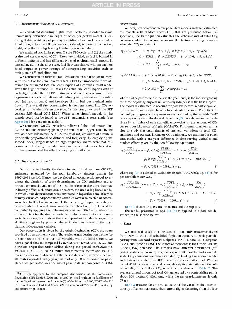
3.1. Measurement of aviation CO2 emissions

We considered departing flights from Lombardy in order to avoidunnecessary definition challenges of other perspectives—that is, en-tering flights, residency of passengers, airlines’ base, or kerosene sales.In addition, only direct flights were considered; in cases of connectingflight, only the first leg leaving Lombardy was included.

We analyzed two flight phases: (1) the LTO cycle; and (2) the climb,cruise and descent cycle (CCD). These are divided, as fuel is burned indifferent patterns and has different types of environmental impact. Inparticular, during the LTO cycle, fuel flow can change with an engine'srated output in power settings of corresponding activities such astaxing, take-off, and climb out.

We considered an aircraft's total emissions on a particular journey.With the aid of the small emitters tool (SET) by Eurocontrol,12 we ob-tained the estimated total fuel consumption of a certain aircraft modelgiven the flight distance. SET takes the actual fuel consumption data ofeach flight under the EU ETS initiative and then runs separate linearregressions of each aircraft model, defining two parameters: the inter-cept (at zero distance) and the slope (kg of fuel per nautical milesflown). The overall fuel consumption is then translated into CO2 ac-cording to the aircraft's engine type. In this study, we used the SETversion 5.05 dated 2015.12.26. When some aircraft models in thesample could not be found in the SET, assumptions were made (SeeAppendix I for conversion table.).

We computed two CO2 emissions indices: (1) the total amount and(2) the emission efficiency given by the amount of CO2 generated by theavailable seat kilometers (ASK). As the total CO2 emissions of a route isprincipally proportional to distance and frequency, by employing thesecond index, long-distance or high-frequency routes were not dis-criminated. Utilizing available seats in the second index formationfurther screened out the effect of varying aircraft sizes.

3.2. The econometric model

Our aim is to identify the determinants of total and per-ASK CO2

emissions generated by the four Lombardy airports during the1997–2011 period. Hence, we developed an econometric model to es-timate the elasticity of some determinants on CO2 emissions and toprovide empirical evidence of the possible effects of decisions that mayindirectly affect such emissions. Therefore, we used a log-linear modelin which some determinants were expressed in logarithms and others asdummy variables. Airport dummy variables were also created as controlvariables. In this log-linear model, the percentage impact on a depen-dent variable when a dummy variable switches from 0 to 1 could becomputed by applying the following expression: −e100( 1)δ , where δ isthe coefficient for the dummy variable. In the presence of a continuousvariable as a regressor, given that the dependent variable is logged, itselasticity is given by β —i.e., the estimated coefficient of the loga-rithmic independent variable.

Our observation is given by the origin-destination (OD), the routeprovided by an airline in year t. The triplet origin-destination-airline (orthe pair route-airline) is our “id” variable, with the label i. Hence wehave a panel data set composed by i = 1, 2, …., andI triplets origin-destination-airline during the period t = 1, 2, …, 15. Four hundred and thirty-five routes and 197 dif-ferent airlines were observed in the period data set; however, since notall routes operated every year, we had only 1082 route-airline pairs.Hence we generated an unbalanced panel data set composed of 4164

observations.We designed two econometric panel data models and then estimated

the models with random effects (RE) that are presented below (re-spectively, the first equation estimates the determinants of total CO2

emissions while the second concerns the factors affecting per-seat-kilometer CO2 emissions):

∑= + × + × + ×+ × + × + × + ×

+ × + × +=

CO α β logFUEL β logKM β SIZEβ TIME δ DEHUB δ δ LCC

δ EU γ D airport

log 2 log1998

_ ϵ

it t it it

t t t i

ij

j ij it

1 2 3

4 1 2 3

41

3

(1)

∑= + × + × + ×+ × + × + × + ×

+ × + × +=

CO ASK α β logFUEL β KM β SIZEβ TIME δ DEHUB δ δ LCC

δ EU γ airport

log 2 log log1998

ϵ

it t it it

t t t i

ii

i i it

1 2 3

4 1 2 3

41

3

(2)

where i is the pair route-airline, t is the year, and j is the index regardingthe three departing airports in Lombardy (Malpensa is the base airport).The model is estimated to account for possible heteroskedasticity—i.e.,the estimate coefficients have robust standard errors. The effect oftechnology progress on CO2 emissions is captured by the variable TIMEgiven by each year in the dataset. Equation (2) has a dependent variablegiven by an index of emission efficiency—that is, the amount of CO2

per-seat per kilometer of flight (CO2ASK). Furthermore, as our aim isalso to study the determinants of one-year variations in total CO2

emissions and per-seat-kilometer CO2 emissions, we estimated a paneldata model with a one-year difference in time-varying variables andrandom effects given by the two following equations:

= + × + ×+ × + × −+ × − +

− − −− −

−

COCO

α β log FUELFUEL

β log KMKM

β SIZESIZE

δ DEBUG DEBUG

δ υ

log( 22

) ( ) ( )

log( ) ( )

(1998 1998 )

it

it

t

t

it

it

it

itt t

t t it

11

12

1

31

1 1

2 1 (3)

where Eq. (3) is related to variations in total CO2, while Eq. (4) is forper-seat-kilometer CO2,

= + × + ×+ × + × −+ × − +

− − −− −

−

CO ASKCO ASK

α β log FUELFUEL

β log KMKM

β SIZESIZE

δ DEBUG DEBUG

δ υ

log( 22

) ( ) ( )

log( ) ( )

((1998 1998 ))

it

it

t

t

it

it

it

itt t

t t it

11

12

1

31

1 1

2 1 (4)

Table 1 illustrates the variable names and description.The model presented in Eqs. (1)–(4) is applied to a data set de-

scribed in the section below.

4. Data

We built a data set that included all Lombardy passenger flightsfrom 1997 to 2011, all scheduled flights in January of each year de-parting from Lombard airports: Malpensa (MXP), Linate (LIN), Bergamo(BGY), and Brescia (VBS). The source of these data is the Official AirlineGuide (OAG) database. The airports have different destination (air-ports), distances, carriers, frequencies, aircraft models, and availableseats. CO2 emissions are then estimated by feeding the aircraft modeland distance traveled into SET, the emission calculation tool. We col-lected 4197 observations and some descriptive statistics on the ob-served flights, and their CO2 emissions are shown in Table 2. Theaverage, annual amount of total CO2 generated by a route-airline pair isabout 800 thousand kilograms, while the per-seat-kilometers is only97 g+

Table 3 presents descriptive statistics of the variables that may in-directly affect emissions and the share of flights departing from the four

12 SET was approved by the European Commission via the CommissionRegulation (EU) No.606/2010 and is used by small emitters in fulfillment oftheir obligations pursuant to Article 14(3) of the Directive 2003/87/EC (the EUETS Directive) and Part 4 of Annex XIV to Decision 2007/589/EC (monitoringand reporting guidance).


�

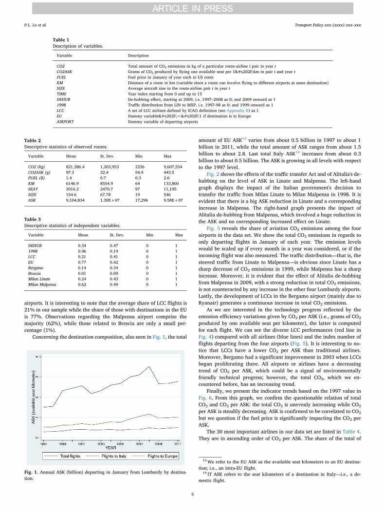
airports. It is interesting to note that the average share of LCC flights is21% in our sample while the share of those with destinations in the EUis 77%. Observations regarding the Malpensa airport comprise themajority (62%), while those related to Brescia are only a small per-centage (1%).

Concerning the destination composition, also seen in Fig. 1, the total

amount of EU ASK13 varies from about 0.5 billion in 1997 to about 1billion in 2011, while the total amount of ASK ranges from about 1.5billion to about 2.8. Last total Italy ASK14 increases from about 0.3billion to about 0.5 billion. The ASK is growing in all levels with respectto the 1997 level.

Fig. 2 shows the effects of the traffic transfer Act and of Alitalia's de-hubbing on the level of ASK in Linate and Malpensa. The left-handgraph displays the impact of the Italian government's decision totransfer the traffic from Milan Linate to Milan Malpensa in 1998. It isevident that there is a big ASK reduction in Linate and a correspondingincrease in Malpensa. The right-hand graph presents the impact ofAlitalia de-hubbing from Malpensa, which involved a huge reduction inthe ASK and no corresponding increased effect on Linate.

Fig. 3 reveals the share of aviation CO2 emissions among the fourairports in the data set. We show the total CO2 emissions in regards toonly departing flights in January of each year. The emission levelswould be scaled up if every month in a year was considered, or if theincoming flight was also measured. The traffic distribution—that is, thesteered traffic from Linate to Malpensa—is obvious since Linate has asharp decrease of CO2 emissions in 1999, while Malpensa has a sharpincrease. Moreover, it is evident that the effect of Alitalia de-hubbingfrom Malpensa in 2009, with a strong reduction in total CO2 emissions,is not counteracted by any increase in the other four Lombardy airports.Lastly, the development of LCCs in the Bergamo airport (mainly due toRyanair) generates a continuous increase in total CO2 emissions.

As we are interested in the technology progress reflected by theemission efficiency variations given by CO2 per ASK (i.e., grams of CO2

produced by one available seat per kilometer), the latter is computedfor each flight. We can see the diverse LCC performances (red line inFig. 4) compared with all airlines (blue lines) and the index number offlights departing from the four airports (Fig. 5). It is interesting to no-tice that LCCs have a lower CO2 per ASK than traditional airlines.Moreover, Bergamo had a significant improvement in 2003 when LCCsbegan proliferating there. All airports or airlines have a decreasingtrend of CO2 per ASK, which could be a signal of environmentallyfriendly technical progress; however, the total CO2, which we en-countered before, has an increasing trend.

Finally, we present the indicator trends based on the 1997 value inFig. 6. From this graph, we confirm the questionable relation of totalCO2 and CO2 per ASK: the total CO2 is unevenly increasing while CO2

per ASK is steadily decreasing. ASK is confirmed to be correlated to CO2

but we question if the fuel price is significantly impacting the CO2 perASK.

The 30 most important airlines in our data set are listed in Table 4.They are in ascending order of CO2 per ASK. The share of the total of

Table 1Description of variables.

Variable Description

CO2 Total amount of CO2 emissions in kg of a particular route-airline i pair in year tCO2ASK Grams of CO2 produced by flying one available seat per 1 km in pair i and year tFUEL Fuel price in January of year each in US centsKM Distance of a route in km (variable since a route can involve flying to different airports at same destination)SIZE Average aircraft size in the route-airline pair i in year tTIME Year index starting from 0 and up to 15DEHUB De-hubbing effect, starting at 2009, i.e. 1997–2008 as 0; and 2009 onward as 11998 Traffic distribution from LIN to MXP, i.e. 1997-98 as 0; and 1999 onward as 1LCC A set of LCC airlines defined by ICAO definition (see Appendix II) as 1EU Dummy variable = 1 if destination is in EuropeAIRPORT Dummy variable of departing airports

Table 2Descriptive statistics of observed routes.

Variable Mean St. Dev. Min Max

CO2 (kg) 821,386.4 1,203,953 2236 9,607,554CO2ASK (g) 97.3 32.4 54.9 443.5FUEL ($) 1.4 0.7 0.3 2.6KM 6146.9 8554.9 64 133,800SEAT 2016.2 2470.7 97 11,195SIZE 154.6 67.78 19 546ASK 9,104,834 1.30E+07 17,296 9.58E+07

Table 3Descriptive statistics of independent variables.

Variable Mean St. Dev. Min Max

DEHUB 0.34 0.47 0 11998 0.96 0.19 0 1LCC 0.21 0.41 0 1EU 0.77 0.42 0 1Bergamo 0.14 0.34 0 1Brescia 0.01 0.09 0 1Milan Linate 0.24 0.43 0 1Milan Malpensa 0.62 0.49 0 1

Fig. 1. Annual ASK (billion) departing in January from Lombardy by destina-tion.

13 We refer to the EU ASK as the available seat kilometers to an EU destina-tion; i.e., an intra-EU flight.

14 IT ASK refers to the seat kilometers of a destination in Italy—i.e., a do-mestic flight.


�

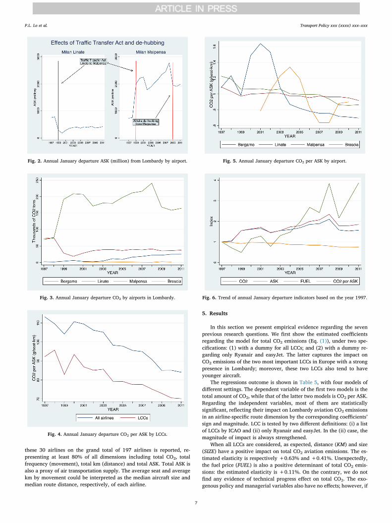
these 30 airlines on the grand total of 197 airlines is reported, re-presenting at least 80% of all dimensions including total CO2, totalfrequency (movement), total km (distance) and total ASK. Total ASK isalso a proxy of air transportation supply. The average seat and averagekm by movement could be interpreted as the median aircraft size andmedian route distance, respectively, of each airline.

5. Results

In this section we present empirical evidence regarding the sevenprevious research questions. We first show the estimated coefficientsregarding the model for total CO2 emissions (Eq. (1)), under two spe-cifications: (1) with a dummy for all LCCs; and (2) with a dummy re-garding only Ryanair and easyJet. The latter captures the impact onCO2 emissions of the two most important LCCs in Europe with a strongpresence in Lombardy; moreover, these two LCCs also tend to haveyounger aircraft.

The regressions outcome is shown in Table 5, with four models ofdifferent settings. The dependent variable of the first two models is thetotal amount of CO2, while that of the latter two models is CO2 per ASK.Regarding the independent variables, most of them are statisticallysignificant, reflecting their impact on Lombardy aviation CO2 emissionsin an airline-specific route dimension by the corresponding coefficients’sign and magnitude. LCC is tested by two different definitions: (i) a listof LCCs by ICAO and (ii) only Ryanair and easyJet. In the (ii) case, themagnitude of impact is always strengthened.

When all LCCs are considered, as expected, distance (KM) and size(SIZE) have a positive impact on total CO2 aviation emissions. The es-timated elasticity is respectively +0.63% and +0.41%. Unexpectedly,the fuel price (FUEL) is also a positive determinant of total CO2 emis-sions: the estimated elasticity is +0.11%. On the contrary, we do notfind any evidence of technical progress effect on total CO2. The exo-genous policy and managerial variables also have no effects; however, if

Fig. 2. Annual January departure ASK (million) from Lombardy by airport.

Fig. 3. Annual January departure CO2 by airports in Lombardy.

Fig. 4. Annual January departure CO2 per ASK by LCCs.

Fig. 5. Annual January departure CO2 per ASK by airport.

Fig. 6. Trend of annual January departure indicators based on the year 1997.


�

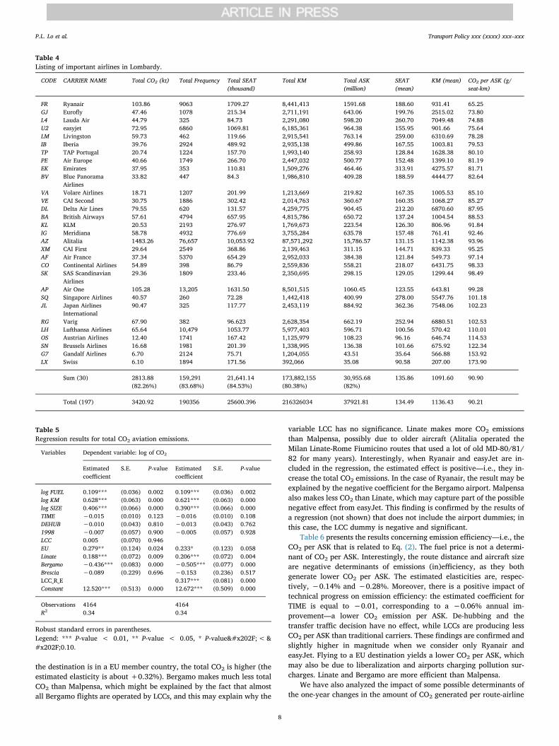
the destination is in a EU member country, the total CO2 is higher (theestimated elasticity is about +0.32%). Bergamo makes much less totalCO2 than Malpensa, which might be explained by the fact that almostall Bergamo flights are operated by LCCs, and this may explain why the

variable LCC has no significance. Linate makes more CO2 emissionsthan Malpensa, possibly due to older aircraft (Alitalia operated theMilan Linate-Rome Fiumicino routes that used a lot of old MD-80/81/82 for many years). Interestingly, when Ryanair and easyJet are in-cluded in the regression, the estimated effect is positive—i.e., they in-crease the total CO2 emissions. In the case of Ryanair, the result may beexplained by the negative coefficient for the Bergamo airport. Malpensaalso makes less CO2 than Linate, which may capture part of the possiblenegative effect from easyJet. This finding is confirmed by the results ofa regression (not shown) that does not include the airport dummies; inthis case, the LCC dummy is negative and significant.

Table 6 presents the results concerning emission efficiency—i.e., theCO2 per ASK that is related to Eq. (2). The fuel price is not a determi-nant of CO2 per ASK. Interestingly, the route distance and aircraft sizeare negative determinants of emissions (in)efficiency, as they bothgenerate lower CO2 per ASK. The estimated elasticities are, respec-tively, −0.14% and −0.28%. Moreover, there is a positive impact oftechnical progress on emission efficiency: the estimated coefficient forTIME is equal to −0.01, corresponding to a −0.06% annual im-provement—a lower CO2 emission per ASK. De-hubbing and thetransfer traffic decision have no effect, while LCCs are producing lessCO2 per ASK than traditional carriers. These findings are confirmed andslightly higher in magnitude when we consider only Ryanair andeasyJet. Flying to a EU destination yields a lower CO2 per ASK, whichmay also be due to liberalization and airports charging pollution sur-charges. Linate and Bergamo are more efficient than Malpensa.

We have also analyzed the impact of some possible determinants ofthe one-year changes in the amount of CO2 generated per route-airline

Table 4Listing of important airlines in Lombardy.

CODE CARRIER NAME Total CO2 (kt) Total Frequency Total SEAT(thousand)

Total KM Total ASK(million)

SEAT(mean)

KM (mean) CO2 per ASK (g/seat-km)

FR Ryanair 103.86 9063 1709.27 8,441,413 1591.68 188.60 931.41 65.25GJ Eurofly 47.46 1078 215.34 2,711,191 643.06 199.76 2515.02 73.80L4 Lauda Air 44.79 325 84.73 2,291,080 598.20 260.70 7049.48 74.88U2 easyjet 72.95 6860 1069.81 6,185,361 964.38 155.95 901.66 75.64LM Livingston 59.73 462 119.66 2,915,541 763.14 259.00 6310.69 78.28IB Iberia 39.76 2924 489.92 2,935,138 499.86 167.55 1003.81 79.53TP TAP Portugal 20.74 1224 157.70 1,993,140 258.93 128.84 1628.38 80.10PE Air Europe 40.66 1749 266.70 2,447,032 500.77 152.48 1399.10 81.19EK Emirates 37.95 353 110.81 1,509,276 464.46 313.91 4275.57 81.71BV Blue Panorama

Airlines33.82 447 84.3 1,986,810 409.28 188.59 4444.77 82.64

VA Volare Airlines 18.71 1207 201.99 1,213,669 219.82 167.35 1005.53 85.10VE CAI Second 30.75 1886 302.42 2,014,763 360.67 160.35 1068.27 85.27DL Delta Air Lines 79.55 620 131.57 4,259,775 904.45 212.20 6870.60 87.95BA British Airways 57.61 4794 657.95 4,815,786 650.72 137.24 1004.54 88.53KL KLM 20.53 2193 276.97 1,769,673 223.54 126.30 806.96 91.84IG Meridiana 58.78 4932 776.69 3,755,284 635.78 157.48 761.41 92.46AZ Alitalia 1483.26 76,657 10,053.92 87,571,292 15,786.57 131.15 1142.38 93.96XM CAI First 29.64 2549 368.86 2,139,463 311.15 144.71 839.33 95.25AF Air France 37.34 5370 654.29 2,952,033 384.38 121.84 549.73 97.14CO Continental Airlines 54.89 398 86.79 2,559,836 558.21 218.07 6431.75 98.33SK SAS Scandinavian

Airlines29.36 1809 233.46 2,350,695 298.15 129.05 1299.44 98.49

AP Air One 105.28 13,205 1631.50 8,501,515 1060.45 123.55 643.81 99.28SQ Singapore Airlines 40.57 260 72.28 1,442,418 400.99 278.00 5547.76 101.18JL Japan Airlines

International90.47 325 117.77 2,453,119 884.92 362.36 7548.06 102.23

RG Varig 67.90 382 96.623 2,628,354 662.19 252.94 6880.51 102.53LH Lufthansa Airlines 65.64 10,479 1053.77 5,977,403 596.71 100.56 570.42 110.01OS Austrian Airlines 12.40 1741 167.42 1,125,979 108.23 96.16 646.74 114.53SN Brussels Airlines 16.68 1981 201.39 1,338,995 136.38 101.66 675.92 122.34G7 Gandalf Airlines 6.70 2124 75.71 1,204,055 43.51 35.64 566.88 153.92LX Swiss 6.10 1894 171.56 392,066 35.08 90.58 207.00 173.90

Sum (30) 2813.88(82.26%)

159,291(83.68%)

21,641.14(84.53%)

173,882,155(80.38%)

30,955.68(82%)

135.86 1091.60 90.90

Total (197) 3420.92 190356 25600.396 216326034 37921.81 134.49 1136.43 90.21

Table 5Regression results for total CO2 aviation emissions.

Variables Dependent variable: log of CO2

Estimatedcoefficient

S.E. P-value Estimatedcoefficient

S.E. P-value

log FUEL 0.109*** (0.036) 0.002 0.109*** (0.036) 0.002log KM 0.628*** (0.063) 0.000 0.621*** (0.063) 0.000log SIZE 0.406*** (0.066) 0.000 0.390*** (0.066) 0.000TIME −0.015 (0.010) 0.123 −0.016 (0.010) 0.108DEHUB −0.010 (0.043) 0.810 −0.013 (0.043) 0.7621998 −0.007 (0.057) 0.900 −0.005 (0.057) 0.928LCC 0.005 (0.070) 0.946EU 0.279** (0.124) 0.024 0.233* (0.123) 0.058Linate 0.188*** (0.072) 0.009 0.206*** (0.072) 0.004Bergamo −0.436*** (0.083) 0.000 −0.505*** (0.077) 0.000Brescia −0.089 (0.229) 0.696 −0.153 (0.236) 0.517LCC_R_E 0.317*** (0.081) 0.000Constant 12.520*** (0.513) 0.000 12.672*** (0.509) 0.000

Observations 4164 4164R2 0.34 0.34

Robust standard errors in parentheses.Legend: *** P-value < 0.01, ** P-value < 0.05, * P-value < 0.10.


�

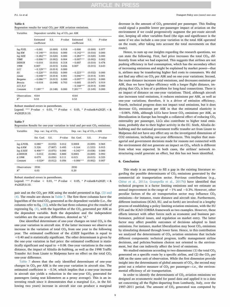
pair and on the CO2 per ASK using the model presented in Eqs. (3) and(4). The results are shown in Table 7. The first three columns have thelogarithm of the total CO2 generated as the dependent variable (i.e., thecolumns refer to Eq. (3)), while the last three columns give the results ofregressing Eq. (4), with the logarithm of the CO2 generated per ASK asthe dependent variable. Both the dependent and the independentvariables are the one-year difference, denoted as “d.”

One identified determinant of one-year changes on total CO2 is theone-year variation in aircraft size. If the latter increases we observe anincrease in the variation of total CO2 from one year to the followingyear. The estimated coefficient of the d.SIZE logarithm is equal to+0.40 and is statistically significant. The other determinant is given bythe one-year variation in fuel price: the estimated coefficient is statis-tically significant and equal to +0.08. One-year variations in the routedistance, the impact of Alitalia de-hubbing, as well as the 1998 TrafficTransfer Act from Linate to Malpensa have no effect on the total CO2

one-year difference.Table 7 shows that the only identified determinant of one-year

changes in CO2 per ASK is the one-year variation in aircraft size. Theestimated coefficient is −0.34, which implies that a one-year increasein aircraft size yields a reduction in the one-year CO2 generated forpassengers (using seat kilometers as a proxy average). This is an in-teresting result since it demonstrates that a marginal (i.e., in the fol-lowing two years) increase in aircraft size can produce a marginal

decrease in the amount of CO2 generated per passenger. This findingcould signal a possible lower per-passenger impact of aviation on theenvironment if we could progressively augment the per-route aircraftsize, keeping all other variables fixed (the sign and significance is thesame if we also include a one-year variation in the total ASK operatedon the route, after taking into account the total movements on thatroute).

Hence, to sum up our insights regarding the research questions, wecan state the following. First, fuel price increases the total CO2, dif-ferently from what we had expected. This suggests that airlines are notpushing efficiency in fuel consumption, which has the secondary effectof increasing emissions and might be explained by market power—thatis, airlines may be transferring higher fuel costs to consumers. We didnot find any effect on CO2 per ASK and on one-year variations. Second,the route distance increases total emissions, and decreases emission perASK, thus we have higher efficiency with a longer flight distance, im-plying that CO2 is less of a problem for long-haul connections. There isno impact of distance on one-year variations. Third, although aircraftsize increases total emissions, it reduces emissions per ASK, as well asone-year variations; therefore, it is a driver of emission efficiency.Fourth, technical progress does not impact total emissions, but it doesdecrease CO2 emissions per ASK in that the estimated elasticity is−0.06%. Fifth, although LCCs have lower CO2 emissions per ASK, asliberalization in Europe has brought a collateral effect of reducing CO2

externality per passenger, LLCs also contribute to higher total emis-sions, probably due to their higher activity in the EU. Sixth, Alitalia de-hubbing and the national government traffic transfer act from Linate toMalpensa did not have any effect any on the investigated dimensions ofCO2 emissions, including one-year differences. This implies that man-agerial and government decisions made for reasons not connected withthe environment did not generate an impact on CO2, which is differentfrom what was expected. In both cases, the airlines’ network re-structuring could generate an effect, but this has not been identified.

6. Conclusion

This study is an attempt to fill a gap in the existing literature re-garding the possible determinants of CO2 emissions generated by thecommercial air transportation sector. Previous contributions (e.g.,Chèze et al., 2011a; Grampella et al., 2017b) have identified thattechnical progress is a factor limiting emissions and we estimate anannual improvement in the range of −1% and −0.3%. However, otherpeculiar factors of the air transportation sector may influence CO2

emissions—for instance, route distance and aircraft size. Furthermore,different institutions (ICAO, EU, and so forth) are involved in a lengthyprocess of establishing a policy limiting aviation emissions, with the EUETS and the ICAO CORSIA framework as two examples. However, theseefforts interact with other forces such as economic and business per-formance, political issues, and regulation on market entry. The latterfactor may affect possible outcomes of decisions adopted to limitemissions. For instance, market liberalization may boost CO2 emissionsby stimulating demand through lower fares. Hence, in this contributionwe analyzed the determinants of CO2 aviation emissions that includedifferent components: technical progress, traffic management airlinedecisions, and policies/business choices not oriented to the environ-ment, but that can indirectly affect the level of emissions.

We studied emissions according to two dimensions: (1) the total CO2

generated on a specific route by a specific airline, and (2) the CO2 perASK on the same unit of observation. While the first dimension provideinsight into the determinants of global amounts of CO2, the second maypoint out a relative measure of CO2 per passenger—i.e., the environ-mental efficiency of air transportation.

In order to identify the determinants of CO2 aviation emissions wedesigned an econometric model for panel data and applied it to a dataset concerning all the flights departing from Lombardy, Italy, over the1997–2011 period. The amount of CO2 generated was computed by

Table 6Regression results for total CO2 per ASK aviation emissions.

Variables Dependent variable: log of CO2 per ASK

Estimatedcoefficient

S.E. P-value Estimatedcoefficient

S.E. P-value

log FUEL −0.001 (0.009) 0.918 −0.000 (0.009) 0.977log KM −0.140*** (0.016) 0.000 −0.142*** (0.016) 0.000log SIZE −0.282*** (0.020) 0.000 −0.283*** (0.020) 0.000TIME −0.006*** (0.002) 0.004 −0.007*** (0.002) 0.002DEHUB −0.010 (0.010) 0.318 −0.007 (0.010) 0.4781998 0.007 (0.015) 0.656 0.007 (0.015) 0.643LCC −0.129*** (0.014) 0.000EU −0.220*** (0.032) 0.000 −0.223*** (0.032) 0.000Linate −0.048*** (0.014) 0.001 −0.046*** (0.014) 0.001Bergamo −0.086*** (0.015) 0.000 −0.097*** (0.015) 0.000Brescia −0.018 (0.048) 0.703 −0.005 (0.047) 0.919LCC_R_E −0.168*** (0.014) 0.000Constant 7.189*** (0.148) 0.000 7.201*** (0.149) 0.000

Observations 4164 4164R2 0.53 0.53


Table 7Regression Results for one-year variation in total and per-seat CO2 emissions.

Variables Dep. var.: log of CO2 Dep. var.: log of CO2 x ASK

Est. Coef. S.E. P-value Est. Coef. S.E. P-value

log d.FUEL 0.080** (0.032) 0.012 0.0004 (0.009) 0.965log d.KM 5.326 (7.807) 0.495 −0.164 (1.533) 0.915log d.SIZE 0.400*** (0.075) 0.000 −0.342*** (0.038) 0.000d.DEHUB −0.012 (0.046) 0.800 0.0001 (0.009) 0.992d.1998 0.079 (0.050) 0.111 0.015 (0.015) 0.325Constant −0.024* (0.012) 0.056 −0.006*** (0.002) 0.007

Observations 2930 2930R2 0.03 0.20



�

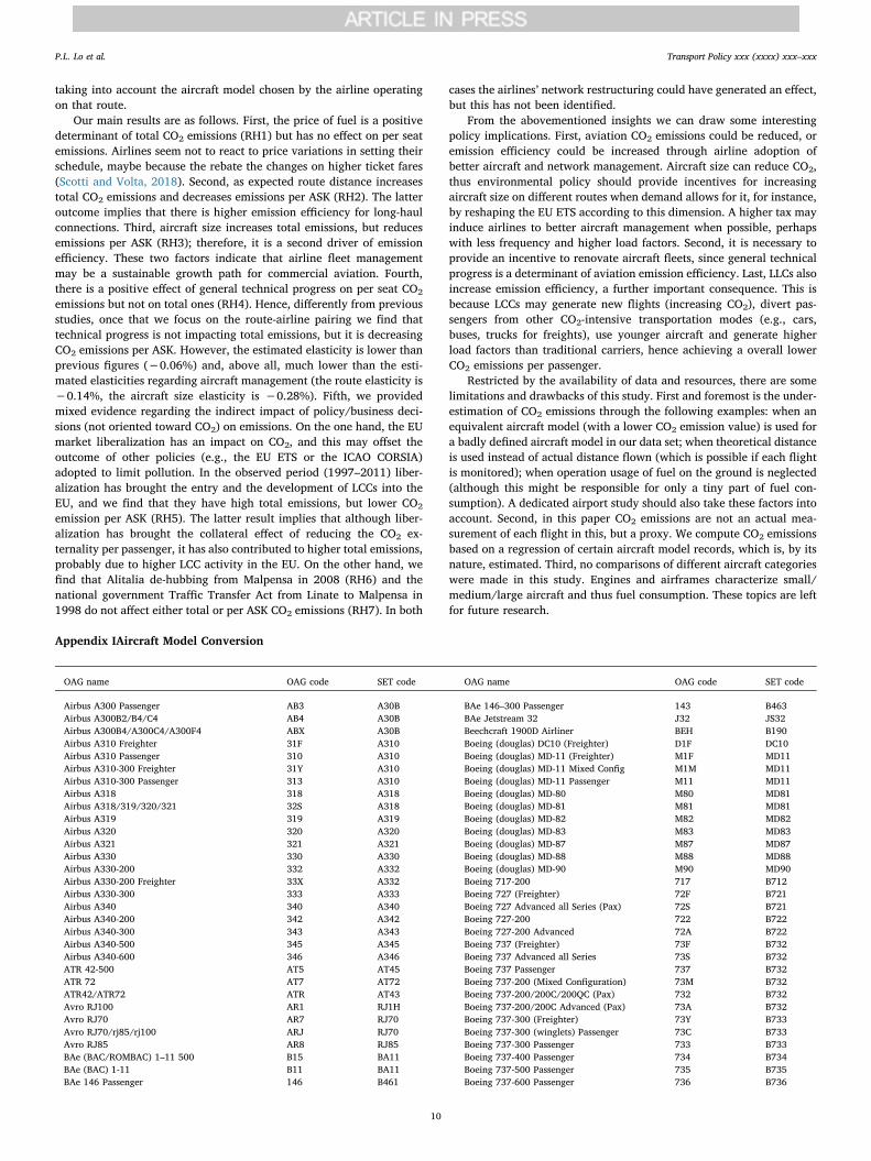
taking into account the aircraft model chosen by the airline operatingon that route.

Our main results are as follows. First, the price of fuel is a positivedeterminant of total CO2 emissions (RH1) but has no effect on per seatemissions. Airlines seem not to react to price variations in setting theirschedule, maybe because the rebate the changes on higher ticket fares(Scotti and Volta, 2018). Second, as expected route distance increasestotal CO2 emissions and decreases emissions per ASK (RH2). The latteroutcome implies that there is higher emission efficiency for long-haulconnections. Third, aircraft size increases total emissions, but reducesemissions per ASK (RH3); therefore, it is a second driver of emissionefficiency. These two factors indicate that airline fleet managementmay be a sustainable growth path for commercial aviation. Fourth,there is a positive effect of general technical progress on per seat CO2

emissions but not on total ones (RH4). Hence, differently from previousstudies, once that we focus on the route-airline pairing we find thattechnical progress is not impacting total emissions, but it is decreasingCO2 emissions per ASK. However, the estimated elasticity is lower thanprevious figures (−0.06%) and, above all, much lower than the esti-mated elasticities regarding aircraft management (the route elasticity is−0.14%, the aircraft size elasticity is −0.28%). Fifth, we providedmixed evidence regarding the indirect impact of policy/business deci-sions (not oriented toward CO2) on emissions. On the one hand, the EUmarket liberalization has an impact on CO2, and this may offset theoutcome of other policies (e.g., the EU ETS or the ICAO CORSIA)adopted to limit pollution. In the observed period (1997–2011) liber-alization has brought the entry and the development of LCCs into theEU, and we find that they have high total emissions, but lower CO2

emission per ASK (RH5). The latter result implies that although liber-alization has brought the collateral effect of reducing the CO2 ex-ternality per passenger, it has also contributed to higher total emissions,probably due to higher LCC activity in the EU. On the other hand, wefind that Alitalia de-hubbing from Malpensa in 2008 (RH6) and thenational government Traffic Transfer Act from Linate to Malpensa in1998 do not affect either total or per ASK CO2 emissions (RH7). In both

cases the airlines’ network restructuring could have generated an effect,but this has not been identified.

From the abovementioned insights we can draw some interestingpolicy implications. First, aviation CO2 emissions could be reduced, oremission efficiency could be increased through airline adoption ofbetter aircraft and network management. Aircraft size can reduce CO2,thus environmental policy should provide incentives for increasingaircraft size on different routes when demand allows for it, for instance,by reshaping the EU ETS according to this dimension. A higher tax mayinduce airlines to better aircraft management when possible, perhapswith less frequency and higher load factors. Second, it is necessary toprovide an incentive to renovate aircraft fleets, since general technicalprogress is a determinant of aviation emission efficiency. Last, LLCs alsoincrease emission efficiency, a further important consequence. This isbecause LCCs may generate new flights (increasing CO2), divert pas-sengers from other CO2-intensive transportation modes (e.g., cars,buses, trucks for freights), use younger aircraft and generate higherload factors than traditional carriers, hence achieving a overall lowerCO2 emissions per passenger.

Restricted by the availability of data and resources, there are somelimitations and drawbacks of this study. First and foremost is the under-estimation of CO2 emissions through the following examples: when anequivalent aircraft model (with a lower CO2 emission value) is used fora badly defined aircraft model in our data set; when theoretical distanceis used instead of actual distance flown (which is possible if each flightis monitored); when operation usage of fuel on the ground is neglected(although this might be responsible for only a tiny part of fuel con-sumption). A dedicated airport study should also take these factors intoaccount. Second, in this paper CO2 emissions are not an actual mea-surement of each flight in this, but a proxy. We compute CO2 emissionsbased on a regression of certain aircraft model records, which is, by itsnature, estimated. Third, no comparisons of different aircraft categorieswere made in this study. Engines and airframes characterize small/medium/large aircraft and thus fuel consumption. These topics are leftfor future research.

Appendix IAircraft Model Conversion

OAG name OAG code SET code OAG name OAG code SET code

Airbus A300 Passenger AB3 A30B BAe 146–300 Passenger 143 B463Airbus A300B2/B4/C4 AB4 A30B BAe Jetstream 32 J32 JS32Airbus A300B4/A300C4/A300F4 ABX A30B Beechcraft 1900D Airliner BEH B190Airbus A310 Freighter 31F A310 Boeing (douglas) DC10 (Freighter) D1F DC10Airbus A310 Passenger 310 A310 Boeing (douglas) MD-11 (Freighter) M1F MD11Airbus A310-300 Freighter 31Y A310 Boeing (douglas) MD-11 Mixed Config M1M MD11Airbus A310-300 Passenger 313 A310 Boeing (douglas) MD-11 Passenger M11 MD11Airbus A318 318 A318 Boeing (douglas) MD-80 M80 MD81Airbus A318/319/320/321 32S A318 Boeing (douglas) MD-81 M81 MD81Airbus A319 319 A319 Boeing (douglas) MD-82 M82 MD82Airbus A320 320 A320 Boeing (douglas) MD-83 M83 MD83Airbus A321 321 A321 Boeing (douglas) MD-87 M87 MD87Airbus A330 330 A330 Boeing (douglas) MD-88 M88 MD88Airbus A330-200 332 A332 Boeing (douglas) MD-90 M90 MD90Airbus A330-200 Freighter 33X A332 Boeing 717-200 717 B712Airbus A330-300 333 A333 Boeing 727 (Freighter) 72F B721Airbus A340 340 A340 Boeing 727 Advanced all Series (Pax) 72S B721Airbus A340-200 342 A342 Boeing 727-200 722 B722Airbus A340-300 343 A343 Boeing 727-200 Advanced 72A B722Airbus A340-500 345 A345 Boeing 737 (Freighter) 73F B732Airbus A340-600 346 A346 Boeing 737 Advanced all Series 73S B732ATR 42-500 AT5 AT45 Boeing 737 Passenger 737 B732ATR 72 AT7 AT72 Boeing 737-200 (Mixed Configuration) 73M B732ATR42/ATR72 ATR AT43 Boeing 737-200/200C/200QC (Pax) 732 B732Avro RJ100 AR1 RJ1H Boeing 737-200/200C Advanced (Pax) 73A B732Avro RJ70 AR7 RJ70 Boeing 737-300 (Freighter) 73Y B733Avro RJ70/rj85/rj100 ARJ RJ70 Boeing 737-300 (winglets) Passenger 73C B733Avro RJ85 AR8 RJ85 Boeing 737-300 Passenger 733 B733BAe (BAC/ROMBAC) 1–11 500 B15 BA11 Boeing 737-400 Passenger 734 B734BAe (BAC) 1-11 B11 BA11 Boeing 737-500 Passenger 735 B735BAe 146 Passenger 146 B461 Boeing 737-600 Passenger 736 B736


��

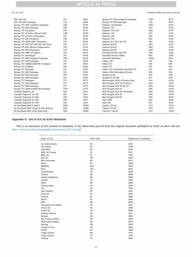
BAe 146-100 141 B461 Boeing 737-700 (winglets) Passenger 73W B737BAe 146–200 Passenger 142 B462 Boeing 737-700 Passenger 73G B737Boeing 737–800 (winglets) Passenger 73H B738 Embraer 120 Brasilia EM2 E120Boeing 737–800 Passenger 738 B738 Embraer 170 E70 E170Boeing 747 (Freighter) 74F B741 Embraer 170/195 EMJ E170Boeing 747 all Series (Mixed Conf) 74M B74D Embraer 175 E75 E170Boeing 747 all Series (Passenger) 747 B74D Embraer 190 E90 E190Boeing 747-200 (Freighter) 74X B742 Embraer 195 E95 E190Boeing 747–200B/200C (Passenger) 742 B742 Embraer RJ 135/140/145 ERJ E135Boeing 747-300/747-100/200 Sud (Pax) 743 B741 Embraer RJ135 ER3 E135Boeing 747-400 (Mixed Configuration) 74E B744 Embraer RJ145 ER4 E145Boeing 747-400 (Passenger) 744 B744 Embraer RJ145 EM4 E145Boeing 747–400F (Freighter) 74Y B744 Fairchild Dornier 328-100 D38 J328Boeing 757 (Passenger) 757 B752 Fairchild Dornier 328jet FRJ J328Boeing 757-200 (winglets) Passenger 75W B752 Fairchild Metroliner SWM SW4Boeing 757–200 Passenger 752 B752 Fokker 100 100 F28Boeing 757–200 PF (Freighter) 75F B752 Fokker 50 F50 F50Boeing 767 Freighter 76F B762 Fokker 70 F70 F70Boeing 767 Passenger 767 B762 Fokker F27 Friendship/Fairchild F27 F27 F27Boeing 767–200 Passenger 762 B762 Fokker F28 Fellowship all Series F28 F28Boeing 767–300 Passenger 763 B763 Ilyushin IL-86 ILW IL86Boeing 767–400 Passenger 764 B764 Ilyushin IL-96-300 IL9 IL96Boeing 777 Passenger 777 B772 McD-Douglas DC10 all Series (Pax) D10 DC10Boeing 777–200 Passenger 772 B772 McD-Douglas DC9 10/20 Series DC9 DC91Boeing 777–300 Passenger 773 B773 McD-Douglas DC9 30/40/50 D9S DC93Boeing 777–300 ER Passenger 77W B773 McD-Douglas DC9-20 D92 DC92Canadair Regional Jet CRJ CRJ1 McD-Douglas DC9-30 (Passenger) D93 DC93Canadair Regional Jet 100 CR1 CRJ1 McD-Douglas DC9-40 D94 DC93Canadair Regional Jet 200 CR2 CRJ2 McD-Douglas DC9-50 D95 DC95Canadair Regional Jet 700 CR7 CRJ7 Saab 2000 S20 SB20Canadair Regional Jet 900 CR9 CRJ9 Saab 340 SF3 SF34De Havilland DHC-8 Dash 8 DH8 DH8A Tupolev TU134 TU3 T134De Havilland DHC-8 Dash 8–400 Dash 8q DH4 DH8D Tupolev TU154 TU5 T154De Havilland DHC-8-300 Dash 8/8q DH3 DH8C Yakovlev Yak-40 YK4 YK40

Appendix II. List of LCC by ICAO Definition

This is an extraction of LCC present in Lombardy in the observation period from the original document published by ICAO on their web sitehttp://www.icao.int/sustainability/Documents/LCC-List.pdf.

Name of LCC IATA Code Registered in Lombardy

Air Arabia Maroc 3O 2010Air Europe PE 1999Atlas Blue 8A 2007Belle Air Europe L9 2011Belle Air LZ 2007Blue Air OB 2008Blue Panorama BV 2011Blue1 KF 2008BMIBaby WW 2003Buzz UK1 2001Centralwings CO 2006Clickair XG 2008Condor Flugdienst DE 2000easyJet U2 2004Flybe BE 2008Germanwings 4U 2003GO GO 1999ItAli Airlines 9X 2007Jet2.com LS 2004Jet4you 8J 2008MyAir 8I 2006Niki HG 2009Norwegian Air Shuttle DY 2011Ocean Air VC 2006Ocean Air 7VC 2006Pegasus Airlines H9 2011Ryanair FR 2001Sky Europe Airlines NE 2003SkyEurope Hungary 5P 2004Sterling NB 2003Transavia.com HV 2002TUIFly X3 2008Virgin Express BQ 1997Virgin Express TV 1997Vueling VY 2005


��

http://www.icao.int/sustainability/Documents/LCC-List.pdf

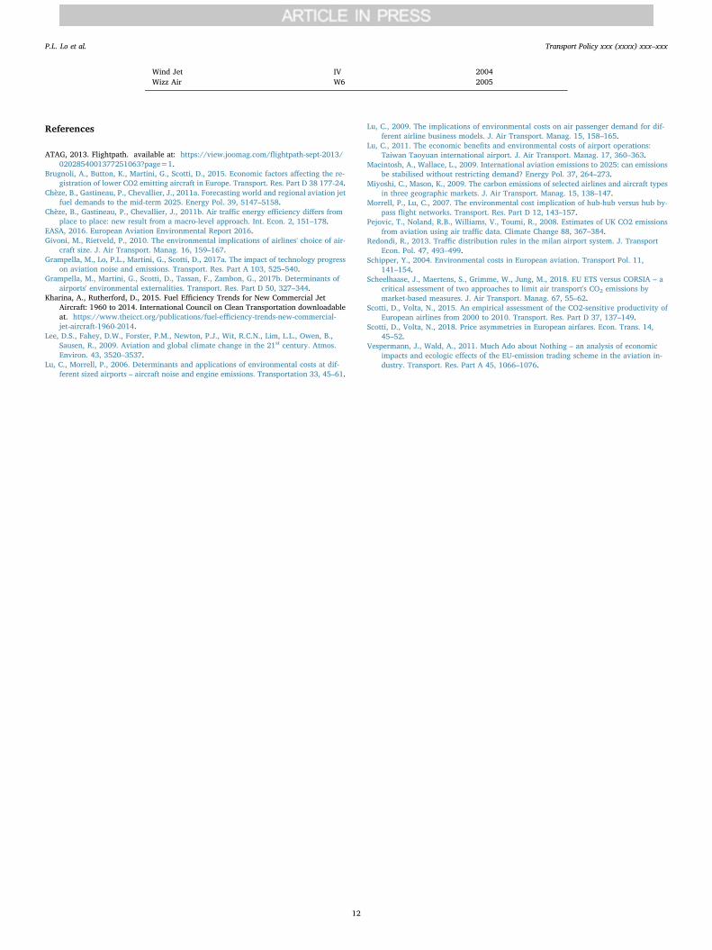
Wind Jet IV 2004Wizz Air W6 2005

References

ATAG, 2013. Flightpath. available at: https://view.joomag.com/flightpath-sept-2013/0202854001377251063?page=1.

Brugnoli, A., Button, K., Martini, G., Scotti, D., 2015. Economic factors affecting the re-gistration of lower CO2 emitting aircraft in Europe. Transport. Res. Part D 38 177-24.

Chèze, B., Gastineau, P., Chevallier, J., 2011a. Forecasting world and regional aviation jetfuel demands to the mid-term 2025. Energy Pol. 39, 5147–5158.

Chèze, B., Gastineau, P., Chevallier, J., 2011b. Air traffic energy efficiency differs fromplace to place: new result from a macro-level approach. Int. Econ. 2, 151–178.

EASA, 2016. European Aviation Environmental Report 2016.Givoni, M., Rietveld, P., 2010. The environmental implications of airlines' choice of air-

craft size. J. Air Transport. Manag. 16, 159–167.Grampella, M., Lo, P.L., Martini, G., Scotti, D., 2017a. The impact of technology progress

on aviation noise and emissions. Transport. Res. Part A 103, 525–540.Grampella, M., Martini, G., Scotti, D., Tassan, F., Zambon, G., 2017b. Determinants of

airports' environmental externalities. Transport. Res. Part D 50, 327–344.Kharina, A., Rutherford, D., 2015. Fuel Efficiency Trends for New Commercial Jet

Aircraft: 1960 to 2014. International Council on Clean Transportation downloadableat. https://www.theicct.org/publications/fuel-efficiency-trends-new-commercial-jet-aircraft-1960-2014.

Lee, D.S., Fahey, D.W., Forster, P.M., Newton, P.J., Wit, R.C.N., Lim, L.L., Owen, B.,Sausen, R., 2009. Aviation and global climate change in the 21st century. Atmos.Environ. 43, 3520–3537.

Lu, C., Morrell, P., 2006. Determinants and applications of environmental costs at dif-ferent sized airports – aircraft noise and engine emissions. Transportation 33, 45–61.

Lu, C., 2009. The implications of environmental costs on air passenger demand for dif-ferent airline business models. J. Air Transport. Manag. 15, 158–165.

Lu, C., 2011. The economic benefits and environmental costs of airport operations:Taiwan Taoyuan international airport. J. Air Transport. Manag. 17, 360–363.

Macintosh, A., Wallace, L., 2009. International aviation emissions to 2025: can emissionsbe stabilised without restricting demand? Energy Pol. 37, 264–273.

Miyoshi, C., Mason, K., 2009. The carbon emissions of selected airlines and aircraft typesin three geographic markets. J. Air Transport. Manag. 15, 138–147.

Morrell, P., Lu, C., 2007. The environmental cost implication of hub-hub versus hub by-pass flight networks. Transport. Res. Part D 12, 143–157.

Pejovic, T., Noland, R.B., Williams, V., Toumi, R., 2008. Estimates of UK CO2 emissionsfrom aviation using air traffic data. Climate Change 88, 367–384.

Redondi, R., 2013. Traffic distribution rules in the milan airport system. J. TransportEcon. Pol. 47, 493–499.

Schipper, Y., 2004. Environmental costs in European aviation. Transport Pol. 11,141–154.

Scheelhaase, J., Maertens, S., Grimme, W., Jung, M., 2018. EU ETS versus CORSIA – acritical assessment of two approaches to limit air transport's CO2 emissions bymarket-based measures. J. Air Transport. Manag. 67, 55–62.

Scotti, D., Volta, N., 2015. An empirical assessment of the CO2-sensitive productivity ofEuropean airlines from 2000 to 2010. Transport. Res. Part D 37, 137–149.

Scotti, D., Volta, N., 2018. Price asymmetries in European airfares. Econ. Trans. 14,45–52.

Vespermann, J., Wald, A., 2011. Much Ado about Nothing – an analysis of economicimpacts and ecologic effects of the EU-emission trading scheme in the aviation in-dustry. Transport. Res. Part A 45, 1066–1076.


��

https://view.joomag.com/flightpath-sept-2013/0202854001377251063?page=1

https://view.joomag.com/flightpath-sept-2013/0202854001377251063?page=1

http://refhub.elsevier.com/S0967-070X(17)30472-9/sref2













https://www.theicct.org/publications/fuel-efficiency-trends-new-commercial-jet-aircraft-1960-2014

https://www.theicct.org/publications/fuel-efficiency-trends-new-commercial-jet-aircraft-1960-2014
































Econometric Approach to Reveal Determinants of Air Cargo Volume of European Countries

Abstract GDP has long been used as an indicator of air cargo level as they both reflect international trading activity from different angles. This was true and proofed when international trading was mainly composed by manufacturing outcome. However, in the era of new economy, characterized by just in time manufacturing and express e-commerce, while GDP is weighting more on service industries, the indicator of air cargo should be verified. This paper explores alternative economic measurements of a country, which may be possibly related to its air cargo volume. Data of European countries from 2007 to 2015 are collected. After testing some hypothesis with a set of econometric model, we found that a country’s income level, online purchase activity and air cargo connectivity are all positive determinants of its air cargo level. We also draw some policy implications in the conclusion according to the findings and our understanding of transport and economics.

1. Introduction

Transport, as a channel to move people and goods, is vital to an economy (Brugnoli et al.

2018). In 2016, air transport supported 12.2 million jobs and $823 billion in European

economic activity, which are expected to grow at 3.4% per year (ATAG1, 2018). In the era

of e-commerce and just-in-time manufacturing, high value international trading and global

manufacturing were possibly initiated and developed wherever markets can be easily

connected frequently and quickly. The benefit for air transportation to tourist flow is well-

studied, given the determinants of air passengers’ movement and its effect on the local

economies; little is still instead known about the factors affecting air cargo activities, i.e., the

volume of goods that are shipped by air transport.

Air cargo revenue to an airport can be great enough to sustain a city. Memphis in the US is

among the most extreme cases, having over 4 billion pounds of cargo enplaned in 2004

resulting in $10 billion of associated revenue2. The economic value of air cargo was not fully

investigated despite of ICAO (2015) stressing that “air cargo services are a tremendous

enabler for economic progress in developing countries…”3. Only 38% cost-benefit analysis

1 Air Transport Action Group publish biennale report highlighting the industry outlook. 2 Sparks Bureau of Business and Economic Research (2005) measured the benefits resulted from aviation related activities at Memphis International Airport. 3 ICAO, International Civil Aviation Organization, highlighted the benefit to employment and economic growth by trading of electrical components, perishable products (food and flowers).

2

of airport, summarized by TRB4 (2009), quantified cargo benefit, the rest regarded such

benefit hard-to-quantify or side-product of passenger transport.

Comparing to measureable benefit generated by tourist, air cargo’s contribution was not

properly captured perhaps due to its complex nature and less obvious relationship with other

activities in the aviation business. Firstly, the beneficiaries may not be restricted to airlines,

airport or forwarder, but also manufacturers demanding reliable transport or consumers

enjoying the express services. Evidence of economic benefit of air cargo was shown in CBA

of Rock County Airport by Wisconsin DOT (2000)5, where the potential losses of

surrounding business during supply chain interruption is considered. Secondly, air freight has

low volume share among all mode of freight transport. However, the value of goods transport

by air is significantly important, especially to today’s new economies. Button (2000) proofed

the impact on new economy employment of international air service. These are values

beyond the yield of airports, carriers or integrators. Feng et al. (2015) summarized the main

differences between air cargo and air passenger business as uncertainty (changing in booking

or reservation in cargo business is very common), complexity (capacity forecast consists of

parameter such as pivot weight, pivot volume, and center of gravity) and flexibility (air cargo

can be transshipped more than one stop as long as it meets the delivery time). These could

explain the challenge in capturing the practical reality of air cargo business.

In 2014, as shown by Shepherd et al. (2016), 50 million tons of freight were carried by air

accounting only for 1% by volume but 35% of values of world traded goods. There is a very

wide range of goods favorable to air cargo, from fresh seafood and flowers to high value

electronics and hazard chemicals. Therefore, there are specific handling requirement and thus

specific players in the field. The boundaries between different category of service providers

is blurring when integration and cooperation becoming more common, some extreme cases

are express air cargo carrier providing extra door to door service in partnership or Amazon’s

prime air in turn providing air cargo service when there is extra capacity from their core

business.

4 Transportation Research Board, a division of the National Research Council of the United States. 5 The airport analyse the constrained runway impact on cargo activity. The expansion was finally approved when economic efficiency of cargo was considered on top of transportation cost saving. It shows that potential economic efficiency of cargo accounts for 40 million USD of labour costs and revenue losses due to production slowdown. Potential job losses are also highlighted when production shutdown, shifting 23,000 workplaces to other regions or countries.

3

This paper is aiming at finding out some determinants of air cargo traffic at the country level,

and at drawing some policy implications to airport or airline managers and governments,

when a strategy will be needed to boost air cargo traffic, or where will be the right place to

exploit air cargo traffic opportunities. We try to address these issues by building a data set

regarding European countries (EU28 + Switzerland + Iceland) during the period of 2007-15

and by designing a set of econometric model where possible determinants of air cargo levels

are investigated. We used different econometric methods to verify the robustness of the

model. We focus on some determinants that may explain the cargo levels in European

countries, e.g., the e-commerce activity, the country’s air cargo connectivity and the

country’s income.

We show that, one percentage point growth in country wage leads to 0.5% or 0.8% growth in

air cargo level, while one percentage point increase in online purchase activity of a country

will impact positively 2% of air cargo level and lastly one additional route partner city may

generate 1.3% increase in cargo level, such impact may vary depends on which continent this

additional partner city is located. Hence, while the income effect confirms that air cargo is

determined by economic levels, we provide some new evidences that e-commerce is one

important driver of air cargo volumes. This has some interesting policy implications: for

instance, e-commerce taxation may generate a decrease6 in cargo air transportation services

with secondary effects on local employment and growth. On the contrary, the diffusion of

fast broadband connections though investments in the country infrastructure may boost

aviation activities at the local level through a secondary effect of e-commerce.

The remainder of this paper is structured as follows: in Section 2 we summarize the outlook

of air cargo industry in Europe, in Section 3 we discuss the literature review, in Section 4 we

develop the econometric model, in Section 5 we present the data and some descriptive

statistics, while in Section 6 we show our empirical evidence. Section 7 concludes the paper

and draws some policy implications.

6 Burcu Kuzucu Yapar et al. (2015) discussed the impact of taxation on e-commerce in the absent of physical appearance and cross border trading among different business, consumer and government.

4

2. Air Cargo Industry in Europe

In 2015, according to Boeing’s World Air Cargo Forecast 2016-2017, markets’ performance

varies across regions. Below we highlight those numbers involving Europe. The three

growing markets are intra-Europe market, Asia-Europe market and Middle East-Europe

market, having traffic growth of, respectively, 3.9% since 2013, 6.4% since 1995 and 3,6%

since 2006. Most importantly the Europe-Asia market comprises approximately 20.3% of the

world’s air cargo traffic in tonne-kilometres and 10.5% in tonnage while the intra-Europe air

cargo market comprises approximately 3.1% of the world’s air cargo tonnage, and 0.8% of

the world’s tonne-kilometre. Express traffic averaged 7.6% growth per year during the past

20 years in Intra-Europe market while documents and small packages averaged 6.2% annual

growth in daily shipment count in both directions since 2000 in Asia-Europe market.

Meanwhile trade with Europe represented 37.8% of the Middle East’s international air cargo

market.

From the same report of Boeing, weaker performance in other markets involving Europe was

found. Concerning Europe-North America, although air trade expanded 7.9% in 2014

and�4.2% in 2015 in the Europe-to-US direction, at 2.95 million tonnes in 2015 (3.0% of the

world’s air cargo traffic in terms of tonne-kilometres and 1.8% in trade tonnage) the market

was 10.6% smaller than its peak of 3.30 million tonnes in 2007. Market growth was not

steady, for example 4.5% in 2014 and 1.8% in 2015. In the Latin America–Europe market,

which represents approximately 3.0% of the world’s air cargo traffic in terms of tonne-

kilometres and 1.8% in trade tonnage, air cargo growth slowed from 2.8% in 2014 to 0.6% in

2015. While in the Africa-Europe market, with the global economic downturn in 2008, Africa

air exports to Europe continuously declined until 2013 while finally rebounded, to more than

503,000 tonnes in both 2014 and 2015.

In the industry, there are several categories of carrier providing air cargo service, namely

passenger airlines, combination carriers, integrators and all-cargo airlines. The first use belly

space of passenger flights, the second may carry air freight, express packages, and mail in the

belly space of passenger aircraft or operate dedicated freight aircraft (Li et al., 2012).

Integrators use air freighters while setting up distribution centres and ground fleet to provide

express door-to-door service while all-cargo airlines fly between airports, being responsive to

the demand and collaborating with freight forwarders.

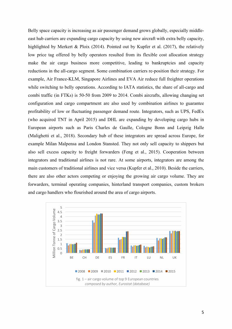
5

Belly space capacity is increasing as air passenger demand grows globally, especially middle-

east hub carriers are expanding cargo capacity by using new aircraft with extra belly capacity,

highlighted by Merkert & Ploix (2014). Pointed out by Kupfer et al. (2017), the relatively

low price tag offered by belly operators resulted from its flexible cost allocation strategy

make the air cargo business more competitive, leading to bankruptcies and capacity

reductions in the all-cargo segment. Some combination carriers re-position their strategy. For

example, Air France-KLM, Singapore Airlines and EVA Air reduce full freighter operations

while switching to belly operations. According to IATA statistics, the share of all-cargo and

combi traffic (in FTKs) is 50-50 from 2009 to 2014. Combi aircrafts, allowing changing set

configuration and cargo compartment are also used by combination airlines to guarantee

profitability of low or fluctuating passenger demand route. Integrators, such as UPS, FedEx

(who acquired TNT in April 2015) and DHL are expanding by developing cargo hubs in

European airports such as Paris Charles de Gaulle, Cologne Bonn and Leipzig Halle

(Malighetti et al., 2018). Secondary hub of these integrators are spread across Europe, for

example Milan Malpensa and London Stansted. They not only sell capacity to shippers but

also sell excess capacity to freight forwarders (Feng et al., 2015). Cooperation between

integrators and traditional airlines is not rare. At some airports, integrators are among the

main customers of traditional airlines and vice versa (Kupfer et al., 2010). Beside the carriers,

there are also other actors competing or enjoying the growing air cargo volume. They are

forwarders, terminal operating companies, hinterland transport companies, custom brokers

and cargo handlers who flourished around the area of cargo airports.

00.51

1.52

2.53

3.54

4.55

BE CH DE ES FR IT LU NL UKMillionTonn

eofCargoVolum

e

fig.1– aircargovolumeoftop9Europeancountries

composedbyauthor,Eurostat(database)

2008 2009 2010 2011 2012 2013 2014 2015

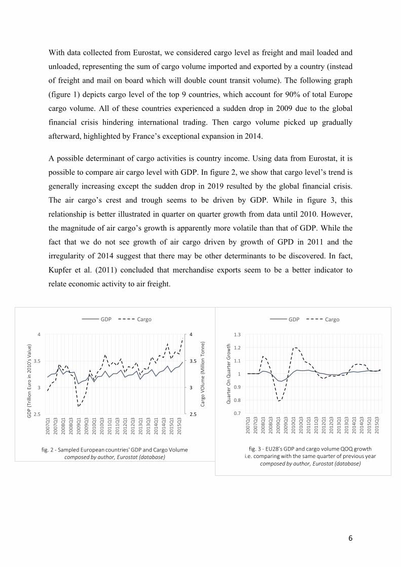
6

With data collected from Eurostat, we considered cargo level as freight and mail loaded and

unloaded, representing the sum of cargo volume imported and exported by a country (instead

of freight and mail on board which will double count transit volume). The following graph

(figure 1) depicts cargo level of the top 9 countries, which account for 90% of total Europe

cargo volume. All of these countries experienced a sudden drop in 2009 due to the global

financial crisis hindering international trading. Then cargo volume picked up gradually

afterward, highlighted by France’s exceptional expansion in 2014.

A possible determinant of cargo activities is country income. Using data from Eurostat, it is

possible to compare air cargo level with GDP. In figure 2, we show that cargo level’s trend is

generally increasing except the sudden drop in 2019 resulted by the global financial crisis.

The air cargo’s crest and trough seems to be driven by GDP. While in figure 3, this

relationship is better illustrated in quarter on quarter growth from data until 2010. However,

the magnitude of air cargo’s growth is apparently more volatile than that of GDP. While the

fact that we do not see growth of air cargo driven by growth of GPD in 2011 and the

irregularity of 2014 suggest that there may be other determinants to be discovered. In fact,

Kupfer et al. (2011) concluded that merchandise exports seem to be a better indicator to

relate economic activity to air freight.

2.5

3

3.5

4

2.5

3

3.5

4

2007

Q1

2007

Q3

2008

Q1

2008

Q3

2009

Q1

2009

Q3

2010

Q1

2010

Q3

2011

Q1

2011

Q3

2012

Q1

2012

Q3

2013

Q1

2013

Q3

2014

Q1

2014

Q3

2015

Q1

2015

Q3

CargoVOlume(MillionTonne)

GDP(TrillionEuroin2010'sValue)

fig.2- SampledEuropeancountries'GDPandCargoVolume


GDP Cargo

0.7

0.8

0.9

1

1.1

1.2

1.3

2007

Q1

2007

Q3

2008

Q1

2008

Q3

2009

Q1

2009

Q3

2010

Q1

2010

Q3

2011

Q1

2011

Q3

2012

Q1

2012

Q3

2013

Q1

2013

Q3

2014

Q1

2014

Q3

2015

Q1

2015

Q3

QuarterOnQuarterGrowth

fig.3- EU28’sGDPandcargovolumeQOQgrowth

i.e.comparingwiththesamequarterofpreviousyear


GDP Cargo

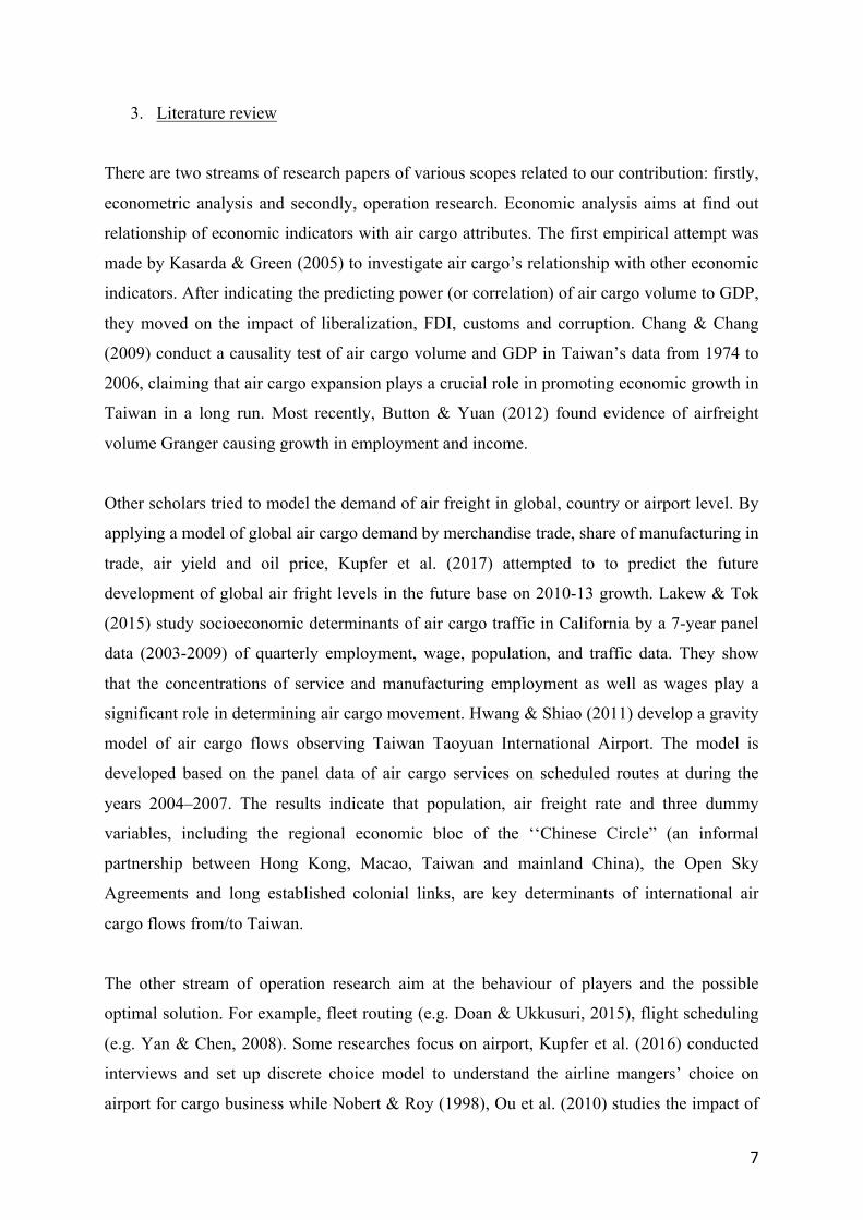
7


There are two streams of research papers of various scopes related to our contribution: firstly,

econometric analysis and secondly, operation research. Economic analysis aims at find out

relationship of economic indicators with air cargo attributes. The first empirical attempt was

made by Kasarda & Green (2005) to investigate air cargo’s relationship with other economic

indicators. After indicating the predicting power (or correlation) of air cargo volume to GDP,

they moved on the impact of liberalization, FDI, customs and corruption. Chang & Chang

(2009) conduct a causality test of air cargo volume and GDP in Taiwan’s data from 1974 to

2006, claiming that air cargo expansion plays a crucial role in promoting economic growth in

Taiwan in a long run. Most recently, Button & Yuan (2012) found evidence of airfreight

volume Granger causing growth in employment and income.

Other scholars tried to model the demand of air freight in global, country or airport level. By

applying a model of global air cargo demand by merchandise trade, share of manufacturing in

trade, air yield and oil price, Kupfer et al. (2017) attempted to to predict the future

development of global air fright levels in the future base on 2010-13 growth. Lakew & Tok

(2015) study socioeconomic determinants of air cargo traffic in California by a 7-year panel

data (2003-2009) of quarterly employment, wage, population, and traffic data. They show

that the concentrations of service and manufacturing employment as well as wages play a

significant role in determining air cargo movement. Hwang & Shiao (2011) develop a gravity

model of air cargo flows observing Taiwan Taoyuan International Airport. The model is

developed based on the panel data of air cargo services on scheduled routes at during the

years 2004–2007. The results indicate that population, air freight rate and three dummy

variables, including the regional economic bloc of the ‘‘Chinese Circle” (an informal

partnership between Hong Kong, Macao, Taiwan and mainland China), the Open Sky

Agreements and long established colonial links, are key determinants of international air

cargo flows from/to Taiwan.

The other stream of operation research aim at the behaviour of players and the possible

optimal solution. For example, fleet routing (e.g. Doan & Ukkusuri, 2015), flight scheduling

(e.g. Yan & Chen, 2008). Some researches focus on airport, Kupfer et al. (2016) conducted

interviews and set up discrete choice model to understand the airline mangers’ choice on

airport for cargo business while Nobert & Roy (1998), Ou et al. (2010) studies the impact of

8

manpower and truck scheduling in terminal operation, specifically Merkert & Ploix (2014)

investigated the importance of belly-hold freight. Boonekamp & Guillaume (2017) rank

airports by capturing all possible air freight connections by connectivity model base on

distance, time and frequency of operations while Mayer R. (2016) tried to categorize airports

by cluster analysis using the share of air cargo activity in different dimensions. There are also

literature investigating the revenue of carriers, for example Kasilingam (1997), Chao & Li

(2017), Lin et al. (2017). Additionally, Yuen et al. (2017) discussed about gateway and

hinterland airport. They suggest that there is potential competition and also cooperation

among airports considering the Pearl River Delta region in China.

Contributions in both research streams have not explored yet the possible effect of some

variables on cargo activity, such as the impact of e-commerce. Hence, our paper is a first

attempt trying to fill this gap.

4. Empirical Strategy

As mentioned in the introduction, this paper is aiming at finding out the determinants of air

cargo traffic at the country level, and aiming at drawing some policy implications. We define

research questions to achieve such goal. Firstly, we consider determinants that may reflect

consumption ability. Income level of a country may enhance the purchasing power and the

total demand. Higher income of a country, which favor the fast but costly shipment reflected

by air cargo level, may explain the relationship between white collar employment and

demand of air cargo services. Hence, the following is our first research hypothesis.

RH1: The income of a country may be a positive determinant of air cargo level

Secondly, a strong growing element of air cargo industry is the express parcel carried as a

result of booming e-commerce. Integrator will be more willing to invest in a country where

local consumers are adapting such consumption mode quicker. Such purchasing pattern can

be reflected by the percentage of population once purchased online in a country: for this

reason, we investigate the following research hypothesis.

RH2: Online purchase activity may be a positive determinant of air cargo level.

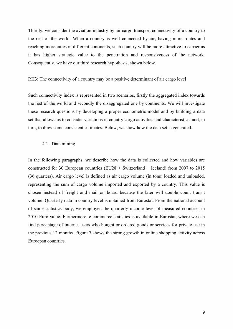
9

Thirdly, we consider the aviation industry by air cargo transport connectivity of a country to

the rest of the world. When a country is well connected by air, having more routes and

reaching more cities in different continents, such country will be more attractive to carrier as

it has higher strategic value to the penetration and responsiveness of the network.

Consequently, we have our third research hypothesis, shown below.

RH3: The connectivity of a country may be a positive determinant of air cargo level

Such connectivity index is represented in two scenarios, firstly the aggregated index towards

the rest of the world and secondly the disaggregated one by continents. We will investigate

these research questions by developing a proper econometric model and by building a data

set that allows us to consider variations in country cargo activities and characteristics, and, in

turn, to draw some consistent estimates. Below, we show how the data set is generated.

4.1 Data mining

In the following paragraphs, we describe how the data is collected and how variables are

constructed for 30 European countries (EU28 + Switzerland + Iceland) from 2007 to 2015

(36 quarters). Air cargo level is defined as air cargo volume (in tons) loaded and unloaded,

representing the sum of cargo volume imported and exported by a country. This value is

chosen instead of freight and mail on board because the later will double count transit

volume. Quarterly data in country level is obtained from Eurostat. From the national account

of same statistics body, we employed the quarterly income level of measured countries in

2010 Euro value. Furthermore, e-commerce statistics is available in Eurostat, where we can

find percentage of internet users who bought or ordered goods or services for private use in

the previous 12 months. Figure 7 shows the strong growth in online shopping activity across

Euroepan countries.

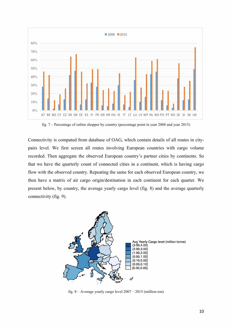
10

fig. 7 – Percentage of online shopper by country (percentage point in year 2008 and year 2015)

Connectivity is computed from database of OAG, which contain details of all routes in city-

pairs level. We first screen all routes involving European countries with cargo volume

recorded. Then aggregate the observed European country’s partner cities by continents. So

that we have the quarterly count of connected cities in a continent, which is having cargo

flow with the observed country. Repeating the same for each observed European country, we

then have a matrix of air cargo origin/destination in each continent for each quarter. We

present below, by country, the average yearly cargo level (fig. 8) and the average quarterly

connectivity (fig. 9).

fig. 8 – Average yearly cargo level 2007 – 2015 (million ton)

AT BE BG CY CZ DE DK EE ES FI FR GR HR HU IE IT LT LU LV MT NL NO PO PT RO SE SI SK UK0%

10%

20%

30%

40%

50%

60%

70%

80%

2008 2015

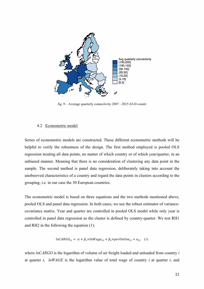
11

fig. 9 – Average quarterly connectivity 2007 - 2015 (O-D count)

4.2 Econometric model

Series of econometric models are constructed. These different econometric methods will be

helpful to verify the robustness of the design. The first method employed is pooled OLS

regression treating all data points, no matter of which country or of which year/quarter, in an

unbiased manner. Meaning that there is no consideration of clustering any data point in the

sample. The second method is panel data regression, deliberately taking into account the

unobserved characteristics of a country and regard the data points in clusters according to the

grouping, i.e. in our case the 30 European countries.

The econometric model is based on three equations and the two methods mentioned above,

pooled OLS and panel data regression. In both cases, we use the robust estimator of variance-

covariance matrix. Year and quarter are controlled in pooled OLS model while only year is

controlled in panel data regression as the cluster is defined by country-quarter. We test RH1

and RH2 in the following the equation (1):

!"#$%&'(,* = - + /0×!"2345(,* + /6×758'"!9"5(,* + :(,* (1)

where lnCARGO is the logarithm of volume of air freight loaded and unloaded from country i

at quarter t, lnWAGE is the logarithm value of total wage of country i at quarter t, and

12

perOnline is the percentage of individual of country i making online purchase in the last 12

months, yearly data is duplicated in the quarterly format.

Then there is a second set of equations to test RH1, RH2 and RH3. Moreover, there are two

specifications regarding connectivity. The first one includes a direct variable of general

connectivity, that becomes equation (2). CONN is the count of partner cities among all routes

of an observed country i in quarter t. Afterward, to further test the connectivity between

observed countries and cities in different continents, namely Africa (AF), Asia (AS), Latin

America (LA), Middle East (ME), North America (NA) and Europe (EU), we have the

following extended equation (3).

!"#$%&'(,* = - + /0×!"2345(,* + /6×758'"!9"5(,* + /;×#'<<(,* + :(,* (2)

!"#$%&'(,* = - + /0×!"2345(,* + /6×758'"!9"5(,* +=0×$>(,* + =6×$?(,* + =;×@$(,* + =A×BC(,* + =D×<$(,* + =D×CE(,* + :(,* (3)

For the second method of setting up a panel data, Hausman test confirms that fixed effect

model is appropriated by rejecting the unique errors (:(,*) are correlated with the regressors.

The additional equations with variable in fixed effect panel date, -( (n=1….30) the unknown

intercept for each country, are not reported for the reason of simplicity. For the same reason

the control variables of time are not shown in above equations.

Equations (1)-(3) present possible endogeneity problems, concentrated in the possible

inverted causal relation between wage (the proxy for income) and cargo activity. In order to

control for possible endogeneity we use a lagged variable for wage as instrument (presented

as equation 2bis in the section 6). In this way we can check whether the previous year wage

level in a specific country can determine the activity in air cargo in the current year. This

should be enough to eliminate possible distortions arising from endogeneity.

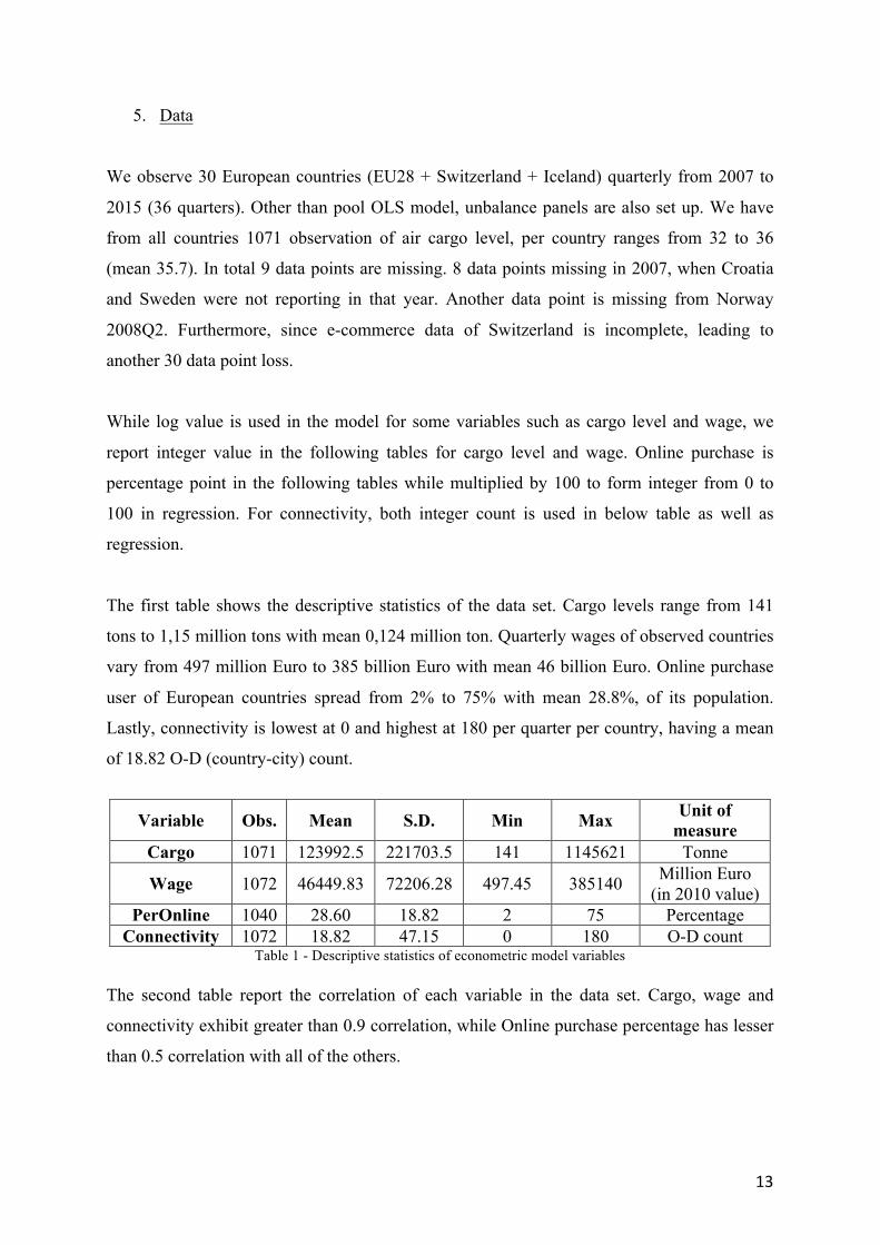
13

5. Data

We observe 30 European countries (EU28 + Switzerland + Iceland) quarterly from 2007 to

2015 (36 quarters). Other than pool OLS model, unbalance panels are also set up. We have

from all countries 1071 observation of air cargo level, per country ranges from 32 to 36

(mean 35.7). In total 9 data points are missing. 8 data points missing in 2007, when Croatia

and Sweden were not reporting in that year. Another data point is missing from Norway

2008Q2. Furthermore, since e-commerce data of Switzerland is incomplete, leading to

another 30 data point loss.

While log value is used in the model for some variables such as cargo level and wage, we

report integer value in the following tables for cargo level and wage. Online purchase is

percentage point in the following tables while multiplied by 100 to form integer from 0 to

100 in regression. For connectivity, both integer count is used in below table as well as

regression.

The first table shows the descriptive statistics of the data set. Cargo levels range from 141

tons to 1,15 million tons with mean 0,124 million ton. Quarterly wages of observed countries

vary from 497 million Euro to 385 billion Euro with mean 46 billion Euro. Online purchase

user of European countries spread from 2% to 75% with mean 28.8%, of its population.

Lastly, connectivity is lowest at 0 and highest at 180 per quarter per country, having a mean

of 18.82 O-D (country-city) count.

Variable Obs. Mean S.D. Min Max Unit of measure

Cargo 1071 123992.5 221703.5 141 1145621 Tonne

Wage 1072 46449.83 72206.28 497.45 385140 Million Euro (in 2010 value)

PerOnline 1040 28.60 18.82 2 75 Percentage Connectivity 1072 18.82 47.15 0 180 O-D count

Table 1 - Descriptive statistics of econometric model variables

The second table report the correlation of each variable in the data set. Cargo, wage and

connectivity exhibit greater than 0.9 correlation, while Online purchase percentage has lesser

than 0.5 correlation with all of the others.

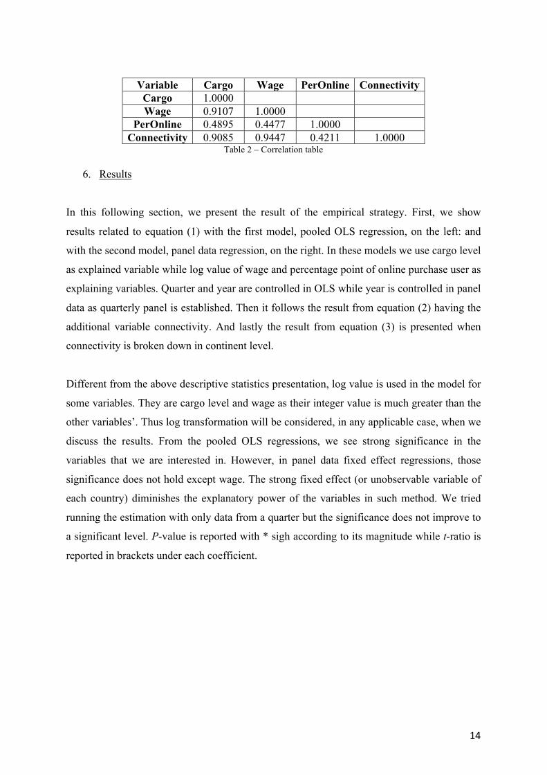
14

Variable Cargo Wage PerOnline Connectivity

Cargo 1.0000 Wage 0.9107 1.0000

PerOnline 0.4895 0.4477 1.0000 Connectivity 0.9085 0.9447 0.4211 1.0000

Table 2 – Correlation table

6. Results

In this following section, we present the result of the empirical strategy. First, we show

results related to equation (1) with the first model, pooled OLS regression, on the left: and

with the second model, panel data regression, on the right. In these models we use cargo level

as explained variable while log value of wage and percentage point of online purchase user as

explaining variables. Quarter and year are controlled in OLS while year is controlled in panel

data as quarterly panel is established. Then it follows the result from equation (2) having the

additional variable connectivity. And lastly the result from equation (3) is presented when

connectivity is broken down in continent level.

Different from the above descriptive statistics presentation, log value is used in the model for

some variables. They are cargo level and wage as their integer value is much greater than the

other variables’. Thus log transformation will be considered, in any applicable case, when we

discuss the results. From the pooled OLS regressions, we see strong significance in the

variables that we are interested in. However, in panel data fixed effect regressions, those

significance does not hold except wage. The strong fixed effect (or unobservable variable of

each country) diminishes the explanatory power of the variables in such method. We tried

running the estimation with only data from a quarter but the significance does not improve to

a significant level. P-value is reported with * sigh according to its magnitude while t-ratio is

reported in brackets under each coefficient.

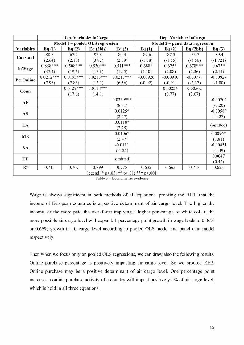
15

Dep. Variable: lnCargo Dep. Variable: lnCargo Model 1 – pooled OLS regression Model 2 – panel data regression

Variables Eq (1) Eq (2) Eq (2bis) Eq (3) Eq (1) Eq (2) Eq (2bis) Eq (3)

Constant 88.8 67.2 97.8 80.4 -89.6 -87.5 -63.7 -89.4 (2.64) (2.18) (3.82) (2.39) (-1.58) (-1.55) (-3.56) (-1.721)

lnWage 0.858*** 0.508*** 0.530*** 0.511*** 0.688* 0.675* 0.678*** 0.673* (37.4) (19.6) (17.6) (19.5) (2.10) (2.08) (7.36) (2.11)

PerOnline 0.0212*** 0.0193*** 0.0213*** 0.0217*** -0.00926 -0.00910 -0.00779 -0.00924 (7.96) (7.86) (12.1) (6.56) (-0.92) (-0.91) (-2.37) (-1.00)

Conn 0.0129*** 0.0118*** 0.00234 0.00562 (17.6) (14.1) (0.77) (3.07)

AF 0.0339*** -0.00202

(8.81) (-0.20)

AS 0.0125* -0.00589

(2.47) (-0.27)

LA 0.0118* (omitted) (2.25)

ME 0.0106* 0.00967

(2.47) (1.81)

NA -0.0111 -0.00451

(-1.25) (-0.49)

EU (omitted) 0.0047

(0.42) R2 0.715 0.767 0.799 0.775 0.632 0.663 0.718 0.623

legend: * p<.05; ** p<.01; *** p<.001 Table 3 – Econometric evidence

Wage is always significant in both methods of all equations, proofing the RH1, that the

income of European countries is a positive determinant of air cargo level. The higher the

income, or the more paid the workforce implying a higher percentage of white-collar, the

more possible air cargo level will expand. 1 percentage point growth in wage leads to 0.86%

or 0.69% growth in air cargo level according to pooled OLS model and panel data model

respectively.

Then when we focus only on pooled OLS regressions, we can draw also the following results.

Online purchase percentage is positively impacting air cargo level. So we proofed RH2,

Online purchase may be a positive determinant of air cargo level. One percentage point

increase in online purchase activity of a country will impact positively 2% of air cargo level,

which is hold in all three equations.

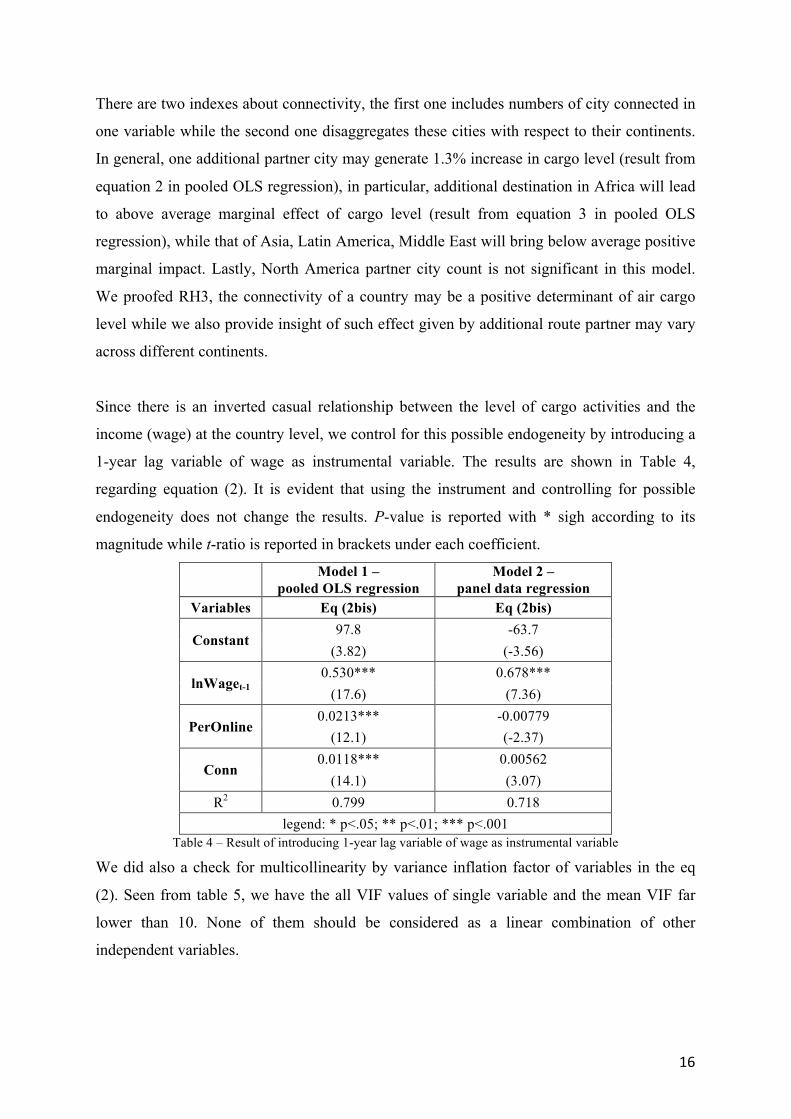
16

There are two indexes about connectivity, the first one includes numbers of city connected in

one variable while the second one disaggregates these cities with respect to their continents.

In general, one additional partner city may generate 1.3% increase in cargo level (result from

equation 2 in pooled OLS regression), in particular, additional destination in Africa will lead

to above average marginal effect of cargo level (result from equation 3 in pooled OLS

regression), while that of Asia, Latin America, Middle East will bring below average positive

marginal impact. Lastly, North America partner city count is not significant in this model.

We proofed RH3, the connectivity of a country may be a positive determinant of air cargo

level while we also provide insight of such effect given by additional route partner may vary

across different continents.

Since there is an inverted casual relationship between the level of cargo activities and the

income (wage) at the country level, we control for this possible endogeneity by introducing a

1-year lag variable of wage as instrumental variable. The results are shown in Table 4,

regarding equation (2). It is evident that using the instrument and controlling for possible

endogeneity does not change the results. P-value is reported with * sigh according to its

magnitude while t-ratio is reported in brackets under each coefficient.

Model 1 – pooled OLS regression

Model 2 – panel data regression

Variables Eq (2bis) Eq (2bis)

Constant 97.8 -63.7

(3.82) (-3.56)

lnWaget-1 0.530*** 0.678***

(17.6) (7.36)

PerOnline 0.0213*** -0.00779

(12.1) (-2.37)

Conn 0.0118*** 0.00562

(14.1) (3.07) R2 0.799 0.718

legend: * p<.05; ** p<.01; *** p<.001 Table 4 – Result of introducing 1-year lag variable of wage as instrumental variable

We did also a check for multicollinearity by variance inflation factor of variables in the eq

(2). Seen from table 5, we have the all VIF values of single variable and the mean VIF far

lower than 10. None of them should be considered as a linear combination of other

independent variables.

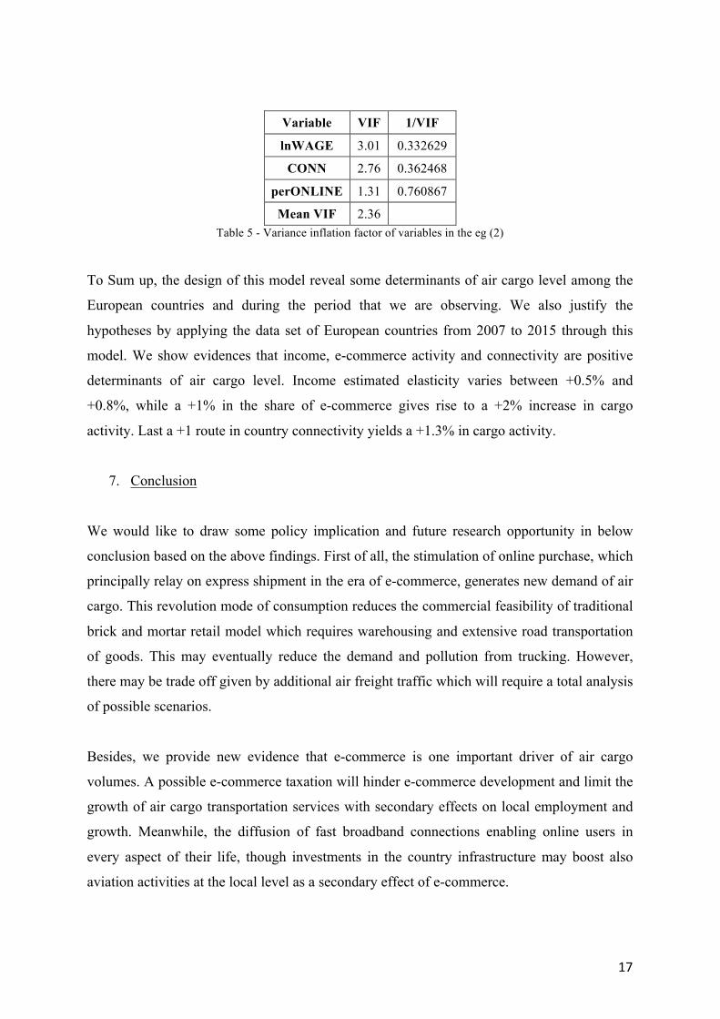
17

Variable VIF 1/VIF

lnWAGE 3.01 0.332629

CONN 2.76 0.362468

perONLINE 1.31 0.760867

Mean VIF 2.36 Table 5 - Variance inflation factor of variables in the eg (2)

To Sum up, the design of this model reveal some determinants of air cargo level among the

European countries and during the period that we are observing. We also justify the

hypotheses by applying the data set of European countries from 2007 to 2015 through this

model. We show evidences that income, e-commerce activity and connectivity are positive

determinants of air cargo level. Income estimated elasticity varies between +0.5% and

+0.8%, while a +1% in the share of e-commerce gives rise to a +2% increase in cargo

activity. Last a +1 route in country connectivity yields a +1.3% in cargo activity.

7. Conclusion

We would like to draw some policy implication and future research opportunity in below

conclusion based on the above findings. First of all, the stimulation of online purchase, which

principally relay on express shipment in the era of e-commerce, generates new demand of air

cargo. This revolution mode of consumption reduces the commercial feasibility of traditional

brick and mortar retail model which requires warehousing and extensive road transportation

of goods. This may eventually reduce the demand and pollution from trucking. However,

there may be trade off given by additional air freight traffic which will require a total analysis

of possible scenarios.

Besides, we provide new evidence that e-commerce is one important driver of air cargo

volumes. A possible e-commerce taxation will hinder e-commerce development and limit the

growth of air cargo transportation services with secondary effects on local employment and

growth. Meanwhile, the diffusion of fast broadband connections enabling online users in

every aspect of their life, though investments in the country infrastructure may boost also

aviation activities at the local level as a secondary effect of e-commerce.

18

Furthermore, liberalization in air transport enhance the flexibility of network, lowering the

barrier of carriers to reach out new destinations. The connectivity improvement will again

contribute to the supply of capacity and lowering the cost. Such relationship was seen in

passenger flow. In this research we highlight the importance of connectivity to air cargo level

while a deeper understand of such dynamic and a complete data base of more detailed O-D

information will better define also the relationship of air cargo volume and liberalization.

Moreover, the result of this study can be useful to governors who may want to compete air

cargo traffic share by facilitating e-commerce convenience and popularity, and to airline

managers who may want to spot new cargo hub regarding the country’s income level.

Concerning connectivity, we also hinted the different degree of impact given by additional

route partner city in different continents. It will be very interesting to investigate also the type

of good which is transported between these countries to better illustrate the dynamic of air

cargo transportation and the interdependence among economies. This may also eventually

guide airline managers to build up a long term strategy for the air cargo network.

Last but not least, we would like to highlight the limitation and potential improvements of

this paper. Income is the strongest indicator among the variables in the model while the rest

of them are less significant in panel data. We agreed that there could be correlation or

unobservable variable issues. A more elaborated data set may possible solve the issue when

data about manufacturing goods movement by air, e-commerce trading path, air cargo

movement by carrier category and route would be available. However, these are all privately

ran business, therefore publication of such data is not strictly required by governments. To

tackle unobserved variable in country level, future researches may move toward catchment

area of air cargo airports, manufacturing activity, integrator presence or

cooperation/competition with neighboring countries.

19

Reference ATAG (2018) Aviation Benefits Beyond Boarders Boonekamp T. & Burghouwt G., (2017) Measuring connectivity in the air freight industry, Journal of Air Transport Management 61, 81-94 Boeing’s World Air Cargo Forecast 2016-2017 Brugnoli A., Dal Bianco A., Martini G., Scotti D., (2018) The impact of air transportation on trade flows: A natural experiment on causality applied to Italy, Transportation Research Part A 112, 95-107 Button K. & Taylor S., (2000) International Air Transportation and Economic Development, Journal of Air Transport Management 6, 209-222 Button K. & Yuan J., (2012) Airfreight Transport and Economic Development: An Examination of Causality, Urban Studies 50, 329-340 Chang Y.H. & Chang Y.W., (2009) Air Cargo Expansion and Economic Growth: Finding the Empirical Link, Journal of Air Transport Management 15, 264-265 Chao C.C. & Li R.G., (2017) Effects of cargo types and load efficiency on airline cargo revenues, Journal of Air Transport Management 61, 26-33 Doan K. & Ukkusuri S.V., (2015) Dynamic system optimal model for multi-OD traffic networks with an advanced spatial queuing model, Transportation Research Part C 51, 41-65 Feng B., Li Y., Shen Z.M. (2015) Air cargo operations: Literature review and comparison with practices, Transportation Research Part C 56, 263–280 Hwang C.C. & Shiao G.C., (2011) Analyzing air cargo flows of international routes: an empirical study of Taiwan Taoyuan International Airport, Journal of Transport Geography 19 (2011) 738–744 Hummels D. (2008) Global Trends in Trade and Transportation, 17th Symposium – Benefiting from Globalisation, OECD Publishing Hummels D., Ishii J., Yi K.M., (1999) The Nature and Growth of Vertical Specialization in World Trade, Journal of International Economics 54, 75-96 IATA (2010-2015) World Air Transport Statistics (Various Editions). IATA (2017) Fact Sheet – Fuel ICAO (2015) Impact of Air Cargo Services on Economic Development Kasarda J.D. & Green J.D., (2005) Air Cargo as an Economic Development Engine: A Note on Opportunities and Constraints, Journal of Air Transport Management 11, 459-462

20

Kasilingam, R.G., (1997) An economic model for air cargo overbooking under stochastic capacity, Computers & Industrial Engineering 32, 221-226 Kupfer F., Meersman H., Onghena E., Van de Voorde E., (2010) World air cargo and merchandise trade, Critical Issues in Air Transport Economics and Business, Routledge, 98-111 Kupfer F., Meersman H., Onghena E., Van de Voorde E., (2011) Air freight and merchandise trade: towards a disaggregated analysis, Journal of Air Transport Studies 2, 28-48 Kupfer F., Kessels R., Goos P., Van de Voorde E., Verhetsel A., (2016) The origin–destination airport choice for all-cargo aircraft operations in Europe, Transportation Research Part E 87, 53-74 Kupfer F. Meersman H., Onghena E., Van de Voorde E., (2017) The underlying drivers and future development of air cargo, Journal of Air Transport Management 61, 6-14 Lakew P.A., Tok Y.C.A (2015) Determinants of air cargo traffic in California, Transportation Research Part A 80, 134–150 Li Z., Bookbinder J.H., Elhedhli S., (2012) Optimal shipment decisions for an airfreight forwarder: formulation and solution methods, Transportation Research Part C 21, 17–30 Lin D., Lee C.K.M., Yang J., (2017) Air cargo revenue management under buy-back policy , Journal of Air Transport Management 61, 53-63 Malighetti P., Martini G., Redondi R., Scotti D,. (2018) Integrators’ Air Transport Networks in Europe, Networks and Spatial Economics, 1-25 Mayer R. (2016) Airport classification based on cargo characteristics, Journal of Transport Geography 54 (2016) 53–65 Merkert R., Ploix B., (2014) The impact of terminal re-organisation on belly-hold freight operation chains at airports, Journal of Air Transport Management 36, 78-84 Nobert Y., Roy J., (1998) Freight handling personnel scheduling at air cargo terminals. Transportation Science 32 (3), 295–301 Ou J., Hsu V.N., Li C.L., (2010) Scheduling truck arrivals at an air cargo terminal, Production and Operations Manage 19, 83–97 Shepherd B., Shingal A., Raj A., (2016) Value of Air Cargo: Air Transport and Global Value Chains, IATA Sparks Bureau of Business and Economic Research, (2005) The Economic Impact of Memphis International Airport

21

Transportation Research Board (2009) Effective Practices for Preparing Airport Improvement Program Benefit-Cost Analysis Wisconsin DOT (2000) Benefit-Cost Analysis for the Rock County Airport (JVL) Runway Extension Yan S., Chen C.H., (2008) Optimal flight scheduling models for cargo airlines under alliances, Journal of Scheduling 11, 175–186. Yapar B.K., Bayrakdar S., Yapar M., (2015) The Role of Taxation Problems on the Development of E-Commerce, Procedia - Social and Behavioral Sciences 195, 642-648 Yuen A., Zhang A., Hui Y.V., Leung L.C., Fung M. (2017) Is developing air cargo airports in the hinterland the way of the future?, Journal of Air Transport Management 61,15-25