survey strategies for assessment of bering sea … strategies for assessment of bering sea forage...
TRANSCRIPT

NORTH PACIFIC RESEARCH BOARD PROJECT FINAL REPORT
Survey Strategies for Assessment of Bering Sea Forage Species
NPRB Project 401 Final Report
Michael F. Sigler1, Mark C. Benfield2, Evelyn D. Brown3, James H. Churnside4, Nicola Hillgruber5, John K. Horne6, Sandra Parker-Stetter6
1 National Oceanic & Atmospheric Administration, National Marine Fisheries Service, Alaska Fisheries Science Center, 11305 Glacier Highway, Juneau, AK 99801. (907) 789-6037, [email protected]. 2 Lousiana State University, Department of Oceanography and Coastal Sciences Coastal Fisheries Institute, 2179 Energy, Coast & Environment Bldg., Baton Rouge LA 70803, (225) 578-6372, [email protected] 3 University of Alaska, Fairbanks, School of Fisheries and Ocean Sciences Institute of Marine Science P.O. Box 757220, Fairbanks AK 99775-7220, (907) 590-2462, [email protected] 4 NOAA Environmental Technology Lab, 325 Broadway R/E/ET 1, Boulder CO 80303, (303) 497-6744, [email protected] School of Fisheries and Ocean Sciences, University of Alaska Fairbanks, 11120 Glacier Highway, Juneau, AK 99801, (907) 796-6288, [email protected] 6 University of Washington, School of Aquatic and Fishery Sciences, Box 355020, Seattle WA 98195, (206) 221-6890, [email protected] and [email protected]
July 2006

Abstract
Lack of information on forage species composition, distribution, and movements hinders
our understanding of their ecological role in the Bering Sea. Recognizing the need for
development of forage species survey strategies, this study characterized forage species in the
slope, shelf, and nearshore regions of the Bering Sea using direct (midwater trawl, MultiNet,
beach seine, jig, ROV) and indirect (acoustics, LIght Detection And Ranging (LIDAR))
sampling technologies. Forage species distribution and quantity differed between shelf (6-100 m)
and slope (6-100 m, 100-300 m, 300 m-bottom) regions. Acoustics suggest that shallow and deep
layers contained dispersed backscatter while the middle layer contained patchy schools. LIDAR
and visual measurements from aircraft documented a patchy distribution of surface plankton and
densely shoaling fish that exhibited a high degree of temporal and spatial variability within the
10 d study period. In the nearshore, Pacific sand lance dominated catches and other commonly
captured forage fish were YOY Pacific sandfish and gadids. Zooplankton density in the upper
100 m of the water column was significantly higher in nearshore waters. Though copepods were
the most abundant taxa, euphausiids, second most abundant, provided more energy to predators
due to their large size. We identified several potential candidate species/groups for assessment
with acoustics and direct sampling. Other potential, near-surface species/groups could be
surveyed with LIDAR and direct sampling. Our results suggest that shelf, slope, and nearshore
regions should be surveyed separately and that additional work, in the form of species-or group-
specific temporal studies, should be undertaken to refine survey designs.
Key Words
bathylagids, myctophids, Pacific sandfish, Pacific sand lance, squid, euphausiids, copepods,
acoustics, aerial remote sensing, LIDAR
Citation
Sigler, M. F., M. C. Benfield, E. D. Brown, J. H. Churnside, N. Hillgruber, J. K. Horne, S.
Parker-Stetter. 2006. Survey Strategies for Assessment of Bering Sea Forage Species. North
Pacific Research Board Final Report 401, 137 p.
2

Table of Contents
Study Chronology ....................................................................................................................................... 4 Introduction................................................................................................................................................. 4 Goal and Objectives .................................................................................................................................... 5
Chapter 1. Characterizing distribution and identity of nekton in shelf and slope habitats of the Bering
Sea............................................................................................................................................................. 6 Chapter 2. Forage fish in shallow nearshore habitats of the Bering Sea .................................................. 6 Chapter 3. Distribution, composition and energy density of zooplankton in the southeastern Bering Sea
.................................................................................................................................................................. 6 Chapter 4. Aerial remote sensing and ecological hot spots in the southeastern Bering Sea ................... 6 Chapter 5. Mesozooplankton distributions in the southeastern Bering Sea estimated using a Multinet
sampler and an evaluation of semi-automated processing with ZooImage software................................ 6 Conclusions .................................................................................................................................................. 6 Nekton in Shelf and Slope Habitats ............................................................................................................ 6
Shelf and Slope Habitats ........................................................................................................................... 7 Technology Comparisons ......................................................................................................................... 7 Biological Hotspots................................................................................................................................... 8 Zooplankton Composition and Energetics ................................................................................................ 8
Nearshore Habitat........................................................................................................................................ 9 Publications ................................................................................................................................................. 9 Outreach .................................................................................................................................................... 10 Acknowledgements ................................................................................................................................... 10 Literature Cited ........................................................................................................................................ 11
3
Study Chronology
This project began October 1, 2004 and ended April 30, 2006. The first study year was
devoted to study design and cruise preparation. Fieldwork occurred during June 2005. The
second study year was devoted to laboratory analysis, quantitative data analysis, and report
writing. Progress reports were submitted January 2005, July 2005, and January 2006.
Introduction
While the importance of forage species to a healthy ecosystem is widely accepted,
targeted and comprehensive studies in the Bering Sea and Gulf of Alaska are limited or lacking.
In 1999, amendments to Alaskan groundfish management plans created a forage fish category to
allow for specific management actions intended to conserve and manage forage species
resources. Without critical life history, distribution, and abundance information the effects of
management actions on these species cannot be understood and may not be detectable given the
assessment tools currently used. Forage species occupy all major habitats of the Bering Sea:
demersal, pelagic, meso- and epi-pelagic, and nearshore. The diverse life histories, distributions,
and population dynamics of these species likely will require a diverse array of survey designs
and assessment techniques to manage and protect forage species.
Mesopelagic species such as squids and myctophids are an important component of the
Bering Sea ecosystem (Sinclair and Stabeno, 2002). Most species are found in water deeper than
250 m during the day and vertically migrate towards the surface at night, often reaching the 100
m upper layer (Watanabe et al., 1999). Few assessment or ecological studies have targeted these
species, despite their importance in the diet of many predators including pinnipeds, cetaceans,
seabirds, and finfish (Kajimura and Loughlin, 1988; Hunt et al., 1996; Brodeur et al., 1999).
Standard research assessment surveys by the Alaska Fisheries Science Center (AFSC) usually
operate during daylight hours during the summer, using sampling techniques that do not
explicitly census mesopelagic species.
Information also is scarce on the use of nearshore habitats (e.g., eelgrass, kelp) by forage
species. The rugged Alaskan coastline combined with adverse weather makes extensive sampling
in nearshore habitats difficult. Of the few studies done within the Bering Sea, key forage species
captured include capelin (Mallotus villosus), Pacific cod (Gadus macrocephalus), Pacific herring
(Clupea pallasi), Pacific sand lance (Ammodytes hexapterus), surf smelt (Hypomesus pretiosus),
4

and walleye pollock (Theragra chalcogramma) (Isakson et al., 1971; Hancock, 1975;
Naumenko, 1996; Robards, 1999; Robards and Schroeder, 2000). It is known that various smelt
species migrate to nearshore areas to spawn. In the southeastern Bering Sea, capelin spawning
has been reported in Port Moller (Warner and Shafford, 1978), and the Togiak area, beginning in
mid-May and lasting until late June (Pahlke, 1985). In Prince William Sound, age-0 and age-1
capelin are found in nearshore nursery areas (Brown, 2002). In addition to providing habitat for
spawning adults of some species, nearshore areas also function as migratory pathways and
nursery environments for larval and juvenile forage fish, particularly those areas that offer
structured habitat (e.g., eelgrass beds).
Assessing distributions and abundances of forage species requires the use of single or
multiple sampling technologies depending on the species and/or habitat of interest. Catches of
forage species have occurred during annual bottom trawl surveys (Livingston, 2002), acoustic-
trawl surveys (Honkalehto et al., 2002), and surface trawl surveys (Farley et al., 2000).
Dedicated survey efforts have not been directed towards forage species. In this pilot study, we
applied, compared, and potentially integrated a suite of survey techniques over a continuum of
forage species habitats. These technologies consisted of high-frequency acoustics (38 and 120
kHz), mid-water trawling, seining, MultiNet zooplankton sampling1, in-situ imaging, and aerial
remote sensing including airborne LIDAR.
Goal and Objectives
The goal of this project was to assess the distribution, species composition, and
ecological role of forage species within nearshore, continental shelf, and continental slope
habitats, and the technologies and techniques used to collect the data. Specific objectives
included:
1) Apply a suite of survey techniques to assess the distribution, species composition, and diet of
forage species from nearshore to continental slope habitats.
2) Identify strengths and constraints of integrating survey techniques to optimize habitat-specific
survey effort.
1 Unfortunately, components of our in-situ imaging system (ZOOVIS-SC) were damaged during shipping and the system was not operational during our research cruise.
5
Manuscripts
Chapter 1. Characterizing distribution and identity of nekton in shelf and slope habitats of the
Bering Sea
Chapter 2. Forage fish in shallow nearshore habitats of the Bering Sea
Chapter 3. Distribution, composition and energy density of zooplankton in the southeastern
Bering Sea
Chapter 4. Aerial remote sensing and ecological hot spots in the southeastern Bering Sea
Chapter 5. Mesozooplankton distributions in the southeastern Bering Sea estimated using a
Multinet sampler and an evaluation of semi-automated processing with ZooImage software
Conclusions
Assessing forage species in the slope, shelf and nearshore regions of the Bering Sea is
essential for both ecological understanding and effective resource management. Our study
results suggest that these regions differ in their species composition and distribution over time
and space. We identified several potential candidate species/groups for population abundance
estimates with acoustics and direct sampling. Other potential, near-surface species/groups could
be surveyed with LIDAR and direct sampling. Based on our results, in general we recommend
that shelf, slope and nearshore regions should be surveyed separately and that additional work, in
the form of species-specific temporal studies should be undertaken to refine survey designs.
Specific recommendations by habitat follow.
Nekton in Shelf and Slope Habitats
Population abundance assessment of mesopelagic species in the Bering Sea is important
from an ecosystem and resource management perspective. Previous studies, such as Sinclair and
Stabeno (2002), provide a limited picture of nekton distribution due to the use of single trawl
hauls. By combining acoustics, LIDAR, and direct sampling, our June 2005 survey highlights
6

aspects of nekton distribution that will assist in the development of assessment strategies and
quantitative abundance estimates for Bering Sea mesopelagic nekton species.
Shelf and Slope Habitats
1. Shelf and slope regions should be surveyed separately. Nekton horizontal and vertical
distribution differed between the two regions, making it necessary to design region-
specific surveys.
Technology Comparisons
2. In this study, backscatter measurements from acoustics and LIDAR did not match and
could not be combined to provide a full water column numeric/biomass estimate.
Additional LIDAR calibration and experimental measurements are needed to facilitate
direct comparison between acoustic and optic backscatter data.
3. Acoustics samples backscatter from transducer face through the entire water column.
Time needed to sample any area is restricted by platform speed.
4. LIDAR should be restricted to assessment of near-surface (<30 m) forage species or
species that vertically migrate into surface waters at night. Aircraft-mounted LIDAR can
synoptically sample large areas.
5. Surveys of Bering Sea mesopelagic species must include direct sampling for target
identification and specimen collection.
6. Several potential candidate species/groups for population abundance estimates were
identified: deepwater myctophids and bathylagids, shelf break squid and Pacific ocean
perch (Sebastes alutus), shelf herring, walleye pollock, and slope pelagic walleye
pollock.
7. Dedicated species- or group-specific pilot surveys are necessary to obtain accurate target
strength estimates for separating: myctophids versus bathylagids, herring or capelin
versus walleye pollock, and squid versus Pacific ocean perch.
8. Target species or groups should be observed at different times -daylight, crepuscular, and
dark - as the effect of vertical or horizontal migration on assessment results cannot be
determined at this time. Predictable diel movements could also provide additional ways
to characterize the mesopelagic community composition.
7

9. Appropriate transect spacing must be determined for target species or groups. Ranges
observed during our spatiotemporal analyses (2.4 – 5.6 km) suggest that 1 nmi transect
spacing was too large to capture backscatter spatial structure in some depth layers.
10. Specific surveys should be undertaken to evaluate the contribution of jellyfish to the
mesopelagic community. Midwater trawl catches frequently included jellyfish, but our
gear did not effectively sample these organisms
Biological Hotspots
11. Airborne estimates of birds and mammals were obtained and high concentrations of these
predators were associated with the moving masses of fish (presumably capelin) and large
aggregations of swarming euphausiids (e.g., hot spots). Hot spots were approximately 5
nmi in diameter and were concentrated on the shelf near the shelf break. Several formed
and disappeared within our relatively short survey period. Assessments of horizontally
migrating concentrations should not be done within pre-determined, fixed regions, but
rather within adaptively moving grids that can track the biomass.
12. Moving masses of fish schools resembling capelin and Atka mackerel (Pleurogrammus
monopterygius) (identified by local fishing vessels) were observed from the aircraft but
were not directly sampled. Most of these schools were outside the region sampled by the
ship.
Zooplankton Composition and Energetics
13. Zooplankton and micronekton in the southeastern Bering Sea was dominated by
copepods, followed by euphausiids, pteropods, and larvaceans, all of which represent
important prey items of forage taxa diet.
14. Since estimates of species abundance and composition varied substantially between shelf
and slope stations, assessment of forage taxa prey field needs to be stratified by sampling
area.
15. Since many prey taxa migrate vertically on a diurnal basis, it is essential to survey them
at different times of the day in order to accurately assess abundance and availability of
prey to forage species.
16. The predominance of juvenile stages of euphausiids in the samples might be an artifact of
increased net avoidance behavior with ontogeny, making it necessary to employ nets with
a larger opening to accurately assess euphausiids abundance.
8

17. When assessing the zooplankton standing stock as a food resource for forage fish, the
inclusion of energy content is important because variation amongst species in energy
density (kJ g-1) and size result in a different relative importance of taxa than estimated
from abundance measures alone.
18. Species-specific measures of energy content are better than grouping taxa, given that the
two pteropod species we analyzed had the most disparate energy density amongst all
species examined.
Nearshore Habitat
Our study showed that shallow nearshore fish assemblages on Akutan, Akun, and
Unalaska Islands in June were dominated by forage fish, particularly Pacific sand lance. Most
sand lance we captured were juveniles and were from sand habitat, whereas all Pacific sandfish
and gadids were young-of-the-year and most were from cobble habitat. The fewest number of
fish were captured in bedrock habitat.
The survey approach and sampling techniques we applied were successful at sampling
nearshore habitats. We recommend that this approach be continued in studies of nearshore
habitats of Bering Sea forage species. One unsurprising result was that some potential nearshore
species such as capelin were not found. This lack likely is due to timing of the survey as some
nearshore species occupy nearshore habitats only seasonally and only one time period was
sampled in this pilot study. Our second recommendation is to expand sampling to multiple time
periods in future nearshore sampling. Seasonal studies would help define temporal use of
shallow nearshore habitats in the Bering Sea by forage fish species and is a common approach
for nearshore habitat sampling (Johnson et al., 2005).
Publications
The five chapters are intended for publication in peer-reviewed journals.
9
Outreach
Benfield, M.C. N. Hillgruber, P. Grosjean, M. Alford, S. Arndt, J. Bacon, and S.F. Keenan.
2006. Semi-automated processing of Bering Sea zooplankton samples using ZooImage
software. Poster presented at the 2006 Alaska Marine Science Symposium, 22-25 Jan 2006,
Anchorage, AK.
Parker-Stetter, S. 2006. Forage species in the Bering Sea. Webpage
http://www.acoustics.washington.edu/current_research.php#Stetter
Parker-Stetter, S., M. Benfield, E. Brown, J. Churnside, N. Hillgruber, J. Horne, S. Johnson, C.
Kenaley, M. Sigler, J. Thedinga, J. Vollenweider. 2006. Survey strategies for Bering Sea
forage species. Poster presented at the 2006 Alaska Marine Science Symposium, 22-25 Jan
2006, Anchorage, AK. http://www.acoustics.washington.edu/images/ParkerStetter_poster.pdf
Parker-Stetter, S., J. Horne, and J. Churnside. 2006. Acoustic and optic characterization of forage
fish distribution in the Bering Sea. Abstract submitted to Acoustical Society of America.
Thedinga, J. F., S.W. Johnson, M.R. Lindeberg, and A.D. Neff. 2006. Bering Sea forage fish: Do
they use the shallow nearshore?. Poster presented at the 2006 Alaska Marine Science
Symposium, 22-25 Jan 2006, Anchorage, AK.
Acknowledgements
We would like to thank the captains and crews of the F/V “Great Pacific” and the F/V “Kema
Sue” for their invaluable support at sea. Funding for this research was supported with a grant
from the North Pacific Research Board, project # F0401.
10

Literature Cited
Brodeur, R.D., Wilson, M.T., Walters, G.E., and Melnikov, I.V. 1999. Forage fishes in the
Bering Sea: distribution, species associations, and biomass trends. In: Loughlin, T.R. and
Ohtani, K. (Eds.). Dynamics of the Bering Sea. University of Alaska Sea Grant, Fairbanks,
pp. 509-536.
Brown, E. D. 2002. Life history, distribution, and size structure of Pacific capelin in Prince
William Sound and the northern Gulf of Alaska. ICES J. Mar. Sci. 59: 983-996.
Farley, E.V., Jr., Haight, R.E., Guthrie, C.M., and Pohl, J.E. 2000. Eastern Bering Sea (Bristol
Bay) coastal research on juvenile salmon, August 2000. (NPAFC Doc. 499).
Hancock, M. J. 1975. A survey of the fish fauna in the shallow marine waters of Clam Lagoon,
Adak, Alaska. M.S. Thesis, Florida Atlantic University, Boca Raton, FL.
Honkalehto, T., N. Williamson, D. McKelvey, and S. Stienessen. 2002. Results of the echo
integration-trawl survey for walleye pollock (Theragra chalcogramma) on the Bering Sea
shelf and slope in June and July 2002. NOAA/AFSC Processed Rep. 2002-04.
Hunt Jr., G. L., Decker, M.B., and Kitaysky, A.S. 1996. Fluctuations in the Bering Sea
ecosystem as reflected in the reproductive ecology and diets of kittiwakes on the Pribilof
Islands, 1975 to 1990. In: Greenstreets, S., and Tasker, M. (Eds.), Aquatic predators and their
prey. Blackwell, London, pp. 142-153.
Isakson, J.S., Simenstad, C.A., and Burgner, R.L. 1971. Fish communities and food chains in the
Amchitka area. Bio. Sci. 21: 666-670.
Johnson, S.W., A.D. Neff, and J.F. Thedinga. 2005. An atlas on the distribution and habitat of
common fishes in shallow nearshore waters of southeastern Alaska. U.S. Dep. Commer.,
NOAA Tech. Memo. NMFS-AFSC-139, 89 p.
11

Kajimura, H., and Loughlin, T.R. 1988. Marine mammals in the oceanic food web of the eastern
subarctic Pacific. In Nemoto, T., Pearcy, W.G. (Eds), The biology of the subarctic Pacific.
Bulletin of the Ocean Research Institute, University of Tokyo, 26 (II): 87-223.
Livingston, P. (ed.) 2002. Ecosystem considerations for 2003. Available
http://www.fakr.noaa.gov/npfmc/safes/safe.htm.
Naumenko, E. A. 1996. Distribution, biological condition and abundance of capelin (Mallotus
villosus) in the Bering Sea. In: Ecology of the Bering Sea: A review of Russian Literature, p.
237-256. Ed. O. A. Mathisen and K. O. Coyle. UA Sea Grant Program.
Pahlke, K. A. 1985. Preliminary study of capelin (Mallotus villosus) in Alaskan waters. ADFG
Info. Lflt. 250. 64 p.
Robards, M. 1999. Assessment of nearshore fish around Unalaska using beach seines during July
1999. USGS Biological Resources Division, Alaska.
Robards, M. and Schroeder, M. 2000. Assessment of nearshore fish around Akutan Harbor using
beach seines during March and July 2000. USGS Biological Resources Division, Alaska.
Sinclair, E.H. and Stabeno, P.J. 2002. Mesopelagic nekton and associated physics in the
southeastern Bering Sea. Deep-Sea Res. II 49: 6127-6146.
Warner, I. M. and Shafford P. 1978. Forage fish spawning surveys – southern Bering Sea.
Alaska marine environmental assessment project. Project completion report. ADFG Kodiak.
Watanabe, H., Masatoshi, M., Kawaguchi, K., Ishimaru, K., and Ohno, A. 1999. Diel vertical
migration of myctophid fishes (Family Myctophidae) in the transitional waters of the western
North Pacific. Fish. Oceanogr. 8(2): 115-127.
12

Chapter 1. Unpublished report: Do not cite without permission of authors.
Characterizing distribution and identity of nekton in shelf and slope regions of the Bering Sea
Sandra Parker Stetter1, John Horne1, James Churnside2, Nicola Hillgruber3, Michael Sigler4
1School of Aquatic and Fisheries Sciences, University of Washington, Seattle, WA 98195 2NOAA, Environmental Technology Laboratory, Boulder, CO 80303
3School of Fisheries and Ocean Sciences, University of Alaska Fairbanks, Juneau, AK 99801 4NOAA, Auke Bay Laboratory, Juneau, AK 99801
Abstract
Mesopelagic forage fish species are important components of the Bering Sea ecosystem,
but information on species distribution and identity is limited. Recognizing the need for
development of forage species survey strategies, we undertook this study to characterize nekton
in the slope and shelf regions of the Bering Sea using direct (midwater trawl, MultiNet) and
indirect (acoustics, LIght Detection And Ranging (LIDAR)) sampling technologies. Forage
species distribution and quantity differed between shelf (6-100 m) and slope (6-100 m, 100-300
m, 300 m-bottom) regions. Acoustic results suggest that shallow and deep depth zones contained
dispersed backscatter while the middle slope layer contained patchy schools associated with the
shelf break. Variogram results for repeated LIDAR surveys of the shelf and slope regions
indicate that backscatter distribution between 6-30 m was dynamic at the scale of days. This
result was expected given the strong frontal nature of the area. When LIDAR results were
compared with coincident acoustic transects on the shelf and slope, differences were found in
gear detection of backscatter. Acoustic results suggest that 25-63% of forage fish in the shelf
and slope regions were deeper than the LIDAR detection range. Although both LIDAR and
acoustics are constrained to portions of the water column, the utility of remote sampling
technologies is dependent on survey objectives. We identified several potential candidate
species/groups for population abundance estimates with acoustics and direct sampling. Other
potential, near-surface species/groups could be surveyed with LIDAR and direct sampling. Our
1

Chapter 1. Unpublished report: Do not cite without permission of authors.
results suggest that shelf and slope regions should be surveyed separately and that additional
work, in the form of species-or group-specific temporal studies, should be undertaken to refine
survey designs.
Introduction
Mesopelagic forage species such as myctophids, bathylagids, herring, and squid are
important components of the Bering Sea ecosystem (Sinclair and Stabeno 2002). Important in
the diets of many predators including pinnipeds, cetaceans, seabirds, skates, and finfish (e.g.,
Sinclair and et al. 1993, Hunt et al. 1996, Orlov 1998, Ohizumi et al. 2003), mesopelagic species
may influence predator foraging behavior with their dynamic diel movement patterns (e.g.,
Ohizumi et al. 2003, Sterling and Ream 2004).
While some work has addressed mesopelagic forage species in the Bering Sea (e.g.,
Balanov and Il’inskii 1992, Nagasawa et al. 1997, Watanabe et al. 1999, Sinclair and Stabeno
2002), comprehensive studies on forage species are limited. Existing information, based on
trawling, provides species composition (Sinclair and Stabeno 2002) and spatially discrete
biomass estimates of biomass (Nagasawa et al. 1997, Watanabe et al. 1999), but provides an
incomplete characterization of mesopelagic species. As a result, few large-scale estimates of
mesopelagic biomass exist (Balanov and Il’inskii 1992). This data gap limits Bering Sea
ecosystem models (Cianelli et al. 2004) and provides no context for estimates of marine mammal
consumption (e.g., Ohizumi et al. 2003).
In 1999, amendments to the National Marine Fisheries Service (NMFS) Alaskan
groundfish management plans created a specific category to conserve and manage forage species
resources. This forage fish category includes 59 fish species belonging to 8 families.
2

Chapter 1. Unpublished report: Do not cite without permission of authors.
Ecosystem-based management approaches require information on species distribution,
abundance, and life history attributes.
Single gear types (e.g., pelagic trawl, bottom trawl, gill nets, seines) have traditionally
been used to collect data for population estimates of single species. In this context, NMFS
research assessment surveys usually operate during daylight hours in the summer, using
sampling techniques that do not explicitly census mesopelagic species. As forage species occupy
all major habitats (bathy-, meso-, and epi-pelagic), the development of new, or modification of
existing, techniques is needed to directly assess the contribution of forage species to the Bering
Sea.
Methods
Study site
Systematic surveys of nekton were conducted at locations in continental shelf (<100 m)
and slope (100-1200 m) regions of the Bering Sea near Unalaska and Akutan Islands (Figure 1).
The slope region was surveyed 10-13 June 2005 and shelf region during 14-19 June 2005. Shelf
transects were spaced 0.5 nmi apart and slope transects were spaced 1.0 nmi apart (Figure 1). To
increase sampling intensity, higher resolution, adaptive surveys were intermittently conducted at
locations with high acoustic backscatter. Adaptive transect spacing varied with the target
assemblage. All data were collected aboard the F/V Great Pacific, a 38-m stern trawler with a
main engine of 1450 horsepower and a cruising speed of 10 kts.
3

Chapter 1. Unpublished report: Do not cite without permission of authors.
Acoustic data collection and processing
Acoustic data collection
Acoustic data were collected using a 38 kHz splitbeam echosounder (Simrad 38-12, input
power 2000 W, pulse length 1.024 ms, ping rate 1 sec-1), from 10-19 June 2005. We installed
the transducer on an YSI towed body suspended 2.5 m below the water surface and towed it at
approximately 6.0 kt. The echosounder was calibrated before our survey with a standard
tungsten carbide sphere using procedures outlined in Foote et al. (1987). Interference from
hydraulic winches and other machinery prevented acoustic data collection during deployment of
towed gear (midwater trawl, MultiNet).
Acoustic data processing
Echoview (v 3.30, SonarData 2005) was used to analyze all acoustic data. Transect files
were inspected for bottom delineation, vessel noise spikes, and electrical interference prior to
processing. CTD cast data were used to estimate absorption coefficients (Francois and Garrison
1982) and sound speed (Chen and Millero 1977).
EDSU selection and geostatistical approaches
We used a horizontal elemental distance sampling unit (EDSU) of 250 m for all analyses.
To determine this value, we initially exported slope-water-column and shelf Sv_mean for 10 m
horizontal cells. We assumed that spatial correlation in our data would not be at scales <10 m.
Preliminary variograms were inspected for nonstationarity and data sets were examined for
trends with direction (Northing, Easting, Northing•Easting) using forward stepping linear
regression. Final trend models were significant at R2 ≥ 0.05 and each parameter was significant
at P < 0.05. Trend effects were removed using a generalized linear model (GLM) with a
Gaussian error structure. Residuals were used to model the empirical spatial relationship among
4

Chapter 1. Unpublished report: Do not cite without permission of authors.
data points with classical or robust variogram procedures (Matheron 1963, Cressie and Hawkins
1980). Each variogram was fit, using a weighed least squares procedure (Cressie 1993), with
both exponential and spherical models. The best theoretical model was selected visually and the
fit of parameters was examined. The range of a spherical model and the effective range of an
exponential model indicate the distance (m) at which data are no longer spatially correlated. Our
EDSU data had ranges of 3.8 km in the slope region and 3.4 km in the shelf region. Horizontal
EDSU’s should not exceed one-half the range of the data (Rivoirard et al. 2000). A single
horizontal bin size of 250 m was chosen as the EDSU for both shelf and slope regions.
Nekton distribution
Acoustic data processing
Vertical depth strata, corresponding to shelf/shallow, shelf break, and deep-water regions,
were used in our analyses. We refer to these strata as shelf (6 m-bottom, where bottom ≤ 100),
slope-shallow (6-100 m), slope-middle (100-300 m), and slope-deep (300 m-bottom). For
comparison, we also included a slope-water-column stratum (6 m-bottom).
Two steps were taken to remove noise and restrict data to large nekton (i.e., fish and
squid). First, vessel noise was modeled through the water column with a 20•log(Range) time-
varied-threshold (TVT) using Sv @ 1m. Second, to restrict our analyses to large nekton (e.g.,
fish, squid), we applied a Sv minimum threshold to each depth strata. To do this, we calculated
the expected amount of volume backscatter (Sv) from an individual myctophid (the smallest fish
captured in trawl samples) in a single vertical sample (0.2 m). A target strength (TS, in dB) of -
52.5 dB (McClatchie and Dunford 2003) was selected based on similar sized myctophids to our
study. Expected Sv was calculated for each 1 m vertical bin within our 3 depth strata,
compensating for beam spreading and volume insonified. The median Sv value in each depth
5

Chapter 1. Unpublished report: Do not cite without permission of authors.
stratum was used as our minimum threshold: -66 dB (6-100 m), -77 dB (100-300 m), and -87 dB
(300 m-bottom). Samples with Sv less than either our vessel noise TVT or our Sv minimum
threshold were considered to have no detectable backscatter and were assigned -999 dB
(equivalent to 0 backscatter in linear domain, SonarData 2005).
Acoustic analysis of nekton distribution
We used daytime systematic transects in this analysis. Each depth stratum was treated
separately and data were exported by depth stratum in 250 m horizontal bins. Output values
included Sv_mean, Nautical Area Scattering Coefficient (NASC≡sA), and Area Backscattering
Coefficient (ABC≡sa). In the slope region, where data were exported in three depth strata, a
water column Sv_mean was calculated in each horizontal segment weighted by the proportion of
the water column occupied by each depth stratum.
We were interested in determining how large nekton, measured using Sv_mean, were
distributed in our survey area. We removed trends with direction (Northing, Easting, and/or
Northing•Easting), used the residuals to generate empirical variograms, and fit the empirical
variogram with theoretical models as outlined under EDSU selection and geostatistical
approaches.
Using trend (from GLM results) and spatial structure (from variogram models), we
predicted Sv_mean throughout our study area. Slope and shelf transects were surrounded with a
1-2 km box from the outer edges of the transects. A smaller box was created for the slope-deep
region. Bounding boxes were selected to provided outside distances of ~½ the transect spacing.
We then divided boxes into 250 m x 250 m grid cells. Using trend and variogram parameters
(sill, range, nugget), we predicted Sv_mean in boxes with universal kriging (Cressie 1993). All
geostatistical analyses were conducted using S-Plus 6.1 (Insightful Corporation 2002).
6

Chapter 1. Unpublished report: Do not cite without permission of authors.
Acoustic and optic spatiotemporal characterization of backscatter
Acoustics provided a detailed profile of the water column in slope and shelf regions over
several days. LIDAR offered a repeated, synoptic look at the same areas. We used the two data
sets to examine nekton distribution patterns among days or within depth layers. We were also
interested in comparing results and applications of the two techniques. Due to LIDAR depth
penetration, our comparative analyses were limited to the top 30 m of the water column.
Acoustic data processing
We used the same horizontal EDSU of 250 m determined for previous analyses. Five
vertical bins were used in all acoustic analyses: 6-12 m, 12-18 m, 18-24 m, 24-30 m, and 30 m-
bottom. For acoustics, the backscatter value exported was ABC. Data were transformed to loge
(≡lnABC) as ABC values span several orders of magnitude within each analysis.
For this analysis, we removed vessel noise and then exported data both with and without
an Sv minimum threshold. Vessel noise (Sv @ 1m) was modeled through the water column with
a 20•log(R) TVT and samples below this threshold were identified. Our first data set had no Sv
minimum thresholds to make it comparable to the LIDAR data. The second data set used
median Sv minimum thresholds for large nekton (-52.5 dB fish, based on McClatchie and
Dunford 2003), calculated at a 1 m vertical resolution within the 6-30 m depth range: -50 dB (6-
12 m), -54 dB (12-18 m), -57 dB (18-24 m), -60 dB (24-30 m), -66 dB (30-100 m), -77 dB (100-
300 m), and -87 dB (300 m-bottom). Samples with Sv less than our vessel noise TVT or our
nekton Sv minimum threshold were considered to have no detectable backscatter and were
assigned -999 dB (equivalent to 0 backscatter in linear domain, SonarData 2005).
7

Chapter 1. Unpublished report: Do not cite without permission of authors.
LIDAR data collection Aerial surveys of the slope/break systematic transects were performed 8, 9, 11, and 14
June during the day. A nighttime survey of the same region was performed in the early morning
of 13 June. Shelf systematic transects were surveyed during the day on 13, 17, 18, and 19 June
and at night on 17 June. A total of 12 flights were made between 8 and 19 June, with much of
the flight time devoted to covering a larger area of the shelf and slope. In total, almost 7900 km
were surveyed, with about 11% in the slope/break region and 16% in the shelf region as defined
in Fig. 1.
The LIDAR was the NOAA Fish LIDAR that has been described in detail elsewhere
(Churnside, et al, 2001; 2003; Churnside and Thorne, 2005). The system transmits a 12-nsec
pulse of linearly-polarized green (532 nm) light into the water. The return is detected in the
orthogonal linear polarization, and the temporal shape of the return is used to infer a depth
profile of scattering. The sampling swath is 5 m in diameter, which spreads out the energy so
that it is safe for marine mammals (Zorn, et al, 2000).
LIDAR data processing
Attenuation was inferred from the average slope of the logarithm of the signal
decay over a depth range chosen to minimize the effects of surface returns and noise. The
magnitude of the return from any depth was corrected for attenuation using this value. We then
processed the data to obtain the total backscatter level. Total return includes layers of
zooplankton or phytoplankton, diffuse aggregations of fish, and fish schools. The results within
the boundaries of the two acoustic-survey regions were selected. All data were exported with an
8

Chapter 1. Unpublished report: Do not cite without permission of authors.
ESDU of 250 m, and separated the data into 5 vertical bins: 2-6 m, 6-12 m, 12-18 m, 18-24 m,
and 24-30 m.
Spatiotemporal nekton distribution - 6 to 30 m
We compared backscatter distribution in acoustic and LIDAR data using trend and
geostatistical parameters. Analyses were restricted to depths (6-30 m) common to acoustics and
LIDAR and to the surface layer (2-6 m) from LIDAR analyses. Each depth layer was treated
separately in analyses. We removed trends with direction (Northing, Easting, and/or
Northing•Easting), used the residuals to generate empirical variograms, and fit the empirical
variogram with theoretical models as outlined under EDSU selection and geostatistical
approaches. Variogram parameters (sill, range, nugget) were used to characterize aggregation
structure in each analysis (Mello and Rose 2005).
Patterns in nekton distribution were compared among days and depths using
agglomerative hierarchical cluster analysis. Cluster parameters included theoretical variogram
sill, range (or effective range for exponential models), and nugget. All variables were
standardized by subtracting the variable mean value and dividing by the variable mean absolute
deviation. Distances between objects were calculated using a Euclidean distance metric and
linkages were based on an unweighted pair-group method using averages.
Vertical distribution of backscatter
We were interested in backscatter vertical distribution observed by the two technologies.
For each 250 m horizontal bin, we calculated the percent of total acoustic or LIDAR backscatter
in each depth layer: 2-6 m (LIDAR only), 6-12 m, 12-18 m, 18-24 m, 24-30 m, 30m-bottom
(acoustics only). A mean percent of total backscatter was calculated for each depth layer.
9

Chapter 1. Unpublished report: Do not cite without permission of authors.
Next we determined the contribution of large nekton to observed backscatter by treating
acoustics as the baseline observation. We used our nekton-thresholded acoustic ABC data to
determine the proportion of observed backscatter in each depth bin (6 m-bottom) that was
attributed to large nekton. The proportion of large nekton in each depth layer (Pj ) was
calculated as:
nABCABC
P
nj
j total
thr
j
∑=
==
1 )ln()ln(
where ln(ABC)thr is thresholded backscatter, ln(ABC)total is unthresholded backscatter, and n is
the number of 250 m horizontal bins in depth layer j.
Characterizing aggregations
Target aggregations were identified on the echosounder and characterized using
acoustics, midwater trawl, and MultiNet. We were interested in describing composition and
common attributes of observed assemblages.
Acoustic characterization of aggregations
Vessel noise was removed from each aggregation data set by modeling Sv at 1m through
the water column with a 20•log(R) TVT and masking out any sample values that fell below this
threshold at depth. As we were interested in only sample bins that contained measurable
backscatter, cells with backscatter less than our TVT were not included. No Sv minimum
thresholds were applied to this data.
Target aggregations were visually classified using the acoustic typology of Reid et al. (2000).
Categories, modified to reflect large and small nekton, were:
1. scattered nekton (large numbers of single echoes, not structured)
2. schools of nekton (discrete and identifiable)
10

Chapter 1. Unpublished report: Do not cite without permission of authors.
3. nekton in aggregations (may be diffuse, not definable as distinct schools)
4. pelagic nekton layers (may be fairly dense, continuous, midwater)
5. demersal nekton layers (similar to pelagic layer but close or in contact with seabed)
6. other unique aggregations
Estimates of the approximate or representative horizontal and vertical extent of all
aggregations were made from echograms. Sv_mean was measured within individual schools or
from representative sections of pelagic/demersal nekton layers or scattered nekton regions.
Midwater trawl
Target aggregations observed in acoustic echograms were sampled using a Cantrawl
400/580 midwater trawl (5.0 m2 alloy doors, 12 mm mesh codend liner, 15-18 m height, 55-60 m
width). Trawl depth was monitored real-time using a netsonde on the headrope. Trawl duration
lasted between 10 and 81 minutes. Upon net retrieval, all species were identified and counted.
When catch volume was high, we subsampled by selecting a random portion of the trawl catch to
count and weigh. The remainder of the catch was weighed.
MultiNet
The water column around target aggregations was also sampled for zooplankton and
ichthyoplankton with a 0.25 m2 multiple opening/closing MultiNet®, (MN, HydroBios)
equipped with five 333 μm mesh net bags. Two flow meters, one located inside the net opening
and one located outside, were used to monitor volume of water filtered. The MN was fished in a
double oblique manner and plankton was collected over five depth ranges on the up-cast. Upon
retrieval, the five nets were rinsed down, cod-ends were detached, and samples concentrated in
sieves. Concentrated samples were fixed in 5% buffered formalin seawater solution.
11

Chapter 1. Unpublished report: Do not cite without permission of authors.
In the lab, zooplankton samples were rinsed with tap water and displacement volume to
the nearest 1.0 ml was determined. Whole samples were then scanned for large organisms (e.g.,
jellyfish and cephalopods) that were removed, identified to the lowest feasible taxonomic level,
and counted. The remaining samples were split with a Folsom plankton splitter until a sample of
approximately 100 specimens of the most abundant taxonomic group was achieved. In this split,
all individuals of the abundant groups were identified to the lowest feasible taxonomic group and
developmental stage and counted. Larger sub-samples were scanned for less abundant taxa,
which were identified and counted.
Abundance of zooplankton was computed as # • m-3 using flowmeter values. Since MN
casts were conducted to different maximum depths and varying depth intervals were sampled, # •
m-2 was calculated by multiplying # • m-3 with the depth ranged sampled with each net. Total # •
m-2 was computed by summing the values from each depth stratum.
Environmental parameters
At each station, hydrographic data were recorded with a SeaBird SBE-19 Seacat CTD
(conductivity, temperature, density) profiler, equipped with a Wetstar fluorometer and a D&A
Instruments transmissometer. Sea surface temperature (SST) and sea surface salinity (SSS) were
determined for each station and depths of the thermocline and halocline were calculated as the
point of maximum rate of change.
12

Chapter 1. Unpublished report: Do not cite without permission of authors.
Results
Nekton distribution
Acoustic analysis of nekton distribution
A total of 375 km of acoustic data were collected during slope and shelf systematic
survey transects (Figure 1). The shelf region had a higher Sv_mean (-63 dB) than the slope-
water-column or any individual slope depth layers. In the slope region, the shallow (6-100 m)
layer had the highest mean volume backscatter (-68 dB). On an areal basis, the slope-deep layer
had the highest integrated acoustic backscatter (ABC = 6.6•10-5 m2•m2).
Our predictions of Sv_mean emphasize patterns in distribution in the shelf and slope
regions (Figure 2) and within slope depth strata (Figure 3). Sv_mean data had trends with
location (Northing, Easting, and/or Northing•Easting, p < 0.05) in forward-stepping regression
for all strata, but not consistently among strata (Table 1). When we removed these trends, all
data sets still had spatial structure. Variogram results are presented in Table 1.
Acoustic and optic spatiotemporal characterization of backscatter
Spatiotemporal nekton distribution - 6 to 30 m
Nekton distribution had both trend and spatial structure in most data sets. Directional
trends (Northing, Easting, or Northing•Easting ) were present in acoustic slope, shelf, and slope-
night data layers. Most LIDAR layers also contained trends with direction. Patterns in
regression coefficient signs were evident among layers within days (Tables 2 to 4).
Spatial structure remained in all data sets after trend was removed. Variogram results are
presented in Tables 4 to 6. Acoustic slope and shelf regions had similar theoretical variogram
range, sill, and nugget values in 6-30 m depth bins. LIDAR ranges were similar to acoustic
ranges, but LIDAR layers frequently had higher sill and nugget values.
13

Chapter 1. Unpublished report: Do not cite without permission of authors.
Cluster analyses suggested that patterns in spatial structure (sill, range, nugget) were
more obvious among days and depth layers in the shelf region than in the slope (Figure 4). Ten
of sixteen shelf day/depth data points strongly clustered (Figure 4). Only LIDAR shelf data sets
with linear variograms or high sill values were not in the primary cluster.
Vertical distribution of backscatter
In depths common to acoustics and LIDAR (6-30 m), LIDAR backscatter vertical
distribution varied among surveys. In the shelf region, LIDAR backscatter vertical distribution
was consistently different from acoustic vertical distribution. In the slope region, acoustic
vertical distribution was more similar to LIDAR results before the acoustic survey.
Within the 6-30 m depth range, patterns in both LIDAR and acoustic vertical distribution
are evident. The highest LIDAR backscatter was consistently in the 6-12 m bin (average 73%)
and the lowest was in the 24-30 m bin (average 4%). In the slope-night data, LIDAR backscatter
was distributed throughout the water column (average 25%). Acoustic backscatter was evenly
distributed (average 25%) throughout the 6-30 m range in all data sets.
Of the acoustic backscatter detected between 6-30 m, 6%-30% can be attributed to large
nekton using acoustic thresholds. An average of 60% of acoustic backscatter was found below
the 30 m vertical detection range of LIDAR. Of backscatter between 30 m-bottom, an average of
74% would be classified as large nekton. A high amount of LIDAR backscatter (average 58%)
was found in the 2-6 m depth range, above the vertical detection range for acoustics.
Characterizing aggregations
Twenty aggregations were identified on the echosounder and sampled with both the
midwater trawl and the MultiNet. Seven MW trawls and five MN casts were completed in the
shelf region. The remaining thirteen MW and ten MN casts were performed in the slope region.
14

Chapter 1. Unpublished report: Do not cite without permission of authors.
More than 30 species of fishes were captured with the MW (Appendix 1) and 20 zooplankton
taxa were identified from MN samples (Appendix 2).
In the shelf region, we primarily sampled pelagic layer and scattered nekton assemblage
types (Figure 5 for examples). These aggregations had low Sv_mean (-68 to -61 dB), were
spread >1000 m horizontally, and were vertically compressed (20-50 m). Pelagic layers
contained walleye pollock during the day but were dominated by Pacific herring in our single
night sample (ID 1, 2, 5, Figure 6). Walleye pollock also dominated the scattered nekton and
were found in association with flatfish (Atherestes stomias and Lepidopsetta polyxystra),
sturgeon poacher (Agonus acipenserinus), and Pacific herring (ID 4, 6, 7, Figure 6).
Zooplankton samples in pelagic layers and scattered nekton assemblages were dominated by
copepods and euphausiids (ID 1, 2, 5-7, Figure 6). ID 6 had the greatest zooplankton density,
driven by high abundances of copepods, euphausiids, and pteropods (Figure 6). The single shelf
school (ID 3, Figure 6) had a high Sv_mean value and contained walleye pollock, Pacific
herring, Pacific cod (Gadus macrocephalus), and flatfish (ID 3, Figure 6).
Slope aggregations were primarily pelagic layers and schools. Shallow pelagic layers
contained few targets (ID 8-11, Figure 7) or were dominated by walleye pollock. Zooplankton in
pelagic layers were primarily copepods and euphausiids (ID 8-11, Figure 7). Like shelf
aggregations, shallow pelagic layers were >1000 m wide horizontally, 10-30 m high vertically,
and had low Sv_mean. Deep pelagic layers sampled at night were also > 1000 m horizontal, but
were vertically > 100 m and had high Sv_mean. Bathylagids, myctophids, copepods, and
euphausiids dominated deep pelagic layers (ID 17-20, Figure 7). Slope schools were dominated
by walleye pollock and had high Sv_mean (ID 12, 13, 15, Figure 7). All schools contained
copepods and euphausiids (Figure 7). The single scattered aggregation in the slope region
15

Chapter 1. Unpublished report: Do not cite without permission of authors.
contained only walleye pollock and had a low Sv_mean (ID 14, Figure 7). The only demersal
layer sampled contained Pacific ocean perch and squid, had vertical and horizontal extents
similar to observed pelagic layers, but a higher Sv_mean (ID 16, Figure 7). Six slope trawls
confirmed the presence of jellyfish, but it was not appropriate to count individual animals.
Discussion
Information on forage species is critical for the application of ecosystem management
approaches. In previously unstudied species or groups, the evaluation of survey design strategies
is a necessary first step. This study presents an example of species and/or group
characterizations in support of survey development. Using both direct and indirect sampling
technologies, we evaluated nekton distribution, feasibility of gear types, and necessary next
steps.
Distribution of nekton
Variogram and kriging results suggest that shelf and slope regions have different nekton
distributions. Shallow layers (6-100 m, shelf and slope-shallow) can be characterized by
dispersed backscatter (low sill, low nugget). The slope-shallow layer had lower within-
aggregation variation in backscatter and approximately half the areal backscatter of the shelf
region. Results for slope-middle layer (100-300 m) suggest that backscatter was concentrated in
a small area. This result was expected as the shelf break (~200 m contour) typically contained
compact schools associated with the bottom during the day. Distribution within the slope-deep
layer (300 m-bottom) was similar to the shallow layers, but the higher sill value suggests greater
variation in backscatter within dispersed aggregations. As few discrete schools were observed in
this depth layer, deep aggregations of myctophids and bathylagids were the most likely scatterers
16

Chapter 1. Unpublished report: Do not cite without permission of authors.
(Balanov and Il’inskii 1992, Nagasawa et al. 1997). The full extent of these deepwater
aggregations could not be determined due to high vessel noise. Increasing noise at depth caused
many acoustic targets to be masked by vessel noise. Our measures of backscatter within the
slope-deep layer underestimate the contribution of groups such as myctophids and bathylagids.
Acoustic and optic spatiotemporal characterization of backscatter
Repeated LIDAR observations of shelf and slope regions indicated that backscatter
distribution was dynamic at the scale of days. Differences in horizontal and vertical distribution
were expected given time lags associated with LIDAR sampling. We also recognize the tidal
influence in bathymetric regions and the expected heterogeneity of backscatter distribution. In
the Akutan region, Ladd et al. (2005) identified diel patterns in seabird horizontal distribution
that were related to prey associations with tidal fronts.
Although differences in nekton distribution were expected, our results suggest that some
differences in backscatter distribution that may be related to gear. Most 6-30 m slope and shelf
data sets had similar ranges, low sills, and low nugget values. These areas are characterized as
having dispersed rather than highly aggregated backscatter. However, of the thirteen data sets
outside of the primary clusters for shelf and slope, twelve were from LIDAR. Theoretical
variogram parameters from these data sets often had high ranges (suggesting large scale spatial
patterns) or high sills/nugget values (suggesting aggregations in smaller areas of our study
regions). Vertical distribution of backscatter also suggested differences between technologies.
Within common depths (6-30 m), LIDAR backscatter was highest in shallow waters and
decreased with depth. The 2-6 m depth range had even higher LIDAR backscatter than within 6-
12 m. Conversely, acoustic backscatter was more evenly distributed throughout the 6-30 m
range.
17

Chapter 1. Unpublished report: Do not cite without permission of authors.
Apparent differences between acoustic and LIDAR characterizations of nekton
distribution are probably due to a combination of factors: 1. Survey timing or vessel effects. It
is possible, but unlikely, that nekton distribution varied significantly among days and that
acoustic sampling was conducted on anomalous days. Avoidance of the acoustic vessel could
affect backscatter distribution, but avoidance cannot explain differences in area-wide spatial
distribution; 2. Differences may be artifacts of data processing. The time-varied-gain (TVG)
correction applied to LIDAR data may affect the depth distribution. The assumption that the
attenuation is uniform in the upper water column can lead to a bias if, in fact, the attenuation
depends on depth. Detection capabilities of LIDAR may also cause different distribution results.
LIDAR backscatter may be attenuated in surface waters, leaving less energy to penetrate to
deeper scatterers; 3. LIDAR may detect more phytoplankton and zooplankton in surface waters
than acoustics. Diatoms, copepods and euphausiids are abundant in surface waters in this area
(Vlietstra et al. 2005). Previous work by Churnside and Thorne (2005) demonstrated that
LIDAR can detect zooplankton assemblages within a phytoplankton bloom, but separation of the
phytoplankton and zooplankton components requires thresholding the enhanced backscatter
signal.
Both LIDAR and acoustics are constrained to portions of the water column. The
importance of these missed segments depends on survey objectives. In this study, LIDAR
effectively sampled between 2 m and 30 m. The echosounder could not obtain data between 2 m
and 6 m. By setting the acoustic data as a baseline, we calculated the vertical distribution of
large nekton in acoustic analyses. Our results suggest that if waters above the acoustic detection
range (2-6 m) are similar to next deepest layer (6-12 m), acoustics will miss 1% of total water
column large nekton in the slope and 3% in the shelf. Depending on the survey species of
18

Chapter 1. Unpublished report: Do not cite without permission of authors.
interest, this constraint may introduce bias into abundance estimates. Conversely, our analyses
suggest that by sampling to only 30 m, LIDAR will miss 25-63% of the large nekton in the water
columns of the shelf and slope (day and night) regions.
Characterizing aggregations
Shelf and slope regions contained similar acoustic aggregation structures, but the
composition of these structures differed. Walleye pollock and herring dominated both day and
night aggregations on the shelf. On the slope, daytime aggregations were dominated by Pacific
ocean perch, squid, and walleye pollock. Aggregations sampled on the slope at night were
dominated by bathylagids and myctophids.
Given patterns in aggregation species composition, our acoustic results suggest that
assemblage structure could be used in directed surveys. Specific candidates include slope
myctophids and bathylagids, slope walleye pollock, shelf break squid and Pacific ocean perch,
and shelf herring and walleye pollock. Deepwater myctophids and bathylagids were detected
and captured in layers at depths >150 m at night. Due to vessel noise, we were unable to
acoustically detect bathylagids and myctophids at depth during the day, but expect that scattering
layers were present at depths >500 m (Balanov and Il’inskii 1992). On the shelf break, tight
schools were consistently observed during the day. Trawling on this aggregation identified the
constituents as squid and Pacific ocean perch. In the shelf region, herring and walleye pollock
dominated shallow scattered or pelagic layer aggregations during the night. Walleye pollock was
also consistently captured in shallow slope scattered or pelagic layer aggregations during the day.
Recommendations
Population abundance assessment of mesopelagic species in the Bering Sea is important from an
ecosystem and resource management perspective. Previous studies, such as Sinclair and Stabeno
19

Chapter 1. Unpublished report: Do not cite without permission of authors.
(2002), provide a limited picture of nekton distribution due to the use of single trawl hauls. By
combining acoustics, LIDAR, and direct sampling, our June 2005 survey highlight aspects of
nekton distribution that will assist in the development of assessment strategies and quantitative
abundance estimates for Bering Sea mesopelagic nekton species.
1. Shelf and slope regions should be surveyed separately. Nekton horizontal and vertical
distribution differed between the two regions, making it necessary to design region-
specific surveys.
2. LIDAR should be restricted to assessment of near-surface forage species. LIDAR may
also be appropriate to evaluate species that vertically migrate into surface waters at night.
3. Acoustics remain the most effective and efficient tool for assessing the distribution and
abundance of pelagic species.
4. At this time, acoustics and LIDAR do not match and cannot be combined to provide a
full water column numeric/biomass estimate.
5. Surveys of Bering Sea mesopelagic species must include direct sampling for target
identification and specimen collection.
6. Several potential candidate species/groups for population abundance estimates were
identified: deepwater myctophids and bathylagids, shelf break squid and Pacific ocean
perch, shelf herring and walleye pollock, and slope pelagic walleye pollock.
7. Dedicated species- or group-specific pilot surveys are necessary to obtain accurate target
strength estimates for separating: myctophids versus bathylagids, herring versus walleye
pollock, and squid versus Pacific ocean perch.
8. Target species or groups should be observed at different times -daylight, crepuscular, and
dark - as the effect of vertical or horizontal migration on assessment results cannot be
20

Chapter 1. Unpublished report: Do not cite without permission of authors.
determined at this time. Predictable diel movements could also provide additional ways
to characterize the mesopelagic community composition.
9. Appropriate transect spacing must be determined for target species or groups. Ranges
observed during our spatiotemporal analyses (2.4 – 5.6 km) suggest that 1 nmi transect
spacing was too large to capture backscatter spatial structure in some depth layers.
10. Specific surveys should be undertaken to evaluate the contribution of jellyfish to the
mesopelagic community. Midwater trawl catches frequently included jellyfish, but our
gear did not effectively sample these organisms.
Summary
Assessing mesopelagic nekton species in the slope and shelf regions of the Bering Sea is
essential for both ecological understanding and effective resource management. Our results
suggest that these regions differ in their species composition and nekton distribution over time
and space. We identified several potential candidate species/groups for population abundance
estimates with acoustics and direct sampling. Other potential, near-surface species/groups could
be surveyed with LIDAR and direct sampling. Our results suggest that shelf and slope regions
should be surveyed separately and that additional work, in the form of species-specific temporal
studies should be undertaken to refine survey designs.
Literature cited
Balanov, A.A., and Il’inskii, E.N. 1992. Species composition and biomass of mesopelagic fishes in the Sea of Okhotsk and the Bering Sea. Journal of Ichthyology, 32: 85-93.
Bertrand, A., Le Borgne, R., and Josse, E. 1999. Acoustic characterization of micronekton
distribution in the French Polynesia. Marine Ecology Progress Series, 191: 127-140. Brodeur, R.D., Wilson, M.T., Walters, G.E., and Melnikov, E.V. 1999. Forage fishes in the
Bering Sea: distribution, species associations and biomass trends. In: Loughlin, T.R. and
21

Chapter 1. Unpublished report: Do not cite without permission of authors.
Ohtani, K. (Eds.). Dynamics of the Bering Sea. University of Alaska Sea Grant, Fairbanks, pp. 509-536.
Chen, C.T. and Millero, F.J. 1977. Speed of sound in seawater at high pressures. Journal of the
Acoustical Society of America, 62: 1129-1135. Churnside, J.H., Demer, D.A., and Mahmoudi, B. 2003. A comparison of lidar and echosounder
measurements of fish schools in the Gulf of Mexico,” ICES Journal of Marine Science, 60: 147–154.
Churnside J.H.and Thorne, R.E. 2005. Comparison of airborne lidar measurements with 420 kHz
echo-sounder measurements of zooplankton. Applied Optics, 44: 5504-5511. Churnside, J.H., Wilson, J.J., and Tatarskii, V.V. 2005. Airborne lidar for lisheries applications.
Optical Engineering, 40: 406-414. Cianelli, L., Robson, B.W., Francis, R.C., Aydin, K., and Brodeur, R.D. 2004. Boundaries of
open marine ecosystems: an application to the Pribilof Archipelago, southeast Bering Sea. Ecological Applications, 14: 942-953.
Cressie, N and Hawkins, D.M. 1980. Robust estimations of the variogram: I., Mathematical
Geology, 12: 115-125. Cressie, N.A.C. 1993. Statistics for Spatial Data. Wiley-Interscience, New York, 928 pp. Foote, K.G., Knudsen, H.P., Vestnes, D.N., MacLennan, D.N., and Simmonds, E.J. 1987.
Calibration of acoustic instruments for fish density estimation: a practical guide. International Council for the Exploration of the Sea Cooperative Research Report, 144: 1-69.
Francois, R.E. and Garrison, G.R. 1982. Sound absorption based on measurements. Part II: Boric
acid contribution and equation for total absorption. Journal of the Acoustical Society of America, 72: 1879-90.
Hunt Jr., G.L., Decker, M.B., and Kitaysky, A.S. 1996. Fluctuations in the Bering Sea ecosystem
as reflected in the reproductive ecology and diets of kittiwakes on the Pribilof Islands, 1975 to 1990. In: Greenstreets, S. and Tasker, M. (Eds.). Aquatic predators and their prey. Blackwell, London, pp. 142-153.
Insightful Corporation. 2002. S-Plus 6.1 for Windows. Insightful Corporation, Seattle, WA. Ladd, C., Jahncke, J., Hunt, G.L., Coyle, K.O., and Stabeno, P.J. 2005. Hydrographic features
and seabird foraging in Aleutian Passes. Fisheries Oceanography 14(Suppl. 1): 178-195. Matheron, G. 1963. Principles of Geostatistics. Economic Geology, 58: 1246-1266.
22

Chapter 1. Unpublished report: Do not cite without permission of authors.
McClatchie, S. and Dunford, A. 2003. Estimated biomass of vertically migrating mesopelagic fish off New Zealand. Deep Sea Research I, 50: 1263-1281.
Mello, L.G.S. and Rose, G.A. 2005. Using geostatistics to quantify seasonal distribution and
aggregation patterns of fishers: an example of Atlantic cod (Gadus morhua). Canadian Journal of Fisheries and Aquatic Sciences, 62: 659-670.
Nagasawa, K., Nishimura, A., Asanuma, T., and Marubayashi, T. 1997. Myctophids in the
Bering Sea: distribution, abundance, and significance as food for salmonids. In: Forage fishes in marine ecosystems: proceedings of the International Symposium on the Role of Forage Fishes in Marine Ecosystems, Anchorage Alaska. Lowell Wakefield Symposium 14, University of Alaska Sea Grant College Program Report no 97-01, pp. 337-349.
Ohizumi, H, Kuramochi, T., Kubodera, T., Yoshioka, M., and Miyazaki, N. 2003. Feeding habit
of Dall’s porpoises (Phocoenoides dalli) in the subarctic North Pacific and the Bering Sea basin and the impact of predation on mesopelagic micronekton. Deep-Sea Research I, 50: 593-610.
Orlov, A.M. 1998. The diets and feeding habits of some deep-water benthic skates (Rajidae) in
the Pacific waters off the Northern Kuril Islands and Southeastern Kamchatka. Alaska Fishery Research Bulletin, 5: 1-17.
Ream, R. 2005. Presentations. http://nmml.afsc.noaa.gov/AlaskaEcosystems/nfshome/nfs.htm Reid, D., Scalabrin, C., Petitgas, P., Masse, J., Aukland, R., Carrera, P., and Georgakarakos, S.
2000. Standard protocols for the analysis of school based data from echo sounder surveys. Fisheries Research, 47: 125-136.
Rivoirard, J., Simmonds, J., Foote, K.G., Fernandes, P., and Bez, N. 2000. Geostatistics for
estimating fish abundance. Blackwell Science Limited, London, 206 pp. Sinclair E.H. and Stabeno, P.J. 2002. Mesopelagic nekton and associated physics of the
southeastern Bering Sea. Deep Sea Research II, 49: 6127-6145. Sinclair, E.H. and T.K. Zeppelin. 2002. Seasonal and spatial differences in diet in the western
stock of Steller sea lions (Eumetopias jubatus). Journal of Mammology, 83: 973-990. Sinclair, E., Loughlin, T., and Pearcy, W. 1993. Prey selection by northern fur seals (Callorhinus
ursinus) in the eastern Bering Sea. Fishery Bulletin, 92: 144-156. Simmonds, J. and D. MacLennan. 2005. Fisheries acoustics: theory and practice. Blackwell
Science Publishers, Oxford. SonarData. 2005. Echoview 3.30. SonarData Pty Ltd., Tasmania, Australia.
23

Chapter 1. Unpublished report: Do not cite without permission of authors.
Sterling, J.T. and Ream, R.R. 2004. At-sea behavior of juvenile male northern fur seals (Callorhinus ursinus). Canadian Journal of Zoology, 82: 1621-1637.
Vlietstra, L.S, Coyle, K.O., Kachel, N.B., and Hunt, G.L. 2005. Tidal front affects the size of
prey used by a top marine predator, the short-tailed shearwater (Puffinus tenuirostris). Fisheries Oceanography, 14(Suppl. 1): 196-211.
Watanabe, H., Masatoshi, M., Kawaguchi, K., Ishimaru, K., and Ohno, A. 1999. Diel vertical
migration of myctophid fishes (Family Myctophidae) in the transitional waters of the western North Pacific. Fisheries Oceanography, 8: 115-127.
Zorn, H.M. Churnside, J.H., and Oliver, C.W. 2000. Laser safety thresholds for cetaceans and
pinnipeds. Marine Mammal Science, 16: 186-200.
24
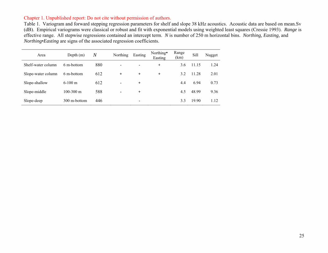
Chapter 1. Unpublished report: Do not cite without permission of authors. Table 1. Variogram and forward stepping regression parameters for shelf and slope 38 kHz acoustics. Acoustic data are based on mean.Sv (dB). Empirical variograms were classical or robust and fit with exponential models using weighted least squares (Cressie 1993). Range is effective range. All stepwise regressions contained an intercept term. N is number of 250 m horizontal bins. Northing, Easting, and Northing•Easting are signs of the associated regression coefficients.
Area Depth (m) N Northing Easting Northing• Easting
Range (km) Sill Nugget
Shelf-water column 6 m-bottom 880 - - + 3.6 11.15 1.24
Slope-water column 6 m-bottom 612 + + + 3.2 11.28 2.01
Slope-shallow 6-100 m 612 - + 4.4 6.94 0.73
Slope-middle 100-300 m 588 - + 4.5 48.99 9.36
Slope-deep 300 m-bottom 446 - 3.3 19.90 1.12
25

Chapter 1. Unpublished report: Do not cite without permission of authors. Table 2. Forward stepping regression results for slope acoustic and LIDAR observations. Acoustic data are based on lnABC and LIDAR data are based on untransformed backscatter. All stepwise regressions contained an intercept term. N is number of 250 m horizontal bins. Northing, Easting, and N•E (Northing•Easting) are signs of the associated regression coefficients.
38 kHz 6/10-6/12 Lidar 6/8 Lidar 6/11 Lidar 6/14
Depth (m) N Northing Easting N•E N Northing Easting N•E N Northing Easting N•E N Northing Easting N•E
2-6 564 - - + 537 - - + 530 + + +
6-12 611 + + + 564 - - + 537 - - + 530 + + +
12-18 611 + + + 564 - - 537 + 528 -
18-24 611 + 564 + 532 + + + 529
24-30 611 - - + 564 + 519 + + + 362
26

Chapter 1. Unpublished report: Do not cite without permission of authors. Table 3. Forward stepping regression parameters for shelf acoustic and LIDAR observations. Acoustic data are based on lnABC and LIDAR data are based on untransformed backscatter. All stepwise regressions contained an intercept term. N is number of 250 m horizontal bins. Northing, Easting, and N•E (Northing•Easting) are signs of the associated regression coefficients. 38 kHz 6/14-6/18 Lidar 6/13 Lidar 6/18 Lidar 6/19
Depth (m) N Northing Easting N•E N Northing Easting N•E N Northing Easting N•E N Northing Easting N•E
2-6 642 - - + 1047 - - + 943 + + +
6-12 885 + 641 - - + 1047 - - + 933 - +
12-18 885 - - + 640 + 1046 930 + + +
18-24 885 - - + 639 1030 + + + 909 + + +
24-30 884 - - + 485 + 221 145 -
27

Chapter 1. Unpublished report: Do not cite without permission of authors. Table 4. Variogram and forward stepping regression parameters for nighttime slope LIDAR. LIDAR data are based on untransformed backscatter. All stepwise regressions contained an intercept term. N is number of 250 m horizontal bins. Northing, Easting, and N•E (Northing•Easting) are signs of the associated regression coefficients*. Empirical variograms were robust and fit with exponential models using weighted least squares (Cressie 1993). Range is effective range. Lidar 6/13 night
Depth (m) N Northing Easting N•E Range (km) Sill Nugget
2-6 843 - - + 1.9 12.04 3.15
6-12 843 + + + 1.4 0.48 0.15
12-18 843 1.4 22.78 4.53
18-24 843 2.1 247.91 206.97
24-30 843 3.5 185.93 84.48
30-bottom
28

Chapter 1. Unpublished report: Do not cite without permission of authors. Table 5. Variogram parameters for slope acoustic and LIDAR observations. Acoustic data are based on lnABC and LIDAR data are based on untransformed backscatter. Empirical variograms were classical or robust and fit with exponential or spherical models using weighted least squares (Cressie 1993). N is number of 250 m horizontal bins. Range for exponential model is effective range. All variograms included a nugget. Unbounded (linear) variograms have “inf” ranges and sills.
38 kHz 6/10-6/12 Lidar 6/8 Lidar 6/11 Lidar 6/14
Depth (m) N Range
(km) Sill Nugget N Range (km) Sill Nugget N Range
(km) Sill Nugget N Range (km) Sill Nugget
2-6 564 11.0 7.75 0.03 537 5.2 0.21 0.07 530 6.1 0.36 0.32
6-12 611 5.6 0.50 0.08 564 6.6 0.33 0.04 537 7.1 0.05 0.04 530 11.8 0.33 0.12
12-18 611 2.6 0.49 0.65 564 2.6 2.68 0.65 537 1.6 0.76 0.00 528 3.0 0.02 0.01
18-24 611 2.5 0.53 0.00 564 2.3 9.58 1.36 532 27.0 0.07 0.02 529 3.7 0.01 0.00
24-30 611 2.4 0.55 0.01 564 2.3 13.62 2.28 519 56.8 0.03 0.00 362 4.0 0.1 0.05
29

Chapter 1. Unpublished report: Do not cite without permission of authors. Table 6. Variogram parameters for shelf acoustic and LIDAR observations. Acoustic data are based on lnABC and LIDAR data are based on untransformed backscatter. Empirical variograms were classical or robust and fit with exponential or spherical models using weighted least squares (Cressie 1993). N is number of 250 m horizontal bins. Range for exponential model is effective range. Unbounded (linear) variograms have “inf” ranges and sills. 38 kHz 6/14-6/18 Lidar 6/13 Lidar 6/18 Lidar 6/19
Depth (m) N Range
(km) Sill Nugget N Range (km) Sill Nugget N Range
(km) Sill Nugget N Range (km) Sill Nugget
2-6 642 6.5 1.60 0.19 1047 3.9 6.16 0.71 943 10.7 51.82 24.51
6-12 885 4.0 0.83 0.08 641 14.3 0.60 0.58 1047 3.1 2.56 0.44 933 3.9 3.00 0.50
12-18 885 3.9 0.54 0.00 640 9.3 0.20 0.19 1046 3.5 0.30 0.47 930 inf inf 16.54
18-24 885 3.2 0.43 0.02 639 inf 19.31 0.00 1030 2.3 16.44 8.36 909 10.6 39.56 20.42
24-30 884 2.7 0.45 0.01 485 inf 265.81 0.03 221 1.5 5.51 0.44 145 inf inf 55.51
30

Chapter 1. Unpublished report: Do not cite without permission of authors. Appendix 1. Midwater trawl results for aggregation characterization.
Scientific Name Common Name 1 2 3 4 5 6 7 8 9 10 11 12 13 14 15 16 17 18 19 20 Agonus acipenserinus Sturgeon poacher 1 1 2 1 Alepisaurus ferox Longnose lancetfish 1 1 Atherestes stomias Arrowtooth flounder 1 1 1 4 1 Bathylagus pacificus Slender blacksmelt 664 Chauliodus macouni Pacific viperfish 3 Clupea harengus pallasi Pacific herring 16 4 13 1 3 Coryphaeanoides leptolepis Ghostly grenadie r 1 Diaphus theta California headlightfish 4 268 190 1550 Gadus macrocephalus Pacific cod 1 Hemitripterus bolini Bigmouth sculpin 1 Lampanyctus jordani Brokenline lanternfish 4 205 79 Lepidopsetta polyxystra Northern rocksole 1 Leuroglossus schmidti Northern smoothtongue 2 2450 6082 48,930 56,699Lipolagus ochotensis Eared blacksmelt 8 16 Lumpenus sagitta Pacific snake prickleback 1 1 Lycodapus c.f. poecilus Variform eelpout 15 24 Melamphaes lugubris Highsnout melamphid 3 Nannobrachium regale Pinpoint lanternfish 1 Onchorhynchus gorbuscha Pink salmon 4 1 Onchorhynchus keta Chum salmon 1 1 1 9 Onchorhynchus nerka Sockeye Salmon 1 Petromyzon tridentata lamprey 1 16 2 6 Pleurogrammus monopterygius Atka mackerel 1 1 Protomyctophys thompsoni Bigeye lanternfish 80 63 40 Pseudobathylagus milleri Stout blacksmelt 79 Sebastes alutus Pacific ocean perch 1 81 Sigmops gracilis Slender fangjaw 5 Stenobrachius leucopsarus Northern lampfish 793 1265 4688 Stenobrachius nannochir Garnet lanternfish 1027 Tactostoma macropus Longnose dragonfish 3 Theragra chocogramma Walleye pollock 3 17 1 47 5 1 1 22 7 7 1142 24 4 286 10 1 7 Triglops metopias Alaskan sculpin 1 1 Berryteuthis magister Magistrate armhook squid 3 1 Gonatopsis borealis Boreopacific armhook squid 54 752 Unidentified squid Squid 2 54 477
Grand Total 17 17 7 35 84 63 14 8 1 206 25 8 139 1148 1539 140 3524 7272 53,032 63,865
31

Chapter 1. Unpublished report: Do not cite without permission of authors. Appendix 2. Total MultiNet catches by taxonomic groups for aggregation characterization.
TAXON 1 2 5 6 7 8 9 11 12 13 15 16 17 18 20
Bryozoa 64 640 64 128 64 32 64 64 120 128 32 Cephalopoda 1 11 11 3 6 5 8 3 5 8 24 6 1 1 Chaetognatha 912 832 1312 320 1216 404 536 1280 256 2240 1152 140 2528 2528 929 Cirripeda 576 96 64 264 12 16 256 384 64 144 36 320 20 Cnidaria 276 56 538 81 97 129 45 360 109 291 221 304 112 92 42 Ctenophora 2 Cumacea 1 Decapoda 5394 1935 813 3881 9941 97 232 1144 461 2031 597 229 239 633 402 Echinodermata 32 32 64 8 64 Gammarida 8 1 1 Hyperiidea 448 3144 1425 1280 584 81 589 1041 388 694 2140 108 258 1996 154 Larvacea 1600 3280 2368 960 2944 536 112 4352 2880 2880 480 2120 1712 2688 864 Mollusca 4480 4296 1856 7132 5392 1368 337 7984 3292 4068 2380 1364 620 3880 1016 Ostracoda 16 464 229 96 Phoronida 128 Pisces 82 176 175 72 128 63 39 80 98 78 103 22 29 200 40 Polychaeta 1 8 9 9 2 1 341 1 20 13 19 127 153 38 Tunicata 4 2 4 6 4 Total 13270 14954 8671 13921 20582 2793 1947 16841 7974 12518 7244 4582 6131 12849 3699
32

Chapter 1. Unpublished report: Do not cite without permission of authors.
33
Figure 1. Survey location showing systematic transects.
0.40 0.42 0.44 0.46
5.98
6.00
6.02
Easting (m*10^6)
Nor
thin
g (m
*10^
6)

Chapter 1. Unpublished report: Do not cite without permission of authors.
Figure 2. Geostatistical predictions of Sv_mean for shelf and slope-water-column sampling areas.
0.40 0.42 0.44 0.46
BSea Sv Predictions OS.wc and NS with Trend
Easting (m*10^6)
5.98
5.99
6.00
6.01
6.02
Nor
thin
g (m
*10^
6)
-83-76-69-62-55
34

Chapter 1. Unpublished report: Do not cite without permission of authors.
Figure 3. Geostatistical predictions of Sv_mean in slope-shallow (A), slope-middle (B), and slope-deep
(C) depth layers.
6-100 m
BSea OS Sv.mean for layers
100-300 m
300 m-bottom
0.40 0.42 0.44 0.46Easting (m*10^6)
5.98
5.99
6.00
6.01
6.02
Nor
thin
g (m
*10^
6)
-94-89-84-79-74-69-64-59-54-49
35

Chapter 1. Unpublished report: Do not cite without permission of authors.
Figure 4. Agglomerative hierarchical cluster analysis results for (A) slope and (B) shelf regions. Numbers
indicate depth layer (1: 6-12 m, 2: 12-18 m, 3: 18-24 m, 4: 24-30 m). In slope, circles are acoustic (10-12
June) and LIDAR are squares (8 June), triangles (11 June), and diamonds (14 June). In shelf, circles are
acoustic (14-18 June) and LIDAR are squares (13 June), triangles (18 June), and diamonds (19 June).
17 18 19 20 2122 23 2425 26
27
28 29
30
31
32
02
46
Hei
ght
1
2
3 45
6
7 8
9 10
11
12
13
14 15 16
02
46
Hei
ght
Shelf
Slope
1 4 3 2 1 2 3 4
2
3
4
11 2
3
4
1 4 3
2
1
2
3 4
2 3 4
1
1 2
3
4
36

Chapter 1. Unpublished report: Do not cite without permission of authors.
Figure 5. Representative examples of target assemblages observed on the echosounder and sampled with
midwater trawl or MultiNet. Pelagic layers (A, ID11; B, ID 17), demersal school (C, ID 16), scattered
pelagics (D, ID 14), and schools (E, ID3; F, ID 12).
37

Chapter 1. Unpublished report: Do not cite without permission of authors.
Figure 6. Species distribution within target assemblages in the shelf region from midwater trawl (A) and
MultiNet (B) samples. Equilibrium trawl depth increases from left to right.
0
25
50
75
1 2 3 4 5 6 7
flat herring other pollock
0
250
500
750
1000
1 2 n/a n/a 5 6 7
Cope Deca Euph Amph Moll
38
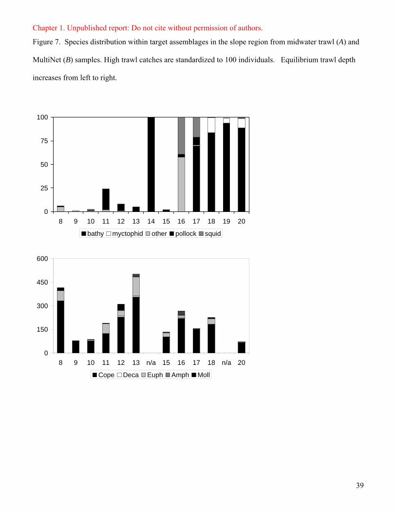
Chapter 1. Unpublished report: Do not cite without permission of authors.
Figure 7. Species distribution within target assemblages in the slope region from midwater trawl (A) and
MultiNet (B) samples. High trawl catches are standardized to 100 individuals. Equilibrium trawl depth
increases from left to right.
0
25
50
75
100
8 9 10 11 12 13 14 15 16 17 18 19 20
bathy myctophid other pollock squid
0
150
300
450
600
8 9 10 11 12 13 n/a 15 16 17 18 n/a 20
Cope Deca Euph Amph Moll
39

Chapter 2. Unpublished report: Do not cite without permission of authors.
Forage Fish in Shallow Nearshore Habitats of the Bering Sea
John F. Thedinga, Scott W. Johnson, Mandy R. Lindeberg, and A. Darcie Neff NOAA, Auke Bay Laboratory, Juneau, AK 99801
Abstract
Nearshore waters of the Bering Sea provide habitat for several forage fish species that are
important in the diet of marine mammals, seabirds, and other fishes. Shallow, nearshore waters
(<5 m deep, <20 m from shore) of the Bering Sea were sampled with a beach seine to estimate
forage fish distribution and relative abundance in June 2005. Three habitat types were sampled:
non-vegetated sand substrate, vegetated cobble substrate, and vegetated bedrock substrate. A
total of 70 sites were seined on Akutan, Akun, and Unalaska Islands. Total catch was 83,910 fish
representing 27 species. Catch per seine haul (all spp.) varied from no fish to over 15,000 fish.
Pacific sand lance was the dominant forage fish species captured—approximately 35,000 fish
(42% of total catch) occurring in 60% of all seine hauls. Mean size of sand lance captured was
106 mm fork length (FL). Other commonly captured forage fish were young-of-the-year (YOY)
Pacific sandfish (mean FL = 36 mm) and YOY gadids (mean FL = 31 mm). Fish were
distributed unequally among habitats. Mean catch per seine haul of all species was 1,647 fish in
vegetated cobble sites, 1,170 fish in non-vegetated sand sites, and 79 fish in vegetated bedrock
sites. Most sand lance (98%) were captured in non-vegetated sand sites, and most sandfish (96%)
and gadids (97%) were captured in vegetated cobble substrate sites. Although we captured
several forage fish species in shallow, nearshore waters in June, use of the nearshore by forage
fish in other seasons and other areas of the Bering Sea is largely unknown. Beach seining is an
effective method for sampling forage fish, particularily sand lance, in the nearshore of the Bering
Sea.
1

Chapter 2. Unpublished report: Do not cite without permission of authors.
Introduction
Forage fish assemblages in the shallow, nearshore waters (<5 m deep, <20 m from shore)
of the Bering Sea have been examined in only a few locations. In the western Bering Sea,
Isakson et al. (1971) described the nearshore fish community at Amchitka Island. In the
southeastern Bering Sea, Houghton (1987) examined nearshore fish assemblages, and Warner
and Shafford (1981) surveyed spawning forage fish. In Port Moller, McGurk and Warburton
(1992) studied the life history of Pacific sand lance (Ammodytes hexapterus). The only studies of
nearshore fish within our study area were limited beach seine surveys by Robards (1999) and
Robards and Shroeder (2000) in Unalaska Bay and Akutan Bay.
Nearshore areas provide important habitat for many fish species and are vulnerable to
human disturbance from oil and other shoreline development. Nearshore habitat is of particular
importance to juvenile stages of Pacific cod (Gadus macrocephalus), walleye pollock (Theragra
chalcogramma), and many flatfish and rockfish species, providing young-of-the-year (YOY) fish
with essential nursery habitat. Forage fish such as Pacific sand lance, Pacific sandfish (Trichodon
trichodon), and Pacific herring (Clupea pallasii) use nearshore areas for spawning and rearing,
but the location, timing, and extent of these activities in the nearshore of the Bering Sea is poorly
understood.
The Bering Sea supports the world’s largest walleye pollock fishery in addition to
important Pacific cod, Pacific halibut (Hippoglossus stenolepis), and king crab (Paralithodes
spp.) fisheries. Additionally, the area supports large populations of marine mammals and
seabirds. Forage fish play an important part in the Bering Sea ecosystem because of their role as
food for higher trophic level predators. Pacific sandfish occurred in up to 64% of Steller sea lion
(Eumetopias jubatus) scats in the Aleutian Islands (Sinclair and Zeppelin 2002). Sand lance
(Ammodytes spp.) are possibly the single most important taxon of forage fish in the northern
hemisphere (Springer and Speckman 1997), and are a major prey species for at least 40 species
of birds, 12 species of marine mammals, and 45 species of fish (Field 1988; Willson et al. 1999).
Our objective was to examine forage fish assemblages in several nearshore habitats in the Bering
Sea in the vicinity of Unalaska, Alaska.
2

Chapter 2. Unpublished report: Do not cite without permission of authors.
Methods
Study locations
Fishes were sampled with a beach seine in the shallow, nearshore waters (<5 m deep, <20
m from shore) of the Bering Sea from June 10-18, 2005. A total of 70 sites were sampled on
Akutan, Akun, and Unalaska Islands (Fig.1). Different habitat types were sampled to account for
segregation of some fish species based on habitat preference (Johnson et al. 2003). Habitat types
included sand substrate (33 sites) with little or no rooted vegetation, cobble substrate (27 sites)
with understory kelps dominated by Alaria marginata and Laminaria longipes, and steep
bedrock walls (10 sites) with understory kelps dominated by A. marginata and Cymathere
triplicata.
Fish capture and habitat
Fish were captured with a 37-m variable-mesh beach seine that tapered from 5 m wide at
the center to 1 m wide at the ends. Outer panels were each 10 m of 32-mm stretch mesh,
intermediate panels were each 4 m of 6-mm square mesh, and the bunt was 9 m of 3.2-mm
square mesh. We set the seine as a Around haul@ by holding one end on the beach, backing around
in a skiff with the other end to the beach about 18 m from the starting point, and pulling the seine
onto shore. The seine had a lead line and a float line so that the bottom contacted the substratum
and the top floated on the surface. Sites were sampled during daylight independent of tide height.
Fish captured with the seine were identified to species and enumerated. For large catches,
the number of fish was estimated gravimetrically. A random subsample of approximately 500
fish was removed from the total catch, and the remaining fish were collectively weighed to the
nearest 0.1 kg. Fish in the subsample were weighed to the nearest gram and counted by species.
A mean weight of fish determined from the subsample was used to estimate the number of fish in
the total catch. The proportion of each species in the subsample was also used to determine the
species composition of the total catch. Fork length (FL) was measured to the nearest millimeter
for up to 50 individuals for most species. The number of larvae (≤ 30 mm) in large catches was
visually estimated.
Habitat of the areas seined (subtidal) was classified at each site, and the adjacent
intertidal areas were classified at about one half of the sites. For the subtidal areas, water
temperature and salinity (practical salinity scale; PSS) were measured at a depth of 20 cm with a
thermometer and a hand-held refractometer. Substrate composition was visually estimated and
3

Chapter 2. Unpublished report: Do not cite without permission of authors.
vegetation was identified. For the intertidal areas, ShoreZone survey methods were used (Howes
and Berry 2001).
Data analysis
We used one-way ANOVA to test for significant differences in catch among habitat types
and the Tukey test for pairwise tests among habitat types. Kruskal-Wallis ANOVA was used to
test for significant differences in the Shannon-Weaver diversity index (H′) among habitat
types—pairwise comparisons were tested with Dunn’s method.
Results
Catch
A total of 83,910 fish representing 27 species were captured at 70 sites. Catches varied
from no fish to more than 15,000 fish per seine haul. Pacific sand lance was the dominant fish
species captured—approximately 35,000 were captured, and they occurred in 60% of hauls.
Three species, Pacific sand lance, pink salmon (Oncorhynchus gorbuscha), and Pacific sandfish,
and one family of fishes, Gadidae, comprised 95% of the total catch.
Habitat
Fish were distributed unequally among habitats (Table 1). Catch per seine haul for all
species was significantly greater (P = 0.001) in cobble sites than bedrock sites and significantly
greater (P = 0.040) in sand sites than bedrock sites. Mean catch per seine haul for all species was
1,647 fish in cobble sites, 1,171 fish in sand sites, and 79 fish in bedrock sites. Most Pacific sand
lance (98%) were captured in sand sites, whereas most gadids (97%), pink salmon (80%), and
Pacific sandfish (96%) were captured in cobble sites. In sand sites, sand lance was the dominant
species captured (mean = 1,056 fish per haul), occurring in 94% of sites and comprising 90% of
the catch. Young-of-the-year sandfish were the second most abundant forage fish in sand sites
(mean = 11 fish per haul), occurring in 24% of sites and comprising 1% of the catch. In cobble
sites, YOY gadids were the dominant fish captured (mean = 755 fish per haul), occurring in 74%
of sites and comprising 46% of the catch. Sandfish were the second most abundant forage fish in
cobble sites (mean = 373 fish per haul), occurring in 48% of sites and comprising 23% of the
catch. Sand lance were captured in one third of cobble sites but mean catch was only 22 fish per
haul. In bedrock sites, YOY gadids (mean = 34 fish per haul) and pink salmon fry (mean = 34
fish per haul) were the dominant fish captured, occurring in 70% and 30% of hauls, and
4

Chapter 2. Unpublished report: Do not cite without permission of authors.
comprising a total of 69% of the catch. Few sand lance (mean = 0.2 fish per haul) and sandfish
(mean = 3 fish per haul) were captured in bedrock sites.
Species richness varied by habitat. The fewest number of species (16) were captured at
bedrock sites, whereas more species were captured at sand (23) and cobble (27) sites. The
Shannon-Weaver diversity index (H′) was significantly different (P = 0.007) among the three
habitat types. Pairwise comparisons showed significant differences (P<0.05) between bedrock
and cobble sites and between bedrock and sand sites. Dominance by Pacific sand lance in sand
habitat (90% of catch; Table 1) reduced the diversity index for sand habitat.
Fish length and age
Most captured fish were juveniles. Mean FL of all fish ranged from 23 mm to 408 mm.
Length frequencies of Pacific sand lance indicated 2 or 3 age groups with modes of 60-69 mm
and 120-129 mm (Fig 2). All Pacific sandfish, pink salmon, and gadids were YOY (Table 2).
Discussion
There has been little research on nearshore forage fish communities in the Bering Sea.
Forage fish life histories, except for Pacific herring are poorly understood, primarily because
there are no commercial fisheries for most forage fish species. Our study showed that nearshore
fish assemblages on Akutan, Akun, and Unalaska Islands were dominated by forage fish,
particularly Pacific sand lance. In nearshore waters of other areas of the Bering Sea, Houghton
(1987) reported that the most abundant fish in beach seine catches from late June to mid
September from False Pass to Ugashik Bay was Pacific sand lance. McGurk and Warburton
(1992) found that larvae from sand lance that spawned in Port Moller in the southeastern Bering
Sea reared in the same or nearby estuarine habitats. In areas near our sampling sites in Unalaska
Bay and Akutan Harbor, however, Robards (1999) and Robards and Schroeder (2000) reported
beach seine catches in summer were dominated by pink salmon fry, and captured few sand lance.
Mean catch per seine haul by Robards and Robards and Schroeder (653 and 536 fish per haul)
were about half of our catch (1,202 fish per haul). We did not capture any Pacific herring,
capelin (Mallotus villosus) or other smelts (Osmeridae).
Fish catch and species richness varied by habitat. Although we captured Pacific sand
lance in all habitats, highest catches were in sand habitat. In most studies in the Bering Sea,
catches of forage fish were not separated by habitat type (Houghton1987; Robards 1999;
5

Chapter 2. Unpublished report: Do not cite without permission of authors.
Robards and Schroeder 2000). Isakson et al. (1971) divided their nearshore sampling areas near
Amchitka Island into rock/algae and sand/gravel habitats and found different fish communities in
each habitat—Pacific sand lance and Pacific sandfish were prominent species in sand/gravel
habitat but not in rock/algae habitat. In our study, 96% of sandfish were captured in cobble
habitat, whereas in southeastern Alaska, most sandfish were captured in bedrock habitat
(Thedinga et al. in press).
Most of the forage fish we captured were juveniles. In other areas of Alaska, most forage
fish captured with beach seines were also juveniles (Abookire et al. 2000; Robards 2000;
Johnson et al. 2005; Thedinga et al. in 2006; Thedinga et al. in press; Johnson et al. in prep.).
Some adult forage fish spawn in the shallow nearshore (McGurk and Warburton 1992; Warner
and Shafford 1981), but timing and habitats used for spawning are poorly understood.
Conclusions
Shallow, nearshore areas in the Bering Sea provide rearing habitat for several species of
forage fish, most importantly Pacific sand lance. How long sand lance and YOY Pacific sandfish
and gadids rear in the nearshore is unknown, although Houghton (1987) captured sand lance
throughout summer in the nearshore of the eastern Bering Sea, and McGurk and Warburton
(1992) captured sand lance larvae throughout summer in Port Moller. In southeastern Alaska,
Sand lance and sandfish were caught throughout summer (Johnson et al., 2003; Johnson and
Thedinga, 2005; Thedinga et al. in 2006; Thedinga et al. in prep.), but few were captured in
winter (Thedinga et al. in 2006; Thedinga et al. in prep.).
Seasonal studies would help define temporal use of shallow nearshore habitats in the
Bering Sea by sand lance and other forage fish species (e.g., Pacific herring, capelin). Pacific
herring, capelin, sand lance, and Pacific sandfish spawn in the nearshore (Marliave 1980; Warner
and Shafford 1981; McGurk and Warburton 1992), but we do not fully understand their
dependence and fidelity to the different habitats types within the nearshore, or which habitats are
more important for different life stages. Nearshore waters are some of most productive areas in
Alaska and are vulnerable to changing environmental perturbations and increasing stress from
shoreline development from oil and other shoreline development. In particular, information is
needed on the function and use of nearshore habitats by forage fish because of their importance
as a prey resource for higher-level-trophic consumers (e.g., marine mammals, fish). A better
6

Chapter 2. Unpublished report: Do not cite without permission of authors.
understanding of how the nearshore environment supports ecologically important forage fish
species will help managers conserve forage fish populations and protect essential habitats.
Literature cited
Abookire, A.A., J.F. Piatt, and M.D. Robards. 2000. Nearshore fish distributions in an Alaskan
estuary in relation to stratification, temperature and salinity. Est. Coast. Shelf Sci. 51:45-
59.
Field, L.J. 1988. Pacific sand lance, Ammodytes hexapterus, with notes on related Ammodytes
species. In: Wilimovsky, N. J., Incze, L. S., Westrheim, S. J. (Eds.), Species Synopses,
Life Histories of Selected Fish and Shellfish of the Northeast Pacific and Bering Sea.
Available from Washington Sea Grant Program, 3716 Brooklyn Ave., NE, Seattle, WA,
pp. 15–33.
Houghton, J.P. 1987. Forage fish use of inshore habitats north of the Alaska Peninsula. In:
Forage fishes of the southeastern Bering Sea Conference proceedings. MMS 87-0017.
Howes, D., and H. Berry. 2001. British Columbia biophysical Shore-Zone mapping system. A
systematic approach to characterize coastal habitats in the Pacific Northwest. Puget
Sound Research Conference, Seattle, Washington, 11 p.
Isakson, J.S., C.A. Simenstad, and R.L. Burgner. 1971. Fish communities and food chains in the
Amchitka area. BioScience 21:666–670.
Johnson, S.W., M.L. Murphy, D.J. Csepp, P.M. Harris, and J.F. Thedinga. 2003. A survey of fish
assemblages in eelgrass and kelp habitats of southeastern Alaska. U.S. Dep. Commer.,
NOAA Tech. Memo. NMFS-AFSC-139, 39 p.
Johnson, S.W., A.D. Neff, and J.F. Thedinga. 2005. An atlas on the distribution and habitat of
common fishes in shallow nearshore waters of southeastern Alaska. U.S. Dep. Commer.,
NOAA Tech. Memo. NMFS-AFSC-139, 89 p.
7

Chapter 2. Unpublished report: Do not cite without permission of authors.
Johnson, S.W., J.F. Thedinga, and K.M. Munk. In prep. Habitat, age, and diet of an important
forage fish in southeastern Alaska: Pacific sand lance, Ammodytes hexapterus.
Marliave, J.B. 1980. Spawn and larvae of the Pacific sandfish, Trichodon trichodon. Fish. Bull.
78:959-964.
McGurk, M.D. and H.D. Warburton. 1992. Pacific sand lance of the Port Moller estuary,
southeastern Bering Sea: an estuarine-dependent early life history. Fish. Oceanogr. 1:4,
306-320.
Robards, M. 1999. Assessment of nearshore fish around Unalaska using beach seines during July
1999. Final report. USGS Biological Resources Division, Alaska Biological Sciences
Center, Anchorage, AK.
Robards, M. and M. Schroeder. 2000. Assessment of nearshore fish around Akutan Harbor using
beach seines during March and June 2000. Final report. USGS Biological Resources
Division, Alaska Biological Sciences Center, Anchorage, AK.
Sinclair, E.H., and T.K. Zeppelin. 2002. Seasonal and spatial differences in diet in the western
stock of Steller sea lions (Eumetopias jubatus). J. Mamm. 83:973B990.
Springer, A.M., Speckman, S.G., 1997. A forage fish is what? Summary of the Symposium. In:
Forage Fishes in Marine Ecosystems. Proceedings of the International Symposium on the
Role of Forage Fishes in Marine Ecosystems. Alaska Sea Grant College Program Report
No. 97-01. University of Alaska, Fairbanks, AK, pp. 773–805.
Thedinga, J.F., and S.W. Johnson. In press. Habitat, age, and diet of a forage fish in southeastern
Alaska: Pacific sandfish (Trichodon trichodon). Fisheries Bulletin.
8

Chapter 2. Unpublished report: Do not cite without permission of authors.
Thedinga, J.F., S.W. Johnson, and D.J. Csepp. 2006. Nearshore fish assemblages in the vicinity
of two Steller sea lion haulouts in southeastern Alaska. In: Sea Lions of the World.
Alaska Sea Grant College Program Report No. AK-SG-06-01. University of Alaska,
Fairbanks, AK, pp. 269-284.
Warner, I.M. and P. Shafford. 1981. Forage fish spawning surveys – southern Bering Sea. In
Environmental assessment of the Alaskan continental shelf, Final report. Vol. 10:64 p.
Willson, M.F., Armstrong, R.H., Robards, M.D., and Piatt, J.F., 1999. Sand lance as cornerstone
prey for predator populations. In: Robards, M. D., Willson, M. F., Armstrong, R. H.,
Piatt, J. F. (Eds.), Sand lance: a Review of Biology and Predator Relations and Annotated
Bibliography. Research paper PNW-RP-521. U.S. Department of Agriculture, Forest
Service, Pacific Northwest Research Station, Portland, OR, pp. 17–44.
9

Chapter 2. Unpublished report: Do not cite without permission of authors.
Table 1. Catch per haul and frequency of occurrence (%) of fish captured with a beach seine in
three habitat types in the Bering Sea, on Akutan, Akun, and Unalaska Islands, Alaska, June
2005. A blank represents the absence of a species from a site. N = 10 hauls in bedrock sites, 27
hauls in cobble sites, and 33 hauls in sand sites. Bedrock Cobble Sand Common name Scientific name Catch/haul %
l
Catch/haul % Catch/haul % Pacific sand lance Ammodytes hexapterus 0.2 20.0 21.8 33.3 1,056.4 93.9Juvenile gadid Gadidae 34.0 70.0 755.1 74.1 6.3 18.2Pink salmon Oncorhynchus gorbuscha 34.1 30.0 379.1 63.0 66.4 48.5Pacific sandfish Trichodon trichodon 3.4 30.0 373.4 48.1 11.0 24.2Snake prickleback Lumpenus sagitta 87.0 11.1 0.8 3.0Juvenile cottid Cottidae 1.4 30.0 12.4 81.5 12.5 30.3Silverspotted sculpin Blepsias cirrhosus 2.5 50.0 6.0 66.7 Rock sole Lepidopsetta spp. 1.0 14.8 4.6 54.5Juvenile flatfish Pleuronectidae 0.1 10.0 1.1 22.2 4.2 39.4Chum salmon Oncorhynchus keta 3.2 3.7 0.4 3.0Dolly Varden Salvelinus malma 0.3 14.8 2.8 30.3Rock greenling Hexagrammos lagocephalus 0.4 30.0 2.8 66.7 0.1 6.1Coho salmon Oncorhynchus kisutch 0.3 3.7 1.7 9.1Frog sculpin Myoxocephalus stelleri 0.1 10.0 0.4 18.5 1.3 39.4Sturgeon poacher Podothecus accipenserinus 1.5 9.1Juvenile greenling Hexagrammidae 0.9 29.6 <0.1 3.0Pacific cod Gadus macrocephalus 0.9 3.7 Starry flounder Platichthys stellatus <0.1 3.7 0.7 27.3Juvenile snailfish Liparidae 0.1 10.0 0.7 18.5 Manacled sculpin Synchirus gilli 1.9 20.0 Masked greenling Hexagrammos octogrammus 0.1 10.0 0.3 14.8 0.2 6.1Red Irish lord Hemilepidotus hemilepidotus 0.1 10.0 0.2 14.8 Black rockfish Sebastes melanops 0.2 14.8 Juvenile poacher Agonidae 0.2 12.1Crescent gunnel Pholis laeta 0.1 11.1 Sockeye salmon Oncorhynchus nerka 0.1 3.0Threespine stickleback Gasterosteus aculeatus 0.1 10.0 <0.1 3.7 Armorhead sculpin Gymnocanthus galeatus 0.1 3.7 Great sculpin Myoxocephalus polyacanthocephalus 0.1 6.1Kelp greenling Hexagrammos decagrammus 0.1 10.0 <0.1 3.7 Alaska plaice Pleuronectes quadrituberculatus <0.1 3.0English sole Parophrys vetulus <0.1 3.0Dusky rockfish Sebastes ciliatus <0.1 3.7
10

Chapter 2. Unpublished report: Do not cite without permission of authors.
Table 2. Total catch, mean fork length, and range of fish captured with a beach seine in the
Bering Sea, on Akutan, Akun, and Unalaska Islands, Alaska, June 2005. Sample
locations are shown in Figure 1.
Total Number Fork length (mm) Family or Species Catch Measured Mean Range Pacific sand lance 35,451 1,109 106 035-190 Gadidae 20,934 451 23 15-31 Pink salmon 12,770 615 45 30-65 Pacific sandfish 10,478 299 36 17-56 Snake prickleback 2,374 92 122 037-320 Cottidae 761 6 30 16-49 Silverspotted sculpin 186 24 76 019-144 Rock sole 179 167 181 032-522 Pleuronectidae 168 36 39 16-63 Chum salmon 100 22 63 56-71 Dolly Varden 99 99 307 130-535 Rock greenling 81 77 258 120-495 Coho salmon 64 39 121 035-145 Frog sculpin 53 48 384 080-485 Sturgeon poacher 51 5 55 25-97 Hexagrammidae 24 16 54 48-65 Pacific cod 23 13 200 178-237 Starry flounder 23 13 372 300-520 Liparidae 21 14 25 12-78 Manacled sculpin 19 4 36 18-55 Masked greenling 14 14 288 131-480 Red Irish lord 7 6 252 087-378 Black rockfish 6 6 120 092-160 Sockeye salmon 3 3 66 62-73 Threespine stickleback 2 2 69 65-73 Armorhead sculpin 2 2 78 70-85 Great sculpin 2 2 408 400-415 Kelp greenling 2 2 373 345-400 Alaska plaice 1 1 185 -- Dusky rockfish 1 1 90 -- English sole 1 1 116 -- Other species 10 0 -- --
11

Chapter 2. Unpublished report: Do not cite without permission of authors.
Figure 1. Location of nearshore sites sampled with a beach seine in the Bering Sea on Akutan,
Akun, and Unalaska Islands, Alaska, June 2005.
Akun Island
12

Chapter 2. Unpublished report: Do not cite without permission of authors.
Figure 2. Length frequencies of Pacific sand lance (Ammodytes hexapterus) captured with a
beach seine in nearshore habitats of the Bering Sea on Akutan, Akun, and Unalaska
Islands, Alaska, June 2005.
0
2
4
6
8
10
12
14
16
18
20
40-49
50-59
60-69
70-79
80-89
90-99
100-1
09
110-1
19
120-1
29
130-1
39
140-1
49
150-1
59
160-1
69
170-1
79
180-1
89
190-1
99
Fork length (mm)
Freq
uenc
y (%
)
0
2
4
6
8
10
12
14
16
18
20
0
2
4
6
8
10
12
14
16
18
20
40-49
50-59
60-69
70-79
80-89
90-99
100-1
09
110-1
19
120-1
29
130-1
39
140-1
49
150-1
59
160-1
69
170-1
79
180-1
89
190-1
9940
-4950
-5960
-6970
-7980
-8990
-99
100-1
09
110-1
19
120-1
29
130-1
39
140-1
49
150-1
59
160-1
69
170-1
79
180-1
89
190-1
99
Fork length (mm)
Freq
uenc
y (%
)
13

Chapter 3. Unpublished report: Do not cite without permission of authors.
Distribution, composition and energy density of zooplankton in the southeastern Bering Sea
Nicola Hillgruber1, Johanna J. Vollenweider2, Wyatt Fournier21School of Fisheries and Ocean Science, University of Alaska Fairbanks, Juneau, AK 99801
2NOAA, NMFS, Auke Bay Laboratory, Juneau, AK 99801
Abstract
The southeastern Bering Sea is a productive area that supports an abundance of
economically valuable and ecologically important vertebrate and invertebrate taxa. As part of a
survey directed at investigating assessment methods for forage taxa in the southeastern Bering
Sea, here we describe the distribution, density, and energy content of zooplankton and
micronekton taxa north of Akutan and Akun Island in June 2005. CTD casts and depth-stratified
zooplankton sampling were conducted on stations ranging from nearshore areas (< 100 m) to the
continental shelf break.
The dominant zooplankton taxa were copepods, followed by euphausiids (Euphausia
pacifica, Thyssanoessa inermis, T. longipes, T. spinifera, Tessarabrachion oculatum), pteropods
(Clione limacina, Limacina helicina), larvaceans (Oikopleura sp.), hyperiid amphipods
(primarily Parthemisto pacifica), and chaetognaths (Sagitta sp.). The major copepod taxa were a
mixture of oceanic (Neocalanus spp., Eucalanus bungii, Metridia pacfica) and neritic
(Pseudocalanus spp., Calanus marshallae, and Acartia longiremis) species. Zooplankton density
in the upper 100 m of the water column was significantly higher in the nearshore waters. This
difference in density was largely caused by significantly higher densities of copepods, namely A.
longiremis, C. marshallae, and Pseudocalanus spp. in the nearshore waters. The oceanic
copepod M. pacifica appeared to be more abundant in the slope waters. On a relative mass basis
(kJ g-1 dry mass), the 2 species of pteropods had the most disparate energy contents amongst all
the species analyzed, C. limacina having the greatest energy content and L. helicina having the
least. Copepods were relatively high in energy content, followed by chaetognaths, euphausiids
and hyperiid amphipods. Though copepods, and secondarily euphausiids, were the most
abundant taxa, euphausiids provided the most energy available to predators due to their large
size. In addition, chaetognaths were a large energy source, despite low densities.
Our results indicate that the nearshore habitat was more productive than offshore waters
as was evidenced by relatively greater zooplankton abundance and total energy content.
1

Chapter 3. Unpublished report: Do not cite without permission of authors.
Introduction
The southeastern Bering Sea is a productive area that supports an abundance of
economically valuable and ecologically important vertebrate and invertebrate taxa (NRC 1996).
In recent years, climate shifts and resultant changes in the meteorological forcing have been
implicated in the transformation of the Bering Sea ecosystem (Napp & Hunt 2001, Coyle &
Pinchuk 2002, Hunt et al. 2002, Napp et al. 2002). Responses of the Bering Sea and the North
Pacific ecosystem to these climatic variations are apparent in changes in species abundance and
composition, e.g., declines in the abundance of seabirds, Steller sea lions (Eumetopias jubatus)
and forage species (Merrick et al. 1997, Anderson & Piatt 1999). It is the latter group of taxa in
particular that is currently still difficult to estimate in their abundance due to their generally
ephemeral and patchily concentrated distribution. However, it is also these taxa that are of
primary importance to the Bering Sea ecosystem, because they effectively link primary and
secondary consumers to higher trophic level fishes, seabirds and marine mammal species. Lack
of data on forage species abundance, distribution, and life history patterns currently limits our
understanding of the role of forage species in the Bering Sea ecosystem. However, it this
information that is of exceptional importance to improve our understanding of those processes
involved in changing the composition of the Bering Sea ecosystem and to advance predictions
about the future of top predators such as sea birds, marine mammals and piscivorous fishes.
Changes in the Bering Sea climate will directly affect all marine taxa through variations
in sea temperature. However, climatologic changes can also indirectly impact higher trophic
levels through trophic pathways (e.g., Hunt et al. 2002). Thus, not only differences in
zooplankton abundance and distribution may be responsible for growth and survival of
planktivorous forage species, but also variations in energy density of the given planktonic prey
taxa may result in increased or decreased condition as well as survival probability of the
consumer (Foy and Norcross 1999).
The zooplankton and micronekton communities consist of very diverse taxa that are
likely to react vastly differently to climatic changes. A community-specific reaction to climate
forcing has been shown in the western North Pacific (Chiba et al. 2006), where responses of taxa
varied based on their seasonal patterns of peak abundance; e.g., spring-summer copepod
communities, which were dominated by cold water species, showed a shift in their seasonal peak
abundance by one month as a result of an anomalous predominance of fresh, cold surface water
2

Chapter 3. Unpublished report: Do not cite without permission of authors.
during winter-spring in the 1970 (Chiba et al. 2006). Similar taxa-specific responses have been
observed in the Bering Sea (e.g., Brodeur et al. 1999, Napp & Hunt 2001, Napp et al. 2001,
Stockwell et al. 2001, Coyle & Pinchuk 2002, Napp et al. 2002). The Oscillating Control
Hypothesis (OCH) proposes a mechanism for the pelagic ecosystem of the southeastern Bering
Sea to be impacted by either bottom-up or top-down processes depending on climatic patterns
(Hunt et al. 2002). During the current warm regime of the Bering Sea, top-down control of
piscivorous fishes will not only limit the abundance of forage fishes, but at the same time, by
removing the predation pressure on zooplankton, increase the abundance of other planktivores,
e.g., jellyfish and chaetognaths. The complexity of these species-specific responses of the
pelagic ecosystem to climatic changes makes it apparent that a better knowledge of the
southeastern Bering Sea zooplankton and micronekton communities is essential in order to
understand and predict changes in this ecosystem.
In addition to measures of zooplankton abundance and distribution, the ability to predict
climate change effects on forage fish populations and consequently higher trophic levels is
significantly enhanced with the incorporation of quantitative energy pathways. Abundance
estimates of multiple trophic levels alone fail to account for discrepancies in energy content
amongst prey species. Incorporation of species variation in energy content can reveal
significantly different sources of dietary energy than would otherwise be indicated by measures
of biomass consumed alone (Vollenweider et al. 2006). Thus, the combination of zooplankton
energy content and abundance elucidate energy availability which may influence the structure of
energy pathways beyond what is expected from abundance data alone.
Energy availability of from prey influences organism fitness and consequently exerts
control on population and food web structure. Juvenile forage fish in particular, are highly
susceptible to energy limitation, particularly at high latitudes such as the North Pacific Ocean
(Foy and Norcross 1999). Juveniles must balance energy allocation between the demands of 1)
growth for predation avoidance, and 2) energy storage to forestall starvation during periods of
limited resource. If minimum threshold levels of storage energy are not attained during spring
and summer plankton blooms, juveniles suffer predation or starvation mortalities resulting in
poor year-class strength (Paul and Paul 1998). Similarly, energy limitations for mature fish can
structure forage fish populations by limiting the amount of energy available for gonad
provisioning and other reproductive costs (Robards 1999). Despite the importance of
3

Chapter 3. Unpublished report: Do not cite without permission of authors.
zooplankton energy values which are essentially the foundation of bottom-up structure, little data
exists for the North Pacific Ocean (Musayeva and Sokolova 1979).
As part of a study examining different methods for assessment of Bering Sea forage
species abundance, we analyzed distribution and abundance of zooplankton and micronekton
prey taxa and their energy density. To our knowledge, this is the first study to compare
distributional and energetic patterns of selected zooplankton and micronekton taxa from the
southeastern Bering Sea. Specifically, our objectives were:
1. Examine zooplankton and micronekton species composition and abundance in the
nearshore and offshore waters off Akutan and Akun Island in the southeastern Bering
Sea.
2. Analyze and compare energy density major zooplankton and micronekton taxa.
3. Estimate the total energy density of zooplankton and micronekton biomass in our study
area.
Methods
Study area
This study was conducted in the southeastern Bering Sea, north of the Aleutian Islands.
The Aleutians, a chain of volcanic islands, form a boundary between the North Pacific Ocean
and the Bering Sea. This boundary, however, is interspersed with passes that allow some water
transport between the North Pacific Ocean and the Bering Sea (Stabeno et al. 2002). This water
exchange is considered to be primarily a one-way influence from the North Pacific to the Bering
Sea in the eastern part of the chain, where there are three passes, namely Umnak, Akutan and
Unimak Pass, with the latter representing the most important conduit (Ladd et al. 2005).
Sampling for this study focused on the eastern part of the island chain, namely the area
north of Akutan and Akun Islands (Figure 1). These islands are bordered in the east by Unimak
Pass and in the west by Akutan Pass. These eastern passes of the Aleutian Island chain are
generally narrow and shallow (Hunt & Stabeno 2005). On the Bering Sea side of the Aleutian
Island chain, the shelf is also narrow, i.e., < 10 km (Hunt & Stabeno 2005). Sampling stations
were located north of Akutan Pass, Akutan and Akun Island. Our stations covered the nearshore
area in water < 100 m depths and extended into offshore areas (>100 m depth) along the shelf
and the continental slope.
4

Chapter 3. Unpublished report: Do not cite without permission of authors.
Field sampling
Sampling was conducted from June 10-20, 2005 off the fishing vessel (F/V) Great
Pacific. A total of 20 stations were sampled, 5 of them located in nearshore water close to
Akutan Island (< 100 m) and 15 above the continental slope in water depths > 100 m (Table 1,
Figure 1).
At each station, hydrographic data and zooplankton were collected. Hydrographic data
were recorded with a SeaBird SBE-19 Seacat CTD (conductivity, temperature, density) profiler,
equipped with a Wetstar fluorometer and a D&A Instruments transmissometer. Zooplankton and
ichthyoplankton were sampled with a 0.25 m2 multiple opening/closing MultiNet®, MN
(HydroBios) equipped with five 335 μm mesh net bags. Two flow meters, one located inside the
net opening and one located outside, were used to monitor the volume of water filtered. The MN
was fished in a double oblique manner; plankton was collected over five depth ranges on the up-
cast. Upon retrieval, the five nets were carefully rinsed down, cod-ends were detached and
samples concentrated in sieves of the appropriate mesh size. Subsamples of major zooplankton
taxa were collected and immediately frozen at -20° C for further analyses of energy density. The
remainders of the concentrated samples were fixed in 5% formalin seawater solution and
returned to the lab for further processing.
Zooplankton abundance estimation
In the lab, zooplankton samples for species identification and abundance estimates were
rinsed with tap water to remove all traces of formaldehyde. Displacement volume (DV) of the
total plankton sample was estimated to the nearest 1.0 ml prior to sorting. Estimates of DV were
divided by the volume of water filtered to obtain an estimate of biomass standing stock (ml m-3)
per sample (Park et al. 2004).
Whole samples were scanned for large organisms, such as jelly fish and cephalopods,
which were removed, identified to the lowest feasible taxonomic level and counted. The
remaining samples were split with a Folsom plankton splitter until a sample size of
approximately 100 specimens of the most abundant taxonomic group was achieved. In this split,
all individuals of the abundant taxonomic groups were identified to the lowest level and
developmental stage feasible and counted. The larger sub-samples were scanned for the less
abundant taxa, which were identified and counted.
Analysis of energy content
5

Chapter 3. Unpublished report: Do not cite without permission of authors.
Zooplankton energy content was analyzed using a Parr 1425 semi-micro bomb
calorimeter. Prior to sample analysis, energy equivalent (EE) values were generated from 10
benzoic acid pellets with certified energy content on each of the 2 bomb units. The coefficients
of variation of the EE values on the 2 bomb units were 0.50 and 0.60%. The mean EE value for
each bomb unit was then applied to the same 10 samples to estimate accuracy of the bomb units
as well as variability of benzoic acid standards. Energy content measurements of the benzoic
acid standards were within 0.47 and 0.43% of the certified energy content for the 2 bomb units,
meeting the minimum criteria of not exceeding 0.5%. Literature values of zooplankton energy
content were used to calculate minimum sample masses for analysis, such that analyzed energy
content would exceed the variability observed in benzoic acid samples by a minimum of 6
standard deviations.
Frozen zooplankton samples were thawed and organisms were identified and separated.
Individuals of major zooplankton taxa were combined across stations and depths into composite
samples to provide sample masses large enough for analysis. Neocalanus flemingeri and N.
plumchrus were combined due to difficulties with identification from preservation. Composite
samples were dried @ 82oC for 22 hours and homogenized using mortar and pestle. Dried
zooplankton homogenates were sandwiched in layers of benzoic acid to form small pellets
(0.0331-0.0751 g) for calorimetry in order to meet minimum energy required by the instrument.
Energy content attributed to zooplankton was calculated by subtracting the energy attributed to
benzoic acid from the total energy content of the pellet. Quality control samples run with each
batch of samples include 2 benzoic acid pellets and one Thysanoessa spinifera sample to provide
precision and accuracy estimates. Zooplankton energy contents are reported as kJ g-1 dry mass
for comparison amongst species.
Statistics
Using flowmeter values, the abundance of zooplankton was computed as number per 1.0
m3. Since MN casts were conducted to different maximum depths and varying depth intervals
were sampled, number of organisms per 1.0 m2 was calculated by multiplying number per 1.0 m3
with the depth ranged sampled with each net. The total number per m2 was computed by
summing the values from each depth stratum.
6

Chapter 3. Unpublished report: Do not cite without permission of authors.
Energy content (kJ g-1) of major zooplankton taxa was compared using 1-way analysis of
variance (ANOVA). Two-sample t-tests were used to compare energy content within species by
1) offshore versus nearshore habitat types, and 2) night versus day periods.
The total energy density (kJ g-1) of zooplankton biomass in our study area was calculated
by multiplying zooplankton density estimates (# m-3) by estimates of energy content of
individual zooplankton specimens. The major zooplankton taxa subsampled shipboard did not
align exactly with those taxa that were enumerated for zooplankton density estimates. Thus,
energy content of the 3 taxa of euphausiids was averaged. In addition, all the species of copepods
identified during enumeration for density estimates were not subsampled for caloric analysis.
Thus, the Neocalanus flemengeri/plumchrus group analyzed for energy content was combined
with the copepoda density estimates. Neocalanus spp. was used as a surrogate species as it was
the most abundant copepod by number. Lastly, literature values were used for the energy content
of mollusks (Foy and Norcross 1999) and larvaceans (Musayeva and Sokolova 1979).
Hydrographic profiles were plotted for each MN-sampling station. Sea surface
temperature (SST) and sea surface salinity (SSS) were determined at 5.0 m water depth for every
station; the depth of the pycnocline was calculated as the point of maximum rate of change and
mean temperature and salinity above and below the pycnocline were calculated. Before statistical
analyses, zooplankton data were log-transformed, ln(X+1), to follow the assumptions of
ANOVA. Parametric tests were performed on log-transformed abundance data using Systat 10.2
to examine differences of zooplankton taxa by location and time of day.
Results
Hydrography
As part of this study, a total of 17 CTD casts were successfully conducted (Table 1). SST
and SSS varied only little between sampling stations. SST ranged from 6.00 °C to 6.76 °C and
SSS ranged from 32.25 to 32.49 (Figure 2). SST was lowest northwest of Akutan Island,
apparently trailing the Akutan Pass and northeast of Akutan Island (Figure 2). Highest SST was
observed north of Akutan and Akun Island. SSS varied little throughout our study area. Lowest
salinity was observed inside the “horseshoe” area between Akutan and Akun Island. Recorded
fluorometry data were not calibrated within the framework of this study. However, fluorometry
was significantly higher in the nearshore waters than in the offshore waters (F=6.227, p<0.05),
7

Chapter 3. Unpublished report: Do not cite without permission of authors.
indicating highest levels of primary productivity in the waters of the “horseshoe” area (Figure 3).
There was an indication, albeit not statistically significant, that mixed layer depth in the
nearshore water was also shallower than offshore.
Species composition and distribution
The zooplankton was dominated by copepods (Table 2). Other major taxa ordered with
decreasing numerical importance were euphausiids (Euphausia pacifica, Thyssanoessa inermis,
T. longipes, T. spinifera, Tessarabrachion oculatum), pteropods (Clione limacine, Limacina
helicina), larvaceans (Oikopleura sp.), decapod larval stages, hyperiid amphipods (Parthemisto
pacifica, Hyperoche medusarum, Primno macropa), and chaetognaths (primarily Sagitta sp.)
(Table 2, Appendix 1). All other taxa occurred sporadically only or at an average densities of <2
m-3 and were lumped as “Other” (Appendix 1). The major copepod taxa were a mixture of
oceanic and neritic, primarily calanoid species. The oceanic species were represented primarily
by Neocalanus spp. (a mixture of N. plumchrus and N. flemengeri), Eucalanus bungii, and
Metridia pacfica, while the major shelf species were Pseudocalanus spp., Calanus marshallae,
and Acartia longiremis.
Total mean zooplankton density (m-3) in the upper 100 m water column varied with
location (Table 2), with significantly higher counts of planktonic organisms in the nearshore
waters (F=8.53, p=0.011). This difference in density was largely caused by significantly higher
densities of copepods and decapod larvae in the nearshore waters (Figure 4). No significant
differences in mean density were detected for other major taxa, namely euphausiids, hyperiid
amphipods, larvaceans and pteropods.
Copepod density varied with location and was significantly higher in the nearshore than
in the offshore upper 100 m of the water column (F=15.197, p<0.001) (Figure 5). The difference
in copepod density between areas was driven primarily by significantly larger densities of A.
longiremis (F=6.903, p< 0.05), C. marshallae (F=12.747, p<0.01), and Pseudocalanus spp.
(F=24.261, p<0.001) in the nearshore areas (Table 3). Densities of M. pacifica were higher in the
offshore waters, however, the difference was not statistically significant. Particularly stations 10
and 14 had very high densities of M. pacifica. No significant differences were observed in the
species-specific abundance of copepods by time of the day (Figure 6). However, since only the
mean abundance in the upper 100 m water depth was considered, these results could change if
analyses were extended to samples from deeper depth strata.
8

Chapter 3. Unpublished report: Do not cite without permission of authors.
Euphausiid adults were identified to species, while immature stages were summarized as
juveniles. Our samples from the upper 100 m of the water column were dominated by juvenile
euphausiid stages (F=43.0104, p<0.001). There was no difference in density of juvenile stages of
euphausiids with either location (offshore/nearshore) or time of the day (day/night). Considering
only the mean density in the upper 100 m of the water column, adult euphausiids were
significantly more abundant at night than during daytime (F=6.95, p<0.05). Large catches of
adult euphausiids were limited to offshore waters, however, no significant difference was
identified (Figure 7a). Vertical distribution of adult euphausiid at nighttime revealed peak
densities of T. inermis and T. spinifera in the 50-0 m depth interval (Figure 7b) while other
euphausiid species were restricted to depths below 200 m (Figure 7c).
Only zoea and megalopa stages of decapods were collected (Appendix 1). Abundance of
larval decapods was significantly higher in the nearshore waters (F=21.129, p<0.0001). Larval
decapods densities predominated on the eastern side of the horseshoe area, namely station 22, 12,
and 20, between Akutan and Akun Island (Figure 3).
Energy content and density
Zooplankton energy content varied significantly amongst species (Figure 8), with some
similarities between the hyperiid amphipod species (P. pacifica) and several euphausiid species.
Though not statistically similar (p=0.042), the 2 copepod species (Neocalanus
flemengeri/plumchrus and Neocalanus cristatus) were relatively similar in comparison to all
zooplankton species. In contrast, the two pteropod species, C. limacina and L. helicina, had the
most disparate energy densities of all taxa analyzed, C. limacina having more than twice the
energy density of L. helicina.
Sample size limitations only accommodated 2 species for comparisons of differences in
energy content between day and night sampling, Thysanoessa inermis and Thysanoessa
spinifera. T. spinifera had significantly greater energy content when sampled during the night
compared to the day (20.15 versus 19.54 kJ g-1, p = 0.020) (Figure 9). In contrast, T. inermis
sampled during the day had relatively elevated energy content though the difference was not
significant (23.20 versus 21.74 kJ g-1, p = 0.079).
Energy density of zooplankton taxa in the water column revealed a different relative
importance of taxa than did zooplankton species densities (Figure 10). Copepods occurred most
densely in both offshore and nearshore habitats. Though copepods were also the most energy-
9

Chapter 3. Unpublished report: Do not cite without permission of authors.
rich taxa evaluated for energy density estimates, euphausiids comprised more energy available to
predators due to their greater size. Similar disparities between the two analyses were also
observed for chaetognaths, which are relatively energy-rich and relatively large, though they
occurred with less frequency than did hyperiids, mollusks and larvaceans. Energy density
estimates of chaetognaths indicate that they are more valuable as a prey item than would
zooplankton density estimates alone.
Zooplankton-derived energy density in the water column was relatively elevated in
nearshore habitats (19.34 kJ m-3) compared to offshore habitats (13.45 kJ m-3) though not
significantly so (ANOVA general linear model; p=0.067). Due to elevated abundance of each
species in nearshore habitats, energy content of each taxa were also elevated in nearshore
habitats, Copepoda being the only taxa significantly so (2-sample t-test; p=0.016) (Figure 10).
Conclusions
• The “horseshoe area” between Akutan Island and Akun Island in the southeastern Bering Sea
was characterized by decreased surface salinity, reduced mixed layer depth and increased
fluorescence, indicating an area of higher primary productivity.
• Zooplankton and micronekton of the southeastern Bering Sea in June 2005 was dominated by
copepods, followed by euphausiids, pteropods, larvaceans, hyperiid amphipods and
chaetognaths. Other taxa occurred sporadically only or in average densities < 2 m-3.
• Densities of zooplankton were significantly higher in the nearshore waters of the “horseshoe
area”, driven primarily by higher densities of neritic copepod species (A. longiremis, C.
marshallae, and Pseudocalanus spp.) and decapod larvae.
• Juvenile euphausiids were more abundant than adult stages. Regarding adults only, densities
were higher at night and highest catches were recorded for offshore waters. Vertical
distribution of adult euphausiid at night revealed a species-specific depth separation with T.
inermis and T. spinifera occurring at shallower depths than E. pacifica, T. longipes, and T.
oculatum.
• Energy content of zooplankton species differed significantly on a relative mass basis (kJ g-1
dry mass). The 2 species of pteropods had the most disparate energy contents, with Clione
limacine being the most energy dense and Limacina helicana being the least. Copepods were
relatively energy dense, followed by chaetognaths, euphausiids and hyperiid amphipods.
10

Chapter 3. Unpublished report: Do not cite without permission of authors.
• The relative importance of zooplankton taxa indicated from abundance estimates differed
from energy density (kJ m-3) estimates. Though copepods and secondarily euphausiids were
the most abundant taxa, euphausiids provided more energy in the water column due to their
relatively large size. Additionally, chaetognaths were a relatively large energy source, despite
low numerical densities.
• Total zooplankton-derived energy density in the water column was relatively elevated in
nearshore habitats compared to offshore habitats due to greater overall biomass in nearshore
areas. However, Copepoda was the only taxon which had significantly different energy
density between the two habitats.
Acknowledgements
We would like to thank captain and crew of the F/V “Great Pacific” for their invaluable
support at sea. We are also grateful to W. Park for the processing and identification of
zooplankton samples and to W. Strassburger for pre-processing samples. We also thank R.
Heintz for consultation. Funding for this research was supported with a grant from the North
Pacific Research Board, project # F0401.
Literature Cited
Anderson, P. J., and Piatt, J. F. 1999. Community reorganization in the Gulf of Alaska following
ocean climate regime shift. Marine Ecology Progress Series 189: 117-123.
Brodeur, R. D., Mills, C. E., Overland, J. E., Walters, G. E., Schumacher, J. D. 1999. Evidence
for a substantial increase in gelatinous zooplankton in the Bering Sea, with possible links
to climate change. Fisheries Oceanography 8 (4): 296-306.
Chiba, S., Tadokoro, K., Sugisaki, H. and Saino, T. 2006. Effects of decadal climate change on
zooplankton over the last 50 years in the western subarctic North Pacific. Global Change
Biology 12: 907-920.
11

Chapter 3. Unpublished report: Do not cite without permission of authors.
Coyle, K. O. 2005. Zooplankton distribution, abundance and biomass relative to water masses in
the eastern and central Aleutian Island passes. Fisheries Oceanography 14 (Suppl. 1): 77-
92.
Coyle, K.O., and Pinchuk, A. I. 2002. Climate-related differences in zooplankton density and
growth on the inner shelf of the southeastern Bering Sea. Progress in Oceanography 55:
177-194.
Coyle, K. O., Weingartner, T. J., and Hunt Jr., G. L. 1998. Distribution of acoustically
determined biomass and major zooplankton taxa in the upper mixed layer relative to
water masses in the western Aleutian Islands. Marine Ecology Progress Series 165: 95-
108.
Foy, R.J., and Norcross, B.L. 1999. Spatial and temporal variability in the diet of juvenile Pacific
herring (Clupea pallasi) in Prince William Sound, Alaska. Canadian Journal of Zoology,
77: 697-706.
Hunt Jr., G.L., and Megrey, B. A. 2005. Comparison of the biophysical and trophic
characteristics of the Bering and Barents Sea. ICES Journal of Marine Science 62: 1245-
1255.
Hunt Jr., G. L., and Stabeno, P. J. 2005. Oceanography and ecology of the Aleutian Archipelago:
spatial and temporal variation. Fisheries Oceanography 14 (Suppl. 1): 292-306.
Hunt Jr., G. L., Stabeno P., Walters G., Sinclair, E., Brodeur, R. D., Napp, J. M., and Bond, N.
A. 2002. Climate change and control of the southeastern Bering Sea pelagic ecosystem.
Deep-Sea Research II 49: 5821-5853.
Ladd, C., Jahncke, J., Hunt Jr., G.L., Mordy, C. W., Salo, S. A., and Stabeno, P.J. 2005. Marine
environment of the eastern and central Aleutian Islands. Fisheries Oceanography 14
(Suppl. 1): 22-38.
12
Chapter 3. Unpublished report: Do not cite without permission of authors.
Merrick, R. L., Chumbley, M. K., Byrd, G. V. 1997. A potential relationship between the diet
diversity of Steller sea lions (Eumetopias jubatus) and their population decline in Alaska.
Canadian Journal of Fisheries and Aquatic Science 54: 1342-1348.
Musayeva, E.I., and Sokolova, I.A. 1979. Caloricity (caloric value) of planktonic animals from
the Pacific Ocean. Oceanology 19 (1): 90-92.
NRC (National Research Council) 1996. The Bering Sea ecosystem. National Academy Press,
Washington, D. C.
Napp, J. M., and Hunt Jr., G. L. 2001. Anomalous conditions in the south-eastern Bering Sea
1997: linkages among climate, weather, ocean and biology. Fisheries Oceanography 10
(1): 61-68.
Napp, J. M., Baier, C. T., Brodeur, R. D., Coyle, K. O., Shiga, N., and Mier, K. 2002.
Interannual and decadal variability in zooplankton communities of the southeast Bering
Sea shelf. Deep-Sea Research II 49: 5991-6008.
Paul, A.J., and Paul, J.M. 1998. Comparisons of whole-body energy content of captive fasting
age-0 Alaskan Pacific herring (Clupea pallasi Valenciennes) and cohors over-wintering
in nature. Journal of Experimental Marine Biology and Ecology 226: 75-86.
Park, W., Sturdevant, M., Orsi, J., Wertheimer, A., Fergusson, E., Heard, W., and Shirley, T.
2004. Interannual abundance patterns of copepods during an ENSO event in Icy Strait,
southeastern Alaska. ICES Journal of Marine Science 61: 464-477.
Robards, M.D., Anthony, J.A., Rose, G.A., Piatt, J.F. 1999. Changes in proximate composition
and somatic energy content for Pacific sand lance (Ammodytes hexapterus) from
Kachemak Bay, Alaska relative to maturity and season. Journal of Experimental Marine
Biology and Ecology 242: 245-258.
13
Chapter 3. Unpublished report: Do not cite without permission of authors.
Stabeno, P. J., Reed, R. K., and Napp, J. M. 2002. Transport through Unimak Pass, Alaska.
Deep-Sea Research II 49: 5919-5930.
Stockwell, D. A., Whitledge, T. E., Zeeman, S. I., Coyle, K. O., Napp, J. M., Brodeur, R. D.,
Pinchuk, A. I., Hunt Jr., G. L. 2001. Anomalous conditions in the south-eastern Bering
Sea, 1997: nutrients, phytoplankton and zooplankton. Fisheries Oceanography 10(1): 99-
116.
Vollenweider, J.J., Womble, J.N., Heintz, R.A. 2006. Estimation of seasonal energy content of
Steller sea lion (Eumetopias jubatus) diet. In: Sea Lions of the World. Trites A.W.,
Atkinson, S.K., DeMaster, D.P., Fritz, L.W., Gelatt, T.S., Rea, L.D. and Wynne, K.M.
(eds.) Alaska Sea Grant College Program, University of Alaska Fairbanks. p. 155-176.
14

Chapter 3. Unpublished report: Do not cite without permission of authors.
15
Table 1. MN station location and characterization, and sampled depth intervals.
Station Date Latitude (°N) Longitude (°W) Area Time Bottom Net 1 Net 2 Net 3 Net 4 Net 5
1 6/10 54.1873 166.3795 Offshore Day 772 154-102 102-75 75-50 50-25 25-0
2 6/10 54.1538 166.3518 Offshore Day 144 150-100 100-75 75-50 50-25 25-0
3 6/11 54.1767 166.2912 Offshore Day 171 150-100 100-75 75-50 50-25 25-0
4 6/11 54.3000 166.3328 Offshore Day 844 141-100 100-75 75-50 50-25 25-0
5 6/12 54.1972 166.2148 Offshore Day 233 123-100 100-75 75-50 50-25 25-0
6 6/12 54.2678 166.2290 Offshore Day 602 190-150 150-100 100-50 50-25 25-0
7 6/13 54.2790 166.2433 Offshore Night 659 300-250 250-200 200-150 150-50 50-0
8 6/13 54.3355 165.8523 Offshore Day 130 N/A 80-60 60-40 40-20 20-0
9 6/14 54.2695 165.8952 Nearshore Day 89 N/A 75-60 60-40 40-20 20-0
10 6/15 54.3340 165.9908 Offshore Night 511 400-300 300-200 200-100 100-50 50-0
11 6/15 54.2675 165.8373 Nearshore Day 78 N/A 64-40 40-20 20-10 10-0
12 6/16 54.2472 165.7518 Nearshore Night 99 N/A 80-60 60-40 40-20 20-0
13 6/16 54.2842 166.0870 Offshore Dusk 520 27-21 21-15 15-9 9-3 3-0
14 6/17 54.2940 166.0723 Offshore Night 660 392-300 300-200 200-100 100-50 50-0
15 6/17 54.2862 166.0637 Offshore Day 599 50-40 40-30 30-20 20-10 10-0
16 6/17 54.3645 165.7583 Offshore Day 118 N/A 80-57 57-40 40-20 20-0
17.1 6/17 54.3590 165.7812 Offshore Day 116 21-16 N/A 16-9 9-3 3-0
17.2 6/18 54.3570 165.7367 Offshore Day 99 27-22 22-15 15-9 9-4 4-0
17.3 6/18 54.3433 165.7568 Offshore Day 97 25-20 20-15 15-11 11-5.5 5.5-0
18 6/18 24.3632 165.7905 Offshore Night 143 N/A 78-60 60-40 40-20 20-0
20 6/19 54.1790 165.7387 Nearshore Night 75 N/A N/A 60-40 40-20 20-0
22 6/20 54.2995 165.7227 Nearshore Night 79 N/A N/A 60-40 40-20 20-0
Chapter 3. Unpublished report: Do not cite without permission of authors.
Table 2. Mean density [# m-3] (S.E.) of dominant zooplankton and micronekton species from June 10-20, 2005, in the upper 100 m of the water column in nearshore (n=5) and offshore (n=12) waters and averaged over both habitats south of Akutan and Akun Island, southeastern Bering Sea. Zooplankton Taxa Offshore Nearshore Total Chaetognatha 2.8 (0.42) 3.2 (0.41) 2.9 (0.32) Copepoda 290.2 (22.79) 418.0 (49.40) 327.8 (25.37) Decapoda 2.58 (0.50) 15.94 (4.55) 6.51 (1.99) Euphausiacea 38.0 (7.33) 54.8 (12.63) 43.0 (6.44) Hyperiidea 2.9 (0.67) 5.9 (2.29) 3.8 (0.85) Larvacean 8.3 (2.16) 7.8 (1.53) 8.2 (1.56) Pteropoda 11.3 (1.97) 18.9 (5.08) 13.6 (2.12) Other 2.3 (0.54) 3.4 (1.47) 2.6 (0.57) Total 358.31 (26.51) 528.04 (67.53) 408.23 (32.41) Table 3. Mean density [# m-3] (S.E.) of dominant copepod species from June 10-20, 2005, in the upper 100 m of the water column in nearshore (n=5) and offshore (n=12) waters south of Akutan and Akun Island, southeastern Bering Sea. Neocalanus spp. represents a mixture of N. plumchrus and N. flemengeri.
Copepod Taxa Offshore Nearshore Acartia longiremis 7.01 (1.86) 16.58 (4.27) Calanus marshallae 26.58 (3.77) 77.78 (20.18) Calanus pacificus 2.28 (0.39) 5.00 (2.22) Candacia columbiae 0.02 (0.00) Eucalanus bungii 80.66 (12.02) 89.82 (13.30) Euchaeta elongata 0.05 (0.02) Metridia pacifica 38.24 (17.16) 24.61 (6.81) Neocalanus cristatus 0.46 (0.09) 0.78 (0.30) Neocalanus spp. 109.33 (11.96) 106.31 (27.69) Oithona sp. 0.77 (0.11) 0.87 (0.07) Pseudocalanus spp. 31.22 (2.94) 102.89 (23.47) Scaphocalanus spp. 1.82 (0.19) 1.09 Others 0.13 (0.11) 0.34 (0.17) Total 290.17 (23.81) 418.03 (49.40)
16

Chapter 3. Unpublished report: Do not cite without permission of authors.
Figure 1. Location of MultiNet (MN) stations sampled in the southeastern Bering Sea. Symbols indicate location of sampling station, numbers indicate the station number, = nearshore, = offshore.
Akutan IslandAkun Island
Akutan Pass
17

Chapter 3. Unpublished report: Do not cite without permission of authors.
Figure 2. Surface plot of mean sea surface temperature (SST) and sea surface salinity (SSS) at 5 m water depth in the southeastern Bering Sea, June 10-20, 2005.
Legend32.254 - 32.277
32.277 - 32.299
32.299 - 32.319
32.319 - 32.337
32.337 - 32.357
32.357 - 32.378
32.378 - 32.402
32.402 - 32.428
32.428 - 32.456
32.456 - 32.487
Legend6 - 6.1
6.1 - 6.2
6.2 - 6.3
6.3 - 6.4
6.4 - 6.5
6.5 - 6.6
6.6 - 6.7
18

Chapter 3. Unpublished report: Do not cite without permission of authors.
Figure 3. Surface fluorometry values at 5 m water depth in the southeastern Bering Sea, June 10-20, 2005.
Legend
1.3
1.4 - 2.0
2.1 - 3.0
3.1 - 4.0
4.1 - 5.0
5.1 - 10.0
10.1 - 15.0
15.1 - 20.0
20.1 - 25.8
Akutan Island
19

Chapter 3. Unpublished report: Do not cite without permission of authors.
Figure 4. Mean density [# m-3] of major zooplankton and micronekton taxa in 0-100 m water depth in the southeastern Bering Sea, June 10-20, 2005.
Legend
E 0
!( 1
!( 2 - 5
!( 6 - 10
!( 11 - 20
!( 21 - 40
!( 41 - 60
!( 61 - 80
!( 81 - 100
Chaetognatha Decapoda
Euphausiacea Hyperiidea
Larvacea Pteropoda
20

Chapter 3. Unpublished report: Do not cite without permission of authors.
Figure 5. Mean density [# m-3] of major copepod species in 0-100 m water depth in the southeastern Bering Sea, June 10-20, 2005.
LegendE 0
1 - 5
!( 6 - 10
!( 11 - 50
!( 51 - 100
!( 101 - 150
!( 151 - 200
!( 201 - 250
!(
Acartia longiremus Calanus marshallae
Eucalanus bungii Metridia pacifica
Neocalanus spp. Pseudocalanus spp.
21

Chapter 3. Unpublished report: Do not cite without permission of authors.
Figure 6. Comparison of mean density [# m-3] of major copepod species in 0-100 m between nearshore and offshore stations and between day and night.
0.0
20.0
40.0
60.0
80.0
100.0
120.0
140.0
160.0
180.0
Day Night Day Night
Offshore Offshore Nearshore Nearshore
Acartia longiremis Calanus marshallaeEucalanus bungiiMetridia pacificaNeocalanus spp. Pseudocalanus spp.
22

Chapter 3. Unpublished report: Do not cite without permission of authors.
Figure 7. Mean density [# m-3] of adult euphausiids (A), and depth distribution of euphausiid species on station 10 (B&C).
0 0.5 1 1.5 2 2.5
400-300
300-200
200-100
100-50
50-0
10
A.
T. spinifera
T. inermis
B.
C.
0 0.05 0.1 0.15 0.2
400-300
300-200
200-100
100-50
50-0 T. oculatum
T. longipes
E. pacifica
23

Chapter 3. Unpublished report: Do not cite without permission of authors.
Figure 8. Mean energy content of major zooplankton taxa [kJ g-1 dry mass +/- 1 S.E.] in the southeastern Bering Sea. Like letters indicate statistically similar groups. Numbers indicate the number of composite samples analyzed.
10
15
20
25
30
35
Clione
limac
ina
Neoca
lanus
flemen
geri/p
lumch
rus
Neoca
lanus
crist
atus
Sagitta
eleg
ans
Thysa
noes
sa in
ermis
Parathe
misto p
acific
aThy
sano
essa
furci
liaThy
sano
essa
spini
fera
Limac
ina he
licina
Mea
n En
ergy
Den
sity
(kJ/
g)A
B
C
DD, E
D, EE
F
13 6 5 4 3 3 13 2
Mean Energy Content (kJ g-1 dry mass)
24
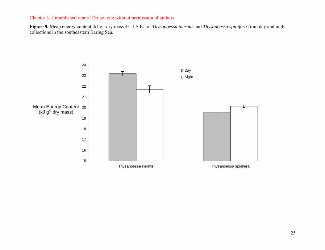
Chapter 3. Unpublished report: Do not cite without permission of authors.
Figure 9. Mean energy content [kJ g-1 dry mass +/- 1 S.E.] of Thysanoessa inermis and Thysanoessa spinifera from day and night collections in the southeastern Bering Sea.
15
16
17
18
19
20
21
22
23
24
Thysanoessa inermis Thysanoessa spinifera
Day
Night
Mean Energy Content (kJ g-1 dry mass)
25

Chapter 3. Unpublished report: Do not cite without permission of authors.
Figure 10. Comparison of 1) mean energy density [kJ m-3 +/- 1 S.E.] in the water column comprised by zooplankton and 2) zooplankton density [# m-3] in 0-100 m water depth in offshore and nearshore habitats.
1
8 6 4 2
0.1
111
0.00.00.00.0
Offshore Nearshor
Euphausia Copepo Chaetogna Hyperiid Mollus Larvace
Energy Density (kJ m-3)
20
7
6
5
4
3
2
1
304050
Euphausia Copepo Chaetogna Hyperiid Mollus Larvace
Zooplankton Density
3
26

Chapter 3. Unpublished report: Do not cite without permission of authors.
Appendix 1. Species composition from MN samples in the southeastern Bering Sea, June 10-20, 2005
Amphipoda Cyphocaris challengeri Hyperoche medusarum Parathemisto pacifica Primno macropa Bryozoa Cephalopoda Chaetognatha Sagitta sp. Cirripedia Cnidaria Copepoda
Calanoida
Acartia longiremis Calanus marshallae Calanus pacificus Candacia columbiae Centropages abdominalis Chiridus sp. Eucalanus bungii Euchaeta elongata Gaetanus intermedius Heterorhabdus spp. Metridia pacifica Neocalanus cristatus Neocalanus spp. Pleuromamma scutullata Aetidius spp.
Cyclopoida Oithona sp. Harpacticoida Ctenophora
Hydrozoa Siphonophora
Decapoda
Rhinolithodes wosnessenskii (rhinoceros crab) Paralithodes camtschaticus (red king crab) Telmessus chaeiragonus (helmet crab) Acantholithodes hispidus (spiny lithoid crab) Erimacrus isenbeckii (hair crab) Cryptolithodes sp.
Echinodermata Euphausiacea
Euphausia pacifica Thysanoessa inermis Thysanoessa longipes Thysanoessa spinifera Tessarabrachion oculatum
Isopoda Mollusca Gastropoda Clione limacina
Limacina helicina Pisces Polychaeta Tomopteris spp. Ostracoda Conchoecia sp. Tunicata Larvacea Oikopleura sp.
27

Chapter 4. Unpublished report: Do not cite without permission of authors.
Aerial remote sensing and ecological hot spots in the southeastern Bering Sea
Evelyn D. Brown1 and James H. Churnside21School of Fisheries and Ocean Science, University of Alaska Fairbanks, Fairbanks, AK 99775-7220
2NOAA, ETL, 325 Broadway R/E/ET2, Boulder, CO 80305
Abstract
Ephemeral ecological hot spots comprising thousands of seabirds, marine mammals predating
on immense swarms of euphausiids and schooling forage fish were tracked using aerial remote sensing
and visual counting methods. These hot spots were large enough to cause a surface effect visible from
space using Synthetic Aperature Radar (SAR). These foraging event hot spots may be difficult to
locate and track without using measurement techniques that can cover large areas in a short amount of
time. These events may be critical in the life history of apex predators, represent the exchange of
enormous amounts of trophic energy, and exert strong top-down control on ecologically and
economically important forage fish species such as herring or capelin. Over a ten-day period, 7900 km
of continental shelf, slope, and nearshore marine habitats were surveyed by aircraft in the southeastern
Bering Sea, an ecological productive area. Geolocated data collected included visual observations,
quantified subsurface features with airborne lidar (light detecting and ranging), SST via an infrared
radiometer, and SAR imagery overlapping the times and locations of the aerial surveys. The hot spots
occurred at the shelf slope, were approximately 5 nmi in diameter, and comprised humpback whales,
Dall porpoise, and thousands of sooty shearwaters, fulmar, and other pelagic seabirds. Underlying the
apex community was a concentration of patchy fish schools and euphausiid swarms ranging in size of
10s to 100s of meters in diameter, averaging 10 m thick, and ranging in the upper 30 m of the water
column. Using spatial correlation, fish school locations were significantly (p < 0.001) correlated with
apex predator counts and bathymetry but not SST. These hot spot events exhibited daily fluctuations in
magnitude and location. Documenting and tracking this spatial variation would be difficult with slow
moving ships. More studies are needed to determine what physical and biological factors govern their
appearances. It is possible grazing pressure on plankton and local weather patterns affect distribution
and movements of forage fish and euphausiids (also extremely abundant here) which in turn affects
distributions and movements of apex predators. To our knowledge, this is the first attempt to track and
describe such events in the Bering Sea using remote sensing.
1

Chapter 4. Unpublished report: Do not cite without permission of authors.
Introduction
While the importance of forage species to healthy ecosystem functioning is widely accepted,
targeted and comprehensive studies on many of those species are non-existent. In 1999, amendments to
Alaskan groundfish management plans created a new forage fish category to allow for specific
management actions intended to conserve and manage forage fish resources. However, without critical
life history, distribution and abundance information on these species, the effects of targeted
management actions will be poorly understood and possibly immeasurable with the current array of
assessment tools in place.
Despite the present information gaps, over the past 100 years a multitude of studies have
occurred in the Bering Sea region that include information on the listed forage taxa (squid, osmerids or
smelt, bathylagids or deepsea smelt, clupeids or herring, ammodytids or sand lance, and myctophids or
lanternfishes) and the diverse oceanographic environments that they occupy. All of these species are
considered pelagic but some have seasonal affinities to nearshore zones (< 50 m depths) while others
spend their entire lives in deepwater regions (> 250 m depths). Some species (e.g. squid) appear to
concentrate along the “green belt” (see Figure 1) The diverse life histories, distributions, and
population dynamics will likely dictate a similarly diverse array of survey designs and assessment tools
needed to for management or protective measures. Much of the information from these studies has
been summarized in books, workshop or symposium proceedings and some data is available on line or
obtainable from former investigators (Table 1).
From a preliminary overview of the literature, key species and their associated habitats can be
defined (Table 2). Habitat ranges are listed by domain or regions in the Bering Sea defined by
bathymetric contours (Figure 1): coastal domain (50 m or shallower), middle domain (between 50 and
100 m), outer domain (between 100 and 200 m) and oceanic domain or basin (over 200 m). Future
studies may reveal other key species that are important but poorly understood in terms of ecological
importance. For example, stomiidae (dragonfish) and notosudidae (waryfishes), although not on the
proposal request list of taxa, were listed as the third and fourth most abundant mesopelagic fish in the
western Bering Sea following myctophidae and bathylagidae (Sobolevsky et al. 1996). Other unlisted
fish, Pacific sandfish (Trichodon trichodon) and juvenile salmon (Onchorhynchus spp.) may be
important regionally based on abundance in the nearshore (Livingston 2002; Farley et al. 2000). In
addition, juvenile walleye pollock (Theragra chalcogramma), euphausiids (e.g. Thysanoessa spp.), and
gelatinous macrozooplankton (jellyfish) may need to be included in ecosystem modeling or assessment
2

Chapter 4. Unpublished report: Do not cite without permission of authors.
of targeted forage taxa because of the sheer abundance and ecological importance to other forage taxa
as well as the apex community (see Coyle and Pinchuk, Brodeur et al., Hunt et al., and Stabeno et al.
2002, Deep-Sea Research II 49). Some of the listed species (e.g. Pacific herring, capelin, and squid)
are better understood than others because they are abundant and are or were targeted in fisheries.
However, none of the species in the list (Table 2) have been the focus of ecosystem-based studies and
therefore trophic relationships and top-down or bottom-up forcing processes are poorly understood.
Given the gap in understanding of most aspects concerning forage species in the Bering Sea, a
pilot study with multiple investigators was initiated with the goal of assessing distribution, species
composition, and the ecological role of forage species within the nearshore, continental shelf, and
continental slope habitats as well as the technologies and techniques used to collect them. As part of
this ambitious study, our role was to assess the utility of aerial remote sensing in the study of forage
species. Our rationale was that many of the forage species are planktivorous, are therefore associated
with surface, plankton-rich waters, and are often accompanied by a host of surface-dwelling or
associated apex predators. These species are good candidates for remote sensing from the air.
The patchy and contiguous distribution of schooling fish, such as capelin (Mallotus villosus)
requires large numbers of sampling units or transects to achieve statistical validity of assessments if a
priori information is not available (Cram and Hampton, 1976; Fiedler, 1978; Barange and Hampton,
1997). Ship survey methods are slow and therefore costly, and generally sample narrow swaths of
water. When fish schools are near the surface, acoustic biomass estimates can be unrealistically low
(Vilhjálmsson, 1994). Ship and net avoidance can confound biological assessments of fish and
ecological research on the relationships between predators and their fish prey (Aglen and Misund,
1990; Olsen, 1990; Logerwell and Hargreaves, 1996).
Water penetrating instrumentation, such as LIght Detecting and Ranging (LIDAR), are being
used with increasing frequency from aircraft as the technology is developing. Blue-green light
propagates to depths up to 100 m (Squire and Krumboltz, 1981) and green lasers have been applied in
the form of lidar (light detection and ranging), where photon backscatter is collected from light
reflecting off biological targets in the water column. Although numerical algorithms for lidar detection
of fish were established more than 20 years ago (Murphree et al., 1974), modelling of signal-to-noise
ratio, estimation of fish abundance, and statistical treatment of lidar data is a continuing area of
research (Krekova et al., 1994; Mitra and Churnside, 1999; Lo et al., 2000). Target strength is a
function of green-light reflectivity and has been measured on frozen samples of several fish species
3

Chapter 4. Unpublished report: Do not cite without permission of authors.
(Churnside and McGillivary, 1991), and live sardines in a tank experiment (Churnside et al., 1997).
Airborne lidar has also been used to detect subsurface oceanic scattering layers (Hoge et al., 1986]). In
the early 1990s, the Fish Lidar Oceanic Experimental (FLOE) system was constructed from off-the-
shelf components, and improvements were made to signal-processing techniques used to discriminate
fish returns from small particles in the water (Churnside et al., 1998, 2001a). The FLOE system
penetrates depths up to 50 m, and has been used off the coast of California to survey anchovy and
sardine (Churnside et al., 1997; Hunter and Churnside, 1995; Lo et al., 2000), and has more recently
been used to measure plankton, squid, and marine mammals (Churnside et al., 2001a). The FLOE
system was first used in Alaska and used to document large schools of capelin and map variations in
plankton distribution in the Gulf of Alaska (Brown et al. 2002). Comparisons of LIDAR with acoustic
data have been very encouraging, and these methods can produce similar results (Churnside et al.,
2001b). Spain is developing a program for sardine assessment that incorporates LIDAR and Norway is
undertaking commercially available fish LIDAR instrumentation.
Methods
This study was conducted in the southeastern Bering Sea along the northern coasts of Unalaska,
Akutan and Akun Islands (Figure 2). Oceanographic descriptions of this location are covered in
Chapters 1 and 3 of this report. Aerial surveys were designed to bracket a coordinated ship survey (see
Chapters 1-3) extending and tripling the area transected by the vessel in order to provide a broadscale
view of the area and to address how well the ship regions represented distributions for near-surface
schools and surface predators. The ship surveyed two regions, one nearshore and one offshore covering
shelf and slope habitat. In addition, ship survey tracks were repeatedly measured (5 times during the
day and twice at night) in order to gain a better understanding of short term variation of biological
features observed. Aerial surveys were flown from June 8 through June 19, 2006.
Instrumentation mounted on the aircraft consisted of the LIDAR, and infrared radiometer used
to measure sea surface temperature, and an RGB high resolution camera. The LIDAR system was used
and is described in detail by Churnside et al. (2001). It is a non-scanning, radiometric LIDAR with
three major components: (1) the laser and beam-control optics, (2) the receiver optics and detector, and
(3) the data collection and display computer. The laser is linearly polarized and the beam diverged,
using a lens in front of the laser, to meet eye-safety standards established for marine mammals (Zorn et
al., 2000). During the day, a narrower divergence filter is used than at night, when it is three times
4

Chapter 4. Unpublished report: Do not cite without permission of authors.
wider. The narrow filter minimizes the amount of background light entering the receiver, but
effectively limits the penetration depth of laser light (Gordon, 1982). A polarizer in front of the
telescope selects the cross-polarized component of the reflected light, thus maximizing contrast
between fish and smaller light-scattering particles (Churnside et al., 1997; Lewis et al., 1999). The
telescope collects the light onto an interference filter to reject background light. As with the divergence
filter, a narrow interference filter is used by day and a wider one at night. An aperture at the focus of
the primary lens also limits background light by limiting the field of view of the telescope to match the
divergence of the transmitted laser beam. The resulting light is incident on a photomultiplier tube,
which converts the light into an electrical current. For the night-time receiver, the active area of the
photomultiplier tube is the field-stop aperture. By day, a separate aperture is used, and the light is
transferred to the photomultiplier tube by a second lens. The combination of divergence lens size,
field-of-view setting, interference filter width, and altitude flown in 2000 determined the spot diameter
or sampling swath at 5 m by day and 15 m by night. The photomultiplier tube output is passed through
a logarithmic amplifier to increase the dynamic range of the signal. A 50-Ω load resistor converts the
current in a voltage, which can be digitized in the computer.
LIDAR signal was processed according to the protocols established earlier (Churnside et al.
1997) with the main goal of removing the background signal attributable to water. Signal above
background was sorted by applying thresholds to sort out the plankton scattering contribution versus
fish with a multi-scale expansion to aid in target identification. The multi-scale expansion was based
on the Multiresolution Median Transform (MMT) (Starck et al, 1998). Preliminary results produced a
correlation of R2 = 0.97 between LIDAR return strength, integrated over depth, and the catch of
sardines when a median filter of 150 m along the flight track was applied. When the filter length was
doubled to 300 m using the same data, the correlation was reduced to R2 = 0.35. This suggests that the
horizontal scale of the LIDAR return can be an important clue to target identification.
Processed signal was sorted into two main categories, weak scattering layers representing
plankton and strong discriminate signal aggregations representing fish schools. In addition, the
penetration depth (point at which laser light attenuates) is recorded from data processing is a function
of water clarity and phytoplankton content (Brown et al. 2002). Within the context of this report, we
describe only the fish signal in relation to the apex predator community.
5

Chapter 4. Unpublished report: Do not cite without permission of authors.
Visual counts were obtained on seabird and mammals following protocols established during
previous similar surveys (Brown et al. 2002). Counts were geocoded by measuring the time of the
observation and linking that time to the geocoded flight track recorded by the instrument GPS units.
SAR data was obtained and processed from imagery and software available at the Alaska SAR
Facility at the University of Alaska. Images were selected based on temporal overlap with the survey
period. SAR images basically show changes in sea surface roughness and internal waves. Bright spots
in the images are produced by large metal objects (e.g. ships) and other large surface formations such
as the hot spot observed. The resolution of the images obtained was 12.5 m (pixel resolution) at the
surface.
In order to test the relationship between physical variables and fish distribution and between
fish distribution and apex predators, spatial linear models were derived in the form of generalized least
squares regression. The model form and process is described by Kaluzny et al. 1998 and the statistical
program SPlus was used to analyze the data.
Results
In total, we flew the LIDAR just under 7900 km (Figure 2). Of these, about 11% were within
the offshore box (shelf and slope habitat) surveyed by the vessel and 16% within the nearshore box.
Most of the fish schools detected by the LIDAR were outside of these regions. Of 830 schools, only
20 were within the offshore box and 30 within the nearshore box. The resulting density of schools was
0.023 ± 0.005 schools / km within the offshore box, 0.024 ± 0.004 schools / km within the nearshore
box, and 0.105 ± 0.004 schools / km for all flights. The average school length was 87.5 m. Average
depth of the schools was 6.2, 5.4, and 5.2 m for the offshore, nearshore, and all schools, respectively.
The probability density function of depth shows that the nearshore schools have a secondary peak in
the 12-18 m depth bin (Figure 3).
Describing observations sequentially within the ship survey regions, in the offshore area:
June 8: We covered the entire box and detected no schools within.
June 9: We covered the entire box and detected 2 schools in the SE corner at about 2300 UTC. There
was also a strong layer in about the top 2 m. This layer was not always at the surface, and
seemed to go deeper to avoid surface predation.
June 11: We covered the entire box and detected no schools within.
6
Chapter 4. Unpublished report: Do not cite without permission of authors.
June 12: We covered the entire box and detected no schools. Later, we covered the north and east
parts of the box, and saw several schools along the north edge. The first coverage of the
northern part of the box was between about 10:20 UTC and 11:20 UTC. The schools were
observed a little less than 2 hours later at about 13:15 UTC.
June 14: We covered the entire box, although not as densely as on previous days. Two schools were
detected in the SE corner of the box at about 19:49 UTC.
June 17: We only covered the southern part of the box, but detected more schools than previously.
The time was between about 22:45 and 22:50 UTC. More schools were also detected just south
of the box.
In the nearshore area:
June 8: We covered 3 lines on the western side of the box and detected 1 school near the southern
edge at 21:23 UTC.
June 9: We covered the western part of the box and detected 2 schools near the NW corner at about
21:20 and 1 near the center in the southern part at about 22:00.
June 13: We covered most of the box with 2 schools detected in the northern part at 1:25 and 1:52
UTC. More schools were detected just to the north of the box. At about the same time, a
number of schools were detected very close to shore off the point the north of Lost Harbor.
June 17: We covered the eastern part of the box, and detected several schools near the southern edge
in shallow water.
June 18: We covered the entire box and detected the most schools of any flight over this region.
Three were in the same shallow-water region as on the 17th, and the rest were spread through
the center of the bay.
June 19. Three widely spaced schools were detected in another fairly complete coverage of the box.
Generally, the school density was too sparse to interpolate.
Given the results of the observations within the ship survey area, we decided to evaluate the
region as a whole within the confines of the aerial flight paths and were able to describe the formation
of the hot spots. The hot spots occurred at the shelf slope, were approximately 5 nmi in diameter, and
comprised humpback whales, Dall porpoise, and thousands of sooty shearwaters, fulmar, and other
pelagic seabirds. Underlying the apex community was a concentration of patchy fish schools and
euphausiid swarms ranging in size of 10s to 100s of meters in diameter, averaging 10 m thick, and
ranging in the upper 30 m of the water column. On the first survey day, June 8, we observed a
7

Chapter 4. Unpublished report: Do not cite without permission of authors.
concentration of seabirds north of Akutan Island (Figure 4). By July 9th, fish schools and whales began
to accumulate in the same area (Figure 5). On June 11th, large numbers of seabirds began to
accumulate in the region resulting in a feature that could be discerned from space using SAR imagery
(Figures 6 and 7). One can only appreciate the size of this feature by observation from the surface
(Figure 8). By June 13th, the feature was enormous (Figure 9). On June 16, fish schools dissipated at
the surface along with the seabirds and marine mammals (Figure 10). The original hot spot reformed
on June 17th along with a secondary one between Unalaska and Akutan Islands (Figure 11). By June
18th only the original hot spot remained (Figure 12). On the last day of survey (June 19), the main hot
spot appeared to have shifted westward along the shelf moving in the same direction as the residual
current in the area (see Chapter 3 for description of currents). The seabirds as well as the schools were
observed with the LIDAR in addition to the visual counts (Figure 14). The association of the two
features was clear from those results.
Spatial regression analysis indicated a significant ((p < 0.001) correlation between seabird and
fish school distribution as well as between fish school and bathymetry (bottom depth) with surface fish
schools concentrated on the shelf. There was not a significant correlation between fish schools and
SST detected by the infrared radiometer.
Conclusions
• Fish school density was lower in the originally designated study area than in the surrounding area.
Therefore, pre-selecting transects or survey regions, as opposed to adaptively selecting and/or
tracking features, is not a good way to assess surface forage species and ephemeral bouts of
foraging and energy exchange
• Using aircraft allowed coverage over a large region and repeat measurements, we were able to map
and measure temporal variability within the hot spots.
• Given the enormous numbers of apex predators and fish schools surveyed within the hot spots, they
probably represent a significant portion of trophic energy exchange occurring within the region
among these species.
• Fish schools were probably aggregating on the shelf due to the high concentrations of copepods
and euphausiids there (see Chapter 3).
• The large numbers of seabirds changed the surface roughness of the ocean to a degree that the hot
spot was visible with SAR imagery.
8

Chapter 4. Unpublished report: Do not cite without permission of authors.
• Aerial remote sensing should be developed to assess surface schooling or aggregating features (e.g.
capelin, herring, sand lance, euphausiids, and plankton) where features are patchy and where they
exhibit a large degree of temporal variability, such as we observed.
• An adaptive survey design, using a moving grid, to track and sample these features with directed
ship sampling would result in an improved assessment of the surface forage species and foraging
events.
Acknowledgements
We would like to thank Commander Northwest and our attentive pilot Marco for providing a
mechanically reliable aircraft and for protecting our safety. We would like to thank Mike Sigler for
organizing and overseeing this project. We would like to thank James Wilson for assistance with
equipment engineering, installation, and operation. We would like to thank Christopher Kenaley for
the use of his photograph. Funding for this research was supported with a grant from the North Pacific
Research Board, project # F0401.
Literature Cited
Aglen, A. and Misund, O. A. 1990. Swimming behaviour of fish schools in the North Sea during
acoustic surveying and pelagic sampling trawling. ICES CM 1990/B: 38.
Barange, M., and Hampton, I. 1997. Spatial structure of co-occurring anchovy and sardine populations
from acoustic data: implications for survey design. Fisheries Oceanography, 6: 94–108.
Brodeur, R.D., M.T. Wilson, L. Ciannelli, M. Doyle, and J.M. Napp. 2002. Interannual and regional
variability in distribution and ecology of juvenile pollock and their prey in frontal structures of the
Bering Sea. Deep-Sea Res. II. 49: 6051-6067.
Brown, E.D., Churnside, J.H., Collins, R.L., Veenstra, T., Wilson, J.J., and Abnett, K. 2002. Remote
sensing of capelin and other biological features in the North Pacific using lidar and video
technology. ICES Journal of Marine Science, 59: 1120-30.
9

Chapter 4. Unpublished report: Do not cite without permission of authors.
Churnside, J. H., and McGillivary, P. A. 1991. Optical properties of several Pacific fishes. Applied
Optics, 30: 2925–2927.
Churnside, J.H., Wilson, J.J., and Tatarskii, V.V. 1997. Lidar profiles of fish schools. Applied Optics,
36: 6011–6020.
Churnside, J.H., Wilson, J.J., and Tatarskii, V.V. 2001. An airborne lidar for fisheries applications.
Optical Engineering, 40: 406–414.
Churnside, J. H., Sawada, K., and Okumura, T. 2001b. A comparison of airborne lidar and echo
sounder performance in fisheries. Journal of the Marine Acoustical Society of Japan, 28: 49–61.
Churnside, J.H., D.A. Demer, and B. Mahmoudi. 2003. A comparison of lidar and echosounder
measurements of fish schools in the Gulf of Mexico. ICES Journal of Marine Science 60: 147-154.
Coyle, K.O. and A.I. Pinchuk. 2002. The abundance and distribution of euphausiids and zero-age
pollock on the inner shelf of the southeast Bering Sea near the Inner Front in 1997-1999. Deep-Sea
Research II 49: 6009-6030.
Craig, J.F., M. J. Kenley and J.F. Talling. 1978. Comparative estimations of the energy content of fish
tissue from bomb calorimetry, wet oxidation and proximate analysis. Freshwater Biology 8:585-
590.
Craig, P. 1987. Forage fishes in the shallow waters of the North Aleutian shelf. Pages 49-54 in Forage
Fishes of the Southeastern Bering Sea Conference Proceedings, U.S. Dept. of the Interior, Minerals
Management Service Report July 1987.
Cram, D. L., and Hampton, I. 1976. A proposed aerial/acoustic strategy for pelagic fish stock
assessment. Journal du Conseil International pour L’Exploration de la Mer, 37: 91–97.
Farley, E.V., Jr., R.E. Haight, C.M. Guthrie, and J.E. Pohl. 2000. Eastern Bering Sea (Bristol Bay)
coastal research on juvenile salmon, August 2000. (NPAFC Doc. 499) Auke Bay Laboratory,
10

Chapter 4. Unpublished report: Do not cite without permission of authors.
Alaska Fisheries Science Center, NMFS, NOAA, 11305 Glacier Highway, Juneau, AK 99801-8626.
18 p.
Fiedler, P. C. 1978. The precision of simulated transect surveys of northern anchovy, Engraulis
mordax, school groups. Fishery Bulletin U.S., 76: 679–685
Gordon, H. R. 1982. Interpretation of airborne oceanic lidar: effects of multiple scattering. Applied
Optics, 21: 2996–3001.
Hoge, F. E., Berry, R. E., and Swift, R. N. 1986. Active–passive airborne ocean color measurement. 1.
Instrumentation. Applied Optics, 25: 39–47.
Houghton, J.P. 1987. Forage fish use of inshore habitats north of the Alaska Peninsula. Pages 39-48 in
Forage Fishes of the Southeastern Bering Sea Conference Proceedings, U.S. Dept. of the Interior,
Minerals Management Service Report July 1987.
Hunt Jr., G.L., C. Baduini, J. Jahncke. 2002. Diets of short-tailed shearwaters in the southeastern
Bering Sea. Deep-Sea Research II 49: 6147-6156.
Hunter, J. R., and Churnside, J. M. 1995. Airborne fishery assessment technology: a NOAA workshop
report. NOAA Southwest Fisheries Science Center Administrative Report, La Jolla, California, LJ–
95–02. 71 pp.
Kaluzny, S.R., S.C. Vega, T.P. Cardoso, and A.A. Shelly. 1997. S+ spatial stats. Springer, New York.
Lewis, G. D., Jordan, D. L., and Roberts, P. J. 1999. Backscattering target detection in a turbid
medium by polarization discrimination. Applied Optics, 38: 3937–3944.
Livingston, P. (ed.) 2002. Ecosystem considerations for 2003. Available
http://www.fakr.noaa.gov/npfmc/safes/safe.htm.
11
Chapter 4. Unpublished report: Do not cite without permission of authors.
Livingston, P., K. Aydin, J. Boldt, S. Gaichas, J. Ianelli, J. Jurado-Molina, and I. Ortiz. 2003.
Ecosystem Assessment of the Bering Sea/Aleutian Islands and Gulf of Alaska Management
Regions. Available Alaska Fisheries Science Center.
Lo, N. C. H., Hunter, J. R., and Churnside, J. H.. 2000. Modeling statistical performance of an airborne
lidar survey system for anchovy. Fishery Bulletin U.S., 98: 264–282.
Logerwell, E. A., and Hargreaves, N. B. 1996. The distribution of sea birds relative to their fish prey
off Vancouver Island: opposing results at large and small spatial scales. Fisheries Oceanography, 5:
163–175.
Mecklenberg, C. W., T. A. Mecklenburg, and L. K. Thorsteinson. 2002. Fishes of Alaska. American
Fisheries Society. Bethesda, Maryland. 1037 p.
Mitra, K., and Churnside, J. H. 1999. Transient radiative transfer equation applied to oceanographic
lidar, Applied Optics, 38: 889–895.
Murphree, D. L., Taylor, C. D., and McClendon, R. W. 1974. Mathematical modeling for the detection
of fish by an airborne laser. Journal of the American Institute of Aeronautics and Astronautics,
12: 1686–1692.
Naumenko, E. A. 1996. Distribution, biological condition and abundance of capelin (Mallotus
villosus) in the Bering Sea. In: Ecology of the Bering Sea: A review of Russian Literature, p.
237-256. Ed. O. A. Mathisen and K. O. Coyle, Ecology of the Bering Sea, Univ. Alaska Sea
Grant College Program. Rpt. 97/01. 306 p.
Olsen, K. 1990. Fish behaviour and acoustic sampling. Rapports et Procès-Verbaux des Réunions du
Conseil International pour l' Exploration de la Mer, 189: 147–158.
Orlov, A.M. 1997. Mesopelagic fishes as prey of Atka mackerel (Pleurogrammus monopterygius,
Hexagrammidae, Scorpaeniformes) off the northern Kuril Islands. Pages 323-335 in Forage
12

Chapter 4. Unpublished report: Do not cite without permission of authors.
Fishes in Marine Ecosystems, University of Alaska Sea Grant College Program Report No. 97-
01.
Pahlke, K. A. 1985. Preliminary study of capelin (Mallotus villosus) in Alaskan waters. ADFG Info.
Lflt. 250. 64 p.
Robards, M. and M. Schroeder. 2000. Assessment of nearshore fish around Akutan Harbor using
beach seines during March and July 2000. USGS Biological Resources Division, Alaska,
Biological Sciences Center, 1011 E. Tudor Road, Anchorage, AK 99503.
Sinclair, E.H. and P.J. Stabeno. 2002. Mesopelagic nekton and associated physics in the southeastern
Bering Sea. Deep-Sea Research II 49: 6127-6146.
Sobolevsky, Y.I., T.G. Sokolovaskaya, A.A. Balanov, and I.A. Senchenko. 1996. Distribution and
trophic relationship of abundant mesopelagic fishes of the Bering Sea. Pages 159-168 in
Mathisen, O.A. and K.O. Coyle, editors, Ecology of the Bering Sea, University of Alaska Sea
Grant College Program, Report No. 96-01.
Squire, J.L. Jr. and H. Krumboltz, “Profiling pelagic fish schools using airborne optical lasers and
other remote sensing techniques,” Mar. Tech. Soc. J. 15, 27-31 (1981).
Starck, J-L, F. Murtagh, and A. Biuaoui (1998), Image Processing and Data Analysis (Cambridge
University Press, Cambridge).
Stabeno, P.J. and G.L. Hunt, Jr. 2002. Overview of the Inner Front and southeast Bering Sea carrying
capacity programs. Deep-Sea Research II 49: 6157-6168.
Tsarin, S.A. 1997. Myctophids of the sound scattering layer and their place in pelagic food webs.
Pages 271-275 in Forage Fishes in Marine Ecosystems. University of Alaska Sea Grant College
Program Report No. 97-01.
13

Chapter 4. Unpublished report: Do not cite without permission of authors.
Viihjálmsson, H. 1994. The Icelandic capelin stock. Rit Fiskideildar, 13: 281 pp.
Watanabe, H., M. Masatoshi, K. Kawaguchi, K. Ishimaru, and A. Ohno. 1999. Diel vertical migration
of myctophid fishes (Family Myctophidae) in the transitional waters of the western North
Pacific. Fisheries Oceanography 8(2): 115-127.
Wespestad, V. G. 1991. Pacific herring population dynamics, early life history, and recruitment
variation relative to eastern Bering Sea oceanographic factors. Doctoral dissertation, University
of Washington, Seattle.
Wilson, J.R. and A.H. Gorham. 1982. Alaska underutilized species Volume 1: Squid. Alaska Sea Grant
Report 82-01.
Zorn, H.M., Churnside, J.H., and Oliver, C.W. 2000. Laser safety thresholds for cetaceans and
pinnipeds. Marine Mammal Science, 16: 186–200.
14

Chapter 4. Unpublished report: Do not cite without permission of authors.
Table 1. A partial list of research programs and published proceedings or books containing information on forage taxa in the Bering Sea.
Type Mo/Yr Resource or Citation Government Report May 1978 Resources of Non-Salmonid Pelagic Fishes of the Gulf of Alaska and Eastern
Bering Sea. Macy et al. NOAA NMFS Report (no report no.) Sea Grant Report 1982 Alaska Underutilized Species Volume 1: Squid. Wilson and Gorham, July 1982.
Alaska Sea Grant Report 82-1. NMFS Trawl Survey Results
1982-present
Forage fish bycatch in stock assessment trawls surveys; Livingston 2003 and other report from NMFS AFSC, Kodiak and Seattle labs
Japanese Research Cruises and Commercial Fishing Catches
1970s to present
Data from the Japanese Fisheries Agency and its research vessels, i.e. the Oshoro Maru, have recently been made available. This data set includes net samples of gillnets, trawls, longlines and jigging equipment.
OCSEAP & PROBES mid-1970s-late 1980s
resource assessments from the Outer Continental Shelf Environmental Assessment Program and research results from the Processes and Resources of the Bering Sea study
Workshop Proceedings Oct. 1983 Proceedings of the workshop on biological interactions among marine mammals
and commercial fisheries in the southeastern Bering Sea. Alaska Sea Grant Report 84-1. UAF. April 1984
Conference Proceedings July 1987 Forage Fishes of the Southeastern Bering Sea, USDI MMS, Alaska OCS Region Workshop Summary March
1991 Is It Food? Addressing Marine Mammal and Seabird Declines. Alaska Sea Grant Report 93-01. UAF, 1993.
Bering Sea FOCI 1991-1997
A coordinated series of federally funded studies with NMFS AFSC as the lead agency and conducted by researchers from the NMFS AFSC, NOAA PMEL, UAF and other universities.
Book 1996 Ecology of the Bering Sea: A Review of Russian Literature. Mathisen and Coyle. University of Alaska Sea Grant College Program Report No. 96-01.
Symposium Proceedings Nov. 1996 Forage Fishes in Marine Ecosystems. Proceedings of the International Symposium on the Role of Forage Fishes in Marine Ecosystems. University of Alaska Sea Grant College Program Report No. 97-01.
SMMOCI 1995-1997
A coordinated series of federally funded studies with NMFS NMML as the lead agency and conducted by researchers from NMFS AFSC & NMML, NOAA PMEL, University of Alaska Fairbanks and others.
SEBSCC & IFP 1995-2000
A series of coordinated studies funded by the NSF Office of Polar Programs and conducted by researchers from UAF, NOAA PMEL, NNFS NMML and NMFS AFSC and other academic organizations. The dedicated volume below shows results from these studies.
Dedicated Journal Volume
2002 Ecology of the Southeastern Bering Sea. Deep-Sea Research Part II, Volume 49, No. 26. Milliman, editor.
BASIS & SEBSOCC 1999-present
A coordinated series of studies with NMFS as the lead agency and with international participants with a goal of understanding the marine phase of Pacific salmon.
15

Chapter 4. Unpublished report: Do not cite without permission of authors.
Table 2. A list of key forage fish species and the main habitat ranges observed within the Bering Sea.
Family/Species Common Name
Habitat Reference
Gonatidae squid
outer domain, shelf break; exhibit extreme vertical migrations
Wilson and Gorham 1982; Sinclar and Stabeno 2002
Berryteuthis magister Gonatopsis borealis Onychoteuthis banskii borealis
Osmeridae smelt
Mallotus villosus capelin seasonal migrations through coastal, middle and outer domains; surface to 200 m depths
Paulke 1985; Craig 1987; Houghton 1987; Naumenko 1996; Livingston 2002; NMFS AFSC trawl data
Hypomesus olidus pond or silver smelt
some are anadromous; mainly occupy river estuaries and coastal domain
Houghton 1987; Naumenko 1996;
Hypomesus pretiosus surf smelt limited range in coastal domain around western end of Alaska Peninsula
Houghton 1987; Robards and Schroeder 2000; Mecklenburg et al. 2002
Osmerus mordax rainbow or Arctic smelt
anadromous with seasonal migrations through coastal, middle and outer domains; surface to 150 m
Craig 1987; Naumenko 1996; Mecklenburg et al. 2002
Thaleichthys pacificus eulachon anadromous with seasonal migrations through coastal, middle and outer domains apparently restricted to eastern shelf; surface to 300m
Houghton 1987; Mecklenburg et al. 2002; Livingston 2002; NMFS AFSC trawl data
Bathylagidae deepsea smelt
Leuroglossus schmidti northern smooth-tongue
in deepwater from the outer domain and shelf break throughout basin; extreme vertical migrations between surface and 1800 m
Orlov 1997; Sinclair and Stabeno 2002; Mecklenburg et al. 2003
Bathylagus pacificus slender blacksmelt
in deepwater from the shelf break and over the basin; no vertical migration; found in depths of 150 to 7700 m
Sinclair and Stabeno 2002; Mecklenburg et al. 2003
Bathylagus ochotensis eared blacksmelt
in deepwater from the shelf break and over the basin; extreme vertical migration between the surface and 6,100 m
Sinclair and Stabeno 2002; Mecklenburg et al. 2003
Pseudobathylagus milleri stout blacksmelt
in deepwater from the shelf break and over the basin; extreme vertical migration between the 60 and 6,000 m
Sinclair and Stabeno 2002; Mecklenburg et al. 2003
Clupeidae herring
Clupea pallasi Pacific herring seasonal migrations through coastal, middle, and outer domains; vertically migrate from surface to 100 m
Wespestad 1991 and many others (best known species in list)
Ammodytidae sand lance
Ammodytes hexapterus Pacific sand lance
seasonal migrations through coastal and middle domains; surface to 100 m depths; bury themselves in sand when not schooling
Craig 1987; Farley et al. 2000; Robards and Schroeder 2000; Livingston 2002; Mecklenburg et al. 2003
Myctophidae lanternfish Tsarin 1997
Stenobrachius leucopsarus northern lampfish
in deepwater over the basin; extreme vertical migrations between 30 m and 1000 m
Watanabe et al. 1999; Sinclair and Stabeno 2002; Mecklenburg et al. 2003
Stenobrachius nannochir garnet lampfish
in deepwater over the basin; does not vertically migrate; found between 500 m and 1000 m
Watanabe et al. 1999; Sinclair and Stabeno 2002; Mecklenburg et al. 2003
Lampanyctus jordoni brokenline lanternfish
in deepwater over the basin; extreme vertical migrations between 200 m and 1400 m
Watanabe et al. 1999; Sinclair and Stabeno 2002; Mecklenburg et al. 2003
Nannobrachium regale (also as Lampanyctus regalis)
pinpoint lanternfish
in deepwater over the outer domain through the basin; extreme vertical migrations between the surface & 1500m
Watanabe et al. 1999; Sinclair and Stabeno 2002; Mecklenburg et al. 2003
Diaphus theta California headlight-fish
S. Bering Sea only along the shelf break from the Alaska Peninsula through the Aleutian Chain; extreme vertical migrations between the surface and 800 m
Watanabe et al. 1999; Sinclair and Stabeno 2002; Mecklenburg et al. 2003
16

Chapter 4. Unpublished report: Do not cite without permission of authors.
Figure 1. Domains and habitats of the eastern Bering Sea: 1a and 1b) SE and NW outer shelf, 2a and
2b) SE and NW middle shelf, 3) Pribilof Islands, 4) Unimak Island, 5) shelf break The “green belt” is
the area encompassed by the white oval http://www.pmel.noaa.gov/sebscc/concept). The study area
for this project is outlined by the yellow rectangle that encompasses the “horseshoe”, a fold in the
bathemetry that allowed study of multiple habitats (slope, shelf, and nearshore) within a relatively
small area.
17

Chapter 4. Unpublished report: Do not cite without permission of authors.
Figure 2. The cumulative aerial survey flight path (gray lines) or sampled transects from June 8 to June 19, 2006.
18

Chapter 4. Unpublished report: Do not cite without permission of authors.
Figure 3. The probability density function of depth of schools detected by LIDAR.
0
0.1
0.2
0.3
0.4
0.5
0.6
0.7
0.8
0 5 10 15 20 25 30 35 40
depth (m)
p(depth) PoffPnearPtot
19

Chapter 4. Unpublished report: Do not cite without permission of authors.
Figure 4. The first identification of the hot spot on June 8 mainly indicating the presence of large numbers of seabirds.
Fig. 2Hot Spot First Identified by Sea Birds
Fig. 2Hot Spot First Identified by Sea Birds
20

Chapter 4. Unpublished report: Do not cite without permission of authors.
Figure 5. Evolution of the hot spot continued June 9 with the appearance of baleen whales and fish schools.
Whales and Fish Schools NextWhales and Fish Schools Next
21

Chapter 4. Unpublished report: Do not cite without permission of authors.
Figure 6. The build up of seabird numbers continues on June 11.
Build-Up ContinuesBuild-Up Continues
22

Chapter 4. Unpublished report: Do not cite without permission of authors.
Figure 7. SAR image where the large numbers of seabirds and marine mammals create a surface disturbance that can be observed from space.
23

Chapter 4. Unpublished report: Do not cite without permission of authors.
Figure 8. Photograph of the hot spot with the large concentrations of seabirds and marine mammals. Photo courtesy Christopher Kenaley.
24

Chapter 4. Unpublished report: Do not cite without permission of authors.
Figure 9. By June 13, the hot spot feature is immense.
25

Chapter 4. Unpublished report: Do not cite without permission of authors.
Figure 10. On June 16th, fish schools were no longer observed and the seabirds and marine mammals disapated.
Fig. 3 Hot Spot Disappears Out of Survey Area
26

Chapter 4. Unpublished report: Do not cite without permission of authors.
Figure 11. On June 17th, fish schools reappear and reform the hot spot as well as a secondary hot spot between Unalaska and Akutan Islands.
Two Hot Spots Appear
27

Chapter 4. Unpublished report: Do not cite without permission of authors.
Figure 12. By June 18th, the original hot spot remains and the secondary one disappeared.
Second Hot Spot Disappears, Original One Remains
28

Chapter 4. Unpublished report: Do not cite without permission of authors.
Figure 13. On June 19th, the hot spot drifted to the west in approximately the same direction as the residual ocean current.
Main Hot Spot Appears to Shift to the East (w/residual current)
29

Chapter 4. Unpublished report: Do not cite without permission of authors.
Figure 14. An example of a LIDAR echogram shows a large school at a depth of 30 – 40 m and a large number of birds at the surface.
30

1
Mesozooplankton distributions in the southeastern Bering Sea estimated using a Multinet sampler and an evaluation of semi-automated processing with ZooImage software
Mark C. Benfield1, Nicola Hillgruber2, Marianne Alford3, Sara Arndt4, Jeffrey Bacon3,
and Sean F. Keenan1,5
1Department of Oceanography and Coastal Sciences, Louisiana State University, Baton Rouge, LA 70803
2School of Fisheries and Ocean Science, University of Alaska Fairbanks, Juneau, AK 99801 3 College of Agriculture, Louisiana State University, Baton Rouge, LA 70803
4College of Basic Sciences, Louisiana State University, Baton Rouge, LA 70803 5Present Address: Fish and Wildlife Research Institute, Florida Fish and Wildlife Conservation Commission,
St. Petersburg, Florida 33701
Abstract
A series of vertically stratified mesozooplankton samples collected in the Bering Sea
north of Akutan Island were processed to estimate the vertical zonation of dominant taxa in the
upper 40m of the water column. Traditional manual processing using a microscope was
compared with semi-automated processing using a flatbed scanner and ZooImage software. The
latter approach used digitized images of plankton to generate abundance estimates. Results from
this comparison suggest that it can produce abundance estimates comparable with those
produced by manual counting. Vertical zonation patterns obtained by manual processing
suggested considerable differences in structure within the near-surface waters from samples
collected over a 2 day period. These data will be used to evaluate changes in lidar backscatter
from nearby areas.
Introduction
Collection of zooplankton samples is generally accomplished using various types of nets,
pumps and traps (Wiebe and Benfield, 2003). Such devices filter the contents of large volumes
of water producing samples that may contain thousands to hundreds of thousands of individuals.
Such samples contain a wealth of potential information that can be related to distributions of
higher trophic levels, physical and chemical hydrography, and signals from remote sensing
systems such as acoustics and lidar. Moreover, zooplankton time-series can provide valuable
data on ecosystem responses to climate change and regime-shifts (Hays et al. 2005). Before this
information can be obtained and analyzed, the samples must be processed. Processing normally
consists of subdividing the sample into a representative aliquot, which is then sorted, identified,
measured and enumerated. Sample processing requires a patient and well-trained expert capable
2
of working with a microscope for extended periods. Skill in recognizing taxonomic identification
features is essential if the organisms are to be correctly assigned to taxonomic categories. Sample
processing is the bottleneck in studies of zooplankton ecology and delays associated with
processing generally limit the rate at which information about the sample can be extracted.
There have been a number of attempts to reduce the amount of time required to process
zooplankton samples. Ortner et al. (1979) developed a silhouette photographic technique that
created a direct contact sheet image of the contents of a sample aliquot by pouring the sample on
a photographic emulsion, exposing it to light, and developing the image. This had the advantage
of providing a permanent record of the sample contents, which could be counted, measured, and
identified by viewing the silhouette image under a microscope. While the level of taxonomic
detail present in the silhouette was lower than in the preserved sample, it provided sufficient
information to identify to species for organisms where distinctive morphological features were
present, and to broader taxonomic levels, such as calanoid copepods, euphausiids, chaetognaths,
in most cases. Moreover, the silhouettes could be quantitatively subsampled by overlaying a grid
of cells and randomly selecting some cells for analysis. This approach was combined with a an
early micro-computer-based measurement and recording system that employed acoustic
localization to determine the position of a cursor on the silhouette (Peter Wiebe, Woods Hole
Oceanographic Institution, Pers. Comm.). In this way samples could be analyzed for abundance,
size and taxonomic composition in a reproducible and shorter time period than traditional
microscope-based analyses.
With the advent of digital scanners, silhouette images could be digitized at high-
resolution and analyzed using software packages that subsample the image, and permit the user
to identify and measure the contents of the digital image. Abundance can be determined from
counts and a knowledge of the area subsampled, sample aliquot, and the original sample volume.
The Matlab-based Digitizer software developed by the Woods Hole Oceanographic Institution
(http://globec.whoi.edu/software/digi_prog/WHOI_Silhouette_DIGITIZER.htm) is an example
of such a system.
Direct scanning of samples suspended in liquid was problematic with the early scanners
because vibrations induced by the stepper motor that moved the scanning head, blurred the
digitized image. New scanners are capable of digitizing images without perceptible vibration
making direct digitization of the contents of plankton samples feasible. Moreover, specialized

3
waterproofed scanners such as the ZOOSCAN (Gorsky and Grosjean, 2003; Grosjean et al.
2004) have been designed to facilitate rapid scanning of plankton samples.
Production of a 2D image of the contents of a plankton sample or aliquot is but one step
in reducing the time required to process a sample. Some or all of the contents of the image must
still be counted, identified, and measured. This step remains an obstacle to rapid processing of
zooplankton samples. Recent advances in machine vision and pattern recognition have lead to
parallel advances in computerized analysis of plankton images. The ZOOSCAN system has
specialized software for locating, extracting, measuring and counting particles within an image.
Such regions of interest (ROIs) may then be used for visual classification by a human, or
computerized classification by a machine using some feature-based classifier (e.g. Culverhouse
et al. 1996; 2003; Blaschko et al. 2005).
ZooImage is public-domain software developed for semi-automated or fully-automated
processing of digitized zooplankton samples. Semi-automated processing consists of ROI
extraction and measurement by ZooImage followed by sorting into taxonomic groups by a
human. Fully-automated processing consists of the former steps to produce a taxonomically-
verified set of training images, which are then used to classify unknown ROIs into taxonomic
categories by ZooImage. In this paper we present the results from studies that compared
traditional plankton sample processing with semi-automated processing by ZooImage.
Methods
Study Area
This study was undertaken in the southeastern Bering Sea along the north coast of the
Aleutian Islands (Fig. 1) in waters NE of Dutch Harbor. Four zooplankton sampling stations
were selected for use in this analysis. These stations corresponded to dates and times where an
airborne lidar system was operated. (see Hillgruber et al. 2006, Table 1 for details of zooplankton
sampling station characteristics).
Zooplankton Sampling
An opening/closing net system (Hydrobios MultiNet) equipped with five 335 µm mesh
nets was deployed from the side of the F/V Great Pacific. Each cast was designed to collect
samples from different parts of the water-column along a double-oblique trajectory (Fig. 2). The
net was deployed with all nets closed and net 1 was opened near the bottom of the downward

4
portion of the trajectory with subsequent nets opened electronically along the ascending portion
of the tow (Fig. 2). Upon recovery the samples were washed out of the net with seawater,
concentrated by sieving, and preserved in 5% formalin.
Manual Zooplankton Processing
Manual processing refers to sample processing performed by a human observer. Our
observers were undergraduate student employees in our laboratory who all had been trained in
zooplankton sorting and processing for at least one year. All samples were initially examined and
sorted under a dissecting microscope for fish, fish eggs, and large pteropods, which were
separated and retained. Samples were then split into two equal aliquots using a Folsom plankton
splitter. One split from each sample was sent to the University of Alaska Fairbanks, Juneau
Center for archiving and the remaining splits were used in this study. All sample processing
performed by humans was conducted using plankton sorting trays under a dissection microscope
with counters to tally the abundance of taxa in each category. Since the data from these samples
was required for a related study examining the signals produced by plankton in response to lidar
illumination, our requirement for taxonomic resolution was coarse. The taxonomic categories we
used were: copepods, thecosomate pteropods, hyperiid amphipods, chaetognaths, euphausiids,
larvaceans, crab zoea, fish, and other zooplankton.
ZooImage
ZooImage is a software package written in R that employs the Java-based ImageJ
software package for some analyses. Details of ZooImage can be found in the website
http://www.sciviews.org/zooimage/. We used ZooImage version 0.3-1 prerelease. ZooImage was
run on a computer equipped with a 1.6GHz Pentium 4 processor and 1GB RAM running
Windows XP Service Pack 2. The computer was linked via USB to a flatbed scanner (Epson
Perfection 4870 Photo).
Samples were scanned directly within transparent polystyrene tissue culture tray lids
(Nunclon™ 140156: 12.7mm x 8.5 mm x 7 mm deep). Prior to scanning, each sample was split
five more times using a Folsom plankton splitter resulting in a 1/64th split. The contents of the
split were apportioned into a series of tissue culture tray lids in such a way that no single tray
contained objects that were in physical contact with other zooplanktors. Objects that were
touching others were moved using a fine-tipped paintbrush or forceps so that they were isolated.
This did not always result in equal numbers of taxa in each tray. Scanning was performed while

5
the samples were suspended in ethanol. Samples were then scanned from within ZooImage using
the Vuescan driver (Ver. 8.1.26) at 2400 dpi, 16 bits per pixel. The resultant scans were saved as
uncompressed 16bit grayscale TIFF images. Each image was cropped slightly within Adobe
Photoshop to remove edges of the tissue culture tray that were visible in the scan. TIFF files
were processed individually using the Process Images option in ZooImage. Process Images
invokes ImageJ and we used the 16bit grayscale 2400 dpi plug-in module to process images.
Once the images had been extracted to ROIs, a human sorted them into categories using a
Thumbnail browsing program (Thumbs Plus Version 6). Additional categories were created for
artifacts associated with the scanning process: bubbles, debris, fibers, smudges, tray edges. The
number of individuals in each category was determined by summing the numbers of ROIs after
sorting. Some ROIs contained two or more individuals. In such cases the number of individuals
within a ROI was taken into account when estimating the abundance in that category.
Accurate counts generally required that individuals be extracted as single target ROIs.
ROIs containing multiple targets complicated the counting process and introduced delays in the
time taken to process a sample. The solution to this was to carefully separate individuals within
the tray prior to scanning and to ensure that no tray contained excessive numbers of individuals.
In-order to determine how many zooplanktors could be scanned in a tray, we conducted a series
of experiments in which increasing numbers of individuals were scanned and the number of
individuals counted by ZooImage was compared with the number of individuals known to be in
the tray. In this study, the total number of ROIs was summed and each ROI was assumed to
contain only one individual. Errors in the number of individuals in each ROI would be evident as
deviations between then known and estimated targets in each tray. This experiment was
conducted using small (copepods) and large (chaetognaths) zooplankton, separately. Densities of
copepods per tray were varied from 0-140 while chaetognaths were varied from 0-80 individuals.
Manual Versus Semi-Automated Processing
After determining the approximate densities of individuals that could be scanned and
extracted as single ROIs using ZooImage, we proceeded to compare densities estimated from the
same samples that were processed using ZooImage and manual methods. Half of a sample from a
single MultiNet net, was split five more times yielding a 1:64 aliquot. The contents of this
aliquot were divided into approximately equal parts and poured on to tissue culture trays,
separated so that individual targets were not touching others, scanned, and processed using

6
ZooImage to the point where targets were extracted. These were then sorted and counted on the
computer by a human who counted the numbers of each taxon present in the extracted ROIs
using a Thumbs Plus software. Once scanning was complete, the same split was recombined,
sorted, classified, and counted visually by a human (observer 1) working on a dissecting
microscope. In a second experiment, the same split was first processed manually and then semi-
automatically. The manual counting by observer 2, produced a sorted sample that did not contain
a lot of debris and fragments of organisms. This clean sample was recombined and distributed
among the tissue culture tray lids for scanning and ZooImage processing.
Processing of MultiNet Samples
All samples from the four MultiNet casts were processed using traditional manual
microscopy. Samples were split according to Table II. Abundance estimates were derived from
counts corrected for the degree of splitting and divided by the volume filtered by each net.
Densities were estimated for: hyperiid amphipods, chaetognaths, copepods, crab larvae,
euphausiids, fish (larvae and juveniles), and pteropods. Densities were estimated for larvaceans,
fish eggs and other taxa, however, those samples are being re-examined because they were not
consistently counted by all student workers.
Results
Manual Versus Semi-Automated Processing
ZooImage produced clear scans of plankton samples (Fig. 3) containing sufficient
features for classification into the taxonomic categories we used. Sufficient detail is likely
present in the scans to permit an even finer taxonomic resolution. The size of individual scanned
images was large (typically 120MB) which imposed limits on how large an area could be
scanned. As a result, the area of the tissue culture trays appears to be the largest practical size
that the memory allocated to the ImageJ software could process.
Increasing the density of scanned copepods and chaetognaths revealed that approximately
100 individual copepods could be reliably censused by ZooImage without the need for a human
to assess the number of targets present in each ROI (Fig. 4). For larger taxa such as chaetognaths,
the maximum density was lower (50 per tray, Fig. 4).
Both semi-automated and manual processing produced estimates of abundance that were
comparable (Figs. 5, 6). The variability between semi-automated and manual estimates was low

7
and generally less than the variability between manual counts performed by two different human
observers (compare Fig. 5 and 6). The relatively large variability in copepod abundance derived
from manual counts by two different individuals is probably due to difficulty in distinguishing
copepods that were live prior to collection from exuvia.
Vertical Distributions of Zooplankton
The upper 30 m of the water column displayed considerable biological structure in terms
of the distributions of mesozooplankton and micronekton (Fig. 7). Problems with three of the
nets at station 13, preclude any inference about vertical zonation patterns at that site. The
distributions at station 17.1 suggest a surface maximum with most taxa reaching maximum
densities in the shallowest two nets (Fig. 7). Samples from stations 17.2 and 17.3 display a
similar pattern with a subsurface density maximum centered at 20m. This is not surprising given
the short time and space separation of these two samples. All stations were dominated by
copepods, euphausiids, chaetognaths and pteropods.
Conclusions
Mesozooplankton sample processing can be accomplished using semi-automated
methods such as ZooImage. The time required for this processing is comparable to manual
processing and could be faster with the use of a more powerful processor. Results from semi-
automated processing are comparable to those achieved by manual processing and errors are
lower than would be obtained by replicate processing by different human observers.
The vertical structure of the water column at the sites examined, suggests that changes in
the lidar signal could be associated with changes in the distributions of mesozooplankton taxa.
Further analysis to correlate the lidar and zooplankton distributions is planned.
References
Blaschko, M.B., G. Holness, M.A. Mattar, D. Lisin, P.E. Utgoff, A.R. Hanson, H. Schultz, E.M.
Riseman, M.E. Sieracki, W.M. Balch, and B. Tupper. 2005. Automatic in situ identification of
plankton. Seventh IEEE Workshops on Application of Computer Vision (WACV/MOTION'05)
– Vol., 1:79-86.

8
Culverhouse P.F., R. Williams, B. Reguera, R.E. Ellis and T. Parisini. 1996. Automatic
categorisation of 23 species of dinoflagellate by artificial neural network. Marine Ecology
Progress Series, 139:281–287.
Culverhouse P.F., R. Williams, B. Reguera, V . Herry, and S. Gonzalez-Gill. 2003. Do experts
make mistakes? A comparison of human and machine identification of dinoflagellates. Marine
Ecology Progress Series, 247:17–25.
Gorsky, G. & P. Grosjean. 2003. Qualitative and quantitative assessment of zooplankton
samples, GLOBEC Newsletter, April 2003.
Grosjean, P., M. Picheral, C. Warembourg, and G. Gorsky. 2004. Enumeration, measurement,
and identification of net zooplankton samples using the ZOOSCAN digital imaging system.
ICES Journal of Marine Science, 61: 518–525.
Hays, G.C., A.J. Richardson, and C. Robinson. 2005. Climate change and marine plankton.
Trends in Ecology and Evolution, 20: 337-344.
Hillgruber, H. J.J. Vollenweider, and W. Fournier. 2006. Chapter 3: Distribution, composition
and energy density of zooplankton in the southeastern Bering Sea. Final Project Report to North
Pacific Research Board for project F0401.
Wiebe, P.H. and M.C. Benfield. 2003. From the Hensen net towards 4-D biological
oceanography. Progress in Oceanography, 56: 7-136.
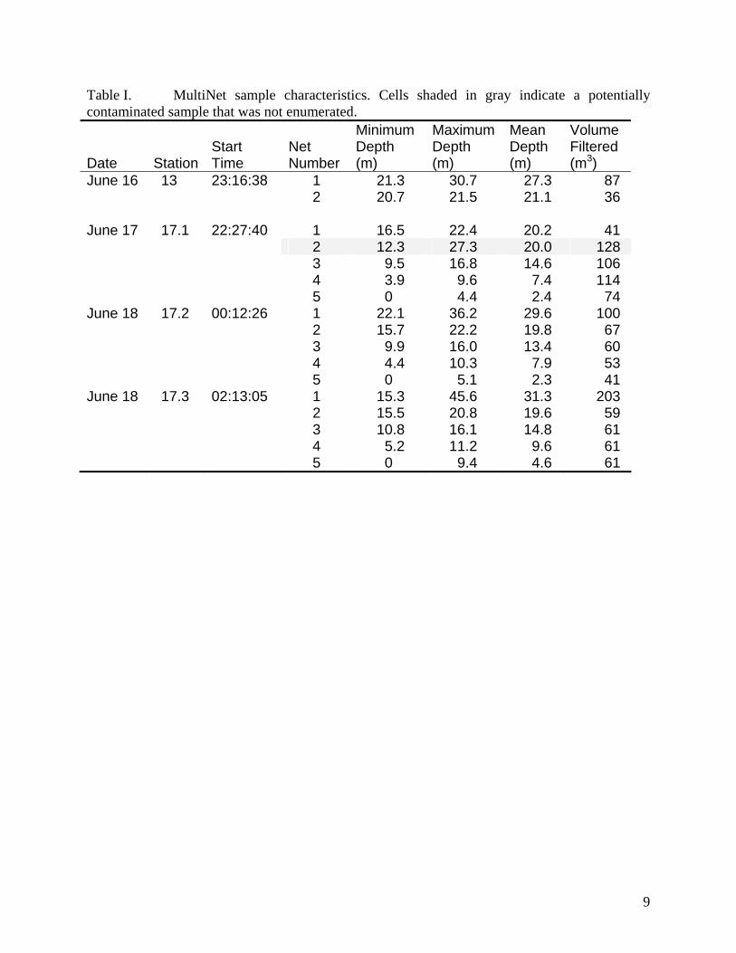
9
Table I. MultiNet sample characteristics. Cells shaded in gray indicate a potentially contaminated sample that was not enumerated. Date
Station
Start Time
Net Number
Minimum Depth (m)
Maximum Depth (m)
Mean Depth (m)
Volume Filtered (m3)
June 16 13 23:16:38 1 21.3 30.7 27.3 87 2 20.7 21.5 21.1 36 June 17 17.1 22:27:40 1 16.5 22.4 20.2 41 2 12.3 27.3 20.0 128 3 9.5 16.8 14.6 106 4 3.9 9.6 7.4 114 5 0 4.4 2.4 74 June 18 17.2 00:12:26 1 22.1 36.2 29.6 100 2 15.7 22.2 19.8 67 3 9.9 16.0 13.4 60 4 4.4 10.3 7.9 53 5 0 5.1 2.3 41 June 18 17.3 02:13:05 1 15.3 45.6 31.3 203 2 15.5 20.8 19.6 59 3 10.8 16.1 14.8 61 4 5.2 11.2 9.6 61 5 0 9.4 4.6 61

10
Figure 1. Location of zooplankton sampling stations. Station 13 was sampled on 06/16, station 17.1 was sampled on 06/17, and stations 17.2 and 17.3 were sampled on 06/18. Inset map shows the location of the study area in relation to the Aleutian Island chain.
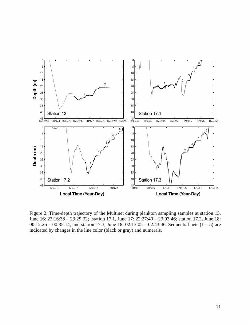
11
Figure 2. Time-depth trajectory of the Multinet during plankton sampling samples at station 13, June 16: 23:16:38 – 23:29:32; station 17.1, June 17: 22:27:40 – 23:03:46; station 17.2, June 18: 00:12:26 – 00:35:14; and station 17.3, June 18: 02:13:05 – 02:43:46. Sequential nets (1 – 5) are indicated by changes in the line color (black or gray) and numerals.

12
Figure 3. Top: An example ZooImage scan of the contents of a tissue culture tray. In this early test scan the animals near the edge of the tray were not moved away from the border as was done in subsequent scans. Insets A, B, C are enlarged in the bottom panels to show the fine detail of the scanned images of a copepod, euphausiid, and crab larva, respectively.
13
Figure 4. Comparisions of efficiency of ZooImage single target detection based on numbers of ROIs extracted from trays containing increasing densities of small targets such as copepods (left panel) and large targets such as chaetognaths (right panel). The straight line represents a 1:1 relationship between number of targets presented and the number of targets detected.

14
Figure 5. Density estimates for different taxa estimated using manual and semi-automated sample processing. This sample from a single net was a 1/64th aliquot that was first processed with ZooImage, then recombined and processed manually by observer one.

15
Figure 6. Density estimates for different taxa estimated using manual and semi-automated sample processing. This sample from a single net was a 1/64th aliquot (the same one used for results shown in the preceding figure). The sample was first processed manually by observer two and then recombined and processed with ZooImage.

16
Figure 7. Vertical distributions of dominant mesozooplankton and micronekton in the near-surface waters at four stations. Densities are plotted at the mean depth of each net fished.
Depth (m)