Honours Project Report Jordan Amos

100769796

Survey of Google’s TensorFlow

What is Tensorflow? At it’s core Tensorflow is a library for large-scale computing. It excels at performing

operations on matrices and tensors. TensorFlow’s Core API provides the ability to encode tensors and perform efficient operations in heavily optimized c++ code from a python API, and more languages are on the horizon.

This ability to compute operations on tensors is required for any machine learning or AI. TensorFlow is really trying to enable AI research and has such built several APIs that use the Core API to provide higher level access to common functions like a softmax, or an entire abstraction of a linear regression. The Learn API is has many of these high level concepts which allows for rapid development of known AI models. It allows you to focus on tweaking the hyper parameters of the model, and modeling the data.

The layout of the API and the use is such that anything on the higher layers can be implemented manually using the core APIs. The required math common across models get pushed in. This also helps ease the implementation of common networks and allows researchers to focus on the uncommon parts. We are given the freedom to experiment with individual components, and not deal with repetitive tasks.

Tensors

Tensors are the core units in tensorflow. Tensors are mappings of geometric shapes, but are really just represented as multidimensional arrays of primitive values. The number of arrays that are embedded within each other is called the rank, or order. An array ([ ]) is considered to be of rank one, an array initialized like [ ][ ] is rank 2, [ ] [ ] [ ] would be rank 3 and so on.

Tensors typically contain numbers, but aren’t limited to that on their own. A one-hot tensor is a type of encoding where one number is 1 and the rest of the numbers are zero. This type of encoding is typically used for categorical data.

The shape of the tensor is how you can represent the dimensionality of each rank of the tensor. For a tensor of rank n you could define the shape as:

shape = (dimension1, dimension2, …, dimensionn)

Sparse Tensors

One-hot encoding creates a problem with how we represent the data. Because most of the values are zero, we are storing way more information than we need to. We really only need to store the one position we care about. While categorical one-hot representations are the extreme case of this, there are many more reasons you can have a lot of zeroes in the tensor.

This problem is known as sparse data. Tensorflow provides an API called “tf.SparseTensor” that will only store the positions that are non-zero. This can relieve a lot of 1

strain on memory and processing time.

Computational Graph

The tensorflow computational graph is a graph representation of tensorflow operations that will be performed. This can also include input data in the form of placeholder operations , 2

variables , predefined operations, custom operations and more. 3

Placeholders are a promise to provide the data when the graph is run. This is typically done with the feed_dict option of an eval method. This allows you to specify operations on these values that you don’t have yet.

Variables are the core of learning in TensorFlow. The variables are the values we are modifying at each training step to maximize the effectiveness of the system. We need to define how the variables will be represented as well as an initial state. Variables have the gotcha that they need to be initialized before running. We also have tensorflow constants which can be treated like variables but will not change their value over the course of training, and do not need to be initialized.

Operations are functions typically defined in C++ that will perform the efficient computing required to modify the input tensor(s) and produce the output tensor. Each operation can accept 0-N input tensors and must return only one output tensor. This restriction allows all operations, variables, placeholders, and other tensorflow objects to be transposed and built into a graph. While this holds true at the API and infrastructure level, each operation may have some restrictions on the data formats it can work with.

Loss, or entropy, functions are a special type of operation which will return a score that says how far away from the real answer the prediction was. This implementation will depend on what exactly you are trying to represent and predict. TensorFlow provides implementations of some common loss functions such as softmax cross entropy , sigmoid cross entropy 4 5

1 https://www.tensorflow.org/api_docs/python/tf/SparseTensor 2 https://www.tensorflow.org/api_docs/python/tf/placeholder 3 https://www.tensorflow.org/api_guides/python/state_ops 4 https://www.tensorflow.org/api_docs/python/tf/nn/softmax_cross_entropy_with_logits

Optimizers are a type of operation that interacts with loss functions. They will be responsible for analyzing the result of the loss operation and adjust variables in attempt to get closer. In neural nets, optimizers are typically responsible for backpropagation. Tensorflow has some optimizers built in for various implementations, as well as a base class for implementing your own. 6

Sessions

Sessions are the interaction layer between the highly optimized C++ code and the high level python code. A session is what is responsible for passing the data, managing the graph and reporting on the response. Once a graph is built the session will be the one responsible for running it. The session can run the graph multiple times with new values each time.

Sessions enforce the separation from defining the logic of the system from the actual running of a system. This barrier prevents context switching costs, which can be expensive between the GPU and the CPU, but even worse on networked machines.

If however, you wish to perform some operation that will modify or add operations to the graph you need to use an “InteractiveSession” . 7

Standard Graph Construction

Most graphs designed for learning are constructed in a similar fashion with some variation in the structure, but some of the components are usually pretty constant. The following example is a very simple linear model. If you want to see a more detailed breakdown as well as additional getting started information view the tensorflow getting started guide. 8

First we need to import tensorflow and declare our variables. We will have a y = mx + b formula where m and b are the variables we are trying to discover. The placeholders that will hold the information we pass in will be x and y. import tensorflow as tf # linear model y = mx + b

m = tf.Variable([0.3], tf.float32) b = tf.Variable([-.3], tf.float32) x = tf.placeholder(tf.float32) y = tf.placeholder(tf.float32) Next we want to actually build the main operation that will compute the placeholders and variables the way we want. Tensorflow provides a lot of operator overloading on placeholders, variables, and tensors which makes this very easy to do. This is the part of a real

5 https://www.tensorflow.org/api_docs/python/tf/nn/sigmoid_cross_entropy_with_logits 6 https://www.tensorflow.org/api_docs/python/tf/train/Optimizer 7 https://www.tensorflow.org/api_docs/python/tf/InteractiveSession 8 https://www.tensorflow.org/get_started/get_started

implementation that will vary widely. This is a very simple example, but things can get complicated. linear_model = m * x + b # operator overloading equivalent to tf.add(tf.multiply(m,x), b) Once the y value is computed we want to see how far away from the real y we were. This is the measure of loss. We will also square the result so that we are getting distance and not direction. We also need to reduce that to a sum so that we have a single number that represents all the distances. square_difference = tf.square(linear_model - y) quadratic_loss = tf.reduce_sum(square_difference) # sum of all loss. Now that we have a loss function the next step is to add an optimizer to produce a training step. Tensorflow provides multiple optimizers, but a simple gradient descent works here. The parameter passed in is how much we want to adjust the variables on each step. optimizer = tf.train.GradientDescentOptimizer(0.01) train = optimizer.minimize(quadratic_loss) The next thing that we need to do is initialize the session. We will also need to initialize our tensorflow variables once the session is created. init = tf.global_variables_initializer() # produce init graph sess = tf.Session() # Setup session sess.run(init) # run the init graph Now that the graph is constructed, the variables are initialized and the session is ready, we can actually train our graph. Normally you would feed in a large training dataset from disk, but for simplicity we are just going to hardcode it.

for i in range(10000): # training steps # run the linear_model graph (y = 1x - 2) sess.run(train, {x: [1,2,3,4], y: [-1, 0, 1, 2]}) Now print the results of m and b to see how close to 1 and -2 you were. Usually it’s off by a rounding error. If you knew they were whole numbers you could round at the end of some training steps. print(sess.run([m, b])) The entirety of the code can be found on the following page.

import tensorflow as tf

# linear model y = mx + b

m = tf.Variable([0.3], tf.float32) b = tf.Variable([-.3], tf.float32) x = tf.placeholder(tf.float32) y = tf.placeholder(tf.float32)

linear_model = m*x + b # equivalent to tf.add(tf.multiply(m,x), b) square_difference = tf.square(linear_model - y) # equivalent to tf.square(tf.subtract(linear_model, y))

quadratic_loss = tf.reduce_sum(square_difference) # sum of all loss.

# choose optimizer

optimizer = tf.train.GradientDescentOptimizer(0.01) train = optimizer.minimize(quadratic_loss)

# need to init

init = tf.global_variables_initializer() sess = tf.Session() # Setup session sess.run(init) # run the init graph

# train the model

for i in range(10000): # training steps sess.run(train, {x: [1,2,3,4], y: [-1, 0, 1, 2]}) # run the linear_model (y = 1x - 2)

print(sess.run([m, b]))

Building With Tensorflow One of the core goals of my project was to familiarize myself with how tensorflow works

and how to build stuff with it. This section is an overview of things I built or modified in order to better understand the framework. The source code is in a separate github repo. This section will focus on the concepts behind the projects and when they are useful. This was largely based on tutorials from the tensorflow site which I will reference.

Linear Regression on MNIST This was one of the first tutorials I did and it’s an excellent exercise to get your feet wet

and start learning. The tutorial is on the tensorflow website. The basic idea is to train a linear 9

model using softmax to categorizing handwritten numbers. The dataset of handwritten numbers we are working with is a relatively famous one known as MNIST.

9 https://www.tensorflow.org/get_started/mnist/beginners

The tutorial uses similar code as provided in the intro to this report. Except switches out the to use softmax with cross entropy loss which is provided by the framework. Softmax functions are used very frequently and all they really do is squeeze values between 0 and 1. We use this as a quick proxy for probability.

The idea is to set the output variable to a single array of 10, and then flatten the image pixel array as the input variable. Since the image is 28x28 the input placeholder is 784 when flattened. This can produce results from 86~92% accuracy depending on some random initialization.

Convolutional Neural Networks on MNIST The problem with using a linear model on handwritten digits is that if someone draws

something on an angle, it won’t have the same pixel mapping. It also can’t understand if some pixels are used by multiple numbers as well, like 1 and 7. The solution to this problem is to use a system of convolution and pooling.

First published by Lawrence et al. and expanded by Krizhevsky et al. convolutional 10 11

neural networks have become the dominant AI structure in any image recognition technology. I used this technique based on the tutorial and documentation on the tensorflow site. 12

A convolutional neural network usually contains three components. A convolutional layer, a relu layer, and a pooling layer. These three layers generalize groups of pixels instead of looking at individual pixels for answers. To build a deep convolutional network, you simply stack multiple levels of these components. Each layer is called a hidden layer, so adding more increases the number of hidden layers that you have.

A convolutional layer looks uses a window to look at a smaller set of the pixels. It gives each one a score and continues along the image. Moving across the image by a number of pixels is called a stride, and the stride size is the distance moved. The pixels may not match certain pieces of an expected output or it might be skewed, but that can be picked up in the next window.

A RELU(Rectified linear unit) layer is used to make any negative values zero since they are not helpful. Since we are only negative pixel matches will occur, we want to focus on the positive matches. This also allows us to do the next step without skewing the results too far negative.

A pooling layer goes across the screen in strides and tries to pool the results into a smaller sequence. This is how each progressive hidden layer deals with a smaller set of pixels. What this allows the model to do is to provide a generalized score of how well a section matched a feature section. The smaller sections often represent things like lines or face pieces in a trained model, depending on the task. Constructing the sizes of each hidden layer will impact what features the model decides to learn in that space.

After the hidden layers there is a densely connected output layer. All the tensors are flattened into a one dimensional array. We can perform a linear regression on that densely

10 http://ieeexplore.ieee.org/abstract/document/554195/ 11 http://papers.nips.cc/paper/4824-imagenet-classification-with-deep-convolutional-neural-networks 12 https://www.tensorflow.org/get_started/mnist/pros

connected layer to give us an output. Often times people will use multiple densely connected layers to get a better result.

Through training, and backpropagation, CNNs can provide really great results. We can see greater than 99.2% result on the MNIST dataset with the code in the repo. While it’s not used in my example, implementing dropout can further improve results with a larger dataset and more training. Dropout forces the model to create multiple representations for each feature. This is valuable because having multiple representations for something allows us to understand something even if some of the key features one representation uses are missing.

This approach is really valuable in any image recognition technologies but can be used for many other things. The restriction is only that the data must be laid out in a way so that adjacent cells are more relevant than further away cells. Pixel arrays are a perfect mapping for this, since the pixels closest together form objects in the image. You can see how sound can be laid out below.

13

Multiple Linear Regression on Census Data To introduce the dataset and provide a groundwork for the next task, the tutorial on

multiple linear regression . The objective of the tutorial is to read census data and identify if a 14

person makes over or under 50k. We have a bunch of data that should have some correlation to the income. We have gender, education, relationship, work class, occupation, native country, race, age, capital gains, hours per week, and more.

To deal with the data tensorflow has a concept called bucketization . It allows us to 15

categorize by giving a continuous number representation a more meaningful categorical

13 http://brohrer.github.io/how_convolutional_neural_networks_work.html 14https://www.tensorflow.org/tutorials/wide 15 https://www.tensorflow.org/versions/r0.11/api_docs/python/contrib.training/bucketing

interval. This means our algorithm won’t need to deal with outliers or deal with linear probabilities. We can instead allow it to assign weights to the buckets which can have better correlation to the output than it would otherwise.

The other trick that this model makes use of is known as cross columns. A cross column is when a new column is introduced with both pieces of information. The model can do a linear regression on the combination of these two columns.

This type of model is particularly good at recognizing surface level linear trends. If the model can make good predictions based on a simple linear line of best fit, then this model will do really well. Where it will do poorly is when the variables interact with each other and not behave independently.

This type of approach is really useful, especially for when initially exploring a dataset and possible correlations. What makes a wide network like this even more valuable in more complex models is when we combine it with deep models, as discussed in the next section.

Wide and Deep Networks on Census Data Building on the previous implementation, a better approach would be to use both a deep

network, as well as the previous wide implementation as shown by Chen et al. To practice this 16

implementation, I worked on the tutorial from the tensorflow website on wide and deep networks. The project makes heavy use of the Layers API which can abstract a lot of neural 17 18

network layers pieces for convenience. Embedding column is a particularly interesting concept that allows us to define columns that we want to have a deep representation of along with the dimension.

The wide and deep networks work first independently to predict the result on their own. They are then passed either directly into a single densely connected layer, or first passed through their own densely connected layer. The densely connected layer uses some sort of linear softmax function to produce a probability. In training that will feed to a logistic loss function and backpropagate the results.

Deep embeddings can generalize better for any previously unseen inputs, based on previous inputs they have seen. The wider networks tend to be better at recall if a common set of conditions is a common predictor. The dichotomy is a little like memory and reasoning. The deep networks try and focus on common abstracted figures that it can work through, and the wide network is remembering important immediate indicators that don’t need much thought.

16 https://arxiv.org/abs/1606.07792 17 https://www.tensorflow.org/tutorials/wide_and_deep 18 https://www.tensorflow.org/api_guides/python/contrib.layers

Tensorflow makes this implementation really easy. The bulk of the heavy lifting is held in just a few lines of code.

m = tf.contrib.learn.DNNLinearCombinedClassifier( model_dir=model_dir, linear_feature_columns=wide_columns, dnn_feature_columns=deep_columns, dnn_hidden_units=[100, 50])

m.fit(input_fn=train_input_fn, steps=1000) results = m.evaluate(input_fn=eval_input_fn, steps=1)

The DNNLinearCombinedClassifier and the embedding columns do the majority of 19 20

the work. This is the power that tensorflow can bring to the table, when you are researching around an unfamiliar dataset, you have the full power of state of the art AI just a few lines of code away.

Word2Vec in TensorFlow The main application I am looking to explore a little deeper in my future is in NLP. Word

embeddings are a critical step towards being able to understand that. Word embeddings have been historically challenging because the data is very sparse. Later in the report you will see my further exploration on a new data set. This portion is largely based on the tutorial provided by tensorflow. 21

The first approach I looked at was a skip-gram model as introduced by Mikolov et Al . 22

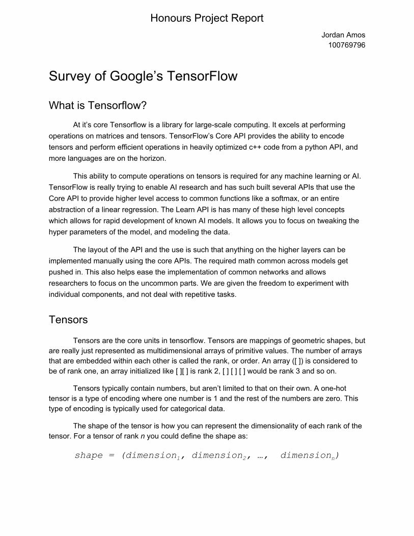
We are given a dataset known as a corpus of text and we want to try and build a model to understand word similarities. The goal is to plot out the model that we’ve trained so we can see the distances between words.

19 https://www.tensorflow.org/api_docs/python/tf/contrib/learn/DNNLinearCombinedClassifier 20 https://www.tensorflow.org/versions/master/api_docs/python/tf/contrib/layers/embedding_column 21 https://www.tensorflow.org/tutorials/word2vec 22 https://arxiv.org/abs/1301.3781

The distances between words often represent how closely they are seen together. So

when we are trying to predict the next word given some context words we can do a monte carlo average of the neighbors. This sort of model is also really good at analogical reasoning as shown by Mikolov et Al. If you ask this model king is to man as queen is to woman, the 23

resulting words often are similarly spaced apart. In this model you need a separate vector representation of the context words from the center words.

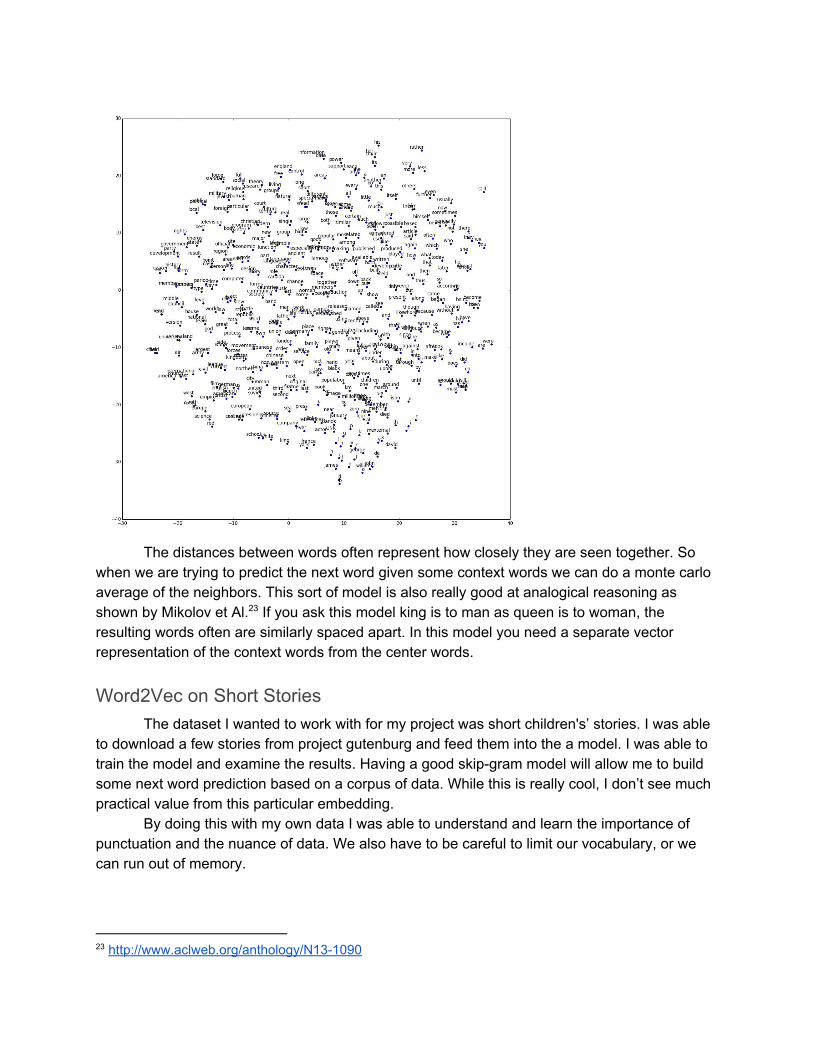
Word2Vec on Short Stories The dataset I wanted to work with for my project was short children's’ stories. I was able

to download a few stories from project gutenburg and feed them into the a model. I was able to train the model and examine the results. Having a good skip-gram model will allow me to build some next word prediction based on a corpus of data. While this is really cool, I don’t see much practical value from this particular embedding.

By doing this with my own data I was able to understand and learn the importance of punctuation and the nuance of data. We also have to be careful to limit our vocabulary, or we can run out of memory.

23 http://www.aclweb.org/anthology/N13-1090

Recurrent Neural Networks and Long Short Term Memory A Recurrent neural network is a chain of repeating simple neural network modules with a

simple internal structure like a tanh layer. The model I worked on was based on the tutorial from tensoflow and the Penn Tree Bank data . It is based on the work by Zaremba et al which 24 25 26

regularized an RNN without using dropout which is bad for RNNs. The specific type of modules used are called a Long Short Term Memory cells. They do

well in this sort of environment because they can recall older words in the context and predict the outcome. It also strives to avoid noise.

An LSTM has 4 interacting layers in the module. The module is really trying to make a decision on which data to allow through and which to hold back. It is designed to allow most things through. There is a seminal blog post by Colah that walks through how it all works and I won’t be able to do it justice. 27

The basic idea is there is a forget layer which decides which information the cells should forget. There is an input layer which decides which values we want to update. There is a tanh layer which will provide new candidate words to store in the cell state. And finally there is a densely connected output layer.

LSTM with Short Stories While I was really interested in using this model I was unable to find a way to test it

properly. I basically just reverted to using the penn tree bank data as my test set. I was happy that I got training working properly on my data, but I quickly discovered how long training one of these can take and the cycle time to learn you broke something was really bad. I also learned through this process that my radeon chipset in mac was not going to work for GPU calculations. After a lot of trying I abandoned this as a fruitless pursuit. While I am really excited that I got to learn this, I don’t think this will provide any novel functionality when paired with a short story. Sequence To Sequence machine translation

The final piece that I worked on was a machine translation as developed by Cho et al. 28

and laid out in a tutorial on the tensorflow site. The model uses two parallel RNNs typically GRU or LSTM modules. One RNN is the encoder which will process the input. The second one is a decoder and is responsible for producing the output.

The must be the same length for the RNNs so we have to use buckets and padding to make sure that we don’t run over the end. The data has the input sentence followed by a go symbol, then the desired output sentence.

24 https://www.tensorflow.org/tutorials/recurrent 25 https://catalog.ldc.upenn.edu/ldc99t42 26 https://arxiv.org/pdf/1409.2329.pdf 27 http://colah.github.io/posts/2015-08-Understanding-LSTMs/ 28 https://arxiv.org/abs/1406.1078

Short Story Bot The goal for me was to train the model to predict the next sentence in a story based on

the previos one. This would allow me to build a chatbot that could tell stories. The bot would work by making a story that pairs it with user sentences. The game goes back and forth until someone says “The End”.

The problem I ran into was encoding the data in a way that was consistent between multiple books. I was not able to get it consistently working, and it would often error during training, or worse during testing.

While this bot took forever to train, I am hopeful that I can get good results by reducing my dataset. This is the most promissing of the techniques I was exploring for my dataset and I think there’s an opportunity to make something novel. I am excited to continue working on this project going forward.

Conclusion This semester I gained a good general knowledge of AI. I was able to build a bunch of

applications and learn about a cutting edge AI framework. I am excited to pursue this field further and I was incredibly grateful for the opportunity to study it.