survey methods & design in psychology lecture 5 (2007) factor analysis 1 lecturer: james neill

Survey Methods & Design in Psychology

Lecture 5 (2007)

Factor Analysis 1

Lecturer: James Neill

Readings• Bryman, A. & Cramer, D. (1997).

Concepts and their measurement (Ch. 4).

• Fabrigar, L. R. ...[et al.]. (1999). Evaluating the use of exploratory factor analysis in psychological research.

• Tabachnick, B. G. & Fidell, L. S. (2001). Principal components and factor analysis.

• Francis 5.6

Overview

• What is FA? (purpose)

• History

• Assumptions

• Steps

• Reliability Analysis

• Creating Composite Scores

What is Factor Analysis?

• A family of techniques to examine correlations amongst variables.

• Uses correlations among many items to search for common clusters.

• Aim is to identify groups of variables which are relatively homogeneous.

• Groups of related variables are called ‘factors’.• Involves empirical testing of theoretical data

structures

Purposes

The main applications of factor analytic techniques are:

(1) to reduce the number of variables and

(2) (2) to detect structure in the relationships between variables, that is to classify variables.

Factor 1 Factor 2 Factor 3

e.g., 12 items testing might actually tap only 3 underlying factors

Conceptual Model for a Factor Analysis with a Simple Model

Conceptual Model for Factor Analysis with a Simple Model

Eysenck’s Three Personality Factors

Extraversion/introversion

Neuroticism Psychoticism

talkativeshy sociable

fun anxiousgloomy

relaxedtense

unconventionalnurturingharsh

loner

e.g., 12 items testing three underlying dimensions of personality

Conceptual Model for Factor Analysis (with cross-loadings)

Conceptual Model for Factor Analysis (3D)

Conceptual Model for Factor Analysis


Independent items

One factor

Three factors

Factor Analysis Process

• FA can be conceived of as a method for examining a matrix of correlations in search of clusters of highly correlated variables.

• A major purpose of factor analysis is data reduction, i.e., to reduce complexity in the data, by identifying underlying (latent) clusters of association.

Purpose of Factor Analysis?

History of Factor Analysis?

• Invented by Spearman (1904)

• Usage hampered by onerousness of hand calculation

• Since the advent of computers, usage has thrived, esp. to develop:• Theory

– e.g., determining the structure of personality• Practice

– e.g., development of 10,000s+ of psychological screening and measurement tests

• IQ viewed as related but separate factors, e.g,.– verbal– mathematical

• Personality viewed as 2, 3, or 5, etc. factors, e.g., the “Big 5”– Neuroticism– Extraversion– Agreeableness– Openness– Conscientiousness

Examples of Commonly Used Factor Structures in Psychology

• Six orthogonal factors, represent 76.5 % of the total variability in facial recognition.

• They are (in order of importance): 1. upper-lip2. eyebrow-position3. nose-width4. eye-position5. eye/eyebrow-length6. face-width.

Example: Factor Analysis of Essential Facial Features

Problems

Problems with factor analysis include:• Mathematically complicated • Technical vocabulary• Results usually absorb a dozen or so pages• Students do not ordinarily learn factor

analysis • Most people find the results

incomprehensible

EFA = Exploratory Factor Analysis• explores & summarises underlying

correlational structure for a data set

CFA = Confirmatory Factor Analysis• tests the correlational structure of a data

set against a hypothesised structure and rates the “goodness of fit”

Exploratory vs. Confirmatory Factor Analysis

Data Reduction 1

• FA simplifies data by revealing a smaller number of underlying factors

• FA helps to eliminate:• redundant variables • unclear variables• irrelevant variables

Steps in Factor Analysis

1. Test assumptions2. Select type of analysis

(extraction & rotation)3. Determine # of factors4. Identify which items belong in each factor5. Drop items as necessary and repeat steps

3 to 46. Name and define factors7. Examine correlations amongst factors8. Analyse internal reliability

Garbage.In.Garbage.Out

Assumption Testing – Sample Size

• Min. N of at least 5 cases per variable

• Ideal N of at least 20 cases per variable

• Total N of 200+ preferable

Assumption Testing – Sample Size

Comrey and Lee (1992):

• 50 = very poor,

• 100 = poor,

• 200 = fair,

• 300 = good,

• 500 = very good

• 1000+ = excellent

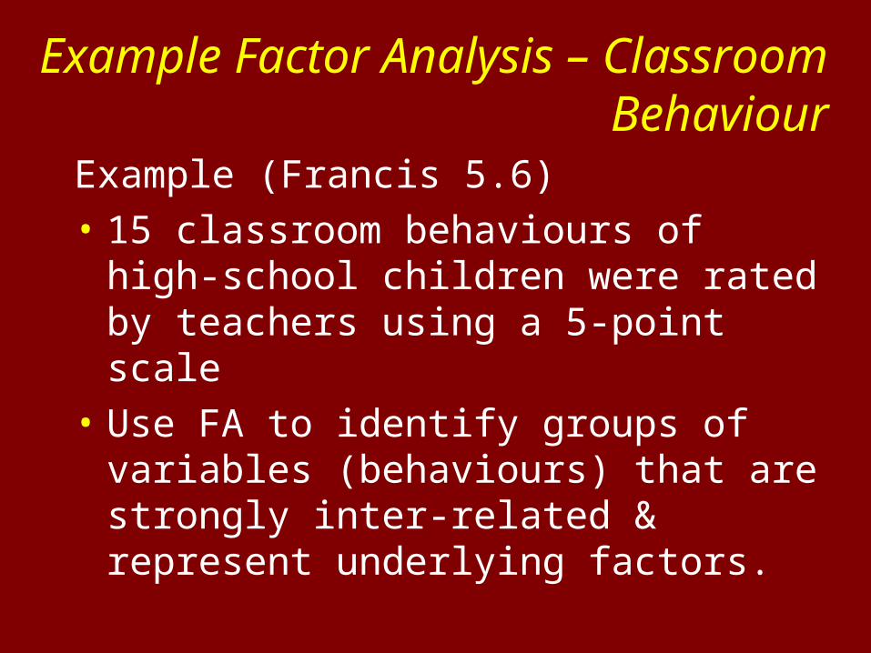
Example (Francis 5.6)

• 15 classroom behaviours of high-school children were rated by teachers using a 5-point scale

• Use FA to identify groups of variables (behaviours) that are strongly inter-related & represent underlying factors.

Example Factor Analysis – Classroom Behaviour

Classroom Behaviour Items 1

1. Cannot concentrate --- can concentrate

2. Curious & enquiring --- little curiousity

3. Perseveres --- lacks perseverance

4. Irritable --- even-tempered

5. Easily excited --- not easily excited

6. Patient --- demanding

7. Easily upset --- contented

8. Control --- no control

9. Relates warmly to others --- provocative,disruptive

10. Persistent --- easily frustrated

11. Difficult --- easy

12. Restless --- relaxed

13. Lively --- settled

14. Purposeful --- aimless

15. Cooperative --- disputes

Classroom Behaviour Items 2

Assumption Testing – LOM

• All variables must be suitable for correlational analysis, i.e., they should be ratio/metric data or at least Likert data with several interval levels.

Assumption Testing – Normality

• FA is robust to assumptions of normality(if the variables are normally distributed then the solution is enhanced)

Assumption Testing – Linearity

• Because FA is based on correlations between variables, it is important to check there are linear relations amongst the variables (i.e., check scatterplots)

Assumption Testing - Outliers

• FA is sensitive to outlying cases• Bivariate outliers

(e.g., check scatterplots)

• Multivariate outliers (e.g., Mahalanobis’ distance)

• Identify outliers, then remove or transform

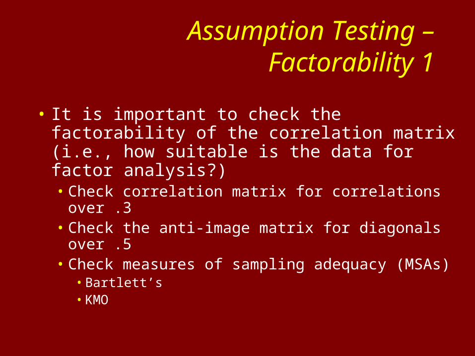
Assumption Testing – Factorability 1

• It is important to check the factorability of the correlation matrix (i.e., how suitable is the data for factor analysis?)• Check correlation matrix for correlations over .3• Check the anti-image matrix for diagonals over .5• Check measures of sampling adequacy (MSAs)

• Bartlett’s• KMO

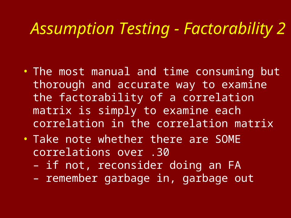
Assumption Testing - Factorability 2

• The most manual and time consuming but thorough and accurate way to examine the factorability of a correlation matrix is simply to examine each correlation in the correlation matrix

• Take note whether there are SOME correlations over .30 – if not, reconsider doing an FA– remember garbage in, garbage out

Correlation Matrix

1.000 .717 .751 .554 .429

.717 1.000 .826 .472 .262

.751 .826 1.000 .507 .311

.554 .472 .507 1.000 .610

.429 .262 .311 .610 1.000

CONCENTRATES

CURIOUS

PERSEVERES

EVEN-TEMPERED

PLACID

Correlation

CONCENTRATES CURIOUS

PERSEVERES

EVEN-TEMPERED PLACID

• Medium effort, reasonably accurate• Examine the diagonals on the anti-image

correlation matrix to assess the sampling adequacy of each variable

• Variables with diagonal anti-image correlations of less that .5 should be excluded from the analysis – they lack sufficient correlation with other variables


Anti-Image correlation matrix

concentrates

curious perserveres even-tempered

placid

concentrates .973a

curious .937a

perserveres .941a

even-tempered

.945a

placid .944a

• Quickest method, but least reliable

• Global diagnostic indicators - correlation matrix is factorable if:• Bartlett’s test of sphericity is significant and/or• Kaiser-Mayer Olkin (KMO) measure of

sampling adequacy > .5


Summary: Measures of Sampling Adequacy

• Are there several correlations over .3?

• Are the diagonals of anti-image matrix > .5?

• Is Bartlett’s test significant?• Is KMO > .5 to .6?

(depends on whose rule of thumb)

Extraction Method:PC vs. PAF

• There are two main approaches to EFA based on:– Analysing only shared variance

Principle Axis Factoring (PAF)

– Analysing all variancePrinciple Components (PC)

Principal Components (PC)

• More common

• More practical

• Used to reduce data to a set of factor scores for use in other analyses

• Analyses all the variance in each variable

Principal Components (PAF)

• Used to uncover the structure of an underlying set of p original variables

• More theoretical

• Analyses only shared variance(i.e. leaves out unique variance)

Total variance of a variable

• Often there is little difference in the solutions for the two procedures.

• Often it’s a good idea to check your solution using both techniques

• If you get a different solution between the two methods• Try to work out why and decide on which solution

is more appropriate

PC vs. PAF

Communalities - 1

• The proportion of variance in each variable which can be explained by the factors

• Communality for a variable = sum of the squared loadings for the variable on each of the factors

• Communalities range between 0 and 1• High communalities (> .5) show that the factors

extracted explain most of the variance in the variables being analysed

• Low communalities (< .5) mean there is considerable variance unexplained by the factors extracted

• May then need to extract MORE factors to explain the variance

Communalities - 2

Eigen Values

• EV = sum of squared correlations for each factor

• EV = overall strength of relationship between a factor and the variables

• Successive EVs have lower values

• Eigen values over 1 are ‘stable’

Explained Variance

• A good factor solution is one that explains the most variance with the fewest factors

• Realistically happy with 50-75% of the variance explained

How Many Factors?

A subjective process.

Seek to explain maximum variance using fewest factors, considering:

1. Theory – what is predicted/expected?

2. Eigen Values > 1? (Kaiser’s criterion)

3. Scree Plot – where does it drop off?

4. Interpretability of last factor?

5. Try several different solutions?

6. Factors must be able to be meaningfully interpreted & make theoretical sense?

How Many Factors?

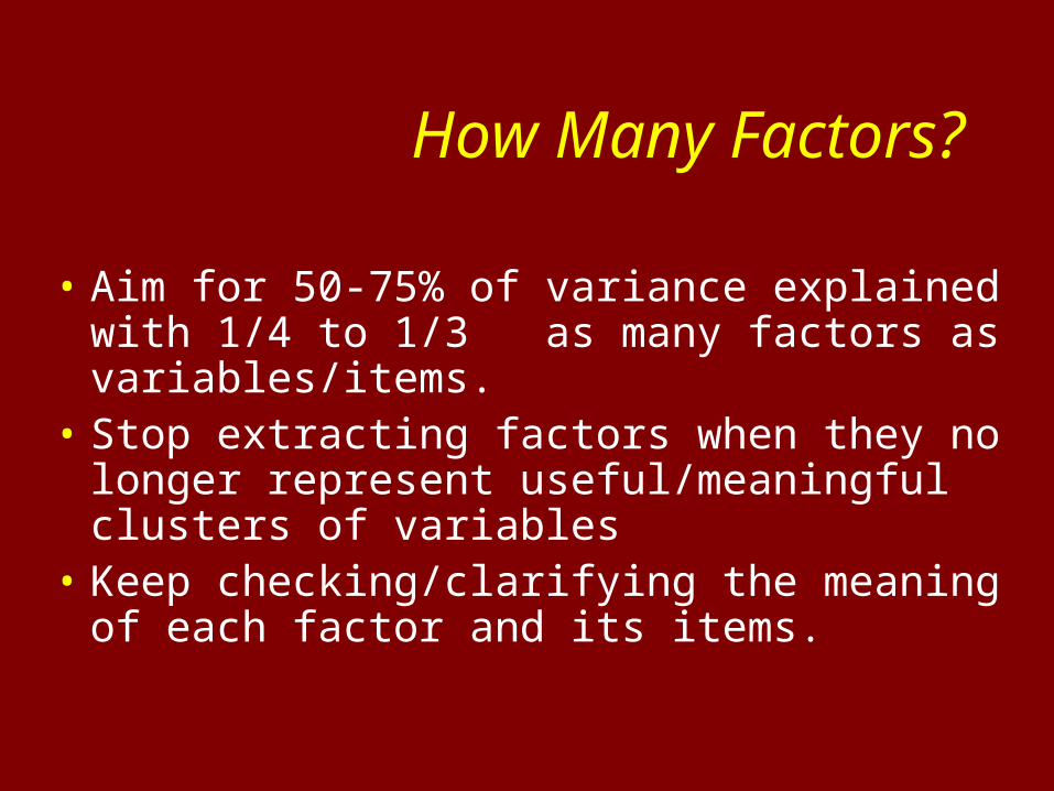
• Aim for 50-75% of variance explained with 1/4 to 1/3 as many factors as variables/items.

• Stop extracting factors when they no longer represent useful/meaningful clusters of variables

• Keep checking/clarifying the meaning of each factor and its items.

Scree Plot

• A bar graph of Eigen Values• Depicts the amount of variance explained

by each factor.• Look for point where additional factors fail

to add appreciably to the cumulative explained variance.

• 1st factor explains the most variance• Last factor explains the least amount of

variance

Scree Plot

Component Number

24

23

22

21

20

19

18

17

16

15

14

13

12

11

10

9

8

7

6

5

4

3

2

1

Eig

enva

lue

10

8

6

4

2

0

Scree Plot

• Factor loadings (FLs) indicate the relative importance of each item to each factor.

• In the initial solution, each factor tries “selfishly” to grab maximum unexplained variance.

• All variables will tend to load strongly on the 1st factor

• Factors are made up of linear combinations of the variables (max. poss. sum of squared rs for each variable)

Initial Solution - Unrotated Factor Structure 1

• 1st factor extracted:• best possible line of best fit through the original variables

• seeks to explain maximum overall variance

• a single summary of the main variance in set of items

• Each subsequent factor tries to maximise the amount of unexplained variance which it can explain.• Second factor is orthogonal to first factor - seeks to maximize

its own eigen value (i.e., tries to gobble up as much of the remaining unexplained variance as possible)


Vectors (Lines of best fit)

Initial Solution – Unrotated Factor Structure 3

• Seldom see a simple unrotated factor structure• Many variables will load on 2 or more factors• Some variables may not load highly on any

factors• Until the FLs are rotated, they are difficult to

interpret.• Rotation of the FL matrix helps to find a more

interpretable factor structure.

Rotated Component Matrixa

.861 .158 .288

.858 .310

.806 .279 .325

.778 .373 .237

.770 .376 .312

.863 .203

.259 .843 .223

.422 .756 .295

.234 .648 .526

.398 .593 .510

.328 .155 .797

.268 .286 .748

.362 .258 .724

.240 .530 .662

.405 .396 .622

PERSEVERES

CURIOUS

PURPOSEFUL ACTIVITY

CONCENTRATES

SUSTAINED ATTENTION

PLACID

CALM

RELAXED

COMPLIANT

SELF-CONTROLLED

RELATES-WARMLY

CONTENTED

COOPERATIVE

EVEN-TEMPERED

COMMUNICATIVE

1 2 3

Component

Extraction Method: Principal Component Analysis. Rotation Method: Varimax with Kaiser Normalization.

Rotation converged in 6 iterations.a.

Two Basic Types of Factor Rotation

Orthogonal(Varimax)

Oblimin

Two Basic Types of Factor Rotation

1. Orthogonalminimises factor covariation, produces factors which are uncorrelated

2. Obliminallows factors to covary, allows correlations between factors.

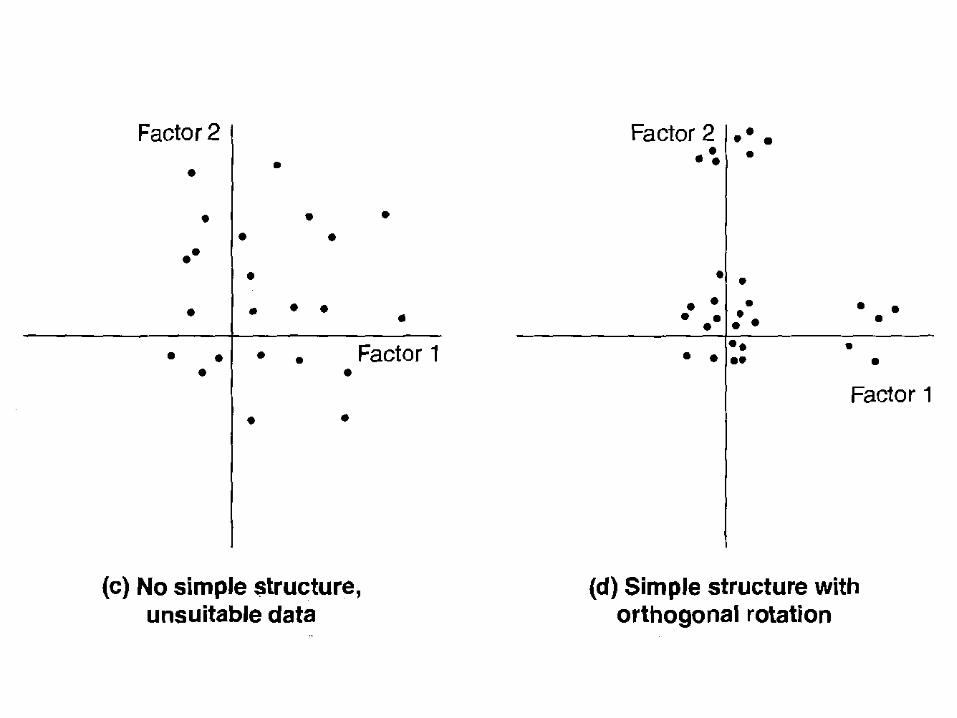
Orthogonal Rotation

Why Rotate a Factor Loading Matrix?

• After rotation, the vectors (lines of best fit) are rearranged to optimally go through clusters of shared variance

• Then the FLs and the factor they represent can be more readily interpreted

• A rotated factor structure is simpler & more easily interpretable– each variable loads strongly on only one factor– each factor shows at least 3 strong loadings– all loading are either strong or weak, no intermediate

loadings

Orthogonal versus Oblique Rotations

• Think about purpose of factor analysis

• Try both

• Consider interpretability

• Look at correlations between factors in oblique solution - if >.32 then go with oblique rotation (>10% shared variance between factors)

Pattern Matrixa

.920 .153

.845

.784 -.108

.682 -.338

.596 -.192 -.168

-.938

-.933 .171

-.839

-.831 -.201

-.788 -.181

-.902

-.131 -.841

-.314 -.686

.471 -.521

.400 -.209 -.433

RELATES-WARMLY

CONTENTED

COOPERATIVE

EVEN-TEMPERED

COMMUNICATIVE

PERSEVERES

CURIOUS

PURPOSEFUL ACTIVITY

CONCENTRATES

SUSTAINED ATTENTION

PLACID

CALM

RELAXED

COMPLIANT

SELF-CONTROLLED

1 2 3

Component

Extraction Method: Principal Component Analysis. Rotation Method: Oblimin with Kaiser Normalization.


Task Orientation

Sociability

Settledness

Pattern Matrixa

.939

.933 -.163

.835

.831 .198

.781 .185

.898

.114 .842

.302 .685

-.147 .921

.863

.795

.330 .694

.181 .173 .606

PERSEVERES

CURIOUS

PURPOSEFUL ACTIVITY

CONCENTRATES

SUSTAINED ATTENTION

PLACID

CALM

RELAXED

RELATES-WARMLY

CONTENTED

COOPERATIVE

EVEN-TEMPERED

COMMUNICATIVE

1 2 3

Component

Extraction Method: Principal Component Analysis. Rotation Method: Oblimin with Kaiser Normalization.


Factor structure is most interpretable when:1. Each variable loads strongly on only one factor2. Each factor has two or more strong loadings3. Most factor loadings are either high or low with

few of intermediate value• Loadings of +.40 or more are generally OK

Factor Structure

How do I eliminate items?

A subjective process, but consider:• Size of main loading (min=.4)• Size of cross loadings (max=.3?)• Meaning of item (face validity)• Contribution it makes to the factor• Eliminate 1 variable at a time, then re-run, before

deciding which/if any items to eliminate next• Number of items already in the factor

• More items in a factor -> greater reliability

• Minimum = 3• Maximum = unlimited• The more items, the more

rounded the measure• Law of diminishing returns• Typically = 4 to 10 is reasonable

How Many Items per Factor?

Interpretability• Must be able to understand and interpret a factor if you’re

going to extract it• Be guided by theory and common sense in selecting factor

structure• However, watch out for ‘seeing what you want to see’

when factor analysis evidence might suggest a different solution

• There may be more than one good solution, e.g.,• 2 factor model of personality• 5 factor model of personality• 16 factor model of personality

Factor Loadings & Item Selection 1

Factor structure is most interpretable when:

1. each variable loads strongly on only one factor (strong is > +.40)

2. each factor shows 3 or more strong loadings, more = greater reliability

3. most loadings are either high or low, few intermediate values

• These elements give a ‘simple’ factor structure.

Factor Loadings & Item Selection 2

• Comrey & Lee (1992)– loadings > .70 - excellent– > 63 - very good– > .55 - good– > .45 - fair– > .32 - poor

• Choosing a cut-off for acceptable loadings:– look for gap in loadings– choose cut-off because factors can be interpreted

above but not below cut-off

Example – Condom Use

• The Condom Use Self-Efficacy Scale (CUSES) was administered to 447 multicultural college students.

• PC FA with a varimax rotation.

• Three distinct factors were extracted:1. `Appropriation'

2. `Sexually Transmitted Diseases‘

3. `Partners' Disapproval.

Factor Loadings & Item Selection

Factor 1: Appropriation FL I feel confident in my ability to put a condom on myself or my partner .75

I feel confident I could purchase condoms without feeling embarrassed .65

I feel confident I could remember to carry a condom with me should I need one .61

I feel confident I could gracefully remove and dispose of a condom after sexual intercourse .56


Factor 2: STDs FL I would not feel confident suggesting using condoms with a new partner because I would be afraid he or she would think I've had a past homosexual experience .72

I would not feel confident suggesting using condoms with a new partner because I would be afraid he or she would think I have a sexually transmitted disease .86

I would not feel confident suggesting using condoms with a new partner because I would be afraid he or she would think I thought they had a sexually transmitted disease .80


Factor 3: Partner's reaction FL If I were to suggest using a condom to a partner, I would feel afraid that he or she would reject me .73

If I were unsure of my partner's feelings about using condoms I would not suggest using one .65

If my partner and I were to try to use a condom and did not succeed, I would feel embarrassed to try to use one again (e.g. not being able to unroll condom, putting it on backwards or awkwardness) .58

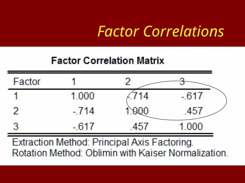
Factor Correlations

Summary 1

• Factor analysis is a family of multivariate correlational data analysis methods for summarising clusters of covariance.

Summary 2

• FA analyses and summarises correlations amongst items

• These common clusters (the factors) can be used as summary indicators of the underlying construct

Assumptions Summary 1

• 5+ cases per variables (ideal is 20 per)

• N > 200

• Outliers

• Factorability of correlation matrix

• Normality enhances the solution

Assumptions Summary 2• Communalities

• Eigen Values & % variance

• Scree Plot

• Number of factors extracted

• Rotated factor loadings

• Theoretical underpinning

Summary – Type of FA

• PC vs. PAF– PC for data reduction e.g., computing composite

scores for another analysis (uses all variance)– PAF for theoretical data exploration (uses shared

variance)– Try both ways – are solutions different?

Summary –Rotation

• Rotation– orthogonal – perpendicular vectors– oblique – angled vectors– Try both ways – are solutions different?

Factor Analysis in Practice 1

• To find a good solution, most researchers, try out each combination of– PC-varimax– PC-oblimin– PAF-varimax– PAF-oblimin

• The above methods would then be commonly tried out on a range of possible/likely factors, e.g., for 2, 3, 4, 5, 6, and 7 factors

• Try different numbers of factors• Try orthogonal & oblimin solutions• Try eliminating poor items• Conduct reliability analysis• Check factor structure across sub-groups if

sufficient data• You will probably come up with a different

solution from someone else!

Factor Analysis in Practice 2

No. of factors to extract?

• Inspect EVs - look for > 1

• % of variance explained

• Inspect scree plot

• Communalities

• Interpretability

• Theoretical reason

Summary – Factor Extraction

Beyond Factor Analysis (next week)

• Check Internal Consistency

• Create composite or factor scores

• Use composite scores in subsequent analyses (e.g., MLR, ANOVA)

• Develop new version of measurement instrument

References

• Annotated SPSS Factor Analysis outputhttp://www.ats.ucla.edu/STAT/spss/output/factor1.htm

• Further links & extra readinghttp://del.icio.us/tag/factoranalysis

http://www.ats.ucla.edu/STAT/spss/output/factor1.htm

http://www.ats.ucla.edu/STAT/spss/output/factor1.htm

http://del.icio.us/tag/factoranalysis

http://del.icio.us/tag/factoranalysis

survey methods & design in psychology lecture 5 (2007) factor analysis 1 lecturer: james neill

Documents