survey article inter-coder agreement for computational linguistics
TRANSCRIPT

Survey Article
Inter-Coder Agreement forComputational Linguistics
Ron Artstein∗
University of Essex
Massimo Poesio∗∗
University of Essex/Universita di Trento
This article is a survey of methods for measuring agreement among corpus annotators. It exposesthe mathematics and underlying assumptions of agreement coefficients, covering Krippendorff’salpha as well as Scott’s pi and Cohen’s kappa; discusses the use of coefficients in several annota-tion tasks; and argues that weighted, alpha-like coefficients, traditionally less used than kappa-like measures in computational linguistics, may be more appropriate for many corpus annotationtasks—but that their use makes the interpretation of the value of the coefficient even harder.
1. Introduction and Motivations
Since the mid 1990s, increasing effort has gone into putting semantics and discourseresearch on the same empirical footing as other areas of computational linguistics (CL).This soon led to worries about the subjectivity of the judgments required to createannotated resources, much greater for semantics and pragmatics than for the aspects oflanguage interpretation of concern in the creation of early resources such as the Browncorpus (Francis and Kucera 1982), the British National Corpus (Leech, Garside, andBryant 1994), or the Penn Treebank (Marcus, Marcinkiewicz, and Santorini 1993). Prob-lems with early proposals for assessing coders’ agreement on discourse segmentationtasks (such as Passonneau and Litman 1993) led Carletta (1996) to suggest the adoptionof the K coefficient of agreement, a variant of Cohen’s κ (Cohen 1960), as this had alreadybeen used for similar purposes in content analysis for a long time.1 Carletta’s proposals
∗ Now at the Institute for Creative Technologies, University of Southern California, 13274 Fiji Way, MarinaDel Rey, CA 90292.
∗∗ At the University of Essex: Department of Computing and Electronic Systems, University of Essex,Wivenhoe Park, Colchester, CO4 3SQ, UK. E-mail: [email protected]. At the University of Trento:CIMeC, Universita degli Studi di Trento, Palazzo Fedrigotti, Corso Bettini, 31, 38068 Rovereto (TN), Italy.E-mail: [email protected].
1 The literature is full of terminological inconsistencies. Carletta calls the coefficient of agreement sheargues for “kappa,” referring to Krippendorff (1980) and Siegel and Castellan (1988), and using Siegeland Castellan’s terminology and definitions. However, Siegel and Castellan’s statistic, which they call K,is actually Fleiss’s generalization to more than two coders of Scott’s π, not of the original Cohen’s κ; toconfuse matters further, Siegel and Castellan use the Greek letter κ to indicate the parameter which isestimated by K. In what follows, we use κ to indicate Cohen’s original coefficient and its generalizationto more than two coders, and K for the coefficient discussed by Siegel and Castellan.
Submission received: 26 August 2005; revised submission received: 21 December 2007; accepted forpublication: 28 January 2008.
© 2008 Association for Computational Linguistics

Computational Linguistics Volume 34, Number 4
were enormously influential, and K quickly became the de facto standard for measuringagreement in computational linguistics not only in work on discourse (Carletta et al.1997; Core and Allen 1997; Hearst 1997; Poesio and Vieira 1998; Di Eugenio 2000; Stolckeet al. 2000; Carlson, Marcu, and Okurowski 2003) but also for other annotation tasks(e.g., Veronis 1998; Bruce and Wiebe 1998; Stevenson and Gaizauskas 2000; Craggs andMcGee Wood 2004; Mieskes and Strube 2006). During this period, however, a numberof questions have also been raised about K and similar coefficients—some already inCarletta’s own work (Carletta et al. 1997)—ranging from simple questions about theway the coefficient is computed (e.g., whether it is really applicable when more thantwo coders are used), to debates about which levels of agreement can be considered‘acceptable’ (Di Eugenio 2000; Craggs and McGee Wood 2005), to the realization that Kis not appropriate for all types of agreement (Poesio and Vieira 1998; Marcu, Romera,and Amorrortu 1999; Di Eugenio 2000; Stevenson and Gaizauskas 2000). Di Eugenioraised the issue of the effect of skewed distributions on the value of K and pointed outthat the original κ developed by Cohen is based on very different assumptions aboutcoder bias from the K of Siegel and Castellan (1988), which is typically used in CL. Thisissue of annotator bias was further debated in Di Eugenio and Glass (2004) and CraggsandMcGeeWood (2005). Di Eugenio andGlass pointed out that the choice of calculatingchance agreement by using individual coder marginals (κ) or pooled distributions (K)can lead to reliability values falling on different sides of the accepted 0.67 threshold,and recommended reporting both values. Craggs and McGee Wood argued, followingKrippendorff (2004a,b), that measures like Cohen’s κ are inappropriate for measur-ing agreement. Finally, Passonneau has been advocating the use of Krippendorff’s α(Krippendorff 1980, 2004a) for coding tasks in CL which do not involve nominal anddisjoint categories, including anaphoric annotation, wordsense tagging, and summa-rization (Passonneau 2004, 2006; Nenkova and Passonneau 2004; Passonneau, Habash,and Rambow 2006).
Now that more than ten years have passed since Carletta’s original presentationat the workshop on Empirical Methods in Discourse, it is time to reconsider the useof coefficients of agreement in CL in a systematic way. In this article, a survey ofcoefficients of agreement and their use in CL, we have threemain goals. First, we discussin some detail the mathematics and underlying assumptions of the coefficients used ormentioned in the CL and content analysis literatures. Second, we also cover in somedetail Krippendorff’s α, often mentioned but never really discussed in detail in previousCL literature other than in the papers by Passonneau just mentioned. Third, we reviewthe past ten years of experience with coefficients of agreement in CL, reconsidering theissues that have been raised also from a mathematical perspective.2
2. Coefficients of Agreement
2.1 Agreement, Reliability, and Validity
We begin with a quick recap of the goals of agreement studies, inspired by Krippendorff(2004a, Section 11.1). Researchers who wish to use hand-coded data—that is, data inwhich items are labeled with categories, whether to support an empirical claim or todevelop and test a computational model—need to show that such data are reliable.
2 Only part of our material could fit in this article. An extended version of the survey is available fromhttp://cswww.essex.ac.uk/Research/nle/arrau/.
556
Artstein and Poesio Inter-Coder Agreement for CL
The fundamental assumption behind the methodologies discussed in this article is thatdata are reliable if coders can be shown to agree on the categories assigned to units toan extent determined by the purposes of the study (Krippendorff 2004a; Craggs andMcGeeWood 2005). If different coders produce consistently similar results, then we caninfer that they have internalized a similar understanding of the annotation guidelines,and we can expect them to perform consistently under this understanding.
Reliability is thus a prerequisite for demonstrating the validity of the codingscheme—that is, to show that the coding scheme captures the “truth” of the phenom-enon being studied, in case this matters: If the annotators are not consistent then eithersome of them are wrong or else the annotation scheme is inappropriate for the data.(Just as in real life, the fact that witnesses to an event disagree with each other makes itdifficult for third parties to know what actually happened.) However, it is important tokeep in mind that achieving good agreement cannot ensure validity: Two observers ofthe same event may well share the same prejudice while still being objectively wrong.
2.2 A Common Notation
It is useful to think of a reliability study as involving a set of items (markables), aset of categories, and a set of coders (annotators) who assign to each item a uniquecategory label. The discussions of reliability in the literature often use different notationsto express these concepts. We introduce a uniform notation, which we hope will makethe relations between the different coefficients of agreement clearer.
• The set of items is { i | i ∈ I } and is of cardinality i.
• The set of categories is { k | k ∈ K } and is of cardinality k.
• The set of coders is { c | c ∈ C } and is of cardinality c.
Confusion also arises from the use of the letter P, which is used in the literature with atleast three distinct interpretations, namely “proportion,” “percent,” and “probability.”We will use the following notation uniformly throughout the article.
• Ao is observed agreement and Do is observed disagreement.
• Ae and De are expected agreement and expected disagreement,respectively. The relevant coefficient will be indicated with a superscriptwhen an ambiguity may arise (for example, Aπ
e is the expected agreementused for calculating π, and Aκ
e is the expected agreement used forcalculating κ).
• P(·) is reserved for the probability of a variable, and P(·) is an estimate ofsuch probability from observed data.
Finally, we use n with a subscript to indicate the number of judgments of a given type:
• nik is the number of coders who assigned item i to category k;
• nck is the number of items assigned by coder c to category k;
• nk is the total number of items assigned by all coders to category k.
557
Computational Linguistics Volume 34, Number 4
2.3 Agreement Without Chance Correction
The simplest measure of agreement between two coders is percentage of agreement orobserved agreement, defined for example by Scott (1955, page 323) as “the percentage ofjudgments on which the two analysts agree when coding the same data independently.”This is the number of items on which the coders agree divided by the total numberof items. More precisely, and looking ahead to the following discussion, observedagreement is the arithmetic mean of the agreement value agri for all items i ∈ I, definedas follows:
agri ={1 if the two coders assign i to the same category0 if the two coders assign i to different categories
Observed agreement over the values agri for all items i ∈ I is then:
Ao =1i ∑
i∈I
agri
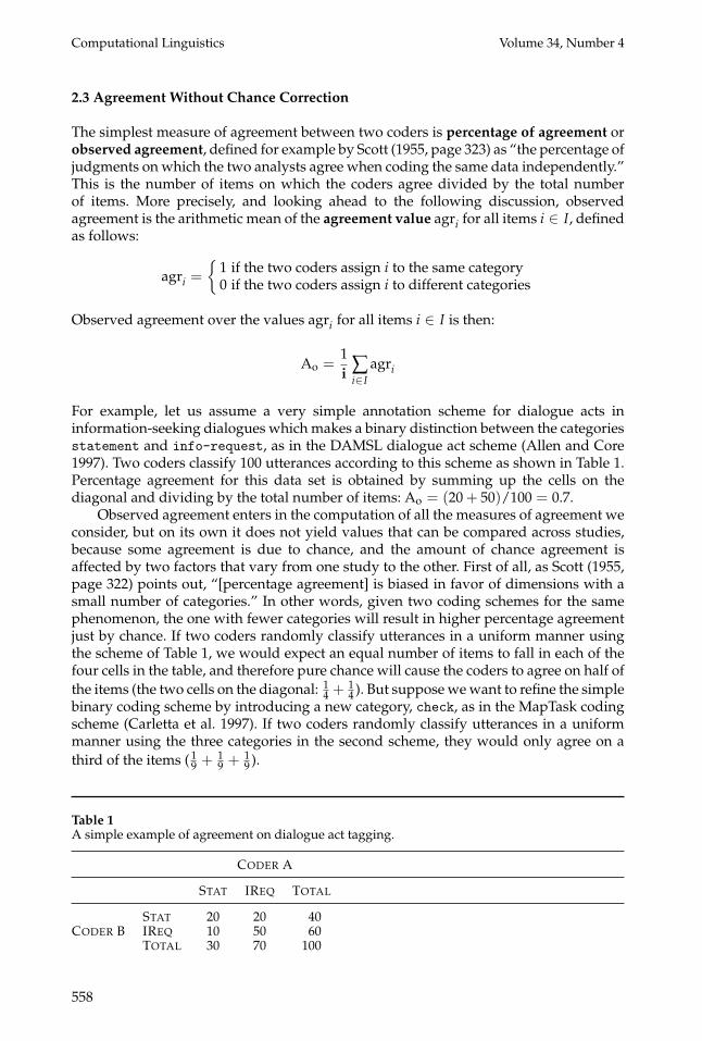
For example, let us assume a very simple annotation scheme for dialogue acts ininformation-seeking dialogues which makes a binary distinction between the categoriesstatement and info-request, as in the DAMSL dialogue act scheme (Allen and Core1997). Two coders classify 100 utterances according to this scheme as shown in Table 1.Percentage agreement for this data set is obtained by summing up the cells on thediagonal and dividing by the total number of items: Ao = (20+ 50)/100 = 0.7.
Observed agreement enters in the computation of all the measures of agreement weconsider, but on its own it does not yield values that can be compared across studies,because some agreement is due to chance, and the amount of chance agreement isaffected by two factors that vary from one study to the other. First of all, as Scott (1955,page 322) points out, “[percentage agreement] is biased in favor of dimensions with asmall number of categories.” In other words, given two coding schemes for the samephenomenon, the one with fewer categories will result in higher percentage agreementjust by chance. If two coders randomly classify utterances in a uniform manner usingthe scheme of Table 1, we would expect an equal number of items to fall in each of thefour cells in the table, and therefore pure chance will cause the coders to agree on half ofthe items (the two cells on the diagonal: 14 + 1
4 ). But suppose wewant to refine the simplebinary coding scheme by introducing a new category, check, as in the MapTask codingscheme (Carletta et al. 1997). If two coders randomly classify utterances in a uniformmanner using the three categories in the second scheme, they would only agree on athird of the items (19 + 1
9 + 19 ).
Table 1A simple example of agreement on dialogue act tagging.
CODER A
STAT IREQ TOTAL
STAT 20 20 40CODER B IREQ 10 50 60
TOTAL 30 70 100
558

Artstein and Poesio Inter-Coder Agreement for CL
The second reason percentage agreement cannot be trusted is that it does notcorrect for the distribution of items among categories: We expect a higher percentageagreement when one category is much more common than the other. This problem,already raised by Hsu and Field (2003, page 207) among others, can be illustratedusing the following example (Di Eugenio and Glass 2004, example 3, pages 98–99).Suppose 95% of utterances in a particular domain are statement, and only 5% are info-request. We would then expect by chance that 0.95× 0.95 = 0.9025 of the utteranceswould be classified as statement by both coders, and 0.05 × 0.05 = 0.0025 as info-request, so the coders would agree on 90.5% of the utterances. Under such circum-stances, a seemingly high observed agreement of 90% is actually worse than expected bychance.
The conclusion reached in the literature is that in order to get figures that are compa-rable across studies, observed agreement has to be adjusted for chance agreement. Theseare the measures we will review in the remainder of this article. We will not look at thevariants of percentage agreement used in CL work on discourse before the introductionof kappa, such as percentage agreement with an expert and percentage agreement withthe majority; see Carletta (1996) for discussion and criticism.3
2.4 Chance-Corrected Coefficients for Measuring Agreement between Two Coders
All of the coefficients of agreement discussed in this article correct for chance on thebasis of the same idea. First we find how much agreement is expected by chance: Let uscall this value Ae. The value 1−Ae will then measure how much agreement over andabove chance is attainable; the value Ao −Ae will tell us how much agreement beyondchance was actually found. The ratio between Ao−Ae and 1−Ae will then tell us whichproportion of the possible agreement beyond chance was actually observed. This ideais expressed by the following formula.
S,π, κ =Ao −Ae
1−Ae
The three best-known coefficients, S (Bennett, Alpert, and Goldstein 1954), π (Scott1955), and κ (Cohen 1960), and their generalizations, all use this formula; whereasKrippendorff’s α is based on a related formula expressed in terms of disagreement(see Section 2.6). All three coefficients therefore yield values of agreement between−Ae/1−Ae (no observed agreement) and 1 (observed agreement = 1), with the value 0signifying chance agreement (observed agreement = expected agreement). Note alsothat whenever agreement is less than perfect (Ao < 1), chance-corrected agreementwill be strictly lower than observed agreement, because some amount of agreementis always expected by chance.
Observed agreement Ao is easy to compute, and is the same for all threecoefficients—the proportion of items on which the two coders agree. But the notionof chance agreement, or the probability that two coders will classify an arbitrary itemas belonging to the same category by chance, requires a model of what would happenif coders’ behavior was only by chance. All three coefficients assume independence ofthe two coders—that is, that the chance of c1 and c2 agreeing on any given category k
3 The extended version of the article also includes a discussion of why χ2 and correlation coefficients arenot appropriate for this task.
559

Computational Linguistics Volume 34, Number 4
Table 2The value of different coefficients applied to the data from Table 1.
Coefficient Expected agreement Chance-corrected agreement
S 2× ( 12 )2 = 0.5 (0.7− 0.5)/(1− 0.5) = 0.4
π 0.352 + 0.652 = 0.545 (0.7− 0.545)/(1− 0.545) ≈ 0.341κ 0.3× 0.4+ 0.6× 0.7 = 0.54 (0.7− 0.54)/(1− 0.54) ≈ 0.348
Observed agreement for all the coefficients is 0.7.
is the product of the chance of each of them assigning an item to that category:P(k|c1) · P(k|c2).4 Expected agreement is then the probability of c1 and c2 agreeing onany category, that is, the sum of the product over all categories:
ASe = Aπ
e = Aκe = ∑
k∈K
P(k|c1) · P(k|c2)
The difference between S, π, and κ lies in the assumptions leading to the calculation ofP(k|ci), the chance that coder ci will assign an arbitrary item to category k (Zwick 1988;Hsu and Field 2003).
S: This coefficient is based on the assumption that if coders were operatingby chance alone, we would get a uniform distribution: That is, for any twocoders cm, cn and any two categories kj, kl , P(kj|cm) = P(kl |cn).
π: If coders were operating by chance alone, we would get the samedistribution for each coder: For any two coders cm, cn and any category k,P(k|cm) = P(k|cn).
κ: If coders were operating by chance alone, we would get a separatedistribution for each coder.
Additionally, the lack of independent prior knowledge of the distribution of itemsamong categories means that the distribution of categories (for π) and the priors for theindividual coders (for κ) have to be estimated from the observed data. Table 2 demon-strates the effect of the different chance models on the coefficient values. The remainderof this section explains how the three coefficients are calculated when the reliability datacome from two coders; we will discuss a variety of proposed generalizations starting inSection 2.5.
2.4.1 All Categories Are Equally Likely: S. The simplest way of discounting for chanceis the one adopted to compute the coefficient S (Bennett, Alpert, and Goldstein 1954),also known in the literature as C, κn, G, and RE (see Zwick 1988; Hsu and Field 2003).As noted previously, the computation of S is based on an interpretation of chance asa random choice of category from a uniform distribution—that is, all categories areequally likely. If coders classify the items into k categories, then the chance P(k|ci) of
4 The independence assumption has been the subject of much criticism, for example by John S. Uebersax.http://ourworld.compuserve.com/homepages/jsuebersax/agree.htm.
560

Artstein and Poesio Inter-Coder Agreement for CL
any coder assigning an item to category k under the uniformity assumption is 1k ; hence
the total agreement expected by chance is
ASe = ∑
k∈K
1k·1k
= k ·(1k
)2
=1k
The calculation of the value of S for the figures in Table 1 is shown in Table 2.The coefficient S is problematic in many respects. The value of the coefficient can
be artificially increased simply by adding spurious categories which the coders wouldnever use (Scott 1955, pages 322–323). In the case of CL, for example, S would rewarddesigning extremely fine-grained tagsets, provided that most tags are never actuallyencountered in real data. Additional limitations are noted byHsu and Field (2003). It hasbeen argued that uniformity is the best model for a chance distribution of items amongcategories if we have no independent prior knowledge of the distribution (Brennan andPrediger 1981). However, a lack of prior knowledge does not mean that the distributioncannot be estimated post hoc, and this is what the other coefficients do.
2.4.2 A Single Distribution: π. All of the other methods for discounting chance agreementwe discuss in this article attempt to overcome the limitations of S’s strong uniformityassumption using an idea first proposed by Scott (1955): Use the actual behavior of thecoders to estimate the prior distribution of the categories. As noted earlier, Scott basedhis characterization of π on the assumption that random assignment of categories toitems, by any coder, is governed by the distribution of items among categories in theactual world. The best estimate of this distribution is P(k), the observed proportion ofitems assigned to category k by both coders.
P(k|c1) = P(k|c2) = P(k)
P(k), the observed proportion of items assigned to category k by both coders, is thetotal number of assignments to k by both coders nk, divided by the overall number ofassignments, which for the two-coder case is twice the number of items i:
P(k) =nk
2i
Given the assumption that coders act independently, expected agreement is computedas follows.
Aπe = ∑
k∈K
P(k) · P(k) = ∑k∈K
(nk
2i
)2=
14i2 ∑
k∈K
n2k
It is easy to show that for any set of coding data, Aπe ≥ AS
e and therefore π ≤ S, withthe limiting case (equality) obtaining when the observed distribution of items amongcategories is uniform.
2.4.3 Individual Coder Distributions: κ. The method proposed by Cohen (1960) to calcu-late expected agreement Ae in his κ coefficient assumes that random assignment ofcategories to items is governed by prior distributions that are unique to each coder,and which reflect individual annotator bias. An individual coder’s prior distribution is
561
Computational Linguistics Volume 34, Number 4
estimated by looking at her actual distribution: P(k|ci), the probability that coder ci willclassify an arbitrary item into category k, is estimated by using P(k|ci), the proportionof items actually assigned by coder ci to category k; this is the number of assignmentsto k by ci, ncik, divided by the number of items i.
P(k|ci) = P(k|ci) =ncik
i
As in the case of S and π, the probability that the two coders c1 and c2 assign an item toa particular category k ∈ K is the joint probability of each coder making this assignmentindependently. For κ this joint probability is P(k|c1) · P(k|c2); expected agreement is thenthe sum of this joint probability over all the categories k ∈ K.
Aκe = ∑
k∈K
P(k|c1) · P(k|c2) = ∑k∈K
nc1k
i·nc2k
i=
1i2 ∑
k∈K
nc1knc2k
It is easy to show that for any set of coding data, Aπe ≥ Aκ
e and therefore π ≤ κ, with thelimiting case (equality) obtaining when the observed distributions of the two coders areidentical. The relationship between κ and S is not fixed.
2.5 More Than Two Coders
In corpus annotation practice, measuring reliability with only two coders is seldomconsidered enough, except for small-scale studies. Sometimes researchers run reliabilitystudies with more than two coders, measure agreement separately for each pair ofcoders, and report the average. However, a better practice is to use generalized versionsof the coefficients. A generalization of Scott’s π is proposed in Fleiss (1971), and ageneralization of Cohen’s κ is given in Davies and Fleiss (1982). We will call thesecoefficients multi-π and multi-κ, respectively, dropping the multi-prefixes when noconfusion is expected to arise.5
2.5.1 Fleiss’s Multi-π. With more than two coders, the observed agreement Ao can nolonger be defined as the percentage of items on which there is agreement, becauseinevitably there will be items on which some coders agree and others disagree. Thesolution proposed in the literature is to measure pairwise agreement (Fleiss 1971):Define the amount of agreement on a particular item as the proportion of agreeingjudgment pairs out of the total number of judgment pairs for that item.
Multiple coders also pose a problem for the visualization of the data. When thenumber of coders c is greater than two, judgments cannot be shown in a contingencytable like Table 1, because each coder has to be represented in a separate dimension.
5 Due to historical accident, the terminology in the literature is confusing. Fleiss (1971) proposed acoefficient of agreement for multiple coders and called it κ, even though it calculates expected agreementbased on the cumulative distribution of judgments by all coders and is thus better thought of as ageneralization of Scott’s π. This unfortunate choice of name was the cause of much confusion insubsequent literature: Often, studies which claim to give a generalization of κ to more than two codersactually report Fleiss’s coefficient (e.g., Bartko and Carpenter 1976; Siegel and Castellan 1988; Di Eugenioand Glass 2004). Since Carletta (1996) introduced reliability to the CL community based on the definitionsof Siegel and Castellan (1988), the term “kappa” has been usually associated in this community withSiegel and Castellan’s K, which is in effect Fleiss’s coefficient, that is, a generalization of Scott’s π.
562

Artstein and Poesio Inter-Coder Agreement for CL
Fleiss (1971) therefore uses a different type of table which lists each item with the num-ber of judgments it received for each category; Siegel and Castellan (1988) use a similartable, which Di Eugenio and Glass (2004) call an agreement table. Table 3 is an exampleof an agreement table, in which the same 100 utterances from Table 1 are labeled bythree coders instead of two. Di Eugenio and Glass (page 97) note that compared tocontingency tables like Table 1, agreement tables like Table 3 lose information becausethey do not say which coder gave each judgment. This information is not used in thecalculation of π, but is necessary for determining the individual coders’ distributions inthe calculation of κ. (Agreement tables also add information compared to contingencytables, namely, the identity of the items that make up each contingency class, but thisinformation is not used in the calculation of either κ or π.)
Let nik stand for the number of times an item i is classified in category k (i.e., thenumber of coders that make such a judgment): For example, given the distribution inTable 3, nUtt1Stat = 2 and nUtt1IReq = 1. Each category k contributes (nik
2 ) pairs of agreeingjudgments for item i; the amount of agreement agri for item i is the sum of (nik
2 ) over allcategories k ∈ K, divided by (c2), the total number of judgment pairs per item.
agri =1
(c2)∑k∈K
(nik
2
)=
1c(c− 1) ∑
k∈K
nik(nik − 1)
For example, given the results in Table 3, we find the agreement value for Utterance 1as follows.
agr1 =1
(32)
((nUtt1Stat
2
)+
(nUtt1IReq
2
))=
13
(1+ 0) ≈ 0.33
The overall observed agreement is the mean of agri for all items i ∈ I.
Ao =1i ∑
i∈I
agri =1
ic(c− 1) ∑i∈I
∑k∈K
nik(nik − 1)
(Notice that this definition of observed agreement is equivalent to the mean of thetwo-coder observed agreement values from Section 2.4 for all coder pairs.)
If observed agreement is measured on the basis of pairwise agreement (the pro-portion of agreeing judgment pairs), it makes sense to measure expected agreement interms of pairwise comparisons as well, that is, as the probability that any pair of judg-ments for an item would be in agreement—or, said otherwise, the probability that two
Table 3Agreement table with three coders.
STAT IREQ
Utt1 2 1Utt2 0 3...
Utt100 1 2
TOTAL 90 (0.3) 210 (0.7)
563

Computational Linguistics Volume 34, Number 4
arbitrary coders would make the same judgment for a particular item by chance. This isthe approach taken by Fleiss (1971). Like Scott, Fleiss interprets “chance agreement” asthe agreement expected on the basis of a single distribution which reflects the combinedjudgments of all coders, meaning that expected agreement is calculated using P(k), theoverall proportion of items assigned to category k, which is the total number of suchassignments by all coders nk divided by the overall number of assignments. The latter,in turn, is the number of items imultiplied by the number of coders c.
P(k) =1icnk
As in the two-coder case, the probability that two arbitrary coders assign an item to aparticular category k ∈ K is assumed to be the joint probability of each coder makingthis assignment independently, that is (P(k))2. The expected agreement is the sum ofthis joint probability over all the categories k ∈ K.
Aπe = ∑
k∈K
(P(k)
)2= ∑
k∈K
(1icnk
)2
=1
(ic)2 ∑k∈K
n2k
Multi-π is the coefficient that Siegel and Castellan (1988) call K.
2.5.2 Multi-κ. It is fairly straightforward to adapt Fleiss’s proposal to generalizeCohen’s κ proper to more than two coders, calculating expected agreement based onindividual coder marginals. A detailed proposal can be found in Davies and Fleiss(1982), or in the extended version of this article.
2.6 Krippendorff’s α and Other Weighted Agreement Coefficients
A serious limitation of both π and κ is that all disagreements are treated equally. Butespecially for semantic and pragmatic features, disagreements are not all alike. Even forthe relatively simple case of dialogue act tagging, a disagreement between an acceptand a reject interpretation of an utterance is clearly more serious than a disagreementbetween an info-request and a check. For tasks such as anaphora resolution, wherereliability is determined by measuring agreement on sets (coreference chains), allowingfor degrees of disagreement becomes essential (see Section 4.4). Under such circum-stances, π and κ are not very useful.
In this section we discuss two coefficients that make it possible to differentiatebetween types of disagreements: α (Krippendorff 1980, 2004a), which is a coefficientdefined in a general way that is appropriate for use with multiple coders, differentmagnitudes of disagreement, and missing values, and is based on assumptions similarto those of π; and weighted kappa κw (Cohen 1968), a generalization of κ.
2.6.1 Krippendorff’s α. The coefficient α (Krippendorff 1980, 2004a) is an extremely ver-satile agreement coefficient based on assumptions similar to π, namely, that expectedagreement is calculated by looking at the overall distribution of judgments withoutregard to which coders produced these judgments. It applies to multiple coders, andit allows for different magnitudes of disagreement. When all disagreements are con-sidered equal it is nearly identical to multi-π, correcting for small sample sizes byusing an unbiased estimator for expected agreement. In this section we will present
564

Artstein and Poesio Inter-Coder Agreement for CL
Krippendorff’s α and relate it to the other coefficients discussed in this article, but wewill start with α’s origins as a measure of variance, following a long tradition of usingvariance to measure reliability (see citations in Rajaratnam 1960; Krippendorff 1970).
A sample’s variance s2 is defined as the sum of square differences from the meanSS = ∑(x − x)2 divided by the degrees of freedom df . Variance is a useful way oflooking at agreement if coders assign numerical values to the items, as in magnitudeestimation tasks. Each item in a reliability study can be considered a separate levelin a single-factor analysis of variance: The smaller the variance around each level, thehigher the reliability. When agreement is perfect, the variance within the levels (s2within)is zero; when agreement is at chance, the variance within the levels is equal to thevariance between the levels, in which case it is also equal to the overall variance of thedata: s2within = s2between = s2total. The ratios s2within/s2between (that is, 1/F) and s2within/s2total aretherefore 0 when agreement is perfect and 1 when agreement is at chance. Additionally,the latter ratio is bounded at 2: SSwithin ≤ SStotal by definition, and df total < 2 df withinbecause each item has at least two judgments. Subtracting the ratio s2within/s2total from 1yields a coefficient which ranges between−1 and 1, where 1 signifies perfect agreementand 0 signifies chance agreement.
α = 1−s2within
s2total
= 1−SSwithin/df within
SStotal/df total
We can unpack the formula for α to bring it to a form which is similar to the othercoefficients we have looked at, and which will allow generalizing α beyond simplenumerical values. The first step is to get rid of the notion of arithmetic meanwhich lies atthe heart of the measure of variance. We observe that for any set of numbers x1, . . . , xNwith a mean x = 1
N ∑Nn=1 xn, the sum of square differences from the mean SS can be
expressed as the sum of square of differences between all the (ordered) pairs of numbers,scaled by a factor of 1/2N.
SS =N
∑n=1
(xn − x)2 =12N
N
∑n=1
N
∑m=1
(xn − xm)2
For calculating α we considered each item to be a separate level in an analysis ofvariance; the number of levels is thus the number of items i, and because each codermarks each item, the number of observations for each item is the number of coders c.Within-level variance is the sum of the square differences from the mean of each item,SSwithin = ∑i ∑c(xic − xi)2, divided by the degrees of freedom df within = i(c − 1). Wecan express this as the sum of the squares of the differences between all of the judgmentpairs for each item, summed over all items and scaled by the appropriate factor. We usethe notation xic for the value given by coder c to item i, and xi for the mean of all thevalues given to item i.
s2within =SSwithin
df within=
1i(c− 1) ∑
i∈I∑c∈C
(xic − xi)2 =
12ic(c− 1) ∑
i∈I
c
∑m=1
c
∑n=1
(xicm − xicn)2
The total variance is the sum of the square differences of all judgments from the grandmean, SStotal = ∑i ∑c(xic − x)2, divided by the degrees of freedom df total = ic− 1. This
565

Computational Linguistics Volume 34, Number 4
can be expressed as the sum of the squares of the differences between all of the judg-ments pairs without regard to items, again scaled by the appropriate factor. The notationx is the overall mean of all the judgments in the data.
s2total =SStotal
df total=
1ic− 1 ∑
i∈I∑c∈C
(xic − x)2 =1
2ic(ic− 1)
i
∑j=1
c
∑m=1
i
∑l=1
c
∑n=1
(xijcm − xil cn)2
Now that we have removed references tomeans from our formulas, we can abstract overthe measure of variance. We define a distance function d which takes two numbers andreturns the square of their difference.
dab = (a − b)2
We also simplify the computation by counting all the identical value assignmentstogether. Each unique value used by the coders will be considered a category k ∈ K.We use nik for the number of times item i is given the value k, that is, the number ofcoders that make such a judgment. For every (ordered) pair of distinct values ka, kb ∈ Kthere are nikanikb
pairs of judgments of item i, whereas for non-distinct values thereare nika(nika − 1) pairs. We use this notation to rewrite the formula for the within-levelvariance. Dα
o, the observed disagreement for α, is defined as twice the variance withinthe levels in order to get rid of the factor 2 in the denominator; we also simplify theformula by using the multiplier nikanika for identical categories—this is allowed becausedkk = 0 for all k.
Dαo = 2 s2within =
1ic(c− 1) ∑
i∈I
k
∑j=1
k
∑l=1
nikjnikl
dkjkl
We perform the same simplification for the total variance, where nk stands for thetotal number of times the value k is assigned to any item by any coder. The expecteddisagreement for α, Dα
e , is twice the total variance.
Dαe = 2 s2total =
1ic(ic− 1)
k
∑j=1
k
∑l=1
nkjnkl
dkjkl
Because both expected and observed disagreement are twice the respective vari-ances, the coefficient α retains the same form when expressed with the disagreementvalues.
α = 1−Do
De
Now that α has been expressed without explicit reference to means, differences, andsquares, it can be generalized to a variety of coding schemes in which the labels cannotbe interpreted as numerical values: All one has to do is to replace the square differencefunction d with a different distance function. Krippendorff (1980, 2004a) offers distancemetrics suitable for nominal, interval, ordinal, and ratio scales. Of particular interest is
566
Artstein and Poesio Inter-Coder Agreement for CL
the function for nominal categories, that is, a function which considers all distinct labelsequally distant from one another.
dab ={0 if a = b1 if a �= b
It turns out that with this distance function, the observed disagreement Dαo is exactly the
complement of the observed agreement of Fleiss’s multi-π, 1− Aπo , and the expected
disagreement Dαe differs from 1 − Aπ
e by a factor of (ic − 1)/ic; the difference is dueto the fact that π uses a biased estimator of the expected agreement in the populationwhereas α uses an unbiased estimator. The following equation shows that given thecorrespondence between observed and expected agreement and disagreement, the co-efficients themselves are nearly equivalent.
α = 1−Dαo
Dαe≈ 1−
1−Aπo
1−Aπe
=1−Aπ
e − (1−Aπo )
1−Aπe
=Aπo −Aπ
e
1−Aπe
= π
For nominal data, the coefficients π and α approach each other as either the number ofitems or the number of coders approaches infinity.
Krippendorff’s α will work with any distance metric, provided that identical cat-egories always have a distance of zero (dkk = 0 for all k). Another useful constraint issymmetry (dab = dba for all a, b). This flexibility affords new possibilities for analysis,which we will illustrate in Section 4. We should also note, however, that the flexibilityalso creates new pitfalls, especially in cases where it is not clear what the natural dis-tance metric is. For example, there are different ways to measure dissimilarity betweensets, and any of these measures can be justifiably used when the category labels aresets of items (as in the annotation of anaphoric relations). The different distance metricsyield different values of α for the same annotation data, making it difficult to interpretthe resulting values. We will return to this problem in Section 4.4.
2.6.2 Cohen’s κw. A weighted variant of Cohen’s κ is presented in Cohen (1968). Theimplementation of weights is similar to that of Krippendorff’s α—each pair of cate-gories ka, kb ∈ K is associated with a weight dkakb
, where a larger weight indicates moredisagreement (Cohen uses the notation v; he does not place any general constraints onthe weights—not even a requirement that a pair of identical categories have a weight ofzero, or that the weights be symmetric across the diagonal). The coefficient is definedfor two coders: The disagreement for a particular item i is the weight of the pair ofcategories assigned to it by the two coders, and the overall observed disagreement isthe (normalized) mean disagreement of all the items. Let k(cn, i) denote the categoryassigned by coder cn to item i; then the disagreement for item i is disagri = dk(c1,i)k(c2,i).The observed disagreement Do is the mean of disagri for all items i, normalized to theinterval [0, 1] through division by the maximal weight dmax.
Dκwo =
1dmax
1i ∑
i∈I
disagri =1
dmax
1i ∑
i∈I
dk(c1,i)k(c2,i)
If we take all disagreements to be of equal weight, that is dkaka = 0 for all categories kaand dkakb
= 1 for all ka �= kb, then the observed disagreement is exactly the complementof the observed agreement as calculated in Section 2.4: Dκw
o = 1−Aκo.
567
Computational Linguistics Volume 34, Number 4
Like κ, the coefficient κw interprets expected disagreement as the amount expectedby chance from a distinct probability distribution for each coder. These individualdistributions are estimated by P(k|c), the proportion of items assigned by coder c tocategory k, that is the number of such assignments nck divided by the number of items i.
P(k|c) =1inck
The probability that coder c1 assigns an item to category ka and coder c2 assigns it tocategory kb is the joint probability of each coder making this assignment independently,namely, P(ka|c1)P(kb|c2). The expected disagreement is the mean of the weights forall (ordered) category pairs, weighted by the probabilities of the category pairs andnormalized to the interval [0, 1] through division by the maximal weight.
Dκwe =
1dmax
k
∑j=1
k
∑l=1
P(kj|c1)P(kl |c2)dkjkl=
1dmax
1i2
k
∑j=1
k
∑l=1
nc1kjnc2kl
dkjkl
If we take all disagreements to be of equal weight then the expected disagreement isexactly the complement of the expected agreement for κ as calculated in Section 2.4:Dκwe = 1−Aκ
e.Finally, the coefficient κw itself is the ratio of observed disagreement to expected
disagreement, subtracted from 1 in order to yield a final value in terms of agreement.
κw = 1−Do
De
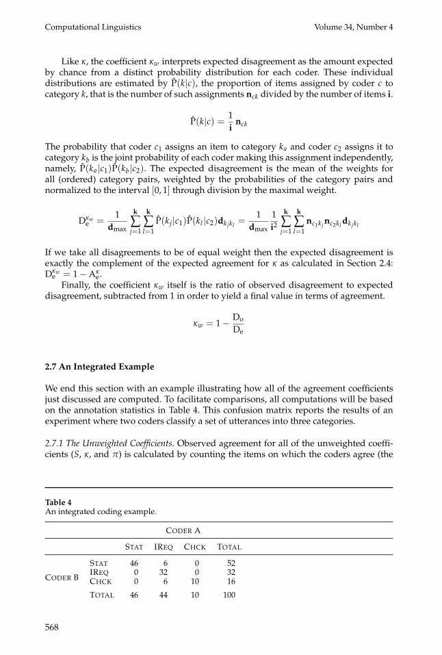
2.7 An Integrated Example
We end this section with an example illustrating how all of the agreement coefficientsjust discussed are computed. To facilitate comparisons, all computations will be basedon the annotation statistics in Table 4. This confusion matrix reports the results of anexperiment where two coders classify a set of utterances into three categories.
2.7.1 The Unweighted Coefficients. Observed agreement for all of the unweighted coeffi-cients (S, κ, and π) is calculated by counting the items on which the coders agree (the
Table 4An integrated coding example.
CODER A
STAT IREQ CHCK TOTAL
STAT 46 6 0 52IREQ 0 32 0 32
CODER B CHCK 0 6 10 16
TOTAL 46 44 10 100
568

Artstein and Poesio Inter-Coder Agreement for CL
figures on the diagonal of the confusion matrix in Table 4) and dividing by the totalnumber of items.
Ao =46+ 32+ 10
100= 0.88
The expected agreement values and the resulting values for the coefficients are shown inTable 5. The values of π and κ are very similar, which is to be expected when agreementis high, because this implies similar marginals. Notice that Aκ
e < Aπe , hence κ > π; this
reflects a general property of κ and π, already mentioned in Section 2.4, which will beelaborated in Section 3.1.
2.7.2 Weighted Coefficients. Suppose we notice that whereas Statement and Info-Request are clearly distinct classifications, Check is somewhere between the two. Wetherefore opt to weigh the distances between the categories as follows (recall that1 denotes maximal disagreement, and identical categories are in full agreement andthus have a distance of 0).
Statement Info-Request CheckStatement 0 1 0.5Info-Request 1 0 0.5Check 0.5 0.5 0
The observed disagreement is calculated by summing up all the cells in the contingencytable, multiplying each cell by its respective weight, and dividing the total by thenumber of items (in the following calculation we ignore cells with zero items).
Do =46× 0+ 6× 1+ 32× 0+ 6× 0.5+ 10× 0
100=
6+ 3100
= 0.09
The only sources of disagreement in the coding example of Table 4 are the six utterancesmarked as Info-Requests by coder A and Statements by coder B, which receive themaximal weight of 1, and the six utterances marked as Info-Requests by coder A andChecks by coder B, which are given a weight of 0.5.
The calculation of expected disagreement for the weighted coefficients is shown inTable 6, and is the sum of the expected disagreement for each category pair multiplied
Table 5Unweighted coefficients for the data from Table 4.
Expected agreement Chance-corrected agreement
S 3× ( 13 )2 = 1
3 (0.88− 13 )/(1− 1
3 ) = 0.82
π 0.46+0.522 + 0.44+0.32
2 + 0.10+0.162 = 0.4014 (0.88− 0.4014)/(1− 0.4014) ≈ 0.7995
κ .46× .52+ .44× .32+ .1× .16 = 0.396 (0.88− 0.396)/(1− 0.396) ≈ 0.8013
569

Computational Linguistics Volume 34, Number 4
Table 6Expected disagreement of the weighted coefficients for the data from Table 4.
Dαe
(46+52)×(46+52)2×100×(2×100−1) × 0+ (44+32)×(46+52)
2×100×(2×100−1) × 1 + (10+16)×(46+52)2×100×(2×100−1) ×
12
+ (46+52)×(44+32)2×100×(2×100−1) × 1 + (44+32)×(44+32)
2×100×(2×100−1) × 0 + (10+16)×(44+32)2×100×(2×100−1) ×
12
+ (46+52)×(10+16)2×100×(2×100−1) ×
12 + (44+32)×(10+16)
2×100×(2×100−1) ×12 + (10+16)×(10+16)
2×100×(2×100−1) × 0
0.4879
Dκwe
46×52100×100 × 0+ 44×52
100×100 × 1 + 10×52100×100 ×
12
+ 46×32100×100 × 1 + 44×32
100×100 × 0 + 10×32100×100 ×
12
+ 46×16100×100 ×
12 + 44×16
100×100 ×12 + 10×16
100×100 × 0
0.49
by its weight. The value of the weighted coefficients is given by the formula 1− DoDe, so
α ≈ 1− 0.090.4879 ≈ 0.8156, and κw = 1− 0.09
0.49 ≈ 0.8163.
3. Bias and Prevalence
Two issues recently raised by Di Eugenio and Glass (2004) concern the behavior ofagreement coefficients when the annotation data are severely skewed. One issue, whichDi Eugenio and Glass call the bias problem, is that π and κ yield quite differentnumerical values when the annotators’ marginal distributions are widely divergent;the other issue, the prevalence problem, is the exceeding difficulty in getting highagreement values when most of the items fall under one category. Looking at these twoproblems in detail is useful for understanding the differences between the coefficients.
3.1 Annotator Bias
The difference between π and α on the one hand and κ on the other hand lies in theinterpretation of the notion of chance agreement, whether it is the amount expectedfrom the the actual distribution of items among categories (π) or from individual coderpriors (κ). As mentioned in Section 2.4, this difference has been the subject of muchdebate (Fleiss 1975; Krippendorff 1978, 2004b; Byrt, Bishop, andCarlin 1993; Zwick 1988;Hsu and Field 2003; Di Eugenio and Glass 2004; Craggs and McGee Wood 2005).
A claim often repeated in the literature is that single-distribution coefficients likeπ and α assume that different coders produce similar distributions of items amongcategories, with the implication that these coefficients are inapplicable when the anno-tators show substantially different distributions. Recommendations vary: Zwick (1988)suggests testing the individual coders’ distributions using the modified χ2 test of Stuart(1955), and discarding the annotation as unreliable if significant systematic discrepan-cies are observed. In contrast, Hsu and Field (2003, page 214) recommend reportingthe value of κ even when the coders produce different distributions, because it is “theonly [index] . . . that could legitimately be applied in the presence of marginal hetero-geneity”; likewise, Di Eugenio andGlass (2004, page 96) recommend using κ in “the vastmajority . . . of discourse- and dialogue-tagging efforts” where the individual coders’distributions tend to vary. All of these proposals are based on a misconception: that
570

Artstein and Poesio Inter-Coder Agreement for CL
single-distribution coefficients require similar distributions by the individual annota-tors in order to work properly. This is not the case. The difference between the coeffi-cients is only in the interpretation of “chance agreement”: π-style coefficients calculatethe chance of agreement among arbitrary coders, whereas κ-style coefficients calcu-late the chance of agreement among the coders who produced the reliability data. There-fore, the choice of coefficient should not depend on the magnitude of the divergencebetween the coders, but rather on the desired interpretation of chance agreement.
Another common claim is that individual-distribution coefficients like κ “reward”annotators for disagreeing on the marginal distributions. For example, Di Eugenio andGlass (2004, page 99) say that κ suffers from what they call the bias problem, describedas “the paradox that κCo [our κ] increases as the coders become less similar.” Similarreservations about the use of κ have been noted by Brennan and Prediger (1981) andZwick (1988). However, the bias problem is less paradoxical than it sounds. Althoughit is true that for a fixed observed agreement, a higher difference in coder marginalsimplies a lower expected agreement and therefore a higher κ value, the conclusion thatκ penalizes coders for having similar distributions is unwarranted. This is because Aoand Ae are not independent: Both are drawn from the same set of observations. Whatκ does is discount some of the disagreement resulting from different coder marginals byincorporating it into Ae. Whether this is desirable depends on the application for whichthe coefficient is used.
Themost common application of agreement measures in CL is to infer the reliabilityof a large-scale annotation, where typically each piece of data will be marked by justone coder, by measuring agreement on a small subset of the data which is annotatedby multiple coders. In order to make this generalization, the measure must reflect thereliability of the annotation procedure, which is independent of the actual annotatorsused. Reliability, or reproducibility of the coding, is reduced by all disagreements—bothrandom and systematic. The most appropriate measures of reliability for this purposeare therefore single-distribution coefficients like π and α, which generalize over theindividual coders and exclude marginal disagreements from the expected agreement.This argument has been presented recently in much detail by Krippendorff (2004b) andreiterated by Craggs and McGee Wood (2005).
At the same time, individual-distribution coefficients like κ provide important in-formation regarding the trustworthiness (validity) of the data on which the annotatorsagree. As an intuitive example, think of a person who consults two analysts whendeciding whether to buy or sell certain stocks. If one analyst is an optimist and tends torecommend buying whereas the other is a pessimist and tends to recommend selling,they are likely to agree with each other less than two more neutral analysts, so overalltheir recommendations are likely to be less reliable—less reproducible—than those thatcome from a population of like-minded analysts. This reproducibility is measured by π.But whenever the optimistic and pessimistic analysts agree on a recommendation fora particular stock, whether it is “buy” or “sell,” the confidence that this is indeed theright decision is higher than the same advice from two like-minded analysts. This iswhy κ “rewards” biased annotators: it is not a matter of reproducibility (reliability) butrather of trustworthiness (validity).
Having said this, we should point out that, first, in practice the difference betweenπ and κ doesn’t often amount to much (see discussion in Section 4). Moreover, thedifference becomes smaller as agreement increases, because all the points of agreementcontribute toward making the coder marginals similar (it took a lot of experimentationto create data for Table 4 so that the values of π and κ would straddle the conventionalcutoff point of 0.80, and even so the difference is very small). Finally, one would expect
571

Computational Linguistics Volume 34, Number 4
the difference between π and κ to diminish as the number of coders grows; this is shownsubsequently.6
We define B, the overall annotator bias in a particular set of coding data, as thedifference between the expected agreement according to (multi)-π and the expectedagreement according to (multi)-κ. Annotator bias is a measure of variance: If we take c tobe a random variable with equal probabilities for all coders, then the annotator bias Bis the sum of the variances of P(k|c) for all categories k ∈ K, divided by the number ofcoders c less one (see Artstein and Poesio [2005] for a proof).
B = Aπe −Aκ
e =1
c− 1 ∑k∈K
σ2P(k|c)
Annotator bias can be used to express the difference between κ and π.
κ − π =Ao − (Aπ
e − B)1− (Aπ
e − B)−Ao −Aπ
e
1−Aπe
= B ·(1−Ao)
(1−Aκe)(1−Aπ
e )
This allows us to make the following observations about the relationship betweenπ and κ.
Observation 1. The difference between κ and π grows as the annotator bias grows: For aconstant Ao and Aπ
e , a greater B implies a greater value for κ − π.
Observation 2. The greater the number of coders, the lower the annotator bias B, and hencethe lower the difference between κ and π, because the variance of P(k|c) does not increase inproportion to the number of coders.
In other words, provided enough coders are used, it should not matter whether asingle-distribution or individual-distribution coefficient is used. This is not to imply thatmultiple coders increase reliability: The variance of the individual coders’ distributionscan be just as large with many coders as with few coders, but its effect on the valueof κ decreases as the number of coders grows, and becomes more similar to randomnoise.
The same holds for weighted measures too; see the extended version of this articlefor definitions and proof. In an annotation study with 18 subjects, we compared α witha variant which uses individual coder distributions to calculate expected agreement,and found that the values never differed beyond the third decimal point (Poesio andArtstein 2005).
We conclude with a summary of our views concerning the difference between π-style and κ-style coefficients. First of all, keep in mind that empirically the differenceis small, and gets smaller as the number of annotators increases. Then instead ofreporting two coefficients, as suggested by Di Eugenio and Glass (2004), the appropriatecoefficient should be chosen based on the task (not on the observed differences betweencoder marginals). When the coefficient is used to assess reliability, a single-distributioncoefficient like π or α should be used; this is indeed already the practice in CL, becauseSiegel and Castellan’s K is identical with (multi-)π. It is also good practice to test
6 Craggs and McGee Wood (2005) also suggest increasing the number of coders in order to overcomeindividual annotator bias, but do not provide a mathematical justification.
572

Artstein and Poesio Inter-Coder Agreement for CL
reliability withmore than two coders, in order to reduce the likelihood of coders sharinga deviant reading of the annotation guidelines.
3.2 Prevalence
We touched upon the matter of skewed data in Section 2.3 when we motivated the needfor chance correction: If a disproportionate amount of the data falls under one category,then the expected agreement is very high, so in order to demonstrate high reliabilityan even higher observed agreement is needed. This leads to the so-called paradox thatchance-corrected agreement may be low even though Ao is high (Cicchetti and Feinstein1990; Feinstein and Cicchetti 1990; Di Eugenio and Glass 2004). Moreover, when thedata are highly skewed in favor of one category, the high agreement also correspondsto high accuracy: If, say, 95% of the data fall under one category label, then randomcoding would cause two coders to jointly assign this category label to 90.25% of theitems, and on average 95% of these labels would be correct, for an overall accuracy of atleast 85.7%. This leads to the surprising result that when data are highly skewed, codersmay agree on a high proportion of items while producing annotations that are indeedcorrect to a high degree, yet the reliability coefficients remain low. (For an illustration,see the discussion of agreement results on coding discourse segments in Section 4.3.1.)
This surprising result is, however, justified. Reliability implies the ability to dis-tinguish between categories, but when one category is very common, high accuracyand high agreement can also result from indiscriminate coding. The test for reliabil-ity in such cases is the ability to agree on the rare categories (regardless of whetherthese are the categories of interest). Indeed, chance-corrected coefficients are sensitiveto agreement on rare categories. This is easiest to see with a simple example of twocoders and two categories, one common and the other one rare; to further simplify thecalculation we also assume that the coder marginals are identical, so that π and κ yieldthe same values. We can thus represent the judgments in a contingency table with justtwo parameters: ε is half the proportion of items on which there is disagreement, andδ is the proportion of agreement on the Rare category. Both of these proportions areassumed to be small, so the bulk of the items (a proportion of 1− (δ + 2ε)) are labeledwith the Common category by both coders (Table 7). From this table we can calculateAo = 1− 2ε and Ae = 1− 2(δ + ε) + 2(δ + ε)2, as well as π and κ.
π, κ =1− 2ε − (1− 2(δ + ε) + 2(δ + ε)2)1− (1− 2(δ + ε) + 2(δ + ε)2)
=δ
δ + ε−
ε
1− (δ + ε)
When ε and δ are both small, the fraction after the minus sign is small as well, so π and κare approximately δ/(δ + ε): the value we get if we take all the items marked by one
Table 7A simple example of agreement on dialogue act tagging.
CODER A
COMMON RARE TOTAL
COMMON 1− (δ + 2ε) ε 1− (δ + ε)
CODER B RARE ε δ δ + εTOTAL 1− (δ + ε) δ + ε 1
573

Computational Linguistics Volume 34, Number 4
particular coder asRare, and calculate what proportion of those itemswere labeledRareby the other coder. This is a measure of the coders’ ability to agree on the rare category.
4. Using Agreement Measures for CL Annotation Tasks
In this section we review the use of intercoder agreement measures in CL sinceCarletta’s original paper in light of the discussion in the previous sections. We beginwith a summary of Krippendorff’s recommendations about measuring reliability(Krippendorff 2004a, Chapter 11), then discuss how coefficients of agreement havebeen used in CL to measure the reliability of annotation schemes, focusing in particularon the types of annotation where there has been some debate concerning the mostappropriate measures of agreement.
4.1 Methodology and Interpretation of the Results: General Issues
Krippendorff (2004a, Chapter 11) notes with regret the fact that reliability is discussed inonly around 69% of studies in content analysis. In CL as well, not all annotation projectsinclude a formal test of intercoder agreement. Some of the best known annotationefforts, such as the creation of the Penn Treebank (Marcus, Marcinkiewicz, and Santorini1993) and the British National Corpus (Leech, Garside, and Bryant 1994), do not reportreliability results as they predate the Carletta paper; but even among the more recentefforts, many only report percentage agreement, as for the creation of the PropBank(Palmer, Dang, and Fellbaum 2007) or the ongoing OntoNotes annotation (Hovy et al.2006). Even more importantly, very few studies apply a methodology as rigorous asthat envisaged by Krippendorff and other content analysts. We therefore begin thisdiscussion of CL practice with a summary of the main recommendations found inChapter 11 of Krippendorff (2004a), even though, as we will see, we think that someof these recommendations may not be appropriate for CL.
4.1.1 Generating Data to Measure Reproducibility. Krippendorff’s recommendations weredeveloped for the field of content analysis, where coding is used to draw conclusionsfrom the texts. A coded corpus is thus akin to the result of a scientific experiment, andit can only be considered valid if it is reproducible—that is, if the same coded resultscan be replicated in an independent coding exercise. Krippendorff therefore argues thatany study using observed agreement as a measure of reproducibility must satisfy thefollowing requirements:
• It must employ an exhaustively formulated, clear, and usable codingscheme together with step-by-step instructions on how to use it.
• It must use clearly specified criteria concerning the choice of coders(so that others may use such criteria to reproduce the data).
• It must ensure that the coders that generate the data used to measurereproducibility work independently of each other.
Some practices that are common in CL do not satisfy these requirements. The firstrequirement is violated by the practice of expanding the written coding instructionsand including new rules as the data are generated. The second requirement is often
574

Artstein and Poesio Inter-Coder Agreement for CL
violated by using experts as coders, particularly long-term collaborators, as such codersmay agree not because they are carefully following written instructions, but becausethey know the purpose of the research very well—which makes it virtually impossiblefor others to reproduce the results on the basis of the same coding scheme (the prob-lems arising when using experts were already discussed at length in Carletta [1996]).Practices which violate the third requirement (independence) include asking coders todiscuss their judgments with each other and reach their decisions by majority vote, orto consult with each other when problems not foreseen in the coding instructions arise.Any of these practices make the resulting data unusable for measuring reproducibility.
Krippendorff’s own summary of his recommendations is that to obtain usabledata for measuring reproducibility a researcher must use data generated by three ormore coders, chosen according to some clearly specified criteria, and working indepen-dently according to a written coding scheme and coding instructions fixed in advance.Krippendorff also discusses the criteria to be used in the selection of the sample, fromthe minimum number of units (obtained using a formula from Bloch and Kraemer[1989], reported in Krippendorff [2004a, page 239]), to how to make the sample rep-resentative of the data population (each category should occur in the sample oftenenough to yield at least five chance agreements), to how to ensure the reliability of theinstructions (the sample should contain examples of all the values for the categories).These recommendations are particularly relevant in light of the comments of Craggsand McGee Wood (2005, page 290), which discourage researchers from testing theircoding instructions on data from more than one domain. Given that the reliability ofthe coding instructions depends to a great extent on how complications are dealt with,and that every domain displays different complications, the sample should containsufficient examples from all domains which have to be annotated according to theinstructions.
4.1.2 Establishing Significance. In hypothesis testing, it is common to test for the sig-nificance of a result against a null hypothesis of chance behavior; for an agreementcoefficient this would mean rejecting the possibility that a positive value of agreementis nevertheless due to random coding. We can rely on the statement by Siegel andCastellan (1988, Section 9.8.2) that when sample sizes are large, the sampling distribu-tion of K (Fleiss’s multi-π) is approximately normal and centered around zero—thisallows testing the obtained value of K against the null hypothesis of chance agreementby using the z statistic. It is also easy to test Krippendorff’s α with the interval distancemetric against the null hypothesis of chance agreement, because the hypothesis α = 0 isidentical to the hypothesis F = 1 in an analysis of variance.
However, a null hypothesis of chance agreement is not very interesting, and demon-strating that agreement is significantly better than chance is not enough to establishreliability. This has already been pointed out by Cohen (1960, page 44): “to knowmerelythat κ is beyond chance is trivial since one usually expects much more than this in theway of reliability in psychological measurement.” The same point has been repeatedand stressed in many subsequent works (e.g., Posner et al. 1990; Di Eugenio 2000;Krippendorff 2004a): The reason for measuring reliability is not to test whether codersperform better than chance, but to ensure that the coders do not deviate too much fromperfect agreement (Krippendorff 2004a, page 237).
The relevant notion of significance for agreement coefficients is therefore a confi-dence interval. Cohen (1960, pages 43–44) implies that when sample sizes are large,the sampling distribution of κ is approximately normal for any true population valueof κ, and therefore confidence intervals for the observed value of κ can be determined
575

Computational Linguistics Volume 34, Number 4
using the usual multiples of the standard error. Donner and Eliasziw (1987) proposea more general form of significance test for arbitrary levels of agreement. In contrast,Krippendorff (2004a, Section 11.4.2) states that the distribution of α is unknown, soconfidence intervals must be obtained by bootstrapping; a software package for doingthis is described in Hayes and Krippendorff (2007).
4.1.3 Interpreting the Value of Kappa-Like Coefficients. Even after testing significance andestablishing confidence intervals for agreement coefficients, we are still faced with theproblem of interpreting the meaning of the resulting values. Suppose, for example, weestablish that for a particular task, K = 0.78± 0.05. Is this good or bad? Unfortunately,deciding what counts as an adequate level of agreement for a specific purpose is stilllittle more than a black art: As we will see, different levels of agreement may beappropriate for resource building and for more linguistic purposes.
The problem is not unlike that of interpreting the values of correlation coefficients,and in the area of medical diagnosis, the best known conventions concerning the valueof kappa-like coefficients, those proposed by Landis and Koch (1977) and reported inFigure 1, are indeed similar to those used for correlation coefficients, where valuesabove 0.4 are also generally considered adequate (Marion 2004). Many medical re-searchers feel that these conventions are appropriate, and in language studies, a similarinterpretation of the values has been proposed by Rietveld and van Hout (1993). InCL, however, most researchers follow the more stringent conventions from contentanalysis proposed by Krippendorff (1980, page 147), as reported by Carletta (1996,page 252): “content analysis researchers generally think of K > .8 as good reliability,with .67 < K < .8 allowing tentative conclusions to be drawn” (Krippendorff was dis-cussing values of α rather than K, but the coefficients are nearly equivalent for cate-gorical labels). As a result, ever since Carletta’s influential paper, CL researchers haveattempted to achieve a value of K (more seldom, of α) above the 0.8 threshold, or, failingthat, the 0.67 level allowing for “tentative conclusions.” However, the description ofthe 0.67 boundary in Krippendorff (1980) was actually “highly tentative and cautious,”and in later work Krippendorff clearly considers 0.8 the absolute minimum value ofα to accept for any serious purpose: “Even a cutoff point of α = .800 . . . is a prettylow standard” (Krippendorff 2004a, page 242). Recent content analysis practice seemsto have settled for even more stringent requirements: A recent textbook, Neuendorf(2002, page 3), analyzing several proposals concerning “acceptable” reliability, con-cludes that “reliability coefficients of .90 or greater would be acceptable to all, .80or greater would be acceptable in most situations, and below that, there exists greatdisagreement.”
This is clearly a fundamental issue. Ideally we would want to establish thresholdswhich are appropriate for the field of CL, but as we will see in the rest of this section, adecade of practical experience hasn’t helped in settling the matter. In fact, weightedcoefficients, while arguably more appropriate for many annotation tasks, make theissue of deciding when the value of a coefficient indicates sufficient agreement even
K = 0.0 0.2 0.4 0.6 0.8 1.0
Poor Slight Fair Moderate Substantial Perfect
Figure 1Kappa values and strength of agreement according to Landis and Koch (1977).
576

Artstein and Poesio Inter-Coder Agreement for CL
more complicated because of the problem of determining appropriate weights (seeSection 4.4). We will return to the issue of interpreting the value of the coefficients atthe end of this article.
4.1.4 Agreement and Machine Learning. In a recent article, Reidsma and Carletta (2008)point out that the goals of annotation in CL differ from those of content analysis, whereagreement coefficients originate. A common use of an annotated corpus in CL is notto confirm or reject a hypothesis, but to generalize the patterns using machine-learningalgorithms. Through a series of simulations, Reidsma and Carletta demonstrate thatagreement coefficients are poor predictors of machine-learning success: Even highlyreproducible annotations are difficult to generalize when the disagreements contain pat-terns that can be learned, whereas highly noisy and unreliable data can be generalizedsuccessfully when the disagreements do not contain learnable patterns. These resultsshow that agreement coefficients should not be used as indicators of the suitability ofannotated data for machine learning.
However, the purpose of reliability studies is not to find out whether annotationscan be generalized, but whether they capture some kind of observable reality. Even ifthe pattern of disagreement allows generalization, we need evidence that this general-ization would be meaningful. The decision whether a set of annotation guidelines areappropriate or meaningful is ultimately a qualitative one, but a baseline requirement isan acceptable level of agreement among the annotators, who serve as the instrumentsof measurement. Reliability studies test the soundness of an annotation scheme andguidelines, which is not to be equated with the machine-learnability of data producedby such guidelines.
4.2 Labeling Units with a Common and Predefined Set of Categories: The Caseof Dialogue Act Tagging
The simplest and most common coding in CL involves labeling segments of text witha limited number of linguistic categories: Examples include part-of-speech tagging,dialogue act tagging, and named entity tagging. The practices used to test reliabilityfor this type of annotation tend to be based on the assumption that the categories usedin the annotation are mutually exclusive and equally distinct from one another; thisassumption seems to have worked out well in practice, but questions about it have beenraised even for the annotation of parts of speech (Babarczy, Carroll, and Sampson 2006),let alone for discourse coding tasks such as dialogue act coding. We concentrate here onthis latter type of coding, but a discussion of issues raised for POS, named entity, andprosodic coding can be found in the extended version of the article.
Dialogue act tagging is a type of linguistic annotation with which by now the CLcommunity has had extensive experience: Several dialogue-act-annotated spoken lan-guage corpora now exist, such as MapTask (Carletta et al. 1997), Switchboard (Stolckeet al. 2000), Verbmobil (Jekat et al. 1995), and Communicator (e.g., Doran et al. 2001),among others. Historically, dialogue act annotation was also one of the types of annota-tion that motivated the introduction in CL of chance-corrected coefficients of agreement(Carletta et al. 1997) and, as we will see, it has been the type of annotation that hasgenerated the most discussion concerning annotation methodology and measuringagreement.
A number of coding schemes for dialogue acts have achieved values of K over0.8 and have therefore been assumed to be reliable: For example, K = 0.83 for the
577

Computational Linguistics Volume 34, Number 4
13-tagMapTask coding scheme (Carletta et al. 1997), K = 0.8 for the 42-tag Switchboard-DAMSL scheme (Stolcke et al. 2000), K = 0.90 for the smaller 20-tag subset of the CSTARscheme used by Doran et al. (2001). All of these tests were based on the same twoassumptions: that every unit (utterance) is assigned to exactly one category (dialogueact), and that these categories are distinct. Therefore, again, unweighted measures, andin particular K, tend to be used for measuring inter-coder agreement.
However, these assumptions have been challenged based on the observation thatutterances tend to have more than one function at the dialogue act level (Traum andHinkelman 1992; Allen and Core 1997; Bunt 2000); for a useful survey, see Popescu-Belis(2005). An assertion performed in answer to a question, for instance, typically performsat least two functions at different levels: asserting some information—the dialogue actthat we called Statement in Section 2.3, operating at what Traum and Hinkelman calledthe “core speech act” level—and confirming that the question has been understood, a di-alogue act operating at the “grounding” level and usually known as Acknowledgment(Ack). In older dialogue act tagsets, acknowledgments and statements were treated asalternative labels at the same “level”, forcing coders to choose one or the other when anutterance performed a dual function, according to a well-specified set of instructions. Bycontrast, in the annotation schemes inspired from these newer theories such as DAMSL(Allen and Core 1997), coders are allowed to assign tags along distinct “dimensions” or“levels”.
Two annotation experiments testing this solution to the “multi-tag” problem withthe DAMSL scheme were reported in Core and Allen (1997) and Di Eugenio et al.(1998). In both studies, coders were allowed to mark each communicative functionindependently: That is, they were allowed to choose for each utterance one of theStatement tags (or possibly none), one of the Influencing-Addressee-Future-Actiontags, and so forth—and agreement was evaluated separately for each dimension using(unweighted) K. Core and Allen found values of K ranging from 0.76 for answerto 0.42 for agreement to 0.15 for Committing-Speaker-Future-Action. Using differ-ent coding instructions and on a different corpus, Di Eugenio et al. observed higheragreement, ranging from K = 0.93 (for other-forward-function) to 0.54 (for the tagagreement).
These relatively low levels of agreement led many researchers to return to “flat”tagsets for dialogue acts, incorporating however in their schemes some of the in-sights motivating the work on schemes such as DAMSL. The best known exampleof this type of approach is the development of the SWITCHBOARD-DAMSL tagsetby Jurafsky, Shriberg, and Biasca (1997), which incorporates many ideas from the“multi-dimensional” theories of dialogue acts, but does not allow marking an utteranceas both an acknowledgment and a statement; a choice has to be made. This tagsetresults in overall agreement of K = 0.80. Interestingly, subsequent developments ofSWITCHBOARD-DAMSL backtracked on some of these decisions. For instance, theICSI-MRDA tagset developed for the annotation of the ICSI Meeting Recorder corpusreintroduces some of the DAMSL ideas, in that annotators are allowed to assign multi-ple SWITCHBOARD-DAMSL labels to utterances (Shriberg et al. 2004). Shriberg et al.achieved a comparable reliability to that obtained with SWITCHBOARD-DAMSL, butonly when using a tagset of just five “class-maps”.
Shriberg et al. (2004) also introduced a hierarchical organization of tags to improvereliability. The dimensions of the DAMSL scheme can be viewed as “superclasses” ofdialogue acts which share some aspect of their meaning. For instance, the dimensionof Influencing-Addressee-Future-Action (IAFA) includes the two dialogue actsOpen-option (used to mark suggestions) and Directive, both of which bring into
578

Artstein and Poesio Inter-Coder Agreement for CL
consideration a future action to be performed by the addressee. At least in principle,an organization of this type opens up the possibility for coders to mark an utterancewith the superclass (IAFA) in case they do not feel confident that the utterance satisfiesthe additional requirements for Open-option or Directive. This, in turn, would doaway with the need to make a choice between these two options. This possibilitywasn’t pursued in the studies using the original DAMSL that we are aware of (Coreand Allen 1997; Di Eugenio 2000; Stent 2001), but was tested by Shriberg et al. (2004)and subsequent work, in particular Geertzen and Bunt (2006), who were specificallyinterested in the idea of using hierarchical schemes to measure partial agreement, andin addition experimented with weighted coefficients of agreement for their hierarchicaltagging scheme, specifically κw.
Geertzen and Bunt tested intercoder agreement with Bunt’s DIT++ (Bunt 2005),a scheme with 11 dimensions that builds on ideas from DAMSL and from DynamicInterpretation Theory (Bunt 2000). In DIT++, tags can be hierarchically related: Forexample, the class information-seeking is viewed as consisting of two classes, yes-no question (ynq) and wh-question (whq). The hierarchy is explicitly introduced in orderto allow coders to leave some aspects of the coding undecided. For example, check istreated as a subclass of ynq in which, in addition, the speaker has a weak belief that theproposition that forms the belief is true. A coder who is not certain about the dialogueact performed using an utterance may simply choose to tag it as ynq.
The distance metric d proposed by Geertzen and Bunt is based on the crite-rion that two communicative functions are related (d(c1, c2) < 1) if they stand in anancestor–offspring relation within a hierarchy. Furthermore, they argue, the magnitudeof d(c1, c2) should be proportional to the distance between the functions in the hierar-chy. A level-dependent correction factor is also proposed so as to leave open the optiontomake disagreements at higher levels of the hierarchymatter more than disagreementsat the deeper level (for example, the distance between information-seeking and ynqmight be considered greater than the distance between check and positive-check).
The results of an agreement test with two annotators run by Geertzen and Buntshow that taking into account partial agreement leads to values of κw that are higherthan the values of κ for the same categories, particularly for feedback, a class for whichCore andAllen (1997) got low agreement. Of course, even assuming that the values of κwand κ were directly comparable—we remark on the difficulty of interpreting the valuesof weighted coefficients of agreement in Section 4.4—it remains to be seenwhether thesehigher values are a better indication of the extent of agreement between coders than thevalues of unweighted κ.
This discussion of coding schemes for dialogue acts introduced issues to whichwe will return for other CL annotation tasks as well. There are a number of well-established schemes for large-scale dialogue act annotation based on the assumptionof mutual exclusivity between dialogue act tags, whose reliability is also well known; ifone of these schemes is appropriate for modeling the communicative intentions foundin a task, we recommend to our readers to use it. They should also realize, however,that the mutual exclusivity assumption is somewhat dubious. If a multi-dimensional orhierarchical tagset is used, readers should also be aware that weighted coefficients docapture partial agreement, and need not automatically result in lower reliability or inan explosion in the number of labels. However, a hierarchical scheme may not reflectgenuine annotation difficulties: For example, in the case of DIT++, one might argue thatit is more difficult to confuse yes-no questions with wh-questions than with statements.We will also see in a moment that interpreting the results with weighted coefficients isdifficult. We will return to both of these problems in what follows.
579

Computational Linguistics Volume 34, Number 4
4.3 Marking Boundaries and Unitizing
Before labeling can take place, the units of annotation, or markables, need to beidentified—a process Krippendorff (1995, 2004a) calls unitizing. The practice in CL forthe forms of annotation discussed in the previous section is to assume that the units arelinguistic constituents which can be easily identified, such as words, utterances, or nounphrases, and therefore there is no need to check the reliability of this process. We areaware of few exceptions to this assumption, such as Carletta et al. (1997) on unitizationfor move coding and our own work on the GNOME corpus (Poesio 2004b). In casessuch as text segmentation, however, the identification of units is as important as theirlabeling, if not more important, and therefore checking agreement on unit identificationis essential. In this section we discuss current CL practice with reliability testing of thesetypes of annotation, before briefly summarizing Krippendorff’s proposals concerningmeasuring reliability for unitizing.
4.3.1 Segmentation and Topic Marking. Discourse segments are portions of text that con-stitute a unit either because they are about the same “topic” (Hearst 1997; Reynar1998) or because they have to do with achieving the same intention (Grosz and Sidner1986) or performing the same “dialogue game” (Carletta et al. 1997).7 The analysisof discourse structure—and especially the identification of discourse segments—is thetype of annotation that, more than any other, led CL researchers to look for ways ofmeasuring reliability and agreement, as it made them aware of the extent of disagree-ment on even quite simple judgments (Kowtko, Isard, and Doherty 1992; Passonneauand Litman 1993; Carletta et al. 1997; Hearst 1997). Subsequent research identified anumber of issues with discourse structure annotation, above all the fact that segmen-tation, though problematic, is still much easier than marking more complex aspects ofdiscourse structure, such as identifying the most important segments or the “rhetorical”relations between segments of different granularity. As a result, many efforts to annotatediscourse structure concentrate only on segmentation.
The agreement results for segment coding tend to be on the lower end of thescale proposed by Krippendorff and recommended by Carletta. Hearst (1997), forinstance, found K = 0.647 for the boundary/not boundary distinction; Reynar (1998),measuring agreement between his own annotation and the TREC segmentation ofbroadcast news, reports K = 0.764 for the same task; Ries (2002) reports even loweragreement of K = 0.36. Teufel, Carletta, and Moens (1999), who studied agreement onthe identification of argumentative zones, found high reliability (K = 0.81) for theirthree main zones (own, other, background), although lower for the whole scheme(K = 0.71). For intention-based segmentation, Passonneau and Litman (1993) in thepre-K days reported an overall percentage agreement with majority opinion of 89%, butthe agreement on boundaries was only 70%. For conversational games segmentation,Carletta et al. (1997) reported “promising but not entirely reassuring agreement onwhere games began (70%),” whereas the agreement on transaction boundaries wasK = 0.59. Exceptions are two segmentation efforts carried out as part of annotationsof rhetorical structure. Moser, Moore, and Glendening (1996) achieved an agreement
7 The notion of “topic” is notoriously difficult to define and many competing theoretical proposals exist(Reinhart 1981; Vallduvı 1993). As it is often the case with annotation, fairly simple definitions tend tobe used in discourse annotation work: For example, in TDT topic is defined for annotation purposesas “an event or activity, along with all directly related events and activities” (TDT-2 Annotation Guide,http://projects.ldc.upenn.edu/TDT2/Guide/label-instr.html).
580

Artstein and Poesio Inter-Coder Agreement for CL
of K = 0.9 for the highest level of segmentation of their RDA annotation (Poesio,Patel, and Di Eugenio 2006). Carlson, Marcu, and Okurowski (2003) reported veryhigh agreement over the identification of the boundaries of discourse units, the build-ing blocks of their annotation of rhetorical structure. (Agreement was measured sev-eral times; initially, they obtained K = 0.87, and in the final analysis K = 0.97.) This,however, was achieved by employing experienced annotators, and with considerabletraining.
One important reason why most agreement results on segmentation are on thelower end of the reliability scale is the fact, known to researchers in discourse analysisfrom as early as Levin and Moore (1978), that although analysts generally agree on the“bulk” of segments, they tend to disagree on their exact boundaries. This phenomenonwas also observed in more recent studies: See for example the discussion in Passonneauand Litman (1997), the comparison of the annotations produced by seven coders ofthe same text in Figure 5 of Hearst (1997, page 55), or the discussion by Carlson,Marcu, and Okurowski (2003), who point out that the boundaries between elementarydiscourse units tend to be “very blurry.” See also Pevzner and Hearst (2002) for similarcomments made in the context of topic segmentation algorithms, and Klavans, Popper,and Passonneau (2003) for selecting definition phrases.
This “blurriness” of boundaries, combined with the prevalence effects discussedin Section 3.2, also explains the fact that topic annotation efforts which were onlyconcerned with roughly dividing a text into segments (Passonneau and Litman 1993;Carletta et al. 1997; Hearst 1997; Reynar 1998; Ries 2002) generally report lower agree-ment than the studies whose goal is to identify smaller discourse units. When disagree-ment is mostly concentrated in one class (‘boundary’ in this case), if the total number ofunits to annotate remains the same, then expected agreement on this class is lower whena greater proportion of the units to annotate belongs to this class. When in addition thisclass is much less numerous than the other classes, overall agreement tends to dependmostly on agreement on this class.
For instance, suppose we are testing the reliability of two different segmentationschemes—into broad “discourse segments” and into finer “discourse units”—on a textof 50 utterances, and that we obtain the results in Table 8. Case 1 would be a situationin which Coder A and Coder B agree that the text consists of two segments, obviouslyagree on its initial and final boundaries, but disagree by one position on the intermediateboundary—say, one of them places it at utterance 25, the other at utterance 26. Never-theless, because expected agreement is so high—the coders agree on the classificationof 98% of the utterances—the value of K is fairly low. In case 2, the coders disagree onthree times as many utterances, but K is higher than in the first case because expectedagreement is substantially lower (Ae = 0.53).
The fact that coders mostly agree on the “bulk” of discourse segments, but tendto disagree on their boundaries, also makes it likely that an all-or-nothing coefficientlike K calculated on individual boundaries would underestimate the degree of agree-ment, suggesting low agreement even among coders whose segmentations are mostlysimilar. A weighted coefficient of agreement like α might produce values more inkeeping with intuition, but we are not aware of any attempts at measuring agreementon segmentation using weighted coefficients. We see two main options. We suspect thatthe methods proposed by Krippendorff (1995) for measuring agreement on unitizing(see Section 4.3.2, subsequently) may be appropriate for the purpose of measuringagreement on discourse segmentation. A second optionwould be tomeasure agreementnot on individual boundaries but on windows spanning several units, as done in themethods proposed to evaluate the performance of topic detection algorithms such as
581
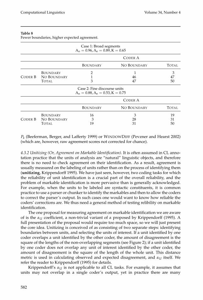
Computational Linguistics Volume 34, Number 4
Table 8Fewer boundaries, higher expected agreement.
Case 1: Broad segmentsAo = 0.96,Ae = 0.89, K = 0.65
CODER A
BOUNDARY NO BOUNDARY TOTAL
BOUNDARY 2 1 3CODER B NO BOUNDARY 1 46 47
TOTAL 3 47 50
Case 2: Fine discourse unitsAo = 0.88,Ae = 0.53, K = 0.75
CODER A
BOUNDARY NO BOUNDARY TOTAL
BOUNDARY 16 3 19CODER B NO BOUNDARY 3 28 31
TOTAL 19 31 50
Pk (Beeferman, Berger, and Lafferty 1999) or WINDOWDIFF (Pevzner and Hearst 2002)(which are, however, raw agreement scores not corrected for chance).
4.3.2 Unitizing (Or, Agreement on Markable Identification). It is often assumed in CL anno-tation practice that the units of analysis are “natural” linguistic objects, and thereforethere is no need to check agreement on their identification. As a result, agreement isusually measured on the labeling of units rather than on the process of identifying them(unitizing, Krippendorff 1995). We have just seen, however, two coding tasks for whichthe reliability of unit identification is a crucial part of the overall reliability, and theproblem of markable identification is more pervasive than is generally acknowledged.For example, when the units to be labeled are syntactic constituents, it is commonpractice to use a parser or chunker to identify themarkables and then to allow the codersto correct the parser’s output. In such cases one would want to know how reliable thecoders’ corrections are. We thus need a general method of testing relibility on markableidentification.
The one proposal for measuring agreement onmarkable identification we are awareof is the αU coefficient, a non-trivial variant of α proposed by Krippendorff (1995). Afull presentation of the proposal would require too much space, so we will just presentthe core idea. Unitizing is conceived of as consisting of two separate steps: identifyingboundaries between units, and selecting the units of interest. If a unit identified by onecoder overlaps a unit identified by the other coder, the amount of disagreement is thesquare of the lengths of the non-overlapping segments (see Figure 2); if a unit identifiedby one coder does not overlap any unit of interest identified by the other coder, theamount of disagreement is the square of the length of the whole unit. This distancemetric is used in calculating observed and expected disagreement, and αU itself. Werefer the reader to Krippendorff (1995) for details.
Krippendorff’s αU is not applicable to all CL tasks. For example, it assumes thatunits may not overlap in a single coder’s output, yet in practice there are many
582

Artstein and Poesio Inter-Coder Agreement for CL
Coder A
Coder Bs−✛ ✲ s✛ ✲ s+✛ ✲
Figure 2The difference between overlapping units is d(A, B) = s2− + s2+ (adapted from Krippendorff1995, Figure 4, page 61).
annotation schemes which require coders to label nested syntactic constituents. Forcontinuous segmentation tasks, αU may be inappropriate because when a segmentidentified by one annotator overlaps with two segments identified by another annotator,the distance is smallest when the one segment is centered over the two rather thanaligned with one of them. Nevertheless, we feel that when the non-overlap assumptionholds, and the units do not cover the text exhaustively, testing the reliabilty of unitidentification may prove beneficial. To our knowledge, this has never been tested in CL.
4.4 Anaphora
The annotation tasks discussed so far involve assigning a specific label to each category,which allows the various agreement measures to be applied in a straightforward way.Anaphoric annotation differs from the previous tasks because annotators do not assignlabels, but rather create links between anaphors and their antecedents. It is thereforenot clear what the “labels” should be for the purpose of calculating agreement. Onepossibility would be to consider the intended referent (real-world object) as the label,as in named entity tagging, but it wouldn’t make sense to predefine a set of “labels”applicable to all texts, because different objects are mentioned in different texts. Analternative is to use the marked antecedents as “labels”. However, we do not want tocount as a disagreement every time two coders agree on the discourse entity realizedby a particular noun phrase but just happen to mark different words as antecedents.Consider the reference of the underlined pronoun it in the following dialogue excerpt(TRAINS 1991 [Gross, Allen, and Traum 1993], dialogue d91-3.2).8
1.1 M: ....1.4 first thing I’d like you to do1.5 is send engine E2 off with a boxcar to Corning to
pick up oranges1.6 as soon as possible2.1 S: okay3.1 M: and while it’s there it should pick up the tanker
Some of the coders in a study we carried out (Poesio and Artstein 2005) indicated thenoun phrase engine E2 as antecedent for the second it in utterance 3.1, whereas othersindicated the immediately preceding pronoun, which they had previously marked ashaving engine E2 as antecedent. Clearly, we do not want to consider these coders to be indisagreement. A solution to this dilemma has been proposed by Passonneau (2004): Usethe emerging coreference sets as the ‘labels’ for the purpose of calculating agreement.This requires using weighted measures for calculating agreement on such sets, and
8 ftp://ftp.cs.rochester.edu/pub/papers/ai/92.tn1.trains 91 dialogues.txt.
583

Computational Linguistics Volume 34, Number 4
consequently it raises serious questions about weighted measures—in particular, aboutthe interpretability of the results, as we will see shortly.
4.4.1 Passonneau’s Proposal. Passonneau (2004) recommends measuring agreement onanaphoric annotation by using sets of mentions of discourse entities as labels, that is,the emerging anaphoric/coreference chains. This proposal is in line with the meth-ods developed to evaluate anaphora resolution systems (Vilain et al. 1995). But usinganaphoric chains as labels would not make unweighted measures such as K a goodmeasure for agreement. Practical experience suggests that, except when a text is veryshort, few annotators will catch all mentions of a discourse entity: Most will forget tomark a few, with the result that the chains (that is, category labels) differ from coderto coder and agreement as measured with K is always very low. What is needed isa coefficient that also allows for partial disagreement between judgments, when twoannotators agree on part of the coreference chain but not on all of it.
Passonneau (2004) suggests solving the problem by using α with a distance metricthat allows for partial agreement among anaphoric chains. Passonneau proposes a dis-tance metric based on the following rationale: Two sets are minimally distant when theyare identical andmaximally distant when they are disjoint; between these extremes, setsthat stand in a subset relation are closer (less distant) than ones that merely intersect.This leads to the following distance metric between two sets A and B.
dP =
0 if A = B1/3 if A ⊂ B or B ⊂ A2/3 if A ∩ B �= ∅, but A �⊂ B and B �⊂ A1 if A ∩ B = ∅
Alternative distance metrics take the size of the anaphoric chain into account, basedon measures used to compare sets in Information Retrieval, such as the coefficient ofcommunity of Jaccard (1912) and the coincidence index of Dice (1945) (Manning andSchutze 1999).
Jaccard: dJ = 1−|A ∩ B||A ∪ B|
Dice: dD = 1−2 |A ∩ B||A| + |B|
In later work, Passonneau (2006) offers a refined distance metric which she called MASI(Measuring Agreement on Set-valued Items), obtained by multiplying Passonneau’soriginal metric dP by the metric derived from Jaccard dJ .
dM = dP × dJ
4.4.2 Experience with α for Anaphoric Annotation. In the experiment mentioned previously(Poesio and Artstein 2005) we used 18 coders to test α and K under a variety of condi-tions.We found that even though our coders by and large agreed on the interpretation ofanaphoric expressions, virtually no coder ever identified all the mentions of a discourseentity. As a result, even though the values of α and K obtained by using the ID ofthe antecedent as label were pretty similar, the values obtained when using anaphoricchains as labels were drastically different. The value of α increased, because exampleswhere coders linked a markable to different antecedents in the same chain were no
584

Artstein and Poesio Inter-Coder Agreement for CL
longer considered as disagreements. However, the value of K was drastically reduced,because hardly any coder identified all the mentions of discourse entities (Figure 3).
The study also looked at the matter of individual annotator bias, and as mentionedin Section 3.1, we did not find differences between α and a κ-style version of α beyondthe third decimal point. This similarity is what one would expect, given the result aboutannotator bias from Section 3.1 and given that in this experiment we used 18 annotators.These very small differences should be contrasted with the differences resulting fromthe choice of distance metrics, where values for the full-chain condition ranged fromα = 0.642 using Jaccard as distance metric, to α = 0.654 using Passonneau’s metric, tothe value for Dice reported in Figure 3, α = 0.691. These differences raise an importantissue concerning the application of α-like measures for CL tasks: Using α makes it diffi-cult to compare the results of different annotation experiments, in that a “poor” value ora “high” valuemight result from “too strict” or “too generous” distancemetrics, makingit even more important to develop a methodology to identify appropriate values forthese coefficients. This issue is further emphasized by the study reported next.
4.4.3 Discourse Deixis. A second annotation study we carried out (Artstein and Poesio2006) shows even more clearly the possible side effects of using weighted coefficients.This study was concerned with the annotation of the antecedents of references toabstract objects, such as the example of the pronoun that in utterance 7.6 (TRAINS 1991,dialogue d91-2.2).
7.3 : so we ship one7.4 : boxcar7.5 : of oranges to Elmira7.6 : and that takes another 2 hours
Previous studies of discourse deixis annotation showed that these are extremely diffi-cult judgments to make (Eckert and Strube 2000; Navarretta 2000; Byron 2002), exceptperhaps for identifying the type of object (Poesio and Modjeska 2005), so we simplifiedthe task by only requiring our participants to identify the boundaries of the area oftext in which the antecedent was introduced. Even so, we found a great variety inhow these boundaries were marked: Exactly as in the case of discourse segmentationdiscussed earlier, our participants broadly agreed on the area of text, but disagreed on
Chain K α
None 0.628 0.656Partial 0.563 0.677Full 0.480 0.691
0.4
0.5
0.6
0.7
αα
α
K
K
K
no partial fullchain chain chain
Figure 3A comparison of the values of α and K for anaphoric annotation (Poesio and Artstein 2005).
585

Computational Linguistics Volume 34, Number 4
its exact boundary. For instance, in this example, nine out of ten annotators marked theantecedent of that as a text segment ending with the word Elmira, but some started withthe word so, some started with we, some with ship, and some with one.
We tested a number of ways tomeasure partial agreement on this task, and obtainedwidely different results. First of all, we tested three set-based distance metrics inspiredby the Passonneau proposals that we just discussed: We considered discourse segmentsto be sets of words, and computed the distance between them using Passonneau’smetric, Jaccard, and Dice. Using these three metrics, we obtained α values of 0.55 (withPassonneau’s metric), 0.45 (with Jaccard), and 0.55 (with Dice). We should note thatbecause antecedents of different expressions rarely overlapped, the expected disagree-ment was close to 1 (maximal), so the value of α turned out to be very close to the com-plement of the observed disagreement as calculated by the different distance metrics.
Next, we considered methods based on the position of words in the text. The firstmethod computed differences between absolute boundary positions: Each antecedentwas associated with the position of its first or last word in the dialogue, and agreementwas calculated using α with the interval distance metric. This gave us α values of0.998 for the beginnings of the antecedent-evoking area and 0.999 for the ends. This isbecause expected disagreement is exceptionally low: Coders tend to mark discourse an-tecedents close to the referring expression, so the average distance between antecedentsof the same expression is smaller than the size of the dialogue by a few orders ofmagnitude. The second method associated each antecedent with the position of itsfirst or last word relative to the beginning of the anaphoric expression. This time we foundextremely low values of α = 0.167 for beginnings of antecedents and 0.122 for ends—barely in the positive side. This shows that agreement among coders is not dramaticallybetter than what would be expected if they just marked discourse antecedents at a fixeddistance from the referring expression.
The three ranges of α that we observed (middle, high, and low) show agreement onthe identity of discourse antecedents, their position in the dialogue, and their positionrelative to referring expressions, respectively. The middle range shows variability of upto 10 percentage points, depending on the distance metric chosen. The lesson is thatonce we start using weighted measures we cannot anymore interpret the value of αusing traditional rules of thumb such as those proposed by Krippendorff or by Landisand Koch. This is because depending on the way we measure agreement, we can reportα values ranging from 0.122 to 0.998 for the very same experiment! New interpretationmethods have to be developed, which will be task- and distance-metric specific. We’llreturn to this issue in the conclusions.
4.5 Word Senses
Word sense tagging is one of the hardest annotation tasks. Whereas in the case of part-of-speech and dialogue act tagging the same categories are used to classify all units, inthe case of word sense tagging different categories must be used for each word, whichmakes writing a single codingmanual specifying examples for all categories impossible:The only option is to rely on a dictionary. Unfortunately, different dictionaries makedifferent distinctions, and often coders can’t make the fine-grained distinctions thattrained lexicographers can make. The problem is particularly serious for verbs, whichtend to be polysemous rather than homonymous (Palmer, Dang, and Fellbaum 2007).
These difficulties, and in particular the difficulty of tagging senses with a fine-grained repertoire of senses such as that provided by dictionaries or by WordNet(Fellbaum 1998), have been highlighted by the three SENSEVAL initiatives. Already
586

Artstein and Poesio Inter-Coder Agreement for CL
during the first SENSEVAL, Veronis (1998) carried out two studies of intercoderagreement on word sense tagging in the so-called ROMANSEVAL task. One study wasconcerned with agreement on polysemy—that is, the extent to which coders agreedthat a word was polysemous in a given context. Six naive coders were asked to makethis judgment about 600 French words (200 nouns, 200 verbs, 200 adjectives) using therepertoire of senses in the Petit Larousse. On this task, a (pairwise) percentage agreementof 0.68 for nouns, 0.74 for verbs, and 0.78 for adjectives was observed, correspondingto K values of 0.36, 0.37, and 0.67, respectively. The 20 words from each categoryperceived by the coders in this first experiment to be most polysemous were then usedin a second study, of intercoder agreement on the sense tagging task, which involvedsix different naive coders. Interestingly, the coders in this second experiment wereallowed to assign multiple tags to words, although they did not make much use of thispossibility; so κw was used to measure agreement. In this experiment, Veronis observed(weighted) pairwise agreement of 0.63 for verbs, 0.71 for adjectives, and 0.73 for nouns,corresponding to κw values of 0.41, 0.41, and 0.46, but with a wide variety of valueswhen measured per word—ranging from 0.007 for the adjective correct to 0.92 for thenoun detention. Similarly mediocre results for intercoder agreement between naivecoders were reported in the subsequent editions of SENSEVAL. Agreement studiesfor SENSEVAL-2, where WordNet senses were used as tags, reported a percentageagreement for verb senses of around 70%, whereas for SENSEVAL-3 (English LexicalSample Task), Mihalcea, Chklovski, and Kilgarriff (2004) report a percentage agreementof 67.3% and average K of 0.58.
Two types of solutions have been proposed for the problem of low agreement onsense tagging. The solution proposed by Kilgarriff (1999) is to use professional lexicog-raphers and arbitration. The study carried out by Kilgarriff does not therefore qualifyas a true study of replicability in the sense of the terms used by Krippendorff, but it didshow that this approach makes it possible to achieve percentage agreement of around95.5%. An alternative approach has been to address the problem of the inability of naivecoders to make fine-grained distinctions by introducing coarser-grained classificationschemes which group together dictionary senses (Bruce and Wiebe, 1998; Buitelaar1998; Veronis 1998; Palmer, Dang, and Fellbaum 2007). Hierarchical tagsets were alsodeveloped, such as HECTOR (Atkins 1992) or, indeed, WordNet itself (where senses arerelated by hyponymy links). In the case of Buitelaar and Palmer, Dang, and Fellbaum,the “supersenses” were identified by hand, whereas Bruce andWiebe and Veronis usedclustering methods such as those from Bruce and Wiebe (1999) to collapse some of theinitial sense distinctions.9 Palmer, Dang, and Fellbaum (2007) illustrate this practicewith the example of the verb call, which has 28 fine-grained senses in WordNet 1.7:They conflate these senses into a small number of groups using various criteria—forexample, four senses can be grouped in a group they call Group 1 on the basis ofsubcategorization frame similarities (Table 9).
Palmer, Dang, and Fellbaum (2007) achieved for the English Verb Lexical Sense taskof SENSEVAL-2 a percentage agreement among coders of 82% with grouped senses, asopposed to 71% with the original WordNet senses. Bruce and Wiebe (1998) found thatcollapsing the senses of their test word (interest) on the basis of their use by coders andmerging the two classes found to be harder to distinguish resulted in an increase of
9 The methodology proposed in Bruce and Wiebe (1999) is in our view the most advanced technique to“make sense” of the results of agreement studies available in the literature. The extended version of thisarticle contains a fuller introduction to these methods.
587

Computational Linguistics Volume 34, Number 4
Table 9Group 1 of senses of call in Palmer, Dang, and Fellbaum (2007, page 149).
SENSE DESCRIPTION EXAMPLE HYPERNYM
WN1 name, call “They nameda their son David” LABELWN3 call, give a quality “She called her children lazy LABEL
and ungrateful”WN19 call, consider “I would not call her beautiful” SEEWN22 address, call “Call me mister” ADDRESS
aThe verb named appears in the original WordNet example for the verb call.
the value of K from 0.874 to 0.898. Using a related technique, Veronis (1998) found thatagreement on noun word sense tagging went up from a K of around 0.45 to a K of 0.86.We should note, however, that the post hoc merging of categories is not equivalent torunning a study with fewer categories to begin with.
Attempts were also made to develop techniques to measure partial agreement withhierarchical tagsets. A first proposal in this direction was advanced by Melamed andResnik (2000), who developed a coefficient for hierarchical tagsets that could be usedin SENSEVAL for measuring agreement with tagsets such as HECTOR. Melamed andResnik proposed to “normalize” the computation of observed and expected agreementby taking each label which is not a leaf in the tag hierarchy and distributing it downto the leaves in a uniform way, and then only computing agreement on the leaves. Forexample, with a tagset like the one in Table 9, the cases in which the coders used thelabel ‘Group 1’ would be uniformly “distributed down” and added in equal measureto the number of cases in which the coders assigned each of the four WordNet labels.The method proposed in the paper has, however, problematic properties when usedto measure intercoder agreement. For example, suppose tag A dominates two sub-tagsA1 and A2, and that two coders mark a particular item as A. Intuitively, we would wantto consider this a case of perfect agreement, but this is not what the method proposedby Melamed and Resnik yields. The annotators’ marks are distributed over the twosub-tags, each with probability 0.5, and then the agreement is computed by summingthe joint probabilities over the two subtags (Equation (4) of Melamed and Resnik 2000),with the result that the agreement over the item turns out to be 0.52 + 0.52 = 0.5 insteadof 1. To correct this, Dan Melamed (personal communication) suggested replacing theproduct in Equation (4) with a minimum operator. However, the calculation of expectedagreement (Equation (5) of Melamed and Resnik 2000) still gives the amount of agree-ment which is expected if coders are forced to choose among leaf nodes, which makesthis method inappropriate for coding schemes that do not force coders to do this.
One way to use Melamed and Resnik’s proposal while avoiding the discrepancybetween observed and expected agreement is to treat the proposal not as a new co-efficient, but rather as a distance metric to be plugged into a weighted coefficientlike α. Let A and B be two nodes in a hierarchical tagset, let L be the set of all leafnodes in the tagset, and let P(l|T) be the probability of selecting a leaf node l givenan arbitrary node T when the probability mass of T is distributed uniformly to all thenodes dominated by T. We can reinterpret Melamed’s modification of Equation (4) inMelamed and Resnik (2000) as a metric measuring the distance between nodes A and B.
dM+R = 1− ∑l∈L
min(P(l|A), P(l|B))
588
Artstein and Poesio Inter-Coder Agreement for CL
This metric has the desirable properties—it is 0 when tags A and B are identical,1 when the tags do not overlap, and somewhere in between in all other cases. If weuse this metric for Krippendorff’s α we find that observed agreement is exactly thesame as inMelamed and Resnik (2000) with the product operator replaced byminimum(Melamed’s modification).
We can also use other distance metrics with α. For example, we could associatewith each sense an extended sense—a set es(s) including the sense itself and itsgrouped sense—and then use set-based distance metrics from Section 4.4, for ex-ample Passonneau’s dP. To illustrate how this approach could be used to measure(dis)agreement on word sense annotation, suppose that two coders have to annotate theuse of call in the following sentence (from theWSJ part of the Penn Treebank, section 02,text w0209):
This gene, called “gametocide,” is carried into the plant by a virus thatremains active for a few days.
The standard guidelines (in SENSEVAL, say) require coders to assign a WN sense towords. Under such guidelines, if coder A classifies the use of called in the above exampleas an instance of WN1, whereas coder B annotates it as an instance of WN3, we wouldfind total disagreement (dkakb
= 1) which seems excessively harsh as the two senses areclearly related. However, by using the broader senses proposed by Palmer, Dang, andFellbaum (2007) in combination with a distance metric such as the one just proposed,it is possible to get more flexible and, we believe, more realistic assessments of thedegree of agreement in situations such as this. For instance, in case the reliability studyhad already been carried out under the standard SENSEVAL guidelines, the distancemetric proposed above could be used to identify post hoc cases of partial agreementby adding to each WN sense its hypernyms according to the groupings proposed byPalmer, Dang, and Fellbaum. For example, A’s annotation could be turned into a newset label {WN1,LABEL} and B’s mark into the set table {WN3,LABEL}, which wouldgive a distance d = 2/3, indicating a degree of overlap. The method for computingagreement proposed here could could also be used to allow coders to choose either amore specific label or one of Palmer, Dang, and Fellbaum’s superlabels. For example,suppose A sticks to WN1, but B decides to mark the use above using Palmer, Dang, andFellbaum’s LABEL category, then we would still find a distance d = 1/3.
An alternative way of using α for word sense annotation was developed and testedby Passonneau, Habash, and Rambow (2006). Their approach is to allow coders toassign multiple labels (WordNet synsets) for wordsenses, as done by Veronis (1998) andmore recently by Rosenberg and Binkowski (2004) for text classification labels and byPoesio and Artstein (2005) for anaphora. These multi-label sets can then be comparedusing the MASI distance metric for α (Passonneau 2006).
5. Conclusions
The purpose of this article has been to expose the reader to the mathematics of chance-corrected coefficients of agreement as well as the current state of the art of using thesecoefficients in CL. Our hope is that readers come to view agreement studies not as anadditional chore or hurdle for publication, but as a tool for analysis which offers newinsights into the annotation process. We conclude by summarizing what in our view arethe main recommendations emerging from ten years of experience with coefficients ofagreement. These can be grouped under three main headings: methodology, choice ofcoefficients, and interpretation of coefficients.
589

Computational Linguistics Volume 34, Number 4
5.1 Methodology
Our first recommendation is that annotation efforts should perform and report rigorousreliability testing. The last decade has already seen considerable improvement, fromthe absence of any tests for the Penn Treebank (Marcus, Marcinkiewicz, and Santorini1993) or the British National Corpus (Leech, Garside, and Bryant 1994) to the centralrole played by reliability testing in the Penn Discourse Treebank (Miltsakaki et al. 2004)and OntoNotes (Hovy et al. 2006). But even the latter efforts only measure and reportpercent agreement. We believe that part of the reluctance to report chance-correctedmeasures is the difficulty in interpreting them. However, our experience is that chance-corrected coefficients of agreement do provide a better indication of the quality of theresulting annotation than simple percent agreement, and moreover, the detailed calcu-lations leading to the coefficients can be very revealing as to where the disagreementsare located and what their sources may be.
A rigorous methodology for reliability testing does not, in our opinion, exclude theuse of expert coders, and here we feel there may be a motivated difference between thefields of content analysis and CL. There is a clear tradeoff between the complexity ofthe judgments that coders are required to make and the reliability of such judgments,and we should strive to devise annotation schemes that are not only reliable enoughto be replicated, but also sophisticated enough to be useful (cf. Krippendorff 2004a,pages 213–214). In content analysis, conclusions are drawn directly from annotatedcorpora, so the emphasis is more on replicability; whereas in CL, corpora constitute aresource which is used by other processes, so the emphasis is more towards usefulness.There is also a tradeoff between the sophistication of judgments and the availability ofcoders who can make such judgments. Consequently, annotation by experts is oftenthe only practical way to get useful corpora for CL. Current practice achieves highreliability either by using professionals (Kilgarriff 1999) or through intensive training(Hovy et al. 2006; Carlson, Marcu, and Okurowski 2003); this means that results are notreplicable across sites, and are therefore less reliable than annotation by naive codersadhering to written instructions. We feel that inter-annotator agreement studies shouldstill be carried out, as they serve as an assurance that the results are replicable whenthe annotators are chosen from the same population as the original annotators. Animportant additional assurance should be provided in the form of an independentevaluation of the task for which the corpus is used (cf. Passonneau 2006).
5.2 Choosing a Coefficient
One of the goals of this article is to help authors make an informed choice regardingthe coefficients they use for measuring agreement. While coefficients other than K,specifically Cohen’s κ and Krippendorff’s α, have appeared in the CL literature as earlyas Carletta (1996) and Passonneau and Litman (1996), they hadn’t sprung into generalawareness until the publication of Di Eugenio and Glass (2004) and Passonneau (2004).Regarding the question of annotator bias, there is an overwhelming consensus in CLpractice: K and α are used in the vast majority of the studies we reported. We agree withthe view that K and α are more appropriate, as they abstract away from the bias of spe-cific coders. But we also believe that ultimately this issue of annotator bias is of little con-sequence because the differences get smaller and smaller as the number of annotatorsgrows (Artstein and Poesio 2005). We believe that increasing the number of annotatorsis the best strategy, because it reduces the chances of accidental personal biases.
590
Artstein and Poesio Inter-Coder Agreement for CL
However, Krippendorff’s α is indispensable when the category labels are notequally distinct from one another. We think there are at least two types of codingschemes in which this is the case: (i) hierarchical tagsets and (ii) set-valued interpre-tations such as those proposed for anaphora. At least in the second case, weightedcoefficients are almost unavoidable. We therefore recommend using α, noting howeverthat the specific choice of weights will affect the overall numerical result.
5.3 Interpreting the Values
We view the lack of consensus on how to interpret the values of agreement coefficientsas a serious problem with current practice in reliability testing, and as one of themain reasons for the reluctance of many in CL to embark on reliability studies. Unlikesignificance values which report a probability (that an observed effect is due to chance),agreement coefficients report a magnitude, and it is less clear how to interpret suchmagnitudes. Our own experience is consistent with that of Krippendorff: Both in ourearlier work (Poesio and Vieira 1998; Poesio 2004a) and in the more recent efforts(Poesio and Artstein 2005) we found that only values above 0.8 ensured an annotationof reasonable quality (Poesio 2004a). We therefore feel that if a threshold needs to be set,0.8 is a good value.
That said, we doubt that a single cutoff point is appropriate for all purposes.For some CL studies, particularly on discourse, useful corpora have been obtainedwhile attaining reliability only at the 0.7 level. We agree therefore with Craggs andMcGee Wood (2005) that setting a specific agreement threshold should not be a pre-requisite for publication. Instead, as recommended by Di Eugenio and Glass (2004) andothers, researchers should report in detail on the methodology that was followed incollecting the reliability data (number of coders, whether they coded independently,whether they relied exclusively on an annotation manual), whether agreement was sta-tistically significant, and provide a confusion matrix or agreement table so that readerscan find out whether overall figures of agreement hide disagreements on less commoncategories. For an example of good practice in this respect, see Teufel and Moens (2002).The decision whether a corpus is good enough for publication should be based on morethan the agreement score—specifically, an important consideration is an independentevaluation of the results that are based on the corpus.
AcknowledgmentsThis work was supported in part by EPSRCgrant GR/S76434/01, ARRAU. We wish tothank four anonymous reviewers and JeanCarletta, Mark Core, Barbara Di Eugenio,Ruth Filik, Michael Glass, George Hripcsak,Adam Kilgarriff, Dan Melamed, BeckyPassonneau, Phil Resnik, Tony Sanford,Patrick Sturt, and David Traum for helpfulcomments and discussion. Special thanks toKlaus Krippendorff for an extremely detailedreview of an earlier version of this article. Weare also extremely grateful to the BritishLibrary in London, which made accessible tous virtually every paper we needed for thisresearch.
ReferencesAllen, James and Mark Core. 1997. DAMSL:Dialogue act markup in several layers.Draft contribution for the DiscourseResource Initiative, University ofRochester. Available athttp://www.cs.rochester.edu/research/cisd/resources/damsl/.
Artstein, Ron and Massimo Poesio. 2005.Bias decreases in proportion to the numberof annotators. In Proceedings of FG-MoL2005, pages 141–150, Edinburgh.
Artstein, Ron and Massimo Poesio. 2006.Identifying reference to abstract objectsin dialogue. In brandial 2006: Proceedingsof the 10th Workshop on the Semantics and
591

Computational Linguistics Volume 34, Number 4
Pragmatics of Dialogue, pages 56–63,Potsdam.
Atkins, Sue. 1992. Tools for computer-aidedcorpus lexicography: The Hector project.Acta Linguistica Hungarica, 41:5–71.
Babarczy, Anna, John Carroll, and GeoffreySampson. 2006. Definitional, personal,and mechanical constraints on partof speech annotation performance.Natural Language Engineering, 12(1):77–90.
Bartko, John J. and William T. Carpenter, Jr.1976. On the methods and theory ofreliability. Journal of Nervous and MentalDisease, 163(5):307–317.
Beeferman, Doug, Adam Berger, andJohn Lafferty. 1999. Statistical modelsfor text segmentation. Machine Learning,34(1–3):177–210.
Bennett, E. M., R. Alpert, and A. C.Goldstein. 1954. Communicationsthrough limited questioning. PublicOpinion Quarterly, 18(3):303–308.
Bloch, Daniel A. and Helena ChmuraKraemer. 1989. 2 × 2 kappa coefficients:Measures of agreement or association.Biometrics, 45(1):269–287.
Brennan, Robert L. and Dale J. Prediger.1981. Coefficient kappa: Some uses,misuses, and alternatives. Educationaland Psychological Measurement,41(3):687–699.
Bruce, Rebecca and Janyce Wiebe. 1998.Word-sense distinguishability andinter-coder agreement. In Proceedingsof EMNLP, pages 53–60, Granada.
Bruce, Rebecca F. and Janyce M. Wiebe. 1999.Recognizing subjectivity: A case study inmanual tagging. Natural LanguageEngineering, 5(2):187–205.
Buitelaar, Paul. 1998. CoreLex : SystematicPolysemy and Underspecification. Ph.D.thesis, Brandeis University, Waltham, MA.
Bunt, Harry C. 2000. Dynamic interpretationand dialogue theory. In Martin M. Taylor,Francoise Neel, and Don G. Bouwhuis,editors, The Structure of MultimodalDialogue II. John Benjamins, Amsterdam,pages 139–166.
Bunt, Harry C. 2005. A framework fordialogue act specification. In Proceedingsof the Joint ISO-ACL Workshop on theRepresentation and Annotation of SemanticInformation, Tilburg. Available at:http://let.uvt.nl/research/ti/sigsem/wg/discussionnotes4.htm.
Byron, Donna K. 2002. Resolvingpronominal reference to abstract entities.In Proceedings of the 40th Annual Meeting ofthe ACL, pages 80–87, Philadelphia, PA.
Byrt, Ted, Janet Bishop, and John B. Carlin.1993. Bias, prevalence and kappa. Journalof Clinical Epidemiology, 46(5):423–429.
Carletta, Jean. 1996. Assessing agreement onclassification tasks: The kappa statistic.Computational Linguistics, 22(2):249–254.
Carletta, Jean, Amy Isard, Stephen Isard,Jacqueline C. Kowtko, GwynethDoherty-Sneddon, and Anne H.Anderson. 1997. The reliability of adialogue structure coding scheme.Computational Linguistics, 23(1):13–32.
Carlson, Lynn, Daniel Marcu, andMary Ellen Okurowski. 2003. Building adiscourse-tagged corpus in the frameworkof rhetorical structure theory. In Jan C. J.van Kuppevelt and Ronnie W. Smith,editors, Current and New Directions inDiscourse and Dialogue. Kluwer, Dordrecht,pages 85–112.
Cicchetti, Domenic V. and Alvan R.Feinstein. 1990. High agreement but lowkappa: II. Resolving the paradoxes. Journalof Clinical Epidemiology, 43(6):551–558.
Cohen, Jacob. 1960. A coefficient ofagreement for nominal scales. Educationaland Psychological Measurement, 20(1):37–46.
Cohen, Jacob. 1968. Weighted kappa:Nominal scale agreement with provisionfor scaled disagreement or partial credit.Psychological Bulletin, 70(4):213–220.
Core, Mark G. and James F. Allen. 1997.Coding dialogs with the DAMSLannotation scheme. In Working Notes of theAAAI Fall Symposium on CommunicativeAction in Humans and Machines, AAAI,Cambridge, MA. Available at: http://www.cs.umd.edu/∼traum/CA/fpapers.html.
Craggs, Richard and Mary McGee Wood.2004. A two-dimensional annotationscheme for emotion in dialogue. In Papersfrom the 2004 AAAI Spring Symposium onExploring Attitude and Affect in Text:Theories and Applications, Stanford,pages 44–49.
Craggs, Richard and Mary McGee Wood.2005. Evaluating discourse and dialoguecoding schemes. Computational Linguistics,31(3):289–295.
Davies, Mark and Joseph L. Fleiss. 1982.Measuring agreement for multinomialdata. Biometrics, 38(4):1047–1051.
Di Eugenio, Barbara. 2000. On the usage ofKappa to evaluate agreement on codingtasks. In Proceedings of LREC, volume 1,pages 441–444, Athens.
Di Eugenio, Barbara and Michael Glass.2004. The kappa statistic: A second look.Computational Linguistics, 30(1):95–101.
592

Artstein and Poesio Inter-Coder Agreement for CL
Di Eugenio, Barbara, Pamela W. Jordan,Johanna D. Moore, and Richmond H.Thomason. 1998. An empiricalinvestigation of proposals in collaborativedialogues. In Proceedings of 36th AnnualMeeting of the ACL, pages 325–329,Montreal.
Dice, Lee R. 1945. Measures of the amountof ecologic association between species.Ecology, 26(3):297–302.
Donner, Allan and Michael Eliasziw.1987. Sample size requirements forreliability studies. Statistics in Medicine,6:441–448.
Doran, Christine, John Aberdeen, LaurieDamianos, and Lynette Hirschman.2001. Comparing several aspects ofhuman-computer and human-humandialogues. In Proceedings of the 2ndSIGdial Workshop on Discourse andDialogue, Aalborg, Denmark. Available at:http://www.sigdial.org/workshops/workshop2/proceedings.
Eckert, Miriam and Michael Strube. 2000.Dialogue acts, synchronizing units,and anaphora resolution. Journal ofSemantics, 17(1):51–89.
Feinstein, Alvan R. and Domenic V. Cicchetti.1990. High agreement but low kappa:I. The problems of two paradoxes. Journalof Clinical Epidemiology, 43(6):543–549.
Fellbaum, Christiane, editor. 1998. WordNet:An Electronic Lexical Database. MIT Press,Cambridge, MA.
Fleiss, Joseph L. 1971. Measuring nominalscale agreement among many raters.Psychological Bulletin, 76(5):378–382.
Fleiss, Joseph L. 1975. Measuring agreementbetween two judges on the presence orabsence of a trait. Biometrics, 31(3):651–659.
Francis, W. Nelson and Henry Kucera.1982. Frequency Analysis of English Usage:lexicon and grammar. Houghton Mifflin,Boston, MA.
Geertzen, Jeroen and Harry Bunt. 2006.Measuring annotator agreement in acomplex hierarchical dialogue actannotation scheme. In Proceedings of the7th SIGdial Workshop on Discourse andDialogue, pages 126–133, Sydney.
Gross, Derek, James F. Allen, and David R.Traum. 1993. The Trains 91 dialogues.TRAINS Technical Note 92-1, Universityof Rochester Computer ScienceDepartment, Rochester, NY.
Grosz, Barbara J. and Candace L. Sidner.1986. Attention, intentions, and thestructure of discourse. ComputationalLinguistics, 12(3):175–204.
Hayes, Andrew F. and Klaus Krippendorff.2007. Answering the call for a standardreliability measure for coding data.Communication Methods and Measures,1(1):77–89.
Hearst, Marti A. 1997. TextTiling:Segmenting text into multi-paragraphsubtopic passages. ComputationalLinguistics, 23(1):33–64.
Hovy, Eduard, Mitchell Marcus, MarthaPalmer, Lance Ramshaw, and RalphWeischedel. 2006. OntoNotes: The 90%solution. In Proceedings of HLT–NAACL,Companion Volume: Short Papers,pages 57–60, New York.
Hsu, Louis M. and Ronald Field. 2003.Interrater agreement measures: Commentson kappan, Cohen’s kappa, Scott’s π,and Aickin’s α. Understanding Statistics,2(3):205–219.
Jaccard, Paul. 1912. The distribution of theflora in the Alpine zone. New Phytologist,11(2):37–50.
Jekat, Susanne, Alexandra Klein, ElisabethMaier, Ilona Maleck, Marion Mast, andJ. Joachim Quantz. 1995. Dialogue acts inVERBMOBIL. VM-Report 65, UniversitatHamburg, DFKI GmbH, UniversitatErlangen, and TU Berlin.
Jurafsky, Daniel, Elizabeth Shriberg, andDebra Biasca. 1997. SwitchboardSWBD-DAMSL shallow-discourse-function annotation coders manual,draft 13. Technical Report 97-02,University of Colorado at Boulder,Institute for Cognitive Science.
Kilgarriff, Adam. 1999. 95% replicabilityfor manual word sense tagging. InProceedings of the Ninth Conferenceof the European Chapter of the Associationfor Computational Linguistics,pages 277–278, Bergen, Norway.
Klavans, Judith L., Samuel Popper, andRebecca Passonneau. 2003. Tacklingthe internet glossary glut: Automaticextraction and evaluation of genusphrases. In Proceedings of theSIGIR-2003 Workshop on the Semantic Web,Toronto.
Kowtko, Jacqueline C., Stephen D. Isard,and Gwyneth M. Doherty. 1992.Conversational games within dialogue.Research Paper HCRC/RP-31, HumanCommunication Research Centre,University of Edinburgh.
Krippendorff, Klaus. 1970. Estimating thereliability, systematic error and randomerror of interval data. Educational andPsychological Measurement, 30(1):61–70.
593

Computational Linguistics Volume 34, Number 4
Krippendorff, Klaus. 1978. Reliability ofbinary attribute data. Biometrics,34(1):142–144. Letter to the editor,with a reply by Joseph L. Fleiss.
Krippendorff, Klaus. 1980. Content Analysis:An Introduction to Its Methodology,chapter 12. Sage, Beverly Hills, CA.
Krippendorff, Klaus. 1995. On the reliabilityof unitizing contiguous data. SociologicalMethodology, 25:47–76.
Krippendorff, Klaus. 2004a. Content Analysis:An Introduction to Its Methodology,second edition, chapter 11. Sage,Thousand Oaks, CA.
Krippendorff, Klaus. 2004b. Reliabilityin content analysis: Some commonmisconceptions and recommendations.Human Communication Research,30(3):411–433.
Landis, J. Richard and Gary G. Koch. 1977.The measurement of observer agreementfor categorical data. Biometrics,33(1):159–174.
Leech, Geoffrey, Roger Garside, and MichaelBryant. 1994. CLAWS4: The tagging of theBritish National Corpus. In Proceedings ofCOLING 1994: The 15th InternationalConference on Computational Linguistics,Volume 1, pages 622–628, Kyoto.
Levin, James A. and James A. Moore. 1978.Dialogue-games: Metacommunicationstructures for natural languageinteraction. Cognitive Science, 1(4):395–420.
Manning, Christopher D. and HinrichSchuetze. 1999. Foundations of StatisticalNatural Language Processing. MIT Press,Cambridge, MA.
Marcu, Daniel, Magdalena Romera, andEstibaliz Amorrortu. 1999. Experiments inconstructing a corpus of discourse trees:Problems, annotation choices, issues. InWorkshop on Levels of Representation inDiscourse, pages 71–78, University ofEdinburgh.
Marcus, Mitchell P., Mary AnnMarcinkiewicz, and Beatrice Santorini.1993. Building a large annotated corpus ofEnglish: the Penn Treebank. ComputationalLinguistics, 19(2):313–330.
Marion, Rodger. 2004. The whole art ofdeduction. Unpublished manuscript.
Melamed, I. Dan and Philip Resnik. 2000.Tagger evaluation given hierarchicaltagsets. Computers and the Humanities,34(1–2):79–84. Available at:http://www.sahs/utmb.edu/PELLINORE/Intro to research/wad/wad/ home.htm.
Mieskes, Margot and Michael Strube. 2006.Part-of-speech tagging of transcribed
speech. In Proceedings of LREC,pages 935–938, Genoa.
Mihalcea, Rada, Timothy Chklovski, andAdam Kilgarriff. 2004. The SENSEVAL-3English lexical sample task. In Proceedingsof SENSEVAL-3, pages 25–28, Barcelona.
Miltsakaki, Eleni, Rashmi Prasad, AravindJoshi, and Bonnie Webber. 2004.Annotating discourse connectivesand their arguments. In Proceedingsof the HLT-NAACL Workshop onFrontiers in Corpus Annotation, pages 9–16,Boston, MA.
Moser, Megan G., Johanna D. Moore, andErin Glendening. 1996. Instructionsfor Coding Explanations: IdentifyingSegments, Relations and Minimal Units.Technical Report 96-17, University ofPittsburgh, Department of ComputerScience.
Navarretta, Costanza. 2000. Abstractanaphora resolution in Danish. InProceedings of the 1st SIGdial Workshop onDiscourse and Dialogue, Hong Kong,pages 56–65.
Nenkova, Ani and Rebecca Passonneau.2004. Evaluating content selection insummarization: The pyramid method.In Proceedings of HLT-NAACL 2004,pages 145–152, Boston, MA.
Neuendorf, Kimberly A. 2002. TheContent Analysis Guidebook. Sage,Thousand Oaks, CA.
Palmer, Martha, Hoa Trang Dang, andChristiane Fellbaum. 2007. Makingfine-grained and coarse-grained sensedistinctions, both manually andautomatically. Natural LanguageEngineering, 13(2):137–163.
Passonneau, Rebecca J. 2004. Computingreliability for coreference annotation.In Proceedings of LREC, volume 4,pages 1503–1506, Lisbon.
Passonneau, Rebecca J. 2006. Measuringagreement on set-valued items (MASI)for semantic and pragmatic annotation.In Proceedings of LREC, Genoa,pages 831–836.
Passonneau, Rebecca J., Nizar Habash, andOwen Rambow. 2006. Inter-annotatoragreement on a multilingual semanticannotation task. In Proceedings of LREC,Genoa, pages 1951–1956.
Passonneau, Rebecca J. and Diane J. Litman.1993. Intention-based segmentation:Human reliability and correlation withlinguistic cues. In Proceedings of 31stAnnual Meeting of the ACL, pages 148–155,Columbus, OH.
594

Artstein and Poesio Inter-Coder Agreement for CL
Passonneau, Rebecca J. and Diane J. Litman.1996. Empirical analysis of threedimensions of spoken discourse:Segmentation, coherence and linguisticdevices. In Eduard H. Hovy and DoniaR. Scott, editors, Computational andConversational Discourse: Burning Issues –An Interdisciplinary Account, volume 151of NATO ASI Series F: Computer andSystems Sciences. Springer, Berlin,chapter 7, pages 161–194.
Passonneau, Rebecca J. and Diane J. Litman.1997. Discourse segmentation by humanand automated means. ComputationalLinguistics, 23(1):103–139.
Pevzner, Lev and Marti A. Hearst. 2002.A critique and improvement of anevaluation metric for text segmentation.Computational Linguistics, 28(1):19–36.
Poesio, Massimo. 2004a. Discourseannotation and semantic annotation in theGNOME corpus. In Proceedings of the 2004ACL Workshop on Discourse Annotation,pages 72–79, Barcelona.
Poesio, Massimo. 2004b. TheMATE/GNOME proposals for anaphoricannotation, revisited. In Proceedings of the5th SIGdial Workshop on Discourse andDialogue, pages 154–162, Cambridge, MA.
Poesio, Massimo and Ron Artstein. 2005.The reliability of anaphoric annotation,reconsidered: Taking ambiguity intoaccount. In Proceedings of the Workshop onFrontiers in Corpus Annotation II: Pie in theSky, pages 76–83, Ann Arbor, MI.
Poesio, Massimo and Natalia N. Modjeska.2005. Focus, activation, and this-nounphrases: An empirical study. InAntonio Branco, Tony McEnery, andRuslan Mitkov, editors, AnaphoraProcessing, volume 263 of Current Issuesin Linguistic Theory. John Benjamins,pages 429–442, Amsterdam andPhiladelphia.
Poesio, Massimo, A. Patel, and BarbaraDi Eugenio. 2006. Discourse structureand anaphora in tutorial dialogues: Anempirical analysis of two theories of theglobal focus. Research in Language andComputation, 4(2–3):229–257.
Poesio, Massimo and Renata Vieira. 1998.A corpus-based investigation of definitedescription use. Computational Linguistics,24(2):183–216.
Popescu-Belis, Andrei. 2005. Dialogue acts:One or more dimensions? WorkingPaper 62, ISSCO, University of Geneva.
Posner, Karen L., Paul D. Sampson, Robert A.Caplan, Richard J. Ward, and Frederick W.
Cheney. 1990. Measuring interraterreliability among multiple raters: Anexample of methods for nominal data.Statistics in Medicine, 9:1103–1115.
Rajaratnam, Nageswari. 1960. Reliabilityformulas for independent decision datawhen reliability data are matched.Psychometrika, 25(3):261–271.
Reidsma, Dennis and Jean Carletta. 2008.Reliability measurement without limits.Computational Linguistics, 34(3):319–326.
Reinhart, T. 1981. Pragmatics and linguistics:An analysis of sentence topics.Philosophica, 27(1):53–93.
Reynar, Jeffrey C. 1998. Topic Segmentation:Algorithms and Applications. Ph.D. thesis,University of Pennsylvania, Philadelphia.
Ries, Klaus. 2002. Segmenting conversationsby topic, initiative and style. In Anni R.Coden, Eric W. Brown, and SavithaSrinivasan, editors, Information RetrievalTechniques for Speech Applications,volume 2273 of Lecture Notes in ComputerScience. Springer, Berlin, pages 51–66.
Rietveld, Toni and Roeland van Hout.1993. Statistical Techniques for the Studyof Language and Language Behaviour.Mouton de Gruyter, Berlin.
Rosenberg, Andrew and Ed Binkowski.2004. Augmenting the kappa statisticto determine interannotator reliabilityfor multiply labeled data points. InProceedings of HLT-NAACL 2004: ShortPapers, pages 77–80, Boston, MA.
Scott, William A. 1955. Reliability of contentanalysis: The case of nominal scalecoding. Public Opinion Quarterly,19(3):321–325.
Shriberg, Elizabeth, Raj Dhillon, SonaliBhagat, Jeremy Ang, and Hannah Carvey.2004. The ICSI meeting recorder dialog act(MRDA) corpus. In Proceedings of the 5thSIGdial Workshop on Discourse and Dialogue,pages 97–100, Cambridge, MA.
Siegel, Sidney and N. John Castellan, Jr. 1988.Nonparametric Statistics for the BehavioralSciences, 2nd edition, chapter 9.8.McGraw-Hill, New York.
Stent, Amanda J. 2001. Dialogue Systemsas Conversational Partners: ApplyingConversation Acts Theory to NaturalLanguage Generation for Task-OrientedMixed-Initiative Spoken Dialogue. Ph.D.thesis, Department of Computer Science,University of Rochester.
Stevenson, Mark and Robert Gaizauskas.2000. Experiments on sentence boundarydetection. In Proceedings of 6th ANLP,pages 84–89, Seattle, WA.
595
Computational Linguistics Volume 34, Number 4
Stolcke, Andreas, Noah Coccaro, RebeccaBates, Paul Taylor, Carol Van Ess-Dykema,Klaus Ries, Elizabeth Shriberg, DanielJurafsky, Rachel Martin, and Marie Meteer.2000. Dialogue act modeling for automatictagging and recognition of conversationalspeech. Computational Linguistics,26(3):339–373.
Stuart, Alan. 1955. A test for homogeneity ofthe marginal distributions in a two-wayclassification. Biometrika, 42(3/4):412–416.
Teufel, Simone, Jean Carletta, and MarcMoens. 1999. An annotation schemefor discourse-level argumentation inresearch articles. In Proceedings of NinthConference of the EACL, pages 110–117,Bergen.
Teufel, Simone and Marc Moens. 2002.Summarizing scientific articles:Experiments with relevance andrhetorical status. ComputationalLinguistics, 28(4):409–445.
Traum, David R. and Elizabeth A.Hinkelman. 1992. Conversationacts in task-oriented spoken dialogue.Computational Intelligence, 8(3):575–599.
Vallduvı, Enric. 1993. Informationpackaging: A survey. Research PaperRP-44, University of Edinburgh, HCRC.
Veronis, Jean. 1998. A study of polysemyjudgments and inter-annotator agreement.In Proceedings of SENSEVAL-1,Herstmonceux Castle, England. Availableat: http://www.itri.brighton.ac.uk/events/senseval/ARCHIVE/PROCEEDINGS/.
Vilain, Marc, John Burger, John Aberdeen,Dennis Connolly, and Lynette Hirschman.1995. A model-theoretic coreferencescoring scheme. In Proceedings of the SixthMessage Understanding Conference,pages 45–52, Columbia, MD.
Zwick, Rebecca. 1988. Another look atinterrater agreement. PsychologicalBulletin, 103(3):374–378.
596