Surrogate Modelling for Injection Molding Processes using Machine

Learning

Arsenii Uglova,, Sergei Nikolaeva,, Sergei Belova, Daniil Padalitsaa, Tatiana Greenkinaa,Marco San Biagio, Fabio Cacciatorib

aSkolkovo Institute of Science and Technology, Bolshoy Boulevard 30, bld. 1, Moscow, 121205, RussiabIllogic s.r.l, Corso stati Uniti 57,10128, Turin, Italy

Abstract

Injection molding is one of the most popular manufacturing methods for the modeling ofcomplex plastic objects. Faster numerical simulation of the technological process would allowfor faster and cheaper design cycles of new products. In this work, we propose a baselinefor a data processing pipeline that includes the extraction of data from Moldflow simulationprojects and the prediction of the fill time and deflection distributions over 3-dimensionalsurfaces using machine learning models. We propose algorithms for engineering of features,including information of injector gates parameters that will mostly affect the time for plasticto reach the particular point of the form for fill time prediction, and geometrical features fordeflection prediction. We propose and evaluate baseline machine learning models for fill timeand deflection distribution prediction and provide baseline values of MSE and RMSE metrics.Finally, we measure the execution time of our solution and show that it significantly exceedsthe time of simulation with Moldflow software: approximately 17 times and 14 times fasterfor mean and median total times respectively, comparing the times of all analysis stages fordeflection prediction. Our solution has been implemented in a prototype web applicationthat was approved by the management board of Fiat Chrysler Automobiles and Illogic SRL.As one of the promising applications of this surrogate modelling approach, we envision theuse of trained models as a fast objective function in the task of optimization of technologicalparameters of the injection molding process (meaning optimal placement of gates), whichcould significantly aid engineers in this task, or even automate it.

Keywords: injection molding, surrogate modeling, machine learning, baseline, deeplearning, Autodesk Moldflow, 3d machine learning, 3d data, mesh, point cloud, fluiddynamics simulation

1. Introduction

Injection molding is a widespread manufacturing process for producing objects of givenshapes from various materials. It is the most common modern method of manufacturingof plastic parts, and it is ideal for producing high volumes of copies of the same object.

Email addresses: urrusmsng@gmail.com (Arsenii Uglov), s.nikolaev@skoltech.ru (Sergei Nikolaev),marco.sanbiagio@gmail.com (Marco San Biagio), cacciatori@illogic.xyz (Fabio Cacciatori)

1

arX

iv:2

107.

1457

4v1

[cs

.LG

] 3

0 Ju

l 202

1

Numerical analysis is crucial for designing products with given mechanical properties and aminimal number of defects. The industry standard is to use extensive fluid-dynamics-basedsimulations with specialized software such as Autodesk Moldflow. This kind of simulationis computationally quite burdensome and time-consuming. As well, the final result is highlydependent on the experience and skills of the engineers, introducing variance in quality. Somemanufacturers are interested in shorter and cheaper design cycles with less human interaction.

One way to accelerate a design cycle and expand searchable design space is to implementsurrogate-based optimization [1]. Data-driven models such as Gaussian processes, supportvector machines (SVM) and artificial neural networks (ANN) are common choices for surro-gate models.

In recent years, we have observed a steady rise in interest in the application of deeplearning (DL) models to model physical or engineering processes. For example, generativeadversarial networks (GANs) are used in high energy-physics for fast approximate simulationof detector responses [2, 3], and supervised DL architectures are used in geology for real-timesimulation of seismic waves [4] and for semiconductor manufacturing [5].

In this work we consider a deep learning approach to creating a surrogate model, basedon Moldflow simulation data, which predicts the distribution of fill time and deflection valuesover the 3d surface as targets of the simulation.

Our research into related works on this topic has, as of 2020, found no description of asimilar approach for the described task, so we consider our results to be a baseline.

This work was created as a part of a project with an Italian automotive industry part-ner Fiat Chrysler Automobiles. They provided us with a dataset of Moldflow project filesof simulations. Since this work is covered by the non-disclosure agreement, including thedataset, we cannot disclose the partner’s name or provide many vivid data representations,as the format of the data suggests. However, we will provide summary details of a dataset, adescription of the used features, details of our data processing pipeline and machine learning(ML) models, and the achieved values of the result metrics.

2. Injection Molding Process

2.1. Molding Process

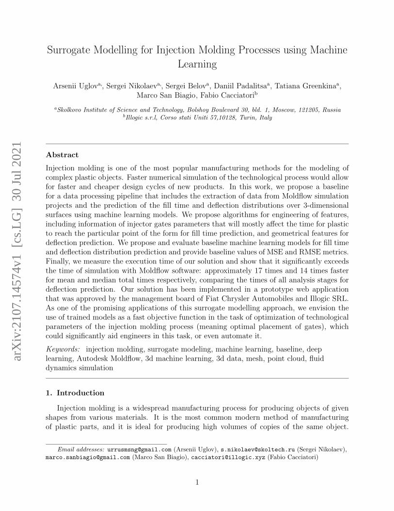
An injection molding machine (Figure 1) consists primarily of two units: a clamping unitand an injection unit. The clamping unit opens and closes the die and maintains the holdingpressure. The injection unit melts plastic pellets and creates melted plastic flow under eithercontrolled speed or pressure (depending on the stage of the process). It consists of a hopper,heaters and a screw which propels the plastic flow. Speed and pressure are controlled by therotation speed of the screw.

The mold is usually a steel cube split into two halves with cavities in the shape of theproduct and auxiliary cavities for plastic canals and a cooling system.

A typical process of injection molding consists of the following steps:

1. Clamping: closing the halves of the mold

2. Injection: introduction of melted polymer flow into the cavity

3. Dwelling: equalizing of polymer pressure through the whole cavity

4. Cooling

2

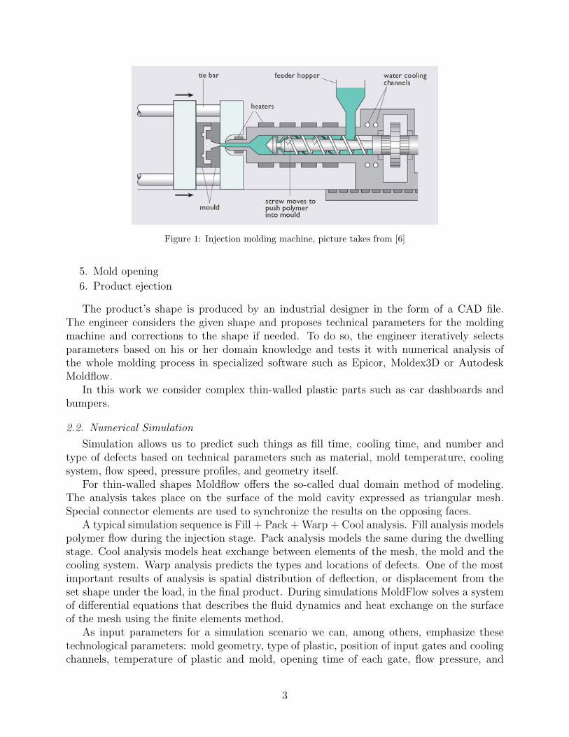
Figure 1: Injection molding machine, picture takes from [6]

5. Mold opening

6. Product ejection

The product’s shape is produced by an industrial designer in the form of a CAD file.The engineer considers the given shape and proposes technical parameters for the moldingmachine and corrections to the shape if needed. To do so, the engineer iteratively selectsparameters based on his or her domain knowledge and tests it with numerical analysis ofthe whole molding process in specialized software such as Epicor, Moldex3D or AutodeskMoldflow.

In this work we consider complex thin-walled plastic parts such as car dashboards andbumpers.

2.2. Numerical Simulation

Simulation allows us to predict such things as fill time, cooling time, and number andtype of defects based on technical parameters such as material, mold temperature, coolingsystem, flow speed, pressure profiles, and geometry itself.

For thin-walled shapes Moldflow offers the so-called dual domain method of modeling.The analysis takes place on the surface of the mold cavity expressed as triangular mesh.Special connector elements are used to synchronize the results on the opposing faces.

A typical simulation sequence is Fill + Pack + Warp + Cool analysis. Fill analysis modelspolymer flow during the injection stage. Pack analysis models the same during the dwellingstage. Cool analysis models heat exchange between elements of the mesh, the mold and thecooling system. Warp analysis predicts the types and locations of defects. One of the mostimportant results of analysis is spatial distribution of deflection, or displacement from theset shape under the load, in the final product. During simulations MoldFlow solves a systemof differential equations that describes the fluid dynamics and heat exchange on the surfaceof the mesh using the finite elements method.

As input parameters for a simulation scenario we can, among others, emphasize thesetechnological parameters: mold geometry, type of plastic, position of input gates and coolingchannels, temperature of plastic and mold, opening time of each gate, flow pressure, and

3

clamping pressure. The results of simulation are spatial distribution of fill time for Fillanalysis, cooling time for Cool analysis, and weld lines and deflection for Warp analysis.Figure 2 shows an example of output of the fill time simulation for a generic dashboardmodel.

Figure 2: Moldflow prediction of fill time for generic car dashboard. Image is taken from an open informationsource [7]

3. Related Works

Here we review the most common approaches that apply machine learning models to three-dimensional objects. Most models can be distinctively categorized by used representation of3D objects.

3.1. Meshed Representation

Meshes discretize an object’s surface with a set of flat polygons, usually triangles. It isthe most common representation in computer graphics and CADs.

The simplest approach to deal with the mesh would be to treat it as a graph and encodegeometrical properties into vertex and edge signals. The two main approaches to construct-ing graph convolutions are based on spectral filtering or local filtering. Depending on thetype of specter approximation or type of local filters, different operations can be derived.Nonetheless, most models allow general representation in terms of a message passing to anode from its neighborhood.

Graph networks are usually isotropic in terms of mutual orientation of nodes and areinvariant under permutations of the neighborhood, but mutual orientation of nodes in a mesh

4

is crucial to defining that mesh. Convolutional operators should thus be anisotropic in termsof orientation between the target and source nodes. However, any definition of orientationvia angle would arbitrarily depend on the choice of reference angle. We thus either need tofix canonical orientation in the node neighborhood for all meshes, as it is done in the case ofimage convolutions on a regular grid. In [8], the authors consider similarly meshed surfacesand introduce fixed serialization of the neighborhood by spiral trajectory from the target; theauthors of [9] use an attention mechanism for soft assignment of neighbors to kernel weightmaps.

As stated by Bernstein et al. in [10], the success of convolution on regular data is basedon implicitly exploited global symmetries of Euclidean spaces. 2-d convolutions, for example,are naturally shift equivariant. A general manifold, and meshes in particular, lacks globalsymmetries that can be exploited, but one can define some locally equivariant operations.Cohen et al. in [11] and [12] introduce a specific type of features on node tangent space andderive gauge equivariant convolution.

3.2. Point Cloud Representation

In this approach, a 3D object expressed as a set of points in a 3D space sampled from thevolume of the object or from the nodes of 3d mesh polygons. It is usually produced by a 3Dsensing method such LiDAR scanners or stereo reconstruction. One of the first successful DLmodels for point clouds was PointNet from [13], where the same (weights sharing) network isapplied to features of each point, and then aggregated by a permutation invariant operator toproduce embedding of a whole cloud. Such an approach cannot grasp the local geometry ofan object’s surface. In [14] Qi et al. proposed clustering a point cloud and applying PointNetto each cluster, resulting in new point cloud, which is processed in same fashion until thewhole point cloud does not merge.

In [15], the authors dynamically built a k-Nearest Neighbors graph in the feature space ofeach layer and then applied a graph convolutional network to obtain new features, repeatingthis process until the desired depth was reached.

Although point cloud models are simpler and can be implemented more easily than meshedmodels, one of their main drawbacks is that they cannot differentiate between points thatare close in 3D space and far in terms of geodesic distance (distance on the surface of theshape).

3.3. Rasterized representation

The most common regular approach is to build voxel representation. The object andbounding space around it are divided into a three-dimensional grid of voxels. Such repre-sentation allows for trivial extension of 2D convolutions [16, 17]. However, complexity andmemory consumption for such an approach grows cubically with resolution. Effective datastructure allows for better time and memory complexity. In [18], Wang et al. split boundingspace recursively in octets of smaller cubes, and use an oct-tree as an effective storage. Thenconvolutions act on neighboring cubes on the same level of the tree, passing aggregated valuesto the coarser level.

Another approach would be in using 2d projections of 3d structures and then applyingtraditional 2d convolutions. There can be single or multiple views projections of a 3d object

5

with additional 2d features, like the distances to the projection plane, and with some mech-anism for aligning predictions from different projections [19]. Such an approach then allowsuse of state-of-the-art 2d convolutional architectures for processing of obtained regular 2drepresentations. And the models used in practice are relatively simple for implementationand training, and they are cost-effective in inference.

It is not quite obvious which of these representations is better suited for our task. In thispaper we present the results for 2d projection representation as a baseline.

4. Our Approach

4.1. Data extraction

The data for further analysis were extracted from Moldflow simulations projects. For thispurpose we export simulation data from Moldflow and then, using developed data loaderscripts, we extract valuable data from an exported set of files for a particular simulation,preprocess it, and pack the aggregated data for all simulations in the Pandas dataframe. Foreach simulation we use the following files to extract data from:

1. a .pat file that contains mesh data. We collect nodes ids, their coordinates and infor-mation for polygons as nodes ids triplets.

2. a .txt file that contains a Moldflow log file. From this file we extract values of technolog-ical parameters (such as Melt temperature, Cooling time, Duration, Filling pressure,Ambient temperature, Mold temperature, Time at the end of filling), and injectiongates information (node ids and Opening time).

3. an .xml file that contains Moldflow simulation results.

Also during the loading process we calculate the shortest paths from nodes to gatesconsidering polygonal mesh as a graph of nodes and edges weighted by the length of theedges. The shortest paths between all nodes and all gates then are calculated according toDijkstra’s algorithm.

4.2. Data processing pipeline

The general scheme of our pipeline for the analysis of extracted data is shown on Fig.3. This diagram shows the general pipeline idea without any actual result distribution ora 3d geometry from our dataset, since we can’t show these details due to non-disclosureagreement.

The pipeline has the following sequential steps:

1. Pre-process point cloud data

2. Extract features for gates

3. Train the Gradient boosting model to predict fill time

4. Generate 2d feature maps from the 3d model with values

5. Train a CNN model to predict deflection distribution in 2d space

6. Reproject 2d deflection distribution back over the 3d mesh

6

Figure 3: The general scheme of data processing pipeline

4.3. Point cloud pre-processing

At first the subset of points of a given size is randomly selected from the model. We takeof about 1/8 of the total points count.

For each of the selected points we then take k nearest points for the area that will beused for smoothing the prediction results. In our experiments we take k=100.

4.4. Extraction of features of gates

For each point we construct an N-dimensional vector of features of gates that will be usedto predict fill time value. Since fill time value is dependent on the distance a plastic shouldtravel to reach a particular place, in our experiments for each point we construct featuresfrom the three nearest gates, which will mostly affect the time of the plastic to reach thispoint. That gives us an 8-dimensional feature vector.

As a first set of values, we take distances to the three nearest gates, calculated as describedin section 4.1.

As a second triplet of features for each of the three selected gates we use its opening timevalue.

Finally, we calculate the three-dimensional vectors of orientation of each selected gaterelatively to each point and then take the values of cos(α1), cos(α2), as the two last features,where α1 and α2 are the angles between the orientation vectors of the first and second andthe first and third gates, respectively.

4.5. Fill time prediction with the Gradient boosting model

Using derived feature vectors for points, we trained the Gradient boosting model to predictthe fill time value. The ground truth distribution of values for this parameter is taken fromthe data, exported from Moldflow simulations.

The prediction is performed for a subset of previously randomly selected points. Then foreach selected point the predicted value is copied over a selected neighboring area. Values for

7

overlapping parts of areas are averaged. This allows us to create smooth distribution thatreflects the continuous nature of the fill time value and reduces computational time.

4.6. Fill time projection to 2d space

For deflection prediction, we project a 3d point-cloud with the predicted fill time distri-bution to the 2d plane. The projection plane is selected so that it minimizes the squaredEuclidean 2-norm for the original and projected points. The projected image is 384x768pixels in size. As a feature map for the second channel, we also obtain a 2d map of a maskthat represents the silhouette of the projection of the mesh, to help the model to distinguishthe projection from the background. This approach allows us to take into account the geo-metrical features of the mesh alongside derivative features of the injector’s gates in the formof predicted fill time.

4.7. Deflection prediction with the CNN model

For the prediction of the distribution of deflection values over the 2d image we use a con-volution neural network model based on the U-Net model [20]. The details of the architectureof the model are described in the appendix.

As a result of inference with our model, we obtain a 2d map of predicted distribution12x24 in size. This 2d representation is then up-scaled, with interpolation, to represent the2d image, 384x768 in size, of predicted deflection distribution over the initial 2d projection.Prediction of 2d deflection map in a lower resolution and then up-scaling it allows us toobtain a smooth result distribution that reflects the continuous nature of the deflection.

4.8. Inflate 2d prediction data back to 3d mesh

The predicted 2d deflection map then is re-projected back onto 3d space to producedistribution over the initial point cloud. For each of 3d points, we pick up the correspondingvalue from the 2d plane using information about 3d-to-2d points correspondence saved onthe projection step.

5. Experiments and Results

5.1. Dataset

We use the dataset obtained from our aforementioned partner, which consists, after ex-traction (described in section 4.1), of 158 Moldflow injection molding simulations for cardashboards and bumpers. Each simulation consists of 3d mesh along with Moldflow simu-lation parameters and results. All simulations are performed using same type of polymer,without a cooling system. Statistics of mesh parameters from the dataset are shown in Table1.

Table 1: Statistics of mesh characteristics

Parameter Min Median MaxVertices 35311 77846 110126Edges 212172 462420 662472Faces 70724 156140 220824

8

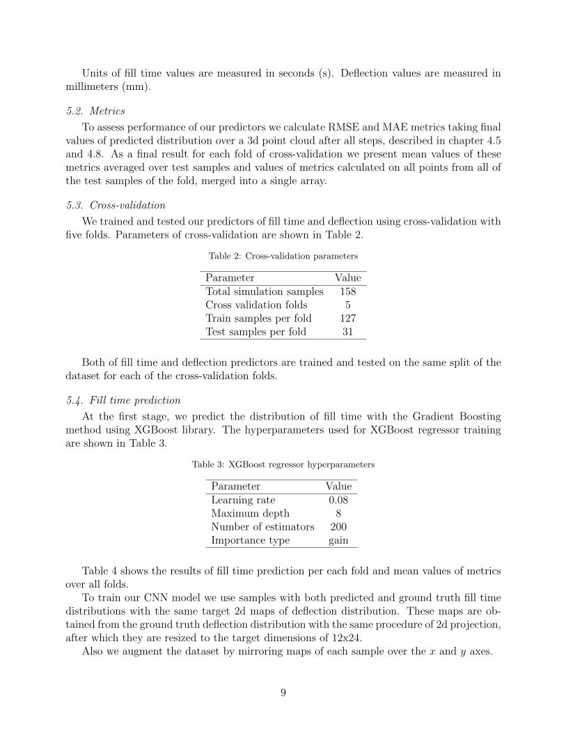
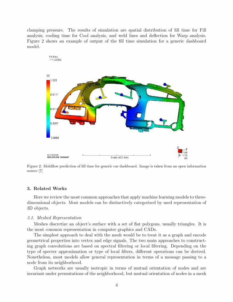
Units of fill time values are measured in seconds (s). Deflection values are measured inmillimeters (mm).

5.2. Metrics

To assess performance of our predictors we calculate RMSE and MAE metrics taking finalvalues of predicted distribution over a 3d point cloud after all steps, described in chapter 4.5and 4.8. As a final result for each fold of cross-validation we present mean values of thesemetrics averaged over test samples and values of metrics calculated on all points from all ofthe test samples of the fold, merged into a single array.

5.3. Cross-validation

We trained and tested our predictors of fill time and deflection using cross-validation withfive folds. Parameters of cross-validation are shown in Table 2.

Table 2: Cross-validation parameters

Parameter ValueTotal simulation samples 158Cross validation folds 5Train samples per fold 127Test samples per fold 31

Both of fill time and deflection predictors are trained and tested on the same split of thedataset for each of the cross-validation folds.

5.4. Fill time prediction

At the first stage, we predict the distribution of fill time with the Gradient Boostingmethod using XGBoost library. The hyperparameters used for XGBoost regressor trainingare shown in Table 3.

Table 3: XGBoost regressor hyperparameters

Parameter ValueLearning rate 0.08Maximum depth 8Number of estimators 200Importance type gain

Table 4 shows the results of fill time prediction per each fold and mean values of metricsover all folds.

To train our CNN model we use samples with both predicted and ground truth fill timedistributions with the same target 2d maps of deflection distribution. These maps are ob-tained from the ground truth deflection distribution with the same procedure of 2d projection,after which they are resized to the target dimensions of 12x24.

Also we augment the dataset by mirroring maps of each sample over the x and y axes.

9

Table 4: Fill time prediction results

FoldRMSEsamples

MAEsamples

RMSEpoints

MAEpoints

#1 0.7600 0.5831 0.8490 0.5234#2 0.5397 0.3840 0.6035 0.3781#3 0.6045 0.4571 0.6561 0.3897#4 0.5243 0.3762 0.5811 0.3597#5 0.6291 0.4698 0.7699 0.4543

SummaryMean 0.6115 0.4540 0.6919 0.4210

To test the deflection predictor we use the predicted fill time for the test sample and takeaverage of four predicted 2d deflection maps for one original and three mirrored 2d fill timemaps. After that we perform the reprojection of the results of 2d deflection prediction backto the 3d point cloud, as described above, and calculate the metrics for this resulting 3ddistribution. Table 5 shows the results of deflection prediction.

Table 5: Deflection prediction results

FoldRMSEsamples

MAEsamples

RMSEpoints

MAEpoints

#1 2.3837 2.0582 2.6504 1.9954#2 1.6406 1.2530 1.9034 1.2312#3 1.1052 0.8111 1.2956 0.7779#4 1.2364 0.8587 1.3846 0.8651#5 3.1082 2.7538 3.2924 2.6459

SummaryMean 1.8948 1.5469 2.1053 1.5031

5.5. Simulation time comparison

We obtained the execution times for each phase of a simulation using our solution. Theconfiguration of the test system is presented in Table 6.

Table 6: Test bench setup

CPU Intel Xeon E5-2630 v4 40 cores 2.20GHzRAM 125.8 GBOS Ubuntu 16.04 LTSGPU GeForce RTX 2080 Ti

We measured time for three main parts of the calculations: initial data pre-processing,fill time prediction and deflection prediction. The summary results are shown in Table 7

For comparison with Moldflow performance we use execution time from log files fromour dataset of simulations. Since these files provide only overall time for the Warp Analysis

10

Table 7: Summary of simulation time with our solution, in seconds

Stage Min Mean Max Std MedPre-processing 13.611 95.961 224.120 66.317 76.022Fill time 1.390 3.529 5.716 1.18 3.534Deflection 1.015 2.294 4.566 0.61 2.302Total 16.016 101.784 232.341 67.873 81.948

phase and for Fill Analysis combined with other types of analysis (for example, with bothPack Analysis and Residual Stress Analysis), if they are provided, we cannot perform directcomparison of times of isolated fill time and deflection prediction. Therefore, for the filltime phase only, we took only simulations that have execution time of Fill Analysis withoutconjunction with any other type of analysis. In our dataset Moldflow simulations wereperformed on different hardware, so to make the comparison more precise, we took onlythose simulations that were performed on a hardware configuration as close to ours as wecould select (CPU of 40 and more cores).

There were seven such simulations in our dataset. The result is shown in Table 8.

Table 8: Execution time for Moldflow simulations with Fill analysis only, in seconds

Min Mean Max291 869.143 1103

It is evident that our solution is faster in passing all the stages that are needed to computefill time distribution, even if we compare the fastest Moldflow simulation, with an executiontime of 291 sec., with the slowest pre-processing and fill time prediction stages with oursolution, which is 229.135 sec.

For deflection prediction time we took simulations that contain a Warp analysis stageand were performed on the most similar hardware. There were 99 simulations selected. Thenfor each simulation we obtained the total time of execution of all stages of the simulation,including analysis stages preceding the Warp analysis (for example, the Fill analysis). Table9 shows the summary of the obtained time periods.

Table 9: Total execution time summary for Warp analysis in selected Moldflow simulations, in seconds

Min Mean Max Std 25% Med 75%127 1765.4 38116 4222.6 520 1161 1594.5

We compare these results with the total time of all stages to obtain deflection predictionwith our solution. There are only nine Moldflow simulations, with a maximum executiontime of 177 sec. and a minimum of 127 sec., that are faster than the maximum total timewith our solution. These Moldflow simulations are with different technological parametersand the same geometry. And our solution gives execution time for these simulations in theinterval from 29.075 to 33.05 sec., which is still multiple times faster.

On average our solution for deflection prediction appeared to be 1663.616 sec. and 17.34(14.17 by median) times faster than Moldflow.

11

Conclusion

In this work we proposed the baseline pipeline for data processing of injection moldingsimulation parameters to predict target distributions of deflection and fill time over a 3dmesh using a surrogate modelling approach. The pipeline includes the extraction of datafrom Moldflow simulation projects and the prediction of the target distributions.

We described how and where to get valuable data from files of injection molding simula-tion, extracted from Moldflow.

Then we proposed the algorithm for engineering of features, that will be used to trainmodel for prediction of fill time distribution. Derived features include information aboutlocation and direction of injector’s gates that will mostly affect the time of plastic to reachthe particular point of a 3d mesh, relative to each point of the point cloud of a mesh, alongsideinformation about the opening time of gates.

As a model for fill time prediction we proposed using the Gradient boosting technique, andwe showed its performance on our data using a five-fold cross-validation check and obtainedthe baseline values of MSE and RMSE metrics for the fill time distribution prediction.

Then we described the algorithm for engineering of features for predicting the deflectiondistribution that will include information about the geometry as well as parameters of gatesin form of predicted fill time distribution.

For the deflection distribution we proposed a 2d convolutional neural network modeland steps for features and target distibution projection to 2d dimensional space and back.We showed the performance of the proposed method using the same cross-validation splitand obtained the baseline values of MSE and RMSE metrics for the deflection distributionprediction.

Finally we measured the execution time of our solution for the steps of targets predictionand compared it to the time of simulations with Moldflow software. The result shows thatour solution significantly excels the Moldflow in execution time: for about 17 times fastercomparing mean and for about 14 times comparing median for total time of all stages ofthe deflection prediction. The slowest fill time prediction with our solution is faster than thequickest with Moldflow. And our slowest deflection prediction is faster than the vast majorityof Moldflow simulations with Warp analysis from our dataset, while for each individualsimulation with our solution is still multiple times faster.

To demonstrate the potential of the described solution, we developed a web applicationprototype that allows a user to upload molding data of a 3d mesh, set up injector’s gatesparameters, perform simulation using our data preprocessing algorithms and trained MLmodels, and obtain vivid visualization of its result. This prototype was presented and ap-proved by the management board of the Fiat Chrysler Automobiles, the Italian automotivemanufacturer.

In the further work, we will aim to improve the quality of the model by the engineeringof more features from the available data and testing the applicability of geometrical modelsfor our task. We will also train our models on more data as it becomes available.

One of the nearest ways of improvement of our current model, we see using a multipleview approach and including information of distance from 3d point to its projection as anadditional geometrical feature. Another direction of model enhancement is to use ANNmodels that work directly with Point Cloud and Mesh or Graph representations, such as

12

DGCNN [15].Finally, we see one of the possible but promising applications of such surrogate modelling

approach in using trained models as a fast objective function in the task of optimizationof technological parameters (i.e. optimal gates placement), which could significantly helpengineers in this task, or even automate it.

Acknowledgements

We thank Vadim Leshchev1 for his great contributions to the preparation of results pre-sentation and technical implementation of ideas of this work, programming tools, and MVPapplication. We thank Ilnur Nuriakhmetov1 for his great help in technical support of thisproject. We also thank Anna Nikolaeva1 for her great help in the scientific research andthe scientific report preparation. We thank Roman Misiutin for his great help in scientificresearch into graph models and this paper preparation.

References

[1] Z.-H. Han, K.-S. Zhang, Surrogate-Based Optimization, in: Real-World Applications ofGenetic Algorithms, InTech, 2012. doi:10.5772/36125.URL www.intechopen.com

[2] F. Ratnikov, Generative Adversarial Networks for LHCb Fast Simulation,arXiv:2003.09762 [hep-ex, physics:physics] (Mar. 2020).

[3] F. Ratnikov, Using machine learning to speed up and improve calorimeter R&D, J. Inst.15 (05) (2020) C05032–C05032, publisher: IOP Publishing. doi:10.1088/1748-0221/

15/05/C05032.

[4] B. Moseley, A. Markham, T. Nissen-Meyer, Fast approximate simulation of seismic waveswith deep learning, arXiv:1807.06873 [physics] (Jul. 2018).

[5] R. Orihara, R. Narasaki, Y. Yoshinaga, Y. Morioka, Y. Kokojima, Approximation ofTime-Consuming Simulation Based on Generative Adversarial Network, in: 2018 IEEE42nd Annual Computer Software and Applications Conference (COMPSAC), Vol. 02,2018, pp. 171–176, iSSN: 0730-3157. doi:10.1109/COMPSAC.2018.10223.

[6] Hot runner mould injection manufacturers, www.anole-hot-runner.com/

hot-runner-mould.htm, accessed: 2021-05-25.

[7] Homepage of element muhendislik, https://www.elementmuhendislik.com/, accessed:2021-05-25.

[8] S. Gong, L. Chen, M. Bronstein, S. Zafeiriou, SpiralNet++: A Fast and Highly EfficientMesh Convolution Operator, 2019.

1Skolkovo Institute of Science and Technology, Moscow, Russia

13

[9] N. Verma, E. Boyer, J. Verbeek, FeaStNet: Feature-Steered Graph Convolutions for 3DShape Analysis, arXiv:1706.05206 [cs] (Mar. 2018).

[10] M. M. Bronstein, J. Bruna, Y. LeCun, A. Szlam, P. Vandergheynst, Geometric deeplearning: going beyond Euclidean data, IEEE Signal Process. Mag. 34 (4) (2017) 18–42.doi:10.1109/MSP.2017.2693418.

[11] P. de Haan, M. Weiler, T. Cohen, M. Welling, Gauge Equivariant Mesh CNNs:Anisotropic convolutions on geometric graphs, arXiv:2003.05425 [cs, stat] (Mar. 2020).URL http://arxiv.org/abs/2003.05425

[12] T. S. Cohen, M. Weiler, B. Kicanaoglu, M. Welling, Gauge Equivariant ConvolutionalNetworks and the Icosahedral CNN, arXiv:1902.04615 [cs, stat] (May 2019).

[13] A. Garcia-Garcia, F. Gomez-Donoso, J. Rodrıguez, S. Orts, M. Cazorla, J. Azorin-Lopez,PointNet: A 3D Convolutional Neural Network for real-time object class recognition,2016, pp. 1578–1584. doi:10.1109/IJCNN.2016.7727386.

[14] C. R. Qi, L. Yi, H. Su, L. J. Guibas, PointNet++: Deep Hierarchical Feature Learningon Point Sets in a Metric Space, arXiv:1706.02413 [cs] (Jun. 2017).

[15] Y. Wang, Y. Sun, Z. Liu, S. E. Sarma, M. M. Bronstein, J. M. Solomon, Dynamic GraphCNN for Learning on Point Clouds, arXiv:1801.07829 [cs] (Jun. 2019).

[16] Z. Wu, S. Song, A. Khosla, F. Yu, L. Zhang, X. Tang, J. Xiao, 3D ShapeNets: A DeepRepresentation for Volumetric Shapes, arXiv:1406.5670 [cs] (Apr. 2015).

[17] D. Maturana, S. Scherer, VoxNet: A 3D Convolutional Neural Network for real-timeobject recognition, in: 2015 IEEE/RSJ International Conference on Intelligent Robotsand Systems (IROS), IEEE, Hamburg, Germany, 2015, pp. 922–928. doi:10.1109/

IROS.2015.7353481.

[18] P.-S. Wang, Y. Liu, Y.-X. Guo, C.-Y. Sun, X. Tong, O-CNN: Octree-based ConvolutionalNeural Networks for 3D Shape Analysis, ACM Trans. Graph. 36 (4) (Jul. 2017). doi:

10.1145/3072959.3073608.

[19] H. Su, S. Maji, E. Kalogerakis, E. Learned-Miller, Multi-view convolutional neural net-works for 3d shape recognition, in: Proceedings of the IEEE international conference oncomputer vision, 2015, pp. 945–953.

[20] O. Ronneberger, P. Fischer, T. Brox, U-net: Convolutional networks for biomedicalimage segmentation (2015). arXiv:1505.04597.

14

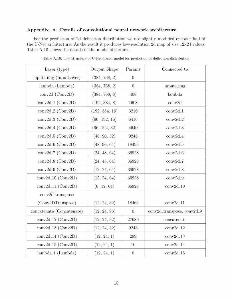
Appendix A. Details of convolutional neural network architecture

For the prediction of 2d deflection distribution we use slightly modified encoder half ofthe U-Net architecture. As the result it produces low-resolution 2d map of size 12x24 values.Table A.10 shows the details of the model structure.

Table A.10: The structure of U-Net-based model for prediction of deflection distribution

Layer (type) Output Shape Params Connected to

inputs img (InputLayer) (384, 768, 2) 0

lambda (Lambda) (384, 768, 2) 0 inputs img

conv2d (Conv2D) (384, 768, 8) 408 lambda

conv2d 1 (Conv2D) (192, 384, 8) 1608 conv2d

conv2d 2 (Conv2D) (192, 384, 16) 3216 conv2d 1

conv2d 3 (Conv2D) (96, 192, 16) 6416 conv2d 2

conv2d 4 (Conv2D) (96, 192, 32) 4640 conv2d 3

conv2d 5 (Conv2D) (48, 96, 32) 9248 conv2d 4

conv2d 6 (Conv2D) (48, 96, 64) 18496 conv2d 5

conv2d 7 (Conv2D) (24, 48, 64) 36928 conv2d 6

conv2d 8 (Conv2D) (24, 48, 64) 36928 conv2d 7

conv2d 9 (Conv2D) (12, 24, 64) 36928 conv2d 8

conv2d 10 (Conv2D) (12, 24, 64) 36928 conv2d 9

conv2d 11 (Conv2D) (6, 12, 64) 36928 conv2d 10

conv2d transpose

(Conv2DTranspose) (12, 24, 32) 18464 conv2d 11

concatenate (Concatenate) (12, 24, 96) 0 conv2d transpose, conv2d 9

conv2d 12 (Conv2D) (12, 24, 32) 27680 concatenate

conv2d 13 (Conv2D) (12, 24, 32) 9248 conv2d 12

conv2d 14 (Conv2D) (12, 24, 1) 289 conv2d 13

conv2d 15 (Conv2D) (12, 24, 1) 10 conv2d 14

lambda 1 (Lambda) (12, 24, 1) 0 conv2d 15

15