Surface modeling topsoil distribution on a reclaimed coal-mine site at Blackmesa Mine Complex, Kayenta, Arizona

Janine Ferarese

University of Denver Department of Geography

Capstone Project

for

Master of Science in Geographic Information Science

October 31, 2011

Ferarese-ii

Abstract

A necessary precursor to ensure proper vegetation growth on reclaimed

coal-mine areas is even distribution of topsoil. This capstone discusses

development of surface models to describe the accurate determination and

visualization of the distribution of topsoil. Prediction surfaces from topsoil-

depth point samples were created using the surface interpolation methods,

Inverse Distance Weighted and Kriging. The validity and accuracy of each

method was assessed to determine the best method to evaluate actual

topsoil distribution at a coal mining site. The model can be utilized by non-

spatially trained personnel working in the mining arena as an aid in

assessing how appropriately the topsoil has been distributed over newly

reclaimed mine areas.

Ferarese-iii

Table of Contents

Abstract .............................................................................................. ii

Table of Contents ................................................................................ iii

List of Figures ..................................................................................... iv

Introduction ......................................................................................... 2

Background ......................................................................................... 4

Thesis Statement ................................................................................. 7

Literature Review ................................................................................. 9

General Discussion on Spatial Modeling ................................................. 13

Methodology ...................................................................................... 30

Results .............................................................................................. 45

Conclusion ......................................................................................... 51

Future Opportunities ........................................................................... 52

References ........................................................................................ 54

Appendix A – List of Acronyms ............................................................. 56

Appendix B – IDW Model Parameters .................................................... 57

Appendix C – Kriging Model Parameters ................................................ 58

Ferarese-iv

List of Figures

Figure 1. Reclamation Specialists Monitoring Topsoil-Depth. Courtesy OSM. . 8

Figure 2. The Normal Distribution. Graphic from Wikipedia (Mwtoews.) ..... 17

Figure 3. QQ Plot. Graphic from Wikipedia (Skbkedas.) ........................... 19

Figure 4. Boxplot To Normal Probability Function. Graphic from Wikipedia (Jhguch.) ..................................................................................... 20

Figure 5. Voronoi Cluster Map Example. ................................................ 23

Figure 6. Voronoi Entropy Map Example. ............................................... 24

Figure 7. Polynomial Trend Example. .................................................... 25

Figure 8. General Semivariogram. Graphic from Wikipedia. ...................... 28

Figure 9. Blackmesa Mine Complex Area of Interest Map. ........................ 31

Figure 10. Spatial Statistics of Sampled Points. ...................................... 33

Figure 11. Geostatistical Modeling Summary Flowchart............................ 34

Figure 12. Boxplot of Topsoil-depth....................................................... 35

Figure 13. Histogram and QQ Plot of Raw Data Values. ........................... 36

Figure 14. Voronoi Cluster Map of Topsoil-depth. .................................... 37

Figure 15. Examination of Potential Outlier. ........................................... 38

Figure 16. Rational for Not Excluding Potential Outlier. ............................ 39

Figure 17. Voronoi Entropy Map of Topsoil-depth. ................................... 40

Figure 18. Trend Analysis of topsoil-depth. ............................................ 41

Figure 19. Voronoi Standard Deviation Map of Topsoil-depth. ................... 42

Figure 20. Semivariogram of Topsoil-depth. ........................................... 44

Figure 21. IDW and Simple Kriging Prediction Surfaces. .......................... 46

Figure 22. Standard Error of Prediction Surface for the Kriging Derived Prediction Surface. ........................................................................ 47

Figure 23. Probability Surface of 24-inch Minimum Requirement. .............. 49

Figure 24. Cross-validation Statistics for IDW and Simple Kriging Comparison. ................................................................................. 50

Ferarese-2

Introduction

Coal is a combustible rock that contains more than 50 percent by

weight carbonaceous material. The precursor to coal is peat; the

unconsolidated deposit of large amounts of plant remains which have

accumulated in widespread wetland environments such as bogs and

swamps. Over long periods of time (millions of years) deeply buried peat is

transformed physically and chemically into coal via extreme heat and

pressure from overlying sediments.

Coal contains an abundant amount of carbon and when carbon, a

naturally occurring element in living matter, combines with hydrogen a

compound called a hydrocarbon is produced. Such natural hydrocarbons,

including coal, are referred to as fossil fuels because they originate from the

accumulation and transformation of plants and in some cases, other

organisms.

Fossil fuels are burned to produce heat which in turn can be used to

produce electricity. Coal is the most abundant fossil fuel on earth and the

most dominate fuel for producing electricity. In the United States, coal is the

leading energy resource, accounting for almost one third of the country’s

total energy production and more than 51% of the nation’s electrical power

production. (Greb et al, 2006).

As our most abundant domestic source of energy, coal fills an essential

part of the nation’s energy needs. Unfortunately, coal production is linked

Ferarese-3

with adverse environmental issues and concerns particularly related to

disturbance of hydrologic systems, ground subsidence, and post-mining land

use. In addition, mitigating the effects of past mining practices, and

increasing the health of and decreasing safety risks to the public pose

difficult challenges for government’s regulatory control.

Beginning in the 1740’s, commercial coal mining has been occurring

in the United States without regard to environmental consequences.

Prompted by major environmental impacts from coal mining during the

1960’s and 1970’s, the U.S. Congress enacted The Surface Mining Control

and Reclamation Act (SMCRA) in 1977. These federal laws and regulations

define minimum requirements for the performance of specific activities

during the mining operation and have set standards for environmental

protection that must be met. The SMCRA defined minimum standards to

ensure that the lands affected by coal mining operations are returned to

productive use.

The Office of Surface Mining Reclamation and Enforcement (OSM), a

bureau under the U.S. Department of Interior, is charged with carrying out

the requirements of SMCRA.

OSM carries out the requirements of SMCRA in cooperation with States

and Indian tribes. OSM's objectives are to “ensure that coal mining activities

are conducted in a manner that protects citizens and the environment during

mining, to ensure that the land is restored to beneficial use after mining,

Ferarese-4

and to mitigate the effects of past mining by aggressively pursuing

reclamation of abandoned coal mines.” 1

Background

In adherence with the rules of SMCRA, prior to the start of coal mining

activities, a permit must be obtained from the OSM. The permit application

must describe several requirements: (1) the existing conditions at the

proposed mine site, (2) the procedures and equipment to be used in the

operation, (3) the potential environmental impacts resulting from the

operation, (4) the measures to be taken to protect the environment, (5) the

intended post-mining land use to which the area will be returned upon

completion of mining, and (6) the specific techniques to be used to reclaim

the area to the intended use. The process includes restoring the land to its

approximate original appearance by restoring topsoil and planting native

vegetation and ground covers. (U.S. Department of Interior, 2007).

Throughout the life of the mine (LOM), i.e. the time frame when earth

is first broken to begin extraction of coal through when final reclamation is

completed, compliance inspections of the progress of reclamation and

observance to regulations of SMCRA are made by the OSM either directly or

via oversight of State or Tribal programs. At each step along the way the

mine operator under the enforcement of OSM must comply with Federal and

State laws and with SMCRA. The LOM can span decades, especially in the 1 OSM Mission Statement from http://www.osmre.gov/aboutus/Mission.shtm

Ferarese-5

exceedingly large coal mine operations in the west, and many regulatory

inspectors and other earth scientists and engineers work in concert over this

time frame.

Reclamation occurs contemporaneously at the mine site in that

reclamation activities will be under way in one area while coal removal

continues nearby. To ensure compliance at each step, an inspection is

conducted monthly for specific areas deemed problematic and one inspection

per quarter to include the entire mine site. Upon completion of the

inspection, a written report is produced for documentation purposes. The

inspection report is an important document that may become a factor if legal

action ensues.

Surface coal mining is more complex than simply uncovering the coal

and removing it. Attention must be paid to environmental concerns,

especially returning the mined land to productive use, and in actuality

surface mining entails a sequence of activities.

Although the characteristics of each mine site, including the geology,

hydrology, and topography will affect the mining method used, the following

activities in sequential order are common to all surface coal mine operations:

(1) erosion and sedimentation control, (2) road construction, (3) clearing

and grubbing, (4) topsoil removal (salvage) and handling, (5) overburden

removal and handling, (6) coal removal and handling, (7) reclamation.

Ferarese-6

The first steps in preparing an area for coal removal is to clear and

grub. Clearing is the act of cutting and/or removing all trees and brush from

an area. Grubbing is removing any remaining roots and stumps, low growing

vegetation, and grass. These are necessary steps to facilitate topsoil

salvage.

Topsoil is the uppermost layer of soil in which plant growth is best

achieved. This layer must be removed and properly stored in order to

enhance soil productivity, as it is desirable to re-lay this same topsoil during

the reclamation phase. However, in areas where the topsoil is of poor quality

or unavailable in sufficient quantities the permit may allow the use of topsoil

substitutes in reclaiming the land. In either case, there are regulations

addressing the redistribution of topsoil. One of which is that topsoil must be

redistributed to a depth specified in the mining permit and in a manner that

achieves an approximate, uniform thickness.

Sound science is the foundation for effectively implementing SMCRA

and use of geospatial technology can be an invaluable tool in the application

of SMCRA towards improving public safety and decreasing detriment to the

environment.

For the greatest part the coal industry has not fully adopted the power

of Geographic Information Systems (GIS). Reliance on antiquated mapping

techniques is less than a best solution to reclamation. “Many in the mining

industry have adopted Computer Aided Design software, which is a step in

Ferarese-7

the right direction, but it is not without its difficulties. The solution is

adoption of modern geospatial standards and techniques.” (Evans, 2008).

Thesis Statement

The aim of this thesis is to describe a process that will create a cell-

based (raster2) analysis prediction surface from sampled topsoil-depth point

values to aid in determining how evenly a mine operator has spread the

required minimum depth of topsoil over newly reclaimed areas on surface

coal mines.

An important objective of the laws enforced by SMCRA is to ensure

that mined lands are returned to productive use. An important precursor to

this end is the necessity that topsoil be evenly distributed and to a specified

depth over the area to be reclaimed. To ensure this requirement is met,

OSM or the affiliated State or Tribal SMCRA regulatory body conducts

compliance inspections of the area.

During a SMCRA inspection, Regulatory Specialists trained in the use

of Global Positioning System (GPS) technology monitor the depth of topsoil

that has been redistributed by collecting soil-depth data using a Topsoil

Probe and portable GPS unit. (Figure 1).

Coordinates of sample locations along with the attribute depth of the

topsoil at that location are downloaded from the GPS receiver and converted

2 A raster is a spatial image where the data is expressed as a matrix of cells or pixels, with spatial position implicit in the ordering of the pixels.

Ferarese-8

into a GIS point feature class or shapefile3. The Reclamation Specialist

visually reviews the shapefile onscreen in a GIS or creates a hard-copy

graphic of the points with their respective topsoil depths annotated in order

to determine areas where minimum topsoil depth has not been achieved or

has been over-placed too thickly.

Figure 1. Reclamation Specialists Monitoring Topsoil-Depth. Courtesy OSM.

This operation has potential to be greatly enhanced to provide greater

interaction of the data among mining professionals and expedite the

timeliness, efficiency, and accuracy in decisions required to be made

following inspection and production of the written inspection report.

SMCRA requires a minimum average top-soil depth evenly distributed

over a reclaimed area. In the absence of more stringent analysis of the

3 A shapefile (referred to as a feature class when implemented in a geodatabase) is digital vector storage format for storing geometric location and associated attribute information.

Ferarese-9

overall distribution of depth the possibility exists that an area could be

deemed to be within requirements by simple virtue of the arithmetic average

of all points sampled over the entirety of the area being within that

minimum average. This does not reflect the spirit of the law and could

provide potential for a greater chance of improper vegetative growth

resulting in subpar reclamation.

It is possible to more accurately determine and visualize the

distribution between measured topsoil depth and the minimum depth called

for in the mining permit. Further, there is need to automate the process to

aid non-spatially trained mining personnel in making assessment.

Literature Review

Several studies related to the wide range of complex problems

associated with coal mine permitting and abandoned mine land problems are

introduced followed by reviews of studies examining surface modeling

applications.

The danger posed by old or poorly designed maps is very real; a

missing map or a map that is incomplete or in error can and has cost human

lives, damage to homes and property, and proven detrimental to the

environment. “A reclamation program needs a systematic, logical process

able to discriminate among many similar project contenders to meet the

needs of SMCRA and to be legally defensible.” (Rohrer, et al, 2008).

Ferarese-10

One facet of the SMCRA rules define the requirement that a

Cumulative Hydrologic Impact Assessment (CHIA) be completed before

proposed coal mine permits may be accepted. West Virginia University

(WVU) with support from OSM developed a suite of software tools to support

CHIA’s of proposed mine activities in West Virginia. Incorporating a GIS

interface, they added the Environmental Protection Agency’s (EPA)

watershed model named “Hydrologic Simulation Program-Fortran” (HSPF) to

their own Watershed Characterization and Modeling System (WCMS) to

predict changes in water-quality and quantity caused by surface mining. The

model contains over 20 parameters and uses a joint calibration approach,

using historical stream flow records from five watersheds and four

verification watersheds throughout West Virginia. (Lamont et al, 2008).

The marriage of GIS and Remote Sensing is one not destined for

separation. “Many GIS practitioners didn’t appreciate the contributions of

remote sensing to GIS in the past and its tremendous potential

contributions.” (Green, 2009). The Pennsylvania Department of

Environmental Protection (PA-DEP) and OSM cooperated on a project that

created 3-dimensional models of large anthracite open-pit mining operations

in Pennsylvania. (Anthracite is the highest ranking form of coal which

produces more heat per ton when burned because it is a more concentrated

form of carbon due to increased time and pressure during the alteration

from peat.)

Ferarese-11

It is necessary to accurately determine the volume of open pits that

result from certain methods of surface coal mining. Accurate estimates of

backfill material are needed to calculate bond liability to the mine operator.

For very large affected areas such as the case in areas in east-central

Pennsylvania the use of remote sensing technology is critical to abate the

cost and difficulties, and simple inability to accurately ground measure such

large areas. Using color high-resolution aerial photographic imagery the PA-

DEP and OSM generated digital photogrammetric data with the goal of three-

dimensionally modeling mine sites for volumetric calculations (Hill, 2004).

Analytical approaches to GIS have evolved over the few decades since

its inception culminating in the science of spatial statistics and spatial

analysis whereby defining geographic relationships leads to solutions that aid

in modeling landscape diversity and pattern. Spatial statistics and analysis

can augment traditional statistics by providing means to map variations in

data by translating discrete point data into a continuous surface representing

the geographic distribution of the data. Many studies have been done using

geostatistical techniques that benefit from the use of interpolation

techniques.

Spatial variability of soil physical properties was carried out using

geostatistical analysis to produce productivity rating systems for use in

precision farming. Rating maps of parameters were prepared as a series of

colored contours using Kriging interpolation and semivariogram models to

Ferarese-12

support findings that good soil physical heath is essential for optimum

sustained crop production (Amirinejad 2011).

In a similar study the relationship between soil organic carbon (SOC)

and landscape aspects in a region of Northeast China was conducted which

explored using geostatistical Kriging interpolation techniques to distinguish

the spatial distribution pattern of SOC (Liu, 2006).

The estimation of spatial variability of precipitation has been shown to

be crucial for accurate distributed hydrologic modeling (Zhang, 2009). The

study by Zhang used a GIS system incorporating Inverse-Distance-

Weighting (IDW) and Kriging as well as other methods to facilitate automatic

spatial precipitation estimation. The study reports that spatial precipitation

maps estimated by different interpolation methods have similar areal mean

precipitation depth but significantly different values of maximum and

minimum precipitation. Zhang suggests implementing multiple spatial

interpolation methods and evaluating their estimates using a correlation

coefficient.

This exemplifies the point that proper use and interpretation of created

surfaces cannot go understated. A common problem in geographic data

analysis is incorrectly creating and interpreting, or failing to interpret,

resultant maps (Wingle, 1992). A study evaluating the accuracy of several

interpolation techniques including IDW and Kriging found that irrespective of

the surface area, few differences existed between the employed techniques

Ferarese-13

if the sampling density was high, but performance tended to vary at lower

sampling densities (Chaplot, et al., 1999). A handicap in representing

surfaces is the existence of noise (Demirhan, 2003) wherein with

environmental investigations noise can be introduced by sampling errors in

the form of duplicate samples taken from the same location resulting in

different observation values.

An interpolated surface can produce an appealing picture, but remain

only that in the absence of proper construction and interpretation. It is

important to be knowledgeable about the uncertainty of the predictions.

Using statistical theory and the functionality of GIS software, the analysis,

modeling, and interpretation of data with location coordinates can be

performed using techniques termed spatial data analysis. Specifically,

continuous data such as that representing topsoil-depth and location use a

spatial analytical technique called geostatistics.

General Discussion on Spatial Modeling

Analysis of data precedes the modeling of it. Analysis must begin with

exploration of the data so that insight is gained towards the proper

application of the methods to be used in the modeling process.

The Environmental Systems Research Institute (ESRI©) ArcGISTM

Desktop extension, Geostatistical Analyst, and the Spatial Statistics toolbox

can be used to aid in analyzing and modeling the distribution of topsoil in

newly reclaimed areas on surface coal mine sites.

Ferarese-14

The ArcGISTM Geostatistical Analyst extension is a collection of tools

used for spatial data exploration and includes the ability to produce

histograms, scatter plots, and semivariograms of the data. Geostatistical

Analyst can be used in the identification of anomalies or outliers in the

dataset as well as serving to help determine the optimal interpolation

prediction method. Additionally, it can be used to create the interpolated

prediction surface, including the prediction uncertainty.

The ArcGISTM Spatial Statistics toolbox contains statistical tools for

analyzing spatial distributions, patterns, processes, and relationships.

Products resulting from utilizing GIS tools are visually appealing and

impressive, and it should be kept in mind that “it is easy to lose sight of

something that everyone knows at some level, namely, that most datasets

have errors both in attributes and in locations, and that processing data

propagates errors.” (Krivoruchko, 2011) Further, the best way to be

confident in the output from a statistical model is to understand the key

ideas behind the model. (Krivoruchko, 2011)

The approach to applying statistical analysis techniques to continuous,

terrestrial geographically based (i.e. location) data is known as geostatistical

analysis or geostatistics. Geographic data do not usually conform to the

requirements of standard statistical procedures due to spatial

autocorrelation.

Ferarese-15

Spatial autocorrelation is the relationship of how a variable correlates

with itself over space. It is the assumption, as stated by Tobler’s First Law of

Geography, that points closer together have smaller differences between

their values than points farther apart from each other. Random patterns do

not exhibit spatial autocorrelation so if there is any systematic pattern in the

spatial distribution of a variable, it is said to be spatially autocorrelated;

measuring the extent to which the occurrence of an event in one area unit

constrains, or makes more probable, the occurrence of an event in a

neighboring area unit. The term is usually applied to ordered datasets where

the correlation depends on the distance and direction separating

occurrences.

Consideration of spatial autocorrelation necessitates the application of

geostatistics in modeling distributed topsoil-depth because it employs

analytical techniques and methods using spatial software including

geographic information systems. The results of geostatistical analysis

typically are primarily derived from observation rather than experimentation

but most advanced techniques require knowledge of the discipline they are

to be applied to as well as professional judgment in their use and

interpretation.

Prior to the start of any spatial analysis and before the actual modeling

of a surface, it is advisable to visually inspect the data by examining its

location and distribution to determine any spatial relationships. The mean or

Ferarese-16

center location can be determined by calculating the average x- and y-

coordinates of the dataset. Because the average value can be affected by

extreme values, comparison of the mean center with the middle, or median

center location, determined by ranking the x- and y-coordinates in numeric

order and choosing the middle value in the list, can yield information on

whether some locations in the data are dispersed or tightly clustered. The

directional distribution of the data lends information about the spread of the

data based upon the standard deviation of the x- and y-coordinate locations.

Equally important is exploration of the data values themselves (in this

case topsoil-depth) for investigation into any variation and trends inherent

within the spatial data. Some geostatistical analysis tools assume the data is

normally distributed and operate correctly only if it is the case.

The Normal distribution is a continuous probability distribution of a

measurement, x, that is subject to a large number of independent, random,

additive errors. Mathematically it is the Gaussian function,

where, μ is simultaneously the mean, median, and mode (i.e. the location of

the center of the peak), σ2 is called the variance and describes how

concentrated the distribution is about the center. The square-root of the

Ferarese-17

variance is the standard deviation, σ, which measures the width of the

density function.

If the data exhibit characteristics of the Normal distribution, then

graphically the distribution is represented by a bell-shaped curve where

there is a clustering of values near the mean. There will be equal numbers

of values on either side of the center of the curve. In Figure 2 each colored

band has a width of one standard deviation. The numbers written as

percentages represent the percent of the dataset accounted for.(e.g. 68.2%

of the set have values within one standard deviation of the mean, 95.4%

have values within two standard deviations, and 99.6% within three

standard deviations.)

Figure 2. The Normal Distribution. Graphic from Wikipedia (Mwtoews.)

Ferarese-18

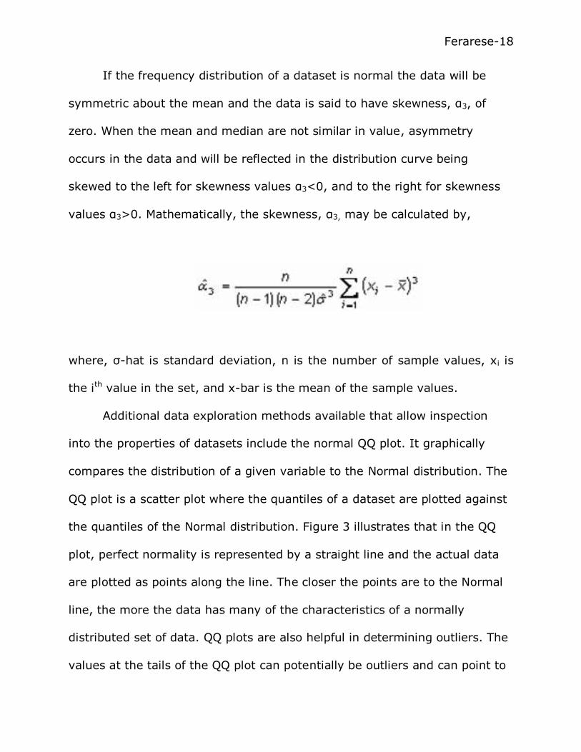
If the frequency distribution of a dataset is normal the data will be

symmetric about the mean and the data is said to have skewness, α3, of

zero. When the mean and median are not similar in value, asymmetry

occurs in the data and will be reflected in the distribution curve being

skewed to the left for skewness values α3<0, and to the right for skewness

values α3>0. Mathematically, the skewness, α3, may be calculated by,

where, σ-hat is standard deviation, n is the number of sample values, xi is

the ith value in the set, and x-bar is the mean of the sample values.

Additional data exploration methods available that allow inspection

into the properties of datasets include the normal QQ plot. It graphically

compares the distribution of a given variable to the Normal distribution. The

QQ plot is a scatter plot where the quantiles of a dataset are plotted against

the quantiles of the Normal distribution. Figure 3 illustrates that in the QQ

plot, perfect normality is represented by a straight line and the actual data

are plotted as points along the line. The closer the points are to the Normal

line, the more the data has many of the characteristics of a normally

distributed set of data. QQ plots are also helpful in determining outliers. The

values at the tails of the QQ plot can potentially be outliers and can point to

Ferarese-19

the necessity to further investigate such points before continuing with an

analysis.

Figure 3. QQ Plot. Graphic from Wikipedia (Skbkedas.)

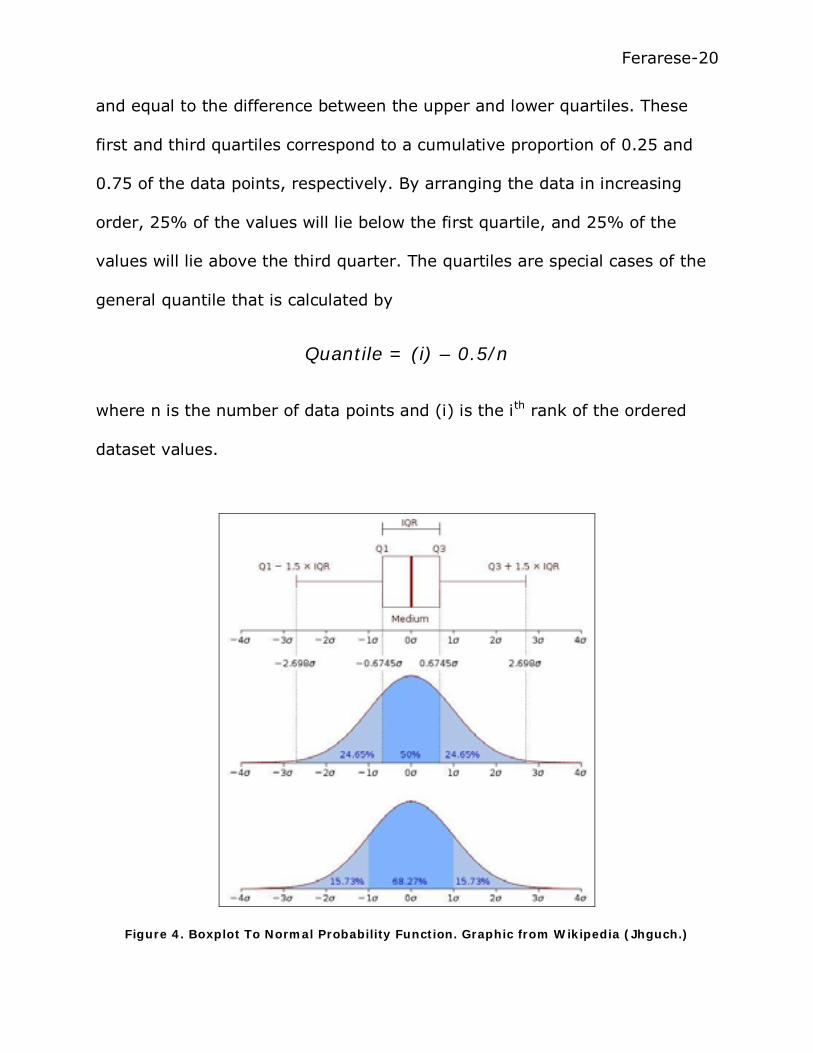
Another quick and convenient descriptive statistical aid to graphically

explore datasets such as topsoil-depth sample points is through use of the

Boxplot, sometimes called the box-and-whisker diagram. A boxplot

summarizes five descriptive statistical parameters: the minimum sample

value, the lower quartile (Q1), the median (Q2), the upper quartile (Q3),

and the maximum sample value. A boxplot generally can also indicate

observations that may be outliers. Figure 4 illustrates the comparison

between the boxplot and the Normal distribution. In Figure 4, IRQ is the

“interquartile range,” being the mid-spread which contain 50% of the data

Ferarese-20

and equal to the difference between the upper and lower quartiles. These

first and third quartiles correspond to a cumulative proportion of 0.25 and

0.75 of the data points, respectively. By arranging the data in increasing

order, 25% of the values will lie below the first quartile, and 25% of the

values will lie above the third quarter. The quartiles are special cases of the

general quantile that is calculated by

Quantile = (i) – 0.5/n

where n is the number of data points and (i) is the ith rank of the ordered

dataset values.

Figure 4. Boxplot To Normal Probability Function. Graphic from Wikipedia (Jhguch.)

Ferarese-21

The “peaked-ness” of a frequency distribution is measured by a

parameter known as kurtosis. Similar to the idea of skewness which is a

measure of the symmetry of a distribution, kurtosis, 4, describes the shape

of the frequency curve; more pointy distributions tend to have higher

kurtosis values. Kurtosis serves to describe the size of the tails of a

distribution, the measure of which can provide the likeliness that the

distribution will produce outliers. Normal distributions will exhibit the value

of 3 for the kurtosis measure. Mathematically, kurtosis can be calculated by

where, σ-hat is standard deviation, n is the number of sample values, xi is

the ith value in the set, x-bar is the mean of the sample values, and

,

It is important in the data exploration phase that it is determined how

the data is distributed, because some Geostatistical Analyst interpolation

tools assume the data is normally distributed. In instances where this is not

the case it may be possible to apply transformations to the data that can

Ferarese-22

sometimes make the datasets more Normal. Data transforms used in

Geostatistical Analyst includes the Box-Cox transformation that is a family of

transforms defined for positive values and described by,

where k is an integer parameter and x is the value being transformed.

If the frequency distribution for a dataset is broadly uni-modal (one

major peak) and left-skewed, the natural log transform (logarithms base e)

can adjust the pattern to make it more symmetric and similar to a Normal

distribution.

The process of ranking the data and then mapping each rank to the

corresponding data rank of a normal distribution is known as the normal

score transformation, another method to help normalize data.

Other exploratory analysis of spatial data includes the geostatistical

methods of Voronoi Mapping and Global Trend Analysis.

A Voronoi map is constructed by forming a series of polygons around

the location of topsoil-depth sample points such that any location within an

individual polygon boundary is closer to the sampled point inside that

polygon than to any other sampled point. Sampled points whose surrounding

polygon shares a border with other sampled points’ polygons will be

considered neighbors, allowing a variety of local statistics to be computed. It

Ferarese-23

is possible to use the ESRI© Geostatistical Analyst extension Voronoi

Mapping tool in a topsoil-depth study to aid in identifying potential local

outliers. The cluster Voronoi method involves placing the data into five class

intervals. If the class interval of a polygon is different from its neighbors the

software colors the polygon grey to distinguish it. Figure 5 illustrates an

example of of a Voronoi Cluster Map where the grey cells reflect potential

outliers.

Figure 5. Voronoi Cluster Map Example.

Stationarity, a property in which the relationship between two points

depends not upon their exact location but only the distance between them,

Ferarese-24

is another assumption of many geostatistical analysis techniques. An entropy

Voronoi map can be used to examine this local variation between data

points. It is calculated based on the class of each surrounding polygon.

Figure 6 illustrates an example of a Voronoi Entropy Map. The red and

orange areas reflect areas with higher variability and are thereby less

stationary than the light greener colors.

Figure 6. Voronoi Entropy Map Example.

If data do not display appropriate stationarity it could be due to a

trend being present in the data. A trend is analyzed by fitting a polynomial

function to describe the variation in the data,

Ferarese-25

where n is a non-negative integer and where each value {an, ..., a0} is a

constant. The order of the polynomial refers to the exponent in the leading

term. A first-order polynomial is linear and displays as a straight line, a

second-order as a parabola, and a third-order as a cubic function.

The ESRI© Geostatistical Analyst extension Trend Analysis tool

provides a three-dimensional perspective of data where sample locations are

plotted on the x,y plane with the height (topsoil-depth value) of the data

projected onto the x,z and y,z planes as scatter plots. Figure 7 illustrates an

example of how a cubic trend (3rd order polynomial) and a weak, parabolic

trend (2nd order) could present. Trend analysis can indicate if there is large-

scale data variation and in what direction; the blue line is North-South, the

green line is East-West.

Figure 7. Polynomial Trend Example.

Ferarese-26

After completion of the exploration of data comes creation of the

interpolated topsoil-depth surface. Interpolation involves the prediction of

values at locations where no sample has been taken and is derived from

functions on the known values at actual sampled locations.

Two of the most common interpolation techniques include Inverse

Distance Weighting (IDW) and the family of methods called Kriging. IDW is a

deterministic method, meaning the interpolation involves non-statistical,

mathematical methods that predict surface cell values for unmeasured x,y

locations using the actual measured topsoil-depth point values surrounding

the unknown, predicted locations. It explicitly implements Tobler’s First Law

of Geography by assuming that each measured topsoil-depth point has a

local influence that diminishes with distance. It weights points closer to the

unknown, predicted x,y location to a greater amount than locations further

away. As the distance approaches zero (i.e. the location of the predicted

point equals that of the measured point) the relative weight approaches 1.

Therefore, IDW is an exact interpolator, meaning the predictions will equal

the measured values at the location of the measured value. That is, the

interpolated surface can never exceed the measured values. A power

function, p, determines the rate at which the weights decrease with distance

from the measured point. As such, the weights are proportional to the

inverse distance between the actual measured point and the unknown,

predicted point raised to the power, p. To determine the optimal p value it is

Ferarese-27

necessary to minimize the root-mean-square predicted error (RMSPE) which

is a summary statistic that quantifies the error of the prediction surface. The

Geostatistical Analyst extension will iteratively calculate different power

values to determine the lowest RMSPE and hence, the optimum power.

While the deterministic technique of IDW uses only the existing

configuration of measured sample points and depends solely on the distance

to the prediction location to create the interpolated surface, the Kriging

methods use geostatistical techniques that incorporate the statistical

properties of the measured sample points. Kriging is a multi-step process

that necessitates exploratory data analysis as described above. Additionally,

because it is based on stochastic principles it can produce error or

uncertainty surfaces along with the prediction surface, as well as surfaces

that define the probability of predicted values exceeding (or failing to exceed

as in the case of minimum topsoil-depth) a critical value. The kriging

method involves quantifying the underlying spatial structure of the data

through a process known as variography. It is an advanced geostatistical

procedure based in fitting models that include autocorrelation.

Autocorrelation is assessed and quantified using a semivariogram

function (gamma) which plots one-half the square of the difference between

two values against the distance separating them.

Ferarese-28

where si and sj are the two points in the pair and Z(s) is the value at each

point. As the distance separating the two points increases so does the

difference between their values increase, if spatial autocorrelation exists.

Figure 8 is an illustration of the general semivariogram plot.

Figure 8. General Semivariogram. Graphic from Wikipedia.

The height of the semivariogram is called the Sill and defines the

variation between pairs of data points. The variation increases with distance

and the Range of the semivariogram is that distance between pairs of points

where the function flattens out; past this point the values are considered

independent and no longer spatially dependent.

Ferarese-29

Underpinning the geostatistical modeling technique of Kriging is fitting

the data to the optimum empirical semivariogram function. It is this model

that will be used by the Geostatistical Analyst software to produce the

interpolated surface.

Prior knowledge of what is desired from the outcome of a predicated

surface model along with exploratory data analysis points the way to which

interpolation methods are best suited for any particular dataset under study,

and accounts into consideration any assumptions that may be required of

the method. After the surfaces are created it is necessary to determine how

well they predict values at unknown locations by study of calculated

statistics that can serve as diagnostic indicators. The process of cross-

validation can be used to determine whether the model values are

reasonable. Cross-validation is a robust technique that uses all of the data

by removing, one by one, each data point and its associated value, then

calculating the value at this now “unknown” location using the remaining

points. The procedure is repeated for every point in the dataset. Then,

cross-validation compares all of the measured and predicted values and

creates scatter-plot graphs and summaries of the predicted versus measured

values statistics.

In addition, using the cross-validation summary statistics and plots

makes it possible to compare different interpolation models relative to one

another even if the surfaces have been created by different methods.

Ferarese-30

The details of the exploratory data analysis and interpolation processes

used to analysis topsoil-depth data at a mining site are addressed at length

in the following methodology and result sections.

Methodology

Two interpolation techniques, IDW and Kriging, were investigated in

order to describe a process that will create an analysis prediction surface

from sampled topsoil-depth point values to aid in determining how evenly a

mine operator has spread the required minimum depth of topsoil over newly

reclaimed areas on surface coal mines.

Scripts from the ESRI ArcGIS Desktop© 10.0, ArcInfo license, Spatial

Statistics and Geostatistical Analyst extension toolkits were used to study

the topsoil-depth data.

Study Area and Data

The study area is located on a western U.S. coal mine under the

jurisdiction of OSM. It is a large operation named Blackmesa Complex Mine,

located on both Hopi Tribe and Navajo Nation lands near the city of Kayenta,

in Navajo County, Arizona. The complex covers 65,219 acres.

The red outline on Figure 9 is the boundary of the permitted area of

the mine site. The black dashed outline on the figure denotes the location of

a portion of the mine in the topsoil distribution stage of reclamation and

delineates the region of interest for this study. The topsoil-depth data

studied is confined within this approximate 575 acre region.

Ferarese-31

Data for the location of the topsoil sample points was recorded with a

Trimble GeoXT© GPS receiver. The data was downloaded from the GPS

receiver and converted into the point shapefile format. A polygon shapefile

was created to delineate the outline of the mine area from which the topsoil

samples were collected and to act as a mask in geoprocessing operations.

Figure 9. Blackmesa Mine Complex Area of Interest Map.

Ferarese-32

A total of 216 topsoil-depth samples were collected. Eighty-six of them

were collected by the mine operator and the remainder 130 samples were

collected by personnel from the OSM. Both sets were collected using the

same methodology and were in the shapefile format but with slightly

different schema. They each contained a common field that contained the

topsoil-depth measurement in the same units and the two files were merged

into a single file-geodatabase feature class, retaining the common field. To

ensure that no two sampled locations were coincident which could introduce

noise into the analysis (Demirhan, 2003) all data points were checked

against duplication. Data points were collected using real-time submeter

accuracy Trimble© GeoXT™ GPS devices and no duplicate locations were

present. The two closest samples were 21-feet apart and the maximum

distance between any two samples was 6,700-feet.

Initial Examination of Data

Cursory exploration of the geographic distribution of the sample

locations was performed using the distribution measurement scripts in the

Spatial Statistics toolbox. Figure 10 illustrates this process. The black outline

in the Figure delineates the study area of interest and the background is a

hillshade of the area. The hillshade was created from a digital elevation

model (DEM) phototgrametrically derived by OSM geospatial personnel from

high-resolution stereo satellite imagery taken of the mine site.

Ferarese-33

The statistics depicted in Figure 10 demonstrate that the mean and

median centers of the data points are relatively close together suggesting

that the data is neither much dispersed nor tightly clustered. The 1-standard

deviation directional distribution ellipse is oriented 38.5-degrees, and shows

the data spread is oriented towards the northeast-southwest direction. Of

the 216 samples, 96 (44%), almost half of them lie outside the ellipse,

supporting neither dispersion or clustering but there are bare areas that are

under-sampled.

The minimum topsoil-depth that was mandated to have been placed,

and evenly distributed, on the reclamation area was 24-inches. The actual

depths measured had values ranging from 6 to 39 inches. From the range in

measured values it may be unlikely that the objective was met.

Figure 10. Spatial Statistics of Sampled Points.

Ferarese-34

Geostatistical Data Analysis Methodology

The approach taken to analyze the topsoil-depth data to create

interpolated prediction surfaces followed a methodical process which began

with converting the raw data and representing it in the GIS, as was

discussed in the previous section. Following the visual and cursory

examination of the data the formal exploratory data analysis took place,

after which interpolation models were fit to the data, diagnostics performed

on the surfaces, concluding with comparing the models to determine which

was best. Figure 11 provides a flowchart of the steps carried through.

Figure 11. Geostatistical Modeling Summary Flowchart.

Ferarese-35

Formal Exploratory Data Analysis

A simple Boxplot, Figure 12, of the raw topsoil-depth data values was

constructed and reflects the data may not be normal but skewed and contain

potential outliers (green dots.)

Figure 12. Boxplot of Topsoil-depth.

To more appropriately determine whether the topsoil-data exhibit

characteristics of a Normal distribution a histogram frequency diagram and a

QQ Plot were constructed from the raw data values. Figure 13.

Ferarese-36

Figure 13. Histogram and QQ Plot of Raw Data Values.

The histogram of the data shows the distribution is asymmetric with

left-tail skewness. Normal data is defined with skewness of zero and kurtosis

of 3, but the topsoil-depth data presents skewness of 0.93 and kurtosis of

3.4. The mean and median value are not equal, being 17.1 and 16,

respectively. The data values do not correlate well with the Normal line in

the QQ Plot. The uni-modal nature and left-skewed aspect of the data lends

potential that a natural logarithmic transformation could adjust the data to

more normal characteristics. Additionally, both the histogram and the QQ

Plot point to potential outlier data at the high end.

Ferarese-37

To examine the potential of outliers a Voronoi Cluster map was

created. The grey polygons in Figure 14 are the locations for which topsoil-

depth data values need to be further investigated before interpolation

proceeds.

Figure 14. Voronoi Cluster Map of Topsoil-depth.

A natural log transformation was performed on the data and it helped

to produce more symmetry and to approach more normal characteristics.

The QQ Plot of the transformed data is better correlated to the Normal line.

Ferarese-38

Even with the transformation in place there remained a potential

outlier exposed on the QQ Plot. It was investigated in detail using ArcMap

and the Voronoi Cluster map. In Figure 15, the selected data point did not

map to potential outliers in the Voronoi map (grey polygons) and after the

transformation the point fell within the bounds of the upper tail of the

histogram. For these reasons the point was not excluded from the dataset.

Figure 15. Examination of Potential Outlier.

Ferarese-39

Each of the potential data outlier points exposed in the Voronoi Cluster

map were selected in ArcMap and examined in detail by comparing their

topsoil-depth value with surrounding values. Only one point was deemed an

outlier but after further investigation into the topography of where it was

located, it was not excluded from the dataset. The point in question is

illustrated in Figure 16.

Figure 16. Rational for Not Excluding Potential Outlier.

Ferarese-40

The yellow point in Figure 16 differs enough from its two closest

neighbors to possibly be considered an outlier. Because it is located on the

opposite side of a ravine from the two differing neighbors it was deemed

liable that the value is not out of the ordinary and for this reason it was not

deleted.

An entropy Voronoi map was created to obtain information about the

local variation in the topsoil-depth data. In the Voronoi Entropy map of

topsoil-depth shown in Figure 17, the darker red and orange polygons reflect

areas with higher variability, while the lighter greens denote less variability.

The map for topsoil-depth shows the data somewhat stationary.

Figure 17. Voronoi Entropy Map of Topsoil-depth.

Ferarese-41

Figure 18. Trend Analysis of topsoil-depth.

Figure 18 shows data exploration of topsoil-depth using trend analysis.

Trend analysis shows there is slight variation in the data in both the east-

west (green line) and north-south (blue line) direction. Figure 19 is a

Voronoi Standard Deviation map that shows the largest variability is in the

northeast and southwest area as evidenced by the red polygons. It can be

concluded that the data is not totally stationary.

Ferarese-42

Figure 19. Voronoi Standard Deviation Map of Topsoil-depth.

It is unlikely that natural data will present all of the characteristics of

normality and stationarity. The Geostatistical Analyst program offers means

to transform the data to provide accurate prediction of topsoil-depth at

unknown locations by geostatistical interpolation techniques such as Kriging.

Prediction surfaces using the deterministic IDW method and the

geostatistical Kriging method were carried out.

Ferarese-43

Create Surfaces

The initial surface created was performed using the IDW interpolation

method. IDW is a deterministic interpolator that is exact, so measured data

points will be predicted with the same value as was measured. It is a quick

way to take a first look at an interpolated surface because there are not

many decisions to make on model parameters since it does not depend upon

assumptions about the data other than it being continuous.

Kriging was used to create the second prediction surface. Kriging is

much more flexible than IDW. Because it relies on statistical models it allows

for investigation of graphs of autocorrelation such as the semivariogram.

Figure 20 shows the optimum semivariogram that was fitted to the data

using the Simple Kriging method.

The flexibility achieved through Kriging must be balanced against the

requirement that many decisions be made about the parameters involved in

the interpolation. Version 10.0 of the ESRI© Geostatistical Analyst extension

is equipped with functionality that allows for the software to optimize many

parameters based upon the structure of the spatial data. Still, the advanced

geostatistical methods involved in producing surfaces via Kriging involve

iteration and “trying out” different methods. The Simple Kriging method

using the Normal Score Transformation was found to perform the best and

was used to create the second prediction surface for topsoil-depth

distribution.

Ferarese-44

Figure 20. Semivariogram of Topsoil-depth.

Perform Diagnostics

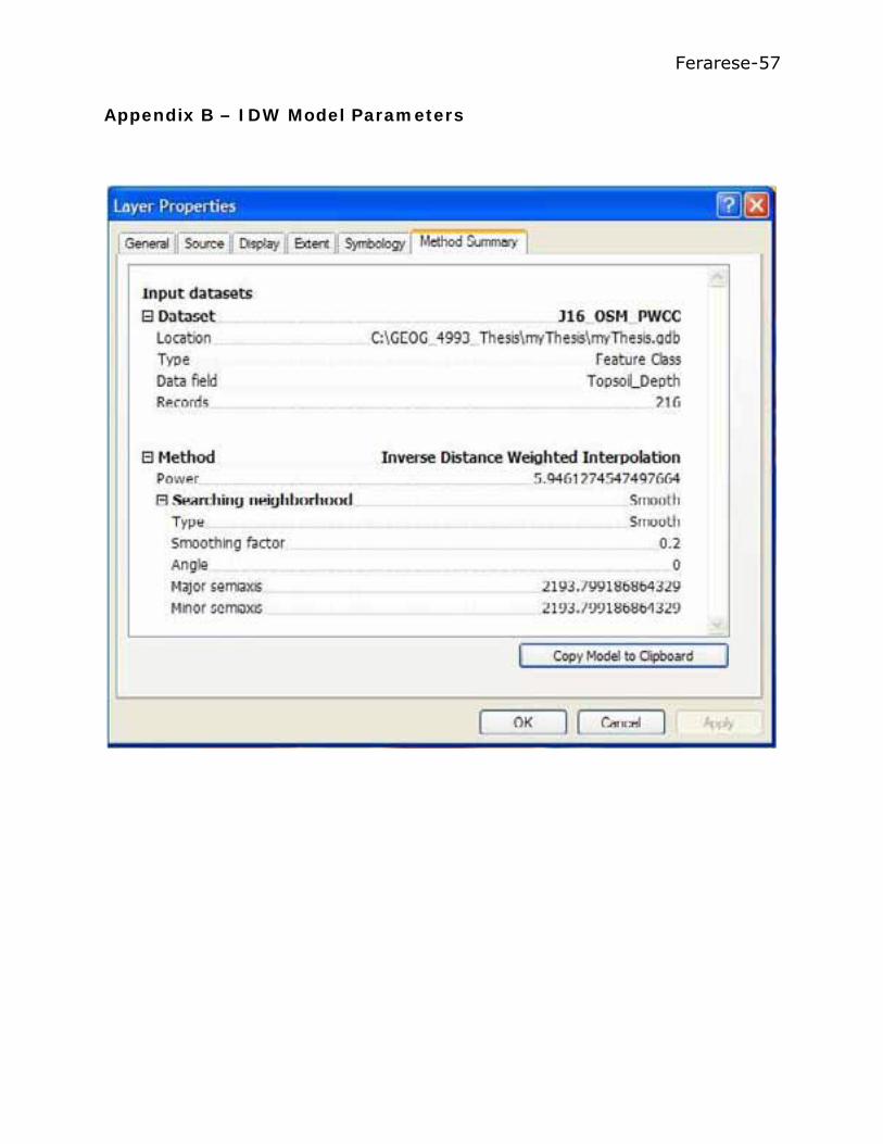
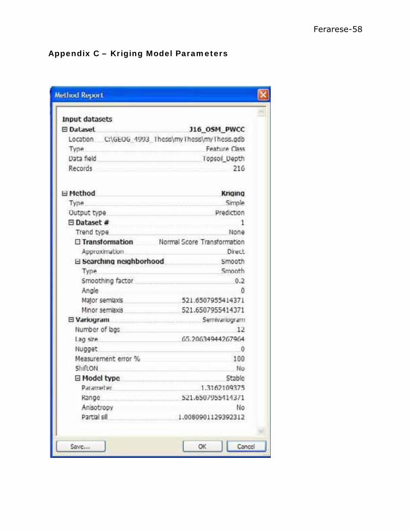
The method parameters for the IDW and the Simple Kriging models

that were used to create the predicted surfaces are listed in Appendix B and

C, respectively.

Cross-validation summary statistics and scatter plots are produced as

part of the output from the Geostatistical Analyst tools. The statistics and

plots were examined to determine how the interpolation models performed.

In addition to the summary statistics and plots, geostatistical methods

(Kriging) are equipped with the ability to produce a separate surface that

displays the standard error on the predicted surface. For the Simple Kriging

Ferarese-45

model, this diagnostic was also performed and the additional surface

created.

Assuming the data is normal, or can be transformed to normality, it is

possible to create a probability surface that displays the likelihood of

exceeding or failing to exceed a critical value. For the topsoil-depth, the

critical value required by the permit is 24 inches of topsoil evenly distributed

over the entire area. In order to further assess if this was accomplished, a

probability surface was created.

Compare Models

Similar to assessing the validity of a single model, summary statistics

and plots were used to compare the IDW and Kriging prediction surfaces.

Although the number of statistics produced by the Geostatistical Analyst

program for IDW is fewer than for Kriging it remained possible to make the

assessment.

Results

Inspection of the topsoil-depth point values resulted in the knowledge

that the data did not conform to the Normal distribution but was skewed to

the left. Formal exploratory data analysis resulted in observation of several

potential outliers being present but further investigation supported the

choice to not exclude them from input into the surface model interpolation

procedures.

Ferarese-46

Two optimized prediction surfaces were created using the deterministic

IDW method and the geostatistical Simple Kriging method. Each surface was

classified in the same manner. Five classes were chosen in order to provide

for more unambiguous interpretation. The class breaks were determined

manually to support the best visualization towards the task of determining

the distribution of topsoil-depth across an area. Figure 21 shows the two

surfaces side by side. Both surfaces represent over distribution of topsoil in

similar general areas (green to yellow classes.) The IDW surface, known for

its potential to produce “bulls eyes” around data locations, predicted two

areas where the topsoil was expressly under applied, at 6-inches (red class),

but which the Kriging surface smoothed out.

Figure 21. IDW and Simple Kriging Prediction Surfaces.

Ferarese-47

Visualization from each surface concurs that overall the topsoil-depth

24-inch minimum requirement evenly distributed across the area was not

achieved. The vast majority of the areas represented in both surfaces predict

that the topsoil was distributed to a depth of between 6 and 20 inches.

Geostatistical interpolation methods allow for creation of surfaces that

quantify the error involved in the prediction surface. Figure 22 is a surface

showing the standard error of prediction on the Simple Kriging method

derived surface.

Figure 22. Standard Error of Prediction Surface for the Kriging Derived Prediction Surface.

Ferarese-48

The lighter white-ish areas indicate where the predicted surface

performed with less error and the red areas are where the error in the

prediction of unknown values is greater. Overall, the Simple Kriging surface

performed well with few areas of red and those areas generally tend to be in

places where sampling frequency was more sparse.

In addition to producing error surfaces the geostatistical interpolation

methods are also capable of producing surfaces that display probabilities in

areas where critical values are exceeded or, as in the case of minimum

topsoil-depth, not exceeded. Such probability maps operate under the

assumption that the data is normally distributed. The simple kriging method

that was used in this analysis allows for transformation of the data. The

Normal Standard Transformation was utilized on this dataset to produce

more normal characteristics in the data prior to surface creation.

A surface describing the probability that the study area contains a

topsoil-depth distributed to the required minimum 24-inches is displayed in

Figure 23. The surface shows that only a few places (grey areas) are 68%

likely to contain the minimum topsoil-depth. The majority of the area has

less than 95% likelihood the requirement was met, and a large portion of

the area virtually did not meet the requirement (red areas).

Ferarese-49

Figure 23. Probability Surface of 24-inch Minimum Requirement.

The final determination involves quantifying which surface predicted

topsoil-depth distribution better, IDW or Kriging. Through utilization of the

statistics derived from cross-validation it is possible to compare the

performance between surfaces. Figure 24 is the comparison of the cross-

validation statistics and scatter plots between the IDW and Kriging surfaces

created in this analysis.

Ferarese-50

Figure 24. Cross-validation Statistics for IDW and Simple Kriging Comparison.

The scatter plots of measured verses predicted values in Figure 24

may at first suggest that the IDW method outperformed Kriging by virtue of

the tighter correlation observed on the IDW plot to the 1:1 line. The

predicted line is the thicker blue one. But the IDW slope is usually less than

the slope line in Kriging due to a property of the method that tends to under

estimate large values and over estimate smaller values. (Johnston, 2001)

Ferarese-51

The summary statistics are presented below the scatter plots in Figure

24. It is expected that in a good model, the prediction errors will be

unbiased and therefore near zero. The mean error in the IDW model is 0.24

and in the Kriging model it is 0.068. Also expected of a good model is that

the root-mean-square prediction error (RMSPE) be minimized because the

closer the predictions are to true values the smaller it will be. The RMSPE in

the IDW model is 4.17 and in the Kriging model it is 4.71.

Conclusion

Coal-mining operations, albeit the predominate means of

acquiring the fuel necessary for production of electricity in the U.S., also

come with severe adverse consequences to the land and environment.

Creation of cell-based analysis prediction surfaces from sampled

topsoil-depth point values can aid in determining how evenly a mine

operator has spread the required minimum depth of topsoil over newly

reclaimed areas on surface coal mines.

Use of prediction surfaces from sampled topsoil-depth point values

could help to more accurately evaluate topsoil replacement commitments

defined in surface coal mine permits and could help to ensure better

reclamation.

With a topsoil distribution surface layer in hand it will be more

apparent which areas require additional topsoil and from which areas excess

topsoil may be acquired. With a continuous surface map it can more readily

Ferarese-52

be determined what is necessary in order to comply with the requirement of

an evenly distributed topsoil depth.

The ability to make balanced environmental decisions necessitates

taking into consideration interacting factors. Geostatistical tools and

methods provide this capacity towards more appropriately and accurately

defined environmental analysis but it must be recognized that models are

only approximations of reality and must not be considered exact

representations.

Future Opportunities

In efforts to further quantify the interpolated surfaces created in this

report and apply their result to complementary coal mining scenarios it could

prove valuable to utilize remote sensing technology in concert with them.

With the use of high-resolution, multi-spectral satellite imagery collected

over several growing seasons at the areas of interest described in this report

it would be possible to classify the imagery using the infra-red band and

calculate vegetative indices. It would be possible to compare areas where

vegetation growth may not be occurring successfully with the predicted

probability maps displaying areas where topsoil-depth was predicted to be

less than the optimum 24 inches.

It would prove ideal for non-spatially trained personnel in the mining

industry to have access to automatic production of topsoil-depth prediction

surfaces without having to be intimately familiar with the intricate decision

Ferarese-53

making involved. This analysis showed there is little difference between

deterministic IDW and the many decisions required in geostatistical Kriging,

at least for this study site. Similar findings (Chaplot, et al., 1999)

determined there is little difference as long as the sampling density is high.

But what formulates high sampling density among newly reclaimed topsoil

distribution areas remains unknown. If it were determined that the IDW

method served to produce a reliable surface model of topsoil distribution

then it could be incorporated into an ESRI© ModelBuilderTM model or script

for use, perhaps even incorporated as a geoprocessing service in an online

web application.

Ferarese-54

References

Amirinejad, Ali. 2011. Assessment and mapping of spatial variation of soil physical health in a farm. Geoderma 160 (3/4) (-01-15): 292.

Burrough, Peter, A. and McDonnell, Rachael, A. “Principles of Geographic Information Systems”, Oxford University Press, 1998.

Chaplot, Vincent. 2006. Accuracy of interpolation techniques for the derivation of digital elevation models in relation to landform types and data density. Geomorphology (Amsterdam, Netherlands) 77 (1/2) (-07-15): 126.

Demirhan, M. 2003. Performance evaluation of spatial interpolation methods in the presence of noise. International Journal of Remote Sensing 24 (6) (-03-20): 1237.

De Smith, Michael, J., Goodchild, Michael, F., and Longley, Paul, A., “Geospatial Analysis – A Comprehensive Guide to Principles, Techniques and Software Tools – 3rd edition”, Winchelsea Press, 2011.

Evans, L. Keith. 2008. A Cause and Effect Relationship between Antiquated Mapping Standards/Techniques and Recent Mining Accidents and Fatalities. Paper presentation at the 2008 Geospatial Conference and 2nd National Meeting of SMCRA Geospatial Data Stewards, Atlanta, GA.

Fu, Pinde and Sun, Jiulin, “Web GIS Principles and Applications”, ESRI Press, 2011.

Greb, Stephen F., Eble, Cortland F., Peters, Douglas C., and Papp, Alexander R., “Coal and the Environment”, American Geological Institute, 2006.

Green, Kass. 2009. Together at Last. ArcUser Online, Fall 2009.

Hill, Michael, 2004. 3-D Modeling of Large Anthracite Open Pit Mining Operations to Assist in Pennsylvania’s Conversion to Conventional Bonding. Paper presentation at the 2004 Advanced Integration of Geospatial Technologies in Mining and Reclamation, 2004, Atlanta, GA.

Johnston, Kevin, Ver Hoef, Jay, M., Krivoruchko, Konstantin, and Lucas, Neil, “Using ArcGIS Geostatistical Analyst”, ESRI Press, 2001.

Ferarese-55

Krivoruchko, Konstantin, “Spatial Statistical Data Analysis for GIS Users”, ESRI Press, 2011.

Lamont, Samuel, J., Robert, Eli, N., Fletcher, Jerald, J., and Galya, Thomas, Cumulative Hydrologic Impact Assessments of Surface Coal Mining Using WCMS-HSPF, Paper presentation at the 2008 Geospatial Conference and 2nd National Meeting of SMCRA Geospatial Data Stewards, Atlanta, GA.

Liu, Dianwei, Spatial distribution of soil organic carbon and analysis of related factors in croplands of the black soil region, northeast china. Agriculture, Ecosystems & Environment 113 (1-4) (-04-01): 73, 2006.

Lloyd, Christopher, D., “Spatial Data Analysis”, Oxford University Press, 2010.

Mitchel, Andy, “The ESRI Guide to GIS Analysis – Volume 1: Geographic Patterns and Relationships”, ESRI Press, 1999.

--------, “The ESRI Guide to GIS Analysis – Volume 2: Spatial Measurements and Statistics”, ESRI Press, 2005.

Rohrer, Chris, S., Miles, Jenny, Smith, Daniel, and Fluke, Steve. 2008. GIS as a Prioritization and Planning Tool in Abandoned Mine Reclamation. Paper presentation at the 2008 Geospatial Conference and 2nd National Meeting of SMCRA Geospatial Data Stewards, Atlanta, GA.

U.S. Department of the Interior, Office of Surface Mining Reclamation and Enforcement, National Technical Training Program, “Basic Inspection Workbook”, 2007

Wingle, William, L. 1992. Examining Common Problems Associated with Various Contouring Methods, Particularly Inverse-Distance Methods, Using Shaded Relief Surfaces. Geotech ‘92 Conference Proceedings, Lakewood, Colorado, 1992.

Zhang, Xuesong. 2009. GIS-based spatial precipitation estimation: A comparison of geostatistical approaches. Journal of the American Water Resources Association 45 (4) (-08-01): 894.

Ferarese-56

Appendix A – List of Acronyms

CHIA Cumulative Hydrologic Impact Assessment

DEM Digital Elevation Model

DOI Department of Interior

EPA Environmental Protection Agency

ESRI Environmental Systems Research Institute

GIS Geographic Information System

GPS Global Positioning System

HSPF Hydrologic Simulation Program-Fortran

IDW Inverse Distance Weighted

LOM Life of Mine

OSM Office of Surface Mining and Enforcement

PA-DEP Pennsylvania Department of Environmental Protection

QQ Quantile-Quantile Plot

RMSE Root-mean-square Error

RMSPE Root-mean-square Predicted Error

SMCRA Surface Mining Control and Reclamation Act

SOC Soil Organic Carbon

WCMS Watershed Characterization and Modeling System

WVU West Virginia University

Ferarese-57

Appendix B – IDW Model Parameters

Ferarese-58

Appendix C – Kriging Model Parameters