Supporting Information

Monitoring CO2 invasion processes at pore scale using Geological Labs on Chip

S. Morais, N. Liu, A. Diouf, D. Bernard, C. Lecoutre, Y. Garrabos, S. Marre*

Electronic Supplementary Material (ESI) for Lab on a Chip.This journal is © The Royal Society of Chemistry 2016

S1 – Microfabrication procedure and set-up

Microfabrication

Fig. S1 summarized the microfabrication procedure used for developing the GLoCs devices.

Fig. S1.1 Scheme of the GLoCs microfabrication procedure.

In details: The network is etched on a silicon wafer (<100> orientation perpendicular to the

surface) purchased from BT Electronics, Inc. The purchased silicon wafer is already coated with

a thermal silicon oxide layer of 500 nm on both sides. The photolithography process consists

in:

(i) Spin coating a thin layer (4 µm) of positive photoresist (S1818 from Shipley),

(ii) Exposing the coated wafer with UV light (6 mW/cm2, 45 sec) through a soft mask.

The positive photoresist exposed to UV through the mask is removed from the

silicon oxide surface with a developer (MF319 from Shipley).

(iii) Removing the silicon dioxide with a buffered HF solution (hydrofluoric acid + NH4F)

in water (Sigma Aldrich).

(iv) Dissolving the remaining photoresist with acetone.

The wet etching of the silicon is done with a solution of Tetramethylammonium hydroxide

(TMAH) 25% in water (Sigma Aldrich) at an etching rate of 0.7 µm/min. A thin silicon oxide

layer is deposited onto the etched silicon wafer using a wet oxidation process conducted in an

oven at 1000°C during 2 hours under water saturated atmosphere. The injection holes are

drilled with a sandblasting equipment. Eventually, the etched silicon wafer is anodically bonded

to a Pyrex wafer.

Set-up

The micro fabricated pore network was then connected to the external inlet/outlet tubing

thanks to a homemade compression fitting:

Fig. S1.2 Scheme of the compression fitting used in this study. The scheme was adapted from:

“Marre, S., Adamo, A., Basak, S., Aymonier, C. & Jensen, K. F. Design and Packaging of Microreactors

for High Pressure and High Temperature Applications. Ind. Eng. Chem. Res. 49, 11310–11320 (2010).”

A general picture of the micromodel / compression fitting assembly is given hereafter:

Fig. S1.3 Picture of the [micromodel + Compression fitting] assembly.

S2 - Wetting contact angle measurements

The contact angle measurement are obtained by an image analyses with ImageJ1 and the contact angle plug-in of Marco Brugnara.2 Two types of images were used for these measurements. First, the interface of water and CO2 into a straight feeding microchannel (Fig S2-a.). Here, the contact angle corresponds to the angle between the wall of the channel and the tangent to the interface meniscus (Fig S2-b.). Secondly, the shape of the dome on the silica plots are also used for these measurements. The contact lines between the water and the solid are curved (Fig S2-c.), the contact angle is here between the tangent of the circular plot and the tangent the water dome (Fig S2-d.). The obtained values for are reported in Table S2.

Fig. S2 Example of observations and further measurements of the contact angle at p = 4.5 MPa T = 28 °C with Micromodel M2. (a, b) inside the feeding microchannel and (c, d) around a circular plot.

Table S2 Contact angle values measured depending on the operating conditions.

p (MPa) T (°C) Phase (deg)

4.5 28 Gas 25.7 ± 3.1

6 28 Gas 30.7 ± 1.9

8 28 Liquid 39.2 ± 2.4

8 50 Supercritical 36.7 ± 2.6

8 75 Supercritical 35.7 ± 2.1

1 Abramoff, M. D.; Magalhaes, P. J.; Ram, S. J. Image Processing with ImageJ. Biophotonics Int. 2004,

11 (7), 36−42. (52) 2 M. Brugnara, contact Email: marco.brugnara@ing. unitn.it)

(a) (b)

(c) (d)

100 µm 100 µm

100 µm 100 µm

S3 – General properties of the fluids depending on the p and T conditions

Table S3 summarizes the thermophysical properties of water and CO2 in the studied conditions. Density

and viscosity were obtained from the NIST,3 while the interfacial tension values were obtained from

the literature (references mentioned in the Table).

Table S3 Thermophysical properties of water and CO2 in the studied conditions.

P (MPa)

T (°C)

Phase

H2O viscosity

µH2O (µPa·s)

H2O density ρH2O

(kg m-3)

CO2 viscosity

µCO2 (µPa·s)

CO2 density ρCO2

(kg m-3)

Viscosity ratio log M (M= µCO2/

µH2O)

Interfacial tension γ (mN·m-1)

4.5 28 Gas 831.9 998.2 16.3 107.7 -1.17 43.24

6 28 Gas 831.7 998.9 18.1 178.0 -1.66 36.04

8 28 Liquid 831.5 999.7 60.7 736.5 -1.14 30.34

8 50 Supercritical 548.3 991.5 20.5 219.2 -1.43 37.55

8 75 Supercritical 379.8 978.3 20.0 166.5 -1.28 38.66

3 http://webbook.nist.gov/chemistry/fluid/ 4 Georgiadis, A., Maitland, G., Trusler, J. P. M. & Bismarck, A. Interfacial Tension Measurements of the (H2O +

CO2) System at Elevated Pressures and Temperatures †. J. Chem. Eng. Data 55, 4168–4175 (2010). 5 Chun, B.-S. & Wilkinson, G. T. Interfacial tension in high-pressure carbon dioxide mixtures. Ind. Eng. Chem.

Res. 34, 4371–4377 (1995). 6 Bachu, S., Bennion, D. B., Clark, K., Nw, R. & Tn, A. Interfacial Tension between CO 2 , Freshwater , and Brine

in the Range of Pressure from ( 2 to 27 ) MPa , Temperature from ( 20 to 125 ) ° C , and Water Salinity from ( 0 to 334 000 ) mg · L - 1. 765–775 (2009).

S4 – Dimensionless numbers for the considered experimental conditions

Table S4 summarizes the calculated dimensionless numbers (Log Ca, Log M and Re) for the different experiments performed in the frame of this study. Ca was calculated using Eq. 2.

Table S4 Dimensionless numbers (Log Ca, Log M and Re for the considered experimental conditions.

Micromodel M1 M2

p.T

conditions

Qpump

(µl min-1) Log Ca Log M

uCO2

(m s-1) Re Log Ca Log M

uCO2

(m s-1) Re

4.5 MPa 28 °C

100 -3.93 -1,71 0.28 41.1 -3.85 -1,66 0.33 38.5

6 MPa 28°C

100 -4.02 -1,66 0.17 37.9 -3.94 -1,71 0.21 35.5

8 MPa

28°C 100 -3.99 -1,14 0.04 11.5 -3.92 -1,14 0.05 10.8

8 MPa

50°C 100 -4.02 -1,43 0.14 34.1 -3.94 -1,43 0.17 31.9

8 MPa 75°C

100 -3.92 -1,28 0.19 35.0 -3.84 -1,28 0.22 32.7

8 MPa 50°C

200 -3.72 -1,43 0.29 68.2 -3.64 -1,43 0.34 63.9

S5 – Location of our experiments in the Lenormand’s stability diagram7

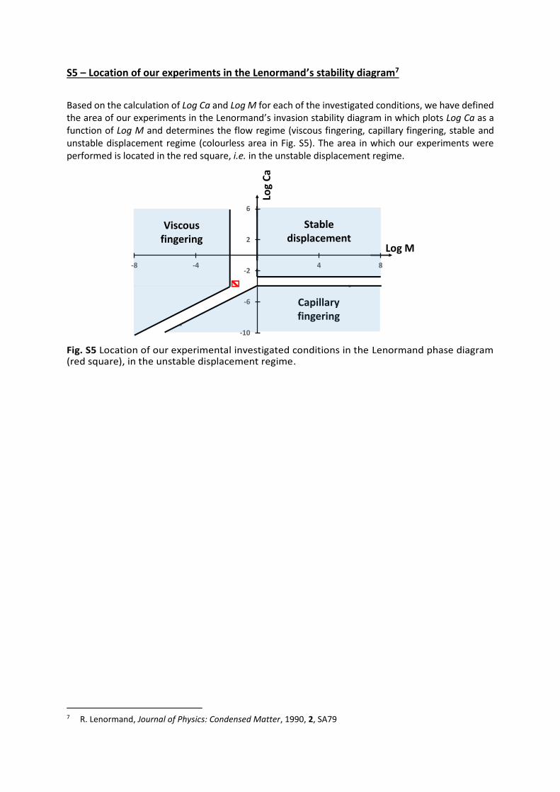
Based on the calculation of Log Ca and Log M for each of the investigated conditions, we have defined the area of our experiments in the Lenormand’s invasion stability diagram in which plots Log Ca as a function of Log M and determines the flow regime (viscous fingering, capillary fingering, stable and unstable displacement regime (colourless area in Fig. S5). The area in which our experiments were performed is located in the red square, i.e. in the unstable displacement regime.

Fig. S5 Location of our experimental investigated conditions in the Lenormand phase diagram (red square), in the unstable displacement regime.

7 R. Lenormand, Journal of Physics: Condensed Matter, 1990, 2, SA79

-10

-6

-2

2

6

-8 -4 0 4 8

Titre du graphiqueLog

Ca

Log M

Capillaryfingering

Stable displacement

Viscousfingering

S6 – Drying mechanism as a function of the temperature

Figure S6 shows the influence of temperature over the drying kinetics, demonstrating a faster drying process at higher temperature (75°C compared to 50°C both at 8 MPa). Typical pictures of the porous medium are shown as a function of the injection time from t = 5s to t = 75s).

Fig. S6 Drying process for different times during the invasion experiment (with micromodel

M1) at two different temperatures (50 and 75°C).

t = 5 s t = 35 s t = 50 s t = 75 s

8 MPa

50 C

8 MPa

75 C

Fig S3 Drying process for different times during the invasion experiment (Micromodel M1)

S7 – Solubility of CO2 in water as a function of temperature and pressure

Fig. S7 Solubility data of water in CO2 at different pressures and temperatures (adapted from

Spycher, N., Pruess, K. & Ennis-King, J. CO2-H2O mixtures in the geological sequestration of

CO2. I. Assessment and calculation of mutual solubilities from 12 to 100°C and up to 600 bar.

Geochim. Cosmochim. Acta 67, 3015–3031 (2003)).