Supporting Information

Spin-Chemical Effects on Intramolecular

Photoinduced Charge Transfer Reactions in

Bisphenanthroline Copper(I)-Viologen Dyad

Assemblies

Megan S. Lazorski,*a† Igor Schapiro,b† Ross S. Gaddie,a Ammon P. Lehnig,a Mihail Atanasov,b

Frank Neese,*b Ulrich E. Steiner,*c and C. Michael Elliotta‡

aDepartment of Chemistry, Colorado State University, Fort Collins, CO 80523. bMax Planck

Institute for Chemical Energy Conversion, D-45470 Mülheim an der Ruhr, Germany.

cDepartment of Chemistry, University of Konstanz, Universitätsstraße 14, Konstanz, 78457,

Germany

Contents

A. LIGAND AND COPPER COMPLEX SYNTHESIS 2

B. OPTICAL SETUP FOR TRANSIENT ABSORPTION SPECTROSCOPY 6

SIGNAL PROCESSING 7

C. SOLVENT EFFECTS ON INITIAL AMPLITUDE OF MEC+A48+ 8

D. QUANTUM CHEMISTRY 9

S1

Electronic Supplementary Material (ESI) for Chemical Science.This journal is © The Royal Society of Chemistry 2020

GEOMETRY OPTIMIZATION 9RESULTS OF THE GEOMETRY OPTIMIZATION 10CALCULATION OF EPR PARAMETERS 19G-TENSOR 20HYPERFINE COUPLING CONSTANTS 22

E. THEORETICAL CALCULATION OF CT DECAY TIME 25

F. REFINED ANALYSIS OF MCMILLIN SCHEME 28

G. EMISSION DECAY CURVES 33

H. SPIN MOTION AND SPIN RELAXATION 34

SPIN RELAXATION 34ON THE ROLE OF ANISOTROPIC HYPERFINE COUPLING AT LOW MAGNETIC FIELDS 35MOMENT OF INERTIA 37ESTIMATION OF CLASSICAL RATE CONSTANTS REPRESENTING COHERENT MIXING PROCESSES 38

S/T0 mixing by g-mechanism 38General S/T0 mixing and S/T and T0/T mixing in zero field by isotropic hfc 39

ADVANCED SEMICLASSICAL THEORY 41SUPPLEMENTARY DIAGRAMS 44

A. Ligand and Copper Complex Synthesis

Other than the following exceptions, all starting materials and solvents were solvent grade or better,

obtained from commercial sources, and used without further purification. The 1,2-difluorobenzene (dfb)

was obtained from Oakwood Products, Inc. and run through a column of neutral, activated Al2O3 before

use. The hydrazine sulfate used in the synthesis of Me-Diol (see Scheme S1) was recrystallized from water

and dried thoroughly in the vacuum oven before use. Tetrakis(acetonitrile)copper(I) tetrafluoroborate

([Cu(ACN)4]+BF4-) was recrystallized from acetonitrile before use and stored in a dessicator. UltimAr

acetonitrile (ACN) was obtained from MACRON Chemicals. DriSolv dimethylformamide (DMF), OmniSolv

dichloromethane (DCM), and OmniSolv methanol (MeOH) were obtained from EMD Chemicals. Potassium

tetrakis(pentafluorophenyl)borate was obtained from Boulder Scientific. Tris(bipyridine)ruthenium(II)

hexafluorophosphate ([Ru(bpy)3]2+(PF6-)2) was synthesized as published previously.1 Solutions of MeOH in

dfb are reported as v/v percentage. Literature methods were used to prepare the 2,9-di(R=methyl or

phenyl)-1,10-phenanthroline-5,6-diol (R-Diol) from Scheme S1, as well as its precursor the 2,9-

di(R=methyl or phenyl)-1,10-phenanthroline-5,6-dione (R-Dione).2–6 In addition to structural verification

by 1H NMR, the purity of intermediates and final ligands was also typically verified by silica gel TLC. In the

S2

case of compounds which are charged, the elution solvent was 5:4:1 acetonitrile:water:KNO3 (sat. aq).

Static UV-Visible spectra were obtained using air-tight cells (vide infra) and an Agilent 8453 diode array

spectrometer.

Sche

N NRR

OHHO

XXN N +

Ctoluene

N N

X

+ 2.2N N

RR

OO

N

N

N

N

+X-

+ +PF6-

N NRR

OO

N

N

N

N+ +ClO4-

+ +

+ 3 CH3I CH3CNDMF, under Ar

XBM

PF6-

1. 45 C2. NaClO4

1. mol K2CO32. Sonicate3. NH4PF6

ClO4-

ClO4- ClO4

-

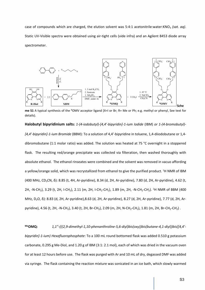
R-Diol R4OMQ R4OMVROMQ ROMV

me S1 A typical synthesis of the ROMV acceptor ligand (X=I or Br; R= Me or Ph; e.g. methyl or phenyl, See text for details).

Halobutyl bipyridinium salts: 1-(4-iodobutyl)-[4,4’-bipyridin]-1-ium Iodide (IBM) or 1-(4-bromobutyl)-

[4,4’-bipyridin]-1-ium Bromide (BBM): To a solution of 4,4’-bipyridine in toluene, 1,4-diiodobutane or 1,4-

dibromobutane (1:1 molar ratio) was added. The solution was heated at 75 °C overnight in a stoppered

flask. The resulting red/orange precipitate was collected via filteration, then washed thoroughly with

absolute ethanol. The ethanol rinseates were combined and the solvent was removed in vacuo affording

a yellow/orange solid, which was recrystallized from ethanol to give the purified product. 1H NMR of IBM

(400 MHz, CD3CN, δ): 8.85 (t, 4H, Ar-pyridine), 8.34 (d, 2H, Ar-pyridine), 7.80 (d, 2H, Ar-pyridine), 4.62 (t,

2H, -N-CH2), 3.29 (t, 2H, I-CH2), 2.11 (m, 2H, I-CH2-CH2), 1.89 (m, 2H, -N-CH2-CH2). 1H NMR of BBM (400

MHz, D2O, δ): 8.83 (d, 2H, Ar-pyridine),8.63 (d, 2H, Ar-pyridine), 8.27 (d, 2H, Ar-pyridine), 7.77 (d, 2H, Ar-

pyridine), 4.56 (t, 2H, -N-CH2), 3.40 (t, 2H, Br-CH2), 2.09 (m, 2H, N-CH2-CH2), 1.81 (m, 2H, Br-CH2-CH2) .

MeOMQ: 1,1”-(((2,9-dimethyl-1,10-phenanthroline-5,6-diyl)bis(oxy))bis(butane-4,1-diyl))bis([4,4’-

bipyridin]-1-ium) Hexafluorophosphate: To a 100 mL round bottomed flask was added 0.510 g potassium

carbonate, 0.295 g Me-Diol, and 1.20 g of IBM (3:1: 2.1 mol), each of which was dried in the vacuum oven

for at least 12 hours before use. The flask was purged with Ar and 10 mL of dry, degassed DMF was added

via syringe. The flask containing the reaction mixture was sonicated in an ice bath, which slowly warmed

S3

to 45 °C due to the sonication, and sonicated at 45 °C for 12 hours. The DMF was removed in vacuo and

the resulting viscous brown oil was sonicated in excess water. The water rinseates were filtered through

Celite to remove a black, tarry byproduct. The aqueous filtrate was collected, reduced in volume,

precipitated by adding solid NH4PF6, and the resulting precipitate was collected via centrifugation. The

crude product was purified by dissolving in hot MeOH, and filtering through celite. As the filtrate cooled,

the product precipitated from solution as a light beige solid which was collected by filtration. 1H NMR (400

MHz, CD3CN, δ): 8.86 (dd, 4H, Ar-pyridine), 8.74 (d, 4H, Ar-pyridine), 8.41 (d, 2H, 4,7-phen), 8.27 (d, 4H,

Ar-pyridine), 7.77 (dd, 4H, Ar-pyridine), 7.54 (d, 2H, 3,8-phen), 4.62 (t, 4H, N-CH2), 4.25 (t, 4H, O-CH2), 2.76

(s, 6H, CH3), 2.25 (m, 4H, -O-CH2-CH2), 1.89 (m, 4H, -N-CH2-CH2). HRMS: ESI/APCI-TOF m/z (relative

intensity): [(M-PF6)+H]+ calcd for C42H42F6N6O2P, 807.3006; found 807.3009.

MeOMV: 1’,1”’-(((2,9-dimethyl-1,10-phenanthroline-5,6-diyl)bis(oxy))bis(butane-4,1-diyl))bis(1-methyl-

[4,4’bipyridine]-1,1’-diium) Perchlorate: To a cold solution of 0.10 g of MeOMQ in 2 mL of ACN was added

20 μL of methyl iodide (1:3 mol). A Teflon lined vial cap was placed on the reaction vial which was heated

to 45 °C for 24 hrs. The resulting red was filtered, rinsed with acetonitrile, and subsequently rinsed with

MeOH. The MeOH rinsate was collected and 1 mL of NaClO4 (sat’d) in MeOH was added. The beige

precipitate was collected via filtration and rinsed with 15 mL hot MeOH. To the hot MeOH rinsate was

added 5 mL of isopropanol and the solution was quickly cooled to -17 °C. The product was collected as

light beige solids. 1H NMR (400 MHz, CD3CN, δ): 8.96 (d, 4H, Ar-pyridine), 8.86 (d, 4H, Ar-pyridine), 8.48

(d, 2H, 4,7-phen), 8.40 (d, 8H, Ar-pyridine), 7.60 (d, 2H, 3,8-phen), 4.74 (t, 4H, N-CH2), 4.41 (s, 6H, CH3-

pyridine), 4.28 (t, 4H, O-CH2), 2.80 (s, 6H, 2,9-phen-CH3), 2.32 (m, 4H, -O-CH2-CH2), 1.97 (m, 4H, -N-CH2-

CH2). HRMS: ESI/APCI m/z (relative intensity): [M-ClO4-]+ calcd for C44H48Cl3N6O14, 991.2271; found

991.2267.

PhOMQ: 1,1”-(((2,9-diphenyl-1,10-phenanthroline-5,6-diyl)bis(oxy))bis(butane-4,1-diyl))bis([4,4’-

bipyridin]-1-ium) Perchlorate: In a typical reaction, in an inert atmosphere box 50 mg of P-Dione was

added to a 20 mL scintillation vial along with 6.4 mg of sodium metal (2 eq.) and 5 mL of anhydrous DMF,

S4

which was stirred overnight resulting in a dark red solution. Ammonium nitrate (19.9 mg, 1.8 eq.), which

had been previously dried at 80 C in a vacuum oven, was added to the solution. The resulting diol solution

was amber in color and used without isolation. Anhydrous cesium carbonate (135.0 mg, 3.0 eq.) and solid

BBM (128.4 mg. 2.5 eq.) were added to the diol solution and the reaction was stirred for 24 hours under

inert atmosphere. On the benchtop, a few drops of H2O and a small piece of dry ice were added to the

reaction to neutralize any excess Cs2CO3. After all of the solid CO2 had sublimed, the solvent was removed

under vacuum to yield a dark brown tar.

The residue above was extracted thoroughly with MeOH, the MeOH extracts were combined, and a

concentrated methanolic solution of NaClO4 was added dropwise while swirling to afford a grey/tan

flocculent precipitate. The solution was centrifuged to isolate the solid. The isolated solids were re-

suspended in pure MeOH and re-centrifuged. The product was dried in vacuo, dissolved in ACN (ca. 10

mL) and transferred to a scintillation vial. Approximately 50 mg of activated silica gel (Aldrich 70-230

mesh) was added to this solution and the vial tightly capped. The vial was then placed on its side on a

rocker table and roll back and forth overnight. The light-yellow solution was decanted from the silica gel

into a round bottom flask and the silica washed with several ca. 1 mL portions of ACN, which were

combined with product solution in the round bottom flask. Approximately 50 mg of NaClO4(s) was added

to the flask and the ACN removed in vacuo to yield a light yellow/tan residue. Approximately 10 mL of

H2O was added to the flask and product was collected by vacuum filtration and washed with several

portions of H2O. 1H NMR (400 MHz, CD3CN, δ): 8.81 (d, 4H, Ar-pyridine), 8.73 (d, 4H, Ar-pyridine), 8.63 (d,

2H, 4,7-phen), 8.44 (d, 4H, 2,9-phen-o-Ph), 8.25 (d, 2H, 3,8-phen), 8.23 (d, 4H, Ar-pyridine), 7.73 (d, 4H,

Ar-pyridine), 7.64 (t, 4H, 2,9-phen-m-Ph), 7.56 (t, 2H, 2,9-phen-p-Ph), 4.62 (t, 4H, N-CH2), 4.35 (t, 4H, O-

CH2), 2.27 (m, 4H, O-CH2-CH2), 1.94 (m, 4H, N-CH2-CH2)

PhOMV: 1’,1”’-(((2,9-diphenyl-1,10-phenanthroline-5,6-diyl)bis(oxy))bis(butane-4,1-diyl))bis(1-methyl-

[4,4’bipyridine]-1,1’-diium) Perchlorate: The same procedure was followed as for converting the MeOMQ

to MeOMV with the following exceptions: after alkylation, conversion to the perchlorate salt was

accomplished by dissolving the mixed I-/ClO4- product PhOMV in a mixture of H2O/MeOH/acetonitrile and

S5

adding excess NaClO4(s) followed by removal of solvent by rotary evaporation. Water was then added to

the flask to suspend the product, which was isolated by vacuum filtration. 1H NMR (400 MHz, CD3CN, δ):

8.83 (d, 4H, Ar-pyridine), 8.76 (d, 4H, Ar-pyridine), 8.64 (d, 2H, 4,7-phen), 8.42 (d, 4H, Ar-pyridine), 8.32

(d, 4H, 2,9-phen--phenyl), 8.27(d, 2H, 3,8-phen-phenyl), 8.23 (d, 4H, Ar-pyridine), 7.67 (t, 4H, 2,9-phen-

phenyl), 7.60 (t, 2H, 2,9-phen-phenyl), 4.69 (t, 4H, N-CH2), 4.38 (t, 4H, O-CH2), 4.35 (s, 6H, N-CH3), 2.29 (m,

4H, O-CH2-CH2), 1.94 (m, 4H, N-CH2-CH2).

[Cu(I)(Rphen(OMV)24+)2]9+ (TPFB-)9: Di-(1’,1”’-(((2,9-dimethyl-1,10-phenanthroline-5,6-diyl)bis(oxy))bis

(butane-4,1-diyl))bis(1-methyl-[4,4’bipyridine]-1,1’-diium))copper(I) Tetrakis(pentafluorophenyl)

borate(MeC+A48+) or Di-(1’,1”’-(((2,9-diphenyl-1,10-phenanthroline-5,6-diyl)bis(oxy))bis(butane-4,1-

diyl))bis(1-methyl-[4,4’bipyridine]-1,1’-diium))copper(I) Tetrakis(pentafluorophenyl) borate (PhC+A48+): A

typical preparation of a stock solution of the diad complexes for spectral measurement (TA or UV-vis) is

as follows: To a vial containing 1 mL of ACN (UltimAr) was added 0.0052 g (1.5 molar xs) potassium

tetrakis(pentafluorophenyl)borate (TPFB-), 109 μL of a 9.2 mM ROMV solution in ACN, and 157 μl of a 3.2

mM solution of [Cu(ACN)4]+BF4- in ACN (2:1 molar ratio), in that order, after which the solvent was

removed in vacuo. The complex was then brought into the inert atmosphere box and dissolved in 2.5 mL

degassed dfb. 1H NMR of [Cu(I)(Mephen(OMV)24+)2]9+ (TPFB-)9 (400 MHz, CD3OD, δ): 9.28 (d, 4H, Ar-

pyridine), 9.15 (d, 4H, Ar-pyridine), 8.69 (d, 2H, 4,7-phen), 8.65 (d, 4H, Ar-pyridine), 8.60 (d, 4H, Ar-

pyridine), 7.73 (d, 2H, 3,8-phen), 4.88 (t, 4H, N-CH2), 4.50 (s, 6H, CH3-pyridine), 4.38 (t, 4H, O-CH2), 2.45

(m, 4H, -O-CH2-CH2), 2.31 (s, 6H, 2,9-phen-CH3), 2.11 (m, 4H, -N-CH2-CH2).

Since Cu(I) complexes suffer from inherent lability, the complexes must self-assemble in solution

through the method described above, precluding many standard methods of isolation, purification, and

characterization. To address this, detailed titration experiments were performed via 1H NMR, UV-vis and

cyclic voltammetry (CV) to verify the purity and stoichiometric ratio of the complexes as assembled. A

typical experiment would proceed as follows: two molar equivalents of the ROMV ligand was placed in an

appropriate solvent (For 1H NMR: typically CD3CN/CD2Cl2 (1:1 v/v) or CD3OD/CD2Cl2 (1:1 v/v); for UV-vis

and CV typically CH3CN, CH3OH, or a mixture of CH3CN or CH3OH with CH2Cl2 or 1,2-difluorobenzene) and

S6

a spectrum was recorded. After measuring the spectrum of the free ligand, a solution of [Cu(CH3CN)4](X-)

(X- = tetrafluoroborate (BF4-), perchlorate (ClO4

-), hexafluorophosphate (PF6-), tetrakis[3,5-

bis(trifluoromethyl)phenyl]borate (BARF-), or tetrakis(pentafluorophenyl)borate (TPFB-)) was

incrementally added to the solution, in either 0.25 or 0.5 molar equivalent aliquots, and a spectrum was

recorded after each addition. In all of these experiments, consistent, reproducible spectra were afforded.

In the 1H NMR experiments, differentiation of the mono- and di-substituted C-A dyads,

[Cu(ROMV)(solvent)2](X-) and [Cu(ROMV)2](X-), was facile and reproducible enough to enable relative

quantitation of each compound in solution within a few weight %, adding credence to the 1H NMR

assignments above. In the CV experiments, the obtained redox behavior of the ROMV was unaffected by

coordination, as expected based on the distance of the acceptor moiety from the coordination sphere.

However, coordination was verified by a copper stripping peak that emerges after the molar ratio exceeds

2:1 (R4OMV:Cu+), as is evident in Figure S1 for the C-A dyad with MeOMV. If the monosubstituted solvento

complex had formed, [Cu(ROMV)(solv)2]+(X-), the stripping peak would not have been observed until the

R4OMV:Cu+ ratio exceeded 1:1 stoichiometry. Additionally, the CV data was an excellent secondary

confirmation of the sample purity due to the lack of any other redox signals on the A scale over a wide

potential range.

Figure S1. A representative CV titration experiment verifying the formation of pure 2:1 homoleptic complexes with the 4OMV acceptor ligands. In this particular experiment, the electrolyte solution was 0.1 M tetrabutylammonium hexafluorophosphate (TBA+(PF6

-)) in optima acetonitrile (Working electrode: glassy

S7

carbon, Auxiliary electrode: Pt coil, Scan rate : 50 mV/sec, Initial potential sweep: negative). Inset: A shift in the peak potential is evident after the R4OMV:Cu+ ratio exceeds 2:1 stoichiometry as the stripping peak emerges.

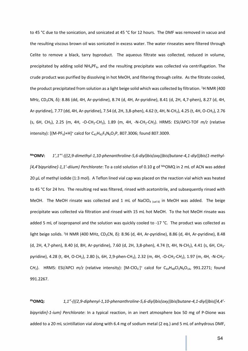
B. Optical Setup for Transient Absorption Spectroscopy

A. B.

PMT

Laser

Lamp

Sample ChopperWheel

Photodiode

OscilloscopeMono-

chromator

Signal= If/Ii

PMT

Laser

Lamp

Sample

ChopperWheel

Photodiode

OscilloscopeMono-

chromator

Signal= If/Ii

Electromagnet

Figure S2 Schematic of the transient absorption laser set-up. A) Set-up used to determine CT/CS lifetime and transient absorption spectra in absence of magnetic field. B) Set-up used to for determining lifetime of CT/CS and initial intensities in a magnetic field.

Signal Processing

The signal was processed as follows when the decay times of transient signals would be affected by the

time profile of the laser pulse. To correct for the finite duration of the pumping period, the observed

signals were fit using either Origin 7.5 advanced fitting function or a nonlinear regression fitting function

in the statistical computing software R7 which fit a differential equation simulating the excitation and

subsequent decay of CT state during and after each laser pulse.

Examples of the laser pulse profile measured by a Thorlabs DET210 high speed photodiode detector

(rise/fall time 1 ns) are shown in Figure S3. They can be reproduced rather well by Gaussian profiles with

FWHM of 4.0 ± 0.1 ns.

S8

Lamp

Laser

Monochromator PMT

Lamp

Laser

Monochromator PMT

Figure S3 Laser time profiles measured with the photodiode and Gaussian fits.

Figure S4 Detected signals at various fields (blue). Laser profile, represented by a Gaussian of 4.0 ns FWHM (orange), result of ODE-fit (red), residualx10 (dashed, black). The resulting decay times/rate constants of decay are given as insets.

The transient signals were measured with a Hamamatsu PMT R2496 (fast time response 0.6 ns). Examples

of recorded signals and ODE fits are shown in Figure S4. In the fits, Gaussian time profiles of the laser

pulse were used with adjustable width. The best fits were obtained with a FWHM value of 4.0 ns, which

nicely fits the laser profile widths measured with the photodiode.

C. Solvent Effects on Initial Amplitude of MeC+A48+

As the MeOH concentration increases, so does the initial amplitude of the TA signal for MeC+A48+

(Figure S5A). However, there is a concomitant increase in the magnitude of the [Cu(I)P2] MLCT

band in the static absorption spectrum with the first several additions of MeOH to the cell(Figure

S5B). This may be due to a change in the absorption coefficient, but, although no solids were

visible in the initial solution, the increased absorbance, in this case, may at least partially be due

S9

to the increased solubility of the complex when MeOH is present. This explanation is supported

by the fact that there is also essentially no difference in the MLCT band shape in the presence and

absence of MeOH in solution. Furthermore, a slight decrease in the initial amplitude of the CT

absorbance for the highest MeOH concentration is consistent with the simple dilution of the

MeC+A48+ concentration with the added volume of MeOH (evident in both the static and TA

spectra). The static absorbance at λmax for 0% and 2% MeOH concentrations differ by ca. 30%

whereas the maximum ΔA in the transient absorbance differs by approximately a factor of two.

This difference is a result of the short lifetime for the CT state in the absence of MeOH (see

discussion of the fitting approaches in the Experimental Section). When the MaxΔA values

obtained from the ODE fits are compared for the 0 and 2% MeOH solutions, their values match

the difference in the ground state absorbance (i.e., ca. 30%; cf. table inserts in Figure S5B). This

can be seen more clearly from the values of MaxΔA normalized for the absorbance at λmax

presented in the last column of the table insert in Figure S5B. From these data, there is an

apparent increase in the initial amount of CT formed per unit MeC+A48+. There are several possible

S10

Figure S5 (A) The effect on the single-wavelength TA of MeC+A48+ in dfb/X% MeOH at 396 nm (λex=475 nm), and (B)

static spectra as a function of %[MeOH]. The table inset in (A) provides the measured delta absorbance at t=0 (ΔAt0), the calculated delta absorbance at t=0 using the ODE-fitting technique (MaxΔA), and the lifetime resulting from the ODE fit (τ1). The table inset in (B) provides the total change in MaxΔA for comparison to the change in static absorbance with MeOH concentration. The data shown in (A) were obtained with a small (25 mT) applied magnetic field due to a logistical issue; however, the effect of a magnetic field on the CT lifetime is small at this field and are thus still accurate for zero field within a few percent.

causes for this change in initial amplitude. In sum, this effect is likely due to a combination of

factors: increased solubility, longer CT, and an approximately 10% increase in initial CT state

formation as MeOH concentration increases from 0-5%.

D. Quantum Chemistry

Geometry optimization

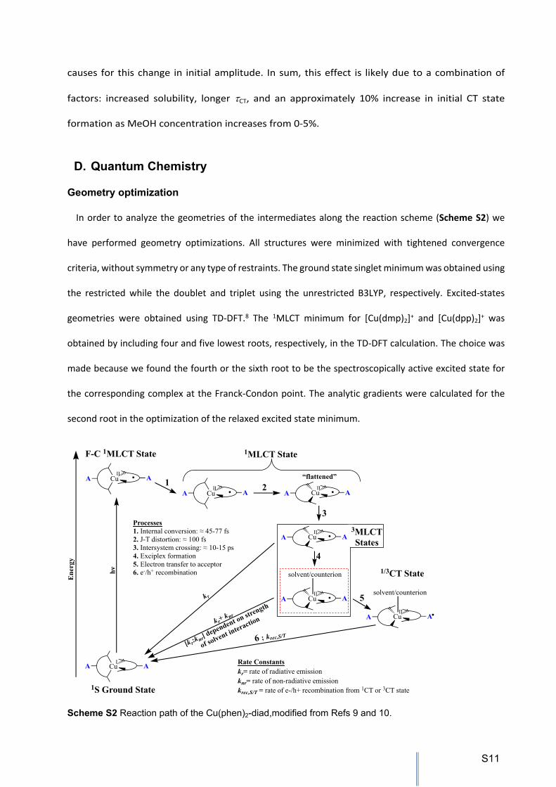
In order to analyze the geometries of the intermediates along the reaction scheme (Scheme S2) we

have performed geometry optimizations. All structures were minimized with tightened convergence

criteria, without symmetry or any type of restraints. The ground state singlet minimum was obtained using

the restricted while the doublet and triplet using the unrestricted B3LYP, respectively. Excited-states

geometries were obtained using TD-DFT.8 The 1MLCT minimum for [Cu(dmp)2]+ and [Cu(dpp)2]+ was

obtained by including four and five lowest roots, respectively, in the TD-DFT calculation. The choice was

made because we found the fourth or the sixth root to be the spectroscopically active excited state for

the corresponding complex at the Franck-Condon point. The analytic gradients were calculated for the

second root in the optimization of the relaxed excited state minimum.

Cu

CuI

II

1

hν

CuII

F-C 1MLCT State 1MLCT State

k r

k r+ knr

[k r:knr] dependent on strength

of solvent interaction

Ene

rgy

Processes1. Internal conversion: ≈ 45-77 fs2. J-T distortion: ≈ 100 fs3. Intersystem crossing: ≈ 10-15 ps4. Exciplex formation5. Electron transfer to acceptor6. e-/h+ recombination

• AA

AA

AA

•2Cu

II • AA

CuII

AA •

3

1S Ground State

4

“flattened”

CuII

AA •

solvent/counterion

3MLCTStates

CuII

AA •

solvent/counterion5

1/3CT State

6 ; krec,S/T

Rate Constantskr= rate of radiative emissionknr= rate of non-radiative emissionkrec,S/T = rate of e-/h+ recombination from 1CT or 3CT state

Scheme S2 Reaction path of the Cu(phen)2-diad,modified from Refs 9 and 10.

S11

Results of the geometry optimization

[Cu(dmp)2]+

The optimized ground state geometry of [Cu(dmp)2]+ shows D2d symmetry with considerable distortion

from tetrahedral geometry (Figure S6). The intraligand and interligand N-Cu-N bond angles are 82.4° and

124.5°, respectively. The dihedral angle between the two phen planes (θz) is 90° and all the Cu-N bonds

are identical with 2.044 Å (Table S1). Upon excitation the S3 state is populated, which is characterized by

a promotion of one electron from the dxz and dyz orbitals to a linear combination of π*-orbitals of the

ligand. Hence, this is a metal-to-ligand charge transfer (MLCT) state, which becomes apparent from the

difference density in Figure S7. This transition is dipole allowed and has the highest oscillator strength

(0.22) among the states within the visible range. The calculated vertical S0-S3 excitation energy of 2.6 eV

(21050 cm-1 (475 nm)) is in good agreement with the one deduced from the experimental absorption band

maximum at 22200 cm-1 (460 nm).11

Figure S6 Geometries of the dmp model. From the left to the right the minimum of the ground state, the lowest 1MLCT, the lowest 3MLCT and the doublet are shown.

Table S1 Geometrical parameters of the relaxed Cu(dmp)2 intermediates.

Parameter S01MLCT 3MLCT D0

bond lengths in ÅCu-N(1) 2.044 2.237 1.985 2.006Cu-N(10) 2.044 2.018 1.985 2.006Cu-N(1)’ 2.044 1.952 1.984 2.006

S12

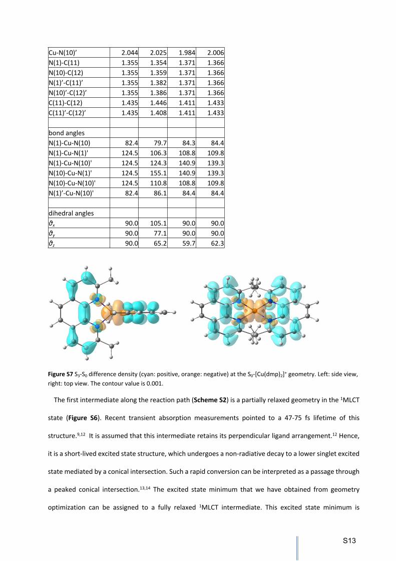
Cu-N(10)’ 2.044 2.025 1.984 2.006N(1)-C(11) 1.355 1.354 1.371 1.366N(10)-C(12) 1.355 1.359 1.371 1.366N(1)’-C(11)’ 1.355 1.382 1.371 1.366N(10)’-C(12)’ 1.355 1.386 1.371 1.366C(11)-C(12) 1.435 1.446 1.411 1.433C(11)’-C(12)’ 1.435 1.408 1.411 1.433

bond anglesN(1)-Cu-N(10) 82.4 79.7 84.3 84.4N(1)-Cu-N(1)' 124.5 106.3 108.8 109.8N(1)-Cu-N(10)' 124.5 124.3 140.9 139.3N(10)-Cu-N(1)' 124.5 155.1 140.9 139.3N(10)-Cu-N(10)' 124.5 110.8 108.8 109.8N(1)’-Cu-N(10)' 82.4 86.1 84.4 84.4

dihedral anglesθx 90.0 105.1 90.0 90.0θy 90.0 77.1 90.0 90.0θz 90.0 65.2 59.7 62.3

Figure S7 S3-S0 difference density (cyan: positive, orange: negative) at the S0-[Cu(dmp)2]+ geometry. Left: side view, right: top view. The contour value is 0.001.

The first intermediate along the reaction path (Scheme S2) is a partially relaxed geometry in the 1MLCT

state (Figure S6). Recent transient absorption measurements pointed to a 47-75 fs lifetime of this

structure.9,12 It is assumed that this intermediate retains its perpendicular ligand arrangement.12 Hence,

it is a short-lived excited state structure, which undergoes a non-radiative decay to a lower singlet excited

state mediated by a conical intersection. Such a rapid conversion can be interpreted as a passage through

a peaked conical intersection.13,14 The excited state minimum that we have obtained from geometry

optimization can be assigned to a fully relaxed 1MLCT intermediate. This excited state minimum is

S13

characterized by an oxidized d9-copper and a phen radical-anion. Such a singlet diradical character is

responsible for a difference in geometries of the two phen ligands because the excitation localizes at one

of the phen ligands. To understand the localization/delocalization pattern we have analyzed the

corresponding orbitals15 of a triplet diradical wave function (Figure S8). One singly occupied MO (SOMO)

is based on the dxz orbital of copper, while the other SOMO is of π*-type delocalized on the phen ligand.

From inspection of the latter it becomes apparent that N(1)’-C(11)’ and N(10)’-C(12)’ should be elongated

while C(11)’-C(12)’ should be shortened due to anti-bonding and bonding orbital lobes, respectively.

Indeed, these changes are confirmed by the geometrical parameters in Table S1. Furthermore, we find

shortened Cu-N bonds with 1.952 and 2.025 Å at the reduced phen ligand due to the formal 2+ charge of

Cu. The oxidation from d10 to d9-copper results also in a flattening of the phen ligands. The dihedral angle

θz between the two phen planes decreases from 90.0° to 62.3°. However, this distortion is accompanied

by significant rocking (θx of 105.1°) and wagging (θy of 77.1°) of the phen. All these changes are indicative

of a preferred five-coordinated copper in the d9 configuration. The next step of the reaction scheme leads

to a 3MLCT state through an intersystem crossing. The structurally relaxed 3MLCT intermediate is modeled

by a 3MLCT minimum geometry (Figure S6). The geometry of this model is characterized by four equal Cu-

N bonds and also both phen structures are identical, which is in line with the spin density in Figure S9.

Figure S8 Two SOMOs at the S1-[Cu(dmp)2]+ geometry. The contour value is 0.04.

S14

Figure S9 Spin density at the 3MLCT-[Cu(dmp)2]+ geometry. The contour value is 0.002.

In the last step of the reaction scheme (Scheme S2) an electron transfer from the ligand to the electron

acceptor takes place, which results in a weakly coupled diradical. In our study we model this intermediate

with [Cu(dmp)2]2+ in a doublet configuration. The Cu-N bonds of this model are shorter than those of the

singlet but slightly longer than those in the triplet. However, the geometry of phen ligand is nearly

unchanged from the ground state minimum. Finally, the spin density (Figure S10) clearly demonstrates an

unpaired electron in the d-orbital of copper. The Mulliken spin population at copper is 65%. The d9

configuration is responsible for a θz-value of 62.3° which is close to the singlet and triplet values. The

twisting between the phen planes is slightly increased as compared to the triplet geometry by 2.5°.

However, there is no rocking or wagging observed, as both θx- and θy-angles are 90° (Table S1).

Figure S10 Spin density at the D0-[Cu(dmp)2]2+ geometry. The contour value is 0.005.

[Cu(dpp)2]+

The optimized ground state structure of the [Cu(dpp)2]+ has D2 symmetry (Figure S11). It is characterized

by a 62° angle between the phen ligands. This flattening of the tetrahedral coordination is due to the steric

bulkiness of the phenyl substituents attached to the phen. We find an interligand π-stacking interaction

S15

between the phenyl and the phen with an off-center arrangement. Due to the π-π interaction the phenyl

rings are twisted by 39 degrees from the plane of the phen. Hence, this π-π interaction is more favorable

then the intraligand conjugation between the π-system of the phenyl and the phen. Besides the forced

flattening this particular geometry is also effectively shielding the Cu(I)-center from a possible

coordination by a MeOH solvent molecule as can be seen from the sphere representation of the D0-

structure in Figure S12. Thus, the geometry explains the lack of solvent dependence of Cu(dpp)2 in

contrast to Cu(dmp)2.

Figure S11 Geometries of the [Cu(dpp)2] model. From the left to the right the minimum of the ground, the lowest 1MLCT, the lowest 3MLCT and the doublet state are shown.

S16

Figure S12 Geometries of the doublet state with d9 Cu in a sphere representation. Left: [Cu(dmp)2]2+ model of MeC+A4

8+. Right: [Cu(dpp)2]2+ model of PhC+A48+.

The brightest excitation in the visible range of [Cu(dpp)2]+ is S0 S5 with an oscillator strength of 0.04.

It is dominated by a one-electron transition from the copper dxz based molecular orbital to a linear

combination of π*-orbitals of the phen ligand, as displayed in Figure S13 along with the difference density.

Due to the distortion of the phenyl out of the phen plane the density is mainly delocalized at the phen. In

addition also S1, S3 and S6 states have non-negligible oscillator strengths, while for [Cu(dmp)2]+ S3 is the

only bright state. This difference in absorption reflects the structural differences in the ground state. The

ground state geometry of [Cu(dpp)2]+ has D2 symmetry and is flattened already in contrast to higher

symmetry of the [Cu(dmp)2]+.

S17

Figure S13 Top: S5-S0 difference density (cyan: positive, orange: negative) at the S0-[Cu(dpp)2]+ geometry from two different perspectives. The contour value is 0.002. Bottom: HOMO (left) and LUMO (right) of [Cu(dpp)2]+. The contour value is 0.03.

An ultrafast decay is also observed for [Cu(dpp)2]+. This decay takes place within 125 fs16 which is slower

than in case of [Cu(dmp)2]+ but is still ultrafast, therefore precluding the formation of a minimum on the

S5 excited state. Hence, our optimization of the singlet excited state represents the relaxed 1MLCT

intermediate. The structural parameters collected in Table S2 show that the two phen ligands are

different. While at one phen-ligand the Cu-N bonds are shortened by 0.04 Å, they are lengthened at the

other phen-ligand by 0.07 Å. In addition, one ligand has a less pronounced conjugation displayed in the

N-C and the C(11)-C(12) bonds, while the other one is nearly unchanged as compared to the S0-geometry.

Further, the dihedral angle of the phenyl group from the phen residue is also different between the two

phen-ligands: 45° at phen and remaining 39° at phen’. These geometrical parameters point to the fact

that one phen is a radical anion carrying the electron from the copper. This becomes apparent from the

S18

inspection of the molecular orbitals: Figure S14 shows that the LUMO is a π*-orbital localized on only one

ligand. The shape of this LUMO explains also the reduced conjugation and in particular the shorter C(11)-

C(12) bond.

Figure S14 HOMO (left) and LUMO (right) at the S1-[Cu(dpp)2]+ geometry. The contour value is 0.03.

The oxidation of copper from d10 to d9 gives rise to a flattening of the complex which is of minor extent

compared to the Cu(dmp)2. The θz-angle decreases by 7° when going from S0 to S1 (Table S2). The next

relaxed intermediate, which is formed after the ISC is the optimized triplet model (Figure S11). It has

marginally shorter Cu-N and C(11)-C(12) bonds on one phen-ligand than on the other. There is also a

negligible difference of 1° in the phenyl-phen torsion between the two ligands. The spin density is found

on Cu and widely distributed on phen but not at the phenyl (Figure S15). Finally, the model of the CT state

resembles the trends observed for the [Cu(dmp)2]-complex. The Cu-N bonds are in-between those of the

singlet and triplet model. However, the phen geometry deviates slightly from the singlet case. The spin

density in Figure S16 affirms that the unpaired electron is residing on copper with a small contribution

from the adjacent N atoms.

Table S2 Geometrical parameters of the relaxed Cu(dpp)2 intermediates.

Parameter S01MLCT 3MLCT D0

bond lengths in ÅCu-N(1) 2.055 2.012 1.986 2.007Cu-N(10) 2.055 2.012 1.986 2.008Cu-N(1)’ 2.056 2.127 1.989 2.008

S19

Cu-N(10)’ 2.054 2.126 1.988 2.007N(1)-C(11) 1.356 1.379 1.370 1.360N(10)-C(12) 1.356 1.379 1.370 1.360N(1)’-C(11)’ 1.356 1.355 1.370 1.360N(10)’-C(12)’ 1.356 1.355 1.370 1.360C(11)-C(12) 1.446 1.411 1.421 1.434C(11)’-C(12)’ 1.446 1.444 1.422 1.434

bond anglesN(1)-Cu-N(10) 82.9 84.7 84.9 84.2N(1)-Cu-N(1)' 113.3 110.4 108.0 108.9N(1)-Cu-N(10)' 137.0 141.6 141.5 141.1N(10)-Cu-N(1)' 136.8 141.6 141.3 141.0N(10)-Cu-N(10)' 113.0 110.4 107.9 108.8N(1)’-Cu-N(10)' 82.9 79.9 84.9 84.2

dihedral anglesθx 90.0 90.0 90.0 89.9θy 90.2 90.0 90.1 90.1θz 67.4 59.8 58.7 59.7

phi 140.9 135.0 138.3 140.2140.6 135.2 137.9 140.2140.9 141.1 138.7 140.2140.6 141.0 138.8 140.2

Figure S15 Spin density at the 3MLCT-[Cu(dpp)2]+ geometry. The contour value is 0.002.

S20

Figure S16 Spin density at the D0-[Cu(dpp)2]2+ geometry. The contour value is 0.002.

Calculation of EPR parameters

In addition to the ab initio multireference calculations we have computed the g values and the hyperfine

coupling constants using DFT. For the DFT calculation of magnetic properties the same B3LYP functional

was used owing to its reasonable performance as documented in ref.17,18. To account for the relativistic

effect we have used the second-order Douglas-Kroll-Hess (DKH-2) transformation including the picture-

change effect.19 Especially for hyperfine coupling constants the use of DKH-2 operators instead of their

non-relativistic counterparts has been found to be crucial to obtain meaningful results.20 Further, we have

used a Gaussian finite-size nucleus model instead of a point charge model to take into account the

different extent of charge and magnetization distribution.20,21 The CP(PPP) basis set was adapted for

copper which is a more accurate triple-ξ basis with more flexibility in the core region. Hence, it is expected

that this choice will improve the Fermi contact contribution of the hyperfine coupling tensor. In addition,

larger integration grid in the radial part was chosen for copper to ensure accurate numerical integration

in the core region in the presence of very steep basis functions.22

The performance of B3LYP for the calculations of g values was evaluated for a number of copper

complexes. A systematic underestimation of the out of plane component by up to a factor of 2 was

observed and its origin has been rationalized.17 This underestimation leads to large errors in the

dominating value of the copper hyperfine coupling tensor, owing to the significantly lowered spin-orbit

component. To overcome this deficiency the correction shown in eq 1 involving the experimental Δg||

value was suggested by Sinnecker et al.:23

S21

(S1)A||(so)(corrected) A||

(so)(DFT) g||experimental

g||DFT

Such a correction was successfully applied to plastocyanin23 as well as type zero copper proteins.24 Hence,

we will also make use of this correction in the present study.

g-tensor

The theoretical g-values along with the directions of the principal axes of the g-tensor for [Cu(dmp)2]2+

and [Cu(dpp)2]2+, are given in Table S3 and Figures S17 and S18, respectively. For both complexes, the g3

principal axis is the unique molecular axis which bisects the largest of the N-Cu-N bond angles of 139.3°

in case of [Cu(dmp)2]2+ and 141.0° in case of [Cu(dpp)2]2+. For all methods, the g-matrix of [Cu(dpp)2]2+ is

found to be closer to axial symmetry than for [Cu(dmp)2]2+. The deviation between the g1 and g2 values at

the DFT level is 0.0004 for [Cu(dpp)2]2+ and 0.0087 for [Cu(dmp)2]2+. However, the deviation is larger at

the NEVPT2 level. At the SORCI level of theory, which is only available for the smaller [Cu(dmp)2]2+

complex, the deviation from axial symmetry is intermediate between that of DFT and NEVPT2.

While the experimental g value for [Cu(dpp)2]2+ is in quantitative agreement with the calculated g1 and

g2 values at the DFT level, the experimental g|| (g3) value is underestimated by as much as 0.18. The origin

of this 2-fold underestimation of the difference between g|| and g is widely recognized to be systematic

in DFT calculations.17 The QDPT approach with NEVPT2 energies yields a g|| value of 2.4547, which is in

better agreement with experiment, albeit somewhat too large. However, not only the g || value, but all g-

tensor components are overestimated. Compared to the experimental values, the g3 value is larger by

0.085, while g1, and g2 are overestimated by 0.005 and 0.0073, respectively. The systematically higher g-

tensor values might originate from the inconsistency of the CASSCF/NEVPT2 approach because the spin

orbit coupling (SOC) contribution is calculated using the SA-CASSCF wave function, while the denominator

in the QDPT expression utilizes NEVPT2 corrected energies. The SORCI method is more consistent due to

the equal treatment of SOC contribution and excitation energies, and it also recovers a larger part of the

differential dynamic correlation between the ground and the excited states in comparison to NEVPT2.

Thus, despite SORCI calculations being based on the same zeroth-order wave function as the NEVPT2, we

can expect the g values to be in better agreement with the experiment. The conceptual superiority of

S22

SORCI for g-tensor calculations was previously demonstrated for Cu(II) model complexes.25,26 However,

due to the large size of the [Cu(dpp)2]2+ complex a SORCI calculation was not feasible. Nevertheless, we

have studied the smaller complex [Cu(dmp)2]2+. As can be seen in Table S3, the differences of the g-tensor

components between the two complexes are below 0.008 at the DFT and at the CASSCF/NEVPT2 level of

theory. This small difference in the g tensor can be attributed to the approximate congruence of the CuN4

core in both complexes (see geometrical parameters in Tables S1 and S2). Hence, we can also expect that

the g-values of [Cu(dmp)2]2+ are very close to those of [Cu(dpp)2]2+ which justifies the comparison of the

SORCI results of the former with the experimental values of the latter. This comparison shows that SORCI

considerably improves the results: the calculated g3 value is only 0.012 higher than the experimental one

while g1 and g2 are 0.020 and 0.043 above the experimental values. It is gratifying to see this improvement,

considering that the difference of g values between the two complexes is of similar size as the deviation

between SORCI and the experimental values.

Table S3. Calculated g values for [Cu(dmp)2]2+ and [Cu(dpp)2]2+ models.

Model DFT NEVPT2 SORCI experiment 27

[Cu(dmp)2]2+

g1 (g,1) 2.0605 2.1173 2.0901

g2 (g,2) 2.0692 2.1502 2.1132

g3 (g||) 2.1891 2.4599 2.3827

giso 2.1062 2.2424 2.1953

[Cu(dpp)2]2+

g1 (g,1) 2.0668 2.1202 2.07

g2 (g,2) 2.0672 2.1434

g3 (g||) 2.1943 2.4547 2.37

giso 2.1095 2.2394

S23

Figure S17. Principal axes of the calculated g-tensor for the D0-[Cu(dmp)2]2+ structure.

Figure S18 Principal axes of the calculated g-tensor for the D0-[Cu(dpp)2]2+ structure. The hydrogens are left out for clarity.

Hyperfine coupling constants

The hyperfine coupling constants (HFC) for the copper in [Cu(dmp)2]2+ and [Cu(dpp)2]2+ are collected in

Table S4. We find the values similar for both complexes with a difference of only 2 MHz between the

isotropic A-value. This is in accordance with the similarity already observed for the g-tensor, due to the

nearly identical local coordination of the copper. The principal value A1 along the unique molecular axis

(Figures S19 and S20) is negative while the other two values are positive. Overall the HFC-tensor is nearly

axial which is again in line with the g-tensor analyzed above. Hence, in the following, the composition of

HFC can be discussed in general for both complexes.

The three contributions to the HFCs are the Fermi-contact term (fc), the spin dipolar contribution (sd),

and the spin-orbit term (so). In order to understand the change of sign for the principal values further

analysis is provided in Table S4. The total negative value of the HFCs can be traced back to the largely

negative A1 value. The decomposition of A1 reveals a negative A(fc) and A(sd) contribution while the A(so)

component is positive. The negative A(fc) term can be rationalized as a result of spin polarization induced

S24

by the unpaired electron at the copper. This spin polarization leads to a larger spin density of β- than α-

electrons. Such a “negative spin-density” is responsible for the negative sign. The A1 value is -16.7 mT for

[Cu(dpp)2]2+ which is in good agreement with the experimental value of A|| 17.7 MHz.27 Such a coincidence

with the experiment is due to fortunate error compensation from different contributions. The

underestimation g shift by the DFT is related to the spin-orbit contribution A(so). Hence, it is reflected in a

too small A(so) value. A simple scaling of this spin-orbit contribution is done to address this shortcoming:23,24

(S1)A||(so)(corrected) A||

(so)(DFT) g||experimental

g||DFT

Using the SORCI g|| shift for [Cu(dmp)2]2+ and the experimental value for [Cu(dpp)2]2+ results in a

scaling by a factor of 2. The corrected A|| values are -7.3 and -8.7 MHz for [Cu(dmp)2]2+ and [Cu(dpp)2]2+,

respectively. After the correction the agreement with experiment significantly worsens for the A|| value

of [Cu(dpp)2]2+. The largest deviation must come from the A||(fc) contribution.

In case of A2 and A3 a correction of the spin-orbit contribution is not necessary as the corresponding g

values are in good agreement with the experimental counterparts. In contrast to A1 the A(sd) contribution

becomes positive and of similar magnitude as A(fc). Hence, both A2 and A3 are positive. However, due to

its small size an experimental value could not be determined.

Table S4 Calculated Cu(II) A-tensor for [Cu(dmp)2]2+ and [Cu(dpp)2]2+ models in mT.

[Cu(dmp)2]2+ A1 (A||) A2 (A,1) A3 (A,2) Aiso

A(fc) -8.78 -8.78 -8.78

A(sd) -16.24 8.17 8.07

A(so) 8.74 (17.77)* 3.60 03.03

A(total) -16.27 (-7.28)* 03.00 02.32 -3.7 (-0.65)*

[Cu(dpp)2]2+

A(fc) -8.82 -8.82 -8.82

A(sd) -16.67 8.39 8.28

A(so) 8.78 (16.77)* 3.43 03.14

A(total) -16.70 (-8.71)* 03.00 02.61 -3.7 (-1.0)*

experiment27 17.7

S25

*corrected spin-orbit contribution after scaling is given in brackets.

Figure S19 Principal axes of the calculated A-tensor for the D0-[Cu(dmp)2]2+ structure.

Figure S20 Principal axes of the calculated A-tensor for the D0-[Cu(dpp)2]2+ structure.

The HFC tensors of nitrogen in [Cu(dmp)2]2+ and [Cu(dpp)2]2+ are given in Table S5. The coupling

constants are much smaller than those of copper, which is due to the lighter core, smaller polarization at

the core level and a negligible A(so) contribution (it is omitted from Table S5 because it is below 1

MHz=0.036 mT).18,28 Both complexes have four coordinating nitrogens which are expected to have

pairwise identical HFC tensors due to the D2 symmetry. However, we find a deviation below 0.05 MHz

(0.0018 mT) between the different nitrogen for each complex. Hence, we limit the discussion to one of

the nitrogens for each complex. Moreover, the differences between nitrogen’s HFC in [Cu(dmp)2]2+ and

[Cu(dpp)2]2+ are below 1 MHz (=0.036 mT). Hence, in the following we discuss results independent of the

complex. The A(fc) is the largest contribution to nitrogen’s HFC: 0.89-0.93 mT. Its value is positive in

contrast to the largely negative value in copper. This difference is not surprising because the nature of the

interaction is quite different: the isotropic contribution of nitrogen is dominated by the direct valence

S26

contribution, while in copper it is based on core-level spin-polarization.26 The A(sd) contribution is 0.21 to

0.25 mT for A|| and -0.11 to -0.14 mT for A. Since the spin-orbit contribution is below 1 MHz it can be

neglected and the total A|| and A values are 1.14 to 1.18 mT and 0.75 to 0.79 mT. Due to lack of

experimental data in the literature a comparison to measured HFC is not possible.

Table S5 Calculated 14N A-tensor for [Cu(dmp)2]2+ and [Cu(dpp)2]2+ models in mT.

[Cu(dmp)2]2+ A1 (A||) A2 (A,1) A3 (A,2) Aiso

A(fc) 0.93 0.93 0.93

A(sd) 0.25 -0.11

A(total) 1.18 0.82 0.79 0.89

[Cu(dpp)2]2+

A(fc) 0.89 0.89 0.89

A(sd) 0.21 -0.11 -0.14

A(total) 1.14 0.79 0.75 0.89

E. Theoretical calculation of CT decay time

Solving the set of differential equations (1) in the main text, in general yields a tri-exponential

function.

(S2)( ) exp( / ) exp( / ) exp( / )1 1 2 2 3 3f t A t A t A t

However, for the relevant range of kinetic parameters, the slowest of the exponential components re-

presents an amplitude fraction of more than 80 percent. To compare the theoretical with the

experimental results, an effective mono-exponential decay timeeff was determined by choosing eff such

that the integrated square deviation between the tri-exponential and the effective mono-exponential

curve was minimized. Thus, the following equation was obtained for eff

S27

(S3)( ) ( ) ( )

2 2 21 2 3

1 2 32 2 21 eff 2 eff 3 eff

1 04

A A A

which was solved numerically. The result thereby obtained was very close to one obtained by a simpler

relation, based upon the assumption that the time integrals over the tri-exponential and the effective

mono-exponential decay curves should be equal:

(S4)exp( / ) exp( / )

av0 0

i iA t dt t dt

This condition results in the equation

(S5) av i iA

In Figure S21 the resulting mono-exponential decay curves are shown for a set of characteristic field

values.

S28

B, mT

Figure S21 Quality of fit when replacing the tri-exponential decay by a mono-exponential one. The fields selected correspond to the data points marked in black in the fit of the experimental data shown in the first diagram in the center. Horizontal axis of the 6 decay traces: time, ns. Blue: tri-exponential decay, solid red: mono-exponential decay with decay time calculated by eq (S3) dashed red: mono-exponential decay with decay time calculated by eq (S5).

S29

F. Refined Analysis of McMillin Scheme

In a paper published in 1983 by McMillin and coworkers,29 the temperature dependence of emission

yield and life time of various copper(I) phenanthroline and bipyridine complexes were analyzed in terms

of an equilibrium between 1MLCT and 3MLCT state based on Scheme 3. Here we are extending this analysis

for the [Cu(dmp)2]+ complex making further use of experimental data published more recently,30 which is

discussed below.

1MLCT

3MLCT

kST

kTS

radiative partkf

total rate constant:

kS

total rate constant:

kT

radiative partkp

Scheme S3 Kinetic scheme describing MLCT state conversion and decay in Cu(I)(phen)2+ complexes according to

McMillin and coworkers.29

In the analysis in Ref.29 , it was assumed that the equilibrium between 1MLCT and 3MLCT is fully

established while observing the emission. However, since both the temperature dependent data of e and

e are given separately, the quantitative data analysis can be carried further without making the

assumption of a fully established ISC equilibrium. Recent fs-time-resolved experiments by Iwamura et al.31

have revealed that for 1MLCT photoexcited [Cu(dmp)2]+ the Jahn-Teller relaxation from D2d geometry,

where the two phenanthroline ligands are nearly perpendicular, to a flattened D2 geometry occurs within

about 0.8 ps, which is followed by a fast ISC process to 3MLCT within about 10 ps. The latter value is in

agreement with a previous observation by Siddique et al.30 and with more recent work by Castellano and

coworkers.32 That the quantum yield of prompt emission from 1MLCT corresponds to approximately 1/7

of the quantum yield of stationary emission represents an additional useful piece of information.30

S30

Based on the kinetic equations resulting from Scheme 3, the following relation can be derived.

(S6) e f p

TS T STf p

TS S ST T S T TS S ST T S T

k k kk kk k k k k k k k k k k k

where f denotes the yield of all quanta emitted from 1MLCT, p the yield of all quanta emitted from

3MLCT, kS and kT the overall decay constants of 1MLCT and 3MLCT, and kST and kTS the ISC rate constants

from 1MLCT to 3MLCT and vice versa, respectively.

The time dependent solution of formation and decay of 1MLCT and 3MLCT state is represented as a bi-

exponential function, with decay times in the 10 ps and the 100 ns range. Only the slower component was

measured in Ref.29. The analytical solution for the longer lifetime is given by

(S7) 12 2 2

e S T ST ST S ST ST S T ST T ST2 (1 ) ( ) 4 2( )( ) ( )k k k K k k k K k k k k K k k K

It can be adopted from the well know solution of excimer kinetics which is of the same type as Scheme 3.

As described by Kirchhoff et al.,29 the equilibrium constant K defined as

(S8)TS

ST

kKk

is calculated by

(S9)1 exp3

EKkT

with E describing the singlet/triplet energy gap. In their analysis, Kirchhoff et al.29 used the

approximation that the ratio T ST/k k is negligible in comparison to K. In that case, fitting the temperature

dependence of e e/ , yields kf and kp without any additional assumption. On the other hand, since an

experimental value of kST is known, the temperature dependence of e according to the exact eq(S7) can

be used to fit kT and kS, if these parameters and kST are assumed to be temperature independent in the

experimental range between 298 and 244 K (cf. Figure S22). With the kT value thus determined, and the

S31

experimental value of kST, eq (S6) to eq (S7) can be used for the fit of e e/ (cf. Figure S23) without

recourse to the approximation applied in Ref.29).

The temperature dependent fits were carried out with various values of E ranging between 1600

cm-1 and 1300 cm-1. McMillin and coworkers used a value of 1800 cm-1 but conceded a 20% uncertainty

for that value. Siddique et al.,30 based on spectral evidence and quantum chemical calculations, also

supported such a value of E. As follows from our analysis, such a value is not compatible with the set of

temperature dependent data on e and e given in Ref.29. Although the quality of the fits of e (T) and

e/e is hardly dependent on the value of E, the formal contribution of phosphorescence would turn to

negative values for E > 1653 cm-1. For the ratio of stationary to prompt fluorescence intensity, a marked

dependence on E is obtained. The fit parameter values to be selected for the various E are listed in

Table S6. The experimental ratio of about 1:7 is reproduced for E = 1350 cm-1.

e , ns

T, K

Figure S22 Fit of temperature dependent emission life time data for [Cu(dmp)2]+ from Kirchhoff et al.29 using equation (S7). Blue curve for E = 1350 cm-1 with kS = 4.97 ns-1 and kT = 0.0092 ns-1; red curve for E = 1600 cm-1 with kS = 17.2 ns-1 and kT = 0.0094 ns-1.

S32

4e e10 /

T, KFigure S23 Fitting kf and kp to simulate the temperature dependence of e/e using equations (S6) to (S9)with E =

1350 cm-1. The best fit values are kf = 3.0106 s-1 and kp = 7.0102 s-1. For values of other parameters cf. Table S6.

S33

Table S6 Parameter values and quantum yields(a) based on best fits of [T] and [T], assuming kST = 100 ns-1 and kA = 3.2 ns-1.

E 1/K[24,1oC] kS kT kf kp f,prompt f p e e/f,prompt CT %1CTcm-1 ns-1 ns-1 ns-1 ns-1 10-4 10-4 10-4 10-4 %1600 7007 17.2 0.0094 0.0104 2.51×10-7(b) 0.89 1.83 0.19 2.01 2.27 0.85 3.1

1400 2657 6.30 0.0092 0.0038 6.64×10-7 0.36 1.46 0.55 2.01 5.61 0.94 3.1

1360 2191 5.21 0.0092 0.0031 6.93×10-7 0.30 1.43 0.58 2.00 6.72 0.95 3.2

1350 2085 4.97 0.0092 0.0030 6.99×10-7 0.29 1.42 0.58 2.01 7.03 0.95 3.2

1300 1637 3.94 0.0091 0.0024 7.18×10-7 0.23 1.40 0.60 2.00 8.78 0.96 3.2

(a) The various quantum yields refer to prompt emission (f,prompt), total emission from 1MLCT (f), total emission from 3MLCT (p), total emission (e). The quantum yield of CT-state formation on reaction with an appended acceptor is denoted CT, of which a percentage %1CT is formed with singlet spin multiplicity. All quantum yields refer to 24.1oC. (b)The contribution of phosphorescence drops to zero if E ≈ 1653 cm-1 and becomes formally negative for higher values.

S34

S35

G. Emission decay curves

Figure S24 Emission decay curves for PhC+A48+ (upper panel) and MeC+A4

8+ (lower panel) with tri-exponential fit curves and residuals. The decay times are 0.32 ns (84%), 1.25 ns (15%) and 10.3 ns (1%) in case of PhC+A4

8+ and 0.22 ns (25%), 1.23 ns (51%) and 4.13 ns (24%) in case of MeC+A4

8+

It is assumed that the multi-exponential decay results from an inhomogeneity of the emissive species

concerning the conformations of the side arms and/or association with counter ions (cf. RESULTS in the

main text).

S36

H. Spin motion and spin relaxation

Spin relaxation

Within the Redfield approach, the following equations are valid for electron spin relaxation due to

rotational modulation of an anisotropic g-tensor and of anisotropic hyperfine coupling to a nuclear spin33

(S10) 2 2 2 2

0 0 2 21 0

1 1 27 1 420 3 1

rN N I I

r

A I I m m A g gT

(S11)

2 2 2 20 0

2 2 2 220 0 2 2

0

1 2 13 1 58 3 91 1

5 1 1 17 18 2 12 1

N N I I r

rN N I I

r

A I I m m A g g

T A I I m m A g g

Here IN is the quantum number of total nuclear spin and mI the magnetic axial quantum number, is A

the hyperfine anisotropy in frequency units:

(S12)( )eA A A P

with e the gyromagnetic ratio of the electron, the g-tensor anisotropyg

(S13)g g g P

and 0 the Larmor frequency. The rotational correlation time r can be estimated by the Debye-Einstein

equation

(S14)34r R

kT

with the solvent viscosity and R the effective hydrodynamic radius of the complex. For difluorobenzene,

the viscosity at room temperature was determined as 0.6210-3 Pas.

The effective hydrodynamic radius can be estimated by relating the Connolly surface of the complex

into the radius of a sphere.34 The Connolly surface obtained by Chem3D pro 14.1 from the structure given

in Figure 7 of the main text amounts to 1360 Å2 yielding an effective radius R of 10.4 Å. From these data

a value of 0.71 ns is obtained forr.

S37

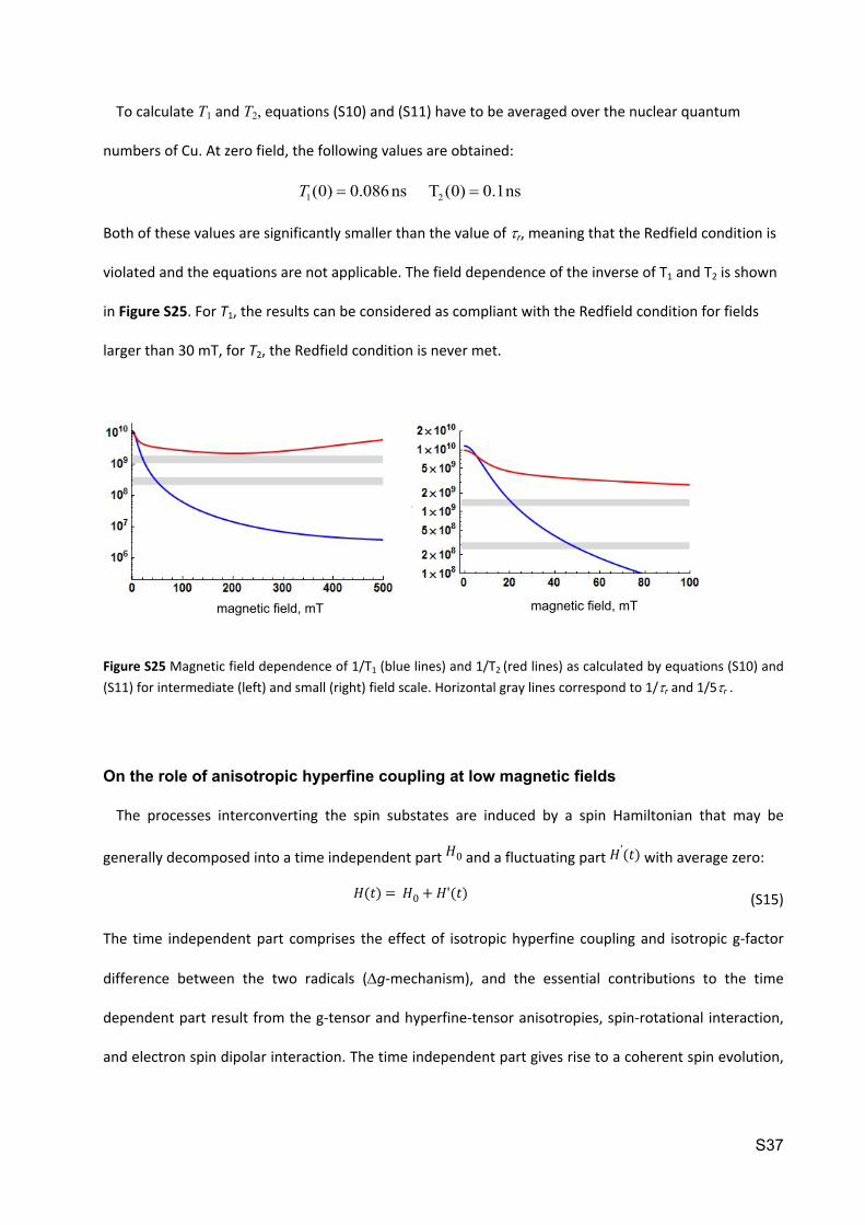
To calculate T1 and T2, equations (S10) and (S11) have to be averaged over the nuclear quantum

numbers of Cu. At zero field, the following values are obtained:

1 2(0) 0.086ns T (0) 0.1nsT

Both of these values are significantly smaller than the value of r, meaning that the Redfield condition is

violated and the equations are not applicable. The field dependence of the inverse of T1 and T2 is shown

in Figure S25. For T1, the results can be considered as compliant with the Redfield condition for fields

larger than 30 mT, for T2, the Redfield condition is never met.

magnetic field, mTmagnetic field, mT

Figure S25 Magnetic field dependence of 1/T1 (blue lines) and 1/T2 (red lines) as calculated by equations (S10) and (S11) for intermediate (left) and small (right) field scale. Horizontal gray lines correspond to 1/r and 1/5r .

On the role of anisotropic hyperfine coupling at low magnetic fields

The processes interconverting the spin substates are induced by a spin Hamiltonian that may be

generally decomposed into a time independent part and a fluctuating part with average zero: 𝐻0 𝐻'(𝑡)

(S15)𝐻(𝑡) = 𝐻0 + 𝐻'(𝑡)

The time independent part comprises the effect of isotropic hyperfine coupling and isotropic g-factor

difference between the two radicals (g-mechanism), and the essential contributions to the time

dependent part result from the g-tensor and hyperfine-tensor anisotropies, spin-rotational interaction,

and electron spin dipolar interaction. The time independent part gives rise to a coherent spin evolution,

S38

strictly to be described by explicit quantum dynamics. If the correlation times of the fluctuations

modulating are sufficiently short to fulfil the Redfield condition𝐻'(𝑡)

(S16)𝜏𝑐 ≪ 𝑇1,𝑇2

where τc is the correlation time of the fluctuation and T1 and T 2 are the relaxation times obtained by

second order time-dependent perturbation theory, the pertinent effects can be reliably described by

incoherent relaxation processes with these time constants. The most important source of fluctuating

interactions in liquid solution is molecular tumbling, which modulates the effects of g-tensor and

hyperfine tensor anisotropies and of electron spin dipolar interaction. Furthermore, it may give rise to

spin-rotational coupling. Specific equations for the pertinent relaxation times are available in the

literature and have been used to test condition (S16). The correlation times to be considered are the

rotational correlation time, R, and the correlation time of angular momentum,. These are given by the

following expressions:35

(S17)𝜏𝑅 =

4𝜋𝜂3𝑘𝑇

𝑅3

and (S18)𝜏𝜔 =

𝜃

8𝜋𝜂𝑅3

where is the solvent viscosity, R the molecular hydrodynamic radius, and the molecular moment of

inertia. Substituting the specific values of solvent and MeC+A48+ complex, = 0.62 mPa s, 2.03×10-42 kg

m2 and R 10.4 Å. one can estimate the values 0.71 ns and 0.12 p s. When the anisotropic 𝜏𝑅 𝜏𝜔

hyperfine interaction is modulated, the rotational motion of the complex is too slow to comply with

condition (S16). For T1 at fields below 30 mT and for T2 at any field, this is a consequence of the strong

anisotropy of the Cu hyperfine coupling, and rather exceptional in the field of spin chemistry.36 It means

that, in a correct sense, this anisotropy would have to be taken into account on the time scale of explicit

quantum dynamics under conditions of slow molecular tumbling. A full treatment of that kind is beyond

the scope of the present work. As an approximation, we will use a modified value of the isotropic hyperfine

coupling which will be introduced as an empirical parameter. Since the same type of Lorentzian field

dependence as assumed for the coherent mixing process does apply to spin relaxation due to anisotropic

S39

hyperfine coupling (cf. eq (9) in the main text ), the Lorentzian approach also includes incoherent

contributions in the field regions where condition (S16) does apply. Here coherent and incoherent

contributions are indistinguishable. In the case of spin-rotational interaction, which yields a sizeable

contribution, condition (S16) is well satisfied by the value of 𝜏𝜔.

Moment of inertia

The moment of inertia of [Cu(Me4OMV)]9+ was calculated from the geometry shown in Figure 7 of the

main text, using the definition of the elements of the tensor of inertia

(S19) 2kl lk i i kl ik il

iI I m r x x

where mi represents the mass of atom i, ri its radial position, and the xik its Cartesian coordinates, the

indices k and l running over the three dimensions x, y, z. The principle moments of inertia are obtained

by diagonalization of this tensor:

211

222

233=175462 , =166930u , =62464 u 5 uÅ Å Å

yielding a geometric average of .2 42 2u 2.03..12230 10 kg m7 Å

S40

Estimation of classical rate constants representing coherent mixing processes

S/T0 mixing by g-mechanism

For isotropically averaged g-tensors, the Zeeman Hamiltonian of a radical pair is given by

(S20)1 0 1 2 0 2Z B z B zH g B S g B S

It mixes the radical pair state |S> and |T0> by the matrix element

(S21)0 012ZS H T g B

Then the coherent evolution of singlet probability, when starting from a pure |T0> is given by

(S22) ,

1( ) 1 cos( )2S cohp t t

with given by

(S23)0g B

The function is shown in Figure S26𝑝𝑆(𝑡)

Figure S26 Time dependence of singlet probability for a pure |T0> function at t = 0. Blue: coherent motion according to the g-mechanism. Red: exponential approach to equilibrium according to the kinetic model. The rate constant

is chosen such as to yield equal areas F1 and F2.𝑘∆𝑔

The classical kinetic equilibration between S and T0 is described by the kinetic scheme

(S24)0S Tg

g

k

k

It leads to the following kinetics of equilibration:

S41

(S25) ,1 1 exp 22S kin gp k t

For matching the classical with the quantum kinetics, one may assume that the time integrals over

before the crossing point of both curves and after the crossing , ,S coh S kinp p, ,

1,2S coh S kinMin p p

point for < 3/2 plus the time integral over for t 3/2 (cf. shaded areas in Figure S26) t ,12 S kinp

are equal. This leads to the equation

(S26)12gk

General S/T0 mixing and S/T and T0/T mixing in zero field by isotropic hfc

If we assume the following classical kinetic schemes for zero field

(S27)

0

0

S T ,

S T

T T

hfc

hfc

hfc

hfc

hfc

hfc

k

k

k

k

k

k

and high field

(S28)0S T ,hfc

hfc

k

k

and we start with an equal population of the triplet states, the evolution of the singlet population is as

follows. At zero field

(S29) , ,01( ) 1 exp 44S zF hfcp t k t

and at high field

(S30) , ,01( ) 1 exp 26S hF hfcp t k t

We will compare the resulting behavior with the semiclassical spin motion for zero field and high field as

derived by Schulten and Wolynes37 According to these authors the isotropic hyperfine coupling situation

in each radical is reduced to a characteristic time constant I by the relation

S42

(S31)22

1 1 ( 1)6 ik ik ik

i

a I I

In zero field the singlet probability of an initial triplet radical pair is given by

(S32) , 1 21 11 1 2 ( / ) 1 2 ( / )4 9S zFp f t f t

with the definition

(S33)2 2( ) (1 2 )exp( )f x x x

In high field, the result is

(S34) 2 2 2 2, 1 2

1( ) 1 exp / exp /6S hFp t t t

In eq (S35) the two individual time constants can be contracted to a single one by using the definition

(S35)2 2 2

1 2

1 1 1

With this definition, eq (S35) is simplified to

(S36) 2 2,

1( ) 1 exp /6S hFp t t

It may be of interest to relate the characteristic time constants to the characteristic fields 1 2, , and

B1, B2, and B1/2 used in the spin chemical literature.38 The relations are:

(S37) 1/22 ( 1)ik ik ki ia IB I kl

Hence

(S38)6

iiB

kl

The simplest relation between B1, B2, and B1/2 is39

(S39)2 2 21/2 1 23( )B B B kl

Hence

S43

(S40)1/2

3 2B

In Figure S27 the various functions of are shown for the specific example of the Cu(Mephen)2+..MV2+ ( )Sp t

radical pair. If one chooses khfc,0 in the classical kinetics description by the criterion that for the high-field

curve the integrals over classical and semiclassical curves should be equal, one can derive the relation

(S41)1/2,0

13 2hfc

Bk

which does not depend on the individual values i or Bi of the two radicals.

Sp

t,ns

Figure S27 Spin motion due to isotropic hyperfine coupling. Solid curves: semi-classical model for radical pair (Cu(Mephen)2

+..MV2+ B1 = 78 G , B2 = 12.5 G, B1/2 = 137 G). Blue: zero field, red: high field. Dashed curves: classical kinetics (eqs. (S29) and S(39)). The rate constant khfc,0 = 3.2108 s-1 was chosen such that the two shaded areas between the classical and the semi-classical high field curves became equal.

Advanced semiclassical theory

The semiclassical approach to hyperfine controlled spin motion in radical pairs by Schulten and

coworkers37,40 has recently been extended by Lewis, Manolopoulos and Hore.41,42 In these advanced

versions, each nuclear spin vector is allowed to precess independently around the electron spin vector

S44

whereas in the original versions a hyperfine weighted sum of nuclear spins was used. Furthermore, the

method has been extended to account for different reactivity of singlet and triplet.

The authors of ref. 42 kindly provided us with a program code to apply the extended semiclassical theory

to our system.

The following hyperfine constants have been used: Cu: I = 3/2, a = -4,0 mT, MV+: 4×aH= 0.134 mT, 4×aH=

0.159 mT, 6×aH= 0.401 mT.

First, we calculated the hyperfine induced spin motion without reaction (cf. Figure S28 to compare it

with the result obtained by the Schulten method.

Figure S28 Semiclassical spin motion, evolution of singlet character in a Cu(II)/MV+ radical pair, when starting in a pure triplet. Blue: zero field, red. High field limit. The dashed lines correspond to classical kinetics with kTS0 = 3.8 x 108 s-1.Left: Coherent spin motion according to Lewis et al.42 right: according to Schulten and Wolynes.37 Both diagrams show the same classical kinetics curves.

In the more advanced calculations, the spin motion shows stronger oscillations, but the purely

exponential substitutes we used in our classical kinetics model fits the more advance model even better.

For the full treatment, including reaction, a field dependent parametrization of spin relaxation times

must be provided for the advanced semiclassical model. To this end, we took the spin relaxation times

following from our treatment. The field dependent values of the relaxation times (only the Cu(II) complex

was considered) were obtained by the following equations, based on eqs. (2), (7) and (8) in the main

paper:

(S42)0 02

1 2( [ ] )' TS hfck B k

T

S45

(S43)11

1 4( [ ] [ ])hfck B k BT

(S44)2 2 1

1 1 1' 2T T T

Thus, we made sure that the classical treatment in our paper and the advanced semiclassical treatment

differed only in the way the effect of hyperfine coupling was dealt with, while employing the same

contributions of spin relaxation.

The g effect was implicitly taken into account through the value of relaxation time T2’ of the Cu(II)

complex.

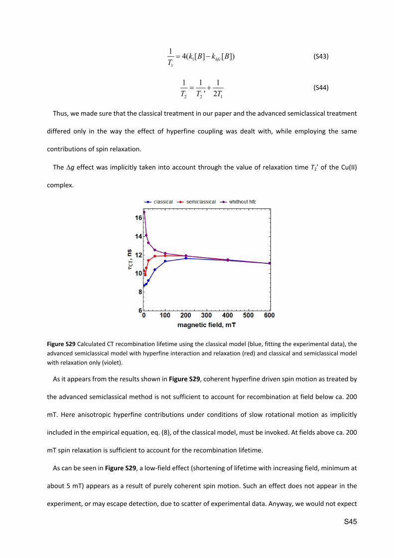
Figure S29 Calculated CT recombination lifetime using the classical model (blue, fitting the experimental data), the advanced semiclassical model with hyperfine interaction and relaxation (red) and classical and semiclassical model with relaxation only (violet).

As it appears from the results shown in Figure S29, coherent hyperfine driven spin motion as treated by

the advanced semiclassical method is not sufficient to account for recombination at field below ca. 200

mT. Here anisotropic hyperfine contributions under conditions of slow rotational motion as implicitly

included in the empirical equation, eq. (8), of the classical model, must be invoked. At fields above ca. 200

mT spin relaxation is sufficient to account for the recombination lifetime.

As can be seen in Figure S29, a low-field effect (shortening of lifetime with increasing field, minimum at

about 5 mT) appears as a result of purely coherent spin motion. Such an effect does not appear in the

experiment, or may escape detection, due to scatter of experimental data. Anyway, we would not expect

S46

it to occur if anisotropic hyperfine interactions under rotational slow-motion conditions did contribute to

spin evolution.

Supplementary Diagrams

magnetic field, mT

CT, ns

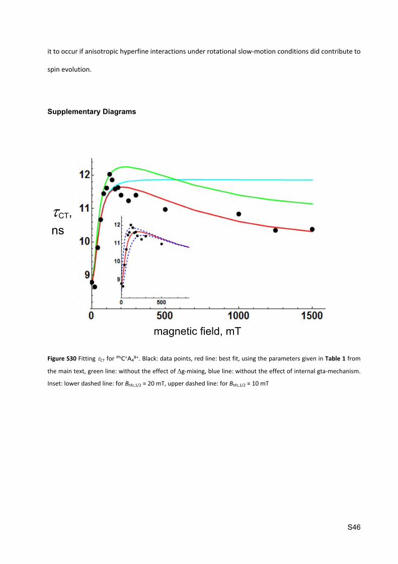
Figure S30 Fitting CT for PhC+A48+. Black: data points, red line: best fit, using the parameters given in Table 1 from

the main text, green line: without the effect of g-mixing, blue line: without the effect of internal gta-mechanism.

Inset: lower dashed line: for Bhfc,1/2 = 20 mT, upper dashed line: for Bhfc,1/2 = 10 mT

S47

magnetic field, mT

CT

,

ns

Figure S31 Data points: lifetime of charge separated state for MeC+A48+ in dfb. Red curve: simulation using the

parameters given in Table 1 of the main text.

Figure S32 Magnetic field dependence of various contributions to spin dynamics and related parameters for MeC+A48+

in pure dfb. Red data points: inverse of experimental CT values with best fit line from Figure S31 in black.

S48

magnetic field, mT

CT

,

ns

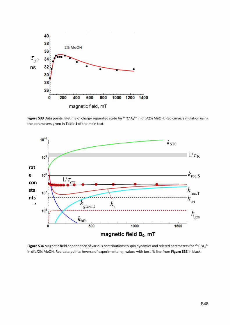
Figure S33 Data points: lifetime of charge separated state for MeC+A48+ in dfb/2% MeOH. Red curve: simulation using

the parameters given in Table 1 of the main text.

rate constants, s-1

magnetic field B0, mT

kST0

1/ R

krec,S

krec,T

kgta-int

ksri

khfc

k±

1/CT

kgta

Figure S34 Magnetic field dependence of various contributions to spin dynamics and related parameters for MeC+A48+

in dfb/2% MeOH. Red data points: inverse of experimental CT values with best fit line from Figure S33 in black.

S49

magnetic field, mT

CT

,

ns

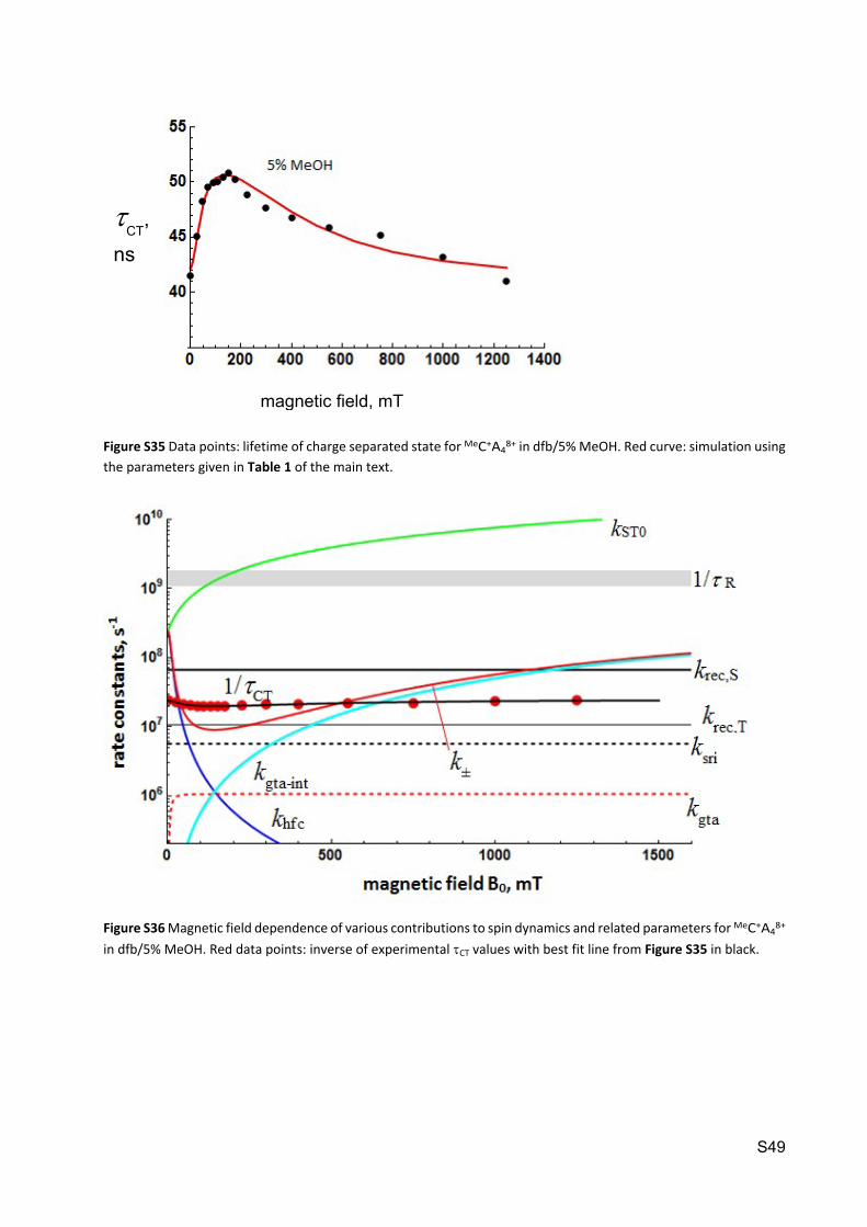
Figure S35 Data points: lifetime of charge separated state for MeC+A48+ in dfb/5% MeOH. Red curve: simulation using

the parameters given in Table 1 of the main text.

Figure S36 Magnetic field dependence of various contributions to spin dynamics and related parameters for MeC+A48+

in dfb/5% MeOH. Red data points: inverse of experimental CT values with best fit line from Figure S35 in black.

S50

magnetic field, mT

CT

,

ns

Figure S37 Data points: lifetime of charge separated state for MeC+A48+ in dfb/10% MeOH. Red curve: simulation

using the parameters given in Table 1 of the main text.

Figure S38 Magnetic field dependence of various contributions to spin dynamics and related parameters for MeC+A48+

in dfb/10% MeOH. Red data points: inverse of experimental CT values with best fit line from Figure S37 in black.

S51

I. References

1 J. Hong, M. P. Shores and C. M. Elliott, Inorg. Chem., 2010, 49, 11378–11385.2 F. Calderazzo, F. Marchetti, G. Pampaloni and V. Passarelli, J. Chem. Soc. Dalt. Trans.,

1999, 4389–4396.3 A. M. S. Garas and R. S. Vagg, J. Heterocycl. Chem., 2000, 37, 151–158.4 N. Margiotta, V. Bertolasi, F. Capitella, L. Maresca, A. G. G. Moliterni, F. Vizza and G.

Natile, Inorganica Chim. Acta, 2004, 357, 149–158.5 A. P. Lehnig, M. S. Lazorski, M. Mingroni, K. A. O. Pacheco and C. Michael Elliott, J.

Heterocycl. Chem., 2014, 51, 1468–1471.6 J.-Z. Wu, H. Li, J.-G. Zhang and J.-H. Xu, Inorg. Chem. Commun., 2002, 5, 71–75.7 M. L. Rizzo, Statistical Computing with R, CRC Press, Boca Raton, 2007.8 T. Petrenko, S. Kossmann and F. Neese, J. Chem. Phys., 2011, 134, 054116.9 G. B. Shaw, C. D. Grant, H. Shirota, E. W. C. Jr, G. J. Meyer and L. X. Chen, J. Am.

Chem. Soc., 2007, 129, 2147–2160.10 D. V Scaltrito, D. W. Thompson, J. a O’Callaghan and G. J. Meyer, Coord. Chem. Rev.,

2000, 208, 243–266.11 A. K. Ichinaga, J. R. Kirchhoff, D. R. McMillin, C. O. Dietrich-Buchecker, P. A. Marnot and

J. P. Sauvage, Inorg. Chem., 1987, 26, 4290–4292.12 M. Iwamura, S. Takeuchi and T. Tahara, J. Am. Chem. Soc., 2007, 129, 5248–5256.13 G. J. Atchity, S. S. Xantheas and K. Ruedenberg, J. Chem. Phys., 1991, 95, 1862–1876.14 T. J. Martinez, Nature, 2010, 467, 412–413.15 F. Neese, J. Phys. Chem. Solids, 2004, 65, 781–785.16 M. Iwamura, S. Takeuchi and T. Tahara, Phys. Chem. Chem. Phys., 2014, 16, 4143–

4155.17 F. Neese, J. Chem. Phys., 2001, 115, 11080.18 F. Neese, J. Chem. Phys., 2003, 118, 3939.19 B. Sandhoefer and F. Neese, J. Chem. Phys., 2012, 137, 094102.20 B. Sandhoefer, S. Kossmann and F. Neese, J. Chem. Phys., 2013, 138, 104102.21 L. Visscher and K. G. Dyall, At. Data Nucl. Data Tables, 1997, 67, 207–224.22 F. Neese, Inorganica Chim. Acta, 2002, 337, 181–192.23 S. Sinnecker and F. Neese, J. Comput. Chem., 2006, 27, 1463–75.24 K. M. Lancaster, M.-E. Zaballa, S. Sproules, M. Sundararajan, S. DeBeer, J. H. Richards,

A. J. Vila, F. Neese and H. B. Gray, J. Am. Chem. Soc., 2012, 134, 8241–53.25 S. Vancoillie, P.-A. Malmqvist and K. Pierloot, Chemphyschem, 2007, 8, 1803–15.26 F. Neese, Magn. Reson. Chem., 2004, 42 Spec no, S187-98.27 M. T. Miller, P. K. Gantzel and T. B. Karpishin, Inorg. Chem., 1998, 37, 2285–2290.28 F. Neese, J. Phys. Chem. A, 2001, 105, 4290–4299.29 J. R. Kirchhoff, R. E. Gamache, M. W. Blaskie, A. A. D. Paggio, R. K. Lengel and D. R.

McMillin, Inorg. Chem., 1983, 22, 2380–2384.30 Z. A. Siddique, Y. Yamamoto, T. Ohno and K. Nozaki, Inorg. Chem., 2003, 42, 6366–78.

S52

31 M. Iwamura, H. Watanabe, K. Ishii, S. Takeuchi and T. Tahara, J. Am. Chem. Soc., 2011, 133, 7728–7736.

32 S. Garakyaraghi, E. O. Danilov, C. E. McCusker and F. N. Castellano, J. Phys. Chem. A, 2015, 119, 3181–3193.

33 L. Banci, I. Bertini and C. (Claudio) Luchinat, Nuclear and electron relaxation, VCH Publishers Inc., New York, 1991.

34 J. H. Klein, D. Schmidt, U. E. Steiner and C. Lambert, J. Am. Chem. Soc., 2015, 137, 11011–11021.

35 P. W. Atkins and D. Kivelson, J. Chem. Phys., 1966, 44, 169.36 Note: In [Ru(bpy)3]3+ the g-tensor anisotropy is quite high, but in radical pairs involving

that species the dominating spin conversion mechanism is spin relaxation by the rotation-independent Orbach mechanism (cf. K. A. Hötzer, A. Klingert, T. Klumpp, E. Krissinel, D. Bürßner, and U. E. Steiner, J. Phys. Chem. A., 2002, 106, 2207-2217).

37 K. Schulten and P. G. Wolynes, J. Chem. Phys., 1978, 68, 3292.38 A. Weller, F. Nolting and H. Staerk, Chem. Phys. Lett., 1983, 96, 24–27.39 U. E. Steiner and H. J. Wolff, in Photochemistry and Photophysics, eds. J. J. Rabek and

G. W. Scott, CRC Press, Boca Raton, 1991, vol. IV, pp. 1–130.40 E.-W. Knapp and K. Schulten, J. Chem. Phys., 1979, 71, 1878.41 D. E. Manolopoulos and P. J. Hore, J. Chem. Phys., 2013, 139, 124106 (1–8).42 A. M. Lewis, D. E. Manolopoulos and P. J. Hore, J. Chem. Phys., 2014, 141, 44111.