support vector machines: theory and applications · preface the support vector machine (svm) is a...

Support Vector Machines: Theory and Applications

Lipo Wang

(ed.)

Springer, Berlin

2005

Preface

The support vector machine (SVM) is a supervised learning method thatgenerates input-output mapping functions from a set of labeled training data.The mapping function can be either a classification function, i.e., the cate-gory of the input data, or a regression function. For classification, nonlinearkernel functions are often used to transform input data to a high-dimensionalfeature space in which the input data become more separable compared tothe original input space. Maximum-margin hyperplanes are then created. Themodel thus produced depends on only a subset of the training data near theclass boundaries. Similarly, the model produced by Support Vector Regres-sion ignores any training data that is sufficiently close to the model prediction.SVMs are also said to belong to “kernel methods”.

In addition to its solid mathematical foundation in statistical learningtheory, SVMs have demonstrated highly competitive performance in numerousreal-world applications, such as bioinformatics, text mining, face recognition,and image processing, which has established SVMs as one of the state-of-the-art tools for machine learning and data mining, along with other softcomputing techniques, e.g., neural networks and fuzzy systems.

This volume is composed of 20 chapters selected from the recent myriadof novel SVM applications, powerful SVM algorithms, as well as enlighten-ing theoretical analysis. Written by experts in their respective fields, the first12 chapters concentrate on SVM theory, whereas the subsequent 8 chaptersemphasize practical applications, although the “decision boundary” separat-ing these two categories is rather “fuzzy”.

Kecman first presents an introduction on the SVM, explaining the basictheory and implementation aspects. In the chapter contributed by Ma andCherkassky, a novel approach to nonlinear classification using a collection ofseveral simple (linear) classifiers is proposed based on a new formulation ofthe learning problem called multiple model estimation. Pelckmans, Goethals,De Brabanter, Suykens, and De Moor describe componentwise Least SquaresSupport Vector Machines (LS-SVMs) for the estimation of additive modelsconsisting of a sum of nonlinear components.

VI Preface

Motivated by the statistical query model, Mitra, Murthy and Pal study anactive learning strategy to solve the large quadratic programming problem ofSVM design in data mining applications. Kaizhu Huang, Haiqin Yang, King,and Lyu propose a unifying theory of the Maxi-Min Margin Machine (M4)that subsumes the SVM, the minimax probability machine, and the lineardiscriminant analysis. Vogt and Kecman present an active-set algorithm forquadratic programming problems in SVMs, as an alternative to working-set(decomposition) techniques, especially when the data set is not too large, theproblem is ill-conditioned, or when high precision is needed.

Being aware of the abundance of methods for SVM model selection,Anguita, Boni, Ridella, Rivieccio, and Sterpi carefully analyze the most well-known methods and test some of them on standard benchmarks to evaluatetheir effectiveness. In an attempt to minimize bias, Peng, Heisterkamp, andDai propose locally adaptive nearest neighbor classification methods by usinglocally linear SVMs and quasiconformal transformed kernels. Williams, Wu,and Feng discuss two geometric methods to improve SVM performance, i.e.,(1) adapting kernels by magnifying the Riemannian metric in the neighbor-hood of the boundary, thereby increasing class separation, and (2) optimallylocating the separating boundary, given that the distributions of data on eitherside may have different scales.

Song, Hu, and Xulei Yang derive a Kuhn-Tucker condition and a decom-position algorithm for robust SVMs to deal with overfitting in the presence ofoutliers. Lin and Sheng-de Wang design a fuzzy SVM with automatic deter-mination of the membership functions. Kecman, Te-Ming Huang, and Vogtpresent the latest developments and results of the Iterative Single Data Algo-rithm for solving large-scale problems.

Exploiting regularization and subspace decomposition techniques, Lu,Plataniotis, and Venetsanopoulos introduce a new kernel discriminant learn-ing method and apply the method to face recognition. Kwang In Kim, Jung,and Hang Joon Kim employ SVMs and neural networks for automobile li-cense plate localization, by classifying each pixel in the image into the objectof interest or the background based on localized color texture patterns. Mat-tera discusses SVM applications in signal processing, especially the problemof digital channel equalization. Chu, Jin, and Lipo Wang use SVMs to solvetwo important problems in bioinformatics, i.e., cancer diagnosis based on mi-croarray gene expression data and protein secondary structure prediction.

Emulating the natural nose, Brezmes, Llobet, Al-Khalifa, Maldonado, andGardner describe how SVMs are being evaluated in the gas sensor commu-nity to discriminate different blends of coffee, different types of vapors andnerve agents. Zhan presents an application of the SVM in inverse problemsin ocean color remote sensing. Liang uses SVMs for non-invasive diagnosisof delayed gastric emptying from the cutaneous electrogastrograms (EGGs).Rojo-Alvarez, Garcıa-Alberola, Artes-Rodrıguez, and Arenal-Maız applySVMs, together with bootstrap resampling and principal component analysis,to tachycardia discrimination in implantable cardioverter defibrillators.

Preface VII

I would like to express my sincere appreciation to all authors and reviewerswho have spent their precious time and efforts in making this book a reality.I wish to especially thank Professor Vojislav Kecman, who graciously tookon the enormous task of writing a comprehensive introductory chapter, inaddition to his other great contributions to this book. My gratitude also goesto Professor Janusz Kacprzyk and Dr. Thomas Ditzinger for their kindestsupport and help with this book.

Singapore Lipo WangJanuary 2005

Contents

Support Vector Machines – An IntroductionV. Kecman . . . . . . . . . . . . . . . . . . . . . . . . . . . . . . . . . . . . . . . . . . . . . . . . . . . . . . 1

Multiple Model Estimationfor Nonlinear ClassificationY. Ma and V. Cherkassky . . . . . . . . . . . . . . . . . . . . . . . . . . . . . . . . . . . . . . . . . 49

Componentwise Least Squares Support Vector MachinesK. Pelckmans, I. Goethals, J. De Brabanter, J.A.K. Suykens, and B.De Moor . . . . . . . . . . . . . . . . . . . . . . . . . . . . . . . . . . . . . . . . . . . . . . . . . . . . . . . . 77

Active Support Vector Learning with Statistical QueriesP. Mitra, C.A. Murthy, and S.K. Pal . . . . . . . . . . . . . . . . . . . . . . . . . . . . . . . 99

Local Learning vs. Global Learning: An Introductionto Maxi-Min Margin MachineK. Huang, H. Yang, I. King, and M.R. Lyu . . . . . . . . . . . . . . . . . . . . . . . . . 113

Active-Set Methods for Support Vector MachinesM. Vogt and V. Kecman . . . . . . . . . . . . . . . . . . . . . . . . . . . . . . . . . . . . . . . . . . 133

Theoretical and Practical Model Selection Methodsfor Support Vector ClassifiersD. Anguita, A. Boni, S. Ridella, F. Rivieccio, and D. Sterpi . . . . . . . . . . . 159

Adaptive Discriminantand Quasiconformal Kernel Nearest Neighbor ClassificationJ. Peng, D.R. Heisterkamp, and H.K. Dai . . . . . . . . . . . . . . . . . . . . . . . . . . 181

Improving the Performance of the Support Vector Machine:Two Geometrical Scaling MethodsP. Williams, S. Wu, and J. Feng . . . . . . . . . . . . . . . . . . . . . . . . . . . . . . . . . . 205

X Contents

An Accelerated Robust Support Vector Machine AlgorithmQ. Song, W.J. Hu and X.L. Yang . . . . . . . . . . . . . . . . . . . . . . . . . . . . . . . . . . 219

Fuzzy Support Vector Machineswith Automatic Membership SettingC.-fu Lin and S.-de Wang . . . . . . . . . . . . . . . . . . . . . . . . . . . . . . . . . . . . . . . . . 233

Iterative Single Data Algorithm for Training Kernel Machinesfrom Huge Data Sets: Theory and PerformanceV. Kecman, T.-M. Huang, and M. Vogt . . . . . . . . . . . . . . . . . . . . . . . . . . . . . 255

Kernel Discriminant Learningwith Application to Face RecognitionJ. Lu, K.N. Plataniotis, and A.N. Venetsanopoulos . . . . . . . . . . . . . . . . . . . 275

Fast Color Texture-Based Object Detectionin Images: Application to License Plate LocalizationK.I. Kim, K. Jung, and H.J. Kim . . . . . . . . . . . . . . . . . . . . . . . . . . . . . . . . . . 297

Support Vector Machines for Signal ProcessingD. Mattera . . . . . . . . . . . . . . . . . . . . . . . . . . . . . . . . . . . . . . . . . . . . . . . . . . . . . . 321

Cancer Diagnosisand Protein Secondary Structure PredictionUsing Support Vector MachinesF. Chu, G. Jin, and L. Wang . . . . . . . . . . . . . . . . . . . . . . . . . . . . . . . . . . . . . 343

Gas Sensing Using Support Vector MachinesJ. Brezmes, E. Llobet, S. Al-Khalifa, S. Maldonado,and J.W. Gardner . . . . . . . . . . . . . . . . . . . . . . . . . . . . . . . . . . . . . . . . . . . . . . . 365

Application of Support Vector Machines in Inverse Problemsin Ocean Color Remote SensingH. Zhan . . . . . . . . . . . . . . . . . . . . . . . . . . . . . . . . . . . . . . . . . . . . . . . . . . . . . . . . 387

Application of Support Vector Machine to the Detectionof Delayed Gastric Emptying from ElectrogastrogramsH. Liang . . . . . . . . . . . . . . . . . . . . . . . . . . . . . . . . . . . . . . . . . . . . . . . . . . . . . . . . 399

Tachycardia Discrimination in Implantable CardioverterDefibrillators Using Support Vector Machinesand Bootstrap ResamplingJ.L. Rojo-Alvarez, A. Garcıa-Alberola, A. Artes-Rodrıguez,and A. Arenal-Maız . . . . . . . . . . . . . . . . . . . . . . . . . . . . . . . . . . . . . . . . . . . . . 413

Cancer Diagnosisand Protein Secondary Structure PredictionUsing Support Vector Machines

F. Chu, G. Jin, and L. Wang

School of Electrical and Electronic Engineering,Nanyang Technological University,Block S1, Nanyang Avenue, Singapore, [email protected]

Abstract. In this chapter, we use support vector machines (SVMs) to deal with twobioinformatics problems, i.e., cancer diagnosis based on gene expression data andprotein secondary structure prediction (PSSP). For the problem of cancer diagnosis,the SVMs that we used achieved highly accurate results with fewer genes comparedto previously proposed approaches. For the problem of PSSP, the SVMs achievedresults comparable to those obtained by other methods.

Key words: support vector machine, cancer diagnosis, gene expression, pro-tein secondary structure prediction

1 Introduction

Support Vector Machines (SVMs) [1, 2, 3] have been widely applied to patternclassification problems [4, 5, 6, 7, 8] and nonlinear regressions [9, 10, 11].In this chapter, we apply SVMs to two pattern classification problems inbioinformatics. One is cancer diagnosis based on microarray gene expressiondata; the other is protein secondary structure prediction (PSSP). We notethat the meaning of the term prediction is different from that in some otherdisciplines, e.g., in time series prediction where prediction means guessingfuture trends from past information. In PSSP, “prediction” means supervisedclassification that involves two steps. In the first step, an SVM is trained asa classifier with a part of the data in a specific protein sequence data set. Inthe second step (i.e., prediction), we use the classifier trained in the first stepto classify the rest of the data in the data set.

In this work, we use the C-Support Vector Classifier (C-SVC) proposedby Cortes and Vapnik [1] available in the LIBSVM library [12]. The C-SVChas radial basis function (RBF) kernels. Much of the computation is spent on

F. Chu, G. Jin, and L. Wang: Cancer Diagnosis and Protein Secondary Structure PredictionUsing Support Vector Machines, StudFuzz 177, 343–363 (2005)www.springerlink.com c© Springer-Verlag Berlin Heidelberg 2005

344 F. Chu et al.

tuning two important parameters, i.e., γ and C. γ is the parameter relatedto the span of an RBF kernel: the smaller the value is, the wider the kernelspans. C controls the tradeoff between the complexity of the SVM and thenumber of nonseparable samples. A larger C usually leads to higher trainingaccuracy. To achieve a good performance, various combinations of the pair(C, γ) have to be tested, ideally, to find the optimal combination.

This chapter is organized as follows. In Sect. 2, we apply SVMs to cancerdiagnosis with microarray data. In Sect. 3, we review the PSSP problem andits biological background. In Sect. 4, we apply SVMs to the PSSP problem.In the last section, we draw our conclusions.

2 SVMs for Cancer Type Prediction

Microarrays [15, 16] are also called gene chips or DNA chips. On a microarraychip, there are thousands of spots. Each spot contains the clone of a genefrom one specific tissue. At the same time, some mRNA samples are labelledwith two different kinds of dyes, for example, Cy5 (red) and Cy3 (blue). Afterthat, the mRNA samples are put on the chip and interact with the geneson the chip. This process is called hybridization. The color of each spot onthe chip changes after hybridization. The image of the chip is then scannedout and reflects the characteristics of the tissue at the molecular level. Usingmicroarrays for different tissues, biological and biomedical researchers are ableto compare the difference of those tissues at the molecular level. Figure 1summarizes the process of making microarrays.

In recent years, cancer type/subtype prediction has drawn a lot of atten-tion in the context of the microarray technology that is able to overcomesome limitations of traditional methods. Traditional methods for diagnosisof different types of cancers are mainly based on morphological appearances

labeled mRNA

for test

labeled mRNA

for reference

hybridized array

cDNA oroligonucleotide

dye 1 dye 2

Fig. 1. The process of making microarrays

Cancer Diagnosis and Protein Secondary Structure Prediction 345

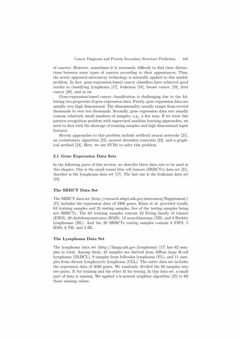
of cancers. However, sometimes it is extremely difficult to find clear distinc-tions between some types of cancers according to their appearances. Thus,the newly appeared microarray technology is naturally applied to this muddyproblem. In fact, gene-expression-based cancer classifiers have achieved goodresults in classifying lymphoma [17], leukemia [18], breast cancer [19], livercancer [20], and so on.

Gene-expression-based cancer classification is challenging due to the fol-lowing two properties of gene expression data. Firstly, gene expression data areusually very high dimensional. The dimensionality usually ranges from severalthousands to over ten thousands. Secondly, gene expression data sets usuallycontain relatively small numbers of samples, e.g., a few tens. If we treat thispattern recognition problem with supervised machine learning approaches, weneed to deal with the shortage of training samples and high dimensional inputfeatures.

Recent approaches to this problem include artificial neural networks [21],an evolutionary algorithm [22], nearest shrunken centroids [23], and a graph-ical method [24]. Here, we use SVMs to solve this problem.

2.1 Gene Expression Data Sets

In the following parts of this section, we describe three data sets to be used inthis chapter. One is the small round blue cell tumors (SRBCTs) data set [21].Another is the lymphoma data set [17]. The last one is the leukemia data set[18].

The SRBCT Data Set

The SRBCT data set (http://research.nhgri.nih.gov/microarray/Supplement/)[21] includes the expression data of 2308 genes. Khan et al. provided totally63 training samples and 25 testing samples, five of the testing samples beingnot SRBCTs. The 63 training samples contain 23 Ewing family of tumors(EWS), 20 rhabdomyosarcoma (RMS), 12 neuroblastoma (NB), and 8 Burkittlymphomas (BL). And the 20 SRBCTs testing samples contain 6 EWS, 5RMS, 6 NB, and 3 BL.

The Lymphoma Data Set

The lymphoma data set (http://llmpp.nih.gov/lymphoma) [17] has 62 sam-ples in total. Among them, 42 samples are derived from diffuse large B-celllymphoma (DLBCL), 9 samples from follicular lymphoma (FL), and 11 sam-ples from chronic lymphocytic lymphoma (CLL). The entire data set includesthe expression data of 4026 genes. We randomly divided the 62 samples intotwo parts, 31 for training and the other 31 for testing. In this data set, a smallpart of data is missing. We applied a k-nearest neighbor algorithm [25] to fillthose missing values.

346 F. Chu et al.

The Leukemia Data Set

The leukemia data set (www-genome.wi.mit.edu/MPR/data_set_ALL_AML.html) [18] contains two types of samples, i.e. the acute myeloid leukemia(AML) and the acute lymphoblastic leukemia (ALL). Golub et al. provided38 training samples and 34 testing samples. The entire leukemia data setcontains the expression data of 7129 genes.

Ordinarily, raw gene expression data should be normalized to reduce thesystemic bias introduced during experiments. For the SRBCT and the lym-phoma data sets, normalized data can be found on the web. However, for theleukemia data set, such normalized data are not available. Thereafter, we needto do normalization ourselves.

We followed the normalization procedure used in [26]. Three steps weretaken, i.e., (a) setting threshold with a floor of 100 and a ceiling of 16000, thatis, if a value is greater (smaller) than the ceiling (floor), this value is replacedby the ceiling (floor); (b) filtering, leaving out the genes with max /min ≤ 5or (max−min) ≤ 500 (max and min refer to the maximum and minimumof the expression values of a gene, respectively); (c) carrying out logarithmictransformation with 10 as the base to all the expression values. 3571 genessurvived after these three steps. Furthermore, the data were standardizedacross experiments, i.e., subtracted by the mean and divided by the standarddeviation of each experiment.

2.2 A T-Test-Based Gene Selection Approach

The t-test is a statistical method proposed by Welch [27] to measure howlarge the difference is between the distributions of two groups of samples. Ifa gene shows large distinctions between 2 groups, the gene is important forclassification of the two groups. To find the genes that contribute most toclassification, t-test has been used in gene selection [28] in recent years.

Selecting important genes using t-test involves several steps. In the firststep, a score based on the t-test (named t-score or TS) is calculated for eachgene. In the second step, all the genes are rearranged according to their TSs.The gene with the largest TS is put in the first place of the ranking list,followed by the gene with the second largest TS, and so on.

Finally, only some top genes in the list are used for classification. The stan-dard t-test is applicable to measure the difference between only two groups.Therefore, when the number of classes is more than two, we need to modifythe standard t-test. In this case, we use the t-test to measure the differencebetween one specific class and the centroid of all the classes. Hence, the defi-nition of the TS for gene i can be described as follows:


TSi = max{∣∣∣∣xik − xi

mksi

∣∣∣∣ , k = 1, 2, . . . K

}

(1)

xik =∑

j∈Ck

xij/nk (2)

xi =n∑

j=1

xij/n (3)

s2i =

1n−K

∑

k

∑

j∈Ck

(xij − xik)2 (4)

mk =√

1/nk + 1/n (5)

There are K classes. max{yk, k = 1, 2, . . . K} is the maximum of all yk. Ck

refers to class k that includes nk samples. xij is the expression value of genei in sample j. xik is the mean expression value in class k for gene i. n is thetotal number of samples. xi is the general mean expression value for gene i.si is the pooled within-class standard deviation for gene i.

2.3 Experimental Results

We applied the above gene selection approach and the C-SVC to process theSRBCT, the lymphoma, and the leukemia data sets.

Results for the SRBCT Data Set

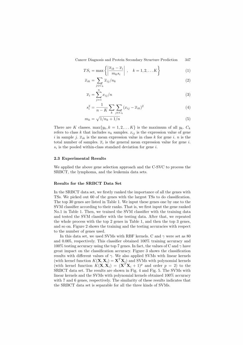
In the SRBCT data set, we firstly ranked the importance of all the genes withTSs. We picked out 60 of the genes with the largest TSs to do classification.The top 30 genes are listed in Table 1. We input these genes one by one to theSVM classifier according to their ranks. That is, we first input the gene rankedNo.1 in Table 1. Then, we trained the SVM classifier with the training dataand tested the SVM classifier with the testing data. After that, we repeatedthe whole process with the top 2 genes in Table 1, and then the top 3 genes,and so on. Figure 2 shows the training and the testing accuracies with respectto the number of genes used.

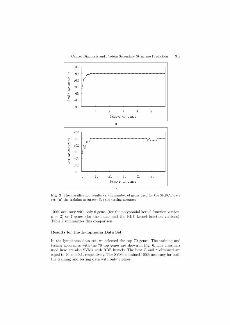
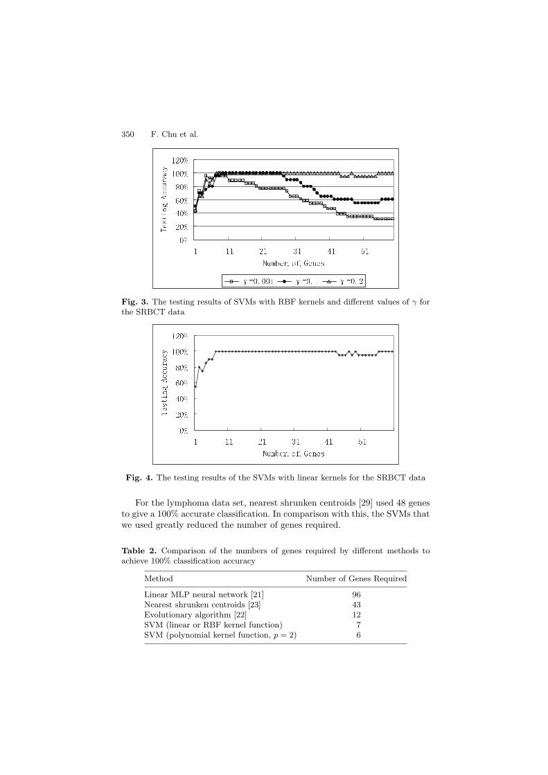
In this data set, we used SVMs with RBF kernels. C and γ were set as 80and 0.005, respectively. This classifier obtained 100% training accuracy and100% testing accuracy using the top 7 genes. In fact, the values of C and γ havegreat impact on the classification accuracy. Figure 3 shows the classificationresults with different values of γ. We also applied SVMs with linear kernels(with kernel function K(X,Xi) = XT Xi) and SVMs with polynomial kernels(with kernel function K(X,Xi) = (XT Xi + 1)p and order p = 2) to theSRBCT data set. The results are shown in Fig. 4 and Fig. 5. The SVMs withlinear kernels and the SVMs with polynomial kernels obtained 100% accuracywith 7 and 6 genes, respectively. The similarity of these results indicates thatthe SRBCT data set is separable for all the three kinds of SVMs.

348 F. Chu et al.

Table 1. The 30 top genes selected by the t-test in the SRBCT data set

Rank Gene ID Gene Description

1 810057 cold shock domain protein A2 784224 fibroblast growth factor receptor 43 296448 insulin-like growth factor 2 (somatomedin A)4 770394 Fc fragment of IgG, receptor, transporter, alpha5 207274 Human DNA for insulin-like growth factor II (IGF-2); exon 7

and additional ORF6 244618 ESTs7 234468 ESTs8 325182 cadherin 2, N-cadherin (neuronal)9 212542 Homo sapiens mRNA; cDNA DKFZp586J2118 (from clone DK-

FZp586J2118)10 377461 caveolin 1, caveolae protein, 22 kD11 41591 meningioma (disrupted in balanced translocation) 112 898073 transmembrane protein13 796258 sarcoglycan, alpha (50kD dystrophin-associated glycoprotein)14 204545 ESTs15 563673 antiquitin 116 44563 growth associated protein 4317 866702 protein tyrosine phosphatase, non-receptor type 13 (APO-

1/CD95 (Fas)-associated phosphatase)18 21652 catenin (cadherin-associated protein), alpha 1 (102 kD)19 814260 follicular lymphoma variant translocation 120 298062 troponin T2, cardiac21 629896 microtubule-associated protein 1B22 43733 glycogenin 223 504791 glutathione S-transferase A424 365826 growth arrest-specific 125 1409509 troponin T1, skeletal, slow26 1456900 Nil27 1435003 tumor necrosis factor, alpha-induced protein 628 308231 Homo sapiens incomplete cDNA for a mutated allele of a myosin

class I, myh-1c29 241412 E74-like factor 1 (ets domain transcription factor)30 1435862 antigen identified by monoclonal antibodies 12E7, F21 and O13

For the SRBCT data set, Khan et al. [21] 100% accurately classified the4 types of cancers with a linear artificial neural network by using 96 genes.Their results and our results of the linear SVMs both proved that the classesin the SRBCT data set are linearly separable. In 2002, Tibshirani et al. [23]also correctly classified the SRBCT data set with 43 genes by using a methodnamed nearest shrunken centroids. Deutsch [22] further reduced the number ofgenes required for reliable classification to 12 with an evolutionary algorithm.Compared with these previous results, the SVMs that we used can achieve


Fig. 2. The classification results vs. the number of genes used for the SRBCT dataset: (a) the training accuracy; (b) the testing accuracy

100% accuracy with only 6 genes (for the polynomial kernel function version,p = 2) or 7 genes (for the linear and the RBF kernel function versions).Table 2 summarizes this comparison.

Results for the Lymphoma Data Set

In the lymphoma data set, we selected the top 70 genes. The training andtesting accuracies with the 70 top genes are shown in Fig. 6. The classifiersused here are also SVMs with RBF kernels. The best C and γ obtained areequal to 20 and 0.1, respectively. The SVMs obtained 100% accuracy for boththe training and testing data with only 5 genes.

350 F. Chu et al.

Fig. 3. The testing results of SVMs with RBF kernels and different values of γ forthe SRBCT data

Fig. 4. The testing results of the SVMs with linear kernels for the SRBCT data

For the lymphoma data set, nearest shrunken centroids [29] used 48 genesto give a 100% accurate classification. In comparison with this, the SVMs thatwe used greatly reduced the number of genes required.

Table 2. Comparison of the numbers of genes required by different methods toachieve 100% classification accuracy

Method Number of Genes Required

Linear MLP neural network [21] 96Nearest shrunken centroids [23] 43Evolutionary algorithm [22] 12SVM (linear or RBF kernel function) 7SVM (polynomial kernel function, p = 2) 6


Fig. 5. The testing result of the SVMs with polynomial kernels (p = 2) for theSRBCT data

Fig. 6. The classification results vs. the number of genes used for the lymphomadata set: (a) the training accuracy; (b) the testing accuracy

352 F. Chu et al.

Results for the Leukemia Data Set

Alizadeh et al. [17] built a 50-gene classifier that made 1 error in the 34testing samples; and in addition, it cannot give strong prediction to another3 samples. Nearest shrunken centroids made 2 errors among the 34 testingsamples with 21 genes [23]. As shown in Fig. 7, we used the SVMs with RBFkernels with 2 errors for the testing data but with only 20 genes.

Fig. 7. The classification results vs. the number of genes used for the leukemia dataset: (a) the training accuracy; (b) the testing accuracy


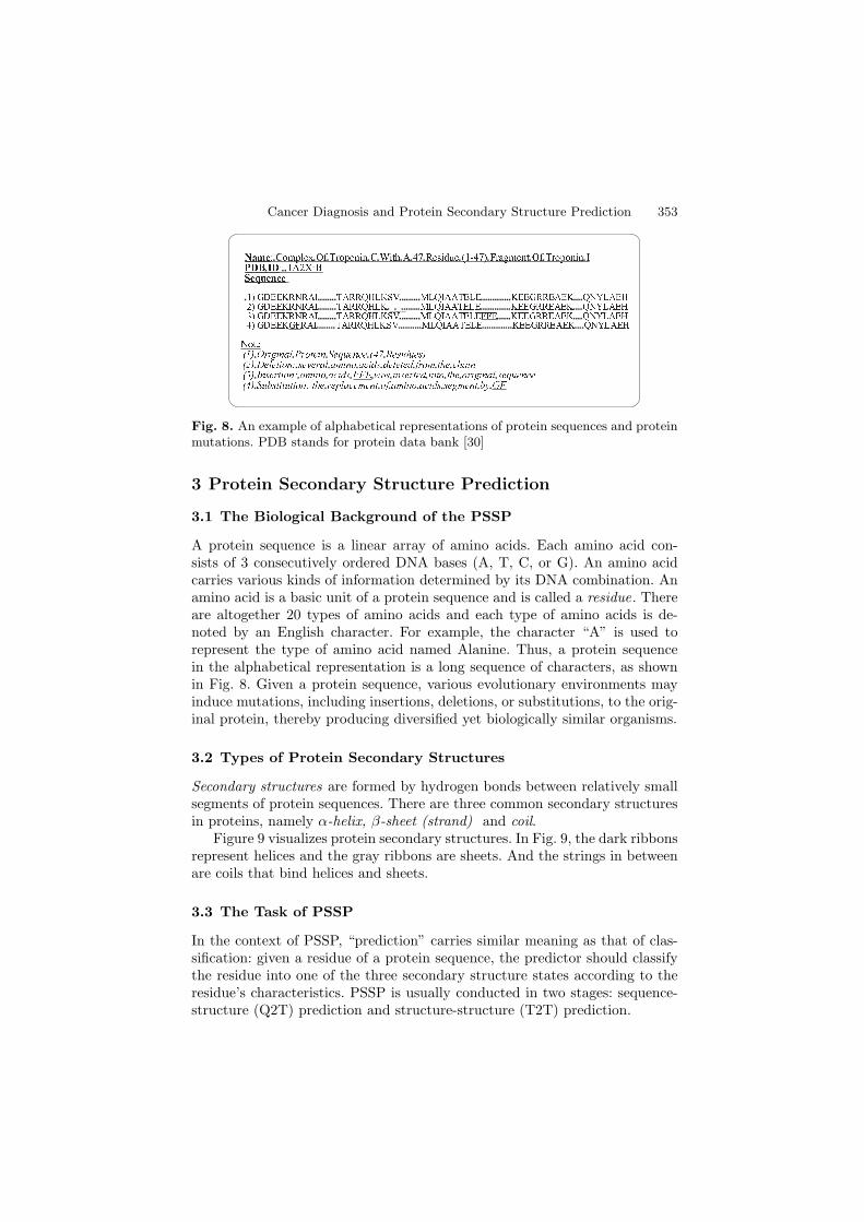
Fig. 8. An example of alphabetical representations of protein sequences and proteinmutations. PDB stands for protein data bank [30]

3 Protein Secondary Structure Prediction

3.1 The Biological Background of the PSSP

A protein sequence is a linear array of amino acids. Each amino acid con-sists of 3 consecutively ordered DNA bases (A, T, C, or G). An amino acidcarries various kinds of information determined by its DNA combination. Anamino acid is a basic unit of a protein sequence and is called a residue. Thereare altogether 20 types of amino acids and each type of amino acids is de-noted by an English character. For example, the character “A” is used torepresent the type of amino acid named Alanine. Thus, a protein sequencein the alphabetical representation is a long sequence of characters, as shownin Fig. 8. Given a protein sequence, various evolutionary environments mayinduce mutations, including insertions, deletions, or substitutions, to the orig-inal protein, thereby producing diversified yet biologically similar organisms.

3.2 Types of Protein Secondary Structures

Secondary structures are formed by hydrogen bonds between relatively smallsegments of protein sequences. There are three common secondary structuresin proteins, namely α-helix, β-sheet (strand) and coil.

Figure 9 visualizes protein secondary structures. In Fig. 9, the dark ribbonsrepresent helices and the gray ribbons are sheets. And the strings in betweenare coils that bind helices and sheets.

3.3 The Task of PSSP

In the context of PSSP, “prediction” carries similar meaning as that of clas-sification: given a residue of a protein sequence, the predictor should classifythe residue into one of the three secondary structure states according to theresidue’s characteristics. PSSP is usually conducted in two stages: sequence-structure (Q2T) prediction and structure-structure (T2T) prediction.

354 F. Chu et al.

Secondary Structure

Dark Ribbon :a -helix

Gray Ribbon :ß-sheet

String :coil

Fig. 9. Three types of protein secondary structures: α-helix, β-strand, and coil

Sequence-Structure (Q2T) Prediction

Q2T prediction predicts the protein secondary structure from protein se-quences. Given a protein sequence, a Q2T predictor maps each residue of thesequence to a relevant secondary structure state by inspecting the distinctcharacteristics of the residue, e.g., the type of the amino acid, the sequencecontext (that is, what are the neighboring residues), and evolutionary infor-mation. The sequence-structure prediction plays the most important role inPSSP.

Structure-Structure (T2T) Prediction

For common pattern classification problems, it would be the end of the taskonce each data point (each residue in our case) has been assigned a class label.Classification usually do not continue to a second phase. However, the prob-lem we are dealing with is different from most pattern recognition problems.In a typical pattern classification problem, the data points are assumed to beindependent. But this is not true for the PSSP problem because the neigh-boring sequence positions usually provide some meaningful information. Forexample, an α-helix usually consists of at least 3 consecutive residues of thesame secondary structure state (e.g., . . . ααα . . .). Therefore, if an alternativeoccurrence of the α-helix and the β-strand (e.g., . . . αβαβ . . .) is predicted, itwould be incorrect. Thus, T2T prediction based on the Q2T results is usuallycarried out. This step helps to correct errors incurred in Q2T prediction andhence enhances the overall prediction accuracy. Figure 10 illustrates PSSPwith the two stages.

Note that amino acids of the same type do not always have the same sec-ondary structure state. For instance, in Fig. 10, the 12 -th and the20 -th amino residues counted from the left side are both F. However, theyare assigned to two different secondary structure states, i.e., α and β.


Fig. 10. Protein secondary structure prediction: the two-stage approach

Prediction of the secondary structure state at each sequence positionshould not solely rely on the residue at that position. A window expandingtowards both directions of the residue should be used to include the sequencecontext.

3.4 Methods for PSSP

PSSP was stimulated by research on protein 3D structures in the 1960s [31,32], which attempted to find the correlations between protein sequences andsecondary structures. This was the first generation of PSSP, where most meth-ods carried out prediction based on single residue statistics [33, 34, 35, 36, 37].Since only particular types of amino acids from protein sequences were ex-tracted and used in experiments, the accuracies of these methods were moreor less over-estimated [38].

With growth of knowledge on protein structures, the second generationPSSP made use of segment statistics. A segment of residues was studied tofind out how likely the central residue of the segment belonged to a secondarystructure state. Algorithms of this generation include statistical information[36, 40], sequence patterns [41, 42], multi-layer networks [43, 44, 45, 49], mul-tivariate statistics [46], nearest-neighbor algorithms [47], etc.

Unfortunately, the methods in both the first and the second generationscould not reach an accuracy higher than 70%.

The earliest application of artificial neural networks to PSSP was carriedout by Qian and Sejnowski in 1988 [48]. They used a three-layered back-propagation network whose input data was encoded with a scheme calledBIN21. Under BIN21, each input data was a sliding window of 13 residuesobtained by extending 6 sequence positions from the central residue. The fo-cus of each observation was only on the central residue, i.e., only the centralresidue was assigned to one of the three possible secondary structure states

356 F. Chu et al.

(α-helix, β-strand, and coil). Modifications to the BIN21 scheme were intro-duced in two later studies. Kneller et al. [49] added one additional input unitto present the hydrophobicity scale of each amino acid residue and showed aslightly higher accuracy. Sasagawa and Tajima [51] used the BIN24 scheme toencode three additional amino acid alphabets, B, X, and Z. The above earlywork had an accuracy ceiling of 65%. In 1995, Vivarelli et al. [52] used a hybridsystem that combined a Local Genetic Algorithm (LGA) and neural networksfor PSSP. Although LGA was able to select network topologies efficiently, itstill could not break through the accuracy ceiling, regardless of the networkarchitectures applied.

A significant improvement of the 3-state secondary structure predictioncame from Rost and Sander’s method (PHD) [53, 54], which was based ona multi-layer back-propagation network. Different from the BIN21 codingscheme, PHD took into account evolutionary information in the form of mul-tiple sequence alignments to represent the input data. This inclusion of theprotein family information improved the prediction accuracy by around sixpercentages. Moreover, another cascaded neural network conducted structure-structure prediction. Using the 126 protein sequences (RS126) developed bythemselves, Rost and Sander achieved the overall accuracy as high as 72%.

In 1999, Jones [56] used a Position-Specific Scoring Matrix (PSSM) [57, 58]obtained from the online alignment searching tool PSI-Blast (http://www.ncbi.nlm.nih.gov/BLAST/) to numerically represent the protein sequence. APSSM was constructed automatically from a multiple alignment of the high-est scoring hits in an initial BLAST search. The PSSM was generated bycalculating position-specific scores for each position in the alignment. Highlyconserved positions of protein sequence received high scores and weakly con-served positions received scores near zero. Due to its high accuracy in findingthe biologically similar protein sequences, the evolutionary information carriedby the PSSM is more sensitive than the profiles obtained by other multiplesequence alignment approaches. With a neural network similar to that of Rostand Sander’s, Jones’ PSIPRED method achieved an accuracy as high as 76.5%using a much larger data set than RS126.

In 2001, Hua and Sun [6] proposed an SVM approach. This was an earlyapplication of the SVM to the PSSP problem. In their work, they first con-structed 3 one-versus-one and 3 one-versus-all binary classifiers. Three tertiaryclassifiers were designed based on these binary classifiers through the use ofthe largest response, the decision tree and votes for the final decision. Bymaking use of the Rost’s data encoding scheme, they achieved the accuracyof 71.6% and the segment overlap accuracy of 74.6% for the RS126 data set.

4 SVMs for the PSSP Problem

In this section, we use the LIBSVM, or more specially, the C-SVC, to solvethe PSSP problem.


The data set used here was originally developed and used by Jones [56].This data set can be obtained from the website (http://bioinf.cs.ucl.ac.uk/psipred/). The data set contains a total of 2235 protein sequences for trainingand 187 sequences for testing. All the sequences in this data set have beenprocessed by the online alignment searching tool PSI-Blast (http://www.ncbi.nlm.nih.gov/BLAST/).

As mentioned above, we will conduct PSSP in two stages, i.e., Q2T pre-diction and T2T prediction.

4.1 Q2T Prediction

Parameter Tuning Strategy

For PSSP, there are three parameters, i.e., the window size N , and SVMparameters (C,γ), to be tuned. N determines the span of the sliding window,i.e., how many neighbors to be included in the window. Here, we test fourdifferent values for N , i.e., 11, 13, 15, and 17.

Searching for the optimal (C, γ) pair is also difficult because the dataset used here is extremely large. In [50], Lin and Lin found an optimal pair,(C, γ) = (2, 0.125), for the PSSP problem with a much smaller data set (about10 times smaller compared to the data set used here). Despite the difference ofdata sizes, we find that their optimal pair also benefits our search as a properstarting point. During our search, we change only one parameter at a time.If the change (increase/decrease) leads to a higher accuracy, we continue todo a similar change (increase/decrease) next time; otherwise, we reverse thechange (decrease/increase). Both C and γ are tuned with this scheme.

Results

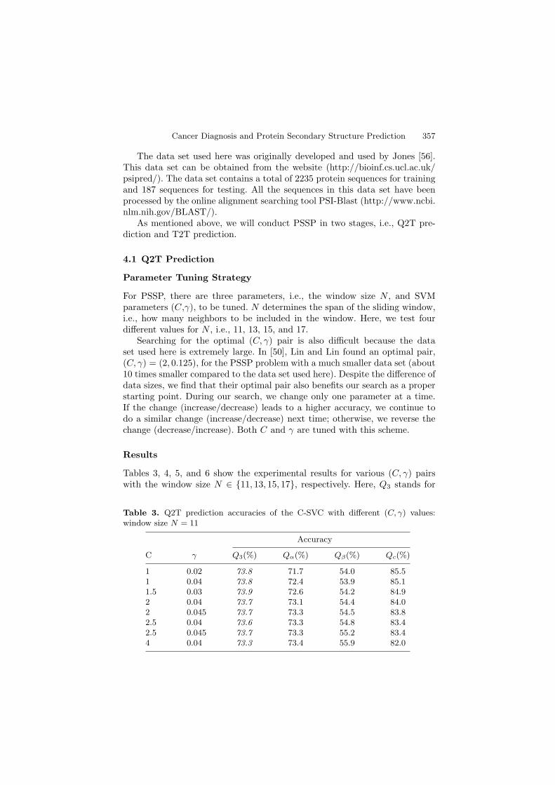
Tables 3, 4, 5, and 6 show the experimental results for various (C, γ) pairswith the window size N ∈ {11, 13, 15, 17}, respectively. Here, Q3 stands for

Table 3. Q2T prediction accuracies of the C-SVC with different (C, γ) values:window size N = 11

Accuracy

C γ Q3(%) Qα(%) Qβ(%) Qc(%)

1 0.02 73.8 71.7 54.0 85.51 0.04 73.8 72.4 53.9 85.11.5 0.03 73.9 72.6 54.2 84.92 0.04 73.7 73.1 54.4 84.02 0.045 73.7 73.3 54.5 83.82.5 0.04 73.6 73.3 54.8 83.42.5 0.045 73.7 73.3 55.2 83.44 0.04 73.3 73.4 55.9 82.0

358 F. Chu et al.


Accuracy

C γ Q3(%) Qα(%) Qβ(%) Qc(%)

1 0.02 73.9 72.3 54.8 84.91.5 0.008 73.6 71.4 54.3 85.01.5 0.02 73.9 72.6 54.7 84.81.7 0.04 74.1 73.6 54.8 83.42 0.025 74.0 73.0 55.1 84.32 0.04 74.1 73.9 55.0 83.92 0.045 74.2 74.1 55.9 83.54 0.04 73.2 73.9 55.5 81.7


Accuracy

C γ Q3(%) Qα(%) Qβ(%) Qc(%)

2 0.006 73.4 70.8 54.2 85.22 0.03 74.1 73.6 55.6 84.02 0.04 74.2 73.9 55.7 83.72 0.045 74.0 73.7 55.4 83.72 0.05 74.0 73.7 55.4 83.62 0.15 69.0 63.3 32.7 91.92.5 0.02 74.0 73.0 55.6 84.02.5 0.03 74.1 74.0 55.9 83.54 0.025 74.0 73.8 55.8 83.4


Accuracy

C γ Q3(%) Qα(%) Qβ(%) Qc(%)

1 0.125 70.0 63.6 36.0 91.32 0.03 74.1 73.5 56.2 83.72.5 0.001 71.3 68.1 52.4 83.52.5 0.02 74.0 68.1 52.4 83.52.5 0.04 74.0 75.0 55.8 83.1

the overall accuracy; Qα, Qβ , and Qc are the accuracies for α-helix, β-strand,and coil, respectively.

From these tables, we could see that the optimal (C, γ) values for win-dow size N ∈ {11, 13, 15, 17} are (1.5, 0.03), (2, 0.045), (2, 0.04), and (2, 0.03),


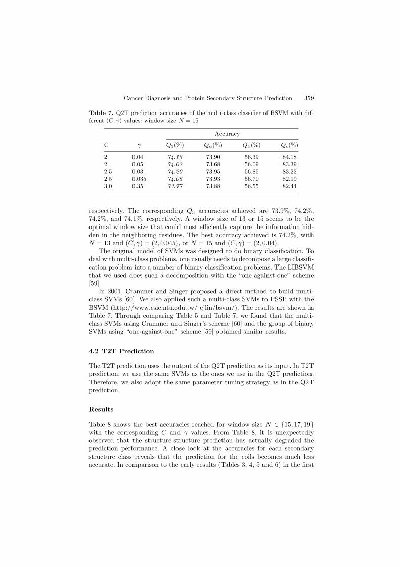
Table 7. Q2T prediction accuracies of the multi-class classifier of BSVM with dif-ferent (C, γ) values: window size N = 15

Accuracy

C γ Q3(%) Qα(%) Qβ(%) Qc(%)

2 0.04 74.18 73.90 56.39 84.182 0.05 74.02 73.68 56.09 83.392.5 0.03 74.20 73.95 56.85 83.222.5 0.035 74.06 73.93 56.70 82.993.0 0.35 73.77 73.88 56.55 82.44

respectively. The corresponding Q3 accuracies achieved are 73.9%, 74.2%,74.2%, and 74.1%, respectively. A window size of 13 or 15 seems to be theoptimal window size that could most efficiently capture the information hid-den in the neighboring residues. The best accuracy achieved is 74.2%, withN = 13 and (C, γ) = (2, 0.045), or N = 15 and (C, γ) = (2, 0.04).

The original model of SVMs was designed to do binary classification. Todeal with multi-class problems, one usually needs to decompose a large classifi-cation problem into a number of binary classification problems. The LIBSVMthat we used does such a decomposition with the “one-against-one” scheme[59].

In 2001, Crammer and Singer proposed a direct method to build multi-class SVMs [60]. We also applied such a multi-class SVMs to PSSP with theBSVM (http://www.csie.ntu.edu.tw/ cjlin/bsvm/). The results are shown inTable 7. Through comparing Table 5 and Table 7, we found that the multi-class SVMs using Crammer and Singer’s scheme [60] and the group of binarySVMs using “one-against-one” scheme [59] obtained similar results.

4.2 T2T Prediction

The T2T prediction uses the output of the Q2T prediction as its input. In T2Tprediction, we use the same SVMs as the ones we use in the Q2T prediction.Therefore, we also adopt the same parameter tuning strategy as in the Q2Tprediction.

Results

Table 8 shows the best accuracies reached for window size N ∈ {15, 17, 19}with the corresponding C and γ values. From Table 8, it is unexpectedlyobserved that the structure-structure prediction has actually degraded theprediction performance. A close look at the accuracies for each secondarystructure class reveals that the prediction for the coils becomes much lessaccurate. In comparison to the early results (Tables 3, 4, 5 and 6) in the first

360 F. Chu et al.

Table 8. The T2T prediction accuracies for window size N = 15, 17, and 19

AccuracyWindowSize (N) C γ Q3(%) Qα(%) Qβ(%) Qc(%)

15 1 2−5 72.6 77.9 60.8 74.317 1 2−4 72.6 78.0 60.4 74.519 1 2−6 72.8 78.2 60.1 74.9

stage, the Qc accuracy dropped from 84% to 75%. By sacrificing the accuracyfor coils, the predictions for the other two secondary structures improved.However, because coils have a much larger population than the other twokinds of secondary structures, the overall 3-state accuracy Q3 decreased.

5 Conclusions

To sum up, SVMs performs well in both bioinformatics problems that wediscussed in this chapter. For the problem of cancer diagnosis based on mi-croarray data, the SVMs that we used outperformed most of the previouslyproposed methods in terms of the number of genes required and the accu-racy. Therefore, we conclude that the SVMs can not only make highly reliableprediction, but also can reduce redundant genes. For the PSSP problem, theSVMs also obtained results comparable with those obtained by other ap-proaches.

References

1. Cortes C, Vapnik VN (1995) Support vector networks. Machine Learning20:273–297

2. Vapnik VN (1995) The nature of statistical learning theory. Springer-Verlag,New York

3. Vapnik VN (1998) Statistical learning theory. Wiley, New York4. Drucker N, Donghui W, Vapnik VN (1999) Support vector machines for spam

categorization. IEEE Transaction on Neural Networks 10:1048–10545. Chapelle O, Haffner P, Vapnik VN (1999) Support vector machines for

histogram-based image classification. IEEE Transaction on Neural Networks10:1055–1064

6. Hua S, Sun Z (2001) A novel method of protein secondary structure predictionwith high segment overlap measure: support vector machine approach. Journalof molecular Biology 308:397–407

7. Strauss DJ, Steidl G (2002) Hybrid wavelet-support vector classification of wave-forms. J Comput and Appl 148:375–400

8. Kumar R, Kulkarni A, Jayaraman VK, Kulkarni BD (2004) Symbolization as-sisted SVM classifier for noisy data. Pattern Recognition Letters 25:495–504


9. Mukkamala S, Sung AH, Abraham A (2004) Intrusion detection using an ensem-ble of intelligent paradigms. Journal of Network and Computer Applications, InPress

10. Norinder U (2003) Support vector machine models in drug design: applicationsto drug transport processes and QSAR using simplex optimisations and variableselection. Neurocomputing 55:337–346

11. Van GT, Suykens JAK, Baestaens DE, Lambrechts A, Lanckriet G, VandaeleB, De Moor B, Vandewalle J (2001) Financial time series prediction using leastsquares support vector machines within the evidence framework. IEEE Trans-actions on Neural Networks 12:809–821

12. Chang CC, Lin CJ LIBSVM: A library for support vector machines. availableat http://www.csie.ntu.edu.tw/˜cjlin/libsvm

13. Scholkopf B, Smolar A, Williamson RC, Bartlett PL (2000) New support vectoralgorithms. Neural Computation 12:1207–1245

14. Schoklopf B, Platt JC, Shawe-Taylor J, Smola AJ, Williamson RC (2001) Es-timating the support of a high-dimensional distribution. Neural Computation13:443–1471

15. Slonim DK (2002) From patterns to pathways: gene expression data analysiscomes of age. Nature Genetics Suppl. 32:502–508

16. Russo G, Zegar C, Giordano A (2003) Advantages and limitations of microarraytechnology in human cancer. Oncogene 22:6497–6507

17. Alizadeh AA, Eisen MB, Davis RE, Ma C, Lossos IS, Rosenwald A, BoldrickJC, Sabet H, Tran T, Yu X, et al. (2000) Distinct types of diffuse large B-celllymphoma identified by gene expression profiling. Nature 403:503–511

18. Golub TR, Slonim DK, Tamayo P, Huard C, Gaasenbeek M, Mesirov JP, CollerH, Loh ML, Downing JR, Caligiuri MA et al. (1999) Molecular classificationof cancer: class discovery and class prediction by gene expression monitoring.Science 286:531–537

19. Ma X, Salunga R, Tuggle JT, Gaudet J, Enright E, McQuary P, Payette T,Pistone M, Stecker K, Zhang BM et al. (2003) Gene expression profiles of humanbreast cancer progression. Proc Natl Acad Sci USA 100:5974–5979

20. Chen X, Cheung ST, So S, Fan ST, Barry C (2002) Gene expression patternsin human liver cancers. Molecular Biology of Cell 13:1929–1939

21. Khan J, Wei JS, Ringner M, Saal LH, Ladanyi M et al. (2001) Classificationand diagnostic prediction of cancers using gene expression profiling and artificialneural networks. Nature Medicine 7:673–679

22. Deutsch JM (2003) Evolutionary algorithms for finding optimal gene sets inmicroarray prediction. Bioinformatics 19:45–52

23. Tibshirani R, Hastie T, Narashiman B, Chu G (2002) Diagnosis of multiplecancer types by shrunken centroids of gene expression. Proc Natl Acad Sci USA99:6567–6572

24. Bura E, Pfeiffer RM (2003) Graphical methods for class prediction using dimen-sion reduction techniques on DNA microarray data. Bioinformatics 19:1252–1258

25. Troyanskaya O, Cantor M, Sherlock, G et al. (2001) Missing value estimationmethods for DNA microarrays. Bioinformatics 17:520–525

26. Dudoit S, Fridlyand J, Speed T (2002) Comparison of discrimination methodsfor the classification of tumors using gene expression data. J Am Stat Assoc97:77–87

362 F. Chu et al.

27. Welch BL (1947) The generalization of student’s problem when several differentpopulation are involved. Biomethika 34:28–35

28. Tusher, VG, Tibshirani R, Chu G (2001) Significance analysis of microarraysapplied to the ionizing radiation response. Proc Natl Acad Sci USA 98:5116–5121

29. Tibshirani R, Hastie T, Narasimhan B, Chu G (2003) Class prediction by nearestshrunken centroids with applications to DNA microarrays. Statistical Science18:104–117

30. Berman HM, Westbrook J, Feng Z, Gilliland G, Bhat TN, Weissig H, ShindyalovIN, Bourne PE (2000) The protein data bank. Nucleic Acids Research 28:235–242

31. Kendrew JC, Dickerson RE, Strandberg BE, Hart RJ, Davies DR et al. (1960)Structure of myoglobin: a three-dimensional fourier synthesis at 2 A resolution.Nature 185:422–427

32. Perutz MF, Rossmann MG, Cullis AF, Muirhead G, Will G et al. (1960) Struc-ture of haemoglobin: a three-dimensional fourier synthesis at 5.5 A resolution.Nature 185:416–422

33. Scheraga HA (1960) Structural studies of ribonuclease III. A model for thesecondary and tertiary struture. J Am Chem Soc 82:3847–3852

34. Davids DR (1964) A correlation between amino acid composition and proteinstructure. Journal of Molecular Biology 9:605–609

35. Robson B, Pain RH (1971) Analysis of the code relating sequence to conforma-tion in proteins: possible implications for the mechanism of formation of helicalregions. Journal of Molecular Biology 58:237–259

36. Chou PY, Fasma UD (1974) Prediction of protein conformation. Biochem13:211–215

37. Lim VI (1974) Structural principles of the globular organization of proteinchains. A stereochemical theory of globular protein secondary structure. Journalof Molecular Biology 88:857–872

38. Rost B, Sander C (1994) Combining evolutionary information and neural net-works to predict protein secondary structure. Proteins 19:55–72

39. Robson B (1976) Conformational properties of amino acid residues in globularproteins. Journal of Molecular Biology 107:327–56

40. Nagano K (1977) Triplet information in helix prediction applied to the analysisof super-secondary structures. Journal of Molecular Biology 109:251–274

41. Taylor WR, Thornton JM (1983) Prediction of super-secondary structure inproteins. Nature 301:540–542

42. Rooman MJ, Kocher JP, Wodak SJ (1991) Prediction of protein backbone con-formation based on seven structure assignments: influence of local interactions.Journal of Molecular Biology 221:961–979

43. Bohr H, Bohr J, Brunak S, Cotterill RMJ, Lautrup B et al (1988) Proteinsecondary structure and homology by neural networks. FEBS Lett 241:223–228

44. Holley HL, Karplus M (1989) Protein secondary structure prediction with aneural network. Proc Natl Acad Sci USA 86:152–156

45. Stolorz P, Lapedes A, Xia Y (1992) Predicting protein secondary structure usingneural net and statistical methods. Journal of Molecular Biology 225:363–377

46. Muggleton S, King RD, Sternberg MJE (1992) Protein secondary structure pre-dictions using logic-based machine learning. Prot Engin 5:647–657


47. Salamov AA, Solovyev VV (1995) Prediction of protein secondary structure bycombining nearest-neighbor algorithms and multiple sequence alignment. Jour-nal of Molecular Biology 247:11–15

48. Qian N, Sejnowski TJ (1988) Predicting the secondary structure of globularproteins using neural network models. Journal of Molecular Biology 202:865–84

49. Kneller DG, Cohen FE, Langridge R (1990) Improvements in protein secondarystructure prediction by an enhanced neural network. Journal of Molecular Biol-ogy 214:171–82

50. Lin KM, Lin CJ (2003) A study on reduced support vector machines. IEEETransactions on Neural Networks 12:1449–1559

51. Sasagawa F, Tajima K (1993) Prediction of protein secondary structures by aneural network. Computer Applications in the Biosciences 9:147–152

52. Vivarelli F, Giusti G, Villani M, Campanini R, Fraiselli P, Compiani M, CasadioR (1995) LGANN: a parallel system combining a local genetic algorithm andneural networks for the prediction of secondary structure of proteins. ComputerApplication in the Biosciences 11:763–9

53. Rost B, Sander C (1993) Prediction of protein secondary structure at betterthan 70% accuracy. Journal of Molecular Biology 232:584–599

54. Rost B (1996) PHD: predicting one-dimensional protein secondary structure byprofile-based neural network. Methods in Enzymology 266:525–539

55. Riis SK, Krogh A (1995) Improving prediction of protein secondary structureusing structured neural networks and multiple sequence alignments. Journal ofComputational Biology 3:163–183

56. Jones DT (1999) Protein secondary structure prediction based on position-specific scoring matrices. Journal of Molecular Biology 292:195–202

57. Stephen FA, Warren G, Webb M, Engene WM, David JL (1990) Basic localalignment search tool. Journal of Molecular Biology 215:403–410

58. Altschul SF, Schaffer AA, Zhang J, Zhang Z, Miller W, Lipman FJ (1997)Gapped BLAST and PSI-BLAST: a new generation of protein database searchprograms. Nucleic Acids Research 25:3389–3402

59. Hsu CW, Lin CJ (2002) A comparison of methods for multiclass support vectormachines. IEEE Transactions on Neural Networks 13:415–425

60. Crammer K, Singer Y (2001) On the algorithmic implementation of multiclasskernel-based vector machines. Journal of Machine Learning Research 2:265–292

support vector machines: theory and applications · preface the support vector machine (svm) is a...

Documents