support for water sector plan development

Support for water sector plan

development – Garissa County Assessment of the water availability and demand

Kenya RAPID Program

Oct 12, 2017

Draft report

ii

Draft report

Colophon

Document title . Support for water sector plan development

Client . Millennium Water Alliance

Status . Draft report

Datum . Oct 12, 2017

Project number . 611

Author(s) . S. Burger, D. Benedicto van Dalen, S. de Wildt,

R.C. van der Meulen

Executive summary

This report is established to support informed decision making and strategies for

sustainable development and use of water sources and infrastructure for multiple users

in Garissa County. It is based on the principles of Integrated Water Resources

Management (IWRM), taking into account all main elements determining the water

availability in the current situation and in the future. It will support decisions on which

kind of resource (e.g. groundwater abstraction or rainwater harvesting) can best be

developed for which kind of specific use in time and space.

The water demand analysis for Garissa County shows that the total water demand is very

small (less than 1%) compared to the three months with rainwater surplus in an average

rainfall year (April, May and November). To meet the water demand necessities, decision

makers need to face the challenge of planning and developing infrastructure based on

the principles of IWRM. The different demands need to be met not only in terms of

quantity and quality, but also in terms of time and space. Rainwater harvesting is

therefore the most sustainable way, since it is the largest water input and recharged

every year. Other opportunities can be found in the use of river discharge and the

groundwater resources. Both need to be evaluated carefully to be developed in a

sustainable way to avoid overexploitation and generate conflict among the different

users group.

The biophysical landscape of Garissa County also provides very effective, low-cost

alternatives for the harvesting and buffering of (rain) water through 3R measures,

especially for times of high needs (droughts). In Garissa County storage of rainwater

mainly on the ground, and in some parts also in the ground shows a lot of potential for

interventions such as road water harvesting, water pans and sand dams.

Support for water sector plan development - iii -

Table of contents

1 Introduction ..................................................................................................................... 1

2 Biophysical landscape................................................................................................... 2

Topography .................................................................................................................................... 2

Soils .................................................................................................................................................. 4

Land use .......................................................................................................................................... 6

Vegetation Index ........................................................................................................................... 6

Nature reserves ............................................................................................................................. 9

Geology ............................................................................................................................................ 9

3 Water availability .......................................................................................................... 11

Introduction ................................................................................................................................ 11

Precipitation ................................................................................................................................ 11

Evapotranspiration .................................................................................................................... 13

Net precipitation ........................................................................................................................ 14

River in & outflow ...................................................................................................................... 16

Groundwater resources ........................................................................................................... 18

Water quality ............................................................................................................................... 21

Water budget ............................................................................................................................... 23

4 Demand for multiple uses ............................................................................................ 24

Introduction ................................................................................................................................ 24

Domestic water demand .......................................................................................................... 24

Livestock drinking water demand ........................................................................................ 25

Rangeland water demand ........................................................................................................ 26

Agricultural water demand ..................................................................................................... 26

Wildlife drinking water ............................................................................................................ 27

Industrial water demand ......................................................................................................... 27

Conclusions on demand .......................................................................................................... 28

5 Integrating water availability and demand .............................................................. 30

Introduction ................................................................................................................................ 30

County scale balances .............................................................................................................. 30

Requirements, opportunities and challenges for meeting the water needs ............. 31

Linking water resources to demand ..................................................................................... 34

iv

Draft report

3R potential (landscape approach) ....................................................................................... 36

Deep groundwater potential .................................................................................................. 38

Grazing area potential map .................................................................................................... 40

6 Conclusions and recommendations .......................................................................... 44

Water demand and availability .............................................................................................. 44

Development of water use ...................................................................................................... 44

Water potential ........................................................................................................................... 46

Stakeholder engagement and policy integration .............................................................. 47

7 Literature ........................................................................................................................ 48

Annex 1: Calculation Water Need Tool ............................................................................. 50

Annex 2: 3R potential map .................................................................................................. 55

Annex 3: Background information BGS groundwater potential maps........................... 57

Annex 4: Sustainable agriculture in arid land ................................................................... 59

Support for water sector plan development - 1 -

1 Introduction

The goal of the Acacia Water part of the Kenya RAPID program is to support informed

decision making for policy development, and to support strategies for responsible

development and use of water sources for multiple uses. Our vision is that it will be an

integral approach, taking into account all main elements of the water demand now and

in the future and all main resources of water, so that well informed decisions for a

sustainable water supply can be made. For this an assessment framework is required to

support decisions on which kind of resource (e.g. groundwater abstraction, or rainwater

harvesting) can best be developed for which kind of use. An order of magnitude

methodology, rather than a detailed study of one of the elements, provides insight in the

full range of available resources and the natural capacity for development in the region.

Approach

The role of Acacia Water in the Kenya RAPID program is the expert partner on

biophysical and hydrogeological data requirements and information collection. Acacia

Water will assist counties to interpret the data into knowledge to support informed

decision making for policy development, and to responsibly develop and utilize existing

water sources for multiple uses through locally appropriate technologies. Existing data

available will be combined to support improved decision-making on integrated water

management of the counties.

The methodology presented in this report provides insight in the balance between the

multiple demands and supplies, the potential and the difficulties to fulfil the demand

with existing resources, the feasible infrastructure, and the potential for growth based

on the availability of the natural resources.

In line with the current livelihoods, we focus on the domestic and livestock demand and

provide additionally an indication of the possibilities for agricultural development.

Water requests from other sectors (such as industrial water demand and mining) are

mostly not available, and should be estimated based on the known data in Garissa

County.

How to read this report

Chapter 2 presents all data collected and analysed which is the base for understanding

the hydrology and hydrogeology of Garissa County in order to analyse the potential for

3R interventions. Chapter 3 presents an overview of the water resources availability,

from precipitation to surface water, from shallow to deep groundwater. In chapter 4 we

make an assessment of the demand, current and future for the different uses: domestic,

agriculture, livestock and wild life. In chapters 5 and 6 an analyses is carried out on the

opportunities and challenges to increase water availability through the potential for 3R

interventions and conclusion and recommendations are given.

- 2 - Draft report

2 Biophysical landscape

Topography

General

Garissa County borders Wajir County to the North, Isiolo County to the West, Ethiopia in

the East, and Tana River, and Lamu Counties to the South. The county covers an area of

approximately 44,459 km².

Altitude variation

Garissa County is located at the coastal plains of Kenya. Altitude variations in the

county are limited, ranging from sea level in the south eastern coastal strip to nearly

500 m a.s.l. in the north west of the county.

Figure 1: Altitude variation in the north of Kenya (based on 90m DEM – SRTM)

Slopes

The slope is an important factor for intervention suitability studies as it influences the

potential of runoff. Moreover, slope is one of the major factors determining the

potential for in-stream riverbed storage methods, as well as determining erosion control

measures.


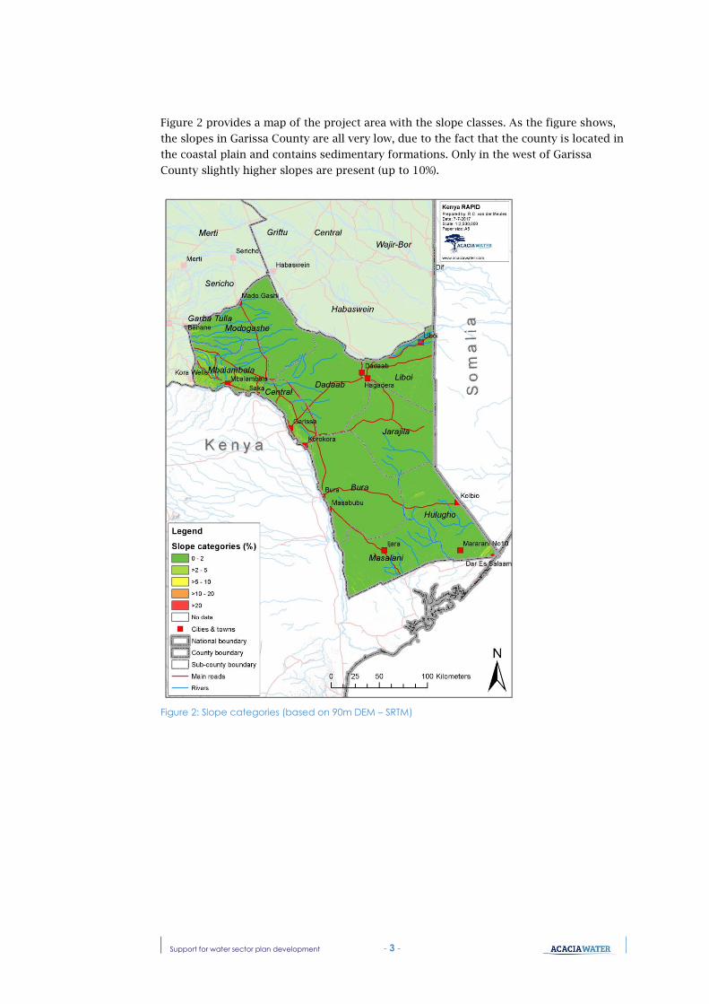
Figure 2 provides a map of the project area with the slope classes. As the figure shows,

the slopes in Garissa County are all very low, due to the fact that the county is located in

the coastal plain and contains sedimentary formations. Only in the west of Garissa

County slightly higher slopes are present (up to 10%).

Figure 2: Slope categories (based on 90m DEM – SRTM)

- 4 - Draft report

Soils

Both intervention suitability and groundwater potential are very dependent on soil -

many interventions use infiltration of surface runoff as a method of winning water,

while groundwater recharge is also directly dependent on infiltration capacity.

Infiltration capacity is very dependent on soil type. Moreover, some soils are associated

with high salinity of groundwater. Suitability for agriculture and sensitivity to land

degradation is related to soil type as well, both dependent on soil structure and texture.

Box 1 explains how soil degradation and salinization happens.

Box 1: Irrigated agriculture in arid lands: salinization will eventually

happen

All soils contain and different water sources contain a certain amount of dissolved

minerals (e.g. salts). The concentration of these minerals can change due to

evaporation of water (rise in concentration) or rainfall (lowering of the concentration).

In case of irrigated agriculture, the constant shortage of water for the plants is solved

by adding additional water from boreholes, reservoirs or rivers. This is brought to the

fields via irrigation channels and brought to the plants via flush irrigation, sprinklers

or drip irrigation.

All surplus water is lost to the ground, and will eventually evaporate into the sky.

This upward flow of water transports minerals to the surface, where only the water

evaporates and the minerals remain in the soil. The longer this upward flow occurs,

the more the salt concentration will rise.

When the concentrations of salt reach levels of 0,5 to 1,0 % the concentration becomes

toxic for most plants. When these levels are reached, soils become unfertile and can no

longer be used for cultivation. When soils have become salinized, it is very difficult

(and sometimes impossible) to reverse: it has to be flushed out to drainage channels or

to deeper layers (if groundwater levels are deep). This process however can also cause

contamination of the shallow groundwater.

In order to prevent salinization of lands, dryland farming offers good opportunities.

Worldwide more and more experience is gained in making dryland farming a profitable

business, while at the same time salinization of soils is prevented and even reduced

(due to healthy soil life).

A soil map of the project area is shown in Figure 3. Due to the constant larger

evapotranspiration than the precipitation in arid lands, soils can become saline. In the

ASAL’s in the North of Kenya contain quite some saline soils can be found (Agro-

Climatic Zones V – VII; Sombroek et al, 1982), mainly at Vertisols, Fluvisols, Solonchacks,

Solonetz, Gleysoils, Regosols, Planosols and Luvisols (Gijsbertsen, 2007).

Garissa County contains large areas with solonetz (SN), soils that can be very saline. For

these areas it is important to take soil salinity into consideration when evaluating 3R

and groundwater potential. However, a saline soil does not automatically mean that the

runoff will be saline as well. This is something that has to be evaluated during

catchment or micro-catchment assessments and when planning possible interventions.

The other main soils in Garissa County are


- Planosols (PL) - poor properties, waterlogging can occur, the soils are chemically

degraded and the surface can have become acid

- Lixisols (LX) – strongly weathered soils, which clay has washed-out down to an

subsurface horizon that has low activity clays and a high base saturation level.

- Arenosols (AR) – soils developed in residual sands with at least 35% rock or

coarse fragments

The minor spread out soils in Garissa County are:

- Gleysols (GL) - soils that are often saturated for a long time

- Vertisols (VR) - clay rich soils that develop wide cracks when drying. These soils

can be relatively saline.

- Cambisols (CM) – Soils without a layer of accumulated clay, humus, soluble salts

or iron, generally well drained.

If the soil map is compared with the slope and geology map, it can be seen that

the Cambisols are on top and downhill of the Gneisses, migmatides, quartzites

and granitoids formations

Figure 3: Soil map of Garissa County (adapted from: Sombroek et al, 1982)

- 6 - Draft report

Land use

As can be seen from Figure 4 the land use in Garissa County is mainly characterized by

rangelands (light yellow), which are being used by pastoralist communities and flood

plains. The white indicated areas are predominantly barren plains and bare rock

mountain ranges. In the South of Garissa County, between Masalani and Hulugho there

are some arable lands.

Figure 4: Interpreted land use map of Garissa County

Vegetation Index

The Normalized Difference Vegetation Index (NDVI) is a remote sensing based indicator

of greenness of an area. Tiles are available for every month. NDVI data is available since

2000. Spatial resolution of the NDVI tiles is 250 m. This NDVI is closely related to

vegetation cover and soil moisture. Values range from zero to one, representing bare

areas with no vegetation (0) to areas fully covered with vegetation (1).

All the NDVI tiles for Garissa County have been analysed. For every pixel over this whole

period of 15 year statistics have been calculated. Two images with some results of this


analysis are shown in Figure 5. On the left is the average NDVI shown for Garissa County

over the period 2000 till 2015. On the right is the variance of the NDVI in Garissa County

shown; the variance is the square of the standard deviation. This NDVI variance is a

statistical parameter that shows how strong each NDVI pixel varies in time. For example,

when the NDVI variance value is low, it means that there is limited fluctuation in the

vegetation cover. If the average NDVI is high and the variance is low, this area is always

green, while if the average NDVI is high and the variance is high, it means that some

parts of the year it is very green, while other parts of the year it is poorly vegetated.

The higher the average NDVI, the greener the colour in Figure 5 left; the lower the NDVI,

the more red. The higher the variance of the NDVI, the greener; the lower the variance of

the NDVI, the more red (Figure 5 right).

The general vegetation pattern in Garissa County is: the further from the coast, so the

dryer Garissa County becomes. This results in a NDVI that is reducing towards the North

West. Most parts not only have a low NDVI, the variance is also low, which means that it

remains poorly vegetated for most of the year. Some riverbeds have a relatively low

mean NDVI but with a NDVI variance that is a bit higher, which means that some parts

of the year, water is available for vegetation. In the south-southeast of the county

average NDVI is relatively good, but this is with a high variance; this means that these

areas are green part of the year, but lose their greenness during the dry season.

Figure 5: Average NDVI (left) and variance of NDVI (right) of Garissa County, based on MODIS

satellite data (2000-2015)

A different analysis that has been carried out is the determination of the change in the

NDVI over the period of 15 years. This is shown in Figure 6. A positive slope (green)

means that the NDVI value has increase over the years. A negative slope (red) means that

he NDVI value has decreased over the years. The unit of the change showed is NDVI

values /10,000 per year.

- 8 - Draft report

This shows that in large parts of Garissa County the vegetation cover is reducing over

the last 15 years. In some parts for example in the North of Bura the vegetation cover is

improving.

One of the reasons for this reduction of vegetation cover is the production of charcoal,

which has become quite an issue in Garissa County. Other causes are possible as well.

The actual cause of the change at a certain location has to be determined on the ground.

It can be that external causes such as a change in rainfall resulting in a change of

vegetation cover. Or it is cause by local causes, such as human induced vegetation cover

reduction due to for example overgrazing or (as mentioned already) tree cutting for

charcoal production.

The reduction of vegetation however is worrying, since vegetation cover is an important

aspect in relation to erosion prevention, water retention, grazing grounds but also local

and regional water recycling: vegetation plays a key role in making water available

further downwind e.g. the more vegetation will be removed in Garissa County, the dryer

the North of Kenya becomes.

Figure 6: Annual change in the NDVI between 2000 and 2015 in Garissa County (source: MODIS)


Nature reserves

As Figure 7 shows, there are a couple of small protected areas in the county. The Rahole

National Reserve on the border with Isiolo County is a vast stretch of thorny bushland,

with dryland species of flora and fauna. Two other reserves are locates along the Tana

river, Tana River reserve being home to two endangered primate species and the

Arawale being one of the last stronghold of the critically endangered Hirola antelope.

The last protected area is the Boni National Reserve, covering some of Kenya’s unique

coastal forests.

Figure 7: Protected areas of Garissa County

Geology

Geology is very important when determining both intervention suitability and

groundwater potential. It directly influences both soil and slope, and infiltration is very

dependent on the kind of rocks. Moreover, some chemicals, fluorides for instance, are

associated with rock type.

- 10 - Draft report

The geological map of Garissa County is shown in Fout! Verwijzingsbron niet

gevonden.. Garissa County has quite a uniform geology. In the west is a small part with

Gneisses, migmatides, quartzites and granitoids. The rest of the county is all

sedimentary formations, sandstones and recent sand deposits (Quaternary).

Figure 8: Detailed geological map of Garissa County (data source: OneGeology)


3 Water availability

Introduction

Looking at the water resources, should be the first step in knowing if and how much

water is available. The different sources for Garissa County are: precipitation in

combination with evaporation, river water and groundwater. Data on the water sources

are scarce. All available information combined, however, makes that it is possible to say

something about the water situation in Garissa County.

This can be data from rain gauges, river discharge measurements, groundwater

abstraction data, (ground)water level data, or remote sensing data based on what is

measured with satellites. In Garissa County some data on river discharges is available;

regarding the other water sources for the whole county however, only remote sensing

data is available. Remote sensing data needs to be validated with on the ground

measurements. This, however, is not possible, due to the lack of field measurements.

Consequently, data has a lower accuracy.

So the data presented in this chapter is a good estimation of the water resources

situation in Garissa County, but has a limited accuracy, because of the lack of on the

ground measurements. Having access to less accurate data, is however, a huge step

forward compared to having no data at all.

Precipitation

Mean precipitation in Garissa County is low, with an average of about 366 mm/year.

Variation can be quite high, with an especially high peak in 1997 where estimated

precipitation reached over 1,000 mm (Figure 9, left). Precipitation shows a bimodal

pattern throughout the year, with wet season peaks in April and in November. In the dry

seasons, precipitation is very low, especially in July and August where it is practically

absent (Figure 9, right). Precipitation is highly variable in the wet seasons though. This

erratic pattern, that is expected to increase due to climate change, can create flash

floods flowing through seasonal rivers, exacerbating the prevailing drought and food

insecurity in Garissa County.

Figure 10 illustrates spatial variation of precipitation in Garissa County. Throughout the

county, precipitation is low, especially in the interior, resulting in a similar vegetation

pattern as was shown in Figure 5. Low coastal precipitation rates are expected to be an

error in the remote sensing data, because if it was this dry in these regions, NDVI values

would probably be much lower. At the hills slightly inland, precipitation rates are

reaching over 500 mm/y on average in some places.

- 12 - Draft report

Figure 9: Annual precipitation of Garissa County (left) and mean monthly precipitation with its 20th

and 80th percentile (right) based on ARC2 data.

Figure 10: Average annual precipitation in Garissa County (source: ARC2)

Garissa County receives rain twice a year, around April and around November. Between

April and November is the main long dry season. The dry season (see Figure 11)

normally lasts around 140 to 175 days, half a year. In extreme cases one rainy season

fails and the dry season lasts for more than 300 days.


Figure 11: Length of the dry season per year in Garissa County (Source: NOAA ARC2)

Evapotranspiration

Evapotranspiration is dependent on the availability of soil moisture and surface water.

Therefore it is closely linked to both precipitation (section 3.2) and NDVI (section 2.4).

Evapotranspiration in Garissa County is on average 558 mm/y, with moderate variation

between years (350-600 mm/y) (

Figure 12, left). Throughout the year, wet season peaks are clearly visible, with highest values in May

and in November/December, and lowest values in February and September (

Figure 12, right).

0

50

100

150

200

250

300

350

400

Len

gth

of

the

dry

se

aso

n [

day

s]

Length of the dry season

- 14 - Draft report

Figure 13 shows spatial variation of evapotranspiration in Garissa county. Differences of

evapotranspiration are very high within the county, with a clear gradient going from

northwest to southeast. Lowest values are observed in the interior (<200 mm/y) and

highest values at the coast (>1000 mm/y).

Figure 12: Annual evapotranspiration of Garissa County (left) and mean monthly precipitation with its

20th and 80th percentile (right) based on MODIS data

Figure 13: Average annual evapotranspiration in Garissa County (source: MODIS)


Net precipitation

Net precipitation is the amount of precipitation after subtraction of evapotranspiration.

It represents a surplus or shortage of water, expressed as a positive or negative balance,

and through this gives an indication of available water. The actual net precipitation

varies between months and between years. The accumulated annual net precipitation

gives information on how large the water surplus or shortage is. Since the northern

counties of Kenya have an arid climate, only in wet years there will be a surplus of

water, in all other years net precipitation will be zero or negative. The monthly net

precipitation gives information about in which months there is an opportunity for water

harvesting: when in certain wet months, there is a net surplus, this water can be

harvested, in order to make water available for the dry months.

Net precipitation values are low throughout the county (Figure 14). Values are just

positive in the northwest, but the rest of the catchment shows a negative balance. The

abnormal negative values however at the coast are due to a possible error in the

precipitation data.

Figure 14: Net precipitation of Garissa County, calculated using ARC2 and MODIS satellite data

- 16 - Draft report

Figure 15 (right) shows that, even though for most months throughout the year a

negative balance occurs, around April and November a positive balance occurs of about

30 mm on average in both months. These are the periods where the most potential is for

rainwater harvesting and the retention part of 3R measures. The rest of the year

however, net precipitation values are mostly negative.

Figure 15: Annual net precipitation of Garissa County (left) and mean monthly precipitation with its

20th and 80th percentile (right) based on ARC2 and MODIS data

The interannual variation of the net precipitation however is quite high, as can be seen

in Figure 16. In very dry years (min net prec, blue line), the March - April rainy season

does not happen at all, which results in a very negative annual net precipitation. Good

rain in these months however, can result in an annual positive water balance (max net

prec, green line).

Figure 16: Running net precipitation per hydrological year between 2000 and 2013 (source NOAA

ARC2 and MODIS)

River in & outflow

Tana River

The most important water source for the western part of the county is the Tana River.

While Garissa County is only for a very small part located into the Tana River catchment,

Tana River flows along the full western border zone of the county. Because Tana river

has water, nearly the whole year around, this makes the river an important source of

water for the county.


Figure 17: Discharge variation per year of the Tana River at Garissa, based on discharge data

between 1942 and 2015 from gauging station 4G01 at Garissa (WRMA 2016)

For the Tana river quite good discharge data is with WRMA, the Garissa river gauging

station (RGS 4G01) has data between 1942 and 2015, with data gaps.

Figure 17 shows the discharge variation per year (in m3/s), with the bandwidth based on

over 70 years of discharge data. The figure shows that the discharge varies a lot over the

years. The average flow of the Tana river at Garissa is around 170 m3/s, which is around

14.7 mln m3/day. It can vary between nearly 0 (observed in October and November 2000)

and 2000 m3/s (observed in December 1968).

Figure 18 shows the variation of the average monthly river discharge (in m3/s).

As the figure shows, varies the average monthly discharge with the rainy seasons:

discharge peaks in April, May and November. The average monthly discharge varies

between 80 m3/s in September (or nearly 7 mln m3/day), just before the rains start and

300 to 350 m3/s in May (or 26 to 30 mln m3/day).

Figure 18: Monthly discharge variation of the Tana River at Garissa, based on discharge data from

gauging station 4G01 at Garissa (WRMA 2016)

- 18 - Draft report

According to WRMA (WRMA, 2016) the baseflow in around 40 m3/s. This baseflow

should always flow through the river for downstream environmental purposes. Based on

this 130 m3/s, or 11.2 Mm3/day is available for water allocation through water rights.

Other rivers

The Ewaso Ngiro rives flows into the northern parts of Garissa county in very abnormal

wet years, also reaching parts of Wajir county. In regular years, this river will flow into

the Lorian Swamp and recharge the Merti aquifer.

Furthermore other ephimeal streams flow through Garissa County:

- Lagga Gorealle,

- Lagga Afwein,

- Lagga Mura,

- Lagha Kundi,

- Lagha Dodoi,

- Lagga Garabey,

- Lagga Dodori,

- Lagga Handaro

- Lagga Ijara.

These streams only carry water when there is rainfall. After the rainfall events water

flows through them only for a few hours to a few days.

Groundwater resources

Shallow groundwater

In order to identify locations with the highest likelihood for shallow groundwater, a false

colour composite is made from three data sources: the digital elevation model (DEM),

mean NDVI and the Topographic Wetness Index (TWI).

Shallow groundwater is related to elevation since surface run-off as a result of

precipitation will generally flow and infiltrate at the lowest parts in a terrain. Higher

elevations and/or steeper slopes are often higher in the catchment and typically less

favourable for shallow groundwater. Obviously the local soils as well as geology play a

role as well in order to inhibit good conditions for local infiltration and shallow

groundwater. Impermeable soils will create water logging and high evaporation rates,

rather and groundwater infiltration for example, while if the soil overburden is very

thick and ‘fresh’ basement rock is at deep depths (>30m), the conditions are neither

favourable for shallow groundwater. This is, however, not taken into account in the false

colour composite map presented in Figure 19.

NDVI is directly dependent on soil moisture, and thus a good indicator for presence of

shallow groundwater.

TWI is defined as follows:

ln(𝐶𝑎𝑡𝑐ℎ𝑚𝑒𝑛𝑡𝑠𝑖𝑧𝑒𝑢𝑝𝑠𝑡𝑟𝑒𝑎𝑚

tan(𝑠𝑙𝑜𝑝𝑒))

This means that a steep slope translates into a low value and a large upstream

catchment area translates into a high value. High values then represent a high potential

for trapping of water, and thus a high potential for shallow groundwater storage.

The combined false colour composite is shown in Figure 19. To read the picture, the

following should be realised:


- The redder, the higher the altitude;

- The bluer, the larger the catchment and/or the gentler the slope;

- The greener, the more NDVI;

- Together, the green-blue / turquois colour means a greater likelihood for

presence of shallow groundwater.

The locations with a potential for shallow groundwater are those locations, where a lot

of water can be stored (large catchment and low slope) and where vegetation does well.

As can be seen in Figure 19, there are a few flat areas in the middle of the county where

water can remain standing, due to low slopes. Most high vegetation occurs at the coast,

but the combined zone (very green and large catchment combined with low slope) seems

not to occur a lot.

- 20 - Draft report

Figure 19: False colour composite of elevation (red), NDVI (Green) and TWI (Blue)


Deep Groundwater

Garissa County is largely located in a sedimentary formation. The main aquifer in the

county is the Merti aquifer. In a small part of the north, a small part of the Gachuru-

Kula-Mawe-Bovi aquifer is just located in Garissa County. An overview of the aquifers

locations is given in Figure 20.

Merti Aquifer

The area underlain by the Merti Aquifer comprises a thick and complex sequence of

Mesozoic to Tertiary sediments and volcanics, which overlie metamorphic rocks of the

Precambrian Basement System. Tertiary sediments consist of sandstones grits and

conglomerates. The exposure is relatively poor, since they erode easily. Tertiary

volcanics outcrop on the Merti Plateau where they are observed to overlie the Tertiary

sediments. The most recent deposed sediments are composed of Lacustrine sediment

with limestones, calcretes and superficial deposits belonging to Pleistocene and

Holocene periods (WRMA, 2013). Alluvial sand, silt and clay probably occur along the

drainage channels, influencing permeability and recharge.

Recharge from the Marsabit volcanics with lateral flow through intermediate zones and

recharge from the Yamicha plateau, is considered as the most important aquifer

recharges sources (GIBB, 2004; Vreugdenhill, 2013). Mount Marsabit and surrounding

plateaus, especially the Kaisut area south of Mt. Marsabit, has quaternary sediment and

hosts local aquifers within its volcanic rocks. Together with the underlying sediments

they form the headwaters of the Merti aquifer. From Mount Marsabit the aquifer

continues south through the Yamicha basin beneath the Yamicha plateau towards the

central Merti-aquifer (Oord, 2012).

Gachuru-Kula-Mawe-Bovi aquifer

The geology of the area consists of basement rock covered with a thin layer of eroded

material (Matheson, 1971). The basement rocks consist of metamorphic gneisses and

intrusive granitic rocks. These rocks are impervious and not suitable for the condition of

storage of groundwater. Groundwater occurrence within the basement area is confined

and depends on fractured zones and weathered parts.

- 22 - Draft report

Figure 20: Overview of the known aquifers in Garissa County

Water quality

Having enough water is not the only thing, the water that is to be consumed, and

specially for domestic supply needs to have good quality as well.

Figure 21 shows the available water quality data of the different boreholes. As can be

seen, from quite a few boreholes no water quality data is available (grey dots). However,

data coverage is much concentrated in the northern parts of the county due to the high

density of boreholes in the Merti aquifer.

Based on the geology probability of fluoride is estimated: in various volcanic

depositions, fluoride is present with a higher or lower probability (IGRAC, 2004). The

result of this study is a map with probability range of how likely it is that there can be

fluoride in the groundwater. Based on geology also salinity of groundwater is estimated.

But because this is a map showing probabilities, it needs to be verified with actual

groundwater data that needs to be collected from boreholes. Therefore, additional water

quality testing from various boreholes is vital for further assessment of the water

quality data.


Figure 21: Quality and quantity of different interventions and the linkage of these interventions to

water usage.

Garissa County itself has generally low probability of fluoride in groundwater. However

there are boreholes, more in the northern part of the county, where high fluoride levels

are measured. Furthermore, saline groundwater is something that is expected to occur

as well. This has also been confirmed for a few of the boreholes in Garissa County.

Finally, water quality is not a static thing and can be affected by anthropogenic sources.

Even during the operations of a borehole, the water quality can deteriorate by careless

placing of the installations:

- If the sealing of the borehole is not done properly, contaminations can leak via

the borehole into the aquifer and contaminate the groundwater. If the borehole

is drilled via a shallow aquifer, a shortcut can be created, resulting in change of

water quality in the deeper aquifer.

- Toilets and other sources of defecation (humans and livestock) can slowly by

slowly leak into the ground, eventually reaching the aquifer, causing pollution of

the groundwater. Especially in sedimentary and fractured rock depositions this

can occur.

- 24 - Draft report

Water budget

Based on the data mentioned before, a total water balance of the county can be made.

This is shown in Table 1. As this table shows, the net balance in Garissa County based

on the available data is negative due to semi-arid climate:, most water is lost to

evaporation / evapotranspiration.

River water is contributing a significant amount of water in Garissa County (nearly 33%

of the annual precipitation). However this is only providing limited extra water, since

this water is also for base flow of the Tana river, and downstream use, while the readily

available volume of water changes significantly throughout the year depending on rainy

and dry seasons.

The amount of net-precipitation however is so negative that these numbers should be

used with care. A long lasting negative water balance is not possible, since water cannot

evaporate when it is not available. Also, since groundwater storage assessment was not

taken into the water budget figures, in the end some water will potentially be available.

This is why on the ground measurements are so extremely important. Initiatives like the

Trans-African Hydro-Meteorological Observatory (TAHMO) initiative can provide

possibilities to make more information available.

Table 1: Overview of the water budget in Garissa County based on the available data

Mean

[mm/year]

Mean

[Mm3/year]

Percentage

[%]

Precipitation 366 16,153 100%

Evapotranspiration 558 24,627 152%

Net precipitation -192 -8,474 -52%

River throughflow of Tana

River

121 5,361 33%

Groundwater storage n.a. n.a. -

Total water availability -71 -3,113 -19%


4 Demand for multiple uses

Introduction

The only way how it is possible to know how much water needs to be provided is when

you know what the demand and different users are: by humans, livestock, agriculture,

industry, but also the demand by wildlife and rangeland. When you know the users

demands and associate it to police developments, you can plan accordingly and

intervene to meet the demand. In this process it is also very relevant to inventory the

existing water gap to improve availability and plan interventions to ensure meeting the

future demand.

The Water Need Tool developed by Acacia Water has been used to access the figures for

the water demand in 2025 for domestic, agricultural and livestock purposes, for an

average scenario. The assessment of the current water use has been done based upon

census data from the year 2009 and the growth prognoses have been abstracted from

literature. Because there is a huge uncertainty in the current water use anno 2017, the

analyses of the current water use has been determined for the year 2009 (the year of the

census). Total water use and demand has been summarized in Table 6 and Table 7.

Domestic water demand

With change from pastoralism to agro-pastoralism, settling of pastoralists is occurring

more and more with increased domestic water demand focused on villages and towns.

Capital investments under Kenya Vision 2030 and the LAPSSET Corridor are expected to

boost (urban) population growth and, thus, water demand further.

Assuming a water use of around 5 L/c/d in 2009, if water supply is brought up to

national standards (20 L/c/d with the water source within 1km distance) and population

will grow with 3,7 % (KNBs 2009) per year this means that water supply will increase

with more than 500% in 2025. This all calls for comprehensive domestic water planning

in the coming years (CIDP).

Domestic water demand in 2009 was relatively low due to the low population density in

the different parts of Garissa County. Assuming a water demand of 5 L/c/d, and a

population of approximately 623,000 inhabitants, water use lied around 3,100 m3/ d and

1.14 Mm3/y. With an expected population growth of 3.0 %/y and a demand of 20 L/c/d

this will grow in 2025 to around 999,800 inhabitants and a water demand of 7.32

Mm3/d.

Such demand increase represents around 500% supply in 2025 compared to the 2009

calculated water use. This all calls for comprehensive domestic water planning in the

coming years.

The domestic water demand figures are summarized below in Table 2.

- 26 - Draft report

Table 2: Domestic water use in 2009 and expected demand in Garissa County in 2025

Current water use

(2009)

Future water demand

(2025)

5 l/c/d 20 l/c/d

623,060 999,828

3,100 m3/d 20,050 m3/d

1.14 Mm3/y 7.32 Mm3/y

0.07 m3/km2/d 0.45 m3/km2/d,

0.03 mm/y 0.17 mm/y

Livestock drinking water demand

In order to determine the total water demand by livestock, Livestock Units (LU) are used.

Since each LU uses 50 l/day, the total water consumption of all livestock can be

determined. Table 3 presents the respective amount of Livestock Units by one animal of

the each livestock species (first row); number of livestock based on the 2009 census

(second row) and the total amount of livestock Units of each type of livestock (third

row); and the total water consumption in m3/day (fourth row).

Table 3: FAO Livestock Units and water consumption.

Cattle Goats Sheep Camels Donkeys Pigs

Livestock Unit 0.5 0.1 0.1 1.1 0.6 0.2

Number of livestock 903,678 2,090,613 1,224,448 236,423 75,178 59

Number of LU 451,839 209,061 122,445 260,065 45,107 12

Water consumption [m3/d]

22,592 10,453 6,122 13,003 2,255 1

Garissa County has large amounts of livestock, with an equivalent of around 1.1 million

LU (census 2009). Exact figures of livestock population growth are not known, but it is

expected since county policies are aiming at it and estimated at 1% per year.

As a result, water demand for livestock is expected to increase as well. This amounts

from around 54,500 m3/d in 2009 to around 64,000 m3/d in 2025 and is over three

times higher than domestic demand (see Table 4).

Table 4: Livestock water use in 2009 and estimated future water use in Garissa County for 2025.

Water use

(2009)

Future water demand

(2025)

50 l /LU/d 50 l /LU/d

232,450 LU 294,976 LU

54,500 m3/day 64,000 m3/day

19.9 Mm3/year 23.3 Mm3/year

1.23 m3/km2/d 1.45 m3/km2/d

0.45 mm/year 0.53 mm/year

What is not yet taken into account in the livestock water demand is the migration of

livestock within Garissa County nor the influx of livestock herds into the county.

Current calculations is purely based on available livestock census data for Garissa

County only and in-situ water demand. Actual water demand might locally differ and


possibly be higher due to internal migration within the county as well as influx of

livestock from neighbouring counties and countries, especially during the dry season. A

more in-depth study about regional migrating patterns by pastoralists should be carried

out.

Knowing that climate change will result in higher temperatures, hence increase in

evapo(transpi)ration, vegetation growth – thus carrying capacity - might suffer under

these higher temperatures. Consequently, growth of livestock population might be

evaluated carefully and be included in policy integration.

Rangeland water demand

Besides water, livestock needs food as well: rangelands for grazing. The water

requirements of the grazing lands highly depends on how healthy the grazing lands are.

Healthy grazing lands use water, while poor lands are often barren and have a very high

surface runoff. The amount of water that a rangeland uses is fully dependent on the

amount of rain that falls and the type of vegetation that grows there. The actual amount

of water that is used is made visible in the evaporation data as shown in section 3.3.

Agricultural water demand

Irrigated and rain-fed agriculture uses a lot of water. Thus, impact of agriculture on the

water balance is large.

Due to the fact that Garissa County is located in arid lands, rainfall is lower than the

evaporation. In an average year, Garissa County has a rainwater surplus of 18% of the

total rainfall. This surplus happens in April, May and November and is partly flowing

into rivers, but mainly stored in the ground to support plants in the months after the

rains.

In a dry year, still a surplus can happen in April. Low rainfall in dry years, will also have

an significant impact on the river throughflow into the county.

Figure 22: Comparison between the water usage per crop, the area planted and the % of the

annual rainwater surplus (source: WaterTool - Acacia Water).

- 28 - Draft report

In order to be able to compare the water availability with the water usage by the crops, a

comparison has been made between the water usage per crop, the area planted and the

% of the annual rainwater surplus. This comparison, shown in Figure 22, illustrates

which crops will use more water than others. Following the red arrows, one can notice

that for cultivating a 10,000 ha, maize will consume about 2,2% of the rainwater surplus

while beans will use about 1,4%.

According to the CIDP around 2,000 ha was under irrigated agriculture in 2009 which

means that these areas use 0.27 and 0.44% of the annual rainwater surplus, which is

around 93,000 m3/d.

The ambition of Garissa County is to increase this significantly. The CIDP mentions an

increase from 2,000 around 10,000 ha (680 ha in rainfed lands, 150 ha along the river,

250 ha in sub counties, 3,400 ha of new irrigation schemes, 3,100 ha along the river).

This means that if 10,000 ha will be under irrigation, water demand will increase to 1.35

to 2.2 % of the annual rainwater surplus, which is around 467,000 m3/d.

This represents an increase from the total amount of water use from 11,1 Mm3/y to 54,7

Mm3/y (see Table 5). Both water uses are quite limited, compared to the river discharges

(see section 3.5), however Tana River rights are limited. Compared to the amount of

rainfall in Garissa County water demand is significant.

Table 5: Irrigated agriculture in 2009 and estimated future water use in Garissa County for 2025.

Water use (2009) Future water use (2025)

2,000 ha 10,000 ha

93,000 m3/day 467,000 m3/day

11.4 Mm3/year 54.7 Mm3/year

0.25 mm/y 1.24 mm/y

Wildlife drinking water

Data on wildlife water demand is not available, and deserves further investigation by the

Government of Garissa County.

Industrial water demand

Data on industrial water demand is not available, and deserves further investigation by

the Government of Garissa County.


Conclusions on demand

Based on the different estimations the total water use for domestic, livestock, and

agriculture based upon the census year 2009 and the future demand for year 2025 is

calculated.

The total water use in 2009 and 2025 is also estimated during the growing season (when

the irrigation water use is at its highest). Total water use in this period is estimated on

around 150,700 m3/d in 2009, which will grow to around 551,000 m3/d in the growing

season in 2025. Table 6 gives an overview of the water use during the growing season in

m3/d per user and its respectively percentages.

Table 6: Estimated water use and demand per users group in m3/d during the growing season for

years 2009 and 2025.

Demand Water use in 2009

[m3/d]

Percentage Water demand in

2025 [m3/d]

Percentage

Domestic 3,124 2.1% 20,051 4%

Livestock 54,531 36.2% 63,942 12%

Agriculture 93,000 61.7% 467,000 85%

Wildlife n.a. n.a. n.a. n.a.

Industrial n.a. n.a. n.a. n.a.

Total 150,655 100% 550,993 100 %

Table 7 given an overview of the future demand in Mm3/y per users group for an entire

year. The total demand will increase from around 23 Mm3/y to over 85 Mm3/y. This

increasing in demand will ask for comprehensive water management plans. For more

detailed information on the calculations using the Water Need Tool, see Annex 1 (Acacia

Water, 2017).

Table 7: Estimated total water use and demand in Mm3/y per users group for years 2009 and 2025.

Demand Water use in 2009

[Mm3/y]

Percentage Water demand in

2025 [Mm3/y]

Percentage

Domestic 1.14 4% 7.32 9%

Livestock 19.90 62% 23.34 27%

Irrigation 11.10 35% 54.74 64%

Wildlife n.a. n.a. n.a. n.a.

Industrial n.a. n.a. n.a. n.a.

Total 32.15 100% 85.40 100%

The future water demand is also presented below in Figure 23 (2009) and Figure 24

(2025). This is a graph extract from the Water Need Tool.

- 30 - Draft report

Figure 23: Graphic representation of the estimated water use in 2009

Figure 24: Graphic representation of the expected water demand 2025


5 Integrating water availability and

demand

Introduction

In the previous chapters the biophysical context is depicted (chapter 2), water resources

are estimated (chapter 3) and water demand is estimated (chapter 4). In this chapter this

all comes together.

If we look at the water demand, we want to know how much water is needed. When we

look at the water resources, how much water is available in a sustainable way, and what

kind of things can we do to make this water available during the drier periods.

County scale balances

Annual water balance

The water balance on an annual scale (-52%) is negative: there is more evaporation than

rainfall, as is shown in Fout! Verwijzingsbron niet gevonden.. An annual surplus of

water does not happen often, only in wet years.

The total water demand however is very small compared to the average yearly amount

of precipitation. The total annual rainfall is approximately 16,150 Mm3 on an average

year. The total estimated use in 2009 and demand in 2025 is respectively 32.15 Mm3 and

85.40 Mm3. These water uses/demands are a very small portion of the total rainfall on

an annual basis. Compared to the rain fall, it is expected that the total demand will

increase to 0.56% in 2025.

While this is a small portion, the challenge however is twofold:

- What area will be used for harvesting the surface runoff

- how can the rain water been stored so that it is available when needed

Monthly water balance

While on an annual basis, there seems to be a negative water balance, the monthly water

balance shows that there are monthly surpluses during the year, that offer

opportunities, so that more water can be made available. Figure 25 shows that in an

average year (the red line) there is a surplus of water in November, March and April. This

surplus is around 36 mm in March and April and 30 mm in November (see Figure 25 the

red line).

Figure 26 shows the average monthly surplus and deficit of water. As can be seen is the

surplus in November and April both around 12E+8 m3 = 1,200 Mm3/year.

In 2025 the water demand is expected to have grown to around 85 Mm3/year

So the question is how this surplus of water during the wet season can be made

available for water users during the dry season.

- 32 - Draft report

Figure 25: Average monthly net precipitation in a dry, average and wet year.

Figure 26: Annual net water availability in Garissa County (left) and average annual water needed

(right), based on estimated water usage for Garissa County.

Requirements, opportunities and challenges for meeting the water

needs

Different water resources have different characteristics

When water is needed, different resources can be used: rain water, flowing surface

water, standing surface water or groundwater.

The spatial availability of these resources varies: rain falls everywhere, but more often

on hills; rivers only flow in riverbeds; groundwater is widely available but uncertainties

for borehole location are high; etc.

The seasonal availability of these four resources is also different: standing surface water

can be very reduced during the dry months; groundwater on the one hand is always

available (unless the aquifer is depleted), while rain water on the other hand is only

available during few months. Finally, also the quality of all resources varies, but can also

change over time.


All these different aspects that should be taken into account are presented in Table 8.

Table 8: Simplified aspects of water resources to be taken into account if water infrastructure is

developed

Resource Availability Rechargeability Provided quality Allocation

Rain water Only in

rainy

season

Every year Pretty good Everywhere, but

more on slopes

with upward

moving air

Flowing

surface

water

During and

after rainy

season

Every year Depending on

upstream

In rivers

Standing

surface

water

During and

after rainy

season

Every year Becoming poorer in

the dry season

Instream and off

stream, if there

is a catchment

Shallow

groundwater

During and

after rainy

season

Every year Can be quite good,

vulnerable to

anthropogenic

pollution

In sandy soils

with catchment

Fossil deep

groundwater

Whole year,

but finite

Very poorly, can

be enhanced

Bacteriologically

good, but can

contain fluoride,

arsenic or salts

In porous

geological

formations or

fractures

The different demand types all have different requirements in time and in space:

domestic water requires water of good quality; the amount of water provided needs to

be the same every day. Water for livestock differs during the year, because of migration,

so multiple water points have to be created at several locations, which will provide water

at different moments during the year, depending where the herds are. The different

aspects that should be taken into account for water demand can be found in Table 9.

Table 9: Simplified aspects of water demand to be taken into account if water infrastructure is

developed

Demand Variability in time Needed quality Variability in space

Domestic Constant High Varies

Irrigation Varies Low - medium Varies

Livestock Varies Medium – high Varies

Wildlife Varies Medium – high Varies

Industrial Constant High Varies

Multiple uses- different requirements

In order to harvest water, different solutions can be used. Because the solutions applied

focus on their local biophysical context, the type of water they use differs as well.

If you harvest water from a stream in a reservoir, the water can already be polluted

upstream, while if you harvest rainwater directly from the roof, water is likely to be of a

better quality. However, rainwater harvested from the roof has a limited volume, since

the roof is relatively small, while a stream has a larger catchment upstream, so that it

can provide more water. So the roof provides limited volume with relatively good quality,

while the reservoir can harvest more water, but with lower quality.

- 34 - Draft report

Type of water harvesting Intervention 3R intervention

classification

Quantity Quality Domestic Livestock Agriculture

Groundwater recharge/storage in

river beds

Subsurface dam C - - √ √ √

Sand dam B - - √ √ √

Permeable dams F - - O √ √

Groundwater recharge/storage in

aquifers

MAR / Tube recharge D - - O √ O

Riverbank infiltration D - - √ √ √

Surface water storage in rivers Dams - large reservoirs A - - O √ √

Valley dams A - - - X O √

Charco dams or small hillside storages F - - - X O √

Surface water storage off stream Valley tanks A - - - X O √

Water pans or small ponds A - - - X √ √

Hard surface water harvesting/

storage

Rooftop harvesting G - - √ X O

Road harvesting G - - - - X √ √

Rock catchments G - - - X √ √

Underground cisterns G - - O √ √

Overland water storage Flood water spreading or Spate irrigation E - - - X √ √

Groundwater abstraction Drilled borehole or tube well with hand pump H - - √ √ O

Deep borehole/well with motorized, solar

power or generator

H - - √ √ √

Shallow well with hand pump D - - √ √ O

Figure 27: Quality and quantity of different interventions and the linkage of these interventions to water usage.

Domestic Livestock Agriculture

√ Good option, check water quality Good option Good option

O Treatment is needed Treatment might be needed Limited amounts or

very expensive

X Not advised, if no other options

treatment is necessary

Limited amounts, very

expensive

-

Annexes - 53 -

Fout! Verwijzingsbron niet gevonden. is showing an overview of different solutions in

relation to the source, amount and user: The first column shows the type of water that is

harvested, the second column shows the solution implemented. The third column makes

an association with the classification used in the 3R Potential map (see A

: Pan

s an

d v

alle

y d

ams

B: S

and

dam

s

C: S

ub

-su

rfac

e d

ams

D: S

hal

low

gro

un

dw

ater

: wel

ls

and

riv

erb

ank

infi

ltra

tio

n

E: F

loo

d w

ater

sp

read

ing

and

spat

e ir

riga

tio

n

F: G

ully

plu

ggin

g, c

hec

k d

ams

and

oth

er r

un

off

red

uct

ion

/in

filt

rati

on

me

asu

res

G: H

ard

su

rfac

e an

d c

lose

d t

anks

H: D

eep

gro

un

dw

ater

ab

stra

ctio

n:

wel

ls/

bo

reh

ole

s

Zone 1A x1 xxx x x

x x (x)2

Zone 1B x1 xx xxx x x ∆ x (x) 2

Zone 2

x1 xx1

Zone 3A x1 xx xx x

x x (x) 2

Zone 3B x1 x xx x x

x (x) 2

Zone 3C x1 ∆ ∆ ∆

x x x2

Zone 3D x1 ∆ ∆ ∆ ∆

x x2

Zone 3E x

x

x x x2

Zone 3F x

x1

x x x2

Zone 4A x

xx xx

x x2

Zone 4B x1 (x) (x) ∆ X ∆ x x2

Zone 4C x

∆ (x) x ∆ x x2

Zone 4D x

xxx

∆ x x2

Zone 5A x

x

Zone 5B x

∆

∆

Zone 6

(x)

xxx

). The fourth and fifth columns show the quality and quantity of the water that can be

expected when choosing for ones or another solution (less drops mean less quality and

quantity). The last three columns show which type of demand could better use the water

provided for each respective solution.

Linking water resources to demand

The spatial availability, quality and allocation of the resources does often not match

with the locations of the demand and the needed quality. Because of that, infrastructure

needs to be developed so that the right amount of water of the right quality is brought

at the right moment to the right user.

The type of infrastructure that is needed, depends of all the characteristics of the

resource and the requirements of the demand (see Figure 28) , as well as the socio-

economic and geological aspects.

- 54 - Draft report

Figure 28: Linking water resources with infrastructure to different demands

Annexes - 53 -

Using the biophysical landscape

It is the most sustainable way to depend on rainwater harvesting (since this is recharged

every year), and use other water sources as buffer for times of high needs (droughts). In

order to be able to focus on rainwater harvesting, a wide range of solutions can be

implemented. Different solutions are developed for different locations within the

biophysical context, for instance:

- Sand dams can only be made in rivers with basement rocks and sandy river beds

- Surface water reservoirs are best made in places with clay soils, to prevent

infiltration of the stored water

- Etc.

Figure 29 shows an example of a landscape with a wide range of solutions that can be

applied. All these different solutions help to harvest and retain water, in order to make

more water available in the dry period.

Figure 29: Different locations ask for different solutions

In chapter 2 the biophysical context of Isiolo has been explained. Within the context of

the Isiolo climate rainwater harvesting in the wet season offers a lot of opportunities to

make more water available for the dry season.

Different solutions can make more water available (as explained in section Fout!

Verwijzingsbron niet gevonden.), but they need to be applied within the right

biophysical context. In order to take into account the “where can be done what”, the

biophysical context is translated into potential maps. Three types of maps have been

developed by Acacia Water within the scope of Kenya-RAPID program:

- 3R potential (landscape approach for water harvesting)

- Deep groundwater potential

- Grazing land potential

- 54 - Draft report

Another very relevant aspect when allocating infrastructure is the socio-economic aspect

which determines where demand is higher and increase the cost-benefit of planning

infrastructure. This aspect is certainly investigated by the implementation partners of

Kenya RAPID and need to be taken into consideration when choosing for allocating 3R

interventions.

In the section bellow we present the potential investigated by Acacia Water.

3R potential (landscape approach)

Based on all the biophysical data that is described in chapter 3, a potential map has been

compiled that gives an overview of the different opportunities that Garissa County

offers for rainwater harvesting in order to Retain, Recharge and Reuse (3R) rain water.

This map is shown in Figure 30. A larger version of the map is added in Annex 1:

Calculation Water Need Tool

Annexes - 53 -

County Garissa

Location Garissa County

Scenario: (Type of year) Average

Area size [km2] 44175

Month Oct Nov Dec Jan Feb Mar Apr May Jun Jul Aug Sep Total

Days per month 31 30 31 31 28 31 30 31 30 31 31 30 365

Precipitation [mm] 37,6 91,1 49,2 13,5 4,6 40,4 86,1 31,0 4,7 4,3 1,4 1,9 365,7

Actual evaporation [mm] 40,4 61,1 61,7 42,0 31,7 34,0 55,7 64,8 50,9 39,9 37,4 37,9 557,5

Net precipitation [mm] -2,7 29,9 -12,5 -28,5 -27,1 6,4 30,4 -33,9 -46,2 -35,7 -36,0 -36,0 -191,8

River inflow [m3/month] 0,0

River outflow [m3/month] 0,0

net river usage [m3/month] 0 0 0 0 0 0 0 0 0 0 0 0 0,0

net river usage [mm/month] 0 0 0 0 0 0 0 0 0 0 0 0 0,0

net water availability [mm/month] -2,7 29,9 -12,5 -28,5 -27,1 6,4 30,4 -33,9 -46,2 -35,7 -36,0 -36,0 -191,8

Year of census 2009

Current year of calculation 2009

Population in 2009 623.060

Annual population growth 3,0%

Future target year 2025


Current domestic water demand

[l/pers/d]5

Future domestic water demand

[l/pers/day]20

Annual livestock population growth 1,00%

Animal l/day/animal l/day l/day/animal l/day

Cattle 903678 25 22591950 1059634 25 26490838

Sheep 1224448 5 6122240 1435762 5 7178808

Goat 2090613 5 10453065 2451408 5 12257041

Camel 236423 55 13003265 277225 55 15247351

Donkey 75178 30 2255340 88152 30 2644564

Pig 59 10 590 69 10 692

Chicken 104295 1 104295 122294 1 122294

Total water use [l/day] 54.530.745 63.941.587

Total water use [m3/year] 19.903.722 23.338.679

Annual wildlife population growth 0,00%


African Elephant 0 205 0 0 205 0

Giraffe 0 25 0 0 25 0

Grevy Zebra 0 20 0 0 20 0

Hunter's Hartebeest 0 2 0 0 2 0

Thomson's Gazelle 0 1 0 0 1 0

Total water use [l/day] - -

Total water use [m3/year] - -

Wildlife 2017 Wildlife 2030

Water resources

WIL

DLI

FELI

VES

TOC

KW

ATE

R IN

& O

UTF

LOW

PO

PU

LATI

ON

WA

TER

USA

GE

Livestock 2009 Livestock 2025

Water demand

- 54 - Draft report

Crop - growing period Oct Nov Dec Jan Feb Mar Apr May Jun Jul Aug Sep Area [ha]

Beans x x x 333,3333333

Maize x x x x 333,3333333

Wheat x x x x 333,3333333

Millet X X X X 333,3333333

Tomato x x X X 333,3333333

Wheat X X X X 333,3333333

0

0

Crop - estimated water usage

[m3/month] Oct Nov Dec Jan Feb Mar Apr May Jun Jul Aug Sep Total

Beans 421053 435088 421053 1277193

Maize 520000 537333 520000 537333 2114667

Wheat 478261 494203 478261 494203 1944928

Millet 440000 454667 440000 454667 1789333

Tomato 500000 516667 500000 516667 2033333

Wheat 478261 494203 478261 494203 1944928

0

0

Total water usage [m3/month] 0 0 0 0 0 0 2837574 2932160 2837574 2497072 0 0 11104381


Beans x x x 1666,666667

Maize x x x x 1666,666667

Sorghum x x x x 1666,666667

Millet X X X X 1666,666667

Tomato x x X X 1666,666667

Wheat X X X X 1666,666667

0

0



Beans 2105263 2175439 2105263 6385965

Maize 2600000 2686667 2600000 2686667 10573333

Sorghum 2200000 2273333 2200000 2273333 8946667

Millet 2200000 2273333 2200000 2273333 8946667

Tomato 2500000 2583333 2500000 2583333 10166667

Wheat 2391304 2471014 2391304 2471014 9724638

0

0


122

0

Length of growing period

Growing period too short

Growing period too long

CU

RR

ENT

IRR

IGA

TED

CR

OP

S

91

122

122

122

122

0

Explanation growing period

Growing period correct

122

122

122

122

0

122

0

FUTU

RE

IRR

IGA

TED

CR

OP

S


91

Annexes - 53 -

Agricultural water demandTotal water usage per growing period per crop for different area of irrigated land as percentage of annual rainwater surplus

Actual water availability (net precipitation) Current water demand (2009)

Water situation for an Average year in Garissa County, Garissa County

Water resources

Water Balance

Cumulative net precipitation for dry, average and wet years

Precipitation Actual Evaporation

Monthly net precipitation for dry, average and wet years

Total water usage per day for different crops for different areas of irrigated land

Future water demand (2025)

0,0

10,0

20,0

30,0

40,0

50,0

60,0

70,0

80,0

90,0

100,0

Oct Nov Dec Jan Feb Mar Apr May Jun Jul Aug Sep

Am

ou

nt

of

aver

age

pre

cip

ita

tio

n

Month

0,0

10,0

20,0

30,0

40,0

50,0

60,0

70,0

80,0


Am

ou

nt

of

aver

age

pre

cip

ita

tio

n

Month

-400,0

-300,0

-200,0

-100,0

0,0

100,0

200,0

300,0


Cu

mm

ula

tive

net

pre

cip

itat

ion

[mm

]

min net prec average net prec max net prec

-75,0

-50,0

-25,0

0,0

25,0

50,0

75,0

100,0

125,0


Mo

nth

ly n

et p

reci

pit

ati

on

[mm

]


-2,5E+09

-2,0E+09

-1,5E+09

-1,0E+09

-5,0E+08

0,0E+00

5,0E+08

1,0E+09

1,5E+09

2,0E+09


Wat

er

avai

lab

ility

[m

3]

Month

0,0E+00

5,0E+05

1,0E+06

1,5E+06

2,0E+06

2,5E+06

3,0E+06

3,5E+06

4,0E+06

4,5E+06

5,0E+06


Wat

er

dem

and

[m3]

Month

Human consumption Livestock + Wildlife consumption Agriculture

0,00%

0,50%

1,00%

1,50%

2,00%

2,50%

3,00%

3,50%

4,00%

4,50%

5,00%

0 2500 5000 7500 10000 12500 15000 17500 20000 22500

% o

f an

nu

al ra

inw

ate

r su

rplu

s

Area [ha]

Maize

Beans

Sorghum

Millet

Tomato

Wheat

0

200000

400000

600000

800000

1000000

1200000

0 2500 5000 7500 10000 12500 15000 17500 20000 22500

Tota

l wat

er

usa

ge p

er d

ay [

m3/

d]

Area [ha]

Maize

Beans

Sorghum

Millet

Tomato

Wheat

0,0E+00

2,0E+06

4,0E+06

6,0E+06

8,0E+06

1,0E+07

1,2E+07

1,4E+07

1,6E+07

1,8E+07


Wat

er

dem

and

[m3]

Month


- 54 - Draft report

Water availability [m3] Oct Nov Dec Jan Feb Mar Apr May Jun Jul Aug Sep Total [mm]

Precipitation 1.662.584.067 4.022.541.629 2.173.303.747 597.352.663 201.587.238 1.784.559.446 3.802.793.236 1.367.532.122 207.380.975 188.805.697 61.877.549 83.148.795 16.153.467.163 100% 365,67

Actual evaporation 1.783.794.126 2.700.041.398 2.723.866.886 1.856.339.862 1.400.872.629 1.500.777.560 2.458.968.438 2.863.551.927 2.247.539.658 1.764.534.857 1.652.897.633 1.674.677.619 24.627.862.594 152% 557,51

Available water -121.210.060 1.322.500.231 -550.563.139 -1.258.987.199 -1.199.285.391 283.781.886 1.343.824.798 -1.496.019.805 -2.040.158.683 -1.575.729.161 -1.591.020.084 -1.591.528.824 -8.474.395.431 -52,5% -191,84 18%

Human consumption 95.017 95.017 95.017 95.017 95.017 95.017 95.017 95.017 95.017 95.017 95.017 95.017 1.140.200 0,007% 0,03 0,04%

Livestock + Wildlife

consumption 1.690.453 1.635.922 1.690.453 1.690.453 1.526.861 1.690.453 1.635.922 1.690.453 1.635.922 1.690.453 1.690.453 1.635.922 19.903.722 0,12% 0,45 0,67%

Agriculture 0,0 0,0 0,0 0,0 0,0 0,0 2.837.574,4 2.932.160,2 2.837.574,4 2.497.072,5 0,0 0,0 11.104.381 0,07% 0,25 0,38%

Total water demand 1.785.470 1.730.939 1.785.470 1.785.470 1.621.878 1.785.470 4.568.513 4.717.630 4.568.513 4.282.542 1.785.470 1.730.939 32.148.303 0,20% 0,73 1,09%

Water availability -122.995.529 1.320.769.292 -552.348.609 -1.260.772.669 -1.200.907.269 281.996.417 1.339.256.285 -1.500.737.435 -2.044.727.196 -1.580.011.703 -1.592.805.554 -1.593.259.763 -8.506.543.734 -52,7% -192,56


Precipitation 1.662.584.067 4.022.541.629 2.173.303.747 597.352.663 201.587.238 1.784.559.446 3.802.793.236 1.367.532.122 207.380.975 188.805.697 61.877.549 83.148.795 16.153.467.163 100% 365,67


Available water -121.210.060 1.322.500.231 -550.563.139 -1.258.987.199 -1.199.285.391 283.781.886 1.343.824.798 -1.496.019.805 -2.040.158.683 -1.575.729.161 -1.591.020.084 -1.591.528.824 -8.474.395.431 -52,5% -191,84 18%



consumption 1.982.189 1.918.248 1.982.189 1.982.189 1.790.364 1.982.189 1.918.248 1.982.189 1.918.248 1.982.189 1.982.189 1.918.248 23.338.679 0,14% 0,53 0,79%

Agriculture 0,0 0,0 0,0 0,0 0,0 0,0 13.996.567,5 14.463.119,8 13.996.567,5 12.287.681,2 0,0 0,0 54.743.936 0,34% 1,24 1,86%



m3/d Mm3/y mm/y m3/km2/d % m3/d Mm3/y mm/y m3/km2/d %

Human consumption 3124 1,14 0,03 0,07 4% 20051 7,32 0,17 0,45 9%


consumption54531 19,90 0,45 1,23

62%63942 23,34 0,53 1,45

27%

Agriculture 30423 11,10 0,25 0,69 35% 149983 54,74 1,24 3,40 64%

Total 88078 32,15 100% 233976 85,40 100%

Current water demand (2009) Future water demand (2025)

Current water balance in 2009

Total [m3]

Total [m3]

Water demand

compared to annual

rainwater surplus

[m3]

Water demand

compared to annual

rainwater surplus

[m3]

2.950.106.915

1.140.200

19.903.722

85.401.359

2.950.106.915

7.318.744

23.338.679

11.104.381

32.148.303

Water balance in 2025

54.743.936


Annex 2: 3R potential map.

Figure 30: 3R potential map of Garissa County

The 3R potential is translated into ‘zones’ that gathers certain geological and

hydrogeological conditions and makes the landscape more or less suitable for one or

another kind of intervention. The aim of the potential map is to give users a first

understanding of the water harvesting potential in the area, and to guide them towards

choosing the kind of solutions that are more feasible in a certain area.

The map is part of a wider package of tools and guidelines developed by Acacia Water

that can be used for infrastructure planning. Local surveys and field investigation are

always necessary in the planning of infrastructure to ensure the potential matches the

field reality.

Figure 31 presents the 3R zone intervention table for Kenya RAPID. Note that there can

be multiple 3R intervention groups possible within one 3R zone, while each intervention

group is also already classified with its potential effectiveness when implemented in a

- 44 - Draft report

certain 3R zone. The potential of an intervention group is classified ranging from

uncertain (∆)/limited ((x)) to very high potential (xxx).

A: P

ans

and

val

ley

dam

s

B: S

and

dam

s

C: S

ub

-su

rfac

e d

ams

D: S

hal

low

gro

un

dw

ater

: wel

ls

and

riv

erb

ank

infi

ltra

tio

n

E: F

loo

d w

ater

sp

read

ing

and

spat

e ir

riga

tio

n

F: G

ully

plu

ggin

g, c

hec

k d

ams

and

oth

er r

un

off

red

uct

ion

/in

filt

rati

on

me

asu

res

G: H

ard

su

rfac

e an

d c

lose

d t

anks

H: D

eep

gro

un

dw

ater

ab

stra

ctio

n:

wel

ls/

bo

reh

ole

s

Zone 1A x1 xxx x x

x x (x)2

Zone 1B x1 xx xxx x x ∆ x (x) 2

Zone 2

x1 xx1

Zone 3A x1 xx xx x

x x (x) 2

Zone 3B x1 x xx x x

x (x) 2

Zone 3C x1 ∆ ∆ ∆

x x x2

Zone 3D x1 ∆ ∆ ∆ ∆

x x2

Zone 3E x

x

x x x2

Zone 3F x

x1

x x x2

Zone 4A x

xx xx

x x2

Zone 4B x1 (x) (x) ∆ X ∆ x x2

Zone 4C x

∆ (x) x ∆ x x2

Zone 4D x

xxx

∆ x x2

Zone 5A x

x

Zone 5B x

∆

∆

Zone 6

(x)

xxx

Figure 31: Zone classification for the 3R potential for Kenya RAPID.

xxx: very high potential; xx: high potential; x: possible; (x): limited potential; ∆: uncertain

Zone 1: combined with 3B, 3D, 3F, 4C, 4D, if impermeable layer is present

Zone 2: combined with 0A or 0B; with 0C additional measures (A-G) are recommended

The main sustainable way in Garissa County in making more water available is by

storing rain water on the ground or in the ground. Where which solution applies

depends mainly on the type and thickness of the soil, but also for example on the slope

and the land use.

Most part of Garissa County are sedimentary formations (see the geological map in Fout!

Verwijzingsbron niet gevonden.). The impact of these soils determines the landscape

water harvesting potential strongly.

Due to the fact that Garissa County is an arid county, salinization of soils was, is and

will always be a risk. Soils in a part of the county have already become saline. The saline

soils in Garissa County are the solonetz soils (saline soils, zone 5b, red dotted areas, in

Figure 30). This zone 5b should be kept under vegetation and should be used for

extensive grazing. Water harvesting in surface water structures in these areas is


possible, but soils can leach the salts, which will affect the water quality of the stored

water.

A major other parts of the Garissa County are planosols and lixisols, which can have

slow surface water drainage so that waterlogging can occur (zone 5a, blue dotted areas,

in Figure 30). These areas should also be kept under vegetation and should be used for

extensive grazing because of the potential of holding water and sustain vegetation.

These slow drainage characteristics of the soils can also create opportunities for surface

water reservoirs and water pans. Road water harvesting also has a relevant potential in

Garissa county.

The remaining parts of Garissa County are classified as zone 4, which are areas that

have a potential for shallow groundwater. Especially in these arid lands, groundwater

storage is useful, because water does not evaporate, water quality remains pretty much

the same, and water can be even purified, because of the filtration capacity of the

sediments. Here floodwater spreading and spate irrigation is also an option.

Deep groundwater potential

To access the potential for exploitation of deep groundwater, Acacia Water used the

‘Groundwater Potential Maps’, developed by the British Geological Survey (BGS).

In Annex 3 the background information of this analysis is given, explaining the

methodology and limitations of this data set.

Figure 32 presents the Deep Groundwater Potential Map that Acacia Water has compiled

based on the BGS publication. The classification of the different zones for deep

groundwater potential has been done based both on the storage and productivity.

Potential of groundwater ranges from low storage and low productivity on one hand and

medium high storage and high productivity on the other hand.

The low potential occurs in a small area in the northwest of Garissa County. However it

does not means that there is no groundwater available. In these formations (basement

rock), groundwater is only present in the fractures. So here water can be found, but the

fractures needs to be identified. In these fractures, water can be present, but yields are

due to groundwater recharge, interconnection of fractures, seasonal variation, among

other factors.

- 46 - Draft report

Figure 32: Groundwater potential map for Garissa County based upon analyses BGS data with the

areas with most boreholes (red hatch)

On the opposite of the spectrum, high productivity and medium to high storage, are

mainly unconsolidated sediments. Sedimentary formations are often characterized by

intercalations of clayey layers (low production) and sandy layers (higher production).

One of the aspects in being successful in groundwater abstraction is to identify the

coarse layers, where the productivity is the highest. Exploration drillings can help to

identify these layers and drilling companies have often knowledge of the most

productive boreholes depths. Having good borelogs of earlier drilled borehole is

therefore very useful, in order to build up an understanding about the different layers in

the sedimentary depositions and allocating boreholes. Hydrogeologists are often able to

access these data sets and help making an informed decision.

Drilling a successful borehole is not always a guarantee of continuous use of the

groundwater. Pumping tests often gives indications of the productivity of the boreholes

and can estimate the amount of groundwater available. A good monitoring network of

productive boreholes will also provide information to help hydrogeologists to indicate


the sustainable yield and prevent over exploitation as well as provide information of the

hydrogeological environment as a hole.

Since long term groundwater exploitation can only be possible when recharge of the

aquifer is ensured, we advise very strongly the planning of infiltration interventions to

enhance aquifer recharge and improve sustainability. These kind of interventions are

often planned in the case of shallow groundwater abstraction, but will certainly help the

recharge of deep aquifers in the long term.

Another zone, named ‘high borehole density’ has been defined in the assessment of the

deep groundwater potential. This zone indicated where a high density of boreholes is

present aiming to ‘warn’ authorities and project partners for the risks of overexploiting

the aquifer. This is specially the case of the Merti aquifer in western part of Wajir

County.

An assessment of the groundwater quality also needs to take place to express the

suitability for the different users. A high potential for groundwater exploration does not

implies that the water is not saline, free of fluoride or has other water quality

constraints. Investigation and assessment of the chemical parameters need to be carried

out in order to determine if it meets standards requirement for human consumption.

Grazing area potential map

Grassland in arid lands are becoming more and more fragile. This is why rangeland

management is becoming increasingly important. Understanding how to keep the

grazing lands healthy is essential. This is explained in Box 2.

The main reason why grasslands have to be managed is because:

- In order to keep grasses alive, you have to graze them.

- But in order to keep them alive, you should not over graze them.

Because at different places, grasses are dying earlier or later, rangeland management is

much less straightforward than water management. Rangelands produces grasses which

the livestock feed on. These grasses need water to grow, but are also very much

dependent on grazing management practices. It is still important to take water

availability into account, but bad grazing management practices are believed to be a

large cause of rangeland degradation seen in many parts of the world the last decades.

Research is still being done about this, but it seems that growth characteristics of grass

are a key factor. The main approach that takes the characteristics of grasses into

account is applying short periods of very intensive grazing after a wet period, and then

letting the area rest to regenerate till the next wet period. Areas that are dying the first

should be grazed first, before the areas that remain green longer. In the end all grasses

should be grazed, in order to prepare the soil for the new growing season. This utilizes

the rangeland as effectively as possible without degrading the lands.

- 48 - Draft report

Figure 33 shows a reclassified map using the average NDVI and variance of the NDVI

(see section 2.4). The basis of the reclassification is explained in Table 10. Green areas

(high average NDVI) with a low variance are always green (very green in Table 10), while

green areas with a high variance are sometimes very green and sometimes less green

(light green in Table 10). On the other hand, areas with a low average NVDI but a high

variance are sometimes green (orange in Table 10), while areas with a low variance and a

low average NDVI are always poorly vegetated (red in Table 10). So by combining the

average and the variance, a division is made to determine barren areas, green areas, and

areas in any degree variation between these extremes.

In order to achieve the best grazing practices, grazing management systems needs to be

set with the local communities. Figure 33 gives the grazing area potential classification.

Areas that have a generally low mean NDVI and a high variance, only have vegetation for

short times (orange and red in) should be grazed first after rainy seasons. The areas

with a medium NDVI and a low to high variance remain green longer (yellow and light

greenFigure 33) should be grazed later in the season.

Changing the grazing patterns can also be pushed with water infrastructure and 3R

measures. If water sources in the red and orange areas will only be available directly

after the rains, and they will close or be finished/empty after a few months, herdsmen

and their livestock are discourage to go through these areas.

For the areas that should be kept untouched until the rest is grazed, the opposite

approach can be used: there is no water available (water sources are closed) in the

beginning of the dry season.

Box 2: The importance of grazing management

Considering growth, grasses are different from most other types of vegetation.

Grass has the special characteristic that the growing cells, called meristems, are

located in the top of the grass stem and close at the surface level, at the base. This

means that grasses only grow at the top, or at the bottom.

Grasses die off above the ground in the dry season, so the top meristem dies off as

well. When the grasses are not eaten by livestock or mowed, the old grass stems

remain standing and prevent new grasses to grow: there is no space and light for the

new stems to grow, the new grasses are smothered by the old grasses. Due to the

fact that standing grasses decompose very slowly, the new grass is suffocated by its

own old grass stems, if they are not removed.

This is why grazing all the land is vital: to keep the land healthy, it needs to be

grazed before the start of the new rainy season.

At the same time, when grasses are grazed, the grass-plant need to reduce their root

activity: less sugar is produced by the remaining leaves, so also less roots can be

supported. If the plant is eaten over and over again, roots are becoming shorter and

shorter, and the plant is weakened and weakened until it dies.


Table 10: NDVI classification. Legend of Figure 34.

Low mean NDVI

(<0.25)

Medium mean NDVI

(0.25 - 0.5)

High mean NDVI

(>0.5)

Low

variance

(<0.1)

Poorly

vegetated,

barren

Mostly a bit

green

Always green

Medium

variance

(0.1 - 0.2)

Sometimes a

bit green,

mostly barren

Sometimes very

green,

sometimes

poorly

vegetated

Sometimes very

green,

sometimes

poorly

vegetated

High

variance

(>0.2)

Sometimes

green,

sometimes

barren

Sometimes very

green,

sometimes

nearly barren

Often very

green,

sometimes

nearly barren

Figure 33: Vegetation abundance in Garissa County, based on NDVI data. Legend in Table 10

- 50 - Draft report

These principles should be applied in the Garissa County context. However, other

factors local circumstances, culture, climate and others can play an equally important

role, and the system of managed grazing must be tailored to these factors as well. But by

implementing good rangeland management plans that keep the characteristics of

grasses into account (all grassland should be grazed every year, but not too much),

grazing lands can be made more healthy and can even be revitalised. In general there are

five themes that should come back in a good rangeland management plan:

1) Land use planning;

2) Water infrastructure planning;

3) Rotational grazing;

4) Bunched grazing;

5) Land rehabilitation; and

6) Institutional building.

To conclude, livestock and rangeland management should be in line with county

policies. If it is the county’s ambition to let pastoralist communities change to semi- or

agro-pastoralism, livestock and rangeland management policies will have to be adjusted

accordingly, and resources for this process being made available. The ambition and

preconditions for that purpose should then also be reflected in the CIDP.


6 Conclusions and recommendations

Water demand and availability

Even though there is a negative annual net precipitation in Garissa County, rainfall

analysis shows that the three months with rainfall surplus in an average year (typically

the months April, May and November) provide sufficient rainwater to accommodate the

estimated annual water demand.

Section Fout! Verwijzingsbron niet gevonden. shows that the total water demand in

2009 was very small compared to the total amount of precipitation. It is expected that

the total estimated demand in 2025 is around 0.56% of the total annual rainfall.

In order to make more water available for improving the current situation and for the

development of new economic activities, two main measures should be taken into

consideration in Isiolo:

- Choosing for alternative techniques to prevent evaporation of water, such as

drip irrigation and focussing on drought tolerant crop production and.

- Retention and recharge of water during the wet period (when there is a surplus

of water) in covered reservoirs and in aquifers.

Development of water use

Domestic water development

With the expected population growth domestic water demand will grow (3% per year). If

water use are brought to national standards as well (20 l/c/d), domestic water demand

in 2025 will increase to 7.3 Mm3/year. This is very small compared to the annual rainfall

16,153 Mm3/y. The challenge however is how to make the needed infrastructure, so that

this can be covered by shallow groundwater, or treated river water, so that borehole

water abstractions can be reduced. For rural populations implementation of 3R

measures for domestic water development can be a very good alternative. The demand

is relatively low and if infrastructure is planned accordingly, water van be stored and

made available during the dry periods. To meet the water quality demands for this user

group, depending on the type of intervention, the water harvested might need however

treatment.

Livestock water development

Development of water points for livestock is a very important factor, but it is uncertain

how this will develop; while there should be enough water for livestock (23,3 Mm3/y is

needed for drinking water for livestock in 2025), grazing grounds in the arid lands of

Northern Kenya are fragile. Interviews with local leaders and livestock specialists

generally indicate that current livestock herds and the available rangelands overall are

already at their maximum carrying capacity. More livestock can result in more

overgrazing, resulting in desertification. Strict livestock and rangeland management,

- 52 - Draft report

directed by the (County) government is therefore recommended. Thematic areas that

should be included in rangeland management are: land use planning, rotational grazing,

bunched grazing, land rehabilitation and institutional building.

Creating more economical value from the livestock, however could be more promising.

This includes milk production and dairy products combined with selling the cows for

meat. This however, this means that livestock needs to be kept at farms, so that milk

can be shipped to a factory. This means that these farms then will depend on the import

of externally produced fodder.

Because of the widespread saline soils, but also because of the fact that Garissa County

is located in arid land, special attention needs to be given to grass and rangeland

management in order to keep them in good conditions and prevent them from

degradation. Good planning of the grazing throughout the year needs to be aligned with

the needed infrastructure, so that grazing will only happen at the times that the grasses

should be grazed (the grasses that dry out should be grazed first).

Agricultural water development

Agricultural water use has a much larger impact on the water balance. With about 2,000

ha under production in 2009, water use in the growing season is nearly 2 times higher

than domestic and livestock water use combined. Water usage will increase with the

development of new irrigation schemes from 93,000 m3/d to around 467,000 m3/d in

the growing period.

The water use during the growing season in 2009 is estimated to have been around 0.15

Mm3/d, of which approximately 62% of the water is used for agriculture. Due to a further

planned increase in irrigation schemes, total water use will increase to 0.55 Mm³/d

towards 2025, whereby the portion of (irrigated) agriculture will increase to 85%.

Because irrigated agriculture in arid lands will always eventually result in salinization of

the fields, dryland farming with water harvesting measures (e.g. agroforestry) is

preferred over irrigated agriculture.

Due to the fact that Garissa County is located in arid lands, annual rainfall is lower than

the annual potential evapo(transpi)ration. In an average year, Garissa has two months

(November and April) with a higher rainfall than actual evaporation, resulting in a

rainwater surplus. In a dry year however, there is no surplus: none of the months have a

higher rainfall than the actual evaporation. Taking this into account means that in dry

years no rainwater is available for agriculture.

Considering the agricultural development ambitions of Garissa County, and the water

demand which comes with this, available water sources and how these can be used

should be critically reviewed. Efficient methods of water abstractions as irrigation, such

as drip irrigation or covered rainwater harvesting tanks, should be investigated. The

preferred and most sustainable option is, however, still rain-fed dryland farming in

combination with water harvesting measures. Worldwide experience in dryland farming

is increasing quickly, exchange of experiences in different countries around the world is

becoming more and more easy thanks to internet access and social media.

Some information is given in Annex 4 regarding sustainable agriculture in arid land


Water potential

To meet the water demand necessities, decision makers need to face the challenge of

planning and developing infrastructure based on the principles of IWRM. The different

demands need to be met not only in terms of quantity and quality, but also in terms of

time and space. Rainwater harvesting is therefore the most sustainable way, since it is

the largest water input and recharged every year. Other opportunities can be found in

the use of river discharge and the groundwater resources. Both need to be evaluated

carefully to be developed in a sustainable way to avoid overexploitation and generate

conflict among the different users group.

Rainwater harvesting potential

The biophysical landscape of Garissa County also provides very effective, low-cost

alternatives for the harvesting and buffering of (rain) water through 3R measures,

especially for times of high needs (droughts). In Garissa County storage of rainwater

mainly on the ground, and in some parts also in the ground shows a lot of potential for

interventions such as road water harvesting, water pans and sand dams.

Parts of the county have soils with poor drainage, these soils can be used for surface

water storage, while other more sandy soils have good potential for rainwater storage as

shallow groundwater. Large parts of the county have smaller potential because soils

have become saline. This should be a warning for the county to implement these

projects where salinization of this soils is not worsened. Smart implementation of small

scale water harvesting solutions together with the right vegetation measures, where soil

fertility is improved will prevent salinization and help to keep soils healthy, so that

grazing grounds remain vital.

The starting point for choosing for interventions should be the 3R potential map for

Kenya RAPID, given in figure 30. By crossing the zones classification (1 to 6) of the 3R

potential with the possible intervention and its potential given in figures 27 and 31, one

will be able to make a pre-selection of possible interventions. When moving towards

planning interventions, it is advisable to have a field recognition of the area for

assessment of the suitability of the pre-selected interventions. In ‘Guidelines & tools for

3R Water Plan Support’ (Acacia Water, 2017), more detailed information is given on the

technical aspects of each kind of intervention and limitations, expected costs and

productivity.

Deep groundwater potential

Some areas in Garissa County show a relatively high potential for deep groundwater

exploration. However, around Garissa town and in the south of Garissa County, hitting

very saline groundwater is likely. More in general, a high potential for groundwater

exploration does not guarantee that water is there, whilst it neither implies that the

water is not saline, free of fluoride or has other water quality constraints.

Rural communities in Garissa rely on the groundwater resources through borehole

exploitation for their livelihood activities. Groundwater is a reliable resource, especially

when it is stored in porous media and needs to be developed carefully, respecting the

concepts of sustainability. An aquifer has always a limited amount of water. Many cases

have been registered of boreholes that are not functioning anymore and many of the

have simply ‘dried out’. Stressing the importance of recharging the groundwater

resources is very important to ensure that it will remain available throughout the

seasons and will support user in the periods of the year when rain is absent.

- 54 - Draft report

Using the groundwater resources also mean thinking about enhancing recharge to

ensure that groundwater will remain available in the future.

Stakeholder engagement and policy integration

IWRM is, however, not only a process of water resource development and

implementation, but also includes stakeholder engagement and policy integration. It will

be up to the County Government, water resources planners and IPs to consult

stakeholders, such as local communities, to identify what their water needs and issues

are and where priorities lay, presently as in the future. Only based on this engagement –

which should run parallel with creating a clear, on-the-ground picture of the biophysical

landscape, water resources, availability and demand – identification, selection and

planning of water infrastructure development can commence. Hence, identification and

selection of different water development opportunities (e.g. 3R interventions) should

already be a participatory and bottom-up process.

Based on the IWRM principles, including stakeholder engagement and integration of the

biophysical landscape, water availability and demand which are described in this report,

there will be a better knowledge base for identification of water development and

infrastructure opportunities. This should then also be reflected in the CIDP and adjusted

accordingly. It is recommended that county governments refrain more and more from

in-situ, location specific water infrastructure, but rather provide a clear, structured but

flexible framework and working environment to make well-informed strategic decisions

for water development. This report, but also the ‘Guidelines & tools for 3R Water Plan

Support’ report developed by the technical advisor in Kenya RAPID, will provide valuable

guidelines and practical tools for water resource planning. It will assist them to

overcome the barriers of choosing for one or another water source infrastructure,

including 3R interventions. This should then also be integrated and reflected in the CIDP

in such a way that planning of (3R) interventions can be used for future up-scaling to

other parts and regions in the county, and even to other counties.


7 Literature

British Geological Survey (BGS), 2011. MacDonald AM, Bonsor HC, Calow RC, Taylor RG,

Lapworth DJ, Maurice L, Tucker J and Ó Dochartaigh BÉ. - Groundwater resilience

to climate change in Africa.

Garissa county – County Integrated Development Plan 2013 - 2017

IGRAC, 2004. Fluoride in groundwater: Probability of occurrence of excessive

concentration on global scale

KNBS (2009). Census data 2009 for Kenya on national, provincial, county and district

level, Kenya National Bureau of Statistics (KNBS)

Tuinhof, A., Van Steenbergen, F., Vos, P. and L. Tolk, 2012. Profit from Storage. The costs

and benefits of water buffering. Wageningen, The Netherlands: 3R Water Secretariat.

WRMA, 2016. Consultancy Services for Water Resources Assessment for Decision Making

in Garissa County, KinConsult Associates Ltd. Consulting Engineers, Final Report, June

2016.

Acacia Water, 2017 Guidelines & Tools for 3R Water Plan Support (yet to be published)

Acacia Water, 2017 Guidelines & Tools for 3R Water Plan Support (yet to be published)

Annexes - 57 -

Annexes

- 58 - Draft report

Annex 1: Calculation Water Need

Tool

Annexes - 59 -

County Garissa

Location Garissa County

Scenario: (Type of year) Average

Area size [km2] 44175

Month Oct Nov Dec Jan Feb Mar Apr May Jun Jul Aug Sep Total

Days per month 31 30 31 31 28 31 30 31 30 31 31 30 365

Precipitation [mm] 37,6 91,1 49,2 13,5 4,6 40,4 86,1 31,0 4,7 4,3 1,4 1,9 365,7

Actual evaporation [mm] 40,4 61,1 61,7 42,0 31,7 34,0 55,7 64,8 50,9 39,9 37,4 37,9 557,5

Net precipitation [mm] -2,7 29,9 -12,5 -28,5 -27,1 6,4 30,4 -33,9 -46,2 -35,7 -36,0 -36,0 -191,8

River inflow [m3/month] 0,0

River outflow [m3/month] 0,0

net river usage [m3/month] 0 0 0 0 0 0 0 0 0 0 0 0 0,0

net river usage [mm/month] 0 0 0 0 0 0 0 0 0 0 0 0 0,0

net water availability [mm/month] -2,7 29,9 -12,5 -28,5 -27,1 6,4 30,4 -33,9 -46,2 -35,7 -36,0 -36,0 -191,8

Year of census 2009

Current year of calculation 2009


Annual population growth 3,0%

Future target year 2025


Current domestic water demand

[l/pers/d]5

Future domestic water demand

[l/pers/day]20

Annual livestock population growth 1,00%


Cattle 903678 25 22591950 1059634 25 26490838

Sheep 1224448 5 6122240 1435762 5 7178808

Goat 2090613 5 10453065 2451408 5 12257041

Camel 236423 55 13003265 277225 55 15247351

Donkey 75178 30 2255340 88152 30 2644564

Pig 59 10 590 69 10 692

Chicken 104295 1 104295 122294 1 122294

Total water use [l/day] 54.530.745 63.941.587

Total water use [m3/year] 19.903.722 23.338.679

Annual wildlife population growth 0,00%


African Elephant 0 205 0 0 205 0

Giraffe 0 25 0 0 25 0

Grevy Zebra 0 20 0 0 20 0

Hunter's Hartebeest 0 2 0 0 2 0

Thomson's Gazelle 0 1 0 0 1 0

Total water use [l/day] - -

Total water use [m3/year] - -

Wildlife 2017 Wildlife 2030

Water resources

WIL

DLI

FELI

VES

TOC

KW

ATE

R IN

& O

UTF

LOW

PO

PU

LATI

ON

WA

TER

USA

GE

Livestock 2009 Livestock 2025

Water demand

- 60 - Draft report


Beans x x x 333,3333333

Maize x x x x 333,3333333

Wheat x x x x 333,3333333

Millet X X X X 333,3333333

Tomato x x X X 333,3333333

Wheat X X X X 333,3333333

0

0



Beans 421053 435088 421053 1277193

Maize 520000 537333 520000 537333 2114667

Wheat 478261 494203 478261 494203 1944928

Millet 440000 454667 440000 454667 1789333

Tomato 500000 516667 500000 516667 2033333

Wheat 478261 494203 478261 494203 1944928

0

0



Beans x x x 1666,666667

Maize x x x x 1666,666667

Sorghum x x x x 1666,666667

Millet X X X X 1666,666667

Tomato x x X X 1666,666667

Wheat X X X X 1666,666667

0

0



Beans 2105263 2175439 2105263 6385965

Maize 2600000 2686667 2600000 2686667 10573333

Sorghum 2200000 2273333 2200000 2273333 8946667

Millet 2200000 2273333 2200000 2273333 8946667

Tomato 2500000 2583333 2500000 2583333 10166667

Wheat 2391304 2471014 2391304 2471014 9724638

0

0


122

0


Growing period too short

Growing period too long

CU

RR

ENT

IRR

IGA

TED

CR

OP

S

91

122

122

122

122

0

Explanation growing period

Growing period correct

122

122

122

122

0

122

0

FUTU

RE

IRR

IGA

TED

CR

OP

S


91

Annexes - 61 -

Agricultural water demandTotal water usage per growing period per crop for different area of irrigated land as percentage of annual rainwater surplus

Actual water availability (net precipitation) Current water demand (2009)

Water situation for an Average year in Garissa County, Garissa County

Water resources

Water Balance

Cumulative net precipitation for dry, average and wet years

Precipitation Actual Evaporation

Monthly net precipitation for dry, average and wet years

Total water usage per day for different crops for different areas of irrigated land

Future water demand (2025)

0,0

10,0

20,0

30,0

40,0

50,0

60,0

70,0

80,0

90,0

100,0


Am

ou

nt

of

aver

age

pre

cip

ita

tio

n

Month

0,0

10,0

20,0

30,0

40,0

50,0

60,0

70,0

80,0


Am

ou

nt

of

aver

age

pre

cip

ita

tio

n

Month

-400,0

-300,0

-200,0

-100,0

0,0

100,0

200,0

300,0


Cu

mm

ula

tive

net

pre

cip

itat

ion

[mm

]


-75,0

-50,0

-25,0

0,0

25,0

50,0

75,0

100,0

125,0


Mo

nth

ly n

et p

reci

pit

ati

on

[mm

]


-2,5E+09

-2,0E+09

-1,5E+09

-1,0E+09

-5,0E+08

0,0E+00

5,0E+08

1,0E+09

1,5E+09

2,0E+09


Wat

er

avai

lab

ility

[m

3]

Month

0,0E+00

5,0E+05

1,0E+06

1,5E+06

2,0E+06

2,5E+06

3,0E+06

3,5E+06

4,0E+06

4,5E+06

5,0E+06


Wat

er

dem

and

[m3]

Month


0,00%

0,50%

1,00%

1,50%

2,00%

2,50%

3,00%

3,50%

4,00%

4,50%

5,00%

0 2500 5000 7500 10000 12500 15000 17500 20000 22500

% o

f an

nu

al ra

inw

ate

r su

rplu

s

Area [ha]

Maize

Beans

Sorghum

Millet

Tomato

Wheat

0

200000

400000

600000

800000

1000000

1200000

0 2500 5000 7500 10000 12500 15000 17500 20000 22500

Tota

l wat

er

usa

ge p

er d

ay [

m3/

d]

Area [ha]

Maize

Beans

Sorghum

Millet

Tomato

Wheat

0,0E+00

2,0E+06

4,0E+06

6,0E+06

8,0E+06

1,0E+07

1,2E+07

1,4E+07

1,6E+07

1,8E+07


Wat

er

dem

and

[m3]

Month


- 62 - Draft report


Precipitation 1.662.584.067 4.022.541.629 2.173.303.747 597.352.663 201.587.238 1.784.559.446 3.802.793.236 1.367.532.122 207.380.975 188.805.697 61.877.549 83.148.795 16.153.467.163 100% 365,67


Available water -121.210.060 1.322.500.231 -550.563.139 -1.258.987.199 -1.199.285.391 283.781.886 1.343.824.798 -1.496.019.805 -2.040.158.683 -1.575.729.161 -1.591.020.084 -1.591.528.824 -8.474.395.431 -52,5% -191,84 18%



consumption 1.690.453 1.635.922 1.690.453 1.690.453 1.526.861 1.690.453 1.635.922 1.690.453 1.635.922 1.690.453 1.690.453 1.635.922 19.903.722 0,12% 0,45 0,67%

Agriculture 0,0 0,0 0,0 0,0 0,0 0,0 2.837.574,4 2.932.160,2 2.837.574,4 2.497.072,5 0,0 0,0 11.104.381 0,07% 0,25 0,38%




Precipitation 1.662.584.067 4.022.541.629 2.173.303.747 597.352.663 201.587.238 1.784.559.446 3.802.793.236 1.367.532.122 207.380.975 188.805.697 61.877.549 83.148.795 16.153.467.163 100% 365,67


Available water -121.210.060 1.322.500.231 -550.563.139 -1.258.987.199 -1.199.285.391 283.781.886 1.343.824.798 -1.496.019.805 -2.040.158.683 -1.575.729.161 -1.591.020.084 -1.591.528.824 -8.474.395.431 -52,5% -191,84 18%



consumption 1.982.189 1.918.248 1.982.189 1.982.189 1.790.364 1.982.189 1.918.248 1.982.189 1.918.248 1.982.189 1.982.189 1.918.248 23.338.679 0,14% 0,53 0,79%

Agriculture 0,0 0,0 0,0 0,0 0,0 0,0 13.996.567,5 14.463.119,8 13.996.567,5 12.287.681,2 0,0 0,0 54.743.936 0,34% 1,24 1,86%



m3/d Mm3/y mm/y m3/km2/d % m3/d Mm3/y mm/y m3/km2/d %

Human consumption 3124 1,14 0,03 0,07 4% 20051 7,32 0,17 0,45 9%


consumption54531 19,90 0,45 1,23

62%63942 23,34 0,53 1,45

27%

Agriculture 30423 11,10 0,25 0,69 35% 149983 54,74 1,24 3,40 64%

Total 88078 32,15 100% 233976 85,40 100%

Current water demand (2009) Future water demand (2025)

Current water balance in 2009

Total [m3]

Total [m3]

Water demand

compared to annual

rainwater surplus

[m3]

Water demand

compared to annual

rainwater surplus

[m3]

2.950.106.915

1.140.200

19.903.722

85.401.359

2.950.106.915

7.318.744

23.338.679

11.104.381

32.148.303

Water balance in 2025

54.743.936


Annex 2: 3R potential map

- 64 - Draft report

Annexes - 65 -

Annex 3: Background information BGS

groundwater potential maps

In a study by MacDonald et al. (2012), the Groundwater potential maps were created for the

whole of Africa (Figure 34) by the British Geological Survey (BGS). These maps provide

information on aquifer productivity, groundwater recharge and depth to groundwater, in

which they appear quite reliable.

Figure 34: Quantitative groundwater maps for Africa (BGS, 2011).

Their approach can be summarized in four steps:

1. Use a geological basemap

2. Reclassify this map

3. Use hydrogeological data to attribute aquifer properties

4. Refine map attributes with local data

This method is used to make the groundwater potential maps for the 5 northern counties.

Use of the BGS potential maps

For the Garissa situation the geological map has been reclassified. The properties of each

group are shown in Fout! Verwijzingsbron niet gevonden.. In total there are 5 different

categories, ranging from low storage and low productivity to high productivity with medium

– high storage.

The groundwater potential map is shown in Figure 32. As can be seen in the figure Garissa

County has large parts with good potential for deep groundwater. Nevertheless, a high

potential for groundwater exploration does first of all not guarantee that water is there, and

secondly it neither implies that the water is not saline, free of fluoride or has other water

quality constraints.

- 66 - Annexes

Table 11: Aquifer properties per geological unit

Origin Aquifer flow/

storage type

Aquifer

productivity

GW storage

Basement rock Metamorphic Fracture Low

(0.1-1 l/s)

Low

(<1 m)

Volcanic rock Volcanic Fracture Moderate

(1-5 l/s)

Medium-low

(1-10m)

Limestones Sedimentary Fracture (karst) Moderate

(1-5 l/s)

Medium (10-

25 m)

Mixed

sedimentary rock

Sedimentary Intergranular

and fracture

Moderate

(1-5 l/s)

Medium (10-

25 m)

Isiolo-Nyambeli-

Mount Kenya

basalt formation

Volcanic Intergranular

and fracture

High Medium-low

(1-10m)

Unconsolidated

sediments

Sedimentary Intergranular High

(5-20 l/s)

Medium-high

(25-50 m)

When this map is used, the map still should not be used as the only source to decide what to

do where. This map is only providing water quantity potential and is mend to help guide the

project into a more plausible direction. On the ground fieldwork and other additional

information however is always necessary:

• Drilling failure: Numbers given for aquifer productivity are an indication – not every

borehole will necessarily produce these numbers. Generally 50% of boreholes are

expected to have yields that fall outside the expected range (British Geological Survey

– 2011);

• Water quality: Only water quantity is included, water quality (see Figure 21) is not

part of this map. A high potential for groundwater does not mean that the water is

not saline, free of fluoride, et cetera. Based on geology, soils and existing data from

wells and boreholes, an indication can be given of the water quality to be expected as

is shared in section 3.7;

• Local biophysical context: Local topography can influence aquifer properties. For

instance, some geological formations are so highly elevated compared to other

locations that no water remains long enough to infiltrate. Understanding the

landscape and flow patterns and knowing the static groundwater levels should guide

interpretation;

• Anthropogenic activity is not taken into account. If water levels have dropped due to

over abstraction, groundwater availability will be less;

• Fracture identification: In all hard rock formations water can be present in fractures.

Identification of these fractures is most important in siting of borehole locations in

such formations;

• Layered sediments: Sedimentary formations can be composed of a variety of textures.

Sandy layers have a high productivity and medium to high storage, while heavy clay

layers can have a high groundwater storage potential, but an extremely low

productivity. Knowing the different layers of the soil is important in sedimentary

formations.

Annexes - 67 -

Annex 4: Sustainable agriculture in

arid land

If irrigated agriculture is chosen, there are very effective low-cost (rain) water harvesting and

buffering options to bridge the long dry periods between the two rainy seasons, which can

extent up to 9 months in dry years. Construction of (covered) rainwater harvesting tanks is

one example of a water storage solution to provide agricultural water during the entire

irrigation season from April until July in sustainable and non-soil-harming way. Box 3

provides more information about this specific technology.

Box 3: Surface water harvesting tanks (source: Tuinhof et al., 2012)

Rainwater harvesting are large pits excavated at central points in the watershed to capture

overland flow during intensive rain events. Typically, the tanks have a trapezoidal shape with

the top of the tank measuring 10 by 9 metres and the bottom 6 by 6 metres. The depth of the

structures is 3 metres and the storage capacity is about 120 m³. A roof consisting of wooden

poles and plastic sheets covers the tank to reduce water losses due to evaporation. The walls

of tank are stone masonry and the floor is made of concrete, preventing percolation losses.

During the rains, overland flow is directed to the tank by a V-shape structure placed half

perpendicular to the direction of the slope. Before entering the tank the water is led through

a silt trap, preventing excess silt from entering the tank. Once the tank is full, it is closed and

the captured water is stored till the start of the dry irrigation season. At the start of the

season the water of the rainwater harvesting tank is lifted using a treadle (pedal) pump. Then

the water is being lifted to elevated barrels, enough head (pressure) is created to feed the

water into a drip irrigation system situated lower (see figures below). Over 10,000 of these

water tanks have been constructed in Amhara National Regional State, Ethiopia, in order to

prolong water availability.

- 68 - Annexes

Alterative to irrigated agriculture is dryland farming. This is becoming more and more

applied worldwide. It is however quite a type of agriculture that adopts quite a different

approach: maximising application of different plants and crops, mimicking nature, including

agroforestry etc. In this drought tolerant crops such as millet, sorghum, chickpeas etc. are

included. Box 4 provides more information on dryland farming.

Box 4: Dryland farming

Realising and understanding that all irrigated agriculture eventually leads to

salinization of agricultural lands (see Box 1), alternative farming methods have to

be adopted and implemented. One way of doing this, is via dryland farming.

Sustainable and regenerative dryland farming incorporates 3R measures and a

good understanding of the biophysical context, but includes also drought tolerant

cropping and perennial crops (agroforestry).

The main aspects for successful dryland farming are:

- Making water available: Harvesting all rainwater, and making sure it

infiltrated into the soil, so that soil moisture and shallow groundwater are

recharged. This is done by applying the earlier mentioned 3R measures

- Improving soil fertility: Covering the soil as much as possible with organic

matter (mulch) in order to prevent evaporation, prevent soil erosion and

increase soil fertility and infiltration of rainwater.

- Increasing plant cover: Planting a combination of as much different plants

as possible using different layers (tall and small trees, shrubs, climbers,

ground covering plants and annual crops) in order to maximise growth

during the whole year, keeping the soil covered and improving resilience

to droughts (different plants respond different to droughts)

van Hogendoornplein 4

2805 BM Gouda

Telefoon: 0182 – 686 424

Internet: www.acaciawater.com

Email: [email protected]

support for water sector plan development

Documents