Supply Contracts with Financial Hedging

Rene Caldentey

Stern School of Business, New York University, New York, NY 10012, rcaldent@stern.nyu.edu.

Martin B. Haugh

Department of IE and OR, Columbia University, New York, NY 10027, mh2078@columbia.edu.

Abstract

We study the performance of a stylized supply chain where two firms, a retailer and a producer,compete in a Stackelberg game. The retailer purchases a single product from the producer andafterwards sells it in the retail market at a stochastic clearance price. The retailer, however, isbudget-constrained and is therefore limited in the number of units that he may purchase from theproducer. We also assume that the retailer’s profit depends in part on the realized path or terminalvalue of some observable stochastic process. We interpret this process as a financial process suchas a foreign exchange rate or interest rate. More generally the process may be interpreted as anyrelevant economic index. We consider a variation (the flexible contract) of the traditional wholesaleprice contract that is offered by the producer to the retailer. Under this flexible contract, at t = 0the producer offers a menu of wholesale prices to the retailer, one for each realization of the financialprocess up to a future time τ . The retailer then commits to purchasing at time τ a variable numberof units, with the specific quantity depending on the realization of the process up to time τ . Becauseof the retailer’s budget constraint, the supply chain might be more profitable if the retailer wasable to shift some of the budget from states where the constraint is not binding to states whereit is binding. We therefore consider a variation of the flexible contract where we assume that theretailer is able to trade dynamically between 0 and τ in the financial market. We refer to thisvariation as the flexible contract with hedging. We compare the decentralized competitive solutionfor the two contracts with the solutions obtained by a central planner. We also compare the supplychain’s performance across the two contracts. We find, for example, that the producer alwaysprefers the flexible contract with hedging to the flexible contract without hedging. Depending onmodel parameters, however, the retailer may or may not prefer the flexible contract with hedging.Finally, we study the problem of choosing the optimal timing, τ , of the contract, and formulatethis as an optimal stopping problem.

Subject Classifications: Finance: portfolio, management. Optimal control: applications. Pro-duction: applications.

Keywords: Procurement contract, financial constraints, supply chain coordination.

1 Introduction

We consider the operation of a stylized supply chain with one producer and one retailer. Theproducer manufactures a single product which it sells to the retailer. The retailer in turn then sellsthe product in the retail market at a stochastic clearance price. We consider a non-cooperativemode of operation in which both players maximize their own profit functions. In particular, weconsider a Stackelberg game where the producer, acting as leader, proposes a retail price or menuof prices to the retailer who then decides how many units to order. As is customary in the supplychain literature (e.g., Lariviere 1998 and Tsay et al 1998), we are interested in characterizingthe solution of the game as well as its efficiency. We measure the efficiency using the so-calledcompetition penalty, that is, the ratio of the non-cooperative supply chain profits to the centralizedsupply chain profits (e.g., Cachon and Zipkin 1991).

Our model differs from previous work in two aspects. First, we assume that the retailer operatesunder a budget constraint. In particular, a limited amount of cash is available to the retailer forpurchasing product units from the producer. Budget constraints are quite common in practice dueto a number of reasons. For example, many companies have only limited and / or costly accessto credit markets. It is also the case that some companies choose to restrict their managers byimposing budget constraints on their actions. The imposition of budget constraints has for themost part been ignored in the extensive research on supply chain management. A recent exceptionis the work by Buzacott and Zhang (2004) where the interplay between inventory decisions andasset-based financing is investigated.

The second distinguishing aspect of our model is the existence of a financial market or economicindex whose movements are correlated1 with the supply chain’s profits. For example, if the producersells to a foreign retailer and quotes prices in foreign currency units, then his profits, in units of hisdomestic currency, will be correlated with exchange rate movements. Similarly, if the retailer paysthe producer in arrears, then the producer is exposed to interest rate risk (representing the timevalue of the delayed payment) as well as possible default risk. It could also be the case that theclearance price for the product in the retail market is influenced in part by the overall state of theeconomy or the state of particular sectors within the economy. These states might be representedby the value of some well-chosen economic index.

The existence of the financial market affects our framework in two ways. First, the movementsof the financial market serve as a public signal that the players can use to negotiate the terms ofthe procurement contract. Second, the financial market can be used to minimize the impact ofthe budget constraint. In particular, by trading dynamically in the financial market2 the retailercan shift resources from states where the budget constraint is not binding to states where it is.This ability to shift resources across different states is only of interest when the two players use thefinancial market to negotiate the terms of the procurement contract.

In this paper we will consider three different types of contract that are offered by the producer tothe retailer. In the case of the simple contract, the producer offers at time t = 0 a fixed wholesaleprice to the retailer who then chooses an order quantity. In the case of the flexible contract, thenegotiations are also conducted at t = 0 but the physical transaction is deferred to a date τ > 0when the price and order quantity are contingent upon the history of the financial market up to

1We use the term ‘correlated’ loosely in this paper when referring to any form of statistical dependence.2Hereafter we will use the term ‘financial market’ even when we have a more general economic index in mind.

While it is not possible to trade every economic index, many are tradeable. Moreover, the current ‘securitization’

trend suggests that ever more economic indices will be tradeable in the future.

2

time τ . It is assumed that no trading in the financial markets takes place. The flexible contractwith hedging is similar to the flexible contract except now the retailer has the ability to trade inthe financial markets between t = 0 and t = τ .

We assume that both players are risk neutral and maximize the economic value of their operations,that is the expected value of their payoffs under an appropriate equivalent martingale measure(EMM). Because some of the uncertainty in our framework will be driven by non-financial noise,the setting of this paper is one of incomplete3 markets. A standard result from financial economicsthen implies that a unique EMM will not exist so an appropriate one would need to be identifiedusing economic principals. We will not concern ourselves with the selection of the appropriateEMM in this paper and will instead assume that it has already been identified. In addition tobeing economically sound, we will see that using an EMM allows us to model the situation wheretrading in the financial markets takes place for hedging purposes only, and not for speculativepurposes. This is consistent with how the financial markets are typically used in practice by non-financial corporations. Of course the ability to trade in the financial markets can and generally doeshave an indirect impact on the players’ profits by expanding the set of feasible order quantities.

The remainder of the paper is organized as follows. Section 2 describes the basic supply chainmodel and financial market in greater detail. Sections 3 and 4 characterize the solution of thenon-cooperative game under the flexible contract and flexible contract with hedging, respectively.To complete the analysis of these contracts, we also compute the centralized solutions and use themto determine the efficiency of the non-cooperative supply chain. While the simple contract is themost commonly occurring in practice, it is a special case of the flexible contract with τ = 0 andso we do not need to analyze it separately from the flexible contract. In Section 5 we consider thecase where the transaction time, τ , is no longer given exogenously as a fixed time but is instead adecision variable whose value is determined endogenously as part of our equilibrium solution. Wewill consider the case where τ is deterministic and the case where τ is permitted to be a moregeneral stopping time. Further extensions to the model are then discussed in Section 6 and weconclude in Section 7.

2 Model Description

We now describe the model in further detail. We focus first on the supply chain and then considerthe financial markets. Finally, we describe the three types of contracts that we analyze in thispaper.

2.1 The Supply Chain

We model an isolated segment of a competitive supply chain with one producer that producesa single product and one retailer that faces a stochastic clearance price4 for this product. Thisclearance price, and the resulting cash-flow to the retailer, is realized at a fixed future time T > 0.The retailer and producer, however, negotiate the terms of a procurement contract at time t = 0.This contract specifies three quantities:

3See, for example, Shreve (2004).4Similar models are discussed in detail in Section 2 of Cachon (2003). See also Lariviere and Porteus (2001).

3

(i) A procurement time τ , with 0 ≤ τ ≤ T , when the retailer will place a single order. While τ

will be fixed for most of our analysis, we will also consider the problem of selecting an optimalτ in Section 5.

(ii) A rule that specifies the size of the order, qτ . Depending on the type of contract underconsideration, qτ may depend upon market information available at time τ .

(iii) The payment, W(qτ ), that the retailer pays to the producer for fulfilling the order. Again,depending on the type of contract under consideration, W(qτ ) may depend upon marketinformation available at time τ . The timing of this payment is not important as we shallassume that interest rates are identically zero in Sections 3 and 4. In Section 6, where we willhave non-zero interest rates, it will be necessary to specify exactly when the retailer pays theproducer.

We will restrict ourselves to transfer payments that are linear on the ordering quantity, the so-called wholesale price contract, with W(q) = w q where w is the per-unit wholesale price chargedby the producer. We also assume that during the negotiation of the contract the producer acts as aStackelberg leader. That is, for a fixed procurement time τ , the producer moves first and proposesa wholesale price5, wτ , to which the retailer then reacts by selecting the ordering level qτ .

We assume that the producer has unlimited production capacity and that if production takes placeat time τ then the per-unit production cost is constant and equal to cτ . This function is assumedto be increasing in τ so that production postponement comes at a cost. The producer’s payoff asa function of the procurement time, τ , the wholesale price, wτ , and the ordering quantity, qτ , isgiven by

ΠP := (wτ − cτ ) qτ . (1)

We assume that the retailer is restricted by a budget constraint that limits his ordering decisions. Inparticular, we assume that the retailer has an initial budget B that may be used to purchase productunits from the producer. Depending on the type of contract under consideration, the retailer maybe able to trade in the financial market during the time interval [0, τ ], thereby transferring cashresources from states where they are not needed to states where they are.

For a given order quantity, qτ , the retailer collects a random revenue at time T . We compute thisrevenue using a linear clearance price model. That is, given an ordering quantity, qτ , the marketprice at which the retailer sells (clears) these units is a random function, A − ξ qτ , where A isa non-negative random variable and ξ is a positive constant. The random variable A models themarket size that we assume is unknown while the fixed parameter, ξ, captures the demand elasticitythat we assume is known. The retailer’s payoff, as a function of τ , wτ , and qτ , then takes the form

ΠR := (A− ξ qτ ) qτ − wτ qτ . (2)

We have chosen to use a stochastic clearance price formulation for the following reason. Our goalin this paper is to highlight the benefits of using financial markets in the context of a simple supplychain model. With this objective in mind, we would like to use a formulation that simultaneouslycaptures the stochastic nature of the retailer’s payoff and at the same time allows us to clearlyisolate the impact that financial markets have on the supply chain performance. A clearance priceapproach is better suited to achieving this objective than say the newsvendor type of formulation

5In the case of the flexible contracts that we consider the producer offers a menu of wholesale prices. See Section

2.3.

4

that is commonly encountered in the supply chain literature6. Moreover, it is easily justified since inpractice unsold units are generally liquidated using secondary markets at discount prices. Therefore,we can view our clearance price as the average selling price across all units and markets.

As stated earlier, depending on the type of contract under consideration, wτ and qτ can dependupon market information available at time τ . Since W(q), ΠP and ΠR are functions of wτ and qτ ,it is also the case that these quantities can depend upon market information available at time τ .

2.2 The Financial Market

The financial market is modelled as follows. Let Xt denote the time t value of a tradeable securityand let Ft0≤t≤T be the filtration generated by Xt on a given probability space, (Ω,F , Q). Itis not the case that FT = F since we assume that the non-financial random variable, A, is F-measurable but not FT -measurable. We also assume that there is a risk-less cash account availablein which cash may be deposited. We assume7 without loss of generality that the interest rate on thecash account is identically equal to zero. Then the time τ gain (or loss), Gτ (θ), that results fromfollowing a self-financing8 Ft-predictable trading strategy, θt, can be represented as a stochasticintegral with respect to X. For example9, in a continuous-time setting we have

Gτ (θ) :=∫ τ

0θs dXs (3)

while in a discrete-time setting we have

Gτ (θ) :=τ−1∑

i=0

θi (Xi+1 −Xi). (4)

We assume that Q is an equivalent martingale measure (EMM) so that discounted security pricesare Q-martingales. Since we have assumed that interest rates are identically zero, however, itis therefore the case that Xt is a Q-martingale. Subject to integrability constraints on the setof feasible trading strategies, we also see that Gt(θ) is a Q-martingale for every Ft-predictableself-financing trading strategy, θt.

Our analysis will be simplified considerably by making a complete financial markets assumption.In particular, let Gτ be any suitably integrable contingent claim that is Fτ -measurable. Then acomplete financial markets assumption amounts to assuming the existence of an Ft-predictable self-financing trading strategy, θt, such that Gτ (θ) = Gτ . That is, Gτ is attainable. This assumption isvery common in the financial literature. Moreover, many incomplete financial models can be madecomplete by simply expanding the set of tradeable securities. When this is not practical, we cansimply assume the existence of a market maker with a known pricing function or pricing kernel10

6See Cachon (2003) for a recent review of supply chain contract models.7We will relax this assumption in Section 6 when we consider a specific example with interest rate risk.8In words, a trading strategy is self-financing if cash is neither deposited with or withdrawn from the portfolio

during the trading interval, [0, T ]. In particular, trading gains or losses are due to changes in the values of the traded

securities. See Shreve (2004) for a technical definition of the self-financing property.9θs represents the number of units of the tradeable security held at time s. The self-financing property then

implicitly defines the position at time s in the cash account. Because we have assumed interest rates are identically

zero, there is no term in (3) or (4) corresponding to gains or losses from the cash account holdings.10See Duffie (2002). More generally, Duffie may be consulted for further technical assumptions (that we have

omitted to specify) regarding the filtration, Ft0≤t≤T , feasible trading-strategies, etc.

5

who is willing to sell Gτ in the market-place. In this sense, we could then claim that Gτ is indeedattainable.

Regardless of how we choose to justify it, assuming complete financial markets simplifies our analysisconsiderably because, under this assumption, we will never need to solve for a dynamic tradingstrategy, θ. Instead, we will only need to solve for a contingent claim, Gτ , safe in the knowledgethat any such claim is attainable. For this reason we will drop the dependence of Gτ on θ in theremainder of the paper. The only restriction that we will impose on any such trading gain, Gτ ,is that the corresponding trading gain process, Gs := EQs [Gτ ] be a Q-martingale11 for s < τ . Inparticular we will assume that any feasible trading gain, Gτ , satisfies EQ0 [Gτ ] = G0 where G0 is theinitial amount of capital that is devoted to trading in the financial market. Without any loss ofgenerality we will typically assume G0 = 0. This assumption will be further clarified in Section 2.3.

A key aspect of our model is the dependence between the payoffs of the supply chain and returns inthe financial market. We model this dependence in a parsimonious way by assuming that returnsin the financial market and the random variable A are dependent. We will make the followingassumption regarding the conditional distribution of A.

Assumption 1 For all τ ∈ [0, T ], EQτ [A] ≥ cτ .

This condition ensures that for every time and state there is a production level, q ≥ 0, for whichthe expected retailer’s market price exceeds the producer’s production cost. In particular, thisassumption implies that it is possible to profitably operate the supply chain.

2.3 The Three Contracts

The final component of our model is the contractual agreement between the producer and theretailer. We consider three different alternatives. Note that in all three cases the contract itself isnegotiated at time t = 0 whereas the actual physical transaction takes place at time τ ≥ 0.

• Simple Contract (S-Contract): In the case of the simple contract, the negotiation andphysical transaction both take place at the beginning of the planning horizon so that we haveτ = 0. In this case, the financial market is not used in the design of the contract and ourmodel reduces to the traditional wholesale price contract. That is, the producer, acting as aStackelberg leader, offers a fixed wholesale price, w0, at time t = 0. The retailer, acting asa follower, then determines the quantity, q0, that he will purchase. The budget constraint inthis case takes the form w0 q0 ≤ B, where B is the retailer’s available budget.

• Flexible Contract (F-Contract): In the case of the flexible contract, the physical trans-action is postponed to a future date τ ∈ [0, T ]. In this case, the two parties are able tonegotiate at time t = 0 a contract contingent on the public history, Fτ , that is available attime τ . Specifically, at time t = 0 the producer offers an Fτ -measurable wholesale price, wτ ,to the retailer. In response to this offer, the retailer decides on an Fτ -measurable orderingquantity12, qτ = q(wτ ).

11Whenever we write EQs [·] it should be understood as EQ[·|Fs].12There is a slight abuse of notation here and throughout the paper when we write qτ = q(wτ ). This expression

should not be interpreted as implying that qτ is a function of wτ as this would imply that qτ is measurable with

respect to the σ-algebra generated by wτ . We only require, however, that qτ be Fτ -measurable and so a more

appropriate interpretation is to say that qτ = q(wτ ) is the retailer’s response to wτ .

6

In this, the flexible contract, we assume that the retailer does not hedge his budget constraintby trading in the financial market. Hence, the financial market acts exclusively as a source ofpublic information used to define the terms of the contract. As a result, the budget constrainttakes the form

wτ qτ ≤ B, for all ω ∈ Ω.

We note that the S-contract is a special case of the F-contract with τ = 0.

• Flexible Contract with Hedging (H-Contract): A flexible contract with hedging issimilar to the flexible contract but now the retailer has access to the financial markets.In particular, the retailer can use the financial market to hedge the budget constraint bypurchasing at date t = 0 a contingent claim, Gτ , that is realized at date τ and that satisfiesEQ0[Gτ ] = 0. Given an Fτ -measurable wholesale price, wτ , the retailer purchases an Fτ -measurable contingent claim, Gτ , and selects an Fτ -measurable ordering quantity, qτ = q(wτ ),in order to maximize the economic value of his profits. Because of his access to the financialmarkets, the retailer can weaken the budget constraint which now becomes

wτ qτ ≤ B + Gτ =: Bτ , for all ω ∈ Ω.

Since the no-trading strategy with Gτ ≡ 0 is always an option, it is clear that for a given whole-sale price, wτ , the retailer is always better-off by trading in the financial market. Whetheror not the retailer will still be better off in equilibrium when he has access to the financialmarket will be discussed in Section 4.

By using a flexible contract, the parties postpone their transaction to a future time and in theprocess improve their estimates of the market clearance price. In this respect, our flexible contractsare very much related to the literature on supply chain contracts with demand forecast updating(e.g. Donohue 2000). In our case, however, the additional information comes from the financialmarket and its co-dependence with the market clearance price. This feature differs substantiallyfrom previous models that normally relate new market information to marketing research andearly order commitments (e.g., Azoury (1985), Eppen and Iyer (1997)). As well as being a sourceof information upon which a contract can be based, however, financial markets also enable theplayers to hedge their cashflows. In particular, the difference between the equilibrium solutions ofthe F-contract and H-contract will help us quantify the impact that financial trading has on thesupply chain performance.

Before proceeding to analyze these contracts a number of further clarifying remarks are in order.

1. The model assumes a common knowledge framework in which all parameters of the modelsare known to both agents. Because of the Stackelberg nature of the game, this assumptionimplies that the producer knows the retailer’s budget, B, and the distribution of the marketdemand. We also make the implicit assumption that the only information available regardingthe random variable, A, is what we can learn from the evolution of Xt in the time interval[0, τ ]. If this were not the case, then the trading strategy in the financial market could dependon some non-financial information and so it would not be necessary to restrict the tradinggain, Gτ , to be Fτ -measurable. More generally, if Yt represented some non-financial noise thatwas observable at time t, then the trading strategy, θt, would only need to be predictable withrespect to the filtration generated by X and Y . In this case the complete financial marketassumption is of benefit and it would be necessary for the retailer to solve the much harderproblem of finding the optimal θ in order to find the optimal Gτ .

7

2. In this model the producer does not trade in the financial markets because, being risk-neutraland not restricted by a budget constraint, he has no incentive to do so. In particular, theQ-martingale property of self-financing trading strategies implies that if the producer devotedan initial capital, F0, to trading then we would need to include a term −F0 + EQ0[Fτ ] in hisobjective function. Here Fτ denotes the time τ value of the producers’s financial portfoliothat results from adopting some self-financing trading strategy. However, the Q-martingaleproperty of trading gains implies that this term is identically zero for all such strategies13 andso the financial markets provide no benefit to the producer.

3. A potentially valid criticism of this model is that, in practice, a retailer is often a smallentity and may not have the ability to trade in the financial markets. There are a numberof responses to this. First, we use the word ‘retailer’ in a loose sense so that it might infact represent a large entity. For example, an airline purchasing aircraft is a ‘retailer’ thatcertainly does have access to the financial markets. Second, it is becoming ever cheaper andeasier for even the smallest ‘player’ to trade in the financial markets. Finally, even if theretailer does not have access to the financial market, then the producer, assuming he is a big‘player’, can offer to trade with the retailer or act as his financial broker. As we shall see inSection 4, it would always be in the producer’s interest to do so.

4. We claimed earlier that, without loss of generality, we could assume G0 = 0. This is clearfor the following reason. If G0 = 0 then with a finite initial budget, B, the retailer has aterminal budget of Bτ = B + Gτ with which he can purchase product units at time τ andwhere EQ0 [Gτ ] = 0. If he allocated a > 0 to the trading strategy, however, then he would havea terminal budget of Bτ = B − a + Gτ at time τ but now with EQ0 [Gτ ] = a. That the retaileris indifferent between the two approaches follows from the fact any terminal budget, Bτ , thatis feasible under one modelling approach is also feasible under the other and vice-versa.

5. Another potentially valid criticism of this framework is that the class of contracts is toocomplex. In particular, by only insisting that wτ is Fτ -measurable we are permitting whole-sale price contracts that might be too complicated to implement in practice. If this is the casethen we can easily simplify the set of feasible contracts. By using appropriate conditioningarguments, for example, it would be straightforward to impose the tighter restriction that wτ

be σ(Xτ )-measurable instead where σ(Xτ ) is the σ-algebra generated by Xτ .

We complete this section with a summary of the notation and conventions that will be used through-out the remainder of the paper. The superscripts S, F and H are used to index quantities relatedto the S-contract, F-contract and H-contract, respectively. The subscripts R, P, and C are used toindex quantities related to the retailer, producer and central planner, respectively. The subscriptτ is used to denote the value of a quantity conditional on time τ information. For example, ΠH

P|τis the producer’s time τ expected payoff under the H-contract. The expected value, EQ0[ΠH

P|τ ], issimply denoted by ΠH

P and similar expressions hold for the retailer and central planner. Any othernotation will be introduced as necessary.

3 The Flexible Contract

We now study the F-contract in which the producer offers a wholesale price14, wτ , to the retailerwho then selects a corresponding qτ = q(wτ ). We will assume for now that τ is given exogenously

13Subject to technical conditions that we mentioned in the previous subsection.14Hereafter we will drop the qualifier “Fτ -measurable” when this should be clear from the context.

8

and defer until Section 5 the problem of selecting it in an optimal manner.

The Decentralized Solution

In response to the wholesale price menu, wτ , the retailer selects a menu of ordering quantities,qτ = q(wτ ), by solving the following optimization problem:

ΠFR(wτ ) = EQ0

[maxqτ ≥0

EQτ

[(A− ξ qτ − wτ) qτ

]]

subject to wτ qτ ≤ B, for all ω ∈ Ω.

Note that the expectation inside the max operator is conditional on Fτ . So for each possiblerealization of X until time τ , the retailer determines the optimal quantity, qτ , by solving a procure-ment problem with wholesale price, wτ , and budget constraint wτ qτ ≤ B. The retailer’s problemtherefore decouples for each such realization of X. Let us define Aτ := EQτ [A] and A := EQ0 [Aτ ].

Straightforward calculations show that the solution to the conditional optimization problem is givenby

q(wτ) = min

(Aτ − wτ

2 ξ

)+

,B

wτ

. (5)

The negative effect of the budget constraint on the optimal ordering quantity is clear from (5).Given this, the retailer’s best-response strategy, the producer solves

ΠFP = EQ0

[max

wτ≥cτ

(wτ − cτ ) qτ(wτ)]

.

As was the case with the retailer’s problem, the producer’s optimization problem decouples foreach realization of X until time τ . We use the notation ΠF

P|τ and ΠFR|τ to denote the payoffs of the

producer and retailer, respectively, conditional on Fτ .

Proposition 1 (Flexible Contract Solution)

Under Assumption 1, the equilibrium solution for the flexible contract is

wFτ =

Aτ + δFτ

2and qF

τ =Aτ − δF

τ

4 ξ, (6)

where

δFτ := max

cτ ,

√(A2

τ − 8 ξ B)+

.

The equilibrium expected payoffs of the players are then given by

ΠFP|τ =

(Aτ + δFτ − 2 cτ ) (Aτ − δF

τ )8 ξ

and ΠFR|τ =

(Aτ − δFτ )2

16 ξ. (7)

Proof: The proof of this result is straightforward and is therefore omitted.

For notational simplicity, we have not made explicit the dependence of the equilibrium wholesaleprice, ordering quantity, and players’ payoffs on the budget B. We will make this a general rule inthis and the following sections.

The auxiliary parameter, δFτ , can be interpreted as a modified production cost, greater than or

equal to the original cost cτ , that is induced by the budget, B. That is, the state-dependent

9

non-cooperative equilibrium in (6) is the same equilibrium that one would obtain if the producer’sproduction cost were δF

τ and the supplier had an unlimited budget. We can think of this modifiedcost, δF

τ , as a negative (random) externality that a limited budget imposes on the entire supplychain. The following is a direct consequence of the previous result.

Corollary 1 For every ω ∈ Ω the optimal wholesale price, wFτ , and optimal quantity, qF

τ , arenon-increasing and non-decreasing, respectively, as a function of the budget B. Furthermore

limB↓0

wFτ = Aτ and lim

B↓0qF

τ = 0.

The corresponding payoffs, ΠSR|τ and ΠS

P|τ , are non-decreasing in B and vanish as B ↓ 0.

Note that the optimal wholesale price, wFτ , increases as the budget, B, decreases. That is, the

more cash constrained the retailer is the higher the wholesale price charged by the producer. Infact the limiting value, Aτ , is the maximum price that the producer can charge and still have anoperative supply chain; see equation (5). Note also from equations (6) and (7) that when the budgetis limited, that is B < BF

τ := A2τ−c2τ8 ξ , the wholesale price, ordering quantity, and retailer’s payoff

are independent of the manufacturing cost cτ . This threshold, BFτ , is the budget above which the

unconstrained optimal solution is achieved for a given path.

We now compare the equilibrium and the expected profits of the agents as a function of τ . Morespecifically, we compare the flexible contract where τ > 0 with the simple contract where τ = 0.This comparison is relevant as it reveals the agents’ incentives to induce the other party to select onetype of contract versus the other. We note that this is not a straightforward comparison becausethe production costs are different under the two contracts. Let us denote by ΠF

P := EQ0[ΠFP|τ ] the

producer’s expected payoff under a flexible contract. Similar notation is used for the retailer andthe superscript ‘S’ will refer to the equilibrium solution of the simple contract.

Proposition 2 Suppose that B ≤ BFτ almost surely and B ≤ A2−c20

8ξ . Then

EQ0[wFτ ] ≤ wS , EQ0[q

Fτ ] ≥ qS , ΠF

P ≤ ΠSP and ΠF

R ≥ ΠSR.

Furthermore, in the limit

limB↓0

ΠFP

ΠSP

=1

A− cτ

(A− cτ EQ0

[A

Aτ

])≤ 1 and lim

B↓0ΠF

R

ΠSR

= EQ[

A

Aτ

]≥ 1.

However, if B ≥ BFτ almost surely and B ≥ A2−c20

8ξ then

EQ0 [wFτ ] = wS +

cτ − c0

2, and EQ0 [q

Fτ ] = qS − cτ − c0

4 ξ.

In addition,

ΠFP ≥ ΠS

P and ΠFR ≥ ΠS

R if and only if Var(Aτ) + c2τ − c2

0 ≥ 2 A (cτ − c0).

Proof: See Appendix A.

Proposition 2 compares the supply-chain behavior under the simple and flexible contracts as afunction of B. If the retailer’s budget is small then the producer is worse off using the F-contractwhereas the retailer is better off. However, when the budget is large then the agents’ preferences

10

over the contract depend on the additional condition Var(Aτ) + c2τ − c2

0 ≥ 2 A (cτ − c0). Thiscondition will be satisfied when the variance Var(Aτ) is large and/or the cost differential cτ − c0 issmall.

Proposition 2 provides only a partial characterization of the agents’ preferences over the two typesof contracts. In particular, the result does not cover those cases in which the budget has an in-termediate value that can be greater than BF

τ for some realizations of X (up to time τ) and lessthan BF

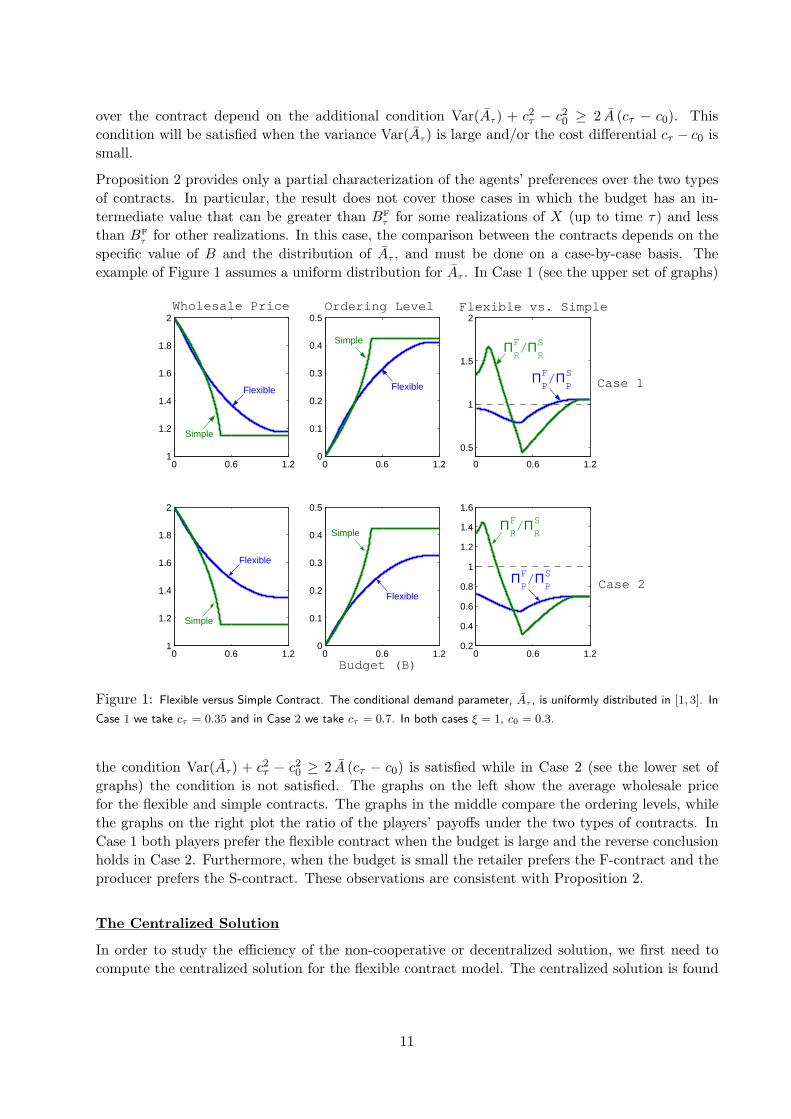
τ for other realizations. In this case, the comparison between the contracts depends on thespecific value of B and the distribution of Aτ , and must be done on a case-by-case basis. Theexample of Figure 1 assumes a uniform distribution for Aτ . In Case 1 (see the upper set of graphs)

0 0.6 1.21

1.2

1.4

1.6

1.8

2Wholesale Price

0 0.6 1.20

0.1

0.2

0.3

0.4

0.5Ordering Level

0 0.6 1.2

0.5

1

1.5

2Flexible vs. Simple

0 0.6 1.21

1.2

1.4

1.6

1.8

2

0 0.6 1.20

0.1

0.2

0.3

0.4

0.5

Budget (B) 0 0.6 1.2

0.2

0.4

0.6

0.8

1

1.2

1.4

1.6

Case 1

Case 2

Flexible

Simple

Flexible

Simple

Flexible

Flexible

Simple

Simple

ΠRF/Π

RS

ΠRF/Π

RS

ΠPF/Π

PS

ΠPF/Π

PS

Figure 1: Flexible versus Simple Contract. The conditional demand parameter, Aτ , is uniformly distributed in [1, 3]. In

Case 1 we take cτ = 0.35 and in Case 2 we take cτ = 0.7. In both cases ξ = 1, c0 = 0.3.

the condition Var(Aτ) + c2τ − c2

0 ≥ 2 A (cτ − c0) is satisfied while in Case 2 (see the lower set ofgraphs) the condition is not satisfied. The graphs on the left show the average wholesale pricefor the flexible and simple contracts. The graphs in the middle compare the ordering levels, whilethe graphs on the right plot the ratio of the players’ payoffs under the two types of contracts. InCase 1 both players prefer the flexible contract when the budget is large and the reverse conclusionholds in Case 2. Furthermore, when the budget is small the retailer prefers the F-contract and theproducer prefers the S-contract. These observations are consistent with Proposition 2.

The Centralized Solution

In order to study the efficiency of the non-cooperative or decentralized solution, we first need tocompute the centralized solution for the flexible contract model. The centralized solution is found

11

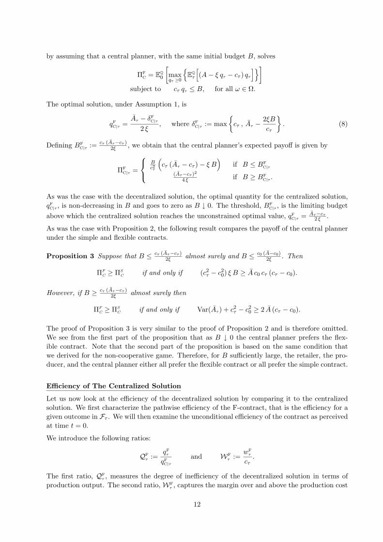
by assuming that a central planner, with the same initial budget B, solves

ΠFC = EQ0

[maxqτ ≥0

EQτ

[(A− ξ qτ − cτ ) qτ

]]

subject to cτ qτ ≤ B, for all ω ∈ Ω.

The optimal solution, under Assumption 1, is

qFC|τ =

Aτ − δFC|τ

2 ξ, where δF

C|τ := max

cτ , Aτ − 2ξB

cτ

. (8)

Defining BFC|τ := cτ (Aτ−cτ )

2ξ , we obtain that the central planner’s expected payoff is given by

ΠFC|τ =

Bc2τ

(cτ (Aτ − cτ )− ξ B

)if B ≤ BF

C|τ(Aτ−cτ )2

4 ξ if B ≥ BFC|τ .

As was the case with the decentralized solution, the optimal quantity for the centralized solution,qFC|τ , is non-decreasing in B and goes to zero as B ↓ 0. The threshold, BF

C|τ , is the limiting budgetabove which the centralized solution reaches the unconstrained optimal value, qF

C|τ = Aτ−cτ2 ξ .

As was the case with Proposition 2, the following result compares the payoff of the central plannerunder the simple and flexible contracts.

Proposition 3 Suppose that B ≤ cτ (Aτ−cτ )2ξ almost surely and B ≤ c0 (A−c0)

2ξ . Then

ΠFC ≥ ΠS

C if and only if (c2τ − c2

0) ξ B ≥ A c0 cτ (cτ − c0).

However, if B ≥ cτ (Aτ−cτ )2ξ almost surely then

ΠFC ≥ ΠS

C if and only if Var(Aτ) + c2τ − c2

0 ≥ 2 A (cτ − c0).

The proof of Proposition 3 is very similar to the proof of Proposition 2 and is therefore omitted.We see from the first part of the proposition that as B ↓ 0 the central planner prefers the flex-ible contract. Note that the second part of the proposition is based on the same condition thatwe derived for the non-cooperative game. Therefore, for B sufficiently large, the retailer, the pro-ducer, and the central planner either all prefer the flexible contract or all prefer the simple contract.

Efficiency of The Centralized Solution

Let us now look at the efficiency of the decentralized solution by comparing it to the centralizedsolution. We first characterize the pathwise efficiency of the F-contract, that is the efficiency for agiven outcome in Fτ . We will then examine the unconditional efficiency of the contract as perceivedat time t = 0.

We introduce the following ratios:

QFτ :=

qFτ

qFC|τ

and WFτ :=

wFτ

cτ.

The first ratio, QFτ , measures the degree of inefficiency of the decentralized solution in terms of

production output. The second ratio, WFτ , captures the margin over and above the production cost

12

charged by the producer. Naturally, WFτ ≥ 1 and so it follows that QF

τ ≤ 1. This inefficiency ofthe decentralized solution has been long recognized in the economics literature and goes under thename of double marginalization (e.g., Spengler 1950). We characterize these performance ratioshere in the context of a budget constraint.

By Corollary 1, the double marginalization ratio, WFτ , is a non-increasing function of B and satisfies

limB↓0WFτ = Aτ

cτ. The ratio, QF

τ , satisfies

QFτ =

cτ

Aτ−

√A2

τ−8 ξ B

4 ξ B if B ≤ BFC|τ ∧BF

τ

Aτ−√

A2τ−8 ξ B

2 (Aτ−cτ )if BF

C|τ ≤ B ≤ BFτ

cτ (Aτ−cτ )4 ξ B if BF

C|τ ≤ B ≤ BFτ

12 if B ≥ BF

C|τ ∨BFτ

where x ∨ y := maxx, y and x ∧ y := minx, y.Depending on the values of the average market size, Aτ , and production cost, cτ , either BF

C|τ ≥ BFτ

or BFC|τ ≤ BF

τ . For this reason we have to distinguish four possible cases in the computation of QFτ

as above. It is straightforward to show that BFC|τ ≤ BF

τ if and only if Aτ ≤ 3 cτ .

The monotonicity of WFτ implies that QF

τ increases in B in the range B ∈ [0, BFC|τ ∧ BF

τ ]. Withinthis range, smaller budgets therefore hurt the efficiency of the supply chain with respect to thecentralized solution more than larger budgets. In the limit we obtain

limB↓0

QFτ =

cτ

Aτ

.

For B ≥ BFC|τ ∨BF

τ , however, the ratio QFτ remains constant at 1

2 .

In the range BFC|τ∧BF

τ ≤ B ≤ BFC|τ∨BF

τ , the behavior ofQFτ is different depending on the relationship

between BFC|τ and BF

τ . If BFC|τ ≤ BF

τ then QFτ is increasing in B. If BF

τ ≤ BFC|τ then QF

τ is decreasingin B. In both cases, however, the double marginalization inefficiency is minimized at B = BF

τ .

To analyze the overall efficiency of the F-contract we look at the competition penalty, PFτ , (e.g.,

Cachon and Zipkin 1999) which is defined as

PFτ := 1−

(ΠF

R|τ + ΠFP|τ

ΠFC|τ

).

It is clear that PFτ ∈ [0, 1] with PF

τ = 0 implying that the decentralized chain is perfectly coordinatedand achieving the same expected profit as the centralized system. When PF

τ = 1, however, thesystem is completely inefficient. In our setting, we can write the competition penalty as follows:

PFτ = 1−

(Aτ − cτ − ξ qF

τ

Aτ − cτ − ξ qFC|τ

)QF

τ .

Proposition 4 The competition penalty, as a function of B, is characterized as follows:

PFτ =

decreases in B if B ≤ BFC|τ ∧BF

τ

decreases in B if BFC|τ ≤ B ≤ BF

τ

increases in B if BFτ ≤ B ≤ BF

C|τ

14 if B ≥ BF

C|τ ∨BFτ .

13

Proof: The proof is straightforward and is therefore omitted.

Figure 2 summarizes the solution for the F-contract for a given realization in Fτ . The graphson the top row correspond to the case BF

C|τ ≤ BFτ while those on the bottom row correspond to

BFτ ≤ BF

C|τ . The graphs on the left plot the quantity ratio, QFτ , the graphs in the middle plot the

double marginalization ratio, WFτ , and the graphs on the right plot the competition penalty, PF

τ .In the case BF

τ ≤ BFC|τ , or equivalently Aτ ≤ 3 cτ , the competition penalty is minimized at B = BF

τ

0 0.5 10.3

0.35

0.4

0.45

0.5

0.55

0 0.5 12

2.5

3

3.5

0 0.5 10.2

0.3

0.4

0.5

0.6

0.7

0 0.5 10.45

0.5

0.55

0.6

0.65

0.7

0.75

0.8

0 0.5 11.3

1.4

1.5

1.6

1.7

1.8

0 0.5 10.15

0.2

0.25

0.3

0.35

0.4

Budget (B)

QFτ WFτ PFτ

BFC|τ ≤ BFτ

BFτ ≤ BFC|τ

Figure 2: QFτ , WF

τ and PFτ are plotted against B for the flexible contract. The demand model is such that Aτ = 2 and

ξ = 1. The production cost is cτ = 0.6 for the top row and cτ = 1.2 for the bottom row.

and takes the value

PFmin|X =

(5 cτ − Aτ) (Aτ − cτ )(Aτ + cτ ) (7 cτ − Aτ)

≤ 14.

If Aτ = cτ note that the competition penalty vanishes but this is only due to the fact that q = 0for both the decentralized and centralized supply chains.

Thus far, the efficiency of the F-contract has been discussed in a pathwise fashion, that is conditionalon Fτ . We now consider the unconditional efficiency. In particular, we are interested in charac-terizing the expected production efficiency, QF := EQ0[QF

τ ], the expected double marginalization,WF := EQ0[WF

τ ], and the expected competition penalty, PF := EQ0 [PFτ ].

The computation of these quantities follows directly from our previous analysis though the com-putations are rather tedious due to the number of different cases that arise in terms of B, BF

τ , andBF

C|τ . The following proposition summarizes the unconditional efficiency of the F-contract in thelimiting cases B ↓ 0 and B ↑ ∞.

14

Proposition 5 In the limit as the budget, B, goes to 0 we obtain

limB↓0

QF = EQ[cτ

Aτ

] ≥ cτ

A, lim

B↓0WF =

A

cτ, and lim

B↓0PF = 1− EQ[ cτ

Aτ

] ≤ A− cτ

A.

As B →∞ we obtain

limB↑∞

QF =12, lim

B↑∞WF =

A + cτ

2cτ, and lim

B↑∞PF =

14.

Proof: The proof follows from the nonnegativity of Aτ , the bounded convergence theorem, andJensen’s inequality.

Proposition 5 implies that for B ↓ 0 or B ↑ ∞ the expected double marginalization, WF, decreaseswith τ . That is, production postponement reduces, on average, the producer’s margin. On the otherhand, the competition penalty is maximized at τ = 0 for B small and it is constant, independentof τ , for B large.

4 Flexible Contract with Financial Hedging

We now consider the H-contract, that is the flexible contract but where the retailer now has accessto the financial markets. The complete financial markets assumption implies that the retailer canmodify his budget by purchasing any Fτ -measurable financial claim, Gτ , where, as usual, Ft0≤t≤T

is the filtration generated by the financial noise, Xt. Assuming without loss of generality15 thatan initial capital of 0 is devoted to the financial hedging strategy, we then have EQ0 [Gτ ] = 0. Theretailer’s budget at time τ is then given by Bτ = B + Gτ . By optimizing over Gτ , the retailer cantransfer cash resources from states where the budget constraint is not binding to states where itis. In a partial equilibrium setting, that is for a fixed wτ , it is clear that the retailer will prefer theH-contract to the F-contract. In our competitive setting, however, this is no longer clear. In fact weshall see that on some occasions the retailer will prefer the H-contract but on other occasions he willprefer the F-contract. We shall see that the producer, however, will always prefer the H-contractto the F-contract.

The Decentralized Solution

The sequence of events in the H-contract setting is as follows. At time t = 0, the producer offersa menu of wholesale prices, wτ . In response, the retailer selects a menu of ordering quantities,qτ = q(wτ ), as well as an Fτ -measurable financial claim, Gτ , that satisfies EQ0 [Gτ ] = 0. At timeτ the outcome is observed and the producer immediately manufactures qτ product units which hethen sells to the retailer at a per unit price of wτ . By construction, the retailer’s budget, Bτ , issufficient to pay the producer for these units. Finally, the retailer sells all the units in the retailmarket at time T at the stochastic per-unit clearance price, A− ξ qτ .

The distinguishing feature of the H-contract is that the budget constraint is now a path-wiseconstraint of the form

wτ qτ ≤ Bτ , for all ω ∈ Ω15See Section 2.3.

15

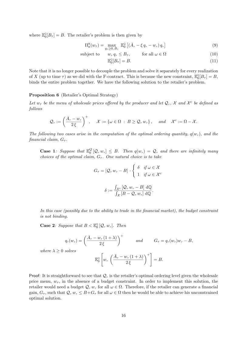
where EQ0[Bτ ] = B. The retailer’s problem is then given by

ΠHR(wτ ) = max

qτ≥0, Bτ

EQ0[(Aτ − ξ qτ − wτ) qτ

](9)

subject to wτ qτ ≤ Bτ , for all ω ∈ Ω (10)

EQ0[Bτ ] = B. (11)

Note that it is no longer possible to decouple the problem and solve it separately for every realizationof X (up to time τ) as we did with the F-contract. This is because the new constraint, EQ0[Bτ ] = B,binds the entire problem together. We have the following solution to the retailer’s problem.

Proposition 6 (Retailer’s Optimal Strategy)

Let wτ be the menu of wholesale prices offered by the producer and let Qτ , X and X c be defined asfollows

Qτ :=(

Aτ − wτ

2 ξ

)+

, X := ω ∈ Ω : B ≥ Qτ wτ , and X c := Ω−X .

The following two cases arise in the computation of the optimal ordering quantity, q(wτ), and thefinancial claim, Gτ .

Case 1: Suppose that EQ0 [Qτ wτ ] ≤ B. Then q(wτ) = Qτ and there are infinitely many

choices of the optimal claim, Gτ . One natural choice is to take

Gτ = [Qτ wτ −B] ·

δ if ω ∈ X1 if ω ∈ X c

δ :=

∫X c [Qτ wτ −B] dQ∫X [B −Qτ wτ ] dQ

.

In this case (possibly due to the ability to trade in the financial market), the budget constraintis not binding.

Case 2: Suppose that B < EQ0 [Qτ wτ ]. Then

qτ(wτ) =(

Aτ − wτ (1 + λ)2 ξ

)+

and Gτ = qτ(wτ)wτ −B,

where λ ≥ 0 solves

EQ0

[wτ

(Aτ − wτ (1 + λ)

2 ξ

)+]

= B.

Proof: It is straightforward to see that Qτ is the retailer’s optimal ordering level given the wholesaleprice menu, wτ , in the absence of a budget constraint. In order to implement this solution, theretailer would need a budget Qτ wτ for all ω ∈ Ω. Therefore, if the retailer can generate a financialgain, Gτ , such that Qτ wτ ≤ B+Gτ for all ω ∈ Ω then he would be able to achieve his unconstrainedoptimal solution.

16

By definition, X contains all those states for which B ≥ Qτ wτ . That is, the original budget B islarge enough to cover the optimal purchasing cost for all ω ∈ X . However, for ω ∈ X c, the initialbudget is not sufficient. The financial gain, Gτ , then allows the retailer to transfer resources fromX to X c.

Suppose the condition in Case 1 holds so that EQ0 [Qτ wτ ] ≤ B. Note that according to the definitionof Gτ in this case, we see that B + Gτ = Qτ wτ for all ω ∈ X c. For ω ∈ X , however, B + Gτ =(1 − δ) B + δQτ wτ ≥ Qτ wτ . The inequality follows since δ ≤ 1. Gτ therefore allows the retailerto implement the unconstrained optimal solution. The only point that remains to check is that Gτ

satisfies EQ0 [Gτ ] = 0. This follows directly from the definition of δ.

Suppose now that the condition specified in Case 2 holds. We solve the retailer’s optimizationproblem in (9) by relaxing the gain constraint (11) with a Lagrange multiplier, λ. We also relax thebudget constraint in (10) for each realization of X up to time τ . The corresponding multiplier foreach such realization is denoted by βτ dQ where βτ plays the role of a Radon-Nikodym derivativeof a positive measure that is absolutely continuous with respect to Q. The first-order optimalityconditions for the relaxed version of the retailer’s problem are then given by

qτ =(Aτ − wτ (1 + βτ))+

2 ξ

βτ = λ, βτ

(wτ qτ −B + Gτ

)= 0, βτ ≥ 0, and EQ0[Gτ ] = 0.

It is straightforward to show that the solution given in Case 2 of the proposition satisfies theseoptimality conditions; only the non-negativity of βτ needs to be checked separately. To prove this,note that βτ = λ, therefore it suffices to show that λ ≥ 0. This follows from three observations

(a) Since 0 ≤ wτ the function EQ0

[wτ

(Aτ−wτ (1+λ)

2 ξ

)+]

is decreasing in λ.

(b) In Case 2, by hypothesis, we have

EQ0

[wτ

(Aτ − wτ

2 ξ

)+]

= EQ0 [Qτ wτ ] > B

(c) Finally, we know that λ solves

EQ0

[wτ

(Aτ − wτ (1 + λ)

2 ξ

)+]

= B.

(a) and (b) therefore imply that we must have λ ≥ 0. ¤

Case 1 of Proposition 6 describes the circumstances when trading in the financial market allows theretailer to completely remove the budget constraint from his optimization problem. When thesecircumstances are not satisfied as in Case 2, the retailer cannot completely remove the budgetconstraint. He can, however, mitigate the effects of the budget constraint somewhat so that for afixed menu of wholesale prices, wτ , he prefers the H-contract to the F-contract.

17

Based on the retailer’s best-response strategy derived in Proposition 6, the producer’s problem canbe formulated16 as

ΠHP = max

wτ , λ≥0EQ0

[(wτ − cτ )

(Aτ − wτ (1 + λ)

2 ξ

)+]

(12)

subject to EQ0

[wτ

(Aτ − wτ (1 + λ)

2 ξ

)+]≤ B. (13)

The following result characterizes the solution of this problem and the corresponding solution ofthe Stackelberg game.

Proposition 7 (Producer’s Optimal Strategy and the Stackelberg Solution)

Let φH be the minimum φ ≥ 1 that solves

EQ0

[(A2

τ − (φ cτ )2

8 ξ

)+]≤ B.

Define δH := φH cτ , then the optimal wholesale price and ordering level satisfy

wHτ =

Aτ + δH

2and qH

τ =(

Aτ − δH

4 ξ

)+

. (14)

The players’ expected payoffs satisfy

ΠHP|τ =

(Aτ + δH − 2cτ ) (Aτ − δH)+

8 ξand ΠH

R|τ =((Aτ − δH)+)2

16 ξ. (15)

Proof: See Appendix A.

As before, we interpret δH as a modified production cost, greater than or equal to the the originalcost, cτ , that is imposed in the supply chain because of the limited budget. Unlike the settingof the F-contract, however, the modified cost in this setting is not stochastic. Note that δH isnondecreasing in B. Hence, as in the F-contract, the more cash constrained the retailer is thehigher the wholesale price charged by the producer.

Suppose now that the budget is limited so that δH > cτ . Then, depending on the value of δH,Proposition 7 implies that it is possible for wH

τ ≥ Aτ and qHτ = 0 for some outcomes ω ∈ Ω. That

is, in some cases the producer decides to overcharge the retailer and therefore make the supplychain nonoperative. Because of Assumption 1, this behavior was never optimal in the setting ofthe F-contract. It occurs in the H-contract setting, however, because the retailer can allocate hislimited budget among different states ω ∈ Ω. In particular, if the retailer knows that for someoutcomes, ω, he will not be purchasing any units then he can transfer the entire budget B fromthese (non-operative) states to states in which there is a need for cash. It is in the producer’sinterest, then, to select those states in which he wants to do business with the retailer and thosein which he does not. Note that qH

τ = 0 if and only if Aτ ≤ δH. Hence the producer “closes” thesupply chain when the forecasted demand is low.

We now compare the F-contract with the H-contract in terms of the players expected payoffs underthe Nash equilibrium. First we define

X := ω ∈ Ω : δFτ = cτ

16Note that at the optimal solution, the constraint in (13) will be tight if the optimal λ is greater than zero. This

will only occur when the budget constraint is binding.

18

where δFτ was defined in proposition 1 in Section 3. The set X characterizes those states, ω, for which

the flexible contract achieves the unconstrained optimal solution, wFτ = Aτ+cτ

2 and qFτ = Aτ−cτ

4ξ . Wealso recall that the equilibrium wholesale prices and ordering levels for the F-contract and H-contract are

wFτ =

Aτ + δFτ

2qF

τ =Aτ − δF

τ

4 ξand wH

τ =Aτ + δH

2qH

τ =(Aτ − δH)+

4 ξ,

respectively. The difference between the expected payoffs of these two contracts depends on thedifference between δF

τ and δH, which in turn depends on the set X . We now show that the producer’sexpected payoff under the H-contract is always greater than his expected payoff under the F-contract.

Proposition 8 The producer is always better-off if the retailer is able to hedge the budget con-straint.

Proof: See Appendix A.

According to this result, it is in the producer’s interest to promote the retailer’s ability to trade inthe financial market. If the retailer is a small player with limited access to the financial markets,then it would be in the producer’s interest to serve as an intermediary between the retailer and thefinancial markets.

¿From the retailer’s perspective, the comparison between the F-contract and H-contract is not sostraightforward. We identify three cases.

• Case 1: Suppose that X = Ω. In this case, B is sufficiently large so that δFτ = δH = cτ for all

ω ∈ Ω and the two contracts produce the same output. This is not surprising since for largebudgets financial trading does not offer any advantage.

• Case 2: Suppose that X 6= Ω and δH = cτ . In this case, δFτ > cτ for all ω ∈ X c. Therefore,

wHτ ≤ wF

τ and qHτ ≥ qF

τ for all ω ∈ Ω with strict inequalities in X c. With regards to the payoffs,using equations (7) and (15) we can conclude that for all ω ∈ Ω

ΠHR|τ ≥ ΠF

R|τ ,

with strict inequality in X c. Note that this case summarizes well the advantages of usingfinancial trading: the ability to trade has increased the output of the supply chain, reducedthe wholesale price, reduced the double marginalization inefficiency and has increased thepayoff of both agents. These conclusions hold for all ω ∈ Ω in this case. Therefore, they holdin expectation, so that EQ0 [ΠH

R|τ ] ≥ EQ0 [ΠFR|τ ].

• Case 3: Suppose that X 6= Ω and δH > cτ . In this case, δFτ < δH for ω ∈ X and the wholesale

price (ordering quantity) is smaller (higher) under the F-contract than under the H-contract.In terms of payoffs, the retailer (and the producer as well) therefore prefers the F-contractto the H-contract for ω ∈ X . Of course, the choice of the contract has to be made at t = 0when the realization of ω is still unknown. Therefore, the appropriate comparison betweenthe contracts should be based on their time t = 0 expected payoffs. As the following exampleshows, however, the retailer can be better-off or worse-off under the H-contract.

19

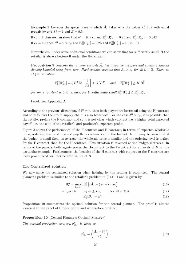
Example 1 Consider the special case in which Aτ takes only the values 5, 10 with equal

probability and 8 ξ = 1 and B = 9.5.

If cτ = 1 then we can show that δH = 9 > cτ and EQ0 [ΠHR|τ ] = 0.25 and EQ0 [ΠF

R|τ ] = 0.342.

If cτ = 4.5 then δH = 9 > cτ and EQ0 [ΠHR|τ ] = 0.25 and EQ0 [ΠF

R|τ ] = 0.122. ¤

Nevertheless, under some additional conditions we can show that for sufficiently small B theretailer is always better-off under the H-contract.

Proposition 9 Suppose the random variable Aτ has a bounded support and admits a smoothdensity bounded away from zero. Furthermore, assume that Aτ > cτ for all ω ∈ Ω. Then, asB ↓ 0 we obtain

EQ0 [ΠFR|τ ] = ξ B2 EQ0

[1

A2τ

]+ O

(B3

)and EQ0 [Π

HR|τ ] ≥ K B

32

for some constant K > 0. Hence, for B sufficiently small EQ0 [ΠFR|τ ] ≤ EQ0[ΠH

R|τ ].

Proof: See Appendix A.

According to the previous discussion, if δH = cτ then both players are better-off using the H-contractand so it follows the entire supply chain is also better-off. For the case δH > cτ , it is possible thatthe retailer prefers the F-contract and so it is not clear which contract has a higher total expectedpayoff, i.e. the sum of the retailer’s and producer’s expected profits.

Figure 3 shows the performance of the F-contract and H-contract, in terms of expected wholesaleprice, ordering level and players’ payoffs, as a function of the budget, B. It may be seen that ifthe budget is small then, on average, the wholesale price is smaller and the ordering level is higherfor the F-contract than for the H-contract. This situation is reversed as the budget increases. Interms of the payoffs, both agents prefer the H-contract to the F-contract for all levels of B in thisparticular example. Furthermore, the benefits of the H-contract with respect to the F-contract aremost pronounced for intermediate values of B.

The Centralized Solution

We now solve the centralized solution when hedging by the retailer is permitted. The centralplanner’s problem is similar to the retailer’s problem in (9)-(11) and is given by

ΠHC = max

qτ , Bτ

EQ0[(Aτ − ξ qτ − cτ ) qτ

](16)

subject to wτ qτ ≤ Bτ , for all ω ∈ Ω (17)

EQ0[Bτ ] = B. (18)

Proposition 10 summarizes the optimal solution for the central planner. The proof is almostidentical to the proof of Proposition 6 and is therefore omitted.

Proposition 10 (Central Planner’s Optimal Strategy)

The optimal production strategy, qHC|τ , is given by

qHC|τ =

(Aτ − δH

C

2 ξ

)+

(19)

20

0 0.5 1 1.5 2

1.2

1.4

1.6

1.8

2

2.2

2.4

Wholesale Price

Budget (B)0 0.5 1 1.5 2

0

0.05

0.1

0.15

0.2

0.25

0.3

0.35

0.4Ordering Level

0 0.5 1 1.5 20

0.05

0.1

0.15

0.2

0.25

0.3

0.35Producer’s Payoff

0 0.5 1 1.5 20

0.02

0.04

0.06

0.08

0.1

0.12

0.14

0.16

0.18Retailer’s Payoff

Budget (B)

Budget (B)Budget (B)

H−Contract

F−Contract

H−Contract

F−Contract

F−Contract F−Contract

H−Contract

H−Contract

Figure 3: Performance of F-contract and H-contract as a function of the budget. The demand parameter Aτ is uniformly

distributed in [1, 3], ξ = 1, and cτ = 0.5.

where δHC is the minimum δ ≥ cτ that solves

EQ[cτ

(Aτ − δH

C

2 ξ

)+]≤ B.

The central planner’s optimal payoff given the information available at time τ is

ΠHC|τ =

(Aτ + δHC − 2cτ ) (Aτ − δH

C)+

4 ξ. (20)

Once again, we interpret δHC as a modified production cost induced by the budget constraint.

Efficiency of The Centralized Solution

With this modified production cost structure in mind, one would expect the centralized solution tobe more efficient than the decentralized solution in the sense that δH

C ≤ δH. This is not always thecase, however, as the following example demonstrates.

Example 2 Consider the following instance of the problem with B = 0.45, ξ = cτ = 1, and Aτ

uniformly distributed in [1, 3]. Since

EQ0

[(A2

τ − c2τ

8ξ

)+]

=512

< B and EQ0

[cτ

(Aτ − cτ

2ξ

)]=

12

> B,

21

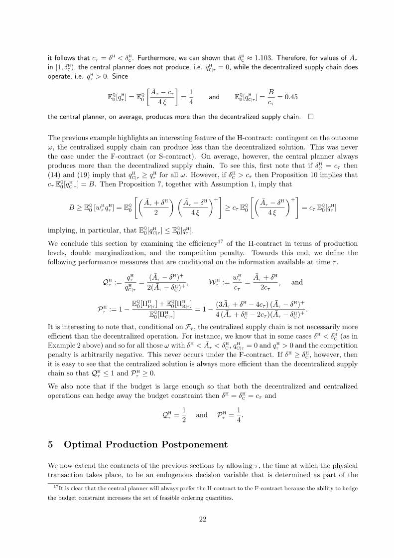
it follows that cτ = δH < δHC . Furthermore, we can shown that δH

C ≈ 1.103. Therefore, for values of Aτ

in [1, δHC ), the central planner does not produce, i.e. qH

C|τ = 0, while the decentralized supply chain does

operate, i.e. qHτ > 0. Since

EQ0[qHτ ] = EQ0

[Aτ − cτ

4 ξ

]=

14

and EQ0 [qHC|τ ] =

B

cτ= 0.45

the central planner, on average, produces more than the decentralized supply chain. ¤

The previous example highlights an interesting feature of the H-contract: contingent on the outcomeω, the centralized supply chain can produce less than the decentralized solution. This was neverthe case under the F-contract (or S-contract). On average, however, the central planner alwaysproduces more than the decentralized supply chain. To see this, first note that if δH

C = cτ then(14) and (19) imply that qH

C|τ ≥ qHτ for all ω. However, if δH

C > cτ then Proposition 10 implies thatcτ EQ0 [qH

C|τ ] = B. Then Proposition 7, together with Assumption 1, imply that

B ≥ EQ0 [wHτ qH

τ ] = EQ0

[(Aτ + δH

2

) (Aτ − δH

4 ξ

)+]≥ cτ EQ0

[(Aτ − δH

4 ξ

)+]

= cτ EQ0 [qHτ ]

implying, in particular, that EQ0 [qHC|τ ] ≤ EQ0[qH

τ ].

We conclude this section by examining the efficiency17 of the H-contract in terms of productionlevels, double marginalization, and the competition penalty. Towards this end, we define thefollowing performance measures that are conditional on the information available at time τ .

QHτ :=

qHτ

qHC|τ

=(Aτ − δH)+

2(Aτ − δHC)+

, WHτ :=

wHτ

cτ=

Aτ + δH

2cτ, and

PHτ := 1− E

Q0[Π

HP|τ ] + EQ0 [ΠH

R|τ ]EQ0 [ΠH

C|τ ]= 1− (3Aτ + δH − 4cτ ) (Aτ − δH)+

4 (Aτ + δHC − 2cτ )(Aτ − δH

C)+.

It is interesting to note that, conditional on Fτ , the centralized supply chain is not necessarily moreefficient than the decentralized operation. For instance, we know that in some cases δH < δH

C (as inExample 2 above) and so for all those ω with δH < Aτ < δH

C , qHC|τ = 0 and qH

τ > 0 and the competitionpenalty is arbitrarily negative. This never occurs under the F-contract. If δH ≥ δH

C , however, thenit is easy to see that the centralized solution is always more efficient than the decentralized supplychain so that QH

τ ≤ 1 and PHτ ≥ 0.

We also note that if the budget is large enough so that both the decentralized and centralizedoperations can hedge away the budget constraint then δH = δH

C = cτ and

QHτ =

12

and PHτ =

14.

5 Optimal Production Postponement

We now extend the contracts of the previous sections by allowing τ , the time at which the physicaltransaction takes place, to be an endogenous decision variable that is determined as part of the

17It is clear that the central planner will always prefer the H-contract to the F-contract because the ability to hedge

the budget constraint increases the set of feasible ordering quantities.

22

solution to the Nash equilibrium. We discuss this problem initially in the context of the H-contractbut later we will assume that B is sufficiently large so that the analysis of the F-contract is thesame as that of the H-contract.

We consider two alternatives formulations. In the first alternative, τ is restricted to be a deter-ministic time in [0, T ] that is selected at time t = 0. Motivated by the terminology of dynamicprogramming, we refer to this alternative as the optimal open-loop production postponement model.In the second alternative, we permit τ to be an Ft-stopping time that is bounded above by T . Wecall this alternative the optimal closed-loop production postponement model. In both cases, theprocurement contract offered by the producer takes the form of a pair, (τ, wτ), where the whole-sale price menu, wτ , is required to be Fτ -measurable. We note that the producer always prefersthe closed-loop model though from a practical standpoint the open-loop model may be easier toimplement in practice.

Independently of whether τ is a deterministic time or a stopping time, the optimal ordering level forthe retailer, given a contract (τ, wτ ), is an Fτ -measurable menu, qτ , that satisfies18 the conditionsin Proposition 6. The producer’s problem is therefore given by (12) and (13) but now with τ as anextra decision variable. Furthermore, since the proof of Proposition 7 (see the Appendix) extendsto the case of a stopping time, we conclude that the optimal wholesale price menu, wτ , as a functionof τ is still given by equation (14). In summary, the producer’s problem of selecting the optimaltime τ is given by

ΠHP = max

τ,φ≥1EQ0

[(Aτ + φ cτ − 2cτ ) (Aτ − φ cτ )+

8 ξ

](21)

subject to EQ0

[(A2

τ − φ2 c2τ

8 ξ

)+]≤ B. (22)

Of course τ should be restricted to either a deterministic time or a stopping time depending onwhich model (open-loop or closed-loop) is under consideration. For a given τ , the objective in (21)is decreasing in φ so that the producer’s problem reduces to

ΠHP = max

τEQ0

[(Aτ + φ cτ − 2cτ ) (Aτ − φ cτ )+

8 ξ

](23)

subject to φ = inf

ψ ≥ 1 : EQ0

[(A2

τ − ψ2 c2τ

8 ξ

)+]≤ B

. (24)

To solve this optimization problem we would first need to specify the functional forms of Aτ andcτ and depending on these specifications, the solution may or may not be easy to find. For theremainder of this section, however, we will show how this problem may be solved when additionalassumptions are made. In particular, we make the following three assumptions:

1. Xt is a diffusion process with dynamics satisfying

dXt = σ(Xt) dWt, (25)

where Wt a Q-Brownian motion. Note that we have not included a drift term in the dynamicsof Xt since it must be the case that Xt is a Q-martingale. This is not a significant assumptionand we could easily consider alternative processes for Xt.

18It is easy to check that the proof of Proposition 6 remains unchanged if τ is allowed to be a stopping time.

23

2. We adopt a specific functional form to model the dependence between the market clearanceprice and the financial market. In particular, we assume that there behaves a well-behaved19

function, F (x), and a random variable, ε, such that one of the following two models holds.

Additive Model: A = F (XT ) + ε, with EQ[ε] = 0, or (26)

Multiplicative Model: A = ε F (XT ), with ε ≥ 0 and EQ[ε] = 1. (27)

The random perturbation ε captures the non-financial component of the market price uncer-tainty and is assumed to be independent of Xt. Note that if F (x) = A, we recover a modelfor which demand is independent of the financial market.

3. We assume that the initial budget, B, is sufficiently large so that the retailer is able to hedgeaway the budget constraint for every stopping time, τ . That is, φ = 1 for every τ ∈ T . Forexample, if τ ≡ 0 then there is no time for hedging to take place and so it is necessary that B isat least sufficiently large so that the budget constraint is not binding for the simple contract.This is a significant assumption20 and effectively reduces the problem to one of finding theoptimal (random) timing of the flexible contract when there is no budget constraint.

5.1 Optimal Open-Loop Production Postponement

We now restrict τ to be a deterministic time in [0, T ]. Based on the third assumption above, theproducer’s optimization problem in (23) reduces to

maxτ∈[0,T ]

EQ0[(Aτ − cτ )2

]= max

τ∈[0,T ]Var(Aτ) + (A− cτ )2. (28)

We note that in this optimization problem there is a trade-off between demand learning as repre-sented by the variance term, Var(Aτ), and production costs as represented by (A− cτ )2. The firstterm is increasing in τ while the second term is decreasing in τ so that, in general, the optimiza-tion problem in (28) does not admit a trivial solution and depends on the particular form of thefunctions Var(EQ[A |Xτ ]) and cτ .

The Ito Representation Theorem (e.g. Øksendal 1998) implies the existence of an Ft-adaptedprocess, θt : t ∈ [0, T ], such that

A = A +∫ T

0θt dXt + ε or A = ε

(A +

∫ T

0θt dXt

)

for the additive or multiplicative model, respectively. In both cases the Q-martingale property ofXt implies

Aτ = A +∫ τ

0θt dXt. (29)

In order to compute the variance of Aτ we use the Q-martingale property of the stochastic integraland invoke Ito’s isometry (e.g. Øksendal 1998) to obtain

Var(Aτ) = EQ0

[(∫ τ

0θt dXt

)2]

= EQ0

[∫ τ

0θ2t d[X]t

],

19It is necessary, for example, that F (·) satisfy certain integrability conditions so that the stochastic integral in

(29) be a Q-martingale. In order to apply Ito’s Lemma it is also necessary to assume that F (·) is twice differentiable.

Because this section is intended to be brief, we omit the various technical conditions that are required to make our

arguments completely rigorous.20If we only wanted to solve for the open-loop policy it would not be necessary to make this assumption. In that

case we could solve for the optimal τ and φ in (23) and (24) numerically.

24

where the process [X]t is the quadratic variation of Xt with dynamics

d[X]t = σ2(Xt) dt.

It follows thatVar(Aτ) =

∫ τ

0EQ0[(θt σ(Xt))2] dt.

The open-loop optimal problem therefore reduces to solving

maxτ∈[0,T ]

∫ τ

0EQ0[(θt σ(Xt))2] dt + (A− cτ )2

. (30)

If there is an interior solution to this problem (i.e., τ∗ ∈ (0, T )), then it must satisfy the first-orderoptimality condition

EQ0 [(θτ σ(Xτ ))2]− 2 (A− cτ ) cτ = 0, where cτ :=dcτ

dτ.

Example 3 Consider the case in which the security price, Xt, follows a geometric Brownian motion

with dynamics

dXt = σ Xt dWt

where σ 6= 0 and Wt is a Q-Brownian motion. The quadratic variation process then satisfies d[X]t =σ2 X2

t dt. To model the dependence between the market clearance price and the process, Xt, we assume

a linear model for F (·) so that F (X) = A0 +A1 X where A0 and A1 are positive constants. Therefore,

depending on whether we consider the additive or multiplicative model, we have

A = A0 + A1 XT + ε or A = ε (A0 + A1 XT ),

where ε is a zero-mean or unit-mean random perturbation, respectively, that is independent of the

process Xt. It follows that Aτ = A0 +A1 Xτ and A = EQ0[A] = A0 +A1 X0. In addition, it is clear that

θt is identically equal to A1 for all t ∈ [0, T ]. We assume that the per unit production cost increases

with time and is given by

cτ = c0 + α τκ, for all τ ∈ [0, T ],

where α and κ are positive constants.

To impose the additional constraint that Aτ ≥ cτ for all τ (Assumption 1), we restrict our choice of the

parameters A0, T , c0, κ, and α so that A0 ≥ c0 +α T κ. Since EQ0[X2t ] = X2

0 exp(σ2 t) the optimization

problem in (30) reduces to

maxτ∈[0,T ]

(A1 X0)2 (exp(σ2 τ)− 1) + (A− c0 − α τκ)2

].

In general, a closed form solution is not available unless κ = 0. This is a trivial case in which cτ is

constant and the optimal strategy is to postpone production until time T so that τ∗ = T . Figure 4

shows the value of the objective function as a function of τ for four different values of κ. The cost

functions are such that it becomes cheaper to produce as κ increases. Note that for κ ∈ 4, 8, it is

convenient to postpone production using a flexible contract. For the more expensive production cost

functions that occur when κ ∈ 0.25, 1, production postponement is not profitable and the simple

contract is preferred. ¤

25

0 0.2 0.4 0.6 0.8 1

5

5.5

6

6.5

7

7.5

8

8.5

Time (τ)

κ = 8

κ = 4 κ =1

κ = 0.25

Figure 4: Optimal open-loop production postponement for four different production cost functions parameterized by κ.

The other parameters are X0 = A1 = σ = T = 1, A0 = 2, c0 = 0.3 and α = 0.7.

5.2 Optimal Closed-Loop Production Postponement

Instead of selecting a fixed transaction time, τ , at t = 0, the producer now optimizes over the setof stopping times bounded above by T . In this case, the optimization problem in (23) reduces tothe following optimal stopping problem

maxτ∈T

EQ0[(Aτ − cτ )2

], (31)

where T is the set of Ft-adapted stopping times bounded above by T . Again, the third assumptionabove has resulted in this simplified form of the objective function. According to the modeling ofA in (26) or (27), it follows that v(τ, Xτ ) := Aτ = EQτ [F (XT )] is a Q-martingale that satisfies

v(t, x)∂t

+12

σ2(x)∂2v(t, x)

∂x2= 0, v(T, x) = F (x).

We define U to be the set (t, x) : Gg(t, x) > 0 where g(t, x) := (v(t, x)−ct)2 is the payoff functionand G is the generator

G :=∂

∂t+

12σ2(x)

∂2

∂x2.

We then obtainU =

(t, x) : (σ(x) vx(t, x))2 > 2(v(t, x)− ct) ct

,

where vx is the first partial derivative of v with respect to x. In general, the set U is a propersubset of the optimal continuation region for the stopping problem in (31). Computing the optimalstopping time analytically is a difficult task and is usually done numerically. However, if U turnsout to equal the entire state space then it is clear that it is always optimal to continue.

Example 3: (Continued)

Consider the setting of Example 3 but where now τ is a stopping time instead of a deterministic time.

For the linear function F (X) = A0 + A1 X, the auxiliary function v satisfies v(t, x) = A0 + A1 x, and

26

the region U is given by

U =(t, x) : (σ x A1)2 > 2(A0 + A1 x− ct) ct

.

Straightforward calculations allow us to rewrite U as

U =

(t, x) : x >

ct +√

c2t + 2σ2 (A0 − ct) ct

σ2 A1

.

Let us define the auxiliary function

ρ(t) :=ct +

√c2t + 2σ2 (A0 − ct) ct

σ2 A1.

Since U is a subset of the optimal continuation region, we know that it is never optimal to stop if

Xt > ρ(t). Of course, it is possible that Xt < ρ(t) and yet still be optimal to continue.

We solved for the optimal continuation region numerically by using a binomial model to approximate

the dynamics of Xt. In so doing, we can assess the quality of the (suboptimal) strategy that uses ρ(t) to

define the continuation region. Figure 5 shows the optimal continuation region and the threshold ρ(t)for four different cost functions. These cost function are given by cτ = c0 + α τκ with κ = 0.25, 1, 4,

and 8. When X(τ) is above the optimal threshold it is optimal to continue. The vertical dashed line

corresponds to the optimal open-loop deterministic time computed in Figure 4. For κ = 0.25 or κ = 1this optimal deterministic time equals 0 since X0 lies below the optimal threshold. For κ = 4 it equals

0.476, and for κ = 8 it equals 0.678.

Interestingly, for high values of κ the auxiliary threshold ρ(t) is a good approximation for the optimal

solution. However, as κ decreases the quality of the approximation deteriorates rapidly. Except for the

case where κ = 0.25, the optimal threshold increases with time. This reflects the fact that the producer

becomes more likely to stop and exercise the procurement contract as the end of the horizon approaches.

We conclude this example by computing the optimal expected payoff for the producer under both the

optimal open-loop policy and the optimal closed-loop policy.

κ Open-Loop Payoff Closed-Loop Payoff % Increase

0.25 7.29 7.29 0.0%

1 7.29 7.305 0.2%

4 7.71 7.99 3.7%

8 8.09 8.33 3.8%

Producer’s expected payoff for four different production cost functions parameterized by κ.

The other parameters are A1 = X0 = σ = T = 1, A0 = 2, c0 = 0.3, α = 0.7 and ξ = 1/8.

Naturally, the optimal stopping time (closed-loop) policy produces a higher expected payoff than the

optimal deterministic time (open-loop) policy. The improvement, however, is only a few percentage

points which might suggest that a simpler contract based on a deterministic time captures most of the

benefits of allowing τ to be a decision variable. In practice, of course, it would be necessary to model the

operations and financial markets more accurately and to calibrate the resulting model correctly before

such conclusions could be drawn. ¤

27

0 0.2 0.4 0.6 0.8 10

2

4

6

8

10

12

14

Time (τ)

X(

τ)

κ = 8

0 0.2 0.4 0.6 0.8 10

1

2

3

4

5

6

7

Time (τ)

X(

τ)

κ = 4

0 0.2 0.4 0.6 0.8 1

1

2

3

4

5

Time (τ)

X(

τ)

κ = 1

0 0.2 0.4 0.6 0.8 10

2

4

6

8

10

Time (τ)

X(

τ)

κ = 0.25

ρ(t) ρ(t)

ρ(t)

ρ(t)

Optimal Optimal

Optimal

Optimal

Figure 5: Optimal continuation region for four different manufacturing cost functions parameterized by κ. The other

parameters are A1 = X0 = σ = T = 1, A0 = 2, c0 = 0.3 and α = 0.7.

6 Extensions

It is easy to extend the basic model to more accurately reflect the manner in which financial mar-kets impact the profitability of operations. In this section we describe some of these extensions. Inparticular, we focus on extensions21 where foreign exchange rates, interest rates and the possibilityof default influence the profitability of the competitive supply chain. We will concentrate onlyon the setting of the H-contract as this is a more interesting and challenging setting than that ofthe F-contract. We will also assume that the transaction time, τ , is deterministic and is givenexogenously as in Sections 3 and 4.

Extension 1: Stochastic Interest Rates

We now assume that interest rates are stochastic and that the Q-dynamics of the short rate aregiven by the Vasicek22 model so that

drt = α(µ− rt) dt + σdWt (32)21It is straightforward to construct other interesting variations of the basic model.22See, for example, Shreve (2004) for a description of the Vasicek model and other related results that we use in

the sequel. While it is not necessary to restrict ourselves to a particular term structure model here, we have done so

in order to simplify the exposition.

28

where α, µ and σ are all positive constants and Wt is a Q-Brownian motion. The short-rate, rt,is the instantaneous continuously compounded risk-free interest rate that is earned at time t bythe ‘cash account’, i.e., cash placed in a deposit account. In particular, if $1 is placed in the cashaccount at time t then it will be worth exp

(∫ Tt rs ds

)at time T > t. It may be shown that the

time τ value of a zero-coupon-bond with face value $1 that matures at time T > τ satisfies

ZTτ := ea(T−τ)+b(T−τ)rτ (33)

where a(·) and b(·) are known deterministic functions. In particular, ZTτ is the appropriate discount

factor for discounting a known deterministic cash flow from time T to time τ < T .

Returning to our competitive supply chain, we assume as before that the retailer’s profits arerealized at time T ≥ τ and that the budget B is only available at that time. However, we alsoassume that the producer demands payment from the retailer at time τ when the transaction takesplace. This means that if τ < T , then the retailer will be forced to borrow against the capital B

that would only be available at time T . As a result, the retailer’s effective budget at time τ is givenby

B(rτ ) := BZTτ = Bea(T−τ)+b(T−τ)rτ .

As before, we assume that the stochastic clearance price, A− ξqτ ,, depends on the financial marketthrough the co-dependence of the random variable A, and the financial process, Xt. To simplifythe exposition, we could assume that Xt ≡ rt but this is not necessary. If Xt is a financial processother than rt, we simply need to redefine our definition of Ft0≤t≤T so that it represents thefiltration generated by Xt and rt. Before formulating the optimization problems of the retailer andthe producer we must adapt our definition of feasible Fτ -measurable financial gains, Gτ . Until thispoint we have insisted that any such Gτ must satisfy EQ0 [Gτ ] = 0, assuming as before that zeroinitial capital is devoted to the financial hedging strategy. This was correct when interest rateswere identically zero but now we must replace that condition with the new condition23

EQ0 [DτGτ ] = 0 (34)

where Dτ := exp(− ∫ τ

0 rs ds). The retailer’s problem for a given Fτ -measurable wholesale price,

wτ , is therefore given24 by

ΠHR(wτ ) = max

qτ≥0, Gτ

EQ0 [DT (AT − ξ qτ) qτ −Dτwτqτ ] (35)

subject to wτ qτ ≤ B(rτ ) + Gτ , for all ω ∈ Ω (36)

EQ0 [DτGτ ] = 0 (37)

and Fτ −measurability of qτ . (38)

Note that both DT and Dτ appear in the objective function (35) reflecting the times at which theretailer makes and receives payments. We also had to explicitly impose the constraint that qτ be

23Martingale pricing theory states that the time 0 value, G0, of the security that is worth Gτ at time τ (and does

not pay any intermediate cash-flows) satisfies G0/N0 = EQ0[Gτ/Nτ ] where Nt is the time t price of the numeraire

security. It is common to take the cash account as the numeraire security and this is the approach we have followed

in this paper. Until now, however, the value of the cash account at time t was always $1 since we assumed interest

rates were identically zero. We therefore had G0 = EQ0[Gτ ] and since we insisted G0 = 0 we obtained EQ0[Gτ ] = 0.

When interest rates are non-zero we still have N0 = 1 but now Nτ = expR τ

0rs ds

and so we obtain (34). In the

main text we take Dt = N−1t . See Shreve (2004) for a development of martingale pricing theory (or arbitrage pricing

theory as it more commonly known).24We write AT for A to emphasize the timing of the cash-flow.

29

Fτ -measurable. This was necessary25 because of the appearance of DT in the objective function.We can easily impose the Fτ -measurability of qτ by conditioning with respect to Fτ inside theexpectation appearing in (35). We then obtain

EQ0[Dτ

(AD

τ − ξτ qτ − wτ

)qτ

](39)

as our new objective function where ADτ := EQτ [DT AT ]/Dτ and ξτ := ξZT

τ . With this new objectivefunction it is no longer necessary to explicitly impose the Fτ -measurability of qτ .

While this problem (and the producer’s problem that follows) might appear to be more complicatedthan the corresponding problems of Section 4 they are in fact no more difficult to solve. We havethe following solution to the retailer’s problem. We omit the proof as it is very similar to the proofof Proposition 6.

Proposition 11 (Retailer’s Optimal Strategy)

Let wτ be an Fτ -measurable wholesale price offered by the producer and define Qτ :=(

ADτ −wτ

2 ξτ

)+.

This is the optimal ordering quantity in the absence of a budget constraint. The following two casesarise:

Case 1: Suppose EQ0 [DτQτwτ ] ≤ EQ0 [DτB(rτ )] = ZT0 B. Then q(wτ ) = Qτ and (possibly due

to the ability to trade in the financial market) the budget constraint is not binding.

Case 2: Suppose EQ0 [DτQτwτ ] > ZT0 B. Then

qτ =(

ADτ − wτ (1 + λ)

2ξτ

)+

(40)

where λ ≥ 0 solvesEQ0 [Dτwτqτ ] = EQ0 [B(rτ )Dτ ] = ZT

0 B. (41)

Given the retailer’s best response, the producer’s problem may now be formulated26 as

ΠHP = max

wτ , λ≥0EQ0

[Dτ (wτ − cτ )

(AD

τ − wτ (1 + λ)2 ξτ

)+]

(42)

subject to EQ0

[Dτwτ

(AD

τ − wτ (1 + λ)2 ξτ

)+]≤ ZT

0 B. (43)

The Nash equilibrium and solution of the producer’s problem is given by the following proposition.We again omit the proof of this proposition as it it very similar to the proof of Proposition 7.

Proposition 12 (The Equilibrium Solution)Let γH be the minimum γ ≥ 0 that satisfies

EQ0

[Dτ

8ξτ

((AD

τ )2 − c2τ

(1− γ)2

)+]≤ ZT

0 B.

25To be precise, terms of the form DT (AT −ξqτ ) should also have appeared in the problem formulations of Sections

3 and 4. In those sections, however, Dt ≡ 1 for all t and so the conditioning argument we use above allows us to

replace AT with Aτ in those sections.26We assume here and in Extension 2 that the production costs, cτ , are paid at time τ .

30

Then the optimal wholesale price and ordering level satisfy

wHτ =

cτ

2(1− γH)+

ADτ

2and qH

τ =(

ADτ − cτ/(1− γH)

4ξτ

)+

.

Extension 2: Stochastic Interest Rates and Credit Risk

In this extension we assume that the retailer pays the producer at time T + I where I > 0 so thatthe producer is therefore paid in arrears. The retailer, however, sells as usual in the retail marketat time T ≥ τ . In this case the retailer’s problem may be formulated27 as

ΠHR(wτ ) = max

qτ≥0, Gτ

EQ0[Dτ

(AD

τ − ξτ qτ − wτZT+Iτ

)qτ

](44)

subject to wτ qτ ≤ B +Gτ

ZT+Iτ

, for all ω ∈ Ω (45)

EQ0 [DτGτ ] = 0 (46)

It is easy to analyze this model as well as the producer’s equilibrium problem and obtain analogousresults to those of Extension 1. It may also be extended further, however, by allowing for thepossibility that the retailer might default on his payment to the producer at time T + I. Forexample, we could use a standard credit risk model and assume that the occurrence of a defaultcoincides with the first arrival of a given point process. This would enable28 us to write theproducer’s objective function in the form

EQ0[DT+Iwτqτ e−

R T+Iτ νs ds −Dτcτ

](47)

where νs is the time s (possibly stochastic) intensity of the given point process. Moreover, ifthe transaction is a major transaction for the retailer, it might be reasonable to assume that theprobability of default depends in part on the realized outcome of AT . In that case, we shouldand could assume that the intensity process, νsT≤s≤T+I , depends (either deterministically orstochastically) on AT .

Note that the integral in (47) runs from τ to T + I, suggesting that we are only concerned aboutdefault occurring in that interval. This is appropriate because if the retailer defaulted on hisgeneral obligations before time τ , then the producer would not yet have produced and transferredthe production units to him. As a result, his losses due to the retailer’s default should be minimized.

While it will not be quite as straightforward29 to analyze this model where we can explicitly modelthe possibility of default, it should be still possible to reduce the problem to solving (possibly nu-merically) for at most two scalar Lagrange multipliers.

27ADτ and ξτ are defined as in Extension 1. The modified objective function in (44) arises from the same conditioning

argument we used in Extension 1. The budget constraint in this formulation assumes that B is available only at time

T + I and that trading in the financial market is completed by time τ . This is a reasonable interpretation since it is

known by time τ exactly how much will need to be paid at time T + I. The trading gain or loss, Gτ , is then invested

at time τ in a zero-coupon bond that matures at time T + I. The realized gain from trading at time T + I will then

be Gτ/ZT+Iτ .

28See, for example, Lando (2004).29Unless we assume that the process, νs, is deterministic.

31

Extension 3: Foreign Exchange Rates

In our final extension we assume that the retailer and producer are located in countries R and P,respectively, and that these countries do not share a common currency. Let Xt denote the timet value of one unit of currency R in units of currency P. When the producer proposes a contract,wτ , he does so in terms of currency R so that the retailer pays qτwτ units of his domestic currency,i.e. currency R, to the producer. The retailer’s problem is therefore unchanged from his problemin Section 4.

The producer, however, must convert this payment into currency P and he therefore earns a per-unit profit of wτXτ − cτ . Another minor complication arises because the martingale measure usedby the producer, Q say, is different30 to the martingale measure used by the retailer. This occursbecause the producer and retailer use domestic currencies. It is still straightforward to formulate theproducer’s problem and reduce it to solving (possibly numerically) for one or two scalar Lagrangemultipliers. It is also possible to assume that the financial market, Xt, is correlated with AT sothat is has both a direct and an indirect impact (via AT ) on the producer’s objective function.Many variations of this problem formulation, where exchange rates impact the players’ objectivefunctions, are clearly possible.

7 Conclusions and Further Research

In this paper we have studied the performance of a stylized supply chain where two firms, a retailerand a producer, compete in a Stackelberg game. The retailer purchases a single product from themanufacturer and then sells it in the retail market at a stochastic clearance price. The retailer,however, is budget-constrained and is therefore limited in the number of units that he may purchasefrom the producer. We consider three types of contracts that govern the operation of the supplychain. In the case of the simple and flexible contracts, the retailer does not have access to thefinancial markets. In the case of the flexible contract with hedging, however, the retailer does haveaccess to the financial markets and so he can, at least in part, mitigate the effects of the budgetconstraint. For each contract we compare the decentralized competitive solution with the solutionobtained by a central planner. We also compare the supply chain’s performance across the differentcontracts. We also examined the problem of choosing the optimal timing, τ , of the contract, andformulated this problem as an optimal stopping problem.

Our model and results extend the existing literature on supply chain contracts by considering abudget-constrained retailer and by including financial markets as (i) a source of public informationupon which procurement contracts can be written, and (ii) a means for financial hedging to mitigatethe effects of the budget constraint.

We find that in general the more cash constrained the retailer is the higher the wholesale pricecharged by the producer. We also find that the producer always prefers the flexible contractwith hedging to the flexible contract without hedging. Depending on model parameters, however,the retailer may or may not prefer the flexible contract with hedging. One of our main resultscorresponds to Case 1 in proposition 6. Here we establish that if the budget is large enough, in anaverage sense, the ability to trade in the financial market allows the retailer to completely removethe budget constraint. This is not possible without financial trading unless the initial budget is solarge that, regardless of the demand forecast Aτ , the budget constraint is never binding, .

30Equivalently, we could assume that they use the same martingale measure but that they use different numeraires.

32

Another interesting feature of the solution of the H-contract is that when the forecasted demandis low (i.e., Aτ is small) the producer chooses to shut down the supply chain by overcharging theretailer. By doing this, the producer can induce the retailer to transfer its limited budget fromlow demand states to more profitable high demand states. This is only possible if the retailer hasaccess to the financial market to hedge the budget constraint. Under the F-contract, when accessto the financial markets is not available, the producer never chooses to shut down the supply chainoperations.

There are many directions in which this research could be extended. First, it would be interestingto consider models where the non-financial noise evolved as an observable stochastic process. Inthis case it would no longer be necessary for the trading gain, Gτ , to be Fτ -measurable. Indeed thetrading strategy would now depend on the evolution of both the financial and non-financial noise.Solving for the optimal trading strategy is then an incomplete-markets problem and would requiremathematical techniques that are still being developed in the mathematical finance literature.Applying these techniques to our competitive Nash-equilibrium setting where a budget constraintinduces the desire to hedge would be particularly interesting and challenging.

A related direction for future research is to build and solve models where the need for hedging isinduced by the presence of risk averse agent(s) rather than the presence of a budget constraint.Caldentey and Haugh (2003, 2005) consider such problems in a non-competitive setting where riskaversion is modelled by imposing explicit risk management constraints or by assuming the agent isrisk averse with a quadratic utility function.

Third, it would be interesting to explore principal-agent problems in the setting where the risk-averse (or budget constrained) agent has access to financial markets and the principal has imperfectinformation regarding the actions taken by the agent. Because the agent could use the financialmarket to smooth his income, it would presumably cost the principal agent less to ensure that theagent behaved optimally. This problem is of course related to the literature regarding executivecompensation in corporate finance. In this literature it is often the case that the agent or executiveis not permitted to trade in his company’s stock. However, there is no reason why the agent shouldnot be free to trade in other financial markets that impact his company’s performance. There areclearly many variations on this problem that could be explored.

A fourth direction would be to consider other types of contracts that the producer could offerto the retailer. In this paper we have only considered linear price contracts but other contractscould also be used. They include, for example, quantity discount, buy-back and quantity flexibilitycontracts (e.g. Pasternack (1985) and Lovejoy (1999)). A contract that might be of particularinterest in our hedging framework is an affine contract where the producer offers a contract of theform (wτ , vτ ) to the retailer. In response, the retailer (assuming he accepts the contract) ordersthe random quantity, qτ , and pays the producer qτwτ − vτ where vτ is an Fτ -measurable randomvariable. If the retailer cannot trade, then this contract is very similar to our H-contract where vτ

may be interpreted as a trading gain that is chosen by the producer. Obviously, this would resultin an equilibrium that would differ from the equilibrium of the H-contract where it is the retailerwho chooses the trading gain. If the retailer did have access to the financial market, however, thenthis affine contract could be replaced by a contract of the form (wτ , V ) where V is now a constanttransfer payment. This follows because the retailer could use the financial markets to capitalizethe random gain, vτ , obtaining instead V := EQ0 [vτ ].

A particularly important direction for future research is to calibrate these models and operations-financial market models more generally. This is not an easy task but it will be necessary to do so ifany of these models (competitive or non-competitive) are to be implemented in practice. Accurate

33

calibration would also enable us to determine what types of financial risks are worth hedging andwhat the resulting economic savings would be.

In Section 6 we described some model extensions that could incorporate foreign exchange risk,interest rate risk and credit risk, among others. It is necessary for future research to furtherdevelop these models so that they accurately describe the financial and credit risks encountered inpractice. Otherwise, there is little chance that they will be implemented successfully. It is perhapsalso worth mentioning that it will be necessary to use numerical methods to solve many of thesemore realistic models. That should not deter researchers, however, from exploring these researchdirections.

We are pursuing some of these extensions in our current research.

References

Azoury, K. S. 1985. Bayes Solution to Dynamic Inventory Models under Unknown DemandDistribution. Management Science 31. 1150-1160.

Buzacott, J.A. and R.Q. Zhang. 2004. Inventory Management with Asset-Based Financing.Management Science. 50 1274-1292.

Cachon, G. 2003. Supply Chain Coordination with Contracts. Handbooks in Operations Researchand Management Science: Supply Chain Management. Edited by Steve Graves and Ton deKok. North Holland.

Cachon, G. and P. Zipkin. 1999. Competitive and Cooperative Inventory Policies in a Two-StageSupply Chain. Management Science. 45 936-953.

Caldentey, R. and M.B. Haugh. 2003. Optimal Control and Hedging of Operations in the Presenceof Financial Markets. Working paper, Columbia University.

Caldentey, R. and M.B. Haugh. 2005. The Martingale Approach to Operational and FinancialHedging. Working paper, Columbia University.

Duffie, D. 2001. Dynamic Asset Pricing Theory, third edition. Princeton University Press.

Donohue, K.L. 2000. Efficient Supply Contracts for Fashion Goods with Forecast Updating andTwo Production Modes. Management Science. 46 1397-1411.

Eppen, G. D. and A. V. Iyer. 1997. Improved Fashion Buying with Bayesian Updates. OperationsResearch 45. 805-819.

Lando, D. 2004. Credit Risk Modeling. Princeton University Press, new Jersey.

Lariviere, M. 1998. Supply Chain Contracting and Coordination with Stochastic Demand. Chap-ter 8 in Tayur S., M. Magazine, R. Ganeshan (Eds.), Quantitative Models for Supply ChainManagement. Kluwer Academic Publishers.

Lariviere, M, and E.L. Porteus. 2001. Selling to the Newsvendor: An Analysis of Price-OnlyContracts. Manufac- turing & Service Operations Management. 3, 293-305.

34

Lovejoy, W.S. 1999. Quantity Flexibility Contracts and Supply Chain Performance. Manufactur-ing & Service Operations Management. 1 89-111.

Øksendal, B. 1998. Stochastic Differential Equations. Springer Verlag, New York.

Pasternack, B. 1985. Optimal Pricing and Returns Policies for Perishable Commodities. MarketingScience. 4 166-176.

Shreve, S.E. 2004. Stochastic Calculus for Finance II: Continuous-Time Models. Springer Verlag,New York.

Spengler, J.J. 1950. Vertical Integration and Antitrust Policy. Journal of Political Economy. 58347-352.

Tsay, A. A., S. Nahmias and N. Agrawal. 1998. Modelling Supply Chain Contracts: A Review.Chapter 10 in Tayur S., M. Magazine, R. Ganeshan (Eds.), Quantitative Models for SupplyChain Management. Kluwer Academic Publishers.

35

APPENDIX A: Proofs

Proof of Proposition 2: When B ≤ BFτ for all ω ∈ Ω, the inequalities follow from Jensen’s

inequality, the concavity of the function f(x) = x +√

x2 − 8ξB and the convexity of the functionsg(x) = x−

√x2 − 8ξB and h(x) = (x−

√x2 − 8ξB)2 in the region x ≥ 8ξB.

Let us now look at the retailer’s payoff ratio when B ↓ 0.

limB↓0

ΠFR

ΠSR

= limB↓0

EQ0

(Aτ −

√A2

τ − 8 ξ B

A−√

A2 − 8 ξ B

)2 = EQ0

lim

B↓0

(Aτ −

√A2

τ − 8 ξ B

A−√

A2 − 8 ξ B

)2 = EQ0

[A

Aτ

]

The second equality follows from the Bounded Convergence theorem and the third equality usesL’Hopital’s rule. A similar approach can be used to compute the limiting value of the producer’spayoff ratio.

For the case B ≥ BFτ for all ω ∈ Ω, the equalities for wF

τ and qFτ are straightforward. To verify the

inequalities for the producer and retailer’s payoff note that

EQ0 [(Aτ − c)2] = (A− c0)2 + EQ0 [A2τ ]−A2 + 2 A c0 − 2EQ0[Aτ ] c + c2 − c2

0

= (A− c0)2 + Var(Aτ)− 2 A(c− c0) + c2 − c20.

Therefore,

ΠFM ≥ ΠS

M ⇐⇒ EQ0

[(Aτ − c)2

8 ξ

]≥ (A− c0)2

8 ξ⇐⇒ Var(Aτ) + c2 − c2

0 ≥ 2 A(c− c0).

The proof for the retailer’s payoff is similar. ¤

Proof of Proposition 7: We will prove a slightly more general result in which τ is permitted tobe a stopping time. This result will be used in Section 5. The result in proposition 7 is the specialcase when τ is deterministic.

Consider an arbitrary Ft-stopping time τ ≤ T and the producer’s optimization problem

ΠHM = max

wτ , λ≥0EQ0

[(wτ − cτ )

(Aτ − wτ (1 + λ)

2 ξ

)+]

subject to EQ0

[wτ

(Aτ − wτ (1 + λ)

2 ξ

)+]≤ B.

To solve this problem, we first relax the budget constraint using a multiplier β ≥ 0. After relaxingthe constraint, the new objective function becomes

L(wτ , λ, β) := EQ0[(wτ(1− β)− cτ )

(Aτ − wτ (1 + λ)

2 ξ

)+ ]

and it is clear that the optimal value of β will satisfy β ≤ 1. In particular, we can restrict β ∈ [0, 1].We introduce the following change of variables:

yτ := wτ (1 + λ) and φ :=1 + λ

1− β.

36

Note that φ ≥ 1 + λ since β ∈ [0, 1] and λ ≥ 0. We can now rewrite the objective function as

L(yτ , φ) =1φEQ0

[(yτ − cτ φ)

(Aτ − yτ

2 ξ

)+ ].

Let us fix φ and optimize L(yτ , φ) over yτ . That is, we maximize L(yτ , δ) point-wise for each yτ . IfAτ ≥ cτ φ then yτ = (Aτ +c φ)/2 is optimal. If Aτ ≤ cτ φ then any yτ ≥ Aτ is optimal. In particular,we can again take yτ = (Aτ + cτ φ)/2 as the optimal solution. The corresponding optimal orderingquantity is then given by

qτ =(

Aτ − cτ φ

4 ξ

)+

.

It only remains now to find the optimal values of φ and λ. Given the previous solution, theproducer’s problem may be formulated as

maxλ≥0, φ≥1+λ

EQ0

[(A2

τ − (cτ φ)2

8 ξ (1 + λ)

)+

− cτ

(Aτ − cτ φ

4 ξ

)+]

subject to EQ0

[(A2

τ − c2τ φ2

8 ξ(1 + λ)

)+]≤ B.

We can solve this problem as follows. Suppose the optimal λ is strictly greater than 0. Thenthe constraint must be binding since the objective function increases as λ decreases. But the firstterm in the objective function then equals B. Now note that it is possible to increase the objectivefunction by increasing φ and maintaining the tightness of the constraint by simultaneously reducingλ. (It is possible to do this since by assumption λ > 0.) Clearly then we can continue increasingthe objective function until λ = 0. In particular, we can conclude that the optimal value of λ is 0.The optimization problem may be now formulated as

maxφ≥1

EQ0

[(Aτ − cτ φ

4 ξ

)+ (Aτ + cτ φ

2− cτ

)]

subject to EQ0

[(A2

τ − c2τ φ2

8 ξ

)+]≤ B.

By inspection it is clear that the optimal solution, φ∗, satisfies φ∗ = max(1, φ) where φ is the valueof φ that makes the constraint binding. (If such a φ does not exist then we take φ∗ = 1.)

The statement of proposition 7 is complete once we identify δH with cτ φ∗. ¤

Proof of Proposition 8: Suppose first that δH = cτ . The producer’s expected payoff under theF-contract can be written as

EQ0[ΠFP|τ ] =

18ξEQ0 [(Aτ + δF

τ − 2cτ ) (Aτ − δFτ )], where δF

τ = max

cτ ,√

(A2τ − 8ξB)+

.

When δH = cτ straightforward calculations show

18ξEQ0 [(Aτ + δF

τ − 2cτ ) (Aτ − δFτ )] ≤ 1

8ξEQ0[(Aτ + δH − 2cτ ) (Aτ − δH)+] = EQ0 [Π

HP|τ ]

implying the producer is better off under the H-contract.

37

Suppose now that δH > cτ and consider the following optimization problem over Fτ -measurablerandom variables:

maxδτ

18ξEQ0[(Aτ + δτ − 2cτ ) (Aτ − δτ )+] (A1)

subject to18ξEQ0[(A

2τ − δ2

τ )+] ≤ B (A2)

δτ ≥ cτ , for all ω ∈ Ω. (A3)

Note that δFτ is a feasible solution for this problem and that when δτ = δF

τ the objective function isequal to the expected payoff of the producer under the F-contract. We will show that the optimalsolution to the problem has δτ = δH so that the optimal objective function is equal to the expectedpayoff of the producer under the H-contract. In particular, this will imply the producer prefers theH-contract to the F-contract.

Therefore it is enough to show that δ∗τ = δH is an optimal solution to (A1)-(A3). To prove this, firstnote that because δH > cτ constraint (A2) must be bidding at optimality. This follows from thefact that (Aτ + δτ − 2cτ ) (Aτ − δτ )+ is decreasing in δτ in the range δτ ∈ [cτ , Aτ ]. Therefore, sincethe left-hand-side of constraint (A2) can be factored out of the objective function as a constant,B, a solution to (A1)-(A3) also solves

minδτ

EQ0[(Aτ − δτ )+] (A4)

subject to18ξEQ0 [(A

2τ − δ2

τ )+] = B (A5)

δτ ≥ cτ , for all ω ∈ Ω. (A6)

To solve this problem we relax constraint (A5). The corresponding lagrangian function is

L(δ, λ) := EQ0[Lτ (δτ , λ)], where Lτ (δτ , λ) := (Aτ − δτ )+ (1 + λ (Aτ + δτ )).

If λ ≥ 0 then δτ ≥ Aτ for all ω ∈ Ω minimizes L(δ, λ) subject to δτ ≥ cτ . However, this solutiondoes not satisfy constraint (A5) so it must be that λ < 0. In this case, the problem of minimizingL(δ, λ) is solved with δτ = max

(− 12λ , cτ

)for all ω ∈ Ω, that is, a constant value. To pick this fixed

value of δτ we need to impose constraint (A5). By the definition of δH (and the statements at theend of the proof of Proposition 7) we conclude that δτ = δH for all ω ∈ Ω. ¤

Proof of Proposition 9: Let [Al, Au] be the support of Aτ and fA be its density.

For B sufficiently small, Proposition 1 implies δFτ =

√A2

τ − 8 ξ B = Aτ − 4ξBAτ

+ O(B2). This andProposition 1 again imply that as B ↓ 0, the retailer’s payoff satisfies

EQ0[ΠFR|τ ] =

116 ξ

EQ0

[(4ξB

Aτ

+ O(B2))2

]= ξ B2 EQ0

[1

A2τ

]+ O

(B3

). (A7)

In the case of the H-contract, Proposition 7 implies that if B is sufficiently small then δH > cτ andsolves ∫ Au

δH

(z2 − (δH)2

8ξ

)fA(z) dz = B.

The mean-value theorem then implies the existence of an A ∈ [δH, Au] such that

fA(A)∫ Au

δH

(z2 − (δH)2

8ξ

)dz = B.

38

After integrating and simplifying we obtain

(Au − δH)2 =24ξB

(Au + 2 δH) fA(A). (A8)

By Proposition 7 and the mean-value theorem, the retailer’s payoff under the H-contract satisfies

EQ0 [ΠHR|τ ] =

116ξ

∫ Au

δH

(z − δH)2 fA(z) dz =fA(A)16ξ

∫ Au

δH

(z − δH)2 dz =fA(A) (Au − δH)3

48 ξ,

for some A ∈ [δH, Au]. We can then combine this identity with condition (A8) to obtain

EQ0 [ΠHR|τ ] =

fA(A)48ξ

(24ξ

(Au + 2 δH) fA(A)

) 32

B32 ≥ K B

32 , (A9)

for constant K > 0. (Since fA is bounded away from zero it is easy to check that K > 0.) Thestatement of the proposition now follows immediately from (A7) and (A9). ¤

39