supply chain network design: risk-averse vs. risk …
TRANSCRIPT

Clemson UniversityTigerPrints
All Dissertations Dissertations
12-2012
SUPPLY CHAIN NETWORK DESIGN: RISK-AVERSE VS. RISK-NEUTRAL DECISIONMAKINGAlireza MadadiClemson University, [email protected]
Follow this and additional works at: https://tigerprints.clemson.edu/all_dissertations
Part of the Industrial Engineering Commons
This Dissertation is brought to you for free and open access by the Dissertations at TigerPrints. It has been accepted for inclusion in All Dissertations byan authorized administrator of TigerPrints. For more information, please contact [email protected].
Recommended CitationMadadi, Alireza, "SUPPLY CHAIN NETWORK DESIGN: RISK-AVERSE VS. RISK-NEUTRAL DECISION MAKING" (2012). AllDissertations. 1044.https://tigerprints.clemson.edu/all_dissertations/1044

i
Title Page
SUPPLY CHAIN NETWORK DESIGN:
RISK-AVERSE VS. RISK-NEUTRAL DECISION MAKING
_________________________________________________________
A Dissertation
Presented to
the Graduate School of
Clemson University
_________________________________________________________
In Partial Fulfillment
of the Requirements for the Degree
Doctor of Philosophy
Industrial Engineering
_________________________________________________________
by
AliReza Madadi
December 2012
_________________________________________________________
Accepted by:
Dr. Mary E. Kurz, Committee Chair
Dr. Scott J. Mason
Dr. Maria E. Mayorga
Dr. Julia L. Sharp
Dr. Kevin M. Taaffe

ii
ABSTRACT
Recent events, such as the Heparin tragedy, highlight the necessity for
designers and planners of supply chain networks to consider the risk of disruptions in
spite of their low probability of occurrence. One effective way to hedge against
supply chain network disruptions is to have a robustly designed supply chain network.
This involves strategic decisions, such as choosing which markets to serve, which
suppliers to source from, the location of plants, the types of facilities to use, and
tactical decisions, such as production and capacity allocation. In this dissertation, we
focus on models for designing supply chain networks that are resilient to disruptions.
We consider two types of decision making policies. A risk-neutral decision
making policy is based on the cost minimization approach, and the decision-maker
defines the set of decisions that minimize expected cost. We also consider a risk-
averse policy wherein rather than selecting facilities that minimize expected cost, the
decision-maker uses a Conditional Value-at-Risk approach to measure and quantify
risk. However, such network design problems belong to class of NP hard problems.
Accordingly, we develop efficient heuristic algorithms and metaheuristic approaches
to obtain acceptable solutions to these types of problems in reasonable runtimes so
that the decision making process is facilitated with at most a moderate reduction in
solution quality. Finally, we perform statistical analyses (e.g., logistic regression) to
assess the likelihood of selection for each facility. These models allow us to identify
the factors that impact facility selection in both the risk-neutral and risk-averse
policies.

iii
DEDICATION
I dedicate this dissertation to my family without whom I would not be here.

iv
ACKNOWLEDGMENTS
Over the past four years I have received support and encouragement from a
great number of individuals. In the first place I would like to express my genuine
gratitude to my advisor, Dr. Mary Beth Kurz, for her supervision, advice, constructive
criticisms, and guidance from the very early stage of this research as well as giving
me extraordinary experiences throughout the work. Thank you for your invaluable
support and for being patient with me. My sincerest gratitude is also extended to the
other members of my dissertation committee. I would like to gratefully acknowledge
Dr. Julia Sharp for her guidance and crucial contribution, which made her a backbone
of this research. I truly enjoyed working with you Dr. Sharp, and benefited from your
vast knowledge of statistic. I gratefully thank Dr. Scott Mason and Dr. Kevin Taaffe
for their constructive and insightful comments and valuable collaborations on this
work over the last few years. Dr. Maria Mayorga has been a great inspiration on doing
innovative and insightful research. I would like to extend my appreciation to other
faculty members and staff at Department of Industrial Engineering.
I would also like to show my gratitude to Dr. Jalal Ashayeri who has been a
great mentor and moral support all these years. My warm thanks to my dear friend Dr.
Morteza Pourakbar for his immense support. My sincere thanks to all my friends
particularly Mojtaba, George, Bradley and others for being wonderful friends during
my study at Clemson University. Furthermore, my special thanks to Jonas family for
their support.

v
My parents deserve special mention for their inseparable support, love and
prayers. My utmost thanks are extended to my parents and siblings. Last but not the
least, my heartfelt acknowledgement goes to Sarah for her faithful support and
persistent confidence in me. Thank you for your support, patience, and
encouragement. I could not have accomplished this journey without you.

vi
TABLE OF CONTENTS
PAGE
TITLE PAGE ..........................................................................................................I
ABSTRACT ........................................................................................................... II
DEDICATION...................................................................................................... III
ACKNOWLEDGMENTS ................................................................................... IV
LIST OF FIGURES .......................................................................................... VIII
CHAPTER ONE .................................................................................................... 1
1. INTRODUCTION ........................................................................................ 1
1.1. MOTIVATION ........................................................................................... 1
1.2. MAIN CONTRIBUTION ............................................................................. 5
1.3. SIGNIFICANCE OF THE DISSERTATION ..................................................... 7
1.4. STRUCTURE OF DISSERTATION ................................................................ 8
CHAPTER TWO ................................................................................................... 9
2. LITERATURE REVIEW ............................................................................ 9
2.1. SUPPLY CHAIN DESIGN UNDER RISK AND UNCERTAINTY ......................... 9
2.2. RISK MINIMIZATION IN SUPPLY CHAIN NETWORK DESIGN...................... 12
2.3. SUMMARY ............................................................................................. 14
CHAPTER THREE ............................................................................................. 15
3. SUPPLY CHAIN NETWORK DESIGN IN THE PRESENCE OF
DISRUPTION RISK: A METAHEURISTIC APPROACH .................. 15
3.1. INTRODUCTION ..................................................................................... 15
3.2. PROBLEM DESCRIPTION ........................................................................ 16
3.3. MATHEMATICAL MODEL (COST MINIMIZATION MODEL) ..................... 20
3.4. GENERATION OF TEST DATA ................................................................. 24
3.5. SOLUTION PROCEDURE ......................................................................... 26
3.6. COMPUTATIONAL RESULT .................................................................... 41
3.7. RESULTS OF ALGORITHMS COMPARISON .............................................. 54
3.8. CONCLUSIONS AND FUTURE RESEARCH ................................................ 55
CHAPTER FOUR ................................................................................................ 57
4. RISK MINIMIZATION IN SUPPLY CHAIN NETWORK DESIGN
PROBLEMS: A METAHEURISTIC APPROACH ............................... 57

vii
TABLE OF CONTENTS (CONTINUED)
PAGE
4.1. INTRODUCTION ..................................................................................... 57
4.2. THE CONDITIONAL VALUE AT RISK (CVAR) CONCEPT ........................ 58
4.3. THE CVAR MODEL ............................................................................... 61
4.4. SOLUTION PROCEDURES ....................................................................... 62
4.5. CONCLUSIONS AND FUTURE RESEARCH ................................................ 91
CHAPTER FIVE ................................................................................................. 94
5. AN STATISTICAL ANALYSIS OF FACILITY SELECTION
PROCESS ................................................................................................... 94
5.1. STATISTICAL ANALYSES MOTIVATION ................................................. 94
5.2. LOGISTIC REGRESSION ANALYSIS ......................................................... 97
5.3. MULTINOMIAL LOGISTIC REGRESSION (MLR) ................................... 116
CHAPTER SIX .................................................................................................. 124
6. CONCLUSIONS AND FUTURE RESEARCH .................................... 124
6.1. RESEARCH CONCLUSIONS ................................................................... 124
6.2. FUTURE RESEARCH DIRECTIONS ......................................................... 127
APPENDICES .................................................................................................... 129
A: NORMAL PROBABILITY PLOTS OF THE RESIDUALS ............................... 130
B: PAIRWISE WILCOXON TEST ................................................................. 132
C: POSSIBLE SET OF ALTERNATIVES OF SELECTED FACILITIES ................. 133
D: PREDICTION PERFORMANCE OF MLR MODEL ..................................... 134
BIBLIOGRAPHY .............................................................................................. 135

viii
LIST OF FIGURES
FIGURE PAGE
3-1 INITIAL DEMAND ALLOCATION (BEFORE DISRUPTION) ............................................ 18
3-2 SHIPPING TAINTED PRODUCTS TO CONSUMERS AFTER DISRUPTIONS (NO
INSPECTION) .......................................................................................................... 19
3-3 REDUCTION OF DELIVERED TAINTED PRODUCTS (AFTER INSPECTION)..................... 19
3-4 PSEUDOCODE OF THE SELECTIVE GREEDY HEURISTIC (SGH) ................................ 29
3-5 PSEUDOCODE OF THE CAPACITY-BASED GREEDY HEURISTIC (CBGH) .................. 30
3-6 PSEUDOCODE OF THE RANDOM GREEDY INSPECTION HEURISTIC (RGIH) .............. 31
3-7 PSEUDOCODE TO SOLVE SCD-SUB ......................................................................... 33
3-8 PSEUDOCODE OF THE LOCAL_ ............................................................................... 34
3-9 PSEUDOCODE OF VNS ALGORITHM ADAPTED FROM [80] ........................................ 35
3-10 VNS FOR IMPROVING THE TRANSPORTATION COST ............................................... 35
3-11 NEIGHBORHOOD STRATEGY IN VNS ..................................................................... 36
3-12 GENERAL SCHEME OF SIMULATED ANNEALING (SA) (CF. YANG, [85]). ............... 38
3-13 PSEUDO CODE OF THE SA ALGORITHM ................................................................. 40
3-14 OPTIMAL SOLUTION TIME UNDER DIFFERENT NUMBER OF FACILITIES ................... 43
3-15 GAP OF THE ALGORITHMS UNDER DIFFERENT NUMBER OF FACILITIES ................... 51
3-16 SOLUTION TIME OF THE ALGORITHMS UNDER DIFFERENT NUMBER OF
FACILITIES ............................................................................................................. 52
3-17 CONVERGENCE CURVES OF SA FOR TEN FACILITIES AND FIVE CUSTOMERS .......... 53
4-1 ILLUSTRATION OF RELATION BETWEEN CVAR AND VAR ....................................... 59
4-2 REPRESENTATION OF CVAR AND VAR FOR A FINITE SET OF SCENARIOS
(DISCRETE CASE) .................................................................................................... 61
4-3 FIXED COST VS. RELIABILITY ON FACILITY SELECTION AT VARIOUS RISK LEVELS .. 65
ix
LIST OF FIGURES (CONTINUED)
FIGURE PAGE
4-4 AVERAGE COST OF SELECTION FACILITIES FOR VARIOUS RISK-LEVEL VALUES ........ 67
4-5 EXPECTED COSTS FOR VARIOUS RISK-LEVEL VALUES ............................................. 67
4-6 INSPECTION DECISIONS AT THE FACILITIES UNDER DIFFERENT SCENARIOS AND
VARIOUS RISK LEVELS ............................................................................................ 68
4-7 EFFECT OF RELIABILITY AND RISK-LEVEL ON FACILITY SELECTION ........................ 79
4-8 EFFECT OF CAPACITY AND RISK-LEVEL ON FACILITY SELECTION ............................ 80
4-9 SA ALGORITHM APPLIED TO SCD-CVAR PROBLEM................................................ 82
4-10 FIXED COST – SA VS. EXACT SOLUTION ............................................................... 84
4-11 AVERAGE EXPECTED UNTAINTED DELIVERED PRODUCTS- SA SOLUTION VS.
EXACT SOLUTION .................................................................................................. 84
4-12 SCHEME OF MODIFIED-SAA ALGORITHM FOR SCD-CVAR .................................. 88
5-1 TRADEOFF OF CAPACITY VS. FRACTION OF TAINTED PRODUCTS (AT VARIOUS RISK-
LEVELS) ................................................................................................................. 97
5-2 HISTOGRAM OF EACH VARIABLE ........................................................................... 102
5-3 HISTOGRAM OF THE DATA FOR FACILITY 1 ........................................................... 103
5-4 SCATTER PLOT OF THE SELECTED VARIABLES ....................................................... 104
5-5 SCATTER PLOT OF THE SELECTED MLR VARIABLES .............................................. 119

x
LIST OF TABLES
TABLE PAGE
2-1 LITERATURE REVIEW SUMMARY ON SUPPLY CHAIN DESIGN UNDER UNCERTAINTY . 11
2-2 LITERATURE REVIEW SUMMARY ON RISK MINIMIZATION IN SUPPLY CHAIN
NETWORK DESIGN .................................................................................................. 14
3-1 TEST PROBLEMS’ SIZES AND THE CORRESPONDING OPTIMUM SOLUTION VALUES AND
TIMES .................................................................................................................... 42
3-2 COMPARISON OF ALGORITHMS RESULTS FOR 2 FACILITIES ...................................... 45
3-3 COMPARISON OF ALGORITHMS RESULTS FOR 5 FACILITIES ...................................... 47
3-4 COMPARISON OF ALGORITHMS RESULTS FOR TEN FACILITIES .................................. 50
4-1 A COMPARISON BETWEEN OPTIMAL SOLUTIONS TO THE SCD AND SCD-CVAR
MODELS WITH VARIOUS RISK-LEVELS. ................................................................... 65
4-2 PARAMETER SETTING FOR SENSITIVITY ANALYSIS .................................................. 69
4-3 COMPARISON BETWEEN OPTIMAL SOLUTIONS TO THE SCD AND SCD-CVAR
MODELS AT VARYING FIXED COST. ......................................................................... 71
4-4 COMPARISON BETWEEN OPTIMAL SOLUTIONS TO THE SCD AND SCD-CVAR
MODELS AT VARYING INSPECTION COST. ................................................................ 74
4-5 COMPARISON BETWEEN OPTIMAL SOLUTIONS TO THE SCD AND SCD-CVAR
MODELS AT VARYING SHIPPING TAINTED COST. ..................................................... 77
4-6 SUMMARY OF SA RESULT FOR SCD-CVAR PROBLEM ............................................ 83
4-7 RESULTS OBTAINED FROM AMPL FOR TEN FACILITIES AND TEN CUSTOMERS......... 89
4-8 COMPUTATIONAL RESULTS OF MODIFIED-SAA ALGORITHM ................................... 90
4-9 COMPUTATIONAL RESULTS OF GENERAL SAA ALGORITHM .................................... 91
5-1 VALUES FOR AN EXAMPLE OF A SUPPLY CHAIN NETWORK ...................................... 95
5-2 COMPARISON OF LINEAR AND LOGISTIC REGRESSION MODELS .............................. 100
5-3 LOGISTIC REGRESSION MODEL RESULT FOR APPROACH 1 ...................................... 107
5-4 LOGISTIC REGRESSION MODEL RESULT FOR APPROACH 2 ...................................... 109

xi
LIST OF TABLES (CONTINUED)
TABLE PAGE
5-5 LOGISTIC REGRESSION MODEL RESULT FOR APPROACH 1 AFTER PERFORMING SLR
............................................................................................................................ 111
5-6 LOGISTIC REGRESSION MODEL RESULT FOR APPROACH 2 AFTER PERFORMING SLR
............................................................................................................................ 112
5-7 LIKELIHOOD OF SELECTION OF FACILITIES IN APPROACH 1 .................................... 113
5-8 LIKELIHOOD OF SELECTION OF FACILITIES IN APPROACH 2 .................................... 114
5-9 MULTINOMIAL REGRESSION MODEL RESULT FOR .................................. 120
5-10 DATA USED IN PREDICTION ................................................................................. 121
5-11 PREDICTION PERFORMANCE OF MLR MODEL ...................................................... 122

1
CHAPTER ONE
1. INTRODUCTION
1.1. Motivation
Over the last several decades, considerable effort has been expended in order
to make supply chains leaner. Recent studies indicate that, while this effort has
effectively reduced operational costs, it has also increased the vulnerability of supply
chains to disruption risks [1,2]. Disruptions in supply chains can be defined as
“unplanned and unanticipated events that disrupt the normal flow of goods and
materials within a supply chain [3].” As an example, in 1999, an earthquake in
Taiwan had a dramatic impact on the global semiconductor market. This caused a
temporary global shortage of semiconductor components with production down times
that ranged from two to four weeks [4]. This disruption resulted in significant physical
costs (e.g., damage to facilities, inventory, electronic networks, and infrastructure) as
well as lost revenue due to decreased sales and production, and missed deliveries.
Some supply chain disruptions are not only costly, but may have catastrophic
consequences in spite of their low probability of occurrence. For instance, in the
healthcare supply chain, it is not acceptable to experience a late delivery or product
shortage if patients’ lives are in danger. Nevertheless, several examples of disruptions
in healthcare supply chains exist. For example, the disruption of a flu vaccine
manufacturer in Bristol, U.K. in 2004 resulted in disastrous consequences. The U.K.
government stopped production when U.S. regulators inspected a manufacturing plant
and found evidence of bacterial contamination problems. This reduced the U.S.’s

2
supply of the vaccine by nearly 50% during the 2004-2005 flu season [5]. While
many may feel influenza is a minor disease, influenza causes 250,000 to 500,000
deaths per year and is the sixth most common cause of death in the U.S. when
combined with pneumonia [6]. Pharmaceutical and healthcare supply chains are also
susceptible to disruptions caused by contamination. Heparin, a widely-used blood-
thinning medicine that is made from pig intestines, was contaminated by an
undetected outbreak of blue ear pig disease in China in 2008. This contamination led
to 81 patient deaths and to hundreds of allergic reactions in the US [7]. The
investigation of the event involved several government agencies, university
researchers, and a biotech company that had a generic heparin under FDA review.
Although no one at the time knew what was causing the reactions, members of
Congress concluded that the issue was the result of “regulatory failure” [7]. In another
supply chain disruption, a baby food producer who purchased vitamin supplements
from a Chinese supplier found out that the supplements were contaminated by cement
[8]. This incident involved twenty-two Chinese and ten global manufacturers and led
to kidney problems and kidney stones in Chinese babies and illustrates the result of
poor or failed inspection by FDA or production facilities [9]. A 2008 US Government
Accountability Office (GAO) report indicated that in 2007, the FDA inspected
approximately 8% of foreign facilities and declared that, at that rate, it would take 13
years to inspect all such facilities [10]. On the other hand, inspection of raw materials
is usually a substantial portion of manufacturing costs and manufacturing facilities
search for cost-reduction opportunities [11]. As a result, while consumers may assume
all goods are inspected, some goods are either not inspected or are inadequately
inspected.

3
All of these examples with the exception of the influenza example could have
been detected by inspecting the upstream suppliers’ (suppliers of raw materials)
and/or producers’ production line and manufacturing plants; however, the case of
influenza vaccine was undetectable and was only a consequence of facilities’ failure.
These types of incidents and the reality that not all goods entering the
pharmaceutical supply chain can be inspected by the FDA or other equivalent
regulatory agencies accentuate the need to consider supply chain risks and (supply)
disruptions in the design and planning stages. However, managers typically tend to
underestimate the impact of supply chain disruptions, deceived by their small
probability of occurrence, and design supply chain networks to minimize the
operational cost without considering any disruption scenarios. Unfortunately, once a
disruption occurs, there are few opportunities to change existing supply chain
infrastructure. Therefore, to hedge against supply chain disruptions, it is critical to
consider potential disruptions during the design of the supply chain networks so that
the supply chain can perform acceptably in the event of an unplanned disruption.
The risk-neutral policy may arise due to forces of globalization, which
encourage firms to aggressively design their supply network base around the world in
order to find opportunities for reducing supply chain costs. However, emphasizing
supply chain costs may make that chain fragile and more susceptible to the risk of
disruption.
This research focuses on risks that impact strategic and tactical decisions. We
discuss models for designing supply chain networks that are resilient to disruptions.
We focus on tainted materials, inspired by the contamination cases described above.
We reduce (but do not completely eliminate) tainted materials by introducing

4
producer-implemented inspections. In all cases, we assume that some tainted and
untainted materials are shipped and model the risk of shipping tainted materials with a
penalty cost; when we inspect facilities; we also incur costs related to inspection and
the disposal of discovered tainted materials.
The objective is to design the supply chain infrastructure under the risk of
disruption, so that it operates with highest possible efficiency (i.e., at low cost) both
normally and when a disruption occurs.
Supply network design problems are usually modeled as a 0–1 mixed integer
programming problem and many have been shown to be NP-hard [12],[13]. While
substantial efforts have been devoted to develop exact methods for this type of
problem (see, e.g., [14,15]), (meta) heuristics must be resorted to when dealing with
large sized instances. Accordingly, in this dissertation, we develop efficient heuristic
algorithms and various metaheuristics approaches to obtain acceptable solutions to
these types of problems in reasonable runtimes.

5
1.2. Main Contribution
In this dissertation, three models will be considered to address the problem
described above. The techniques utilized in our study encompass mathematical
models, computational algorithm design and solution procedures, and statistical
analysis.
The first model considers a single-period, single-product supply chain with
capacitated facilities, modeled as a two-stage mixed integer stochastic program to
minimize the expected cost. The first-stage decisions represent the strategic decisions
of facility selection. In the second-stage, tactical decisions, namely inspection policy
and capacity allocation, are considered in response to disruptions at facility sites.
The consideration of facility inspection is a key parameter in our model.
Tragedies, such as the Heparin and Chinese baby food manufacturing incidents,
inspired this aspect of the work. If the risk of shipping tainted materials can be
minimized prior to such tragedies, producers can decrease liability and improve
consumer safety. Designers of several types of supply chains, such as healthcare,
pharmaceutical, cosmetic and beauty, and food and dairy products should be
interested in the network design insights provided by our model related to reducing
the risk of tainted products reaching consumers.
To deal with uncertainty, a scenario-based model is proposed. Researchers
have used this type of model to deal with uncertainties of supply or demand. The
decision-maker identifies the set of potential scenarios and estimates the likelihood of
each scenario occurring. Increasing the number of consumers, facilities and
consequently, the number of scenarios to describe the underlying distributions

6
provides a better description of the actual problem, but it also increases the size of the
problem. Experience from solving similar problems using commercial software in this
research shows that the number of scenarios used has a significant impact on the
solution time. Our contribution is the development of several heuristics and
metaheuristics to solve the complicated models presented in our work effectively and
to obtain acceptable solutions to the models in a reasonable time, demonstrated
through extensive computational tests.
In the second model, we consider a risk-averse policy wherein rather than
selecting facilities that minimize the expected cost; the decision-maker uses a method
from financial engineering – Conditional Value-at-Risk (CVaR) – to measure and
quantify risk and to define what qualifies as a worst-case scenario. This methodology
allows the user to specify the extent to which these worst-case scenarios should be
avoided. The CVaR approach also allows a decision-maker to control the amount of
supply to procure based on a desired risk level to avoid the worst-case operational
scenarios. To the best of our knowledge, no authors have addressed the problem of the
CVaR and facility/supplier selection concurrently. Our contribution here is two-fold.
First, we will develop various heuristic and metaheuristic methods to solve the
resultant large models. Second, we will provide valuable managerial insights by
comparing the results of the CVaR model with the results of the cost minimization
model.
Finally, we will perform a statistical analysis to consider a logistic regression
and multinomial logistic regression models to identify the factors that impact our
strategic decisions in both the CVaR and cost minimization models. To the best of

7
our knowledge, the problem we address and this type of analysis have not been
tackled previously in the academic literature.
1.3. Significance of the Dissertation
The outcome of our models and the statistical analyses will enable managers
to select the most appropriate suppliers for their pharmaceutical supply chain and to
make capacity allocation and inspection implementation decisions under both risk-
neutral and risk-averse policies. The proposed models also determine when and where
inspections and monitoring should be performed to reduce the risk of tainted material
reaching consumers. This study will aid practitioners designing supply chains and
policy makers devising various disruption mitigation strategies related to the costs and
risks in supply chain. The significance of this research is summarized as following:
Our goal will be to solve the above-stated problem using heuristics or
metaheuristics to effectively solve large sized problems.
The objective of most of the papers we reviewed is to minimize the cost when
supply is random. However, our approach will be to use CVaR and to define
what qualifies as a worst-case scenario. Instead of selecting facilities and
allocating production across them to minimize expected costs, the CVaR
approach allows a decision-maker to select the facilities and control the
amount of supply based on avoidance of the worst-case scenario.
In this research, we perform logistic and multinomial logistic regression
statistical analysis to identify the factors that impact our strategic decisions in
both the CVaR and cost minimization models. To the best of our knowledge,

8
the problem we address and the regression model we use have not been
previously used in this type of research.
This research will explore the trade-off between expected cost/profit and risk.
The outcome of the model will allow managers and decision-makers to decide
whether they should order from low cost, risky facilities or more reliable but
more expensive facilities.
1.4. Structure of Dissertation
The dissertation consists of six chapters. Chapter 1 presents an overview of the
research issue, goal and objectives of the research.
Chapter 2 reviews literature concerning supply network design under
disruptions, risk minimization in supply chain network design, and finally, multi-
objective approaches in supply chain network design problems.
Chapter 3 considers the modeling approach and the solutions procedures that
can be applied to Model 1.
Chapter 4 presents CVaR to minimize risk, resulting in Model 2. Heuristic and
metaheuristic approaches are developed to solve Model 2.
Chapter 5 presents the logistic regression model and the multinomial logistic
regression model, which are then used to identify the factors that impact strategic
decisions in both the CVaR and cost minimization models. This dissertation is
concluded in Chapter 6 with a discussion of future research directions.

9
CHAPTER TWO
2. Literature Review
In this section, we provide a brief overview of the current literature state on
the following research streams:
Supply chain design under risk and uncertainty
Risk minimization in supply chain network design
2.1. Supply chain design under risk and uncertainty
2.1.1. Introduction
In the literature, supply chain disruptions can be classified as either small-
scale random disruptions or large-scale major disruptions. Small-scale random
disruptions are those that are often caused by the usual random variations in, for
example, consumer demand or delivery lead time. This category has received a fairly
large amount of attention in the literature. Normally, the effects of such disruptions
can be reduced by standard approaches such as maintaining increased safety stock
inventories [16]. The concentration of this research is on large-scale disruptions which
have received less attention in the literature. These kinds of disruptions tend to occur
infrequently but have major effects on the operation of the supply chain. Recent
events such as the Heparin tragedy, hurricane Katrina, the September 11 disaster, and
the 2011 Japanese earthquake and tsunami belong to this category. Such events
highlight the necessity for designers and planners to consider the risk of disruptions in
supply chain networks.

10
The design decisions of a supply chain network are made on two levels: the
strategic level and the tactical level. Strategic level design involves deciding the
configuration of the network, i.e., the number, selection, location, and technology of
the facilities. Tactical level design involves deciding the operation of the network, i.e.,
controlling material flows for purchasing, processing, distribution of products, etc.
2.1.2. Related Literature
Supply chain network design under the risk of disruption has recently received
an increasing amount of attention from the research community. Table 2-1
summarizes a number of the most recent research efforts in this area. In each column,
we identify the author(s) (in alphabetical order), year, description of their research,
each study's problem type (Problem Type: Deterministic or Stochastic), the source of
uncertainty (Random Source: Supply or Demand), decision type (Strategic, Tactical),
capacitated or uncapacitated, approach details, and if a metaheuristic approach is used
or not.
We note that the vast majority of the supply chain disruption literature focuses
on demand uncertainty. In terms of the classification scheme in Table 2-1, our model
is stochastic and focuses on the supply-side, the decision type is strategic and tactical,
the capacity is limited (capacitated), the type of model is mixed integer stochastic
programming, and the solution approach is heuristic and metaheuristic. The literature
summary indicates that this has not been considered in the current body of literature.

11
Table 2-1 Literature review summary on supply chain design under uncertainty
Author(s) Year Proble
m type
Source of
uncertainty
Decision
type Capacitated? Approach details Metaheuristic?
Aghezzaf [17] 2004 S Demand Strategic Yes Robust
optimization No
Agrawal et al. [18] 2000 S Demand Tactical No Stochastic modeling
No
Altiparmak et al.
[19] 2006 D - Strategic Yes MIP Yes
Applequist et al. [20]
2000 S Demand Strategic No Stochastic modeling
No
Arora, Arora [21] 2010 D - Strategic,
Tactical Yes MIP No
Blanchini et al. [22] 1997 S Demand Tactical No Stochastic modeling
No
Caserta and Rico
[23] 2008 D -
Strategic,
Tactical Yes MIP Yes
Cohen and Lee [24] 1988 S Demand,
supply Tactical No
Stochastic
Programming No
Cui et al. [25] 2010 S Supply Strategic,
Tactical No
Stochastic
Modeling No
Hoff et al. [26] 2007 S Demand Tactical No Stochastic Modeling
Yes
Jayaraman and Ross
[27] 2003 D -
Strategic,
Tactical Yes MIP Yes
Kasilingam and Lee
[28] 1996 S Demand
Strategic,
Tactical No
MIP- Commercial
Software
No
Keshkin and Uster [29]
2007 D - Strategic, Tactical
Yes MIP Yes
Lin [30] 2009 S Demand Strategic,
Tactical Yes
MIP/Lagrangean
relaxation No
Miranda and Garrido [31]
2004 S Demand Strategic, Tactical
No MIP/Lagrangean
relaxation No
Qi and Shen [32] 2007 S Supply Strategic,
Tactical No
MIP/stochastic
programming No
Qi et al.[33] 2010 S Supply Strategic,
Tactical No
MIP/stochastic
programming No
Shen et al. [34] 2008 S Supply Strategic,
Tactical No
MIP/stochastic
programming No
Xu and Nozick [35] 2009 S Supply Strategic, Tactical
Yes MIP/Lagrangean
relaxation No

12
2.2. Risk minimization in supply chain network design
2.2.1. Introduction
As noted earlier, some supply chain disruptions are not only costly, but may
have catastrophic consequences in spite of their low probability of occurrence. For
instance, we discussed the healthcare supply chain, where it is not acceptable to
experience a late delivery or product shortage if patients’ lives are in danger. Hence,
catastrophic healthcare delivery problems must be avoided earnestly. Nevertheless, to
the best of our knowledge, the objective of the majority of the papers reviewed is
based on a cost minimization approach and the decision-makers are risk-neutral. That
might arise due to globalization where firms are aggressively designing their supply
network base around the world to find opportunities for reducing supply chain costs.
However, emphasizing supply chain cost might make the supply chain fragile and
more susceptible to the risk of disruptions.
Our plan is to manage the cost associated with the risk of supply disruptions.
Therefore, we consider a risk-averse policy where the decision-maker, rather than
selecting facilities and identifying the assignment base set that minimizes expected
cost, uses a Conditional Value-at-Risk (CVaR) approach to measure and quantify the
risk and also define what qualifies as a worst-case scenario. This methodology allows
the user to specify to what extent these worst-case scenarios should be avoided. In the
next section, we discuss the articles on risk management in supply chain network
design.

13
2.2.2. Related Literature
A small body of literature has addressed the risk-averse approach to decision-
making in the supply chain network design. With the objective of either minimizing
the expected opportunity loss or minimizing the maximum opportunity loss, Current
et al. [36] studied problems in which the total number of facilities to be located is
uncertain over a planning horizon. Gaonkar and Vsiwanadham [37] developed a
model for selecting suppliers to minimize the expected shortfall under disruption. The
general idea was to match demand and supply using cost as the single criterion. Other
researchers also developed risk-based analytical approaches to supplier selection and
evaluation [38-40]).
Researchers have also applied the concept of mean-variance optimization (see
[41]) in the supply chain network design problem [42-48]. The general idea was that
the firms consider both costs and risks in their model by using a mean-variance
approach to minimize the expected total cost and valuation of the risk. The objective
function is of the form Z E s Var s where s denotes the random payoff and
is a measure of risk aversion [47]. However, several limitations are associated with
this mean-variance formulation. For instance, the estimate of risk by mean-variance is
only suitable when returns are normally distributed (see Pardalos et al. [49]).
Other researchers have used Value at Risk (VaR) to make strategic/tactical
decisions in the supply chain network design [50-54]. VaR is a risk measure that
mostly focuses on rare events and provides the value that can be expected to be lost
during severe, adverse market fluctuations [55]. However, there are some problems
associated with VaR, which will be discussed in Section 4.2. Therefore, these issues
led some researchers to use an alternative measure CVaR, in a few areas such as

14
portfolio optimization [56], transportation and fleet allocation [57], market/demand
selection problem [58], electricity procurement problem [59], and facility location
problem (see [60]). By utilizing the CVaR concept, Chen et al. [61] addressed an
uncapacitated stochastic p-median problem in which the objective was to minimize
the expected regret associated with a subset of worst-case scenarios whose collective
probability of occurrence is not more than 1- . In their model, the demand and the
distance between the demand nodes and the facilities were stochastic.
Table 2-2 Literature review summary on risk minimization in supply chain network design
2.3. Summary
This chapter has reviewed the literature that pertains to the modeling of the
effects of disruptions on supply chain operations. We initially considered the literature
that pertains to the supply chain design under risk and uncertainty in Section 2.1. The
literature summary indicates the research goal and some modeling assumptions have
not been addressed in the current body of literature. Next we also employ a risk-
averse approach in Chapter 4, as discussed in Section 2.2. The material in this chapter
contributes important understanding of supply chain risk management particularly,
within the context of the pharmaceutical supply chain.
Author(s) Year Problem
type
Source of
uncertainty
Decision
type
Risk
measure Approach details Metaheuristic?
1 Chen et al. [61] 2006 D - Strategic α-reliable MIP No
2 Noyan [62] 2011 S Demand Strategic,
Tactical CVaR
MIP/Decompositi
on Method No
3 Ravindaran [39] 2010 S Demand Strategic,
Tactical VaR
Stochastic
modeling No
4 Sawik [63]
2010 S Supply
Strategic, Tactical
CVaR MIP No
5 Shen et al. [64] 2008 S Demand Strategic CVaR Stochastic
modeling No
6 Wagner et al.
[53] 2009 S Demand Strategic VaR
Stochastic modeling
No

15
CHAPTER THREE
3. Supply Chain Network Design in the Presence of Disruption Risk: A
Metaheuristic Approach
3.1. Introduction
In this chapter, we consider a single-period, single-product supply chain with
capacitated facilities, which is modeled as a two-stage stochastic 0-1 problem. The
goal of the model consists of selecting facilities in the first-stage, and defining
capacity (product) allocation among the consumers and the inspection policy in the
second stage. The objective is to minimize the expected cost composed of the fixed
cost of selecting facilities, the cost of shipping untainted products, the cost of shipping
tainted products, the cost of inspecting facilities, and the cost of discarding tainted
products.
While mixed integer stochastic programming models for this problem may
allow for an exact solution in some situations, it can be very challenging to draw
concrete analytical insights from such models and to obtain good solutions for large
instances within a limited time frame since the problems are NP-hard [13]. As a
result, we develop several heuristics and metaheuristics to efficiently solve and handle
large sized problems. Finally, some experimental results are reported to obtain more
insight from the model.
The remainder of this chapter is organized as follows. In Section 3.2 the
problem description is discussed. The mathematical formulation is introduced in
Section 3.3. In Sections 3.4 and 3.5, the data generation method and solution
procedure are presented, respectively. Computational results are discussed in Section

16
3.6. Finally, conclusions and recommendations for future research comprise Section
3.8.
3.2. Problem Description
The earliest work in supply chain network design was developed by Geoffrion
and Graves [65]. They introduced a multi-commodity logistics network design model
for optimizing finished product flows from plants to distribution centers to final
consumers. Beginning with the work of Geoffrion and Graves, a large number of
optimization-based approaches have been proposed for the design of supply chain
networks. These works have resulted in significant improvements in the modeling of
these problems as well as in algorithmic and computational efficiency. However,
generally this research assumes that the design parameters for the supply chain are
deterministic [23,66-70]. Unfortunately, critical parameters such as the consumers’
demand, resource supply, and the price of the material are generally uncertain.
Therefore, traditional deterministic optimization is not suitable for truly capturing the
behavior of the real-world problem.
The significance of uncertainty has encouraged a number of researchers to
address stochastic parameters in their research. However, most of the stochastic
approaches for supply chain network design only consider tactical level decisions
usually related to demand uncertainty [26,71-73], while supply uncertainty is often
ignored and supply capacity assumed to be unlimited (see [74] for more details). For
instance, Santoso et al. [75] proposed a stochastic programming approach for
addressing demand uncertainty in supply chain network design. Alonso-Ayuso et al.

17
[54] developed a two-stage stochastic model for strategic production planning under
demand uncertainty. Tsiakis et al. [76] and Alonso-Ayuso et al. [72] also considered a
two-stage stochastic programming model for supply chain network design under
demand uncertainty.
In contrast with most prior research, we focus on the supply (capacity)
management required to mitigate the impact of facility capacity disruptions.
Moreover, we assume that supply quantities can be influenced by inspection, which
might be conducted at facility locations. The decision to inspect products before they
are shipped is made in some cases (e.g., by the FDA in pharmaceutical and food
supply chains).
We consider a mixed integer stochastic programming model that is formulated
as a two-stage optimization problem. We consider the selection of the facilities as the
first-stage variables, which is modeled as either selected or unselected. The binary
character of the strategic decision variables is one of the most fundamental
characteristics of the first-stage problem. The second-stage decision variables include
tactical decisions which are made after the realization of the random events (supply
disruption) is known. The second-stage decisions indicate the production/capacity
allocation policies as well as the decision to inspect each facility. Therefore, this stage
is referred to as a product allocation problem in which cost is minimized by allocating
the capacity and determining whether or not inspection should be implemented in
each selected facility. The inspection decision is modeled as a binary variable for each
facility. Therefore, the model enables us to determine when and where inspections
should be performed with the intent of minimizing the amount of tainted products

18
shipped to consumers by utilizing appropriate penalty costs. Insights on how networks
should be configured to avoid the risk of tainted products reaching consumers are of
interest to several types of supply chains such as healthcare, pharmaceutical, cosmetic
and beauty, food or automotive industries. Consequences and real-world examples of
shipped tainted product are addressed in Section 1.1.
In Figure 3-1, we provide a hypothetical supply network with an initial
assignment of consumers to facilities at a point in time before any disruptions have
occurred. We consider a set of facilities and consumers. In some cases disruptions can
be a consequence of tainted raw material (received from suppliers). Hence, for the
sake of clarity and in order to show the flow of raw materials from the suppliers to the
facility, we have illustrated the set of suppliers as well. Three facilities were selected
and the capacity was sufficient to fulfill all the demand of all the consumers.
Figure 3-1 Initial demand allocation (before disruption)
The scenario where a disruption occurred at two of the facilities is illustrated
in Figure 3-2. We assume that the disruption was the consequence of a disruption in
the suppliers of raw materials. This disruption caused the facilities to produce tainted
items and ship them to consumers.
(Selected)Facilities Consumers

19
Figure 3-2 Shipping tainted products to consumers after disruptions (no inspection)
Once inspection is implemented in a facility, a portion of tainted items is
discarded and fewer tainted items are delivered to the consumers. This idea is
illustrated in Figure 3-3. However, discarding the tainted items might result in
consumer demand being unsatisfied. Then, the unmet demand can be fulfilled by
adding another facility as illustrated in Figure 3-3.
Figure 3-3 Reduction of delivered tainted products (after inspection)
Suppliers (Selected) Facilities Consumers
Shipping tainted raw materials
Tainted product potentially
delivered to consumer
Disruption at supplier/production
facility
Suppliers (Selected)Facilities Consumers
Reduction in shipping tainted
products (with inspection)

20
3.3. Mathematical Model (Cost Minimization Model)
Consider a supply chain network ,L C where L is the set of facilities
and C is the set of consumers. In the first stage, lx is 1 if facility l is selected and is
0 otherwise (where l L is an index for facilities). Let ,Q x s represent the optimal
solution of the second-stage problem corresponding to the first-stage decision variable
x and the random scenario s . Thus, the stochastic formulation of the problem can be
written as
min ,l l
l L
x f E Q x s
(1)
Subject to 0,1 ,lx l L (2)
where ,E Q x s is the expected cost taken with respect to random scenario s . The
objective (1) in the first-stage problem is the sum of the cost of selecting facilities.
The first-stage constraint (2) restricts the decision variables lx to be binary. Given a
feasible first-stage solution vector x , the objective of the second-stage problem for
random scenario s minimizes the sum of the allocation (shipping) cost of the
untainted products, the cost of shipping tainted product, the cost of discarding tainted
product after inspection, and the cost of inspection. In this model, we discard tainted
products. An alternative is to repair (or rework) the tainted product, an option which
we may consider in future research.
To deal with the uncertainty in the second stage, a scenario-based modeling
approach is proposed that has been used in stochastic programing problems [13,72].

21
In the second stage, let us consider random scenario s with Pr ss s where s
is the probability of occurrence for scenario s . Given a finite set of scenarios, with
associated probabilities s , ,E Q x s can be evaluated as
, , .Ss SE Q x s Q x s
Hence, we can present the deterministic equivalent of
the formulation (1). To simplify, we denote this as the Supply Chain Design (SCD)
model. We first summarize the complete notation for the SCD as sets and parameters:
Sets
C the set of consumers, indexed by c
L the set of candidate facilities, indexed by l
S the set of realized scenarios, indexed by s
Parameters
lf the fixed cost of opening facility l
l the capacity of facility l
ln the fixed cost of implementing an inspection at candidate facility l
cb the total demand of consumer c
lc the cost of shipping an untainted product from facility l to consumer c
lc the penalty cost for shipping a tainted product from facility l to
consumer c
lc the cost of discarding a tainted product at facility l after inspection
originally destined for consumer c
s the probability of occurrence for scenario s

22
lsq the fraction of tainted products produced at facility l in scenario s
lsr the fraction of tainted products produced at facility l after inspection in
scenario s (we assume ls lsq r )
To make the definitions of lsq and
lsr clearer, suppose that, under scenario s,
the extent of failures at the unreliable facility l is given by 0.20lsq and 0.05lsr .
This means that for every 100 units of production at facility l, 100 20lsq of them
will be tainted. If no inspection is implemented, these 20 tainted units will be shipped
to consumers. If inspection is implemented, 15 of these 20 tainted units will be
detected and discarded while 100 5lsr units will be undetected and shipped to
consumers.
Decision Variables
1, if facility is selected,
0, elsel
lx
1, if inspection is used at facility ,
0, elsel
lz
lcsp the number of products shipped from facility l to consumer c in scenario s
lcsk the number of tainted products produced at facility l intended to be shipped
to consumer c in scenario s
lcsd the number of tainted products produced at facility l intended to be shipped
to consumer c but discarded after inspection in scenario s
The deterministic equivalent of the formulation is proposed in [77]. However,
for the convenience of the reader, we also present the formulation. Note that the

23
second-stage decision variables are indexed by a scenario index. The SCD model
follows:
SCD min 1 s ls lcs lc lcs lc lcs l ls
l L c C l L c C l L c C l L
l l lc
l L s S
q p k d nx f z
(3)
subject to ,1 ls lcs lcs lcs l l
c C
q p l L s Sk d x
(4)
, ,lcs lcs ls lcs c C lk L s Sd q p (5)
( ) (1 , ,)lcs ls lcs lsk r p M z c C l L s S (6)
( ) (1 , ,)lcs ls ls lcs lsd q r p M l s Sz c C L (7)
) , ,(lcs ls c C l L sd M z S (8)
1 ,ls lcs lcs c
l L
p k b c C s Sq
(9)
,ls l l L Sz sx (10)
, 0 , ,,lcs lcs lcs c L Sk C sp ld (11)
0,1 ,lsz l L s S (12)
0,1 .lx l L (13)
The objective function (3) in the first stage problem is the sum of fixed cost of
selecting facilities. The second stage consists of four distinct terms. The first term
1 ls lcs
l c C
lc
L
q p
represents the expected transportation cost of shipping
untainted products. The second term lc lcs
l L c C
k
and the third term lc lcs
l L c C
d
represent the penalty cost of supplying tainted products for the consumers and the cost

24
of discarding tainted products, respectively. Finally, the last term l ls
l L
n z
is the cost
of inspection, which is implemented at a facility site.
Constraint set (4) requires a facility to be open if any portion of the consumer
demand is served from the facility. In addition, constraint set (4) ensures that the total
consumer demand assigned to any facility does not exceed the facility's capacity.
Constraint sets (5)-(8) together represent the amount of tainted product that is shipped
to the consumer. Hence, without inspection, when 0lsz , constraint set (8) implies
that 0lcsd . Given constraint set (5), all of the tainted products will reach the
consumer. However if inspection is implemented, constraint sets (6) and (7) imply
that only products passing inspection (which may include some tainted products) will
be shipped to the consumer. Constraint set (9) requires that the demand of every
consumer is met. Constraint set (10) implies that inspection is applied only to the
selected set of facilities. Constraint set (11) requires that ,lcs lcsk d , and lcsp are positive
values. Finally, constraint sets (12) and (13) place binary restrictions on variables lsz
and lx .
3.4. Generation of Test Data
We model a facility as either being in a pristine condition, producing up to the
full capacity with no tainted goods, or as being in a condition of producing some
tainted material. Let 0 indicate that a facility is capable of operating at full capacity
with no tainted material produced and let 1 indicate that a facility is producing some
tainted materials. Let 0.50,0.95l be the probability of facility l being in State 0,

25
which we call the reliability of facility l, drawn from a continuous uniform
distribution. Therefore, the assumption that all facilities have an identical probability
of working or failing is relaxed [78]. If a facility is in State 1, the proportion of tainted
product is randomly selected from a continuous uniform distribution in the range
0.10,0.30 . The proportion of tainted product that is detected after inspection is
randomly drawn from a continuous uniform distribution in the range 0.01,0.09 .
To determine the probability of scenario s ,s we need to define a scenario.
A scenario is defined as an event where a subset of facilities (say L ) are in State 0
and where facilities in the set '\L L are in State 1. Given the number of facilities L ,
the total number of scenarios in which at least one facility is in State 1 is given by
1
2 1
LL
i
L
i
. Including the scenario in which all facilities are in State 0, the total
number of scenarios is 2L
. Hence, the probability of realizing a scenario s S is
defined as \
1s l l
l L l L L
. We list other assumptions as follows:
The fixed cost of opening a facility is drawn from a discrete uniform
distribution between $1,000,000 and $2,000,000.
The demand for each consumer is drawn from a discrete uniform
distribution between 100 and 300 units.
The cost of inspection at each facility is drawn from a discrete uniform
distribution between $50,000 and $100,000.

26
The cost of shipping untainted products is drawn from a discrete uniform
distribution between $100 and $1000.
The penalty cost of shipping tainted products is drawn from a discrete
uniform distribution between $10,000 and $20,000.
The cost to discard products is equal to 25% of the penalty cost of shipping
untainted products.
The fraction of tainted products produced at facility l is correlated with the
probability of facility l being in State 0. Hence, more reliable facilities
produce less tainted products.
The cost of selecting a facility is correlated with the capacity so that the
highest capacity has the highest selecting cost.
The cost of inspection is correlated to the percentage of improvement,
which is the difference between lq and lr .
The total capacity is 35% higher than the total demand before
implementing inspection and discarding tainted items.
3.5. Solution Procedure
3.5.1. Heuristic
We present a few constructive (greedy) heuristics in this section. In
constructive algorithms, we start from scratch (empty solution) and construct a
solution by assigning values to one decision variable at a time, until a complete
solution is generated [79]. Constructive algorithms are popular techniques as they are
simple to design. Moreover, their complexity compared to other algorithms such as
iterative algorithms is low. However, in most optimization problems, the performance

27
of constructive algorithms may be low as well. Therefore, we also develop
improvement algorithms to improve the quality of the solution achieved by
constructive algorithms. In our improvement algorithm, we start with a complete
solution (i.e., a constructive algorithm solution) and transform it at each iteration
using some search operators to hopefully find a better solution.
In our solution procedure, we first determine the set of selected facilities, x .
Given the set of selected facilities, we determine the values for inspection i.e., lsz .
Having lx and lsz determined and fixed to their binary values, equation (3) reduces to
a capacitated transportation problem, which is relatively easier to solve. We call this
model SCD-Sub, and its formulation is stated as follows:
SCD-Sub min 1 s ls lcs lc lcs lc lcs
l
lc
L c Cs S
q p k d
Notice that lcsk and lcsd are auxiliary decision variables which depend solely on lcsp
and lsz . However, given the fact that lsz is already determined and fixed, we can
rewrite the SCD-Sub as follows:
SCD-Sub min 1 11 s ls lc ls ls lc ls ls lc ls ls ls lcs
l Cs S L c
lc q q z z qr z r p
(14)
subject to , , ,lcs lcs ls lcs c C lk sq Ld p S (15)
( ) (1 ), , ,lcs ls lcs lsk r p M c C l L sz S (16)
( ) (1 ,), ,lcs ls ls lcs lsd q r p M c C l L sz S (17)
, , ,( )lcs ls c C l L sd M z S (18)

28
1 , ,ls lcs lcs c
l L
c C sq p k b S
(19)
, , 0, , ,lcs lcs lcs c C l L sk p Sd (20)
where lsz is the fixed and known value of lsz . We will refer to this as SCD-Sub
herein.
3.5.1.1. Constructive Heuristics
Our constructive heuristics operate in three stages. In stage one we determine
the set of selected facilities. In stage two we determine the inspection values, and
finally in the last stage, we solve SCD-Sub in two phases. In the following, all three
stages are presented.
Stage one methods
We develop three constructive heuristics to determine the set of selected
facilities as follows:
Basic Greedy Heuristic (BGH): One way to determine vector x is to simply
open all the facilities. Therefore, we have 1,lx l L .
Selective Greedy Heuristic (SGH): In this method, we first start with an empty
set for selected facilities. Steps are illustrated in Figure 3-4. We estimate the
total costs of selecting a facility includes the fixed cost, and mean costs of
shipping untainted products, shipping tainted products, and discarding tainted
products and then we select the facilities with the minimum cost estimated
total costs.

29
Figure 3-4 Pseudocode of the Selective Greedy Heuristic (SGH)
Capacity-Based Greedy Heuristic (CBGH): In this method, we first start with
an empty set for selected facilities. Then we choose a facility from the set of
remaining candidates that reduces the total demand of the consumer the most.
The corresponding steps are illustrated in Figure 3-5.
for
1. Calculate the expected available capacity of a facility. Assume that a facility operates
with full capacity with probability and let denote the random variable for the
available capacity where and . Therefore,
the expected available capacity of facility l can be defined as
. For the sake of simplicity, we consider in our
computations.
2. Evaluate the total cost of selecting a facility. The estimated total costs of selecting a
facility includes the fixed cost, and mean costs of shipping untainted products, shipping
tainted products, and discarding tainted products. These costs are computed as ,
, and , respectively.
3. Sort the calculated values in an increasing order, obtain the sequence of the facilities,
and locate them in the set . Let be the corresponding expected available capacity
of facility in set .
4. .
5. Choose the cheapest facility from the set .
6. if , go to 7, else and go to 5.
end for

30
Figure 3-5 Pseudocode of the Capacity-Based Greedy Heuristic (CBGH)
Stage two methods
Once the selected facilities have been set, we determine the inspection values
for each scenario. We develop the following construction heuristics:
Failed Scenario Inspection Heuristic (FSIH): Consider ,lS l L as the set of
scenarios where facility l works with full capacity and ,lS l L as the set of
scenarios where facility l will produce tainted products where l lS S S . We
define lsz as follows:
1, 1, ,
0, 0, ,
l l
ls
l l
s S x l L s Sz
s S x l L s S
This heuristic performs inspection for only those facilities that are selected in stage
one and belong to set of scenarios where facility l produces tainted products.
Greedy Inspection Heuristic (GIH): In this method, we define a desired
shipping untainted level 0,1 , where 100% of the shipping
products to consumers must be untainted. Let’s start with an empty set for z.
for
1. Calculate the expected available capacity as presented in step 1 of SGH.
2. Sort the calculated values in step 1 in a decreasing order, obtain the sequence of
the facilities, and locate them in the set . Let be the corresponding
expected available capacity of facility in set .
3. Choose the facility from the set until satisfying .
end for

31
Given a scenario s where ls S , the following relation should be satisfied
1 1 cls l l ls ls l l ls
l L c C
q x z r x z b
. Otherwise, we perform
inspection until we reach the desired level of untainted products Note that we
consider facilities in decreasing order of maximum reduction in the fraction
tainted products or max |l lq r l L . We consider 0.90 in our
computations.
Random Greedy Inspection Heuristic (RGIH): The basic idea of this method is
to estimate how much we can save by implementing inspection in a facility. If
this saving is substantial enough, then the inspection for a facility will be
implemented. The steps are defined in Figure 3-6.
Figure 3-6 Pseudocode of the Random Greedy Inspection Heuristic (RGIH)
for
1. Determine the amount of saving: calculate the saving for each facility by following
equation. , where is the amount of saving for facility l
in scenario s. Let the vector be the set of calculated savings where .
2. Normalize vector : .
3. Generate a set of random numbers, , where .
4. Compare each element of vector with the corresponding element of vector . If that
is greater than the corresponding normalized saving value, then , and 1 otherwise.
end for

32
Stage three methods
In this stage we solve SCD-Sub in two phases. In the first phase, we set lcsp in
a greedy fashion, based on the unit transportation cost to the consumers ( lc ) and
capacity of the selected facilities. Note that in Figure 3-7, ca represents the demand of
consumer , and lg represents the capacity for facility l. In the second phase, given
the obtained value for lcsp , we simply compute the values of auxiliary variables lcsk
and lcsd .

33
Figure 3-7 Pseudocode to solve SCD-Sub
Input: set of consumers, set of facilities, set of scenarios, , , ,
, , , , and .
Output: and the total cost.
Stage One: Determine
1. Use BGH, SGH or CBGH.
Stage Two: Determine
2. Use FSIH, GIH, or RGIH.
Stage Three: Solve SCD-Sub
Phase 1
3.
4. Sort in increasing order. ; .
5.
6. while do
7.
8. if then
9.
10. else if then
11. 12. end if
13. end while
14. end for
15. end for
Phase 2
16.
17. if then
18.
19.
20.
21. end for
22. else if then
23.
24.
25.
26. end for
27. end if
28. end for
29. end

34
3.5.1.2. Improvement Heuristic
In this section we develop improvement heuristics to improve the solution
obtained from one of the heuristic methods presented above (note that improvement
heuristics operate on a solution found by a constructive heuristic). First, we present a
heuristic that begins with a feasible solution and seeks improvement to the original.
The improvement heuristic iteratively closes one facility if the facility is already
selected and opens a facility if a facility is not selected. This iteration enables us to
generate a new neighborhood and explore if the new set of selected facilities provides
a cheaper solution or not. In order to maintain feasibility, only moves are allowed
which provide enough capacity to satisfy the total demand of the consumers. The
details of this heuristic are shown in Figure 3-8.
Figure 3-8 Pseudocode of the local_
In the second improvement algorithm, we apply a Variable Neighborhood
Search (VNS). The basic idea of VNS is to find a set of predefined neighborhoods to
achieve a better solution. This algorithm is used to explore either at random or
deterministically a set of neighborhoods to get different local optima and to escape
from local optima (for general pseudocode of VNS see [80]). The purpose of the
second improvement is to minimize transportation cost for each individual scenario,
i.e., minimize 1lc ls lcs
l L c C
q p
(21).
1. for each facility , if then otherwise if then . Let be
the new set of selected facilities .
2. Compute saving as:
3. If then . Go to 1.
4. end for

35
Figure 3-9 Pseudocode of VNS algorithm adapted from [80]
We implement the VNS for our problem as illustrated in Figure 3-10.
Figure 3-10 VNS for improving the transportation cost
The neighborhood strategy that we apply is structured by randomly choosing a
point in the matrix of transportation. Subsequently, we identify the closed path
leading to that point which consists of horizontal and vertical lines as illustrated. In
order to generate a new solution, we move R unit(s) from the chosen point and
another point at a corner of the closed path and modify the remaining points at the
other corners of the closed path to reflect this move. Note that R is a random variable
VNS Algorithm
1. Initialization: Select the set of neighborhood structures 𝑁𝑘, for 𝑘 = 1, …, 𝑘𝑚𝑎𝑥, that
will be used in the search; find an initial solution 𝑣; choose a stopping condition;
2. Repeat the following steps until the stopping condition is met:
a. Set 𝑘 ← 1;
b. Repeat the following steps until 𝑘 𝑘𝑚𝑎𝑥:
i. Shaking: Generate a point at random from the neighborhood of
𝑣 ( ).
ii. Improve or not: If 𝑣’ is better than x, do v ← v’ and continue the search
with 𝑁1(𝑘 ← 1); otherwise, set 𝑘 ← 𝑘 + 1
1. Set
2. for all
3. while
Shaking:
a. Set
b. Define a neighborhood strategy in u
c. Apply a mechanism to generate a new solution for u
Improve or not:
7. Calculate the cost for 𝑢 from equation (21).
8. If then else
9. end while
10. end for

36
over the range of zero and the minimum value of the four selected points. This
scheme is demonstrated in Figure 3-11. The selected point is shown by .
Consumer
facility
1 2 3 4
1 50 60 + 85 85 ˗
2 21 45 29 29
3 81 36* ˗ 73 73 +
4 62 78 91 20
Figure 3-11 Neighborhood strategy in VNS
3.5.2. Simulated Annealing
Simulated Annealing is a metaheuristic approach inspired by nature. In this
case, the process of a heated metal being cooled at a controlled rate (annealed) to
improve its physical properties is simulated. The method was popularized by the work
of Kirkpatrick et al. [81] which continued the earlier work of Metropolis et al. [82].
The fundamental idea is to allow moves resulting in solutions of worse quality than
the current solution in order to escape from local optima [79]. The probability of
doing such a move is decreased during the search.
An important consideration in SA is to set the initial value of the
temperature . If the initial temperature is set very high, the search may be relatively
close to a random local search. Otherwise, if the initial temperature is very low, the
search might be an improving local search algorithm [79]. The choice of a suitable
cooling schedule is also crucial for the performance of the algorithm. The cooling

37
schedule defines the value of temperature at every iteration. The pseudo code of the
simulated annealing algorithm is illustrated Figure 3-12.
3.5.2.1. Defining Initial Temperature and Cooling Schedule
The temperature T is decreased during the search process, thus at the
beginning of the search the probability of accepting uphill moves is high and it
gradually decreases. As stated, the choice of an appropriate cooling schedule and
initial value of temperature are crucial for the performance of the algorithm. The
cooling schedule defines the value of T at each iteration , 1 ,k kT R T k , where
,kR T k is a function of the temperature at the previous step and of the iteration
number. In this research, we use one of the most common cooling schedule which
follows a geometric law as 1k kT T , where 0,1 , which corresponds to an
exponential decay of the temperature [83]. Furthermore, experience has shown that
should be between 0.5 and 0.99 (see [79]). Hence, we considered four values,
0.95, 0.90, 0.80 and 0.75; and we obtained the best minimum regret in less
computational time at 0.75 (see Section 3.6.1 for more detail).
Another important factor in SA is to define the initial value of the temperature
0 T properly. There is a tradeoff between a very high initial temperature and a lower
one. The high temperature explores more of the solution space at the cost of increased
running time. For this research, we use acceptance deviation methods proposed by
Huang et al. [84]. The starting temperature is computed by t using preliminary
experimentations on each data set, where represents the standard deviation of
difference between values of objective functions and
3ln
t
with the acceptance

38
probability of , which is greater than 3σ . Finally, a sufficient number of iterations
at each temperature should be performed. If too few iterations are performed at each
temperature, the algorithm may not be able to reach the global optimum. Given the
presented formula and after several experiments, we set the value for the initial
temperature, 0 T 8000.
Figure 3-12 General scheme of Simulated Annealing (SA) (cf. Yang, [85]).
3.5.2.2. Neighborhood Selection
The manner in which a metaheuristic technique moves from one solution to its
neighbor is a critical component. In our SA algorithm, we define a neighborhood
which combines four neighborhood structures: (1) swapping one randomly selected
facility with another randomly selected facility (SA-swap), (2) selecting one more
facility (SA-add), (3) closing one selected facility (SA-remove), and finally (4)
closing two facilities while selecting another two (SA-2swap . Note that we apply the
same neighborhood strategy to determine the inspection values and afterward
begin
Objective function 𝑓 Ω ,Ω Ω1,…,Ω𝑝
Generate an initial solution Ω and select an initial temperature𝑇 ,
𝑇 ← 𝑇
Set final temperature 𝑇𝑓 and max number of iterations 𝐾𝑚𝑎𝑥
Define cooling schedule 𝑇 ← 𝜃𝑇,𝜃 ∈ ,1
while ( 𝑇 > 𝑇𝑓 and 𝑛 < 𝐾𝑚𝑎𝑥)
Move randomly to new locations
Calculate ∆𝑓 𝑓𝑛+1 Ω𝑛+1 − 𝑓𝑛 Ω𝑛 Accept the new solution if better
If not improved
Generate a random number 𝑟
Accept if 𝑒−∆𝑓
𝑇 > 𝑟
end if
Record best Ω and 𝑓
Update Temperature, 𝑛 ← 𝑛 + 1
end while
end

39
compute the values of , iter iter
lcs lcsp k , and iter
lcsd by using algorithm presented in Figure
3-7.
3.5.2.3. Stopping criterion
Various stopping criteria have been developed in the literature. A popular
stopping criteria and the temperature reaches a set value (such as 0.01). Another
criterion can be completing a predetermined number of iterations. In this chapter, a
combination of these two criteria is considered in which we stop at the earlier of the
temperature reaching 0.01 or the completion of 100 (350) iterations for small (large)
size problems. We discuss this condition and the convergence of SA algorithm in
more detail in Section 3.6.1.
3.5.2.4. SA Algorithm
According to above explanation, the SA algorithm is outlined in the Figure 3-13.

40
Figure 3-13 Pseudo code of the SA algorithm
3.5.3. Commercial Software
The optimization problem is modeled by using the AMPL mathematical
programming language and solved with Gurobi 4.5.6. Each problem instance is solved
on four cores (threads=4) of a Dell Optiplex 980 with an Intel Core i7 860 Quad @
2.80GHz and 16GB RAM. The operating system is Windows 7 Enterprise 64-bit. In
1. Initialize the parameters of the annealing schedule (Initial temperature, final temperature and total
number of iterations)
2. Generate an initial solution by determining vector by the represented constructive or
improvement heuristics and define relevant total cost
3. ; Temperature Initial Temperature
4. while Temperature > Final Temperature or iter < total number of iterations do
5. while done=false
6. Number of zero elements in vector and
7. Number of one elements in vector and
8. Generate a Random Number
9. if
10. create a new solution using SA-swap method and return and
11. done true
12. else if and
13. create a new solution using SA-add method and return and
14. done true
15. else if and
16. create a new solution using SA-remove method and return and
17. done true
18. else if and
19. create a new solution using SA-2swap method and return and
20. done true
21. end while
22. Obtain the values of , and by using SCD-Sub.
23. if then ,
24. Update Temperature
25. end while
26. return the final solution

41
our computational analysis, we terminate Gurobi when the CPU time limit of 14,400
seconds is reached. Table 3-1 summarizes the results from the solution, and the
discussion is presented in Section 3.6.
3.6. Computational Result
In this section, we perform computational experiments to assess the
effectiveness of the algorithms. In Section 3.5.1, we presented three heuristics (BGH,
SGH, and CBGH) to determine set of selected facilities, x, and also three heuristics
(FSIH, GIH, and RGIH) to determine the set of inspections to conduct, z. By
combining these six heuristics, we construct nine different heuristics for determining x
and z. For instance, our first heuristic can be denoted as BGH&FSIH. Finally, we
employ the greedy heuristic presented in Figure 3-7 to solve SCD-Sub. All the
algorithms were implemented and executed in MATLAB 7.9 (2009b) and tested on a
single core of a Dell OptiPlex 980 computer running the Windows 7 Enterprise 64 bit
operating system with an Intel(R) Core(TM) i7 CPU860@ 2.80GHz, and 8GB RAM.
We consider twelve sets of problems with ten data instances in each. Hence,
we solve 120 instances of varying sizes as illustrated in Table 3-1. The second, third
and the fourth columns represent the size of the problems under consideration. We
also report the average of the optimal value and average solution time for each set.
Finally, the last column represents the total number of optimal solutions obtained
from ten data instances.

42
Table 3-1 Test problems’ sizes and the corresponding optimum solution values and times
Set no. No. of
consumers
No. of
facilities
No.
of
scenarios
Avg. optimal
value/best values found
Avg.
solution time (s)
No. of optimal
solutions in ten data
instances
1 2 2 4 3132033.5 0.01 10
2 2 5 32 6031316.5 17.6 10
3 2 10 1024 12190855.2* 11267.6 5
4 5 2 4 3857839.1 0.02 10
5 5 5 32 7130036.5 62.9 10
6 5 10 1024 12632921.9* 13102.7 1
7 10 2 4 4498383.3 0.02 10
8 10 5 32 7248655.8 1504.8 9
9 10 10 1024 13207650.1* ** 0
10 20 2 4 5526660.8 0.03 10
11 20 5 32 8503834.6 325.7 10
12 20 10 1024 15095012.3* ** 0
*: Average of best objective values found
**: The CPU time exceeded the prescribed time limit of 14400 seconds.
As observed from Table 3-1, increasing the number of facilities implies an
increase in the number of scenarios and the size of the problem has a large impact on
the solution time. For instance, for the case of ten consumers or twenty consumers and
ten facilities, Gurobi did not return any optimal solutions within the prescribed time
limit of 14400 seconds. This is also illustrated in Figure 3-14. In order to calculate the
relative optimality gap, we use the objective function value that is provided by Gurobi
when the prescribed time limit is reached. To assess each heuristic, we consider
solution quality and solution (computational) time. For the solution quality, we
consider a quality criterion which is the gap between the result of heuristic/SA and the
optimal/best solution obtained from Gurobi. This gap is defined according to the
following equation:
%gap
SA or Heuristics Solution Best Found or Optimal Solution
Best Found or Optimal Solution
.

43
Figure 3-14 Optimal solution time under different number of facilities
Furthermore, given the random characteristic of GIH, RGIH, Local_x, VNS_p,
and SA, the corresponding objective values and solution times are the average across
thirty independent replications. Table 3-2 reports the result for 2 facilities and 2, 5, 10,
and 20 consumers. Note that bold-faced values indicate achievement of the best
objective value among constructive heuristics and improvement heuristics/SA,
respectively.
The results in Table 3-2 show that, regardless of the number of consumers, the
heuristic algorithms always provide solutions within 3% of the solution found by
Gurobi. Heuristic algorithms are fast and their solution time generally does not vary
with the number of consumers. We see that SGH&FSIH and CBGH&FSIH
algorithms provide better solution quality and Local_x does not provide any
facility2 facility5 facility10
Facilities
So
lutio
n tim
e (
se
c)
02
00
04
00
06
00
08
00
01
00
00
12
00
01
40
00
2 Customers
5 Customers
10 Customers
20 Customers
0.01390 0.02030 0.02028 0.02650 17.66400 62.91610
1504.88000
325.69000
11267.60000
13102.72000
14000.00000 14000.00000

44
improvement in the solution of the constructive heuristics. The VNS_p procedure
provides better quality solutions than the Local_x, however, this improvement comes
with an increase in the solution time. Another observation from Table 3-2 is that even
though the solution time for SA algorithm is notably higher than the other algorithms,
its performance are not as good as VNS_p when we limit the problem instances to 2
facilities.

45
Table 3-2 Comparison of algorithms results for 2 facilities
Constructive Heuristics Improv. Heuristic and Metaheuristic
BG
H&
FS
IH
BG
H&
GIH
BG
H&
RG
IH
SG
H&
FS
IH
SG
H&
GIH
SG
H&
RG
IH
CB
GH
&F
SIH
CB
GH
&G
IH
CB
GH
&R
GIH
Lo
cal_
x
VN
S_
P
SA
2 C
on
sum
ers
Min gap 0.00% 0.00% 0.00% 0.00% 0.00% 0.00% 0.00% 0.08% 0.00% 0.00% 0.00% 0.00%
Avg. gap 0.40% 0.47% 0.22% 0.21% 0.64% 0.36% 0.36% 0.56% 0.25% 0.21% 0.06% 0.25%
Max gap 0.89% 0.77% 1.59% 0.76% 2.49% 0.76% 0.56% 1.59% 0.59% 0.56% 0.09% 0.89%
Avg. time (s) 0.002 0.002 0.002 0.002 0.002 0.002 0.002 0.002 0.002 0.008 0.021 0.047
5 C
on
sum
ers
Min gap 0.00% 0.00% 0.00% 0.00% 0.00% 0.00% 0.00% 0.00% 0.00% 0.00% 0.00% 0.00%
Avg. gap 1.34% 1.59% 1.86% 0.97% 1.36% 1.33% 0.84% 1.08% 1.23% 0.84% 0.25% 0.55%
Max gap 3.75% 3.62% 3.83% 3.83% 3.83% 3.83% 1.47% 2.53% 2.33% 1.47% 1.37% 1.47%
Avg. time (s) 0.002 0.002 0.002 0.002 0.002 0.002 0.002 0.002 0.002 0.006 0.044 0.047
10 C
on
sum
ers Min gap 0.00% 0.00% 0.00% 0.00% 0.00% 0.00% 0.00% 0.00% 0.00% 0.00% 0.00% 0.00%
Avg. gap 0.96% 2.12% 0.68% 0.48% 2.19% 1.08% 0.48% 0.81% 1.08% 0.48% 0.05% 0.50%
Max gap 4.77% 7.02% 1.84% 1.84% 7.02% 4.55% 1.84% 2.16% 2.84% 1.84% 0.40% 1.84%
Avg. time (s) 0.003 0.003 0.003 0.003 0.003 0.003 0.003 0.003 0.003 0.006 0.03 0.14
20 C
on
sum
ers Min gap 0.00% 0.00% 0.43% 0.00% 0.00% 0.00% 0.00% 0.00% 0.00% 0.00% 0.00% 0.00%
Avg. gap 1.58% 1.58% 2.31% 1.58% 1.58% 1.97% 1.58% 1.90% 1.90% 1.58% 1.29% 1.58%
Max gap 5.37% 5.37% 5.37% 5.37% 5.37% 5.37% 5.37% 5.37% 5.37% 5.37% 4.49% 5.37%
Avg. time (s) 0.002 0.002 0.002 0.002 0.002 0.002 0.002 0.002 0.002 0.005 0.023 0.117
Bold-faced values indicate achievement of the average of the best solution gap.
46
We now evaluate the effectiveness of our algorithms for five facilities. The
results are presented in Table 3-3. We observe that BGH&FSIH, BGH&GIH, and
BGH&RGIH do not perform well compare to other constructive heuristics. The
reason is that in these three heuristics we use BGH to select all the facilities while the
total demand can be satisfied by selecting fewer facilities. SGH&FSIH, SGH&GIH,
and SGH&RGIH provide solutions on average within 8% of the best found solution
with a remarkably fast solution time in comparison to the optimal solution time. Both
Local_x and VNS_p are capable of improving the solution quality even for a larger
number of consumers, with an average solution gap within 5% of the optimal
solution. In particular, SA clearly provides the best overall solution cost for the range
of problems tested and requires only a moderate extra computational time than other
algorithms. SA achieves solutions which are on average within 3% of the optimality
gap. For 5 facilities and 10C , as shown in Table 3-1, we found 9 optimal solutions
in ten data instances. Therefore, in Table 3-3 we show the gap with the optimal and
best solutions individually.

47
Table 3-3 Comparison of algorithms results for 5 facilities
Constructive Heuristics Improv. Heuristic and
Metaheuristic
BG
H&
FS
IH
BG
H&
GIH
BG
H&
RG
IH
SG
H&
FS
IH
SG
H&
GIH
SG
H&
RG
IH
CB
GH
&F
SIH
CB
GH
&G
IH
CB
GH
&R
GIH
Lo
cal_
x
VN
S_
P
SA
2 C
on
sum
ers Min gap* 7.09% 7.09% 7.09% 0.52% 1.34% 1.34% 0.29% 0.29% 0.30% 0.29% 0.26% 0.14%
Avg. gap* 16.05% 15.68% 15.74% 3.83% 3.99% 3.98% 2.37% 2.61% 2.49% 2.16% 1.92% 0.89%
Max gap* 30.08% 30.08% 28.65% 12.36% 12.37% 12.32% 7.46% 7.53% 7.70% 6.40% 2.02% 1.08%
Avg. time (s) 0.002 0.002 0.002 0.002 0.002 0.002 0.002 0.002 0.002 0.01 0.066 0.146
5 C
on
sum
ers Min gap* 13.10% 14.38% 13.74% 1.00% 0.98% 1.45% 1.44% 2.38% 1.47% 0.58% 0.00% 0.04%
Avg. gap* 18.37% 18.35% 18.30% 4.13% 4.20% 4.11% 4.52% 4.48% 4.38% 1.99% 1.23% 1.18%
Max gap* 25.37% 25.33% 25.64% 7.78% 7.60% 7.54% 11.14% 11.11% 11.27% 3.50% 2.83% 2.66%
Avg. time (s) 0.002 0.002 0.002 0.002 0.002 0.003 0.002 0.002 0.002 0.009 0.173 0.208
10 C
on
sum
ers
Min gap* 8.37% 9.70% 9.09% 1.50% 1.28% 3.24% 3.59% 3.69% 3.48% 1.44% 0.98% 0.43%
Avg. gap* 14.24% 14.51% 14.90% 4.02% 4.41% 4.72% 7.81% 7.72% 7.37% 2.71% 2.21% 1.49%
Max gap* 19.20% 18.13% 19.08% 6.08% 6.09% 6.60% 12.09% 11.44% 10.25% 3.59% 3.58% 2.21%
Avg. gap w/ non-opt sol. ** 9.63% 9.70% 9.83% 2.17% 3.74% 3..86% 8.31% 8.70% 8.15% 1.03% 0.03% -0.11%
Avg. time (s) 0.002 0.002 0.002 0.002 0.002 0.003 0.002 0.002 0.002 0.014 0.318 0.709
20 C
on
sum
ers Min gap* 2.01% 2.01% 3.30% 3.12% 3.11% 4.02% 6.86% 6.87% 6.94% 1.97% 1.89% 1.75%
Avg. gap* 9.70% 9.70% 10.91% 6.04% 6.02% 7.94% 12.75% 12.83% 13.78% 4.65% 3.53% 3.17%
Max gap* 15.06% 15.06% 18.32% 12.69% 13.32% 13.91% 15.77% 15.77% 17.68% 9.41% 5.67% 5.37%
Avg. time (s) 0.002 0.002 0.002 0.002 0.002 0.002 0.002 0.002 0.002 0.029 0.635 1.049
Bold-faced values indicate achievement of the best solution gap.
Italicized indicate a better solution than the best solution found by Gurobi within the time limit.
*: Values indicate the average gap with optimal solutions found
**: Values indicate the average gap with the best solution found

48
Realistic sized problems are commonly larger than those tested above. Hence,
we examine a larger size problem for ten facilities. In Table 3-1, we show that for set
9 and set 12 we were not able to find the optimal solution for any of the ten instances
in 14400 seconds. In addition, in set 3 and 5 only 50% and 10% of the data instances
were solved to optimality, respectively. This indicates how increasing the number of
facilities and correspondingly the number of scenarios has a significant impact on the
solution time. We presented the result of algorithms for the tested problem in Table
3-4.
Negative values in Table 3-4 indicate that the heuristics or SA achieved a
better solution than the best solution found by Gurobi. For ten facilities and
10,20C , SGH&FSIH, SGH&GIH, and SGH&RGIH perform well based on the
average solution gap. For the case of ten facilities and 2,5C consumers
CBGH&FSIH, CBGH&GIH, and CBGH&RGIH achieved a better performance.
However, the SA solutions outperform those found by all the other algorithms, even
though they require less computational time than SA. Also, the minimum and
maximum gap is usually somewhat better for the SA. Hence, for large sized problems
we recommend using the SA algorithm, although reasonable results can still be
achieved by some of the algorithms. For ten facilities and C 5 , we found only 1
optimal solution in ten data instances. Hence, we separate the result for this data
instance from the others and display the gap between the optimal solution and the
algorithms in the corresponding row of Table 3-4.
It is observable that the number of facilities and consequently the number of
scenarios has a significant impact on the computational time in our model. However,
the results indicate the effectiveness of the SA algorithm we proposed, particularly for

49
larger sized problems. For problems in practice (that can have even larger sizes), our
SA heuristic shows promising results.

50
Table 3-4 Comparison of algorithms results for ten facilities
Constructive Heuristics Improv. Heuristic and
Metaheuristic
BG
H&
FS
IH
BG
H&
GIH
BG
H&
RG
IH
SG
H&
FS
IH
SG
H&
GIH
SG
H&
RG
IH
CB
GH
&F
SIH
CB
GH
&G
IH
CB
GH
&R
GIH
Lo
cal_
x
VN
S_
P
SA
2 C
on
sum
ers
Min gap* 20.01% 21.25% 20.52% 4.24% 4.17% 2.52% 0.46% 0.46% 0.43% 0.13% 0.09% 0.09%
Avg. gap* 24.10% 24.02% 22.75% 7.04% 6.86% 6.57% 3.93% 3.89% 3.56% 1.14% 0.54% 0.12%
Max gap* 29.06% 28.11% 28.00% 10.63% 8.72% 8.78% 9.65% 9.98% 9.29% 2.33% 1.24% 0.35%
Avg. gap w/ non-opt sol. ** 21.17% 21.26% 21.20% 6.72% 6.69% 6.44% 3.21% 3.45% 3.14% 1.09% 0.47% -0.02%
Avg. time (s) 0.005 0.005 0.005 0.005 0.005 0.006 0.005 0.005 0.005 0.218 3.838 4.075
5 C
on
sum
ers
Avg. gap* 20.25% 21.42% 22.63% 8.41% 7.14% 5.94% 0.89% 0.89% 0.90% 0.89% 0.87% 0.85%
Min gap w/ non-opt. sol. ** 10.37% 10.31% 0.70% 4.92% 4.32% 3.72% 0.89% 0.89% 0.90% 0.87% -0.31% -0.36%
Avg. gap w/ non-opt. sol. ** 15.63% 15.69% 16.96% 5.18% 5.67% 5.62% 4.63% 4.62% 4.60% 1.93% 0.40% 0.38%
Max gap w/ non-opt. sol. ** 25.23% 24.98% 24.70% 15.40% 9.52% 8.89% 8.67% 8.83% 9.78% 4.22% 1.40% 1.73%
Avg. time (s) 0.007 0.007 0.007 0.007 0.008 0.008 0.007 0.007 0.008 0.196 9.068 16.907
10 C
on
sum
ers Min gap w/ non-opt. sol. ** 11.14% 11.08% 11.30% -3.89% -3.64% -2.58% -4.34% -4.43% -4.29% -4.49% -6.28% -6.52%
Avg. gap w/ non-opt. sol. ** 18.25% 18.36% 17.75% 3.38% 3.38% 4.05% 5.20% 5.21% 5.59% 0.95% -0.37% -0.88%
Max gap w/ non-opt. sol. ** 25.68% 25.58% 23.73% 8.54% 9.54% 10.95% 14.42% 12.95% 12.98% 5.87% 4.02% 1.73%
Avg. time (s) 0.011 0.011 0.011 0.011 0.011 0.011 0.011 0.011 0.011 0.825 15.839 19.971
20 C
on
sum
ers Min gap w/ non-opt. sol. ** -0.89% -0.83% -0.15% -12.02% -11.99% -10.70% -7.63% -7.59% -5.52% -13.33% -13.33% -14.28%
Avg. gap w/ non-opt. sol. ** 11.26% 11.30% 11.77% -1.85% -1.74% 0.58% 4.59% 4.62% 5.37% -2.34% -2.76% -3.77%
Max gap w/ non-opt. sol. ** 17.78% 17.80% 18.06% 2.70% 2.70% 5.45% 17.03% 17.05% 17.03% 2.42% 2.37% 0.59%
Avg. time (s) 0.018 0.018 0.018 0.018 0.018 0.018 0.018 0.018 0.018 2.266 35.945 44.989
Bold-faced values indicate achievement of the best solution gap.
Italicized indicate a better solution than the best solution found by Gurobi within the time limit.
*: Values indicate the average gap with optimal solutions found
**: Values indicate the average gap with the best solution found

51
Figure 3-15 Gap of the algorithms under different number of facilities
BGH.FSIH BGH.GIH BGH.RGIH SGH.FSIH SGH.GIH SGH.RGIH CBGH.FSIH CBGH.GIH CBGH.RGIH Local_x VNS_P SA
2 FacilitiesA
vg. g
ap (
%)
0.0
0.2
0.4
0.6
0.8
1.0
2 Customers
5 Customers
10 Customers
20 Customers
0.00
40.
013
0.01
00.
016
0.00
50.
016
0.02
1
0.01
6
0.00
20.
019
0.00
70.
023
0.00
20.
010
0.00
50.
016
0.00
60.
014
0.02
2
0.01
6
0.00
40.
013
0.01
10.
020
0.00
40.
008
0.00
50.
016
0.00
60.
011
0.00
80.
019
0.00
30.
012
0.01
10.
019
0.00
20.
008
0.00
50.
016
0.00
1
0.00
3
0.00
10.
013
0.00
20.
005
0.00
50.
016
BGH.FSIH BGH.GIH BGH.RGIH SGH.FSIH SGH.GIH SGH.RGIH CBGH.FSIH CBGH.GIH CBGH.RGIH Local_x VNS_P SA
5 Facilities
Avg
. gap
(%
)
0.0
0.2
0.4
0.6
0.8
1.0
2 Customers
5 Customers
10 Customers
20 Customers
0.16
10.
184
0.14
2
0.09
7 0.15
70.
184
0.14
5
0.09
7 0.15
70.
183
0.15
0
0.10
9
0.03
80.
041
0.04
00.
060
0.04
00.
042
0.04
40.
060
0.04
00.
041
0.04
70.
079
0.02
40.
045
0.07
8 0.12
8
0.02
60.
045
0.07
8 0.12
8
0.02
50.
044
0.07
4 0.13
8
0.02
2
0.02
00.
027
0.04
7
0.01
9
0.01
20.
016
0.03
5 0.08
9
0.01
20.
015
0.03
2
BGH.FSIH BGH.GIH BGH.RGIH SGH.FSIH SGH.GIH SGH.RGIH CBGH.FSIH CBGH.GIH CBGH.RGIH Local_x VNS_P SA
10 Facilities
Avg
. gap
(%
)
0.0
0.2
0.4
0.6
0.8
1.0
2 Customers
5 Customers
10 Customers
20 Customers
0.24
9
0.20
2
0.18
3
0.11
3
0.24
6
0.20
2
0.18
4
0.11
3
0.24
7
0.18
6
0.17
7
0.11
8
0.07
00.
074
0.03
4
-0.0
180.
069
0.06
1
0.03
4
-0.0
170.
066
0.05
9
0.04
0
0.00
6 0.07
3
0.04
50.
052
0.04
60.
073
0.04
30.
052
0.04
60.
072
0.04
30.
056
0.05
4
0.01
20.
029
0.00
9
-0.0
230.
001
0.00
3
-0.0
04
-0.0
280.
001
0.00
4
-0.0
09
-0.0
38

52
Figure 3-16 Solution time of the algorithms under different number of facilities
BGH.FSIH BGH.GIH BGH.RGIH SGH.FSIH SGH.GIH SGH.RGIH CBGH.FSIH CBGH.GIH CBGH.RGIH Local_x VNS_P SA
2 Facilities
Sol
utio
n tim
e (s
ec)
010
2030
4050
2 Customers
5 Customers
10 Customers
20 Customers
0.00
2
0.00
2
0.00
3
0.00
2
0.00
2
0.00
2
0.00
3
0.00
2
0.00
2
0.00
2
0.00
3
0.00
2
0.00
2
0.00
2
0.00
3
0.00
2
0.00
2
0.00
2
0.00
3
0.00
2
0.00
2
0.00
2
0.00
3
0.00
2
0.00
2
0.00
2
0.00
3
0.00
2
0.00
2
0.00
2
0.00
3
0.00
2
0.00
2
0.00
2
0.00
3
0.00
2
0.00
8
0.00
6
0.00
6
0.00
5
0.02
1
0.04
4
0.03
9
0.02
3
0.04
7
0.04
7
0.13
8
0.11
7
BGH.FSIH BGH.GIH BGH.RGIH SGH.FSIH SGH.GIH SGH.RGIH CBGH.FSIH CBGH.GIH CBGH.RGIH Local_x VNS_P SA
5 Facilities
Sol
utio
n tim
e (s
ec)
010
2030
4050
2 Customers
5 Customers
10 Customers
20 Customers
0.00
2
0.00
2
0.00
2
0.00
2
0.00
2
0.00
2
0.00
2
0.00
2
0.00
2
0.00
2
0.00
2
0.00
2
0.00
2
0.00
2
0.00
2
0.00
2
0.00
2
0.00
2
0.00
2
0.00
2
0.00
2
0.00
3
0.00
3
0.00
2
0.00
2
0.00
2
0.00
2
0.00
2
0.00
2
0.00
2
0.00
2
0.00
2
0.00
2
0.00
2
0.00
2
0.00
2
0.01
0
0.00
9
0.01
4
0.02
9
0.06
60.
173
0.31
80.
635
0.14
6
0.20
80.
709
1.04
9
BGH.FSIH BGH.GIH BGH.RGIH SGH.FSIH SGH.GIH SGH.RGIH CBGH.FSIH CBGH.GIH CBGH.RGIH Local_x VNS_P SA
10 Facilities
Sol
utio
n tim
e (s
ec)
010
2030
4050
2 Customers
5 Customers
10 Customers
20 Customers
0.00
5
0.00
7
0.01
1
0.01
8
0.00
5
0.00
7
0.01
1
0.01
8
0.00
5
0.00
7
0.01
1
0.01
8
0.00
5
0.00
7
0.01
1
0.01
8
0.00
5
0.00
8
0.01
1
0.01
8
0.00
6
0.00
8
0.01
1
0.01
8
0.00
5
0.00
7
0.01
1
0.01
8
0.00
5
0.00
7
0.01
1
0.01
8
0.00
5
0.00
8
0.01
1
0.01
80.
218
0.19
60.
825
2.26
63.
838
9.06
8
15.8
39
35.9
45
4.07
5
16.9
07 19.9
71
44.9
89

53
3.6.1. The Convergence of the SA
We discussed the settings of SA parameters in Section 3.5.2. In this section,
the convergence of the SA algorithm is verified for the specific cases of 0.95 and
0.75. We also limit the number of iterations to 350 in order to focus on the early
convergence. The result is illustrated in Figure 3-17. Note that the presented results in
Figure 3-17 are the average of ten independent runs. We observe that the SA with
0.75 converges to a better solution faster than the SA with 0.95. Figure 3-17
also indicates that setting the number of iterations on 350 iterations is appropriate as
the algorithm converged prior to this value.
Figure 3-17 Convergence curves of SA for ten facilities and five customers
11000000
11500000
12000000
12500000
13000000
13500000
14000000
-10 20 50 80 110 140 170 200 230 260 290 320 350
To
tal
Co
st (
$)
Iterations
0.75
0.95

54
3.7. Results of Algorithms Comparison
The performance of the 9 different heuristics with improvement heuristics and
SA is compared in this section. The test problems attempted are classified into two
sizes (problem structures):
i. Medium: 5 facilities 5 consumers.
ii. Large: ten facilities ten consumers.
Note that the data used in the analyses are ten data instances we defined in Section
3.6.
The normal probability plots of the residuals indicate that the normality
assumption for conducting an analysis of variance (ANOVA) is not satisfied. Thus, a
nonparametric method (Kruskal-Walli) to compare the algorithms is used. The
Kruskal-Wallis procedure is carried out to test the following hypothesis:
H0: "There is not a difference in the total cost obtained for the problem instances
using the 9 different heuristics with improvement heuristics and SA."
H1: "There is a difference in the total cost obtained for the problem instances
using the 9 different heuristics with improvement heuristics and SA."
A significance level if 0.05 is used for each test. The results of Kruskal-Wallis test for
both the medium sized problem and the large sized problem indicate that there is
enough statistical evidence that at least one of the algorithms tends to yield a different
total cost than the others for both the medium sized problem and the large sized
problem.
A Pairwise Wilcoxon rank sum test (also known as the Mann-Whitney U test)
is conducted to compare the performance of each of a pair of presented algorithms.

55
The results are presented in Table (a) and Table (b) in Appendix B. The results for the
medium sized problem indicate that, SA is outperformed by all constructive heuristics
except SGH&FSIH, SGH&GIH, and SGH&RGIH. However, the results show that
there is no significant difference among the SA, VNS_p, and Local_x. Among the
constructive heuristics SGH&FSIH, SGH&GIH, and SGH&RGIH is recommended
for the medium size problems. For large size problems SA outperforms the
constructive heuristics and the Local_x at the 5% level. However, SA and VNS_p are
marginally insignificant (p-value=0.056). Therefore, SGH&FSIH and SGH&GIH are
also recommended for larger size problems.
3.8. Conclusions and Future Research
In response to some catastrophic events, particularly in
healthcare/pharmaceutical supply chains, Chapter 3 addresses a supply chain network
design to hedge against the risk of supply disruptions and sending tainted materials to
consumers. We considered a mixed-integer stochastic programming model with
capacitated facilities. The model was formulated as a two-stage optimization problem.
The aim of the model consists of the facility selection, actual capacity allocation
among the consumers, and determination of inspection policy with the objective of
minimizing the total cost. The impact of supply/capacity uncertainty is explicitly
modeled in all our models in order to design a reliable supply chain network. To
capture the uncertainty, a scenario-based approach was presented.
Experience from solving the problem using commercial software indicated
that the number of facilities, and consequently the number of scenarios, has a
significant impact on the computational time. As a result, we developed several

56
heuristic methods and a metaheuristic approach to effectively solve the presented
model.
Based on our computational studies, the SA approach is not efficient in terms
of solution quality and solution time for the small sized problems or small number of
scenarios. However, some of the heuristics, in particular SGH&FSIH, SGH&GIH,
SGH&RGIH and CBGH&FSIH, achieved good solution qualities in a more
reasonable time when compared to the optimal or best found solution. Local_x and
VNS_p were able to improve the solutions obtained from constructive heuristics.
Therefore, constructive and improvement heuristics are preferable on small sized
problems. However, for practical sized problems, i.e. ten facilities and more, SA
outperforms constructive and improvement heuristics, even though it requires higher
computational time.
There are several interesting future research directions. We assumed a
deterministic demand in our model whereas in real world this may not be a valid
assumption. Moreover, we assumed an inspection and discard policy but in some
industries like automotive and electronics industry this can be considered as
inspection and fixed policy where items defected after detecting can be repaired.
Another extension is to develop other metaheuristic techniques such as Genetic
Algorithm or Tabu Search to compare their effectiveness with SA algorithm.

57
CHAPTER FOUR
4. Risk Minimization in Supply Chain Network Design Problems: A
Metaheuristic Approach
4.1. Introduction
In the previous chapter, we solely identified the set of decisions made by a
risk-neutral decision-maker in order to minimize the expected cost. In the literature,
however, it has been indicated that minimizing expected cost is not always
satisfactory from a practical point of view, and managers in the real world are also
concerned with the other objectives such as downside risk minimization.
In this chapter, a risk-averse policy wherein, rather than selecting facilities and
identifying the pertinent supplier-consumer assignments that minimize the expected
cost, the decision-maker uses a Conditional Value-at-Risk (CVaR) approach to
measure and quantify risk and to define what comprises a worst-case scenario. The
CVaR methodology allows the decision-maker to specify to what extent worst-case
scenarios should be avoided and the corresponding costs associated with such a
policy. We first reformulate the problem SCD as a mean-risk model. After
introducing the underlying optimization models, we present computational analysis to
compare the results of the risk-averse (SCD-CVaR) and risk-neutral (SCD) policies.
In addition, we provide several managerial insights.
In this chapter, the CVaR description and the mathematical formulations of the
risk-averse policy are introduced in Section 2 and Section 3, respectively. In Section 3
the data generation method is presented. Solution procedures, computational

58
experiments and sensitivity analysis are discussed in Section 4. Finally, Section 5
includes our conclusions and our recommendations for future work.
4.2. The Conditional Value at Risk (CVaR) Concept
The CVaR builds upon the measure called Value-at-Risk (VaR). VaR is a
popular method to measure risk in a portfolio. VaR focuses on all outcomes below a
specific level. Therefore, given a probability , VaR answers the question: “What is
the maximum loss associated with 100 % probability over a target horizon?”
Despite the popularity of VaR in finance and risk management, this technique has a
few important undesirable properties. Artzner et al. [86] pointed out that VaR is not a
coherent measure of risk since it fails to hold the sub-additivity property. Therefore,
the VaR of a portfolio can be higher than the sum of VaRs of the individual assets in
the portfolio (i.e., VaR VaR VaRx y x y where .f is the risk measure).
Moreover, VaR is difficult to optimize when it is calculated using the scenario-based
approach [87]. These reasons have led us to use an alternative measure, CVaR.
The CVaR measure leads to a minimization of VaR because CVaR is greater
than or equal to VaR (see Figure 4-1 and equation (25)). The CVaR measure
considers those outcomes in which losses over a specific period of time exceed VaR.
In other words, we allow 1 100% of the outcomes to exceed VaR, and the
average value of these outcomes is represented by CVaR. Generally, indicates the
level of conservatism that a decision-maker is willing to adopt. As approaches one,
the range of acceptable worst-cases becomes narrower in the corresponding
optimization problem. Figure 4-1 illustrates the relationship between CVaR and VaR:

59
CVaR is always greater than or equal to VaR. Moreover, the distribution is skewed to
the right and therefore, the number of worst-case outcomes is reduced when is
increased.
Figure 4-1 Illustration of relation between CVaR and VaR
We provide the formal definition of VaR and CVaR in the following equation.
Consider, for example, a random variable x that represents loss from an outcome.
Given a risk level , the VaR of the random variable s is given by
VaR : min :Pr 1 .x x (22)
Given the equation (22), the CVaR at risk level , is defined by Rockafellar and
Uryasev [87] as
CVaR | VaR .x x x x (23)
1
1

60
Rockafellar and Uryasev [87] proved that for a minimization problem, the
CVaR can be computed as
1
CVaR min max ,0 .1
x x
(24)
In [87], Rockafellar and Uryasev also proved that for a set of pre-defined
scenarios with corresponding probabilities, equation (24) can be transformed into a
linear programming model by introducing the auxiliary variables 1,...,i i N as
1
1min
1
N
i i
i
(25)
subject to: ,i iL i (26)
0 ,i i (27)
where iL is the realization of the expected loss related to scenario i.

61
Figure 4-2 Representation of CVaR and VaR for a finite set of scenarios (discrete case)
4.3. The CVaR Model
In expanding the formulation of the SCD model for a risk-averse objective, we
define as a decision variable denoting the optimal value for VaR. The CVaR is a
weighted measure of and the costs greater than . We define s as the tail loss
for scenario s, where tail loss is defined as the amount by which the loss in scenario s
exceeds . Given Equation (25) and the SCD model, a risk-averse supply chain
network model with unreliable supply sources is defined as
1
SCD-CVaR min 1
s s
s S
p
(28)
subject to:
1 , lc ls lcs lc lcs lc lcs l ls
l L c C l L
s l l
l L
x q p k d n s Szf
(29)
Maximum Loss
Loss
Ra
nd
om
Sce
na
rio
s (O
utp
uts
)
𝟏− 𝜶
VaR
CVaR
Success

62
1 , ,ls lcs lcs lcs l l
c C
q p k sx l L Sd
(30)
, , ,lcs lcs ls lcs c C lk sq Ld p S (31)
( ) (1 ), , ,lcs ls lcs lsk r p M c C l L sz S (32)
( ) (1 ,), ,lcs ls ls lcs lsd q r p M c C l L sz S (33)
, , ,( )lcs ls c C l L sd M z S (34)
1 , ,ls lcs lcs c
l L
c C sq p k b S
(35)
, ,ls lx Sz l L s (36)
, , 0, , ,lcs lcs lcs c C l L sk p Sd (37)
0,1 , ,lsz l L s S (38)
0,1 ,lx l L (39)
0s s S (40)
In the above formulation, constraint set (29) computes the tail cost for scenario
s. Constraint set (40) indicates that we only consider the scenarios in which the loss
exceeds .
4.4. Solution Procedures
4.4.1. Exact Solution by Using Commercial Software
The optimization problem is modeled in the AMPL mathematical
programming language and solved with Gurobi 4.5.6. Each problem instance is solved
on four cores (threads=4) of a Dell Optiplex 980 with an Intel Core i7 860 Quad @

63
2.80GHz and 16GB RAM. The operating system is Windows 7 Enterprise 64-bit. In
our computational analysis, we terminate Gurobi when the CPU time limit of 14,400
seconds is reached.
All of our computational experiments are based on the data that was generated
from the procedure presented in Section 3.4. We considered ten data instances for a
supply chain network consisting of five facilities and five consumers. We selected
five levels of : 0.50, 0.65, 0.75, 0.85 and 0.95. Results comparing the derived
solutions from the SCD model with those from the SCD-CVaR model, under various
risk-level values, are summarized in Table 4-1.
4.4.2. Computational Experiments for Exact Models
This section presents numerical studies on both the SCD and the SCD-CVaR
models, as outlined above, in order to highlight the differences between the risk-
neutral and risk-averse policies. Our observations indicate that higher values of
imply a higher level of risk-aversion and a narrower range of worst-case scenarios.
From Table 4-1, it can be observed that the average expected cost, VaR, and CVaR
increase with associated increases to values. This is because, as a decision-maker
or a supply chain designer becomes more risk-averse, he or she is willing to accept a
higher total cost in order to avoid more worst-case scenarios. Hence, our derived
SCD-CVaR model restricts the number of scenarios that exceed VaR, and the right-
hand tail cost will be minimized at the price of increasing the total expected cost (see
Figure 4-1).
In Table 4-1, we have divided the expected total cost into the fixed cost,
expected untainted delivered cost, the expected tainted penalty cost, the expected

64
discard cost, and the expected inspection cost. As per the results obtained, the fixed
cost increases with respect to increasing risk-level . The reason for this increase is
that, for higher values of risk-level, the average number of selected facilities gradually
increases. However, in 0.85,0.95SCD-CVaR
, even though the average number of
selected facilities is equal, the corresponding average fixed costs are different. The
difference is because increasing the risk-level also leads to the selection of
different types of facilities. In Figure 4-3, we show the output for one data instance in
order to illustrate this observation. We notice that the number of selected facilities
and/or the type of the facility changes with respect to the value of . For instance, in
the 0.95SCD-CVaR model, Facility 1 is not selected. In contrast, in the
0.85SCD-CVaR model, Facility 5 is not selected, which is a facility with a higher
fixed cost.
Another key observation from Table 4-1 (also illustrated in Figure 4-4 and
Figure 4-5) is that becoming more risk-averse results in remarkable increases in the
cost of shipping untainted products to consumers. This implies that capacity allocation
decisions change by varying . We observe growth in the cost of inspection with
respect to level of risk aversion level particularly for 0.85,0.95 . This increase
noticeably indicates that increasing leads to conducting more inspections in the
facilities. Additionally, a remarkable reduction in the expected penalty cost of
shipping tainted products is noticeable. Given Equations (5)–(8), we notice that lcsk
and lcsd are auxiliary decision variables that depend solely on variables lcsp and lsz .
Therefore, implementation of more inspections at the facilities and larger values of

65
shipping untainted products results in the discarding of more tainted products and,
subsequently, a reduction in the number of tainted products shipped. Furthermore,
inspection decisions at the facilities under different scenarios change as the value of
changes.
Table 4-1 A comparison between optimal solutions to the SCD and SCD-CVaR models with
various risk-levels.
SCD 0.50SCD-CVaR
0.65SCD-CVaR
0.75SCD-CVaR
0.85SCD-CVaR
0.95SCD-CVaR
CVaR - 7,080,578 7,226,298 7,382,727 7,540,617 7,797,082
VaR - 6,673,971 6,850,485 6,992,332 7,335,176 7,587,006
Avg. expected total cost 6,587,944 6,790,520 6,910,247 6,972,212 7,214,093 7,250,803
Avg. fixed cost 5,210,752 5,694,548 5,861,480 5,943,178 6,247,912 6,257,492
Avg. expected untainted delivered cost
592,174 632,791 643,899 652,651 681,041 687,738
Avg. expected tainted penalty cost 755,792 403,878 339,150 304,849 204,321 228,408
Avg. expected inspection cost 26,185 52,314 58,365 63,418 68,202 68,566
Avg. expected discard cost 3,041 6,988 7,353 8,117 8,685 8,599
Avg. no. of selected facilities 3.4 3.8 3.9 3.9 4.1 4.1
Figure 4-3 Fixed cost vs. reliability on Facility Selection at various risk levels

66
As an example, let us consider Scenario 21, where all facilities are in State 1,
except for Facility 3 and Facility 5, and Scenario 32 where all facilities are in State 1.
As illustrated in Figure 4-6, in the SCD model for scenario 21, inspection is
implemented in Facility 3 and Facility 5, whereas in the 0.95SCD-CVaR
, inspection is
implemented only in Facility 5. Furthermore, in Scenario 32, inspection is performed
in all the facilities for 0.95SCD-CVaR
, while only three facilities are inspected in the
SCD model.
Finally, recall that increasing leads to a higher average number of selected
facilities. This can be justified because a risk-averse decision-maker provides more
capacity (by selection of more facilities) in order to be able both to perform more
inspections and to discard more tainted products and still satisfy the total demand. The
most salient conclusion that can be drawn from these results is that the risk-averse
policy results in different strategic and tactical decisions compared to the risk-neutral
policy, which is probably a more suitable design for a pharmaceutical supply network.
However, we should note that the magnitude of change is also highly dependent upon
the value of the risk level. In the next section, we utilize a sensitivity analysis for the
further investigation of this subject.

67
Figure 4-4 Average cost of selection facilities for various risk-level values
Figure 4-5 Expected costs for various risk-level values
SCD 0.5 0.65 0.75 0.85 0.95
Avg. fixed cost of selecting facilities
fixed
cos
t ($)
0e+0
01e
+06
2e+0
63e
+06
4e+0
65e
+06
6e+0
67e
+06
SCD
0.5
0.65
0.75
0.85
0.95
5210752
56945485861480 5943178
6227912 6267492
SC
D
0.5
0.6
5
0.7
5
0.8
5
0.9
5
Avg. expected untainted delivered cost
cost
($)
0e+00
2e+05
4e+05
6e+05 592174
632791 643899 652651681041 687738
SC
D
0.5
0.6
5
0.7
5
0.8
5
0.9
5
Avg. expected tainted delivered cost
cost
($)
0e+00
2e+05
4e+05
6e+05
8e+05
755792
403878
339150304849
204321 228408
SC
D
0.5
0.6
5
0.7
5
0.8
5
0.9
5
Avg. expected inspection cost
cost
($)
020000
40000
60000
26185
52314
5836563418
68202 68566
SC
D
0.5
0.6
5
0.7
5
0.8
5
0.9
5
Avg. expected discard cost
cost
($)
02000
4000
6000
8000
10000
3041
69887353
81178685 8599

68
Figure 4-6 Inspection decisions at the facilities under different scenarios and various risk
levels
4.4.3. Sensitivity Analysis of the Exact Models
Our computational experiments display the sensitivity of the solution relative
to the various values of the risk level (i.e., ). In this section, we analyze the SCD
and the SCD-CVaR outcomes for various settings of some of the parameters in order
to provide insights that can assist decision-makers. Note that we compare the results
of our sensitivity analysis to the results obtained in our computational analysis, which
we refer to as the “base case.” We also perform the single-factor experiment in order
to observe the effect of each cost factor. To make the results more interpretable and
for the sake of simplicity, we consider the SCD model along with 0.50,0.85
SCD-CVaR
in our sensitivity analysis. Table 4-2 presents the settings for each parameter used in
the sensitivity analysis.

69
Table 4-2 Parameter setting for sensitivity analysis
Parameter Range (s) of the Parameters
Fixed cost of selecting a facility (lf ) U 300k,500k ,U 2M,3M
Fixed cost of implementing an inspection (ln ) U 25k,50k ,U 75k,150k
Cost shipping tainted products ( lc ) U 5k,10k ,U 15k,30k
4.4.3.1. Varying fixed cost of selecting a facility ( lf )
In this section, we examine the sensitivity of the fixed cost. For this purpose,
let us first assume that our facilities are small-size facilities where the fixed cost of
selecting a facility is drawn from a discrete uniform distribution between $300,000
and $500,000. We also consider larger size facilities where the fixed cost of selecting
a facility is drawn from a discrete uniform distribution between $2,000,000 and
$3,000,000. Note that we keep all other parameters constant. We use the same ten
data instances that were previously described, changing only the fixed cost of
selecting a facility. The result is summarized in Table 4-3. Note that the numbers in
parentheses denote the reduction or growth in the costs compared to values obtained
in the base case.
For the case where U 300k,500klf , the average number of selected
facilities increases as the fixed cost decreases in both the SCD model and SCD-CVaR
model. We do not observe a notable change in the average expected cost of shipping
untainted products. We observe a remarkable reduction in both the average expected
penalty cost of shipping tainted products and the average expected cost of discarding
tainted products, particularly in the SCD and 0.50SCD-CVaR
models. This is a

70
consequence of an increase in the average number of selected facilities as well as the
implementation of more inspections at these facilities. For 0.85SCD-CVaR
, we observe
an increase in the average expected cost of inspection and a slight change in the
average expected cost of discarding tainted products. We observe that the ability to
reduce the selecting cost of facilties can result (i.e., considering smaller size facilities)
in increasing the average number of selected facilities and subsequently
implementation of more inspection at the facilities particulary in the risk-neutral
policy.
We notice that the average number of selected facilities drastically decreases
when U 2m,3mlf . Furthermore, we observe a considerable increase in the
average expected penalty cost of shipping tainted products and a decrease in the
average expected cost of discarding tainted products, which are the consequence of
considerable reduction in the implementation of inspection at the facilities. The reason
for these changes is because of the reduction in the average number of selected
facilities, which causes the decrease of the available capacity. Hence, the inspection at
the facilities is refused and the tainted products are not discarded in order to provide
enough capacity to be able to satisfy the total demand of consumers (i.e., to satisfy
constraint set (9)). As a result, we observe that higher fixed costs of selecting a
facility results in a reduction in implementation of inspection at the facilities and
subsequently, increased quantities of tainted products reaching consumers.

71
Table 4-3 Comparison between optimal solutions to the SCD and SCD-CVaR models at varying fixed cost.
SCD 0.50SCD-CVaR
0.85SCD-CVaR
300k,500klf 2 ,3lf M M 300k,500klf 2 ,3lf M M 300k,500klf 2 ,3lf M M
CVaR - -
2,699,462 11,185,483 2,986,515 12,304,789
VaR - -
2,441,975 10,398,995 2,769,522 12,016,346
Avg. expected total cost 2,538,062 10,514,286 2,575,433 10,541,546 2,580,181 11,156,932
Avg. fixed cost 1,642,266 8,994,122 1,675,595 9,021,022 1,678,277 9,877,415
Avg. expected untainted delivered cost 587,447 597,569 627,086 619,172 665,388 682,336
Avg. expected tainted penalty cost 232,563(-70%) 907,643(20%) 191,559(-53%) 884,026(118%) 152,864(-26%) 562,063(146%)
Avg. expected inspection cost 68,523(162%) 13,203(-50%) 73,607(41%) 15,126(-70%) 74,960(10%) 30,200(-55%)
Avg. expected discard cost 7,262(138%) 1,748(-42%) 7,587(9%) 2,201(-68%) 8,690(0.1%) 4,918(-43%)
Avg. no. of selected facilities 4.1 3.5 4.1 3.5 4.2 3.6

72
4.4.3.2. Varying fixed cost of implementing an inspection (ln )
In Section 3.4, the cost of inspection at each facility was uniformly distributed
over the range of $50,000 and $100,000. We consider two different ranges for our
sensitivity analysis. In the first range, we will have a 50% reduction in the cost of
inspection (i.e., inspection cost drawn from U[25k,50k]), and in the second range, we
consider a 50% increase in the cost of inspection (i.e., inspection cost drawn from
U[75k,150k]). Table 4-4 presents our findings for various levels of . The numbers
in parentheses denote the reduction or growth in the costs compared to values
obtained in the “base case.”
For U 25k,50kln , despite some slight variations, we observe that average
fixed cost, average expected penalty cost of shipping tainted products, and average
number of selected facilities are all insensitive to the change. In the SCD and
0.50SCD-CVaR models, we note that while the inspection cost decreases
considerably, the average discard cost increases and the average expected penalty cost
of shipping tainted products decreases, which is more considerable in the
0.50SCD-CVaR model. We also note an increase in the average expected cost of
discarding tainted products which implies that the reduction in cost of implementing
inspection results in more inspections being performed, as would be expected.
For U 75k,150kln , we observe a reduction in the number of selected
facilities as increases. This reduction is also valid when compared to the base case
and the case where U 25k,50kln . We observe that, for high inspection cost cases
and for higher values of , the SCD-CVaR model tends to select more reliable

73
facilities, whereas for lower inspection costs, the tendency is toward selecting
facilities with larger capacities. Hence, we observe lower fixed costs for
75k,150kln compared to the base case and also 25k,50kln . The
corresponding analysis is presented in more detail in Chapter 5. The results also show
fewer inspections implemented in both the SCD and 0.50SCD-CVaR models and 26
percent and 11 percent decreases in the average expected costs of discarding tainted
products for 0.50 and 0.85 , respectively. This reduction results in a nearly
six percent increase in the average expected penalty cost of shipping tainted products,
which is still 56 percent less than what we observe for 0.50 . The obtained result
indicates that managers and decision-makers should either maintain inspection cost at
the lowest possible value or become more risk-averse when the cost of inspection
implementation is high.

74
Table 4-4 Comparison between optimal solutions to the SCD and SCD-CVaR models at varying inspection cost.
SCD 0.50SCD-CVaR
0.85SCD-CVaR
25k,50kln 75k,150kln 25k,50kln
75k,150kln 25k,50kln 75k,150kln
CVaR - -
6,374,835 7,156,224
5,959,766 7,641,170
VaR - -
5,980,693 6,472,782
5,777,634 7,355,175
Avg. expected total cost 6,569,842 6,620,171
6,778,385 6,631,208
7,170,790 6,875,733
Avg. fixed cost 5,210,752 5,210,752
5,728,242 5,438,567
6,247,912 5,900,643
Avg. expected untainted delivered cost 592,205 592,152
627,905 628,970
673,660 672,033
Avg. expected tainted penalty cost 751,566(-0.6%) 775,485(3%)
389,182(-3%) 500,763(25%)
203,685(-0.3%) 217,280(6%)
Avg. expected inspection cost 12,265(-52%) 38,865(48%)
26,052(-50%) 57,763(10%)
36,790(-45%) 78,032(13%)
Avg. expected discard cost 3054(0.4%) 2,942(-4%)
7003(0.4%) 5,144(-26%)
8,743(0.7%) 7,745(-11%)
Avg. no. of selected facilities 3.4 3.4
3.8 3.6
4.1 3.9

75
4.4.3.3. Varying penalty cost of shipping tainted products ( lc )
Table 4-5 reports the relative differences in the optimal expected costs and the
average number of selected facilities with respect to changes in the penalty cost of
shipping tainted products. For U 5k,10klc , there is a considerable reduction in
the average number of selected facilities for both 0.50SCD-CVaR and
0.95SCD-CVaR . However, for the SCD model, the average number of selected
facilities is insensitive to the change. We also notice a remarkable reduction in the
inspection cost and the average expected discard cost, particularly in the SCD and
0.50SCD-CVaR models. This reduction implies the implementation of fewer
inspections at the facilities. These observations indicate that the use of a low penalty
cost for shipping tainted products results in decisions that do not support the detection
of tainted materials nor the selection of enough facilities to protect against requiring
shipping tainted products.
For U 15k,30klc , we observe a notable increase in the number of
selected facilities in the SCD and 0.50SCD-CVaR models. We also notice increase in
the inspection cost and the average expected discard cost in the SCD and
0.50SCD-CVaR models. However, in the 0.95SCD-CVaR
model, the average number
of selected facilities and the average expected penalty cost of shipping tainted
products are both insensitive to the change. The results decidedly indicate that
decision-makers should consider the high penalty cost of shipping tainted products
when dealing with both the risk-neutral policy and the risk-averse policy. Our result
also supports the position that managers and decision-makers should avoid

76
considering a low penalty cost for shipping tainted products when they are willing to
be risk-averse.

77
Table 4-5 Comparison between optimal solutions to the SCD and SCD-CVaR models at varying shipping tainted cost.
SCD 0.50SCD-CVaR
0.85SCD-CVaR
5k,10klc 15k,30klc 5k,10klc
15k,30klc 5k,10klc 15k,30klc
CVaR - -
5,595,021 6,990,944 6,313,611 7,438,295
VaR - -
5,340,650 6,604,175 6,138,267 7,060,782
Avg. expected total cost 6,000,543 6,605,522 6,044,112 6,737,116 5,923,728 6,806,913
Avg. fixed cost 5,068,814 5,373,692 5,090,760 5,887,011 4,986,871 5,938,188
Avg. expected untainted delivered cost 582,557 485,849 614,505 516,871 622,027 559,015
Avg. expected tainted penalty cost 340,375 (-55%) 698,080(-8%) 326,791(-19%) 258,296(-36%) 298,379(42%) 232,984(14%)
Avg. expected inspection cost 7,971(-70%) 43,276(65%) 10,916(-79%) 67,946(30%) 15,086(-77%) 68,406(0.2%)
Avg. expected discard cost 826(-72%) 4,625(52%) 1,140(-83%) 6,991(0.05%) 1,365(-84%) 8,421(-2%)
Avg. no. of selected facilities 3.3 3.7 3.3 4.0 3.4 4.1

78
4.4.3.4. Experiments
This section presents a few experiments on both the SCD and the SCD-CVaR
models.
Experiment 1. Fixed capacity and varying reliability of the facilities
The demand for each consumer is drawn from a discrete uniform distribution
between 100 and 300 units. We consider an identical constant value for the capacity
of the facilities in order to maintain the ratio of the total capacity 35% higher than the
total demand before implementing inspection and discarding tainted items.
Furthermore, since the cost of selecting a facility is correlated with the capacity,
hence this cost is constant and identical for all the facilities as well. As we observe in
Figure 4-7, for higher values of risk-level , facilities with higher reliability have
higher likelihood of selection. Note that the reliability of the facilities is drawn from a
discrete uniform distribution between 0.50 and 0.95.

79
Figure 4-7 Effect of reliability and risk-level on facility selection
Experiment 2. Varying capacity and fixed reliability of the facilities
In our second observation, we maintain the reliability of the facilities at a constant
rate while varying the capacity of the facilities. The result is illustrated in Figure 4-8.
We observe that, the number of selected facilities changes with respect to the value of
and for higher values of risk-level, the number of selected facilities increases. We
also observe the tendency toward selecting facilities with larger capacities and also
providing more available capacity for high values of .

80
Figure 4-8 Effect of capacity and risk-level on facility selection
4.4.4. Heuristic
4.4.4.1. A Metaheuristic Approach
From solving the SCD-CVaR problem using commercial software we
observed that, the number of facilities, and consequently the number of scenarios, has
a significant impact on the computational time (see Table 4-7 as an example). As a
result, we develop a metaheuristic-based solution approaches for analyzing this
challenging, practically-motivated problem.
In this research, a simulated annealing (SA) is proposed to solve the SND-
CVaR problem. Our SA operates in five phases as follows:

81
Phase 1: determine set of selected facilities ( lx )
Phase 2: determine the inspection decisions ( lsz )
Phase 3: calculate lcsp , lcsk and lcsd or capacity allocation
Phase 4: calculate VaR(
Phase 5: calculate SND-CVaR and evaluate the solution
For phase 1 and phase 2, we utilize the neighborhood strategy which was
discussed in Section 3.5.2. We apply the same neighborhood strategy to determine lsz .
After the set of selected facilities and inspection decisions are fixed and known, we
need to alloacte the available capacity to customers. We conduct the capacity
allocation in a greedy fashion and in three steps as applied for SCD-Sub in Chapter 3.
Recall that we followed three steps. In step 1, the demand vector and transportation
cost are sorted. In step 2, the biggest demand is assign to smallest cost. And finally in
step 3, decision variables lcsk and lcsd are computed. In phase 4, we use the following
definition to calculate VaR (see [88]).
Definition 1. Consider a set of scenarios 𝑆 where the likelihood of each scenario is s
. Let 𝐼 denote the 𝑡ℎ order statistic of the scenario sample (𝐼 1 ≤ 𝐼 ≤… ≤ 𝐼 ).
The empirical cdf can be defined as follows:
1
1
0 if
ˆ if
1 if
k k
S
y I
kF y I y I
s
y I

82
One popular estimator of 𝑉𝑎𝑅 is the inverse of the above empirical cdf, i.e.,
𝑉𝑎𝑅 ��−1 𝐼 where −1
< ≤
.
The structure of the SA algorithm is presented in Figure 4-9. In the next section we
conduct some computational analysis to evaluate the performance of the proposed SA.
Initialisation
Set initial Temp, Final Temp,
Max. Iterations
Generate Solution
Evaluate objective function
Improvement
Accept new
solution
Accept new solution
with a probability
Check for feasibility
Stop criteria at outer loop
Return optimal solution
Cooling
temperature T
Select Neighborhood
Yes No
YesNo
Yes
No
Figure 4-9 SA algorithm applied to SCD-CVaR problem
A computational experiment is conducted to test the performance of the SA
procedure against the exact solution. For that experiment we employ two datasets
where the first consists of 5 facilities and 5 consumers and the second consists of ten
facilities and 5 consumers. We selected three levels of : 0.50, 0.75, and 0.99.

83
The main observation from Table 4-6 is that the solution time decreases with
increases in the value of in the exact solution. However, we observe a steady trend
for the solution time in SA. In other word, in SA, the solution time is not a function of
the value of while the opposite is true when solving the SCD-CVaR model exactly.
Figure 4-10 illustrates that the average fixed cost of the exact solution and SA
solution increases by increasing . This indicates that the number of selected
suppliers increases with the risk-level in order to increase the available capacity.
From Figure 4-11 we also observe that the average cost of shipped untaited product in
both exact solution and SA solution increases when the decision-maker is more risk-
averse.
Table 4-6 Summary of SA result for SCD-CVaR problem
5 facilities and 5 consumers ten facilities and 5 consumers
α=0.50 α=0.75 α=0.99 α=0.50 α=0.75 α=0.99
Ex
act
So
luti
on CVaR 7556517 7722731 8,745,430 13290672 13491974 14211457
Average Solution Time (s) 62.8 63.6 8.1 >14400 >14400 >14400
No. of optimal solutions in 5
instances 5 5 5 1 1 1
SA
So
luti
on
CVaR 7,856,700 8,277,300 9,081,600 13811436 14157678 14954556
Average Solution Time (s) 1.43 1.48 1.48 62.2 64.8 61.6
Gap-CVaR (%) 4.0 7.2 3.8 3.9 4.9 5.2

84
Figure 4-10 Fixed Cost – SA vs. Exact Solution
Figure 4-11 Average expected untainted delivered products- SA solution vs. exact solution
4.4.4.2. Sample Average Approximation
Sample Average Approximation (SAA) is a solution method for stochastic
optimization problems with large numbers of scenarios which was first proposed by
Kleywegt et al. [89]. They analyzed the behavior of the SAA method when applied to
stochastic discrete optimization problems. The basic idea of this method is to
6,300,000
6,350,000
6,400,000
6,450,000
6,500,000
6,550,000
6,600,000
α=0.5 α=0.65 α=0.75 α=0.85 α=0.95 α=0.99
Fix
ed C
ost
Fixed Cost- Exact Solution Fixed Cost- SA
0
100,000
200,000
300,000
400,000
500,000
600,000
700,000
α=0.5 α=0.65 α=0.75 α=0.85 α=0.95 α=0.99
Avg. Expected Untainted Delivered Cost
Cost of Untainted Deliveried materials- SA

85
randomly generate samples, then the expected objective function of the stochastic
problem is approximated by these samples. The resulting sample average
approximation problem is then solved by deterministic optimization techniques [90].
Consider equation (41):
SAA min , l l
l L
w x f Q x s
(41)
s.t 0,1 , ,lx l L (42)
The main idea of the SAA method is that by generating samples 1 2, ,..., Ns s s of
scenarios from 𝑆, the expected value function ,E Q x s ( where
1
, ,S
s
s
E Q x s Q x s
) is approximated by the sample average function
1
,N
n
n
Q x s
N
.
Then we obtain the following problem:
1
,
min
Nn
nl l
l L
Q x s
x fN
(43)
Let *w and *x denote the optimal objective function value and the first-stage
vector solution of the original problem (equation (41)). In the SAA method,
independent batches, each of which consists of scenarios, are generated and the
SAA problem is solved times repeatedly. Denote the objective values which are
obtained at each time by 1 2, ,..., M
N N Nw w w , then let
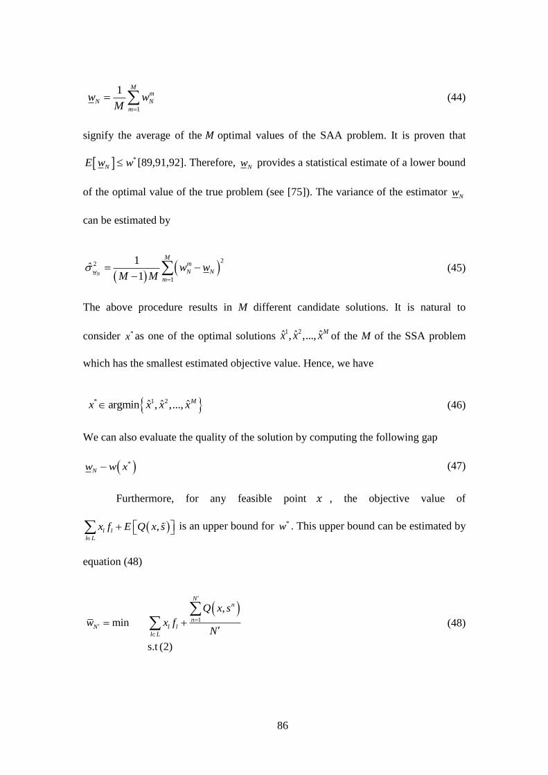
86
1
1 Mm
N N
m
w wM
(44)
signify the average of the optimal values of the SAA problem. It is proven that
*
NE w w [89,91,92]. Therefore, Nw provides a statistical estimate of a lower bound
of the optimal value of the true problem (see [75]). The variance of the estimator Nw
can be estimated by
2
2
1
1ˆ
1N
Mm
w N N
m
w wM M
(45)
The above procedure results in M different candidate solutions. It is natural to
consider *x as one of the optimal solutions 1 2ˆ ˆ ˆ, ,..., Mx x x of the M of the SSA problem
which has the smallest estimated objective value. Hence, we have
* 1 2ˆ ˆ ˆargmin , ,..., Mx x x x (46)
We can also evaluate the quality of the solution by computing the following gap
*
Nw w x (47)
Furthermore, for any feasible point , the objective value of
,l l
l L
x f E Q x s
is an upper bound for *w . This upper bound can be estimated by
equation (48)
1
,
min
s.t (2)
Nn
nN l l
l L
Q x s
w x fN
(48)

87
where N is the sample size of scenarios and it is chosen to be significantly
larger than N Given the above explanation, the SAA method applied in
this research is presented in the following.
We stated that increasing the number of facilities, and consequently the
number of scenarios significantly increase the computational time of the SCD-CVaR
model. Therefore, we apply the SAA method in addressing the large sized problems
for identifying a good lower bound to the original problem.
In this research the general SAA algorithm is implemented with some
modifications to fit the problem studied. We denote this algorithm as modified-SAA.
However, for the sake of comparison with the results of modified-SAA, we also
present the result of the general SAA algorithm in Section 4.4.4.2.1. The
modifications are summarized in the following.
First, in Section 4.4 we mentioned that the optimization problem, SCD-CVaR,
is modeled by using the AMPL mathematical programming language and solved with
Gurobi 4.5.6. We terminate Gurobi when the CPU time limit of 14,400 seconds is
reached. In this research, an estimate of the upper bound to equation (41), Nw , can be
derived by using the objective value of the solution to the SCD-CVaR which is
reported by Gurobi.
Second, in the general SAA algorithm a random scenario 1 2, ,..., NN s s s of
realizations of the random vector s is generated and an identical weight of 1
Nis
assigned to each single scenario (see [89]). In this research, we calculate the

88
probability of each scenario following the procedure presented in Section 3.4 where
the probability (weight) is equal s .
Figure 4-12 Scheme of modified-SAA algorithm for SCD-CVaR
4.4.4.2.1. Computational Result of modified-SAA Algorithm
To illustrate the applicability of the proposed modified-SAA method, a
numerical experiment is conducted in this section. The modified-SAA algorithm is
tested by using different combinations of sample sizes | | ∈ { , 1 , , } and
| | {1 , , , 1 }. The general SAA algorithm is tested by using the sample
size | | ∈ { , , ,1 , } and | | 1 .
The SAA algorithm presented in Figure 4-12 implemented and executed in
MATLAB 7.9 (2012) and tested on a single core of a Dell OptiPlex 980 computer
running the Windows 7 Enterprise 64 bit operating system with an Intel(R) Core(TM)
i7 CPU860@ 2.80GHz, and 8GB RAM.
modified-SAA.
1. Sample 𝑀 scenarios of size 𝑁 randomly from the scenario set 𝑆. Let 𝜔𝑀 be the set of
sampled scenarios.
2. Solve the SCD-CVaR problem with the reduced scenario set 𝜔𝑀 , and let be the
probability of occurrence for scenario 𝑠 in set 𝜔𝑀.
3. Repeat steps 2 𝑀 times.
4. Let and be the corresponding optimal objective values and
vectors of selected facilities, respectively.
5. Calculate the average of all the solutions (lower bound) and their variance for equation (28)
given equation (44) and equation (45). Compute the quality of estimated lower bound by
following (46) and using equation (47).
6. Compute the upper bound by solving equation (28) using Gurobi. Let the corresponding
objective value be given by where .
7. Compare lower bound and upper bound estimates by calculating the gap ( ). If
the bound gap is small enough, stop. Otherwise, increase 𝑁 and go to 1.

89
All of our computational experiments are based on the data that was generated
from the procedure presented in Section 3.4. We considered ten data instances for a
supply chain network consisting of ten facilities and ten consumers and we select 0.75
for the risk-level α. Table 4-7 reports the average of the optimal value/ best solution
found from Gurobi for each data instances. As per the results obtained, none of the ten
data instances resulted in an optimal solution within the prescribed time limit of
14400 seconds. We consider the average of ten data instances as the upper bound and
we consider 14210174 as Nw in our computation.
Table 4-7 Results obtained from AMPL for ten facilities and ten customers Data
Instance no.
best solution
found (upper bound)
1 16709100*
2 14934928*
3 12993917*
4 15981710*
5 13799333*
6 12847419*
7 14348449*
8 15010500*
9 11525948*
10 13950441*
Average 14210174
*: Best objective values found
Table 4-8 summarizes corresponding computational results of the modified-
SAA algorithm in detail. Note that the presented results are the average of ten data
instances. The first and second columns present the number of replications and the
sample size, respectively. The third column provides the estimated objective value of
the corresponding problem. The fourth and fifth columns represent the gap between
the best solution found by modified-SAA algorithm and the estimated objective value,

90
and the standard deviations of the estimator Nw , respectively. The CPU time, the
average optimality gap (average gap between the lower bound and the upper bound)
and finally the 95% confidence interval for the optimality gap display in the sixth,
seventh and eighth columns, correspondingly. It is clear from Table 4-8 that the
solution quality can be improved by increasing the sample size however, we observe
that average optimality gap remains above 0.50 even if we increase the sample size N.
That is because in the set of scenarios we have some scenarios with very small
probability values. Hence, these values result in small objective value. As a result, in
this research we also implemented the general SAA algorithm to compare the results
of these two algorithms. The results are presented in Table 4-9.
Table 4-8 Computational results of modified-SAA algorithm
| | | | Nw % *
Nw w x ˆNw Time (s)
% Avg.
optimality gap Avg. CI of LB at 95%
128 8 395388 0.93 36173 58 0.96 (390056, 400718)
64 16 795,204 0.83 48225 190 0.92 (794000, 796409)
32 32 2485926 0.71 121609 832 0.82 (2479102 , 2492750)
16 64 3309112 0.49 296420 1301 0.76 (3022096, 3340950)
The computational results in Table 4-9 indicate that the general SAA
algorithm leads to a considerably lower average optimality gap compared to the
modified-SAA algorithm. We also observe that, in the general SAA algorithm the
quality gap ( *
Nw w x ) and the computational time are notably smaller than the values
achieved in Table 4-8 for modified-SAA algorithm.
To summarize the results of this section, the general SAA leads to a better gap
for the SCD-CVaR model with a shorter computational time compared to the
modified-SAA algorithm. However, these solutions differed from the exact solutions
obtained by Gurobi for the first-stage decision variable. Based on our computational

91
experiences, the modified-SAA algorithm resulted in solutions that better matched the
first-stage decision variables from the exact solution in spite of the worse lower
bound. For larger instances however, the solution times exceeded 2 hours of
computations i.e., solution times are remarkably longer as problem size increases.
Table 4-9 Computational results of general SAA algorithm
| | | | Nw % *
Nw w x ˆNw Time (s)
% Avg.
optimality gap Avg. CI of LB at 95%
10 20 10002040 0.017 71056 1.9 0.30 (9943880 , 10060320)
10 30 10133810 0.016 66349 5.0 0.28 (10078770, 10187070)
10 50 10343740 0.016 60788 28.7 0.27 (10294310, 10393170)
10 100 10563830 0.015 67567 231.2 0.25 (10512490, 10615160)
10 300 10770100 0.011 54922 4794.6 0.22 (10727620, 10812690)
4.5. Conclusions and Future Research
In this chapter, we presented a supply network design problem with
application in the pharmaceutical industry to hedge against unreliability of capacity
and prevent shipping of tainted materials to the consumers. We studied a risk-neutral
decision-making policy and a risk-averse decision-making policy. We characterized
the trade-off between the risk and cost, which provides several insights on the impact
of risk-aversion on the facilities’ optimal decisions in a pharmaceutical supply chain.
Our studies demonstrated how strategic and tactical decisions change with respect to
the risk level. We found that an increase in the risk level leads to the selection of
not only more reliable facilities but also a different number of facilities. The risk-
averse policy also resulted in fewer worst-case scenarios as compared to the risk-
neutral policy. Our computations also revealed that becoming more risk-averse
resulted in remarkable increases in the cost of shipping untainted products to
consumers.

92
Our experience from solving the problem using AMPL-Gurobi indicated that
the number of facilities considerably increases the computational time. As a result, we
developed a metaheuristic approach to effectively solve the presented model. We
observed that the SA algorithm provides solutions within 5% of the solutions found
by Gurobi for both small-size and large-size problems. We also applied the SAA
algorithm to obtain a good lower bound for SCD-CVaR problem and also solutions to
the first-stage problem. We considered two approaches for our SAA algorithm. In the
first approach, we modified SAA algorithm in order to be able to use the set of
scenarios based on our procedure we developed in this research. For the second
approach, we considered the general SAA algorithm. Our results indicated that the
general SAA led to a lower average optimality gap with a shorter computational time
compared to the modified-SAA algorithm. However, based on our computational
experiences, the modified-SAA algorithm resulted in better solutions for the first-
stage decision variables. For larger instances however, the solution times exceeded 2
hours of computations, i.e., solution times are remarkably longer as problem size
increases. As a future extension, we wish to investigate some techniques such as
Bender Decomposition or L-shaped methods to efficiently solve the problems.
The significance of this chapter is two-fold. First of all, to the best of our
knowledge there is no currently available research to evaluate pharmaceutical (or
healthcare) supply chain network design with respect to sending tainted materials to
the consumer. Secondly, there is also little prior research to date that investigates
supply chain risk within the context of the pharmaceutical supply chain. As
pharmaceutical availability and drug safety clearly are key components to effective

93
patient quality of care, our models can assist supply chain designers enhance patient
safety and quality of patient care.
There are some interesting future research extensions. An extension of the
presented work is to include demand uncertainty and/or seasonal demand. Moreover,
we assumed an inspection and discard approach, which is not a valid assumption in
some supply chains like the automotive and electronics industries. This assumption
can be shifted to an inspection and fix (rework) approach where defective products
can be repaired after detection. Ultimately, we have considered instances that
included five facilities. However, experience from solving the models using
commercial software indicated that the number of facilities can dramatically increase
the computational time. We also think it is important to design and develop heuristic
techniques to obtain acceptable solutions to these larger size problems in reasonable
runtimes and with good solution quality.

94
CHAPTER FIVE
5. An Statistical Analysis of Facility Selection Process
5.1. Statistical Analyses Motivation
In this chapter, we will consider statistical analyses for the SCD and SCD-
CVaR models. In review of our computational analysis, we found that the selection of
some of facilities were obvious based on parameter values such as capacity or fixed
cost. In other cases, the facilities which appeared to be desirable were not selected.
Hence, it may be difficult to predict or determine which facilities are selected or
unselected; it may also be difficult to interpret the output of the SCD or SCD-CVaR
models. We perform a regression analysis in order to identify factors for predicting
the selection of a facility in the SCD and SCD-CVaR frameworks at various risk
levels and to analyze relationships among variables. The second purpose for
conducting a regression analysis in this context is to assess the probability of selection
for each individual facility at various risk levels ( ). We will also determine the
probability of selection for a set of selected facilities or alternatives.
Let us consider a supply chain network consisting of five facilities and five
consumers where the total demand of the consumers is 908 units. The values of the
parameters for this example are presented in Table 5-1.

95
Table 5-1 Values for an example of a supply chain network
Facility
#
Fixed cost ( ) Inspection
cost ( )
Fraction of
tainted items
before
inspection ( )
Fraction of
remained tainted
items after
inspection ( )
Reliability
(l )
Capacity
( )
Ratio
capacity/total
demand
1 1068072 90025 0.28 0.08 90% 136 15%
2 1764329 77067 0.25 0.07 52% 359 40%
3 1565588 53977 0.17 0.08 89% 317 35%
4 1358214 95728 0.26 0.03 73% 247 27%
5 1302468 61519 0.12 0.02 85% 176 19%
From Table 5-1, we observe the following relations
> > > > 1
> 1 > > > .
Figure 5-1 illustrates this tradeoff between l and
lq for various values of which is
the result of an optimal solution. For the SCD and 0.50
SCD-CVaR
models, we expect
either a smaller number of selected facilities or facilities with lower fixed cost. As we
observe in Figure 5-1, for SCD and 0.50SCD-CVaR , facility 1 and facility 5 are not
selected which are facilities with the lowest fixed cost, respectively. However, as we
observe in Table 5-1, facility 1 and facility 5 are the facilities with the highest and
lowest fraction of tainted products before inspection, respectively. Facility 1 and
Facility 5 also have the lowest capacity among all facilities. That indicates that in
SCD and 0.50SCD-CVaR model, the selection of facilities was a trade-off between
fixed cost or capacity and fraction of tainted products.

96
In 0.65SCD-CVaR , 0.75SCD-CVaR and 0.85SCD-CVaR , facility 4 is not selected
which is the most expensive facility for performing inspections. In 0.95SCD-CVaR and
0.99SCD-CVaR , decision making is based on a highly risk-averse policy and almost no
risk is acceptable. Therefore, the model mainly focuses on minimizing 5% and 1% of
the worst outcomes and shipping the least amount of tainted items to consumers,
respectively. However, it is unclear why Facility 5 (which is the facility with highest
fraction of untainted products before inspection) is not selected. Consequently,
another method should be considered to predict the selection of facilities based on
reliability or other factors. Moreover, when moving from a risk-neutral to a risk-
averse policy, fixed costs, capacity, or perhaps other factors may not be sufficient in
predicting which facilities will be selected or unselected. In the next section, a
regression analysis is conducted.

97
Figure 5-1 Tradeoff of capacity vs. fraction of tainted products (at various risk-levels)
5.2. Logistic Regression Analysis
The response variable, selecting a facility, is dichotomous or binary. A linear
regression model is inappropriate to predict a binary response variable for the
following reasons:
A linear regression analysis assumes a continuous response which is
unconstrained and can vary over the range of − to + whereas for
0.00 0.15 0.30
100
150
200
250
300
350
400
Fraction of Tainted
Capacity
0.00 0.15 0.30
100
150
200
250
300
350
400
Fraction of Tainted
Capacity
SCD
L2
L3
L4
L1
L5
0.00 0.15 0.30
100
150
200
250
300
350
400
Fraction of Tainted
Capacity
0.00 0.15 0.30
100
150
200
250
300
350
400
Fraction of Tainted
Capacity
Alpha = 0.5
L2
L3
L4
L1
L5
0.00 0.15 0.30
100
150
200
250
300
350
400
Fraction of Tainted
Capacity
0.00 0.15 0.30
100
150
200
250
300
350
400
Fraction of Tainted
Capacity
Alpha = 0.65
L1
L2
L3
L5
L4
0.00 0.15 0.30
100
150
200
250
300
350
400
Fraction of Tainted
Capacity
0.00 0.15 0.30
100
150
200
250
300
350
400
Fraction of Tainted
Capacity
Alpha = 0.75
L1
L2
L3
L5
L4
0.00 0.15 0.30
100
150
200
250
300
350
400
Fraction of Tainted
Capacity
0.00 0.15 0.30
100
150
200
250
300
350
400
Fraction of Tainted
Capacity
Alpha = 0.85
L1
L2
L3
L5
L4
0.00 0.15 0.30
100
150
200
250
300
350
400
Fraction of Tainted
Capacity
0.00 0.15 0.30
100
150
200
250
300
350
400
Fraction of Tainted
Capacity
Alpha = 0.95
L1
L2
L3
L4
L5
0.00 0.15 0.30
100
150
200
250
300
350
400
Fraction of Tainted
Capacity
0.00 0.15 0.30
100
150
200
250
300
350
400
Fraction of Tainted
Capacity
Alpha = 0.99
L1
L2
L3
L4
L5
Selected
Not Selected

98
dichotomous variables, the observed outcome is bounded and binary, with
only two as possible values.
The error terms produced from such a model will not be normally distributed.
A logistic regression models the relationship between a two-level categorical response
variable (binary response) and a set of explanatory (independent/predictor) variables
which can be quantitative or qualitative. Assume we have observed independent
variables 1, , …, on a group of subjects. We wish to use this information to
describe the probability that a facility will be selected given the values of the k
independent variables 1, , … , . For notational convenience, we denote the
probability statement 1 2( 1| , ,..., )KP y X X X as simply X . The status of a facility, , is
a binary response variable coded as 1y or 0y with respective probability
1 2( 1| , ,..., )l KX P y X X X and 1 21 1 ( 1| , ,..., ).l KX P y X X X The probability of
selecting a facility is described by following relationship
1 1 2 2
1 1 2 2
...
1 2 ...( 1| , ,..., ) .
1
k k
k k
o X X X
l K o X X XP y X X X e
e
(49)
The terms , 1, …, and in this model represent unknown parameters and must be
estimated based on data obtained on the values of the predictor and response variables
for a group of subjects. By rearranging equation (49) the odds of selecting a facility
can be expressed as:
1 1 2 2 ...
.1
k ko X X XX
Xe
(50)
Therefore,

99
1 1 2 2ln ... .1
k k
XY o X X X
X
(51)
This transformation , in equation (51), is called the logit transformation. This also
turns equation (49) into a linear regression model. Note that
ln
1
X
X
is the log
odds.
The odds are another way to express the likelihood that an event will occur.
The odds is a ratio of the probability that some event will occur over the probability
that it will not occur. For instance, if is the probability of selecting a facility
(e.g., 1y ), then 1 − which is the probability of that facility not being
selected. Therefore, the odds ⁄ which indicates that the likelihood that this
facility is selected is four times the likelihood of this facility is not being selected. The
advantage with using the odds is that, unlike a probability value, odds have no upper
bound. Therefore, a small change in a probability value results in large change in
odds. A value of one for odds indicates that the probability of selection and
probability of not selecting a facility are the same. Our interest is in the change of the
dependent variable for a one unit change in the independent variables, or the “Odds
Ratio (OR).” The OR is the ratio of the odds of the event for one value of one
independent variable (e.g., capacity) divided by the odds for a different value of that
independent variable (for instance, a value one unit lower for capacity when other
variables are constant in the model). Hence, the OR indicates the amount of change in
the odds and the direction of the relationship between an independent variable and
dependent variable.

100
In general, we can state that an OR of one indicates that the odds of selecting a
facility are the same; an OR greater than one indicates that the odds of selecting a
facility increases (a positive relationship); and an OR less than one indicates that the
odds of selecting a facility decreases (a negative relationship). Table 5-2 gives a
comparison of the standard linear regression model with the logistic regression model.
Table 5-2 Comparison of linear and logistic regression models Linear regression Logistic regression
Model + 1 1 + + 𝑡 + 1 1 + +
Response Continuous variable Binary variable
Covariates Continuous or discrete Continuous or discrete
Meaning of
coefficient
Amount of expected
change in the response y
per unit change in covariates
Amount of change of log
odds per unit change in the covariates
Let ˆl and denote the fitted value for facility and the corresponding estimated
coefficients, respectively. We can rewrite the estimated odds equation as:
(1− ) + + + +
or,
1 1 2 2
ˆˆ ˆ ˆ ˆˆ ln ... .
ˆ1k k
XY o X X X
X
(52)
Thus, given the above equation for each one unit increase in while keeping other
predictors constant, the predicted odds is increased by a factor of ( ). In other
words, ( ) is an odds ratio, which denotes the odds at + 1 divided by the
odds . Similarly, if all predictors are set equal to 0, the predicted odds is ( ).

101
We will also consider the interaction between the variables. If two
independent variables interact, then the effect of one of them on the dependent
variable varies depending on the value of the other independent variable. The
presence of interactions can have important effects for the interpretation of regression
model. Interaction is assessed by adding the cross-product term (e.g., 1 ) to the
model. For instance, by assuming an interaction between −1 and we can rewrite
equation (52) as following:
1 1 2 2 1 1
ˆˆ ˆ ˆ ˆ ˆˆ ln ... .
ˆ1k k k k k
XY o X X X X X
X
(53)
Now, for each one unit increase in , the increase in the predicted odds is a factor of
( + +1 −1). That is, an independent variable whose effect on the dependent
variable is considered to vary as a function of the −1. Note that an increase in the
logit is in favor of the probability of selecting a facility since by increasing
1− ,
would also increase.
5.2.1. Description of the Data Source
In this section, we define a set of continuous predictor variables that are
hypothesized to be associated with the dependent variable, which is the status of a
facility being selected or unselected. The predictors for facility l include the
following: the reliability of the facility ( l ), the fixed cost of opening the facility ( lf
), the capacity of the facility ( l ), the fixed cost of implementing an inspection at the
facility ( ln ), the total demand of the consumers (c
c C
b b
), the fraction of tainted

102
products at the facility l ( lsq ); the fraction of tainted products at facility l after
inspection (lsr ); and risk level ( ). We will investigate the impact of these factors on
the status of a facility. The status of a facility is represented by an indicator variable
defined as follows:
1, if facility is selected,
0, else .l
l l Ly
We use 50 data files for a specific case containing five facilities and five
consumers. We consider seven levels for : 0, 0.50, 0.65, 0.75, 0.85, 0.95 and 0.99.
Therefore, in total we will have 1750 (50*5*7) observations. To ensure that the data
generated are uniformly spread out over the defined ranges (defined in 3.4); we
consider the histogram for each single factor in Figure 5-2.
Figure 5-2 Histogram of each variable
Given the histograms in Figure 5-2, we observe that data is distributed nearly
uniformly over the variable ranges. We also consider a similar histogram for each

103
single facility to verify that each individual facility also has data over the predefined
ranges. As an example, histograms for facility 1 are presented in Figure 5-3.
Figure 5-3 Histogram of the data for Facility 1
Strong linear relationships among predictor variables might imply
multicollinearity and cause imprecise regression coefficients that are difficult to
interpret. The relationship between two quantitative variables may be displayed
graphically by means of a scatterplot. The scatter plots between pairs of predictor
variables are illustrated in Figure 5-4.

104
Figure 5-4 Scatter plot of the selected variables
A positive linear relationship between the two quantitative predictor variables
is indicated on a scatterplot by an upward linear trend whereas a negative linear
relationship is indicated by the opposite effect. Otherwise, if the points do not show a
linear trend, multicollinearity should not be an issue. When we inspect the plots in
Figure 5-4, it becomes apparent that a positive association between capacity and fixed
cost (correlation = 0.70) and and inspection cost (correlation =0.73) exist. This
association may be due to the assumption that we considered during generating the
data. One way to overcome this issue is to exclude one of the variables from the
model. Combining two or multiple variables into a single variable may be another
alternative. Hence, we exclude fixed cost ( ) and we define a function for the
relationship between capacity and total demand of consumers (∑ ∈ ) which is

105
define as ,1
ll
c
c C
b
. This ratio implies the fraction of the total demand that can be
covered by a facility. In addition, we exclude inspection cost and consider
,2 1l l lq r . This fraction indicates the maximum percent of untainted products
that we can expect from facility l after performing an inspection. Therefore, we
consider risk-level ( ), reliability of facility l ( l ), the fraction of the total demand
that can be covered by facility l (,1l ), and the maximum percent of untainted
products that we can expect from facility l after performing an inspection (,2l ) as our
independent variables in the statistical analyses. In the next section, we discuss our
regression model.
5.2.2. Model Description
The main analysis of this section uses a logistic regression model to consider
the relationship of the independent variables with the dependent variable. The first
order logistic regression model is presented as follows:
0 1 2 3 ,1 4 ,2
0 1 2 3 ,1 4 ,2,1 ,2( 1| , , , )
1
l l l
l l ll l l lP y e
e
(54)
and given (51)
0 1 2 3 ,1 4 ,2ln .l l l lY odds (55)
And given the equation (55), the mean response function for the log odds is written as
0 1 2 3 1 4 2.lE Y (56)
The regression model with interaction is as follows:

106
0 1 2 3 ,1 4 ,2 5 6 ,1 7 ,2
8 ,1 9 ,2 10 ,1 ,2 .
l l l l l l l
l l l l l l
Y
(57)
The mean response function for equation (57) can be written as follows:
0 1 2 3 1 4 2 5 6 1 7 2
8 1 9 2 10 1 2.
lE Y
(58)
We consider two approaches for our statistical analysis. In the first approach,
as we assumed in Section 3.4, we assume the cost of selecting a facility is correlated
with the capacity such that the facility with the highest capacity has the highest fixed
cost of selection. In the second approach, however, we assume that cost of selecting a
facility is correlated with the reliability of a facility or the probability of facility being
in state 0 ( l ). The statistical analysis in this research was executed in the software
package R (64-bit) version 2.11.1.
5.2.2.1. Approach 1
The coefficients from the estimated regression model for the first approach,
when we assume the cost of selecting a facility is correlated with the capacity are
given in Table 5-3. In Table 5-3, the coefficients, their standard errors, Wald test
statistic, and the associated p-values are given. In logistic regression, the significance
of a predictor variable is assessed via the likelihood ratio Chi-square test or Wald test
[86]. At any step in the procedure, the variable with the smallest p-value is the one
that produces the greatest change in the log-likelihood relative to a model not
containing the variable. The Wald test statistic is computed by dividing the estimated
coefficient of interest by its standard error (𝑆 ( ) 𝑎 ( )1
⁄ where is the
estimated coefficient). For instance, from Table 5-3 we observe that the regression

107
coefficient for is significant at 0.05 level and 1 is significant at 0.01 level whereas
2 is not significant in this approach. Table 5-3 also indicates that interaction between
and 1 , and the interaction between 1 and 2 are highly significant at 0.001 level.
Given Table 5-3, we have
1 2 1
2 1 2 1 2
ˆ ln 5.53 8.41 6.10 60.20 11.81 1.53 20.22
2.46 6.77 5.15 99.26
lY odds
(59)
Table 5-3 Logistic regression model result for approach 1
Research Model
Predictors
Logistic
Coefficients Std. Error
z value
(significance level) Pr(>|z|)
(Intercept) 5.35 8.06 0.66 0.51
-8.41 4.01 -2.09* 0.03
6.10 9.09 0.67 0.50
1 -60.41 19.23 -3.14** 0.00
-11.81 9.97 -1.19 0.24
1.53 2.36 0.65 0.52
1 20.22 4.10 4.93*** 0.00
2.46 4.40 0.56 0.58
1 -6.77 14.18 -0.48 0.63
-5.15 9.77 -0.53 0.60
1 99.26 27.81 3.57*** 0.00
Significant codes: ‘***’ < 1; ‘**’ < 1; ‘*’ < 5; ‘.’ < 1; ‘’ 1, AIC = 925.0
5.2.2.1.1. Approach 1 Interpretation
As stated, when a model has interaction between variables, it attempts to
describe how the outcome for an independent variable is different depending on the
level of another independent variable. We present an example of how to interpret the
fitted model here to clarify the interaction interpretation in our regression model.
From Equation (59), it can be shown that the change in the logit (or log odds) with
0.25 unit increase in when other variables are held constant is

108
0.25
, 1 2ˆ ˆ ˆ 2.01 0.38 5.05 0.61 .l l lY Y Y
(60)
Equation (60) indicates that when a model has interaction term(s) of two independent
variables, the effect of one independent variable on the dependent variable varies
depending on the value of the other independent variable. Let’s assume the reliability
of a facility is 50 percent ( ), the facility can cover 15 percent of the demand
or 1 0.15 and we expect a maximum of 70 percent untainted products from facility
(i.e., 2 0.70 ) when 0.50 . From equation (60) we observe that increasing to
0.75 will result in changing the odds of the selecting the facility by approximately a
factor of 0.53. On the other hand, by considering a higher value for 2 , say 0.75
(which means reducing the fraction of expected tainted product), and keeping 1 at
the same level, we will observe approximately 3 percent increase in odds of selecting
the facility. By holding 2 at 0.70 and increasing 1 to 0.16, a 5% increase is
observed which indicates an increase in the likelihood of selecting larger facilities for
higher values of confidence level.
5.2.2.2. Approach 2
The coefficients from the estimated regression model for approach 2 are given in
Table 5-4. From Table 5-4 we observe that, the regression coefficient for is highly
significant at 0.001 level while in approach 1 this value is significant at 0.05 level.
Furthermore, 2 is significant at 0.01 level whereas this ratio itself was not significant
in approach 1. From Table 5-4 we also observe that unlike approach 1, and are
significant at 0.05 and 0.01 level, respectively. Interaction between and 2 is
significant at 0.1 level. Given Table 5-4,

109
1 2 1
2 1 2 1 2
ˆ ln 48.73 20.12 28.39 77.950 50.62 8.96 12.03
12.24 14.52 15.32 111.15 .
lY odds
(61)
Table 5-4 Logistic regression model result for approach 2
Research Model
Predictors
Logistic
Coefficients Std. Error
z value
(significance
level)
Pr(>|z|)
(Intercept) 48.73 12.38 3.94*** 0.00008
-20.12 5.25 -3.84*** 0.00013
-28.39 14.30 -1.99* 0.04704
1 -77.95 42.70 -1.83. 0.06790
-50.62 17.85 -2.84** 0.00458
8.96 3.14 2.86** 0.00430
1 12.03 8.53 1.41 0.15843
12.24 6.85 1.79. 0.07384
1 14.52 27.23 0.53 0.59370
15.32 13.62 1.13 0.26045
1 111.15 63.26 1.76. 0.07890
Significant codes: ‘***’ < 1; ‘**’ < 1; ‘*’ < 5; ‘.’ < 1; ‘’ 1, AIC = 999.15
5.2.2.2.1. Approach 2 Interpretation
From equation (61), the change in the log odds with 0.25 unit increase in
when other variables are held constant is
0.25
, 1 2ˆ ˆ ˆ 5.03 2.24 3.01 3.06 .l l lY Y Y
(62)
Given , 1 0.15 and 2 0.70 , the change in the odds of the selecting the
facility will be a factor of 0.26. If we increase to the increase in odds of
the selecting the facility of will be 0.23 percent which indicates increasing the
reliability of a facility will result in increasing the likelihood of selecting the facility.

110
5.2.3. Stepwise Regression
From Table 5-3 and Table 5-4, it is observable that not all coefficients are
significant. For instance, the coefficient for the interaction between and 2 is not a
significant predictor in approach 1. We therefore apply a stepwise selection procedure
to obtain only the variables are significant predictors for status. The stepwise logistic
regression (SLR) method allows the model to be assessed as it is being built. In the
SLR, predictor variables are selected for inclusion or exclusion from the regression
model based on a stepwise selected method.
Stepwise regression method is a combination of the forward selection and
backward elimination, testing at each iteration for variables to be included or
excluded. Forward selection starts with no variables and selects variables if they are
statistically significant. Backward elimination starts with all candidate variables,
examining them one by one for statistical significance, and finally, eliminating the
ones that are not significant. The R software package has an option that allows the
user to perform the stepwise procedure.
The Akaike Information Criterion (AIC) approach is used to obtain the log-
likelihood value. At any step in the procedure, a statistically significant variable is the
one that produces the greatest change in the log-likelihood relative to a model not
containing the variable [93]. The AIC is based on a likelihood theory and is a function
of the number of observations , the sum of squared errors SSE and the number of
parameters estimated in the model , as shown in the following:

111
AIC ln 2SSE
n pn
.
The first term in the above equation is a measure of the model lack of fit while the
second term is a penalty term for additional parameters in the model. Therefore, as the
number of parameters included in the model increases, the lack of fit term should
decrease due to the decrease of the error while the penalty term increases. On the
other hand, as variables are dropped from the model, the lack of fit term should
increase while the penalty term decreases. The model with the smallest AIC is
considered the best model since it minimizes the difference from the given model to
the true model. The AIC after implementing the stepwise selection method for
approach 1 is 918.9 while the calculated AIC for equation (59) was 925.0. Therefore,
we select the model resulting from the combination model. The coefficients from the
estimated regression model for approach 1 after performing the stepwise selection
method are given in Table 5-5.
Table 5-5 Logistic regression model result for approach 1 after performing SLR
Research Model
Predictors
Logistic
Coefficients Std. Error
z value
(significance level) Pr(>|z|)
(Intercept) 5.81 3.48 1.67. 0.10
-2.59 0.79 -3.25** 0.00
1.57 0.75 2.09* 0.04
1 -55.99 18.08 -3.10** 0.00
-12.30 4.23 -2.91** 0.00
1 19.02 3.99 4.76*** 0.00
1 88.79 22.22 4.00*** 0.00
Significant codes: ‘***’ < 1; ‘**’ < 1; ‘*’ < 5; ‘.’ < 1; ‘’ 1, AIC = 918.87
From Table 5-5, performing a stepwise procedure resulted in excluding a few of the
interactions and reducing the AIC by almost seven units to 918.9. Given Table 5-5, let
us rewrite equation (59) as follows:

112
1 2 1 1 2ˆ 5.81 2.59 1.57 55.99 12.30 19.02 88.796 .lY
(63)
In the logistic regression model (63), some of the interaction term still exists. From
equation (63), the coefficient for is -2.59 and by increasing by 0.25 unit, the odds
ratio will be − + . For instance, when 1 is held at 0.15, we will have 0.06
for the odds increase and the odds for 1 equal 0.16 will 0.31 which indicates more
than 60 percent increase in odds of selecting the facility.
The coefficients from the estimated regression model for approach 2 after
performing the stepwise method are given in Table 5-6. From Table 5-6 we observe
that performing a stepwise procedure resulted in excluding a few of the interactions
and reducing the AIC by nearly 3 units to 996. Given Table 5-6, the regression model
for approach 2 with interaction is as follows:
1 2 2 1 2ˆ 44.61 17.45 12.39 85.80 47.12 10.04 142.16 12.39 .lY
(64)
Table 5-6 Logistic regression model result for approach 2 after performing SLR
Research Model
Predictors Logistic Coefficients Std. Error
z value
(significance level) Pr(>|z|)
(Intercept) 41.66 9.25 4.50*** 0.0000
-17.45 4.99 -3.49*** 0.0005
-12.39 2.35 -5.28*** 0.0000
1 -85.80 32.92 -2.61** 0.0092
-47.12 11.39 -4.14*** 0.0000
10.04 3.06 3.29** 0.0010
142.16 39.44 3.61. 0.0003
1 -12.39 2.35 -5.28*** 0.0000
Significant codes: ‘***’ < 1; ‘**’ < 1; ‘*’ < 5; ‘.’ < 1; ‘’ 1, AIC = 996.62

113
5.2.4. Prediction
To evaluate the predictive ability of the model based on the estimated logistic
coefficients in Table 5-5 and Table 5-6, we perform prediction for both approach 1
and approach 2 for a set of 5 facilities. We consider two risk-level values for all the
facilities, i.e., , . The data and the result of prediction are presented in
Table 5-7 and Table 5-8. Note that in approach 1 facilities are sorted based on their
capacity and in approach 2 facilities are sorted based on their reliability.
The results in Table 5-7 indicate that 1 is a very significant attribute when
selecting a supplier in approach 1. For instance, the likelihood of selecting the facility
with the highest capacity (i.e., Facility 1) is 0.607 for =0.50 whereas this facility has
the worst reliability among the others and only 71 percent of its capacity can be used
after inspection. We also observe 9% growth in likelihood of selection for Facility 1
for =0.95. As another example, Facility 4 is the most reliable facility and provides a
large portion of untainted products even after inspection. However, we observe a
small likelihood of selection since its capacity is small. The likelihood of selection
reduces even more when increases to 0.95.
Table 5-7 Likelihood of selection of facilities in approach 1
Facility
# reliability 1
=0.50
=0.95
Probability
of selection logit
Probability
of
selection
logit
2 0.7457 0.2782 0.7587 0.780 1.265
0.829 1.581
4 0.9084 0.1264 0.8992 0.425 -0.304
0.397 -0.420
3 0.8392 0.1916 0.9074 0.711 0.901
0.725 0.971
5 0.8326 0.1068 0.8324 0.276 -0.965
0.243 -1.136
1 0.5024 0.3006 0.7146 0.607 0.435
0.693 0.815

114
A notable observation from Table 5-7 is that, for higher risk-level the likelihood of
selecting a facility decreases for facilities with smaller capacities. This indicates that
in approach 1, a risk-averse decision-maker tends to provide more capacity to hedge
against risk.
The results in Table 5-8, however, indicate that higher weight assigned to
reliability of a facility in approach 2 as compared to approach 1. A notable
observation from Table 5-8 is that Facility 5 has the lowest reliability but its capacity
is the largest. The probability of selecting facility 5 for =0.50 is 0.995. However,
after increasing risk-level to 0.95, the probability of selecting facility 5 decreases
to 0.965. This decrease indicates that more reliable facilities are selected in risk-
averse decision making policy. These results can be useful for facilities as well since
it enables them to analyze their situation and compare it with other facilities
(competitors) and attempt to change their behaviors in order to increase their
likelihood of selection. We believe that other important implications in practice can
be achieved through this result.
Table 5-8 Likelihood of selection of facilities in approach 2
Facility # reliability 1
=0.50
=0.95
Probability
of selection logit
Probability
of
selection
logit
3 0.6027 0.1098 0.8443 0.006 -5.141
0.005 -5.279
4 0.5624 0.2045 0.7535 0.408 -0.371
0.341 -0.643
1 0.8701 0.1277 0.8068 0.044 -3.068
0.102 -2.725
2 0.8385 0.2915 0.7989 0.809 1.895
0.866 2.053
5 0.5563 0.3501 0.7167 0.995 5.254
0.965 3.915
5.2.5. Key Observations
Recall that in approach 1 we assumed that the cost of selecting a facility is
correlated with the capacity such that the facility with the highest capacity has the

115
highest fixed cost of selection. In approach 2, however, we assume that cost of
selecting a facility is correlated with the reliability of a facility or the probability of
facility being in state 0. We summarize our observations from approach 1 and
approach 2 and also risk-neutral and risk-averse decision making policies as
following:
Facilities with larger capacities have higher likelihood of selection when
capacity drives facility cost.
When capacity drives facility cost, for higher value of (risk-averse policy)
the likelihood of selection goes down if capacity of facility goes down.
When reliability drives facility cost, increasing the reliability of a facility will
result in increasing the likelihood of selecting the facility.
When reliability drives facility cost, for higher value of risk-level the
likelihood of selection goes down if reliability and/or the fraction untainted
products that we can expect from facility l after performing an inspection go
down.
Provided that the problem is capacitated (i.e., the capacity is limited), “size” of
the facility is perceived to be the most important factor for facility selection in
the risk-neutral and risk-averse policies and also when capacity drives facility
cost and when reliability drives facility cost.
Under the risk-neutral policy, “reliability” of the facility is perceived to be the
least important factor.

116
5.3. Multinomial Logistic Regression (MLR)
In Section 5.2, we conducted a logistic regression analysis to assess the
likelihood of selection for each individual facility at various risk levels. In this
section, we assess the likelihood of selection for a set of selected facilities at various
risk levels. For instance, we assess the likelihood of selecting all the facilities together
or selecting all the facilities except Facility 1.
Suppose the set of selected facilities, , is a categorical response variable with
J categories. Let 1 2, ,..., J be the response probabilities satisfying 1JJ .
When one takes n independent observations, the probability distribution for the
number of outcomes that occur within each of the J types is a multinomial distribution
[94]. One value (typically the first, the last, or the value with the highest frequency) of
the dependent variable is designated as the reference or baseline category. The
probability of the other categories is compared to the probability of the reference
category. For instance, if there are four categories (alternatives), A, B, C, and D, and
the reference category is A, MLR will calculate the log odds (or estimates the set of
coefficients) for being in category B versus A, category C versus A, and category D
versus A. Each set of coefficients then represents the effect of a unit change in the
independent variables on the log odds of each category relative to the reference
category.
For a dependent variable Y with J categories, we require the calculation of J-1
log odds, one for each category relative to the reference category, to describe the
relationship between the dependent variable and the independent variables. As a

117
result, if the last category is the reference, then, for j = 1,…, J-1, the odds ratio of
category j with predictor x is
log , 1,..., 1.j
j j
J
x j J
(65)
The choice probability for the reference category J is
1
1
1.
1 j j j
J Jx
j
e
(66)
The response probabilities for 1,..., 1j J can be expressed as
1
1
.
1
j j
j j j
x
j Jx
j
e
e
(67)
5.3.1. Description of the Data Source
We consider risk-level ( ), the fraction of the total demand that can be
covered by facility l (,1l ) and the maximum percent of untainted products that we
can expect from facility l after performing inspection (,2l ) as our independent
variables. In the next section, we discuss our regression model. We use 120 data
instances for a specific case containing five facilities and five consumers. Hence, we
have 2 1L possible sets of alternatives of selected facilities as illustrated within
Table (c) in Appendix C. For instance, in Table (c) alternative “ee” indicates the
alternative that all facilities are not selected except Facility 1 and alternative “a” is the
alternative that all facilities are selected. We consider seven levels for the risk level :
0, 0.50, 0.65, 0.75, 0.85, 0.95 and 0.99. As a result, in total we will have 840 (120*7)

118
observations. Finally, for the sake of interpretability, we sort the reliability and
consequently ,2l in a descending manner so that Facility 1 is the most reliable facility
and Facility 5 is the least reliable facility. Moreover, as mentioned, strong linear
relationships among predictor variables might imply multicollinearity and cause
imprecise regression coefficients that are difficult to interpret. The relationship
between the independent variables is illustrated in Figure 5-5. By inspecting Figure
5-5, it becomes apparent that a positive linear association between some of the
independent variables exists. For instance, a positive linear association between 3,2
and 4,2 (correlation = 0.74),
1,2 and
2,2 (correlation = 0.62), and 1,1
and
3,1
(correlation = -0.43) exists. To overcome this issue, we convert ,2l from a
quantitative variable to a qualitative variable with three levels e.g., ‘‘1 = High
expectation” where ,2 0.86,0.94 ,l ‘‘2 = Medium expectation” where
,2 0.78,0.86l , and finally, ‘‘3 = Low expectation” where ,2 0.70,0.78l . We
also exclude 3,1 from the model.

119
Figure 5-5 Scatter plot of the selected MLR variables
5.3.2. Model Description
In our MLR model, the two-way interaction effects of the independent
variables are also considered. As an example, the coefficients from the estimated
results of multinomial logistic regression model ( 0.75 ) are given in Table 5-9.
Note that in Table 5-9, alternative “b” (which is the alternative that all facilities are
selected except the most reliable, i.e., Facility 1) is the reference category and the
probability of categories is compared to the probability of the reference category.
Hence, given Table 5-9 and equation (65) the log odds of the estimated MLR model
for alternative “c” (the alternative that all facilities are selected except the most
reliable i.e., Facility 2) is
1,1 2,1 4,1 5,1 1,2 2,2
3,2 5,2
log -39.917 33.024 -52.932 -33.941 -30.185 -2.9763 -0.39135
0.77611 +22.184 .
c
b
(68)

120
Table 5-9 Multinomial regression model result for
Research Model Predictors Multinomial Coefficients Std. Error t-value (significance level) Pr(>|t|)
altc -39.917 91761 -0.0004 1.000
alte -108.37 97011 -0.0011 0.999
alti 12.194 13.27 0.9189 0.358
altk 112.24 68579 0.0016 0.999
altq 12.708 12.075 1.0525 0.293
alty -29.662 93273 -0.0003 1.000
altc:ratio1.1 33.024 18.848 1.7521 0.080.
alte:ratio1.1 83.312 21.476 3.8793 0.000***
alti:ratio1.1 41.676 18.887 2.2065 0.027*
altk:ratio1.1 196.82 41190 0.0048 0.996
altq:ratio1.1 38.122 18.188 2.096 0.036*
alty:ratio1.1 248.92 158690 0.0016 0.999
altc:ratio1.2 -52.932 19.467 -2.719 0.007***
alte:ratio1.2 40.735 18.386 2.2156 0.027*
alti:ratio1.2 -9.789 16.319 -0.5999 0.549
altk:ratio1.2 -496.77 129650 -0.0038 0.997
altq:ratio1.2 0.72686 15.197 0.0478 0.962
alty:ratio1.2 160.25 91802 0.0017 0.999
altc:ratio1.4 -33.941 18.119 -1.8732 0.061.
alte:ratio1.4 18.031 19.3 0.9343 0.350
alti:ratio1.4 -32.748 17.018 -1.9243 0.054.
altk:ratio1.4 -344.04 76278 -0.0045 0.996
altq:ratio1.4 -37.84 16.147 -2.3435 0.019*
alty:ratio1.4 -221.36 76698 -0.0029 0.998
altc:ratio1.5 -30.185 18.861 -1.6004 0.110
alte:ratio1.5 35.907 22.438 1.6003 0.110
alti:ratio1.5 -17.671 18.982 -0.9309 0.352
altk:ratio1.5 -311.28 85893 -0.0036 0.997
altq:ratio1.5 -39.092 18.02 -2.1694 0.030*
alty:ratio1.5 -263.6 140030 -0.0019 0.998
altc:ratio2.1 -2.9763 2.7625 -1.0774 0.281
alte:ratio2.1 -1.7366 2.2707 -0.7648 0.444
alti:ratio2.1 -2.7198 2.1427 -1.2694 0.204
altk:ratio2.1 29.213 25202 0.0012 0.999
altq:ratio2.1 -2.7911 2.0057 -1.3916 0.164
alty:ratio2.1 14.456 27381 0.0005 1.000
altc:ratio2.2 -0.39135 1.9627 -0.1994 0.842
alte:ratio2.2 -0.83265 1.657 -0.5025 0.615
alti:ratio2.2 -0.38954 1.5294 -0.2547 0.799
altk:ratio2.2 44.571 14191 0.0031 0.997
altq:ratio2.2 -1.5184 1.4893 -1.0195 0.308
alty:ratio2.2 27.466 11428 0.0024 0.998
altc:ratio2.3 0.77611 2.1987 0.353 0.724
alte:ratio2.3 -0.8342 1.9577 -0.4261 0.670
alti:ratio2.3 -1.5974 1.9132 -0.8349 0.404
altk:ratio2.3 -33.976 17309 -0.002 0.998
altq:ratio2.3 -0.80602 1.8586 -0.4337 0.665
alty:ratio2.3 -8.3163 13081 -0.0006 0.999
altc:ratio2.5 22.184 30587 0.0007 0.999
alte:ratio2.5 22.296 32337 0.0007 0.999
alti:ratio2.5 1.1626 2.0254 0.574 0.566
altk:ratio2.5 13.27 15474 0.0009 0.999
altq:ratio2.5 3.2877 2.01 1.6357 0.102
alty:ratio2.5 -13.914 24695 -0.0006 1.000
Significant codes: ‘***’ < 1; ‘**’ < 1; ‘*’ < 5; ‘.’ < 1; ‘’ 1
Log-Likelihood: -77.582
McFadden R^2: 0.53146
Likelihood ratio test : chisq = 176 (p.value=< 2.22e-16)

121
5.3.3. Prediction
This section is concerned with the predictive ability of our resultant MLR
model. The data and the result of prediction are presented in Table 5-10 and Table
5-11, respectively. Note that we use identical data for all values of risk-level .
Table 5-10 Data used in prediction
1,1 0.250
2,1 0.223
4,1 0.278
5,1 0.258
1,2 1
2,2 2
3,2 3
5,2 3
The results of prediction are summarized in Table 5-11 (and illustrated in
Figure (e)). Several observations can be made from this table. For instance, we
observe how the probability of alternative “a” increases with increases to . This
observation confirms our results in Chapter 4 where we observed that for higher
values of risk-level, the number of selected facilities gradually increases. This
increase can be justified because a risk-averse decision-maker provides more capacity
(by selection of more facilities) in order to be able both to perform more inspections
and to discard more tainted products and still satisfy the total demand. Furthermore,
for 0.05 , there exists a (small) likelihood of selecting alternatives with a lower
number of selected facilities (i.e., the alternatives “u” and “y”).
Another result that we obtained in Chapter 4 was that, for higher values of ,
a risk-averse decision-maker tends to select more reliable facilities and vice versa. For
instance, alternative “b” is the alternative where the most reliable facility (Facility 1)
is not selected. From Table 5-11, we observe that increasing leads to a lower

122
likelihood of selecting this alternative which indicates that the tendency to close the
most reliable facility decreases with respect to increasing the risk-level . Moreover,
Facility 5 and Facility 4 are the least reliable facility and we observe the probability of
the alternatives “i” and “q” is larger when becoming more risk-averse. The result of
MLR verified the result of our computational analysis in Chapter 4 where we showed
that the risk-averse policy results in different strategic compared to the risk-neutral
policy.
Table 5-11 Prediction performance of MLR model
Alternatives
alpha Reference (baseline)
category
a b c e i q u y
11111 01111 10111 11011 11101 11110 11010 11100
0.05 b 0 0.272 0.270 0.013 0.090 0.339 0.005 0.011
0.5 b 0 0.222 0.315 0.022 0.096 0.343 0.000 0.002
0.65 b 0 0.038 0.481 0.002 0.076 0.403 0.000 0.000
0.75 b 0 0.008 0.690 0.000 0.058 0.244 0.000 0.000
0.85 a 0.0001 0.001 0.551 0.002 0.070 0.376 0.000 0.000
0.95 a 0.245 0.000 0.172 0.000 0.043 0.540 0.000 0.000
0.99 a 0.434 0.000 0.048 0.000 0.074 0.444 0.000 0.000
5.3.4. Conclusion
In conclusion, this chapter firstly identified the factors for predicting the
selection of a facility in the SCD and SCD-CVaR frameworks at various risk levels
and to analyze relationships among variables. Secondly, by conducting a logistic
regression analysis and multinomial regression analysis we assessed the probability of
selection for each individual facility at various risk levels along with probability of
selection for a set of selected facilities or alternatives.
The obtained results enable managers to identify the criteria that impact our
strategic decisions in both the risk-neutral and risk-averse decision-making policies.

123
The results also enable the facilities to analyze their situations and compare them with
other facilities (competitors) and to change their behaviors in order to increase their
likelihood of selection.

124
CHAPTER SIX
6. Conclusions and Future Research
6.1. Research Conclusions
In response to certain catastrophic events, particularly in the healthcare and
pharmaceutical supply chains, this research focused on risks that impact strategic and
tactical decisions in these types of supply chains. In contrast with most prior research,
in this dissertation we focused on the supply (capacity) management required to hedge
against the unreliability of capacity and to prevent the shipping of tainted materials to
the consumers.
We discussed models for designing supply chain networks resilient to capacity
disruptions. The goal was to design a supply chain infrastructure under the risk of
disruption, so that it operates with the highest possible efficiency (i.e., at low cost)
both normally and when a disruption occurs. However, such network design problems
belong to the class of NP-hard problems. Accordingly, heuristic algorithms and
metaheuristic approaches were developed to obtain the solutions to these types of
problems.
In Chapter 3, we considered a single-period, single-product supply chain with
capacitated facilities. We considered a risk-neutral decision-making policy based on a
cost-minimization approach and utilized a mixed integer stochastic programming
model formulated as a two-stage optimization problem. The goal of the model
consisted of the facility selection in the first stage, defining capacity (product)
allocation among the consumers, and inspection decisions. The objective was to
minimize the expected cost composed of the fixed cost of selecting the facility, the

125
cost of shipping untainted products, the cost of shipping tainted products, the cost of
inspection the facility, and the cost of discarding tainted products.
From solving the problem in AMPL, we observed that the number of facilities,
and consequently the number of scenarios, had a significant impact on the
computational time of our problem. Therefore, we developed nine constructive
heuristic methods, two improvement heuristic methods, and a Simulated Annealing
(SA) approach to solve the presented model effectively. Based on our computational
studies and statistical analyses, the SA approach is not efficient in terms of solution
quality and solution time for small-sized problems or a small number of scenarios.
However, some developed heuristics achieved good solution qualities in a more
reasonable time compared with the optimal or best found solution. Moreover, our
improvement heuristic algorithms were able to improve the solutions obtained from
constructive heuristics. Therefore, constructive and improvement heuristics were
preferable in small sized problems. However, for problems with ten or more facilities,
the SA approach outperformed constructive and improvement heuristics even though
it required higher computational time.
In Chapter 4, we addressed a risk-averse decision-making policy wherein
rather than selecting facilities and identifying the pertinent supplier-consumer
assignments that minimize the expected cost, the decision-maker uses a CVaR
approach to measure and quantify risk and to define what comprises a worst-case
scenario.
We characterized the trade-off between the risk and the cost and this provided
several insights on the impact of risk-aversion on the optimal decisions. Our studies
demonstrated how strategic and tactical decisions changed with respect to the risk

126
level. We found that an increase in the risk level leads to the selection of more
reliable facilities and a different number of facilities. The risk-averse policy also
resulted in fewer worst-case scenarios compared with the risk-neutral policy. Our
computations also revealed that becoming more risk-averse resulted in remarkable
increases in the cost of shipping untainted products to consumers.
Lastly, we considered statistical analyses for the risk-neutral and risk-averse
decision-making policies in Chapter 5. We found that the selection of certain facilities
was obvious based on parameter values, such as capacity or fixed cost. In other cases,
facilities that appeared to be desirable were not selected. Hence, it may be difficult to
predict or determine which facilities are selected or unselected; it may also be difficult
to interpret the output of the SCD or SCD-CVaR models. Hence, we conducted a
regression analysis to identify factors for predicting the selection of a facility at
various risk levels and to identify relationships among independent variables.
The result from the logistic regression analysis revealed that in the risk-averse
policy when sufficient capacity is available, reliability ( ) and the maximum percent
of untainted products that we can expect from a facility (2 ) are perceived to be the
most important factors for facility selection. Moreover, if the capacity is limited, the
“size” of the facility, that is, the fraction of the total demand that can be covered by a
facility (,1l ), is perceived to be the most important factor for facility selection in
both the risk-neutral and risk-averse policies. Under the risk-neutral decision-making
policy, “reliability” of the facility is perceived to be the least important factor, and
cost of selection is a significant factor.
From the multinomial regression analysis, we observed that for higher values
of risk-level, the number of selected facilities increased. The reason is that a risk-

127
averse decision-maker provides more capacity (by selection of more facilities) to be
able both to perform more inspections and to discard more tainted products and still
satisfy the total demand. Another result was that the tendency toward not selecting the
most reliable facility decreases as a decision-maker becomes more conservative. The
outcome of our models and the statistical analysis could enable managers to select the
most qualified suppliers for their supply chain and to make capacity allocation and
inspection implementation decisions under both risk-neutral and risk-averse policies.
Furthermore, results enable decision-makers to change their behaviors to increase
their likelihood of selection.
6.2. Future Research Directions
The models and solution methods addressed in this dissertation can be
extended for future research directions.
In Chapter 3, we assumed an inspection and discard approach, which is not a
valid assumption in certain supply chains, such as the automotive and electronics
industries. This assumption can be shifted to an inspection and fix (rework) approach,
where defective products can be repaired after detection. Another good extension is to
develop other metaheuristic techniques, such as a Genetic Algorithm or a Tabu
Search, for comparison with the SA algorithm.
In Chapter 4, we considered instances that included five facilities. However,
experience from solving the models using commercial software indicated that the
number of facilities could increase the computational time dramatically. As a future
extension, we can consider other methodologies, such as Bender’s Decomposition,
Lagrangian relaxation, or L-shaped methods, to solve larger-sized problems. We also

128
think it is important to design and develop heuristic techniques to obtain acceptable
solutions to these larger size problems in reasonable runtimes and with good solution
quality.
In our research, we considered deterministic or estimated demands and that
might not always be a valid assumption. Hence, an interesting extension of the
presented work is to include demand uncertainty and/or seasonal demand as they exist
in real-world supply chains.
The model itself can be extended by considering a multi-commodity model
instead of a single-product model. Adding more tier levels is another possible future
direction. For example, we could extend the model to include multiple raw material
suppliers or multiple distribution centers.

129
APPENDICES

130
APPENDIX A
Normal probability plots of the residuals
Figure (a) Normal Probability Plot of Residuals set 0-4 (5 facility 5 customers)
900000075000006000000
99
90
50
10
1
1000000080000006000000
99
90
50
10
1
900000075000006000000
99
90
50
10
1
900000075000006000000
99
90
50
10
1
800000070000006000000
99
90
50
10
1
Set 5
Perc
en
t
Set 6 Set 7
Set 8 Set 9
Mean 7474333
StDev 420943
N 12
AD 1.278
P-Value <0.005
Set 5
Mean 7820842
StDev 525432
N 12
AD 2.436
P-Value <0.005
Set 6
Mean 7498458
StDev 439753
N 12
AD 1.452
P-Value <0.005
Set 7
Mean 7368752
StDev 422513
N 12
AD 2.228
P-Value <0.005
Set 8
Mean 7362183
StDev 416747
N 12
AD 1.990
P-Value <0.005
Set 9
Probability Plot of Data Instances
Figure (b) Normal Probability Plot of Residuals set 5-9 (5 facility 5 customers)

131
180000001500000012000000
99
90
50
10
1
180000001500000012000000
99
90
50
10
1
150000001250000010000000
99
90
50
10
1
200000001600000012000000
99
90
50
10
1
160000001400000012000000
99
90
50
10
1
Set 0P
erc
en
tSet 1 Set 2
Set 3 Set 4
Mean 14241583
StDev 1090642
N 12
AD 2.006
P-Value <0.005
Set 0
Mean 14730917
StDev 945931
N 12
AD 1.560
P-Value <0.005
Set 1
Mean 12981417
StDev 931472
N 12
AD 0.455
P-Value 0.220
Set 2
Mean 15165667
StDev 1083920
N 12
AD 1.882
P-Value <0.005
Set 3
Mean 13936083
StDev 818894
N 12
AD 0.622
P-Value 0.080
Set 4
Probability Plot of Data Instances
Figure (c) Normal Probability Plot of Residuals set 0-4 (ten facility ten customers)
180000001500000012000000
99
90
50
10
1
150000001250000010000000
99
90
50
10
1
180000001500000012000000
99
90
50
10
1
150000001250000010000000
99
90
50
10
1
150000001250000010000000
99
90
50
10
1
Set 5
Perc
en
t
Set 6 Set 7
Set 8 Set 9
Mean 14417875
StDev 927445
N 12
AD 1.285
P-Value <0.005
Set 5
Mean 13276333
StDev 975409
N 12
AD 0.325
P-Value 0.472
Set 6
Mean 15311388
StDev 1025617
N 12
AD 0.551
P-Value 0.121
Set 7
Mean 13166542
StDev 954611
N 12
AD 1.468
P-Value <0.005
Set 8
Mean 13462025
StDev 934151
N 12
AD 1.814
P-Value <0.005
Set 9
Probability Plot of Data Instances
Figure (d) Normal Probability Plot of Residuals set 5-10 (ten facility ten customers)

132
APPENDIX B
Pairwise Wilcoxon test
Table (a) R package output for Pairwise Wilcoxon Test (5 facility and 5 customers)
BG
H&
FS
IH
BG
H&
GIH
BG
H&
RG
IH
SG
H&
FS
IH
SG
H&
GIH
SG
H&
RG
IH
CB
GH
&F
SI
H
CB
GH
&G
IH
CB
GH
&R
GI
H
Lo
cal_x
VN
S_
P
BGH&GIH 0.500 - - - - - - - - - -
BGH&RGIH 0.491 0.492 - - - - - - - - -
SGH&FSIH 0.000 0.000 0.000 - - - - - - - -
SGH&GIH 0.000 0.000 0.000 0.513 - - - - - - -
SGH&RGIH 0.000 0.000 0.000 0.497 0.484 - - - - - -
CBGH&FSIH 0.000 0.000 0.000 0.569 0.556 0.572 - - - - -
CBGH&GIH 0.000 0.000 0.000 0.565 0.552 0.568 0.496 - - - -
CBGH&RGIH 0.000 0.000 0.000 0.546 0.533 0.549 0.476 0.481 - - -
Local_x 0.000 0.000 0.000 0.187 0.179 0.189 0.144 0.147 0.158 - -
VNS_P 0.000 0.000 0.000 0.110 0.106 0.112 0.081 0.083 0.080 0.367 -
SA 0.000 0.000 0.000 0.071 0.096 0.072 0.050 0.051 0.056 0.156 0.389
Table (b) R package output for Pairwise Wilcoxon Test (ten facility and ten customers)
BG
H&
FS
IH
BG
H&
GIH
BG
H&
RG
IH
SG
H&
FS
IH
SG
H&
GIH
SG
H&
RG
IH
CB
GH
&F
SIH
CB
GH
&G
IH
CB
GH
&R
GIH
Lo
cal_x
VN
S_
P
BGH&GIH 0.514 - - - - - - - - - -
BGH&RGIH 0.440 0.426 - - - - - - - - -
SGH&FSIH 0.000 0.000 0.000 - - - - - - - -
SGH&GIH 0.000 0.000 0.000 0.498 - - - - - - -
SGH&RGIH 0.000 0.000 0.000 0.580 0.582 - - - - - -
CBGH&FSIH 0.000 0.000 0.000 0.717 0.718 0.645 - - - - -
CBGH&GIH 0.000 0.000 0.000 0.719 0.720 0.647 0.502 - - - -
CBGH&RGIH 0.000 0.000 0.000 0.764 0.765 0.697 0.558 0.555 - - -
Local_x 0.000 0.000 0.000 0.224 0.225 0.168 0.092 0.091 0.070 - -
VNS_P 0.000 0.000 0.000 0.115 0.116 0.081 0.039 0.038 0.028 0.329 -
SA 0.000 0.000 0.000 0.0565 0.0566 0.044 0.019 0.019 0.013 0.042 0.068

133
APPENDIX C
Possible set of alternatives of selected facilities
Table (c) Set of alternatives of selected facilities for 5 facilities
# Set of selected facilities
Alternative Facility 1-Facility 2-Facility 3-Facility 4-Facility 5
1 11111 a
2 01111 b
3 10111 c
4 00111 d
5 11011 e
6 01011 f
7 10011 g
8 00011 h
9 11101 i
10 01101 j
11 10101 k
12 00101 l
13 11001 m
14 01001 n
15 10001 o
16 00001 p
17 11110 q
18 01110 r
19 10110 s
20 00110 t
21 11010 u
22 01010 v
23 10010 w
24 00010 x
25 11100 y
26 01100 z
27 10100 aa
28 00100 bb
29 11000 cc
30 01000 dd
31 10000 ee

134
APPENDIX D
Prediction performance of MLR model
Figure (e) Likelihood of various alternatives
a b c e i q u y
alpha=0.05 0 0.272 0.270 0.013 0.090 0.339 0.005 0.011
alpha=0.50 0 0.222 0.315 0.022 0.096 0.343 0.000 0.002
alpha=0.65 0 0.038 0.481 0.002 0.076 0.403 0.000 0.000
alpha=0.75 0 0.008 0.690 0.000 0.058 0.244 0.000 0.000
alpha=0.85 0.0001 0.001 0.551 0.002 0.070 0.376 0.000 0.000
alpha=0.95 0.245 0.000 0.172 0.000 0.043 0.540 0.000 0.000
alpha=0.99 0.434 0.000 0.048 0.000 0.074 0.444 0.000 0.000
00.05
0.10.15
0.20.25
0.30.35
0.40.45
0.50.55
0.60.65
0.70.75
alpha=0.05 alpha=0.50 alpha=0.65 alpha=0.75 alpha=0.85 alpha=0.95 alpha=0.99

135
BIBLIOGRAPHY
[1] Rice J, Caniato F. Building a secure and resilient supply network. Supply Chain
Management Review 2003; 7: 22-33.
[2] Rice JB, Sheffi Y. A supply chain view of the resilient enterprise. MIT Sloan
management review 2005; 47: 41.
[3] Craighead CW, Blackhurst J, Rungtusanatham MJ, Handfield RB. The severity of
supply chain disruptions: design characteristics and mitigation capabilities. Decision
Sciences 2007; 38: 131-56.
[4] Tomlin B. On the value of mitigation and contingency strategies for managing
supply chain disruption risks. Management Science 2006; 52: 639.
[5] Everett L, Baker MM. LaRouche: reverse the policy that created the flu crisis.
Executive intelligence review 2004; 31: 4-13.
[6] Martone W. Influenza: The Virus, the Disease, and How to Protect Yourself.
2000.
[7] Usdin S. The Heparin Story. The International Journal of Risk and Safety in
Medicine 2009; 21: 93-103.
[8] Lyles MA, Flynn BB, Frohlich MT. All supply chains don't flow through:
Understanding supply chain issues in product recalls. Management and Organization
Review 2008; 4: 167-82.
[9] Schoder D. Melamine Milk Powder and Infant Formula Sold in East Africa.
Journal Of Food Protection 2010; 73: 1709-14.
[10] Benson P. Generic-Drug User Fees Mark a Step in the Right Direction.
Pharmaceutical Technology 2012; 36: 98.
[11] Green RL, Brown CD. Moving toward 100% raw material inspection with a
handheld Raman spectrometer. European Journal of Parenteral Sciences and
Pharmaceutical Sciences 2009; 14: 111.
[12] Doerner KF, Gendreau M, Greistorfer P. Metaheuristics: Progress in Complex
Systems Optimization: Springer Verlag; 2007.
[13] Shapiro A. Stochastic programming approach to optimization under uncertainty.
Mathematical Programming 2008; 112: 183-220.

136
[14] Tragantalerngsak S, Holt J, Rönnqvist M. An exact method for the two-echelon,
single-source, capacitated facility location problem. European Journal of Operational
Research 2000; 123: 473-89.
[15] Holmberg K, Yuan D. A Lagrangian Heuristic Based Branch-and-Bound
Approach for the Capacitated Network Design Problem. OPERATIONS RESEARCH
2000; 48: 461-81.
[16] Sodhi MMS, Chopra S. Managing risk to avoid supply-chain breakdown. MIT
Sloan management review 2004; 46: 53.
[17] Aghezzaf E. Capacity planning and warehouse location in supply chains with
uncertain demands. Journal of the Operational Research Society 2004; 56: 453-62.
[18] Agrawal V, Seshadri S. Impact of uncertainty and risk aversion on price and
order quantity in the newsvendor problem. Manufacturing & Service Operations
Management 2000; 2: 410.
[19] Altiparmak F, Gen M, Lin L, Paksoy T. A genetic algorithm approach for multi-
objective optimization of supply chain networks. Computers & Industrial Engineering
2006; 51: 196-215.
[20] Applequist GE, Pekny JF, Reklaitis GV. Risk and uncertainty in managing
chemical manufacturing supply chains. Computers & Chemical Engineering 2000; 24:
2211-22.
[21] Arora S, Arora S. Multiobjective capacitated plant location problem.
International Journal of Operational Research 2010; 7: 487-505.
[22] Blanchini F, Rinaldi F, Ukovich W. A network design problem for a distribution
system with uncertain demands. SIAM Journal on optimization 1997; 7: 560.
[23] Caserta M, Rico EQ. A cross entropy-based metaheuristic algorithm for large-
scale capacitated facility location problems. Journal of the Operational Research
Society 2008; 60: 1439-48.
[24] Cohen MA, Lee HL. Strategic analysis of integrated production-distribution
systems: models and methods. Operations research 1988; 36: 216-28.
[25] Cui T, Ouyang Y, Shen ZJM. Reliable facility location design under the risk of
disruptions. Operations research 2010; 58: 998-1011.
[26] Hoff A, Centre interuniversitaire de recherche sur les réseaux d'entreprise, la
logistique et le transport. A Metaheuristic for Stochastic Service Network Design:
Springer; 2007.

137
[27] Jayaraman V, Ross A. A simulated annealing methodology to distribution
network design and management. European Journal of Operational Research 2003;
144: 629-45.
[28] Kasilingam RG, Lee CP. Selection of vendors--A mixed-integer programming
approach. Computers & Industrial Engineering 1996; 31: 347-50.
[29] Keskin BB, Uster H. Meta-heuristic approaches with memory and evolution for a
multi-product production/distribution system design problem. European Journal of
Operational Research 2007; 182: 663-82.
[30] Lin C. Stochastic single-source capacitated facility location model with service
level requirements. International Journal of Production Economics 2009; 117: 439-51.
[31] Miranda PA, Garrido RA. Incorporating inventory control decisions into a
strategic distribution network design model with stochastic demand. Transportation
Research Part E: Logistics and Transportation Review 2004; 40: 183-207.
[32] Qi L, Shen ZM. A supply chain design model with unreliable supply. Naval
Research Logistics 2007; 54: 829-44.
[33] Qi L, Shen ZM, Snyder LV. The Effect of Supply Disruptions on Supply Chain
Design Decisions. Transportation Science 2010; 44: 274-89.
[34] Shen ZJM, Zhan RL, Zhang J. The reliable facility location problem:
Formulations, heuristics, and approximation algorithms. INFORMS Journal on
Computing 2008.
[35] Xu N, Nozick L. Modeling supplier selection and the use of option contracts for
global supply chain design. Computers & Operations Research 2009; 36: 2786-800.
[36] Current J, Ratick S, ReVelle C. Dynamic facility location when the total number
of facilities is uncertain: A decision analysis approach. European Journal of
Operational Research 1998; 110: 597-609.
[37] Gaonkar RS, Viswanadham N. Analytical framework for the management of risk
in supply chains. Automation Science and Engineering, IEEE Transactions on 2007;
4: 265-73.
[38] Lee AHI. A fuzzy AHP evaluation model for buyer–supplier relationships with
the consideration of benefits, opportunities, costs and risks. International Journal of
Production Research 2009; 47: 4255-80.
[39] Ravindrana AR, Bilsela RU, Wadhwab V, Yangc T. Risk adjusted multicriteria
supplier selection models with applications. International Journal of Production
Research 2010; 48: 405-24.

138
[40] Micheli GJL. A decision-maker-centred supplier selection approach for critical
supplies. Management Decision 2008; 46: 918-32.
[41] Markowitz Harry M. Portfolio selection. Journal of Finance 1952; 7: 77-91.
[42] Hanink DM. A portfolio theoretic approach to multiplant location analysis.
Geographical Analysis 1984; 16: 149-61.
[43] Hodder JE. Financial market approaches to facility location under uncertainty.
Operations research 1984; 32: 1374-80.
[44] Hodder JE, Dincer MC. A multifactor model for international plant location and
financing under uncertainty. Computers & Operations Research 1986; 13: 601-9.
[45] Jucker JV, Carlson RC. The simple plant-location problem under uncertainty.
Operations research 1976; 24: 1045-55.
[46] Tomlin B. On the Value of Mitigation and Contingency Strategies for Managing
Supply Chain Disruption Risks. Management Science 2006; 52: 639-57.
[47] Liu Z, Nagurney A. Risk Reduction and Cost Synergy in Mergers and
Acquisitions via Supply Chain Network Integration. Journal of Financial Decision
Making 2010.
[48] Wu J, Li J, Wang S, Cheng TCE. Mean–variance analysis of the newsvendor
model with stockout cost. Omega 2009; 37: 724-30.
[49] Pardalos PM, Migdalas A, Baourakis G. Supply Chain and Finance: World
Scientific Pub Co Inc; 2004.
[50] Ravindran AR, Ufuk Bilsel R, Wadhwa V, Yang T. Risk adjusted multicriteria
supplier selection models with applications. International Journal of Production
Research 2010; 48: 405-24.
[51] Gan X, Sethi SP, Yan H. Coordination of supply chains with risk-averse agents.
Production and Operations Management 2004; 13: 135-49.
[52] Luciano E, Peccati L, Cifarelli DM. VaR as a risk measure for multiperiod static
inventory models. International Journal of Production Economics 2003; 81-82: 375-
84.
[53] Wagner MR, Bhadury J, Peng S. Risk management in uncapacitated facility
location models with random demands. Computers & Operations Research 2009; 36:
1002-11.

139
[54] Alonso-Ayuso A, scudero LF, ar n A, Ortu o T, P rez . On the product
selection and plant dimensioning problem under uncertainty. Omega 2005; 33: 307-
18.
[55] Cornuejols G, Tütüncü R. Optimization Methods in Finance: Cambridge Univ
Pr; 2007.
[56] Krokhmal P, Palmquist J, Uryasev S. Portfolio optimization with conditional
value-at-risk objective and constraints. Journal of Risk 2002; 4: 43-68.
[57] Yin Y. A scenario-based model for fleet allocation of freeway service patrols.
Networks and Spatial Economics 2008; 8: 407-17.
[58] Chahar K, Taaffe K. Risk averse demand selection with all-or-nothing orders.
Omega 2009; 37: 996-1006.
[59] Carrión M, Philpott AB, Conejo AJ, Arroyo JM. A stochastic programming
approach to electric energy procurement for large consumers. Power Systems, IEEE
Transactions on 2007; 22: 744-54.
[60] Daskin MS, Hesse SM, Revelle CS. [alpha]-Reliable p-minimax regret: A new
model for strategic facility location modeling. Location Science 1997; 5: 227-46.
[61] Chen , Daskin S, Shen ZJ , Uryasev S. The α-reliable mean-excess regret
model for stochastic facility location modeling. Naval Research Logistics 2006; 53:
617–626.
[62] Nilay N. Risk-averse two-stage stochastic programming with an application to
disaster management. Comput Oper Res 2012; 39: 541-59.
[63] Sawik T. Selection of supply portfolio under disruption risks. Omega: The
International Journal of Management Science 2010.
[64] Shen ZJ, Tsoi TS, Pannala J, Rai R. Modeling Transportation Networks During
Disruptions and Emergency Evacuations. University of California Transportation
Center, Working Papers 2008.
[65] Geoffrion A, Graves G. Multicommodity Distribution System Design by Benders
Decomposition. Management Science 1974; 20: 822.
[66] Vidal CJ, Goetschalckx M. Strategic production-distribution models: A critical
review with emphasis on global supply chain models. European Journal of
Operational Research 1997; 98: 1-18.
[67] Demirtas EA, Üstün Ö. An integrated multiobjective decision making process for
supplier selection and order allocation. Omega 2008; 36: 76-90.

140
[68] Brandeau ML, Chiu SS. An overview of representative problems in location
research. Management Science 1989; 35: 645-74.
[69] Hinojosa Y, Kalcsics J, Nickel S, Puerto J, Velten S. Dynamic supply chain
design with inventory. Computers & Operations Research 2008; 35: 373-91.
[70] Drezner Z, Hamacher HW. Facility Location: Applications and Theory: Springer
Verlag; 2004.
[71] Tang CS. Perspectives in supply chain risk management. International Journal of
Production Economics 2006; 103: 451-88.
[72] Alonso-Ayuso A, Escudero L, Garin A, Ortuno M, Pérez G. An approach for
strategic supply chain planning under uncertainty based on stochastic 0-1
programming. Journal of Global Optimization 2003; 26: 97-124.
[73] Pan F, Nagi R. Robust supply chain design under uncertain demand in agile
manufacturing. Computers & Operations Research 2010; 37: 668-83.
[74] Owen SH, Daskin MS. Strategic facility location: A review. Eur J Oper Res
1998; 111: 423-47.
[75] Santoso T, Ahmed S, Goetschalckx M, Shapiro A. A stochastic programming
approach for supply chain network design under uncertainty. European Journal of
Operational Research 2005; 167: 96-115.
[76] Tsiakis P, Shah N, Pantelides CC. Design of multi-echelon supply chain
networks under demand uncertainty. Industrial & Engineering Chemistry Research
2001; 40: 3585-604.
[77] Madadi AR, Kurz ME, Mason SJ, Taaffe KM. Supply Chain Network Design
Heuristics for Capacitated Facilities under Risk of Supply Disruptions. Arxiv preprint
arXiv:1205.0567 2012.
[78] Snyder LV, Daskin MS. Reliability models for facility location: The expected
failure cost case. Transportation Science 2005; 39: 400-16.
[79] Talbi E. Metaheuristics: From Design to Implementation (Wiley Series on
Parallel and Distributed Computing) : Wiley; 2009.
[80] Glover F, Kochenberger GA. Handbook of Metaheuristics: Springer; 2003.
[81] Kirkpatrick S, Jr. DG, Vecchi MP. Optimization by simulated annealing. Science
1983; 220: 671-80.

141
[82] Metropolis N, Rosenbluth AW, Rosenbluth MN, Teller AH, Teller E. Equation
of state calculations by fast computing machines. The Journal of chemical physics
1953; 21: 1087.
[83] Suman B, Kumar P. A survey of simulated annealing as a tool for single and
multiobjective optimization. Journal of the Operational Research Society 2005; 57:
1143-60.
[84] Huang M, Romeo F, Sangiovanni-Vincentelli A. An efficient general cooling
schedule for simulated annealing. 1986: 381–384.
[85] Yang XS. Introduction to Mathematical Optimization: From Linear
Programming to Metaheuristics: Cambridge International Science Publishing; 2008.
[86] Artzner P, Delbaen F, Eber JM, Heath D. Coherent measures of risk.
Mathematical finance 1999; 9: 203-28.
[87] Rockafellar RT, Uryasev S. Optimization of conditional value-at-risk. Journal of
risk 2000; 2: 21-42.
[88] Mausser H. Calculating quantile-based risk analytics with L-estimators. The
Journal of Risk Finance 2003; 4: 61-74.
[89] Kleywegt AJ, Shapiro A, Homem-de-Mello T. The sample average
approximation method for stochastic discrete optimization. SIAM Journal on
Optimization 2002; 12: 479-502.
[90] Verweij B, Ahmed S, Kleywegt AJ, Nemhauser G, Shapiro A. The sample
average approximation method applied to stochastic routing problems: a
computational study. Computational Optimization and Applications 2003; 24: 289-
333.
[91] Norkin VI, Pflug C, Ruszczyński A. A branch and bound method for stochastic
global optimization. Mathematical Programming 1998; 83: 425-50.
[92] Mak W, Morton D, Wood R. Monte Carlo bounding techniques for determining
solution quality in stochastic programs. Operations Research Letters 1999; 24: 47-56.
[93] Akaike H. Information theory and an extension of the maximum likelihood
principle. 1973: 267-81.
[94] Agresti A. An Introduction to Categorical Data Analysis. New York: Wiley;
1996.