Supply Chain ManagementPart II

Supply chain management is the combination of art and science that goes into improving the way a company finds the raw components it needs to make a product or service, manufactures that product or service and delivers it to customers.

Managing the flow of goods and services.

A Supply Chain Model

Objective: Determine the least-cost configuration and activity

levels among suppliers, factories, and distributors.

I need a model of a supply chain

to free me of this.

The Book’s Approach

Use the transportation problem to model distribution of a single product from plants to warehouse

Generalized somewhat with the transshipment problem

Neither integrates suppliers – factories – warehouses – customers nor addresses multi-resources and products

A broken supply chain

A “Real” Supply Chain Model - the variables

Let Xi,j,k = the number of units of resource i (raw material, parts, etc.) shipped from supplier j to factory k

Let Yl,k,m = the number of units of product l manufactured in factory k for customer m (warehouse, retail store, region, etc.)

A model prisonersupplied with a chain.

A Supply Chain Model – the cost coefficients

Let ci,j,k = the cost of purchasing resource i from supplier j and shipping to factory k

Let dl,k,m = the cost of manufacturing product l in factory k and shipping to customer m

The objective function:

, , , , , , , ,, , , ,

Min i j k i j k l k m l k mi j k l k m

z c X d Y

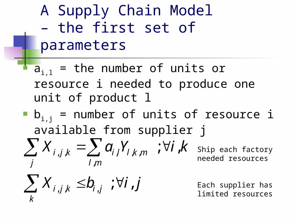
A Supply Chain Model – the first set of parameters

ai,l = the number of units or resource i needed to produce one unit of product l

bi,j = number of units of resource i available from supplier j

, , , , ,,

, , ,

; ,

; ,

i j k i l l k mj l m

i j k i jk

X a Y i k

X b i j

Ship each factoryneeded resources

Each supplier haslimited resources

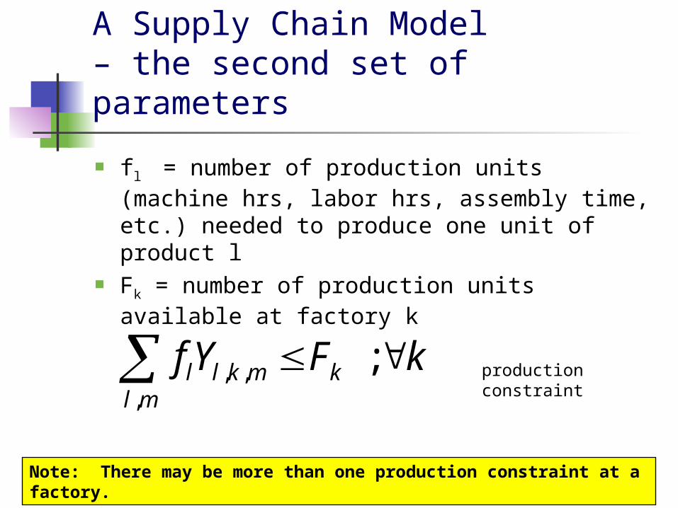
A Supply Chain Model – the second set of parameters

fl = number of production units (machine hrs, labor hrs, assembly time, etc.) needed to produce one unit of product l

Fk = number of production units available at factory k

, ,,

;l l k m kl m

f Y F k productionconstraint

Note: There may be more than one production constraint at a factory.

A Supply Chain Model – the third set of parameters

Dl,m = demand for product l by customer m

, , , ; ,l k m l mk

Y D l m I have a big demand for product l.

A Request…Could you make your so

called supply chain model come alive with a real world

example? My brother, Thomas Maytow, is owner of a cannery. What can your

model do for him?

Pat Maytow, a fruit picker.

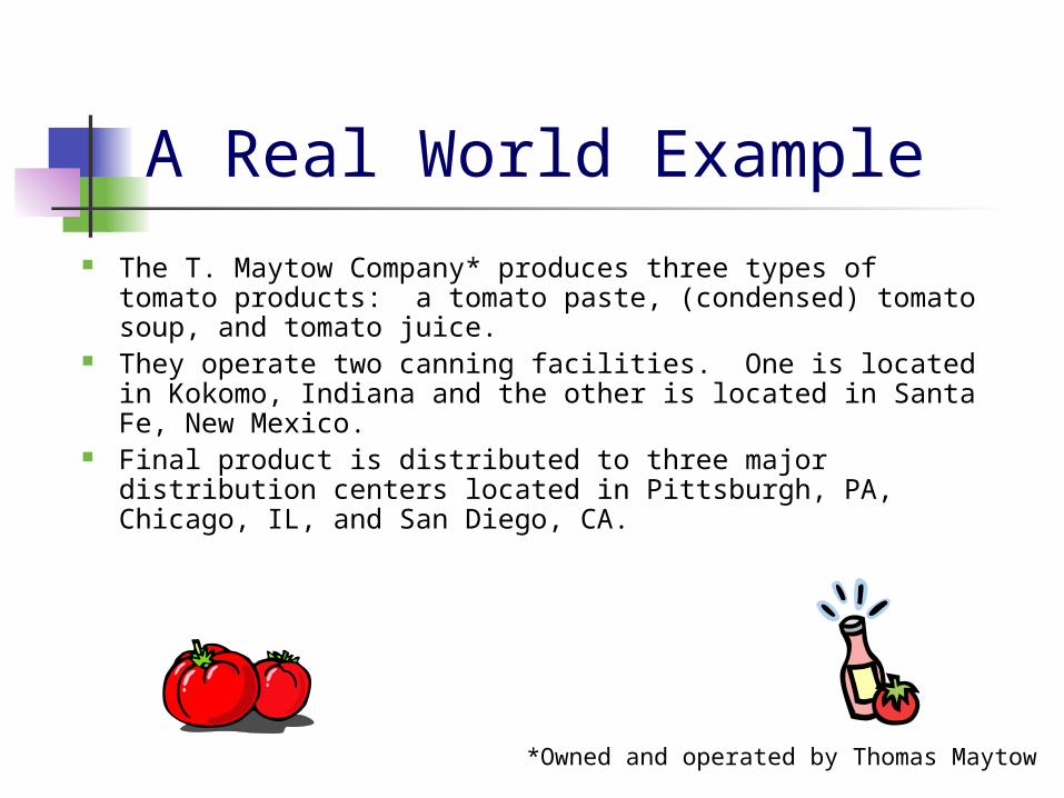
A Real World Example The T. Maytow Company* produces three types of tomato

products: a tomato paste, (condensed) tomato soup, and tomato juice.

They operate two canning facilities. One is located in Kokomo, Indiana and the other is located in Santa Fe, New Mexico.

Final product is distributed to three major distribution centers located in Pittsburgh, PA, Chicago, IL, and San Diego, CA.

*Owned and operated by Thomas Maytow

The Suppliers

There are three varieties of tomatoes used in production:

Roma tomatoes Plum tomatoes Beefsteak tomatoes

There are two major suppliers: Taste of the World (Morristown, New Jersey) imported

from tomato fields near Naples, Italy Sierra Quality Canners from California's central valley

Tomato Distribution A typical tomato truck holds 50,000

pounds of tomatoes, which is about 300,000 tomatoes. (6 X 50,000)

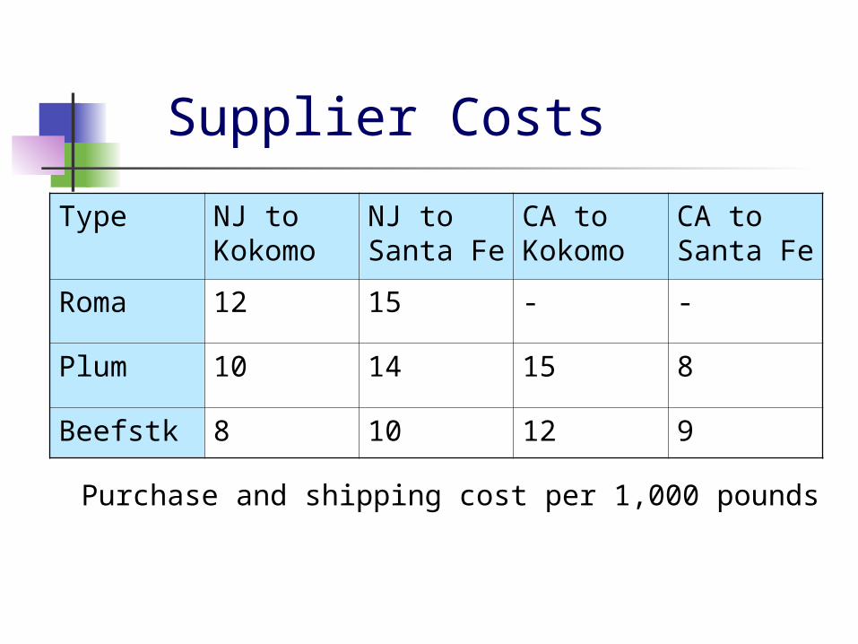
Supplier Costs

Type NJ to Kokomo

NJ to Santa Fe

CA to Kokomo

CA to Santa Fe

Roma 12 15 - -

Plum 10 14 15 8

Beefstk 8 10 12 9

Purchase and shipping cost per 1,000 pounds

Supplier Output

Type Roma Plum Beefstk

NJ 140 100 140

CA - 120 150

1,000 pounds per week

Production & Distribution Costs

Kokomo Paste

Santa Fe Paste

Kokomo Soup

Santa Fe Soup

Kokomo juice

Santa Fe juice

Pgh 8 9 6 7 9 10

Chi 10 11 8 9 11 12

SD 12 10 10 8 13 12

$ per canner load

Tomato Production Tomato Paste - an average of 35 pounds of tomatoes

is needed per canner load of 7 quarts; an average of 21 pounds is needed per canner load of 9 pints. A bushel yields 10 to 12 quarts of sauce.

Tomato Soup - an average of 26 pounds of tomatoes is needed per canner load of 7 quarts; an average of 18 pounds is needed per canner load of 9 pints. A bushel yields 12 to 14 quarts of sauce.

Tomato Juice - An average of 23 pounds of tomatoes is needed per canner load of 7 quarts, or an average of 14 pounds per canner load of 9 pints. A bushel yields 15 to 18 pounds per canner load of 9 pints. A bushel yields 15 to 18 quarts of juice.

Production Requirements*

Paste Soup Juice

Roma 12 - 8

Plum 8 8 15

Beefstk 15 18 -

Total 35 26 23

Pounds of tomatoes per canner load (7 quarts)

*The actual blends of tomato variety into finished product is proprietary

Plant Capacities

Plant Capacity

Kokomo 10,000

Santa Fe 14,000

capacity in canner loads (7 quarts) per week

Distribution Center Requirements

Paste Soup juice

Pgh 2,000 3,000 500

Chi 1,000 4,000 1,500

SD 5,000 2,000 3,000

canner loads (7 quarts) per week

The Decision Variables

Let Xi,j,k = the number of tomatoes in 1,000 pounds of type i shipped from supplier j to factory k

i = roma, plum, beefsteakj = NJ, CAk = Kokomo, Santa Fe

Let Yl,k,m = the number of canner loads of product l produced in factory k for distribution center m

l = paste, soup, juicem = Pgh, Chi, SD

The Objective FunctionMin 12XR_NJ_K + 10XP_NJ_K+ 8XB_NJ_K + 15XR_NJ_S + 14XP_NJ_S + 10XB_NJ_S

+ 15XP_CA_K+ 12XB_CA_K + 8XP_CA_S+ 9XB_CA_S

+8YP_K_PGH + 6YS_K_PGH + 9YJ_K_PGH +9YP_S_PGH + 7YS_S_PGH + 10YJ_S_PGH

+10YP_K_CHI + 8YS_K_CHI + 11YJ_K_CHI +11YP_S_CHI + 9YS_S_CHI + 12YJ_S_CHI

+ 12YP_K_SD + 10YS_K_SD + 13YJ_K_SD +10YP_S_SD + 8YS_S_SD + 12YJ_S_SD

Supplier constraints

East Coast Supplier:XR_NJ_K + XR_NJ_S < 140XP_NJ_K + XP_NJ_S < 100XB_NJ_K + XB_NJ_S < 140

West Coast Supplier:XP_CA_K + XP_CA_S < 120XB_CA_K + XB_CA_S < 150

Legend X variables

first indexR – RomaP – PlumJB– Beefsteak

middle indexNJ – New Jersey supplierCA – California supplier

last indexK – Kokomo plantS – Santa Fe plant

units in 1,000 lb of tomatoes

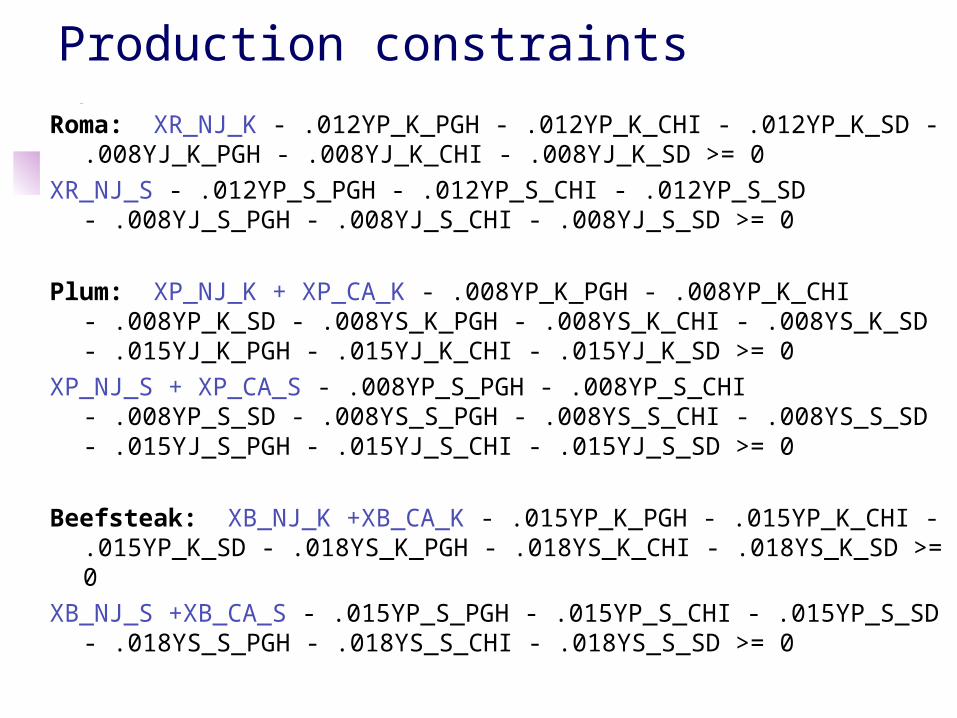
Production constraints

Roma: XR_NJ_K - .012YP_K_PGH - .012YP_K_CHI - .012YP_K_SD - .008YJ_K_PGH - .008YJ_K_CHI - .008YJ_K_SD >= 0

XR_NJ_S - .012YP_S_PGH - .012YP_S_CHI - .012YP_S_SD - .008YJ_S_PGH - .008YJ_S_CHI - .008YJ_S_SD >= 0

Plum: XP_NJ_K + XP_CA_K - .008YP_K_PGH - .008YP_K_CHI - .008YP_K_SD - .008YS_K_PGH - .008YS_K_CHI - .008YS_K_SD - .015YJ_K_PGH - .015YJ_K_CHI - .015YJ_K_SD >= 0

XP_NJ_S + XP_CA_S - .008YP_S_PGH - .008YP_S_CHI - .008YP_S_SD - .008YS_S_PGH - .008YS_S_CHI - .008YS_S_SD - .015YJ_S_PGH - .015YJ_S_CHI - .015YJ_S_SD >= 0

Beefsteak: XB_NJ_K +XB_CA_K - .015YP_K_PGH - .015YP_K_CHI - .015YP_K_SD - .018YS_K_PGH - .018YS_K_CHI - .018YS_K_SD >= 0

XB_NJ_S +XB_CA_S - .015YP_S_PGH - .015YP_S_CHI - .015YP_S_SD - .018YS_S_PGH - .018YS_S_CHI - .018YS_S_SD >= 0

Production Capacity constraints

Kokomo:YP_K_PGH + YS_K_PGH + YJ_K_PGH + YP_K_CHI

+ YS_K_CHI + YJ_K_CHI + YP_K_SD + YS_K_SD + YJ_K_SD < 10000

Santa Fe:YP_S_PGH + YS_S_PGH + YJ_S_PGH + YP_S_CHI +

YS_S_CHI + YJ_S_CHI+ YP_S_SD + YS_S_SD + YJ_S_SD < 14000

in canner loads

Distribution Center Requirements

Pittsburgh:YP_K_PGH + YP_S_PGH > 2000YS_K_PGH + YS_S_PGH > 3000YJ_K_PGH + YJ_S_PGH > 500

Chicago:YP_K_CHI + YP_S_CHI > 1000YS_K_CHI + YS_S_CHI > 4000YJ_K_CHI + YJ_S_CHI > 1500

San Diego:YP_K_SD + YP_S_SD > 5000YS_K_SD + YS_S_SD > 2000YJ_K_SD + YJ_S_SD > 3000

Legend Y variables

first indexP – pasteS – soupJ – juice

middle indexK – KokomoS – Santa Fe

units in canner loads

The Glorious SolutionMin Cost per week =

$207,160.80

VARIABLE VALUE XR_NJ_K 49.777775 XP_NJ_K 92.055557 XB_NJ_K 140.000000 XR_NJ_S 86.222229 XP_NJ_S 0.000000 XB_NJ_S 0.000000 XP_CA_K 0.000000 XB_CA_K 0.000000 XP_CA_S 118.944450 XB_CA_S 141.999985 YP_K_PGH 2000.0000 YS_K_PGH 3000.0000 YJ_K_PGH 500.00000 YP_S_PGH 0.000000 YS_S_PGH 0.000000

VARIABLE VALUE

YJ_S_PGH 0.000000 YP_K_CHI 1000.0000 YS_K_CHI 2277.778076 YJ_K_CHI 1222.221924 YP_S_CHI 0.000000 YS_S_CHI 1722.221924 YJ_S_CHI 277.778046 YP_K_SD 0.000000 YS_K_SD 0.000000 YJ_K_SD 0.000000 YP_S_SD 5000.00000 YS_S_SD 2000.00000 YJ_S_SD 3000.00000

More of the Glorious Solution

Kokomo Paste

Santa Fe Paste

Kokomo Soup

Santa Fe Soup

Kokomo juice

Santa Fe juice

Pgh 2000 3000 500

Chi 1000 2277.78 1722.22 1222.22 277.78

SD 5000 2000 3000

Type NJ to Kokomo

NJ to Santa Fe

CA to Kokomo

CA to Santa Fe

Roma 49.78 86.22

Plum 92.06 118.94

Beefstk 140 142.0

Final Product (weekly canner loads):

Resources (weekly 1,000 lb of tomatoes):

The End of the Supply Chain Model

The bottom line:The supply chain locks in money!

Goods and services flowingthrough the supply pipeline