i

Supply Chain Management in Disaster Response

Final Project Report

Grant DTRT07-G-0003

Mid-Atlantic Universities Transportation Center

By:

Ali Haghani Professor & Chairman

Abbas M. Afshar PhD Candidate

Department of Civil & Environmental Engineering

University of Maryland College Par, MD 20742

September 2009

ii

Supply Chain Management in Disaster Response

ABSTRACT

In today’s society that disasters seem to be striking all corners of the United States

and the globe, the importance of emergency management is undeniable. Much human

loss and unnecessary destruction of infrastructure can be avoided with more foresight

and specific planning. During emergencies various aid organizations often face

significant problems of transporting large amounts of many different commodities

including food, clothing, medicine, medical supplies, machinery, and personnel from

different points of origin to different destinations in the disaster areas. The

transportation of supplies and relief personnel must be done quickly and efficiently to

maximize the survival rate of the affected population and minimize the cost of such

operations.

Federal Emergency Management Agency (FEMA) is the primary organization for

preparedness and response to federal level disasters in the United States. FEMA has a

very complex logistics structure to provide the disaster victims with critical items

after a disaster strike which involves multiple organizations and spreads all across the

country. Unfortunately, inadequate response to hurricanes Katrina and Rita showed

the critical need for better mechanisms in emergency operations. Initial research in

this area showed that this is an emerging field and there are great potentials for

research in emergency logistics and disaster response.

The goal of this research is to develop a comprehensive model that describes the

integrated supply chain operations in response to natural disasters. An integrated

model that captures the interactions between different components of the supply chain

is a very valuable tool. It is ideal to have a model that controls the flow of relief

commodities from the sources through the chain and until they are delivered to the

hands of recipients. This research will offer a model that not only considers details

such as vehicle routing and pick up or delivery schedules; but also considers finding

the optimal location for temporary facilities as well as considering the capacity

constraints for each facility and the transportation system. Such a model provides the

iii

opportunity for a centralized operation plan that can eliminate delays and assign the

limited resources in a way that is optimal for the entire system.

Emergency response operation is a dynamic and very time sensitive operation. A

mathematical model at the operational level is needed that can be used in the critical

hours and days immediately after the disaster strikes. Such a model is a unique tool

that can also be used at strategic level or planning level analysis. It is a very

complicated task and to date, there is no study in the literature that has addressed this

problem sufficiently.

This research also aims at developing optimization algorithms and heuristics to solve

the proposed model and find applicable solutions to decrease human sufferings in the

most economically sensible way. The algorithms need to be fast so that the results can

be used in the initial response phase and also as the situation changes in the highly

dynamic environment after the disaster.

Finally, a comprehensive series of numerical analysis is performed to evaluate the

proposed model and solution algorithms. The numerical analysis shows the required

details for model implementation. A range of analysis is conducted to investigate the

effect of different parameters on the mathematical model. Overall, the numerical

analysis confirms the applicability of the proposed model in real-world like scenarios.

Also, it is shown that the model size and complexity grows rapidly in case of large-

scale disasters which emphasize the need and importance of fast and efficient solution

algorithms. At the end, conclusions and directions for future research are discussed.

iv

Table of Contents

Table of Contents ......................................................................................................... iv Glossary of Terms ......................................................................................................... v Chapter 1: Introduction ................................................................................................. 1

1.1. Disasters .................................................................................................1 1.1.1 Definitions ....................................................................................... 1 1.1.2 Numbers and Trends ....................................................................... 3

1.2. Emergency Management ........................................................................5 1.3. Federal Emergency Management Agency .............................................8 1.4. FEMA’s Logistics Supply Chain .........................................................12 1.5. Motivation and Objective of the Research ...........................................15 1.6. Contributions of the research ...............................................................16 1.7. Organization of the report ....................................................................17

Chapter 2: Literature review ....................................................................................... 18 2.1. Supply Chain Management ..................................................................18

2.1.1. Facility Location Problem .............................................................21 2.1.2. Vehicle Routing Problem ..............................................................27

2.2. Commercial Supply Chain versus Emergency Response Logistics .....31 2.3. Logistics in Disaster Response .............................................................34

2.3.1 Early Ages ......................................................................................34 2.3.2 Recent Studies ................................................................................35

2.4. Conclusions ..........................................................................................38 Chapter 3: Problem Description and Formulation .......................................................39

3.1. Problem Description .............................................................................39 3.2. Time-Space Network ............................................................................42 3.3. Modeling Approach ..............................................................................45 3.4 Assumptions ..........................................................................................46 3.5. Mathematical model .............................................................................47

3.5.1 Notations ........................................................................................47 3.5.2 Parameters ......................................................................................48 3.5.3 Decision Variables .........................................................................49 3.5.4 Objective Function .........................................................................50 3.5.5 Constraints .....................................................................................51

3.6. Summary ..............................................................................................55 Chapter 4: Numerical Study........................................................................................ 56

4.1. Design of Sample Problems .................................................................56 4.2. Generating Formulation and Commercial Solver ................................66 4.3. Numerical Results and Analysis ...........................................................67 4.4. Summary ..............................................................................................77

Chapter 5: Conclusions and Future Directions ........................................................... 78 Chapter 6: Bibliography .............................................................................................. 81

v

Glossary of Terms

CRED Center for Research on the Epidemiology of Disasters

CSS Commercial Storage Site

DHS Department of Homeland Security

DLA Defense Logistics Agency

ESF Emergency Support Function

FEMA Federal Emergency Management Agency

FOSA Federal Operational Staging Area

GSA General Services Administration

LC Logistics Center

MOB Mobilization centers

NRF National Response Framework

PAHO Pan American Health Organization

POD Point of Distribution

SSA State Staging Area

WHO World Health Organization

1

Chapter 1: Introduction

1.1. Disasters

1.1.1 Definitions

The term “disaster” is usually applied to a breakdown in the normal functioning of a

community that has a significant adverse impact on people, their works, and their

environment, overwhelming local response capacity. This situation may be the result of a

natural event such as a hurricane or earthquake; or it may be the result of human activities

(PAHO 2001). Some organizations make a distinction between “disasters”—the result of

natural phenomena—and “complex emergencies” that are the product of armed conflicts

or large-scale violence and often lead to massive displacements of people, famine, and

outflows of refugees.

A disaster, as defined by the World Health Organization (WHO), is any occurrence that

causes damage, destruction, ecological disruption, loss of human life, human suffering,

deterioration of health and health services on a scale sufficient to warrant an

extraordinary response from outside the affected community or area. The American Red

Cross defines a disaster as an occurrence or situation that causes human suffering or

creates human needs that the victims cannot alleviate without assistance. Earthquakes,

hurricanes, tornadoes, volcanic eruptions, wild fires, floods, blizzard, drought, terrorism,

chemical spills and nuclear accidents are included among the causes of disasters, and all

have significant devastating effects in terms of human injuries and property damage.

Alexander (1999) defines natural disaster as some rapid, instantaneous or profound

impact of the natural environment upon the socio-economic system. He also recommends

Turner’s (1976) definition of natural disaster as “an event, concentrated in time and

space, which threatens a society or subdivision of a society with major unwanted

consequences as a result of the collapse of precautions which had previously been

culturally accepted as adequate”.

2

Center for Research on the Epidemiology of Disasters (CRED), collaborating center with

WHO and United Nations, defines disaster as “A situation or event, which overwhelms

local capacity, necessitating a request to national or international level for external

assistance; an unforeseen and often sudden event that causes great damage, destruction

and human suffering”. (CRED 2007)

The official definition of disasters in the United States is presented in the Stafford Act.

The Robert T. Stafford Disaster Relief and Emergency Assistance Act is the primary

legislation in the United States authorizing the federal government to provide disaster

assistance to states, local governments, families, and individuals. The Stafford Act

defines a disaster as

“Any natural catastrophe (including hurricane, tornado, storm, high

water, wind driven water, tidal wave, tsunami, earthquake, volcanic

eruption, landslide, mudslide, snowstorm or drought), or, regardless of

cause, any fire, flood or explosion, in any part of the United States, which

in the determination of the President causes damage of sufficient severity

and magnitude to warrant major disaster assistance under this Act to

supplement the efforts and available resources of States, local

governments, and disaster relief organizations, in alleviating the damage,

loss, hardship, or suffering caused thereby.”

As these definitions indicate, a disaster is a “catastrophe” of such magnitude and severity

that the capacities of states and local governments are overwhelmed. So the threshold for

determining what constitutes a disaster depends upon the availability of resources and

capabilities of responding communities. Consequently, a disaster can be prevented by

increasing the capacity of responding organizations.

3

1.1.2 Numbers and Trends

From a global perspective, the number of natural disasters is increasing every year. For

example in 2005, there have been 489 country-level disasters affecting 127 countries

around the globe resulting in 104,698 people killed and 160 million affected. For the

same year of 2005, the economic damage estimate varies from 159 billion to 210 billion

in US dollars. Because of the population growth and new developments in risk prone

regions, the exposure of the human kind to the natural disasters is increasing even more.

Figure 1.1 shows the number of reported natural disasters around the globe from 1980 to

2007. A least-square linear regression trend-line is drawn to better illustrate the overall

pattern. Trend-line in Figure 1.1 shows that in spite of fluctuations due to cyclic or

seasonal patterns, the average number of disasters is growing in long-term. During 1980s

number of disasters is around 180 per year on average. In 1990s, the average number of

disasters increases to around 300 per year. And in the 2000-2007 period, these numbers

are around 460 disasters per year which indicates a dramatic increase. An increase of this

magnitude can be explained partially by the global warming theory, and partially by the

attention of the media which has increased the numbers of reported disasters all over the

world.

As the number of disasters increases every year, more people are affected by these

disasters. Figure 1.2 illustrates the number of victims of natural or man-made disasters in

the last twenty years. The number of victims includes the people killed, injured, lost their

homes or evacuated as a direct result of the disaster. As can bee seen in figure 1.2, the

number of victims has higher fluctuations over the years. However, the trend-line shows

a slow increase in the average number of peoples affected each year over time. The

number of victims is generally between 100 million and 400 million per year. An

exceptionally high number in 2002 is due to a drought solely affecting 360 million in

India and China and a major wind storm and flood affecting 160 million people in China.

4

Figure 1.1- Number of reported natural disasters per year around the world (CRED)

Figure 1.2- Number of Victims of natural disasters per year (CRED)

Another important factor is the monetary cost of natural disasters. Figure 1.3 shows the

amounts of global economical damage caused by natural disaster from 1980 to 2007. The

0

100

200

300

400

500

600

1980 1983 1986 1989 1992 1995 1998 2001 2004 2007

Dis

aste

rs p

er y

ear

Number of Natural disasters

0

100

200

300

400

500

600

700

1980 1983 1986 1989 1992 1995 1998 2001 2004 2007

Per

son

Aff

ecte

d (

Mill

ion

)

Total Number of people affected

5

average cost per year is $45 billion from 1980 to 1999. However, for 2000 to 2007

period, the average cost is more than $80 billion per year. The linear trend-line shows this

increase in the economical damage of the natural disasters over time. Two major disasters

affecting the trend are the Kobe earthquake in 1995 and hurricane Katrina in 2005.

Figure 1.3- Economic damage of the natural disasters over time (CRED)

1.2. Emergency Management

Emergency management (or disaster management) is the discipline of avoiding risks and

dealing with risks (Haddow et al. 2007). No country and no community are immune from

the risk of disasters. However, it is possible to prepare for, respond to and recover from

disasters and limit the destructions to a certain degree. Emergency management is a

discipline that involves preparing for disaster before it happens, responding to disasters

immediately, as well as supporting, and rebuilding societies after the natural or human-

made disasters have occurred.

Emergency management is a continuous process. It is essential to have comprehensive

emergency plans and evaluate and improve the plans continuously. The related activities

0

50

100

150

200

250

1980 1983 1986 1989 1992 1995 1998 2001 2004 2007

Bill

ion

US

Do

llars

Estimated Damage Cost of Natural Disasters

6

are usually classified as four phases of Preparedness, Response, Recovery, and

Mitigation. Figure 1.4 illustrates the order of these phases according to the onset of the

disaster. Appropriate actions at all points in the cycle lead to greater preparedness, better

warnings, reduced vulnerability or the prevention of disasters during the next iteration of

the cycle.

Figure 1.4- Four Phases of Emergency Management Cycle

Some of the main activities during four phases of emergency management cycle are

summarized below:

Preparedness

Activities to improve the ability to respond quickly in the immediate

aftermath of an incident.

Includes development of response procedures, design and installation of

warning systems, evacuation planning, exercises to test emergency

operations, and training of emergency personnel.

Response

Activities during or immediately following a disaster to meet the urgent

needs of disaster victims.

7

Involves mobilizing and positioning emergency supplies, equipment and

personnel; includes time-sensitive operations such as search and rescue,

evacuation, emergency medical care, food and shelter programs, and

bringing damaged services and systems back online.

Recovery

Actions that begin after the disaster, when urgent needs have been met.

Recovery actions are designed to put the community back together

Include repairs to roads, bridges, and other public facilities, restoration of

power, water and other municipal services, and other activities to help

restore normal operations to a community.

Mitigation

Activities that prevent a disaster, reduce the chance of a disaster happening,

or lessen the damaging effects of unavoidable disasters and emergencies.

Includes engineering solutions such as dams and levees; land-use planning

to prevent development in hazardous areas; protecting structures through

sound building practices and retrofitting; acquiring and relocating damaged

structures; preserving the natural environment to serve as a buffer against

hazard impacts; and educating the public about hazards and ways to reduce

risk.

Emergency management process needs the cooperation of all individuals, groups, and

communities to be successful. When a major disaster happens, emergency management

agencies from all over the world work with governments and non-governmental

organizations in an effort to decrease the impact of the disaster. Humanitarian

organizations such as American Red Cross, CARE USA, Catholic Relief Services,

International Committee of the Red Cross, International Federation of Red Cross and Red

Crescent Societies, International Rescue Committee, UNICEF, World Bank, and World

Food Programme are among the organizations that work with different national

organizations inside the affected countries to provide humanitarian aids.

8

In the United States, the Federal Emergency Management Agency (FEMA) is the main

agency to deal with emergencies. They work in partnership with other organizations that

are part of the national emergency management system. These partners include state and

local emergency management agencies, 27 other federal agencies and the American Red

Cross. More details on FEMA’s structure and operations are introduced in the following

section.

1.3. Federal Emergency Management Agency

Federal Emergency Management Agency (FEMA) is the main organization responsible

for dealing with federal level emergencies in the United States. It was initially created in

1979 as an independent organization but On March 1st, 2003 FEMA became part of the

U.S. Department of Homeland Security (DHS) along with 22 other government agencies.

FEMA is a relatively small agency with around 2,600 full time employees but it can

mobilize nearly 7000 temporary disaster assistance employees to respond to disasters.

Besides the headquarters in Washington D.C., FEMA has ten regional offices across the

country to coordinate with its state and local government counterparts and with nonprofit

and for-profit organizations.

The primary mission of FEMA is

“To reduce the loss of life and property and protect the Nation from all

hazards, including natural disasters, acts of terrorism, and other man-

made disasters, by leading and supporting the Nation in a risk-based,

comprehensive emergency management system of preparedness,

protection, response, recovery, and mitigation.” (www.fema.gov)

FEMA’s Strategic Plan for Fiscal Years 2008-2013 declares the vision of the

organization as “The Nation’s Preeminent Emergency Management and Preparedness

Agency”. The Plan establishes strategic goals, objectives, and strategies to fulfill

FEMA’s vision. The strategic goals of the agency are to:

9

1. Lead an integrated approach that strengthens the Nation’s ability to address

disasters, emergencies, and terrorist events

2. Deliver easily accessible and coordinated assistance for all programs

3. Provide reliable information at the right time for all users

4. FEMA invests in people and people invest in FEMA to ensure mission success

5. Build public trust and confidence through performance and stewardship

One of the important documents that define the principles, roles, and structures of FEMA

is the National Response Framework (NRF). NRF replaced its older version called

National Response Plan on March 22, 2008. NRF presents the guiding principles that

enable all response partners to prepare for and provide a unified national response to

disasters and emergencies. It describes how communities, tribes, states, the federal

government, private-sectors, and nongovernmental partners work together to coordinate

national response. Following the guidelines of NRF are essential to establish a

comprehensive, national, all-hazards approach for disaster response in the United States.

NRF main documents are supplemented by important annexes called Emergency Support

Functions (ESF). The ESFs provide the structure for coordinating Federal interagency

support for a Federal response to an emergency. They are mechanisms for grouping

functions most frequently used to provide Federal support to States and Federal-to-

Federal support, both for declared disasters and emergencies under the Stafford Act and

for non-Stafford Act incidents. Table 1.1 gives a summery of the 15 ESFs currently

present in the NRF. More Information on the National Response Framework including

Documents, Annexes, References and Briefings/Trainings can be accessed through the

NRF Resource Center at www.fema.gov/nrf .

10

Table 1.1 Emergency Support Function Annexes of the National Response Framework ESF Scope

ESF #1 – Transportation

Aviation management and control; Transportation safety Restoration/recovery of transportation infrastructure; Movement restrictions; Damage and impact assessment

ESF #2 – Communications

Coordination with telecommunications and information technology industries; Restoration and repair of telecommunications infrastructure Protection, restoration, and sustainment of national cyber and information technology resources; Oversight of communications within the Federal incident management and response structures

ESF #3 – Public Works and Engineering

Infrastructure protection and emergency repair; Infrastructure restoration; Engineering services and construction management; Emergency contracting support for life-saving and life-sustaining services

ESF #4 – Firefighting

Coordination of Federal firefighting activities; Support to wild land, rural, and urban firefighting operations

ESF #5 – Emergency Management

Coordination of incident management and response efforts; Issuance of mission assignments; Resource and human capital; Incident action planning; Financial management

ESF #6 –Housing, and Human Services

Mass care; Emergency assistance; Disaster housing; Human services

ESF #7 – Logistics Management

Comprehensive, national incident logistics planning, management, and sustainment capability; Resource support (facility space, office equipment and supplies, contracting services, etc.)

ESF #8 – Public Health

Public health; Medical and Mental health services; Mass fatality management

ESF #9 – Search and Rescue

Life-saving assistance Search and rescue operations

ESF #10 – Hazardous Materials

Oil and hazardous materials (chemical, biological, radiological, etc.) response; Environmental short- and long-term cleanup

ESF #11 – Agriculture and Natural Resources

Nutrition assistance; Animal and plant disease and pest response; Food safety and security; Natural and cultural resources and historic properties protection and restoration; Safety and well-being of household pets

ESF #12 – Energy Energy infrastructure assessment, repair, and restoration; Energy industry utilities coordination; Energy forecast

ESF #13 – Public Safety and Security

Facility and resource security; Security planning and technical resource assistance; Public safety and security support; Support to access, traffic, and crowd control

ESF #14 – Long-Term Recovery

Long-term community recovery assistance to States, local governments, and the private sector Analysis and review of mitigation program implementation

ESF #15 – External Affairs

Emergency public information and protective action guidance; Media and community relations; Congressional and international affairs; Tribal and insular affairs

11

Emergency Support Function #7, Logistics Management and Resource Support Annex,

describes the roles and responsibilities of FEMA and General Services Administration

(GSA) to jointly manage a supply chain that provides relief commodities to the victims.

Based on ESF #7, FEMA is the primary agency for Logistics Management and is

responsible for:

Material management that includes determining requirements, sourcing, ordering

and replenishment, storage, and issuing of supplies and equipment.

Transportation management that includes equipment and procedures for moving

material from storage facilities and vendors to incident victims, particularly with

emphasis on the surge and sustainment portions of response. Transportation

management also includes providing services to requests from other Federal

organizations.

Facilities management that includes the location, selection, and acquisition of

storage and distribution facilities. These facilities include Logistics Centers,

Mobilization Centers, and Federal Operations Staging Areas.

Personal property management and policy and procedures guidance for

maintaining accountability of material and identification and reutilization of

property acquired to support a Federal response operation.

Management of Electronic Data Interchange to provide end-to-end visibility of

response resources.

Planning and coordination with internal and external customers and other supply

chain partners in the Federal and private sectors for improving the delivery of

goods and services to the customer.

The next section introduces the components of FEMA’s logistics operations and

describes the structure of FEMA’s supply chain.

12

1.4. FEMA’s Logistics Supply Chain

FEMA has a complicated and special structure for its supply chain. There are seven main

components in the supply chain to provide relief commodities for disaster victims that are

briefly described here:

1. FEMA Logistics Centers (LC) - permanent facilities that receive, store, ship,

and recover disaster commodities and equipment. FEMA has a total of 9 logistics

centers:

4 Continental United States centers containing general commodities

located at Atlanta, Georgia; Ft. Worth, Texas; Frederick, Maryland; and

Moffett Field, California.

3 Off-shore centers containing general commodities located in Hawaii,

Guam, and Puerto Rico.

2 Continental United States centers containing special products such as

computers, office electronic equipment, medical and pharmaceutical

caches located in Cumberland, Maryland and Berryville, Virginia.

Examples of disaster relief commodities include ice, water, meals ready to eat (MREs),

blankets, cots, flashlights, tarps, sleeping bags and tents. Disaster relief equipments

include emergency generators, personal toilet kits, and refrigerated vans.

2. Commercial Storage Sites (CSS) - permanent facilities that are owned and

operated by private industry and store commodities for FEMA. Freezer storage

space for ice is an example.

3. Other Federal Agencies Sites (VEN) - representing vendors from whom

commodities are purchased and managed. Examples are Defense Logistics

Agency (DLA) and General Services Administration (GSA).

4. Mobilization (MOB) Centers - temporary federal facilities in theater at which

commodities, equipment and personnel can be received and pre-positioned for

13

deployment as required. In MOBs commodities remain under the control of

FEMA logistics headquarter and can be deployed to multiple states. MOBs are

generally projected to have the capacity to hold 3 days of supply commodities.

5. Federal Operational Staging Areas (FOSAs) - temporary facilities at which

commodities, equipment and personnel are received and pre-positioned for

deployment within one designated state as required. Commodities are under the

control of the Operations Section of the Joint Field Office (JFO) or Regional

Response Coordination Center (RRCC). Commodities are usually being supplied

from MOB Centers, Logistics Centers or direct shipments from vendors. FOSAs

are generally projected to hold 1 to 2 days of commodities.

6. State Staging Areas (SSA) - temporary facilities in the affected state at which

commodities, equipment and personnel are received and pre-positioned for

deployment within that state. Title transfers for delivered federal commodities and

cost sharing are initiated in SSAs.

7. Points of Distribution (PODs) Sites - temporary local facilities in the disaster

area at which commodities are distributed directly to disaster victims. PODs are

operated by the affected state.

Figure 1.5 better illustrates this structure. At the top of the pyramid there are 3 types of

facilities namely FEMA Logistics Centers, Commercial Storage Sites, and Other Federal

Agencies or Vendors. These permanent facilities store and ship commodities and

equipment and are considered as “sources” in the chain. Mobilization Centers, Federal

Operational Staging Areas, and State Staging Areas are 3 types of facilities that mainly

play the role of transshipment points. These are temporary facilities at which

commodities, equipment and personnel are received and pre-positioned for deployment to

the lower levels. At the end, Points of Distribution Sites are temporary local facilities at

which commodities are received and distributed directly to disaster victims. PODs can be

local schools, churches, or big parking lots in the affected area.

14

Figure 1.5 FEMA’s Supply Chain Structure

Even this simplified presentation of the FEMA’s logistics supply chain indicates the

complex structure of the system. Finding the optimal sites for 4 levels of temporary

facilities is a complicated location finding problem. Delivering several types of

commodities to disaster victims is a multicommodity capacitated network flows problem.

Optimizing the movement of vehicles in the network is a dynamic vehicle routing

problem with mixed pick up and delivery operations. Usually more than one

transportation mode is used in disaster response operations which makes the problem a

multimodal transportation problem. Other characteristics that make the problem unique

include, but are not limited to, importance of quick response and fast delivery, shortage

of supply versus overwhelming demands, insufficient capacity of facilities and

transportation system, and dynamic environment of the emergency situations.

Logistics Centers

MOB Centers

State Staging

Area

POD

Commercial Storage Sites

State Staging

Area

POD POD POD

Vendors

FOSAs

15

1.5. Motivation and Objective of the Research

In today’s society that disasters seem to be striking all corners of the United States and

the globe, the importance of emergency management is undeniable. Much human loss

and unnecessary destruction of infrastructure can be avoided with more foresight and

specific planning as well as a precise execution. In a world where resources are stretched

to the limit and the question of humanitarian relief seems too often to be tied with

economical considerations, better designs and operations are urgently needed to help save

thousands of lives and millions of dollars.

The question is how to respond to natural disasters in the most efficient manner to

minimize the loss of life and maximize the efficiency of the rescue operations. In case of

these emergencies various organizations often face significant problems of transporting

large amounts of many different commodities including food, clothing, medicine,

medical supplies, machinery, and personnel from different points of origin to different

destinations in the disaster areas. The transportation of supplies and relief personnel must

be done quickly and efficiently to maximize the survival rate of the affected population

and minimize the cost of such operations.

Federal Emergency Management Agency (FEMA) is the primary organization for

preparedness and response to federal level disasters in the United States. Unfortunately,

inadequate response to hurricanes Katrina and Rita showed the critical need for better

mechanisms in emergency operations. Initial research in this area shows that this is an

emerging field and there are great potentials for research in emergency logistics and

disaster response.

FEMA has a very complex logistics structure to provide the disaster victims with critical

items after a disaster strike which involves multiple organizations and spreads across the

country. The goal of this research is to develop a comprehensive model that describes the

integrated supply chain operations in response to natural disasters. An integrated model

that captures the interactions between different components of the supply chain is a very

16

valuable tool. It is ideal to have a model that controls the flow of relief commodities from

the sources through the chain and until they are delivered to the hands of recipients. Such

a model provides the opportunity for a centralized operation plan that can eliminate

delays and assign the limited resources in a way that is optimal for the entire system.

1.6. Contributions of the research

Emergency response operation is a dynamic and very time sensitive operation. This

research will offer a model that not only considers details such as vehicle routing and

pick up or delivery schedules; but also considers finding the optimal location for

temporary facilities as well as considering the capacity constraint for each facility and the

transportation system. A mathematical model at the operational level is needed that can

be used in the critical hours and days immediately after the disaster strikes. Such a model

is a unique tool that can also be used at strategic level or planning level analysis. It is a

very complicated task and up to date, there is no study in the literature that has addressed

this problem sufficiently.

This research also aims at developing optimization algorithms and heuristics to solve the

proposed model and find applicable solutions to decrease human sufferings in the most

economically sensible way. The algorithms need to be fast so that the results can be used

in the initial response phase and also as the situation changes in the highly dynamic

environment after the disaster.

This research extends the state-of-the-art by presenting a model at the operational level

which describes the details of supply chain operations in major emergency management

agencies such as FEMA, in response to immediate aftermath of a large scale disaster.

Development of fast and efficient solution algorithms and heuristics for the proposed

model will be the other major contribution of this research.

17

1.7. Organization of the report

After introduction, previous works on the logistics of disaster relief operations are

reviewed in chapter 2. The specific problem to be dealt with in this research is introduced

in chapter 3 and then the mathematical formulation of the model is presented. Chapter 4

offers a set of numerical problems to help better understand the mechanics of the model.

Finally in the 5th chapter, the conclusions and directions for future research are discussed.

18

Chapter 2: Literature review

In this section, first some definitions of supply chain and supply chain management

(SCM) in commercial sector are introduced then some of the researches that reviewed the

supply chain studies are summarized. Then, as two main elements of supply chain and

logistics planning, a brief introduction to facility location problem and vehicle routing

problem are presented. Next, the similarities and differences between commercial supply

chain and logistics of disaster response are reviews. Finally, some of the studies specific

to modeling and optimization of logistics in disaster response are provided. This section

concludes with a summary of previews works in this area and the gaps in the literature

that needs to be filled.

2.1. Supply Chain Management

Definition of SCM differs across authors from different fields and there is no explicit and

universal description of supply chain management or its activities in the literature (Tan

2001). The literature is full of buzzwords such as: integrated purchasing strategy,

integrated logistics, supplier integration, buyer-supplier partnerships, supply base

management, strategic supplier alliances, supply chain synchronization and supply chain

management, to address elements or stages of this phenomenon (New, 1997; La Londe

and Masters, 1994).

For example Harland (1996) described supply chain management as managing business

activities and relationships (1) internally within an organization, (2) with immediate

suppliers, (3) with first and second-tier suppliers and customers along the supply chain,

and (4) with the entire supply chain. Scott and Westbrook (1991) and New and Payne

(1995) describe supply chain management as the chain linking each element of the

manufacturing and supply process from raw materials through to the end user, including

several organizational boundaries. SCM begins with the extraction of raw materials or

minerals from the earth, through the manufacturers, wholesalers, retailers, and the final

19

users. Where appropriate, supply chain management also includes recycling or re-use of

the products or materials.

Another definition of supply chain management emerges from the transportation and

logistics literature of the wholesaling and retailing industry, emphasizing the importance

of physical distribution and integrated logistics. There is no doubt that logistics is an

important function of business and is evolving into strategic supply chain management

(New and Payne, 1995). In this definition, the physical transformation of the products is

not a critical component of supply chain management. Its primary focus is the efficient

physical distribution of final products from the manufacturers to the end users in an

attempt to replace inventories with information and reduce transportation costs.

The definition of supply chain (SC) seems to be more common across authors than the

definition of supply chain management (Mentzer et al. 2001). La Londe and Masters

(1994) proposed that a supply chain is a set of firms that pass materials forward. Eksioglu

(2002) defined a supply chain as an integrated process where different business entities

such as suppliers, manufacturers, distributors, and retailers work together to plan,

coordinate, and control the flow of materials, parts, and finished goods from suppliers to

customers. Several independent firms can be involved in manufacturing a product and

placing it in the hands of the end user in a supply chain. For example raw material and

component producers, product assemblers, wholesalers, retailer merchants and

transportation companies are all members of the supply chain.

Beamon (1998) defined supply chain as an integrated manufacturing process where raw

materials are converted into final products, then delivered to customers. At its highest

level, a supply chain is comprised of two basic integrated processes: (1) the Production

Planning and Inventory Control Process, and (2) the Distribution and Logistics Process.

These Processes define the basic framework for the conversion and movement of raw

materials into final products. Figure 2.1 illustrates a simplified picture of supply chain

process.

20

Figure 2.1 Supply chain process (Beamon 1998)

The Production Planning and Inventory Control Process includes the manufacturing and

storage sub-processes and their interfaces. More specifically, production planning

describes the design and management of the entire manufacturing process including raw

material scheduling and acquisition, manufacturing process design and scheduling, and

material handling design and control). Inventory control describes the design and

management of the storage policies and procedures for raw materials, work-in-process

inventories, and usually, final products.

The Distribution and Logistics Process determines how products are retrieved and

transported from the storage warehouse to retailers. These products may be transported to

retailers directly, or may be shipped to distribution facilities first and then being delivered

to the retailers. This process includes the management of inventory retrieval,

transportation, and final product delivery.

These processes interact with one another to produce an integrated supply chain. The

design and management of these processes determine the extent to which the supply

chain works as a unit to meet required performance objectives. Usually in commercial

supply chain, the objective is to minimize cost. However, some have considered a

combination of cost and customer service as the objective.

Suppliers

Manufacturers Storage Facilities Transportation

Distribution Centers

Retailers

Production planning and Inventory Control

Distribution and Logistics

21

For many years, researchers and practitioners have concentrated on the individual

processes and entities within the SC. However, the resent trend is to model and optimize

the SC as a single unified entity. In this approach, operations research (OR) techniques

have shown to be a very useful tool among researchers and practitioners. Typically, a SC

model tries to determine

the transportation modes to be used,

the suppliers to be selected,

the amount of inventory to be held at various locations in the chain,

the number of warehouses to be used, and

the location and capacities of these warehouses.

A more comprehensive review of model and methods in supply chain design and analysis

readers are referred to Beamon (1998) and Tan (2001). In the following subsection of this

chapter, some of the elements of SCM that can be applied in disaster response logistics

are introduced in more details.

2.1.1. Facility Location Problem

One of the most important problems in supply chain management is deciding where to

locate new facilities such as factories, warehouses, distribution centers or retailers to

support the material flow through an efficient distribution system. The general facility

location problem can be stated as: for a given set of facility locations and a set of

customers who are served from the facilities, find:

Which facilities should be used

Which customers should be served from which facilities so as to minimize the

total cost of serving all the customers

The development and acquisition of a new facility is typically a costly, time-sensitive

project. Before a facility can be purchased or constructed, good locations must be

identified, appropriate facility capacity specifications must be determined, and large

amounts of capital must be allocated. While the objectives driving a facility location

22

decision depend on the firm or government agency, the high costs associated with this

process make almost any location project a long-term investment.

A vast literature has developed out of the broadly based interest in facility location

problem over the last four decades (Daskin 1995, Drezner and Hamacher 2002).

Operations research practitioners have developed a number of mathematical

programming models to represent a wide range of location problems. Several different

objective functions have been formulated to consider numerous applications.

Unfortunately, the resulting models can be extremely difficult to solve to optimality

(most problems are classified as NP-hard); many of the problems require integer

programming formulations.

The p-median problem, covering problem, and p-center problem are three classic forms

of facility location problem that are introduced in the following subsections. For a

comprehensive bibliography of more recent studies in discrete location finding problem

refer to ReVelle et al (2008).

P-Median Problem

One important way to measure the effectiveness of a facility location is by determining

the average distance traveled by those who visit it. As average travel distance increases,

facility accessibility decreases, and thus the location's effectiveness decreases. An

equivalent way to measure location effectiveness when demands are not sensitive to the

level of service is to weight the distance between demand nodes and facilities by the

associated demand quantity and calculate the total weighted travel distance between

demands and facilities. Then, the problem is to selects the best p sites among a range of

possible locations with the objective of minimizing total demand-weighted travel distance

between demand nodes and selected facilities. The key decisions are where to locate the p

facilities and which facility should serve each demand node.

The input are the demands (or weights) iw at each node Ii , the distances dij between

each demand node Ii and each candidate facility site Jj and p, the maximum

23

number of facilities to be located. The mathematical formulation of p-median problem is

as follow:

xj = 1 if a facility is located at candidate node Jj and 0 otherwise

yij = 1 if demand node Ii is assigned to facility at candidate node Jj

0 otherwise.

Minimize Jj Ii

ijiji ydw (2.1)

Subject to

IiyJj

ij

1 (2.2)

JjIixy jij ,0 (2.3)

JjpxJj

ij

(2.4)

JjIiyx ijj ,1,0, (2.5)

The objective function (2.1) minimizes the demand-weighted total distance. Since the

demands are known and the total demand is fixed, this is equivalent to minimizing the

demand-weighted average distance. Constraints (2.2) ensure that each demand node is

assigned, while constraints (2.3) stipulate that the assignments can only be made to open

facilities. Constraint (2.4) states that a maximum of p facilities are to be opened.

Constraints (2.5) are standard integrality constraints.

Covering Problem

The P-median problem described above can be used to locate a wide range of public and

private facilities. For some facilities, however, selecting locations which minimize the

average distance traveled may not be appropriate. Suppose, for example, that a city is

locating emergency service facilities such as fire stations or ambulances. The critical

nature of demands for service will dictate a maximum “acceptable” travel distance or

time. Such facilities will thus require a different measure of location efficiency. To locate

24

such facilities, the key issue is “coverage”. A demand is said to be covered if it can be

served within a specified time.

The literature on covering problems is divided into two major segments, that in which

coverage is required and that in which it is optimized. Two covering problems which

illustrate the distinction are the location set covering problem and the maximal covering

problem. We will introduce both problem classes. For a more complete review of

covering problems refer to Schilling et al (1993).

In the set covering problem, the objective is to minimize the cost of facility location such

that a specified level of coverage is obtained. The mathematical formulation of set

covering problem is as follow:

cj = fixed cost of locating a facility at node j

S = maximum acceptable distance or travel time

Ni = set of facility sites j within acceptable distance of node i ( SdjN iji )

Xj = 1 if a facility is located at candidate node Jj and 0 otherwise

Minimize Jj

jj Xc (2.6)

Subject to

iXiNj

j

1 (2.7)

jX j 1,0 (2.8)

The objective function (2.6) minimizes the cost of facility location. In many cases, the

costs cj are assumed to be equal for all potential facility sites j, implying an objective

equivalent to minimizing the number of facilities located. Constraint (2.7) requires that

all demands i have at least one facility located within the acceptable service distance.

Note that this formulation makes no distinction between nodes based on demand size.

Each node, whether it contains a single customer or a large portion of the total demand,

must be covered regardless of cost. If the coverage distance S is small, relative to the

25

spacing of demand nodes, the coverage restriction can lead to a large number of facilities

being located. Additionally, if an outlying node has a small demand, the cost/benefit ratio

of covering that demand can be extremely high.

In many practical applications, decision makers find that their allocated resources are not

sufficient to build the facilities dictated by the desired level of coverage. (The goal of

coverage within distance S may be infeasible with respect to construction resources.) In

such cases, location goals must be shifted so that the available resources are used to give

as many customers as possible the desired level of coverage. This new objective is that of

the maximal covering problem.

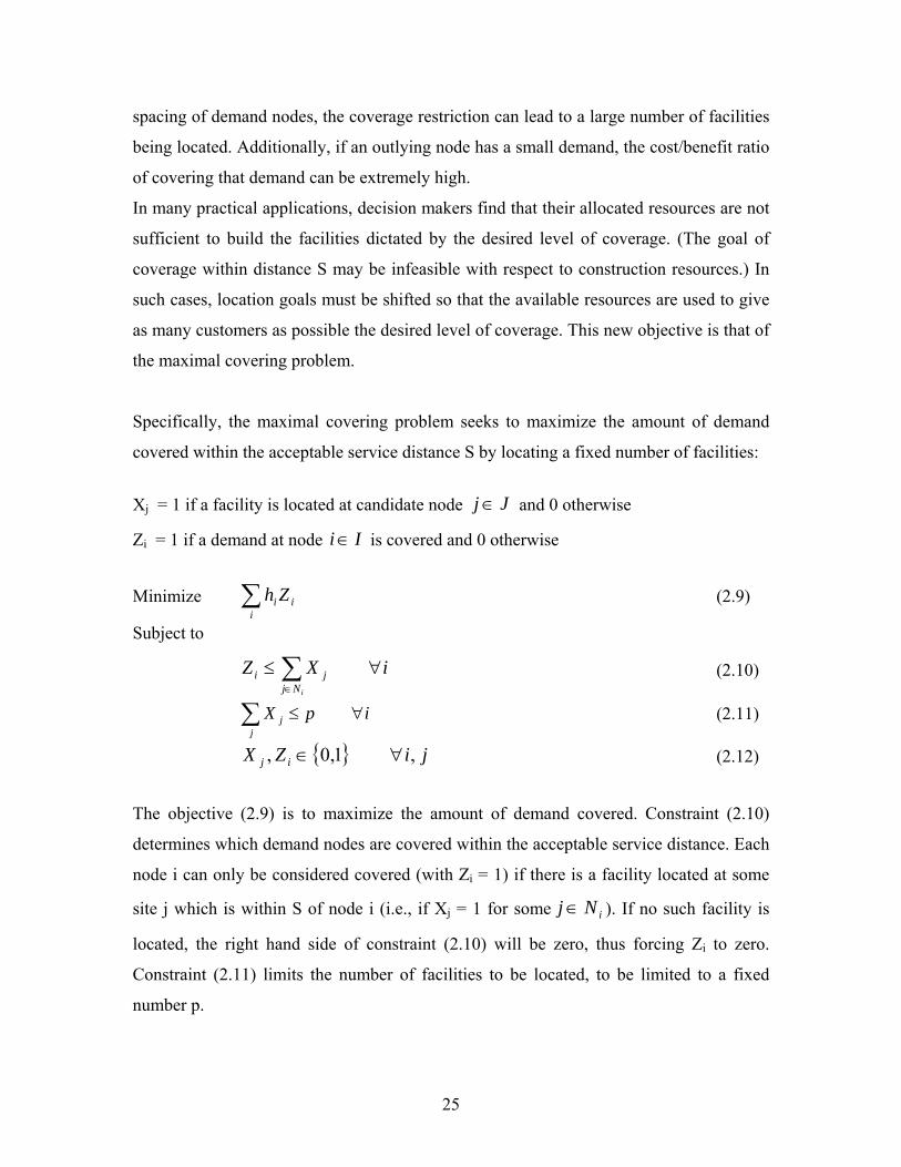
Specifically, the maximal covering problem seeks to maximize the amount of demand

covered within the acceptable service distance S by locating a fixed number of facilities:

Xj = 1 if a facility is located at candidate node Jj and 0 otherwise

Zi = 1 if a demand at node Ii is covered and 0 otherwise

Minimize i

ii Zh (2.9)

Subject to

iXZiNj

ji

(2.10)

ipXj

j (2.11)

jiZX ij ,1,0, (2.12)

The objective (2.9) is to maximize the amount of demand covered. Constraint (2.10)

determines which demand nodes are covered within the acceptable service distance. Each

node i can only be considered covered (with Zi = 1) if there is a facility located at some

site j which is within S of node i (i.e., if Xj = 1 for some iNj ). If no such facility is

located, the right hand side of constraint (2.10) will be zero, thus forcing Zi to zero.

Constraint (2.11) limits the number of facilities to be located, to be limited to a fixed

number p.

26

Center Problem

Another problem class which avoids the set covering problem's potential infeasibility is

the class of P-center problems. In such problems, we require coverage of all demands, but

we seek to locate a given number of facilities in such a way that minimizes coverage

distance. Rather than taking an input coverage distance S, this model determines

endogenously the minimal coverage distance associated with locating P facilities.

The P-center problem is also known as the minimax problem, as we seek to minimize the

maximum distance between any demand and its nearest facility. If facility locations are

restricted to the nodes of the network, the problem is a vertex center problem. Center

problems which allow facilities to be located anywhere on the network are absolute

center problems.

The following additional decision variable is needed in order to formulate the P-center

problem:

D = maximum distance between a demand node and the nearest facility.

The resulting integer programming formulation of the P-center problem follows.

Minimize D (2.13)

Subject to

ipXj

j (2.14)

iYj

ij 1 (2.15)

jiXY jij ,0 (2.16)

iDYdj

ijij (2.17)

jiYX ijj ,1,0, (2.18)

27

The objective function (2.13) is simply to minimize the maximum distance between any

demand node and its nearest facility. Constraints (2.14) limits the maximum number of

open facilities to p. constraints (2.15) enforces each demand point to be assigned to a

facility and constraints (2.16) make sure that demands are assigned only to selected

facilities. Constraint (2.17) defines the maximum distance between any demand node i

and the nearest facility j. Finally, constraints (2.18) are integrality constraints for the

decision variables.

In addition to three classes introduced here, several alternate formulations of the facility

location problem are proposed by researchers over the years. For a bibliography of recent

studies refer to ReVelle et al. (2008).

2.1.2. Vehicle Routing Problem

The vehicle routing problem (VRP) is a generic name given to a whole class of problems

in which a set of routes for a fleet of vehicles based at one or several depots must be

determined for a number of geographically dispersed cities or customers. The VRP arises

naturally as a central problem in the fields of transportation, distribution and logistics.

Usually, the objective of the VRP is to deliver a set of customers with known demands on

minimum-cost vehicle routes originating and terminating at a depot. In some market

sectors, transportation means a high percentage of the value added to goods. Therefore,

the utilization of modeling and optimization methods for transportation often results in

significant savings ranging from 5% to 20% in the total costs, as reported in Toth and

Vigo (2002).

The VRP is a well known integer programming problem which falls into the category of

NP-Hard problems, meaning that the computational effort required for solving this

problem increases exponentially with the problem size. This difficult combinatorial

problem conceptually lies at the intersection of these two well-studied NP-Hard

problems:

28

The Traveling Salesman Problem (TSP): If the capacity of the vehicles is infinite,

we can get an instance of the Multiple Traveling Salesman Problem (MTSP). An

MTSP instance can be transformed into an equivalent TSP instance by adding to

the graph k-1 (k being the number of routes) additional copies of node 0 and its

incident edges.

The Bin Packing Problem (BPP): The question of whether there exists a feasible

solution for a given instance of the VRP is an instance of the BPP. The decision

version of this problem is conceptually equivalent to a VRP model in which all

edge costs are taken to be zero (so that all feasible solutions have the same cost).

Three basic approaches have been proposed for modeling VRP in the literature (Toth and

Vigo 2002). The models of the first type, known as Vehicle Flow formulation, use binary

integer variables associated with each arc of the network, which shows if an specific arc

is traverse by a vehicle or not. These models are often used for basic versions of VRP.

They are particularly useful for cases in which the cost of the solution can be expressed

as the sum of the costs associated with the arcs. On the other hand, vehicle flow models

cannot be used to deal with many practical issues; for instance, when the cost of a

solution depends on the sequence of traversed arcs or when the cost depends on the type

of vehicle that is assigned to a route.

The second approach to VRP modeling is called Commodity Flow formulation. In this

type of model, additional integer variables are associated with arcs that represent the flow

of the commodities along the paths traveled by the vehicles. In some recent studies, these

models have been used as a basis to solve for the exact solutions of capacitated VRP.

In the third approach to VRP modeling, the decision variables are the feasible routes for

the vehicles. These models produce an exponential number of binary variables each

associated with a feasible route. Then the VRP is formulated as a Set Partitioning

problem that tries to select a set of routes with minimum cost which serves each costumer

once and also satisfies the additional constraints. Main advantage of this type of model is

29

that it allows for extremely general route costs. For example, route costs can be nonlinear

or can depend on the vehicle type or sequence of nodes visited. Also, the linear relaxation

of these models usually provides a tighter bound than the previous models. However,

these models usually require enumerating the feasible routes which needs extensive

preprocessing and results in a very large number of variables.

Mathematical Formulation

As mentioned above, vehicle flow based formulation is one of the approaches to model

the VRP. Following formulation is an example for the base case of uncapacitated multi-

vehicle single depot vehicle routing problem. The decision variables vijx which are binary

indicate whether vehicle v travels from point i to point j, vijx =1, or not v

ijx =0

Minimize i j v

vijij xc (2.19)

Subject to

jxv i

vij 1 (2.20)

ixv j

vij 1 (2.21)

vNpxxj

vpj

i

vip ,0 (2.22)

vxj

vj 10 (2.23)

vjixvij ,,1,0 (2.24)

SX (2.25)

The objective is to minimize the total travel cost (or distance) by all vehicles. Constraints

(2.20) through (2.22) require that only one vehicle enters each node and that the same

vehicle exits that node. Constraints (2.23) insure that each vehicle leaves the depot only

once. The last condition which is imposed on the matrix X prohibits subtours that do not

contain the depot. There are several possible ways to fulfill this condition, for example S

30

might be composed of subtour breaking constraints for each vehicle. S can be defined as

the union of sets Sv defined by:

Qi Qj

vij

vijv QsubsetnonemptyallforQxxS 1: (2.26)

If each customer has a demand of di units and each vehicle has a capacity of Kv, then the

capacitated VRP can be formulated by adding the following capacity constraints to the

base formulation:

vKxd vi j

viji

(2.27)

VRP Variants

Usually, real world vehicle routing problems are much more sophisticated than the base

case VRP introduced above. Over the years, researchers have proposed variants of VRP

by adding some constraints to the base case VRP formulation. Here, a list of well-known

VRP variants is summarized:

Capacitated VRP (CVRP): Every vehicle has a limited capacity

Distance-Constrained VRP (DCVRP): The maximum tour length is limited

Multiple Depot VRP (MDVRP): The vendor uses many depots to supply the

customers

VRP with Pick-Up and Delivering (VRPPD): Customers may return some goods

to the depot

Split Delivery VRP (SDVRP): The customers may be served by different vehicles

VRP with time windows (VRPTW): Every customer has to be supplied within a

certain time window

Periodic VRP (PVRP): The deliveries may be done in some consecutive days

Stochastic VRP (SVRP): Some values, such as number of customers, theirs

demands, service time or travel time, are random

31

There are several survey papers on the VRP, VRP variants, and their solution algorithms

and techniques. A classification of the problem was given in Desrochers et al.(1990).

Laporte and Nobert (1987) presented a survey of exact methods to solve VRP. Other

surveys that provided exact and heuristic methods were presented by Christofides,

Mingozzi, and Toth (1981), Magnanti (1981), Bodin et al.(1983), Fisher (1994), Laporte

(1992), Toth and Vigo (2002). An annotated bibliography was proposed by Laporte

(1997). A book on the subject was edited by Golden and Assad (1988).

2.2. Commercial Supply Chain versus Emergency Response Logistics

Immediately after the disaster, humanitarian organizations often face significant problems

of transporting large amounts of many different commodities including food, clothing,

medicine, medical supplies, machinery, and personnel from several origins to several

destinations inside the disaster area. The transportation of supplies and relief personnel

must be done quickly and efficiently to maximize the survival rate of the affected

population and minimize the cost of such operations.

When it comes to efficiency of supply deliveries, the modeling and optimization

techniques established in commercial supply chain management seem to be the most

relevant approach. For instance, some of the quickest emergency assistance to the victims

of hurricane Katrina did not come from the American Red Cross or FEMA, it came from

Wal-Mart. Millions of affected or displaced people waited for days as agencies struggled

to provide assistance. Wal-Mart moved faster than traditional emergency aid groups

mainly because the retail giant had mastered the fundamentals of logistics and supply

chain management (Dimitruk 2005).

More recently, some studies such as (Beamon 2004; Thomas and Kopczak, 2005; Van

Wassenhove, 2006; Oloruntoba and Gray, 2006; Thomas, 2007), emphasized that some

32

supply chain concepts share similarities to emergency logistics and therefore some tools

and methods developed for commercial supply chains can be successfully adapted in

emergency response logistics.

Using commercial supply chain techniques in disaster management is still in its infancy.

Beamon (2004) and Thomas (2005) have compared the current state of supply chain

management capabilities within humanitarian organizations with that of the commercial

sector in the 1970s and 1980s. At that time, the commercial sector just began to realize

the strategic advantages and significant improvements supply chain management could

offer in effectiveness and efficiency. This led to extensive research in the area of supply

chain and logistical analysis but those quantitative methods and principles are rarely

applied to humanitarian operations on the verge of disasters.

The partial reason is the difference in the strategic goals of commercial supply chain with

goals of disaster response logistics. The main goal in commercial supply chain is to

minimize the cost or maximize the profit of operations. Actions are justified if they

increase the profit but are not perused if their cost is more than their profit. However,

humanitarian organizations are mostly non-profit organizations with the idea of providing

critical services to the public in order to minimize the pain and sufferings, for example

after a natural disaster.

One major difference between the two types of chains is the demand pattern. For many

commercial supply chains, the external demand for products is comparatively stable and

predictable. Often, for the commercial chain, the demands seen from warehouses occur

from established locations in relatively regular intervals. However, the demands in the

relief chain are emergency items, equipment, and personnel. More importantly, those

demands occur in irregular amounts and at irregular intervals and occur suddenly, such

that the locations are often completely unknown until the demand occurs.

Beamon (2004) suggests other specific characteristics of disaster response logistics that

differentiate them from traditional commercial supply chains. These include

33

Zero lead time that dramatically affects inventory availability, procurement, and

distribution.

High stakes (often life-and-death) that requires speed and efficiency

Unreliable, incomplete, or non-existent supply and transportation infrastructure.

Many relief operations are naturally ad hoc, without effective monitoring and

control.

Variable levels of technology is available depending on the disaster area

Table 2.1 compares some of the differences between commercial and humanitarian

supply chains.

Table 2.1- Commercial Supply Chains vs. Humanitarian Relief Chains (Beamon 2004)

Characteristic Commercial Chain Humanitarian Relief Chain

Strategic Goals

Typically to produce high quality

products at low cost to maximize

profitability

Minimize loss of life and alleviate

suffering.

Distribution

Network

Configuration

Well-defined methods for

determining the number and

locations of distribution centers.

Challenging due to the nature of the

unknowns (locations, type and size of

events, politics, and culture)

What is

“Demand”? Products.

Emergency Supplies, equipment and

Personnel.

Lead Time Lead time determined by the

supplier-manufacturer-DC-retailer

Zero time between the occurrence of the

demand and the need for the demand

Inventory Control

Utilizes well-defined methods for

determining inventory levels

based on lead time, demand and

target customer service levels.

Inventory control is challenging due to the

high variations in lead times, demands,

and demand locations.

Information

System

Generally well-defined, using

advanced technology.

Information is often unreliable,

incomplete or non-existent.

34

It is concluded that some of the concepts associated with commercial supply chains are

directly applicable to humanitarian relief chains. However, future work must develop

methods that specifically address the challenges presented by characteristics unique to

humanitarian relief and logistics of disaster response.

2.3. Logistics in Disaster Response

Altay and Green (2006) surveyed the existing literature of emergency disaster

management. They concluded that most of the disaster management research was related

to social sciences and humanities literature. (Refer to Hughes (1991) and

http://www.geo.umass.edu/courses/geo510/index.htm for a comprehensive bibliography)

That type of research focuses on subjects such as disaster results, sociological impacts on

communities, psychological effects on survivors or rescue teams, and organizational

design and communication problems. They observed that the existing literature is

relatively light on disaster management articles that used operations research or

management science (OR/MS) techniques to deal with the problem. However, they

realized the literature trend that more studies are focusing on OR/MS techniques in recent

years and emphasized the need for more research in future.

In the following sections, a summery of studies is presented that use OR/MS techniques

to model and optimize the emergency disaster management activities. This is not an

exclusive list of publication in the field and is only intended to focus on key studies in the

past that successfully used techniques that are relevant to the subject of this dissertation.

2.3.1 Early Ages

A number of authors have recognized the problem of emergency response management in

its early ages. Kemball-Cook and Stephenson (1984) addressed the need for logistics

management in relief operations for the increasing refugee population in Somalia.

Ardekani and Hobeika (1988) addressed the need of logistics management in relief

35

operations for the 1985 Mexico City earthquake. Knott (1987) developed a linear

programming model for the bulk food transportation problem and the efficient use of the

truck fleet to minimize the transportation cost or to maximize the amount of food

delivered (single commodity, single modal network flow problem). In another article,

Knott (1988) developed a linear programming model using expert knowledge for the

vehicle scheduling of bulk relief of food to a disaster area.

Ray (1987) developed a single-commodity, multi-modal network flow model on a

capacitated network over a multi-period planning horizon to minimize the sum of all

costs incurred during the transport and storage of food aid. Brown and Vassiliou (1993)

developed a real-time decision support system which uses optimization methods,

simulation, and the decision maker’s judgment for operational assignment of units to

tasks and for tactical allocation of units to task requirements in repairing major damage to

public works following a disaster.

The literature in the multi-commodity, multi-modal network flow problem was relatively

sparse. Crainic and Rousseau (1986) developed an optimization algorithm based on

decomposition and column generation principles to minimize the total operating and

delay cost for multi-commodity, multi-modal freight transportation when a single

organization controls both the service network and the transportation of goods. Guelat et

al. (1990) presented a multi-commodity, multi-modal network assignment model for the

purpose of strategic planning to predict multi-commodity flows over a multi-modal

network. The objective function to be minimized was the sum of total routing cost and

total transfer cost.

2.3.2 Recent Studies

Technology advancement in resent years opened new doors for researchers. Haghani and

Oh (1996) proposed a formulation and solution of a multi-commodity, multi-modal

network flow model for disaster relief operations. Their model can determine detailed

36

routing and scheduling plans for multiple transportation modes carrying various relief

commodities from multiple supply points to demand points in the disaster area. They

formulated the multi-depot mixed pickup and delivery vehicle routing problem with time

windows as a special network flow problem over a time-space network. The objective

was minimizing the sum of the vehicular flow costs, commodity flow costs,

supply/demand storage costs and inter-modal transfer costs over all time periods. They

developed two heuristic solution algorithms; the first was a Lagrangian relaxation

approach, and the second was an iterative fix-and-run process. Their work is one of the

few that can be implemented at operational level.

Barbarosoglu et al. (2002) focused on tactical and operational scheduling of helicopter

activities in a disaster relief operation. They proposed a bi-level modeling framework to

address the crew assignment, routing and transportation issues during the initial response

phase of disaster management in a static manner. The top level mainly involves tactical

decisions of determining the helicopter fleet, pilot assignments and the total number of

tours to be performed by each helicopter without explicitly considering the detailed

routing of the helicopters among disaster nodes. The base level addresses operational

decisions such as the vehicle routing of helicopters from the operation base to disaster

points in the emergency area, the load/unload, delivery, transshipment and rescue plans

of each helicopter in each tour, and the re-fueling schedule of each helicopter given the

solution of the top level.

Barbarosoglu and Arda (2004) developed a two-stage stochastic programming model for

transportation planning in disaster response. Their study expanded on the deterministic

multi-commodity, multi-modal network flow problem of Haghani and Oh (1996) by

including uncertainties in supply, route capacities, and demand requirements. The authors

designed 8 earthquake scenarios to test their approach on real-world problem instances. It

is a planning model that does not deal with the important details that might be required at

strategic or operational level. It does not address facility location problem or vehicle

routing problem.

37

Ozdamar et al. (2004) addressed an emergency logistics problem for distributing multiple

commodities from a number of supply centers to distribution centers near the affected

areas. They formulated a multi-period multi-commodity network flow model to

determine pick up and delivery schedules for vehicles as well as the quantities of loads

delivered on these routes, with the objective of minimizing the amount of unsatisfied

demand over time. The structure of the proposed formulation enabled them to regenerate

plans based on changing demand, supply quantities, and fleet size. They developed an

iterative Lagrangian relaxation algorithm and a greedy heuristic to solve the problem.

Yi and Ozdamar (2007) proposed a model that integrated the supply delivery with

evacuation of wounded people in disaster response activities. They considered

establishment of temporary emergency facilities in disaster area to serve the medical

needs of victims immediately after disaster. They used the capacity of vehicles to move

wounded people as well as relief commodities. Their model considered vehicle routing

problem in conjunction with facility location problem. The proposed model is a mixed

integer multi-commodity network flow model that treats vehicles as integer commodity

flows rather than binary variables. That resulted in a more compact formulation but post

processing was needed to extract detailed vehicle routing and pick up or delivery

schedule. They reported that post processing algorithm was pseudo-polynomial in terms

of the number of vehicles utilized.

In a recent study, Balcik and Beamon (2008) proposed a model to determine the number

and locations of distribution centers to be uses in relief operations. They formulated the

location finding problem as a variant of maximum covering problem when the demand

estimations are available for a set of likely scenarios. Their objective function maximizes

the total expected demand covered by the established distribution centers. They also

solve for the amount of relief supplies to be stocked at each distribution center to meet

the demands. Their study is one of the first to solve location finding problem in relief

operation; however, they do not consider the location problem as part of a supply chain

network. Consequently, they cannot consider the interactions between optimal

38

transportation of relief items from sources to the demand points and problem of finding

optimal locations for distribution facilities.

2.4. Conclusions

There are not many publications that directly applied network modeling and optimization

techniques in disaster response. Among those studies, there is no model that has

integrated the interrelated problems of large scale multicommodity multimodal network

flow problem, vehicle routing problem with split mixed pick up and delivery, and optimal

location finding problem with multiple layers. Also to the best of our knowledge, there is

no mathematical model that describes the special structure of FEMA’s supply chain

system.

It is intended to fill some of these gaps in the following sections of this research. After

providing a more formal description of the problem, a mathematical model is proposed

that considers the specific characteristics of the described problem. The proposed

mathematical model is a comprehensive system that integrates all the abovementioned

properties. Offering this large-scale mathematical formulation is a theoretical

contribution by itself. Nevertheless, solving this large-scale integrated formulation for

real-world size problems requires special considerations.

The problem belongs to the NP-Hard class that is proven to be extremely time consuming

as the problem size grows. Offering efficient solution algorithms and heuristics is another

gap that is being investigated in this research. Extensive numerical and sensitivity

analysis are required to evaluate the different aspects of the model and solution

algorithms. Through case studies and simulation scenarios, it will be possible to compare

the integrated model with sequential models. In this research, it is intended to investigate

the possible advantages of using integrated model compared to solving the problem

sequentially and report the results. Such comparison does not exist in current literature to

the best of the author’s knowledge.

39

Chapter 3: Problem Description and Formulation

In this section, first a complete description of the problem and its properties are provided.

Then the research approach to model the problem is described followed by the list of

assumption made in order to properly model the problem. Finally, the details of

mathematical formulation for the proposed model are presented in section 3.4. The

parameters and variables are defined first, then the objective function of the optimization

problem is introduced in section 3.4.4 followed by the formulation and description of the

constraints of the problem. Finally, in section 3.5, a short form of the mathematical

formulation is presented for the summary.

3.1. Problem Description

The goal is to orchestrate all the components and tasks in the emergency response

operations after a large scale disaster, in order to minimize the loss of life or human

sufferings by rapid and efficient delivery of critical relief items to the victims in the

disaster areas.

Logistics planning in emergencies involves sending multiple relief commodities (e.g.,

medicine, water, food, equipment, etc) from a number of sources to several distribution

points in the affected areas through a chain structure with some intermediate transfer

nodes. The supplies may not be available immediately but arrive over time. It is a

difficult task to decide on the right type and quantity of relief items, the sources and

destinations of commodities, and also how to dispatch relief items to the recipients in

order to minimize the pain and sufferings for the disaster victims.

It is necessary to have a quick estimation of the demands during the initial response time.

It is essential to know the types of required commodities, the amount of each commodity

per person or household, an estimation of the number of victims, and the geographical

locations of the demands. The list of commodities includes but is not limited to water,

40

food, shelter, electric generators, medical supplies, cots, blankets, tarps and clothing.

Some of the demand items are one-time demand while others are recurring (e.g. tent vs.

water) and some demands are subject to expiration while others may be carried over (e.g.

food vs. clothing). The demand usually overwhelms the capacity of the distribution

network. The demand information might not be complete and accurate at the beginning

but it is expected to improve over time.

Different aid organizations may employ their unique supply chain structure that governs

the types of facilities to be used and the relationships among components of the chain.

For example FEMA has its own supply chain structure for disaster response which is

previously introduced in section 1.4. FEMA has distinguished 7 layers of facilities in its

logistics chain. First 3 layers are permanent facilities to store and ship the relief items

while the next 4 layers are temporary transfer facilities that their numbers and locations

will be chosen during the response phase.

During the initial response time it is also necessary to set up temporary transfer facilities

to receive, arrange, and ship the relief commodities through the distribution network. In

risk mitigation studies for disasters, possible sites where these facilities can be situated

are specified. Logistics coordination in disasters involves the selection of sites that result

in the maximum coverage of affected areas and the minimum delays for supply delivery

operations. Usually the number of these temporary facilities is limited because of the

equipment and personnel constraints.

Each facility in the chain is subject to some capacity constraints. Capacities are defined

for operations such as sending, receiving, and storing commodities. These capacities are

different for each facility and are determined based on the type, size and layout of that

facility. Also the availability of personnel and equipment may influence the capacities. In

general, the capacity constraints can be defined in terms of the weight or volume of the

commodities or they can be defined in terms of the numbers of the vehicles that are sent,

received, or parked at the facility at a certain time. These are two different aspects and it

is recommended to consider both capacities for each facility.

41

The transportation capacity is usually very limited in early hours or days after a disaster.

It is very critical to assign the available fleet to the best possible use at any time. There is

usually a shortage of vehicles in emergency operations so the model must keep track of the empty

trucks in order to assign them to new missions after each delivery. More than one

transportation mode may be hired to facilitate emergency response logistics.

Consequently, the coordination and cooperation between transportation modes are

necessary for managing the response operations and providing a seamless flow of relief

commodities toward the aid recipients. The intermodal transfer of commodities is

expected to happen in specific facilities but may be subject to some capacity constraints

and transfer delays.

Vehicle routing and scheduling during the disaster response is also very important. A

large number of vehicles might be used in response to large scale disasters. The model

should be able to keep track of routings for each individual vehicle. Also, it is required to

have a detailed schedule for pick up and delivery of relief commodities by each vehicle in

each transportation mode. Nonetheless, the vehicle routing in disaster situations are quite

different from conventional vehicle routings. The vehicles do not need to form a tour and

return to the assigned depot, but they might be assigned to a new path at any time. They

are expected to perform mixed pickup and delivery of multiple items between different

nodes of the network as the supplies and demands arise over time.

The disaster area is a dynamic environment and emergency logistics are very time

sensitive operations. The disaster might still be evolving when the response operations

start. Also the lack of vital information about available infrastructure, supplies, and

demands in the initial periods after the disaster may complicate this dynamic environment

even more. The high stake of life-or-death for disaster victims urges the needs for higher

levels of accuracy and tractability. Despite all the necessary preparedness and planning at

strategic level, dealing with the problem as operational level is very important. Modeling

and optimization at operation level is the only approach to capture the realities of the time

sensitive emergency response operations.

42

The other important issue is considering equity and fairness among aid recipients. Based

on the geographical dispersion of victims and availability of resources over time and

space, it is easy to favor the demands of one group of victims over another. Even though

some variations are inevitable, the ideal pattern is to distribute the help items evenly and

fairly among the victims. The models and procedures with general objective functions are

prone to ignore the equity and level of service requirements in order to get a better

numerical solution. It is very important to realize the need for procedures and constraints

that prevent any sort of discrimination among victims, as much as possible.

The equity constraint between populations can be defined over time, and over

commodities. It is not appropriate to satisfy all the demands of one group in early stages

while the other group of victims does not receive any help until very later times. It is

more acceptable to fairly distribute the available relief items among all recipients even

though it might not be enough for every one at the current instance. The relief operations

will continue over time as more resources are expected to become available. The equity

over commodities is also important. For example, it is not acceptable to send all the

available water to one group of victims and send all the available meals to another group.

It is expected to fairly share the limited resources of transportation capacity and disaster

relief commodities.

3.2. Time-Space Network

A physical network is converted into a time-space network to account for the dynamic

decision process. In the context of the problem of this research, nodes in the time-space

network represent the physical locations of the supply and demand points for each mode

and over time, while the arcs represent the connecting routes between these points. Each

node in the physical network is represented by the number of mode types at each time

period of the planning horizon. In a sense the time-space network in this context can be

thought of as an overlay of several physical networks, one for each mode, which are

represented over time. These overlaid networks are connected to each other by the

43

transfer links which make it possible for the commodities to be transferred between

modes.

There are three types of traffic flow on the physical network. The first type is the routing

traffic that moves from one node to another node by a certain type of mode. The second

type is the transfer traffic that changes mode type from one mode to another mode at a

certain node. The third type is the supply or demand carry-over that is carried over to the

next time period at a certain node.

The duration of one time period should be based on the link travel time for each mode. It

must be small enough so that the amount of slack time on the routing links is not

excessive. However, the planning horizon should not be too short in order for the time-

space network to be meaningful. Also, it should not be too long as it will increase the

dimension of the time-space network and make the problem difficult to solve.

The movements of commodities and personnel on a physical network over time are

represented by the links in the time-space network. Routing Links represent the physical

movement of commodities in space. Transfer Links represent the transfer of traffic

between the available modes. Finally, Supply or Demand Carry-Over Links represent the

commodity supply or demand carry over from one period to the next.

Figure 3.1 shows a physical network that has 4 nodes, 5 two-way arcs, and 2 modes.

Node A represents the origin and nodes C and D denote the destinations. The travel time

over the arc in each mode type is shown in terms of time periods. Figure 3.2 shows the

time-space network generated from Figure 3.1 with 6 time units of planning horizon. The

length of one time period is assumed to be one time unit. In Figure 3.2, all transfer time is

assumed to be one time period. The carry-over links that are created at node A and B

represent the supply carry-over links. On the other hand, the carry-over links that are

shown at node C and D denote the demand carry-over links.

44

Figure 3.1. Physical Network

Figure 3.2. Time-Space Network

Mode M

Time period 0 1 2 3 4 5 6

Routing Flow Transfer Flow Carry-over Flow

A

B

C

D

A

B

C

D

Mode N

A

C

B

D

(1,2)

(1,2)

(2,4)

(2,3)

(1,2)

Origin Destination

Destination

Transfer

45

3.3. Modeling Approach

A mathematical framework is suggested to model the supply chain operations during

emergency response, as the problem is described in section 3.1. The main characteristics

of the modeling approach can be summarized as follow:

Operational Level: to capture time sensitive details of the emergency response

operations, the problem is formulated at operational level.

FEMA Structure: the proposed model is in compliance with FEMA’s 7-layer supply

chain structure.

Time-Space Network: to account for the dynamic decision process, the physical

network must be converted to a time-space network. The nodes of this network

represent the facilities in FEMA structure. The links consist of existing physical links,

delay or storage links, and intermodal transfer links.

Facility Location: the optimal locations to establish temporary facilities are selected

from a set of potential sites. The maximum number of each facility type and their

locations are dynamic and can change over time as the relief operations proceed.

Facility Capacity: each facility has maximum capacities for sending, receiving, and

storing commodities as well as vehicles.

Demand: the demand is multi-commodity and usually overwhelms the capacity of

the distribution network. Specific decision variables are defined that keep track of

unsatisfied demand at each demand point for each commodity and during all time

periods.

Supply: similar to the demand, the supply is multi-commodity and may come from

various sources. The problem is formulated as a variation of multi-commodity

network flow problem.

Multi Modal: since more than one mode of transportation may be hired in the

emergency response logistics, the problem is a variation of multi-modal network flow

problem.

46

Vehicle Routing: in order to model the complicated routing and delivery operations

in disaster response, the vehicles are treated as flow of integer commodities over the

time-space network. This results in a mixed integer multi-commodity formulation.

Network Capacity: a set of constraints is used to link the relief commodities with the

vehicles. As a result, the flow of commodities is only possible when accompanied by

enough vehicle capacity for that specific link and time.

Integrated Model: all decisions of facility location, supply delivery, and vehicle

routing, are interrelated. Our approach provides an integrated model to find the global

solution for this problem.

Equity: equity and fairness among disaster victims is modeled through a set of

constraints that enforce a minimum level-of-service for each victim. The equity is

required for each relief item and over all time periods.

Objective Function: the objective of this model is to minimize the pain and suffering

of the disaster victims. It is formulated as total of unsatisfied demand summarized for

all victims, for all relief items, and during all time periods.

3.4 Assumptions

1- It is assumed that the following information is given:

Demands: types, locations, amounts

Supply: types, locations, amounts

Permanent Facilities: types, locations, capacities

Temporary Facilities: set of potential sites for each type, capacities of each

type

Network: link-node incidence matrix for each transportation mode

Vehicles: number available for each mode and their initial location, capacity

of each vehicle

Travel Times: travel time on each link for each transportation mode.

47

2- Because the model is at the operational level, it is assumed that the problem is

deterministic. The required information is estimated or known at the beginning of the

operations. The model can adapt to the required information as it evolves over time.

3- Supply Chain Structure:

It is assumed that the flow of commodities between each two node is possible

only if it is in compliance with FEMA’s structure shown in Figure 1.5. For

example, the supply from LC can not be sent directly to SSA. It should be

sent to MOBs or FOSAs first.

It is assumed that for the empty vehicles, a direct link exists that connects

each pair of nodes. For example, if a vehicle delivers all of its supply at a

POD, it can directly go to any other node of the network to pick up new

supplies.

4- Finding the number and location of Points of Distribution (PODs) is not considered in

this study. It is assumed that PODs are established by local authorities. As a result, the

location and amount of demands at each POD is a given data for this model.

3.5. Mathematical model

In this section initially the notations and required parameters for the formulation are

introduced. After that, the decision variables of the mathematical model are defined.

Then the objective function formulation is presented followed by formulation and

introduction of the constraints of the problem.

3.5.1 Notations

N = Set of all nodes. Nji , are indices

LC = Set of Logistic Center sites

CSS = Set of Commercial Storage Sites

VEN = Set of commodity Vendor sites

MOB = Set of potential sites for Mobilization Centers

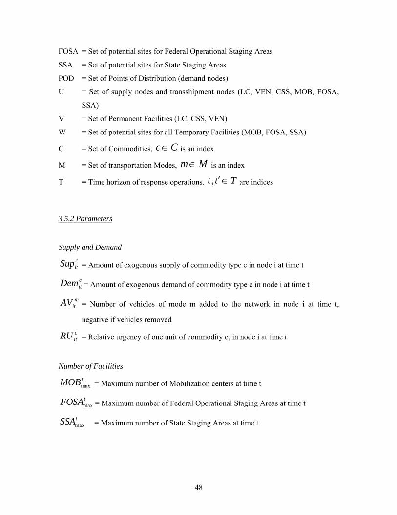
48

FOSA = Set of potential sites for Federal Operational Staging Areas

SSA = Set of potential sites for State Staging Areas

POD = Set of Points of Distribution (demand nodes)

U = Set of supply nodes and transshipment nodes (LC, VEN, CSS, MOB, FOSA,

SSA)

V = Set of Permanent Facilities (LC, CSS, VEN)

W = Set of potential sites for all Temporary Facilities (MOB, FOSA, SSA)

C = Set of Commodities, Cc is an index

M = Set of transportation Modes, Mm is an index

T = Time horizon of response operations. Ttt , are indices

3.5.2 Parameters

Supply and Demand

citSup = Amount of exogenous supply of commodity type c in node i at time t

citDem = Amount of exogenous demand of commodity type c in node i at time t

mitAV = Number of vehicles of mode m added to the network in node i at time t,

negative if vehicles removed

citRU = Relative urgency of one unit of commodity c, in node i at time t

Number of Facilities

tMOBmax = Maximum number of Mobilization centers at time t

tFOSAmax = Maximum number of Federal Operational Staging Areas at time t

tSSAmax = Maximum number of State Staging Areas at time t

49

Facility Capacity

mitUcap = Unloading capacity for the facility in node i for mode m at time t

itScap = Storage capacity for the facility in node i at time t

mitLcap = Loading capacity for the facility in node i for mode m at time t

mitVRcap = Maximum number of mode m vehicles that can be received at the facility in

node i at time t

mitVPcap = Maximum number of mode m vehicles that can be parked (carried over) at

the facility in node i from time t to time t + 1

mitVScap = Maximum number of mode m vehicles that can be sent out from the facility

in node i at time t

Vehicle Capacity

mcap = Loading capacity of vehicles of mode m

cw = Unit weight of commodity c

Transportation

ijmt = Travel time from node i to node j for vehicles of mode m

mmK = Time required to transfer commodities from mode m to mode m

3.5.3 Decision Variables

Location Problem

tiLoc = 1 if temporary facility of appropriate type is located at potential site i, at time t;

equal to 0 otherwise. The temporary facility will be a Mobilization Center if

50

MOBi , a Federal Operational Staging Area if FOSAi , and a State

Staging Area if SSAi .

Commodity and Vehicle Flow

cmijtX = Flow of commodity type c shipped from node i to node j by mode m at time t

mijtY = Flow of vehicles of mode m from node i to node j at time t

citCX = Amount of commodity type c in node i which is carried over from time period t

to t + 1

mitCY = Number of vehicles of mode m in node i which is carried over from time period

t to t + 1

mcmitXT

= Amount of commodity type c in node i which is transferred from mode m to

mode m′ at time t

citUD = Amount of unsatisfied demand of commodity type c in node i at time t

3.5.4 Objective Function

Minimize

Vi t c

cit

cit UDRU (3.1)

The objective function in equation (3.1) minimizes the total amount of weighted

unsatisfied demand over all commodities, times, and demand points. citRU is the relative

urgency associated with each commodity, time, and demand point. If there is any desire

to consider a commodity being more important than others at any time or for any demand

point, citRU can enforce that desire. Higher value of

citRU translates into higher

urgencies. If all the commodities happen to be of the same importance, citRU can be set

equal to 1.

51

3.5.5 Constraints

Commodity Flow Constraints

Supply nodes and Transfer nodes:

tmcUiCXXTX

SupCXXTX

cit

m

mmit

j

cmijt

cit

cti

m

mmckti

j

cmttji mmjim

,,,

)1()()(

(3.2)

Demand nodes:

tcPODiUDDemUDX cti

cit

cit

m j

cmttji jim

,,)1()( (3.3)

Equations (3.2) and (3.3) enforce the conservation of the flow for all commodities and

modes at all nodes and time periods. Equation (3.2) requires that for supply nodes and

transfer nodes, the sum of the flows entering each node plus exogenous supply should be

equal to the sum of the flows that leave the same node. Equation (3.3) shows that the total

flow entering each demand node plus the unsatisfied demand is equal to the exogenous

demand at that node plus the unsatisfied demand from the previous time period.

Vehicular Flow Constraints

tmNiCYYAVCYY mit

j

mijt

mit

mti

j

mttji jim

,,)1()( (3.4)

Equation (3.4) represents the conservation of flow for the vehicles. At any node i and

time period t, total number of available vehicles of mode m is equal to the number of

vehicles of mode m that left node j for node i at time ijmtt , plus the number of

vehicles that were carried over from the previous time period, plus the number of

vehicles that are added or removed to the fleet at that time. These vehicles are either sent

out of the node or carried over to the next time period.

52

Linkage between Commodities and Vehicles

tmNiXwYCapc

cmijtc

mijtm ,, (3.5)

Constraint (3.5) makes sure that commodities are not sent out of a node unless a number

of vehicles with enough capacity are available at that node.

Facility Capacities for Permanent Facilities

tmViLcapX mit

c j

cmijt ,, (3.6)

tmLCiUcapX mit

c j

cmttji jim

,,)( (3.7)

tmViScapSupCX

XTX

itc

cit

c

cti

c m m

mmckti

m c j

cmttji mmjim

,,)1(

)()(

(3.8)

tmViVScapY mit

j

mijt ,, (3.9)

tmViVRcapAVY mit

mit

j

mttji jim

,,)( (3.10)

tmViVPcapCYAVY mit

mti

mit

j

mttji jim

,,)1()( (3.11)

Equations (3.6), (3.7), and (3.8) are the maximum capacity for loading, unloading, and

storage of commodities at permanent facilities. Equations (3.9), (3.10), and (3.11) require

the maximum number of vehicles that are sent, received, and parked at each facility to be

less than the relevant capacities.

Facility Location and Capacities for Temporary Facilities

tmWiLocLcapX ti

mit

c j

cmijt ,, (3.12)

53

tmWiLocUcapX ti

mit

c j

cmttji jim

,,)( (3.13)

tWiLocScapSupCX

XTX

tiit

c

cit

c

cti

c m m

mmckti

m c j

cmttji mmjim

,)1(

)()(

(3.14)

tmWiLocVRcapAVY ti

mit

mit

j

mttji jim

,,)( (3.15)

tmWiLocVPcapCYAVY ti

mit

mti

mit

j

mttji jim

,,)1()( (3.16)

tmWiLocVScapY ti

mit

j

mijt ,, (3.17)

tMOBiMOBLoc t

i

ti ,max (3.18)

tFOSAiFOSALoc t

i

ti ,max (3.19)

tSSAiSSALoc t

i

ti ,max (3.20)

Equations (3.12) through (3.14) enforce the loading, unloading, and storage capacity for

the temporary facilities. If the facility is selected to be set up at potential site i, the

respected capacity constraint is enforced. If it is decided not to set up the temporary

facility at location i, the same constraints require that all the flows in and out of that node

to be equal to zero.

Equations (3.15) through (3.17) require the maximum number of vehicles that are sent,

received, and parked at each temporary facility to be less than the relevant capacities. The

numbers are zero if the facility is not selected for that node.

Equations (3.18) through (3.20) oblige the maximum number of each temporary facility

type to be limited by the maximum allowable numbers for that facility type during the

chosen time periods.

54

Capacities for PODs:

tmPODiUcapX mit

c j

cmttji jim

,,)( (3.21)

tmPODiVRcapY mit

j

mttji jim

,,)( (3.22)

tmPODiVPcapCYY mit

mti

j

mttji jim

,,)1()( (3.23)

Equation (3.21) enforces the commodity unloading capacity at points of distribution.

Equation (3.22) and (3.23) represent the vehicle receiving and vehicle parking capacities

for each point of distribution.

Equity Constraint:

tcPODiDem

X

t

cti

t m j

cmttji jim

,,min

)(

(3.24)

tcPODiX

X

c t m j

cmttji

t m j

cmttji

jim

jim

,,min)(

)(

(3.25)

tPODiX

X

i c t m j

cmttji

c t m j

cmttji

jim

jim

,min)(

)(

(3.26)

Equation (3.24) enforces a minimum percentage of total demand for a specific

commodity c, to be satisfied by the time period t. It might not be always possible to

deliver the required amount by time t; in that case, this constraint makes the optimization

problem infeasible.

55

Equation (3.25) requires that from all commodities being delivered to node i by time t, at

least min percent to be commodity c.

Equation (3.26) ensures that sum of total commodities delivered at point i to be more than

a minimum percentage of all the commodities that are being delivered among all demand

points.

Nonnegativity and Integrality:

cmijtX ,

citCX ,

mcmitXT

, 0citUD Real-valued variables

mijtY , 0m

itCY General integer variables

)1,0(tiLOC Binary integer variables

3.6. Summary

The proposed mathematical model in this chapter can be summarized as follows:

Minimize Total Unsatisfied Weighted Demand

Subject to:

Commodity Flow Constraints

Vehicular Flow Constraints

Constraints that Link Commodities and Vehicles

Facilities Location Constraints

Facility Capacities Constraints

Equity (recipients/commodities) Constraints

Nonnegativity and Integrality Constraints

56

Chapter 4: Numerical Study

In this chapter, a set of numerical experiments are conducted to evaluate the features of

the proposed formulation. At this stage, it is tried to keep the problem size small so it can

be solvable by commercial solver and the results can be analyzed easier. However, the

small-size problem should still fully represent all the elements of the proposed model.

The experimental study should comply with FEMA’s structure and the scale of the

problem should be comparable to the real-world-size problems to evaluate the

capabilities of the proposed model.

4.1. Design of Sample Problems

The numerical problem in this chapter is an imaginary scenario where a natural disaster

such as a hurricane strikes the southern coast of the United States. It is assumed that two

separate regions, one in Mississippi and one in Louisiana, are affected. The disaster area

in Mississippi is spread along the coast while the disaster area in Louisiana is more inland

and has a rectangular shape. Figures 4.1 and 4.2 show the affected disaster areas.

Figure 4.1 General Disaster Area

57

Figure 4.2 Disaster Area by Affected State

NETWORK

For the numerical study, it is assumed that only the Atlanta logistics center (LC) is used.

One commercial storage site (CSS) in Charlotte, North Carolina and one vendor (VEN)

in Nashville, Tennessee are also used to store the relief items.

For temporary facilities at federal level, four potential sites for mobilization centers

(MOB) are suggested. There are also four potential sites for federal operational staging

areas (FOSA). These facilities are able to send supplies to both disaster areas. At the state

level, a total of 10 potential sites for state staging areas (SSA) are suggested. Four

potential SSA are planned to serve the disaster area in Mississippi and six potential SSA

are suggested for Louisiana. The initial post-disaster surveys estimate that approximately

20’000 person are affected and twenty points of distribution (POD) are needed to serve

this population. Eight PODs are selected for Mississippi area and twelve PODs will serve

the victims in Louisiana. Table 4.1 summarizes the list of facilities in the distribution

network. For this numerical study, there are a total of 41 permanent and temporary

facilities in the network. Figures 4.3, 4.4, and 4.5 illustrate the locations of these facilities

on the map.

Mississippi

Louisiana

58

Table 4.1 List of Facilities in Distribution Network

Node Facility TYPE Location Latitude Longitude1 LC Atlanta, GA 33°44'6.59"N 84°23'45.13"W2 CSS Charlotte, NC 35°13'47.00"N 80°50'36.54"W3 VEN Nashville, TN 36°11'9.34"N 86°43'25.24"W4 MOB Montgomery, AL 32°22'3.90"N 86°18'6.88"W5 MOB Jackson, MS 32°18'20.21"N 90°10'7.65"W6 MOB Shreveport, LA 32°30'44.00"N 93°44'25.76"W7 MOB Beaumont, TX 30° 4'47.76"N 94° 6'2.57"W8 FOSA Mobile, AL 30°41'20.63"N 88° 2'44.56"W9 FOSA Hattiesburg, MS 31°18'16.67"N 89°18'41.34"W10 FOSA Baton Rouge, LA 30°26'49.07"N 91°11'4.33"W11 FOSA Lafayette, LA 30°12'39.24"N 92° 0'36.65"W12 SSA Moss Point, MS 30°25'36.88"N 88°31'20.06"W13 SSA Gulf Hills, MS 30°26'14.86"N 88°48'52.52"W14 SSA Wool Market, MS 30°28'4.60"N 88°59'49.49"W15 SSA Diamond Head, MS 30°22'48.38"N 89°22'32.34"W16 SSA Boutte, LA 29°54'5.23"N 90°23'28.72"W17 SSA South Vacherie, LA 29°54'40.81"N 90°43'44.11"W18 SSA Supreme, LA 29°52'2.73"N 90°59'4.48"W19 SSA Pierre Part, LA 29°57'19.71"N 91°12'45.39"W20 SSA Berwick, LA 29°42'3.16"N 91°13'51.50"W21 SSA Franklin, LA 29°47'17.49"N 91°30'33.94"W22 POD Pascagoula, MS 30°21'54.42"N 88°32'54.99"W23 POD Gautier, MS 30°23'26.03"N 88°38'44.36"W24 POD Gulf Park, MS 30°22'45.27"N 88°45'32.84"W25 POD Ocean Springs, MS 30°24'39.92"N 88°47'7.53"W26 POD Biloxi, MS 30°24'27.58"N 88°55'59.03"W27 POD Gulf Port, MS 30°21'57.06"N 89° 5'30.75"W28 POD Long Beach, MS 30°20'24.34"N 89°11'1.03"W29 POD Pass Christian, MS 30°19'33.94"N 89°14'57.81"W30 POD Lock Port, LA 29°38'22.61"N 90°32'14.66"W31 POD Mathews, LA 29°41'38.04"N 90°33'6.94"W32 POD Raceland, LA 29°43'19.20"N 90°35'17.82"W33 POD Houma, LA 29°35'13.92"N 90°42'15.67"W34 POD Bayou Cane, LA 29°37'29.72"N 90°45'3.30"W35 POD Gray, LA 29°40'45.88"N 90°47'0.88"W36 POD Shriever, LA 29°44'25.98"N 90°49'50.30"W37 POD Tibodaux, LA 29°47'48.50"N 90°49'7.77"W38 POD Amelia, LA 29°40'16.24"N 91° 6'15.78"W39 POD Morgan City, LA 29°42'9.13"N 91°11'25.60"W40 POD Bayou Vista, LA 29°41'28.15"N 91°16'13.42"W41 POD Patterson, LA 29°41'23.98"N 91°18'33.41"W

59

Figure 4.3 Map of Federal Level Facilities

Figure 4.4 Map of State Level Facilities in Mississippi

LC(1)

CSS(2)

VEN(3)

MOB(4)MOB(5)MOB(6)

MOB(7) FOSA(8)

FOSA(9)

FOSA(10)FOSA(11)

LC(1)

CSS(2)

VEN(3)

MOB(4)MOB(5)MOB(6)

MOB(7) FOSA(8)

FOSA(9)

FOSA(10)FOSA(11)

SSA(12)SSA(13)

SSA(14)

SSA(15)

(22)(23)(24)

(25)(26)

(27)

(28)(29)

SSA(12)SSA(13)

SSA(14)

SSA(15)

(22)(23)(24)

(25)(26)

(27)

(28)(29)

60

Figure 4.5 Map of State Level Facilities in Louisiana

SUPPLY and DEMAND

There are several commodities that need to be distributed among the disaster victims. The

type and amount of each commodity depends on many factors such as type of disaster,

level of destruction, weather conditions, etc. Table 4.2 suggests a list of required items

and the amount per day per survivor. Adding up the last column of Table 4.2, it can be

seen that for each survivor a total of about 30 ft3 of relief items per day are required.

For the sake of simplicity, it is assumed that only 2 types of commodities (commodity 1

and commodity 2) are required in this numerical experiment. However, to preserve the

scale of demands, the total amount per each survivor is kept at 30 ft3 per day. It is also

assumed that survivors in disaster zone 1 (Mississippi), need 20 ft3 of commodity 1 and

10 ft3 of commodity 2, per day. On the other hand, survivors in disaster zone 2

(Louisiana), assumed to need 10 ft3 of commodity 1 and 20 ft3 of commodity 2, per day.

This will provide the opportunity to analyze the effects of different demand types on the

results of the model.

SSA(16)

SSA(17)

SSA(18)

SSA(19)

SSA(21)

SSA(20)

(30)

(31)

(32)

(33)

(34)

(35)

(36)

(37)

(38)

(39)(40)(41)

SSA(16)

SSA(17)

SSA(18)

SSA(19)

SSA(21)

SSA(20)

(30)

(31)

(32)

(33)

(34)

(35)

(36)

(37)

(38)

(39)(40)(41)

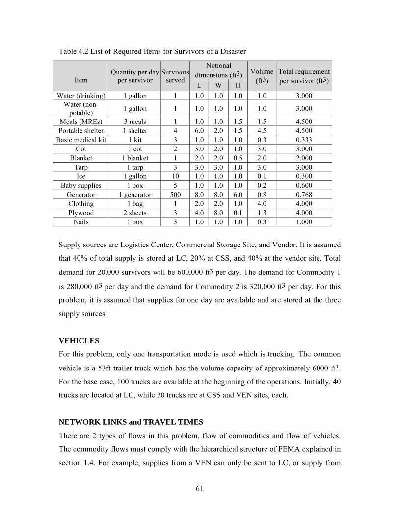
61

Table 4.2 List of Required Items for Survivors of a Disaster

Supply sources are Logistics Center, Commercial Storage Site, and Vendor. It is assumed

that 40% of total supply is stored at LC, 20% at CSS, and 40% at the vendor site. Total

demand for 20,000 survivors will be 600,000 ft3 per day. The demand for Commodity 1

is 280,000 ft3 per day and the demand for Commodity 2 is 320,000 ft3 per day. For this

problem, it is assumed that supplies for one day are available and are stored at the three

supply sources.

VEHICLES

For this problem, only one transportation mode is used which is trucking. The common

vehicle is a 53ft trailer truck which has the volume capacity of approximately 6000 ft3.

For the base case, 100 trucks are available at the beginning of the operations. Initially, 40

trucks are located at LC, while 30 trucks are at CSS and VEN sites, each.

NETWORK LINKS and TRAVEL TIMES

There are 2 types of flows in this problem, flow of commodities and flow of vehicles.

The commodity flows must comply with the hierarchical structure of FEMA explained in

section 1.4. For example, supplies from a VEN can only be sent to LC, or supply from

Item

Quantity per day per survivor

Survivors served

Notional dimensions (ft3)

Volume (ft3)

Total requirement per survivor (ft3)

L W H

Water (drinking) 1 gallon 1 1.0 1.0 1.0 1.0 3.000 Water (non-

potable) 1 gallon 1 1.0 1.0 1.0 1.0 3.000

Meals (MREs) 3 meals 1 1.0 1.0 1.5 1.5 4.500 Portable shelter 1 shelter 4 6.0 2.0 1.5 4.5 4.500

Basic medical kit 1 kit 3 1.0 1.0 1.0 0.3 0.333 Cot 1 cot 2 3.0 2.0 1.0 3.0 3.000

Blanket 1 blanket 1 2.0 2.0 0.5 2.0 2.000 Tarp 1 tarp 3 3.0 3.0 1.0 3.0 3.000 Ice 1 gallon 10 1.0 1.0 1.0 0.1 0.300

Baby supplies 1 box 5 1.0 1.0 1.0 0.2 0.600 Generator 1 generator 500 8.0 8.0 6.0 0.8 0.768 Clothing 1 bag 1 2.0 2.0 1.0 4.0 4.000 Plywood 2 sheets 3 4.0 8.0 0.1 1.3 4.000

Nails 1 box 3 1.0 1.0 1.0 0.3 1.000

62

LC can be sent to all MOBs and FOSAs. Supplies in MOBs can be sent to other MOBs or

to FOSAs. Supplies from FOSAs can be sent to other FOSAs and to SSAs, as long as it

remains in the same State. Supplies received at each SSA can be sent to other SSAs in the

same State or must be delivered to PODs of that State.

The flow of vehicles in the network is much less restricted compared to commodity

flows. It is assumed that there is a link between each pair of nodes in the network.

Basically, empty vehicles are free to travel between each two nodes of the network

without the need to visit any intermediate nodes. As a result, when a vehicle is carrying

supplies, it must follow the more restricted hierarchical network of FEMA. But when the

vehicle unloads all its supply, either at intermediate nodes or final PODs, it is free to go

to any other node in the network to pick up supplies and start a new round of delivery.

Link travel time functions for the proposed formulation can be completely arbitrary. The

formulation is capable of dealing with time-variable travel times as well as fixed travel

times. For this numerical study, the travel distance between any two nodes of the network

is assumed to be equal to their Euclidian distance. The travel speed is assumed to be fixed

for all the vehicles on the federal level network (between LC, CSS, VEN, MOBs, and

FOSA) and to be equal to 50 miles per hour. However, for State level network (between

FOSAs, SSAs, and PODs) the travel speed is assumed to be 40 miles per hour.

TIME SCALE

Selection of appropriate time step is a very important factor that can affect the

performance of time-space networks dramatically. For each time period in the planning

horizon, one layer of physical network will be added to the problem. This makes the

problem size grow extremely fast with the number of time steps in the planning horizon.

For example if the planning horizon is only 1 day, with the choice of time step t = 5

minutes, it will be 24 * 60 / 5 = 288 layers of the network. So to keep the problem at a

reasonable size, it is favorable to have long time steps.

63

On the other hand, shorter time steps will improve the accuracy of modeling the

emergency response operations. For example if the time step is 1 hour, it is possible to

model the state of the system only at every hour and not at the times in between. So from

the accuracy perspective, it is favorable to have shorter time steps.

The other important issue in determining the time-step in this problem is the issue of

dealing with very long and very short links. At the federal level network, nodes are

usually far from each other and the links can range from a hundred miles to a few

thousand miles. The travel time on those links with ground transportation can range from

a few hours to up to one day or more. However, the nodes at the lower levels in the State

networks can be very close to each other. It is very common to have PODs that are only a

few miles apart. In this case, link travel times can be in the order of minutes. Figure 4.6

better shows the issue of scale in this problem on the disaster area map.

It is a difficult challenge to select a time-step that is suitable for very short links and very

long links, at the same time. A very short time-step is necessary to model the short links

even though it will increase the problem size very quickly. But the main issue is the

sensitivity of travel times to the selected time-step. If a very short time-step is chosen, say

1 minute, it might be good for short links but the travel times on very long links will not

be sensitive to that. It is very difficult, if not impossible, to predict the travel time

between two nodes that are a thousand miles apart, with accuracy of 1 minute. For those

links the 1-hour unit or 30-minute unit is more meaningful.

64

Figure 4.6 Issue of Scale in Disaster Area

GEOGRAPHICAL DECOMPOSITION

To deal with this issue, a geographical decomposition method is proposed. The nodes at

federal level (LC, CSS, VEN, MOB, FOSA) will be in one subset and the nodes at each

State (FOSA, SSA, POD) will form another subset. Since the travel times between nodes

in federal level network are usually long, it is possible to use a large time-step for them.

Using similar argument, the State level nodes and links can be modeled with a short time-

step. Figure 4.7 shows this decomposition.

Now the important issue is how to connect these separate time-space networks. Luckily,

the special structure of FEMA’s supply chain offers the candidates. Federal Operational

Staging Areas (FOSA) are the one and only interface between flow of commodities in

federal level facilities and the designated state level facilities. We take advantage of this

opportunity and select the FOSAs as transfer terminals between the sub-networks.

For this numerical study, time-step for federal zone, 1t , is chosen to be 30 minutes and

time-step for state level zones, 2t , is selected to be 5 minutes. The travel times for this

study are calculated based on the distance and a fixed average travel speed explained

65

earlier. So based on the newly defined time steps of 1t and 2t , travel times of federal zone

links are being rounded to the nearest 30 minute interval and the travel times of state

level zone links are being rounded to the nearest 5 minute.

Figure 4.7 Geographical Decomposition for Time Steps

How the FOSA nodes connect two sub-networks with different time steps is shown in

Figure 4.8. This graph indicates that the arcs entering FOSA from federal network or

leaving the FOSA toward the federal network can exist only at 1t =30-minute intervals.

But the arcs that connect FOSA to state level facilities exist for every 2t =5-minute

interval. The implication is that the downward flows (from federal network to state

network) entering a given FOSA can leave that FOSA at any 5-minute period after that.

However, the upward flows (from state network to federal network) that enter a FOSA at

any time other than 30-minute intervals, need to wait at the FOSA until the first available

30-minute interval.

VEN LC CSS

MOB MOB

FOSA FOSA

SSA SSA SSA SSA

POD POD POD POD POD

POD

fed

St1 St2

66

Figure 4.8 Time-Space network with Different Time Steps at FOSA

4.2. Generating Formulation and Commercial Solver

The sample problem introduced previously is a fairly large mixed integer program with

real valued, general integer, and binary variables. Because of the large number of

variables and constraints in this problem, computer programs are required to handle the

input and output data. A customizable program is coded in the Microsoft Visual Studio

environment to generate the formulation for each problem instance. The program receives

the input data from the prepared data files as well as the coded user interface to generate

each problem instance. Then the mathematical formulation for each problem instance is

generated and written to a text file.

FOSA

State-Level Nodes

Federal-Level Nodes

Time period 0 1 2 3 4 5 6 7 8 9 10 11 12

t2

t1

Downward Flow Upward Flow Carry-over Flow

67

At this stage, the numerical sample problems are solved with CPLEX (2006). CPLEX is a

commercial optimization package from ILOG Company that solves mathematical

formulations in the forms of linear programs (LP), integer programs (IP), and quadratic

programs (QP). CPLEX reads the generated formulations from text files, after

optimization the results are written to text files as well. Another customized program is

coded to extract the results from the output file and generate the required performance

measures and charts.

4.3. Numerical Results and Analysis

To better evaluate the characteristics of the proposed model, 10 numerical case studies

are generated. All the case studies are based on the described imaginary scenario with

variations in the subset of enforced constraints and some parameter values. Table 4.3

describes the considered case studies. In general, the case studies in tables 4.3 start from

simple and become more complicated toward the end. For example, the first case study

only considers the conservation of flow and vehicle capacity constraints. Other

constraints are gradually added to the formulation in the other case studies up to Case 7

which has the largest number of constraint types for a one day operation. First 7 case

studies consider only 1 day of operations while in the last 3 cases 2 days of operations are

formulated.

Table 4.4 summarizes the optimization results for all 10 case studies. Case-1 is the “base

case” with only conservation of flow constraint and vehicle capacity constraints modeled

for 1 day of operations. The solver found the optimal solution in approximately 4

minutes. Figure 4.9 shows the percent of unsatisfied demand for all victims over time.

The first delivery to the nearest demand point took about 7 hours. Fifty percent of the

total demand was satisfied after 11 hrs and 40 minutes. The last demand was served after

21 hours and 40 minutes.

68

Table 4.3 Numerical Case-Study Descriptions

Case Number

Constraints Used Details Variables

ConstraintsFile Size

(Kb) Real Val. Integer

1 Flow Conservation + Vehicle Capacity 1 day

100 Trucks 133,275 157,972 81,891 13,331

2 Flow Conservation + Vehicle Capacity 1 day

200 trucks 133,275 157,972 81,891 13,331

3 Flow Conservation + Vehicle Capacity + Facility Capacity

1 day 100 Trucks

133,275 157,972 87,094 15,846

4 Flow + Facility Location (2,2,5)* + Facility Capacity 1 day

100 Trucks 133,275 157,972 87,094 15,846

5 Flow + Facility Location (2,2,2) + Facility Capacity 1 day

100 Trucks 133,275 157,972 87,094 15,846

6 Flow + Facility Capacity Const.+ Equity-1 Const 1 day

100 Trucks 133,275 157,972 87,174 17,214

7 Flow + Facility Location (2,2,5) + Facility Capacity + Equity-1,2,3 Const

1 day 100 Trucks

133,275 157,972 87,294 61,084

8 Flow Conservation + Vehicle Capacity, day by day Supply

2 days 100 Trucks

265,995 315,316 163443 27,439

9 Flow + Facility Location (2,2,5) + Facility Capacity , day by day Supply

2 days 100 Trucks

265,995 315,316 173,878 32,673

10 Flow + Capacity + location (2,2,5) , 2 day supply available

2 days 100 Trucks

265,995 315,316 173,878 32,673

* Facility location with maximum number of (MOB, FOSA, SSA)

69

Table 4.4 Summary of Optimization Results

Case Number

Objective Value

Last UD (hr:min)

Temp. Facilities

Root Sol. Time (s)

Iterations CPU Time

(sec)†

1 9.0798 E+07 21:40 (4,4,10) 33.89 14,957 230

2 8.6118 E+07 15:10 (4,4,10) 10.36 5,502 20

3 1.0412 E+08 22:05 (4,4,10) 42.73 18,642 778

4 1.0412 E+08 22:05 (2,2,5) 33.59 17,308 945

5 1.0978 E+08 24:00§ (2,2,2) 204.19 205,588 5575

6 1.0439 E+08 21:50 (4,4,10) 42.22 5,810,980 45856*

7 1.0417 E+08 22:05 (2,2,5) 63.09 7,888,315 81642*

8 1.7985 E+08 39:10 (4,4,10) 786.34 63,960 4779

9 2.0859 E+08 44:45 (2,2,5) 2450.91 408,351 14635

10 1.8921 E+08 48:00§ (2,2,5) 10117.11 2,963,071 231035

* The solver stopped prematurely with “out of memory” error message. § The relief operations were not finished by the assumed horizon. † On a 3.0 GHz Intel Pentium CPU with 2.0 GB RAM Case-2 is similar to Case-1 but the only difference is that there are 200 trucks available in

Case-2 versus 100 trucks in Case-1. Even tough the number of vehicles was increased,

the optimal solution was found in only 20 seconds. As it can be seen in Table 4.3, the size

of the formulation (number of variables and constraints) for Case-2 is equal to Case-1 and

this is one of the important advantages of current formulation. Since this formulation

treats the vehicles as commodities, the number of available vehicles appears only as a

right-hand-side parameter and does not have an effect on the problem size. Figure 4.10

shows the percent of unsatisfied demand over time for Case-2 at optimality. Since there

were enough vehicles at the beginning, the vehicles did not need to return to the sources

70

to pick up supplies once they had left. As a result, the delivery operations were completed

after only 15 hours and 10 minutes.

Figure 4.9 Percent of unsatisfied demand over time for CASE 1

Figure 4.10 Percent of unsatisfied demand over time for CASE 2

0

10

20

30

40

50

60

70

80

90

100

0 2 4 6 8 10 12 14 16 18 20 22 24Time (hr)

Un

sa

tis

fie

d D

em

an

d (

%)

0

10

20

30

40

50

60

70

80

90

100

0 2 4 6 8 10 12 14 16 18 20 22 24Time (hr)

Un

sa

tis

fie

d D

em

an

d (

%)

71

Case 3 is similar to the base-case with addition of loading, unloading, and storage

capacities for all facilities. In this case, there is no limitation on the maximum number of

temporary facilities and all the potential sites can be active. Figure 4.11 shows the

variation of unsatisfied demand for Case-3. The addition of facility capacities prevented

the shipment and delivery of large quantities of supplies. Instead, the relief commodities

are delivered more uniformly over time compared to Case-1 and Figure 4.9.

Consequently, the objective function value was higher and the operation took 22 hr and 5

minutes, 25 minutes more than Case-1. The running time was also increased to about 13

minutes to find the optimal solution.

In Case 4 we limited the maximum number of temporary facilities (MOB, FOSA, SSA)

to (2, 2, 5) plus the constraints of Case-3. It took the solver about 16 minutes to find the

optimal solution which is 3 minutes more than Case-3. However, the objective function

value at optimality is the same for Case-3 and Case-4. Also the time of last delivery was

the same. This implied that even though we limited the number of temporary facilities to

(2, 2, 5); it was still possible to run the operation and achieve the same results.

Comparing Figure 4.12 with 4.11 shows that there were minor changes in the flow of

commodities, but the results are very similar.

Figure 4.11 Percent of unsatisfied demand over time for CASE 3

0

10

20

30

40

50

60

70

80

90

100

0 2 4 6 8 10 12 14 16 18 20 22 24Time (hr)

Un

sa

tis

fie

d D

em

an

d (

%)

72

Figure 4.12 Percent of unsatisfied demand over time for CASE 4

In order to see the effect of limited number of facilities, we created Case-5 with

maximum number of temporary facilities as (2, 2, 2). Table 4.4 shows that problem

became much harder. The running time jumped to 1.5 hours. The objective function was

increased and more importantly, the delivery operations could not be finished in 24

hours. Figure 4.13 shows that at the end of 24 hours, there is still unsatisfied demand

which is about 6% of total demand. This indicated that unlike Case-4, limiting the

number of temporary facilities had affected the operations resulting in more delays and

more sufferings.

In Case-6 we added the equity constraints to the problem for the first time. At this stage,

only the 1st equity constrains (Equation 3.24) were considered in addition to conservation

of flow and vehicle capacity constraints. Table 4.4 shows very interesting results. First of

all, adding the equity-1 constraint made the problem much harder. After 13 hours of

execution time and more than 5.8 million iterations, the solver still could not find the

0

10

20

30

40

50

60

70

80

90

100

0 2 4 6 8 10 12 14 16 18 20 22 24Time (hr)

Un

sa

tis

fie

d D

em

an

d (

%)

73

optimal solution. However, the best integer solution found is very close to the best MIP

bound (25500 unsatisfied demands, 0.02% gap).

Finally in Case-7, all the constraints are considered. The constraints include conservation

of flow for the commodities and vehicles, the linkage between commodities and vehicles

and capacity of each vehicle, facility location with maximums of (2, 2, 5); loading,

unloading and storage capacities for all facilities, and finally the 3 equity constraints

(Equation 3.24, 3.25, 3.26). The full problem is very large and difficult problem. After

around 23 hours of CPU time and more than 7.8 million iterations, CPLEX solver

stopped and it could not find the optimal solution. By the way, the best integer solution

found is very close to the best MIP bound (30400 unsatisfied demands, 0.03% gap).

Figure 4.14 shows the unsatisfied demand for the best integer solution found by the

solver.

Figure 4.13 Percent of unsatisfied demand over time for CASE 5

0

10

20

30

40

50

60

70

80

90

100

0 2 4 6 8 10 12 14 16 18 20 22 24Time (hr)

Un

sa

tis

fie

d D

em

an

d (

%)

74

Figure 4.14 Percent of unsatisfied demand over time for CASE 7

Another idea was to extend the relief operations duration from 1 day to 2 days and

analyze its effect on the problem size and behavior. Case-8 through Case-10 was created

to address that idea. Again Case-8 is the base case with conservation of flow and vehicle

capacity constraints. Similar to other cases, it was assumed that 100 trucks are available.

The demands for the second day appear at the beginning of the second day and locations

and quantities are similar to the demands of the first day. In Case-8 it is assumed that

supply for the second day arrives at the beginning of the second day operations to the

same sources as of the day one. Table 4.4 shows that the solution time was around 80

minutes. Comparing 80 minutes for Case-8 with 4 minutes of CPU time for Case-1 shows

the growth rate of problem size and difficulty with time horizon. In this case, the duration

of operation is only doubled however the solution time is rapidly increased by a factor of

20.

Figure 4.15 shows the variations in unsatisfied demand over time. The 1st day’s

operations were finished in approximately 18 hours. As a result of the optimal

distribution of empty trucks for the second day, the relief operations in the second day

were over in only 15 hours and 10 minutes. There were no additional supplies available

0

10

20

30

40

50

60

70

80

90

100

0 2 4 6 8 10 12 14 16 18 20 22 24Time (hr)

Un

sa

tis

fie

d D

em

an

d (

%)

75

before the second day, but modeling the operations for 2-day provided the opportunity to

be prepared and do a better job in the second day.

In Case-9, the facility location constraints with maximum of (2, 2, 5) and the loading,

unloading, and storage capacity constraints were considered for 2 days of operations.

Similar to previous case, the supplies become available day by day. Table 4.4 shows that

adding the capacity constraints has increased the objective function value for about 16%

compared to Case-8. The running time is also increased to more than 4 hours of CPU

time.

Figure 4.16 shows the results of optimal solution for Case-9. Because of the capacity

constraints the flow of large amounts of commodities were prohibited. As a result, the

demands are satisfied gradually over time and for both days, the operations took longer

compared to Case-8. It took 44 hours and 45 minutes to deliver all the supplies in Case-9

compared to 39 hours and 10 minutes in Case-8.

The last case study in this numerical experiment is Case-10. Case-10 is similar to Case-9

with the only variation that all the supplies for 2-days are assumed to be available at the

beginning of the operations. The demands still appear at the start of each day and supplies

can not be delivered beforehand. The objective function of optimal solution shows

approximately 10% reduction compared to Case-9. The reason is that since the supplies

were available at the beginning, they were sent to intermediate nodes close to demand

points so the delivery of supplies for the 2nd day can start as soon as the demands appear

for that day. Figure 4.17 shows the details.

The possibilities in arranging the details of operations in Case-10 are larger than any

other case. Consequently, the CPLEX solver went over 2.9 million iterations and it took

more than 2 days and 16 hours of CPU time to find the optimal solution. It is clear that a

problem with complete set of constraints (if the equity constraints were to be added to the

problem) with 2-days of operations, can not be solved by the commercial solver.

76

Figure 4.15 Percent of unsatisfied demand over time for CASE 8

Figure 4.16 Percent of unsatisfied demand over time for CASE 9

0

10

20

30

40

50

60

70

80

90

100

0 2 4 6 8 10 12 14 16 18 20 22 24 26 28 30 32 34 36 38 40 42 44 46 48

Time (hr)

Un

sati

sfie

d D

eman

d (

%)

0

10

20

30

40

50

60

70

80

90

100

0 2 4 6 8 10 12 14 16 18 20 22 24 26 28 30 32 34 36 38 40 42 44 46 48Time (hr)

Un

sati

sfie

d D

eman

d (

%)

77

Figure 4.17 Percent of unsatisfied demand over time for CASE 10

4.4. Summary

The numerical analysis in this chapter was designed to test the proposed formulation and

evaluate the properties of the optimization problem. 10 different case studies were

generated based on the same structure of the problem to analyze the effect of different

parameters. In general, the proposed modeling framework produced reasonable

outcomes. It was able to provide the level of detail required in the disaster response

logistics at the operational level. For simple cases and small size problems, the

commercial solver was able to find the optimal solutions, however, when the difficult

constraints such as Equity Constraints were added or when the time horizon was

extended from 1-day to 2-days, CPLEX was unable to deliver good results. It is

concluded that better solution algorithms or heuristics are needed to address the larger

problem instances or real world size problems.

0

10

20

30

40

50

60

70

80

90

100

0 2 4 6 8 10 12 14 16 18 20 22 24 26 28 30 32 34 36 38 40 42 44 46 48

Time (hr)

Un

sati

sfie

d D

eman

d (

%)

78

Chapter 5: Conclusions and Future Directions

The global increase in the number of natural disasters highlights the need for a better

planning and operation of the responding agencies. During emergencies various aid

organizations often face significant problems of transporting large amounts of many

different relief commodities including food, clothing, medicine, medical supplies,

machinery, and personnel from different points of origin to different destinations in the

disaster areas. The transportation of supplies and relief personnel must be done quickly

and efficiently to maximize the survival rate of the affected population and minimize the

cost of such operations. It is very difficult, if not impossible, to efficiently operate such a

complex system without comprehensive mathematical models.

Offering a centralized comprehensive model that describes the specifics of disaster

supply chains was the main goal of this research. We aimed at developing a system of

computer and mathematical models to keep track of operational details of large scale

disaster response operations and find the optimal allocation of scarce resources to the

most critical tasks in order to minimize loss of life and human sufferings.

Most of the research in the field of disaster management is related to social sciences and

humanities (Hughes1991).The existing academic literature is relatively light on disaster

management articles that used operations research or management science (OR/MS)

techniques to deal with the problem. This study provided a compendium of previous

research in disaster management with focus on OR/MS techniques and analyzed the

advantages and disadvantages of the works available in the literature.

Initial investigations in this research showed that FEMA has a complex supply chain

spreading across the country to coordinate with its state and local government

counterparts and with nonprofit and for-profit organizations. To the best of our

knowledge, there was no study in the academic literature that provided a systematic view

of the FEMA’s supply chain. This research was able to investigate and summarize

FEMA’s structure into seven main components and showed the relations between them as

a network. The proposed network representation was the key factor that made the

mathematical modeling of the FEMA’s special logistics structure possible.

79

The results of this research extended the state-of-the-art by presenting an integrated

model at the operational level that describes the details of supply chain logistics in major

emergency management agencies such as FEMA, in response to immediate aftermath of

a large scale disaster. The proposed model controls the flow of all the relief commodities

from the sources through the chain and until they are delivered to the hands of recipients.

The proposed model not only considers details such as vehicle routing and pick up or

delivery schedules; but also considers finding the optimal location for temporary facilities

as well as considering the capacity constraints for each facility and the transportation

system. This model provided the opportunity for a centralized operation plan that can

eliminate delays and assign the limited resources in a way that is optimal for the entire

system.

Applying the proposed model on a series of case-study scenarios verified the model and

showed its capabilities to handle large-scale problems. Using the proposed model

provided high level of transparency and control over the disaster response operations that

was not available before.

The following directions are suggested for future researches in this area:

1- Introduce a set of solution techniques and heuristic algorithms to solve the MIP

problem for large cases in short times. It was shown in the analysis of numerical

results that for the large scale problems, commercial solvers were not able to find

the optimal solution for proposed model or the running time was so long that it was

not practical for disaster response management at the operational level. Two main

approaches can be followed to develop heuristic solution techniques. In the first

approach, the model can be decomposed into a number of smaller/easier problems

and then try to aggregate the results. The decomposition can be spatial or temporal

or both. In the second approach, the idea can be to develop heuristics that find near

optimal solutions for the entire model in a short time. Various relaxation

techniques may be used for this type of heuristics. At the end, the results of the two

approaches can be compared to each other.

80

2- Find a tight lower bound for the MIP problem, in order to evaluate the quality of

solutions provided by the heuristic algorithms. It is very important to have a

relatively close bound because for the large size problems, a theoretical bound is

the only benchmark to compare the quality of different heuristics. If a tight bound

is provided, that opens up the opportunity to try more ambitious heuristics that can

potentially be very rewarding.

3- Construct real-world-size case studies and a set of simulation experiments to

analyze the model behavior in the large scale disaster response operations. The

disaster relief operations can happen in large and disperse geographical areas

which requires management tools capable of handling the large scale operations.

The dynamic environment after the disaster strike will be best replicated through a

set of well-designed simulation experiments that covers a wide range of possible

scenarios and test the model’s ability to react to variations of data over time.

4- Perform major sensitivity analysis on the model structure and solution algorithms.

The proposed model includes several parameters and variables that can affect the

quality of solution as well as the solution time. A major sensitivity analysis on all

of the related parameters is essential in order to thoroughly investigate the

properties of the model and solution algorithms.

81

Bibliography

1. Alexander, D.E. 1993, Natural Disasters. London: UCL Press

2. Altay, N., and Walter G. G. 2006. OR/MS research in disaster operations

management. European Journal of Operational Research, 175, p475-493.

3. Ardekani S. A. and Hobeika A. (1988) Logistics problems in the aftermath of the

1985 Mexico City earthquake. Transportation Quarterly. 42(1), 107-124.

4. Barbarosoglu, G. and Arda,Y., A two-stage stochastic programming framework for

transportation planning in disaster response. Journal of the Operational Research

Society, 2004, 55, 43–53.

5. Barbarosoglu, G., Ozdamar, L. and Cevik, A., An interactive approach for

hierarchical analysis of helicopter logistics in disaster relief operations. European

Journal of Operational Research, 2002, 140, 118–133.

6. Beamon, B., 1998. "Supply Chain Design and Analysis: Models and Methods",

International Journal of Production Economics, Vol. 55, No. 3, pp. 281-294.

7. Beamon, B., Measuring supply chain performance. International Journal of

Operations & Production Management; 1999, Vol. 19 Issue 3/4, p275-292.

8. Beamon, B. and Kotleba, S., Inventory Modeling for complex emergencies in

humanitarian relief operations. International Journal of Logistics. Vol. 9, No. 1,

March 2006, 1-18.

9. Beamon, B., Humanitarian relief chains: Issues and challenges, in Proceedings of the

34th International Conference on Computers and Industrial Engineering, San

Francisco, CA, 2004.

10. Bodin, L.D., Golden, B.L., Assad, A.A., and Ball, M.O. (1983), "Routing and

scheduling of vehicles and crews. The state of the art", Computers and Operations

Research 10, 69-211.

11. Brown G. G. and Vassiliou A. L. (1993) Optimizing disaster relief: real-time

operational and tactical decision support. Naval Research Logistics (NRL). 40, l-23.

12. Christofides, N., Mingozzi, A., and Toth, P. (1981), "Exact algorithms for the vehicle

routing problem, based on spanning tree and shortest path relaxations", Mathematical

Programming 20, 255-282.

82

13. Crainic TG, Rousseau J-M. Multicommodity, multimode freight transportation: a

general modeling and algorithmic framework for the service network design problem.

Transportation Research B: Methodological 1986; 20:225-242.

14. CRED, Annual Disaster Statistical Review: Numbers and Trends 2007. Center for

Research on the Epidemiology of Disasters. http://www.cred.be/

15. Daskin, M.S., 1995. Network and Discrete Location: Models, Algorithms, and

Applications. Wiley & Sons, New York.

16. Desrochers M, Lenstra J K, Savelsbergh M W P (1990) A classification scheme for

vehicle routing and scheduling problems. European Journal of Operational Research

46: 322–332

17. Dimitruk, Paul. Three keys to supply chain management in times of disaster.

Healthcare Purchasing News. Dec 2005.

18. Drezner, Z., Hamacher, H., 2002. Facility Location: Applications and Theory.

Springer-Verlag, Berlin.

19. Eksioglu, B., Network algorithms for supply chain optimization. Ph.D. Dissertation,

University of Florida 2002.

20. EM-DAT, Emergency Disasters Data Base. http://www.em-dat.net/

21. FEMA Strategic Plan 2008-2013. http://www.fema.gov/about/strategicplanfy08.shtm

22. Fisher, M.L. “Optimal solution of vehicle routing problems using minimum K-trees”,

Operations Research, vol. 42, pp. 626–642, 1994.

23. Golden, B.L., and Assad, A.A. (1988), Vehicle Routing: Methods and Studies, North-

Holland, Amsterdam.

24. Guelat J., Florian M. and Crainic T. (1990) A multimode multiproduct network

assignment model for strategic planning of freight flows. Transportation Science. 24,

25-39.

25. Haddow. G., Jane A. Bullock. J, Coppola. D., Introduction to Emergency

Management, Published by Butterworth-Heinemann, 2007

26. Haghani, A. and Oh, S.C., Formulation and solution of a multi-commodity, multi-

modal network flow model for disaster relief operations. Transport. Res. Part A-

Policy and Practice, 1996, 30(3), 231–250.

83

27. Harland, C.M., 1996. Supply chain management: relationships, chains and networks.

British Academy of Management 7 (Special Issue), S63-S80.

28. Hughes, M.A., 1991. A selected annotated bibliography of social science research on

planning for and responding to hazardous material disasters. Journal of Hazardous

Materials 27, 91–109.

29. Kemball-Cook, D., Stephenson, R. (1984), "Lessons in logistics from Somalia",

Disasters, Vol. 8 pp.57-66.

30. Knott R. (1987) The logistics of bulk relief supplies. Disasters 11, 113-115.

31. Knott R. (1988) Vehicle scheduling for emergency relief management: a knowledge-

based approach. Disasters 12, 285-293.

32. Laporte, G., and Nobert, Y. (1987), "Exact algorithms for the vehicle routing

problem", in: S. Martello, G. Laporte, M. Minoux and C. Ribeiro (eds.), Surveys in

Combinatorial Optimization, North-Holland, Amsterdam, 147-184.

33. Laporte, G., “The vehicle routing problem: an overview of exact and approximate

algorithms”, European Journal of Operational Research, vol. 59, pp. 345–358, 1992.

34. G. Laporte, “Vehicle routing”. In Dell’Amico, Maffioli & Martello (Eds.) Annotated

Bibliographies in Combinatorial Optimization. New York, Wiley, 1997.

35. Magnanti,TL,. 1981. Combinatorial Optimization and Vehicle Fleet Planning:

Perspectives and Prospects. Networks 11, 179-2 14.

36. Mentzer, J.T., W. DeWitt, J.S. Keebler, S. Min, N.W. Nix, C.D. Smith, Z.G.

Zacharia. "Defining Supply Chain Management," Journal of Business Logistics,

(22:2), 2001, pp. 1–25.

37. New, S.J., 1997. The scope of supply chain management research. Supply Chain

Management 2 (1), 15-22.

38. New, S.J., Payne, P., 1995. Research frameworks in logistics: three models, seven

dinners and a survey. International Journal of Physical Distribution and Logistics

Management 25 (10), 60-77.

39. Oh, S.C. and Haghani, A., Testing and evaluation of a multi-commodity multi-modal

network flow model for disaster relief management. J. Adv. Transport., 1997, 31(3),

249–282.

84

40. Oloruntoba, R. and Gray, R., Humanitarian aid: an agile supply chain, Supply Chain

Management, 2006, 11(2), 115–120.

41. Owen, S. H. and M. S. Daskin, 1998, “Strategic Facility Location: A Review,”

European Journal of Operational Research, 111, 423-447

42. Ozdamar, L., Ekinci, E. and Kucukyazici, B., Emergency logistics planning in natural

disasters. Ann. Operations Res., 2004, 129, 217–245.

43. Pan American Health Organization. Natural disasters—protecting the public’s health.

Washington DC. (2001)

44. Ray J. (1987) A multi-period linear programming model for optimally scheduling the

distribution of food-aid in West Africa. MSThesis, University of Tennessee,

Knoxville, TN.

45. ReVelle, C. S., Eiselt, H.A., and Daskin, M. S., 2008, “A Bibliography for Some

Fundamental Problem Categories in Discrete Location Science,” European Journal of

Operational Research, 184:3, 817-848.

46. Schilling, D.A., Jayaraman, V. and Barkhi, R., 1993, A review of covering problems

in facility location, Location Science 1 (1) (1993) pp. 25-55.

47. Scott, C., Westbrook, R., 1991. New strategic tools for supply chain management.

International Journal of Physical Distribution and Logistics 21 (1), 23-33.

48. Tan, K.C., 2001. A framework of supply chain management literature. European

Journal of Purchasing & Supply Management 7, 39–48.

49. Thomas, A.S., Humanitarian logistics: enabling disaster response, Fritz Institute,

2007.

50. Thomas, A.S. and Kopczak. L.R., From logistics to supply chain management: The

path forward in the humanitarian sector. Fritz Institute, 2005.

51. P. Toth, D. Vigo (Eds.) (2002).The Vehicle Routing Problem, SIAM Monographs on

Discrete Mathematics and Applications, Philadelphia.

52. Van Wassenhove, L.N., Humanitarian aid logistics: supply chain management in high

gear. J. Oper. Res. Soc., 2006,57(5), 475–489.

53. Yi. W. and Ozdamar, L., A dynamic logistics coordination model for evacuation and

support in disaster response activities. European Journal of Operations Research 179

(2007) 1177-1193.