supplementary note for linear programming

Supplementary note for linear programming

1 Farkas’ Lemma and Theorems of the Alterna-

tive

Lemma 1.1 (Farkas’ Lemma). Let A ∈ Rm×n and c ∈ Rn be a row vector. Suppose

x ∈ Rn is a column vector and w ∈ Rm is a row vector. Then exactly one of the

following systems of inequalities has a solution:

(1) Ax ≥ 0 and cx < 0 or

(2) wA = c and w ≥ 0

Remark 1.2. Before proceeding to the proof, it is helpful to restate the lemma in

the following way:

(1) If there is a vector x ∈ Rn so that Ax ≥ 0 and cx < 0, then there is no vector

w ∈ Rm so that wA = c and w ≥ 0.

1

(2) Conversely, if there is a vector w ∈ Rm so that wA = c and w ≥ 0, then

there is no vector x ∈ Rn so that Ax ≥ 0 and cx < 0.

Proof. We can prove Farkas’ Lemma using the fact that a bounded linear program-

ming problem has an extreme point solution. Suppose that System 1 has a solution

x. If System 2 also has a solution w, then

wA = c =⇒ wAx = cx. (1)

The fact that System 1 has a solution ensures that cx < 0 and therefore wAx < 0.

However, it also ensures that Ax ≥ 0. The fact that System 2 has a solution implies

that w ≥ 0. Therefore we must conclude that:

w ≥ 0 and Ax ≥ 0 =⇒ wAx ≥ 0. (2)

This contradiction implies that if System 1 has a solution, then System 2 cannot

have a solution.

Now, suppose that System 1 has no solution. We will construct a solution for

System 2. If System 1 has no solution, then there is no vector x so that cx < 0 and

Ax ≥ 0. Consider the linear programming problem:

PF

⎧⎪⎪⎪⎨

⎪⎪⎪⎩

min cx

s.t. Ax ≥ 0

(3)

Clearly x = 0 is a feasible solution to this linear programming problem and further-

more is optimal. To see this, note that the fact that there is no x so that cx < 0 and

2

Ax ≥ 0, it follows that cx ≥ 0; i.e., 0 is a lower bound for the linear programming

problem PF . At x = 0, the objective achieves its lower bound and therefore this

must be an optimal solution. Therefore PF is bounded and feasible.

We can convert PF to standard form through the following steps:

(1) Introduce two new vectors y and z with y, z ≥ 0 and write x = y − z (since

x is unrestricted).

(2) Append a vector of surplus variables s to the constraints.

This yields the new problem:

P ′F

⎧⎪⎪⎪⎪⎪⎪⎪⎨

⎪⎪⎪⎪⎪⎪⎪⎩

min cy − cz

s.t. Ay −Az− Ims = 0

y, z, s ≥ 0

(4)

Problem P ′F in which the reduced costs for the variables are all negative (that is,

zj − cj ≤ 0 for j = 1, . . . , 2n+m). Here we have n variables in vector y, n variables

in vector z and m variables in vector s. Let B ∈ Rm×m be the basis matrix at

this optimal feasible solution with basic cost vector cB. Let w = cBB−1 (as it was

defined for the revised simplex algorithm).

Consider the columns of the simplex tableau corresponding to a variable xk (in

our original x vector). The variable xk = yk − zk. Thus, these two columns are

additive inverses. That is, the column for yk will be B−1Ak, while the column for zk

3

will be B−1(−Ak) = −B−1Ak. Furthermore, the objective function coefficient will

be precisely opposite as well.

Thus the fact that zj − cj ≤ 0 for all variables implies that:

wAk − ck ≤ 0 and

−wAk + ck ≤ 0 and

That is, we obtain

wA = c (5)

since this holds for all columns of A.

Consider the surplus variable sk. Surplus variables have zero as their coefficient in

the objective function. Further, their simplex tableau column is simply B−1(−ek) =

−B−1ek. The fact that the reduced cost of this variable is non-positive implies that:

w(−ek)− 0 = −wek ≤ 0 (6)

Since this holds for all surplus variable columns, we see that −w ≤ 0 which implies

w ≥ 0. Thus, the optimal basic feasible solution to Problem P ′F must yield a vector

w that solves System 2.

Lastly, the fact that if System 2 does not have a solution, then System 1 does

follows from contrapositive on the previous fact we just proved.

Problem 1. Suppose we have two statements A and B so that:

4

A ≡ System 1 has a solution.

B ≡ System 2 has a solution.

Our proof showed explicitly that NOT A =⇒ B. Recall that contrapositive is the

logical rule that asserts that:

X =⇒ Y ≡ NOT Y =⇒ NOT X (7)

Use contrapositive to prove explicitly that if System 2 has no solution, then System

1 must have a solution. [Hint: NOT NOT X ≡ X.]

2 Duality

In this section, we show that to each linear programming problem (the primal prob-

lem) we may associate another linear programming problem (the dual linear pro-

gramming problem). These two problems are closely related to each other and an

analysis of the dual problem can provide deep insight into the primal problem.

5

The Dual Problem

Consider the linear programming problem

P

⎧⎪⎪⎪⎪⎪⎪⎪⎨

⎪⎪⎪⎪⎪⎪⎪⎩

max cTx

s.t. Ax ≤ b

x ≥ 0

(8)

Then the dual problem for Problem P is:

D

⎧⎪⎪⎪⎪⎪⎪⎪⎨

⎪⎪⎪⎪⎪⎪⎪⎩

min wb

s.t. wA ≥ c

w ≥ 0

(9)

Remark 2.1. Let v be a vector of surplus variables. Then we can transform Problem

D into standard form as:

DS

⎧⎪⎪⎪⎪⎪⎪⎪⎪⎪⎪⎪⎨

⎪⎪⎪⎪⎪⎪⎪⎪⎪⎪⎪⎩

min wb

s.t. wA− v = c

w ≥ 0

v ≥ 0

(10)

In this formulation, we see that we have assigned a dual variable wi (i = 1, . . . ,m)

to each constraint in the system of equations Ax ≤ b of the primal problem. Like-

wise dual variables v can be thought of as corresponding to the constraints in x ≥ 0.

6

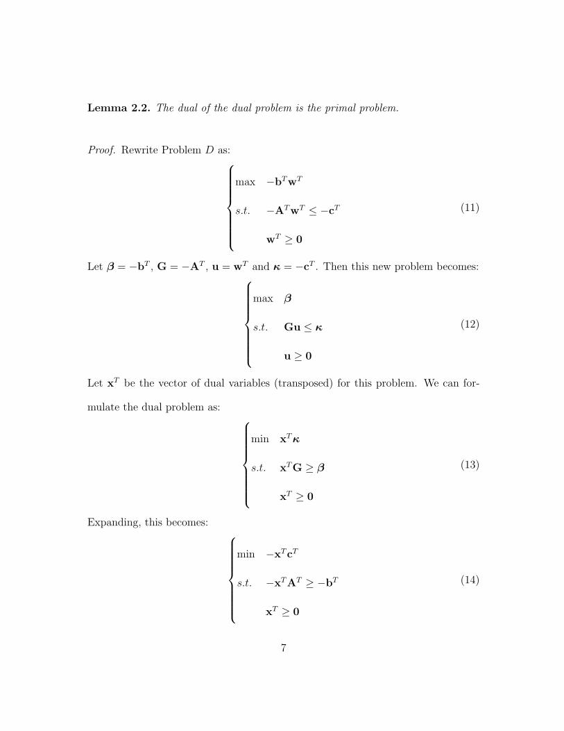
Lemma 2.2. The dual of the dual problem is the primal problem.

Proof. Rewrite Problem D as:⎧⎪⎪⎪⎪⎪⎪⎪⎨

⎪⎪⎪⎪⎪⎪⎪⎩

max −bTwT

s.t. −ATwT ≤ −cT

wT ≥ 0

(11)

Let β = −bT , G = −AT , u = wT and κ = −cT . Then this new problem becomes:⎧⎪⎪⎪⎪⎪⎪⎪⎨

⎪⎪⎪⎪⎪⎪⎪⎩

max β

s.t. Gu ≤ κ

u ≥ 0

(12)

Let xT be the vector of dual variables (transposed) for this problem. We can for-

mulate the dual problem as:⎧⎪⎪⎪⎪⎪⎪⎪⎨

⎪⎪⎪⎪⎪⎪⎪⎩

min xTκ

s.t. xTG ≥ β

xT ≥ 0

(13)

Expanding, this becomes:⎧⎪⎪⎪⎪⎪⎪⎪⎨

⎪⎪⎪⎪⎪⎪⎪⎩

min −xTcT

s.t. −xTAT ≥ −bT

xT ≥ 0

(14)

7

This can be simplified to:

P

⎧⎪⎪⎪⎪⎪⎪⎪⎨

⎪⎪⎪⎪⎪⎪⎪⎩

max cTx

s.t. Ax ≤ b

x ≥ 0

(15)

as required. This completes the proof.

Lemma 2.3. Shows that the notion of dual and primal can be exchanged and that

it is simply a matter of perspective which problem is the dual problem and which is

the primal problem. Likewise, by transforming problems into canonical form, we can

develop dual problems for any linear programming problem.

The process of developing these formulations can be exceptionally tedious, as it

required enumeration of all the possible combinations of various linear and variable

constraints. The following table summarizes the process of converting an arbitrary

primal problem into its dual.

Example 2.4. Consider the following problem:

max 7x1 + 6x2

s.t. 3x1 + x2 + s1 = 120 (w1)

x1 + 2x2 + s2 = 160 (w2)

x1 + s3 = 35 (w3)

x1, x2, s1, s2, s3 ≥ 0

8

MINIMIZATION PROBLEM MAXIMIZATION PROBLEMVARIA

BLES ≥ 0 ≤

CONSTRAIN

TS

≤ 0 ←→ ≥

UNRESTRICTED =

CONSTRAIN

TS

≥ ≥ 0

VARIA

BLES

≤ ←→ ≤ 0

= UNRESTRICTED

Table 1: Table of Dual Conversions: To create a dual problem, assign a dual variable

to each constraint of the form Ax ◦ b, where ◦ represents a binary relation. Then

use the table to determine the appropriate sign of the inequality in the dual problem

as well as the nature of the dual variables.

Here we have placed dual variable named (w1, w2 and w3) next to the constraints to

which they correspond.

The primal problem variables in this case are all positive, so using Table 1 we

known that the constraints of the dual problem will be greater-than-or-equal-to con-

straints. Likewise, we know that the dual variables will be unrestricted in sign since

the primal problem constraints are all equality constraints.

9

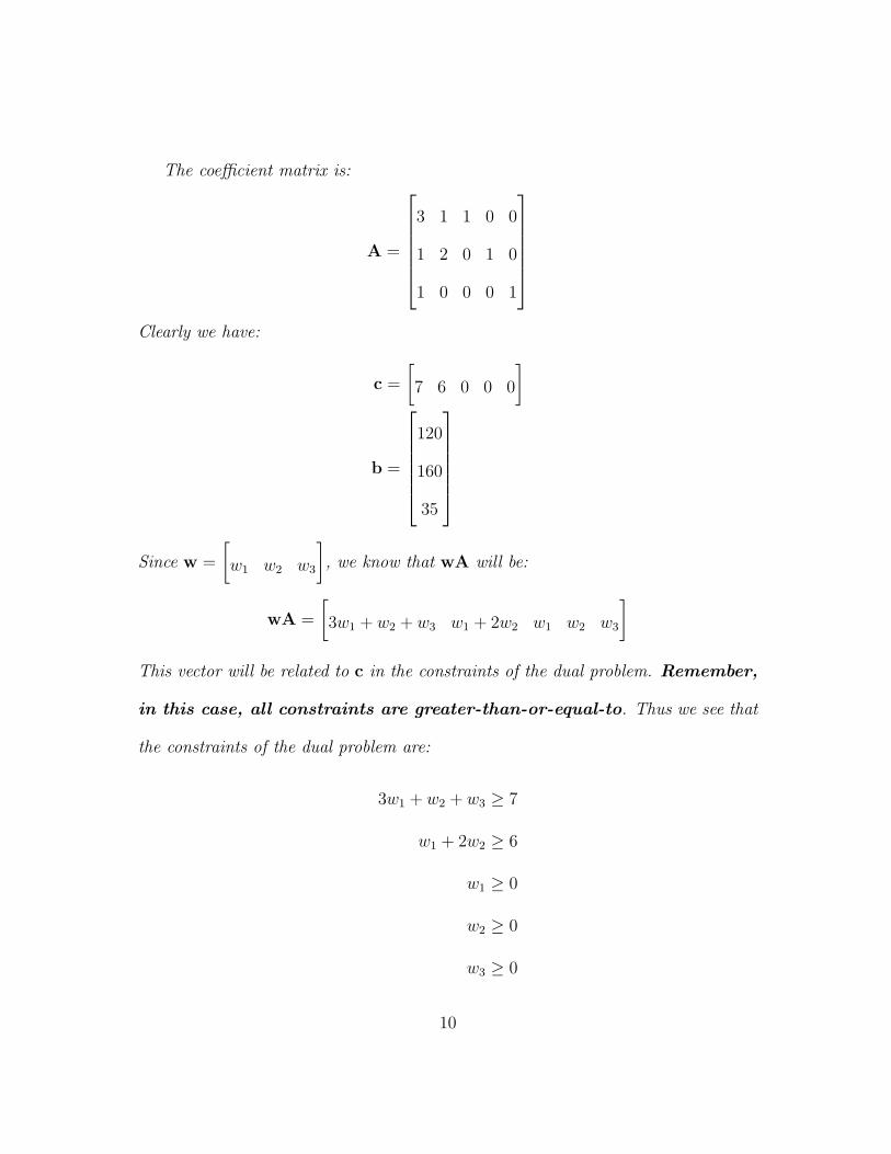
The coefficient matrix is:

A =

⎡

⎢⎢⎢⎢⎢⎣

3 1 1 0 0

1 2 0 1 0

1 0 0 0 1

⎤

⎥⎥⎥⎥⎥⎦

Clearly we have:

c =

[7 6 0 0 0

]

b =

⎡

⎢⎢⎢⎢⎢⎣

120

160

35

⎤

⎥⎥⎥⎥⎥⎦

Since w =

[w1 w2 w3

], we know that wA will be:

wA =

[3w1 + w2 + w3 w1 + 2w2 w1 w2 w3

]

This vector will be related to c in the constraints of the dual problem. Remember,

in this case, all constraints are greater-than-or-equal-to. Thus we see that

the constraints of the dual problem are:

3w1 + w2 + w3 ≥ 7

w1 + 2w2 ≥ 6

w1 ≥ 0

w2 ≥ 0

w3 ≥ 0

10

We also have the redundant set of constraints that tell us w is unrestricted because

the primal problem had equality constraints. This will always happen in cases when

you’ve introduced slack variables into a problem to put it in standard form. This

should be clear from the definition of the dual problem for a maximization problem

in canonical form.

Thus the whole dual problem becomes:

min 120w1 + 160w2 + 35w3

s.t. 3w1 + w2 + w3 ≥ 7

w1 + 2w2 ≥ 6

w1 ≥ 0

w2 ≥ 0

w3 ≥ 0

w unrestricted

(16)

Again, note that in reality, the constraints we derived from the wA ≥ c part of the

dual problem make the constraints “w unrestricted” redundant, for in fact w ≥ 0

just as we would expect it to be if we’d found the dual of the Toy Maker problem

given in canonical form.

11

Problem 2. Identify the dual problem for:

max x1 + x2

s.t. 2x1 + x2 ≥ 4

x1 + 2x2 ≤ 6

x1, x2 ≥ 0

Problem 3. Use the table or the definition of duality to determine the dual for the

problem:⎧⎪⎪⎪⎪⎪⎪⎪⎨

⎪⎪⎪⎪⎪⎪⎪⎩

min cx

s.t. Ax ≤ b

x ≥ 0

(17)

3 Weak Duality

There is a deep relationship between the objective function value feasibility and

boundedness of the problem and the dual problem. We will explore these relation-

ships in the following lemmas.

Lemma 3.1 (Weak Duality). For the primal problem P and dual problem D let x

and w be feasible solutions to Problem P and Problem D respectively, Then:

wb ≥ cx (18)

12

Proof. Primal feasibility ensures that:

Ax ≤ b.

Therefore, we have:

wAx ≤ wb. (19)

Dual feasibility ensure that:

wA ≥ c.

Therefore, we have:

wAx ≥ cx. (20)

Combining Equations 19 and 20 yields Equation 18:

wb ≥ cx.

This completes the proof.

Remark 3.2. Lemma 3.1 ensures that the optimal solution w∗ for Problem D must

provide an upper bound to Problem P , since for any feasible x, we know that:

w∗b ≥ cx. (21)

Likewise, any optimal solution to Problem P provides a lower bound on solution D.

Corollary 3.3. If Problem P is unbounded, then Problem D is infeasible. Likewise,

if Problem D is unbounded, then Problem P is infeasible.

13

Proof. For any x, feasible to Problem P we know that wb ≥ cx for any feasible w.

The fact that Problem P is unbounded implies that for any V ∈ R we can find an

x feasible to Problem P that cx > V . If w were feasible to Problem D, then we

would have wb > V for any arbitrarily chosen V . There can be no finite vector w

with this property and we conclude that Problem D must be infeasible.

The alternative case that when Problem D is unbounded, then Problem P is

infeasible follows by reversing the roles of the problem. This completes the proof.

The Simplex Algorithm

In this section we try to identify some simple way of identifying extreme points. To

accomplish this, let us now assume that we write X as:

X = {x ∈ Rn : Ax = b, x ≥ 0} (22)

We can separate A into an m×m matrix B and an m× (n−m) matrix N and we

have the result:

xB = B−1b−B−1NxN (23)

We know that B is invertible since we assumed that A had full row rank. If we

assume that xN = 0, then the solution

xB = B−1b (24)

14

was called a basic solution. Clearly any basic solution satisfies the constrants Ax =

b but it may not satisfy the constraints x ≥ 0.

Definition 3.4 (Basic Feasible Solution). If xB = B−1b and xN = 0 is a basic

solution to Ax = b and xB ≥ 0, then the solution (xB,xN) is called basic feasible

solution.

Theorem 3.5. Every basic feasible solution is an extreme point of X. Likewise,

every extreme point is characterized by a basic feasible solution of Ax = b, x ≥ 0.

Proof. Since Ax = BxB +NxN = b this represents the intersection of m linearly

independent hyperplanes (since the rank of A is m). The fact that xN = 0 and

xN contains n − m variables, then we have n − m binding, linearly independent

hyperplanes in xN ≥ 0. Thus the point (xB,xN) is the intersection ofm+(n−m) = n

linearly independent hyperplanes. So (xB,xN) must be an extreme point of X.

Converely, let x be an extreme point of X. Clearly x is feasible then it must

represent the intersection of n hyperplanes. The fact that x is feasible implies that

Ax = b. This accounts for m of the intersecting linearly independent hyperplanes.

The remaining n−m hyperplanes must come from x ≥ 0. That is, n−m variables are

zero. Let xN = 0 be the variables for which x ≥ 0 are binding. Denote the remaining

variables xB. We can see that A = [B|N] and that Ax = BxB + NxN = b.

Clearly, xB is the unique solution to BxB = b and thus (xB,xN) is a basic feasible

solution.

15

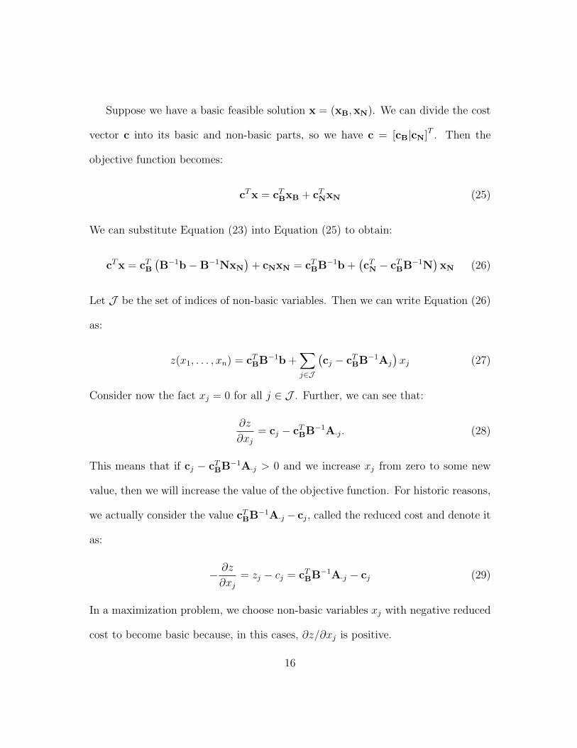
Suppose we have a basic feasible solution x = (xB,xN). We can divide the cost

vector c into its basic and non-basic parts, so we have c = [cB|cN]T . Then the

objective function becomes:

cTx = cTBxB + cTNxN (25)

We can substitute Equation (23) into Equation (25) to obtain:

cTx = cTB(B−1b−B−1NxN

)+ cNxN = cTBB

−1b+(cTN − cTBB

−1N)xN (26)

Let J be the set of indices of non-basic variables. Then we can write Equation (26)

as:

z(x1, . . . , xn) = cTBB−1b+

∑

j∈J

(cj − cTBB

−1Aj

)xj (27)

Consider now the fact xj = 0 for all j ∈ J . Further, we can see that:

∂z

∂xj= cj − cTBB

−1A·j. (28)

This means that if cj − cTBB−1A·j > 0 and we increase xj from zero to some new

value, then we will increase the value of the objective function. For historic reasons,

we actually consider the value cTBB−1A·j − cj, called the reduced cost and denote it

as:

− ∂z

∂xj= zj − cj = cTBB

−1A·j − cj (29)

In a maximization problem, we choose non-basic variables xj with negative reduced

cost to become basic because, in this cases, ∂z/∂xj is positive.

16

Assume we choose xj, a non-basic variable to become non-zero (because zj−cj <

0). We wish to know which of the basic variables will become zero as we increase

xj away from zero. We must also be very careful that none of the variables become

negative as we do this.

By Equation (23) we know that the only current basic variables will be affected

by increasing xj. Let us focus explicitly on Equation (23) where we include only

variable xj (since all other non-basic variables are kept zero). Then we have:

xB = B−1b−B−1A·jxj. (30)

Let b = B−1b be an m × 1 column vector and let that aj = B−1A·j be another

m× 1 column. Then we can write:

xB = b− ajxj. (31)

Let b = [b1, . . . , bm]T and aj = [aj1 , . . . , ajm ], then we have:

⎡

⎢⎢⎢⎢⎢⎢⎢⎢⎣

xB1

xB2

...

xBm

⎤

⎥⎥⎥⎥⎥⎥⎥⎥⎦

=

⎡

⎢⎢⎢⎢⎢⎢⎢⎢⎣

b1

b2

...

bm

⎤

⎥⎥⎥⎥⎥⎥⎥⎥⎦

−

⎡

⎢⎢⎢⎢⎢⎢⎢⎢⎣

aj1

aj2...

bjm

⎤

⎥⎥⎥⎥⎥⎥⎥⎥⎦

xj =

⎡

⎢⎢⎢⎢⎢⎢⎢⎢⎣

b1 − aj1xj

b2 − aj2xj

...

bm − ajmxj

⎤

⎥⎥⎥⎥⎥⎥⎥⎥⎦

(32)

We know (a priori) that bi ≥ 0 for i = 1, . . . ,m. If aji ≤ 0, then as we increase

xj, bi − aji ≥ 0 no matter kow large we make xj. On the other hand, if aji > 0,

then as we increase xj we know that bi − ajixj will get smaller and eventually hit

17

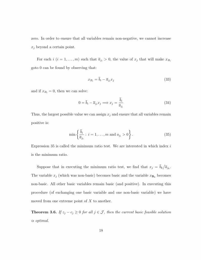
zero. In order to ensure that all variables remain non-negative, we cannot increase

xj beyond a certain point.

For each i (i = 1, . . . ,m) such that aji > 0, the value of xj that will make xBi

goto 0 can be found by observing that:

xBi = bi − ajixj (33)

and if xBi = 0, then we can solve:

0 = bi − ajixj =⇒ xj =biaji

(34)

Thus, the largest possible value we can assign xj and ensure that all variables remain

positive is:

min

{biaji

: i = 1, . . . ,m and aji > 0

}. (35)

Expression 35 is called the minimum ratio test. We are interested in which index i

is the minimum ratio.

Suppose that in executing the minimum ratio test, we find that xj = bk/ajk .

The variable xj (which was non-basic) becomes basic and the variable xBkbecomes

non-basic. All other basic variables remain basic (and positive). In executing this

procedure (of exchanging one basic variable and one non-basic variable) we have

moved from one extreme point of X to another.

Theorem 3.6. If zj − cj ≥ 0 for all j ∈ J , then the current basic feasible solution

is optimal.

18

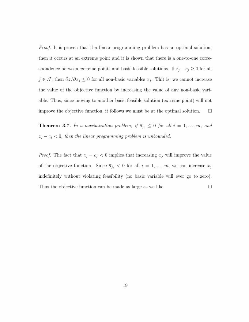
Proof. It is proven that if a linear programming problem has an optimal solution,

then it occurs at an extreme point and it is shown that there is a one-to-one corre-

spondence between extreme points and basic feasible solutions. If zj − cj ≥ 0 for all

j ∈ J , then ∂z/∂xj ≤ 0 for all non-basic variables xj. Thit is, we cannot increase

the value of the objective function by increasing the value of any non-basic vari-

able. Thus, since moving to another basic feasible solution (extreme point) will not

improve the objective function, it follows we must be at the optimal solution.

Theorem 3.7. In a maximization problem, if aji ≤ 0 for all i = 1, . . . ,m, and

zj − cj < 0, then the linear programming problem is unbounded.

Proof. The fact that zj − cj < 0 implies that increasing xj will improve the value

of the objective function. Since aji < 0 for all i = 1, . . . ,m, we can increase xj

indefinitely without violating feasibility (no basic variable will ever go to zero).

Thus the objective function can be made as large as we like.

19

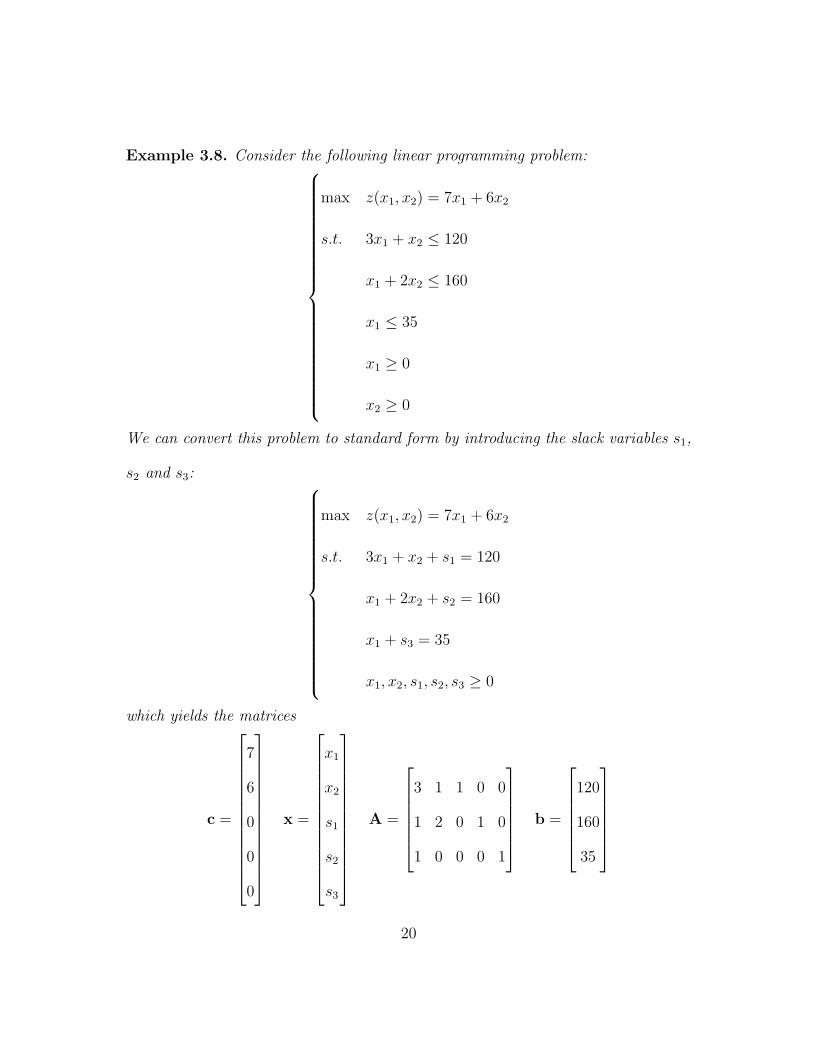
Example 3.8. Consider the following linear programming problem:⎧⎪⎪⎪⎪⎪⎪⎪⎪⎪⎪⎪⎪⎪⎪⎪⎪⎪⎪⎪⎪⎨

⎪⎪⎪⎪⎪⎪⎪⎪⎪⎪⎪⎪⎪⎪⎪⎪⎪⎪⎪⎪⎩

max z(x1, x2) = 7x1 + 6x2

s.t. 3x1 + x2 ≤ 120

x1 + 2x2 ≤ 160

x1 ≤ 35

x1 ≥ 0

x2 ≥ 0

We can convert this problem to standard form by introducing the slack variables s1,

s2 and s3: ⎧⎪⎪⎪⎪⎪⎪⎪⎪⎪⎪⎪⎪⎪⎪⎪⎪⎨

⎪⎪⎪⎪⎪⎪⎪⎪⎪⎪⎪⎪⎪⎪⎪⎪⎩

max z(x1, x2) = 7x1 + 6x2

s.t. 3x1 + x2 + s1 = 120

x1 + 2x2 + s2 = 160

x1 + s3 = 35

x1, x2, s1, s2, s3 ≥ 0

which yields the matrices

c =

⎡

⎢⎢⎢⎢⎢⎢⎢⎢⎢⎢⎢⎢⎣

7

6

0

0

0

⎤

⎥⎥⎥⎥⎥⎥⎥⎥⎥⎥⎥⎥⎦

x =

⎡

⎢⎢⎢⎢⎢⎢⎢⎢⎢⎢⎢⎢⎣

x1

x2

s1

s2

s3

⎤

⎥⎥⎥⎥⎥⎥⎥⎥⎥⎥⎥⎥⎦

A =

⎡

⎢⎢⎢⎢⎢⎣

3 1 1 0 0

1 2 0 1 0

1 0 0 0 1

⎤

⎥⎥⎥⎥⎥⎦b =

⎡

⎢⎢⎢⎢⎢⎣

120

160

35

⎤

⎥⎥⎥⎥⎥⎦

20

We can begin with the matrices:

B =

⎡

⎢⎢⎢⎢⎢⎣

1 0 0

0 1 0

0 0 1

⎤

⎥⎥⎥⎥⎥⎦N =

⎡

⎢⎢⎢⎢⎢⎣

3 1

1 2

1 0

⎤

⎥⎥⎥⎥⎥⎦

In this case we have:

xB =

⎡

⎢⎢⎢⎢⎢⎣

s1

s2

s3

⎤

⎥⎥⎥⎥⎥⎦xN =

⎡

⎢⎣x1

x2

⎤

⎥⎦ cB =

⎡

⎢⎢⎢⎢⎢⎣

0

0

0

⎤

⎥⎥⎥⎥⎥⎦cN =

⎡

⎢⎣7

6

⎤

⎥⎦

and

B−1b =

⎡

⎢⎢⎢⎢⎢⎣

120

160

35

⎤

⎥⎥⎥⎥⎥⎦B−1N =

⎡

⎢⎢⎢⎢⎢⎣

3 1

1 2

1 0

⎤

⎥⎥⎥⎥⎥⎦

Therefore:

cTBB−1b = 0 cTBB

−1N = [0 0] cTBB−1N− cN = [−7 − 6]

Using this information, we can compute:

cTBB−1A·1 − c1 = −7

cTBB−1A·2 − c2 = −6

and therefore:

∂z

∂x1= 7 and

∂z

∂x2= 6

Based on this information, we could choose either x1 or x2 to enter the basis the

value of the objective function would increase. If we choose x1 to enter the basis,

21

then we must determine which variable will leave the basis. To do this, we must

investigate the elements of B−1A·1 and the current basic feasible solution B−1b.

Since each element of B−1A·1 is positive, we must perform the minimum ratio test

on each element of B−1A·1. We know that B−1A·1 is just the first column of B−1N

which is:

B−1A·1 =

⎡

⎢⎢⎢⎢⎢⎣

3

1

1

⎤

⎥⎥⎥⎥⎥⎦

Performing the minimum ratio test, we see have:

min

{120

3,160

1,35

1

}

In this case, we see that index 3 (35/1) is the minimum ratio. Therefore, variable x1

will enter the basis and variable s3 will leave the basis. The new basic and non-basic

variables will be:

xB =

⎡

⎢⎢⎢⎢⎢⎣

s1

s2

x1

⎤

⎥⎥⎥⎥⎥⎦xN =

⎡

⎢⎣s3

x2

⎤

⎥⎦ cB =

⎡

⎢⎢⎢⎢⎢⎣

0

0

7

⎤

⎥⎥⎥⎥⎥⎦cN =

⎡

⎢⎣0

6

⎤

⎥⎦

and the matrices become:

B =

⎡

⎢⎢⎢⎢⎢⎣

1 0 3

0 1 1

0 0 1

⎤

⎥⎥⎥⎥⎥⎦N =

⎡

⎢⎢⎢⎢⎢⎣

0 1

0 2

1 0

⎤

⎥⎥⎥⎥⎥⎦

Note we have simply swapped the column corresponding to x1 with the column cor-

responding to s3 in the basis matrix B and the non-basic matrix N. We will do this

22

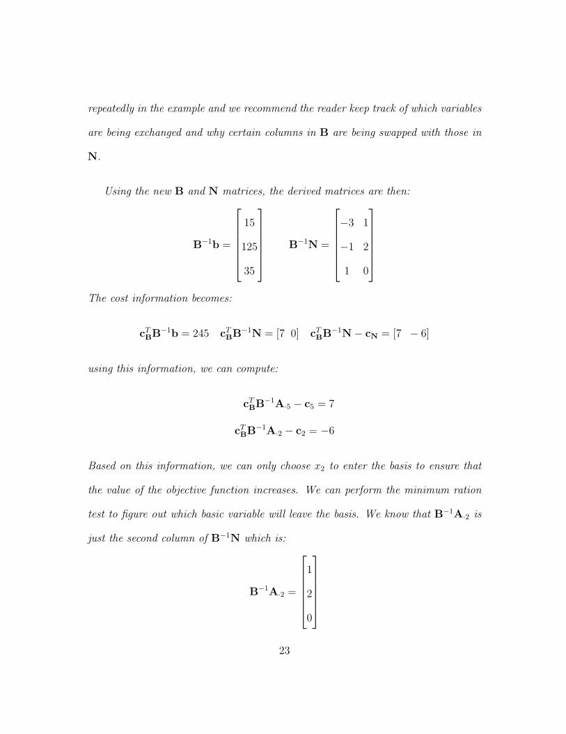
repeatedly in the example and we recommend the reader keep track of which variables

are being exchanged and why certain columns in B are being swapped with those in

N.

Using the new B and N matrices, the derived matrices are then:

B−1b =

⎡

⎢⎢⎢⎢⎢⎣

15

125

35

⎤

⎥⎥⎥⎥⎥⎦B−1N =

⎡

⎢⎢⎢⎢⎢⎣

−3 1

−1 2

1 0

⎤

⎥⎥⎥⎥⎥⎦

The cost information becomes:

cTBB−1b = 245 cTBB

−1N = [7 0] cTBB−1N− cN = [7 − 6]

using this information, we can compute:

cTBB−1A·5 − c5 = 7

cTBB−1A·2 − c2 = −6

Based on this information, we can only choose x2 to enter the basis to ensure that

the value of the objective function increases. We can perform the minimum ration

test to figure out which basic variable will leave the basis. We know that B−1A·2 is

just the second column of B−1N which is:

B−1A·2 =

⎡

⎢⎢⎢⎢⎢⎣

1

2

0

⎤

⎥⎥⎥⎥⎥⎦

23


min

{15

1,125

2

}

In this case, we see that index 1 (15/1) is the minimum ratio. Therefore, variable x2


variables will be:

xB =

⎡

⎢⎢⎢⎢⎢⎣

x2

s2

x1

⎤

⎥⎥⎥⎥⎥⎦xN =

⎡

⎢⎣s3

s1

⎤

⎥⎦ cB =

⎡

⎢⎢⎢⎢⎢⎣

6

0

7

⎤

⎥⎥⎥⎥⎥⎦cN =

⎡

⎢⎣0

0

⎤

⎥⎦


B =

⎡

⎢⎢⎢⎢⎢⎣

1 0 3

2 1 1

0 0 1

⎤

⎥⎥⎥⎥⎥⎦N =

⎡

⎢⎢⎢⎢⎢⎣

0 1

0 0

1 0

⎤

⎥⎥⎥⎥⎥⎦

The derived matrices are then:

B−1b =

⎡

⎢⎢⎢⎢⎢⎣

15

95

35

⎤

⎥⎥⎥⎥⎥⎦B−1N =

⎡

⎢⎢⎢⎢⎢⎣

−3 1

5 −2

1 0

⎤

⎥⎥⎥⎥⎥⎦



−1N = [−11 6] cTBB−1N− cN = [−11 6]

Based on this information, we can only choose s3 to (re-enter) the basis to ensure

that the value of the objective function increases. We can perform the minimum

24

ration test to figure out which basic variable will leave the basis. We know that

B−1A·5 is just the fifth column of B−1N which is:

B−1A·5 =

⎡

⎢⎢⎢⎢⎢⎣

−3

5

1

⎤

⎥⎥⎥⎥⎥⎦


min

{95

5,35

1

}

In this case, we see that index 2 (95/5) is the minimum ratio. Therefore, variable s3


variables will be:

xB =

⎡

⎢⎢⎢⎢⎢⎣

x2

s3

x1

⎤

⎥⎥⎥⎥⎥⎦xN =

⎡

⎢⎣s2

s1

⎤

⎥⎦ cB =

⎡

⎢⎢⎢⎢⎢⎣

6

0

7

⎤

⎥⎥⎥⎥⎥⎦cN =

⎡

⎢⎣0

0

⎤

⎥⎦


B =

⎡

⎢⎢⎢⎢⎢⎣

1 0 3

2 0 1

0 1 1

⎤

⎥⎥⎥⎥⎥⎦N =

⎡

⎢⎢⎢⎢⎢⎣

0 1

1 0

0 0

⎤

⎥⎥⎥⎥⎥⎦

The derived matrices are then:

B−1b =

⎡

⎢⎢⎢⎢⎢⎣

72

19

16

⎤

⎥⎥⎥⎥⎥⎦B−1N =

⎡

⎢⎢⎢⎢⎢⎣

6/10 −1/5

1/5 −2/5

−1/5 2/5

⎤

⎥⎥⎥⎥⎥⎦

25



−1N = [11/5 8/5] cTBB−1N− cN = [11/5 8/5]

Since the reduced costs are now positive, we can conclude that we’ve obtained an

optimal solution because no improvement is possible. The final solution then is:

x∗B =

⎡

⎢⎢⎢⎢⎢⎣

x2

s3

x1

⎤

⎥⎥⎥⎥⎥⎦= B−1b =

⎡

⎢⎢⎢⎢⎢⎣

72

19

16

⎤

⎥⎥⎥⎥⎥⎦

Simply, we have x1 = 16 and x2 = 72.

26

supplementary note for linear programming

Documents