www.sciencemag.org/content/358/6364/776/suppl/DC1

Supplementary Materials for

How the news media activate public expression and influence national

agendas

Gary King,* Benjamin Schneer, Ariel White

*Corresponding author. Email: king@harvard.edu

Published 10 November 2017, Science 358, 776 (2017)

DOI: 10.1126/science.aao1100

This PDF file includes:

Materials and Methods

Figs. S1 to S7

Table S1

References

Contents1 Experimental Design: Additional Information 2

1.1 Units of Analysis . . . . . . . . . . . . . . . . . . . . . . . . . . . . . . 21.2 Randomized Treatment Assignment . . . . . . . . . . . . . . . . . . . . 21.3 Outcome Measurement . . . . . . . . . . . . . . . . . . . . . . . . . . . 41.4 Quantities of Interest . . . . . . . . . . . . . . . . . . . . . . . . . . . . 51.5 Estimation . . . . . . . . . . . . . . . . . . . . . . . . . . . . . . . . . . 71.6 Sequential Hypothesis Tests . . . . . . . . . . . . . . . . . . . . . . . . 91.7 Participating Outlets . . . . . . . . . . . . . . . . . . . . . . . . . . . . 10

2 Additional Results 102.1 Overview . . . . . . . . . . . . . . . . . . . . . . . . . . . . . . . . . . 102.2 Experimental Compliance . . . . . . . . . . . . . . . . . . . . . . . . . 112.3 Hypothesis Tests and Sample Size . . . . . . . . . . . . . . . . . . . . . 112.4 Persuasive Effects on Expressed Opinion . . . . . . . . . . . . . . . . . . 132.5 Additional Observable Implications . . . . . . . . . . . . . . . . . . . . 15

3 Evaluating Sequential Hypothesis Testing 173.1 Theories of Inference . . . . . . . . . . . . . . . . . . . . . . . . . . . . 173.2 Stopping Rules . . . . . . . . . . . . . . . . . . . . . . . . . . . . . . . 183.3 Evaluation Algorithms . . . . . . . . . . . . . . . . . . . . . . . . . . . 19

3.3.1 Parametric Data Generation Process . . . . . . . . . . . . . . . . 203.3.2 Nonparametric Data Generation Process . . . . . . . . . . . . . . 21

3.4 Empirical Results . . . . . . . . . . . . . . . . . . . . . . . . . . . . . . 21

4 Evaluating Heterogeneous Effects 234.1 Leave-One-Outlet-Out Jackknife Estimation . . . . . . . . . . . . . . . . 234.2 Treatment in Week One versus Week Two . . . . . . . . . . . . . . . . . 254.3 Variation in Effects by Experiment . . . . . . . . . . . . . . . . . . . . . 26

5 Social Media Posts as an Outcome Variable 275.1 Composition of Social Media Posts . . . . . . . . . . . . . . . . . . . . . 27

5.1.1 Political Content on Twitter . . . . . . . . . . . . . . . . . . . . 275.1.2 Social Media Post Authorship . . . . . . . . . . . . . . . . . . . 27

5.2 Measuring Twitter User Characteristics . . . . . . . . . . . . . . . . . . 295.3 Logged Outcome Variable . . . . . . . . . . . . . . . . . . . . . . . . . 305.4 Choosing Policy Areas and Keywords . . . . . . . . . . . . . . . . . . . 30

5.4.1 Policy Areas . . . . . . . . . . . . . . . . . . . . . . . . . . . . 305.4.2 Keywords . . . . . . . . . . . . . . . . . . . . . . . . . . . . . . 31

5.5 Coder Training Procedures . . . . . . . . . . . . . . . . . . . . . . . . . 325.6 Automated Text Analysis Procedures . . . . . . . . . . . . . . . . . . . . 32

6 Experimental Interventions 346.1 Comparison between Normal and Treatment Articles . . . . . . . . . . . 346.2 Checking for News Shocks . . . . . . . . . . . . . . . . . . . . . . . . . 356.3 Outlet Audience Size . . . . . . . . . . . . . . . . . . . . . . . . . . . . 37

1

1 Experimental Design: Additional Information

1.1 Units of Analysis

In most social science media experiments, the unit of analysis is an individual research

subject, and the subjects cannot interact with each other. In such a design, individual sub-

jects are randomized to treated and control groups, one hundred research subjects means

n = 100, simple model-free statistical methods can be used (such as the difference in

means), and the scale of the research can remain relatively modest. In contrast, the cost

of the realism we seek is a much larger scale experiment at a more aggregated level, espe-

cially since we aim to continue to avoid spillover effects and the associated assumptions

and more complicated, model dependent statistical techniques. The main issue we have

to contend with is that news media outlets intend to influence the entire national conver-

sation, and thus all potential research subjects (i.e., all Americans who could potentially

be influenced by a story to speak up on social media). Each random assignment of an

article to a news media outlet for publication in a chosen week — which we refer to as an

experiment — can potentially affect millions of people but still constitutes n = 1.

Thus, to avoid spillover effects, our real world intervention uses a unit of treatment that

aggregates all research subjects to the level of an experiment-week — a set of articles to be

written and published on the day (usually Tuesday) of a week we (randomly) determine.

Since we can construct daily measures for our outcome variable, opinions expressed on

social media, we define our unit of analysis as the experiment-day, with up to six days per

week.

1.2 Randomized Treatment Assignment

Our research design, which we constructed to be consistent with the goals of both our

professional journalists and our research team, takes advantage of the fact that, for certain

types of stories, media outlets are indifferent to some aspects of the timing of publication.

We use these points of indifference to introduce randomized treatment interventions with

all the benefits of full experimental control, without logistical or ethical concerns.

To be more specific, we use a version of a matched pair randomized experiment, which

2

has substantially more statistical efficiency, power, and robustness to experimental fail-

ures, and less potential for bias and model dependence, than a completely randomized

experiment (44). If this were a completely randomized experiment, one coin would be

flipped for each unit (each experiment-week) to determine treatment or control status. In-

stead, we match experiment-weeks in pairs prior to treatment assignment, as described

below. We then flip only one coin for the pair, where heads indicates the first week re-

ceives treatment and the second control, and tails is the reverse. This means that variables

that we are able to match exactly are perfectly balanced between the two groups of weeks,

without having to rely on random chance or averaging over larger numbers of observa-

tions. Variables that are only approximately matched still serve to reduce statistical bias,

imbalance between the treated and control groups, and model dependence.

To ensure similarity within each matched pair, we follow two procedures. First, we

approximately match on time by choosing consecutive weeks for each pair. Obviously,

we cannot exactly match on time (since we cannot both intervene and not intervene on

any one day, or divide Americans into disjoint groups that do not communicate). For-

tunately, our preliminary analyses, including trial runs of our experiment, suggest that

the effect of an intervention on one day may last up to about three days but usually less

than a full week. This was confirmed in our present experiment by examining website

pageviews of our treatment articles, which we found declined 95.7% on average from day

1 to day 6. Interventions closer than a week apart thus risk spillover effects (and SUTVA

violations), which would require more complicated statistical methods that may increase

model dependence, and allowing more than a week would unnecessarily risk some im-

balance and lose some efficiency. Restricting interventions to the same day of the week

(usually Tuesday), as we do, also eliminates some volume and viewership imbalances.

Second, we choose a pair of (consecutive) weeks that, so far as we are able to forecast,

will not differ with respect to events in and discussion about our chosen policy area and

subject. We then avoid any remaining bias due to unpredictable news events by randomly

assigning treatment to one of the two weeks within each pair. In other words, we exactly

match on our forecast (or equivalently, we approximately match on actual events), and

3

then randomly balance on surprise events. For example, we would not run an experiment

in the immigration policy area if the president is due to give a speech on immigration

during one of the two weeks. Fortunately, a large number of real world events are highly

predictable, such as government reporting, major conferences, treaty signings, corporate

earnings reports, court cases, planned protests, etc. This exact matching procedure then

reduces the number of observations needed, but it also changes the quantity of interest to

media effects during “quiet” weeks which may be smaller than those at other times.

Finally, to assign treatment, immediately before our chosen two week period, the pack

of 2–5 selected outlets write their newspaper articles (or the equivalent) on the agreed

upon subject within our chosen policy area (approximately one article per outlet). We

then flip a coin and randomly assign one of the two consecutive weeks to the treated

group and the other to the control group. During treated weeks, we instruct the outlets to

do what they normally would do with new content, and publish and promote the newly

written stories, beginning usually on a Tuesday. In control weeks, we ask the outlets to

try to not publish more than usual on the subject of the experiment.

1.3 Outcome Measurement

For variables constructed from social media data, measuring aspects of the national con-

versation, we tap into the so-called full “fire hose” of all tweets from Twitter. (Social

media is usually used to measure a different quantity of interest, but it has been shown to

be predictive of classically measured public opinion (53).) To estimate the number and

opinions of social media posts within each of our broad policy areas, for the total overall

and for those agreeing with our published articles, we use the approach to automated text

analysis described in S5.6. To do this, we defined for each policy area a set of mutually ex-

clusive and exhaustive categories with posts that were (a) in favor of the published articles

in our intervention, (b) opposed to this position, (c) neutral, and (d) off-topic (where the

total is the sum of all posts in categories (a)–(c), and the total agreeing with our published

articles is the number in (a)). See also Section S5.5.

To estimate the number of social media posts on the more specific subject of each

of the published articles, and to define the broad policy areas, we use keyword selection

4

methods and ideas in King, Lam, and Roberts (54). They demonstrated, for selecting

textual documents representing a specific concept, that when individuals act alone they

almost always choose inadequate keyword sets. We thus used the recommended steps of

having multiple people, with human-in-the-loop automated methods, to define better sets

of keywords.

We collect article publication data from media outlet RSS feeds, supplemented by

some manual checks. We obtain data on the number of website pageviews per day for

each of the articles by obtaining access from a sample of the outlets of their Google

Analytics accounts. Pageview data has important competitive value for each outlet and

so is normally a closely guarded secret; we obtained these data only after establishing

high degrees of trust, with the understanding that we would not share the data with other

outlets and only make available the aggregated information we need for this paper.

We have some missing data in the number of articles published (due to errors in how

RSS feeds were set up by certain media outlets) and web pageviews (due to technical

issues in how Google Analytics was installed and, in some cases, whether the outlets

were willing to share their data). We searched extensively for patterns in the missing

data. We did find that we had slightly more data on articles published, and slightly less

Google Analytics data, from the larger media outlets than the smaller ones, but in no

case were we able to detect a pattern that suggested inferential biases. More importantly,

we had no missing data in our outcome variables derived from social media data, or our

treatment variable, which we randomly assigned, and so the possibility of missing data

biasing estimates of our primary quantity of interest is remote.

See Section S5 for additional details.

1.4 Quantities of Interest

Define indices p (p = 1, ..., 11) for the policy area, e (1, . . . , Ep) for the experiment run

within policy area p, and d (d = 1, ..., 6) for the day — 1 for the day of the intervention

(usually Tuesday), 2 for the next day, etc. Then let yped be a count of the number of

social media posts within policy area p, experiment e, and day d. Our treatment, which

parallels the role of the project manager, is the instruction to the chosen pack of 2–5

5

news media outlets participating in an experiment to write and publish articles, within the

broad policy areas we determine, on the agreed upon subject, and on a week we randomly

select from the pair of weeks. Thus, for each policy area p and experiment e, set the

treatment indicator Tped in treated weeks to Tpe1 = ⋅ ⋅ ⋅ = Tpe6 = 1 and in control weeks

to Tpe1 = ⋅ ⋅ ⋅ = Tpe6 = 0.

Our main causal quantity of interest, then, is the total, intent-to-treat effect of our in-

tervention on the extent to which Americans are moved to express their opinions publicly

in a broad policy area we choose. Denote the potential outcomes as yped(1) and yped(0)— the values the outcome variable yped would take under treated and control conditions

respectively, only one of which is observable depending on the actual realized value of

T . Then our quantity of interest for day d is the divergence in potential outcomes aver-

aged over policy areas p and experiments e within those areas, and expressed as either a

difference in numbers of social media posts or a (scale free) proportionate increase:

λd = meanp,e

[Yped(1)] −meanp,e

[Yped(0)], φd =λd

meanp,e[Yped(0)](1)

using notation meanp,e[Yped(1)] = 1

n∑P

p=1∑Ep

e=1 yped(1) and where the number of obser-

vations is n = ∑P

p=1Ep and we assume meanp,e[Yped(0)] > 0.1 We will also break up

each broad policy area into social media posts on the same side of the ideological or policy

divide as the subject area of the article and those on the other side.

Equation 1 expresses our quantities of primary interest. The same basic structure will

also apply to estimating the effect of the media on subgroups of Americans, by simply

swapping in a narrower outcome measure. In addition, we seek to estimate other quan-

tities for the purpose of offering additional tests of the veracity of our primary estimate.

To do this, we note that an effectively infinite number of links always exist on the causal

pathway from treatment to outcome. Some of these links may be useful in providing clues

about theoretically important distinctions among alternative causal mechanisms (aided by

the considerable progress on this front in political methodology; see (55) and (56)). In this

paper, we do not try to distinguish specific economic, social, psychological, cognitive, or

1More generally, for set A with cardinality #A, let the mean over i of function g(i) be meani∈A[g(i)] =1

#A∑#A

i=1 g(i), which we shorten to meani[g(i)] when unambiguous.

6

other processes by which a published news article might cause individuals to express their

views publicly. However, we do use some other intermediate steps on the causal pathway

to provide additional ways of making ourselves vulnerable to being proven wrong, which

together can make our overall research design more statistically efficient and further vali-

date our estimates.

1.5 Estimation

We address here three data analysis challenges. First, social media data is famously vari-

able, with some posts disappearing like a whisper in a hurricane and others sparking

massive, viral firestorms. The result is that the distribution of counts of social media

posts yped are often skewed, with long right tails. We address this problem by following

common practice, supported by theoretical results in Girosi and King (57, §6.5.2), via a

simple transformation: zped = ln(yped + 0.5). This makes our outcome variable, and test

statistics, closer to homoskedastic and normal, and our estimators more efficient in finite

samples.

Second, the volume of social media posts is likely to be dependent across the six

successive units of analysis (days) within each unit of treatment (the week). As such,

analyzing daily data stacked together, as if they were independent replicates, risks un-

derestimating uncertainty (a problem known as “pseudoreplication”; (58, 59)) whereas

assuming constant treatment effects risks bias and inconsistency. We address these issues

with two separate approaches. In our model-based approach, we let the causal effect vary

linearly over the six days following each intervention (as formalized below), and then test

for violations of linearity. In our model-free approach, we run six separate regressions,

one for each day of the week, so that the units of analysis and treatment coincide (allowing

heterogeneity across policy areas with fixed effects). As each regression is estimated in-

dependently, the model-free approach discards information about likely dependence over

adjacent days, but it has the advantage of not requiring the linearity, normality, or time

series assumptions, and is equivalent to a simple (nonparametric) difference in means es-

timator. The two estimators represent different points on the bias-variance trade-off, with

the model-based estimator reducing variance at the cost of some potential for bias and the

7

model-free estimator being unbiased at the cost of higher variance. We present results

for both approaches, with the first usually turning out to produce smoother, and more

efficient, estimates of the second.

Finally, although our goal is to estimate the average treatment effect, the causal effect

may vary over policy areas. Because we match treated and control weeks within policy

areas and randomize treatment, heterogeneity should not affect our testing strategy (60,

§2.28) and heuristic tests suggested by (61) indicate the absence of misspecification.

We now formalize our model-based approach in a linear regression as follows:

E(zped∣Tped) = β0+ βp + ηd + γdTped, (2)

where β0 is a constant term; βp is a set of fixed effects representing the 11 policy areas; and

parameter vectors ηd and γd, which allow the causal effects to vary by day, are restricted

to linear trends:

ηd = η0+ η

1d, γd = γ

0+ γ

1d, (3)

the intercept and slopes for which are scalars.

We then write the null and alternative hypotheses for each day, as:

H0 ∶ γd = 0, H1 ∶ γd > 0 for d = 1, . . . , 6, (4)

which we evaluate, in the first instance, with classic regression t-tests, the standard error

for which can be computed using elements from the variance-covariance matrix: V (γ̂d) =V (γ̂0+ γ̂1d) = V (γ̂0)+d2 ⋅V (γ̂1)+2d ⋅C(γ̂0, γ̂1), although we reduce the distributional

assumptions by applying standard bootstrapping procedures. The p-value for this test

gives, as usual, the probability of observing a value as large or larger than the one we

observe, assuming the null hypothesis of no causal effect. We also conduct a variety of

joint tests, such as for the effects on several days together, and on the subject of the articles

and broad policy area. Section S3 goes further and explains how to evaluate these results

in the context of the sequential nature of the experiment.

We calculate estimates of quantities of interest via standard simulation techniques (62,

63).

8

1.6 Sequential Hypothesis Tests

Most social science experiments fix the number of observations (n) to be collected ex ante,

often informed by power calculations given a desired p-value (or other measure of uncer-

tainty). However, power calculations make assumptions about the size of the unknown

true causal effect that will not even be estimated until the experiment is complete. This

means the chosen n sometimes is insufficient, leaving results more uncertain than needed

to draw conclusions, and other times wastes research resources by collecting more obser-

vations than necessary.

Because of the unusually high cost of collecting each observation in our research, we

invert an aspect of the usual approach to statistical inference via techniques of sequential

hypothesis testing. Instead of guessing n and checking the p-value after the experiment

to see if we find anything of interest, sequential hypothesis testing reverses the inferential

process by choosing an acceptable p-value ex ante and then sequentially collects and

analyzes (say) 15 observations, 16, 17, etc., until reaching that level of uncertainty. Thus,

if we choose a p-value of 0.05, the resulting experiment will indeed have a p-value of 0.05

(unless the null hypothesis is exactly correct to the last decimal point or something halts

the experiment prematurely), but the value of n will not be known until the experiment is

complete. The remaining risk to the investigator of the sequential strategy is ensuring that

one’s research budget does not run out before reaching the desired p-value, although the

needed budget can be estimated, before having spent much, from the first few observations

collected.

We apply this sequential hypothesis testing strategy to determine the sample size for

our experiment, given α = 0.05. We do this using the most familiar types of tests. We

also present numerous alternative tests, and extensive evaluations of our strategy based on

more specialized approaches, in Sections S2.3, S3, and S4.1. Section S2.3 directly cal-

culates the false positive rate under the null hypothesis of no causal effect by simulating

from our model-based and model-free data generating processes, using standard paramet-

ric procedures and a nonparametric procedure we developed that requires no modeling,

time series independence, or distributional assumptions.

9

The sequential hypothesis testing framework under which we ran our experiment dif-

fers from classical confidence intervals and the sequential confidence interval frameworks

(64). We therefore do not include confidence intervals in most figures. By inverting the

hypothesis tests, a rough version of a confidence interval would, by construction, range

from approximately the point estimate down to zero and approximately the same distance

above the point estimate, but with the bulk of the sampling distribution (or Bayesian pos-

terior) clustered near the point estimate, which either way remains our best estimate of

the causal effect of the news media.

1.7 Participating Outlets

The following outlets participated in the experimental protocol described in our paper: Al-

ternet, Berrett-Koehler Publishers (BK Magazine), Bitch Media, Care2, Cascadia Times,

The Chicago Reporter, City Limits, The Colorado Independent, Defending Dissent, Dis-

sent Magazine, Earth Island Journal, Feministing, FSRN, Generation Progress, Hawaii

Independent, High Country News, In These Times, LA Progressive, Making Contact, Ms.

Magazine, New America Media, people. power. media, PRwatch, Public News Service,

rabble.ca, Reimagine! Race, Poverty, & the Environment, Rewire, The Nation, The Pro-

gressive, Tikkun, Truthout, Yes! Magazine, among others. We also thank Colorlines, Feet

in 2 Worlds, Grist, Rethinking Schools, and a number of others for crucial help with other

parts of the project, including pilot studies and other support.

2 Additional Results

2.1 Overview

After three years of negotiation, participant observation, learning from journalists about

the media outlets’ businesses and journalistic practices, educating journalists about so-

cial science, building trust, and conducting trial runs, we designed and executed a set of

matched-pair randomized experiments that ran over the subsequent 18 months. We began

running experiments in October 2014. Using our sequential hypothesis testing procedures,

we completed the experiments in March 2016. The design, and our efforts to maintain the

10

trust of the outlets and their numerous journalists and other professionals, were designed

throughout to make the experiments highly realistic. We find that the usual heterogeneity

of effects means that the exact impact of any one article can be uncertain (65, 66), but we

find that the overall average impact is considerable.

2.2 Experimental Compliance

Our average pack of journalists included 3.1 news media outlets, where each outlet was

tasked with publishing one article on the subject chosen by the pack (with our approval),

within the policy area we selected, and at the time we randomly determined. On average

over all our experiments, the outlets published an average of 7.72 articles in the relevant

policy area in control weeks and 10.66 articles in treated weeks, which means that our

intervention had the effect of causing, on average, 2.94 additional articles to be published

in our chosen policy area. This slight difference from 3.1 represents a high degree of

experimental compliance.

2.3 Hypothesis Tests and Sample Size

In this section, we give the results of our sequential hypothesis testing which, as described

in Section S1.6, helped us limit our extremely costly data collection efforts. Details of our

data collection stopping rule, along with extensive evaluations of and robustness checks

for this strategy, appear in Section S3.

The main result in this section is the sample size needed to achieve statistical signif-

icance of α ≤ 0.05. This turned out to be n = 35, which means thirty-five complete

national experiments. Since we have several different outcome variables, and several dif-

ferent joint tests of interest, we now present p-values for several different tests.

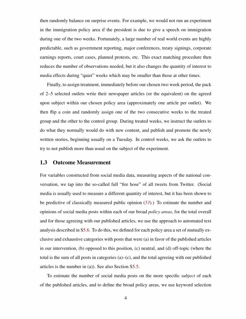
Figure S1 gives these results, with the p-value on the vertical axis, and the dashed

horizontal line marking α = 0.05, the point at or below which is conventionally referred

to as “statistically significant”. The simplest hypothesis tested here is at the left side of the

graph, for the effect of our randomized news media treatment on social media outcomes

during only first day following treatment (i.e., a test of γ1 = 0 in Equation 4). As we move

to the right, multiple days are included in joint tests (day 1, days 1 and 2, days 1 and 2

11

and 3,. . . ).

0.0

0.1

0.2

0.3

0.4

0.5

Days

Cla

ssic

al p

−va

lues

1 1−2 1−3 1−4 1−5 1−6

JointSubject

Policy

Agree

α = 0.05

Figure S1: Classic Hypothesis Tests for the causal effect of the news media (by, on thehorizontal axis, for days 1, 1 and 2, 1 and 2 and 3, etc.) on the number of social mediaposts about the specific subject of the treatment (“Subject”); the number of posts in thebroad policy area (“Policy”), a joint test of the two (“Joint”), and the proportion of postsagreeing with the position in the article in the broad policy area among those expressing anopinion (“Agree”). The α ≤ 0.05 significance region appears at and below the horizontallight gray dashed line.

By the design of our experiment, Figure S1 shows that the causal effects of our treat-

ment are significant at the α = 0.05 level for all combinations of days on the number of

social media posts in the specific subject area of the articles published (“Subject”, the blue

dashed line near the bottom), the number of social media posts in the broader policy area

(“Policy”, dark dashed blue line), and a joint test of policy and subject (“Joint”, in red).

For a concrete example of these categories, if we had an intervention about demonstra-

tions in support of the DREAM act, then “Subject” would include posts specifically about

protests about the DREAM act and “Policy” would include any posts regarding any topic

about immigration in general (even if not about the DREAM act).

We also measure the causal effect of our intervention on the percentage of (opinion-

ated) social media posts about a topic aligning with the opinions expressed in our treat-

12

ment articles (“Agree,” the top line in Figure S1). For our immigration example, “Agree”

would be the proportion of social media posts in the broad policy area of immigration that

are pro-immigration, among those expressing an opinion. We did not power our study to

detect precise effects for the causal effect on this variable and, as it turns out, this measure

is not significant in our data until all five or six days following treatment are considered

together in a joint test. The lack of day-by-day significance for this variable means that,

when we present our point estimates, we must be careful to not claim confident conclu-

sions about time trends in the causal effect of our experiments on it. However, even for

this variable, we will be able to detect an overall effect that is different from zero when

we consider the full experimental week.

2.4 Persuasive Effects on Expressed Opinion

Here, we estimate the persuasive effects of the media on the balance of opinion expressed

in social media posts within the policy area of our intervention. To estimate these effects,

we first determine the broad political or ideological position taken by each set of articles

published, which we do by reading the articles (in addition to knowing the journalists and

the outlets that joined each pack). We then estimate the percent of social media posts in the

same broad policy area taking a position on the same side of the issue. Our experimental

stopping rule was not designed to test the significance of this quantity of interest and so

we do not have results as precise as we might like. Nevertheless, as Figure S1 showed, the

stopping rule we used led us to collect enough data for a significant result when measuring

the joint effect over five or six days of social media posts.

The model-based causal effect point estimates, which appear in Figure S2, indicate

that, as a result of our intervention, opinion changes in the direction expressed in the

news media outlet articles by the end of the week by about 2.3 percentage points. In

other words, when the articles written by media outlets express a political opinion in their

writings, some Americans express themselves in ways consistent with this opinion and

others argue with the articles and express the opposite opinion, with the overall balance

of discussion in the national conversation tilting in favor of the opinions expressed in the

published articles as a result of our intervention. This figure shows that our intervention

13

increased discussion by both supporters and opponents of the opinion expressed by the

articles, with the balance of the increased discussion favoring the supporters. To be clear,

this estimated causal effect is not necessarily a change in the opinion of any one person (to

estimate that, we would need a research design at the individual level), but it is a change

in the balance of opinion among those who choose to express themselves as part of the

national conversation. The intervention thus changes the tenor of the national conversation

in ways that numerous other people will see and can potentially be influenced by.2

●

●

●

●

●

●

−2

0

2

4

Day 6

Day 5

Day 4

Day 3

Day 2

Day 1

Cha

nge

in N

umbe

r of

Pos

ts

●

●

●

●

●

●

●

●

●

●

●

●

Figure S2: Causal effect of news media on opinion expressed in the direction of thatexpressed in the news articles. Effects appear as the percentage point change in socialmedia posts for each day (●).

We did not collect enough data to be confident of the trend within the week in Figure

S2, and so the increasing effect we see in the model-based estimator (the red dots con-

nected with the line) on the balance of opinion as the week progresses requires further

research to confirm. The variation in the model-free estimates (the open circles) reflect

the appropriately higher level of uncertainty around the red dots and their trend, but even

with this variability five of the six of these estimates are above zero and they collectively

indicate a clear positive persuasive effect of the media on the overall composition of the2We do not include a total effect for this graph because adding the effects for each day would be mislead-

ing for this quantity of interest. For example, suppose a liberal intervention caused the balance of opinion inthe national conversation to be shifted in the liberal direction by two percentage points and to stay there forfour days. That effect seems better summarized in this way than saying that the “total” is eight percentagepoints since the balance was never greater than two.

14

national conversation.

2.5 Additional Observable Implications

We give results here for two additional observable implications of the causal effect of the

news media on the degree to which Americans express themselves publicly.

First, Figure S3 summarizes the causal effect represented in the sum of the first two

arrows in Figure 1 — the effect of our randomized treatment on website pageviews. We

estimated our causal effects, as usual, with our model-based (red dots) and model-free

(open circles) approaches but, unlike every other analysis in this paper, the results in this

figure imply some bias in the model-based estimates. This can be seen because all of

the open circles are at or above the red dots, rather than being approximately randomly

scattered around them, as in the other figures. As such, the true effect of the media on

pageviews is likely to be larger than that estimated by our model. The reason for the bias

in this unusual case is that a few of the observations for pageviews were unexpectedly

large values, in that they were not captured by our model. We thus add to this figure a

linear approximation fit to the open circles (see the gray dashed line). This third estimator

is the best linear approximation to the unbiased estimates, and its deviation from our first

model-based estimator represents the model bias from the skewed nature of the data.

On the scale of our estimates, the bias is small, and with or without the correction

added to the graph indicates a large effect of our randomized treatment on pageviews.

If we go with the (underestimated) model-based estimate, the treatment increased the

number of pageviews on the subject of our intervention on each day from 127% to 243%

per day, an overall increase over the week of 843% relative to a single day’s average

volume (left panel). These increases represent a total of 26,720 additional pageviews as

a result of our intervention (black square, right panel). (The upward trend in percent

increases in the left panel over time differ from the downward trend in the raw numbers

of pageviews in the right panel because the baseline volume of pageviews is usually lower

later in the week.) These substantial effects are consistent with, necessary for, and thus

observable implications of the large effects on public expression we estimate.

Second, we study in Figure S4 the causal effect of our randomized treatment assign-

15

●

●

●

●

●

●●

0

200

400

600

800

1000

1200

Tota

l Effe

ct

Day 6

Day 5

Day 4

Day 3

Day 2

Day 1

% C

hang

e in

Art

icle

Pag

evie

ws

● ● ●●

●

●●●

●

●

●

●

●

●

●

●●

●

●

0

10000

20000

30000

40000

50000

60000

Tota

l Effe

ct

Day 6

Day 5

Day 4

Day 3

Day 2

Day 1

Cha

nge

in A

rtic

le P

agev

iew

s

●● ● ● ● ●

●

●

●●

●

●

Figure S3: Causal effect of randomized treatment on news media outlet website pageviewsin percent change (left) and absolute numbers of posts (right), for each day (red dot, ●)and total overall (black square, ■).

ment on the number of social media posts in the specific subject area of the articles in

our intervention (even if not about articles that were part of the collaborating pack). The

causal effect estimate here provides a strong signal, with large effects, ranging from a

454% on the first day and dropping to 123% on day 6. Overall, this represents about

570 additional social media posts about these articles. Of course, the total effect of pub-

lishing the articles on the degree to which Americans express themselves is much larger

(as shown in Figure 2), and so clearly many of those caused to express themselves chose

to write only about the general policy area rather than this specific subject; some of the

posts about the broader policy area may also have been sparked by posts about the narrow

subject.

16

●

●

●

●

●

●

●

0

500

1000

1500

Tota

l Effe

ct

Day 6

Day 5

Day 4

Day 3

Day 2

Day 1

% C

hang

e in

Pos

ts

●

●

●

●●

●

●

●

●

●

●

●

●

●

●

●

●

●●

0

200

400

600

Tota

l Effe

ct

Day 6

Day 5

Day 4

Day 3

Day 2

Day 1

Cha

nge

in N

umbe

r of

Pos

ts

●

●

●

●●

●

●●

●

●

●

●

Figure S4: Causal effect of randomized treatment on the volume of social media posts onthe specific subject of the published articles, in percent change (left) and absolute numbersof posts (right), for each day (red dot, ●) and total overall (black square, ■).

3 Evaluating Sequential Hypothesis Testing

In this Section, we describe and extend techniques of sequential hypothesis testing, by re-

laxing assumptions and adapting them in ways that may have wider applicability beyond

this work. Although sequential hypothesis testing techniques have not often been used

in the social sciences, they seem to have great potential to lower the costs of data collec-

tion and increase the value of empirical results in many areas. We explain these points

here, with the hope that others may be able to take advantage. We now describe appropri-

ate sequential theories of inference, stopping rules, evaluation algorithms, and empirical

results.

3.1 Theories of Inference

The simplest statistical approach for a sequential experiment is within the likelihood or

Bayesian theories of inference, where novel statistical procedures are not required. In

other words, whether we collect an undifferentiated batch of n observations all at once or

we use interim results to decide when to stop collecting data, all likelihood-based infer-

17

ential procedures are still valid.3 Using these standard statistical methods for a sequential

experiment has the advantage of applying even when the real world intervenes and ends

the experiment earlier than expected or enables one to collect more data than planned.

Indeed, even multiple comparisons in testing is not an issue within appropriately modeled

Bayesian inferences. For these reasons, as well as for clarity and familiarity, we use use

this approach in Section S1.5.

In addition, because likelihood-based models with data-dependent stopping rules can

be sensitive to their (perhaps implicit) priors (69), we also go a step further and follow a

venerable procedure by evaluating a likelihood-based approach under frequentist theory,

using parametric and nonparametric evaluations.4

3.2 Stopping Rules

In the complicated real world for which our experiment was designed, our ability to collect

data at any point in time depends on numerous factors, such as the continued willingness

of the news outlets to continue to participate in our experiment, the value of collecting

as much data as possible, and whether we have at any point collected enough data to

draw reliable conclusions about specific quantities of interest. We also have a design with

several tests of direct interest and others as additional observable implications along the

causal pathway to be used to validate our results (as portrayed in Figure 1). For each, we

can test any combination of effects for groups of days of the week. However, by definition,

the number of experiments we run, and the final n, will be the same for all sequential

hypothesis tests and so we can only guarantee a chosen significance level for one or a

subset (an issue that also applies to power calculations in non-sequential frameworks).

For these reasons, relying solely on one formal stopping rule would be neither produc-

3Both theories of inference obey the “likelihood principle” (only that which is observed, and is thusreflected in the likelihood function, matters for inference), which in turns implies the “stopping rule prin-ciple” (the evidence provided through the likelihood function in a sequential experiment does not dependon the stopping rule) (67, Ch.7) or, in summary, likelihood inference is “invariant to sampling plans” (68,p.76ff). Technically, this assumes an ignorable stopping rule, meaning that all data are drawn from the samedistribution (or all information used in the stopping rule is available to the model) and the parameters of theprior and the stopping rule are a priori independent.

4Other types of frequentist sequential analysis have been developed, such as for confidence intervals,other measures of uncertainty, alternative experimental designs, and many other purposes (see 64, 70).

18

tive nor even in some circumstances possible. We thus combined (a) the recommendation

from a formal stopping rule, which we use as our primary quantitative guidance, along

with (b) the qualitative goal of collecting as much data as possible, the understanding that

data collection might at some point prove impossible earlier than desired or be continued

after we could have stopped based on (a), and a judgment based on the set of the con-

stellation of tests for each of our quantities of interest. From a formal likelihood point

of view, any way of using this information does not affect the statistical properties of the

tests or, as our frequentist evaluations below confirm, our conclusions.

The formal stopping rule we use for our primary quantitative guidance is the joint

hypothesis that the effect of the media in the first three days on social media posts in broad

policy areas and specific article subjects are significant at a p-value of 0.05. In addition,

for robustness, we make it more difficult than this to stop by also requiring significance

for some number of observations n, as well as at n − 1 and n − 2. So we start with 13

observations (experiments), test this joint hypothesis (on n = 13, 14, and 15), and then

sequentially add an observation, do a test, check this stopping rule, add an observation,

etc., until we reach significance on three in a row.

3.3 Evaluation Algorithms

Here, we explain our sequential hypothesis testing evaluation frameworks. Both the para-

metric and nonparametric procedures we introduce follow the same framework of gener-

ating 10,000 simulated data sets under the null hypothesis of no causal effect, and then

computing the false positive rate — the proportion of these data sets where we would be

led to conclude the causal effect is positive even though the true effect is zero.

Consider first this algorithm for generating one of these data sets (with details after-

wards for parametric and then nonparametric testing):

1. Set a starting value of N = 15 experiments

2. Generate a simulated data set with n = N observations following either parametric(in Section 3.3.1) or nonparametric (in Section 3.3.2) procedures.

3. Compute the p-value in the stopping rule described above and then:

(a) If p-value ≤ 0.05 stop (and conclude n = N is large enough to reject the null).

19

(b) If p-value > 0.05 and N < 35, set N = N + 1 and go to Step 2.

(c) If p-value > 0.05 and N = 35, stop.

The false positive rate is then the proportion of 10,000 data sets where the algorithm

stopped at Step 3 (a). (Step 3 could be continued to any number of observations, but we

stopped at 35 because the point of this algorithm is to evaluate the analysis we actually

ran.)

In practice, we modify this algorithm by using a more conservative sequential pro-

cedure that only allows one to stop collecting data only if we reach Step 3 (a) for three

consecutive numbers of observations (N − 2, N − 1, and N ). All that remains then is to

fill in Step 2 in this algorithm, the details for which we now do via the standard parametric

approach and our new nonparametric procedure.

3.3.1 Parametric Data Generation Process

Our first data generation procedure is based on the assumed distributions, using realistic

parameter values estimated from the data. It involves three steps, which we repeat n times

(i.e., for e = 1, . . . , n):

1. Randomly draw one policy area p = p′ from the 11 areas, distributed in the same

way as our 35 experiments.

2. For the treated week (Tped = 1), generate a week of outcome data {zpe1, . . . , zpe6}by drawing values from Model 2 using the estimated parameter estimates (and vari-ances), while restricting the treatment effect under the null to γd = 0.

3. For the control week (Tped = 0), also under the null, draw a week of outcome data{zpe1, . . . , zpe6} from the same distribution as the treated week.

Explicitly flipping coins to determine which week is treated and which is control is un-

necessary because, under the null, both are distributed in the same way, and the algorithm

draws the two weeks independently.

This standard parametric evaluation procedure provides a useful evaluation of our

sequential hypothesis testing framework, but it has a weakness in that it assumes the

veracity of our estimation framework. Since the systematic component of model 2 is very

nearly nonparametric (i.e., except for the assumption that the 6 daily parameters can be

20

reduced to 2), the primary modeling assumption in generating the simulated data is the

normal stochastic component. We now show how to remove this assumption.

3.3.2 Nonparametric Data Generation Process

To draw data under the null without a normal distribution assumption, we use the ac-

tual social media data measurements for our experiments in control weeks and randomly

assign them to pseudo-treatment and control conditions (with no actual intervention). Al-

though this procedure is designed especially for and close to our actual experiments, so

that it is highly realistic, it is also fairly generic and appears applicable to many other

sequential hypothesis testing applications.

We begin with all streams of social media measures, zped, for policy area p (p =

1, . . . , 11), day d (d = 1, . . . , 6). We then generate an experiment under the null e for any

sequential pair of weeks during our observation period as follows:

1. Randomly select a publication day (usually a Tuesday) between 9/2014 and 3/2016(the time during which we ran our experiments) with no major predicted events inpolicy area p′.

2. Apply rejection sampling: If any day during the two weeks following the selectedpublication day overlap with an actual experiment we ran in policy area p, discardit and go to Step 1.

3. Assign treatment to the two (matched) weeks by flipping one fair coin, with headsindicating that the first week is treated and the second control, and tails indicatingthe reverse.

This procedure then leaves us with a data set generated from control weeks that could

have been chosen for random treatment intervention, but were not. We then use both the

standard parametric approach, and this new nonparametric (or “placebo”) approach, to

generate 10,000 simulated data sets. With these, we compute and report false positive

rates to evaluate our sequential hypothesis testing framework.

3.4 Empirical Results

We now evaluate the classical hypothesis tests in Figure S1 in the context of sequential

stopping rules under a frequentist theory of inference. We do this in several ways, which

21

differ by the assumptions necessary for estimation and for simulation. For estimation,

the left panel in Figure S5 uses our model-based estimator, the linear regression model

in Equation 2, whereas the right panel uses our model-free estimator, the difference-in-

means, where the units of analysis and treatment are the same, thus eliminating the linear-

ity, normality, and conditional time series independence assumptions of the model-based

approach. For simulation within each panel (i.e., for each estimator), we generate data

under the null in two ways, first drawing in a standard way from the parametric model in

Equation 2 (labeled “P”) and then using a fully nonparametric approach, which makes no

modeling or independence assumptions at all (“NP”). The parametric simulation method

assumes Model 2, whereas the nonparametric method eliminates the linearity and normal-

ity assumptions. In both panels, the horizontal axes are the same as in Figure S1, while

the vertical axis is the sequential analysis false positive rate (the proportion of simulated

data sets where the stopping rule indicated that we should stop collecting observations

but where we would have incorrectly concluded there was an effect). Both panels were

constructed using a stopping rule, as we did in practice, requiring statistically significant

results for three consecutive tests, of n, n − 1, and n − 2.

0.0

0.1

0.2

0.3

0.4

0.5

Days

Pro

port

ion

Fals

e P

ositi

ves

1 1−2 1−3 1−4 1−5 1−6

●

●

●

● ●

●

Agree NP

Policy NP

Subject NP

Joint NP

Agree P Policy P Subject P

Joint P

α = 0.05

0.0

0.1

0.2

0.3

0.4

0.5

Days

Pro

port

ion

Fals

e P

ositi

ves

1 1−2 1−3 1−4 1−5 1−6

●

●● ● ● ●

Agree NP

Policy NP

Subject NPJoint NP

Agree P Policy P Subject P

Joint P

α = 0.05

Figure S5: False Positive Rates from parametric (“P”) and nonparametric (“NP”) simula-tions for a stopping rule composed of three consecutive significant tests. Other symbols,and the horizontal axis, follow Figure S1. The left panel is based on the model in Equation2 with 6× 35× 2 = 420 observations, whereas the right panel is calculated from a simpledifference in means (with 35 observations in each group).

22

The key result in this figure is that both joint tests (for P and NP), for each combination

of days and tests, and for the model-based estimate in the left panel and the difference of

means estimator in the right panel, are significant at 0.05 (see black and red lines at the

bottom of the left panel). This confirms the classical hypothesis testing result as a stopping

rule. Tests for some individual results at the left of each panel indicate more uncertainty

than the classical test and so suggest more caution in interpreting the corresponding in-

dividual point estimates we describe in the text. Yet, by the time we are evaluating the

effect of the intervention on five or six days in the test (at the right of each panel), the

stopping rule is significant for every variable. This panel also shows that the nonpara-

metric tests are larger for most, but not all, variables than their corresponding parametric

tests, but with no marked substantive differences between the two overall. (Estimates from

the difference-in-means estimator have higher variances than the model-based approach,

which also means that stopping is more difficult and so false positives are less likely as

well under the null.)

4 Evaluating Heterogeneous Effects

4.1 Leave-One-Outlet-Out Jackknife Estimation

Given the heterogeneity in the size and audience of the outlets participating in our study,

one question is whether the results we find are attributable to one large media outlet or an

outlet that for some chance reason happened to have a particularly large effect. Taking any

subset of data for a revised estimate, especially based on outcome variable measurement,

would generate post-treatment bias. However, we can study this question by taking all

possible subsets without regard to the outcome and studying them as a set. We thus use a

jackknife procedure, that also has the advantage of computing another set of uncertainty

estimates for our main causal effects.

Our version of jackknife estimation is a “leave-one-outlet-out” estimation procedure,

in which we identify all the experiments that a given outlet participated in and then omit

those experiments when calculating treatment effects. We then repeat this procedure for

each outlet in turn. In total, 33 outlets participated in the 35 experiments in which we

23

implemented our final experimental protocol (the remaining outlets participated in pilot

experiments that helped us hone our approach). For each dataset resulting from dropping

an outlet, we plot daily treatment effects calculated as in Figure 2 in our paper. These

can then be compared to the treatment effects when using the full sample of outlets (es-

timates denoted by red circles). Figure S6 presents the results of this procedure for our

primary outcome variable, i.e., the number of broad policy Twitter posts resulting from an

experimental intervention.

●

●

●

●

●

●

0

2000

4000

6000

Day 6

Day 5

Day 4

Day 3

Day 2

Day 1

Cha

nge

in N

umbe

r of

Pos

ts

●

●

●

●

●

●

●

●

●

●

●

●

●

●

●

●

●

●

●

●

●

●

●

●

●

●

●

●

●

●

●

●

●

●

●

●

●

●

●

●

●

●

●

●

●

●

●

●

●

●

●

●

●

●

●

●

●

●

●

●

●

●

●

●

●

●

●

●

●

●

●

●

●

●

●

●

●

●

●

●

●

●

●

●

●

●

●

●

●

●

●

●

●

●

●

●

●

●

●

●

●

●

●

●

●

●

●

●

●

●

●

●

●

●

●

●

●

●

●

●

●

●

●

●

●

●

●

●

●

●

●

●

●

●

●

●

●

●

●

●

●

●

●

●

●

●

●

●

●

●

●

●

●

●

●

●

●

●

●

●

●

●

●

●

●

●

●

●

●

●

●

●

●

●

●

●

●

●

●

●

●

●

●

●

●

●

●

●

●

●

●

●

●

●

●

●

●

●

●

●

●

●

●

●

Figure S6: “Leave one outlet out” when estimating causal effect of news media on publicexpression, denominated in absolute change in numbers of social media posts in a broadpolicy area. The full results are represented by our model-based estimator, ●, and theleave-one-out estimates, ◦.

The figure demonstrates that omitting any one outlet does not meaningfully change

the results of the experiment. Especially in the first three days after an intervention, we

continue to find large, positive point estimates no matter which outlet we omit from the

estimation procedure.

24

4.2 Treatment in Week One versus Week Two

Another issue is how the structure of the experiment—particularly, that we used paired

weeks with the treatment week directly following the control week or vice versa—affected

our results. One issue is spillover from the first to the second week. Another possibility

could be that when the collaboration occurs in week one outlets are more likely to for-

get they are involved in an experiment in week two and therefore continue to publish

or promote on-topic articles in the second week. Similarly, when the treatment week is

randomly selected to be the second of the two weeks, outlets might do less to keep their

coverage “quiet” in the topic area of the experiment in the first week, which is supposed

to serve as a control week. Any of these issues might affect our estimates; however, each

would actually bias our effect sizes downwards, and we would likely be understating the

true effect since in each case readership and social media posts in the control week would

be higher than in the case of perfect compliance.

Nonetheless, to test these accounts, we create an indicator variable for each experiment

that encodes whether treatment occurred in week one or in week two. We then fully

interact that variable with the other variables relevant to calculating treatment. To test

whether timing of the experiment (in week one or week two) mattered, we examine the

interaction of this variable with the treatment variables. We find that there is a slightly

larger treatment effect when treatment occurs in the second week, but a hypothesis test

where the null is that there is no difference in treatment effects depending on whether

treatment occurs in week one or two cannot be rejected (β̂ = −0.197 and se(β̂) = 0.189).

Taking another approach, when subsetting the data into two separate groups depending

on week one or week two treatment, a point estimate on the log scale for day one is 0.093

when treatment occurs in week one versus 0.289 when treatment occurs in week two.

Our conclusion is that there is not sufficient evidence to conclude definitively that

there is a meaningful difference depending on in which week the treatment occurs. The

levels of both are positive (and large) and we find no statistically significant difference

between the two. And any undetectable bias which might exist is likely to reduce the size

of our reported effects.

25

4.3 Variation in Effects by Experiment

Another natural question is the size of effects across experiments. We show there is the

expected heterogeneity; indeed, with our sequential design, this is the major factor lead-

ing us to have to collect as much data as we did. Because discussion on social media

is “bursty” and generally high variance, there is considerable heterogeneity in the effects

across experiments. To illustrate this heterogeneity, for each experiment (N = 35), we

paired each day of the week from the treatment week with each day from the control week.

Then, for each day, we calculated the difference of our measure of broad policy discus-

sions on social media (log-transformed, as in the rest of the paper). Table S1 illustrates

the results.

Table S1: Heterogeneous effects, Summary of effects by experiment and day of week

Min. 1st Qu. Median Mean 3rd Qu. Max.Day 1 -1.252 -0.171 0.053 0.207 0.245 2.342Day 2 -1.087 -0.074 0.110 0.160 0.415 1.458Day 3 -1.645 -0.045 0.111 0.014 0.259 0.669Day 4 -1.049 -0.194 0.024 0.052 0.344 0.902Day 5 -1.211 -0.239 0.081 0.138 0.334 2.644Day 6 -3.014 -0.319 0.026 -0.022 0.353 1.674

As the table illustrates, there are certainly cases where some of the individual causal

effects are negative for each day of the week, and there were even some cases of extreme

negative outliers on a daily basis. However, a significant majority of daily effects were

positive (as one would expect given our regression results). For instance, the median effect

is positive across all days and it ranges in size from 0.111 to 0.024 depending on the day

and typically over 60% of all individual daily effects were positive as compared to the

same day in the control week, with the exception of the sixth (last) day of the experiment.

26

5 Social Media Posts as an Outcome Variable

5.1 Composition of Social Media Posts5.1.1 Political Content on Twitter

Discussion of political events and policy issues on Twitter is small compared to other

types of discussion, like entertainment or sports, but it appears important in and of itself.

As we note in the main text, there are generally fewer tweets about immigration in a given

week than there are about the television shows Scandal or the Bachelor. Nevertheless,

Twitter users do talk about political issues regularly. Pew’s 2015 study of a representative

sample of American Twitter users found that about half of Twitter users post about “news”

(including entertainment and other current events) at least once in the month examined,

and that about 17% of those news-focused tweets are about “government & politics” (71).

Further, although many Twitter users do not post about politics (in a 2016 Pew survey,

60% of users reported that “none” of what they post is about politics), users do view

political discussion on Twitter as meaningful and important. Pew reports that most social

media users (including Twitter users) think that social media “helps users get involved

with issues that matter to them,” and one in five of them report they have modified their

views about a political or social issue because of something they saw on social media (72).

5.1.2 Social Media Post Authorship

One might worry that political Twitter posts are produced by bots, or other news outlets

retweeting news stories. (Of course, bots and news outlets are also generated by humans,

although one step removed and potentially in numbers larger than they could as individu-

als.) To study this issue, we manually coded a sample of posts.

We and our research assistants hand-coded 200 randomly-sampled posts (100 drawn

from tweets that fell into our topic categories during “treatment” weeks, and 100 from

“control” weeks). We examined each user’s Twitter handle on the Twitter site (e.g.

https://twitter.com/POTUS) and tried to assess whether that user was (1) a

bot, (2) an individual person, or a group/organization of some kind, or (3) a journalist

or news organization. Some users (20 of the 200 posts coded) could not be evaluated

27

because their Twitter accounts were made private or had been deactivated or suspended

since we collected our data. We also checked the first 50 codings of “bot or not” against

the online tool “Botometer,” which attempts to automate the detection of Twitter bots

(https://botometer.iuni.iu.edu/), and found only 3 disagreements. We then

manually checked those three accounts and determined that two of them were indeed bots

(in our judgment), and the third account was unclear. This procedure assures us that our

hand coding of bots is quite reliable.

Overall, we found relatively few bots in our sample of posts: we identified 28 posts by

bots out of our 200-tweet sample. And more importantly, they occurred at the same rates

during treatment and control weeks. We also found relatively few posts by journalists or

news outlets (as inferred from usernames and profile bios): 21/200 posts appeared to be

from journalists or news organizations (10 treatment week, 11 control). None of these

posts by journalists/news outlets were from any of the outlets that participated in our

study. We found that about 80% of accounts appeared to be owned by individuals.

We used string operations to identify retweets, and a substantial fraction (90/200) of

the sampled posts are indeed retweets. However, research on Twitter dynamics suggests

that retweeting another user’s post is a meaningful action and should be interpreted as

a political behavior, just as someone by the water cooler asking “Did you see that New

York Times editorial about the president?” or responding to someone else’s point “Yeah,

I agree” should be interpreted as a meaningful contribution to democratic discourse. Liu,

Kliman-Silver, and Mislove (73) reports an increase in retweeting behavior on Twitter

over time, while Recuero, Araujo, and Zago (74) reports that the most common rea-

sons users gave for retweeting posts were to “Share relevant information with followers,”

“Show agreement,” and “Show support.” Further, a Pew study of political behavior on

Twitter found that the majority of news-related Twitter activity was retweets (71). The lit-

erature suggests that retweeting is a common and meaningful Twitter behavior that should

be considered part of policy discussions on Twitter.

28

5.2 Measuring Twitter User Characteristics

Figure 3 reports treatment effects among various subgroups on Twitter: gender, region,

influence, and political affiliations. Here, we discuss the process by which these users are

identified and limitations of our approach.

Our Twitter data was provided by the firm Crimson Hexagon, and we rely on their

classification of Twitter users as well. To predict users’ gender, Crimson Hexagon relies

on name classification. They pull users’ self-reported first names from their profiles, and

use the gender distribution of names in census data and other public records as inputs to

predict the gender of each user from their name. These are well known procedures in the

academic literature.

To predict users’ states in the US (which we then aggregated up into Census regions),

Crimson Hexagon relies on a combination of user-provided latitude-longitude information

(geotagging of posts) and other information from users’ posts and profiles, such as the

“location” field and users’ time zones.

The “influence” measure we use here are Klout scores, which run 0–100. They are pro-

prietary scores (by Lithium, Inc.) described at https://klout.com/corp/score.

Briefly, they aim to measure how many different people interact with a user’s posts across

several social media platforms; they are based mostly on followers and the social graph.

Our own detailed analyses of this question show that numerous measures of influence in

social media differ but tend to be highly correlated.

Our measure of political affiliation relies on Crimson Hexagon’s “affinities” measures.

These measures attempt to classify users as having an affinity for a range of topics (rock

music, travel, the Democratic Party) based on their tweets and the users they follow. For

this project, we rely on Crimson Hexagon’s estimate of users as having affinities for the

Republican or Democratic parties. Although most Twitter users are not classified as hav-

ing an observable affinity for either party, this measure should give us a sense of whether

users that express themselves as having a partisan preference are generally Republican-

or Democratic-leaning.

Our analyses show that the causal effects of our intervention do not differ significantly

29

across these subgroups. We encourage future researchers to carry out interventions where

more detailed characterizations of individuals is possible so that we can rule out aggregate

uniformity masking sub-aggregate differences.

5.3 Logged Outcome Variable

All social media data is notoriously “bursty” and tends towards having high variance due

to the existence of outliers when a topic of discussion is picked up widely. As a result,

using social media data as the outcome can lead to having an outcome variable with a

substantial right-skew. This is the case in our data too and so, throughout, we perform a

simple transformation on the outcome variable by taking the natural log of the outcome

variable plus one-half (i.e., ln(y + 1/2)).

When we do not log transform the data, we find — exactly as expected — that esti-

mates are less efficient, comparable in magnitude but with higher variance. These noisier

results are common when analyzing a highly skewed variable due to the larger influence

of outliers (which can occur in both treatment and control weeks).

5.4 Choosing Policy Areas and Keywords5.4.1 Policy Areas

To choose the policy areas to conduct the experiments, we engaged in lengthy discussions

with participating outlets. With their input, we settled on topic areas that the participating

outlets were willing and excited to cover on the one hand, and that appeared relevant to

existing national conversations about public policy on the other hand. In addition, we

sought topics that would lend themselves to “evergreen” articles (i.e., articles not overly

time-sensitive or involving breaking news). The general definitions of the 11 policy areas

in our experiment are listed in our paper (in some cases slightly modified to ensure each

outlet publication is not identifiable). We now describe how we came up with operational

definitions for each.

30

5.4.2 Keywords

To identify the set of social media posts about a given policy area, we generated a list of

keywords as follows:

1. We begin with a limited set of keywords (generally just a few words) as a search

term to discover an initial set of social media posts on a given policy topic. For

example, use the search string (immigration OR immigrant) to begin to

unearth posts on the policy area of Immigration.

2. Perform two parallel processes to add keywords to our list

(a) Qualitative Approach

i. Read posts unearthed on a given topic to develop potential additional key-

words. Here, the key judgment is determining what additional keywords

characterize the topic under consideration while also insuring that they do

not pull in a large share of unrelated or off-topic social media posts.

ii. Respecify the set of keywords to incorporate the new terms, perform a

new search, and repeat the process of discovering new posts and distilling

new key words from these posts. Perhaps the best analogy is snowball

sampling, but in the realm of keyword discovery.

(b) Algorithmic Approach

i. Apply the keyword generation procedure described in King, Lam, and

Roberts (54) to generate additional potential keywords. In brief, when

adding a new set of posts, run this algorithm on a random sample of posts

drawn from the existing body of posts pooled with the newly discovered

posts. The model is trained based on which posts are in the existing set

of posts and which set are in the newly added set. Then fit the model on

the remaining newly added posts to identify posts that are similar to those

from the existing set of posts. Extract new, relevant keywords from these

newly identified “on-topic” posts based on how frequently the keywords

31

are used in the newly identified posts. The main feature of the algorithm

is that it learns from, rather than correcting, mistakes in classifying posts

as relevant and mines keywords from those mistakes.

(c) After generating lists of candidate keywords, we then selected a final set of

keywords based on the pool of keywords generated from the methods de-

scribed above.

5.5 Coder Training Procedures

We enlisted a team of research assistants to label documents for our training sets. Each

coder received the following training. For each categorization, we randomly selected

several hundred social media posts from our database of all posts. Then, at least one and

often two of the principal investigators independently labeled these posts. The coder being

trained then was given the task of coding the posts, independently. We then compared

the human coders’ decisions to those made by the principal investigators and discussed

points of difference. We then repeated this process (with a new set of social media posts)

until the level of agreement reached acceptable levels, almost always well above 70%

and, more importantly, the confusion matrix did not reveal any systematic error patterns

that might have biased any results in favor of one category or another. At this point, we

had our research assistants code approximately 1,000 posts in each policy area, with any

disagreements broken by discussion among the assistants or by us (so that no posts had

detectable coding errors). As the total number of posts needed to achieve a certain level

of confidence depends on the entropy in the number of posts across categories, we took

advantage of a feature of our text analytic approach (see Section S5.6) that allows us to

be guided in our decision about when to stop coding by an adaptive methodology that

requires more coding when there happens to be large imbalances in posts across the four

categories.

5.6 Automated Text Analysis Procedures

The text analytic methods we used are described in (18, 75, 76). They are known as

“readme,” after the open source software that implements it (77). The papers give an in

32

depth description of the method; here, we give some intuition for how the method works.

Consider a set of n social media posts, each of which falls into one of k mutually

exclusive and exhaustive categories Di ∈ {1, . . . , k} (for i = 1, . . . , n). For example, in

the policy area of Immigration, the categories could be (1) Pro-Immigration/Sympathetic

to Immigrants/In Favor of More Immigration; (2) Anti-Immigration; (3) Neutral on Im-

migration; and, to ensure the categories are exhaustive, (4) Off-Topic.

Then draw a random sample of posts and label them via the coding procedures de-

scribed in Section S5.5. Denote this as the labeled set and the remaining social media

posts the unlabeled set. The quantity of interest is P (D)U , a k× 1 vector of category pro-

portions falling on the simplex. To estimate P (D)U we use as inputs the textual content

of all the social media posts in both sets.

Automated text analytic methods typically work in two steps: turning the text into

numbers and then analyzing the numbers via statistical methods. As a simple version of

how text can be summarized, take the text, stem all the words (so consist, consistency,

and consisted are all summarized as consist), make them all lower case, and remove all

punctuation. Suppose we find w unique word stems in the entire corpus. Then summarize

each post as a word stem profile — a w × 1 vector of ones and zeros, representing the

presence or absence respectively of every unique word stem, with 2w possible word stem

profiles.

Define P (S)U as a w × 1 frequency distribution of the proportion of social media

posts that fall within each of the possible word stem profiles for the unlabeled set. Denote

P (S∣D)U as aw×k matrix, each column of which is a word stem profile frequency distri-

bution for one category in the unlabeled set. Then by definition, the following expression

is an accounting identity; that is, it holds exactly, without an error term:

P (S)U = P (S∣D)UP (D). (5)

In addition, P (S)U is directly observed by tabulating the test set. Since the labeled set

is randomly sampled from the same source as the test set we can get P (S∣D)U from the

equivalent in the labeled set by assuming in expectation that E[P (S∣D)U] = P (S∣D)L.

33

If we then use this expression, substitute in, and solve for the quantity of interest, we get

P (D)U = [P (S∣D)L′P (S∣D)L]P (S∣D)L′P (S)U , which shows that we can estimate

the unlabeled set category proportions without any method of individual classification.

The actual method uses more sophisticated methods of summarizing text, constrained

regression to keep the outcome to the simplex, simplifications because 2w is large and

mostly empty, and several other computational techniques for speed and accuracy. When

the labeled set is not a random sample from the test set, the appropriateness of the key

substitution above can be maintained by adding documents to the labeled set over time as

data are collected.

6 Experimental Interventions

6.1 Comparison between Normal and Treatment Articles

Here we study how representative our treatment outlets were of articles the outlets nor-

mally publish. We tried to ensure they would be representative by working hard to ensure

that the outlets followed the same procedures they do in the normal course of their jobs.

The goal for our intervention articles was to be representative of the set of articles the

media outlets write within our eleven policy areas, on topics of national importance, of

interest to journalists, and which could be held and published over the subsequent two

weeks rather than immediately.

We compared the two qualitatively during our years of trial runs and then in ongoing

monitoring as we ran the experiments. In addition, we also offer here a more systematic

comparison of an analysis of our published articles to the set of all articles published by

these outlets. This is not the ideal comparison set from the point of view of representa-

tiveness — since it includes minor public interest stories, articles about urgent breaking

news, stories outside of our eleven policy areas, etc. — but it gives a sense of how our

articles fit within the set of all articles published by these outlets.

We study this question by using all available data, comparing on-topic treatment week

articles (the ones that constitute our experimental treatment) and the full corpus of pub-

lished articles from the 18 months of our study (with some measurement error for tech-

34

nical reasons resulting in truncation of some non-treatment articles). For each individual

outlet (because our outlets differ quite a bit in their publishing styles), we calculate the

mean word length of all articles and of treatment articles, as well as the mean reading

level (Flesch-Kincaid grade level) of each type of article. Then we subtract the “normal”

article scores from the “treatment” article scores to get a sense of how much the treatment

articles differ from the full corpus. We present our results in Figure S7. In the right panel,

we present word count differences: each circle represents one outlet’s mean difference in

article length between the full corpus and the treatment articles. There is substantial vari-

ation, with some outlets publishing longer articles than usual as part of the treatment, and

a few publishing shorter ones. The median outlet has a (mean) word count difference of

−369, indicating that their treatment articles were typically longer than their usual articles.

Similarly, the left panel presents grade-level differences. A number of outlets have pos-

itive values, indicating that their regular articles were more complex than their treatment

articles, and others have negative values. The median difference is less than half a grade

level, which is substantively quite small. Some (though not all) outlets may have been

publishing slightly longer articles as part of the experiment, but they were not publishing

substantially more complex ones. On the whole, we think it reasonable to conclude that

our results should generalize relatively well to these outlets’ typical content.

Qualitatively, the articles published as part of this study cover the range of content usu-

ally published by these outlets. Some pieces included substantial investigative reporting,

others were feature pieces, others were opinion or news commentary pieces without orig-

inal reporting. We expected this heterogeneity, and that it would add to the n necessary to

stop according to our sequential hypothesis testing procedures.

6.2 Checking for News Shocks

Our study involved randomizing the publication date of news articles, so our estimates of

the effects of publication are unbiased. Whether some major news event happened during

one of our experiments is irrelevant in expectation, as random noise will occur evenly

across our treatment and control weeks. But we still might ask whether conditional on

our sample our results might have been due to luck. In this section, we explore this

35

●

●

●

●

●

●

●

●

●

●

●●

−3

−2

−1

01

2

Grade Level Differences, Experimental/Regular Articles

Fle

sch−

Kin

caid

Gra

de−

Leve

l Diff

eren

ce (

by O

utle

t)

●

●●●

●

●

●

●

●

●

●

●

−20

00−

1500

−10

00−

500

050

0

Word Count Differences, Experimental/Regular Articles

Wor

d C

ount

Diff

eren

ce (

by O

utle

t)

Figure S7: Comparing treatment articles to outlets’ usual content

possibility using data on local nightly news broadcasts.

We draw news story overviews from the Tyndall Report (tyndallreport.com),

which tracks all news stories covered by the three major networks’ weeknight news broad-

casts. Their online search page contains story overviews from 2006 to mid-September

2015; this time period covers a substantial part of our experimental period, and allows us

to draw data that covers the two-week experimental periods for 18 of our interventions.

We merged all the downloaded nightly-news-story overviews with our experimental data,

such that each of those 18 experiments was matched to all of the nightly news stories that

ran during that two-week period. This resulted in a set of about 4000 nightly news stories

36

to code (some individual stories were repeated, since they fell during multiple experiments

on different topics).

We then manually coded these stories based on the brief descriptions of them given

by the Tyndall Report, to see whether they were on the same subject as the experiment

taking place during that time (i.e. during an experiment we ran about immigration, were

there nightly-news stories about immigration being run?). We did this coding while blind

to treatment status of any given week.

The resulting codings suggest that, for the 18 experiments we were able to compare

to nightly-news data, there were no major news spikes that likely drove our results, and

the “quiet” pairs of weeks we choose for our experiments were indeed relatively quiet.

Of the 36 weeks we were able to study here (18 treatment and 18 control), a total of

11 saw some sort of on-topic nightly-news coverage, with 5 in control and 6 in treatment.

There were a total of 29 nightly-news articles on our broad experimental topics, 12 control

and 17 treatment, and a t-test cannot reject the null of no difference in the proportion of

nightly news articles that were about experimental topics during control and treatment

weeks (.006 versus .008). This result is of course as expected given the random treatment

assignment.

6.3 Outlet Audience Size

Precise measures of overall internet traffic are difficult to come by, particularly for small

sites. We used data from Google Analytics accounts from the outlets that provided it to us.

For others, we estimate overall audience sizes for these sites using data from Alexa site

rankings. Alexa’s data allows us to look at sites’ “Alexa ranking” (their estimate of how

prominent the site was compared to other sites on the internet at the time, with Google

ranked as 1, Youtube 2, Facebook 3, etc.) through time, and also generates estimates of

monthly unique visitors and total pageviews for the last month. We collected these data

in mid-2017, so our estimates of web traffic may not correspond perfectly to our 2014–

2016 experiments. We note that this measure of “audience” relies entirely on web traffic

to the site, and will underestimate the reach of those of our outlets that also publish print

editions, radio broadcasts, or distribute information in other ways. We also have to assume

37

that sites not ranked by Alexa are smaller than the ones ranked.

We collected Alexa data for the 33 outlets that participated in our final experimental

design; these are the outlets that generated the data used in the paper, so it is most impor-

tant to understand their characteristics (as opposed to the full set of outlets that helped us

develop the experimental protocol and granted us Google Analytics and other data). Alexa

only generates estimates of pageviews and unique visitors for the top sites on the internet.

About half of our outlets fall below this threshold, so we do not have estimates of their web

traffic. The remaining 18, for which we have Alexa estimates, range from almost 30,000

to about 1.5 million unique visitors per month. Estimated monthly pageviews range from

200,000 to 13 million, with the median site getting about 2.2 million pageviews per month.

38

References

1. J. T. Klapper, The Effects of Mass Communication (Free Press, 1960).

2. L. Guo, M. E. McCombs, The Power of Information Networks: New Directions for Agenda

Setting (Routledge, 2015).

3. M. E. McCombs, D. L. Shaw, The agenda-setting function of mass media. Public Opin. Q. 36,

176–187 (1972). doi:10.1086/267990

4. J. R. Zaller, The Nature and Origins of Mass Opinion (Cambridge Univ. Press, 1992).

5. M. A. Baum, T. Groeling, New media and the polarization of American political discourse.

Polit. Commun. 25, 345–365 (2008). doi:10.1080/10584600802426965

6. S. Iyengar, D. R. Kinder, News that Matters: Television and American Opinion (Univ. of

Chicago Press, 2010).

7. T. E. Nelson, in The Oxford Handbook of American Public Opinion and the Media, G. C.

Edwards III, L. R. Jacobs, R. Y. Shapiro, Eds. (Oxford Univ. Press, 2011), pp. 156–168.

8. W. L. Bennett, S. Iyengar, A new era of minimal effects? The changing foundations of

political communication. J. Commun. 58, 707–731 (2008). doi:10.1111/j.1460-

2466.2008.00410.x

9. W. A. Gamson, Talking Politics (Cambridge Univ. Press, 1992).

10. J. G. Gunnell, in The Oxford Handbook of American Public Opinion and the Media, G. C.

Edwards III, L. R. Jacobs, R. Y. Shapiro, Eds. (Oxford Univ. Press, 2011), pp. 1–18.

11. P. M. Kellstedt, The Mass Media and the Dynamics of American Racial Attitudes

(Cambridge Univ. Press, 2003).

12. D. Carpenter, C. D. Moore, When canvassers became activists: Antislavery petitioning and

the political mobilization of American women. Am. Polit. Sci. Rev. 108, 479–498 (2014).

doi:10.1017/S000305541400029X

13. B. Manin, The Principles of Representative Government (Cambridge Univ. Press, 1997).

14. G. King, J. Pan, M. E. Roberts, How censorship in China allows government criticism but

silences collective expression. Am. Polit. Sci. Rev. 107, 326–343 (2013).

doi:10.1017/S0003055413000014

15. G. King, J. Pan, M. E. Roberts, Reverse-engineering censorship in China: Randomized

experimentation and participant observation. Science 345, 1251722 (2014).

doi:10.1126/science.1251722 Medline

16. J. Fishkin, Election Law J. 12, 490–507 (2013).

17. L. M. Sanders, Against deliberation. Polit. Theory 25, 347–376 (1997).

doi:10.1177/0090591797025003002

18. D. Hopkins, G. King, A method of automated nonparametric content analysis for social

science. Am. J. Polit. Sci. 54, 229–247 (2010). doi:10.1111/j.1540-5907.2009.00428.x

19. S. Verba, K. L. Schlozman, H. E. Brady, Voice and Equality: Civic Volunteerism in

American Politics (Harvard Univ. Press, 1995).

20. M. A. Baum, Soft News Goes to War: Public Opinion and American Foreign Policy in the

New Media Age (Princeton Univ. Press, 2003).

21. L. M. Bartels, Messages received: The political impact of media exposure. Am. Polit. Sci.

Rev. 87, 267–285 (1993). doi:10.2307/2939040

22. L. Vavreck, S. Iyengar, in The Oxford Handbook of American Public Opinion and the Media,

G. C. Edwards III, L. R. Jacobs, R. Y. Shapiro, Eds. (Oxford Univ. Press, 2011), pp. 156–

168.

23. L. Vavreck, The exaggerated effects of advertising on turnout: The dangers of self-reports.

Q. J. Polit. Sci. 2, 325–343 (2007). doi:10.1561/100.00006005

24. M. Prior, Improving media effects research through better measurement of news exposure. J.

Polit. 71, 893–908 (2009). doi:10.1017/S0022381609090781

25. R. R. Bhavnani, G. Nellis, Can Government-Controlled Media Cause Social Change?

Television and Fertility in India (Univ. of Wisconsin, 2016); http://j.mp/2yIeZoL.

26. S. DellaVigna, E. L. Ferrara, Economic and Social Impacts of the Media (National Bureau of

Economic Research, 2015); http://j.mp/2yIkiVd.

27. S. DellaVigna, E. Kaplan, The Fox News effect: Media bias and voting. Q. J. Econ. 122,

1187–1234 (2007). doi:10.1162/qjec.122.3.1187

28. M. Gentzkow, J. M. Shapiro, M. Sinkinson, The effect of newspaper entry and exit on

electoral politics. Am. Econ. Rev. 101, 2980–3018 (2011). doi:10.1257/aer.101.7.2980

29. M. Gentzkow, Television and voter turnout. Q. J. Econ. 121, 931–972 (2006).

doi:10.1162/qjec.121.3.931

30. G. A. Huber, K. Arceneaux, Identifying the persuasive effects of presidential advertising.

Am. J. Polit. Sci. 51, 957–977 (2007). doi:10.1111/j.1540-5907.2007.00291.x

31. A. Reeves, M. McKee, D. Stuckler, ‘It’s the Sun wot won it’: Evidence of media influence

on political attitudes and voting from a UK quasi-natural experiment. Soc. Sci. Res. 56,

44–57 (2016). doi:10.1016/j.ssresearch.2015.11.002 Medline

32. G. Smith, K. Searles, Who let the (attack) dogs out? New evidence for partisan media effects.

Public Opin. Q. 78, 71–99 (2014). doi:10.1093/poq/nft082

33. J. Conroy-Krutz, D. C. Moehler, Moderation from bias: A field experiment on partisan media

in a new democracy. J. Polit. 77, 575–587 (2015). doi:10.1086/680187

34. A. S. Gerber, D. Karlan, D. Bergan, Does the media matter? A field experiment measuring

the effect of newspapers on voting behavior and political opinions. Am. Econ. J. Appl.

Econ. 1, 35–52 (2009). doi:10.1257/app.1.2.35

35. D. P. Green, B. R. Calfano, P. M. Aronow, Field experimental designs for the study of media

effects. Polit. Commun. 31, 168–180 (2014). doi:10.1080/10584609.2013.828142

36. D. P. Green, L. Vavreck, Analysis of cluster-randomized experiments: A comparison of

alternative estimation approaches. Polit. Anal. 16, 138–152 (2008).

doi:10.1093/pan/mpm025

37. M. S. Levendusky, Why do partisan media polarize viewers? Am. J. Polit. Sci. 57, 611–623

(2013). doi:10.1111/ajps.12008

38. D. C. Mutz, J. Soss, Reading public opinion: The influence of news coverage on perceptions

of public sentiment. Public Opin. Q. 61, 431–451 (1997). doi:10.1086/297807

39. E. L. Paluck, P. Lagunes, D. P. Green, L. Vavreck, L. Peer, R. Gomila, Does product

placement change television viewers’ social behavior? PLOS ONE 10, e0138610 (2015).

doi:10.1371/journal.pone.0138610 Medline

40. C. Panagopoulos, D. P. Green, Field experiments testing the impact of radio advertisements

on electoral competition. Am. J. Polit. Sci. 52, 156–168 (2008). doi:10.1111/j.1540-

5907.2007.00305.x

41. T. J. Ryan, T. Brader, Constructing congressional activity: Uncertainty and the dynamics of

legislative attention. Polit. Sci. Res. Methods 10.1017/psrm.2015.66 (2015).

doi:10.1017/psrm.2015.66

42. M. D. Trujillo, E. L. Paluck, The devil knows best: Experimental effects of a televised soap

opera on Latino attitudes toward government and support for the 2010 U.S. Census. Anal.

Soc. Issues Public Policy 12, 113–132 (2012). doi:10.1111/j.1530-2415.2011.01249.x

43. See supplementary materials.

44. K. Imai, G. King, C. Nall, The essential role of pair matching in cluster-randomized

experiments, with application to the Mexican universal health insurance evaluation. Stat.

Sci. 24, 29–53 (2009). doi:10.1214/08-STS274

45. A. S. Gerber, J. G. Gimpel, D. P. Green, D. R. Shaw, How large and long-lasting are the

persuasive effects of televised campaign ads? Results from a randomized field

experiment. Am. Polit. Sci. Rev. 105, 135–150 (2011). doi:10.1017/S000305541000047X

46. S. J. Hill, J. Lo, L. Vavreck, J. R. Zaller, How quickly we forget: The duration of persuasion

effects from mass communication. Polit. Commun. 30, 521–547 (2013).

doi:10.1080/10584609.2013.828143

47. L. M. Bartels, Remembering to forget: A note on the duration of campaign advertising

effects. Polit. Commun. 31, 532–544 (2014). doi:10.1080/10584609.2014.956198

48. C. A. Bail, Combining natural language processing and network analysis to examine how

advocacy organizations stimulate conversation on social media. Proc. Natl. Acad. Sci.

U.S.A. 113, 11823–11828 (2016). doi:10.1073/pnas.1607151113 Medline

49. E. Noam, Media Ownership and Concentration in America (Oxford Univ. Press, 2009).

50. H. Allcott, M. Gentzkow, Social media and fake news in the 2016 election. J. Econ.

Perspect. 31, 211–236 (2017). doi:10.1257/jep.31.2.211

51. F. J. Zuiderveen Borgesius, D. Trilling, J. Möller, B. Bodó, C. H. de Vreese, N. Helberger,

Should we worry about filter bubbles? Internet Policy Rev. 10.14763/2016.1.401 (2016).

doi:10.14763/2016.1.401

52. G. King, B. Schneer, A. White, Replication Data for: How the News Media Activates Public

Expression and Influences National Agendas (2017); doi:10.7910/DVN/1EMHTK.

doi:10.7910/DVN/1EMHTK

53. N. Beauchamp, Predicting and interpolating state-level polls using Twitter textual data. Am.

J. Polit. Sci. 61, 490–503 (2016). doi:10.1111/ajps.12274

54. G. King, P. Lam, M. E. Roberts, Computer-assisted keyword and document set discovery

from unstructured text. Am. J. Polit. Sci. 10.1111/ajps.12291 (2017).

doi:10.1111/ajps.12291

55. A. Acharya, M. Blackwell, M. Sen, Explaining causal findings without bias: Detecting and

assessing direct effects. Am. Polit. Sci. Rev. 110, 512–529 (2016).

doi:10.1017/S0003055416000216

56. K. Imai, L. Keele, D. Tingley, T. Yamamoto, Unpacking the black box of causality: Learning

about causal mechanisms from experimental and observational studies. Am. Polit. Sci.

Rev. 105, 765–789 (2011). doi:10.1017/S0003055411000414

57. F. Girosi, G. King, Demographic Forecasting (Princeton Univ. Press, 2008).

58. S. H. Hurlbert, Pseudoreplication and the design of ecological field experiments. Ecol.

Monogr. 54, 187–211 (1984). doi:10.2307/1942661

59. R. G. Coss, Pseudoreplication conventions are testable hypotheses. J. Comp. Psychol. 123,

444–446 (2009). doi:10.1037/a0016093 Medline

60. B. E. Hansen, Econometrics (Univ. of Wisconsin, 2017).

61. G. King, M. E. Roberts, How robust standard errors expose methodological problems they do

not fix, and what to do about it. Polit. Anal. 23, 159–179 (2015).

doi:10.1093/pan/mpu015

62. G. King, M. Tomz, J. Wittenberg, Making the most of statistical analyses: Improving

interpretation and presentation. Am. J. Polit. Sci. 44, 347–355 (2000).

doi:10.2307/2669316

63. K. Imai, G. King, O. Lau, Toward a common framework for statistical analysis and

development. J. Comput. Graph. Stat. 17, 892–913 (2008).

doi:10.1198/106186008X384898

64. M. Ghosh, N. Mukhopadhyay, P. K. Sen, Sequential Estimation (Wiley, 2011).

65. L. Weng, A. Flammini, A. Vespignani, F. Menczer, Sci. Rep. 2, 335 (2012).

doi:10.1038/srep00335

66. Y.-R. Lin, B. Keegan, D. Margolin, D. Lazer, Rising tides or rising stars?: Dynamics of

shared attention on Twitter during media events. PLOS ONE 9, e94093 (2014).

doi:10.1371/journal.pone.0094093 Medline

67. P. M. Lee, Bayesian Statistics: An Introduction (Wiley, 2012).

68. G. King, Unifying Political Methodology: The Likelihood Theory of Statistical Inference

(Univ. of Michigan Press, 1998).

69. P. R. Rosenbaum, D. B. Rubin, Am. Stat. 38, 106–109 (1984).

70. A. Tartakovsky, I. Nikiforov, M. Basseville, Sequential Analysis: Hypothesis Testing and

Changepoint Detection (CRC Press, 2014).

71. M. Barthel, E. Shearer, How Do Americans Use Twitter for News? (Pew Research Center,

2015); j.mp/AmTwNws.

72. M. Duggan, A. Smith, The Political Environment on Social Media (Pew Research Center,

2016); j.mp/PolEnvSM.

73. Y. Liu, C. Kliman-Silver, A. Mislove, The tweets they are a-changin’: Evolution of Twitter

users and behavior. Paper presented at the 8th International AAAI Conference on

Weblogs and Social Media (2014); http://j.mp/2yIqnRu.

74. R. Recuero, R. Araujo, G. Zago, How does social capital affect retweets? Paper presented at

the Proceedings of the 5th International AAAI Conference on Weblogs and Social Media

(2011); http://j.mp/2yHTGng.

75. G. King, Y. Lu, Verbal autopsy methods with multiple causes of death. Stat. Sci. 23, 78–91

(2008). doi:10.1214/07-STS247

76. G. King, Y. Lu, K. Shibuya, Designing verbal autopsy studies. Popul. Health Metr. 8, 19

(2010). doi:10.1186/1478-7954-8-19 Medline

77. D. Hopkins, G. King, M. Knowles, S. Melendez, Readme: Software for Automated Content

Analysis, versions 2007–2013; GaryKing.org/readme.