supplementary material to 'bayesian inference for …nkantas/sup_material_soybean.pdf ·...

Bayesian Analysis (0000) 00, Number 0, pp. 1

Supplementary Material to ’Bayesian Inferencefor Dynamic Cointegration Models withApplication to Soybean Crush Spread’

Abstract.

In this supplementary material, we provide the necessary technical backgroudfor the paper and also include some relevant figures which we find redundant forthe exposition in the main manuscript.

1 Appendix to Section 4

In this section we state and prove the Proposition neseccary for the development of theMCMC sampler 1

Proposition 1. For X = (x1, . . . , xT ) given by (3), we have that V ec(X) ∼ N(0, V ),

with V = (AT⊕Tt=1Q−1A)−1 and A = ITK−(IT⊗B)PM , with P =

[0K×K(T−1) IKIK(T−1) 0K(T−1)×K

]and M =

[IK(T−1) 0K×K(T−1)

0K(T−1)×K 0K×K

].

Proof. We can rewrite multivariate time series model (3) in the matrix regression formatby stacking vectors of the series realizations xt in the columns of matrix X,

X = BX0 + δ1:T ,

where X0 = (x0, . . . , xT−1). After applying the vectorization we get

V ec(X) = (IT ⊗B)V ec(X0) +W

where W ∼ N(0,⊕Ti=1Q). Recall the permutation matrix P is invertible and hence wecan write

V ec(X) = (IT ⊗B)PP−1V ec(X0) +W

V ec(X) = BV ec(X ′0) +W

V ec(X) = CV ec(X) +W

AV ec(X) = W (1)

where we let B = (IT⊗B)P, X ′0 = (x1, . . . , xT−1, x0) C = B

[IK(T−1) 0K(T−1)×K

0K×K(T−1) 0K×K

]and A = ITK − C. Recall in (1)-(4) X is zero so that we can multiply matrix B by

∗

c© 0000 International Society for Bayesian Analysis DOI: 0000

imsart-ba ver. 2014/10/16 file: appendix.tex date: September 23, 2017

http://bayesian.org

http://dx.doi.org/0000

2 Supplementary Material

identity matrix with last K diagonal entries equal to 0. Finally, due to (1) we get

p(V ec(X)) ∝ exp(−1

2(AV ec(X))T ⊕Tt=2 Q

−1((AV ec(X))

∝ exp(−1

2V ec(X)T (AT ⊕Tt=1 Q

−1A)V ec(X)).

and so V ec(X) ∼ N(0, V ), where V = (AT ⊕Tt=1 Q−1A)−1.

Note that we can use Proposition 1 to sample cointegration parameters uncondition-ally on hidden states X, (18), (19). This significantly reduces dimensionality in Gibbsupdates.

1.1 Proof of Proposition 1

We will make extensive use of the lemma below, which allows for analytic representationof the full and marginalized conditionals in Gaussian matrix variate likelihood model.

Lemma 1. Consider a Gaussian vector regression model with output Y ∈ Rn×1 andinput X ∈ Rn×n where

Y = X θ + ε

and θ ∈ Rn×1 and ε ∈ Rn×1 is an innovation error vector such that ε ∼ N(0,ΣY).Suppose that a conjugate prior of θ is a Gaussian vector p(θ) ∼ N(mθ,Σθ). Then

p(θ|Y) ∼ N(mθ, Σθ), where

Σθ = (X TΣ−1Y X + Σ−1θ )−1,

mθ = Mθ((14)X TΣ−1Y Y + Σ−1θ mθ).

The proof is omitted as it follows by straightforward linear algebra.

Lemma 2. Suppose Y := [Y1,Y2, ...,Yn] is a matrix whose columns are i.i.d samplesfrom N(0,Σ). If Σ ∼ W−1(ν,Ψ), then p(Σ|Y) ∼ W−1(ν + n,Ψ + YYT ).

See Gupta and Nagar (1999) for a proof.

We proceed with the proof of Proposition 1.

Proof. (of Proposition 1).

pB(V ec(B)|Q, x1:T ): As in the proof of Proposition 1 above,

xt = Bxt−1 + δt ∀t=1,...,T

can be rewritten in matrix regression format as:


3

X = BX0 +W

with W = (δ1, δ2, . . . , δT ). Applying matrix vectorization operator:

V ec(X) = (XT0 ⊗ IK)V ec(B) + w, (2)

where w ∼ N(0,⊕Tt=1Q). Hence by multivariate normal conjugacy implied by Gaussianlikelihood in (2) and the results of Lemma 1, the conditional posterior of V ec(B) is alsomultivariate normal

V ec(B)|Q,X ∼ N(µBpost,ΣBpost), (3)

where

ΣBpost = ((XT0 ⊗ IK)T (⊕Tt=1Q

−1)(XT0 ⊗ IK)T + (σB)−2IK2)−1

µBpost = ΣBpost((XT0 ⊗ IK)T (⊕Tt=1Q

−1)vec(X)).

We proceed with pQ(Q|B, x1:T ). We can simulate from full conditional update byexploiting conjugacy class relations of normal and inverse Wishart distributions as wellas conditional independence of Q and observed time series realizations given latent path.The hidden model likelihood can be written as

xt = Q1/2rt, xt = xt −Bxt−1, x0 = 0,

with rt i.i.d. multivariate standard random normal. Since the prior forQ isW−1(νQ, σ2QIK),

then by the Lemma 2 we have

Q|B,X ∼ W−1(νQ + T, XXT + σ2QIK), (4)

with X = X −BX0.

For computing pH(V ec(H)|α, β, Y, x1:T,ξ): Note that, conditioning on the realiza-tion of latent path, observation model parameters are independent of hidden staticparameters. Recall, Y = Y − αβTY0 − ξΥ and noting vectorized regression format as

V ec(Y ) = (XT ⊗ IK)vec(H) + E,

where E ∼ N(0,⊕Tt=1R), we can exploiting the same conjugacy properties and Lemma1 and 2 to obtain

V ec(H)|Y, α, β,X, ξ ∼ N(µHpost,ΣHpost),

whereΣHpost = ((XT ⊗ IK)T (⊕Tt=1R

−1)(XT ⊗ IK)T + (σH)−2IK2)−1,

µHpost = ΣBpost((XT ⊗ IK)T (⊕Tt=1R

−1)vec(Y )).

pR(R|Y, α, β, x1:T , ξ) : Conditional on latent path and all remaining parameters,

Y − HX can be regarded as T vector variate normal samples with zero mean andvariance R. Hence the full conditional of R follows directly from Lemma 3:



R|α, β, Y,X, ξ ∼ W−1(ν + T, (Y −HX)(Y −HX)T + σ2RIn). (5)

pα(V ec(α)|Y, β,H,R,B,Q, ξ), pB(V ec(BT )|Y,A, H,R,B,Q, ξ): To obtain cointegra-tion parameters’ marginalized conditionals of partially collapsed Gibbs algorithm, weutilize convolution property of normal distribution, Proposition 1 and Lemma 1 togetherwith the following representation:

V ec(Y ) = (Y T0 β ⊗ In)V ec(α) + V ec(µ) + (ΥT ⊗ In)V ec(ξ) + E

= (Y T0 ⊗A)V ec(BT ) + V ec(µ) + (ΥT ⊗ In)V ec(ξ) + E

= (Y T0 β ⊗ In)V ec(α) + (ΥT ⊗ In)V ec(ξ) + E

= (Y T0 ⊗A)V ec(BT ) + (ΥT ⊗ In)V ec(ξ) + E, (6)

where E ∼ N(0, V ); V = ⊕Tt=1R+HV HTwith H and V defined in proof of Proposition1 above. If we define further:

y = V ec(Y )− (ΥT ⊗ In)ξ;

Mα = (Y T0 β ⊗ In);

MB = (Y T0 ⊗ α).

Then, it follows from Lemma 1 that collapsed conditionals (with marginalized latentpaths) for vectorized components of cointegration model, V ec(α) and V ec(BT ) are dis-tributed as vector variate normals, pα, pβ respectively, with variances and means asprovided below:

pα ∼ N(µαpost,Σαpost), (7)

pB ∼ N(µBpost,ΣBpost). (8)

Σαpost = (MTα V−1Mα + (Σα)−1)−1,

µαpost = Σαpost(MTα V−1y). (9)

ΣBpost = (MTB V−1MB + (ΣB)−1)−1,

µBpost = ΣBpost(MTB V−1y). (10)

Using (6) again, we can define

Y = V ec(Y )− (Y T0 ⊗A)V ec(BT ),

Mξ = (ΥT ⊗ In);

Then analogously as in (9), (10) and by Lemma 1,

pξ(V ec(ξ)|Y, α, β,H,R,B,Q) = N(µξpost,Σξpost)


5

where

Σξpost = (MTξ V−1Mξ + (Σξ)

−1)−1

µξpost = Σξpost(MTξ V−1y),

and Σξ = σ2ξImn.

pσ2R

(σ2R|R) : Assuming Inverse Wishart prior of R ∼ W−1(νR, σ

2RIn) with hyperpa-

rameter σ2R following gamma distribution σ2

R ∼ Gamma(αR, βR), then by straightfor-ward algebra:

p(σ2R|R, y1:T ) = p(σ2

R|R)

∝(σ2R)

νRn

2 exp

(−1

2σ2Rtr(R

−1)

)· (σ2

R)αR−1 exp(−βRσ2R)

=(σ2R)

νRn

2 +αR−1 exp

(−σ2

R

(βR +

1

2tr(R−1)

))so it follows clearly that pσ2

R(σ2R|R) is a Gamma

(nνR2 + ασ2

R, βσ2

R+ 1

2 tr(R−1)).

pσ2H

(σ2H |H) : Assuming multivariate normal prior of V ec(H) ∼ N(0, σ2

HInK) with

hyperparameter σ2H following inverse gamma distribution σ2

H ∼ IG(αH , βH), it followsthat

p(σ2H |H, y1:T ) = p(σ2

H |H)

∝(σ2H)−nK/2 exp

(− 1

2σ2H

V ec(H)TV ec(H)

)·(σ2H

)−αH−1 exp(−βHσ2H

),

so pσ2H

(σ2H |H) is IG

(ασ2

H+ nK

2 , βσ2H

+ 12V ec(H)TV ec(H)

)pσ2

B(σ2B |B): By analogous argument as above we have pσ2

B(σ2B |B) = IG(ασ2

B+

K2

2 , βσ2B

+ 12V ec(B)TV ec(B)).

2 Supplementary material for implementing Algorithm1; sampling from p(X|Y,B,H,Q,R, α,β)

Sampling from p(x1:T |y1:T , B,H,Q,R, α,β) can be cast as a smoothing problem for alinear Gaussian state space model of the form:

xt = Bxt−1 + δt

yt = Hxt + εt

A standard approach is to use the Rauch–Tung–Striebel smoother Rauch et al. (1965).This forward backward scheme for each t computes p(xt|y1:t, B,H,Q,R, α,β), which isa Gaussian with mean xt|t and covariancePt|t. The steps are presented in Algorithm 1.



Algorithm 1 Forward Filter Backwards Smoother for obtaining a sample x′1:T fromthe joint smoothing density p(x1:T |B,H,Q,R, y1:T )

Initialization x0|0 = 0, Σx0|0 = 0

1. (Forward Filter) For t ∈ {1, ..., T} compute:

(a) xt|t−1 = Bxt|(t−1)

(b) Σxt|t−1 = BΣx

t−1|t−1BT +Q

(c) yt|t−1 = Hxt|t−1

(d) Σyt|t−1 = HΣxt|t−1H

T +R

(e) Kt = Σxt|t−1H

T (Σyt|t−1)−1

(f) xt|t = xt|t−1 +Kt

(yt − yt|t−1

)(g) Σx

t|t = Σxt|t−1 −KtΣ

yt|t−1K

Tt .

2. For t = T simulate xT from the filtering distribution p(xT |y1:T ) =N(xT |T ,ΣT |T ).

3. (Backward smoother) For t ∈ {T − 1, ..., 1} do:

(a) Step 1: Compute smoothing mean mt|T and covariance Pt|T

Pt|T = (BTQ−1B + Σxt|t−1)−1

mt|T = Pt|T (BTQ−1xt+1 + Σxt|t−1xt|t)

(b) Step 2: Simulate x′t ∼ N(mt|T , Pt|T ).

2.1 Computational considerations for fast matrix inversions

The most computationally intensive procedure of the algorithm proposed is the inversionof the matrix ⊕Tt=1R+HV HT (used in (9) -(10)) where V is defined in Proposition 1 and

H := (I ⊗H). A naive implementation would result in O(T 3) cost, but we can performthe inversion with O(T 2) cost by exploring the particular structure of the matrix. To

perform this operation efficiently on can denote R := ⊕Tt R and apply Woodbury matrixidentity to obtain

(R+ HV HT )−1 = R−1 − R−1H(V −1 + HT R−1H)−1HT R−1.

Both R−1and H are by construction block diagonal and (R−1H)(H(V −1+HT R−1H)−1)can be written as a product of a block diagonal general Tn × Tn matrix, which canbe computed in O(T 2) operations. Recall in Proposition 1, V −1 = (AT ⊕Tt=1 Q

−1A).Straightforward manipulations show that

V −1 = Q−1 − Q−1C − CT Q−1 + CT Q−1C.


7

with

Q−1C = Q(IT ⊗B)P

[I2(T−2) 02(T−2)×2

02×2(T−2) 02×2

]

being a product of block diagonal matrices. Similarly, Q−1C is a block upper diagonal

and CT Q−1C is block diagonal. So V −1 is a sum of block diagonals and upper and

lower block diagonal matrices, i.e. is block tridiagonal. Therefore, (V −1 + HT R−1H)

as a symmetric block tridiagonal matrix can be inverted in O(T 2) operations. In our

implementation we used Jain et al. (2007) who derive a compact representation for the

inverses of block tridiagonal and banded matrices that can be implemented very effi-

ciently. Consequently, as R−1H and its inverses are block diagonal, such multiplications

are of computational complexity of order O(T 2).

As T � n we omit here the influence of O(n3) cost of single block inversions as

they would be dominated by quadratic term in T. Finally, we note that a standard

Gibbs sampler requires only the inversion of (⊕Tt=1R)−1 which requires a cost of O(T ).

Nevertheless, in simulations not presented here and using the same computational cost

for each method, we observed a very large gain in terms of efficiency for Algorithm 1

compared to standard Gibbs.

3 Supplementary material for Section 6.1: thresholdsfor comparing β estimates

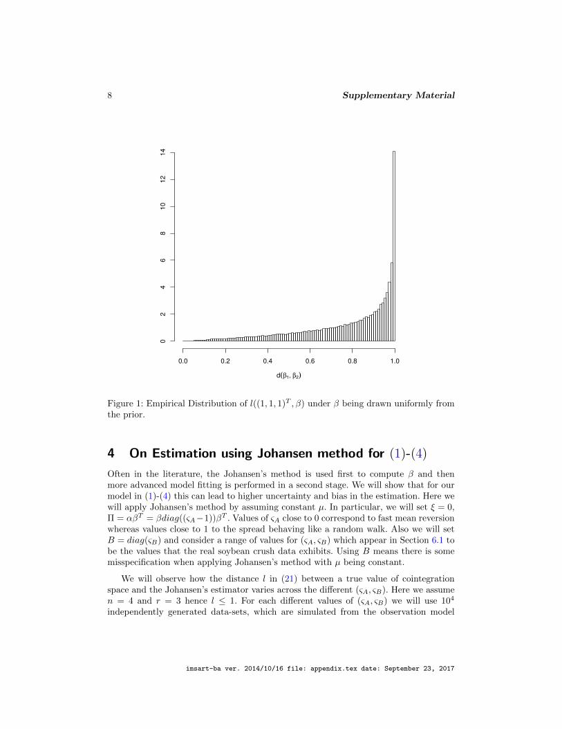
In this simulation, we aim to provide a value of space distances l(β1, β2) which can be

used to determine when sp(β1) and sp(β2) could be considered statistically different

at a 1% significance level. For this purpose, we set β1 = 1√3(1, 1, 1)T and generate 105

uniform realizations of β2 from the prior distribution in (8). We assume β1, β2 ∈ R3×1

in order to be ensure the cointegration rank is 1. For each simulated value of β2, we

compute d(β1, β2). In Figure 1, we present the histogram of these simulated distances

d(β1, β2). It can be found that the 1% quantile of the simulated distribution of d(β1, β2)

under the prior is 0.14. The prior is a uniform distribution on a Stiefel manifold, so we

could use this value to be the threshold for determining whether sp(β1) 6= sp(β2).



d(β1, β2)

0.0 0.2 0.4 0.6 0.8 1.0

02

46

81

01

21

4

Figure 1: Empirical Distribution of l((1, 1, 1)T , β) under β being drawn uniformly fromthe prior.

4 On Estimation using Johansen method for (1)-(4)

Often in the literature, the Johansen’s method is used first to compute β and thenmore advanced model fitting is performed in a second stage. We will show that for ourmodel in (1)-(4) this can lead to higher uncertainty and bias in the estimation. Here wewill apply Johansen’s method by assuming constant µ. In particular, we will set ξ = 0,Π = αβT = βdiag((ςA−1))βT . Values of ςA close to 0 correspond to fast mean reversionwhereas values close to 1 to the spread behaving like a random walk. Also we will setB = diag(ςB) and consider a range of values for (ςA, ςB) which appear in Section 6.1 tobe the values that the real soybean crush data exhibits. Using B means there is somemisspecification when applying Johansen’s method with µ being constant.

We will observe how the distance l in (21) between a true value of cointegrationspace and the Johansen’s estimator varies across the different (ςA, ςB). Here we assumen = 4 and r = 3 hence l ≤ 1. For each different values of (ςA, ςB) we will use 104

independently generated data-sets, which are simulated from the observation model


9

(1), whilst ensuring that the autocorrelation matrix A of zt = βT yt in (5) has spectral

radius smaller than 1. We use 100 uniform random samples of β, for each of which we

generate 100 random realizations of noise process εt. From Figure 2, we see that varying

ςB for a given ςA has a significant impact on the Johansen’s estimator. As expected,

increasing ςB brings about increased level of estimated cointegration space distortion

and wider confidence intervals for l(βJ , βtrue). The same behavior holds when ςA is fixed

and ςB is increasing.

0.6 0.8 0.9 0.95

0.0

0.2

0.4

0.6

0.8

1.0

0.8

0.6 0.8 0.9 0.95

0.0

0.2

0.4

0.6

0.8

1.0

0.85

0.6 0.8 0.9 0.95

0.0

0.2

0.4

0.6

0.8

1.0

0.9

0.6 0.8 0.9 0.95

0.0

0.2

0.4

0.6

0.8

1.0

0.95

Figure 2: Monte Carlo experiment for l(βJ , βtrue). Each panel corresponds to a dif-ferent value of ςA ∈ {0.8, 0.85, 0.9, 0.95}. and we show box-plots for each ςB ∈{0.6, 0.8, 0.9, 0.95}.

5 Synthetic Case Study Figures

In this section, we present the figures for the algorithm validation experiments discussed

in more detail in Section 5 of the main manuscript.



0 50 100 150 200

−4

−2

02

4

0 50 100 150 200

−5

05

0 50 100 150 200

−5

05

0 50 100 150 200

−10

05

10

Figure 3: Estimation of µt(l) for l = 1, . . . , 4: in each panel we show the true µt(l) usedto simulate the data (red line), the posterior mean estimate from the Algorithm 1 (greenline) and 95% posterior confidence intervals (dashed lines).


11

1 1

long_multip[i, j, 10000:1e+05]

Density

−0.7 −0.5 −0.3

02

46

1 2


Density

−0.6 −0.2 0.2

01

23

4

1 3


Density

−0.8 −0.4 0.0

0.0

1.0

2.0

3.0

1 4


Density

0.6 1.0

0.0

1.0

2.0

3.0

2 1


Density

0.0 0.2 0.4

01

23

45

2 2


Density

−1.0 −0.6 −0.2

0.0

1.0

2.0

3.0

2 3


Density

−0.6 −0.2 0.2

0.0

0.5

1.0

1.5

2.0

2 4


Density

−0.2 0.2 0.6

0.0

1.0

2.0

3 1


Density

−0.2 0.0 0.2 0.4

01

23

45

3 2


Density

−0.2 0.2 0.6

0.0

1.0

2.0

3.0

3 3


Density

−1.0 −0.5 0.0

0.0

0.5

1.0

1.5

2.0

3 4


Density

−0.6 −0.2 0.2 0.6

0.0

1.0

2.0

4 1

Density

−0.2 0.2 0.6

0.0

1.0

2.0

3.0

4 2

Density

−0.5 0.0 0.5 1.0

0.0

0.5

1.0

1.5

2.0

4 3

Density

−0.5 0.0 0.5 1.0

0.0

0.5

1.0

1.5

4 4

Density

−1.5 −0.5 0.0

0.0

0.4

0.8

1.2

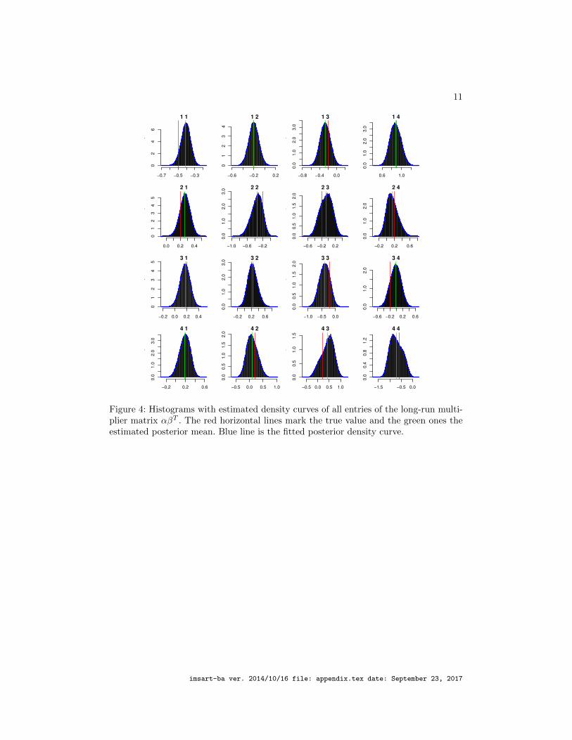
Figure 4: Histograms with estimated density curves of all entries of the long-run multi-plier matrix αβT . The red horizontal lines mark the true value and the green ones theestimated posterior mean. Blue line is the fitted posterior density curve.



1 3 5 7 9 11

−3

−1

01

23

41

●●

●●

●●

●●

●

●●

●

●

●

●●

●

●●●

●

●

●

●

1 3 5 7 9 11

−2

02

4

2

●●

●●

●

●

●●

●

●

●

● ●

●

●

●

●

● ●●

●● ●●

1 3 5 7 9 11

−4

−2

02

4

3

●●

●●

●●

●●

●●

●●

●●

●●

●●

●

●

●●●●

1 3 5 7 9 11

−4

−2

02

44

●●

●●

●●

●

●

●

●

●●

●●

●

●

●●

●

●

●●

●●

Figure 5: Boxplots for posterior of ξ: the green dot indicates the true value and the redone the posterior mean.

ReferencesGupta, A. K. and Nagar, D. K. (1999). Matrix variate distributions, volume 104. CRC

Press. 2

Jain, J., Li, H., Cauley, S., Koh, C.-K., and Balakrishnan, V. (2007). “Numericallystable algorithms for inversion of block tridiagonal and banded matrices.” 7

Rauch, H. E., Striebel, C., and Tung, F. (1965). “Maximum likelihood estimates oflinear dynamic systems.” AIAA journal , 3(8): 1445–1450. 5


supplementary material to 'bayesian inference for …nkantas/sup_material_soybean.pdf ·...

Documents