1

2

3

4

5

6

7

8

9

10

11

Supplementary Material for 12

13

Evaluation of the effect of chickenpox vaccination on shingles epidemiology 14

using agent-based modeling. 15

16

17

18

19

20

21

22

23

24

25

26

27

28

29

30

31

Table of contents 32

1. Supplementary Figure 1: Equations to calculate the shingles immunity waning timer. 33

2. Supplementary Figure 2: An example of the space dependence represented in a distance-based network. 34

3. Supplementary Table 1: Data extracted from sources for the calibration and fitting of the model. 35

4. Supplementary Figure 3: Age-specific proportion of the population with varicella antibody. 36

5. Supplementary Figure 4: Chickenpox and shingles incidence between urban and rural communities, both 37

before and after vaccination. 38

6. Supplementary Figure 5: Simulated and empirical age-specific shingles incidence rate for scenarios that 39

met calibration with various duration of boosting and waning of immunity rates at time 0. 40

7. Supplementary Figure 6: Simulated and empirical age-specific shingles incidence rate for scenarios that 41

did not met calibration with various duration of boosting and waning of immunity rates at time 0. 42

8. Supplementary Figure 7: Simulated and empirical age-specific chickenpox incidence for different 43

duration of boosting and waning of immunity, all scenarios that met calibration at time 0. 44

9. Supplementary Figure 8: Number of shingles cases by age at time 10, 25, 50 and 7 by experiment. 45

10. Supplementary Figure 9: Age distribution of shingles cases in baseline scenario. 46

11. Supplementary Figure 10: Frequency of connections between urban and rural agents. 47

48

49

50

51

52

53

54

55

56

Shingles Immunity Waning Timer = (1) Years Protected Through Infection + (2) Years Protected Through 57

Boosting 58

59

(1) Years Protected Through Infection = min (0,log(forceOfReactivation/InitialCMI)min(0,log(1−waningOfImmunityRateShingles)

60

(2) Years Protected Through Boosting= Number of times an agent comes into significant contact with VZV (in 61

the form of chickenpox or shingles) X The duration in years of each boosting event 62

63

Where: 64

ForceOfReactivation= The strength of shingles reactivation, i.e. the amount of VZV-CMI need to stop 65

reactivation in the form of shingles, the value for each individual in our population is drawn from a gamma 66

distribution. 67

InitialCMI= The initial level of VZV-CMI protection conferred following chickenpox, the value for each 68

individual in our population is drawn from a normal distribution. 69

WaningOfImmunityRateShingles= the rate of annual loss of VZV protection (1/years). The 70

WaningOfImmunityRateShingles is a fixed rate that can be altered in our model using the waning of immunity 71

coefficient. 72

Duration of each boosting event= The number of years of protection gained through each significant boosting 73

event, this value is based on calibration results. 74

75

This equation was derived from the model presented in Ogunjimi et al.25 76

77

Supplementary Figure 1: Equations to calculate the shingles immunity waning timer. 78

79

80

81

82

Consider the two networks shown in the above figure Agents are divided into two age groups, A and B. The 83 table below shows the count of contacts between each of the age groups. This table applies to both networks, 84 even though their arrangement is different. In Figure S2 (A), an infection in age group A in the first quadrant 85 can potentially spread to two other people. In Figure S2 (B), an infection of the same person can potentially 86 spread to the entire population. This demonstrates spatial dependence that is captured by an ABM but not 87 evident when summarizing the network structure in the form of a contact matrix. 88

Age Group A B A 0 8 B 8 8

89

Supplementary Figure 2: An example of the space dependence represented in a distance-based network.90 . 91

92

Supplementary Table 1: Data and references used in the calibration and fitting of the model. 93

Model data calibrated Source outcomes that we compared to model data (by age group)

Years of data collection

Source

Age-specific shingles rates of infection (Parameters varied: Duration of boosting, waning of immunity coefficient, exogenous infection rate, and shingles connection range)

Fig 3 “Age-specific medically attended shingles rates, per 1000 population, and availability of chickenpox vaccine: 1994-98 (pre-licensure)”

- Medically attended (ages: <1, 1-4, 5-9, 10-19, 20-24, 25-29, 30-34, 35-39, 40-44, 45-49, 50-54, 55-59, 60-64, 65-69, 70-74, 75-79, 80-84, 85-89, 90+)

1994-1998 Russell et al. (2014)4

Age-specific chickenpox rates of infection (parameters varied: exogenous infection rate, shingles connection range, underreporting factor)

Table 2 “Mean annual rates of varicella-related outcomes during pre-vaccine (FY1992-1998)”

- Office visits (ages: <1, 1-4, 5-9, 10-19, 20-49 and 50+)

1992-1998 Kwong et al. (2008)27

94

95

96

97

98

99

100

101

102

103

104

105

106

107

108

109

110

111

Supplementary Figure 3: Age-specific proportion of the population with varicella antibody. 112

113

114

115

116

117

118

119

120

121

122

123

124

125

(A) 126

127

128

129

130

131

132

133

134

135

136

137

138

139

140

(B) 141

142

143

144

145

146

147

148

149

150

151

152

153

154

155

156

157

(C) 158

159

160

161

162

163

164

165

166

167

168

169

170

171

172

173

(D) 174

175

176

177

Supplementary Figure 4: Outcomes by urban and rural communities. (A) Chickenpox incidence pre-178 vaccination. (B) Shingles incidence pre-vaccination. (C) Chickenpox incidence post-vaccination. (D) Shingles 179 incidence post-vaccination. 180

(A)

(B)

(C)

(D)

(E)

(F)

Supplementary Figure 5: Simulated and empirical age-specific shingles incidence rate for scenarios that met

calibration with various duration of boostings and waning of immunity rates at time 0. (A) DoB= 2 years, WoI= 0.5.

(B) DoB= 3 years, WoI= 0.55. (C) DoB= 4 years, WoI= 0.6. (D) DoB= 5 years, WoI= 0.63. (E) DoB= 6 years, WoI=

0.68. (F) DoB= 7 years, WoI= 0.74. Blue polygons represent the min and max of the 30 simulated runs.

(A)

(B)

(C)

(D)

Supplementary Figure 6: Simulated and empirical age-specific shingles incidence rate for scenarios that did not

met calibration with various duration of boostings and waning of immunity rates at time 0. (A) DoB= 0.42 years,

WoI= 0.45. (B) DoB= 8 years, WoI= 0.79. (C) DoB= 9 years, WoI= 0.85. (D) DoB= 10 years, WoI= 0.93. Blue

polygons represent the min and max of the 30 simulated runs.

(A)

(B)

(C)

(D)

(E)

(F)

(G)

(H)

(I)

(J)

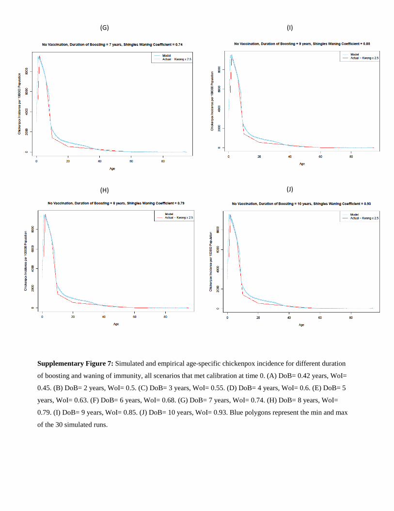
Supplementary Figure 7: Simulated and empirical age-specific chickenpox incidence for different duration

of boosting and waning of immunity, all scenarios that met calibration at time 0. (A) DoB= 0.42 years, WoI=

0.45. (B) DoB= 2 years, WoI= 0.5. (C) DoB= 3 years, WoI= 0.55. (D) DoB= 4 years, WoI= 0.6. (E) DoB= 5

years, WoI= 0.63. (F) DoB= 6 years, WoI= 0.68. (G) DoB= 7 years, WoI= 0.74. (H) DoB= 8 years, WoI=

0.79. (I) DoB= 9 years, WoI= 0.85. (J) DoB= 10 years, WoI= 0.93. Blue polygons represent the min and max

of the 30 simulated runs.

(A)

(B)

(C)

(D)

(E)

(F)

Supplementary Figure 8: Number of shingles cases by age at time 10, 25, 50 and 75 years by scenario. (A) DoB= 2

years, WoI= 0.5. (B) DoB= 3 years, WoI= 0.55. (C) DoB= 4 years, WoI= 0.6. (D) DoB= 5 years, WoI= 0.63. (E)

DoB= 6 years, WoI= 0.68. (F) DoB= 7 years, WoI= 0.74.

Supplementary Figure 9: Age distribution of shingles cases in baseline scenario.

0

500

1000

1500

2000

2500

3000

3500

1 6 11 16 21 26 31 36 41 46 51 56 61 66 71 76 81 86 91 96

Num

ber o

f shi

ngle

s cas

es

Age

Supplementary Figure 10: Frequency of connections between urban and rural agents. Y-axis shows a number of urban agents with one or more connections (x-axis) to rural agents in the model. Total population is 483,526.