Supplementary Information

Nanomodel visualization of fluid injections in tight formations

Junjie Zhong1, Ali Abedini2, Lining Xu1, Yi Xu1, Zhenbang Qi1, Farshid Mostowfi3, David Sinton1

1 Department of Mechanical and Industrial Engineering, University of Toronto, Toronto, ON M5S 3G8, Canada

2 Interface Fluidics Limited, Edmonton, AB T6G 1V6, Canada

3 Schlumberger-Doll Research, One Hampshire Street, Cambridge, Cambridge, Massachusetts 02139, USA

Contents

Section 1: Fabrication and characterization of the nanomodel

Section 2: Experimental setup and procedures

Section 3: Capillarity calculation and Lenormand phase diagram quantification

Section 4: Quantification of the miscible film displacement length and diffusion length in shale reservoirs

Section 5: N2 flooding at 12 MPa

Section 6: CO2 diffusion in the nanomodel during the huff-and-puff injection

Electronic Supplementary Material (ESI) for Nanoscale.This journal is © The Royal Society of Chemistry 2018

Section 1: Fabrication and characterization of the nanomodel

Figure S1. Nanomodel fabrication procedures. (a) Schematic of the nanomodel design. (b) (c)

nanoporous media fabrication, where nanopores (75 nm wide and 50 nm deep) are fabricated

through E-beam lithography and RIE ethching. (d) DRIE etching of the reservoir (200 µm wide and

deep) and thermocouple microchannels (400 µm wide and deep). (e) Inlet/outlet holes drilled for

reservoir microchannels. (f) Anodic bonding of the chip after using Piranha solution (H2SO4:H2O2

= 3:1) cleaning the photoresist.

The nanomodel was fabricated on silicon wafer (chip design is shown in Figure S1a).

To fabricate the nanoporous media on the wafer, E-beam lithography (Vistec EBPG

5000+ Electron Beam Lithography System) was firstly used to generate the

nanoporous pattern on the ZEP-520A resist. After that, the pattern was etched by

RIE (Oxford PlasmaPro 100 Cobra ICP-RIE) to be 50 nm deep, as shown in Figure

S1b and c. On each chip, there were 10 identical nanoporous media distributed

along the microchannel reservoirs. After the nanoporous media was fabricated, the

chip was cleaned in a Piranha solution (H2SO4:H2O2 = 3:1) for 20 min. AZ9260

photoresist was then spin-coated on the wafer to fabricate deep microchannels

and thermocouple channels. We used deep reactive ion etching (DRIE, Oxford

Instruments PlasmaPro Estrelas100 DRIE System) to etch the channels to the

targeting depths (Figure S1d). Afterwards, inlet and outlet holes were drilled on the

silicon substrate of the microchannels, as shown in Figure S1e. The silicon wafer

and a piece of 2.2 mm thick borosilicate glass were then cleaned in the Piranha

solution (H2SO4:H2O2 = 3:1) for another 20 min, and bonded together through

anodic bonding (AML AWB-04 Aligner Wafer Bonder) to seal channels, as shown in

Figure S1g. Bonding chips was at 673.15 K and vacuum with a voltage of 600 V for

10 min (total charge reaching ~1000 mC). Lastly, the chip was cut into the designed

shape with a dicing machine (Disco DAD3220 Automatic Dicing Saw).

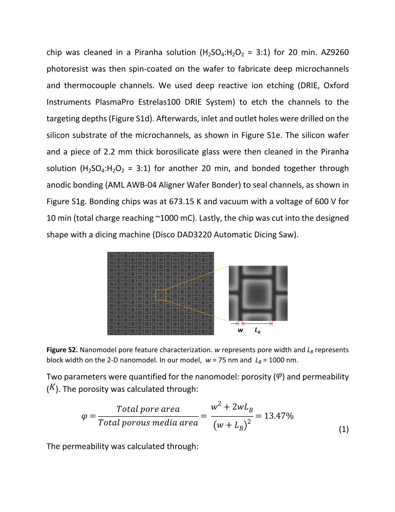
Figure S2. Nanomodel pore feature characterization. w represents pore width and LB represents block width on the 2-D nanomodel. In our model, w = 75 nm and LB = 1000 nm.

Two parameters were quantified for the nanomodel: porosity ( ) and permeability 𝜑( ). The porosity was calculated through:𝐾

(1)𝜑 =

𝑇𝑜𝑡𝑎𝑙 𝑝𝑜𝑟𝑒 𝑎𝑟𝑒𝑎𝑇𝑜𝑡𝑎𝑙 𝑝𝑜𝑟𝑜𝑢𝑠 𝑚𝑒𝑑𝑖𝑎 𝑎𝑟𝑒𝑎

= 𝑤2 + 2𝑤𝐿𝐵

(𝑤 + 𝐿𝐵)2= 13.47%

The permeability was calculated through:

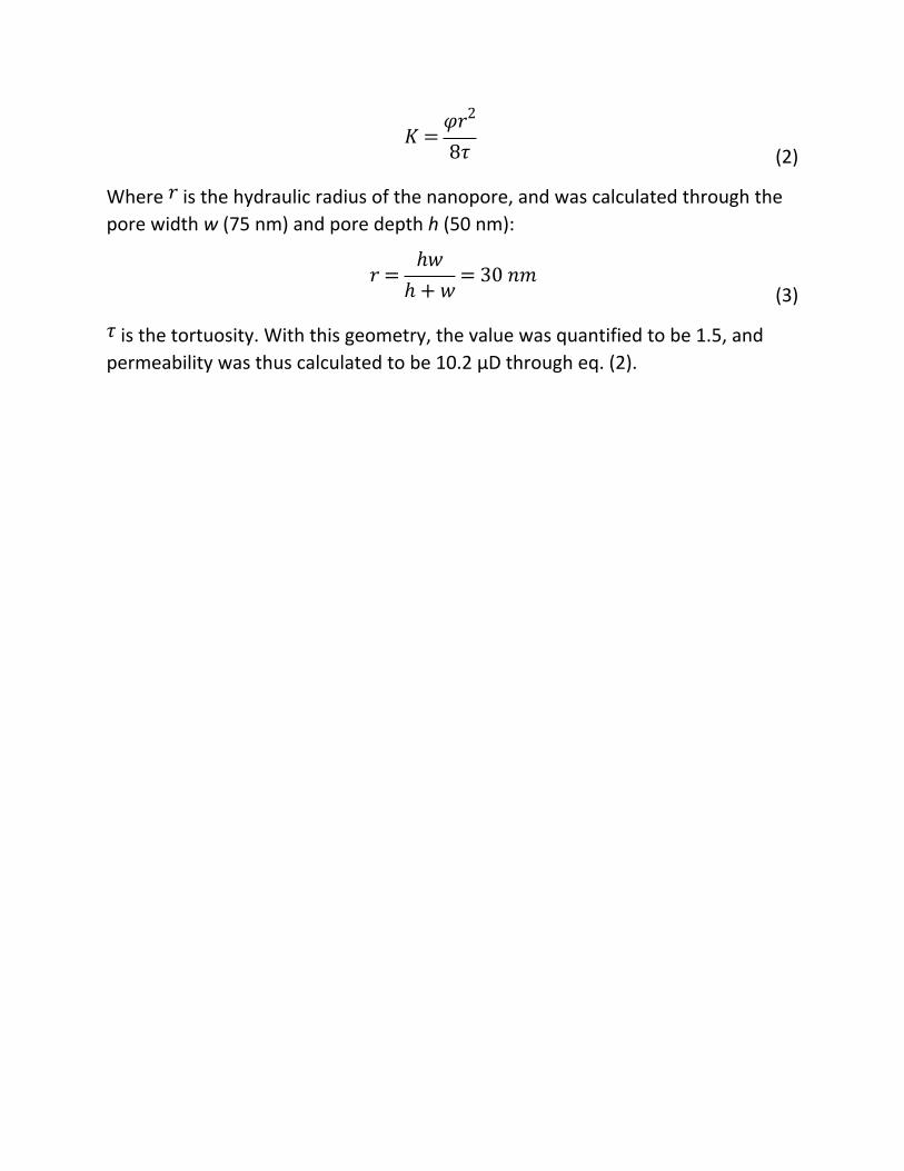
(2)𝐾 =

𝜑𝑟2

8𝜏

Where is the hydraulic radius of the nanopore, and was calculated through the 𝑟pore width w (75 nm) and pore depth h (50 nm):

(3)𝑟 =

ℎ𝑤ℎ + 𝑤

= 30 𝑛𝑚

is the tortuosity. With this geometry, the value was quantified to be 1.5, and 𝜏permeability was thus calculated to be 10.2 µD through eq. (2).

Section 2: Experimental setup and procedures

Figure S3. Diagram of the experimental setup for N2 and CO2 flooding tests. The nanofluidic chip

was mounted on a manifold to connect microchannels with pipes. Pressures of gas as well as oil

were closely controlled through ISCO syringe pump, and monitored through pressure

transducers. Temperature on the chip was introduced through a copper heater controlled by a

water bath (323.15 K), and monitored by thermocouples inserted into the chip close to the

nanoporous media.

Figure S4. Diagram of the experimental setup for CO2 huff-and-puff tests.

To perform the flooding tests, the system (Figure S3) was firstly vacuumed at 2 x

10-7 MPa (PFPE RV8) for 3 hrs at room temperature (293.15 K) to ensure oil filling

fully into the nanoporous media (i.e., no air trapping in the nanoporous media).

After that, the oil was injected into one microchannel through syringe pump

(TELEDYNE ISCO MODEL 260D, resolution at 0.001 MPa), as well as the nanoporous

media at 1 MPa. Due to the capillary force, the filling would stop at the entrance of

the nanoporous media on the gas channel side. Then gas at targeting pressure was

injected into another microchannel. During the gas injection, oil was kept at the

same pressure with gas to avoid any unexpected flooding below the targeting gas

pressure. To start the flooding test, oil pressure was reduced to 5 MPa (taking less

than 3 s). Flooding phenomena were observed directly through an optical

microscope (Leica DM 2700M) and camera connected (Leica DMC 2900).

To perform the huff-and-puff tests (Figure S4), after vacuuming and oil injection,

the oil microchannel was purged by air at 0.8 MPa for 1 hr to clean any residual oil,

ensured by the vanishing of any fluorescence signals in the microchannel. The

system was then vacuumed for another 1 hr to ensure no air trapped in the system.

Afterwards, the gas was injected into both microchannels at targeting pressures,

followed by sealing for 1 hr to allow sufficient gas diffusion into nanoporous media.

In the end, the gas pressure was reduced to targeting value (1 MPa) to produce oil

from the nanoporous media.

Section 3: Capillarity calculation and Lenormand phase diagram quantification

The capillary pressures between the gas phase and oil were calculated using the Young–Laplace equation, which has been validated at nanoscale in previous works1-2:

(4)𝑃𝐶𝑎 = 𝛾 (𝑐𝑜𝑠𝜃ℎ

ℎ/2+

𝑐𝑜𝑠𝜃𝑤

𝑤/2 )Where is the capillary pressure between the gas and oil phase, is the interfacial 𝑃𝐶𝑎 𝛾

tension, is the channel height, 50 nm, is the channel width, 75 nm, and ℎ 𝑤 𝜃ℎ 𝜃𝑤

are the contact angle at channel height and width dimensions (close to zero).

Table 1 shows calculated for all cases discussed in the main text:𝑃𝐶𝑎

Table 1 Capillary pressure calculation for different tests. The values of interfacial tensions are calculated from previous literatures3-4.

Gas species Gas pressure (MPa)

Oil pressure

(MPa)

Pressure drop

(MPa)

Interfacial tension

(mN/m)

Capillary pressure

(MPa)N2 (flooding) 5 5 0 21.7 1.45N2 (flooding) 5.5 5 0.5 21.5 1.43N2 (flooding) 6 5 1 21.3 1.42N2 (flooding) 6.5 5 1.5 21.1 1.41N2 (flooding) 7 5 2 21 1.40N2 (flooding) 9 5 4 20.2 1.35N2 (flooding) 11 5 6 19.5 1.30

CO2 (huff-and-puff) 5 4.05 0.95 14.2 0.95CO2 (huff-and-puff) 7 6.29 0.71 10.7 0.71CO2 (huff-and-puff) 1 -0.42 1.42 21.3 1.42

To quantify the fingering effect during N2 flooding, two parameters (mobility ratio, and capillary number, ) were calculated:𝑀 𝐶𝑎

(5)𝑀 =

𝐾𝑜𝑖𝑙/𝜇𝑜𝑖𝑙

𝐾𝑔𝑎𝑠/𝜇𝑔𝑎𝑠

(6)𝐶𝑎 =

𝜇𝑔𝑎𝑠𝑣

𝛾

Where and are the permeability of gas and oil in the nanomodel (same in 𝐾𝑔𝑎𝑠 𝐾𝑜𝑖𝑙

our case), and are the dynamic viscosity of gas and oil, is the 𝜇𝑔𝑎𝑠 𝜇𝑜𝑖𝑙 𝑣characteristic velocity (displacing rate in our case), and is the interfacial tension. 𝛾

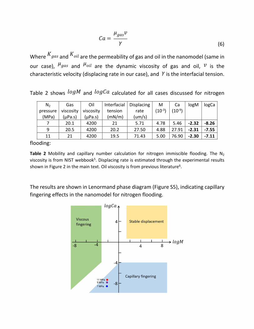
Table 2 shows and calculated for all cases discussed for nitrogen 𝑙𝑜𝑔𝑀 𝑙𝑜𝑔𝐶𝑎

flooding:

Table 2 Mobility and capillary number calculation for nitrogen immiscible flooding. The N2 viscosity is from NIST webbook5. Displacing rate is estimated through the experimental results shown in Figure 2 in the main text. Oil viscosity is from previous literature6.

The results are shown in Lenormand phase diagram (Figure S5), indicating capillary fingering effects in the nanomodel for nitrogen flooding.

N2 pressure (MPa)

Gas viscosity (μPa.s)

Oil viscosity (μPa.s)

Interfacial tension (mN/m)

Displacing rate

(um/s)

M(10-3)

Ca (10-9)

logM logCa

7 20.1 4200 21 5.71 4.78 5.46 -2.32 -8.269 20.5 4200 20.2 27.50 4.88 27.91 -2.31 -7.55

11 21 4200 19.5 71.43 5.00 76.90 -2.30 -7.11

Figure S5. Lenormand phase diagram shows nitrogen flooding in the nanomodel brings capillary

fingering effect, as observed in our experiments.

Section 4: Quantification of the miscible film displacement length and diffusion length in shale reservoirs

Figure S6. Schematic of film-wise displacement in the reservoir.

To simply calculate the speed of film-wise displacement ( ), we considered a 1-D 𝑣

transport diagram as shown in Figure S6. is thus can be expressed as:𝑣

(7)𝑣 =

𝑑𝐿𝑔𝑎𝑠

𝑑𝑡= (𝑃𝑔𝑎𝑠 ‒ 𝑃𝑜𝑖𝑙)𝜑𝑟2 8𝜏[(𝜇𝑔𝑎𝑠 ‒ 𝜇𝑜𝑖𝑙)𝐿𝑔𝑎𝑠 + 𝜇𝑜𝑖𝑙𝐿𝑅]

Where is the length of gas phase traveling in the reservoir, is the gas 𝐿𝑔𝑎𝑠 𝑃𝑔𝑎𝑠

injection pressure, is the reservoir oil pressure, is the porosity of the 𝑃𝑜𝑖𝑙 𝜑

reservoir, is the mean pore radii, is the reservoir tortuosity, is the gas 𝑟 𝜏 𝜇𝑔𝑎𝑠

viscosity, is the oil viscosity, is the total reservoir length (or the reservoir 𝜇𝑜𝑖𝑙 𝐿𝑅

length between the injection and production wells). By integrating eq. (7) with

initial condition ( when t = 0), and considering the condition 𝐿𝑔𝑎𝑠 = 0 𝜇𝑜𝑖𝑙 ≫ 𝜇𝑔𝑎𝑠

(more than 100 times), one gets the expression for as a function of recovery 𝐿𝑔𝑎𝑠

time ( ):𝑡

(8)𝐿𝑔𝑎𝑠 = 𝐿𝑅 ‒ 𝐿𝑅

2 ‒𝜑𝑟2(𝑃𝑔𝑎𝑠 ‒ 𝑃𝑜𝑖𝑙)

4𝜇𝑜𝑖𝑙𝜏𝑡

The diffusion length ( ) follows Fick’s law, and can be expressed as a function 𝐿𝐷𝑖𝑓𝑓

of recovery time ( ):𝑡

(9)𝐿𝐷𝑖𝑓𝑓 = 2

𝐷𝜏

𝑡

Where the gas diffusivity into oil is , as the diameter of gas molecules (e.g., CO2, 𝐷

~0.3 nm) are still much smaller than the pore size (e.g., 60 nm in our case). We

assume bulk diffusivity (~ )7 can still be applied here. The tortuosity 5 × 10 ‒ 9 𝑚2/𝑠

( ) will also affect the effective diffusivity in a periodic porous system8.𝜏

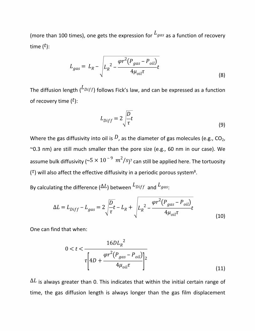
By calculating the difference ( ) between and :∆𝐿 𝐿𝐷𝑖𝑓𝑓 𝐿𝑔𝑎𝑠

(10)∆𝐿 = 𝐿𝐷𝑖𝑓𝑓 ‒ 𝐿𝑔𝑎𝑠 = 2

𝐷𝜏

𝑡 ‒ 𝐿𝑅 + 𝐿𝑅2 ‒

𝜑𝑟2(𝑃𝑔𝑎𝑠 ‒ 𝑃𝑜𝑖𝑙)4𝜇𝑜𝑖𝑙𝜏

𝑡

One can find that when:

(11)

0 < 𝑡 <16𝐷𝐿𝑅

2

𝜏[4𝐷 +𝜑𝑟2(𝑃𝑔𝑎𝑠 ‒ 𝑃𝑜𝑖𝑙)

4𝜇𝑜𝑖𝑙𝜏 ]2

is always greater than 0. This indicates that within the initial certain range of ∆𝐿

time, the gas diffusion length is always longer than the gas film displacement

length. For the nanomodel in this work, , , , 𝐿𝑅 = 10 ‒ 3 𝑚 𝜑 = 0.13 𝑟 = 30 𝑛𝑚

and , the time range is thus calculated to be 𝜏 = 1.5 𝑃𝑔𝑎𝑠 ‒ 𝑃𝑜𝑖𝑙 = 6 𝑀𝑃𝑎

. From the experiments, we noticed that the gas breakout happens 0 < 𝑡 < 23 𝑠

first as fingers, while film displacement captures the fingers at ~20 s (Figure 3 (A)).

The order of magnitude match here indicates that the calculation can describe the

gas breakout phenomena well. For a real shale reservoir, parameters are available

from orders of magnitude, where is on the order of , is on the order of 𝐿𝑅 10 𝑚 𝜑

0.1, is on the order of 100 nm, is on the order of 1 and is on the order 𝑟 𝜏 𝑃𝑔𝑎𝑠 ‒ 𝑃𝑜𝑖𝑙

of 10 MPa. The range is thus calculated to be (~4 months). Therefore, 0 < 𝑡 < 107 𝑠

within the first few months for the miscible flooding in a low pressure reservoir,

gas breakout could happen first, while the miscible flooding will follow the initial

production.

It is noting that, the analytic model here separates the pressure driven fluid viscous

transport and the free molecular diffusion effect for a simplification of calculation

and comparison. These two effects are inherently coupled and can be potentially

solved with computational fluidic methods. The model also simplifies the flow

boundary conditions, to strictly follow the non-slip boundary condition from

classical fluid mechanics for both gas and liquid phases, as the pore scale here is at

60 nm, and the pore surface is smooth (roughness at ~0.2 nm). At a smaller sub-10

nm pore scale, the fluid slip boundary condition might be important to be

considered, especially for the gas phase. The slip boundary condition will in general

lead to a reduced viscous transport resistance in nanopores. However, these

simplifications are not expected to affect the order of magnitude estimations, as

well as the qualitative conclusions demonstrated here.

Section 5: N2 flooding at 12 MPa

Figure S7. High pressure nitrogen flooding (12 MPa nitrogen and 10 MPa oil) result. The FOR is

~31 %.

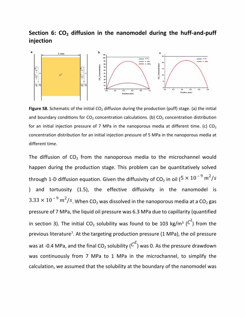
Section 6: CO2 diffusion in the nanomodel during the huff-and-puff injection

Figure S8. Schematic of the initial CO2 diffusion during the production (puff) stage. (a) the initial

and boundary conditions for CO2 concentration calculations. (b) CO2 concentration distribution

for an initial injection pressure of 7 MPa in the nanoporous media at different time. (c) CO2

concentration distribution for an initial injection pressure of 5 MPa in the nanoporous media at

different time.

The diffusion of CO2 from the nanoporous media to the microchannel would

happen during the production stage. This problem can be quantitatively solved

through 1-D diffusion equation. Given the diffusivity of CO2 in oil ( 5 × 10 ‒ 9 𝑚2/𝑠

) and tortuosity (1.5), the effective diffusivity in the nanomodel is

. When CO2 was dissolved in the nanoporous media at a CO2 gas 3.33 × 10 ‒ 9 𝑚2/𝑠

pressure of 7 MPa, the liquid oil pressure was 6.3 MPa due to capillarity (quantified

in section 3). The initial CO2 solubility was found to be 103 kg/m3 ( ) from the 𝐶𝐼

previous literature7. At the targeting production pressure (1 MPa), the oil pressure

was at -0.4 MPa, and the final CO2 solubility ( ) was 0. As the pressure drawdown 𝐶𝐸

was continuously from 7 MPa to 1 MPa in the microchannel, to simplify the

calculation, we assumed that the solubility at the boundary of the nanomodel was

linearly changing (i.e., , where is total time for the pressure

𝑑𝐶𝑑𝑡

=‒ (𝐶𝐼 ‒ 𝐶𝐸)

𝑡 𝑡

depletion). Based on these conditions, the CO2 concentration distributions at

different time are shown in Figure S7(b). At 20 s, the average CO2 concentration (

) in the nanoporous media was ~63 kg/m3. While at 200 s, the 𝐶𝐴 =

𝐿

∫0

𝐶(𝑥)𝑑𝑥

𝐿

average CO2 concentration was only ~13 kg/m3. Similarly, for an initial gas injection

pressure at 5 MPa, the oil pressure was at 4 MPa due to capillarity (section 3), the

CO2 solubility is 25 kg/m3. At 20 s, the CO2 concentration distribution is shown in

Figure S8, where the average value was ~15 kg/m3.

Oil displacement in the nanomodel initiated from 7 MPa (Fig. 4A), while at 5 MPa,

during depressurization there was no oil displacement. The reason is the significant

change of CO2 solubility at different injection pressures because of capillarity in

nanoconfinement. Here, when injected CO2 was at 5 MPa, the oil pressure was

actually 4 MPa due to capillarity (section 3). Under this condition, the CO2

concentration in the oil is expected to be 25 kg/m3 as determined elsewhere7.

Similarly, with CO2 at 7 MPa, the oil pressure was 6.3 MPa (section 3), and CO2

concentration reaches 103 kg/m3. After a 20 s production, the CO2 pressure was

reduced to 1 MPa. The oil was under tension at -0.4 MPa (capillary pressure ~1.4

MPa, section 3), and CO2 solubility in oil approaches zero. This leads to (i) CO2

accumulating and generating bubbles within the nanoporous media, pushing oil

out, and/or (ii) CO2 diffusing out from the nanoporous media. The former requires

supersaturated CO2 accumulating and overcoming capillary pressure to form gas

bubbles (1 MPa), with a minimum CO2 density at 17 kg/m3. A 5 MPa CO2 injection

pressure leads to low average remaining CO2 concentration in oil after a 20 s

production (~15 kg/m3). Bubbles was thus not likely to form. While for the initial

CO2 injection pressure at 7 MPa, the average remaining CO2 concentration is at 63

kg/m3 greater than 17 kg/m3 (section 6). Bubbles were observed to grow during the

production stage to displace oil (Fig. 4A). The total production time would also

affect the oil recovery. For example, at the same 7 MPa CO2 injection pressure but

for a 200 s production (compared to 20 s), no trapped oil was observed to be

produced from the nanomodel. The reason is due to the gas diffusion eliminating

most CO2 in the nanoporous media (average remaining CO2 concentration is only

13 kg/m3). Likewise, bubbles were unable to generate and displace oil.

Reference

1. Zhong, J.; Riordon, J.; Zandavi, S. H.; Xu, Y.; Persad, A. H.; Mostowfi, F.; Sinton, D., Capillary Condensation in 8-nm Deep Channels. J. Phys. Chem. Lett. 2018, 9, 497-503.2. Zhong, J.; Zandavi, S. H.; Li, H.; Bao, B.; Persad, A. H.; Mostowfi, F.; Sinton, D., Condensation in One-Dimensional Dead-End Nanochannels. ACS Nano 2017, 11, 304-313.3. Hemmati-Sarapardeh, A.; Ayatollahi, S.; Ghazanfari, M.-H.; Masihi, M., Experimental determination of interfacial tension and miscibility of the CO2–crude oil system; temperature, pressure, and composition effects. J. Chem. Eng. Data. 2013, 59, 61-69.4. Hemmati-Sarapardeh, A.; Ayatollahi, S.; Zolghadr, A.; Ghazanfari, M.-H.; Masihi, M., Experimental determination of equilibrium interfacial tension for nitrogen-crude oil during the gas injection process: the role of temperature, pressure, and composition. J. Chem. Eng. Data. 2014, 59, 3461-3469.5. P.J. Linstrom and W.G. Mallard, E., NIST Chemistry WebBook, NIST Standard Reference Database Number 69. National Institute of Standards and Technology, Gaithersburg MD, 20899, http://webbook.nist.gov, 2016.6. Lansangan, R.; Smith, J., Viscosity, density, and composition measurements of CO2/West Texas oil systems. SPE Reservoir Eng. 1993, 8, 175-182.7. Sharbatian, A.; Abedini, A.; Qi, Z.; Sinton, D., Full characterization of CO2–oil properties on-chip: solubility, diffusivity, extraction pressure, miscibility, and contact angle. Anal. Chem. 2018, 90, 2461-2467.8. Berezhkovskii, A. M.; Zitserman, V. Y.; Shvartsman, S. Y., Effective diffusivity in periodic porous materials. J. Chem. Phys. 2003, 119, 6991-6993.