SUPPLEMENTARY INFORMATIONDOI: 10.1038/NGEO1797

NATURE GEOSCIENCE | www.nature.com/naturegeoscience 1

1

Supplementary Information

Continental-scale temperature variability during the last two millennia PAGES 2k Consortium

Moinuddin Ahmed, Kevin J. Anchukaitis, Asfawossen Asrat, Hemant P. Borgaonkar, Martina Braida, Brendan M. Buckley, Ulf Büntgen, Brian M. Chase, Duncan A. Christie, Edward R. Cook, Mark A. J. Curran, Henry F. Diaz, Jan Esper, Ze-Xin Fan, Narayan P. Gaire, Quansheng Ge, Joëlle Gergis, J. Fidel González-Rouco, Hugues Goosse, Stefan W. Grab, Rochelle Graham, Nicholas Graham, Martin Grosjean, Sami T. Hanhijärvi, Darrell S. Kaufman, Thorsten Kiefer, Katsuhiko Kimura, Atte A. Korhola, Paul J. Krusic, Antonio Lara, Anne-Marie Lézine, Fredrik C. Ljungqvist, Andrew M. Lorrey, Jürg Luterbacher, Valérie Masson-Delmotte, Danny McCarroll, Joseph R. McConnell, Nicholas P. McKay, Mariano S. Morales, Andrew D. Moy, Robert Mulvaney, Ignacio A. Mundo, Takeshi Nakatsuka, David J. Nash, Raphael Neukom, Sharon E. Nicholson, Hans Oerter, Jonathan G. Palmer, Steven J. Phipps, Maria R. Prieto, Andres Rivera, Masaki Sano, Mirko Severi, Timothy M. Shanahan, Xuemei Shao, Feng Shi, Michael Sigl, Jason E. Smerdon, Olga N. Solomina, Eric J. Steig, Barbara Stenni, Meloth Thamban, Valerie Trouet, Chris S.M. Turney, Mohammed Umer, Tas van Ommen, Dirk Verschuren, Andre E. Viau, Ricardo Villalba, Bo M. Vinther, Lucien von Gunten, Sebastian Wagner, Eugene R. Wahl, Heinz Wanner, Johannes P. Werner, James W.C. White, Koh Yasue, Eduardo Zorita — Correspondence to: Darrell.Kaufman@nau.edu Part I: Notes, figures and tables

Note A – PAGES 2k Network data archival and management Note B – Alternative reconstructions Note C – Analysis of forcings Fig. S1. Temperature in PAGES 2k regions compared with global temperature Fig. S2. Proxy temperature reconstructions for the seven regions, original resolution Fig. S3. Alternative temperature reconstructions compared with original reconstructions Fig. S4. 30-year mean standardized temperatures, alternative & original reconstructions Fig. S5. Area-weighted average temperature, alternative & original reconstructions Fig. S6. Regression analysis of individual site-level proxy records by region Table S1. Correlations between instrumental targets and alternative reconstructions Table S2. Regression statistics for long-term trends Table S3. 20th century temperatures compared with the preceding 500 years Table S4. Simulated regional temperture trends related to individual forcings

Part II: Explanation of each continental-scale temperature reconstruction 1. Arctic 2. Europe 3. Asia 4. North America 5. South America 6. Australasia 7. Antarctica 8. Africa Figs. S7 to S16 Table S5

References Other supplementary information for this manuscript includes: Database S1 – All proxy records metadata and raw data Database S2 – Regional temperature reconstructions (original & alternative)

2

Part I: Explanation of data management, alternative reconstructions, and supplementary figures and table Note A - PAGES 2k Network data archival and management To facilitate the distribution and assessment of climate data and to encourage contributions by data generators, all derived reconstructions and associated proxy records that form the 2k Network are permanently archived and available through internet-accessible data archives. The primary outlet is the World Data Center for Paleoclimatology, operated by the Paleoclimatology Branch of the National Climatic Data Center, United States National Oceanic and Atmospheric Administration (NOAA-Paleo)1. Additional archive sites are PANGAEA2, and NEOTOMA3, the North American archive of pollen, plant macrofossil, and other microfossil paleoenvironmental data operated by the Illinois State Museum. NOAA follows international conventions for data description and archiving, ensuring the PAGES 2k data are accessible beyond the paleoclimatology community and for future generations. NOAA distributes the PAGES 2k Network data descriptions using OAI-PMH harvesting and providing protocols, making the PAGES 2k data visible beyond the NOAA web site.

At the NOAA-Paleo site, a special set of PAGES 2k webpages has been established, organized by the PAGES 2k continental-scale regional working groups4. Each regional page provides an interactive map showing the location of study sites for proxy records considered relevant to the PAGES 2k project. Primary information can be retrieved by hovering over a study site’s display symbol, and clicking on the symbol to access the related data record. On the same webpage, a listing of these data sets is displayed for each region, in addition to a link to this publication’s webpage where the records that were used for the regional reconstructions and the reconstructions themselves can be accessed. The archive will grow as the community continues to publish relevant research results. When age models and data are revised, the "last update" metadata field and associated notes will be updated accordingly.

Search capabilities for the NOAA-Paleo site have been structured to accommodate PAGES-2k-specific searches, both for the overall 2k Network and for each continental-scale region. The general search feature5,6 uses logic operators to refine searches by allowing the user to specify, e.g., both a PAGES 2k region and a data contributor, or both a PAGES 2k region and a set of proxy/archive types. Additional functionality is planned that will allow users to select a user-defined subset of proxy data for a region, and to generate a single downloadable file of the requested data in NetCDF, ASCII, or Excel™ formats.

3

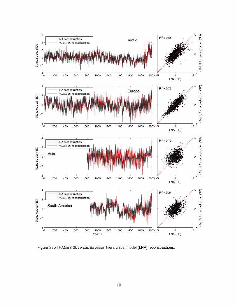
Note B – Alternative reconstructions To assess the extent to which the choice of reconstruction method might influence our primary conclusions, we applied three additional data-analysis procedures to generate alternative reconstructions from each region. These include a (1) pairwise comparison7, which was also used for the Arctic reconstruction, (2) Bayesian hierarchical model8, and (3) basic non-calibrated composite. We used the same proxy data as were used by the PAGES 2k Network regional groups (Database S1). For each region, the reconstruction target was calculated as the mean annual temperature from HadCRUT4 (ref. 9) using the area-weighted values over the domains shown in Figure 1. For Antarctica, the HadCRUT4 data were truncated prior to 1946 because the data become too sparse. The r-values for correlations between the target and reconstructions are in Table S1. The PAGES 2k Network annual-scale reconstructions are compared with these alternative reconstructions in Figure S3. The standardized 30-year averages are compared for the four reconstruction methods in Figure S4. The 30-year area-weighted averages across all regions are compared for the four reconstructions methods in Figure S5. The results of the regression analysis for the long-term trends for all reconstruction methods are listed in Table S2, and the temperature differences between the 20th century and the preceding 500 years for all reconstruction methods are listed in Table S3. The alternative reconstructions were not optimized in the same way as was done for the PAGES 2k Network reconstructions and they are not intended as substitutes for the primary reconstructions. Instead, they are meant to give a sense of the robustness of the overall results. Differences probably reflect the different screening and weighting procedures used in the 2k Network reconstructions compared with the more generalized approach used for the alternative procedures. The PAGES 2k Network reconstructions for three regions (North America tree rings, Australasia and Asia) were derived from spatially explicit reconstructions, which adds considerable complexity, including spatially variable weightings of individual proxy records. The alternate reconstructions do not accommodate this complexity. The pairwise comparison (PaiCo) procedure7 is a nonlinear maximum likelihood method that, for each proxy record, records the pairwise comparisons between each sample value and then finds a time series that best agrees with these comparisons. The method is loosely similar to finding the time series that has the best Kendall’s tau correlation coefficient with all proxy records. Proxy records with values that scale negatively with temperature (as listed in Database S1) were inverted. We set the regularization parameter value to 1 and optimized until the log likelihood changed less than 10-6%. The method automatically uses variance matching to calibrate the result to the instrumental target. Agreement between the PaiCo and the 2k Network regional temperature reconstructions ranges from r2 = 0.16 to 0.84 (average = 0.53; excluding the Arctic 2k Network reconstruction, which itself was based on PaiCo) (Fig. S3). The Bayesian hierarchical model developed by Li, Nychka and Ammann (ref. 8; referred to as “LNA”) is a linear Bayesian method that finds the temperature time series that best correlates with each proxy record. The method is loosely similar to linear regression. For this procedure, each record was individually standardized to zero mean

4

and unit variance over the length of the record. This was done only to improve convergence, since the model for LNA contains shift, scale and noise variance parameters for each record and, therefore, standardization is not required. We fixed the autocorrelation coefficients to 0 to simplify the model and to stabilize the calculations. We drew 1000 samples from the Bayesian posterior distribution and used the latter 500 to calculate the reconstructed temperature as the average of the samples. Agreement between Bayesian hierarchical model and the 2k Network regional temperature reconstructions ranges from r2 = 0.04 to 0.76 (average = 0.32) (Fig. S3). The match for Asia and North America (tree ring-based and pollen-based) are outliers among this set of alternative reconstructions. The PAGES 2k Network reconstructions in these regions do not appear unusual in other aspects, however, such as the temperature differences between the 20th century and the preceding 500 years (Table S3). Basic composites were constructed by standardizing then averaging the individual proxy records from each region. Proxy records with values that scale negatively with temperature (as listed in Database S1) were inverted, then all records were standardized to have zero mean and unit variance relative to the period of common overlap for all records within a region. The Calvo_2002 record in the Arctic was excluded because it precluded any common overlap among the records. Records from sites located in a single 5°x 5° grid were averaged and then re-standardized to unit variance to generate a single series for each grid box. Regional composites were calculated as area-weighted averages of the gridded series. To avoid additional assumptions and for simplicity, no attempt was made to calibrate the basic composites to absolute temperature. The term “composite” rather than “reconstruction” is used because the standard-deviation units are not scaled to regional temperature. Agreement between the 2k Network regional temperature reconstructions and the basic composites ranges from r2 = 0.24 to 0.88 (average = 0.55) (Fig. S3).

5

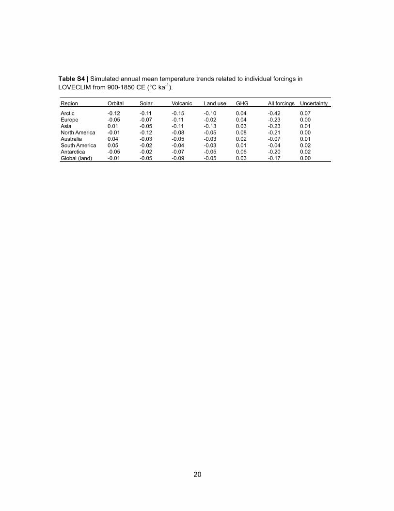
Note C – Regional temperature trends associated with individual forcings simulated by LOVECLIM To estimate the long-term temperature trend associated with individual forcings, an ensemble of simulations was performed with the Earth system model of intermediate complexity, LOVECLIM10 driven by one forcing at a time. LOVECLIM has simpler dynamics and a coarser resolution than current general circulation models (GCMs). Its atmospheric component is ECBilt211, a quasi-geostrophic model with T21 horizontal resolution (corresponding to about 5.6° x 5.6°). CLIO, the ocean component12, is a general circulation model with a horizontal resolution of 3° x 3°. A simple vegetation model (VECODE13) is also activated in the configuration selected here, at the same resolution as in ECBILT. Because of these simplifications, LOVECLIM is much faster than the GCMs, allowing the required large number of long simulations to be performed. The experiment including all forcings was driven by natural (solar, volcanic and orbital) and anthropogenic forcings (greenhouse gases (GHG), various aerosols, land use) following the PMIP3-CMIP5 protocol14 over the period 850-1850 CE. The simulations started from an equilibrium state corresponding to the forcings in 850 CE, and the first 50 years of integration were excluded to reduce the influence of this spin-up procedure. The solar irradiance followed the reconstruction from ref. 15 between 850 and 1609 CE, and from ref. 16 between 1610 and 2000 CE. The Earth's orbital parameters evolved according to the calculations of ref. 17. The forcing due to volcanic activity was derived from ref. 18, and was implemented through anomalies in solar irradiance at the top of the atmosphere. The anthropogenic land-use changes were based on the reconstruction of global agricultural areas and land cover of ref. 19 from 850 to 1700 CE, and on the reconstruction of ref. 20 from 1700 CE onwards. To reduce the influence of internal variability, an ensemble of five simulations was performed for each forcing. Because five simulations comprise a relatively small ensemble, we also analyzed an ensemble of five simulations driven by no forcing to provide an estimate of the uncertainty associated with the internal variability of the modeled system. In the uncertainty limit of our experiments, the response to all forcings is not significantly different from the sum of the response to the individual forcings. The ensemble-mean temperature trends indicate that the four forcings contribute the same order of magnitude to the annual mean cooling trend simulated in each region (Table S4). Because this result is based one climate model only, it should be considered as illustrative. LOVECLIM is known to underestimate the response to forcing in low latitudes. Furthermore, only one estimate was used for each forcing. Results from GCMs using one forcing at a time are required to determine which part of LOVECLIM results are robust. To our knowledge, such simulations are not yet available. We suspect that the sign of the response more robust than the magnitude of the trend.

6

Figure S1 | Comparison between the area-weighted mean annual temperature within the PAGES 2k regional domains as plotted in Figure 1 (land and ocean) and global mean annual temperature. All data are from HadCRUT4 (ref. 9).

7

Figure S2 | Proxy temperature reconstructions for the seven regions of the PAGES 2k Network. Temperature anomalies are relative to the 1961-1990 CE reference period. Grey lines around expected-value estimates indicate uncertainty ranges as defined by each regional group (Supplemental Information Part II), namely: Antarctica, Australasia, North America pollen, and South America = ± 2SE; Asia = ± 2 RMSE; Europe = 95% confidence bands; Arctic = 90% confidence; North American trees = upper/lower 5% bootstrap bounds (these are inherently narrower than those of many other regions because they are reported at decadal and multi-decadal, rather than annual resolution). Instrumental temperatures are area-weighted mean annual temperatures over the reconstruction domains shown in Figure 1 from HadCRUT4 (ref. 9) land and ocean, rather than the target temperature series used in the regional reconstructions. This facilitates a uniform comparison among regions using a data series that extends to 2010. The actual reconstruction targets for each region are specified in Table 1. Reconstruction time series are listed in Supplementary Database S2.

8

Figure S3 | Comparisons between the PAGES 2k Network regional temperature reconstructions (Fig. S2) and three alternative reconstruction procedures using the same proxy data from each region. The three alternative procedures are: a, pairwise comparison7 (PaiCo); b, Bayesian hierarchical model8 (LNA); and c, basic non-calibrated composite (composite). Reconstructions were standardized to have a mean of zero and unit variance. Individual proxy records are listed in Database S1; reconstructions are in Database S2.

9

10

11

12

13

14

Figure S4 | Comparison between a, the PAGES 2k Network regional temperature reconstructions (same as Fig. 2) and three alternative reconstruction procedures using the same proxy data for each region including: b, basic composites, c, Bayesian hierarchical model7, and d, pairwise comparison8. Grids are 30-year averages. All series were standardized relative to the period of common overlap for all regions (1200 to 1965 CE). Data are listed in Database S2.

15

Figure S5 | Standardized 30-year-mean temperatures averaged across all seven continental-scale regions for four reconstruction methods. a, PAGES 2k Network regional temperature reconstructions (same as Fig. 4b), b, basic composites, c, Bayesian hierarchical model, and d, pairwise comparisons. Blue symbols are area-weighted averages using domain areas listed in Table 1, and bars show 25th and 75th unweighted percentiles to illustrate the variability among regions; open black boxes are unweighted medians; red line in (a) is the 30-year-average annual global temperature from the HadCRUT4 (ref. 9) time series relative to 1961-1990.

16

Figure S6 | Least-squares linear regression analysis of individual proxy records from all regions, including those that extend back to 1 CE (left column) and to 1000 CE (right column). Pie diagrams show the proportion of records that have statistically significant (p < 0.05) and non-significant slopes. Histograms show the distribution of slope and p values by region. The dashed red lines in the lower panels represent the 0.05 and 0.95 p-values; p-values for some records are undeterminable (i.e., the autocorrelation -adjusted sample size is < 2 and df < 0).

17

Table S1 | Correlations (r-value) between alternative reconstruction and HadCRUT4 1900-2000 annual temperatures (ref. 9).

a “PAGES 2k” = original reconstruction by PAGES 2k regional network; r-values differ from those in Table 1 because they are based on a different (and uniform) target than those used for each region as reported in Part II of the Supplementary Information; Composite = basic composite (this study); PaiCo = pairwise comparison8; LNA = Bayesian hierarchical model7. b PAGES 2k North America tree-ring-based reconstruction is resolved at decadal scale.

Reconstruction

methoda Arctic Europe AsiaNorth America

South America Australasia Antarctica

PAGES 2k 0.49 0.57 0.43 —b 0.55 0.78 0.17Composite 0.54 0.49 0.50 0.60 0.48 0.77 0.14PaiCo 0.49 0.47 0.38 0.60 0.54 0.70 0.05LNA Algorithm returns the exact instrumental value (i.e., r = 1.00)

18

Table S2 | Summary statistics for least-squares linear regressions for temperature reconstructions from each region.

Full record to 1900 CE 1000-1900 CE Full record to 1850 CE 1000-1850 CE

Region Start date (CE)

Slope (°C

ka-1)p

Slope (°C

ka-1)p

Slope (°C

ka-1)p

Slope (°C

ka-1)p

Original PAGES 2k Network resonstructionsArctic 1 -0.29 <0.001 -0.47 <0.001 -0.31 <0.001 -0.60 <0.001Europe 1 -0.23 <0.001 -0.09 0.13 -0.25 <0.001 -0.16 <0.05Asia 800 -0.23 <0.05 -0.21 <0.05 -0.26 <0.001 -0.26 <0.05N. America - trees 1200 -0.32 <0.10 - - -0.33 <0.10 - -N. America - pollen 480 -0.13 ND -0.34 <0.10 -0.10 ND -0.30 0.12South America 857 -0.13 <0.05 -0.14 <0.05 -0.12 <0.05 -0.12 <0.10Australasia 1000 -0.27 <0.001 -0.27 <0.001 -0.30 <0.001 -0.30 <0.001Antarctica 167 -0.27 <0.001 -0.27 <0.001 -0.26 <0.001 -0.25 <0.001

Pairwise comparions (PaiCo) reconstructionsArctic 1 -0.29 <0.001 -0.47 <0.001 -0.31 <0.001 -0.60 <0.001Europe 1 -0.19 <0.001 -0.19 <0.001 -0.21 <0.001 -0.35 <0.001Asia 800 -0.20 <0.01 0.05 0.26 -0.24 <0.001 -0.11 0.12N. America - trees 1200 -0.13 0.09 - - -0.17 0.06 - -N. America - pollen 480 -0.32 ND -0.01 0.50 -0.35 0.42 -0.04 0.48South America 857 -0.11 0.07 -0.12 0.10 -0.14 <0.05 -0.16 0.06Australasia 1000 0.04 0.72 0.05 0.76 0.02 0.61 0.03 0.64Antarctica 167 -0.21 <0.001 -0.19 <0.01 -0.20 <0.001 -0.18 <0.01

Bayesian hierarchical model reconstructionsArctic 1 -0.31 <0.001 -0.62 <0.001 -0.34 <0.001 -0.79 <0.001Europe 1 -0.13 <0.001 -0.35 <0.001 -0.14 <0.001 -0.45 <0.001Asia 800 -0.13 0.13 0.00 0.50 -0.23 <0.05 -0.13 0.23N. America - trees 1200 -0.01 0.52 - - 0.65 0.99 - -N. America - pollen 480 -0.96 ND 0.48 ND -1.20 ND 0.18 NDSouth America 857 -0.22 <0.001 -0.24 <0.001 -0.24 <0.001 -0.27 <0.01Australasia 1000 -0.03 0.19 -0.03 0.20 -0.16 <0.001 -0.15 <0.001Antarctica 167 -0.68 <0.001 -0.66 <0.01 -0.67 <0.001 -0.64 <0.01

Basic non-calibrated composites. Slopes have units of SD units per 1000 yearsArctic 1 -0.13 <0.01 0.9 <0.001 -0.13 <0.01 -1.10 <0.001Europe 1 -0.22 <0.001 0.03 0.61 -0.24 <0.001 -0.08 0.22Asia 800 -0.19 <0.01 -0.18 <0.01 -0.19 <0.01 -0.18 <0.10N. America - trees 1200 -0.04 0.32 - - -0.06 0.28 - -N. America - pollen 480 -1.80 ND -1.00 ND -1.90 ND -1.20 NDSouth America 857 -0.29 <0.05 -0.31 <0.10 -0.38 <0.05 -0.42 <0.05Australasia 1000 -0.78 <0.001 -0.78 <0.001 -0.55 <0.001 -0.55 <0.001Antarctica 167 -0.44 <0.001 -0.45 <0.001 -0.43 <0.001 -0.44 <0.001

Red font = not signficant at p < 0.05; ND = not determinable (i.e., the autocorrelation-adjusted sample size is < 2 and df < 0)Time series used for all regression analyses are listed in Database S2

19

Table S3 | Temperatures (°C) of the 20th century compared with the preceding five centuries based on three reconstruction methods.

Period (CE) Arctic Europe AsiaNorth America TR Australasia

South America Average South Hem North Hem

PAGES 2k Network1911-2000 -0.13 0.09 -0.04 -0.10 -0.19 -0.15 -0.09 -0.17 -0.041401-1910 -1.02 -0.32 -0.42 -0.33 -0.35 -0.34 -0.46 -0.34 -0.52Difference 0.88 0.42 0.39 0.23 0.16 0.19 0.38 0.18 0.48SE 0.11 0.02 0.14

Bayesian hierarchical model 1911-2000 -0.01 -0.03 -0.13 0.02 -0.16 -0.24 -0.09 -0.20 -0.041401-1910 -1.04 -0.43 -0.69 0.61 -0.53 -0.48 -0.43 -0.51 -0.39Difference 1.03 0.40 0.56 -0.59 0.37 0.24 0.33 0.30 0.35SE 0.22 0.07 0.34

Pairwise comparison1911-2000 -0.13 0.05 -0.01 0.02 -0.25 -0.18 -0.08 -0.21 -0.021401-1910 -1.00 -0.41 -0.43 -0.14 -0.48 -0.41 -0.48 -0.44 -0.50Difference 0.87 0.47 0.42 0.16 0.23 0.24 0.40 0.23 0.48SE 0.11 0.00 0.15

Note: excludes Antarctica

20

Table S4 | Simulated annual mean temperature trends related to individual forcings in LOVECLIM from 900-1850 CE (°C ka-1).

Region Orbital Solar Volcanic Land use GHG All forcings Uncertainty

Arctic -0.12 -0.11 -0.15 -0.10 0.04 -0.42 0.07Europe -0.05 -0.07 -0.11 -0.02 0.04 -0.23 0.00Asia 0.01 -0.05 -0.11 -0.13 0.03 -0.23 0.01North America -0.01 -0.12 -0.08 -0.05 0.08 -0.21 0.00Australia 0.04 -0.03 -0.05 -0.03 0.02 -0.07 0.01South America 0.05 -0.02 -0.04 -0.03 0.01 -0.04 0.02Antarctica -0.05 -0.02 -0.07 -0.05 0.06 -0.20 0.02Global (land) -0.01 -0.05 -0.09 -0.05 0.03 -0.17 0.00

21

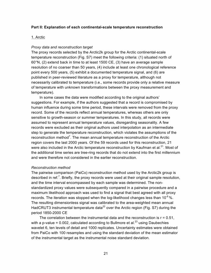
Part II: Explanation of each continental-scale temperature reconstruction 1. Arctic Proxy data and reconstruction target The proxy records selected by the Arctic2k group for the Arctic continental-scale temperature reconstruction (Fig. S7) meet the following criteria: (1) situated north of 60°N, (2) extend back in time to at least 1500 CE, (3) have an average sample resolution of no coarser than 50 years, (4) include at least one chronological reference point every 500 years, (5) exhibit a documented temperature signal, and (6) are published in peer-reviewed literature as a proxy for temperature, although not necessarily calibrated to temperature (i.e., some records provide only a relative measure of temperature with unknown transformations between the proxy measurement and temperature).

In some cases the data were modified according to the original authors’ suggestions. For example, if the authors suggested that a record is compromised by human influence during some time period, these intervals were removed from the proxy record. Some of the records reflect annual temperatures, whereas others are only sensitive to growth-season or summer temperatures. In this study, all records were assumed to represent annual temperature values, disregarding seasonality. A few records were excluded as their original authors used interpolation as an intermediate step to generate the temperature reconstruction, which violates the assumptions of the reconstruction method7. The mean annual temperature reconstruction of the Arctic region covers the last 2000 years. Of the 59 records used for this reconstruction, 21 were also included in the Arctic temperature reconstruction by Kaufman et al.21. Most of the additional time series are tree-ring records that do not extend into the first millennium and were therefore not considered in the earlier reconstruction.

Reconstruction method The pairwise comparison (PaiCo) reconstruction method used by the Arctic2k group is described in ref.7. Briefly, the proxy records were used at their original sample resolution, and the time interval encompassed by each sample was determined. The non-standardized proxy values were subsequently compared in a pairwise procedure and a maximum likelihood approach was used to find a signal that best agreed with all proxy records. The iteration was stopped when the log-likelihood changes less than 10-6 %. The resulting dimensionless signal was calibrated to the area-weighted mean annual HadCRUT3 instrumental temperature data22 over the Arctic region (Fig. S7) during the period 1850-2000 CE

The correlation between the instrumental data and the reconstruction is r = 0.51, with a p-value = 0.002, calculated according to Bullmore et al.23 using Daubechies wavelet 6, ten levels of detail and 1000 replicates. Uncertainty estimates were obtained from PaiCo with 100 resamples and using the standard deviation of the mean estimator of the instrumental target as the instrumental noise standard deviation.

22

2. Europe Proxy data and reconstruction target Calibration target data for the Europe summer (June-August, JJA) temperature reconstruction were derived from CRUTEM4v, comprising mean monthly surface air temperature anomalies (relative to 1961-1990) on a 5°x5° land-only grid spanning the period 1850-2010 CE. Grid cells over the European domain were selected within the range 35°-70°N, 10°W-40°E. Grid cells over Iceland and small North Atlantic islands were excluded, thus yielding a total of 61 retained cells. Missing months in the selected cells were infilled using the regularized expectation maximization (RegEM) algorithm with ridge regression24 to yield a time-continuous monthly anomaly grid. The infilled European data were used to compute the average JJA temperature in each grid cell, from which an area-weighted25 mean summer temperature index was computed for the selected European domain. Differences between computed raw (with gaps) and infilled mean summer temperature indices are small and occur primarily prior to 1900 CE when the amount of missing data, particularly in the Mediterranean region, is most pronounced.

Eleven annually resolved tree-ring and documentary records from ten European countries/regions were used for the reconstruction (Database S1; Fig. S8). Records were selected based upon their seasonal temperature signals (ranging from May-June, June-July and April-September) as described in the original papers, a minimum record length (>700 years), and sample replication throughout time. In regions where multiple high-resolution records are available (northern Scandinavia), reconstructions based on maximum latewood density (MXD) measurements were preferred. All tree-ring data were detrended using the regional curve standardization (RCS) method to retain low-frequency variance in the resulting mean chronologies26. The northern Scandinavian series retains millennial-scale variance related to long-term changes in orbital forcing27, a frequency range that is likely restricted in the other dendroclimatic records. The Torneträsk data are based on Briffa et al.28 ending in 1980 CE, and have been extended to 2004 through mean and variance matching over 1951-1980 CE using MXD data derived from x-ray fluorescence measurements29. The central European summer temperature reconstruction is based on documentary data30. It is the only time series that was calibrated against instrumental data, covers a large area in Europe, and extends back only 500 years.

Reconstruction method The nested composite-plus-scale” (CPS32,33) reconstruction was computed using nine nests reflecting the availability of predictors back in time. A CPS reconstruction was computed for each nest by standardizing (normalizing and centering) the available predictor series over the calibration interval, and subsequently calculating a weighted composite in which the relative weight of each proxy was determined by the strength of the correlation with the European mean summer temperature index. Finally, each composite was centered and scaled to have the same variance as the target index

23

during the calibration interval. The CPS methodology was implemented using a resampling scheme for validation and calibration33 that uses 104 years for calibration and 50 years for validation (the last year of uniformly available predictor series is 2003 CE, providing 154 years of overlap with the target index). The initial calibration period extended from 1850-1953 CE and was incremented by one year until reaching the final period of 1900-2003 CE, yielding a total of 51 reconstructions for each nest. Within each calibration step, the 50 years excluded from calibration were used for validation. For each nest, the final CPS reconstruction was computed as the median reconstructed value in each year within the 51-member reconstruction ensemble. Uncertainties were estimated from the mean standard deviation of the residuals across all of the validation intervals; twice this standard deviation estimate was added to the maximum and minimum ensemble values in each year to derive the 95% confidence intervals of the median reconstruction. The final nested reconstruction was combined by splicing the median reconstruction and estimated uncertainties of each nest such that every reconstructed year was derived from the nest with the maximum possible predictors. Cross correlations between each of the derived nests during their period of overlap reflect strong coherence among the estimates and lend further support to the robustness of the reconstruction estimates of the individual nests.

Validation statistics across all reconstruction ensemble members within each nest indicate skillful CPS summer temperature reconstructions. The mean reduction of error (RE) and coefficient of efficiency (CE) statistics34 across the 51 validation intervals in each nest are positive (RE: 0.424-0.642; CE: 0.257-0.538). Benchmarking experiments using 1000 realizations of first-order autoregressive (AR1) red noise time series as predictors and autocorrelations approximating those of the available proxy records were also performed. These experiments yielded maximum mean RE and CE benchmark values below the mean values achieved for the actual reconstruction across all nests. The mean correlation coefficients across all nests were all higher than the 95% significance level r = 0.25 assuming a one-tailed probability distribution (r = 0.74-0.86). Similar to the RE and CE results, the mean correlation coefficient across all validation intervals was higher in each reconstruction nest than the maximum mean correlation achieved in the red noise benchmarking experiments.

24

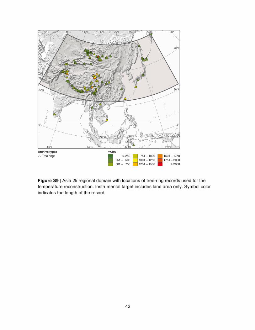
3. Asia Proxy data and reconstruction target The instrumental temperature field used for reconstruction is based on global CRU TSv3.1, 0.5° gridded monthly temperature data (1901-2009)35, which was degraded to 2°, resulting in a total of 773 grid points to reconstruct. Figure S9 shows the temperature domain with the 229-chronology tree-ring network used as the basis for the reconstruction. The available chronologies are sparse and distributed irregularly, which limits the quality of the temperature reconstruction, although this tree-ring network is denser than that used to successfully reconstruct drought over monsoon Asia36.

The calibration period (1951-1989 CE) was chosen following Cook et al.36 to incorporate the period of best quality instrumental data beginning in 1951, and it ends in the year when almost all available tree-ring data can be used for reconstruction. The validation period (1920-1950 CE) choice is a compromise between using the best quality pre-1951 data for validation and providing enough years of data for reasonably robust validation testing. We reconstructed past summer (June-July-August) temperatures, corresponding to the photosynthetically active warm season.

Reconstruction method We used the point-by-point regression (PPR) method presented by Cook et al.37 to reconstruct summer temperature from tree rings. PPR sequentially reconstructs individual grid points of climate over a field using principal components regression (PCR).

As originally formulated for reconstructing drought (PDSI) over North America37, PPR required two user-defined input parameters that were optimized for reconstructing the gridded climate field: a search radius and a screening probability. However, the basic PPR methodology was modified for reconstructing PDSI by Dai et al.38 over monsoon Asia because the density of the tree-ring chronology network and quality of the PDSI data used were both markedly inferior to those products used over North America. This made the previously determined search radius and screening probability impractical to use. Thus, the following changes were made to PPR:

1) An ensemble-based approach for reducing the noise level in the reconstructions was

developed in which the fixed screening probability was replaced by the variable weighting of the candidate tree-ring chronologies found with a given search radius. The weighting (wgt) applied to the tree-ring chronologies was related to some power p of the correlation r of each tree-ring chronology with the grid point PDSI being reconstructed, i.e. wgt = rp. This is expressed as wTR = uTR*rp, where wTR is the weighted tree-ring series and uTR is the original unweighted tree-ring series in standard normal deviate form. Varying the power over a range from 0 to 2 allowed for a series of weightings to be applied to the same suite of tree-ring chronologies found with a given search radius, thus perturbing the covariance matrix of predictors used in PCR. A total of eight powers were applied (0, 0.10, 0.25, 0.50, 0.67, 1.0, 1.5, and 2.0), thus creating an ensemble of eight reconstructed temperature fields, which were

25

then averaged to produce an ensemble mean field and the regional summer temperature anomaly index reconstruction presented here.

2) An optimal search radius of 1500 km was objectively determined by directly estimating the e-folding correlation decay distance over the domain by correlating all pairwise grid points of summer temperature and plotting those correlations against the distance between the grid point pairs being correlated. Having made these determinations on how to reconstruct summer temperatures over Asia using PPR, three more data-based decisions were made that directly affect our results:

3) Only tree ring series that began on or before 1600 CE were used as candidates for reconstruction based on the 1500 km search radius and the r>0 screening criterion described above. Doing so eliminated the shorter tree-ring chronologies that tend to be more deficient in low-frequency variance due to the “segment length curse”39.

4) The chronologies found within each grid point 1500 km search radius and retained as predictors in weighted PCR had to be positively correlated with summer temperature (r>0) over the calibration period, with rp naturally down-weighting the more weakly correlated series used as predictors in PCR depending on the choice of p, with no down-weighting applied for the limiting case of p = 0. The reason for requiring r > 0 is our belief that the directly correlated effects of temperature on tree growth (e.g. direct temperature effects on physiological processes and photosynthetic rates) are likely to produce a more reliable expression of past temperature variability compared to inversely correlated temperatures effects on growth which are more often related to moisture stress (that is, an inverse temperature effect due to evapotranspiration demand). Consequently, some of the 229 tree-ring chronologies never passed the r>0 threshold and, therefore, were not used for reconstruction. This was the only predictor variable screening applied to the tree-ring predictors used in the PCR phase of PPR, and it was completely restricted to the 1951-1989 calibration period. In no case was the 1920-1950 validation period temperature data used for any kind of data screening.

5) To minimize the impact of high autocorrelation or trend on the determination of which tree rings correlated positively (r > 0) with temperature over the calibration period, this simple sign-based screening test was applied after first-order autocorrelation (“red noise”) was removed from the calibration period tree-ring and temperature data by fitted first-order autoregressive (AR1) models. In addition, three correlation tests were applied to the determination of r > 0: the parametric Pearson product-moment correlation, the non-parametric Spearman rank correlation, and a robust form of the Pearson correlation based on the bi-square weight function40. Only if all three correlations were positive was a tree-ring variable retained for input into PCR and the rp weighting applied to each chronology was based on its average r of those three estimates. However, once the tree rings were selected in this way for r>0 based on the first-order autoregressive (AR1) “pre-whitened“ data, the actual reconstructions were produced using the original tree-ring chronologies and temperature data with all of their original persistence or trend intact. This procedure was applied on both t and t+1 tree-ring predictors following the use of lagged tree-ring variables as predictors described in Cook et al.36.

26

The reconstructed summer temperature anomaly (Fig. S2) is the average of all relevant grid-point reconstructions after being expressed as anomalies from the 1961-1990 mean, and covers the period 800-1989 CE. The uncertainty is expressed as ± 2 RMSE of the reconstruction over the calibration period.

The calibration and validation statistics indicate a modest level of calibration skill (r2

= 0.393, RE = 0.327), with some validation skill also indicated (r2 = 0.144, p < 0.05, 1-tailed), but validation RE and CE were both negative. The cause of this latter problem appears to be due largely to the way in which the tree-ring estimates fell progressively below the actual data from 1950 to 1901 CE. It is difficult to say if the lack of low-frequency matching between actual and reconstructed values is due solely to the tree-ring estimates or related to insufficient instrumental data in the pre-1951 period. The latter cannot be readily dismissed in our opinion. For this reason, we believe that this reconstruction is worth further evaluation as a tentative first-order estimate of summer temperatures over monsoon Asia north of 23°N since 800 CE. However, substantial uncertainties remain, particularly at low frequencies, and skill is low over substantial portions of the domain, requiring continued evaluation and refinement.

27

4a. North America — High-frequency tree-ring reconstruction Proxy data and reconstruction target Two semi-independent tree-ring data sets (approximately 30% overlap) were used in the reconstruction. The first data set extends temporally from 1500-1980 CE, covering an area in western mid-latitude North America bounded by 30°-55°N, 95°-130°W, with one additional chronology in west-central Mexico (Fig. S10). This data set was used to make a spatially-explicit annual temperature reconstruction over the above target domain from 1500-1980 CE41. The second data set extends temporally from 1200-1987 CE, and includes sites in eastern North America in the same mid-latitude range and a few sites in the western Arctic region (Fig. S10). This data set was used for the first time in the PAGES 2k project to make a spatially explicit annual temperature reconstruction over the above target domain from 1200-1987 CE. The data are generally ring-width chronologies, with a few density measurements included; the data are available from the International Tree Ring Data Base (ITRDB)42.

The first proxy data set was spatially calibrated and validated against the HadCRUT3v 5°x5° gridded surface temperature data for the selected region. Calibration was done over 1904-1980 and validation over 1875-1903, the periods during which data coverage was available for the full region (calibration) and at least 30% of the regional grid cells had data coverage (validation)41. The second proxy data set was spatially calibrated and validated against an infilled version of the same instrumental data set43, and thus was able to be calibrated and validated over longer periods (1886-1987 for calibration and 1850-1885 CE for validation).

The infilled version of the instrumental data set was also used for the eastward extension (to 75°W) of reconstructed decadal average temperatures, as explained in the following section.

Reconstruction methods Two spatially-explicit reconstructions were developed for the temperate western region of North America 30°-55°N, 95°-130°W, at 5°x5° spatial resolution, based on the two data sets described above, the first covering 1500-1980 and the second covering 1200-1987. A spatially-explicit reconstruction farther east was not successfully validated. The reconstructions employed a truncated EOF (TEOF) method discussed in the literature as principal components spatial regression (PCSR)34, abbreviated PCSR-TEOF. Details of the reconstruction, methodology, and associated simulation tests are described in the SOM of Wahl and Smerdon41. The 1500-1980 reconstruction is identical to that reported in Wahl and Smerdon41, and is referred to as WS12. The 1200-1987 reconstruction is new to the PAGES 2k effort. WS12 exhibits validation grid-scale RE/spatial-mean RE/spatial-mean CE of 0.40/0.62/0.42, respectively, while the 1200-1987 reconstruction exhibits 0.13/0.53/0.31 for the same measures, respectively. The analysis of North American tree rings was designed to generate a spatial field reconstruction of temperature, a key goal of the PAGES 2k project. The regional mean time series was then extracted from the gridded temperature reconstruction. The additional rigor needed for spatially-explicit statistical skill resulted in a cutoff of 1200 CE,

28

as determined by the North American PAGES 2k team in conjunction with regional dendroclimatologists who developed the new proxy data set used in the 1200-1987 reconstruction. The description below focuses on the regional mean annual temperature value derived from the spatial field reconstructions. Future studies will focus on developing a longer regional mean temperature reconstruction based on longer tree-ring records and other proxy records from North America.

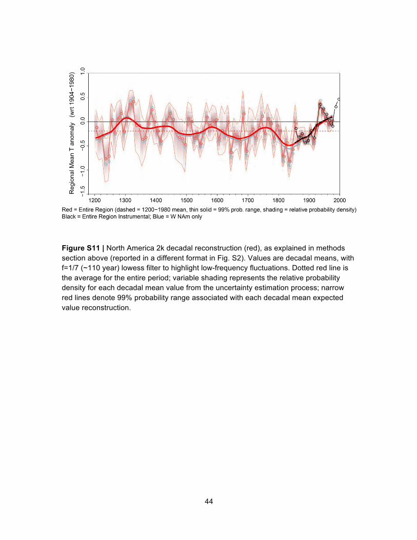
Because the 1200-1987 reconstruction, while well-validated, exhibits lower skill than the WS12 reconstruction, WS12 was used as the reconstruction for 1500-1980 CE and was joined with the 1200-1987 reconstruction to cover the period 1200-1499 CE. To ensure comparability across the splice at 1499/1500 CE, WS12 was regressed onto the 1200-1987 reconstruction over 1500-1980 CE, and then this regression and the 1200-1987 reconstructed values were used to fit WS12-consistent values for the regional spatial mean during 1200-1499 CE. On the basis of instrumental data at the decadal scale, the domain spatial average for temperate western North America exhibits generally good spatial correlation in the same latitude band eastward to 75°W. Thus, the combined western reconstruction was decadally-averaged across its domain and used as the predictor in a calibration against the instrumental domain decadal average for the larger region 30-55°N, 75-130°W, for a period covering 1850-1980 (Fig. S11). Finally, this calibration fit (r2 = 0.93) was used to reconstruct decadal averages of annual temperature over the larger domain for the entire 1200–1979 period (n = 78). In both regressions, the fitted values were scaled so that their variance matched that of the target data during the fitting period.

Uncertainty was estimated using the uncertainty ensembles generated for both the WS12 and the 1200-1987 reconstructions (cf. Wahl and Smerdon41 for the statistical bootstrap method used) in a two-step Monte Carlo design. In this design, the process described above to estimate the EV reconstruction was repeated for each possible combination of five hundred WS12 with five hundred 1200-1987 ensemble members. The 90% probability range estimated by this analysis is shown in Figure S2. Note that these probability ranges are for the decadal means and thus are significantly narrower than the corresponding ranges for annual values would be expected to be, from the theory of the standard error of the mean.

Additional information In temperate western North America, many of the tree-ring chronologies are expected to be more sensitive to moisture than to temperature, at least at the site-level scale. The PCSR-TEOF procedure used for the high-frequency spatial reconstructions (Wahl and Smerdon41) approaches the reconstruction process at a different spatial scale; it evaluates the temporal relationships between the time-varying weights (PCs) of EOF patterns of temperature and the time-varying weights (PCs) of EOF patterns of the dendroclimatological data. Screening of the proxy data happens at this level; specifically, the retained proxy PCs are required to have a level of correlation, established empirically, with one or more of the leading 50% EOF-PCs of the instrumental data, evaluated over the calibration period. In conjunction with this screening, an additional evaluation process determines the number of proxy and instrumental EOF-PCs to retain

29

in the final reconstruction (Wahl and Smerdon41, SOM). Using the proxy information in such an EOF-based manner enables extraction of temperature-related information that is contained within the overall spatial proxy EOF structure and its time-varying weights, including information that may arise due to covariation of moisture and temperature patterns. It has the additional potential advantage that truncation of the EOFs used in the reconstruction can reduce noise in both the proxy and instrumental data sets. This assumes that the instrumental EOF patterns and their pattern-specific (i.e., time invariant) singular value weights stay reasonably stable over time. This assumption was examined by Wahl and Smerdon41, and found to be reasonable in the experimental context of the evaluation.

Paleoclimatologically, the key idea is that the time weights of the spatial patterns of the proxy data can potentially exhibit linear relationships with the time weights of the spatial patterns of the instrumental data in ways that allow successful calibration and validation at both the spatially-explicit and aerially-averaged levels. This is the case for the WS12 and 1200-1987 spatial reconstructions. The individual reconstruction validation statistics reported above show this (cf. also paragraph immediately below), and graphical comparison against the target instrumental data in both calibration and validation indicates this as well (Wahl and Smerdon41). Perhaps the strongest indication of the potential for skill of this method is the comparison of the blue (W NAM decadal average temperature reconstruction) and black (instrumental decadal average temperature for the region east to 75°W) time series in Figure S11. The larger-region red time series (reported in another form and centered to the period 1961-1990 in Fig. S2) is the result of the calibration of the larger-region instrumental data (black) on the western-region reconstruction (blue), as described above, which follows the decadal instrumental target quite closely (r2 = 0.93).

Wahl and Smerdon’s41 examination of reconstruction efficacy comparing real-proxy data with noise-only proxy data also acts as a controlled experiment in this context. The control is the ensemble of reconstructions created using the noise-only proxies, which have the same AR structure as the original proxy PCs, but are otherwise random data, and the treatment is the ensemble of reconstructions created using the real-proxy PCs. In such a control/treatment set-up, the goal is to evaluate whether the treatment group has statistically distinguishable effects on the outcomes relative to the control group; in this case the outcomes concern various measures of reconstruction skill. Wahl and Smerdon41 demonstrate that this is robustly the case for the real proxy-based reconstructions using the PCSR-TEOF method, which clearly and unequivocally separate from those derived using the noise-only data and demonstrate clear skill (Wahl and Smerdon41). Perhaps most strongly, the histogram for the PCSR-TEOF real-proxy regional mean reconstruction ensemble during validation (Wahl and Smerdon41) centers almost spot-on to the actual instrumental value, which is the expected outcome when real climatological information is encoded in the proxy data and the reconstruction process introduces little amplitude loss or gain.

30

4b. North America — Low-frequency pollen reconstruction A principal component analysis (PCA) was performed using four North American regional pollen-based temperature reconstructions44 specifically those based on pollen sequences from deciduous, hardwood, boreal, and mountain ecoregions of North America (Fig. S10). The prairie ecoregion reconstruction for the center of Northern America was not used as its vegetation is mainly controlled by precipitation. Mean annual temperature reconstructions were used instead of summer temperature anomalies as in Viau et al.44 for a more direct comparison to the tree-ring based mean annual temperature reconstruction (hereafter named D1200 for decadal-1200). Furthermore, the regional mean annual temperature reconstructions were resampled at 30-year intervals. The resulting PCA scores (360-1950 CE; n = 54) were then included in a stepwise multiple linear regression against D1200. For this purpose, D1200 was smoothed using a ~110 year lowess filter and sampled every 30 years to approximately match the time scale and sampling resolution of the pollen-based reconstructions. Three combined PC axes explaining 87% of the common variance in the pollen reconstructions were retained in the stepwise regression and explained 33.4% of the variance in D1200.

Uncertainty was estimated based on the 1 and 2 standard error (SE) limits for the pollen-based reconstructions and the SE of the regression model. SE uncertainty bands for the pollen-based reconstructions were only available from 480 CE onwards due to the resampling at 30-year intervals (for comparison to D1200) and the temperature reconstruction was thus truncated at this date. The SEs for the pollen-based reconstructions were developed using a Monte Carlo resampling technique that generated random sequences by sampling values at each time step of the individual pollen series within its uncertainty limits. This process was repeated 10,000 times to generate the pollen-based reconstruction uncertainty bands. These were then inputted into the previously developed PCA and multiple linear regression equations to determine the component of the overall 1SE and 2SE uncertainty limits that is inherent in the pollen-based reconstruction method. The pollen-based reconstruction 1SE and 2SE limits estimated in this manner were augmented at each time step with regression error. Regression error was estimated as 1SE and 2SE limits of the regression model of D1200 for an individual pollen time series. Further uncertainty due to the fact that the predictands y (D1200) are probabilistic estimates of the true population of y-values, was estimated by the 1SE and 2SE of the smoothed D1200 time series. For this purpose, a ~110 year lowess filter was applied to each of the 250,000 ensemble members of the D1200 reconstruction (see uncertainty calculations in high-frequency tree-ring reconstruction section). Estimated standard deviations were then calculated across the ensemble members for each decade, and averaged over the entire reconstruction period (1200-1980). Finally, the squares of the three (assumed independent) errors were added and the square root of this sum was taken as an estimation of total error.

31

5. South America Proxy data and reconstruction target The regional temperature reconstruction for the South America region is an update of Neukom et al.45, with a slightly modified proxy network that includes 23 sites (Fig. S12). Specifically: (i) Remote proxies from outside South America were removed to obtain full independence from the other continental reconstructions. This affected three records from the Australasian domain. (ii) New records that became available since the analysis of Neukom et al.45 were included. Neukom & Gergis46 provide an overview of the full available proxy network. The new records are: Cascayunga Cave, Peru47; Le Quesne precipitation reconstruction48; Lago Plomo49; CAN tree-ring composites 2, 6, 9 and 3150, CAN composites 3251; CAN composites 33-34, Heim Morena Este and Torre Morena 4 (previously unpublished). The new records were screened by correlating them with the reconstruction target (southern South American spatial mean) and including only records with significant correlations (p < 0.05). Correlations were calculated over the 1901-1995 CE calibration period. Significance levels were adjusted for AR(1) autocorrelation. Four tree-ring records from the central Andes passed this screening procedure (CAN composites 2, 6, 9 and 31).

For a reconstruction target, we used the spatial mean of the CRU TSv3.0 land-surface temperature grid over the southern South American domain 20°S-65°S and 30°W-80°W over the period 1901-1995 CE45.

Reconstruction methods Two different reconstruction techniques were applied: principal component regression45,52,53 (PCR), and composite plus scaling45 (CPS). We used an ensemble-based reconstruction method52,53. For both methods (PCR and CPS), an ensemble of 3000 members was generated by creating varying reconstruction settings for each realization by randomly applying the following operations: - Removing two predictors from the full predictor matrix. - Selecting a calibration period of 60-80 (non-successive) years between 1901-1995

CE and using the remaining 15-35 years for verification. - Varying the percentage of total variance of the predictor matrix explained by the

retained PCs between 50% and 90% by varying the number of PCs used. This randomization was not applied in CPS as no PCs are calculated in this approach.

- Scaling the weight of each proxy record in the PC analysis with a factor of 0.67 to 1.5. This randomization was not applied in CPS as no PCs are calculated in this approach. The mean of the combined PCR/CPS 6000-member ensemble was considered our

“best estimate” temperature reconstruction. The reconstruction confidence interval was defined as the combined calibration and ensemble standard error (SE), calculated as !" = !!"#! + !!"#! with σres denoting the standard deviation of the regression residuals and σens the standard deviation of the ensemble members. For further details on the reconstruction methods we refer to Gergis et al.52 (for the ensemble approach) and

32

Neukom et al.45 (for general descriptions of PCR and CPS). Temperatures were reconstructed back to 857 CE before which only three proxy records are available. Reconstruction skills were assessed by computing the RE and r2 values. REs were calculated for each proxy nest over the period 1901-1995 by averaging the values of all ensemble members that were used for calibration and verification, respectively. For both PCR and CPS the RE values were positive over the whole reconstruction period (PCR: RE calibration: 0.11-0.71, verification: 0.04-0.62; CPS: RE calibration: 0.10-0.67, verification: 0.01-0.59) and the PCR (CPS) r2 were 0.25-0.72 (0.28-0.69) for the calibration, and 0.21-0.62 (0.24-0.61) for the verification period.

33

6. Australasia Proxy data and reconstruction target Australasia is herein defined as the land and ocean areas of the Indo-Pacific and Southern Oceans bounded by 110°E-180°E, 0°-50°S. Our instrumental target was calculated as the September-February (SONDJF) spatial mean of the HadCRUT3v 5°x5° monthly combined land and ocean temperature grid9,54 for the Australasian domain over the 1900-2009 period.

Our temperature proxy network (Fig. S13) was drawn from a broader Australasian domain: 90°E-140°W, 10°N-80°S (details provided in Neukom and Gergis46). This proxy network showed optimal response to Australasian temperatures over the SONDJF period, and contains the austral tree-ring growing season during the spring-summer months.

The proxy data were correlated against the grid cells of the target (HadCRUT3v SONDJF average). To account for proxies with different seasonal definitions than our target SONDJF season (for example calendar year averages) we calculate the correlations after lagging the proxies for -1, 0 and 1 years. Records with significant (p < 0.05) correlations with at least one grid-cell within a search radius of 500 km from the proxy site were included in the reconstruction. All data were linearly detrended over the 1921-1990 period and AR(1) autocorrelation was taken into account for the calculation of the degrees of freedom55. For coral record with multiple proxies (Sr/Ca and δ18O) with significant correlations, only the proxy record with the higher absolute correlation was selected to ensure independence of the proxy records. Missing values in the predictor matrix during the calibration period (0.4%) were infilled using principal component regression45,56.

We performed an ensemble ordinary least squares regression principal component reconstruction (PCR) analysis53,57 using the 1921-1990 period for calibration and verification. Further description of the PCR method is provided by Luterbacher et al.58, and details of the extension of the ensemble approach are described below. To assess reconstruction uncertainty associated with proxy selection and calibration, a 3000-member ensemble of reconstructions was calculated creating a varying reconstruction setting for each realization by randomly: - Removing five predictors from the full predictor matrix. In the early part of the

reconstruction (1000-1456 CE) where five or fewer proxies are available, the number of predictors used for each ensemble member varies between one and five.

- Varying the percentage of total variance of the predictor matrix explained by the retained PCs between 60% and 90% by varying the number of PCs used.

- Selecting a calibration period of 35-50 (non successive) years between 1921-1990 and using the remaining 20-35 years for verification.

- Scaling the weight of each proxy record in the PC analysis with a factor of 0.67 to 1.5.

To avoid variance biases due to the decreasing number of predictors back in time, the reconstructions of each model were scaled to the variance of the instrumental target over the 1921-1990 period. The mean of the 3000-member ensemble was considered

34

our “best estimate” temperature reconstruction. To assess low frequency changes in Australasian temperatures, the ensemble mean was smoothed using a 30-year loess filter, which effectively removes variations with periods shorter than 15 years.

The ensemble PCR method allows us to quantify not only the traditional regression residual-based uncertainties referred to as “calibration error”59, but also the spread of the ensemble members generated from the random selection of the reconstruction parameters, described as the “ensemble error”. The reconstruction confidence interval was defined as the combined calibration and ensemble standard error (SE), calculated as !" = !!"#! + !!"#! with σres denoting the standard deviation of the regression residuals and σens the standard deviation of the ensemble members. Uncertainties of the filtered curves were calculated the same way using the residuals of the filtered data and standard deviation between the filtered ensemble members.

In addition to the 3000 verification tests incorporated into the 1921-1990 overlap period calculations, the ensemble mean was also further independently verified using withheld, early 1901-1920 data (“early verification”).

35

7. Antarctica Proxy data and reconstruction target Data for the Antarctic reconstruction were selected based on a restrictive approach aimed at using the longest, highest resolution and best synchronized of available records. All records were water isotope (δ18O or δD) series from ice cores. The project aimed to maximize coherence by using records that could be synchronized through either high-resolution layer counting or alignment of volcanic sulfate records. The available records were further restricted by the choice of reconstruction method, which relied upon overlap with the target instrumental record. Eleven records were selected (Fig. S14, Database S1).

The two WAIS divide records come from nearby cores. WD2005A is high resolution and runs from 786 to 2005 CE The WD2006A record starts earlier, but has somewhat lower resolution (mean sample interval ~2 years) but stops at 1584 CE. In order to use this longer series, it was infilled for calibration/verification purposes with the WD2005A record, smoothed lightly (with a Gaussian, rms = 0.892 yr) to match the variance of WD2006A in the overlap period (786-1584 CE). The two records are highly correlated in this interval and have the same mean, without adjustment.

Target data for calibration are from the Antarctic instrumental temperature reconstruction of Steig et al.60.

Reconstruction methods The mean dates of deposition for 42 reference volcanic events were established using the seasonally resolved, layer-counted records from NGRIP61, DSS62 and WD2006A63 cores (not all 42 events were seen in every record). These mean dates defined the new “Ant2k” dating scale. The date offsets between the new Ant2k dating scale and the cores’ original scales were small: mean/maximum absolute deviations at the common ties are 0.5/1.9, 0.8/2.1 and 0.9/2.2 years for NGRIP, DSS, WD2006A cores respectively.

The dates of the 42 deposition events are: 1991.9 1642.0 1277.6 1107.5 567.3 230.8 1965.0 1621.9 1270.1 1103.7 532.9 199.3 1885.0 1601.5 1259.2 957.1 486.0 163.9 1835.8 1595.2 1242.1 900.1 425.8 136.8 1816.3 1460.1 1230.9 733.2 344.8 115.1 1811.0 1346.1 1190.8 690.0 298.0 88.0 1696.1 1288.0 1170.8 675.4 260.3 24.9 We undertook an update of the Schneider et al.64 ice-core-based temperature

reconstruction for Antarctica, adapting their methodology to allow subnet reconstructions (and replication statistics) over past intervals corresponding to the changing numbers of proxy predictors with time.

36

The reconstruction procedure is briefly described here, for details we refer to Schneider et al.64. The reconstruction technique used is a composite-plus-scaling approach31,32: The proxy records were first scaled to a mean of zero and unit standard deviation over their common period of overlap 1719-1991 CE. The records were then averaged to a composite weighted by their individual correlations with the reconstruction target in the overlap period (Table S5). This composite was then scaled to the target over the calibration period 1961-1991 in order to obtain the reconstructed temperature time series. This procedure was iterated for each past interval in which the available number of proxy records changes, using the proxy subnet available to provide the reconstruction in that interval. For each sub-interval reconstruction, skill was evaluated using the first half of the full 1961-1991 overlap period for calibration and the second half for verification and vice versa. Reduction of error (RE) statistics were computed for both verification periods following the subnet approach described above. Reconstruction uncertainties were expressed as twice the root mean square error of the reconstruction over the calibration period (2 RMSE).

The weighting of individual predictors according to their correlation with the instrumental target means that those with very low correlation effectively become non-contributing. We computed correlations for the raw and detrended records (and target), with little effect on the correlations. This might be expected given the relatively small trends in the Antarctic temperature. We did not use detrending in the reconstruction.

For the whole-of-Antarctic reconstruction, the James Ross Island (JRI) record was the only record with very low correlation and therefore we omitted it from the main reconstruction. For the West Antarctic domain only, the JRI record showed stronger correlation and was incorporated into a separate reconstruction over this area (see below).

The IND-22/B4 record displayed a very low and slightly negative correlation with the whole of Antarctic target. There is a high level of physical understanding of isotope-temperature relationships in polar regions, and an inverse temperature relationship raises the question of local anomalous climatological influences or non-climatic influences that mitigate against using this record. Further investigation has merit, however, as the record from this site does show larger anticorrelated behavior with West Antarctic temperatures whether detrended or raw.

The start of the calibration period (1961 CE) was chosen as a consequence of internal comparisons with the station-based “A8” series of Schneider and Steig, which was computable from 1961 CE onwards. The end (1991 CE) was a compromise between being unable to use records that finished early (Plateau Remote, Siple Station) and the need for as long a calibration as possible. The Plateau Remote and Siple Station records each finish in 1986 and 1983 CE, respectively, and were infilled to 1991 using a least median of squares multiple linear regression65 and 5 other records (DSS, DML05, ITASE00-1, ITASE00-5, Talos Dome firn core). The infilling results were insensitive to the addition of WAISD05A and JRI records.

As noted above, we also performed reconstructions for West Antarctic, and East Antarctic temperatures separately using the same methodology and confining predictors to cores from each domain (West / East). Both East and West Antarctica show

37

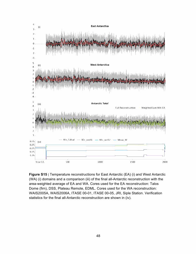
significant (p < 0.01) cooling trends from 166-1900 CE: -0.18 ± 0.02 °C ka-1 for East Antarctica, and -0.46 ± 0.02°C ka-1 for West Antarctica. The West Antarctic cooling trend may be partly due to elevation changes rather than cooling at a fixed elevation, although this is unlikely to account for the full magnitude of the trend66. The two reconstructions extending back to at least 166 CE that were then composited as an area-weighted average. Despite the different approach and the loss of pan-continental skill by only using each core in its own hemisphere, the reconstruction was very similar (Fig. S15).

Prior to 166 CE, the skill for the full Antarctic reconstruction decreases (Fig. S15), and the reconstruction errors increase. In this interval, for this reconstruction there is only one predictor in East Antarctica and one in the West. This very sparse sampling may introduce a geographical bias in the pre-166 CE reconstruction, with potential overrepresentation of West Antarctic changes. Therefore, because of the lack of skill and potential inadequacies in the network, we do not include this portion of the reconstruction in the main analysis.

38

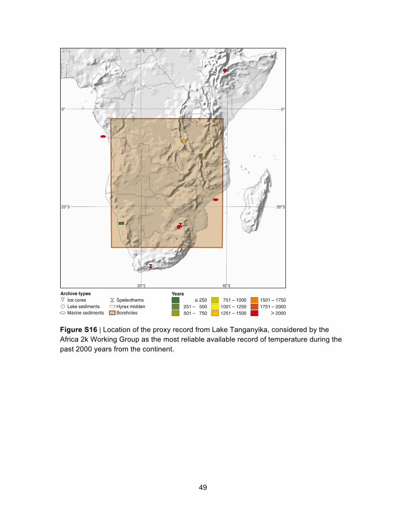
8. Africa The vast majority of paleoenvironmental records from Africa provide information about past moisture variability as opposed to temperature. The Africa 2k Working Group undertook an extensive literature review to identify studies from the continent in which paleotemperatures were either reconstructed or from which temperature could be estimated (Database S1 and Fig. S16). Paleotemperatures for the last two millennia have been reconstructed from sites in West, East and southern Africa. Each of the available studies were screened to determine their usefulness in assessing the continent-wide temperature variability67. Four criteria were used: (1) the robustness of the proxy used for determining paleotemperature; (2) the temporal resolution of the record; (3) the length of the record; and (4) the coherence of the record with other reconstructions of regional temperature change.

None of the records listed in Database S1 are annually resolved, and the majority is considered as only broad indicators of temperature change. The reconstructions for Lake Tanganyika68, Lake Malawi69, Cold Air Cave70,71 and Kilimanjaro72 display decadal- to centennial-scale variability. The interpretation of the Kilimanjaro δ18O record as a temperature indicator has been challenged73. However, a recent comparison with δ18O variability in nearby Lake Challa shows an out-of-phase relationship throughout the Holocene, suggesting that changes in total precipitation are not the dominant control on ice core δ18O (ref. 74). The δ18O temperature reconstructions from Cold Air Cave and Cango Cave on the south coast75 are also in question because the controls on δ18O variations in southernmost Africa are complex, and it remains unclear whether δ18O can be used reliably to reconstruct paleotemperatures in the region71.

Larger-scale temperature reconstructions have also been proposed from the Congo76 and Zambezi77 basins using the methylation index of branched tetraethers (MBT) and cyclisation ratio of branched tetraethers (CBT) based on branched glycerol dialkyl glycerol tetraethers (GDGTs). There is broad, first-order coherence between the Congo Basin record and global78,79 and extra-regional African paleotemperature trends80 over the last 20 ka. However, the Zambezi record is remarkable in that it is reported to indicate continental temperatures during the Younger Dryas cold reversal to be about 5°C higher than Holocene averages, and a decline (rather than increase) in temperatures of about 9°C during the glacial-interglacial transition. This suggests that the proxy may require further evaluation.

The reconstruction for Lake Tanganyika, which spans the period 500-2000 CE, is considered by the Working Group to be the highest resolution and most robust temperature reconstruction in Africa. It uses the TEX86 proxy, based on differences in the relative degree of cyclisation in GDGT molecules produced in the membranes of the aquatic Thaumarchaeota, which show a strong correlation with temperature in surface sediment and culture experiments68,80. The 20th century segment of the reconstructed lake-surface temperature record shows good agreement with instrumental data68. Furthermore, the main fluctuations in temperature since 1300 CE are coincident with, and of similar magnitude to, the lower resolution TEX86 reconstruction of lake-surface temperatures for Lake Malawi69,81. Whether the Lake Tanganyika record is

39

representative of continental temperature variability in not known. The coherence of the lake-surface temperature record with that of Lake Malawi suggests that it is at least representative of temperature variability in tropical east Africa. While the Working Group considers it problematic to extend the spatial representativeness of the record much beyond this region, the similarities observed in pollen-based temperature reconstructions from the Kuiseb River, Namibia82, the Ethiopian Highlands83 and Wonderkrater, South Africa84,85,86 and the borehole reconstructions presented by Huang et al.87 suggest that the large-lake records may reflect broader spatial trends.

40

Figure S7 | Arctic 2k regional domain with location of proxy records used for the temperature reconstruction. Instrumental target includes both land and ocean. Symbol shape indicates the proxy type and the color indicates the length of the record.

41

Figure S8 | Europe regional domain with locations of tree-ring and documentary records used for the temperature reconstruction. Instrumental target includes land area only. Symbol color indicates the length of the record.

42

Figure S9 | Asia 2k regional domain with locations of tree-ring records used for the temperature reconstruction. Instrumental target includes land area only. Symbol color indicates the length of the record.

43

Figure S10 | North America 2k regional domain with location of proxy records used for the temperature reconstruction. Instrumental target includes both land and ocean, but excludes the farthest northeastern cell centered at 52.5°N, 77.5°W. Symbol shape indicates the proxy type and the color indicates the length of the record. Symbols for pollen records are plotted at the centroid of ecoregions as delimited by Viau et al.44 .

44

Figure S11 | North America 2k decadal reconstruction (red), as explained in methods section above (reported in a different format in Fig. S2). Values are decadal means, with f=1/7 (~110 year) lowess filter to highlight low-frequency fluctuations. Dotted red line is the average for the entire period; variable shading represents the relative probability density for each decadal mean value from the uncertainty estimation process; narrow red lines denote 99% probability range associated with each decadal mean expected value reconstruction.

45

Figure S12 | South America 2k regional domain with location of proxy records used for the temperature reconstruction. Instrumental target includes land area only. Symbol shape indicates the proxy type and the color indicates the length of the record.

46

Figure S13 | Australasia 2k regional domain with location of proxy records used for the temperature reconstruction. Instrumental target includes both land and ocean. Symbol shape indicates the proxy type and the color indicates the length of the record

47

Figure S14 | Antarctic 2k regional domain with location of proxy records used for the temperature reconstruction. Instrumental target includes land area only. Symbol color indicates the length of the record.

48

Figure S15 | Temperature reconstructions for East Antarctic (EA) (i) and West Antarctic (WA) (i) domains and a comparison (iii) of the final all-Antarctic reconstruction with the area-weighted average of EA and WA. Cores used for the EA reconstruction: Talos Dome (firn), DSS, Plateau Remote, EDML. Cores used for the WA reconstruction: WAIS2005A, WAIS2006A, ITASE 00-01, ITASE 00-05, JRI, Siple Station. Verification statistics for the final all-Antarctic reconstruction are shown in (iv).

49

Figure S16 | Location of the proxy record from Lake Tanganyika, considered by the Africa 2k Working Group as the most reliable available record of temperature during the past 2000 years from the continent.

50

Table S5. Correlations for ice core 1 isotope time series with the instrumental target series.

Correlation interval 1957-

EAIS WAIS

including Pen

WAIS without

Pen

Antarctica total

Talos Dome (firn) 1995 0.24 0.09 0.10 0.21 DSS 2006 0.24 0.14 0.15 0.23 Plateau Remote 1991* 0.24 0.05 0.05 0.20 IND22/B 1994 -0.03 -0.25 -0.25 -0.08 DML05 1996 0.36 0.33 0.33 0.37 WD2005A 2005 0.14 0.47 0.46 0.23 WD2006A cal (WD2005A smooth**) 2005 0.13 0.51 0.51 0.24 ITASE00-01 2000 0.34 0.57 0.57 0.43 ITASE00-05 2000 0.30 0.12 0.13 0.27 James Ross Is 2006 -0.06 0.19 0.18 0.00 Siple Station 1991* 0.42 0.50 0.51 0.46

*With infill as described; **See Supplementary text; Pen = Peninsula

51

Supplementary Information References 1. http://www.ncdc.noaa.gov/paleo/paleo.html 2. http://www.pangaea.de/ 3. http://www.neotomadb.org/ 4. http://www.ncdc.noaa.gov/paleo/pages2k/pages-2k-network.html 5. http://hurricane.ncdc.noaa.gov/pls/paleox/f?p=514:1 6. http://www.ncdc.noaa.gov/paleo/data.html 7. Hanhijärvi, S., Tingley, M. P. & Korhola A. Pairwise comparisons to reconstruct mean

temperature in the arctic Atlantic region over the last 2000 years. Clim. Dyn. (in press) DOI: 10.1007/s00382-013-1701-4.

8. Li, B., Nuchka, D. W. & Ammann, C. M. The value of multiproxy reconstruction of past climate. J. Amer. Stat. Assoc. 105, 883-911(2010).

9. Jones, P. D. et al. Hemispheric and large-scale land-surface air temperature variations: An extensive revision and an update to 2010. J. Geophys. Res. 117, D05127 (2012).

10. Goosse, H. et al. Description of the Earth system model of intermediate complexity LOVECLIM version 1.2. Geosci. Model Dev. 3, 603–633 (2010).

11. Opsteegh, J. D., Haarsma, R. J., Selten, F. M. & Kattenberg, A. ECBilt: A dynamic alternative to mixed boundary conditions in ocean models. Tellus 50A, 348-367 (1998).

12. Goosse, H. & Fichefet T. Importance of ice-ocean interactions for the global ocean circulation: a model study. J. Geophys. Res. 104, 23337-23355 (1999).

13. Brovkin, V., Bendtsen, J., Claussen, M., Ganopolski, A., Kubatzki, C., Petoukhov, V. & Andreev, A. Carbon cycle, vegetation and climate dynamics in the Holocene: experiments with the CLIMBER-2 model. Global Biogeochem. Cycles 16, doi: 10.1029/2001GB001662 (2002).

14. Schmidt, G. A. et al. Climate forcing reconstructions for use in PMIP simulations of the last millennium (v1.0), Geosci. Model Dev. 4, 33-45 (2011).

15. Delaygue, G. & Bard, E. An Antarctic view of beryllium-10 and solar activity for the past millennium. Clim. Dynam. 36, 2201-2218 (2011).

16. Wang, Y. -M., Lean J. L. & Sheeley N. R. Modeling the Sun’s magnetic field and irradiance since 1713. Astrophys. J. 625, 522–538 (2005).

17. Berger, A. Long-term variations of daily insolation and Quaternary climatic changes. J. Atmosph. Sci. 35, 2363-2367 (1978).

18. Crowley, T. J., Zielinski, G., Vinther, B., Udisti, R., Kreutzs, K., Cole-Dia, J. & Castellano, E. Volcanism and the Little Ice Age. PAGES Newsletter 16, 22-23 (2008).

19. Pongratz, J., Reick, C. H., Raddatz, T. & Claussen, M. A reconstruction of global agricultural areas and land cover for the last millennium. Global Biogeochem. Cycles 22, GB3018 (2008).

20. Ramankutty N. & Foley J. A. Estimating historical changes in global land cover: croplands from 1700-1992. Global Biogeochem. Cycles 13, 997-1027 (1999).

21. Kaufman, D. S. et al. Recent warming reverses long-term Arctic cooling. Science 325, 1236-1239 (2009).

22. Brohan, P., Kennedy, J. J., Harris I., Tett, S. F. B. & Jones, P. D. Uncertainty estimates in regional and global observed temperature changes: A new data set from 1850. J. Geophys. Res. 111, D12106 (2006).

23. Bullmore, E. et al. Colored noise and computational inference in neurophysiological (fMRI) time series analysis: Resampling methods in time and wavelet domains. Hum. Brain Mapp. 12, 61 (2001).

52

24. Schneider, T. Analysis of incomplete climate data: Estimation of mean values and covariance matrices and imputation of missing values. J. Clim. 14, 853-871 (2001).

25. North, G. R., Moeng, F. J., Bell, T. L. & Cahalan, R. F. The latitude dependence of the variance of zonally averaged quantities. Mon. Weather Rev. 110, 319-326 (1982).

26. Esper, J., Cook, E. R., Krusic, P. J., Peters, K. & Schweingruber, F. H. Tests of the RCS method for preserving low-frequency variability in long tree-ring chronologies. Tree-Ring Res. 59, 81-98 (2003).

27. Esper, J. et al. Orbital forcing of tree-ring data. Nature Clim. Change, (2012), doi:10.1038/nclimate1589.

28. Briffa, K. R. et al. Fennoscandian summers from AD 500: temperature changes on short and long timescales, Clim. Dyn. 7, 111-119 (1992).

29. Grudd, H. Torneträsk tree-ring width and density AD 500-2004: A test of climatic sensitivity and a new 1500-year reconstruction of north Fennoscandian summers. Clim. Dyn. 31, 843-857 (2008).

30. Dobrovolný, P. et al. Monthly, seasonal and annual temperature reconstructions for central Europe derived from documentary evidence and instrumental records since AD 1500. Clim. Change 101, 69-107 (2010).

31. Mann, M. E. et al. Proxy-based reconstructions of hemispheric and global surface temperature variations over the past two millennia. Proc. Natl. Acad. Sci. U.S.A. 105, 13252-13257 (2008).

32. Jones, P. D. et al. High-resolution palaeoclimatology of the last millennium: A review of current status and future prospects. Holocene 19, 3-49 (2009).

33. McShane. B. B. & Wyner, A. J. A statistical analysis of multiple temperature proxies: are reconstructions of surface temperatures over the last 1000 years reliable? Ann. Appl. Statist. 5, 5-44 (2011).

34. Cook, E. R., Briffa, K. R. & Jones, P. D. Spatial regression methods in dendroclimatology: A review and comparison of two techniques. Int. J. Climatol. 14, 379-402 (1994).

35. Mitchell, T. D. & Jones, P. D. An improved method of constructing a database of monthly climate observations and associated high-resolution grids. Int. J. Clim. 25, 693-712 (2005).

36. Cook, E. R. et al. Asian monsoon failure and megadrought during the last millennium. Science 328, 486-489 (2010).

37. Cook, E. R., Meko, D. M., Stahle, D. W. & Cleaveland, M. K. Drought reconstructions for the continental United States. J. Clim. 12, 1145-1162 (1999).

38. Dai, A., Trenberth, K. E. & Qian, T. A global data set of Palmer Drought Severity Index for 1870-2002: Relationship with soil moisture and effects of surface warming. J. Hydrometeorol. 5, 1117-1130 (2004).

39. Cook, E. R., Briffa, K. R., Meko, D. M., Graybill, D. A. & Funkhouser, G. The segment length curse in long tree-ring chronology development for paleoclimatic studies. The Holocene 5, 229-237 (1995).

40. Gnanadesikan, R. Methods of Statistical Data Analysis of Multivariate Observations (John Wiley & Sons, New York, ed. 2, 1997).

41. Wahl, E. R. & Smerdon, J. E. Comparative performance of paleoclimate field and index reconstructions derived from climate proxies and noise-only predictors. Geophys. Res. Lett. 39, L06703 (2012).

42. http://www.ncdc.noaa.gov/paleo/treering.html 43. Mann M. E. et al. Global signatures and dynamical origins of the Little Ice Age and Medieval

Climate Anomaly. Science 326, 1256-1260 (2009). 44. Viau, A. E., Ladd, M. & Gajewski, K. The climate of North America during the past 2000 years

reconstructed from pollen data. Glob. Planet. Change 84-85, 75-83 (2012).

53

45. Neukom, R. et al. Multiproxy summer and winter surface air temperature field reconstructions for southern South America covering the past centuries. Clim. Dyn. 37, 35-51 (2011).

46. Neukom, R. & Gergis, J. Southern Hemisphere high-resolution palaeoclimate records of the last 2000 years. The Holocene 22, 501-524 (2012).

47. Reuter, J. et al. A new perspective on the hydroclimate variability in northern South America during the Little Ice Age. Geophys. Res. Lett. 36: L21706 (2009).

48. Le Quesne, C. Ancient Austrocedrus tree-ring chronologies used to reconstruct central Chile precipitation variability from A.D. 1200 to 2000. J. Clim. 19, 5731-5744 (2006).

49. Elbert, J. et al. Quantitative high-resolution winter (JJA) precipitation reconstruction from varved sediments of Lago Plomo 47°S, Patagonian Andes, AD 1530 - 2001. Holocene 22, 465-474 (2011).

50. Mundo, I., Roig Juñent, F., Villalba, R., Kitzberger, T. & Barrera, M. Araucaria araucana tree-ring chronologies in Argentina: spatial growth variations and climate influences. Trees-Struct. Funct. 26, 443-458 (2012).

51. Villalba, R. et al. Large-scale temperature changes across the southern Andes: 20th-century variations in the context of the past 400 years. Clim. Change 59, 177-232 (2003).

52. Gergis, J. et al. Evidence of unusual late 20th century warming from an Australasian temperature reconstruction spanning the last millennium. J. Clim. (in review).

53. Neukom, R. et al. Multi-centennial summer and winter precipitation variability in southern South America. Geophys. Res. Lett. 37, L14708 (2010).

54. Rayner, N. A. et al. Improved analyses of changes and uncertainties in sea surface temperature measured in situ since the mid-nineteenth century: The HadSST2 dataset. J. Clim. 19, 446-469 (2006).

55. Phipps, S. J. et al. Paleoclimate data-model comparison and the role of climate forcings over the past 1500 years. J. Clim. (in revision).

56. Scherrer, S. C. & Appenzeller, C. Swiss Alpine snow pack variability: major patterns and links to local climate and large-scale flow. Clim. Res. 32, 187-199 (2006).

57. Gallant, A. J. E. & Gergis, J. An experimental streamflow reconstruction for the River Murray, Australia, 1783–1988. Water Resour. Res. 47, W00G04 (2011).

58. Luterbacher, J. et al. Reconstruction of sea level pressure fields over the Eastern North Atlantic and Europe back to 1500. Clim. Dyn. 18, 545-561 (2002).

59. Cook, E. R. & Kairiukstis, L. Methods of Dendrochronology (Kluwer Academic Publishers, Dordrecht, 1990).

60. Steig, E. J. et al. Warming of the Antarctic ice-sheet surface since the 1957 International Geophysical Year. Nature 457, 459-462 (2009).

61. Vinther, B. M. A synchronized dating of three Greenland ice cores throughout the Holocene, J. Geophys. Res. 111, D13102 (2006).

62. Plummer, C. T. et al. An independently dated 2000-yr volcanic record from Law Dome, East Antarctica, including a new perspective on the dating of the 1450s CE eruption of Kuwae, Vanuatu. Clim. Past 8, 1929-1940 (2012).

63. Sigl, M. J. R. et al. A new bi-polar ice core record of volcanism from WAIS Divide and NEEM: Implications for climate forcing during the last 2000 years. J. Geophys. Res. (accepted).

64. Schneider, D. P. et al. Antarctic temperatures over the past two centuries from ice cores. Geophys. Res. Lett. 33, L16707 (2006).

65. Rousseeuw, P. J., Least median of squares regression. J. Am. Stat. Assoc. 79, 871-880 (1984).

66. Fegyveresi, J. M. et al. Late-Holocene climate evolution at the WAIS Divide site, West Antarctica: bubble number-density estimates. J. Glaciol. 57(204), 629-638 (2011).

54

67. Nicholson, S. E. et al. Temperature variability over Africa during the last 2000 years. Holocene (in press) DOI:10.1177/0959683613483618.

68. Tierney, J. E. et al. Late-twentieth-century warming in Lake Tanganyika unprecedented since AD 500. Nature Geosci. 3, 422-425 (2010).

69. Powers, L. A. et al., Large temperature variability in the southern African tropics since the Last Glacial Maximum. Geophys. Res. Lett. 32, L08706 (2005).

70. Lee-Thorp, J. A. et al. Rapid climate shifts in the southern African interior throughout the mid to late Holocene. Geophys. Res. Lett. 28, (2001).

71. Holmgren, K. et al. Persistent millennial-scale climatic variability over the past 25,000 years in Southern Africa. Quat. Sci. Rev. 22, 2311-2326 (2003).

72. Thompson, L. G. et al. Kilimanjaro ice core records: evidence of Holocene climate change in tropical Africa. Science 298, 589-593 (2002).

73. Gasse, F. Kilimanjaro’s secrets revealed. Science 298, 548-549 (2002). 74. Barker, P. A. et al. A 14,000-year oxygen isotope record from diatom silica in two alpine lakes

on Mt. Kenya. Science 292, 2307-2310 (2001). 75. Talma, A. S. & Vogel, J. C. Late Quaternary paleotemperatures derived from a speleothem

from Cango Caves, Cape Province, South Africa. Quat. Res. 37, 203-213 (1992). 76. Weijers, J. W. H., Schefuß, E., Schouten, S. & Sinninghe Damsté, J. S. Coupled thermal and

hydrological evolution of tropical Africa over the last deglaciation. Science 315, 1701-1704 (2007).

77. Schefuß, E., Kuhlmann, H., Mollenhauer, G., Prange, M. & Pätzold J. Forcing of wet phases in southeast Africa over the past 17,000 years. Nature 480, 509-512 (2011).

78. Dansgaard, W. et al., Evidence for general instability of past climate from a 250 kyr ice core record. Nature 364, 218-220 (1993).

79. EPICA Community Members. Eight glacial cycles from an Antarctic ice core. Nature 429, 623-628 (2004).

80. Tierney, J. E. et al. Northern Hemisphere controls on tropical southeast African climate during the past 60,000 years. Science 322, 252-255 (2008).

81. Powers, L. A. et al. Organic geochemical records of environmental variability in Lake Malawi during the last 700 years, Part I: the TEX86 temperature record. Palaeogeogr. Palaeoclimatol. Palaeoecol. 303, 133-139 (2011).

82. Scott, L. Palynology of hyrax middens: 2000 years of palaeoenvironmental history in Namibia. Quat. Int. 33, 73-79 (1996).

83. Bonnefille, R. & Umer, M. Pollen inferred climatic fluctuations in Ethiopia during the last 3000 years. Palaeogeogr. Palaeoclimatol. Palaeoecol. 109, 331-343 (1994).

84. Scott, L. Vegetation history and climate in the Savanna biome South Africa since 190,000 ka: a comparison of pollen data from the Tswaing Crater (the Pretoria Saltpan) and Wonderkrater. Quat. Int. 57-58, 215-223 (1999).

85. Scott, L., Holmgren, K., Talma, A. S., Woodborne, S. & Vogel, J. C. Age interpretation of the Wonderkrater spring sediments and vegetation change in the Savanna Biome, Limpopo province, South Africa. S. Afr. J. Sci. 99, 484-488 (2003).

86. Thackeray, J. F. Calibration of temperature indices from a late Quaternary terrestrial sequence at Wonderkrater, South Africa. Quat. Int. 57-58, 225-227 (1999).

87. Huang, S., Pollack, H. N. & Shen, P. -Y. Temperature trends over the past five centuries reconstructed from borehole temperatures. Nature 403, 756-758 (2000).