Supplementary Information for

Identification of the Current Path for a Conductive

Molecular Wire on a Tripodal Platform

M. A. Karimi,a S. G. Bahoosh,a M. Valášek, b M. Bürkle, c M. Mayor, b,d,e F. Pauly a and E. Scheer* a a Department of Physics, University of Konstanz, 78457 Konstanz, Germany Email: elke.scheer@uni-konstanz.de b Karlsruhe Institute of Technology (KIT), Institute of Nanotechnology, P.O. Box 3640, 76021

Karlsruhe, Germany c Nanosystem Research Institute (NRI) ‘RICS’, National Institute of Advanced Industrial Science

and Technology (AIST), Tsukuba, Ibaraki 305-8568, Japan d Department of Chemistry, University of Basel, 4056 Basel, Switzerland e Lehn Institute of Functional Materials (LIFM), Sun Yat-Sen University (SYSU), Xingang Rd. W.,

Guangzhou, China

1. Synthesis data, NMR spectra of the compounds 2

2. Distance calibration 17

3. Electrical circuit 18

4. Vibrational mode assignment 18

5. Control experiments 18

6. Additional examples of IET spectra 20

7. Theory 21

References 24

1

Electronic Supplementary Material (ESI) for Nanoscale.This journal is © The Royal Society of Chemistry 2016

1. Synthesis data, NMR spectra of the compounds Our synthetic strategy is described in the Methods section. Here we summarize the materials, equipment and characterization measurements and show the NMR data of all target molecules.

Materials. All starting materials and reagents were obtained from commercial suppliers and used without further purification. TLC was performed on Silica gel 60 F254 plates, spots were detected by fluorescence quenching under UV light at 254 nm, and/or staining with appropriate solutions (anisaldehyde, phosphomolybdic acid, KMnO4). Column chromatography was performed on silica gel 60 (0.040-0.063 mm). All experimental manipulations with anhydrous solvents were carried out in flame-dried glassware under an inert atmosphere of argon. Degassed solvents were obtained by three cycles of the freeze-pump-thaw. Tetrahydrofurane and dioxane were dried and distilled from sodium/benzophenone under argon atmosphere. Dichlormethane and triethylamine were dried and distilled from CaH2 under argon atmosphere. 4-Bromo-1-[2-(trimethylsilyl)ethylsulphanyl]benzene (1),S1,S2 2-bromo-7-iodo-9H-fluorene (8),S3 and 2-bromo-7-iodo-3’,6’-bis[2-(trimethylsilyl)ethylsulfanyl]-9,9’-spirobifluorene (4)S3 were prepared according to published procedures.

Equipment and measurements. All NMR spectra were recorded at 25 °C in CDCl3. 1H NMR (500.16 MHz) spectra were referenced to the solvent residual proton signal (CDCl3, δH = 7.24 ppm). 13C NMR (125.78 MHz) spectra with total decoupling of protons were referenced to the solvent (CDCl3, δC = 77.23 ppm). For correct assignment of both 1H and 13C NMR spectra, the 1H-1H COSY, 13C DEPT-135, HSQC and HMBS experiments were performed. EI MS spectra were recorded with a GC/MS instrument (samples were dissolved in diethyl ether, chloroform or introduced directly using direct injection probes DIP, DEP) and m/z values are given along with their relative intensities (%) at an ionizing voltage of 70 eV. IR spectra were measured in KBr pellets. Analytical samples were dried at 40 to 100 °C under reduced pressure (10-2 mbar). Melting points were measured with a melting point apparatus and are not corrected. Elemental analyses were obtained using an elemental analyser.

4-[(Trimethylsilyl)ethynyl]-1-[2-(trimethylsilyl)ethylsulfanyl]benzene (2).S4 A 100 mL Schlenk flask was charged with 4-bromo-1-[2-(trimethylsilyl)ethylsulphanyl]benzene (1) (2.0 g, 6.9 mmol), PdCl2(PPh3)2 (350 mg, 0.5 mmol), CuI (190 mg, 1.0 mmol) under argon, and dry triethylamine (40 mL) was added. Then trimethylsilylacetylene (1.0 g, 1.5 mL, 10.4 mmol) was added, and the mixture was stirred at 50 °C for 4 h and finally at 80 °C for an additional 3 h. The reaction mixture was treated with diethyl ether (200 mL) and the precipitate was filtered through a pad of silica gel (20 g, diethyl ether), and the filtrate was concentrated in vacuo. The residue was purified by column chromatography on silica gel (800 g, hexane) to afford the title compound 2 (2.02 g) as a light yellow oil which solidified upon standing in 95% yield (Rf = 0.34, Hex:CH2Cl2 = 50:1): mp 46-47 °C. 1H NMR (500 MHz, CDCl3) δ ppm: 0.03 (s, 9H, CH3, TMSE), 0.23 (s, 9H, CH3, TMS-C≡C), 0.90 (m, 2H, CH2Si), 2.94 (m, 2H, SCH2), 7.17 (dd, J = 8.5 Hz, J = 2 Hz, 2H, C2H, C6H), 7.35 (dd, J = 8.5 Hz, J = 2 Hz, 2H, C3H, C5H). 13C NMR (125.8 MHz, CDCl3) δ ppm: -1.6 (CH3, TMSE), 0.2 (CH3, TMS), 16.8 (CH2Si), 29.1 (SCH2), 94.5 (C2’), 105.1 (C1’), 120.1 (C4), 127.9 (C2H, C6H), 132.4 (C3H, C5H), 138.8 (C1). IR (KBr) ν cm-1 3078 (w) and 3028 (w, ν(=CH)), 2953 (vs)

2

and 2921 (s, νas(CH3)), 2894 (w, νs(CH3)), 2157 (vs, ν(C≡C)), 1589 (s, ν(CC), Ph), 1489 (vs), 1429 (m), 1417 (m), 1397 (m), 1246 (bs, δs(CH3), TMS), 1227 (m), 1160 (m), 1089 (m), 1012 (s), 862 (vs) and 844 (bs, δas(CH3), TMS), 759 (s), 708 (m), 694 (m, vas(SiC3), TMS), 677 (m), 533 (m). EI MS m/z (%) 306 (36, M+), 278 (8), 263 (64), 190 (17), 124 (16), 101 (24), 73 (100). Anal. calcd. for C16H26SSi2 (306.61): C, 62.68; H, 8.55. Found: C, 62.73; H, 8.57.

4-Ethynyl-1-[2-(trimethylsilyl)ethylsulfanyl]benzene (3).S4 In a 100 mL flask, the silylated acetylene 2 (1.6 g, 5.2 mmol) was dissolved in the mixture of THF (30 mL) and methanol (30 mL). Potassium carbonate (7.2 g, 52 mmol) was added, and the suspension was vigorously stirred at room temperature for 20 h. The reaction mixture was diluted with diethyl ether (100 mL), filtered through a pad of Celite (diethyl ether), and the remaining solution concentrated under reduced pressure. The crude product was treated with the mixture of diethyl ether and hexane (1:1, 100 mL), and passed through a short pad of silica gel (100 g, diethyl ether:hexane = 1:1). After evaporation and drying under vacuo at room temperature, the title compound 3 (1.2 g) was isolated as a light yellow oil in 98% yield (Rf = 0.30, hexane). 1H NMR (500 MHz, CDCl3) δ ppm: 0.03 (s, 9H, CH3, TMSE), 0.91 (m, 2H, CH2Si), 2.95 (m, 2H, SCH2), 3.05 (s, 1H, CH), 7.19 (dd, J = 7 Hz, J = 2 Hz, 2H, C2H, C6H), 7.37 (dd, J = 7 Hz, J = 2 Hz, 2H, C3H, C5H). 13C NMR (125.8 MHz, CDCl3) δ ppm: -1.6 (CH3, TMSE), 16.8 (CH2Si), 29.1 (SCH2), 83.7 (C1’, C2’), 119.0 (C4), 127.9 (C2H, C6H), 132.6 (C3H, C5H), 139.3 (C1). IR (KBr) ν cm-1 3295 (m, ν(≡CH)), 3028 (vw, ν(=CH)), 2953 (m) and 2921 (m, νas(CH3)), 2890 (w, νs(CH3)), 2108 (m, ν(C≡C)), 1593 (m, ν(CC), Ph), 1489 (s), 1418 (w), 1399 (w), 1250 (vs, δs(CH3), TMS), 1164 (w), 1090 (m), 1015 (m), 859 (vs) and 840 (bs, δas(CH3), TMS), 753 (w), 693 (m, vas(SiC3), TMS), 653 (w), 529 (m). EI MS m/z (%) 234 (43, M+), 206 (80), 191 (78), 115 (14), 101 (37), 89 (22), 73 (100), 45 (17). Anal. calcd. for C13H18SSi (234.43): C, 66.60; H, 7.74. Found: C, 66.76; H, 7.65.

2-Bromo-7-({4-[2-(trimethylsilyl)ethylsulfanyl]phenyl}ethynyl)-3’,6’-bis[2-(trimethylsilyl)ethylsulfanyl]-9,9’-spirobifluorene (5). An argon-flushed 25 mL Schlenk flask was charged with spirobifluorene 4S3 (300 mg, 382 μmol), PdCl2(PPh3)2 (13 mg, 19 μmol), and CuI (7 mg, 38 μmol), and dry triethylamine (18 mL) was added. The flask was cooled to approx. 0 °C with a water-ice bath and acetylene derivative 3 (98 mg, 420 μmol) was added under argon. The reaction mixture was stirred at room temperature for 12 h. The completion of the reaction was checked by TLC (Hex:EtOAc = 40:1). The reaction mixture was treated with diethyl ether (50 mL) and the precipitate was filtered through a pad of silica gel (10 g, diethyl ether), and the filtrate was concentrated in vacuo. The residue was purified by column chromatography on silica gel (600 g, hexane:EtOAc equal to 40:1) to provide the desired product 5 (327 mg) as a light yellow foamy solid in 96% yield (Rf = 0.24; Hex:EtOAc = 40:1): mp 64-65 °C. 1H NMR (500 MHz, CDCl3) δ ppm: 0.02 (s, 9H, CH3), 0.06 (s, 18H, CH3), 0.90 (m, 2H, CH2Si), 0.99 (m, 4H, CH2Si), 2.93 (m, 2H, SCH2), 3.03 (m, 4H, SCH2), 6.63 (d, J = 8 Hz, 2H, C1’H, C8’H), 6.86 (d, J = 7 Hz, 2H, C1H, C8H), 7.07 (dd, J = 8 Hz, J = 1.5 Hz, 2H, C2’H, C7’H), 7.15 (dd, J = 8.5 Hz, J = 1.5 Hz, 2H, C3’’H, C5’’H), 7.29 (dd, J = 8.5 Hz, J = 1.5 Hz, 2H, C2’’H, C6’’H), 7.48 (dd, J = 8 Hz, J = 1.5 Hz, 1H, C3H), 7.51 (dd, J = 8 Hz, J = 1.5 Hz, 1H, C6H), 7.66 (d, J = 8 Hz, 1H, C4H), 7.73 (d, J = 1.5 Hz, 2H, C4’H, C5’H), 7.75 (d, J = 8.5 Hz, 1H, C5H). 13C NMR (125.8 MHz, CDCl3) δ ppm: -1.6 (CH3), -1.5 (2 × CH3), 16.8 (CH2Si), 17.1 (2 × CH2Si), 29.1 (SCH2), 30.0 (2 × SCH2), 65.2 (C9), 89.9 (C1’), 90.3 (C2’), 119.9 (C1’’), 120.3 (C5H), 120.5 (C4’H, C5’H), 121.8 (C4H), 122.2 (C2), 123.1 (C7),

3

124.6 (C1’H, C8’H), 127.4 (C1H), 127.6 (C8H), 127.9 (C3’’H, C5’’H), 128.8 (C2’H, C7’H), 131.4 (C3H), 131.8 (C6H), 131.9 (C2’’H, C6’’H), 137.9 (C3’, C6’, C2), 138.7 (C4’’), 140.2 (C11), 140.8 (C12), 142.1 (C11’, C12’), 145.4 (C10’, C13’), 148.5 (C13), 150.9 (C10). IR (KBr) ν cm-1 3052 (w, ν(=CH)), 2951 (m) and 2916 (m, νas(CH2, CH3)), 2893 (w, νs(CH2, CH3)), 2211 (vw, ν(C≡C)), 1596 (m) and 1559 (w, ν(CC), Ph), 1495 (m), 1455 (w), 1417 (m), 1402 (w), 1259 (s), 1249 (vs, δs(CH3), TMS), 1162 (m), 1123 (vw), 1086 (m), 1063 (w), 1007 (m), 956 (w), 858 (vs) and 840 (vs, δas(CH3), TMS), 816 (vs), 753 (m), 693 (m, vas(SiC3), TMS), 638 (m), 530 (w). EI MS m/z (%) 893 (1), 890 (1, M+), 808 (1), 806 (1), 101 (7), 84 (6), 73 (100), 49 (7), 44 (34). Anal. calcd. for C48H55BrS3Si3 (892.31): C, 64.61; H, 6.21. Found: C, 64.85; H, 6.32.

2,3’,6’-Tris[2-(trimethylsilyl)ethylsulfanyl]-7-({4-[2-(trimethylsilyl)ethylsulfanyl]phenyl}-ethynyl)-9,9’-spirobifluorene (6). A dry 25 mL round bottom flask was charged with spirobifluorene 5 (250 mg, 280 μmol), Xantphos (8 mg, 14 μmol), Pd2(dba)3 (7 mg, 7 μmol), and dry dioxane (16 mL). The tube was evacuated under vacuum and refilled with argon three times. Then N,N-diisopropylethylamine (110 mg, 145 μL, 0.85 mmol), and 2-(trimethylsilyl)ethanethiol (75 mg, 90 μmol, 0.56 mmol) were added under argon and the tube was quickly capped with a rubber septum. The reaction mixture was heated at 100 °C for 14 h. The completion of the reaction was checked by TLC (Hex:EtOAc = 20:1). After cooling, the reaction mixture was diluted with diethyl ether (50 mL), filtered through a pad of silica gel (15 g, diethyl ether), and the filtrate was concentrated in vacuo. The crude product was purified by column chromatography on silica gel (300 g, hexane:EtOAc equal to 40:1) to provide the title compound 6 (254 mg) as a light yellow foamy solid in 96% yield (Rf = 0.22, Hex:EtOAc = 40:1). 1H NMR (500 MHz, CDCl3) δ ppm: -0.10 (s, 9H, CH3

(→2)), 0.02 (s, 9H, CH3(→4”)), 0.06 (s, 18H,

CH3(→3’), CH3

(→6’)), 0.76 (m, 2H, CH2Si(→2)), 0.90 (m, 2H, CH2Si(→4”)), 0.99 (m, 4H, CH2Si(→3’), CH2Si(→6’)), 2.79 (m, 2H, SCH2

(→2)), 2.93 (m, 2H, SCH2(→4”)), 3.03 (m, 4H, SCH2

(→3’), SCH2(→6’)), 6.62

(d, J = 1.5 Hz, 1H, C1H), 6.65 (d, J = 8 Hz, 2H, C1’H, C8’H), 6.86 (d, J = 1 Hz, 1H, C8H), 7.05 (dd, J = 8 Hz, J = 1.5 Hz, 2H, C2’H, C7’H), 7.16 (dd, J = 8 Hz, J = 1.5 Hz, 2H, C3’’H, C5’’H), 7.26 (dd, J = 8 Hz, J = 1.5 Hz, 1H, C3H), 7.29 (dd, J = 8 Hz, J = 1.5 Hz, 2H, C2’’H, C6’’H), 7.50 (dd, J = 8 Hz, J = 1 Hz, 1H, C6H), 7.71 (d, J = 8 Hz, 1H, C4H), 7.72 (d, J = 8 Hz, 1H, C5H), 7.73 (d, J = 1.5 Hz, 2H, C4’H, C5’H). 13C NMR (125.8 MHz, CDCl3) δ ppm: -1.7 (CH3

(→2)), -1.6 (CH3(→4”)), -1.5 (CH3

(→3’), CH3(→6’)), 16.8

(CH2Si(→4”)), 16.9 (CH2Si(→2)), 17.1 (CH2Si(→3’), CH2Si(→6’)), 29.1 (SCH2(→4”)), 29.4 (SCH2

(→2)), 30.0 (SCH2

(→3’), SCH2(→6’)), 65.2 (C9), 89.9 (C1’), 90.1 (C2’), 119.97 (C5H), 120.04 (C1’’), 120.5 (C4’H, C5’H),

120.8 (C4H), 122.4 (C7), 124.2 (C1H), 124.7 (C1’H, C8’H), 127.3 (C8H), 127.9 (C3’’H, C5’’H), 128.6 (C3H), 128.8 (C2’H, C7’H), 131.7 (C6H), 131.9 (C2’’H, C6’’H), 137.6 (C3’, C6’, C2), 138.5 (C11), 138.9 (C4’’), 141.5 (C12), 142.1 (C11’, C12’), 146.1 (C10’, C13’), 148.5 (C13), 149.6 (C10). IR (KBr) ν cm-1 3058 (w) and 3032 (w, ν(=CH)), 2950 (m) and 2917 (w, νas(CH2, CH3)), 2851 (w, νs(CH2, CH3)), 2211 (vw, ν(C≡C)), 1597 (m) and 1562 (w, ν(CC), Ph), 1494 (m), 1456 (m), 1415 (m), 1248 (vs, δs(CH3), TMS), 1162 (m), 1122 (w), 1085 (m), 1010 (m), 960 (vw), 859 (vs) and 839 (vs, δas(CH3), TMS), 815 (s), 751 (m), 692 (m, vas(SiC3), TMS), 638 (m), 523 (w). EI MS m/z (%) 944 (3, M+), 101 (3), 86 (60), 84 (85), 73 (100), 51 (26), 49 (77). Anal. calcd. for C53H68S4Si4 (945.71): C, 67.31; H, 7.25. Found: C, 67.49; H, 7.16.

S,S’,S”-(7-{[4-(Acetylsulfanyl)phenyl]ethynyl}-9,9’-spirobifluorene-2,3’,6’-triyl] tris(thio-acetate) (7). In a 50 mL Schlenk flask, spirobifluorene 6 (220 mg, 230 μmol) was dissolved in the

4

mixture of dry dichloromethane (30 mL) and acetyl chloride (3 mL), and put under argon. The solution was treated with AgBF4 (358 mg, 1.84 mmol) and a violet suspension was stirred at room temperature for 4 h. The completion of the reaction was checked by TLC (Hex:EtOAc = 3:1). The reaction mixture was cooled to 0 °C, diluted with dichloromethane (30 mL) and slowly treated with water (20 mL). The precipitate was filtered through a pad of Celite (CH2Cl2), extracted with water (30 mL), brine (30 mL) and dried with magnesium sulphate. The solution was passed through a pad of silica gel (10 g, CH2Cl2), and the filtrate was concentrated in vacuo. The crude product was purified by column chromatography on silica gel (500 g, hexane: EtOAc equal to 3:1) to provide thioacetate 7 (120 mg) as a yellow solid in 73% yield (Rf = 0.24, Hex:EtOAc = 3:1): mp 160-162 °C. 1H NMR (500 MHz, CDCl3) δ ppm: 2.31 (s, 3H, CH3

(→4”)), 2.39 (s, 3H, CH3

(→2)), 2.44 (s, 6H, CH3(→3’), CH3

(→6’)), 6.78 (d, J = 1 Hz, 1H, C1H), 6.79 (d, J = 8 Hz, 2H, C1’H, C8’H), 6.91 (d, J = 1 Hz, 1H, C8H), 7.18 (dd, J = 7.5 Hz, J = 1.5 Hz, 2H, C2’H, C7’H), 7.31 (dd, J = 8 Hz, J = 1 Hz, 2H, C3’’H, C5’’H), 7.43 (dd, J = 8 Hz, J = 1 Hz, 2H, C2’’H, C6’’H), 7.45 (dd, J = 8 Hz, J = 2 Hz, 1H, C3H), 7.55 (dd, J = 8 Hz, J = 1.5 Hz, 1H, C6H), 7.81 (d, J = 8 Hz, 1H, C5H), 7.86 (d, J = 8 Hz, 1H, C4H), 7.87 (d, J = 1.5 Hz, 2H, C4’H, C5’H). 13C NMR (125.8 MHz, CDCl3) δ ppm: 30.33 (CH3

(→4”)), 30.46 (CH3(→2)), 30.48 (CH3

(→3’), CH3(→6’)), 65.6 (C9), 90.0 (C2’), 91.2 (C1’), 120.8 (C5H),

121.2 (C4H), 123.3 (C7), 124.5 (C1’’), 125.1 (C1’H, C8’H), 126.7 (C4’H, C5’H), 127.7 (C8H), 128.20 (C4’’), 128.27 (C2), 128.32 (C3’, C6’), 130.1 (C1H), 132.2 (C6H), 132.3 (C2’’H, C6’’H), 134.3 (C3’’H, C5’’H), 134.5 (C2’H, C7’H), 135.1 (C3H), 141.2 (C12), 142.1 (C11’, C12’), 142.4 (C11), 148.3 (C13), 148.7 (C10), 149.1 (C10’, C13’), 193.7 (CO(→4”)), 193.8 (CO(→2)), 194.0 (CO(→3’), CO(→6’)). IR (KBr) ν cm-1

3057 (vw, ν(=CH)), 2924 (vs, νas(CH3)), 2854 (w, νs(CH3)), 2212 (vw, ν(C≡C)), 1706 (vs, ν(C=O)), 1597 (m, ν(CC), Ph), 1494 (s), 1455 (s), 1386 (bs), 1352 (m), 1119 (vs), 1051 (w), 948 (s), 876 (m), 822 (s), 700 (w), 640 (m), 615 (s), 551 (w), 417 (w). EI MS m/z (%) 712 (5, M+), 670 (18), 628 (9), 586 (7), 544 (5), 164 (6), 84 (100), 51 (25), 49 (78), 43 (46). Anal. calcd. for C41H28O4S4 (712.91): C, 69.08; H, 3.96. Found: C, 69.35; H, 3.74.

2-Bromo-7-iodo-9,9-dimethylfluorene (9). In a 250 mL Schlenk flask 2-bromo-7-iodo-9H-fluorene 8S3 (2 g, 5.39 mmol) was dissolved in anhydrous THF (80 mL) under argon. The reaction mixture was cooled to 0 °C and potassium tert-butoxide (730 mg, 6.5 mmol) was added to afford a red solution. After 0.5 h, followed by methylation with methyl iodide (925 mg, 0.41 mL, 6.5 mmol), the reaction was stirred at room temperature for 1 h, then again cooled to 0 °C and potassium tert-butoxide (730 mg, 6.5 mmol) was added. Methyl iodide (925 mg, 0.41 mL, 6.5 mmol) was added after 0.5 h and the reaction mixture was stirred at room temperature overnight to afford a pink suspension. After quenching with water, a red solution was diluted with diethyl ether (100 mL) and the organic layer was subsequently washed with water (150 mL), NH4Cl (100 mL, 10% in water), Na2SO3 (100 mL, 10% in water), brine (100 mL), and dried with magnesium sulphate. After filtration, followed by solvent removal at reduced pressure, the residue was purified by column chromatography on silica gel (800 g, hexane) to provide 1.91 g of a white solid in 89% yield (Rf = 0.33, hexane): mp 185 °C. 1H NMR (500 MHz, CDCl3) δ ppm: 1.44 (s, 6H, CH3), 7.41 (d, J = 8 Hz, 1H, C5H), 7.44 (dd, J = 8 Hz, J =2 Hz, 1H, C3H), 7.52 (d, J = 2 Hz, 1H, C1H), 7.53 (d, J = 7 Hz, 1H, C4H), 7.63 (dd, J = 8 Hz, J =1.5 Hz, 1H, C6H), 7.73 (d, J = 1 Hz, 1H, C8H). 13C NMR (125.8 MHz, CDCl3) δ ppm: 27.1 (CH3), 47.5 (C9), 93.2 (C7), 121.7 (C4H), 121.8 (C2), 122.0 (C5H), 126.4 (C1H), 130.5 (C3H), 132.3 (C8H), 136.4 (C6H), 137.4 (C11), 138.0 (C12), 155.3

5

(C10), 155.6 (C13). IR (KBr) ν cm-1 3055 (vw) and 3021 (vw, ν(=CH)), 2958 (s) and 2919 (m, νas(CH3)), 2862 (m, νs(CH3)), 1594 (w) and 1573 (w, ν(CC), Ph), 1463 (m), 1448 (m), 1436 (m), 1397 (s), 1261 (s), 1128 (m), 1082 (m), 1054 (s), 1000 (m), 934 (w), 869 (s), 824 (m) and 793 (s, ν(CH)), 730 (s), 661 (m), 593 (m), 436 (s). EI MS m/z (%) 400 (96), 398 (100, M+), 385 (48), 383 (48), 319 (11), 304 (23), 258 (25), 256 (25), 192 (28), 176 (77), 151 (24), 95 (16), 88 (68), 75 (17). Anal. calcd. for C15H12BrI (399.07): C, 45.15; H, 3.03. Found: C, 45.23; H, 3.07.

2-Bromo-7-({4-[2-(trimethylsilyl)ethylsulfanyl]phenyl}ethynyl)-9,9-dimethylfluorene (10). The product was prepared according to the method described for the preparation of spirobifluorene 5, starting from fluorene 9 (0.4 g, 1 mmol), acetylene derivative 3 (260 mg, 1.1 mmol), PdCl2(PPh3)2 (39 mg, 55 μmol), and CuI (21 mg, 110 μmol) in dry triethylamine (30 mL). The reaction mixture was stirred at 0 °C for 2 h, then allowed to warm to room temperature and stirred for an additional 4 h under argon atmosphere. The crude product was purified by column chromatography on silica gel (800 g, hexane:EtOAc equal to 50:1 or Hex:CH2Cl2 equal to 5:1) to provide the desired product 10 (470 mg) as a light yellow solid in 93% yield (Rf = 0.26; Hex:EtOAc = 50:1): mp 162-163 °C. 1H NMR (500 MHz, CDCl3) δ ppm: 0.04 (s, 9H, CH3), 0.94 (m, 2H, CH2Si), 1.47 (s, 6H, CH3), 2.98 (m, 2H, SCH2), 7.23 (dd, J = 6.5 Hz, J = 2 Hz, 2H, C3’’H, C5’’H), 7.44 (dd, J = 6.5 Hz, J = 2 Hz, 2H, C2’’H, C6’’H), 7.45 (dd, J = 7 Hz, J = 1.5 Hz, 1H, C3H), 7.49 (dd, J = 8 Hz, J = 1.5 Hz, 1H, C6H), 7.53-7.57 (m, 3H, C1H, C8H, C4H), 7.63 (d, J = 8 Hz, 1H, C5H). 13C NMR (125.8 MHz, CDCl3) δ ppm: -1.5 (CH3), 16.8 (CH2Si), 27.1 (CH3

(→9)), 29.2 (SCH2), 47.3 (C9), 89.9 (C2’), 90.5 (C1’), 120.25 (C5H), 120.27 (C1’’), 121.7 (C2), 121.9 (C4H), 122.4 (C7), 126.1 (C8H), 126.4 (C1H), 128.1 (C3’’H, C5’’H), 130.5 (C3H), 131.1 (C6H), 132.1 (C2’’H, C6’’H), 137.8 (C11), 138.5 (C4’’), 138.6 (C12), 153.5 (C13), 156.1 (C10). IR (KBr) ν cm-1 3066 (w) and 3022 (w, ν(=CH)), 2953 (m) and 2919 (m, νas(CH2, CH3)), 2893 (m) and 2856 (m, νs(CH2, CH3)), 1592 (m, ν(CC), Ph), 1495 (s), 1482 (m), 1465 (m), 1449 (m), 1402 (s), 1260 (m), 1248 (s, δs(CH3), TMS), 1169 (w), 1146 (w), 1087 (s), 1075 (w), 1014 (m), 1005 (m), 943 (w), 862 (s) and 832 (s, δas(CH3), TMS), 806 (vs), 766 (m), 733 (m), 692 (m, vas(SiC3), TMS), 516 (m), 466 (m). EI MS m/z (%) 506 (22), 504 (20, M+), 478 (19), 476 (17), 309 (6), 276 (7), 176 (9), 101 (13), 73 (100), 45 (11). Anal. calcd. for C28H29BrSSi (505.59): C, 66.52; H, 5.78. Found: C, 66.39; H, 5.86.

2-[2-(Trimethylsilyl)ethylsulfanyl]-7-({4-[2-(trimethylsilyl)ethylsulfanyl]phenyl}ethynyl)-9,9-dimethylfluorene (11). The desired product was prepared according to the method described for the preparation of spirobifluorene 6, starting from fluorene 10 (0.4 g, 0.79 mmol), 2-(trimethylsilyl)ethanethiol (212 mg, 255 μmol, 1.58 mmol), Xantphos (23 mg, 40 μmol), Pd2(dba)3 (21 mg, 20 μmol), and N,N-diisopropylethylamine (310 mg, 410 μL , 2.4 mmol) in dry dioxane (25 mL). The reaction mixture was heated at 100 °C for 12 h. The completion of the reaction was checked by TLC (hexane:CH2Cl2 = 5:1). The crude product was purified by column chromatography on silica gel (800 g, in the gradient of hexane: CH2Cl2 equal to 8:1 – 5:1) to provide the title compound 11 (435 mg) as a light yellow oil in 98% yield (Rf = 0.33, Hex:CH2Cl2 = 4:1). 1H NMR (500 MHz, CDCl3) δ ppm: 0.03 (s, 9H, CH3), 0.04 (s, 9H, CH3), 0.94 (m, 4H, CH2Si), 1.47 (s, 6H, CH3), 2.99 (m, 4H, SCH2), 7.23 (dd, J = 6.5 Hz, J = 1.5 Hz, 2H, C3’’H, C5’’H), 7.27 (dd, J = 8 Hz, J = 1.5 Hz, 1H, C3H), 7.35 (d, J = 1.5 Hz, 1H, C1H), 7.44 (dd, J = 6.5 Hz, J = 1.5 Hz, 2H, C2’’H, C6’’H), 7.47 (dd, J = 8 Hz, J = 1.5 Hz, 1H, C6H), 7.55 (d, J = 1 Hz, 1H, C8H), 7.60 (d, J = 8 Hz, 1H, C4H), 7.62 (d, J = 8 Hz, 1H, C5H). 13C NMR (125.8 MHz, CDCl3) δ ppm: -1.5 (CH3), 16.9 (CH2Si(→4”)),

6

17.2 (CH2Si(→2)), 27.3 (CH3(→9)), 29.2 (SCH2

(→4”)), 30.2 (SCH2(→2)), 47.1 (C9), 89.6 (C2’), 90.7 (C1’),

120.0 (C5H), 120.4 (C1’’), 120.8 (C4H), 121.8 (C7), 123.6 (C1H), 126.1 (C8H), 128.08 (C3H), 128.10 (C3’’H, C5’’H), 131.0 (C6H), 132.1 (C2’’H, C6’’H), 136.75 (C11), 136.83 (C2), 138.4 (C4’’), 139.2 (C12), 153.6 (C13), 154.8 (C10). IR (KBr) ν cm-1 3059 (w) and 3030 (w, ν(=CH)), 2954 (s) and 2921 (s, νas(CH2, CH3)), 2892 (m, νs(CH2, CH3)), 2197 (vw, ν(C≡C)), 1592 (m) and 1570 (w, ν(CC), Ph), 1495 (s), 1456 (m), 1405 (m), 1260 (s) and 1249 (vs, δs(CH3), TMS), 1163 (m), 1144 (w), 1090 (m), 1080 (m), 1013 (m), 941 (w), 885 (m), 859 (vs) and 840 (vs, δas(CH3), TMS), 811 (s), 752 (m), 740 (m), 692 (m, vas(SiC3), TMS), 662 (m), 526 (m), 475 (m). EI MS m/z (%) 558 (35, M+), 502 (12), 101 (8), 73 (100), 45 (8). Anal. calcd. for C33H42S2Si2 (558.99): C, 70.91; H, 7.57. Found: C, 71.18; H, 7.43.

S-(7-{[4-(Acetylsulfanyl)phenyl]ethynyl}-9,9-dimethylfluorene-2-yl) thioacetate (12). Compound 11 (350 mg, 0.63 mmol) was dissolved in dry THF (15 mL) in a dry 100 mL Schlenk flask under argon, and the solution was cooled to 0 °C. Then tetrabutylammonium fluoride (TBAF) (13 mL, 12.5 mmol, 1 M in THF) was dropwise added at 0 °C and the resulting solution was stirred at 0 °C for 30 min and at ambient temperature for 2.5 h. After cooling to 0 °C, next a portion of TBAF solution (13 mL, 12.5 mmol, 1 M in THF) was added and the resulting solution was kept stirring at ambient temperature for an additional 1.5 h. After cooling to 0 °C, acetylchloride (2.36 g, 2.1 mL, 30 mmol) was added dropwise. After 1 h of stirring at 0 °C, the reaction mixture was quenched with ice water (100 mL), followed by addition of CH2Cl2 (80 mL). The aqueous layer was extracted with CH2Cl2 (3 × 80 mL). The combined organic layer was subsequently washed with brine (100 mL), dried over magnesium sulfate, and filtered. Volatiles were removed under reduced pressure, and the residue was purified by column chromatography on silica gel (500 g) in hexane:EtOAc (8:1) to afford 144 mg of the title thioacetate 12 (Rf = 0.31, Hex:EtOAc = 5:1) as a light yellow solid in 53%: mp 133-135 °C. 1H NMR (500 MHz, CDCl3) δ ppm: 1.50 (s, 6H, CH3), 2.42 (s, 3H, COCH3

(→4”)), 2.43 (s, 3H, COCH3(→2)),

7.38 (dd, J = 8 Hz, J = 1.5 Hz, 1H, C3H), 7.39 (dd, J = 8 Hz, J = 1 Hz, 2H, C3’’H, C5’’H), 7.46 (d, J = 1 Hz, 1H, C1H), 7.52 (dd, J = 8 Hz, J = 1.5 Hz, 1H, C6H), 7.56 (dd, J = 8 Hz, J = 1 Hz, 2H, C2’’H, C6’’H), 7.59 (d, J = 1 Hz, 1H, C8H), 7.69 (d, J = 8 Hz, 1H, C5H), 7.73 (d, J = 8 Hz, 1H, C4H). 13C NMR (125.8 MHz, CDCl3) δ ppm: 27.1 (CH3

(→9)), 30.40 (CH3(→4”)), 30.48 (CH3

(→2)), 47.3 (C9), 89.3 (C2’), 92.0 (C1’), 120.6 (C5H), 121.1 (C4H), 122.3 (C7), 124.8 (C1’’), 126.3 (C8H), 127.1 (C2), 128.2 (C4’’), 129.0 (C1H), 131.2 (C6H), 132.3 (C2’’H, C6’’H), 133.7 (C3H), 134.4 (C3’’H, C5’’H), 138.9 (C12), 140.0 (C11), 154.1 (C13), 154.9 (C10), 193.7 (CO(→4”)), 194.5 (CO(→2)). IR (KBr) ν cm-1 3063 (w, ν(=CH)), 2960 (m) and 2924 (s, νas(CH3)), 2854 (m, νs(CH3)), 2195 (w, ν(C≡C)), 1706 (vs, ν(C=O)), 1590 (w, ν(CC), Ph), 1492 (m), 1456 (s), 1398 (m), 1351 (m), 1261 (s), 1107 (bs), 1092 (bs), 1015 (m), 1005 (m), 951 (bs), 887 (s), 841 (m), 826 (m), 817 (vs), 739 (s), 646 (w), 616 (vs), 547 (w), 466 (w). EI MS m/z (%) 442 (99, M+), 400 (57), 358 (100), 343 (13), 310 (13), 84 (13), 43 (49). Anal. calcd. for C27H22O2S2 (442.59): C, 73.27; H, 5.01. Found: C, 73.52; H, 4.84.

7

1H and 13C NMR spectra of compounds 2-12

Figure S1. 1H NMR spectrum (500 MHz, CDCl3) of 2.

Figure S2. 13C NMR spectrum (125.8 MHz, CDCl3) of 2.

6 5 4

3 2

1 S 1' 2' TMS

TMS

8

Figure S3. 1H NMR spectrum (500 MHz, CDCl3) of 3.

Figure S4. 13C NMR spectrum (125.8 MHz, CDCl3) of 3.

6 5

4

32

1S

1' 2'H

TMS

6 5

4

32

1S

1' 2'H

TMS

9

Figure S5. 1H NMR spectrum (500 MHz, CDCl3) of 5.

Figure S6. 13C NMR spectrum (125.8 MHz, CDCl3) of 5.

2

34

11

101

12

13 9,9'

56

7

8 Br

13'

12' 11'

10'

4'

3'

2'

1'8'

7'

6'

5' SSTMSTMS

1'

2'1''

6''5''

4''

3''2''

S

TMS

2

34

11

101

12

13 9,9'

56

7

8 Br

13'

12' 11'

10'

4'

3'

2'

1'8'

7'

6'

5' SSTMSTMS

1'

2'1''

6''5''

4''

3''2''

S

TMS

10

Figure S7. 1H NMR spectrum (500 MHz, CDCl3) of 6.

Figure S8. 13C NMR spectrum (125.8 MHz, CDCl3) of 6.

2

34

11

101

12

13 9,9'

56

7

8 S

13'

12' 11'

10'

4'

3'

2'

1'8'

7'

6'

5' SSTMSTMS

1'

2'1''

6''5''

4''

3''2''

S

TMS

TMS

2

34

11

101

12

13 9,9'

56

7

8 S

13'

12' 11'

10'

4'

3'

2'

1'8'

7'

6'

5' SSTMSTMS

1'

2'1''

6''5''

4''

3''2''

S

TMS

TMS

11

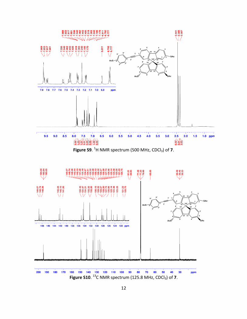
Figure S9. 1H NMR spectrum (500 MHz, CDCl3) of 7.

Figure S10. 13C NMR spectrum (125.8 MHz, CDCl3) of 7.

2

34

11

101

12

13 9,9'

56

7

8 SAc

13'

12' 11'

10'

4'

3'

2'

1'8'

7'

6'

5' SAcAcS

1'

2'1''

6''5''

4''

3''2''

AcS

2

34

11

101

12

13 9,9'

56

7

8 SAc

13'

12' 11'

10'

4'

3'

2'

1'8'

7'

6'

5' SAcAcS

1'

2'1''

6''5''

4''

3''2''

AcS

12

Figure S11. 1H NMR spectrum (500 MHz, CDCl3) of 9.

Figure S12. 13C NMR spectrum (125.8 MHz, CDCl3) of 9.

7

65

12

138

11

10

9

43

2

1

CH3H3C

I Br

7

65

12

138

11

10

9

43

2

1

CH3H3C

I Br

13

Figure S13. 1H NMR spectrum (500 MHz, CDCl3) of 10.

Figure S14. 13C NMR spectrum (125.8 MHz, CDCl3) of 10.

7

65

12

138

11

10

9

43

2

1

CH3H3C

1' Br2'

1''

6''5''

4''

3''2''

S

TMS

7

65

12

138

11

10

9

43

2

1

CH3H3C

1' Br2'

1''

6''5''

4''

3''2''

S

TMS

14

Figure S15. 1H NMR spectrum (500 MHz, CDCl3) of 11.

Figure S16. 13C NMR spectrum (125.8 MHz, CDCl3) of 11.

7

65

12

138

11

10

9

43

2

1

CH3H3C

1'S2'

1''

6''5''

4''

3''2''

S

TMS

TMS

7

65

12

138

11

10

9

43

2

1

CH3H3C

1'S2'

1''

6''5''

4''

3''2''

S

TMS

TMS

15

Figure S17. 1H NMR spectrum (500 MHz, CDCl3) of 12.

Figure S18. 13C NMR spectrum (125.8 MHz, CDCl3) of 12.

7

65

12

138

11

10

9

43

2

1

CH3H3C

1' SAc2'1''

6''5''

4''

3''2''

AcS

7

65

12

138

11

10

9

43

2

1

CH3H3C

1' SAc2'1''

6''5''

4''

3''2''

AcS

16

2. Electrode distance calibration

The first step of molecular junction characterization is the determination of preferred conductance values. This can be done by repeatedly opening and closing the junction. If a molecular junction is formed, the conductance-distance curves may show a series of steps and plateaus while the electrodes are separated with a constant velocity. The plateau values and lengths are characteristic for the metal-molecule combination under study.

The breaking mechanics is controlled by a DC motor with position sensor (Faulhaber, model 22/2, reduction ratio 1:1734) connected with a vacuum feedthrough into the cryostat that drives a rotary axis, see Fig. S19. The rotation of the axis is transformed into a lateral motion of a pushing rod by using a differential screw. The conductance is recorded by an automatic variable-gain source-meter (Keithley, model 6430), as shown in the schematic view of the setup in Fig. S20.

Technically, the conductance is measured as a function of the motor position. The motor position is then translated into an axial motion of the pushing rod.

Figure S19. (a) Sketch of the MCBJ mechanics consisting of pushing rod and two counter supports. (b) Realization of the mechanics using a diff-erential screw connected to a rotary axis. The differ-ential screw moves the counter supports upward and downward thereby bending the sample.

The interelectrode distance change (Δs) is estimated from the displacement of the pushing rod (Δz) via an attenuation factor (r):

∆𝑠𝑠 = 𝑟𝑟∆𝑧𝑧 (S1)

where

𝑟𝑟 = 𝜉𝜉 6𝑡𝑡𝑡𝑡𝐿𝐿2

(S2).

Here, t ≈ 0.25 mm is the thickness of the substrate, u ≈ 2 μm is the length of the free-standing bridge, L = 16 mm is the distance of the counter supports, and ξ is a correction factor which has a value varying from 2 to 4 depending on details of the sample.S5 r can be determined experimentally from conductance-distance curves in the tunnelling regime, when the work function of the electrode is known. By using the value Φ0 = 5.1 eV for Au, we estimate ξ = 4 for

17

our samples. However, since the distance u varies from sample to sample as well, the distance values bear an uncertainty of roughly 50%.

3. Electrical circuit

Figure S20. Schematics of the experimental setup for investigating the electronic properties of molecular junctions. List of abbreviations: LIA: Lock-In Amplifier, DMM: Digital MultiMeter, SMA: SubMiniature coaxial cable connectors, PC: Personal Computer, GPIB: General Purpose Interface Bus

4. Vibrational mode assignment

Table S1 shows a comparison between IET measurements and calculations.

Modes Description Theory Experiment LOP (Au-Au) Au-Au longitudinal

optical phonon 0.01-0.02 eV 0.01-0.016 eV

ν (Au-S) Au-S stretching 0.037 eV, 0.046 eV 0.038-0.044 eV ν (C-S) C-S stretching 0.052 eV, 0.075 eV 0.054-0.068 eV

γOP (C-H) C-H out of plane bending

0.094-0.11 eV 0.097-0.108 eV

γIP (C-H) C-H in plane bending 0.12 eV, 0.16 eV 0.144-157 eV ν (C=C) C=C stretching 0.18-0.2 eV 0.185-0.193 eV ν (C≡C) C≡C stretching 0.27 eV 0.274-0.283 eV ν (C-H) C-H stretching 0.3-0.38 eV 0.35 eV

Table S1. Summary of the vibrational mode assignment in the IET spectra for SBF molecular junctions. Peak positions in the spectra are identified by our theoretical IET calculations.

18

5. Control experiments

The control experiments were performed for two types of molecules. The first one is a monopodal molecule, displayed in Fig. S21(a), with the same backbone and length as the SBF. Fig. S21(b) and (c) show selected opening traces as well as a conductance histogram. The preferred conductance value of this backbone molecule is Gbackbone ≈ 10-3 G0, close to those of the SBF molecule. However, the trapping rate is only 8%, i.e. considerably lower than those for SBF, where the trapping rate amounts to 20%, as revealed by the rather small height of the maximum compared to the weight of the single-atom contacts with conductances around 1 G0. The plateau length is roughly a factor of 2 larger than those of the last plateaus of the gold contacts, in agreement with the molecule length of 1.7 nm and the fact that gold forms chains with up to 7 atoms in length.S6

The second control molecule features a cyano end group at the arm instead of a thiol, as shown in Fig. S22(a). Conductance-distance traces and the related conductance histogram are presented in Fig. S22(b) and (c). For this molecule the trapping rate is 12%, and we find a broad distribution of conductance values between 10-6 and 1 G0. This finding indicates that the molecules do not favor a particular robust junction geometry, presumably due to the weak physisorption of the cyano end group at low temperature. The weak maximum around 4·10-2 G0 is statistically not significant. The highly conductive junctions with G > 10-1 G0 may correspond to tunnelling between the Au electrodes, eventually through a barrier given by non-specifically absorbed molecules. These control experiments show that a robust binding geometry is necessary to provide well-defined conductance values and highly conductive molecular wires.

Figure S21. (a) Scheme of the monopodal molecule with the same backbone and length as SBF. (b) Conductance traces for SBF monopodal molecules. (c) Conductance histogram for the molecule shown in (a).

19

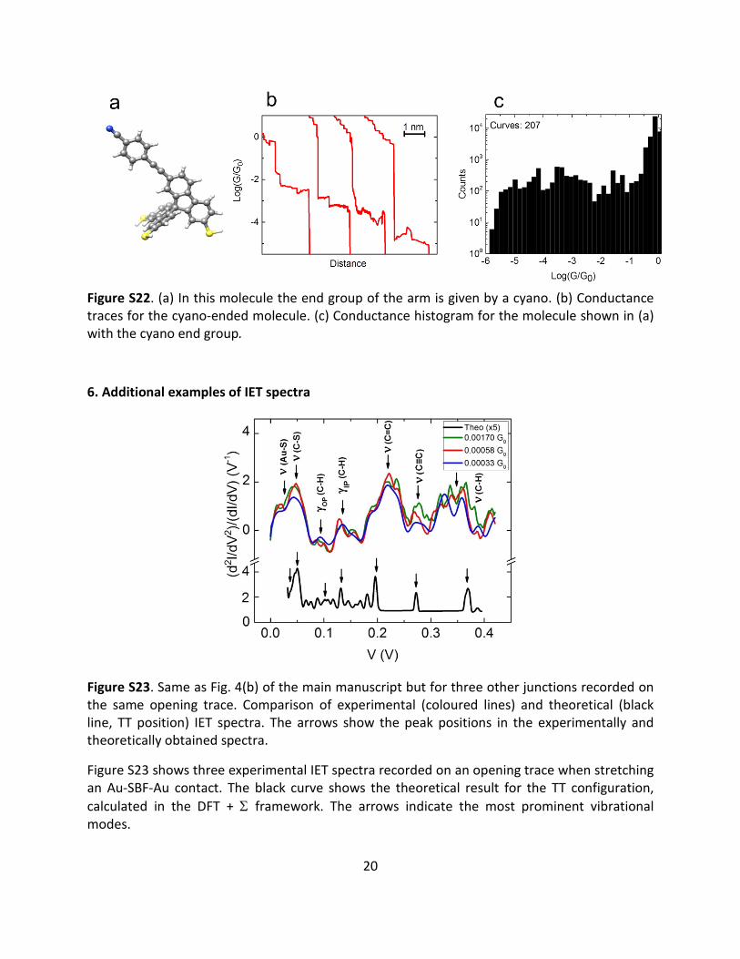
Figure S22. (a) In this molecule the end group of the arm is given by a cyano. (b) Conductance traces for the cyano-ended molecule. (c) Conductance histogram for the molecule shown in (a) with the cyano end group.

6. Additional examples of IET spectra

Figure S23. Same as Fig. 4(b) of the main manuscript but for three other junctions recorded on the same opening trace. Comparison of experimental (coloured lines) and theoretical (black line, TT position) IET spectra. The arrows show the peak positions in the experimentally and theoretically obtained spectra.

Figure S23 shows three experimental IET spectra recorded on an opening trace when stretching an Au-SBF-Au contact. The black curve shows the theoretical result for the TT configuration, calculated in the DFT + Σ framework. The arrows indicate the most prominent vibrational modes.

20

7. Theory

7.1 Electronic structure calculations

The theoretical investigation of the quantum transport properties of complex molecules like SBF remains challenging because of the large number of atoms and the infinite, nonperiodic geometry of the system. DFT is one of the few operative ab-initio electronic structure methods which can handle the hybrid metal-molecule-metal contacts. On the other hand, due to self-interaction errors in the standard exchange-correlation functional and missing image charge effects, DFT-based methods have difficulties to accurately describe the energy gap and level alignment of molecules on metal surfaces. This can be improved by adding a self-energy correction, resulting in the DFT+Σ method.S7 The main difference between DFT and DFT+Σ results for a given contact geometry is typically a pronounced increase of the HOMO-LUMO gap by several eV in DFT+Σ as compared to DFT that arises from a decrease of the HOMO and increase of the LUMO energies. DFT+Ʃ results often show a good agreement with the experimental results for the conductance.S7,S8 Details regarding our method can be found in Ref. S9.

In Fig. S24 we present the DFT calculations for the transmission of the SBF molecule, the SBF’ configuration where the tip couples to the top of the spirobifluorene foot, and the backbone in HH, TT, and TT' configurations. They exhibit a HOMO-related resonance close to the Fermi energy and we compute conductance values of GDFT_SBF = 0.0076G0, GDFT_SBF’ = 0.005 G0, GDFT_HH = 0.018 G0, GDFT_TT = 0.52 G0 and GDFT_TT’ = 0.67 G0. We assume that the unrealistically high conductance values of the DFT calculations are an artefact of the level-alignment problem and underestimation of the HOMO-LUMO gap common to DFT. Also the spread of the conductance values is much higher than in the DFT+Σ calculations, presented in the main text. For the TT configuration also in the DFT framework a pronounced shoulder develops around EF+1.3 eV, in agreement with the findings for DFT+Σ.

In Figure S25 we compare the DFT+Σ results for the transmissions of SBF and SBF’ as well as their IET spectra. The conductance of SBF’ is GSBF’ = 0.0039 G0, which is a factor of 4 larger than what we calculate for SFB in the configuration displayed in Fig. S25(a). The IET spectrum reveals that the C-C triple bond stretching mode is shifted to 252 mV. Its peak shows a factor of three smaller amplitude than those found for SBF.

21

Figure S24. (a) SBF (tripod) molecule on an Au(111) surface. (b) SBF molecule when one electrode couples to the middle of the molecule, called SBF’. Backbone molecule in (c) hollow-hollow (HH) and (d) top-top (TT) configurations. (e) The stretched molecule in TT (TT’) position. (e) Computed transmission curves for the SBF, SBF’, HH, TT, and TT' configurations in the DFT framework.

Figure S25. (a) SBF molecule on an Au(111) surface. (b) SBF’ configuration of SBF, when one electrode couples to the middle of the molecule. DFT+ Σ results for SBF and SBF’: (c) Transmissions as a function of energy, (d) IET spectra. The data for SBF are the same as discussed in the main text (see Figs. 2 and 5).

22

7.2 Landauer approach and single-level model

In the Landauer approach the stationary current is given by

𝐼𝐼 = 2𝑒𝑒ℎ ∫ 𝑑𝑑𝑑𝑑 𝜏𝜏(𝑑𝑑)(𝑓𝑓(𝑑𝑑 − 𝜇𝜇𝐿𝐿) − 𝑓𝑓(𝑑𝑑 − 𝜇𝜇𝑅𝑅)∞

−∞ , (S3)

where 𝜏𝜏(𝑑𝑑) = 4Tr[Γ𝐿𝐿𝐺𝐺𝐶𝐶𝑟𝑟Γ𝑅𝑅𝐺𝐺𝐶𝐶𝑎𝑎] can be calculated from Green’s functions and DFT input of the electronic structure.S10 For the linear conductance one obtains

𝐺𝐺 = 𝑑𝑑𝑑𝑑𝑑𝑑𝑑𝑑�𝑑𝑑=0

= 2𝑒𝑒2

ℎ ∫ 𝑑𝑑𝑑𝑑(−𝜕𝜕𝐸𝐸𝑓𝑓) 𝜏𝜏(𝑑𝑑)∞−∞ . (S4)

The experimental current-voltage characteristics are evaluated using the single-level model. This model assumes a single molecular orbital at energy E0 coupled to each lead via the coupling constants Γ𝐿𝐿 and Γ𝑅𝑅. This yields a resonance with Lorentzian shape for the transmission:

𝜏𝜏(𝑑𝑑) = 4Γ𝐿𝐿Γ𝑅𝑅(𝐸𝐸−𝐸𝐸0)2+(Γ𝐿𝐿+Γ𝑅𝑅)2

. (S5)

The current is calculated as integration over the bias window using the Landauer formula Eq. (S3). From the fitting procedure we obtain the values for the energy level (E0) and the level broadening (Γ = Γ𝐿𝐿 + Γ𝑅𝑅) that are displayed in Fig. 3(b) and (c) of the main text. If the molecule is symmetrically coupled to both electrodes, the two coupling constants are the same (Γ 2� = Γ𝐿𝐿 = Γ𝑅𝑅). Consequently, the I-V is (anti)symmetric (I(V) = -I(-V)). A molecule displays a rectifying behaviour for asymmetric couplings.S11-S14

7.3 AC broadening

Several vibrational modes can be hidden in one peak of an IET spectrum due to the AC broadening, as shown in Fig. S26 for the Au-S and C-S stretching modes.

Figure S26. Theoretical IET spectra for several AC voltages (3, 5, 7 and 9 mV) show how the related broadening leads to the overlapping of mode-related peaks, in particular of the Au-S and C-S vibrational modes. The spectra for 5, 7 and 9 mV are offset for clarity.

7.4 Lorentzian fit Our energy-dependent transmission curves in Fig. 2 of the main text show that the conductance of the SBF-based junctions is largely dominated by a single level, the HOMO. For this reason the single-level model is applicable, and to compare to the experiments we extract the level

23

alignment E0 and the coupling strengths ΓL and ΓR by fitting Lorentzians (see Eq. (S5)) to the HOMO-peaks of the transmission curves calculated in the DFT+Σ framework. Since left and right coupling strengths cannot be distinguished, we choose ΓL ≤ ΓR. Figure S27 shows the quality of the fit by comparing the original and fitted theoretical transmission curves.

DFT+Ʃ ГL (eV) ГR (eV) E0 (eV)

SBF 0.010 0.048 1.20 HH 0.023 0.027 1.57 TT 0.014 0.017 0.76 TT’ 0.009 0.010 0.95

Table S2. Single-level model parameters extracted from a Lorentzian fit to the transmission curves shown in Fig. 2 of the main text for SBF, HH, TT and TT’ configurations. The HOMO resonance is fitted with the single-level model of Eq. (S5), see Fig. S27.

The values presented in Fig. 3 of the main text range between 0.5 eV ≤ E0 ≤ 1 eV and 0.004 eV ≤ ΓL, ΓR ≤ 0.024 eV. The theoretical values that we list in Table S2 are in reasonable agreement. In detail, our theoretically estimated level alignment of 0.76 eV ≤ E0 ≤ 1.57 eV is slightly shifted towards stronger off-resonance conditions, while the electronic couplings with 0.008 eV ≤ ΓL,ΓR ≤ 0.048 eV appear to be more accurately represented.

Figure S27. Computed trans-mission curves for (a) SBF, (b) HH, (c) TT, and (d) TT' configurations in the DFT+Σ framework and related fits within a single-level model that describes the HOMO resonance by a Lorentzian function.

24

REFERENCES

S1 C. J. Yu, Y. Chong, J. F. Kayyem and M. Gozin, J. Org. Chem. 1999, 64, 2070-2079.

S2 V. Kolivoška, M. Mohos, I. V. Pobelov, S. Rohrbach, K. Yoshida, W. Hong, Y. C. Fu, P. Moreno-García, G. Mészáros, P. Broekmann, M. Hromadová, R. Sokolová, M. Valášek and T. Wandlowski, Chem. Comm. 2014, 50, 11757-11759.

S3 M. Valášek, K. Edelmann, L. Gerhard, O. Fuhr, M. Lukas and M. Mayor, J. Org. Chem. 2014, 79, 7342-7357.

S4 Y.-H. Chan, J.-T. Lin, I.-W. P. Chen and C.-H. Chen, J. Phys. Chem. B 2005, 109, 19161-19168.

S5 S. A. G. Vrouwe, E. van der Giessen, S. J. van der Molen, D. Dulic, M. L. Trouwborst and B. J. van Wees, Phys. Rev. B 2005, 71, 035313.

S6 N. Agrait, A. Levy Yeyati and J. M. van Ruitenbeek, Phys. Rep. 2003, 377, 81-279.

S7 S. Y. Quek, L. Venkataraman, H. J. Choi, S. G. Louie, M. S. Hybertsen and J. B. Neaton, Nano Lett. 2007, 7, 3477-3482.

S8 D. J. Mowbray, G. Jones and K. S. Thygesen, J. Chem. Phys. 2008, 128, 111103.

S9 L. A. Zotti, M. Bürkle, F. Pauly, W. Lee, K. Kim, W. Jeong, Y. Asai, P. Reddy and J. C. Cuevas, New J. Phys. 2014, 16, 015004.

S10 F. Pauly, J. K. Viljas, U. Huniar, M. Häfner, S. Wohlthat, M. Bürkle, J. C. Cuevas and G. Schön, New J. Phys. 2008, 10, 125019.

S11 A. S. Martin, J. R. Sambles and G. J. Ashwell, Phys. Rev. Lett. 1993, 70, 218-221.

S12 S. Parashar, P. Srivastava, M. Pattanaik and S. K. Jain, Eur. Phys. J. B 2014, 87, 220.

S13 K. Wang, J. Hamill, J. Zhou, C. Guo and B. Xu, Faraday Discuss. 2014, 174, 91-104.

S14 H. Liu, Y. He , J. Zhang, J. Zhao and L. Chen, Phys. Chem. Chem. Phys. 2015, 17, 4558-4568.

25