supplementary information for - rsc.org · 1 supplementary information for early stages of insulin...
TRANSCRIPT

1
Supplementary Information for
Early stages of insulin fibrillogenesis examined with
ion mobility mass spectrometry and molecular
modelling
Authors:
Harriet Cole#†, Massimiliano Porrini†, Ryan Morris†, Tom Smith#, Jason
Kalapothakis#†, Stefan Weidt#, C. Logan Mackay#, Cait E. MacPhee† & Perdita E.
Barran*1
Author Affiliations
#EastChem School of Chemistry, Joseph Black Building, The King’s Buildings,
West Mains Rd, Edinburgh EH9 3JJ
† SUPA, School of Physics and Astronomy, James Clark Maxwell Building, The
King’s Buildings, West Mains Rd, Edinburgh EH9 3JZ
*Michael Barber Centre for Collaborative Mass Spectrometry, School of
Chemistry, Manchester Institute of Mass Spectrometry, The University of
Manchester, Manchester, M1 7DN
Electronic Supplementary Material (ESI) for Analyst.This journal is © The Royal Society of Chemistry 2015

2
Supplementary Information ........................................................................................... 1 1. Supplementary MS and IM-MS data ..................................................................... 3
1.1 Cone Voltage Experiments .......................................................................... 3 1.2 Concentration Experiments ......................................................................... 5
1.3 Injection Energy Studies .............................................................................. 6 ATD, FTICR MS and CID data ............................................................................. 8
2. Supplementary Structural Characterisation ............................................................. 15 2.1 Collision Cross Sectional Values ................................................................... 15 2. 2 Graph of CCSs .............................................................................................. 17
2.4 Number of Charges on Protein Surface ......................................................... 18 3. Experimental Methodology ..................................................................................... 18
3.1 Fitting of ATD peaks ..................................................................................... 19 3.2 Source Conditions .......................................................................................... 21 3.3 Thioflavin T binding assay ............................................................................ 21 3.4 Transmission Electron Microscopy ............................................................... 22
4. Simulation Methodology ......................................................................................... 22
4.1 Molecular Modelling ......................................................................................... 22 4.2 Monomeric species [M+3H]3+ and [M+4H]4+ ................................................... 22
4.3 Correlation between CCS and Rg ....................................................................... 23 4.4 Contact interface and stability of dimers derived from docking ........................ 24
4.4.1 Breakdown of the contributions to the binding energy of representative
dimers ................................................................................................................... 25 4.4.2 CCSs of dimer structures from dynamics in water solvent......................... 26
5. References ................................................................................................................ 26

3
1. Supplementary MS and IM-MS data
1.1 Cone Voltage Experiments
Mass spectra of insulin were taken at different cone voltages. When the cone voltage is
increased; aggregate species are observed to break up.
1000 1500 2000 2500 3000
cone voltage:
100V
90V
70V
50V
30V
10V
[M+
4H
]4+
[M+
3H
]3+
[M+
5H
]5+
[M+
6H
]6+
[2M
+7H
]7+
[4M
+11H
]11
+
[3M
+8H
]8+
[2M
+5H
]5+
[3M
+7H
]7+
[5M
+11H
]11
+
[2M
+4H
]4+
m/z
1000 1500 2000 2500 3000
cone voltage:
100V
90V
70V
50V
30V
10V
[M+
4H
]4+
[M+
3H
]3+
[M+
5H
]5+
[M+
6H
]6+
[2M
+7H
]7+
[4M
+11H
]11
+
[3M
+8H
]8+
[2M
+5H
]5+
[3M
+7H
]7+
[5M
+11H
]11
+
[2M
+4H
]4+
m/z
Figure S1 | Spectra at increasing cone voltages between 10V and 100V showing
oligomer population changes.
4
cone voltage: 60V
55V
50V
40V
[M+
4H
]4+
[M+
3H
]3+
[M+
5H
]5+
[M+
6H
]6+
[2M
+7H
]7+
[4M
+11H
]11
+
[3M
+8H
]8+
[2M
+5H
]5+
[3M
+7H
]7+
[5M
+11H
]11
+
[2M
+4H
]4+
1000 1500 2000 2500 3000
1000 1500 2000 2500 3000
1000 1500 2000 2500 3000
1000 1500 2000 2500 3000
m/z
cone voltage: 60V
55V
50V
40V
[M+
4H
]4+
[M+
3H
]3+
[M+
5H
]5+
[M+
6H
]6+
[2M
+7H
]7+
[4M
+11H
]11
+
[3M
+8H
]8+
[2M
+5H
]5+
[3M
+7H
]7+
[5M
+11H
]11
+
[2M
+4H
]4+
1000 1500 2000 2500 3000
1000 1500 2000 2500 3000
1000 1500 2000 2500 3000
1000 1500 2000 2500 3000
m/z
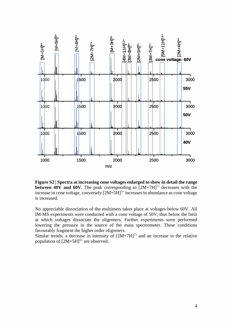
Figure S2 | Spectra at increasing cone voltages enlarged to show in detail the range
between 40V and 60V. The peak corresponding to [2M+7H]7+ decreases with the
increase in cone voltage, conversely [2M+5H]5+ increases in abundance as cone voltage
is increased.
No appreciable dissociation of the multimers takes place at voltages below 60V. All
IM-MS experiments were conducted with a cone voltage of 50V, thus below the limit
at which voltages dissociate the oligomers. Further experiments were performed
lowering the pressure in the source of the mass spectrometer. These conditions
favourably fragment the higher order oligomers.
Similar trends; a decrease in intensity of [2M+7H]7+ and an increase in the relative
population of [2M+5H]5+ are observed.
5
1.2 Concentration Experiments
10µM
100µM
200µM
500µM
1000µM
2500µM
[M+
6H
]6+
[M+
5H
]5+
[M+
4H
]4+
[M+
3H
]3+
[2M
+5H
]5+
1000 1200 1400 1600 1800 2000 2200 2400 2600 2800 3000
Inte
nsity / a
rbitra
ry u
nits
m/z
10µM
100µM
200µM
500µM
1000µM
2500µM
[M+
6H
]6+
[M+
5H
]5+
[M+
4H
]4+
[M+
3H
]3+
[2M
+5H
]5+
10µM
100µM
200µM
500µM
1000µM
2500µM
[M+
6H
]6+
[M+
5H
]5+
[M+
4H
]4+
[M+
3H
]3+
[2M
+5H
]5+
1000 1200 1400 1600 1800 2000 2200 2400 2600 2800 3000
Inte
nsity / a
rbitra
ry u
nits
m/z
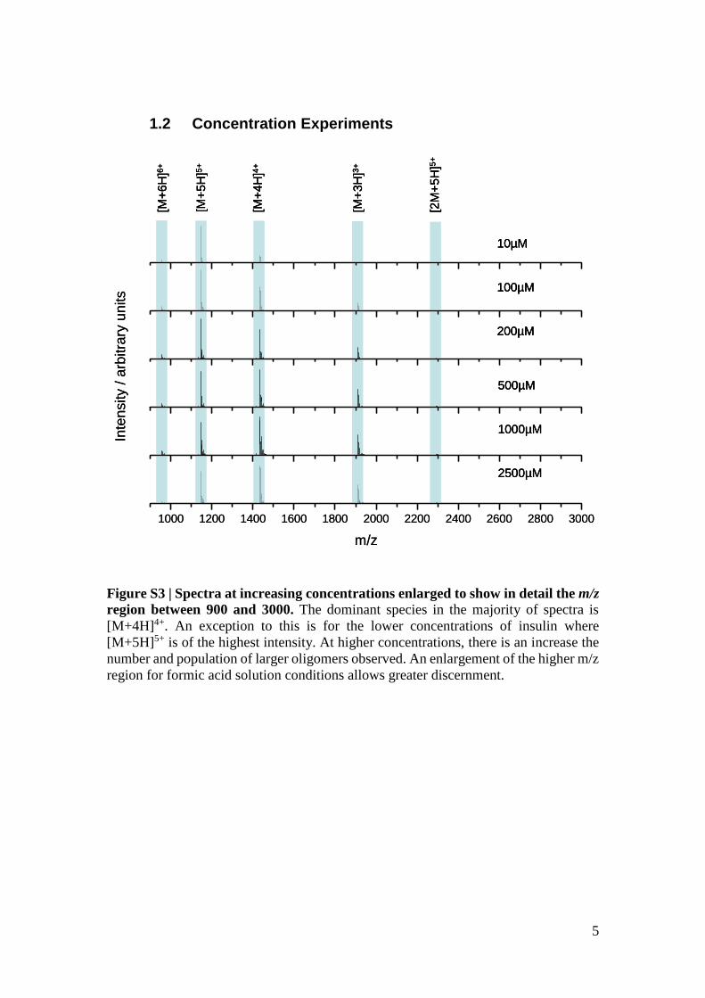
Figure S3 | Spectra at increasing concentrations enlarged to show in detail the m/z
region between 900 and 3000. The dominant species in the majority of spectra is
[M+4H]4+. An exception to this is for the lower concentrations of insulin where
[M+5H]5+ is of the highest intensity. At higher concentrations, there is an increase the
number and population of larger oligomers observed. An enlargement of the higher m/z
region for formic acid solution conditions allows greater discernment.

6
10µM
100µM
200µM
500µM
1000µM
2500µM
[5M
+9H
]9+
[4M
+7H
]7+
[6M
+10H
]10
+
[5M
+8H
]8+
[6M
+9H
]9+
[7M
+10H
]10
+
[7M
+11H
]11
+
[8M
+10H
]10
+
[7M
+12H
]12
+
[5M
+7H
]7+
[6M
+8H
]8+
3000 3200 3400 3600 3800 4000 4200 4400 4600 4800 5000
Inte
nsity / a
rbitra
ry u
nits
m/z
10µM
100µM
200µM
500µM
1000µM
2500µM
[5M
+9H
]9+
[4M
+7H
]7+
[6M
+10H
]10
+
[5M
+8H
]8+
[6M
+9H
]9+
[7M
+10H
]10
+
[7M
+11H
]11
+
[8M
+10H
]10
+
[7M
+12H
]12
+
[5M
+7H
]7+
[6M
+8H
]8+
3000 3200 3400 3600 3800 4000 4200 4400 4600 4800 5000
Inte
nsity / a
rbitra
ry u
nits
m/z
Figure S4 | Spectra at increasing insulin concentration enlarged to show in detail
the m/z region between 3000 and 5000. At 500μM and above a wide range of larger
oligomers are present at significant intensities. Higher order oligomer populations
remain quantitatively similar with increasing concentrations after a threshold of 500μM
has been reached. A solution of aqueous formic acid containing insulin at a
concentration of 523μM was chosen for the majority of further experiments.
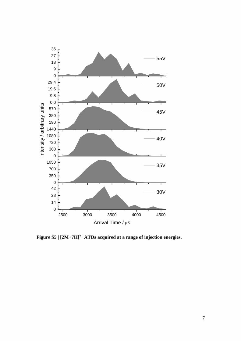
1.3 Injection Energy Studies
Injection energy studies were carried out to ensure that the extended oligomer
conformers observed were not caused by structural unfolding in the gas phase due to
activation of the ions by high-energy collisions as they are transported in the mass
spectrometer. IM-MS data was acquired whilst varying the voltage that injects the ions
into the drift tube, known as the injection energy. An set of ATDs of the [2M+7H]7+
are shown below, as this is one of the oligomeric species which possesses extended
conformers.
7
2500 3000 3500 4000 4500
0
14
28
42
0
350
700
1050
0
360
720
1080
14400
190
380
570
0.0
9.8
19.6
29.4
0
9
18
27
36
Arrival Time / s
30V
35V
Inte
nsity / a
rbitra
ry u
nits
40V
45V
50V
55V
Figure S5 | [2M+7H]7+ ATDs acquired at a range of injection energies.

8
1.4 Acidifying with HCl
a
b

9
Figure S6 | A TEM image of 4mg/ml insulin solution, incubated over 3 days at 60°C
in solutions acidified with HCl
B nESI Mass Spectra at increasing insulin concentration when it has been
acidified with HCl . At 500μM and above a wide range of larger oligomers are
present at significant intensities. The insert shows the extent of aductation due to
chloride species.
10
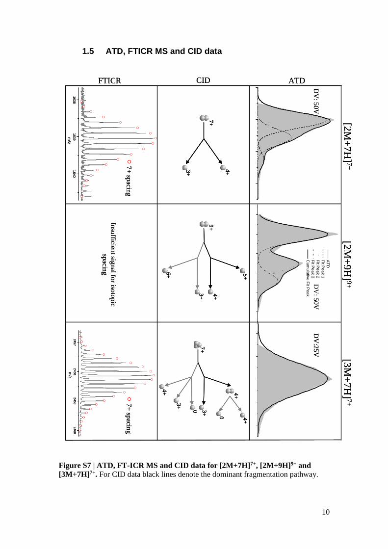
1.5 ATD, FTICR MS and CID data
Figure S7 | ATD, FT-ICR MS and CID data for [2M+7H]7+, [2M+9H]9+ and
[3M+7H]7+. For CID data black lines denote the dominant fragmentation pathway.
1638
1639
1640
m/z
2457
2458
2459
2460
m/z
CIDFTICR
[2M
+7
H]7+
Insu
fficient sig
nal fo
r isoto
pic
spacin
g
[2M
+9
H]9+
[3M
+7
H]7+
4+3+
7+
4+
3+
7+
4+
0
0
3+
4+
9+
3+
6+ 5+
4+
AT
D
Fit P
ea
k 1
Fit P
ea
k 2
Fit P
ea
k 3
Cu
mu
lativ
e F
it Pe
ak
ATD
7+
spacin
g7+
spacin
g
DV
: 50V
DV
: 50V
DV
:25V
1638
1639
1640
m/z
2457
2458
2459
2460
m/z
CIDFTICR
[2M
+7
H]7+
Insu
fficient sig
nal fo
r isoto
pic
spacin
g
[2M
+9
H]9+
[3M
+7
H]7+
4+3+
7+
4+3+
7+
4+3+
7+
4+
3+
7+
4+
0
0
3+
4+ 4
+
3+
7+
4+
0
0
3+
4+
9+
3+
6+ 5+
4+
9+
3+
6+ 5+
4+
AT
D
Fit P
ea
k 1
Fit P
ea
k 2
Fit P
ea
k 3
Cu
mu
lativ
e F
it Pe
ak
ATD
7+
spacin
g7+
spacin
g
DV
: 50V
DV
: 50V
DV
:25V

11
Figure S8 | ATD, FT-ICR MS and CID data for [3M+8H]8+, [4M+9H]9+ and
2085
2086
2087
m/z
2150
2151
2152
m/z
CIDFTICR
[3M
+8H
]8+
4+
5+
8+
3+
4+ A
TD
Fit P
ea
k 1
Fit P
ea
k 2
Fit P
ea
k 3
Cu
mu
lativ
e F
it Pe
ak
ATD
2548
2549
2550
2551
m/z
[4M
+9H
]9+
3+
9+
6+
[4M
+11H
]11+
11
+
3+
7+
4+
6+
5+
8+
2+
9+
AT
D
Fit P
ea
k 1
Fit P
ea
k 2
Fit P
ea
k 3
Fit P
ea
k 4
Cu
mu
lativ
e F
it Pe
ak
11+
spacin
g9+
spacin
g8+
spacin
g
DV
: 35V
DV
: 30V
DV
: 30V
2085
2086
2087
m/z
2150
2151
2152
m/z
CIDFTICR
[3M
+8H
]8+
4+
5+
8+
3+
4+
4+
5+
8+
3+
4+
8+
3+
4+ A
TD
Fit P
ea
k 1
Fit P
ea
k 2
Fit P
ea
k 3
Cu
mu
lativ
e F
it Pe
ak
ATD
2548
2549
2550
2551
m/z
[4M
+9H
]9+
3+
9+
6+
3+
9+
6+
3+
9+
6+
[4M
+11H
]11+
11
+
3+
7+
4+
6+
5+
8+
2+
9+
AT
D
Fit P
ea
k 1
Fit P
ea
k 2
Fit P
ea
k 3
Fit P
ea
k 4
Cu
mu
lativ
e F
it Pe
ak
11+
spacin
g9+
spacin
g8+
spacin
g
DV
: 35V
DV
: 30V
DV
: 30V

12
[4M+11H]11+. For CID data black lines denote the dominant fragmentation pathway.
Figure S9 | ATD, FTICR MS and CID data for [5M+11H]11+, [5M+12H]12+ and
[6M+11H]11+. For CID data black lines denote the dominant fragmentation pathway.
CIDFTICR ATD
[5M
+11H
]11+
11
+
3+
6+
5+
5+
8+
2+
4+
2606
2607
2608
m/z
[5M
+12H
]12+
12
+
3+
6+
8+
4+
4+
5+
6+
2389
2390
2391
m/z
[6M
+11H
]11+
3128
3129
m/z
AT
D
Fit P
ea
k 1
Fit P
ea
k 2
Fit P
ea
k 3
Cu
mu
lativ
e F
it Pea
k
11+
spacin
g12+
spacin
g11+
spacin
g
AT
D
Fitte
d P
ea
k
Insu
fficient sig
nal fo
r CID
AT
D
Fit P
ea
k 1
Fit P
ea
k 2
Cu
mu
lativ
e F
it Pea
k
DV
: 50V
DV
: 25V
DV
: 25V
CIDFTICR ATD
[5M
+11H
]11+
11
+
3+
6+
5+
5+
8+
2+
4+
11
+
3+
6+
5+
5+
8+
2+
4+
2606
2607
2608
m/z
[5M
+12H
]12+
12
+
3+
6+
8+
4+
4+
5+
6+
12
+
3+
6+
8+
4+
4+
5+
6+
2389
2390
2391
m/z
[6M
+11H
]11+
3128
3129
m/z
AT
D
Fit P
ea
k 1
Fit P
ea
k 2
Fit P
ea
k 3
Cu
mu
lativ
e F
it Pea
k
11+
spacin
g12+
spacin
g11+
spacin
g
AT
D
Fitte
d P
ea
k
Insu
fficient sig
nal fo
r CID
AT
D
Fit P
ea
k 1
Fit P
ea
k 2
Cu
mu
lativ
e F
it Pea
k
DV
: 50V
DV
: 25V
DV
: 25V
13
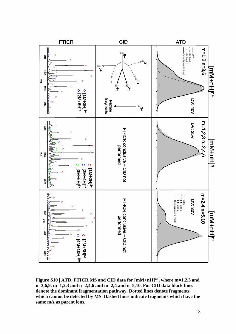
Figure S10 | ATD, FTICR MS and CID data for [mM+nH]n+, where m=1,2,3 and
n=3,6,9, m=1,2,3 and n=2,4,6 and m=2,4 and n=5,10. For CID data black lines
denote the dominant fragmentation pathway. Dotted lines denote fragments
which cannot be detected by MS. Dashed lines indicate fragments which have the
same m/z as parent ions.
AT
D
Fit P
ea
k 1
Fit P
ea
k 2
Cu
mu
lativ
e F
it Pea
k
AT
D
Fit P
ea
k 1
Fit P
ea
k 2
Cu
mu
lativ
e F
it Pea
k
CIDFTICR ATD
1911
1912
1913
1914
m/z
[2M
+6
H] 6
+
[1M
+3
H] 3
+
[mM
+n
H] n
+
2866
2868
2870
m/z
[3M
+6
H] 6
+
[2M
+4
H] 4
+
[1M
+2
H] 2
+
[mM
+n
H] n
+
m=
1,2
n=
3,6
m=
1,2
,3 n
=2,4
,6
[mM
+n
H] n
+
m=
2,4
n=
5,1
0
2294
2295
2296
m/z
[2M
+5
H] 5
+
[4M
+10
H] 1
0+
DV
: 25
VD
V: 3
0V
DV
: 40
V
3+
Pe
ptid
e
fragm
ents
5+
2+
4+
6+
+ 3+
3+
FT
-ICR
co
nclu
siv
e –
CID
no
t
pe
rform
ed
FT
-ICR
co
nclu
siv
e –
CID
no
t
pe
rform
ed
AT
D
Fit P
ea
k 1
Fit P
ea
k 2
Cu
mu
lativ
e F
it Pea
k
AT
D
Fit P
ea
k 1
Fit P
ea
k 2
Cu
mu
lativ
e F
it Pea
k
CIDFTICR ATD
1911
1912
1913
1914
m/z
[2M
+6
H] 6
+
[1M
+3
H] 3
+
[mM
+n
H] n
+
2866
2868
2870
m/z
[3M
+6
H] 6
+
[2M
+4
H] 4
+
[1M
+2
H] 2
+
[mM
+n
H] n
+
m=
1,2
n=
3,6
m=
1,2
,3 n
=2,4
,6
[mM
+n
H] n
+
m=
2,4
n=
5,1
0
2294
2295
2296
m/z
[2M
+5
H] 5
+
[4M
+10
H] 1
0+
DV
: 25
VD
V: 3
0V
DV
: 40
V
3+
Pe
ptid
e
fragm
ents
5+
2+
4+
6+
+ 3+
3+
AT
D
Fit P
ea
k 1
Fit P
ea
k 2
Cu
mu
lativ
e F
it Pea
k
AT
D
Fit P
ea
k 1
Fit P
ea
k 2
Cu
mu
lativ
e F
it Pea
k
CIDFTICR ATD
1911
1912
1913
1914
m/z
[2M
+6
H] 6
+
[1M
+3
H] 3
+
[mM
+n
H] n
+
2866
2868
2870
m/z
[3M
+6
H] 6
+
[2M
+4
H] 4
+
[1M
+2
H] 2
+
[mM
+n
H] n
+
m=
1,2
n=
3,6
m=
1,2
,3 n
=2,4
,6
[mM
+n
H] n
+
m=
2,4
n=
5,1
0
2294
2295
2296
m/z
[2M
+5
H] 5
+
[4M
+10
H] 1
0+
DV
: 25
VD
V: 3
0V
DV
: 40
V
3+
Pe
ptid
e
fragm
ents
5+
2+
4+
6+
+ 3+
3+
FT
-ICR
co
nclu
siv
e –
CID
no
t
pe
rform
ed
FT
-ICR
co
nclu
siv
e –
CID
no
t
pe
rform
ed

14
The [2M+7H]7+ ATDs are shifted to higher arrival times only when the injection
voltage is higher than 45V. All IM-MS experiments were performed with an injection
energy of 39.7V
Figure S11 Mass spectra taken at increasing collision energy showing the change
in the population of oligomers.

15
Figure S12 Zoom of data shown in Figure S11 to show in detail the m/z region
between 1500 and 2500. 2. Supplementary Structural Characterisation
2.1 Collision Cross Sectional Values
CCS / Ų
Species Average
Standard
Deviation
[M+6H]6+ 978.9 22.2
[M+5H]5+ 912.3 5.6
[M+4H]4+ 805.7 4.3
[M+3H]3+ 704.5 24.1
[2M+9H]9+ 1678.9 179.1
[2M+9H]9+ 2305.3 250.5
[2M+9H]9+ 2565.2 71.6
[2M+7H]7+ 1217.0 32.5
[2M+7H]7+ 1323.7 49.3
[2M+7H]7+ 1563.9 9.6
[2M+7H]7+ 1701.0 *
[2M+6H]6+ 1095.6 20.1

16
[2M+5H]5+ 1200.9 9.0
[2M+4H]4+ 961.3 17.0
[3M+10H]10+ 1609.2 333.0
[3M+10H]10+ 1722.9 35.4
[3M+10H]10+ 2560.9 136.6
[3M+8H]8+ 1621.9 97.7
[3M+8H]8+ 1764.3 48.1
[3M+8H]8+ 1948.3 *
[3M+7H]7+ 1682.1 14.6
[4M+11H]11+ 1954.2 47.9
[4M+11H]11+ 2363.6 107.3
[4M+11H]11+ 2731.0 7.2
[4M+11H]11+ 3034.8 *
[4M+10H]10+ 1907.1 84.5
[4M+ 9H]9+ 2160.4 102.6
[4M+7H]7+ 1754.2 40.7
[5M+12H]12+ 2249.5 49.6
[5M+12H]12+ 2622.0 4.7
[5M+12H]12+ 2911.3 107.5
[5M+12H]12+ 3418.7 *
[5M+11H]11+ 2259.4 64.3
[5M+11H]11+ 2516.9 30.5
[5M+11H]11+ 2877.9 *
[5M+9H]9+ 2265.7 35.0
[5M+8H]8+ 1982.8 57.4
[5M+7H]7+ 1680.3 8.3
[6M+13H]13+ 2207.9 148.5
[6M+13H]13+ 2663.4 108.7
[6M+13H]13+ 2997.8 80.2
[6M+13H]13+ 3246.5 *
[6M+13H]13+ 3673.1 *
[6M+11H]11+ 2695.9 86.1
[6M+10H]10+ 2465.2 41.2
[6M+9H]9+ 2205.2 26.2
[6M+8H]8+ 1888.6 62.3
[7M+13H]13+ 3113.1 64.7
[7M+12H]12+ 2938.0 66.6
[7M+11H]11+ 2791.2 68.2
[7M+10H]10+ 2399.6 82.6
[8M+15H]15+ 3608.7 102.6
[8M+13H]13+ 3198.7 60.7
[8M+11H]11+ 2575.3 63.6
[9M+14H]14+ 3476.1 29.5
[9M+13H]13+ 3146.3 62.0
[11M+17H]17+ 4134.9 46.7
[12M+17H]17+ 4040.2 36.3

17
Table ST1 | Rotationally averaged collision cross sections for all multimeric
species and conformations observed. The collision cross sections presented are the
average of three repeats with the associated standard deviation. * represents species
which were only identified in one repeat and therefore do not have an associated
standard deviation.
2. 2 Graph of CCSs
1 2 3 4 5 6 7 8 9 10 11 12
500
1000
1500
2000
2500
3000
3500
4000
4500
6543
65
4
7
10
9
7
9
8
7
11
10
9
8
131211
10
15
13
11
14
13
1717
77
77
9
9
9
8888
10
10
10
11
11
11
11
12
12
12
12
13
13
13
13
13
11
11
11
8
CC
S / Å
2
Multimeric Order / n
9 7
10 8
7
4
8
65
564
3
10
11
11 12
13
9 9
10
11
9
1 2 3 4 5 6 7 8 9 10 11 12
500
1000
1500
2000
2500
3000
3500
4000
4500
6543
65
4
7
10
9
7
9
8
7
11
10
9
8
131211
10
15
13
11
14
13
1717
77
77
9
9
9
8888
10
10
10
11
11
11
11
12
12
12
12
13
13
13
13
13
11
11
11
8
CC
S / Å
2
Multimeric Order / n
9 7
10 8
7
4
8
65
564
3
10
11
11 12
13
9 9
10
11
9
Figure S13 | Graph of multimeric order versus CCS for 523µM insulin in aqueous
pH2 formic acid. Labels are the associated charge state of each oligomer. Error bars
represent standard deviations of three repeated measurements.

18
2.4 Number of Charges on Protein Surface
A large number of charges will increase the CCS of an aggregate due to coulombic
repulsion 1,2. From de la Mora’s empirical relation for the maximum number of charges
on the surface of a protein which has retained its native fold (see main text), the graph
below plots this against the experimentally observed charge states for different
oligomeric orders. All of the observed species carry more charges than the multimeric
order of the oligomer.
1 2 3 4 5 6 7 8 9 10 11 12
2
3
4
5
6
7
8
9
10
11
12
13
14
15
16
17
18
19
20
21
experimentally observed
Ch
arg
e / +
ze
Multimeric Order
RMz 0778.0
Figure S14 | de la Mora relation The observed charge carried by each oligomer
compared to the de la Mora relation for the maximum number of charges able to be
carried on the surface of a protein which has retained its native fold.
The observed charge on all oligomeric species is consistent with the surface protonation
of a compact globular species, with exceptions [M+6H]6+ and [2M+9H]9+. Therefore
differences in the charge oligomers carry can be attributed to inherent structural
variations present in solution and not charge driven coulombic unfolding. A comparison
between the experimentally determined CCSs of insulin oligomers and those of other
globular proteins of comparable mass further supports this as they are very similar. A
similar argument has been put forward by Smith et al. 3.
3. Experimental Methodology

19
3.1 Fitting of ATD peaks
From the experimental ATDs the presence of multiple species coincident in m/z space
can be conferred. Additional information can be obtained by comparing the
experimentally determined ATDs with those predicted from models of ion transport.
Moseley et al. 4 have shown that the axial ion current J(x, t) generated from an infinitely
thin disk of ions drifting with constant velocity and diffusing in a drift tube is given by:
tD
r
L
tD
vtx
T
L
et
xv
tD
aetxJ
44
20
2
14
),(
Equation S2
where t is the drift time, x is the drift length, r0 the radius of the entrance aperture, v the
drift velocity, DL and DT the longitudal and transverse diffusion coefficients,
respectively and a a scaling factor which depends on the initial amount of ions and also
their transmission efficiency through the instrument. Two parameters in this expression
are of particular significance: the drift velocity and the longitudal diffusion coefficient.
The drift velocity is given by
KEv Equation. S3
K being the ionic mobility. At low field strength the diffusion coefficient and the
mobility are related via the Nernst-Einstein-Townsend relation:
Tk
zeDK
B
Equation S4
Thus, at least in theory, longitudal diffusion coefficients and drift speeds can be fitted
to a single parameter. Nevertheless, in the data collected for insulin and insulin
multimer ions sprayed from acidified solutions this is seldom the case. The peaks in the
arrival time spectrum are consistently broader than predicted from the Nernst-Einstein-
Townsend relation. This fact is illustrated in Figure S9. A number of factors not taken
into account with this model can contribute to the observed widening of the ATD. The
input pulse width is one example; nevertheless that alone cannot explain the observed
widths since the initial pulse cannot be spread over an interval greater than 40µs;
however ATD widths observed are of the order of milliseconds; therefore a difference
greater than 5% cannot be due to the initial pulse width. Another factor that is very
difficult to account for is the distortion of the longtitudinal ion distribution in regions
of the instrument outside the drift tube; since the ions pass through focusing ion optics
and a quadrupole mass analyzer, space-charge effects may also play a role. It can be
inferred from the experiments that ions spend several hundred of microseconds
(typically around 500 to 900µs) between the gate and the time of flight mass analyzer.
Yet, most interestingly, protein and protein aggregate ions may possess some
conformational heterogeneity, which will in turn give rise to broader peaks. Given the
low resolution of our ion mobility device ( tt lying between 3 and 5) it is very likely
that several distinct species remain unresolved. Thus, in the case of the [M+4H]4+
species (Figure S15a) we may infer the presence of significant conformational
variability in addition giving rise to a longtitudal diffusion coefficient that is on average
20
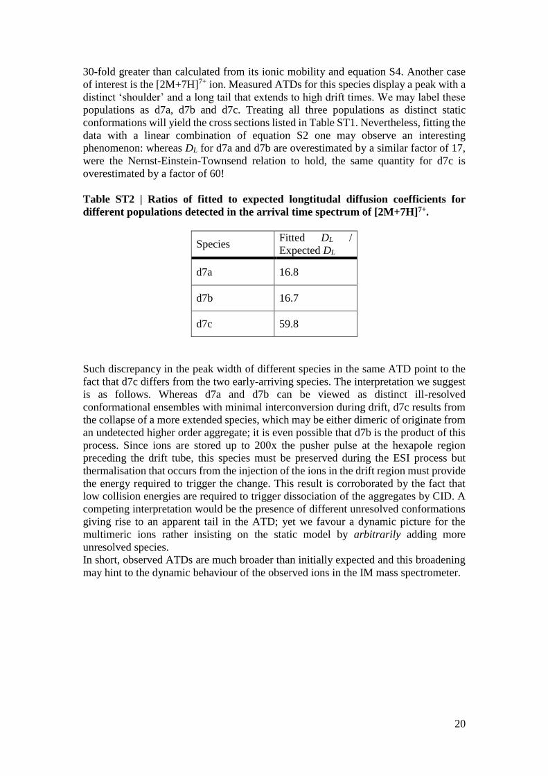
30-fold greater than calculated from its ionic mobility and equation S4. Another case
of interest is the [2M+7H]7+ ion. Measured ATDs for this species display a peak with a
distinct ‘shoulder’ and a long tail that extends to high drift times. We may label these
populations as d7a, d7b and d7c. Treating all three populations as distinct static
conformations will yield the cross sections listed in Table ST1. Nevertheless, fitting the
data with a linear combination of equation S2 one may observe an interesting
phenomenon: whereas DL for d7a and d7b are overestimated by a similar factor of 17,
were the Nernst-Einstein-Townsend relation to hold, the same quantity for d7c is
overestimated by a factor of 60!
Table ST2 | Ratios of fitted to expected longtitudal diffusion coefficients for
different populations detected in the arrival time spectrum of [2M+7H]7+.
Species Fitted DL /
Expected DL
d7a 16.8
d7b 16.7
d7c 59.8
Such discrepancy in the peak width of different species in the same ATD point to the
fact that d7c differs from the two early-arriving species. The interpretation we suggest
is as follows. Whereas d7a and d7b can be viewed as distinct ill-resolved
conformational ensembles with minimal interconversion during drift, d7c results from
the collapse of a more extended species, which may be either dimeric of originate from
an undetected higher order aggregate; it is even possible that d7b is the product of this
process. Since ions are stored up to 200x the pusher pulse at the hexapole region
preceding the drift tube, this species must be preserved during the ESI process but
thermalisation that occurs from the injection of the ions in the drift region must provide
the energy required to trigger the change. This result is corroborated by the fact that
low collision energies are required to trigger dissociation of the aggregates by CID. A
competing interpretation would be the presence of different unresolved conformations
giving rise to an apparent tail in the ATD; yet we favour a dynamic picture for the
multimeric ions rather insisting on the static model by arbitrarily adding more
unresolved species.
In short, observed ATDs are much broader than initially expected and this broadening
may hint to the dynamic behaviour of the observed ions in the IM mass spectrometer.

21
Figure S15 | Arrival time distributions for A) [M+4H]4+ and B) [2M+7H]7+ ions.
Black dots: experimental arrival time spectra; grey curves: ATDs fitted with equation
S1; black dotted curves: ATDs calculated with the same expression but by forcing DL
to comply with equation S3. Clearly experimental ATDs are broader than expected
from the aforementioned equation. A and B are not in scale.
3.2 Source Conditions
All instruments utilised n-ESI sources. The n-ESI source enables the production of ions
by charging solutions via the insertion of a thin platinum wire into capillary tips. This
produces a Taylor cone plume of ionised droplets which are guided into the mass
spectrometer down a voltage gradient. n-ESI capillaries were prepared from glass
capillaries (World Precision Instruments, Sarasota, USA) using a micropipette puller
(Fleming/Brown P-97 Sutter Instruments, Novato, USA).
For QTOF instruments (QTOF 2 and QTOF Ultima, (Waters, UK)) used an elevated
source pressure was used to reduce fragmentation of larger oligomeric species 5. The
source voltages were kept as low as possible to prevent fragmentation of oligomers,
whilst preserving sufficient signal intensity. QTOFs were calibrated with NaI and the
data was processed using Mass Lynx Software 4.1 (Micromass UK).
3.3 Thioflavin T binding assay
1.5mg/ml insulin samples were freshly prepared as stated above (3.1), filtered (using a
0.2μm filter) and thioflavin T (Th T) was added to a final concentration of 20μM. The
A
B
d7a
d7b
d7c

22
change in Th T fluorescence (excitation wavelength: 440nm, emission wavelength:
485nm) was monitored in a BMG Fluorostar optima plate reader, using clear
polystyrene 96-well plates coated with a PEG-like polymer (Corning 96-Well
Nonbinding Surface microplates). The plate was sealed and incubated at 60°C, the
fluorescence emission being recorded at 10-minute intervals. Thirty 100μL aliquots
were recorded on the same microplate (the average of all wells is shown in Figure 1 C
main text).
3.4 Transmission Electron Microscopy
Samples were stained for TEM took place in the following fashion, removing any
excess liquid after each step with a wedge of filter paper. 3μL of the sample of interest
were deposited onto a fomvar-coated copper grid (TAAB) and allowed to rest for 5
minutes. The grids were then washed with a droplet (ca. 10μL) of distilled water and
stained for 30-40seconds with 4 microlitres of 1% (m/v) uranyl acetate, before being
allowed to dry. TEM images were collected using a Philips CM 120 BioTwin
transmission electron microscope.
4. Simulation Methodology
4.1 Molecular Modelling
Table ST3 | CCS values for the multimeric species from monomer to hexamer. A
structure surface representation for all the species is given: the monomeric units closer
to the reader are depicted in orange, whilst the further away units are depicted in green.
4.2 Monomeric species [M+3H]3+ and [M+4H]4+
Since for a 51 residue protein, reproducing the aqueous medium through an explicit
solvent model would make unfolding and folding processes intractable from a
computational time point of view, the solvent was represented with a continuum
solvation method, termed “OBC” 6,7. The temperature control at 70◦C was effectuated
using the Langevin algorithm, with a collision frequency equal to 1.0 ps−1. All the bonds
involving hydrogen atoms were constrained at their equilibrium value using the
SHAKE algorithm 8, allowing the utilisation of a 2 fs time step.
Discarding the first 2ns (that is 1,000 structures) of the runs, with the remaining 75,000
ones a cluster analysis was performed 9. Specifically the bottom-up average-linkage
23
algorithm derived 10 clusters of conformations and implemented a sieve of 25. To
construct the similarity matrix of distances the backbone RMSD between the pairs of
structures was measured. This procedure resulted in 10 conformational families.
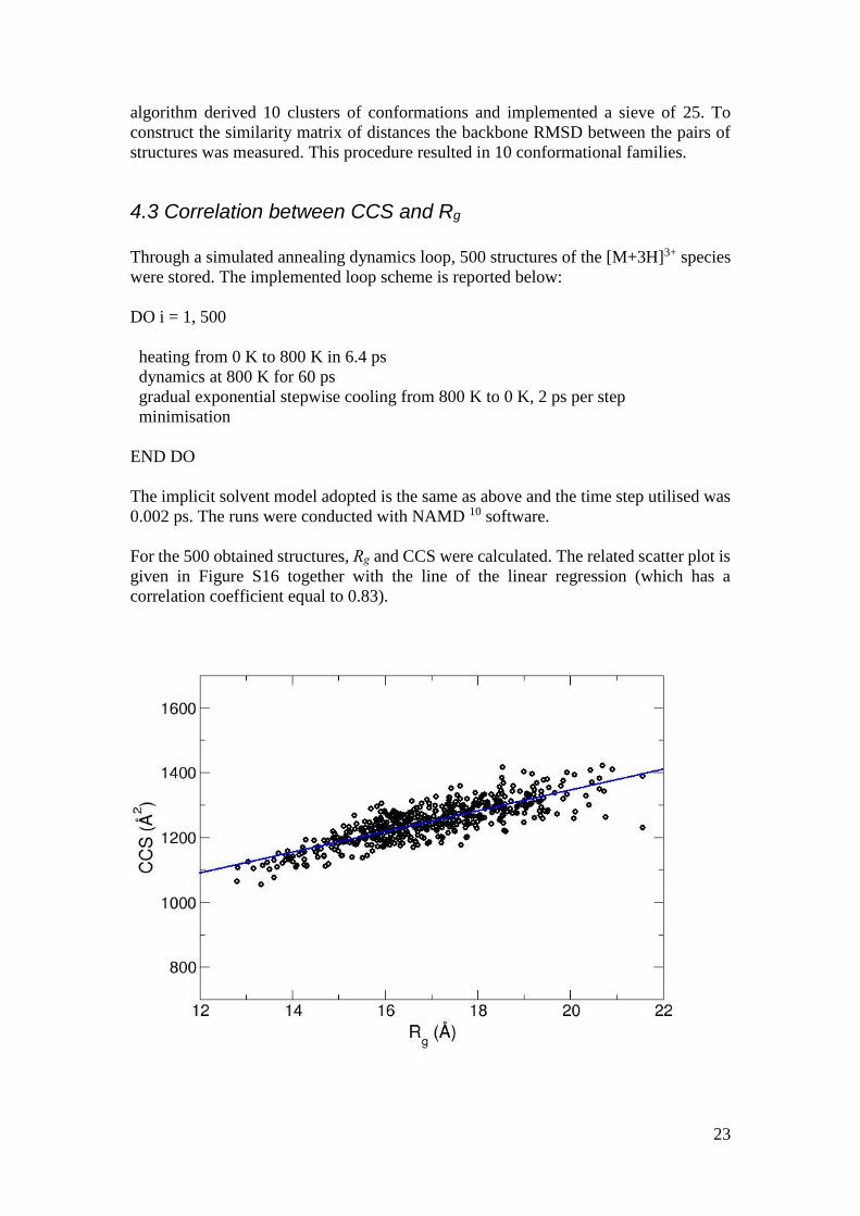
4.3 Correlation between CCS and Rg
Through a simulated annealing dynamics loop, 500 structures of the [M+3H]3+ species
were stored. The implemented loop scheme is reported below:
DO i = 1, 500
heating from 0 K to 800 K in 6.4 ps
dynamics at 800 K for 60 ps
gradual exponential stepwise cooling from 800 K to 0 K, 2 ps per step
minimisation
END DO
The implicit solvent model adopted is the same as above and the time step utilised was
0.002 ps. The runs were conducted with NAMD 10 software.
For the 500 obtained structures, Rg and CCS were calculated. The related scatter plot is
given in Figure S16 together with the line of the linear regression (which has a
correlation coefficient equal to 0.83).
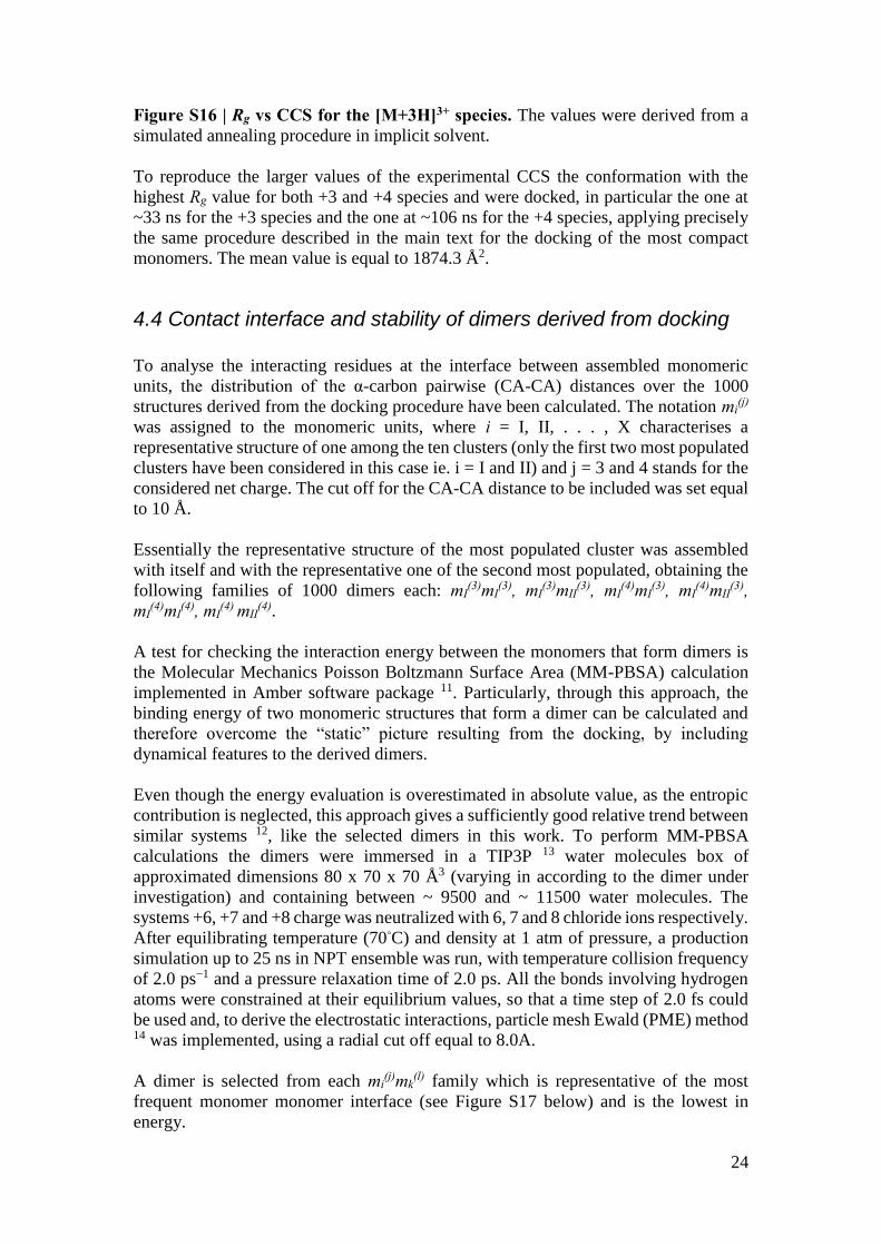
24
Figure S16 | Rg vs CCS for the [M+3H]3+ species. The values were derived from a
simulated annealing procedure in implicit solvent.
To reproduce the larger values of the experimental CCS the conformation with the
highest Rg value for both +3 and +4 species and were docked, in particular the one at
~33 ns for the +3 species and the one at ~106 ns for the +4 species, applying precisely
the same procedure described in the main text for the docking of the most compact
monomers. The mean value is equal to 1874.3 Å2.
4.4 Contact interface and stability of dimers derived from docking
To analyse the interacting residues at the interface between assembled monomeric
units, the distribution of the α-carbon pairwise (CA-CA) distances over the 1000
structures derived from the docking procedure have been calculated. The notation mi(j)
was assigned to the monomeric units, where i = I, II, . . . , X characterises a
representative structure of one among the ten clusters (only the first two most populated
clusters have been considered in this case ie. i = I and II) and j = 3 and 4 stands for the
considered net charge. The cut off for the CA-CA distance to be included was set equal
to 10 Å.
Essentially the representative structure of the most populated cluster was assembled
with itself and with the representative one of the second most populated, obtaining the
following families of 1000 dimers each: mI(3)mI
(3), mI(3)mII
(3), mI(4)mI
(3), mI(4)mII
(3),
mI(4)mI
(4), mI(4) mII
(4).
A test for checking the interaction energy between the monomers that form dimers is
the Molecular Mechanics Poisson Boltzmann Surface Area (MM-PBSA) calculation
implemented in Amber software package 11. Particularly, through this approach, the
binding energy of two monomeric structures that form a dimer can be calculated and
therefore overcome the “static” picture resulting from the docking, by including
dynamical features to the derived dimers.
Even though the energy evaluation is overestimated in absolute value, as the entropic
contribution is neglected, this approach gives a sufficiently good relative trend between
similar systems 12, like the selected dimers in this work. To perform MM-PBSA
calculations the dimers were immersed in a TIP3P 13 water molecules box of
approximated dimensions 80 x 70 x 70 Å3 (varying in according to the dimer under
investigation) and containing between ~ 9500 and ~ 11500 water molecules. The
systems +6, +7 and +8 charge was neutralized with 6, 7 and 8 chloride ions respectively.
After equilibrating temperature (70◦C) and density at 1 atm of pressure, a production
simulation up to 25 ns in NPT ensemble was run, with temperature collision frequency
of 2.0 ps−1 and a pressure relaxation time of 2.0 ps. All the bonds involving hydrogen
atoms were constrained at their equilibrium values, so that a time step of 2.0 fs could
be used and, to derive the electrostatic interactions, particle mesh Ewald (PME) method 14 was implemented, using a radial cut off equal to 8.0A.
A dimer is selected from each mi(j)mk
(l) family which is representative of the most
frequent monomer monomer interface (see Figure S17 below) and is the lowest in
energy.

25
Figure S17 | xy projection of the distributions of the α-carbon pairwise distances.
The two upper, middle and lower figures are related to the [2M+6H]6+, [2M+7H]7+ and
[2M+8H]8+ species respectively. In particular the figures A, B, C, D, E and F refer to
families of docked monomers named mI(3)mI
(3), mI(3)mII
(3), mI(4)mI
(3), mI(4)mII
(3), mI(4)mI
(4),
and mI(4) mII
(4) respectively.
4.4.1 Breakdown of the contributions to the binding energy of representative dimers
A B C D E F
Hydrophobic (kcal/mol)
-6.8 -8.7 -7.4 -6.2 -10.4 -4.9
Hydrophilic (kcal/mol)
103.6 13.0 21.6 -27.7 49.9 -66.9
Table ST4 | CCS Hydrophobic and hydrophilic contributions to the solvation
energy of the dimers representative structures. The hydrophobic and hydrophilic
contributions are derived from surface area (SA) and Poisson-Boltzmann (PB)
approach respectively, along the MM-PBSA procedure. Letters A, B, C, D, E and F
refer to the representative dimers of the families mI(3)mI
(3), mI(3)mII
(3), mI(4)mI
(3),
mI(4)mII
(3), mI(4)mI
(4), and mI(4) mII
(4) respectively.
26
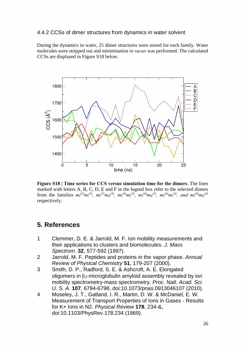
4.4.2 CCSs of dimer structures from dynamics in water solvent
During the dynamics in water, 25 dimer structures were stored for each family. Water
molecules were stripped out and minimisation in vacuo was performed. The calculated
CCSs are displayed in Figure S18 below.
Figure S18 | Time series for CCS versus simulation time for the dimers. The lines
marked with letters A, B, C, D, E and F in the legend box refer to the selected dimers
from the families mI(3)mI
(3), mI(3)mII
(3), mI(4)mI
(3), mI(4)mII
(3), mI(4)mI
(4), and mI(4)mII
(4)
respectively.
5. References
1 Clemmer, D. E. & Jarrold, M. F. Ion mobility measurements and their applications to clusters and biomolecules. J. Mass Spectrom. 32, 577-592 (1997).
2 Jarrold, M. F. Peptides and proteins in the vapor phase. Annual Review of Physical Chemistry 51, 179-207 (2000).
3 Smith, D. P., Radford, S. E. & Ashcroft, A. E. Elongated
oligomers in 2-microglobulin amyloid assembly revealed by ion mobility spectrometry-mass spectrometry. Proc. Natl. Acad. Sci. U. S. A. 107, 6794-6798, doi:10.1073/pnas.0913046107 (2010).
4 Moseley, J. T., Gatland, I. R., Martin, D. W. & McDaniel, E. W. Measurement of Transport Properties of Ions in Gases - Results for K+ Ions in N2. Physical Review 178, 234-&, doi:10.1103/PhysRev.178.234 (1969).

27
5 Sobott, F., Hernandez, H., McCammon, M. G., Tito, M. A. & Robinson, C. V. A tandem mass spectrometer for improved transmission and analysis of large macromolecular assemblies. Anal. Chem. 74, 1402-1407, doi:10.1021/ac0110552 (2002).
6 Onufriev, A., Bashford, D. & Case, D. A. Exploring protein native states and large-scale conformational changes with a modified generalized born model. Proteins-Structure Function and Bioinformatics 55, 383-394, doi:10.1002/prot.20033 (2004).
7 Feig, M. et al. Performance comparison of generalized born and Poisson methods in the calculation of electrostatic solvation energies for protein structures. Journal of Computational Chemistry 25, 265-284, doi:10.1002/jcc.10378 (2004).
8 Tildesley, M. P. A. a. D. J. Computer simulation of liquids. (Clarendon Press, 1986).
9 Shao, J. Y., Tanner, S. W., Thompson, N. & Cheatham, T. E. Clustering molecular dynamics trajectories: 1. Characterizing the performance of different clustering algorithms. Journal of Chemical Theory and Computation 3, 2312-2334, doi:10.1021/ct700119m (2007).
10 Phillips, J. C. et al. Scalable molecular dynamics with NAMD. Journal of Computational Chemistry 26, 1781-1802, doi:10.1002/jcc.20289 (2005).
11 Kollman, P. A. et al. Calculating Structures and Free Energies of Complex Molecules: Combining Molecular Mechanics and Continuum Models. Accounts Chem. Res. 33, 889-897, doi:10.1021/ar000033j (2000).
12 Gilson, M. K. & Zhou, H. X. Calculation of protein-ligand binding affinities. Annual Review of Biophysics and Biomolecular Structure 36, 21-42, doi:10.1146/annurev.biophys.36.040306.132550 (2007).
13 Jorgensen, W. L., Chandrasekhar, J., Madura, J. D., Impey, R. W. & Klein, M. L. Comparison of Simple Potential Functions for Simulating Liquid Water. J. Chem. Phys. 79, 926-935 (1983).
14 Darden, T., York, D. & Pedersen, L. Particle Mesh Ewald - an n.log(n) Method for Ewald Sums in Large Systems. J. Chem. Phys. 98, 10089-10092 (1993).