supplemental materials © copyright 2018 john e ...aberrations of the rotationally symmetric optical...

OPTI-201/202 G

eometrical and Instrum

ental Optics

© C

opyright 2018 John E. Greivenkam

p25-1

Supplemental Materials

Section 25

Aberrations

OPTI-201/202 G


ental Optics

© C


p

OPTI-201/202 G


ental Optics

© C


p25-2

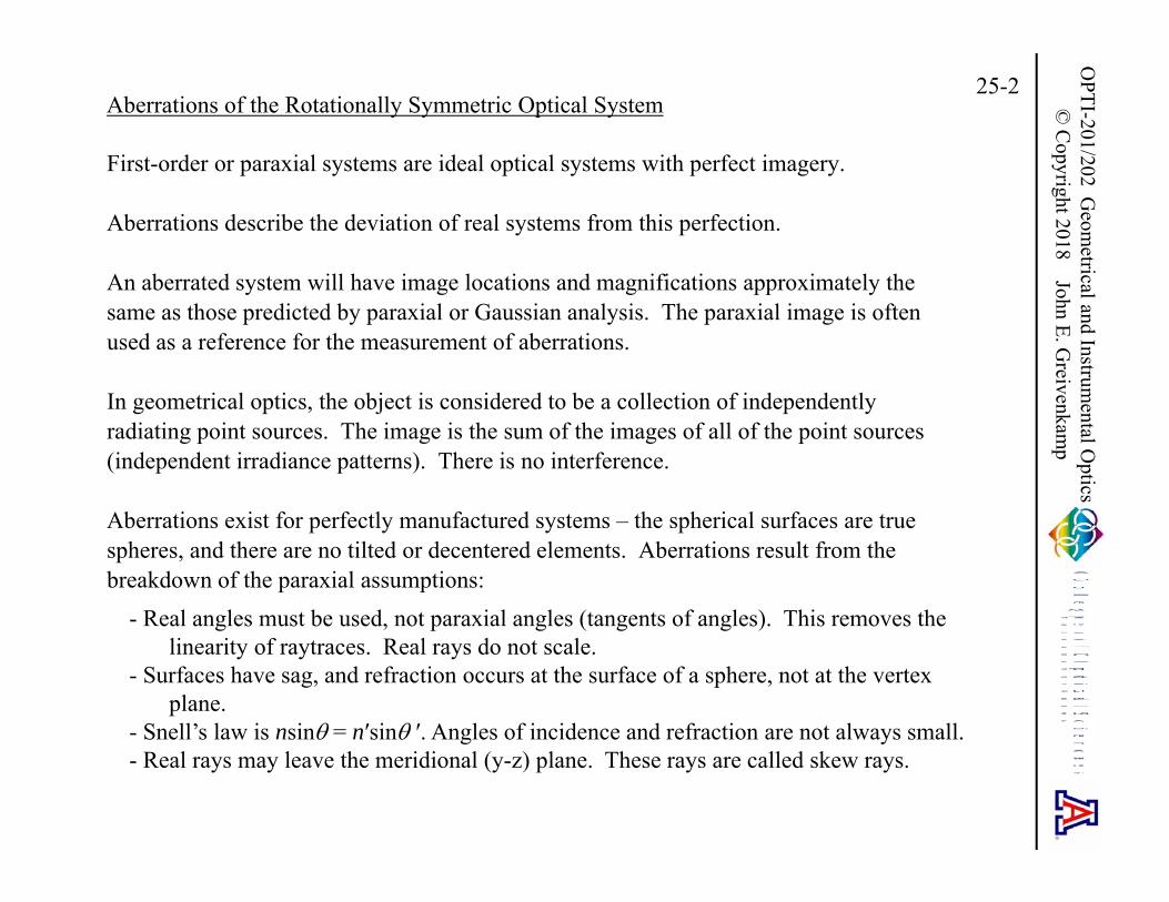
Aberrations of the Rotationally Symmetric Optical System

First-order or paraxial systems are ideal optical systems with perfect imagery.

Aberrations describe the deviation of real systems from this perfection.

An aberrated system will have image locations and magnifications approximately the same as those predicted by paraxial or Gaussian analysis. The paraxial image is often used as a reference for the measurement of aberrations.

In geometrical optics, the object is considered to be a collection of independently radiating point sources. The image is the sum of the images of all of the point sources (independent irradiance patterns). There is no interference.

Aberrations exist for perfectly manufactured systems – the spherical surfaces are true spheres, and there are no tilted or decentered elements. Aberrations result from the breakdown of the paraxial assumptions:

- Real angles must be used, not paraxial angles (tangents of angles). This removes the linearity of raytraces. Real rays do not scale.

- Surfaces have sag, and refraction occurs at the surface of a sphere, not at the vertex plane.

- Snell’s law is nsin = n′sin′. Angles of incidence and refraction are not always small.- Real rays may leave the meridional (y-z) plane. These rays are called skew rays.

OPTI-201/202 G


ental Optics

© C


p25-3

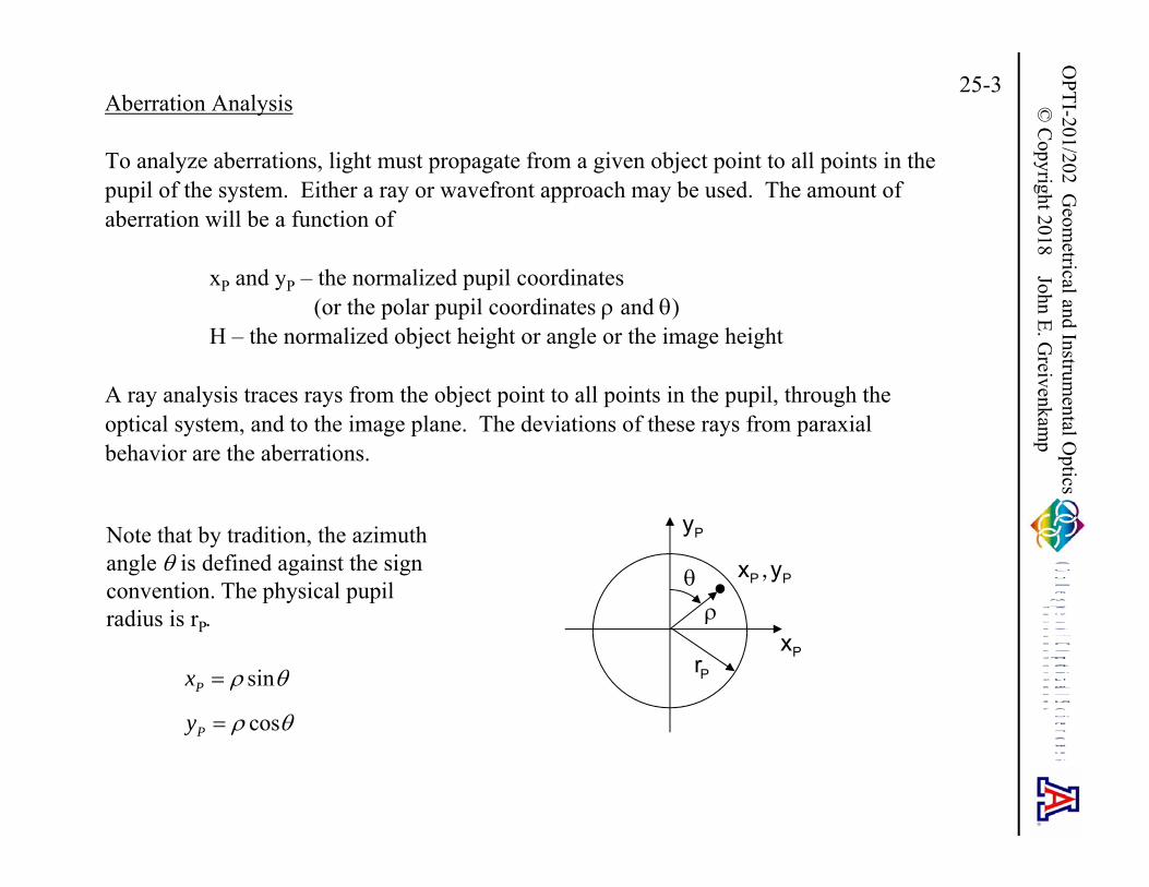
Aberration Analysis

To analyze aberrations, light must propagate from a given object point to all points in the pupil of the system. Either a ray or wavefront approach may be used. The amount of aberration will be a function of

xP and yP – the normalized pupil coordinates (or the polar pupil coordinates and )

H – the normalized object height or angle or the image height

A ray analysis traces rays from the object point to all points in the pupil, through the optical system, and to the image plane. The deviations of these rays from paraxial behavior are the aberrations.

Note that by tradition, the azimuth angle is defined against the sign convention. The physical pupil radius is rP.

sin

cos

P

P

x

y

Px

,P Px y

Py

Pr

OPTI-201/202 G


ental Optics

© C


p25-4

Coordinate System

sin

cos

P

P

x

y

Object

Pupil

Image

x

xP

x′

xP

yP

yPy

x′

y′

y′h

z′

z

OPTI-201/202 G


ental Optics

© C


p25-5

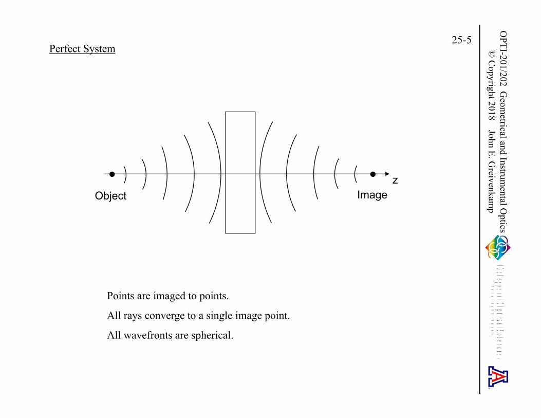
Perfect System

Object Imagez

Points are imaged to points.

All rays converge to a single image point.

All wavefronts are spherical.

OPTI-201/202 G


ental Optics

© C


p25-6

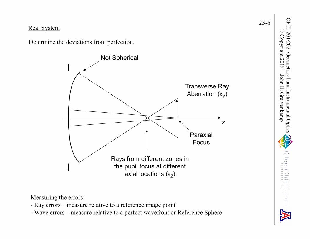
Real System

Determine the deviations from perfection.

Measuring the errors:- Ray errors – measure relative to a reference image point- Wave errors – measure relative to a perfect wavefront or Reference Sphere

Rays from different zones in the pupil focus at different

axial locations (Z)

Transverse RayAberration (Y)

z

ParaxialFocus

Not Spherical

OPTI-201/202 G


ental Optics

© C


p25-7

Reference Image Point

A reference image point is defined by the intersection of the paraxial chief ray and the paraxial image plane. Transverse ray errors X, Y and longitudinal ray errors Z are measured relative to this reference image point. Wavefront errors W are measured in the XP relative to a reference wavefront or reference sphere centered on the reference image point. R is the radius of the reference sphere or the image distance. A positive wavefront error is shown.

P, PW x y

Y P, Px y

Z

Reference WavefrontAberrated Wavefront

XP

R

ReferenceImage Point

z

ParaxialImage Plane

Pr

Both the wavefront error and the ray errors are measured as a function of the pupil coordinates for a particular object point.

OPTI-201/202 G


ental Optics

© C


p25-8

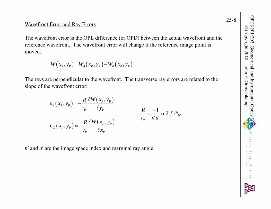
Wavefront Error and Ray Errors

The wavefront error is the OPL difference (or OPD) between the actual wavefront and the reference wavefront. The wavefront error will change if the reference image point is moved.

The rays are perpendicular to the wavefront. The transverse ray errors are related to the slope of the wavefront error:

n′ and u′ are the image space index and marginal ray angle.

, , ,P P A P P R P PW x y W x y W x y

,, P P

Y P PP P

W x yRx yr y

,, P P

X P PP P

W x yRx yr x

1 2 /#WP

R fr n u

OPTI-201/202 G


ental Optics

© C


p25-9

Tangential and Sagittal Rays

By rotational symmetry, only object points in the meridional plane need be considered. A skew ray leaves the meridional plane and intersects a general point in the pupil. Two special sets of rays are used for aberration analysis.

Tangential rays or meridional rays intersect the pupil at xP = 0.

Sagittal rays or transverse rays intersect the pupil at yP = 0.

Object

Pupil

Px Py

z

Px 0

Object

Pupil

Px Py

z

Py 0

OPTI-201/202 G


ental Optics

© C


p25-10

Wave Fans and Ray Fans

Wave fans are plots of the wavefront error for the tangential and sagittal sets of rays.

Ray fans (or ray intercept curves) plot the transverse ray error. The tangential ray fan plots Y versus yP for xP = 0. The sagittal ray fan plots X versus xP for yP = 0.

x

y

X

Y

ReferenceImage Point

Actual Ray

Position Py

Y

1-1

40

-40

Px

X

1-1

40

-40

Example: Spherical Aberration

OPTI-201/202 G


ental Optics

© C


p25-11

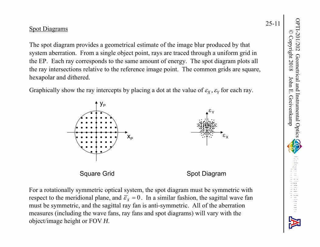
Spot Diagrams

The spot diagram provides a geometrical estimate of the image blur produced by that system aberration. From a single object point, rays are traced through a uniform grid in the EP. Each ray corresponds to the same amount of energy. The spot diagram plots all the ray intersections relative to the reference image point. The common grids are square, hexapolar and dithered.

Graphically show the ray intercepts by placing a dot at the value of X , Y for each ray.

Px

Py

Square Grid

.... ..

....... ... .

..

... ..... ..

.

... ............ .

..... ....... ... .... ..... ......

X

Y.. ... ...... ....

.....

... ............... .. ....... ... .... ..... ............... .. .. .....

.. ... .

...........

..

.. .. ..

....

Spot Diagram

For a rotationally symmetric optical system, the spot diagram must be symmetric with respect to the meridional plane, and . In a similar fashion, the sagittal wave fan must be symmetric, and the sagittal ray fan is anti-symmetric. All of the aberration measures (including the wave fans, ray fans and spot diagrams) will vary with the object/image height or FOV H.

0X

OPTI-201/202 G


ental Optics

© C


p25-12

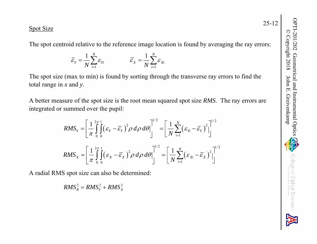
Spot Size

The spot centroid relative to the reference image location is found by averaging the ray errors:

The spot size (max to min) is found by sorting through the transverse ray errors to find the total range in x and y.

A better measure of the spot size is the root mean squared spot size RMS. The ray errors are integrated or summed over the pupil:

A radial RMS spot size can also be determined:

1

1 N

Y YiiN

1

1 N

X XiiN

1/ 2 1/ 22 1

2 2

10 0

1 1 N

Y Y Y Yi Yi

RMS d dN

1/ 2 1/ 22 1

2 2

10 0

1 1 N

X X X Xi Xi

RMS d dN

2 2 2R Y XRMS RMS RMS

OPTI-201/202 G


ental Optics

© C


p25-13

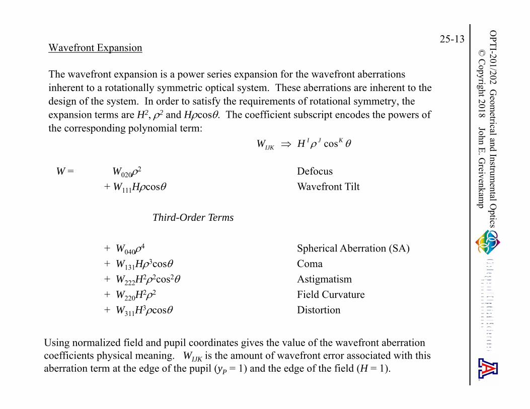
Wavefront Expansion

The wavefront expansion is a power series expansion for the wavefront aberrations inherent to a rotationally symmetric optical system. These aberrations are inherent to the design of the system. In order to satisfy the requirements of rotational symmetry, the expansion terms are H2, 2 and Hcos. The coefficient subscript encodes the powers of the corresponding polynomial term:

cosI J KIJKW H

W = W0202 Defocus+ W111Hcos Wavefront Tilt

Third-Order Terms

+ W0404 Spherical Aberration (SA)+ W131H3cos Coma+ W222H22cos2 Astigmatism + W220H22 Field Curvature+ W311H3cos Distortion

Using normalized field and pupil coordinates gives the value of the wavefront aberration coefficients physical meaning. WIJK is the amount of wavefront error associated with this aberration term at the edge of the pupil (yP = 1) and the edge of the field (H = 1).

OPTI-201/202 G


ental Optics

© C


p25-14

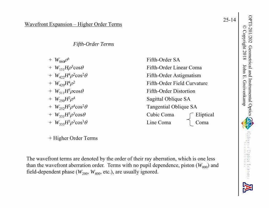
Wavefront Expansion – Higher Order Terms

Fifth-Order Terms

+ W0606 Fifth-Order SA+ W151H5cos Fifth-Order Linear Coma+ W422H42cos2 Fifth-Order Astigmatism+ W420H42 Fifth-Order Field Curvature+ W511H5cos Fifth-Order Distortion+ W250H24 Sagittal Oblique SA+ W252H24cos2 Tangential Oblique SA+ W331H33cos Cubic Coma Eliptical+ W333H33cos3 Line Coma Coma

+ Higher Order Terms

The wavefront terms are denoted by the order of their ray aberration, which is one less than the wavefront aberration order. Terms with no pupil dependence, piston (W000) and field-dependent phase (W200, W400, etc.), are usually ignored.

OPTI-201/202 G


ental Optics

© C


p25-15

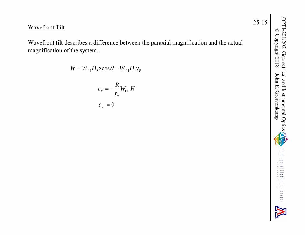
Wavefront Tilt

Wavefront tilt describes a difference between the paraxial magnification and the actual magnification of the system.

111 111cos PW W H W H y

111YP

R W Hr

0X

OPTI-201/202 G


ental Optics

© C


p25-16

Defocus

In a system with defocus W020, the actual image plane is displaced from the paraxial image plane. More importantly, defocus allows the image plane or the reference image point to be shifted for aberration balance and better image quality. For example with spherical aberration, a better image is formed on an image plane inside paraxial focus. Recognizing that this shift is a user decision, the notation W20 is used. Defocus is not really an aberration.

Py

Y

1-1

20

-20

Px

X

1-1

20

-20

20W = 1 f/5

2 2 220 20 P PW W W x y

20 202 cos 2Y PP P

R RW W yr r

20 202 sin 2X PP P

R RW W xr r

OPTI-201/202 G


ental Optics

© C


p25-17

Defocus – Image Plane Shift

In a system that has a wavefront error W and transverse ray aberrations Y , X , an image plane shift changes the measured apparent aberration:

z

ParaxialFocus

ShiftedImagePlane

z

20 28 /#zW

f

2208 /#z f W

W W W Y Y Y

X X X

Moving the image plane changes the reference sphere, not the actual wavefront in the XP of the system.

OPTI-201/202 G


ental Optics

© C


p25-18

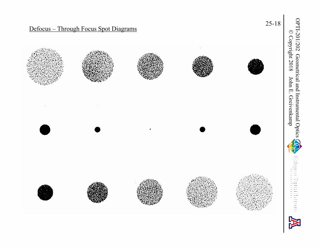
Defocus – Through Focus Spot Diagrams

OPTI-201/202 G


ental Optics

© C


p25-19

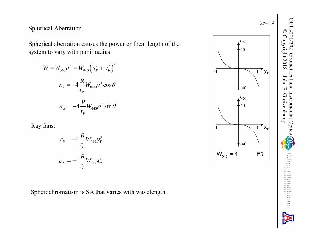
Spherical Aberration

Spherical aberration causes the power or focal length of the system to vary with pupil radius.

Py

Y

1-1

40

-40

Px

X

1-1

40

-40

040W = 1 f/5

24 2 2040 040 P PW W W x y

30404 cosY

P

R Wr

30404 sinX

P

R Wr

Ray fans:

30404Y P

P

R W yr

30404X P

P

R W xr

Spherochromatism is SA that varies with wavelength.

OPTI-201/202 G


ental Optics

© C


p25-20

Transverse and Longitudinal SA

The longitudinal aberration LA is the distance from paraxial focus to marginal focus (where the real marginal ray crosses the axis). The longitudinal ray errors z for SA are quadratic with yP. The real marginal ray angle is U′.

z

Z

LA

TA

MarginalFocus

ParaxialFocus

2 204016 /#Z Pf W y

tanTA LA U

1Y PTA y

Z

Py

LA

1

The transverse aberration TA is the transverse ray error from the top of the pupil:

OPTI-201/202 G


ental Optics

© C


p25-21

Spherical Aberration and Defocus

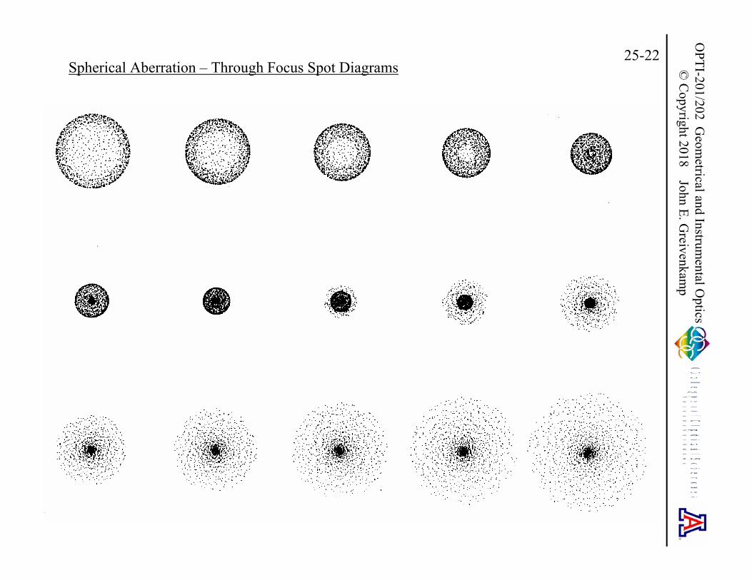
The image plane can be shifted from paraxial focus to obtain better image quality in the presence of SA. Focus criteria include mid focus, minimum RMS spot size, and minimum circle (where the marginal ray crosses the caustic).

MIDz

MINz MARGINALz

RMSz

LA

TA

MarginalFocus

ParaxialFocus

z

Caustic 2

04016 /#LA f W

Mid focus:

Min RMS:

Min circle:

Marginal focus:

20 040W W .5z LA

20 0401.33W W

20 0401.5W W

20 0402W W

.67z LA

.75z LA

z LA

Mid focus corresponds to the minimum wavefront variance condition which is optimum for viewing isolated point sources such as stars. This condition is used for designing telescopes.

OPTI-201/202 G


ental Optics

© C


p25-22

Spherical Aberration – Through Focus Spot Diagrams

OPTI-201/202 G


ental Optics

© C


p25-23

Spherical Aberration – Spot Diagrams at Focus Positions

Marginal Focus

Minimum CircleMinimum RMS

Spot SizeMid Focus

Minimum Wavefront Variance

Paraxial Focus

Square Grid

OPTI-201/202 G


ental Optics

© C


p25-24

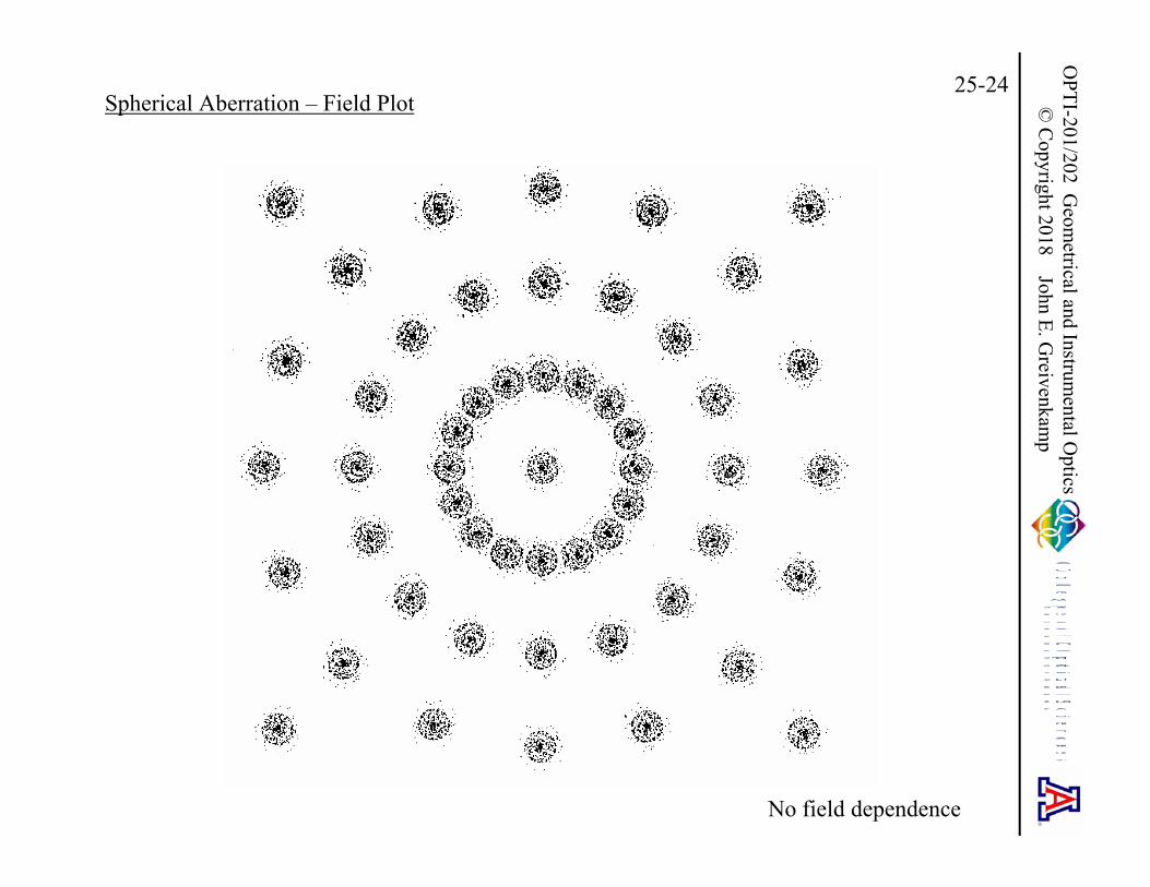
Spherical Aberration – Field Plot

No field dependence

OPTI-201/202 G


ental Optics

© C


p25-25

Spherical Aberration and Lens Bending

The power of a thin lens depends on the difference in the curvatures of its two surfaces:

The lens can be bent without changing its power. However, the aberrations of the lens do change with the bending.

1 21n C C

Smith – Modern Optical Engineering

This plot is for an object at infinity in visible light (n about 1.5). The stop is at the lens. The spherical aberration is minimized for a bending that is approximately convex-plano. The coma is also zero at this bending.

A positive thin lens has positive SA (W040 > 0), independent of lens bending. Bending can only change the magnitude of the SA. This is called undercorrected SA and is the situation shown in all the figures.

OPTI-201/202 G


ental Optics

© C


p25-26

Lens Bending and Minimum SA

The minimum spherical aberration occurs when the light is bent the same amount at each lens surface.

Object at Infinity:

Convex-Plano Plano-Convex

In the plano-convex configuration, all of the ray bending occurs at one surface. In the convex-plano configuration, the ray bending is split between the surfaces. This minimizes the angles of incidence at the surfaces and makes the situation as close to paraxial as possible. This is directly analogous to the angle of minimum deviation for a refracting prism.

There is no bending that completely eliminates spherical aberration. It can only be minimized. Different object/image conjugates require different bendings to minimize spherical aberration.

The optimum shape varies with index. At high index, as is often found in the IR, the best shape is a meniscus.

The other aberrations also vary with the bending of the lens.

Previously Covered

OPTI-201/202 G


ental Optics

© C


p25-27

Spherical Aberration and Finite Congugates

At finite image conjugates, a bi-convex singlet is required to minimize spherical aberration. The particular shape depends on the magnification. At 1:1 imaging, an equiconvex lens is used.

A trick to further minimize spherical aberration is to split the biconvex lens into two plano-convex lenses and then flip each of the lenses:

This final vertex-to-vertex arrangement uses two lenses in their infinite conjugate minimum spherical aberration configuration. Much less spherical aberration results than in the bi-convex solution. The focal lengths of the two lenses can be changed to match the object and image conjugates. This solution is also sometimes used in fast condenser lenses.

z

z

z

Previously Covered

OPTI-201/202 G


ental Optics

© C


p25-28

Coma

Coma results when the magnification of the system varies with pupil position. An asymmetric blur is produced as the entire image blur is to one side of the paraxial image location. The image blur increases linearly with image height H.

Py

Y

1-1

30

-30

Px

X

1-1

30

-30

131W = 1 f/5H = 1

3131 cosW W H

2131 2 cos2Y

P

R W Hr

2131 sin 2X

P

R W Hr

21313Y P

P

R W H yr

0X

Ray fans:

OPTI-201/202 G


ental Optics

© C


p25-29

Coma – Spot Diagram

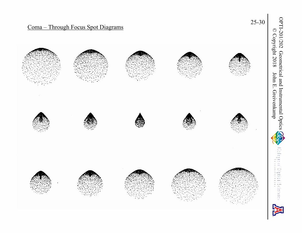
For a given object point, each annular zone in the pupil maps to a displaced circle of light in the image blur. The blur is contained in a 60 degree wedge, and about 55% of the light is contained in the first third of the pattern. Depending on the sign of the coma, the pattern can flare towards (W131 > 0) or away from the optical axis (W131 < 0). H is assumed to represent a positive image height.

TC

SC

SC

60°ParaxialImagePoint

Tangential coma CT and sagittal coma CSare two measures of coma:

1313TP

RC Wr

131SP

RC Wr

For a thin lens, coma varies with lens bending and the stop position. For any bending, there is a stop location that eliminates coma. This is the natural stop position.

OPTI-201/202 G


ental Optics

© C


p25-30

Coma – Through Focus Spot Diagrams

OPTI-201/202 G


ental Optics

© C


p25-31

Coma – Field Plot

OPTI-201/202 G


ental Optics

© C


p25-32

Astigmatism

In a system with astigmatism, the power of the optical system in horizontal and vertical meridians is different as a function of image height.

Py

Y

1-1

20

-20

Px

X

1-1

20

-20

222W = 1 f/5H = 1

2 2 2 2 2222 222cos PW W H W H y

22222Y P

P

R W H yr

0X

With positive astigmatism, light from a vertical meridian is focused closer to the lens than light through the horizontal meridian. Each object point produces two perpendicular line images. These are the tangential focus and the sagittal focus.

Smith – Modern Optical Engineering

OPTI-201/202 G


ental Optics

© C


p25-33

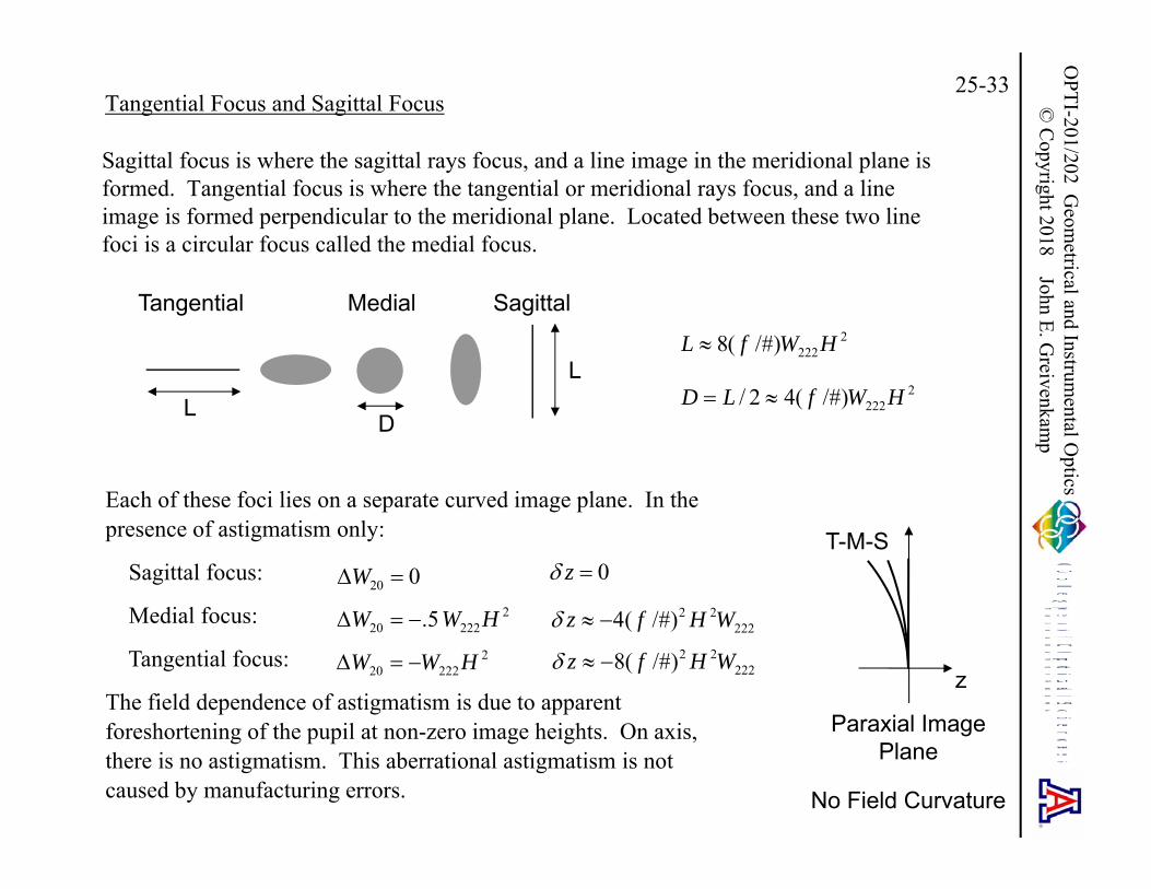
Tangential Focus and Sagittal Focus

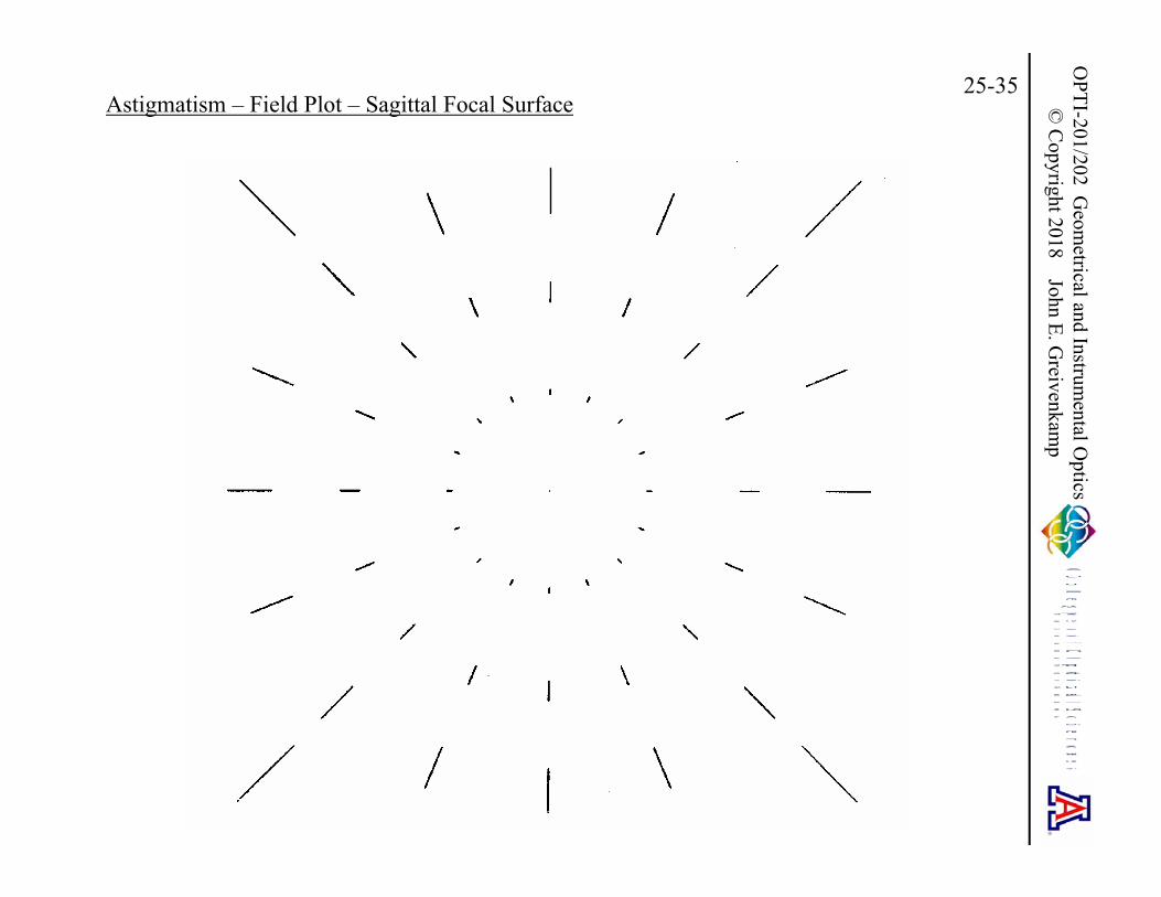
Sagittal focus is where the sagittal rays focus, and a line image in the meridional plane is formed. Tangential focus is where the tangential or meridional rays focus, and a line image is formed perpendicular to the meridional plane. Located between these two line foci is a circular focus called the medial focus.

LD

L

SagittalMedialTangential2

2228( /#)L f W H

2222/ 2 4( /#)D L f W H

Each of these foci lies on a separate curved image plane. In the presence of astigmatism only:

Sagittal focus:

Medial focus:

Tangential focus:

The field dependence of astigmatism is due to apparent foreshortening of the pupil at non-zero image heights. On axis, there is no astigmatism. This aberrational astigmatism is not caused by manufacturing errors.

20 0W 0z

220 222.5W W H 2 2

2224( /#)z f H W 2

20 222W W H 2 22228( /#)z f H W

T-M-S

Paraxial ImagePlane

No Field Curvature

z

OPTI-201/202 G


ental Optics

© C


p25-34

Astigmatism – Through Focus Spot Diagrams

MedialTangential Sagittal

OPTI-201/202 G


ental Optics

© C


p25-35

Astigmatism – Field Plot – Sagittal Focal Surface

OPTI-201/202 G


ental Optics

© C


p25-36

Astigmatism – Field Plot – Medial Focal Surface

OPTI-201/202 G


ental Optics

© C


p25-37

Astigmatism – Field Plot – Tangential Focal Surface

OPTI-201/202 G


ental Optics

© C


p25-38

Visual Astigmatism

The astigmatism present in a rotationally symmetric optical system does not exist on axis or at zero field height. This asymmetry in power results from the apparent foreshortening of the pupil at non-zero fields of view. When the circular pupil is viewed at an oblique angle, it will appear elliptical in shape.

Visual astigmatism, on the other hand, results from imperfections of either the cornea or the crystalline lens of the eye. One or both have a cylindrical component to their shape. As a result, the paraxial power of the eye varies with meridional cross section. Line images result on axis, and this type of error does not vary with field of view. Imperfectly manufactured optical systems may exhibit this same type of error.

The term “astigmatism” is used to describe these two different conditions. To distinguish them, adjectives can be used:

- Aberrational astigmatism- Visual astigmatism or axial astigmatism

OPTI-201/202 G


ental Optics

© C


p25-39

Field Curvature

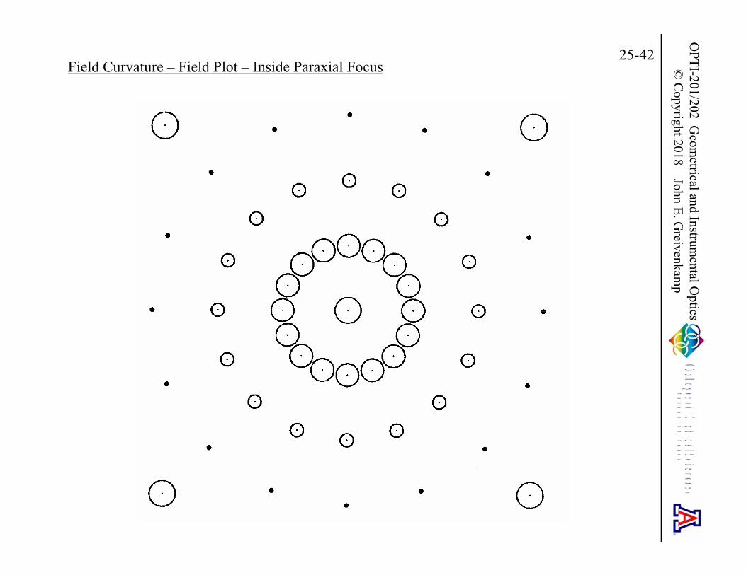
Field curvature characterizes the natural tendency of optical systems to have curved image planes. A positive singlet has an inward bending image surface.

Py

Y

1-1

20

-20

Px

X

1-1

20

-20

220W = 1 f/5H = 1

2 2 2 2 2220 220 P PW W H W H x y

22202Y P

P

R W H yr

22202X P

P

R W H xr

A perfect image is formed on a curved surface, and the image blur at the paraxial image plane increases as H2. A compromise flat image plane that reduces the average image blur occurs inside paraxial focus.

ImageBlur

ImageBlur

z

z z

OPTI-201/202 G


ental Optics

© C


p25-40

Field Curvature – Petzval Surface

The field curvature is a bias curvature for the astigmatic image surfaces.

Sagittal surface:

Medial surface:

Tangential surface:

Petzval surface:

While not a good image surface, the Petzval surface represents the fundamental field curvature of the system. It depends only on the construction parameters of the system: surface curvatures and element indices of refraction.

These four image surfaces are equally spaced and occur in the same relative order: T-M-S-P or P-S-M-T. The best image quality occurs at medial focus. An artificially flattened field or medial surface can be obtained by balancing astigmatism and field curvature.

220 220W W H

2 220 220 222.5W W H W H

2 220 220 222W W H W H

2 220 220 222.5W W H W H

OPTI-201/202 G


ental Optics

© C


p25-43

Distortion

Distortion occurs when image magnification varies with the image height H. Straight lines in the object are mapped to curved lines in the image. Points still map to points, so there is no image blur associated with distortion.

3 3311 311cos PW W H W H y

3311Y

P

R W Hr

0X

Distortion is a quadratic magnification error, and the image point position is displaced in a radial direction.

The transverse ray fans for wavefront tilt and distortion both are constant with respect to yP. These two aberration terms can be distinguished by their different field or Hdependence: linear for wavefront tilt and cubic for distortion.

OPTI-201/202 G


ental Optics

© C


p25-44

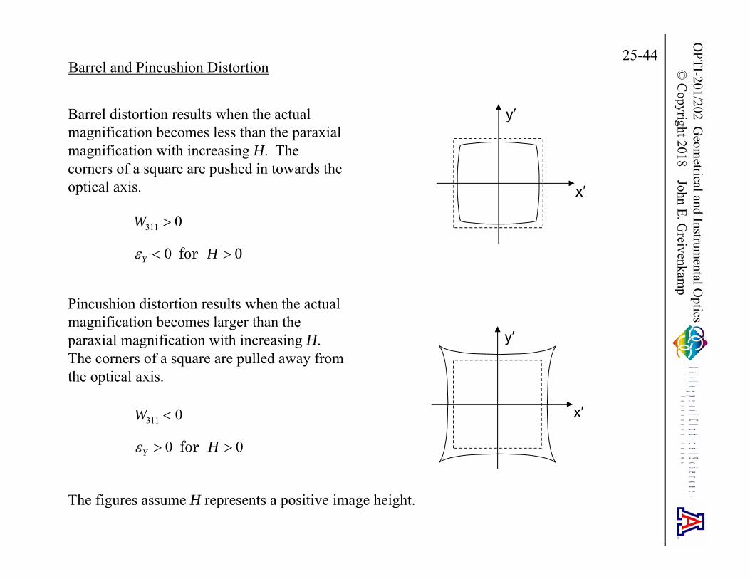
Barrel and Pincushion Distortion

The figures assume H represents a positive image height.

Barrel distortion results when the actual magnification becomes less than the paraxial magnification with increasing H. The corners of a square are pushed in towards the optical axis.

Pincushion distortion results when the actual magnification becomes larger than the paraxial magnification with increasing H. The corners of a square are pulled away from the optical axis.

311 0W

0 0Y H for

311 0W

0 0Y H for

x

y

x

y

OPTI-201/202 G


ental Optics

© C


p25-45

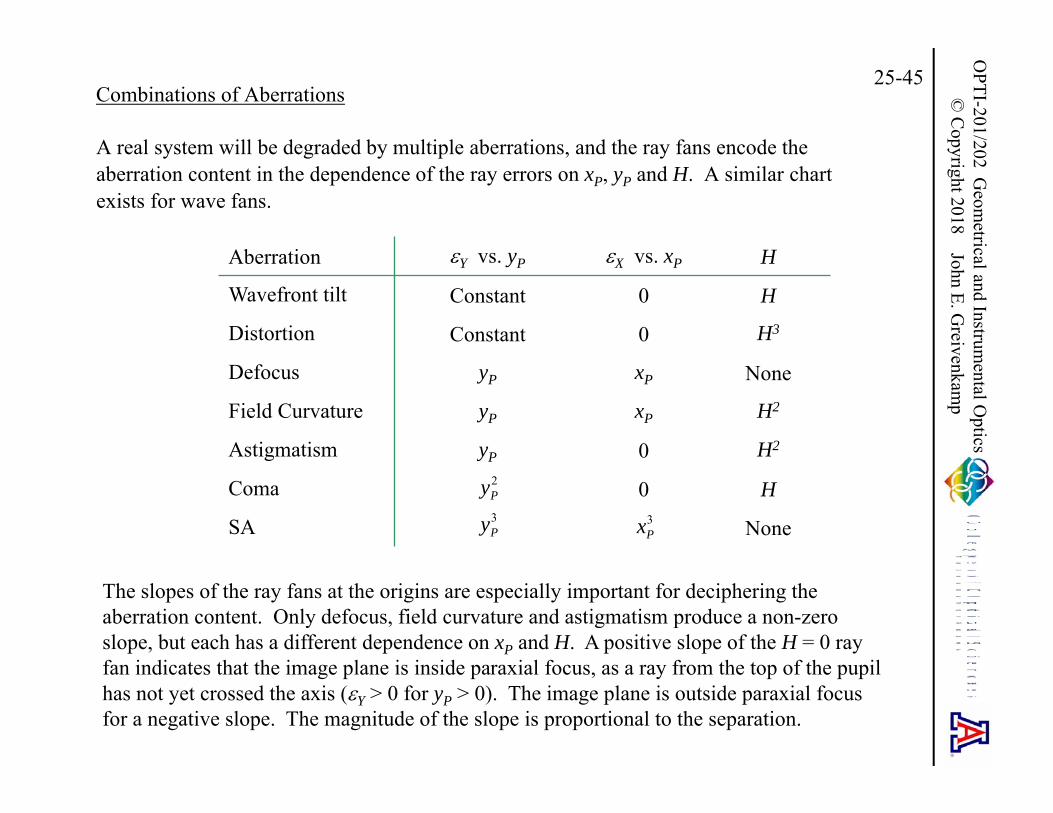
Combinations of Aberrations

A real system will be degraded by multiple aberrations, and the ray fans encode the aberration content in the dependence of the ray errors on xP, yP and H. A similar chart exists for wave fans.

The slopes of the ray fans at the origins are especially important for deciphering the aberration content. Only defocus, field curvature and astigmatism produce a non-zero slope, but each has a different dependence on xP and H. A positive slope of the H = 0 ray fan indicates that the image plane is inside paraxial focus, as a ray from the top of the pupil has not yet crossed the axis (Y > 0 for yP > 0). The image plane is outside paraxial focus for a negative slope. The magnitude of the slope is proportional to the separation.

Aberration Y vs. yP X vs. xP H

Wavefront tilt Constant 0 H

Distortion Constant 0 H3

Defocus yP xP None

Field Curvature yP xP H2

Astigmatism yP 0 H2

Coma 0 H

SA None

2Py3Py 3

Px

OPTI-201/202 G


ental Optics

© C


p25-46

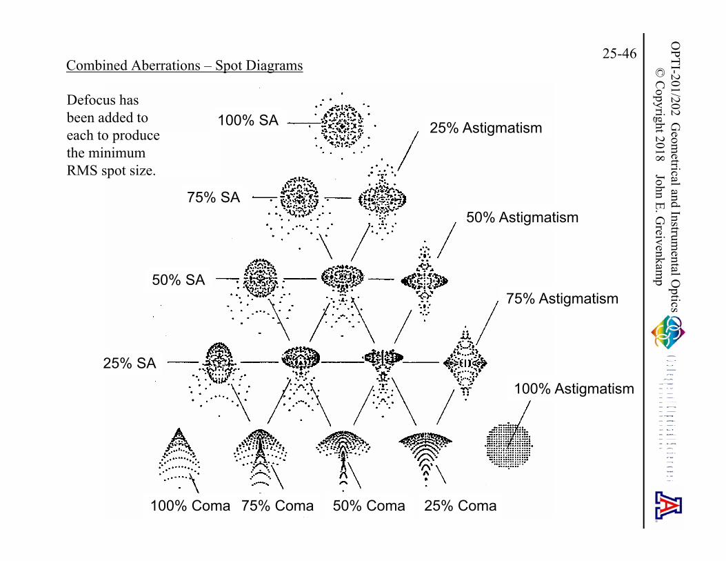
Combined Aberrations – Spot Diagrams

100% SA

75% SA

50% SA

25% SA

25% Astigmatism

100% Astigmatism

75% Astigmatism

50% Astigmatism

100% Coma 75% Coma 50% Coma 25% Coma

Defocus has been added to each to produce the minimum RMS spot size.

OPTI-201/202 G


ental Optics

© C


p25-48

Conics and Aspheres

Because of the ease of fabrication and testing, most optical surfaces are flat or spherical. The introduction of aspheric surfaces provides more optimization variables for aberration correction. Rotational symmetry is maintained.

The first class of aspheric surfaces is generated by rotation of a conic section about the optical axis. Conics are defined by two foci. A source placed at one focus will image without aberration to the other focus. The sag of a conic is given by

2

2 2 1/ 2( )1 (1 (1 ) )

C rs rC r

where C is the base curvature of the surface, r is the radial coordinate and k is the conic constant. Conics are often used as reflecting surfaces.

OPTI-201/202 G


ental Optics

© C


p25-49

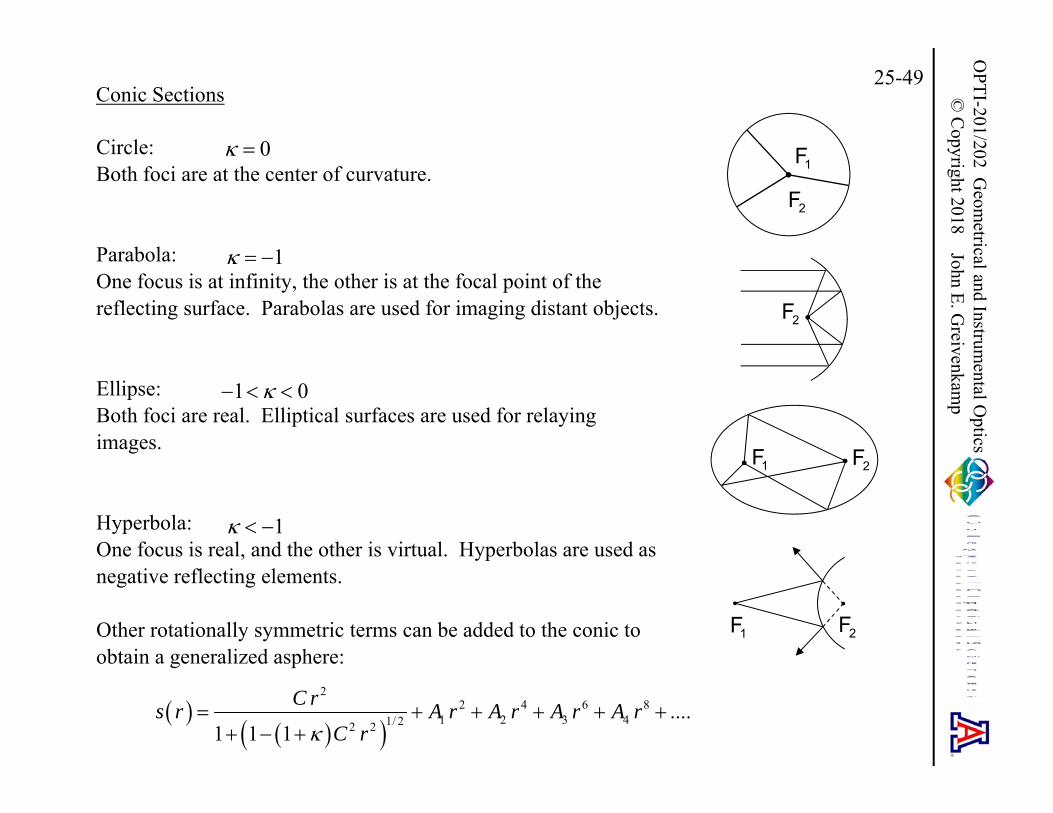
Conic Sections

Circle:Both foci are at the center of curvature.

Parabola:One focus is at infinity, the other is at the focal point of the reflecting surface. Parabolas are used for imaging distant objects.

Ellipse:Both foci are real. Elliptical surfaces are used for relaying images.

Hyperbola:One focus is real, and the other is virtual. Hyperbolas are used as negative reflecting elements.

Other rotationally symmetric terms can be added to the conic to obtain a generalized asphere:

1F

2F

2F

1F 2F

1F 2F

1

1 0

1

0

22 4 6 8

1 2 3 41/ 22 2....

1 1 1

C rs r A r A r A r A rC r

OPTI-201/202 G


ental Optics

© C


p25-50

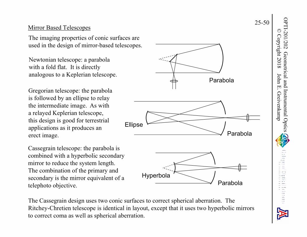
Mirror Based Telescopes

Parabola

ParabolaEllipse

HyperbolaParabola

Newtonian telescope: a parabola with a fold flat. It is directly analogous to a Keplerian telescope.

Gregorian telescope: the parabola is followed by an ellipse to relay the intermediate image. As with a relayed Keplerian telescope, this design is good for terrestrial applications as it produces an erect image.

Cassegrain telescope: the parabola is combined with a hyperbolic secondary mirror to reduce the system length. The combination of the primary and secondary is the mirror equivalent of a telephoto objective.

The imaging properties of conic surfaces are used in the design of mirror-based telescopes.

The Cassegrain design uses two conic surfaces to correct spherical aberration. The Ritchey-Chretien telescope is identical in layout, except that it uses two hyperbolic mirrors to correct coma as well as spherical aberration.

OPTI-201/202 G


ental Optics

© C


p25-51

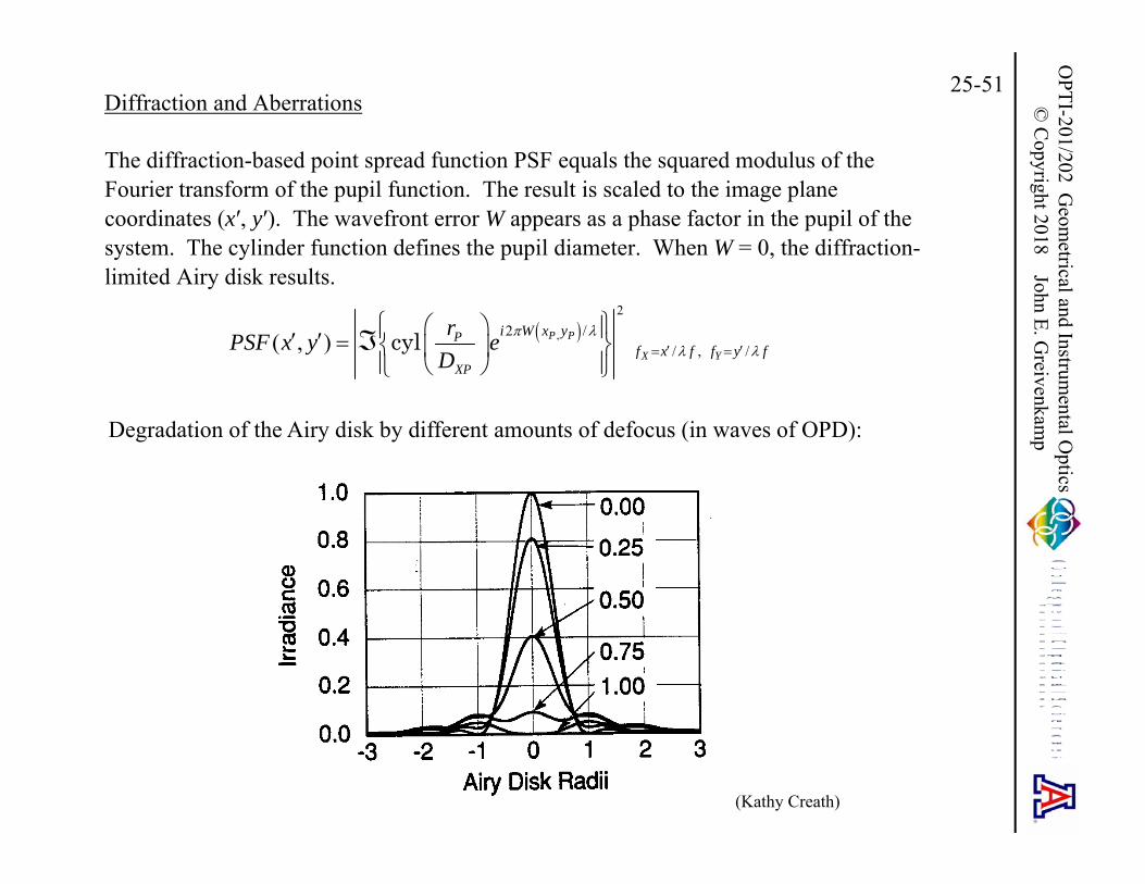
Diffraction and Aberrations

The diffraction-based point spread function PSF equals the squared modulus of the Fourier transform of the pupil function. The result is scaled to the image plane coordinates (x′, y′). The wavefront error W appears as a phase factor in the pupil of the system. The cylinder function defines the pupil diameter. When W = 0, the diffraction-limited Airy disk results.

,

22 /

/ , /( , ) P P

X Y

P

XP

i W x yf x f f y f

rPSF x y eD

cyl

Degradation of the Airy disk by different amounts of defocus (in waves of OPD):

(Kathy Creath)

OPTI-201/202 G


ental Optics

© C


p25-52

Spherical Aberration and Diffraction

Different Amounts of SA (in waves of OPD):

Note that for both SA and defocus, the system is nearly diffraction limited when the introduced wavefront aberration is less than /4. This is the Rayleigh criterion for image quality.

Spherical aberration balanced with an equal and opposite amount of defocus (both in waves of OPD):

These improved spot patterns result from refocusing the image plane to find a “best” focus location.

(Kathy Creath)

OPTI-201/202 G


ental Optics

© C


p25-53

Strehl Ratio

The Strehl ratio SR is a single-number measure of image quality for systems with small amounts of aberration.

The SR has a maximum value of one, and it measures the degradation of the Airy disk. Any reduction of the SR is directly proportional to the wavefront variance. The SR is correlates well with image quality down to values of about 0.5.

0E

r W1.22 f/#

0E

Airy Disk

AberratedAiry Disk

E

SR 0.7

0

0

ESRE

OPTI-201/202 G


ental Optics

© C


p25-54

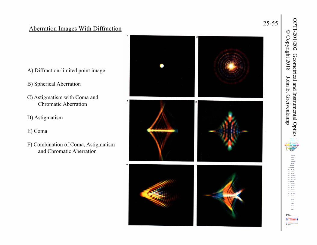
Aberration Images With Diffraction

Images from William H. Price, “The Photographic Lens,” Scientific American, 72-83 (August 1976). The following photomicrographs were taken by Norman Goldberg who was Technical Director of Popular Photography Magazine.

Caption: Lens aberrations can be studied by magnifying the images formed at the focal plane when a point light source is beamed at the lens. In the photomicrographs on the opposite page, made by Norman Goldberg, technical director of Popular Photography, the images are magnified 600 diameters. Ideally the image should be a point (a), but the ideal is usually achieved, as in this case, only when the light source is in line with the axis of the lens. Image (b) exhibits one of the most common lens defects, spherical aberration. Another common defect, astigmatism, accounts for the strong horizontal line in image (c), which also exhibits coma and spherical aberration. Astigmatism shows up in purer form in image (d). If the focus of the lens were moved slightly either forward or back, the astigmatism would produce either a sharp horizontal line or a sharp vertical line. Coma, a familiar type of aberration that arises when the light source is off axis, is depicted in image (e). The final image (f), which combines a complex mixture of coma, astigmatism and chromatic aberration, is typical of the off-axis images produced when fast, modern lenses are used at full aperture. After allowance for the great magnification of the image, however, it is evident that the lens focuses most of the light energy within a very small “blur disk,” which in this case is a circle with a diameter of .03 millimeter.

OPTI-201/202 G


ental Optics

© C


p25-55

Aberration Images With Diffraction

A) Diffraction-limited point image

B) Spherical Aberration

C) Astigmatism with Coma and Chromatic Aberration

D) Astigmatism

E) Coma

F) Combination of Coma, Astigmatism and Chromatic Aberration

supplemental materials © copyright 2018 john e ...aberrations of the rotationally symmetric optical...

Documents