Supervised Damage and Deterioration Detection in Building Structures Using an Enhanced Autoregressive Time-Series Approach

Vahid Reza Gharehbaghi1, Andy Nguyen2, Ehsan Noroozinejad Farsangi3*, T.Y. Yang4

1 Research Scholar, Kharazmi University, Faculty of Civil Engineering, Tehran, Iran 2 A/Professor, University of Southern Queensland, Springfield Campus, Queensland 4030, Australia

3 A/Professor, Graduate University of Advanced Technology, Kerman, Iran 4 Professor, University of British Columbia, Vancouver, Canada

*Corresponding Author, Email: noroozinejad@kgut.ac.ir

Abstract In this paper, a supervised learning approach is introduced for detecting both damage and

deterioration in two building models under ambient and forced vibrations. The coefficients and residuals of autoregressive (AR) time-series models are utilized for extracting features through some statistical indices. Moreover, a novel algorithm called best-uncorrelated features selection (BUFS) is proposed and utilized in order to select the most sensitive and uncorrelated features, which are used as predictors. Accordingly, a common set of predictors capable of detecting both damage and deterioration is established and used in order to form a general pattern of the structural condition. Besides, the BUFS algorithm can also be utilized with other features as well as different types of structures and depicts the most sensitive predictors. The results indicate that the proposed method is capable of detecting damage and deterioration in both models precisely, even in a noisy environment, and the appropriate features are introduced.

Keywords: Autoregressive (AR) time-series; Damage, and deterioration detection; BUFS

algorithm; Supervised learning; Ambient vibration; Forced vibration.

1. Introduction Structural Health Monitoring (SHM) provides valuable information regarding the behavior of

structure by construing the responses, detecting damages, and evaluating the current state. It is worth to note that it was first exploited on behalf of damage diagnosing in the aerospace industries and, after that, penetrated into offshore platform structures [1]. Following that, in the late 1970s, it was similarly practiced in various types of civil engineering structures [1]. As a concise definition, Farrar and Sohn [2] defined SHM as a process of implementing a damage identification strategy in respect of utilization in different structures.

A typical SHM system includes three principal components comprising: a sensor system, a data processing system (including data acquisition, transmission, and storage), and a data interpretation system [3]. The interpretation component includes diagnosis (assessment) and prognosis (prediction) of the structural states attributable to environmental variations. The diagnosis illustrates the onset of damage as well as its location and extent. This section can be

divided into passive diagnosis (e.g., passive sensors such as strain gauges) and active diagnosis (e.g., actuators and smart sensors) [4]. Likewise, the prognosis section defines the kind of damage, assessing the response patterns of structure, and predicting the remaining life. Therefore, the combination of these components empowers the engineers to select and perform an appropriate SHM system on a particular infrastructure. In a sentence, an SHM system aims to -diagnose and prognose different sorts of damage in a monitored structure. The sooner and more accurate this evaluation is done, the lower the cost of maintenance in the future will be.

Figure.1 Interpretation of damage [1]

Damage detection can be carried out by either using models or signal analysis. In a model-based approach, the damage is identified by tracking changes in the simulated measurements from the structural models [5]. As a definition, a model is an assumed relationship between the input and output variables of a system, taking the (known or assumed) properties of that system into account [6]. In other words, in model-based problems, specific parameters of a finite element model (FEM) are updated in order to identify damage [7-10]. However, these methods have some restitutions, such as requiring prior information concerning boundary conditions, damage location, or material properties [1]. Additionally, an optimization problem is prone to ill-conditioning, meaning that the existence, uniqueness, and stability of a solution of the inverse problem cannot be guaranteed. On the other hand, signal-based methods, which are based on statistical analysis, evaluate the response of the structure directly, and herewith they do not require further knowledge as regards the system conditions or properties [11-15].

Concerning structure excitation sorts, the input vibrations imposed are categorized into two

dominant types: (a) ambient vibrations; and (b) forced vibrations [16]. Firstly, the ambient loads are non-deterministic, which can be described as stochastic processes such as random white noise. By applying signal-processing techniques, it is possible to separate the stochastic part of the response from the deterministic component associated with the behavior of the structure. One of the most common techniques is the Random Decrement Technique (RDT), which is used to estimate cross-correlation functions and free-response decays [17]. Secondly, forced vibration tests may require enormous force-generating instruments to produce significant and useful response amplitudes [1]. Additionally, due to the high-cost burden of generating vibration in existing structures, and anticipated hazards, the application of low-cost ambient vibration tests has increased during recent years [18-23].

Evaluation of output responses is carried out in different domains. Regarding the domain, analyzing the structural responses can be carried out in distinctive domains, namely frequency-

DiagnosisIdentificationLocalization

Severity evaluation

PrognosisClassificationAssessment

Lifecycle prediction

domain, time-domain, or time-frequency domain. Some of the more common methods using in frequency-domain are Fourier Transform (FT), Fast Fourier Transform (FFT), and Frequency Response Analysis (FRA), practiced by numerous researchers [24, 25]. Likewise, Short-Time Fourier Transform (STFT), wavelet analysis, Empirical Mode Decomposition (EMD) and Hilbert Spectral Analysis (HSA) are considered time-frequency analyzing tools [26-28].

Moreover, various studies have carried out using time-series models. For instance, Lautour and

Omenzetter [29] utilized Autoregressive (AR) models for detecting damage in two experimental building models. They considered coefficients of AR models to be sensitive features and applied a trained Artificial Neural Network (ANN) for classifying different damage cases. In another study, Hu and Xuan [30] introduced a threshold based on the residual series standard deviation of a nonlinear auto-regressive moving average (ARMA) model in order to separate damaged from undamaged states. Furthermore, Farahani et al. [31] identified damage in three-dimensional FE models of a bridge using autoregressive with exogenous input (ARX) models and a damage-sensitive feature (DSF). Lakshmi and Rao [32] localized single and multiple damages in a simply supported beam and a three-story bookshelf benchmark structure using AR–ARX model and a new damage index based on the probability density function. Monavari et al. [33] evaluated deterioration in 3- and 20-story reinforced concrete (RC) frames excited under ambient vibrations using Autoregressive Residuals. They presented a new criterion for estimating the best-fit model order of AR time-series called (BMO). They also practiced the coefficients of (AR) time-series model and statistical hypotheses of Two-sample t-tests to detect deterioration in a structure [34].

Generally, deterioration occurs in a prolonged and progressive process, majorly caused by

environmental variations such as humidity, temperature, or corrosion. Thus, it primarily takes a couple of years to have considerable influence on the structure and requires a more precise method to be distinguished. In contrast, the damage is caused by severe changes in the structure geometry and materials as well as connections, including removing beams, braces, or loosening bolts in connections. Although many papers developed various methods for detecting damage, evaluating structures in early stages before the occurrence of damage is indispensable which is relatively neglected as a widening gap in the realm of SHM. As a consequence, this study focuses on detecting both deterioration and damage in the time domain regarding two building models, which are under forced and ambient vibrations.

Thus, the most economical and practical approach in the realm of SHM would be assessing the output only response signals of the structure excited by ambient vibrations. Additionally, the majority of the researchers made their efforts mainly on detecting damage in simple structures such as beams, frames or single bay bridges. As a result of that, in this study, authors focused on evaluating deterioration in building models, which in them the correlation of story responses is considered a controversial issue.

2. Detection procedure The damage detection procedure in the current study pursues three preliminary steps. At first,

the input signals are issued for pre-processing in order to denoise, normalize, and similarly whiten the input accelerations. Afterward, the pre-processed signals are utilized for building Autoregressive (AR) models and related parameters. The obtained parameters are implemented for extracting distinguishing features via some statistical properties. The feature subset selection is performed by a method called BUFS, which selects the most uncorrelated and sensitive features referred to as predictors. Then, the discriminant classification algorithm is employed to recognize the pattern generated by the predictors. A more detailed explanation of the suggested approach is provided in the following sections.

2.1 Pre-processing The time-series models, such as the AR models, consider data to be stationary while comparing

time history responses, which may occur because of distinctive loading conditions, including different magnitudes or directions [35]. Thus, the recorded acceleration time histories by each sensor are standardized (or normalized) as:

�̃�𝑠𝑖𝑖 =𝑠𝑠𝑖𝑖 − μ𝜎𝜎

(1)

Where �̃�𝑠𝑖𝑖 stands for the normalized signal of 𝑠𝑠𝑖𝑖 with the mean of μ and standard deviation (STD) of 𝜎𝜎. In order to eliminate the noise effects, a digital filter is utilized. These filters are broadly implemented in order to remove specific parts of signals which may be contaminated with noise. The frequency response 𝐻𝐻(𝑤𝑤) in the frequency domain, which is discrete-time Fourier transform of time response ℎ(𝑡𝑡), is considered a key factor for their characteristics. Accordingly, two forms of digital filters are defined based on different types of ℎ(𝑡𝑡) design which are called finite-duration impulse response (FIR) and infinite-duration impulse response (IIR). In the FIR filters, the impulse response is nonzero for only a finite number of samples and in the second type, it has an infinite number of nonzero samples [37]. Even though FIR filters have proven better performance, IIR filters achieve the desired specifications with relatively lower order and fewer parameters [38]. Therefore, in this study, the normalized signals are filtered by an IIR digital low-pass filter named Chebyshev type II with fast computing speed to dwindle the effects of high-frequency contents [36]. Importantly, this type of filter has been practiced in similar SHM purposes by other researchers [33, 39, 40].

Overall, the recorded signals are reciprocally related and, accordingly, it can cause the deviation of results. Hence, in the pre-whitening (or sphering) processing, a linear transformation is implemented to decorrelate signals. This process can be implemented by two popular whitening techniques, namely zero-phase component analysis (ZCA) and Principal component analysis (PCA). The former approach produces whitened signals with more similarities to the genuine variables, and the later generates whitened variables that highly condense the primary variables [41]. Furthermore, implementing these transformations minimizes the cross-correlation between multiple signals.

Mathematically, a whitening matrix, like 𝑊𝑊 is a linear transformation that converts a random d-dimension signal 𝑠𝑠 = (𝑠𝑠1, … , 𝑠𝑠𝑑𝑑) into a new vector 𝑌𝑌 as follows: 𝑌𝑌 = (𝑌𝑌1, … ,𝑌𝑌𝑑𝑑) = 𝑊𝑊𝑠𝑠 (2)

Where 𝑑𝑑 is the number of sensors or channels, 𝑊𝑊 is a 𝑑𝑑 by 𝑑𝑑 whitening matrix, and 𝑌𝑌 indicates the whitened signal vectors like 𝑠𝑠. It is essential to mention that the transformation matrix 𝑊𝑊 causes the original covariance matrix 𝐾𝐾 = 𝑐𝑐𝑐𝑐𝑐𝑐(𝑠𝑠) becomes an identity matrix so that 𝑐𝑐𝑐𝑐𝑐𝑐(𝑌𝑌) = 𝐼𝐼𝑑𝑑 . In other words, all the components of 𝑌𝑌 have unique variance; so, the existence correlations eliminate. Besides, with the decomposition of the covariance matrix 𝐾𝐾 into eigenvectors 𝑈𝑈, and eigenvalues Λ = {𝛾𝛾1,𝛾𝛾2, … 𝛾𝛾𝑑𝑑}, 𝛾𝛾1 ≥ 𝛾𝛾2 ≥ ⋯ ≥ 𝛾𝛾𝑑𝑑 > 0 as:

K = 𝑈𝑈 Λ 𝑈𝑈𝑇𝑇 (3)

It can be deduced that the PCA and ZCA transformation take the form as:

𝑌𝑌𝑃𝑃𝑃𝑃𝑃𝑃 = 𝑊𝑊𝑃𝑃𝑃𝑃𝑃𝑃𝑠𝑠 = Λ−12 𝑈𝑈𝑇𝑇𝑠𝑠 (4)

Consequently, with an additional rotation by 𝑈𝑈, we have:

𝑌𝑌𝑍𝑍𝑃𝑃𝑃𝑃 = 𝑊𝑊𝑍𝑍𝑃𝑃𝑃𝑃𝑠𝑠 = 𝑈𝑈 Λ−12 𝑈𝑈𝑇𝑇𝑠𝑠

(5)

In this study, the ZCA transformation is employed for decorrelating the story responses as well as enhancing the accuracy of detection.

2.2 Processing Once the data is pre-processed, the procured signals are then utilized in Autoregressive (AR)

models. Considering the structural responses to be stationary, the AR model is given by:

𝑠𝑠𝑗𝑗 = �𝛼𝛼𝑖𝑖

𝑝𝑝

𝑖𝑖=1

𝑠𝑠𝑗𝑗−𝑖𝑖 + 𝜀𝜀𝑗𝑗 (6)

Where 𝑠𝑠𝑗𝑗 indicates the normalized acceleration signal at 𝑗𝑗th time interval; 𝜀𝜀𝑗𝑗 represents the residual term at 𝑗𝑗th time step; 𝛼𝛼𝑖𝑖 stands for the 𝑖𝑖th coefficient or parameter of the order of 𝑝𝑝 and 𝑠𝑠𝑗𝑗−𝑖𝑖 is the (𝑗𝑗 − 𝑖𝑖)𝑡𝑡ℎ prior response. The accuracy of the AR model highly depends on the optimum model order. So, generally, there are few statistical approaches for estimating the best order of time-series such as Akaike information criterion (AIC) and Bayesian information criterion (BIC).

Nevertheless, this study benefits from a novel method called Best Model Order (BMO) technique, which was introduced by Monavari et al. [33]. Accordingly, the best-fit order not only leads to the least error but also similarly provides high enough complexity. To put it simply, a low-order model increases the residuals, while an overly-fitted one may not be appropriate for other datasets. Consequently, the best-fit model order computes in sequential steps as follows:

Step 1: Create AR time-series models for different model orders for the first dataset. Step 2: Predict a new dataset with the use of the models created in Step 1. Step 3: Obtain the residuals of the models in Step 2. Step 4: Calculate the standard deviation (STD) of the residuals in Step 3.

𝜗𝜗(𝑖𝑖, 𝑗𝑗) = 𝜎𝜎�𝑒𝑒(𝑖𝑖, 𝑗𝑗)� i=1, 2, …, n and j=1, 2, …, m

(7)

Where 𝑛𝑛 and 𝑚𝑚 depict the number of datasets in the healthy state and the high-enough limit for the model order, respectively.

Step5: Calculate the ratio change of residuals in different models using C parameter:

𝐶𝐶(𝑖𝑖, 𝑗𝑗) =𝜗𝜗(𝑖𝑖, 𝑗𝑗) − 𝜗𝜗(1, 𝑗𝑗)

𝜗𝜗(1, 𝑗𝑗)

(8)

Step 6: Repeat Steps 2 to 6 for all the dataset and obtain the matrix 𝐶𝐶𝑛𝑛×𝑚𝑚 Step 7: Obtain the root mean square (RMS) of the residuals in Step 3. Step 8: Calculate 𝛼𝛼 criteria to estimate the minimum required model order as the mean value of

RMS vectors.

𝛼𝛼𝑖𝑖 = 𝜇𝜇(𝑅𝑅𝑅𝑅𝑅𝑅𝑖𝑖) (9)

Step 9: Obtain the parameter β, which is based on comparing standard deviation (STD) as well

as mean of residuals in the healthy and current states. This parameter moves the mean line by two STDs and assures that 95% of the data are within two STDs of the mean. The minimum value of β depicts the most-sensitive model order, which can better describe the signal changes.

𝛽𝛽 = 𝑅𝑅 + 2𝑅𝑅 (10)

Where M and S are the matrixes of mean and STD of the vectors 𝐶𝐶𝑗𝑗(j=1: m) respectively. In the next stage, 49 damage/deterioration indices (DIs) are delineated based on computed

coefficients and residuals of the AR model using statistical indices listed in Table A of the appendix. Besides, the majority of these indices are prevailing amongst researchers concerning damage identification purposes [42-44].

Although these indices can distinguish different kinds of signals concerning characteristics, few of them may not be sensitive enough in terms of dynamic changes or have correlations with each other or even may be irrelevant in some cases. Therefore, in the following step, a new algorithm, called Best Uncorrelated Features Selection or BUFS, is represented. This algorithm selects two couples of the most sensitive and also uncorrelated features as the predictors for creating a pattern. The algorithm of the BUFS which selects predictors out of a feature set called 𝐹𝐹𝑅𝑅� is depicted in Figure.2. This set consists of coefficients and residuals features as follows:

𝐹𝐹𝑅𝑅� = �𝐹𝐹𝑅𝑅𝑃𝑃𝐶𝐶,𝑖𝑖 + �𝐹𝐹𝑅𝑅𝑅𝑅𝑅𝑅,𝑗𝑗

𝑛𝑛

𝑗𝑗=1

𝑚𝑚

𝑖𝑖=1

= �𝐹𝐹𝑃𝑃𝐶𝐶,1,𝐹𝐹𝑃𝑃𝐶𝐶,2, … ,𝐹𝐹𝑃𝑃𝐶𝐶,𝑚𝑚,𝐹𝐹𝑅𝑅𝑅𝑅,1,𝐹𝐹𝑅𝑅𝑅𝑅,2, … ,𝐹𝐹𝑅𝑅𝑅𝑅,𝑛𝑛� (11)

Where 𝐹𝐹𝑅𝑅� represents feature set, 𝐹𝐹𝑅𝑅𝑃𝑃𝐶𝐶,𝑖𝑖 is the 𝑖𝑖𝑡𝑡ℎ member of the coefficients-based features, and 𝐹𝐹𝑅𝑅𝑅𝑅𝑅𝑅,𝑗𝑗 depicts the 𝑗𝑗𝑡𝑡ℎ member of the residuals-based features. Moreover, 𝑚𝑚 and 𝑛𝑛 depict the numbers of features defined on the coefficients and the residuals, respectively.

Figure.2 The proposed BUFS algorithm

The BUFS benefits from a robust algorithm called ReliefF that ranks the features by giving

weight based on the importance [45]. This algorithm has also been utilized for feature selection and dimension reduction in similar damage detection papers [46-48]. Based on the ReliefF, a feature having different values to neighbors of different classes takes higher weight than the other features. Firstly, it gives all the features a weight from 0 to 𝑤𝑤𝑗𝑗, then extracts the k nearest samples for a random sample 𝑥𝑥𝑟𝑟 with regard to each class iteratively, and continues this procedure for each nearest neighbor 𝑥𝑥𝑞𝑞. Consequently, for two samples like 𝑥𝑥𝑟𝑟 and 𝑥𝑥𝑞𝑞, the feature 𝐹𝐹𝑗𝑗 takes the weight in different states as follows [49]:

If two samples are in different classes:

𝑤𝑤𝑗𝑗𝑖𝑖 = 𝑤𝑤𝑗𝑗𝑖𝑖−1 +𝑝𝑝𝑦𝑦,𝑞𝑞

1 − 𝑝𝑝𝑦𝑦,𝑟𝑟.∆𝑗𝑗(𝑥𝑥𝑟𝑟 ,𝑥𝑥𝑞𝑞)

𝑚𝑚.𝑑𝑑𝑟𝑟𝑞𝑞

(12)

If two samples are in the same class:

𝑤𝑤𝑗𝑗𝑖𝑖 = 𝑤𝑤𝑗𝑗𝑖𝑖−1 −∆𝑗𝑗(𝑥𝑥𝑟𝑟 , 𝑥𝑥𝑞𝑞)

𝑚𝑚. 𝑑𝑑𝑟𝑟𝑞𝑞

(13)

Where 𝑤𝑤𝑗𝑗𝑖𝑖 indicates the weight of feature j at 𝑖𝑖𝑡𝑡ℎ iteration, 𝑝𝑝𝑦𝑦,𝑟𝑟 and 𝑝𝑝𝑦𝑦,𝑞𝑞 represent the prior probability of the class that 𝑥𝑥𝑟𝑟 and 𝑥𝑥𝑞𝑞 belong, respectively; 𝑚𝑚 depicts the iterations and ∆𝑗𝑗(𝑥𝑥𝑟𝑟 , 𝑥𝑥𝑞𝑞) represents the difference in the value of two samples 𝑥𝑥𝑟𝑟 and 𝑥𝑥𝑞𝑞 . Finally, 𝑗𝑗𝑡𝑡ℎ feature for the sample 𝑥𝑥𝑟𝑟 depicts by 𝑥𝑥𝑟𝑟𝑗𝑗 and the value of 𝑗𝑗𝑡𝑡ℎ feature for the sample 𝑥𝑥𝑞𝑞 shows by 𝑥𝑥𝑞𝑞𝑗𝑗. As a result of that we have:

∆𝑗𝑗�𝑥𝑥𝑟𝑟 , 𝑥𝑥𝑞𝑞� = �0 ↔ 𝑥𝑥𝑞𝑞𝑗𝑗 = 𝑥𝑥𝑟𝑟𝑗𝑗1 ↔ 𝑥𝑥𝑞𝑞𝑗𝑗 ≠ 𝑥𝑥𝑟𝑟𝑗𝑗

� (14)

Moreover, 𝑑𝑑𝑟𝑟𝑞𝑞 denotes the distance function concerning scaling 𝑑𝑑𝑟𝑟𝑞𝑞����� as follows:

𝑑𝑑𝑟𝑟𝑞𝑞 =𝑑𝑑𝑟𝑟𝑞𝑞�����

∑ 𝑑𝑑𝑟𝑟𝑟𝑟����𝑘𝑘𝑟𝑟=1

(15)

And

𝑑𝑑𝑟𝑟𝑞𝑞����� = 𝑒𝑒−�𝑟𝑟𝑟𝑟𝑛𝑛𝑘𝑘(𝑟𝑟,𝑞𝑞)

𝛿𝛿 �2

(16)

Where the scaling can change by adjusting the parameter 𝛿𝛿; 𝑟𝑟𝑟𝑟𝑛𝑛𝑟𝑟(𝑟𝑟, 𝑞𝑞) indicates the position

of the 𝑞𝑞𝑡𝑡ℎ sample amongst the nearest neighbors of the 𝑟𝑟𝑡𝑡ℎ sample, and 𝑟𝑟 denotes the number of neighbors [45, 49, 50]. Therefore, with the aid of the ReliefF, the features are sorted by importance and weights, and the predictors 𝑃𝑃1 and 𝑃𝑃2 with the highest ranks are extracted from the coefficients and residuals features, respectively.

In the next step, Kendall's tau correlation coefficients (𝐶𝐶𝑐𝑐𝑟𝑟𝑟𝑟𝑘𝑘𝑅𝑅𝑛𝑛𝑑𝑑 ) between the two first predictors, and the remained features are calculated. For two given matrices such as 𝑥𝑥 and 𝑦𝑦, Kendall's tau correlation returns a matrix of the pairwise correlation between each pair of columns for each input matrices. Mathematically, based on counting the number of (𝑖𝑖, 𝑗𝑗) pairs (𝑖𝑖 < 𝑗𝑗), Kendall's tau coefficient is defined as:

𝜏𝜏𝑘𝑘 =2𝜗𝜗

𝑛𝑛(𝑛𝑛 − 1) (17)

where:𝜗𝜗 = ∑ ∑ 𝛾𝛾�𝑛𝑛𝑗𝑗=𝑖𝑖+1 (𝑥𝑥𝑟𝑟,𝑖𝑖, 𝑥𝑥𝑟𝑟,𝑗𝑗,𝑦𝑦𝑏𝑏,𝑖𝑖,𝑦𝑦𝑏𝑏,𝑗𝑗)𝑛𝑛−1

𝑖𝑖=1 (18)

That simplifies as: (19)

𝜗𝜗 = 𝛾𝛾��𝑥𝑥𝑟𝑟,𝑖𝑖, 𝑥𝑥𝑟𝑟,𝑗𝑗,𝑦𝑦𝑏𝑏,𝑖𝑖,𝑦𝑦𝑏𝑏,𝑗𝑗� = �1 ↔ �𝑥𝑥𝑟𝑟,𝑖𝑖 − 𝑥𝑥𝑟𝑟,𝑗𝑗��𝑦𝑦𝑏𝑏,𝑖𝑖,−𝑦𝑦𝑏𝑏,𝑗𝑗� > 00 ↔ �𝑥𝑥𝑟𝑟,𝑖𝑖 − 𝑥𝑥𝑟𝑟,𝑗𝑗��𝑦𝑦𝑏𝑏,𝑖𝑖,−𝑦𝑦𝑏𝑏,𝑗𝑗� = 0−1 ↔ �𝑥𝑥𝑟𝑟,𝑖𝑖 − 𝑥𝑥𝑟𝑟,𝑗𝑗��𝑦𝑦𝑏𝑏,𝑖𝑖,−𝑦𝑦𝑏𝑏,𝑗𝑗� < 0

�

Where 𝑥𝑥𝑟𝑟 and 𝑦𝑦𝑏𝑏 are the sample columns in the matrices x and y, respectively, and n depicts the number of observations. The correlation takes values from -1 to 1, indicating reverse and the same correlation of one column of the other correspondingly. Thus, BUFS tries to determine the features such as 𝑃𝑃3 and 𝑃𝑃4, which has the least correlation with 𝑃𝑃1 and 𝑃𝑃2. Furthermore, it practices p-values for testing the hypothesis of no correlation against the alternative hypothesis of a nonzero correlation. The threshold of 0.05 for p-values, reveals that not adequate evidence is available to decline the hypothesis of no correlation between the columns of x and y.

2.3 Interpreting After extracting suitable features and building a pattern pool for the test structure, machine

learning approaches are utilized to identify and quantify damage or deterioration. In this sense, there are two primary methods in the realm of pattern recognition comprising supervised and unsupervised learning algorithms. Therein, the approach is called supervised when the data from different damage situation is available for training the algorithm; however, in the unsupervised algorithm, there is no data available for damage state [51]. Mainly, unsupervised learning is performed for identifying and localizing damage; however, supervised learning is used for recognizing type and severity [52]. Some comprehensive reviews of different machine learning algorithms and more detailed information can be found in these references (51, 53, 54).

Some researchers employed supervised learning approaches. In this respect, Ceremona et al.

[44] presented a novel method based on two types of features involving acceleration measurements (raw signals) and modal data (mode shapes and natural frequencies), so that asses the condition of a bridge during the repairing process. Thus, they utilized a number of supervised machine learning approaches comprising the Bayesian decision tree, neural networks, and super vector machines for pattern recognition purposes. de Lautor and Omenzetter [55] used nearest neighbor classification and learning vector quantization in order to classify damages through AR models. In another research, they practiced AR coefficients and an Artificial Neural Network (ANN) as a pattern recognition tool in favor of assessing the damage of a three-story bookshelf structure along with the ASCE Experimental Benchmark Structures [56]. Janeliukstis [57] et al. identified damage in a composite plate using strain field data. Accordingly, they proposed a classification model through mean values of strain time series as features, and they could classify distinguished states employing linear discriminant classifier yielding the accuracy of roughly 90%.

Turning to unsupervised approaches, Silva et al. [58] identified damage in a four-story ASCE

benchmark using two-step auto-regressive and auto-regressive with exogenous inputs (AR-ARX) models. They represented damage indices as residuals of models while benefited from a fuzzy

c-means clustering in order to quantify it. Wen et al. [59] identified and localized single- and multiple-damaged scenarios on a five-story frame building. On this basis, the changes in the modal parameters, including modal frequencies and incomplete mode shapes, were considered damage index, while an unsupervised neural network incorporated with the fuzzy concept utilized for localizing. Additionally, they compared the proposed approach with a supervised neural network called BPN in the presence of noise and achieved more accurate predictions. In another study carried out by Silvia et al. [60], a novel nonparametric genetic clustering method was introduced to classify damage on two real-world bridge datasets considering linear and nonlinear environmental and operational effects. Their method was supported by an algorithm that could determine an optimal number of clusters in the feature space aiming to eliminate redundant clusters. Behnia et al. [61] proposed a method based on acoustic emission (AE) technique and using time and frequency for assessing the damage of concrete beams under pure torsion. The method was comprised of a Kernel Fuzzy c-means (KFCM) clustering for qualitative analysis, which clustered data corresponding to three different classes relating the observed damage mechanism including micro-cracking, macro-cracking, and fiber pullout/tension softening. Furthermore, a quantitative analysis was also performed by means of principal component analysis (PCA) and KFCM.

In the last step, the picked-out features are exploited as input predictors for a supervised

classifier. The linear discriminant is supposed as one of the central classification approaches in statistical

and probabilistic learning, which have practiced previously in SHM [62-65]. The linear discriminant analysis (LDA) was introduced by R. Fisher (year) in order to classify different kinds of flowers. Generally, the LDA tries to find a subspace with a lower dimension in comparison with the original dataset to such a degree that the original classes are divisible using distinct features, including mean or variance. Mathematically, the LDA determines the hyperplane that minimizes variances amongst each class as well as maximizing the distance between the projected means of classes. Readers are refed to these references for more detailed information [66, 67].

In order to evaluate how the classification model performs on a new dataset, the data is divided into two separate segments: the first part used to learn or train the model and the second part to validate the model against new data. This statistical method of evaluating is implemented for the aim of selecting the best-fit model and ensuring not overfitting problems. In this study, the simplest form of cross-validation method called Hold-out is utilized for the sake of easy and swift implementation [68]. Thus, 25% of data was considered for testing and 75% of the data for training.

2.4 Visualizing Subsequent to classifying the data using the pattern, the accuracy of prediction is demonstrated

by means of a confusion matrix. Generally, a confusion matrix represents the performance of a supervised classification model. It shows the relations between the classifier outputs and the true classes. Hence, one axis depicts the classes or labels predicted by the model, and the other is the

actual classes. Accordingly, accuracy is defined by the number of correctly classified samples divided by the total of classified samples [69].

All in all, the proposed method is exploited in two distinct building model structures, the first as a deterioration model and the second as a damage model. Briefly, the detecting procedure is visualized in Figure.3.

Figure.3 Damage/Deterioration detection flowchart in this study

3. Case Studies

3.1 Deterioration case: The three-story building The deterioration model is a 3-story reinforced concrete (RC) frame simulated in the IDARC

program [70] with the beams and columns of 300×300 mm2 and 350×350 mm2, respectively, depicted in Figure.4. The input excitations are taken out from the responses of a real building called P-block located in the Garden Point Campus of Queensland University of Technology (QUT) and were therefore deemed to be contaminated with a significant amount of measurement noise that would be seen in challenging ambient vibration conditions. The original sample rate was 2000 Hz, which was used to create an excitation time history of 120000 data points in 60 seconds. However, in this research, the data points are down-sampled to 200 Hz to increase computational efficiencies. Moreover, deterioration is simulated by the continuous loss of cross-section of the left column with the annual deterioration rate (ADR) of 2 × 10−3. This gradual reduction of the cross-section is carried out during 50 years and in three distinct cases, as presented in Table.1 and Table.2 [33]. The impact of deterioration on the dynamic characteristics is perceptible by the power spectral density (PSD) versus normalized-frequency for the healthy and deteriorated structure, as presented in Figure.6.

Figure.4 Three-story RC frame simulated in IDARC (units in mm) [33]

a) 1st Mode: 2.16 (Hz) b) 2nd Mode: 7.68 (Hz) c) 3rd Mode: 15.75 (Hz)

Figure.5 Natural Frequencies and Mode Shapes of the RC frame [33]

Table.1 Three deterioration scenarios [33]

Case Story 1 Story 2 Story 3 1 deteriorated none none 2 none deteriorated none 3 none none deteriorated

Table.2 Structural conditions for each scenario

States Deterioration Years Gradual Area Reduction Ratio (%)

State 1 0-10 0-2 State 2 10-20 2-4 State 3 20-30 4-6 State 4 30-40 6-8 State 5 40-50 8-10

Figure.6 Healthy and deteriorated signals

As discussed earlier, the recorded accelerations are pre-processed in three stages, namely the normalizing process, denoising process, and whitening process. Firstly, the white Gaussian noise with 10 signal-to-noise ratio (SNR) per sample is added to the responses to simulate real-world environmental conditions. Afterward, the data are pre-processed and utilized as the input of the BMO.

The optimum order is determined by a 𝛽𝛽 parameter, as depicted in Figure.7. After that, the AR model is created, and the corresponding coefficients and residuals are computed for each response in the following. Subsequently, the statistical indices are calculated separately for each set of coefficients and residuals. As shown in Figure.8, each feature varies within different amplitudes for each sort of record. In other words, a baseline signal has different values for a particular feature in comparison with a response of a damaged state.

Figure.7 The best model order

Figure.8 Normalized 2nd Moments of residuals (Deteriorated Model)

Although all the features are not capable of separating distinctive structure states, the BUFS is exploited for choosing the sensitive features Based on the BUFS algorithm. Firstly, the highest-ranked features are selected from residual and coefficient features. Secondly, the corresponding uncorrelated sensitive predictors with regards to the highest-ranked features are selected. As an example, in Figure 9.a the feature 15 from coefficient-features (𝐹𝐹𝑅𝑅𝑃𝑃𝐶𝐶) has the least correlation with the high-ranked predictor P1; hence, it is nominated as predictor P4. Similarly, turning to Figure.9.b, the high-ranked predictor P2 from residual-features (𝐹𝐹𝑅𝑅𝑅𝑅𝑅𝑅) shows the least correlation with feature 5, which is nominated as P3. Thirdly, if the p-value of the most uncorrelated features obtained earlier is not greater than 0.05, they are verified as the predictors P3 or P4. Otherwise, the next uncorrelated features are picked out, and this procedure proceeds until finding the appropriate predictors P3 and P4. Lastly, these four predictors create a pattern separating damaged and deteriorated states, as shown in Figure.10 and Figure.11. These

patterns are applied in supervised machine learning classification algorithm, and the classifier distinguishes different states from the collected records of structure. To visualize the performance of the classification, the confusion matrices of the best classifier are depicted in Figure.12 to Figure.14.

a

b

Figure.9 Correlation of predictors

Figure.10 Structural Pattern for damaged model

Figure.11 Structural Pattern for deteriorated model

a. Story 1

b. Story 2

c. Story 3

Figure.12 Confusion matrix for the deteriorated model - Scenario #1

a. Story 1

b. Story 2

c. Story 3

Figure.13 Confusion matrix for the deteriorated model - Scenario #2

a. Story 1

b. Story 2

c. Story 3

Figure.14 Confusion matrix for the deteriorated model - Scenario #3

3.2 Damage Case: The bookshelf The model used for assessing the damage is a three-story metal bookshelf, as depicted in Figure

15 [71]. In order to excite the structure, four isolators oscillate horizontally using a hydraulic shaker. Moreover, four piezoelectric accelerometers record the responses in nine distinctive states, as shown in Table.3 Data labels of structural state conditions [72].

Based on the table, various damage scenarios are simulated by changing the stiffness of columns or by placing a mass of 1.2 kg at different levels. The responses are recorded in 50 records for each state with a frequency of 320 Hz. Similar to the previous model, the responses are pre-

processed after being added by white Gaussian noise with SNR of 10. After acquiring the best model order using BMO, the coefficients and residuals are practiced for calculating statistical features. Next, the most-sensitive and relevant predictors are selected through BUFS and are utilized for assessing structure states using different types of classifiers. Eventually, the results are presented by the confusion matrices (Figure.16).

Figure.15 Dimensions of the bookshelf (Adapted from [72])

Table.3 Data labels of structural state conditions [72] State Records Description

State 1 0-50 Healthy state State 2 51-100 Mass = 1.2 kg at the base State 3 101-150 Mass = 1.2 kg on the 1st floor State 4 151-200 87.5% stiffness reduction in column 1BD State 5 201-250 87.5% stiffness reduction in column 1AD and 1BD State 6 251-300 87.5% stiffness reduction in column 2BD State 7 301-350 87.5% stiffness reduction in column 2AD and 2BD State 8 351-400 87.5% stiffness reduction in column 3BD State 9 401-450 87.5% stiffness reduction in column 3AD and 3BD

a. Story 1

b. Story 2

c. Story 3

Figure.16 Confusion matrix for the damaged model

4. Results and Discussion Herein, the prediction accuracy for both models is shown in Table.4. It is obvious that the

proposed approach has a better prediction in terms of damage detection with less than 3% error. However, the method is successful in detecting deterioration with an accuracy of roughly 90.0% overall. Moreover, the most-sensitive predictors selected by BUFS are depicted in Table.5. As a whole, it is obvious that the predictors in the damage model show less variation in comparison with the deterioration model. Besides, the coefficient-based predictors (P1 and P4) are steady for all scenarios of damage and deterioration.

With regards to the deterioration model, the first and second coefficient of the AR model is chosen as predictors P1 and P4, respectively for all the scenarios. However, with predictors P2 and P3 the fifth central moment, STD and RSS of residuals are selected as P2; and second and third central moment of residuals as P3.

Turning to the damage model, the four predictors are similar in all stories. Thus, the fifth moment of coefficients, as well as the fifth coefficient of the AR model, are picked as P1 and P4, along with the first and second central moments of residuals as P2 and P3, respectively.

Table.4 Accuracy of classification in models Story Deterioration Damage

1 Scenario #1 91.7%

97.3% Scenario #2 83.3% Scenario #3 83.3%

2 Scenario #1 91.7%

100.0% Scenario #2 91.7% Scenario #3 83.3%

3 Scenario #1 100.0%

100.0% Scenario #2 91.7% Scenario #3 91.7%

Table.5 Selected Predictors by BUFS

Story Deterioration Damage

1

Scenario P1 P2 P3 P4 P1 P2 P3 P4 1

1st C

oeffi

cien

t of A

R

mod

el

5th moment (Residuals) 2nd

moment (Residuals)

2nd C

oeffi

cien

t of A

R

mod

el

5th m

omen

t (c

oeff

icie

nts)

2nd m

omen

t (R

esid

uals

)

3rd m

omen

t (R

esid

uals

)

5th C

oeffi

cien

t of A

R

dl

2 3

2 1

STD (Residuals) 2

3

3 1

RSS (Residuals)

3rd moment (Residuals) 2

3 Considering the predictors in damaged and deterioration models, in this section, a common set

of predictors is chosen in order to asses the structural status without using BUFS. Therefore, a new criterion is defined to select common and stable predictors considering both damage and deterioration states. Thus, Common Feature Selection Criteria (CFSC) for the 𝑖𝑖𝑡𝑡ℎ predictor defined as:

𝐶𝐶𝐹𝐹𝑅𝑅𝐶𝐶𝑖𝑖 = (𝑁𝑁𝐹𝐹𝑊𝑊𝑖𝑖 × 𝑁𝑁𝑅𝑅𝑖𝑖

𝑁𝑁𝐹𝐹)𝐷𝐷𝑅𝑅𝐷𝐷𝑅𝑅𝑟𝑟𝑖𝑖𝐶𝐶𝑟𝑟𝑟𝑟𝐷𝐷𝑖𝑖𝐶𝐶𝑛𝑛 + (

𝑁𝑁𝐹𝐹𝑊𝑊𝑖𝑖 × 𝑁𝑁𝑅𝑅𝑖𝑖𝑁𝑁𝐹𝐹

)𝐷𝐷𝑟𝑟𝑚𝑚𝑟𝑟𝐷𝐷𝑅𝑅 (20)

Where 𝑁𝑁𝐹𝐹𝑊𝑊𝑖𝑖 shows the normalized weight of the 𝑖𝑖𝑡𝑡ℎ predictor, 𝑁𝑁𝑅𝑅𝑖𝑖 depicts the number of

stories, which have the same 𝑃𝑃𝑖𝑖 predictor and 𝑁𝑁𝐹𝐹 shows the total numbers of predictors in each case of damage and deterioration. As a case in point, 𝑁𝑁𝐹𝐹 is 7 and 4 for deterioration and damage model, respectively. Moreover, the threshold value for selecting common predictors computes in a case that a predictor is the same for two stories:

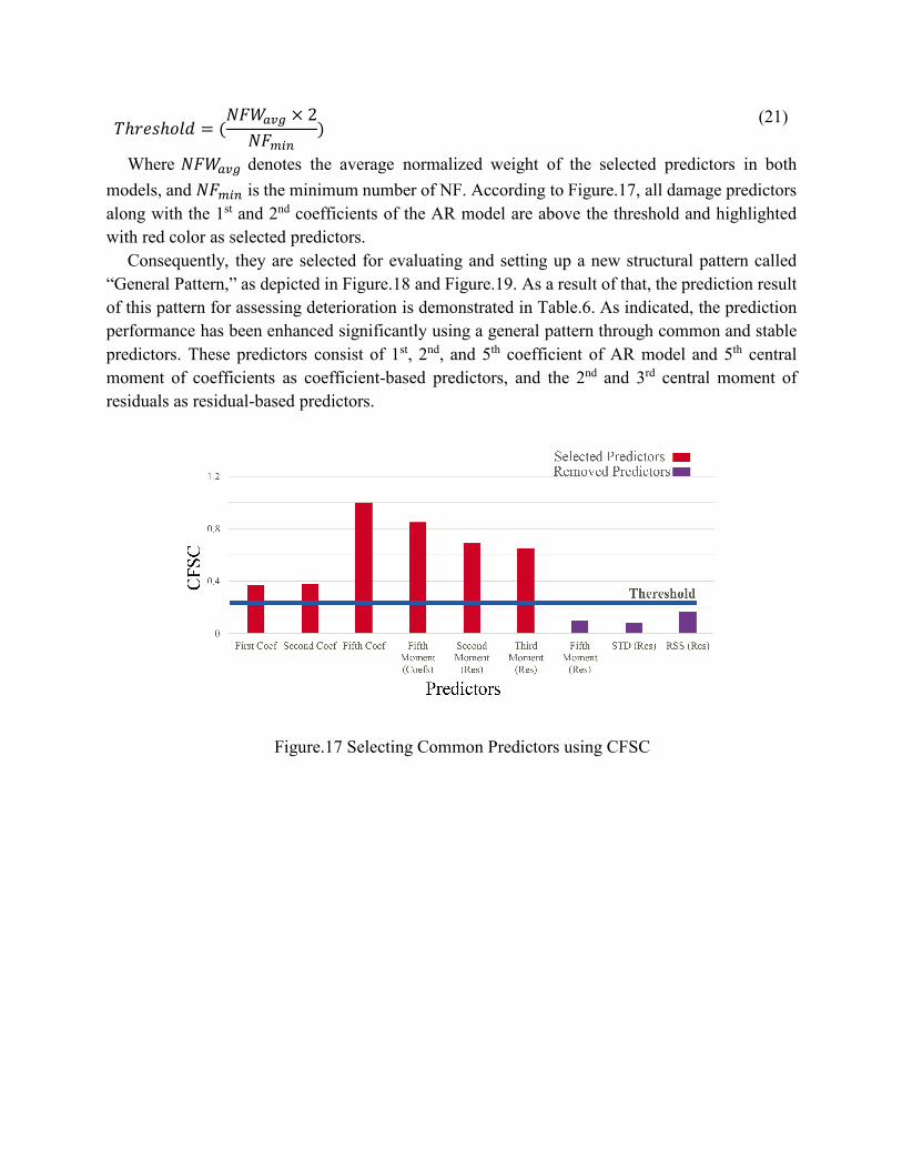
𝑇𝑇ℎ𝑟𝑟𝑒𝑒𝑠𝑠ℎ𝑐𝑐𝑜𝑜𝑑𝑑 = (𝑁𝑁𝐹𝐹𝑊𝑊𝑟𝑟𝑎𝑎𝐷𝐷 × 2𝑁𝑁𝐹𝐹𝑚𝑚𝑖𝑖𝑛𝑛

) (21)

Where 𝑁𝑁𝐹𝐹𝑊𝑊𝑟𝑟𝑎𝑎𝐷𝐷 denotes the average normalized weight of the selected predictors in both

models, and 𝑁𝑁𝐹𝐹𝑚𝑚𝑖𝑖𝑛𝑛 is the minimum number of NF. According to Figure.17, all damage predictors along with the 1st and 2nd coefficients of the AR model are above the threshold and highlighted with red color as selected predictors.

Consequently, they are selected for evaluating and setting up a new structural pattern called “General Pattern,” as depicted in Figure.18 and Figure.19. As a result of that, the prediction result of this pattern for assessing deterioration is demonstrated in Table.6. As indicated, the prediction performance has been enhanced significantly using a general pattern through common and stable predictors. These predictors consist of 1st, 2nd, and 5th coefficient of AR model and 5th central moment of coefficients as coefficient-based predictors, and the 2nd and 3rd central moment of residuals as residual-based predictors.

Figure.17 Selecting Common Predictors using CFSC

Figure.18 General Pattern of deterioration for the 1st story

Figure.19 General Pattern of damage for the story 1

Table.6 Accuracy of general pattern in classification Story Deterioration Damage

1 Scenario #1 83.3%

100.0% Scenario #2 91.7% Scenario#3 83.3%

2 Scenario#1 100.0%

100.0% Scenario#2 83.3% Scenario#3 100.0%

3 Scenario#1 100.0%

100.0% Scenario#2 100.0% Scenario#3 100.0%

In order to peruse the significance of pre-processing, two datasets of accelerations including

the first story of the first scenario in connection with the deterioration model and the first story in respect of the damage model are processed once more but in the following cases:

• Case A: data without pre-processing. • Case B: data without the whitening process.

As presented in Table.7, despite the significant influence of pre-processing on deterioration, it has a trifling impact on the result of the damage case. Hence, it reveals that stories have much higher correlations in the existence of minor changes due to deterioration rather than damage. Thus, ignoring the pre-processing step for the raw data leads to a significant drop of about 75% for deterioration assessment; however, regarding damage, this proportion reduction is less than 10%.

Table.7 The effect of the pre-processing stage on the accuracy of prediction

Model Case Accuracy

Deterioration A 25.0% B 33.3%

Damage A 92.9% B 96.4%

In this section, to study the effects of implementing more predictors, three cases of utilizing

different numbers of high-rank predictors are defined on the previous model as follows: • Case C: applying the first seven high-ranked predictors, • Case D: applying the first fifteen high-ranked predictors, • Case E: applying all of the predictors.

Concerning Table.8, the increase in the number of predictors leads to lower prediction efficiency. The result depicts a decline of 33.3% and 41.7% for the two first cases and more than 66.0% declination for the last case in terms of accuracy for the deterioration model. Besides,

turning to the damage model, it depicts a plunge of 25% for the first case and about 33% for the two other cases.

Eventually, to observe the effects of signal length, three distinct cases considered full, half and one-third of the length of original signals. Concerning Table.9, employing a shorter signal causes a drop in preciseness. However, the effect becomes negligible, even for implementing half of the initial data points for the damage model. Moreover, using even a shorter signal with a quarter length of the original signal leads to more significant errors in relation to deterioration detection rather than damage. Overall, it is evident that deterioration assessment is more sensitive in terms of signal length rather than damage detection.

Table.8 The effect of numbers of predictors on the result of the second stories

Model Case Accuracy

Deterioration C 66.7% D 58.3% E 33.3%

Damage C 75.0% D 66.7% E 66.7%

Table.9 The effect of length of signals on the result of the second stories Model Signal length ratio Accuracy

Deterioration 1 83.3%

1/2 66.7% 1/4 58.3%

Damage 1 100.0%

1/2 94.6% 1/4 62.5%

5. Conclusion In this study, a supervised assessment approach was introduced using enhanced AR time-series.

The method benefits from a new model order evaluation scheme called BMO in order to reduce the errors of time series estimation. A common set of predictors were selected from different types of statistical indices using a novel algorithm called BUFS, which creates a pattern of predictors outlining different structure states. The BUFS is able to select the features as predictors of a structural pattern in such a way that have not only the lowest correlations but also the highest impact in discriminating various types of datasets. The pattern was then utilized by a linear discriminant classifier in order to discriminate against the healthy states from the unknowns in two building models. Subsequently, the results indicated that the proposed approach is capable of

accurately identifying damage as well as deterioration, even in the existence of common measurement noise.

First, in the case of deterioration evaluation, the coefficient-based predictors seem more stable in all stories than the residual-based predictors. These stable predictors are the first and second coefficients of the AR model.

Second, concerning the damage case, it is evident that both coefficient- and residual-based predictors are consistent in all stories. Specifically, the most-practical predictors for damage detection are the fifth coefficient and central moments of coefficient as coefficient-based predictors, and the second and third central moments of residuals as residual-based predictors.

Eventually, a common set of predictors were selected using a new criterion called CFSC in order to develop a general pattern that can be used for detecting both damage and deterioration. This development is important because in most practical cases, there is no information about whether a structure is damaged or deteriorated. To this end, the general pattern including the first, second and fifth coefficients of the AR model, and the second and third central moments of residuals as common stable predictors that enhanced the performance of prediction for both models

Furthermore, the importance of pre-processing steps, including denoising, normalizing and whitening, should always be highlighted for deterioration assessment. It is also worth noting that the increase in the number of predictors has an inverse effect on the accuracy of prediction. Finally, there is an insignificant relation between signal length and the accuracy of classification for the damage assessment application, as evidenced by the case with a half number of data points; however, it has a significant impact on the case of deterioration detection.

Taken together, deterioration detection reveals more sensitivity in terms of signal length, number of predictors, and especially the pre-processing procedure including denoising and standardizing. Therefore, it requires more careful considerations in signal processing and interpretations. Moreover, the confident-based features are more reliable and stable in the case of damage and deterioration detection.

Competing Interest

The author(s) declared no potential conflicts of interest with respect to the research, authorship, and/or publication of this article.

6. References 1. Monavari B. SHM-based Structural Deterioration Assessment [PhD thesis]: Queensland

University of Technology 2019. 2. Sohn H, Farrar CR, Hemez FM, Czarnecki JJ. A review of structural health review of

structural health monitoring literature 1996-2001. Los Alamos National Laboratory; 2002. 3. Amezquita-Sanchez JP, Adeli H. Signal processing techniques for vibration-based health

monitoring of smart structures. Archives of Computational Methods in Engineering. 2016;23(1):1-15.

4. Gopalakrishnan S, Ruzzene M, Hanagud S. Computational techniques for structural health monitoring: Springer Science & Business Media; 2011.

5. Pawar PM, Ganguli R. Structural health monitoring using genetic fuzzy systems: Springer Science & Business Media; 2011.

6. Chatzi EN, Papadimitriou C. Identification Methods for Structural Health Monitoring: Springer; 2016.

7. Jaishi B, Ren W-X. Damage detection by finite element model updating using modal flexibility residual. Journal of sound and vibration. 2006;290(1):369-87.

8. Kim C-W, Kawatani M. Pseudo-static approach for damage identification of bridges based on coupling vibration with a moving vehicle. Structure and infrastructure engineering. 2008;4(5):371-9.

9. Moaveni B, Stavridis A, Lombaert G, Conte JP, Shing PB. Finite-element model updating for assessment of progressive damage in a 3-story infilled RC frame. Journal of Structural Engineering. 2012;139(10):1665-74.

10. Weber B, Paultre P. Damage identification in a truss tower by regularized model updating. Journal of structural engineering. 2009;136(3):307-16.

11. Bodeux J-B, Golinval J-C. Modal identification and damage detection using the data-driven stochastic subspace and ARMAV methods. Mechanical Systems and Signal Processing. 2003;17(1):83-9.

12. Deraemaeker A, Preumont A. Vibration based damage detection using large array sensors and spatial filters. Mechanical systems and signal processing. 2006;20(7):1615-30.

13. Kumar RP, Oshima T, Mikami S, Miyamori Y, Yamazaki T. Damage identification in a lightly reinforced concrete beam based on changes in the power spectral density. Structure and Infrastructure Engineering. 2012;8(8):715-27.

14. Ay AM, Wang Y. Structural damage identification based on self-fitting ARMAX model and multi-sensor data fusion. Structural Health Monitoring. 2014;13(4):445-60.

15. Lu Y, Gao F. A novel time-domain auto-regressive model for structural damage diagnosis. Journal of Sound and Vibration. 2005;283(3):1031-49.

16. Ivanovic SS, Trifunac MD, Todorovska M. Ambient vibration tests of structures-a review. ISET Journal of Earthquake Technology. 2000;37(4):165-97.

17. Lee J, Kim J, Yun C, Yi J, Shim J. Health-monitoring method for bridges under ordinary traffic loadings. Journal of Sound and Vibration. 2002;257(2):247-64.

18. Lee JJ, Yun CB. Damage diagnosis of steel girder bridges using ambient vibration data. Engineering Structures. 2006;28(6):912-25.

19. Siringoringo DM, Fujino Y. System identification of suspension bridge from ambient vibration response. Engineering Structures. 2008;30(2):462-77.

20. Zhang Q. Statistical damage identification for bridges using ambient vibration data. Computers & structures. 2007;85(7):476-85.

21. Siringoringo DM, Fujino Y. Experimental study of laser Doppler vibrometer and ambient vibration for vibration-based damage detection. Engineering Structures. 2006;28(13):1803-15.

22. Nguyen V, Dackermann U, Alamdari MM, Li J, Runcie P, editors. Model Updating for Loading Capacity Estimation of Concrete Structures using Ambient Vibration. International Symposium Non-Destructive Testing in Civil Engineering (NDT-CE); 2015.

23. Perez-Ramirez CA, Amezquita-Sanchez JP, Adeli H, Valtierra-Rodriguez M, Camarena-Martinez D, Romero-Troncoso RJ. New methodology for modal parameters identification of smart civil structures using ambient vibrations and synchrosqueezed wavelet transform. Engineering Applications of Artificial Intelligence. 2016;48:1-12.

24. Qiao L, Esmaeily A, editors. An overview of signal-based damage detection methods. Applied Mechanics and Materials; 2011: Trans Tech Publ.

25. Gonzalez C, Pleite J, Valdivia V, Sanz J, editors. An overview of the on line application of frequency response analysis (FRA). 2007 IEEE International Symposium on Industrial Electronics; 2007: IEEE.

26. Asgarian B, Aghaeidoost V, Shokrgozar HRJMS. Damage detection of jacket type offshore platforms using rate of signal energy using wavelet packet transform. 2016;45:1-21.

27. Su C, Jiang M, Liang J, Tian A, Sun L, Zhang F, et al. Damage identification in composites based on Hilbert Energy Spectrum and Lamb Wave Tomography algorithm. 2019.

28. Yang JN, Lei Y, Lin S, Huang NJJoem. Hilbert-Huang based approach for structural damage detection. 2004;130(1):85-95.

29. de Lautour OR, Omenzetter PJMS, Processing S. Damage classification and estimation in experimental structures using time series analysis and pattern recognition. 2010;24(5):1556-69.

30. Hu M-H, Tu S-T, Xuan F-ZJPE. Statistical Moments of ARMA (n, m) Model Residuals for Damage Detection. 2015;130:1622-41.

31. Farahani RV, Penumadu DJES. Damage identification of a full-scale five-girder bridge using time-series analysis of vibration data. 2016;115:129-39.

32. Lakshmi K, Rao ARM. Output-only damage localization technique using time series model. Sādhanā. 2018;43(9):147.

33. Monavari B, Chan TH, Nguyen A, Thambiratnam DPJIJoSS, Dynamics. Structural Deterioration Detection Using Enhanced Autoregressive Residuals. 2018;18(12):1850160.

34. Monavari B, Chan T, Nguyen A, Thambiratnam D, editors. Time-series coefficient-based deterioration detection algorithm. Proceedings of the 8th International Conference on Structural Health Monitoring of Intelligent Infrastructure (SHMII 2017); 2018: Curran Associates, Inc.

35. Nair KK, Kiremidjian AS, Law KH. Time series-based damage detection and localization algorithm with application to the ASCE benchmark structure. Journal of Sound and Vibration. 2006;291(1):349-68.

36. Vaseghi SV. Advanced digital signal processing and noise reduction: John Wiley & Sons; 2008.

37. Giurgiutiu V. Structural Health Monitoring with Piezoelectric Wafer Active Sensors 2nd Edition: Academic Press; 2014. 1024 p.

38. Smith SW. The Scientist and Engineer's Guide to Digital Signal Processing: California Technical Pub.; 1997.

39. Dorvash S, Yao R, Pakzad S, Okaly K, editors. Static and dynamic model validation and damage detection using wireless sensor networks. Proceedings of the 5th international conference on bridge maintenance, safety and management IABMAS2010, DM Frangopol, R Sause and CS Kusko Philadelphia, Pennsylvania, USA, Taylor & Francis Group, London; 2010.

40. Ren W-X, De Roeck G. Structural damage identification using modal data. II: Test verification. Journal of Structural Engineering. 2002;128(1):96-104.

41. Kessy A, Lewin A, Strimmer KJTAS. Optimal whitening and decorrelation. 2018;72(4):309-14.

42. Jonak K, Syta A, editors. Gearbox damage identification using Ensemble Empirical Decomposition method. MATEC Web of Conferences; 2019: EDP Sciences.

43. Jayaswal P, Aherwar AJTIJoME. Fault Detection and Diagnosis of Gear Transmission System via Vibration Analysis. 2011;4(3):26-43.

44. Cremona C, Cury A, Orcesi A. Supervised learning algorithms for damage detection and long term bridge monitoring. Measurement. 2012;4(2).

45. Robnik-Šikonja M, Kononenko IJMl. Theoretical and empirical analysis of ReliefF and RReliefF. 2003;53(1-2):23-69.

46. Lu S, Yu H, Zhang R, Wang X, editors. Damage identification method of carbon fiber reinforced polymer structure based on ReliefF and LSSVM. 2018 Chinese Control And Decision Conference (CCDC); 2018: IEEE.

47. Lu S, Jiang M, Wang X, Yu H, Su C. Damage degree prediction method of CFRP structure based on fiber Bragg grating and epsilon-support vector regression. Optik. 2019;180:244-53.

48. Babajanian Bisheh H, Ghodrati Amiri G, Nekooei M, Darvishan E. Damage detection of a cable-stayed bridge using feature extraction and selection methods. Structure and Infrastructure Engineering. 2019;15(9):1165-77.

49. Robnik-Šikonja M, Kononenko I, editors. An adaptation of Relief for attribute estimation in regression. Machine Learning: Proceedings of the Fourteenth International Conference (ICML’97); 1997.

50. Kononenko I, Šimec E, Robnik-Šikonja MJAI. Overcoming the myopia of inductive learning algorithms with RELIEFF. 1997;7(1):39-55.

51. Martinez-Luengo M, Kolios A, Wang L. Structural health monitoring of offshore wind turbines: A review through the Statistical Pattern Recognition Paradigm. Renewable and Sustainable Energy Reviews. 2016;64:91-105.

52. Nick W, Shelton J, Asamene K, Esterline AC, editors. A Study of Supervised Machine Learning Techniques for Structural Health Monitoring. MAICS; 2015.

53. Binkhonain M, Zhao L. A review of machine learning algorithms for identification and classification of non-functional requirements. Expert Systems with Applications. 2019.

54. Dey A. Machine learning algorithms: a review. International Journal of Computer Science and Information Technologies. 2016;7(3):1174-9.

55. de Lautour OR, Omenzetter P. Nearest neighbor and learning vector quantization classification for damage detection using time series analysis. Structural Control and Health Monitoring. 2010;17(6):614-31.

56. de Lautour OR, Omenzetter P. Damage classification and estimation in experimental structures using time series analysis and pattern recognition. Mechanical Systems and Signal Processing. 2010;24(5):1556-69.

57. Janeliukstis R, Rucevskis S, Chate A, editors. Classification-based Damage Localization in Composite Plate using Strain Field Data. Journal of Physics: Conference Series; 2018: IOP Publishing.

58. Silva Sd, Dias Júnior M, Lopes Junior V. Damage detection in a benchmark structure using AR-ARX models and statistical pattern recognition. Journal of the Brazilian Society of Mechanical Sciences and Engineering. 2007;29(2):174-84.

59. Wen C, Hung S, Huang C, Jan J. Unsupervised fuzzy neural networks for damage detection of structures. Structural Control and Health Monitoring: The Official Journal of the International Association for Structural Control and Monitoring and of the European Association for the Control of Structures. 2007;14(1):144-61.

60. Silva M, Santos A, Figueiredo E, Santos R, Sales C, Costa JC. A novel unsupervised approach based on a genetic algorithm for structural damage detection in bridges. Engineering Applications of Artificial Intelligence. 2016;52:168-80.

61. Behnia A, Chai HK, GhasemiGol M, Sepehrinezhad A, Mousa AA. Advanced damage detection technique by integration of unsupervised clustering into acoustic emission. Engineering Fracture Mechanics. 2019;210:212-27.

62. Farrar CR, Nix DA, Duffey TA, Cornwell PJ, Pardoen GC. Damage identification with linear discriminant operators. Los Alamos National Lab., NM (US); 1999.

63. Salehi H, Das S, Chakrabartty S, Biswas S, Burgueño R, editors. Structural assessment and damage identification algorithms using binary data. ASME 2015 conference on smart materials, adaptive structures and intelligent systems; 2015: American Society of Mechanical Engineers Digital Collection.

64. Nardi D, Lampani L, Pasquali M, Gaudenzi P. Detection of low-velocity impact-induced delaminations in composite laminates using Auto-Regressive models. Composite Structures. 2016;151:108-13.

65. Jiménez AA, Márquez FPG, Moraleda VB, Muñoz CQG. Linear and nonlinear features and machine learning for wind turbine blade ice detection and diagnosis. Renewable energy. 2019;132:1034-48.

66. Izenman AJ. Multivariate regression. Modern Multivariate Statistical Techniques: Springer; 2013. p. 159-94.

67. Xanthopoulos P, Pardalos PM, Trafalis TB. Robust data mining: Springer Science & Business Media; 2012.

68. Liu L, Özsu MT. Encyclopedia of database systems: Springer New York, NY, USA:; 2009. 69. Burkov A. The Hundred-Page Machine Learning Book: Andriy Burkov; 2019. 70. Reinhorn AM, Roh H, Sivaselvan MV, Kunnath SK, Valles R, Madan A, et al. IDARC2D

Version 7.0: A Program for the Inelastic Damage Analysis of Structues. 2006. 71. Los Alamos National Laboratory [Available from: https://www.lanl.gov/. 72. Figueiredo E, Park G, Figueiras J, Farrar C, Worden KJLANL, Los Alamos, NM, Report

No. LA-14393. Structural health monitoring algorithm comparisons using standard data sets. 2009.

7. Appendix

Table A1. Statistical Indices (DIs) Index Definition

AR coefficients 𝐶𝐶1, 𝐶𝐶2,…

Central moments (orders 2 to 8) 𝑅𝑅𝑘𝑘 = 𝐸𝐸[(𝑠𝑠 − 𝜇𝜇)𝑘𝑘]

Range 𝑅𝑅𝑛𝑛 = max(s) − min(s)

Interquartile range 𝐼𝐼𝐼𝐼𝑅𝑅 = 𝐼𝐼3(𝑠𝑠) − 𝐼𝐼1(𝑠𝑠)

Median absolute deviation (MAD) 𝑅𝑅𝑀𝑀𝑀𝑀 = 𝑚𝑚𝑒𝑒𝑑𝑑𝑖𝑖𝑟𝑟𝑛𝑛(|𝑠𝑠 − �̃�𝑠|)

Root-mean-square (RMS) 𝑅𝑅𝑅𝑅𝑅𝑅 = �1𝑁𝑁�|𝑠𝑠𝑛𝑛|2𝑁𝑁

𝑛𝑛=1

Standard deviation (STD) 𝑅𝑅𝑇𝑇𝑀𝑀 = �1

𝑁𝑁 − 1�|𝑠𝑠𝑛𝑛 − 𝜇𝜇|2𝑁𝑁

𝑛𝑛=1

Skewness 𝑅𝑅𝑟𝑟 =𝐸𝐸(s − μ)3

𝜎𝜎3

Kurtosis 𝐾𝐾 =𝐸𝐸(s − μ)4

𝜎𝜎4

Impulse Factor 𝐼𝐼𝐹𝐹 =

max (s)1𝑁𝑁∑ |𝑠𝑠𝑛𝑛|𝑁𝑁

𝑛𝑛=1

Crest factor 𝐶𝐶𝐹𝐹 =

𝑚𝑚𝑟𝑟𝑥𝑥 (s)RMS (𝑠𝑠)

Energy 𝐸𝐸 = �|𝑠𝑠𝑛𝑛2|𝑁𝑁

𝑛𝑛=1

FM4 factor 𝐹𝐹𝑅𝑅4 = �4𝐷𝐷ℎ𝑅𝑅𝑐𝑐𝑚𝑚𝑒𝑒𝑛𝑛𝑡𝑡

𝑐𝑐𝑟𝑟𝑟𝑟2

𝑁𝑁

𝑛𝑛=1

The root-sum-of-squares (RSS) level 𝑅𝑅𝑅𝑅𝑅𝑅 = ��|𝑠𝑠𝑛𝑛2|𝑁𝑁

𝑛𝑛=1

8. Nomenclature

Symbol Description 𝑵𝑵 Numbers of samples 𝝁𝝁 Sample mean 𝑬𝑬 The expectation value of samples 𝝈𝝈 Standard deviation 𝒗𝒗𝒗𝒗𝒗𝒗 Variance of samples