LU TP 14-13June 4, 2014

SUPERSYMMETRY IN QUANTUM MECHANICS

Simon Kuberski

Department of Astronomy and Theoretical Physics, Lund University

Bachelor thesis supervised by Johan Bijnens

Abstract

This thesis gives an introduction to the basic formalism of one-dimensional supersymmetricquantum mechanics. The factorization of a Hamiltonian is used to create a supersymmetricpartner Hamiltonian. The connections between the energy spectra and wave functions ofthese partner Hamiltonians are deduced and examined for the case of broken and unbrokensupersymmetry. An extension to hierarchies of Hamiltonians is made and used to describeshape invariant potentials.The formalism is used to solve some textbook examples like the infinite square well andthe harmonic oscillator potential in a new way and to determine the wave functions andenergy levels of the hydrogen atom in a nonrelativistic and a relativistic treatment.A two-dimensional extension of the formalism is introduced and applied to find a way tosolve the eigenvalue problem for a matrix Pauli Hamiltonian through its scalar partnerHamiltonians. The two-dimensional formalism is further used to examine a chain of two-dimensional real singular Morse potentials and to determine the wave functions and energyspectra based on the solution of the one-dimensional Morse potential.

1

Popularvetenskapligt sammanfattning

A quantum mechanics course belongs to the main parts of undergraduate physics stud-ies and the content is necessary as a basis in all fields of modern physics. However thetreatment of supersymmetric quantum mechanics as described in this thesis does not ingeneral belong to the curriculum although it offers different and sometimes easier solutionsto problems that are solved in a quantum mechanics course.The basis of supersymmetric quantum mechanics was set in theoretical particle physics.Many of the properties of the universe can today be described by the standard model ofparticle physics that includes the known particles and forces that build up our universe.The study of their properties is a very active field and news from the Large Hadron Col-lider at CERN like the confirmation of the existence of the Higgs particle cause a lot ofinterest. Despite its great success, the standard model is not able to describe all processesin the world of particle physics and theoretical physicists try to extend the model to beable to predict and explain these processes. A theory that arose was supersymmetry. Itstates that every one of the basic particles, which can be distinguished between fermionsand bosons, has a partner with the exact mass that is of the other kind. This model allowsit to explain some of the processes that are not included in the standard model. Unfor-tunately the concept has not been confirmed experimentally, today none of the predictedsuperparticles have been observed which would have been the case if they had the samemass as their already known counterparts. The only explanation that can save the conceptof supersymmetry is a spontaneous symmetry breaking. The search for possible breakingmechanisms and their mathematical description led to the development of supersymmetricquantum mechanics.The formalism of this concept is used in this thesis to solve well-known problems in quan-tum mechanics in a new and elegant way and to find solutions for problems that cannot behandled with other methods. This thesis starts with presenting the easiest application, theone-dimensional treatment. The formalism is introduced and its use is shown by solvingsome examples. The second part of the thesis handles two-dimensional problems whichare the first step to a general higher-dimensional description of supersymmetric quantummechanics. For example it is shown that it is possible to solve certain two-dimensionalproblems just by knowing the solution of a simpler one-dimensional problem and the for-malism of supersymmetric quantum mechanics.

2

Contents

1 Introduction 5

2 Formalism of Supersymmetric Quantum Mechanics 62.1 Factorization of the One Dimensional Hamiltonian . . . . . . . . . . . . . 62.2 Partner Hamiltonians and Potentials . . . . . . . . . . . . . . . . . . . . . 72.3 Broken Supersymmetry . . . . . . . . . . . . . . . . . . . . . . . . . . . . . 92.4 Hierarchy of Hamiltonians . . . . . . . . . . . . . . . . . . . . . . . . . . . 102.5 Shape Invariant Potentials . . . . . . . . . . . . . . . . . . . . . . . . . . . 12

3 Examples 143.1 Infinite Square Well . . . . . . . . . . . . . . . . . . . . . . . . . . . . . . . 143.2 The Harmonic Oscillator . . . . . . . . . . . . . . . . . . . . . . . . . . . . 163.3 The Nonrelativistic Hydrogen Atom . . . . . . . . . . . . . . . . . . . . . . 183.4 The Dirac Equation . . . . . . . . . . . . . . . . . . . . . . . . . . . . . . . 21

4 Two-Dimensional SUSY QM 254.1 The Pauli Hamiltonian in Two Dimensions . . . . . . . . . . . . . . . . . . 274.2 Exact Solution of a Two-Dimensional Model with Real Spectrum . . . . . 29

4.2.1 The Two-Dimensional Real Singular Morse Potential . . . . . . . . 294.2.2 Shape Invariance of the Two-Dimensional Morse Model . . . . . . . 35

5 Conclusions 38

A Derivations 39A.1 Connection between the Wave Functions in the Two-Dimensional Morse

Potential . . . . . . . . . . . . . . . . . . . . . . . . . . . . . . . . . . . . 39A.2 The Operator T . . . . . . . . . . . . . . . . . . . . . . . . . . . . . . . . 40A.3 Zero Modes of Q†(ak) . . . . . . . . . . . . . . . . . . . . . . . . . . . . . 41

3

List of Figures

1 Scheme of the energy spectra of two supersymmetric partner Hamiltoniansand their connection via the operators A and A†. . . . . . . . . . . . . . . 8

2 Comparison between the eigenfunctions and energy levels of the infinitesquare well potential V (1) and its partner potential V (2). . . . . . . . . . . 15

3 Shape invariant harmonic oscillator potentials V (n) for n = 1,2,3,4 and thefirst superpotential W (r) for l = 2. . . . . . . . . . . . . . . . . . . . . . . 17

4 Eigenfunctions of the harmonic oscillator ψ(1)n (r,l) for n = 0,1,2 at their

energy levels E(1)n and the corresponding potential V (1)(r,l) for l = 1. . . . 18

5 The effective radial Coulomb potential V (1)(r), the partner potential V (2)(r)and the superpotential W (r) for l = 1. . . . . . . . . . . . . . . . . . . . . 20

6 One-dimensional Morse potential and the two-dimensional model of a Morsepotential. . . . . . . . . . . . . . . . . . . . . . . . . . . . . . . . . . . . . 31

4

1 Introduction

Supersymmetry (SUSY) is a concept that was developed in particle physics. The advantageof this model is its ability to give answers to questions that cannot be explained withthe standard model of particle physics. It postulates a symmetry between half-integerspin fermions and integer spin bosons where each boson and fermion is supposed to havea superpartner with the same mass. This symmetry has not been not observed yet innature so it has to be spontaneously broken. In 1981 Edward Witten proposed a simplequantum mechanical model to study a possible breaking mechanism for SUSY in his articleDynamical breaking of supersymmetry [1] and the new idea of supersymmetric quantummechanics has grown to a research field on its own.

This thesis gives an insight into the basic formalism of supersymmetric quantum me-chanics and shows the application of the formalism for some exemplary problems. Basedon the work in [2], [3], [4], [5] and [6] it starts with the factorization of the one-dimensionalHamiltonian as a first step to the creation of partner Hamiltonians and potentials. Theproperties of these partner potentials are evaluated and discussed and the special case ofbroken supersymmetry is described. The next step is the extension of the formalism fortwo partner Hamiltonians to a whole hierarchy of Hamiltonians which are connected viasupersymmetry. This allows to introduce the concept of shape invariant potentials (SIP)which can be used to determine the properties of all members of a chain of Hamiltoniansand to algebraically solve their spectrum just based on the properties of the first one .

The possibility of constructing a partner potential with an energy spectrum that isnearly identical to the original one is first applied to the well-known infinite square well.The wave functions and energy levels of this standard text book example are used to deter-mine the properties of the new potential. As a next step the harmonic oscillator potentialis used to present the application of the SIP-formalism. A sequence of partner potentialsis constructed and the energy levels of all potentials are determined.Afterwards the properties of the radial Coulomb potential in a hydrogen atom are de-termined. In the first case this is done in a nonrelativistic manner and the formalismof supersymmetric quantum mechanics allows the determination of the energy levels andwave functions in accordance with the solutions which are obtained via the normal text-book calculations. The next step is the relativistic treatment of the same potential. Thisis shown based on the work done in [3], [7] and [8]. The problem can be treated just likethe far simpler potentials and is a good example for the possibility to use the introducedformalism to find a simpler solution than the ones in textbook examples.

In the last part of the thesis a higher dimensional treatment of supersymmetric quan-tum mechanics as described in [9] is introduced. The extension of the formalism to twodimensions is shown and the relations between the new partner Hamiltonians are derived.An analogy of the matrix Hamiltonian that appears in the two-dimensional treatment canbe found in the Pauli Hamiltonian for the movement of a fermion in two dimensions. It isshown that the scalar partner potentials can be used to solve the eigenvalue problem forthe Pauli Hamiltonian. The formalism is also used to handle a two-dimensional model of aMorse potential which is introduced in [10] and [11]. This model contains two partner po-

5

tentials that depend on two variables. The solution of one of the potentials via separationof variables allows the determination of the wave functions and energy levels of the partnerpotential. Afterwards the potentials are examined for shape invariance and this propertyis used to determine the wave functions and energy levels of a whole chain of Hamiltonians.

2 Formalism of Supersymmetric Quantum Mechanics

2.1 Factorization of the One Dimensional Hamiltonian

The exact solution of one-dimensional potential problems is a basic task in quantum me-chanics. The eigenvalue of the Hamiltonian H(1) acting on a known ground state wavefunction ψ0(x) is the ground state energy E

(1)0 . If ψ0(x) is assumed to be nodeless and

normalizable and if E(1)0 is shifted to zero, applying of H(1) yields

H(1)ψ0(x) = − ~2

2m

d2ψ0

dx2+ V (1)(x)ψ0(x) = 0, (2.1)

from which it is possible to reconstruct the potential V (1)(x):

V (1)(x) =~2

2m

ψ′′0(x)

ψ0(x). (2.2)

The Hamiltonian H(1) can be factorized into two operators

H(1) = A†A (2.3)

where

A =~√2m

d

dx+W (x) and A† = − ~√

2m

d

dx+W (x), (2.4)

with the superpotential W (x) which is connected with the potential V (1)(x). The relationcan be found by comparing the two different forms of H(1):

H(1)ψ(x) = A†Aψ(x) =

(− ~2

2m

d2

dx2− ~√

2mW ′(x) +W (x)2

)ψ0(x) (2.5)

=

(− ~2

2m

d2

dx2+ V (1)(x)

)ψ(x)

The resulting differential equation

V (1)(x) = W 2(x)− ~√2m

W ′(x). (2.6)

6

is known as the Ricatti equation. The general solution of this equation can be found whena special solution is known. Knowing that H(1)ψ0 = A†Aψ0 = 0 is fulfilled when Aψ0 = 0,leads with (2.4) to a solution for W (x):

W (x) =−~√2m

ψ′0(x)

ψ0(x)=−~√2m

d(lnψ0(x))

dx. (2.7)

The ground state wave function ψ0 can be denoted as zero mode of A. The differentialequation (2.7) can be used to calculate ψ0 with a known superpotential

ψ(1)0 (x) = N exp

(−√

2m

~

∫ x

W (x′)dx′

), (2.8)

where N is a normalization constant.

2.2 Partner Hamiltonians and Potentials

Exchanging the order of the two operators in the factorized Hamiltonian generates thesupersymmetric partner Hamiltonian

H(2) = AA† = − ~2

2m

d2

dx2+W (x)2 +

~√2m

W ′(x)

≡ − ~2

2m

d2

dx2+ V (2)(x) (2.9)

with the partner potential

V (2)(x) = W (x)2 +~√2m

W ′(x). (2.10)

These partner Hamiltonians are related not only by the superpotential but also by theirenergy eigenvalues and wave functions. The energy eigenvalues of the Hamiltonians H(1)

and H(2) are both positive-semidefinite (E(1,2)n ≥ 0). Starting with n > 0 the Schrodinger

equation for H(1)

H(1)ψ(1)n = A†Aψ(1)

n = E(1)n ψ(1)

n (2.11)

helps to find an energy eigenvalue equation for H(2) which connects the eigenvalues of bothHamiltonians:

H(2)(Aψ(1)n ) = AA†Aψ(1)

n = E(1)n (Aψ(1)

n ). (2.12)

The same can be done for the Schrodinger equation for H(2)

H(2)ψ(2)n = AA†ψ(2)

n = E(2)n ψ(2)

n (2.13)

7

implies

H(1)(A†ψ(2)n ) = A†AA†ψ(2)

n = E(2)n (A†ψ(2)

n ) (2.14)

Equations (2.12) and (2.14) show that A†ψ(2)n is an eigenstate of H(1) and Aψ

(1)n is an

eigenstate of H(2) respectively. Using this result and equations (2.11)-(2.14) it is now

possible to include the case n = 0 with E(1)n = 0 and formulate the relations between the

two Hamiltonians for n = 0,1,2,...

E(2)n = E

(1)n+1, E

(1)0 = 0, (2.15)

ψ(2)n =

(E

(1)n+1

)− 12Aψ

(1)n+1, (2.16)

ψ(1)n+1 =

(E(2)n

)− 12 A†ψ(2)

n , (2.17)

where the normalization constants can be gained from the norm of the eigenfunctions, forexample

||Aψ(1)n+1||2 = 〈ψ(1)

n+1|A†A|ψ(1)n+1〉 = 〈ψ(1)

n+1|H(1)|ψ(1)n+1〉 = E

(1)n+1. (2.18)

The relations

AH(1) = AA†A = H(2)A and H(1)A† = A†AA† = A†H(2) (2.19)

which are used for the calculations of the eigenvalues above are called intertwining re-lations. This way of expressing the connection between the Hamiltonians is used in thetwo-dimensional treatment which is described later.

Equation (2.15) shows that the energy spectra of both Hamiltonians are nearly exactlythe same, the only difference is an additional ground state of H(1). The operators A andA† are used to switch between the two systems. A maps the eigenfunction of H(1) tothe partner system and destroys one node of the eigenfunction. Vice versa A† maps aneigenfunction of H(2) to the system of H(1) and creates an additional node. This makes itpossible to determine all eigenfunctions and energy eigenvalues of the second system whenthe first system is known. This works vice versa except for the ground state wave functionof H(1). The energy spectra and the mapping are illustrated in figure 1

A†

A

H(2)H(1)

E

Figure 1: Scheme of the energy spectra of two supersymmetric partner Hamiltonians andtheir connection via the operators A and A†.

8

This coincidence of the spectra has its origin in the algebra of supersymmetry. TheHamiltonians and the factorization operators can be presented as elements of matrix 2× 2operators, the superhamiltonian H and the supercharges Q±

H =

(H(1) 0

0 H(2)

)Q =

(0 0A 0

)Q† =

(0 A†

0 0

). (2.20)

In this form the elements describe the supersymmetric algebra [2] and obey the commuta-tion and anticommutation relations

[H,Q] = [H,Q†] = 0, {Q,Q†} = H, {Q,Q} = {Q†,Q†} = 0. (2.21)

As described in the introduction supersymmetry creates a connection between bosons andfermions or bosonic and fermionic states and the algebra mirrors this. The two Hamilto-nians in the superhamiltonian are the Hamiltonians of the bosonic state and the fermionicstates respectively. The total wave function

ψn =

(ψ

(1)n

ψ(2)n

);

ψ(1)n : bosonic

ψ(2)n : fermionic

(2.22)

contains the wave functions of both states. The supercharges are the symmetry operatorswhich change bosonic in fermionic states and vice versa

Q|boson〉 ∝ |fermion〉 and Q†|fermion〉 ∝ |boson〉. (2.23)

Apparently the left spectrum in figure 1 belongs to the bosonics states and the right oneto the fermionic. The ground state is bosonic.

2.3 Broken Supersymmetry

Although SUSY is considered to be a good explanation for many unsolved problems in thestandard model, it has not been observed in nature. A possible explanation is that SUSYis spontaneously broken. This symmetry breaking can also be described in supersymmetricquantum mechanics.

In the former sections it was assumed that the ground state energy E(1)0 is zero. This

assumption leads to the equation for the normalizable ground state wave function ψ(1)0 in

(2.8) and the relations between the eigenfunctions of the partner Hamiltonians in (2.16)

and (2.17). The normalization of ψ(1)0 determines some properties of the superpotential;

the exponential function has to vanish at the boundaries, the exponent has to go to minusinfinity. This means that the integral of the superpotential has to converge to infinity forx→ ±∞, so ∫ 0

−∞W (x′)dx′ =∞ and

∫ ∞0

W (x′)dx′ =∞. (2.24)

9

Therefore W (x) has to converge to infinity for large positive values of x and to convergeto minus infinity for large negative values of x. If these criteria are fulfilled SUSY isunbroken.If the properties of the two partner Hamiltonians are just switched, which means thatE

(2)0 = 0, E

(1)0 6= 0 and ψ

(2)0 (x) is normalizable, SUSY is unbroken, too. This case does

not have to be considered specially because exchanging the definitions of H(1) and H(2)

restores the former case.If neither E

(1)0 nor E

(2)0 are zero, the application of the ladder operators A and A† to

the ground state wave functions does not annihilate them. This implies that the operatorsdo not destroy nodes. In this case the energy spectra of both partner potentials are exactlythe same and all energy eigenvalues are positive

E(1)n = E(2)

n > 0. (2.25)

The operators A and A† still switch between the eigenfunctions on the same energy levels

ψ(2)n =

(E(1)n

)− 12 Aψ(1)

n and ψ(1)n =

(E(2)n

)− 12 A†ψ(2)

n . (2.26)

In this case SUSY is broken.This breaking can also be described with the algebra of supersymmetry. In general the

action of a symmetry operator on one state gives a symmetric one. The exception fromthis is the ground state which is unique. So the action of a symmetry operator on theground state has to result in zero, the symmetry operators must annihilate the vacuum.Because of {Q,Q†} = QQ† + Q†Q = H from equation (2.21), the ground state energy aseigenvalue of H has to be zero. If the ground state energy in nonzero and the ground stateis not unique anymore supersymmetry is broken.

2.4 Hierarchy of Hamiltonians

The previous sections show that it is possible to factorize a Hamiltonian H(1) into twooperators A and A† that are dependent on the superpotential W (x). It is further shownthat these operators can be used to create a new Hamiltonian H(2). The introduction of anew superpotential W2(x) allows a refactorization of H(2) in two new operators A2 and A†2.The partner Hamiltonian that can be created by the commutation of A2 and A†2 is calledH(3) and similar to the calculations above it is possible to determine the energy levels andground state wave functions of this new Hamiltonian. H(3) has the same energy spectrumas H(2) except for the ground state E

(2)0 . The repeated application of this procedure leads

to the creation of a chain of Hamiltonians, each with an energy level less than the previousone. The number of Hamiltonians is limited by the number of bound states in the firstpotential. The knowledge of the wave functions and the energy levels of H(1) makes itpossible to calculate the energy spectrum and the wave functions of all Hamiltonians.

Although the previous treatment of the first Hamiltonian assumed the ground state tobe zero, this is not in general the case so the Hamiltonian H(1) is rewritten as

H(1) = A†1A1 + E(1)0 = − ~2

2m

d2

dx2+ V (1)(x), (2.27)

10

with the rewritten potential

V (1) = W1(x)2 − ~√2m

W ′1(x) + E

(1)0 , (2.28)

where the operators A and A† from section 2.1 are written with the index 1 for clarity andE

(1)0 is the ground state energy of H(1).

Similar to the steps in section 2.2 the partner Hamiltonian H(2) can be calculated byan exchange of the operators

H(2) = A1A†1 + E

(1)0 = − ~2

2m

d2

dx2+ V (2)(x) (2.29)

with the potential

V (2) = W1(x)2 +~√2m

W ′1(x) + E

(1)0

= V (1)(x) +2~√2m

W ′1(x) = V (1)(x)− 2~√

2m

d2

dx2ln(ψ

(1)0

). (2.30)

Similar to the former calculations the associated energy levels and wave functions arecalculated by

E(2)n = E

(1)n+1, (2.31)

ψ(2)n =

(E

(1)n+1 − E

(1)0

)− 12A1ψ

(1)n+1. (2.32)

The ground state energy of H(2) is E(2)0 = E

(1)1 . The Hamiltonian can be refactorized as

H(1) before,

H(2) = A1A†1 + E

(1)0 = A†2A2 + E

(2)0 = A†2A2 + E

(1)1 (2.33)

with the new factorization operators similar to the former calculations

A2 =~√2m

d

dx+W2(x), A†2 = − ~√

2m

d

dx+W2(x) (2.34)

and the new superpotential

W2(x) = − ~√2m

ψ′(2)0 (x)

ψ(2)0 (x)

= − ~√2m

d

dxln(ψ

(2)0

). (2.35)

It is now possible to obtain the third Hamiltonian in the same manner

H(3) = A2A†2 + E

(1)1 = − ~2

2m

d2

dx2+ V (3)(x) (2.36)

11

with the potential

V (3)(x) = W2(x)2 +~√2m

W ′2(x) + E

(1)1

= V (2)(x)− 2~√2m

d2

dx2ln(ψ

(2)0

)= V (1)(x)− 2~√

2m

d2

dx2ln(ψ

(1)0 ψ

(2)0

)(2.37)

and the corresponding energy levels and wave functions

E(3)n = E

(2)n+1 = E

(1)n+2 (2.38)

ψ(3)n =

(E

(2)n+1 − E

(2)0

)− 12A2ψ

(2)n+1

=(E

(1)n+2 − E

(1)1

)− 12(E

(1)n+2 − E

(1)0

)− 12A2A1ψ

(1)n+1. (2.39)

It can be seen that it is possible to express the energy levels and wave functions in termsof the system of the first Hamiltonian. This allows to create a whole chain of Hamiltonianslike it was stated in the introduction of this section. Equation (2.38) implies that everyHamiltonian has the same energy spectrum as the former one except for the ground state.The cut off of the ground states leads to the limitation of Hamiltonian numbers based onthe number of energy levels in the first potential. Figure 1 could be increased by additionalenergy ladders, which are connected by the operators An and A†n.The procedure of creating a chain of Hamiltonians is used in the treatment of ShapeInvariant Potentials (SIP).

2.5 Shape Invariant Potentials

The analytical determination of energy eigenvalues and eigenfunctions is possible for anumber of potentials and a common property of these potentials is called shape invariance.If two supersymmetric partner potentials are shape invariant, they have a similar shapeand differ only in the set of parameters they are defined in and a remainder. This can beexpressed with

V (2)(x,a1) = V (1)(x,a2) +R(a1) (2.40)

where a1 is a set of parameters and a2 is a different set of parameters that can be expressedas a function f of a1; a2 = f(a1). The remainder R(a1) is independent of x.

In order to study the properties of SIP, a chain of Hamiltonians can be constructed inthe way it is shown in the previous section. Starting with a Hamiltonian H(1) with E

(1)0 = 0

and

H(1) = − ~2

2m

d2

dx2+ V (1)(x,a1), (2.41)

12

the chain of Hamiltonians H(s) with s = 1,2,3,... contains as many members as there arebound states in V (1)(x,a1). A repeated use of the shape invariance condition (2.40) allowsa comparison between two sequent shape invariant Hamiltonians H(s) and H(s+1)

H(s) = − ~2

2m

d2

dx2+ V (1)(x,as) +

s−1∑k=1

R(ak), (2.42)

H(s+1) = − ~2

2m

d2

dx2+ V (1)(x,as+1) +

s∑k=1

R(ak)

(2.40)= − ~2

2m

d2

dx2+ V (2)(x,as) +

s−1∑k=1

R(ak) (2.43)

where ak = f (k)(a1) means that f is applied k times. The comparison shows that theHamiltonians are according to (2.40) partner Hamiltonians and therefore have identicalenergy levels except for the ground state of H(s) which is

E(s)0 =

s−1∑k=1

R(ak) (2.44)

because E(1)0 = 0.

It is possible to go back from H(s) to H(1) where an energy level is added for every stepuntil the level E = 0 is reached. Thus the complete energy spectrum of H(1) is describedby

E(1)n (a1) =

n∑k=1

R(ak); E(1)0 = 0. (2.45)

Because the Operators An and A†n link the eigenfunctions at the same energy levelsfor different partner Hamiltonians, they can be used to determine the bound state wavefunctions ψ

(1)n (x,a1) for a shape invariant potential based on the known ground state wave

function ψ(1)0 (x,a1). Equation (2.42) shows that each Hamiltonian depends on the potential

V (1)(x,a) and a set of parameters as. Thus the ground state wave function of H(s) is

ψ(1)0 (x,as), which is a consequence of the shape invariance condition (2.40) and

ψ(s)n (x,a1) = ψ(1)

n (x,as). (2.46)

The relation between wave functions of the two partner Hamiltonians at the same energylevel (2.17) can now be used to express the first excited wave function of a HamiltonianH(s)

ψ(1)1 (x,as) ∝ A†(x,as)ψ

(2)0 (x,as) = A†(x,as)ψ

(1)0 (x,as+1). (2.47)

13

Repeating this step makes it possible to determine the n’th unnormalized wave functionof the first Hamiltonian H(1)

ψ(1)n (x,a1) ∝ A†(x,a1)ψ

(1)n−1(x,a2), (2.48)

ψ(1)n (x,a1) ∝ A†(x,a1)A

†(x,a2) . . . A†(x,an)ψ

(1)0 (x,an+1). (2.49)

The explicit relation (2.17) leads to the formula

ψ(1)n (x,a1) =

(E(1)n

)− 12 A†(x,a1)ψ

(1)n−1(x,a2) (2.50)

and the possibility to determine all wave functions and energy levels of Hamiltonians obey-ing the SIP condition just by knowing the first ground state wave function the remainderR(a) and the relation between two subsequent sets of parameters f(a).

Hence the property of shape invariance simplifies the treatment of partner potentialsand their wave functions considerably. Table I of [4] shows all shape invariant potentialsthat were known at the time of its publication and their properties.

3 Examples

3.1 Infinite Square Well

Calculating the energy levels and wave functions of the bound states in a square well ofinfinite depth is a basic task in a quantum mechanics lecture. The formalism of supersym-metric quantum mechanics makes it possible to use the well-known solutions to create asupersymmetric partner potential with the same energy levels and its eigenfunctions.

Starting with an symmetric infinite square well with the potential

V (x) =

{0 if |x| ≤ L

2

∞ else(3.1)

the Schrodinger equation

Hψn(x) =

(− ~2

2m

d2

dx2+ V (x)

)ψn(x) = Enψn(x) (3.2)

reduces to

ψ′′n(x) = −2m

~2Enψn(x) (3.3)

for |x| ≤ L2

with En ≥ 0. This symmetrical potential has symmetric ψ(s)n and antisymmetric

ψ(a)n wave functions as eigenfunctions. With n equivalent to the number of nodes the

eigenfunction can be written as

ψn(x) =

ψ(s)n (x) =

√2L

cos(

(n+1)πL

x)

for n = 0,2,4,...

ψ(a)n (x) =

√2L

sin(

(n+1)πL

x)

for n = 1,3,5,...(3.4)

14

and the energy levels are

En =π2~2

2mL2(n+ 1)2. (3.5)

The factorization of the Hamiltonian requires the ground state energy to be zero, whichleads to a necessary shift of the potential and the connected energy levels

V (1)(x) = V (x)− E0 and E(1)n =

π2~2

2mL2n(n+ 2). (3.6)

The superpotential W (x) is calculated with the ground state wave function ψ0(x) andequation (2.7)

W (x) =~π√2mL

tan(π

Lx) (3.7)

and is used to determine the partner potential V (2) with equation (2.10)

V (2) =~2π2

2mL2

(1 + 2 tan2

(πLx))

, (3.8)

E(2)n =

π2~2

2mL2(n+ 1)(n+ 3) (3.9)

and its energy levels according to the relations given in (2.15). The eigenfunctions are

-L/2 L/2 0

x

(a) Squared eigenfunctions ψ(1)n

in the shifted infinite square wellpotential V (1).

-L/2 L/2 0

x

(b) Squared eigenfunctions ψ(2)n

in the supersymmetric partnerpotential V (2).

Figure 2: Comparison between the eigenfunctions and energy levels of the infinite squarewell potential V (1) and its partner potential V (2).

15

determined with the definition of A in (2.4) and equation (2.16)

ψ(2)n =

(E

(1)n+1

)− 12Aψ

(1)n+1

=

(

2L(n+1)(n+3)

) 12(

(n+ 2) cos(

(n+2)πL

x)

+ tan(πLx)

sin(

(n+2)πL

x))

for n even(2

L(n+1)(n+3)

) 12(−(n+ 2) sin

((n+2)πL

x)

+ tan(πLx)

cos(

(n+2)πL

x))

for n odd.

(3.10)

The squared eigenfunctions at their corresponding energy levels in the two potentials areshown in figure 2. The comparison between the figures 2(a) and 2(b) shows that theconclusions of section 2.2 fit to the calculated functions and energy levels. As expected,V (2) has the exact same energy levels as V (1) except for the missing ground state E

(1)0 .

Switching from ψ(1)n+1 to ψ

(2)n with the operator A destroys one node.

3.2 The Harmonic Oscillator

One of the known shape invariant potentials is the three-dimensional oscillator potential.The treatment of the radial equation is a good example for the use of the properties ofshape invariant potentials. The superpotential can be taken from [4], for simplicity ~ and2m are set to 1:

W (r,l) =1

2ωr − (l + 1)

r, (3.11)

W ′(r,l) =1

2ω +

(l + 1)

r2(3.12)

with the azimuthal quantum number l and the frequency ω. The partner potentials arecalculated with the help of equations (2.6) and (2.10)

V (1)(r,l) =1

4ω2r2 − ω

(l +

3

2

)+

(l + 1)l

r2, (3.13)

V (2)(r,l) =1

4ω2r2 − ω

(l +

1

2

)+

(l + 1)(l + 2)

r2(3.14)

In order to use the SIP condition and the hierarchy of Hamiltonians it has to be checked,if SUSY is unbroken, which includes that the ground state eigenfunction

ψ(1)0 (r,l) = N exp

(−√

2m

~

∫ r

W (r′,l)dr′

)= N exp

(−1

4ωr2 + ln(r)(l + 1)

)= Nrl+1e−

14ωr2 (3.15)

is normalizable. The integral for the superpotential converges to infinity for the integrationlimits 0 and infinity, so the ground state wave function ψ

(1)0 is normalizable. The applica-

tion of the Hamiltonian H(1) = − d2

dr2+V (1)(r,l) on ψ

(1)0 shows that the ground state energy

16

is zero. Thus SUSY is unbroken. The potential is taken from the table of shape invariantpotentials which already contains all properties of this example. Nevertheless the check ofthe SIP condition (2.40) is done here to show the use of the formalism.

V (2)(r,l1) = V (1)(r,l2) +R(l1) (3.16)

1

4ω2r2 − ω

(l1 +

1

2

)+

(l1 + 1)(l1 + 2)

r2=

1

4ω2r2 − ω

(l2 +

3

2

)+

(l2 + 1)l2r2

+R(l1)

(3.17)

R is independent of r, so the 1r2

terms can be equated in order to get a relation between l2and l1. The solution is

l2 = f(l1) = l1 + 1 (3.18)

because the other possible solution results in negative values for the quantum number l2which are not allowed. Inserting this in the r-independent terms gives the result that Rhas no dependency on li;

R(li) = 2ω. (3.19)

The determined equations are sufficient to construct a series of shape invariant potentialsV (n)(r,l). The first four and the superpotential are shown in figure 3 for l = 2. Thecomparison shows clearly the potentials’ property of shape invariance.

0

0 1 2 3 4 5 6 7 8

r

W(r)

Figure 3: Shape invariant harmonic oscillator potentials V (n) for n = 1,2,3,4 and the firstsuperpotential W (r) for l = 2.

The property of shape invariance allows the determination of the energy levels accordingto equation (2.45) via

E(1)n =

n∑i=1

R(li) = 2nω (3.20)

17

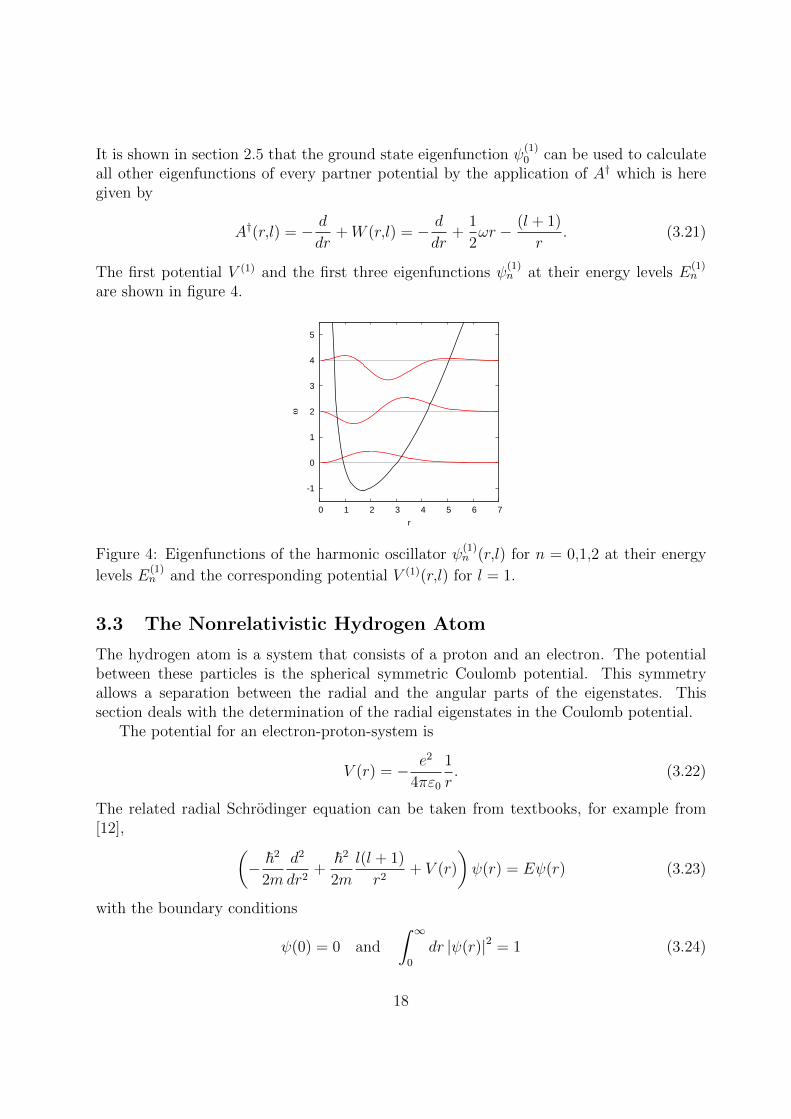
It is shown in section 2.5 that the ground state eigenfunction ψ(1)0 can be used to calculate

all other eigenfunctions of every partner potential by the application of A† which is heregiven by

A†(r,l) = − d

dr+W (r,l) = − d

dr+

1

2ωr − (l + 1)

r. (3.21)

The first potential V (1) and the first three eigenfunctions ψ(1)n at their energy levels E

(1)n

are shown in figure 4.

-1

0

1

2

3

4

5

0 1 2 3 4 5 6 7

ω

r

Figure 4: Eigenfunctions of the harmonic oscillator ψ(1)n (r,l) for n = 0,1,2 at their energy

levels E(1)n and the corresponding potential V (1)(r,l) for l = 1.

3.3 The Nonrelativistic Hydrogen Atom

The hydrogen atom is a system that consists of a proton and an electron. The potentialbetween these particles is the spherical symmetric Coulomb potential. This symmetryallows a separation between the radial and the angular parts of the eigenstates. Thissection deals with the determination of the radial eigenstates in the Coulomb potential.

The potential for an electron-proton-system is

V (r) = − e2

4πε0

1

r. (3.22)

The related radial Schrodinger equation can be taken from textbooks, for example from[12], (

− ~2

2m

d2

dr2+

~2

2m

l(l + 1)

r2+ V (r)

)ψ(r) = Eψ(r) (3.23)

with the boundary conditions

ψ(0) = 0 and

∫ ∞0

dr |ψ(r)|2 = 1 (3.24)

18

for the radial wave function ψ(r). In order to solve the equation the effective potentialV (1)(r) is introduced and the SUSY formalism additionally demands a shift by the groundstate energy E0, so

V (1)(r) = − e2

4πε0

1

r+

~2

2m

l(l + 1)

r2− E0

= W (r)2 − ~√2m

W ′(r). (3.25)

In order to determine the superpotential W (r), an educated guess has to be made. Knowingthe form of the shifted effective potential V (1)(r), this guess is

W (r) = C − D

r. (3.26)

Inserting W (r) in (3.25) yields

V (1) = −2CD

r+

(D − ~√

2m

)D

r2+ C2. (3.27)

The comparison shows that the r-independence can be used to gain the relation

−C2 = E0, (3.28)

furthermore the r-dependent terms yield the equations

e2

4πε0= 2CD and D2 − ~√

2mD =

~2

2ml(l + 1) (3.29)

which can be solved to

C =

√2m

~e2

8πε0(l + 1)and D = − ~√

2ml. (3.30)

This leads directly to the ground state energy E0

E0 = −C2 = − m

2~2

(e4

4πε0(l + 1)

)2

= − ~2

2ma20

1

(l + 1)2(3.31)

with the Bohr radius a0 = 4πε0~2me2

. The determined ground state energy is equal to theliterature values (cf. [12]). Furthermore the now also determined superpotential

W (r) =

√2m

~e2

8πε0(l + 1)− ~√

2m

(l + 1)

r(3.32)

can be used to calculate the partner potential with equation (2.10),

V (2)(r) = − e2

4πε0

1

r+

~2

2m

(l + 1)(l + 2)

r2− E0. (3.33)

19

The potentials are shown in figure 5 for l = 1, they are nonnegative because of the shiftby E0.

0

r

V(1)(r)V(2)(r)

W(r)

Figure 5: The effective radial Coulomb potential V (1)(r), the partner potential V (2)(r) andthe superpotential W (r) for l = 1.

To determine the energy spectrum of the hydrogen atom the SIP formalism is used.Thus the remainder R(l) has to be determined. The SIP condition (2.40) and comparingthe terms that depend on r and l lead to the equation

l2(l2 + 1) = (l1 + 2)(l1 + 1) (3.34)

which is solved by

l2 = f(l1) = l1 + 1. (3.35)

The remainder R(l) is then

R(l) =~2

2ma20

2l + 3

(l + 1)2(l + 2)2. (3.36)

According to the results of section 2.5, the remainder and the relation between two sequentsets of parameters are sufficient to determine all energy values. With l = l1, lk = (l+k−1)and equation (2.45), the energy spectrum of V (1)(r) can be calculated with

E(1)n (l) = E0 +

n∑k=1

R(lk)

=~2

2ma20

(− 1

(l + 1)2+

n∑k=1

2(l + k) + 1

(l + k)2(l + k + 1)2

)(3.37)

20

where the former shift by E0 is reversed in order to get the real spectrum.The formalism for shape invariant potentials allows also to calculate the eigenfunctions

of an electron in the hydrogen atom, which is nontrivial in the textbook examples. Startingwith the formula for the ground state wave function ψ

(1)0 (r) (2.8) and the superpotential

W (r), one gets

ψ(1)0,l (r) = Nrl+1e

− ra0(l+1) (3.38)

with the normalization constant N . The normalization for the only possible value of theangular momentum quantum number, l = 0 yields

ψ(1)0,0(r) = 2a

− 32

0 re− ra0 (3.39)

which is equal to the textbook solution (cf. [12]). Equation (2.50) can be used to determinethe next eigenfunction of H(1)

ψ(1)1,l = N

√a0√

2l + 3

((l + 1)(l + 2)rl+1 − rl+2

a0

)e− r

2a0 (3.40)

and normalizing the function for l = 0 reproduces the textbook equation

ψ(1)1,0(r) = 2(2a0)

− 32

(r − r2

2a0

)e− r

2a0 . (3.41)

The deduced properties can be used to calculated all wave functions of the radial Coulombpotential and the most difficult part of the calculation is the normalization.

3.4 The Dirac Equation

The Dirac equation makes it possible to describe quantum mechanical problems relativisti-cally. In the previous section the exact solution of the nonrelativistic Schrodinger equationfor a Coulomb potential is described. The relativistic Dirac equation of this potential canalso be solved exactly, the solutions for bound states are presented in this section. Startingwith the formulas and notations given in [7] a SUSY quantum mechanical treatment ispossible, this is further described in [3] and [8].

With the parameters

γ =ze2

ch, α1 = m+ E , α2 = m− E (3.42)

the two coupled radial equations (4.13) in [7] which are satisfied by the two-componenteigenfunction (Gk, Fk) can be written as(

dGkdrdFkdr

)+

1

r

(k −γγ −k

)(Gk

Fk

)=

(0 α1

α2 0

)(Gk

Fk

). (3.43)

21

This is the radial eigenfunction after the separation of the angular part of the Dirac equa-tion. The variable k is an eigenvalue of the operator −(σ · L + 1) where L is the angularmomentum operator and can take the values k = ±1,±2,±3,... . k also satisfies |k| = J+ 1

2,

where J is the quantum number for the total spin. In order to solve the coupled equations,the system has to be multiplied with an appropriate matrix D from the left and its inverseD−1 from the right.

D =

(k + s −γ−γ k + s

)with s =

√k2 − γ2 (3.44)

and its inverse

D−1 =1

2s(k + s)

(k + s γγ k + s

)(3.45)

diagonalize

(k −γγ −k

)to

(s 00 −s

)and with the definitions

(GF

)= D

(Gk

Fk

)(3.46)

and ρ = Er the equation (3.43) can be written as

−(m

E+k

s

)F = A†0G(

m

E− k

s

)G = A0F (3.47)

with the operators

A0 =d

dρ− s

ρ+γ

s, A†0 = − d

dρ− s

ρ+γ

s. (3.48)

Like it is done in the previous sections, these adjoint operators can be used to create twosupersymmetric Hamiltonians which can be applied to F and G. Their eigenvalues can bedetermined by using the equations (3.47)

H(1)F = A†0A0F = EF =

(γ2

s2+ 1− m2

E2

)F (3.49)

H(2)G = A0A†0G = EG =

(γ2

s2+ 1− m2

E2

)G (3.50)

with E as new energy eigenvalue for the supersymmetric Hamiltonians. It is used in bothequations which means that every energy eigenvalue of A†0A0 is also an eigenvalue of A0A

†0

22

except for the case A0F = 0. This case can be used to determine the ground state wavefunction to

F0(ρ) = ρse−γρs . (3.51)

The ground state energy eigenvalue E0 is supposed to be zero, which leads to the condition

H(1)F0 = E0F0 =

(γ2

s2+ 1− m2

E20

)F0 = 0

E0 =m√

1 + γ2

s2

. (3.52)

for the energy E0. At this energy the equation (3.50) leads to an unnormalizable eigenstatefor G. To sum up, all eigenstates except for the ground state of F are paired on the sameenergy levels. They are linked with the relations F ∝ A†0G and G ∝ A0F , so the mainrelations of supersymmetric quantum mechanics are obtained.

According to equation (2.4) the superpotential can be gained from the operators A0

and A†0, it is determined to

W (ρ) = −sρ

+γ

s(3.53)

when the substitution x = ~√2mρ is made. This superpotential can be used to calculate the

first two partner potentials

V (1) =s(s− 1)

ρ2+γ2

s2− 2γ

ρ(3.54)

V (2) =(s+ 1)s

ρ2+γ2

s2− 2γ

ρ(3.55)

with the help of (2.6) and (2.10). The ground state wave function F0(ρ) is normalizable,the energy eigenvalue E0 is zero and the comparison between the two potentials shows apossible shape invariance. In order to prove this, the shape invariance condition (2.40) istested

(s1 + 1)s1ρ2

+γ2

s21− 2γ

ρ=s2(s2 − 1)

ρ2+γ2

s22− 2γ

ρ+R(s1). (3.56)

Comparing the ρ−2-dependent terms leads to the conclusion

s2 = s1 + 1⇒ f (n)(s) = s+ n (3.57)

which can be put into (3.56) to determine the ρ-independent remainder to

R(si) =γ2

s2i− γ2

(si + 1)2. (3.58)

23

The energy levels En can now be calculated with (2.45) and the supersymmetric energyeigenvalue En is determined to

En =n∑i=1

(γ2

s2i− γ2

(si + 1)2

)=

n∑i=1

(γ2

(s+ i− 1)2− γ2

(s+ i)2

)=γ2

s2− γ

(s+ n)2(3.49)=

(γ2

s2+ 1− m2

E2n

). (3.59)

Solving (3.59) for the energy levels En gives

En =m√

1 + γ2

(s+n)2

. (3.60)

The shape invariance makes it also possible to determine all eigenfunctions Fn(ρ) by therepeated application of A†n according to (2.49):

Fn(ρ) ∝ (A†0A†1...A

†n−1)ρ

s+ne−γρ

(s+n) (3.61)

with

An =

(d

dρ− s+ n

ρ+

γ

s+ n

); A†n =

(− d

dρ− s+ n

ρ+

γ

s+ n

). (3.62)

Like written above the calculation of Fn determines also Gn according to (3.47). For thecase n = 0, G0 has no normalizable eigenstate at the energy E0. When the two casesof positive and negative values for k are distinguished, inserting in the equations (3.47)shows that normalizable solutions for F0 and G0 can be found for negative values of k withG0 = 0 [3]. This is not possible for positive values of k. The energy (3.60) only dependson k2 and is therefore degenerate, each energy level is a doublet for every level with n > 0.For n = 0 only the negative value of k allows a normalization of F0 and G0, which leadsto a singlet state.

In the calculations above a fixed k is used to determine the fixed parameter s =√k2 − γ2.

In order to determine all energies and eigenfunctions for the values of J = |k| − 12

the re-lation for s can be put into the formulas above. The energy spectrum can then be writtenas

En =m√

1 + γ2

(n+√k2−γ2)2

(3.63)

which is the same result as obtained in textbooks, for example [7] and [12]. The principalquantum number N can be obtained from k and n by N = n+ |k| which leads to

ENJ =m√

1 + γ2

(N−J− 12+√

(J+ 12)2−γ2)2

. (3.64)

24

The energy depends on the principal quantum number N and the total spin J which meansthat the degeneracy of the nonrelativistic calculation is partly removed. (3.64) shows thefine structure in the central Coulomb potential. Together with the doublet structure andthe singlet in the ground state the J dependence creates the eigenvalue spectrum of theDirac equation.

4 Two-Dimensional SUSY QM

The former treatment of supersymmetric quantum mechanics was only done in one dimen-sion. An extension to more space dimensions allows the observation of new phenomena.The description of the formalism is mostly based on [9], [13], [14] and [15].

Before the formalism for a higher dimensional treatment is derived, the main relationsof chapter 2 are presented. From now on for simplicity the factor ~√

2mis set to one. With

the abbreviation ∂ = ddx

the two partner Hamiltonians (2.1) and (2.9) can be written as

H(1) = −∂2 + V (1)(x) = A†A and H(2) = −∂2 + V (2)(x) = AA†. (4.1)

According to (2.16) and (2.17) the wave functions of these Hamiltonians are connected via

ψ(2)n ∝ Aψ

(1)n+1 and ψ

(1)n+1 ∝ A†ψ(2)

n . (4.2)

The reason for this connection is that the Hamiltonians are intertwined. The intertwiningrelations (2.19) play an important role in the description of higher dimensional supersym-metric quantum mechanics.

The described extension to a higher dimensional treatment is mainly based on the useof vector intertwining operators Al(~x); l = 1,2,...,d with

Al(~x) = ∂l + (∂lZ)(~x), A†l (~x) = −∂l + (∂lZ)(~x) (4.3)

with ~x = (x1,x2,...,xd), ∂l =∂

∂xl

where Z(~x) is related to the superpotential by Wl = ∂lZ(~x). The initial Hamiltonian H(1)

can then be quasifactorized in terms of these operators

H(1)(~x) = A†lAl = −∂l∂l + (∂lZ)2(~x)− (∂2l Z)(~x)

= −∂l∂l + V (1)(~x) (4.4)

with the implied sum over all values of l. The first step is the extension to d = 2 dimensionsas simplest case. Similar to the one-dimensional case (2.10), a partner Hamiltonian withanother scalar potential can be constructed

H(3)(~x) = AlA†l = −∂l∂l + (∂lZ)2(~x) + (∂2l Z)(~x)

= −∂l∂l + V (3)(~x). (4.5)

25

In contrast to the one-dimensional case, these two Hamiltonians do not intertwine, butboth of them intertwine with a third Hamiltonian H

(2)ik that depends on a 2 × 2 matrix

potential V(2)ik ;

H(2)ik (~x) = δikH

(1)(~x) + [Ai,A†k]

= −δik∂2l + δik((∂lZ)2(~x)− (∂2l Z)(~x)

)+ 2(∂i∂kZ)(~x)

= −δik∂2l + δikV(1)(~x) + 2(∂i∂kZ)(~x)

= −δik∂2l + V(2)ik (~x) (4.6)

with δik the Kronecker delta. The intertwining operators are mutually orthogonal, theyobey

[A†l ,A†k] = 0 [Al, Ak] = 0 for l 6= k. (4.7)

This orthogonality relation allows to construct the intertwining relations for the threeHamiltonians H(1), H

(2)ik and H(3):

H(1)A†i = A†kH(2)ki ; H

(2)ik Ak = AiH

(1),

H(2)ik εklA

†l = εilA

†lH

(3); εklAlH(2)ki = H(3)εilAl with i,k,l = 1,2 (4.8)

Analogous to the one-dimensional case the intertwining relations determine the similarityof the energy spectra of the participating Hamiltonians. H

(2)ik intertwines with both other

Hamiltonians, while H(1) and H(3) do not intertwine directly. Therefore the two scalarpotentials have the same energy levels as the vector potential up to zero modes of theoperators Al, A

†l . This means that the SUSY formalism allows to reduce a problem related

to a vector potential to the solutions of two scalar potential problems. In contrast to theone-dimensional case the superhamiltonian is not defined as the anticommutator of thesupercharges. This does not influence the connection between the spectra because theintertwining relations still hold. Like in (4.2) the intertwining relations cause a connectionbetween the scalar wave functions of H(1) and H(3) and the vector wave functions of theHamiltonian H

(2)ik .

ψ(2)i (~x) ∝ Aiψ

(1)(~x); ψ(1)(~x) ∝ A†iψ(2)i (~x)

ψ(2)i (~x) ∝ εikA

†kψ

(3)(~x); ψ(3)(~x) ∝ εikAkψ(2)i (~x) with i,k = 1,2 (4.9)

The relations between the Hamiltonians are as in the one-dimensional case based on super-symmetry. So it is again possible to express the Hamiltonians and factorization operatorsvia a superhamiltonian H and supercharges Q,Q†.

H =

H(1) 0 0 0

0 H(2)11 H

(2)12 0

0 H(2)21 H

(2)22 0

0 0 0 H(3)

Q =

0 0 0 0A1 0 0 0A2 0 0 00 A2 −A1 0

=(Q†)†

(4.10)

26

Rearranging the terms can emphasize the similarity to the one-dimensional case and theSUSY algebra (2.21)

H =

(H(1) 0

0 H(2)

); H(1) =

(H(1) 0

0 H(3)

); H(2) =

(H

(2)ik

)(4.11)

Q =

(0 0q 0

)=(Q†)†

; q =

(A1 A†2A2 −A†1

); q† =

(A†1 A†2A2 −A1

)(4.12)

4.1 The Pauli Hamiltonian in Two Dimensions

A nonrelativistic fermion in a given electromagnetic potential is described by the PauliHamiltonian [9], [16], [17]

HP = (i∂i + eAi)2 − µσiBi + U with i = 1,2,3 (4.13)

where e is the charge, µ the magnetic momentum, ~B(~x) = rot ~A(~x) is the magnetic field

which is determined from the vector potential ~A(~x) and U(~x) is the scalar electric potential.σi are the Pauli matrices. HP is a 2 × 2 matrix which acts on a two-component spinorwave function. If the potentials are restricted to potentials that do not depend on one ofthe coordinates (x2 is chosen) and B2 = 0 it can be shown that HP can be identified with

H(2)ik from section 4.

The fermion can move freely in the direction of x2, its wave function can then be written

ψ(~x) = eikx2ψ(x1,x3) (4.14)

and this form can be used to express the Hamiltonian as

HP = −(∂i + eAi)2 + U + (k + eA2)

2 − µσiBi with i = 1,3 (4.15)

The last part of this Hamiltonian in the matrix form is written

−µσiBi = −µ(B3 B1

B1 −B3

)for i = 1,3 (4.16)

and the comparison with H(2)ik in (4.6) shows that the components of the magnetic field

can be identified with

−µB1 = 2(∂1∂3Z)(~x),

−µB3 = (∂21 − ∂23)Z(~x). (4.17)

This allows also the identification of the rest of the Pauli Hamiltonian with a correspondentpart of the supersymmetric partner Hamiltonian

−(∂i + eAi)2 + U + (k + eA2)

2 = −∂2i + (∂iZ)2(~x) with i = 1,3 (4.18)

27

If the field sources are assumed to be absent, the equations

rot ~B = div ~B = 0 (4.19)

lead to the conditions

∂1B1 + ∂3B3 = 0⇔ ∂3(3∂21 − ∂23)Z(~x) = 0,

∂3B1 − ∂1B3 = 0⇔ ∂1(3∂31 − ∂21)Z(~x) = 0. (4.20)

The highest order solution for Z(~x) is according to [17] in fourth order in the variables x1and x3 when the terms with negative power are dropped to get a regular solution withoutpoles,

Z(~x) =1

4a(x21 + x3)

2 + (bx1 + cx3)(x21 + x23) + dx21 + fx23 + 2gx1x3 + hx1 + tx3 (4.21)

depends on eight arbitrary parameters a,b,c,.... The parameter a is restricted to a > 0 ifψ0 = e−Z is a normalizable ground state of H(1). Equations (4.17) can be used to determinethe components B1 and B3 of the magnetic field to

− µB1 = 4(ax1x3 + cx1 + bx3 + g),

− µB3 = 4

(a

2x21 −

a

2x23 + bx1 − cx3 +

d

2− f

2

). (4.22)

The vector potential generates the magnetic field

~B = rot ~A =

∂2A3 − ∂3A2

∂3A1 − ∂1A3

∂1A2 − ∂2A1

. (4.23)

The component B2 is zero, so ∂3A1 = ∂1A3. For the trivial solution A1 = A3 = 0, thecomponent A2 can be calculated straightforwardly from B1 and B3,

A2 =1

2µ

(−1

3ax31 + ax1x

23 − b(x21 − x23) + 2cx1x3 + 2gx3 + (f − d)x1 + γ

). (4.24)

With A1 = A3 = 0, equation (4.18) can be transformed in order to determine the scalarpotential U(~x)

−∂2i + U(~x) + (k + eA2)2 = −∂2i + (∂iZ)2(~x)

→ U(~x) = (∂iZ)2(~x)− (k + eA2)2 = (∂iZ)2(~x)− e2A2

2 (4.25)

with A2 = ke

+ A2. This scalar potential has terms up to sixth order in the coordinates.To sum up for the given constraints it is possible to identify the Pauli Hamiltonian HP

as the Hamiltonian H(2)ik which is part of the superhamiltonian H. Instead of solving an

eigenvalue problem for the 2 × 2 matrix Pauli Hamiltonian it is now possible to use thescalar Hamiltonians H(1) and H(3).

28

4.2 Exact Solution of a Two-Dimensional Model with Real Spec-trum

The two-dimensional treatment of supersymmetric quantum mechanics allows to handledifferent types of problems. A second approach is to deal just with the two scalar Hamil-tonians and to solve a potential which is not amenable to separation of variables via thesolution of a partner potential that is.

4.2.1 The Two-Dimensional Real Singular Morse Potential

The way to keep the focus only on the scalar potentials is to use supercharges of secondorder in derivatives [18]. These supercharges exist in two different variations. In thereducible form they create two partner Hamiltonians that differ only by a constant whichmeans that if one Hamiltonian is amenable to separation of variables, the other one is it,too. In order to create the case described in the introduction of this section, it is necessaryto use irreducible second order components of supercharges. These are written [18],[19]

Q† = gik(~x)∂i∂k + Ci(~x)∂i +B(~x), Q =(Q†)†

(4.26)

while the Hamiltonians

H(i) = −∂l∂l + V (i)(~x); i = 1,2 (4.27)

still satisfy the intertwining relations

H(1)Q† = Q†H(2); QH(1) = H(2)Q. (4.28)

It is important to note that the relation {Q,Q†} = H is now dropped. Nevertheless theHamiltonians and supercharges are chosen in a way that the intertwining relations stillhold. In this particular example the metric gik(~x) is chosen to gik(~x) = diag(1,−1) leadingto the supercharges

Q† =(∂21 − ∂22

)+ Ci∂i +B = 4∂+∂− + C+∂− + C−∂+ +B (4.29)

Q =(∂21 − ∂22

)− Ci∂i +B = 4∂+∂− − C+∂− − C−∂+ +B; i = 1,2 (4.30)

where x± = x1 ± x2, ∂± = ddx±

and C± depend on x±:

C+ = C1 − C2 = C+(x+); C− = C1 + C2 = C−(x−). (4.31)

The potentials and the function B(~x) can be expressed in terms of C± and the functionsF1(2x1), F2(2x2) which satisfy

∂−(C−F ) = −∂+(C+F ). (4.32)

With

F = F1(2x1) + F2(2x2) = F1(x+ + x−) + F2(x+ − x−), (4.33)

29

the general expressions are

B =1

4(C+C− + F1(x+ + x−) + F2(x+ − x−)) ,

V (1) =1

2(C ′+ + C ′−) +

1

8(C2

+ + C2−) +

1

4(F2(x+ − x−)− F1(x+ + x−)) ,

V (2) = −1

2(C ′+ + C ′−) +

1

8(C2

+ + C2−) +

1

4(F2(x+ − x−)− F1(x+ + x−)) . (4.34)

This particular choice of supercharges and potentials satisfies (4.28).As described at the beginning of this section the formalism allows to solve a problem

for one Hamiltonian via finding the solution for the partner Hamiltonian. The case studiedhere is the two-dimensional generalization of the one-dimensional Morse potential. Thedefinitions of C± and F1/2 define the potentials V (1) and V (2):

C+ = 4aα; C− = 4aα · coth(αx−

2

)(4.35)

−VM(x1) =1

4F1(2x1) = −A

(e−2αx1 − 2e−αx1

),

VM(x2) =1

4F2(2x2) = A

(e−2αx2 − 2e−αx2

),

V (1)(~x) = α2a(2a− 1) sinh−2(αx−

2

)+ 4a2α2 + A

(e−2αx1 − 2e−αx1 + e−2αx2 − 2e−αx2

)(4.36)

V (2)(~x) = α2a(2a+ 1) sinh−2(αx−

2

)+ 4a2α2 + A

(e−2αx1 − 2e−αx1 + e−2αx2 − 2e−αx2

)(4.37)

with the real numbers A > 0, α > 0 and a. Both potentials consist of an x-independentterm, two Morse potentials VM(x) = A (e−2αx − 2e−αx) which depend on only one coordi-nate and a sinh−2-term that depends on x− = x1 − x2. The mixing of coordinates in thesinh−2-term is responsible for the fact that the potentials cannot be solved with separationof variables. If the parameters of the model are chosen in a way that separation of variablesis amenable to one of the Hamiltonians belonging to the potentials, the intertwining rela-tions allow it to gain all informations about the other Hamiltonian. The choice of a = −1

2

lets the sinh−2-term in V (2) vanish and makes H(2) amenable to separation of variables,while V (1) still contains a mixing term.

V (1)(~x) = α2(

1 + sinh−2(αx−

2

))+ VM(x1) + VM(x2),

V (2)(~x) = α2 + VM(x1) + VM(x2) (4.38)

Figure 6 shows the one-dimensional Morse potential and the two-dimensional potentialV (1)(~x). The sinh−2-term creates a singularity at x1 = x2 and as it is shown in figure6(a) this singularity deforms the shape of the simple Morse potential. V (2)(~x) on the otherhand is simply the two-dimensional form of VM(x) and matches with V (1)(~x) except for

30

0

x

VM(x)+sinh(αx)-2VM(x)

(a) One-dimensional Morse poten-tial VM (x) and Morse potential withan added sinh−2-term.

-4

-3

-2

-1

x1-4

-3-2

-1x2

(b) Potential V (1)(x1,x2) for a = − 12 and A = α = 1.

Figure 6: One-dimensional Morse potential and the two-dimensional model of a Morsepotential.

the singularity.The Hamiltonian H(2) can be determined to

H(2) = h1(x1) + h2(x2) + α2; hi(xi) = −∂2i + VM(xi); i = 1,2 (4.39)

and it leads to the energy eigenvalues

E(2)m,n = εn + εm + α2 (4.40)

of the symmetric or antisymmetric (for n 6= m) functions

ψ(2),S/An,m = φn(x1)φm(x2)± φm(x1)φn(x2) (4.41)

where εk and φk(x) solve the one-dimensional Morse potential problem [10],[20]:(−∂2 + VM(x)

)φk(x) = εkφk(x); εk = −α2s2k (4.42)

φk = e−ξ2 · ξsk · Φ(−k,2sk + 1; ξ); ξ ≡ 2

√A

αe−αx (4.43)

Φ(a,c;x) = 1 +a

c

x

1!+a(a+ 1)

c(c+ 1)

x2

2!+ ... sk =

√A

α− k − 1

2> 0, k = 0,1,2,... (4.44)

The function Φ(a,c;x) is the confluent hypergeometric function. The equation for theenergy levels of the two-dimensional Hamiltonian H(2) (4.40) acting on the symmetric andantisymmetric wave functions shows that the energy levels are 2-fold degenerate for alllevels with n 6= m.

The intertwining relations can be used to obtain the majority of the levels of H(1), butnot all of them. In general it is possible to think of three different cases which have to beconsidered in order to determine the spectrum and wave functions completely.

31

1. The first attempt to determine the wave functions of H(1) is to use the intertwiningrelations (4.28). The supercharges allow to calculate these wave functions from thewave functions of H(2). The energy levels for the wave functions of H(1) and H(2)

coincide and are given by (4.40).

2. As seen in the one-dimensional case, possible zero modes of Q might occur for H(1).If Q acts on such zero modes no corresponding bound state wave function for H(2)

exist. This means that the intertwining relations cannot be used to obtain the wavefunctions of H(1) from H(2) for this case because no corresponding states in H(2)

exist.

3. If the action of Q on a bound state wave function of H(1) results in a nonnormalizablewave function for H(2) the same problem as in the former case occurs. A state inH(1) without a correspondent state in H(2) cannot be calculated via the intertwiningrelations from the solved system H(2).

In general the intertwining relations (4.28) lead to the connection ψ(1)n,m = Q†ψ

(2)n,m. The

explicit relations can be expanded by using the definition of Q† in (4.29), the explicit formof the wave function (4.43) and the Schrodinger equation (4.42) of the one-dimensionalMorse potential. The derivation is done in appendix A.1 and leads to

ψ(1),Sn,m = Q†ψ(2),A

n,m = (εm − εn)ψ(2),Sn,m +Dψ(2),A

n,m (4.45)

ψ(1),An,m = Q†ψ(2),S

n,m = (εm − εn)ψ(2),An,m +Dψ(2),S

n,m (4.46)

with the operator

D =α2

ξ2 − ξ1[ξ1 + ξ2 + 2ξ1ξ2 (∂ξ1 + ∂ξ2)] (4.47)

for a = −12. The operator Q† is antisymmetric with respect to the exchange of x1 and x2

which explains the calculation of the symmetric functions from the antisymmetric and viceversa. D has a singularity at the line ξ1 = ξ2 or x1 = x2 respectively. The functions ψ

(1),S/An,m

are therefore only normalizable if the functions the operator acts on vanish for ξ1 = ξ2.For this line the symmetrical functions are written

ψ(2),Sn,m (ξ1,ξ2 = ξ1) ∝ φn(ξ1)φm(ξ1)

= e−ξ1ξ2√Aα−1−n−m

1 Φ(−n,2sn + 1; ξ1)Φ(−m,2sn + 1; ξ1). (4.48)

with the definitions of φk and Φ(a,c;x) in (4.43) and (4.44). Φ is just a polynomial and so

ψ(2),Sn,m (ξ1,ξ2 = ξ1) is nonzero for all ξ1 except for ξ1 = 0. Thus the singularity in D can not

be compensated generally and no normalizable antisymmetric functions ψ(1),An,m exist.

32

The existence of symmetric functions depends on the behavior of ψ(2),An,m (ξ1,ξ2 = ξ1).

The functions are written

limξ2→ξ1

ψ(2),An,m (ξ1,ξ2) =

= e−ξ1Φ(−n,2sn + 1; ξ1)Φ(−m,2sm + 1; ξ1) limξ2→ξ1

(ξsn1 ξsm2 − ξsm1 ξsn2 )

= e−ξ1ξ2√Aα−1

1 Φ(−n,2sn + 1; ξ1)Φ(−m,2sm + 1; ξ1) limξ2→ξ1

(ξ−n1 ξ−m2 − ξ−m1 ξ−n2

). (4.49)

The limit of the last factor should be evaluated with the multiplied singularity from theoperator D:

limξ2→ξ1

ξ−n1 ξ−m2 − ξ−m1 ξ−n2

ξ2 − ξ1= ξ−2m1 lim

ξ2→ξ1

ξ−n+m1 − ξ−n+m2

ξ2 − ξ1

= ξ−2m1 limξ2→ξ1

(n−m)ξ−n+m−12

1= (n−m)ξ−n−m+1

1 , (4.50)

where l’Hospital’s rule is used. So the action of D leads to normalizable results for ψ(1),Sn,m .

The behavior of these functions in dependency on m and n can be further investigated.In order to calculate the norm of the wave functions ψ

(1),Sn,m it is helpful to introduce the

operator T = QQ†. It is shown in appendix A.2 that for a = −12

this operator can bewritten as

T = (h1 − h2)2 + 2α2(h1 + h2) + α4, (4.51)

with the definition of hi in (4.39). The action on the antisymmetric functions ψ(2),An,m shows

that they are eigenfunctions of T , the eigenvalues tn,m can be calculated to (cf. A.2)

Tψ(2),An,m = [(εn − εm)2 + 2α2(εn + εm) + α4]ψ(2),A

n,m (4.52)

= α4[(n−m)2 − 1][(sn + sm)2 − 1]ψ(2),An,m ≡ tn,mψ

(2),An,m . (4.53)

Relation (4.53) can be used to determine the norm of the symmetric wave functions

||ψ(1),Sn,m ||2 = 〈ψ(2),A

n,m |QQ†|ψ(2),An,m 〉 = tn,m||ψ(2),A

n,m ||2. (4.54)

Because the antisymmetric function ψ(2),An,m vanishes for m = n, ψ

(1),Sn,m is also zero. The

representation of tn,m in (4.53) shows additionally that tn,n±1 vanishes and with it also

||ψ(1),Sn,n±1||. The norms of ψ

(1),Sn,m with |n−m| > 1 are finite and positive. The values n,m

have an upper limit because of the condition sk > 0 from the solution of the one-dimensionalMorse potential. With the relation (4.44), the range of the parameters is determined to

0 ≤ k < (√Aα− 1

2) with k = n,m.

In addition to these calculations the possible cases for energy levels and wave functionsof H(1) without a normalizable counterpart in the spectrum H(2) have to be examined.

33

The second case of the three cases described above concerns the states of H(1) for whichQψ

(1)n,m = 0. In order to determine these zero modes a property of the system is used. The

comparison of the formulas for Q and Q† shows that generally an exchange a↔ −a leadsto the exchanges Q ↔ Q† and H(1) ↔ H(2). It is shown in [11] that the range for a thatprovides the condition of normalizability of zero modes of Q† and the absence of a fall tothe center is

a ∈(−∞,−1

4− 1

4√

2

). (4.55)

Because of the reflection symmetry of Q and Q†, the condition for normalizable zero modesof Q is a > (1

4+ 1

4√2). Because the value a = −1

2in the investigated model is not in this

range, no normalizable zero modes of Q exist. Additionally the restriction for a destroysthe reflection symmetry because in contrast to Q, Q† has zero modes.

In the last possible case the action of Q on a normalizable eigenfunction of H(1) leadsto a nonnormalizable eigenfunction of H(2). In oder to find out if this case exists, it hasto be examined if Q can affect the normalizability of a state. The Hamiltonian H(1) actsnear x− = 0 effectively as

H(1) ∼ −∂21 − ∂22 + α2 sinh−2(αx−

2

)∼ 1

2(−∂2+ − ∂2−) +

4

x2−. (4.56)

This means that only two different behaviors of the eigenfunctions at the line x− = 0 arepossible,

ψ ∼ x2− or ψ ∼ 1

x−(4.57)

where only the first one is normalizable at x− = 0. The operator Q on the other hand actseffectively as

Q ∼ 4∂+∂− + 2α∂− + 2α2 coth(αx−

2

)+ 2α coth

(αx−2

)∂+

∼ 4∂+∂− + 2α∂− +4α

x−+

4

x−∂+. (4.58)

If the normalizability of a function is unaffected by the action of H(1), it is not transformedto a nonnormalizable function by the action of Q. So this third case does also not lead tonew eigenfunctions of H(1) and all eigenfunctions are determined above.

The energy levels of V (1) are the same as the ones of V (2) except for the zero modes ofQ† calculated above. This can be shown with the intertwining relations

Q†H(2)ψ(2)n,m = E(2)

n,mQ†ψ(2)

n,m = E(2)n,mψ

(1)n,m

= H(1)Q†ψ(2)n,m = H(1)ψ(1)

n,m = E(1)n,mψ

(1)n,m. (4.59)

34

The analysis performed above shows that the antisymmetric wave functions ψ(1),An,m vanish.

Hence the energy levels of H(1) are nondegenerate.To summarize the calculations the wave functions of H(1) are the normalizable sym-

metric wave functions ψ(1),Sn,m = Q†ψ

(2),An,m for |n−m| > 1 and 0 ≤ n,m < (

√Aα− 1

2) at

the nondegenerate energy levels (4.40). The two investigated cases of normalizable wavefunctions of H(1) without a partner in H(2) do not appear, they do not add any levelsto the spectrum. The energy eigenvalues and wave functions of H(1) can be determinedcompletely from the solutions of the problem for V (2) which is amenable for separation ofvariables.

4.2.2 Shape Invariance of the Two-Dimensional Morse Model

The one-dimensional Morse potential belongs to the known shape invariant potentials, itsproperties are listed in Table I of [4]. The SIP-condition (2.40) can also be applied to thetwo-dimensional potentials V (1) and V (2). The parameter for shape invariance is supposedto be a, so it is not set to −1

2anymore, the shape invariance condition reads then

V (1)(~x,ak−1) = V (2)(~x,ak) +R(ak−1). (4.60)

In this section it is shown that this condition can be used to create a chain of two-dimensional potentials with known solutions basing on the former calculations. In orderto simplify the calculations, a shift in the model by 4α2a2 is done. The potentials can thenbe expressed by

V (1)(~x,ak) = α2ak(2ak − 1) sinh−2(αx−

2

)+ VM(x1) + VM(x2),

V (2)(~x,ak) = α2ak(2ak + 1) sinh−2(αx−

2

)+ VM(x1) + VM(x2) (4.61)

and the shift changes physically only the energy of the bound states. The intertwiningrelations and all relations deduced by the supercharges Q and Q† do not change, becausethe supercharges are not changed by the shift and commute with every constant factorin the Hamiltonians. The choice of a as parameter for the shape invariance excludes theoriginal Morse potential parts VM(x1) and VM(x2) from the analysis because they areindependent of a. The ak-dependent part of (4.60) is

α2ak−1(2ak−1 − 1) sinh−2(αx−

2

)= α2ak(2ak + 1) sinh−2

(αx−2

)+R(ak−1). (4.62)

The sinh−2-dependent terms can be compared in order to determine the connection betweenak−1 and ak because R is independent of x1 and x2. Solving this quadratic equation

ak−1(2ak−1 − 1) = ak(2ak + 1) (4.63)

leads to different possible values for ak. The first one is ak = −ak−1 which does not lead toa hierarchy of potentials, this choice would just cause an exchange between the two known

35

potentials. So the choice for the connection of the parameters is the second solution

ak = ak−1 −1

2= a0 −

k

2. (4.64)

The remainder R(ak) as x−-independent term is not needed, it can be set to zero for allak.So the potentials V (1)(~x,ak−1) and V (2)(~x,ak) are shape invariant and at the same time thepotentials with the same parameter ak are supersymmetric partner potentials. This allowsto construct a chain of potentials which are alternately connected via the intertwiningrelations and shape invariance. Using the sign ↔ for a connection via the intertwiningrelations, this chain can be expressed as follows

V (2)(~x,a0)↔ V (1)(~x,a0) = V (2)(~x,a1)↔ V (1)(~x,a1) = V (2)(~x,a2)↔ ...

... = V (2)(~x,ak−1)↔ V (1)(~x,ak−1) = V (2)(~x,ak)↔ V (1)(~x,ak). (4.65)

The model is already examined for the case a = −12

and the condition for a in order toprovide the condition of normalizability of zero modes is a < (−1

4− 1

4√2) according to

(4.55). Increasing k by one leads to a decrease of ak by 12

as it can be seen in equation(4.64); it changes in half-integer steps. It is convenient to set a0 = −1

2, which is the

biggest possible half-integer value, additionally the model with this value for a is alreadycompletely solved.

The wave function of H(2)(~x,a1) can simply be derived from the wave function ofH(1)(~x,a0) by a change of parameters

ψ(2),Sn,m (~x,a1) = ψ(1),S

n,m (~x,a0) = Q†(a0)ψ(2),An,m (~x,a0) (4.66)

for |n−m| > 1. At the same time it is clear that no antisymmetric functions ψ(2),An,m (~x,a1)

exist, because they do not exist for H(1)(a0). The energy levels can be determined withthe formula (4.40) and the SIP-condition (4.60), the shift of the potentials leads to a shiftof α2 compared to the energies determined for a0 in the former section

E(2)(a1)ψ(2),Sn,m (~x,a1) =H(2)(~x,a1)ψ

(2),Sn,m (~x,a1)

=H(1)(~x,a0)−R(a0)ψ(1),Sn,m (~x,a0)

= [εn + εm]ψ(1),Sn,m (~x,a0)

= [εn + εm]ψ(2),Sn,m (~x,a1) (4.67)

with the limitation |n−m| > 1 like above.The intertwining relations allow it to do the next step in order to calculate the wavefunctions of H(1)(~x,a1). In general they can be determined via

ψ(1),An,m (~x,a1) = Q†(a1)ψ

(2),Sn,m ( ~x,a1) = Q†(a1)Q

†(a0)ψ(2),An,m (~x,a0) (4.68)

and no symmetric wave functions exist. Like in the first step the factor Q†(a0)ψ(2),An,m (~x,a0)

could contain zero modes of Q†(a1) leading to vanishing wave functions which would lead

36

to a change of the range for |n−m|. The energy levels of H(1)(~x,a1) are the same as theones determined in (4.67). Instead of calculating the zero modes for this particular Q†(a1),the analysis of these zero modes is performed for the generalized case for all ak.

The steps performed above can be used repeatedly in order to determine the wavefunctions of all members of the chain (4.65). The wave functions

ψ(1)m,n(~x,ak) = Q†(ak)Q

†(ak−1)...Q†(a0)ψ

(2),An,m (~x,a0). (4.69)

change between symmetric and antisymmetric behavior, depending on the number of ac-tions of Q†(a). The energy levels are

E(1)(ak) = E(2)(a0)−k−1∑i=0

R(ai) = E(2)(a0) = εn + εm (4.70)

because R(ak) = 0 and have no degeneracy. The last step to the complete solution forall Hamiltonians H(1)(ak) is the determination of the zero modes of Q†(ak) in order tofind out which levels belong to nonvanishing wave functions. The determination is donein A.3. It requires some algebraic steps and it turns out that the wave functions are onlynonvanishing for |n−m| > (k + 1).As in the analysis for a0 = −1

2the other possibilities for wave functions in the spectrum of

H(1)(~x,ak) that cannot be calculated from the spectrum of H(2)(~x,a0) have to be examined.Zero modes of Q(ak) would again require a positive value of ak, this is not possible dueto the restricted range for a. For the third case the behavior of the Hamiltonian and thesupercharge near the singularity are studied. Near x− = 0, the Hamiltonian acts as

H(1)(ak) ∼1

2(−∂2+ − ∂2−) +

2(k + 1)(k + 2)

x2−(4.71)

and the supercharge as

Q(ak) ∼ 4∂+∂− + 2α∂− +4(k + 1)α

x−+

4(k + 1)2

x−∂+ (4.72)

and again Q(ak) is not able to affect the normalizability of a wave function. Thus theproperty of shape invariance and the intertwining relations can be used not only to deter-mine the wave functions and energy levels of the potential V (2)(~x,a0), which is amenableto separation of variables, but also to solve the problem for a whole chain of potentialsV (1)(~x,ak), V

(2)(~x,ak) via the well-known solution of the one-dimensional Morse potential.It is proven in A.3 by generalizing (4.54) for that the spectra of the related Hamiltoniansare nondegenerate because only symmetric or antisymmetric solutions exist. They can becalculated by equation (4.70) where the indices n,m are restricted by |n−m| > k + 1 and

n,m < (√Aα− 1

2) which means that the number of potentials in the chain with normalizable

wave functions is limited. The wave functions can be determined with the operators Q†(ak)and the original wave functions (4.41) via equation (4.69).

37

5 Conclusions

It is shown in this thesis that the formalism of supersymmetric quantum mechanics hasmultiple uses. The first use is the possibility of solving well-known problems in a newmanner. The factorization method was already used in the early days of quantum me-chanics for the solution of the harmonic oscillator but as shown above it can be used withthe other tools of supersymmetric quantum mechanics to solve the eigenvalue problems ofother potentials. The more important benefit of the method is the possibility to createnew potentials and to determine their eigenvalues and bound state wave functions directlyfrom the original potential. So additionally to the plain solution of fairly easy potentialsthe solution of more complex potentials can be obtained. This can also be seen in thefirst example of the two-dimensional treatment. The introduced formalism can be usedto solve the sketched two-dimensional eigenvalue problem for the Pauli Hamiltonian viascalar Hamiltonians. Of course a two-dimensional treatment is not sufficient for the so-lution of complicated three-dimensional problems but the example gives an insight in theusefulness of higher-dimensional supersymmetric quantum mechanics. The last exampleis the most complicated one in this thesis. It is only one example for the solution of atwo-dimensional potential that is not amenable to separation of variables, [9] names alsogeneralized Poschl-Teller and Scarf II potentials as problems that can be solved with thesame treatment. This example of the two-dimensional Morse potential shows even morethan the others that supersymmetric quantum mechanics can be the key to the solutionof complicated potentials. Furthermore the well-known solutions of the one-dimensionalproblem can be used to determine the bound state wave functions and energy levels of awhole class of two-dimensional Morse potentials with the concept of shape invariance.

The main goals of the thesis were on the one hand to present the basic formalismof supersymmetric quantum mechanics and its application to basic examples and on theother hand to show a more complicated extension of the formalism. The presentation ofthe content in section 2 on an undergraduate level can already be found in several papers,theses and occasional in quantum mechanics books. The derivation of the formalism isstraightforward and does not cause major problems for a student who finished a quantummechanics course. However the research in the field of supersymmetric quantum mechanicsoffers many different approaches for the use and the extension of this formalism. Most ofthese fields of application are presented on a high level and require a lot of effort to reachan understanding for an undergraduate student. So another goal of the second part of thisthesis is to explain at least a small part of higher-dimensional supersymmetric quantummechanics on an educational level. The two presented examples cover only a part of thehigher-dimensional treatment and already this topic offers many more examples for the useof supersymmetric quantum mechanics. The summary on an undergraduate level could bedone for a wide range of already examined applications. So additionally to the examinationof different applications of the formalism, the presentation of already known results givesa perspective for future works and theses on this topic.

38

A Derivations

A.1 Connection between the Wave Functions in the Two-DimensionalMorse Potential

The definition of C+ and C− in (4.35) allows to calculate C1 and C2 to

C1 =1

2(C− + C+) = 2aα

[coth

(αx−2

)+ 1],

C2 =1

2(C− − C+) = 2aα

[coth

(αx−2

)− 1]

(A.1)

and to insert these expressions in the explicit form of Q† in (4.29):

Q†ψ(2),An,m

=

{(∂21 − ∂22

)− Ci∂i +

1

4(C+C− + F1(x+ + x−) + F2(x+ − x−))

}ψ(2),An,m

={

(∂21 − ∂22) + 2aα[(

coth(αx−

2

)+ 1)∂1 +

(coth

(αx−2

)− 1)∂2

]+B

}ψ(2),An,m (A.2)

with B = 4a2α2 coth(αx−

2

)− VM(x1) + VM(x2).

The action of the single summands on the wave functions can be examined individually.The action of the second derivatives and the one-dimensional Morse potentials can bedetermined by the Schrodinger equation (4.42)[

∂21 − ∂22 − VM(x1) + VM(x2)]ψ(2),An,m

(4.39)= [−h1 + h2] [φn(x1)φm(x2)− φm(x1)φn(x2)]

(4.42)= −εnφn(x1)φm(x2) + εmφm(x1)φn(x2) + εmφn(x1)φm(x2)− εnφm(x1)φn(x2)

= (εm − εn)[φn(x1)φm(x2) + φm(x1)φn(x2)]

= (εm − εn)ψ(2),Sn,m . (A.3)

The second part of (A.2) is

2aα[(

coth(αx−

2

)+ 1)∂1 +

(coth

(αx−2

)− 1)∂2 + 2aα coth

(αx−2

)]ψ(2),An,m

= 2aα

[2eαx−

eαx− − 1∂1 +

2

eαx− − 1∂2 + 2aα

eαx− + 1

eαx− − 1

]ψ(2),An,m . (A.4)

39

The relation ξ = 2√Aαe−αx given in (4.43) can be used to deduce some helpful equations:

ξi =2√A

αe−αxi ⇔ xi = − 1

αln

(αξi

2√A

),

∂ξi =∂

∂ξi=

∂

∂xi

∂xi∂ξi

= − 1

αξi∂i ⇔ ∂i = −αξi∂ξi ,

eαx− = eα(x1−x2) = eαx1e−αx2 =ξ2ξ1,

eαx− − 1 =ξ2ξ1− 1 =

ξ2 − ξ1ξ1

,

2e(αx−)

eαx− − 1= 2

ξ2ξ2 − ξ1

;2

eαx− − 1= 2

ξ1ξ2 − ξ1

;e(αx−) + 1

e(αx−) − 1=ξ2 + ξ1ξ2 − ξ1

. (A.5)

With these equations (A.4) can be rewritten to

2aα

[2

ξ2ξ2 − ξ1

(−αξ1∂ξ1) + 2ξ1

ξ2 − ξ1(−αξ2∂ξ2) + 2aα

ξ2 + ξ1ξ2 − ξ1

]ψ(2),An,m

=4a2α2

ξ2 − ξ1

[ξ1 + ξ2 −

ξ1ξ2a

(∂ξ1 + ∂ξ2)

]ψ(2),An,m

≡ Dψ(2),An,m (A.6)

which together with the first part leads directly to the given equations.

A.2 The Operator T

The determination of T requires the multiplication of the two operators Q (4.30) and Q†

(4.29), for the examined model they are written

Q = −h1 + h2 + 4a2α2 coth(αx2

2

)− 4aα∂− − 4aα coth

(αx22

)∂+,

Q† = −h1 + h2 + 4a2α2 coth(αx2

2

)+ 4aα∂− + 4aα coth

(αx22

)∂+ (A.7)

with the introduced hi = −∂i + VM(xi). The calculation of QQ† contains the applicationof the chain rule for the partial derivative ∂−. The derivation of the Morse potentials∂±(−VM(x1)+VM(x2)) is done with the representation ∂± = 1

2(∂1±∂2) and to simplify the

calculation the summands containing a Morse potential can be rearranged separately. Therest of the calculation is done straightforwardly, the factor a is set to −1

2and the result is

T = (h1 − h2)2 + 2α2(h1 + h2) + α4 (A.8)

The calculations of the eigenvalues tn,m can be done straightforwardly with the defi-nitions of the wave functions (4.41) and the Schrodinger equation of the one-dimensional

40

Morse potential (4.42). For clarity the abbreviations ηa = φn(x1)φm(x2) and ηb = φm(x1)φn(x2)are used.

Tψ(2),An,m =[h21 − 2h1h2 +2

2 +2α2(h1 + h2) + α4][ηa − ηb]=ε2nηa − ε2mηb − 2εnεmηa + 2εnεmηb + ε2mηa − ε2nηb+

+ 2α2(εnηa − εmηb + εmηa − εnηb) + α4(ηa − ηb)=(ε2n − 2εnεm + ε2m)(ηa − ηb) + 2α2(εn + εm)(ηa − ηb) + α4(ηa − ηb)=[(εn − εm)2 + 2α(εn + εm) + α4]ψ(2),A

n,m . (A.9)

The equivalence of (4.52) and (4.53) can be shown with the definition of sk in (4.44) whichleads to the relation n−m = sm − sn and the definition of εk in (4.42).

α4[(n−m)2 − 1][(sn + sm)2 − 1]

= α4[(sn − sm)2 − 1][(sn + sm)2 − 1]

= α4[(s2n − s2m)2 − (sn − sm)2 − (sm + sn)2 + 1]

= α4[(s2n − s2m)2 − 2(s2n + s2m) + 1]

= (εn − εm)2 + 2α2(εn + εm) + α4. (A.10)

A.3 Zero Modes of Q†(ak)

Reference [11] offers a starting point to deduce the zero modes of Q†(ak) by beginning withthe calculation of the relation between the operators T (ak) and T (ak−1) with T (ak) = Q(ak)Q

†(ak),as above. The calculation is similar to the one done in A.2, it additionally requires the useof ak = −k+1

2which was determined in (4.64) and leads to the relation

Q(ak)Q†(ak) = Q†(ak−1)Q(ak−1) + α2(2k + 1)[2H(1)(~x,ak−1) + α2(2k2 + 2k + 1)]. (A.11)

The operators T (ak) can again be used to determine the norm of a wave function ψ(1)m,n(~x,ak)

and the form of equation (A.11) can be used to determine a general formula. The norm fork = 0 was computed in (4.54) and contains the factor tn,m. The norm for k = 1 accordingto equation (4.69) is

||ψ(1)n,m(~x,a1)||2 = 〈ψ(2,A)

n,m (~x,a0)|Q(a0)Q(a1)Q†(a1)Q

†(a0)|ψ(2,A)n,m (~x,a0)〉

= 〈ψ(2,A)n,m (~x,a0)|Q(a0)

[Q†(a0)Q(a0) + 3α2[2H(1)(~x,a0) + 5α2]

]Q†(a0)|ψ(2,A)

n,m (~x,a0)〉=(t2n,m + tn,m · 3α2[2(εn + εm) + 5α2]

)||ψ(2,A)

n,m (~x,a0)||2

= tn,m(tn,m + 3α2[2(εn + εm) + 5α2]

)||ψ(2,A)

n,m (~x,a0)||2, (A.12)

where the intertwining relations are used to determine

H(1)(~x,a0)Q†(a0)|ψ(2,A)

n,m (~x,a0)〉 = Q†(a0)H(2)(~x,a0)|ψ(2,A)

n,m (~x,a0)〉= (εn + εm)Q†(a0)|ψ(2,A)

n,m (~x,a0)〉 (A.13)

41

This simplest case already shows that a recursion occurs. Carrying out the next steps andusing the intertwining relations, the SIP-condition and (A.11) lead to the general result

||ψ(1)n,m(~x,ak)||2 = 〈ψ(2,A)

n,m (~x,a0)|Q(a0)...Q(ak)Q†(ak)...Q

†(a0)|ψ(2,A)n,m (~x,a0)〉

= 〈ψ(2,A)n,m (~x,a0)|T (a0) · (T (a0) + Γ1) · ... · (T (a0) + Γ1 + ...+ Γk) |ψ(2,A)

n,m (~x,a0)〉 (A.14)

with Γk = α2(2k + 1)[2H(1)(~x,ak−1) + α2(2k2 + 2k + 1)]. (A.15)

The goal of the following steps is the factorization of the prefactors in (A.14) in termsof (n−m). The sums of the Γk terms in the norm can with (A.15) be written as

k∑j=1

γj =k∑j=1

[2α2(2j + 1)(εn + εm) + α4(2j + 1)(2j2 + 2j + 1)

]=

k∑j=1

[2α2(2j + 1)(εn + εm) + α4[(j + 1)4 − j4]

]= 2α2k(k + 2)(εn + εm) + α4[(k + 1)4 − 1]

= α4[−2(s2n + s2m)k(k + 2) + (k + 1)4 − 1] (A.16)

where γk denote the eigenvalues of Γk. The norm contains the product over the sums plusthe eigenvalues tn,m

k∏j=1

(tn,m +

j∑i=1

γi

)

= α4k

k∏j=1

{[(n−m)2 − 1][(sn + sm)2 − 1]− 2(s2n + s2m)j(j + 2) + (j + 1)4 − 1

}(A.17)

which can be factorized with some algebra. The norm can then be determined to

||ψ(1)n,m(~x,ak)||2 = α4k||ψ(2)

n,m(~x,a0)||2 tn,mk∏j=1

[(n−m)2 − (j + 1)2][(sn + sm)2 − (j + 1)2].

(A.18)

It was already shown that the norm of the wave functions ψ(1)n,m(~x,ak) vanishes for |n−m| ≤ 1.

The difference in the factor containing (n − m) in equation(A.18) shows that the lowerboundary for nonvanishing wave functions depends on k. Bound state wave functions onlyexist for |n−m| > (k + 1).

42

References

[1] E. Witten, Nuclear Physics B 188, 513 (1981).

[2] F. Cooper, A. Khare, and U. Sukhatme, Physics Reports 251, 267 (1995).

[3] C. V. Sukumar, AIP Conference Proceedings 744, 166 (2004).

[4] R. Dutt, A. Khare, and U. P. Sukhatme, Am. J. Phys 56, 163 (1988).

[5] E. Nygren, Supersymmetric quantum mechanics, Bachelor’s thesis, University ofBern, 2010.

[6] A. Oeftiger, Supersymmetric quantum mechanics, Bachelor’s thesis, University ofBern, 2010.

[7] J. D. Bjorken and S. D. Drell, Relativistic quantum mechanics, McGraw-Hill, NewYork, 2 edition, 1964.

[8] M. Broekroelofs, Supersymmetry in quantum mechanics, Bachelor’s thesis, Rijksuni-versiteit Groningen, Groningen, 2007.

[9] A. Andrianov and M. Ioffe, J.Phys. A45, 503001 (2012).

[10] M. V. Ioffe, F. Cannata, and D. N. Nishnianidze, Theoretical and MathematicalPhysics 148, 960 (2006).

[11] M. Ioffe and D. Nishnianidze, Phys.Rev. A76, 052114 (2007).

[12] G. Munster, Quantentheorie, Walter de Gruyter, 2010.

[13] A. A. Andrianov, N. V. Borisov, and M. V. Ioffe, Physics Letters A 105, 19 (1984).

[14] A. A. Andrianov, N. V. Borisov, M. V. Ioffe, and M. I. Eides, Theoretical and Math-ematical Physics 61, 965 (1984).

[15] A. A. Andrianov, N. Borisov, and M. V. Ioffe, JETP Lett. 39, 93 (1984).

[16] F. Schwabl, Quantenmechanik (QM I), Springer-Verlag, Berlin Heidelberg New York,7. aufl. edition, 2007.

[17] A. A. Andrianov and M. V. Ioffe, Physics Letters B 205, 507 (1988).

[18] M. V. Ioffe, J.Phys. A37, 10363 (2004).

[19] A. A. Andrianov, M. V. Ioffe, and D. Nishnianidze, (1996).

[20] H. Bateman, A. Erdelyi, W. Magnus, F. Oberhettinger, and F. G. Tricomi, Highertranscendental functions, volume 1, McGraw-Hill New York, 1955.

43