supernova rates, rise-times, and their relations to ... · 4.9 fom for different fit conditions...
TRANSCRIPT
SUPERNOVA RATES, RISE-TIMES, AND THEIR RELATIONS TO PROGENITORS
by
Santiago Gonzalez Gaitan
A thesis submitted in conformity with the requirementsfor the degree of Doctor of Philosophy
Graduate Department of Astronomy and AstrophysicsUniversity of Toronto
c© Copyright by Santiago Gonzalez Gaitan 2011

Abstract
Supernova Rates, Rise-Times, and their Relations to Progenitors
Santiago Gonzalez Gaitan
Doctor of Philosophy
Graduate Department of Astronomy and Astrophysics
University of Toronto
2011
Supernovae are fundamental in astronomy: they inject high mass elements into the interstel-
lar medium enriching the chemistry of galaxies, they feed processes of star formation and
active galactic nuclei, and they have been a key for the developments in cosmology of the past
decades.
This dissertation presents a set of subluminous type Ia supernovae (SNe Ia) at z > 0.1
from the Supernova Legacy Survey (SNLS). These faint and short-lived transients are found in
massive and passive host galaxies. We measure a volumetric rate as a function of redshift that
is different from the normal SN Ia population. The observations point towards a long delay
time since the birth of the progenitors systems and argue for progenitor stars of initial low
mass.
We calculate a stretch-corrected rise-time since explosion to maximum brightness for dif-
ferent sets of SNe Ia. We find that a fiducial 17 day quadratic rise is sufficient to explain all
SNe Ia, including subluminous ones, arguing for their homogeneity throughout the entire
light-curve. Subluminous SNe Ia are powered by as little as 0.05 M⊙of56Ni synthesized in the
explosion. Theoretical models need to explain these challenging weak explosions within the
framework of SNe Ia.
Finally, we develop one of the first robust automated techniques to identify plateau super-
novae (SNe IIP) in large photometric transient surveys. This simple method was tested with a
variety of real and simulated SN samples and proved to be effective across different redshifts.
Such a photometric typingwill be of great power for coming surveys and will allow numerous
scientific studies of SNe IIP.
ii

Acknowledgements
I am very thankful to my supervisor, Ray Carlberg, for a healthy work balance, providing
support when needed but also trust and freedom to advance as a scientist and allowing me
to keep priorities in place. To the Toronto-based SNLS collaboration, Alex, Mark, Kathy and
Andy, I am extremely grateful for your incredible help, patience and advice, but especially
for your coolness. I thank the whole SNLS team for making this survey a success and this
thesis possible. To Dae-Sik Moon, Marten van Kerkwijk and Bob Abraham for very helpful
discussions and tips, and to Brian Schmidt for insightful comments that improved this thesis.
I thank Andrea Pastorello for the use of unpublishded supernova data.
I would like to thank the constant support of my family, particularly my mother, and of the
Toronto family, i. e. all my friends: you are the ones that make life a happy adventure! Almost
no et al.’s here: Dani, Erinilla, Pollote, Nixon, Sherrylein, Zaki, Marcono, Pookie, Vietta, Mar-
ija, Preethi, Nandao, Bananne, Majid, Azin, Harui, Laura, Ricardinho and Yu-Min, Justin and
Johanna, Fedex, Cata y Caja, Kai, Lauretta, Benkelein, Patrick, Kev, Ivana, Sasa, Kora, Mari-
angela, Fer (special thanks for super useful discussions!), Moni y Sebas, Fermın y Ana, Inigo,
Alexis, Aleks, Pooh, Benito y Caterina, Tomek, Oliver C., Jeanine, Tony, Lucie et Mika, Renbin,
Summer and Willy, Mikhael and Tracey, Bindo, Alex, Darrell, Mimi, and many more... (et. al.,
after all).
At last, I thank all the great beings working for a better tomorrow. They remindme of what
is important and all that remains to be done. To God.
iii
Contents
1 Introduction 1
1.1 SN classification . . . . . . . . . . . . . . . . . . . . . . . . . . . . . . . . . . . . . 1
1.2 Supernovae Type Ia . . . . . . . . . . . . . . . . . . . . . . . . . . . . . . . . . . . 3
1.2.1 Observational characteristics . . . . . . . . . . . . . . . . . . . . . . . . . 3
1.2.2 Explosion and Progenitor scenarios . . . . . . . . . . . . . . . . . . . . . 4
1.2.3 SNe Ia as distance indicators . . . . . . . . . . . . . . . . . . . . . . . . . 8
1.3 Core-collapse supernovae . . . . . . . . . . . . . . . . . . . . . . . . . . . . . . . 12
1.3.1 Observational characteristics . . . . . . . . . . . . . . . . . . . . . . . . . 12
1.3.2 Theory of explosion . . . . . . . . . . . . . . . . . . . . . . . . . . . . . . 13
1.3.3 Progenitor scenarios . . . . . . . . . . . . . . . . . . . . . . . . . . . . . . 15
1.3.4 SNe IIP as distance indicators . . . . . . . . . . . . . . . . . . . . . . . . . 17
1.4 Motivation for this dissertation . . . . . . . . . . . . . . . . . . . . . . . . . . . . 18
2 Subluminous SNe Ia at High-z from the SNLS 20
2.1 Introduction . . . . . . . . . . . . . . . . . . . . . . . . . . . . . . . . . . . . . . . 20
2.2 Local relations for low-stretch SNe Ia . . . . . . . . . . . . . . . . . . . . . . . . . 23
2.2.1 Color-stretch relations . . . . . . . . . . . . . . . . . . . . . . . . . . . . . 24
2.2.2 Luminosity-color-stretch . . . . . . . . . . . . . . . . . . . . . . . . . . . . 27
2.3 High-z low-stretch candidate selection . . . . . . . . . . . . . . . . . . . . . . . . 30
2.3.1 Redshift estimation and LC fit . . . . . . . . . . . . . . . . . . . . . . . . 30
2.3.2 Final candidates . . . . . . . . . . . . . . . . . . . . . . . . . . . . . . . . . 33
At z ≤ 0.6 . . . . . . . . . . . . . . . . . . . . . . . . . . . . . . . . . . . . 35
At z > 0.6 . . . . . . . . . . . . . . . . . . . . . . . . . . . . . . . . . . . . 35
2.4 Low-stretch SN Ia rate evolution . . . . . . . . . . . . . . . . . . . . . . . . . . . 39
2.4.1 Detection efficiencies . . . . . . . . . . . . . . . . . . . . . . . . . . . . . . 40
2.4.2 SN Ia Rates and Monte-Carlo simulations . . . . . . . . . . . . . . . . . . 41
2.4.3 Contamination uncertainties . . . . . . . . . . . . . . . . . . . . . . . . . 50
iv

2.5 Discussion . . . . . . . . . . . . . . . . . . . . . . . . . . . . . . . . . . . . . . . . 52
2.5.1 Low-z subluminous rate . . . . . . . . . . . . . . . . . . . . . . . . . . . . 52
2.5.2 Power-law evolution . . . . . . . . . . . . . . . . . . . . . . . . . . . . . . 52
2.5.3 Delayed component model . . . . . . . . . . . . . . . . . . . . . . . . . . 53
2.5.4 Delay-time distributions . . . . . . . . . . . . . . . . . . . . . . . . . . . . 55
2.5.5 Extremely low-s SNe Ia . . . . . . . . . . . . . . . . . . . . . . . . . . . . 57
2.6 Summary . . . . . . . . . . . . . . . . . . . . . . . . . . . . . . . . . . . . . . . . . 58
3 The Rise-Time of Normal and Subluminous Type Ia Supernovae 62
3.1 Introduction . . . . . . . . . . . . . . . . . . . . . . . . . . . . . . . . . . . . . . . 62
3.2 Rise-time fit . . . . . . . . . . . . . . . . . . . . . . . . . . . . . . . . . . . . . . . 65
3.2.1 Lightcurve parameterization . . . . . . . . . . . . . . . . . . . . . . . . . 65
3.2.2 Rise-time parameterization . . . . . . . . . . . . . . . . . . . . . . . . . . 66
3.2.3 56Ni radioactive decay . . . . . . . . . . . . . . . . . . . . . . . . . . . . . 66
3.3 Data . . . . . . . . . . . . . . . . . . . . . . . . . . . . . . . . . . . . . . . . . . . . 67
3.3.1 SNLS . . . . . . . . . . . . . . . . . . . . . . . . . . . . . . . . . . . . . . . 67
3.3.2 Low-z and SDSS . . . . . . . . . . . . . . . . . . . . . . . . . . . . . . . . 68
3.4 Analysis . . . . . . . . . . . . . . . . . . . . . . . . . . . . . . . . . . . . . . . . . 69
3.4.1 Rise-time calculation . . . . . . . . . . . . . . . . . . . . . . . . . . . . . . 69
3.4.2 Comparison of single- and two-stretch fits . . . . . . . . . . . . . . . . . 72
3.4.3 Comparison of different templates . . . . . . . . . . . . . . . . . . . . . . 75
3.4.4 Comparison with SALT2 . . . . . . . . . . . . . . . . . . . . . . . . . . . . 78
3.4.5 Transition Epoch . . . . . . . . . . . . . . . . . . . . . . . . . . . . . . . . 79
3.4.6 Zero scale b . . . . . . . . . . . . . . . . . . . . . . . . . . . . . . . . . . . 80
3.4.7 Different rise power laws . . . . . . . . . . . . . . . . . . . . . . . . . . . 81
3.5 Results and Discussion . . . . . . . . . . . . . . . . . . . . . . . . . . . . . . . . . 83
3.5.1 Comparison to previous studies . . . . . . . . . . . . . . . . . . . . . . . 83
3.5.2 56Ni masses . . . . . . . . . . . . . . . . . . . . . . . . . . . . . . . . . . . 85
3.5.3 Secondary lightcurve parameters . . . . . . . . . . . . . . . . . . . . . . . 86
3.6 Conclusions . . . . . . . . . . . . . . . . . . . . . . . . . . . . . . . . . . . . . . . 89
4 A Simple Photometric Typing Technique for Plateau Supernovae 91
4.1 Introduction . . . . . . . . . . . . . . . . . . . . . . . . . . . . . . . . . . . . . . . 91
4.2 Typing evaluation . . . . . . . . . . . . . . . . . . . . . . . . . . . . . . . . . . . . 93
4.3 Samples . . . . . . . . . . . . . . . . . . . . . . . . . . . . . . . . . . . . . . . . . 94
4.4 Method . . . . . . . . . . . . . . . . . . . . . . . . . . . . . . . . . . . . . . . . . . 98
4.4.1 Maximum epoch . . . . . . . . . . . . . . . . . . . . . . . . . . . . . . . . 98
v
4.4.2 Simple linear post-maximum fit . . . . . . . . . . . . . . . . . . . . . . . 99
4.4.3 Multi-band fit parameters and probability distributions . . . . . . . . . . 99
4.4.4 Variation of fitting conditions . . . . . . . . . . . . . . . . . . . . . . . . . 107
Fit duration . . . . . . . . . . . . . . . . . . . . . . . . . . . . . . . . . . . 108
Data requirements . . . . . . . . . . . . . . . . . . . . . . . . . . . . . . . 108
4.4.5 Redshift information . . . . . . . . . . . . . . . . . . . . . . . . . . . . . . 111
4.4.6 Training set . . . . . . . . . . . . . . . . . . . . . . . . . . . . . . . . . . . 112
4.5 Results . . . . . . . . . . . . . . . . . . . . . . . . . . . . . . . . . . . . . . . . . . 114
4.6 Conclusions . . . . . . . . . . . . . . . . . . . . . . . . . . . . . . . . . . . . . . . 117
5 Summary and Outlook 119
5.1 Type Ia supernovae . . . . . . . . . . . . . . . . . . . . . . . . . . . . . . . . . . . 119
5.2 Plateau supernovae . . . . . . . . . . . . . . . . . . . . . . . . . . . . . . . . . . . 122
Bibliography 125
vi

List of Tables
1.1 Supernova classification . . . . . . . . . . . . . . . . . . . . . . . . . . . . . . . . 2
2.1 Nearby low-s objects that passed the observation and fit culls . . . . . . . . . . 46
2.2 Nearby non-Ia SNe with acceptable SN Ia SiFTO fits, enough data coverage and
fitted s ≤ 0.8. . . . . . . . . . . . . . . . . . . . . . . . . . . . . . . . . . . . . . . . 47
2.3 Culls applied to the training sample . . . . . . . . . . . . . . . . . . . . . . . . . 47
2.4 Culls applied to the SNLS sample . . . . . . . . . . . . . . . . . . . . . . . . . . . 47
2.5 SNLS low-s candidates at z ≤ 0.6 . . . . . . . . . . . . . . . . . . . . . . . . . . . 48
2.6 Volumetric rates for the subluminous SNe Ia in the SNLS . . . . . . . . . . . . . 49
2.7 Estimated contamination percentages . . . . . . . . . . . . . . . . . . . . . . . . 51
3.1 Nearby objects used in the rise-time calculation . . . . . . . . . . . . . . . . . . . 68
3.2 Stretch-corrected rise-time fit results for the single- and two-stretch techniques 73
3.3 Stretch-corrected rise-time systematic uncertainties . . . . . . . . . . . . . . . . 77
3.4 Stretch-corrected rise-time and power-exponents fit results for the different stretch
samples in the SNLS . . . . . . . . . . . . . . . . . . . . . . . . . . . . . . . . . . 81
4.1 SN samples used to investigate the simple SN IIP typing technique . . . . . . . 94
4.2 Nearby supernovae used in the SN IIP typing . . . . . . . . . . . . . . . . . . . . 95
4.3 Duration and data requirement of fitted region for each SN sample . . . . . . . 110
4.4 Efficiencies, purities and FoMs for each SN sample . . . . . . . . . . . . . . . . . 118
vii

List of Figures
1.1 SN Ia lightcurves . . . . . . . . . . . . . . . . . . . . . . . . . . . . . . . . . . . . 3
1.2 SN Ia Hubble Diagram . . . . . . . . . . . . . . . . . . . . . . . . . . . . . . . . . 9
1.3 CC SNe lightcurves . . . . . . . . . . . . . . . . . . . . . . . . . . . . . . . . . . . 13
2.1 Example SiFTO LC fits for low-s SNe Ia . . . . . . . . . . . . . . . . . . . . . . . 25
2.2 Color as a function of stretch for the training sample . . . . . . . . . . . . . . . . 27
2.3 Absolute magnitude vs color and stretch for the training sample . . . . . . . . . 29
2.4 Change in stretch due to redshift variation . . . . . . . . . . . . . . . . . . . . . 32
2.5 Flow diagram of SN Ia candidate selection and photometric redshift measurement 33
2.6 Photometric redshifts vs spectroscopic redshifts for the SN Ia candidates . . . . 34
2.7 Color-stretch, magnitude-color and magnitude-stretch for the SN Ia candidates 36
2.8 Final distributions in redshift, stretch and color of the z < 0.6 SN Ia photometric
sample . . . . . . . . . . . . . . . . . . . . . . . . . . . . . . . . . . . . . . . . . . 37
2.9 Distribution in ∆mag of the final low-s candidate sample . . . . . . . . . . . . . 38
2.10 Color as a function of redshift for the final photometric SN Ia sample . . . . . . 38
2.11 Absolute magnitude vs color for the low-s SN Ia sample . . . . . . . . . . . . . 40
2.12 Efficiencies for the SN Ia photometric sample . . . . . . . . . . . . . . . . . . . . 42
2.13 Volumetric rate of low-s SNe Ia as a function of redshift . . . . . . . . . . . . . . 43
2.14 Example of observed and corrected color distribution for low-s at 0.7 < z < 0.9 44
2.15 Host properties for SN Ia candidates . . . . . . . . . . . . . . . . . . . . . . . . . 53
2.16 Best fit DTDs to the low-s SN Ia rate . . . . . . . . . . . . . . . . . . . . . . . . . 57
2.17 Extremely low-s candidate . . . . . . . . . . . . . . . . . . . . . . . . . . . . . . . 58
2.18 Rate evolution for low-s candidates (s ≤ 0.8) and extremely low-s candidates
with s ≤ 0.65 from the SNLS . . . . . . . . . . . . . . . . . . . . . . . . . . . . . . 59
3.1 Overlaid B-band restframe lightcurves of low- and normal-stretch SNe Ia from
the SNLS . . . . . . . . . . . . . . . . . . . . . . . . . . . . . . . . . . . . . . . . . 70
3.2 Overlaid B-band restframe lightcurves of low- and normal-stretch SNe Ia from
the SNLS in the early rise . . . . . . . . . . . . . . . . . . . . . . . . . . . . . . . . 71
viii

3.3 Distribution of 100MC stretch-corrected rise-time fits to low- and normal-stretch
SNe Ia. . . . . . . . . . . . . . . . . . . . . . . . . . . . . . . . . . . . . . . . . . . 72
3.4 Comparison of rise- and fall-stretch for SNLS SNe Ia calculated with the 2-s vs
1-s technique . . . . . . . . . . . . . . . . . . . . . . . . . . . . . . . . . . . . . . . 75
3.5 Difference of peak date and peak date error calculated with the 1-s and the 2-s
techniques for the SNLS . . . . . . . . . . . . . . . . . . . . . . . . . . . . . . . . 76
3.6 Different SN Ia light-curve templates . . . . . . . . . . . . . . . . . . . . . . . . . 77
3.7 Stretch comparison between lightcurve fits of different templates . . . . . . . . 78
3.8 Comparison of SiFTO stretch and SALT2 X1 . . . . . . . . . . . . . . . . . . . . 79
3.9 Stretch-corrected rise-time as a function of the transition epoch . . . . . . . . . 80
3.10 Rise-time as a function of zero scale and power exponent . . . . . . . . . . . . . 82
3.11 Individual rise-times as a function of B-band magnitude at maximum and X1 . 84
3.12 Distribution 56Ni masses for the normal- and low-s SN Ia SNLS samples based
on 1-s and 2-s fits . . . . . . . . . . . . . . . . . . . . . . . . . . . . . . . . . . . . 86
3.13 56Ni mass as a function of individual rise-time for the single- and two-stretch
techniques . . . . . . . . . . . . . . . . . . . . . . . . . . . . . . . . . . . . . . . . 87
3.14 Comparison 56Ni mass estimates for the single- and two-stretch techniques . . 88
4.1 Sketch of the characteristic light-curve of a SN IIP. . . . . . . . . . . . . . . . . . 93
4.2 Examples of linear fits to SN IIP light-curves . . . . . . . . . . . . . . . . . . . . 100
4.3 Examples of linear fits to non-IIP SNe . . . . . . . . . . . . . . . . . . . . . . . . 101
4.4 R-slope and distributions for the low-z sample . . . . . . . . . . . . . . . . . . . 102
4.5 rs-flux and distributions for the SNLS sample . . . . . . . . . . . . . . . . . . . . 103
4.6 r-slope vs g-slope and distributions for the DES sample . . . . . . . . . . . . . . 104
4.7 z-slope vs z-slope and distributions for the LSST sample . . . . . . . . . . . . . 105
4.8 Difference of final IIP and non-IIP probabilities for the SDSS sample . . . . . . . 107
4.9 FoM for different fit conditions for combined low-z, SDSS and SNLS samples . 109
4.10 FoM for different fit conditions per z-bin of the DES sample . . . . . . . . . . . 111
4.11 Fit range per band for different redshift bins of the simulated DES sample . . . 112
4.12 Redshift distribution of the training and full DES samples . . . . . . . . . . . . 113
4.13 FoM as a function of redshift for different DES samples . . . . . . . . . . . . . . 115
4.14 FoM as a function of redshift for different LSST samples . . . . . . . . . . . . . . 116
ix

Chapter 1
Introduction
Supernovae are among the brightest objects in the universe. In AD 1054, Chinese and Arab
astronomers discovered a “new star” that was more luminous than other ones for a period
of several months to later fade back out of sight to what today is known as the Crab nebula.
Other such historical supernovae include Tycho Brahe’s discovery in 1572 in Cassiopeia and
Johannes Kepler’s 1604 observation in the constellation Ophiuchus.
The advent of photographic plates in the last century, CCDs1 and especially big CCD cam-
eras more recently, enabled more discoveries of such objects. When Edwin Hubble’s studies
in the 1920’s led to the recognition that spiral nebulae were huge stellar agglomerations out-
side of our own galaxy, the new objects known as “novae”, that were found to explode within
them, had to be further away and more luminous than previously thought. They were given
the name of “supernovae” (SNe, hereafter) by Baade & Zwicky (1934). Since then many SNe
have been discovered and observed.
Supernovae are the final stages of some stars, big explosions releasing enormous quantities
of energy capable of outshining the entire host galaxy. After the initial rapid material ejection,
a supernova remnant develops consisting of an expanding shock wave that interacts with
the interstellar medium and enriches it with heavier elements formed in the original star and
during the explosion. Supernovae are essential to understand the life cycle of stars and the
chemical enrichment of galaxies. Their use as extragalactic distance estimators makes them a
fundamental tool for cosmological studies of our universe.
1.1 SN classification
Minkowski (1941) recognized that SNe fall into two main categories based on their spectral
1A Charged Coupled Device or CCD allows electrical charge from a photoelectric device to be transformed intoa digital signal
1

CHAPTER 1. INTRODUCTION 2
characteristics: Type I with broad emission lines but no hydrogen (H) lines, and Type II con-
sisting of strong H emission lines. In the 1980’s, further early time spectroscopy and the con-
struction of synthetic spectra providing better line identification, together with the study of
the optical lightcurve evolution led to further sub-classifications recognized today:
Table 1.1: Supernova classification
Type Observed Characteristics
IIa No hydrogen, and srong presence of ionized silicon
Ibc Ib No hydrogen, no silicon and abundant helium
Ic No hydrogen, no silicon, no or very weak helium
II
IIP Long lightcurve “plateau” of nearly constant luminosity af-ter maximum
IIL Linear lightcurve decrease in luminosity after maximumIIb Similar photometric behavior to SNe Ibc but with hydrogen
in the spectra early after explosion, and late helium lines asSNe Ib
IIn Slowly declining lightcurves and no broad P-Cygni pro-files2 but narrow emission lines
This simplified table shows the general observational classification scheme for SNe. How-
ever, a variety of peculiar objects have been found that cannot be unambiguously placed in a
particular category. The family of SNe IIb represents a clear case where the characteristics of
different SNe overlap, namely the early type II behavior followed by a type Ib transition. Fur-
thermore, some particular objects such as SN1997cy, SN2002ic (Hamuy et al. 2003) or SN2005gj
(Aldering et al. 2006), seem to be transitional objects between clearly distinct physical cate-
gories (see next section), SNe Ia and H-rich type IIn SNe. The picture of SNe with the different
subtypes is evolving and will improve substantially with current and future technologies in
transient searches. Fainter and rarer unknown explosions are being discovered (e. g. Prieto
et al. 2009; Kawabata et al. 2010; Poznanski et al. 2010; Kasliwal et al. 2010), expanding the
sample and testing our understanding of SNe and their physics.
Table 1.1 summarizes the most studied SN categories, but it does not directly reveal any
information about their nature. As early as 1934, (Baade & Zwicky 1934) suggested that SNe
came from ordinary stars collapsing into neutron stars, although Type Ia could not fall into
this description. Found in star forming environments, it is currently believed that Type II and
Type Ibc all come from the collapse of the core of massive young stars at the end of their lives
(see section 1.3 and Burrows 2000; Woosley & Bloom 2006; Smartt 2009 for a review). Type Ia,
on the other hand, can be found in old stellar populations and their lack of H suggest that they
come from lower-mass stars that turn into white dwarfs (WDs). These WDs, if in binaries, can
accrete mass that can lead to an explosive thermonuclear runaway (see section 1.2 and Howell
CHAPTER 1. INTRODUCTION 3
2010 for a review).
1.2 Supernovae Type Ia
1.2.1 Observational characteristics
In the past decade, SNe Ia have become a favorite topic of research since they were used as
standardized candles to reveal the existence of an energy component of the universe deter-
mining its evolution (Riess et al. 1998; Perlmutter et al. 1999).
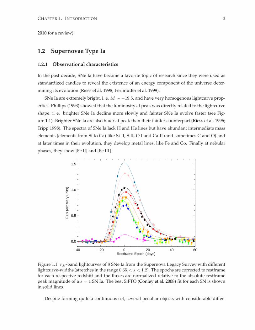
SNe Ia are extremely bright, i. e. M ∼ −19.5, and have very homogenous lightcurve prop-
erties. Phillips (1993) showed that the luminosity at peak was directly related to the lightcurve
shape, i. e. brighter SNe Ia decline more slowly and fainter SNe Ia evolve faster (see Fig-
ure 1.1). Brighter SNe Ia are also bluer at peak than their fainter counterpart (Riess et al. 1996;
Tripp 1998). The spectra of SNe Ia lack H and He lines but have abundant intermediate mass
elements (elements from Si to Ca) like Si II, S II, O I and Ca II (and sometimes C and O) and
at later times in their evolution, they develop metal lines, like Fe and Co. Finally at nebular
phases, they show [Fe II] and [Fe III].
−40 −20 0 20 40 60Restframe Epoch (days)
0.0
0.5
1.0
1.5
Flu
x (a
rbitr
ary
units
)
Figure 1.1: rM -band lightcurves of 8 SNe Ia from the Supernova Legacy Survey with differentlightcurve-widths (stretches in the range 0.65 < s < 1.2). The epochs are corrected to restframefor each respective redshift and the fluxes are normalized relative to the absolute restframepeak magnitude of a s = 1 SN Ia. The best SiFTO (Conley et al. 2008) fit for each SN is shownin solid lines.
Despite forming quite a continuous set, several peculiar objects with considerable differ-

CHAPTER 1. INTRODUCTION 4
ences have been found in the past. On the bright extreme, there is the group of slow declining
objects similar to SN1991T (Filippenko et al. 1992a; Ruiz-Lapuente et al. 1992; Phillips et al.
1992; Jeffery et al. 1992; Spyromilio et al. 1992). On the faint end, the group of intrinsically red
and fast decliners like SN1991bg (Leibundgut et al. 1993; Filippenko et al. 1992b; Turatto et al.
1996) have strong Ti II and enhanced Si II lines in their spectra. Other atypical SNe Ia consist of
SN2000cx (Li et al. 2001b; Candia et al. 2003) and SN2002cx-like objects (Li et al. 2003), similar
in the pre-maximum spectra to SN1991T but evolving fast, and as faint as SN1991bg.
SNe Ia are found in every type of galaxy, in spirals and ellipticals, and are therefore not
uniquely associated with star forming regions. Interestingly, the stellar environment of SNe Ia
is related to their intrinsic properties. Bright and slow decliners occur in regions associated
with star formation, where they are more common (Mannucci et al. 2005; Sullivan et al. 2006b),
while fainter and faster SNe Ia prefer passive or elliptical host galaxies (Hamuy et al. 1995,
1996c; Riess et al. 1999a; Hamuy et al. 2000; Sullivan et al. 2006b; Aubourg et al. 2008). These
environmental effects are reproduced in the spectra as well: SNe Ia in late-type galaxies show
weaker lines of intermediate mass elements than in early-type galaxies (Bronder et al. 2008;
Balland et al. 2009; Sullivan et al. 2009). Studies of the metallicity environment of SN Ia reveals
a much weaker relation with SN properties than the stellar age (Gallagher et al. 2008; Howell
et al. 2009).
As will be shown in next section, different progenitor scenarios predict different delay
times from the birth of the binary system to the explosion of a SN Ia. Exploring the delay time
distribution (DTD) of SNe Ia helps constraining progenitors. This has been done comparing
the SN Ia birthrate to the cosmic star formation (e. g. Gal-Yam & Maoz 2004; Strolger et al.
2004; Scannapieco & Bildsten 2005; Mannucci et al. 2006; Pritchet et al. 2008; Maoz et al. 2011),
or directly constructing it from the age of the stellar populations through detailed host galaxy
photometry and spectroscopy (Totani et al. 2008). Furthermore, as SNe Ia are a source of iron-
peak elements3 into the intergalactic medium, the SN Ia birthrate is related to the cluster iron
abundance (e. g. Matteucci et al. 2006) and the latter can be used as an additional constraint to
normalize DTDs (Maoz et al. 2010). The latest DTD results, including estimates from the rate
of SN Ia remnants (Maoz & Badenes 2010), are converging to a power-law DTD that scales
inversely with cosmic time, t−1.
1.2.2 Explosion and Progenitor scenarios
Due to their occurrence in every galaxy –particularly in old stellar populations– and the ab-
sence of hydrogen and helium in their spectra, SNe Ia are believed to originate from long-lived
3Elements and isotopes close to the iron nuclear binding energy peak: vanadium, chromium, manganese, iron,cobalt, and nickel

CHAPTER 1. INTRODUCTION 5
low-mass stars, MZAMS < 8M⊙4, that end up their lives as carbon-oxygen white dwarfs (CO-
WDs), with a mass distribution peaking at M ≃ 0.6M⊙, well below the Chandrasekhar limit5.
If they happen to be in a binary system, where mass can be accreted into the WD nearing the
Chandrasekhar limit or causing enough compressional heating, then the C/O material can be
ignited. As the WD is degenerate, this burning becomes explosive and rapidly disrupts the
entire star. Iron-peak and intermediate-mass elements synthesized in the process are ejected
at high velocities to space and no compact remnant is left behind. The kinetic energy of a SN Ia
is approximately equal to the difference of the thermonuclear burning of aWD and its binding
energy.
The lightcurve of a SN Ia is powered by the radioactive beta decay of 56Ni to 56Co and
then to 56Fe (Truran et al. 1967; Colgate & McKee 1969; Arnett 1982), which releases large
quantities of gamma rays thermalized to the optical regime. At peak, most of the light is in
the visible and some in the near-ultraviolet (NUV) and near-infrared (NIR). The rise to peak
lasts 10-24 days depending on the SN Ia and, once the radioactive energy released equals the
radiated luminosity, the luminosity starts decreasing. Due to a long diffusion time of photons,
at early times the outer layers of the SN are seen, while the inner products of the explosion
appear in the spectra later in time, as the photosphere recedes. Near peak, the spectra show P-
Cygni profiles, weeks later they show scattering lines, and finally emission lines in the nebular
phase6, as the photosphere becomes optically thin (Branch et al. 2006). Much later (hundreds of
days), gamma rays from the decay of 56Co can freely escape and the lightcurve slope resembles
the radioactive decay, as long as positrons are trapped (Lair et al. 2006), and spectral lines show
iron-peak elements from the innermost parts of the explosion.
Although consensus exists on the general features, the exact details of the WD progenitor,
especially the companion, as well as the detailed physics of the explosion are subject to vigor-
ous debate. The theoretical models need to explain the abundant observations of SNe Ia and
the relations binding these together. Currently, three main progenitor scenarios are discussed:
Single Degenerate: The single degenerate (SD) scenario, a favored scenario in the past, sug-
gests an evolved or main sequence companion (Whelan & Iben 1973) donating material
to the WD nearing the Chandrasekhar limit. The rate of the accretion needs to be steady,
between 107 − 108M⊙yr−1 (Nomoto 1982) to avoid novae and mass loss (slower accre-
tion), or expansion into a giant envelope (higher accretion). The most viable candidates
4The zero age main sequence mass, MZAMS refers to the mass of a star at the onset of H core fusion in the mainsequence
5The Chandrasekhar limit (Chandrasekhar 1931) refers to the maximum mass above which a white dwarf’selectron degeneracy pressure is unable to sustain the self-gravity of the star. It is close to 1.4M⊙.
6The nebular phase occurs when the ejecta is optically thin to continuum photons. These come from convertedgamma rays of 56Co decay and are seen as emission lines in the spectra

CHAPTER 1. INTRODUCTION 6
of such binary systems are supersoft X-ray sources (Rappaport et al. 1994), although their
observed rate in the Milky Way and other galaxies seem to account for only ∼ 5% of the
SN Ia rate (Di Stefano 2010a; Gilfanov & Bogdan 2010).
The main argument against the accretion from a non-degenerate companion is the lack
of hydrogen seen in SNe Ia (Leonard 2007). The outer layers of the companion during
Roche lobe overflow are stripped and become part of the SN ejecta, making them visible.
Symbiotic channels (e. g. Hachisu et al. 1996), where the WD accretes mass from the stel-
lar wind of the companion, try to bypass this issue, but the absence of radio signatures
for SNe Ia sets a limit of steadymass loss prior to the SN that disfavors such mechanisms
(Panagia et al. 2006).
Moreover, the occurrence of super-Chandrasekhar SNe Ia, explosions that seem to re-
quire WDs of masses exceeding the Chandrasekhar limit (e. g. Howell et al. 2006; Hicken
et al. 2007; Scalzo et al. 2010; Yuan et al. 2010), are also at odds with the slow accretion
near MCh required by the SD scenario (although see Hachisu et al. 2011).
Additionally, although the number of WDs in close binaries with non-degenerate com-
panions is sufficient to explain the SN Ia birthrate, the predicted DTDs (Yungelson &
Livio 2000; Greggio 2005; Mennekens et al. 2010) do not agree with the recent empirical
DTDs (Totani et al. 2008; Maoz et al. 2010; Graur et al. 2011), i. e. they do not have a
power-law with steeper index than −1.
Furthermore, a red giant companion as themain channel is currently disfavored as recent
well sampled early lightcurves (Hayden et al. 2010a; Bianco et al. 2011) do not show any
evidence for a hole left by the companion in the early-time supernova ejecta (Kasen 2010).
Some of these criticisms, like lack of H and no signature of a companion during the
rise, have been addressed with more exotic SD theories, like the scenario proposed by
Justham (2011), where the WD gains angular momentum that stabilizes it and prevents
ignition until the H-rich envelope of the donor is exhausted and contracts, leaving the
WD in a wide orbit binary before explosion.
Double Degenerate: The double degenerate (DD) scenario consists of twoCO-WDs thatmerge
together to reach the Chandrasekhar mass (Iben & Tutukov 1984; Webbink 1984). An ac-
cretion disk from the disruptedWD forms around the more massive primary and carbon
is ignited on the surface.
One of the main drawbacks of the DD scenario is that such a burning is non-explosive
and will lead to a ONe-WD that ultimately collapses to a neutron star (Saio & Nomoto
1985), although this might be prevented under some assumptions (Yoon et al. 2007). Cur-

CHAPTER 1. INTRODUCTION 7
rent models of WD mergers are able to produce only subluminous SNe Ia (Pakmor et al.
2010) and more three-dimensional simulations need to investigate this intricate process
further. The DD scenario also suffers from a lower observed rate of X-ray emission in
nearby galaxies compared to predictions of supersoft X-ray binaries, supposed transi-
tion states of DD progenitors (Di Stefano 2010b), but this discrepancy is lower than for
the SD scenario.
On the other hand, the DD channel naturally explains the absence of H, it agrees well
with the empirical relative DTDs obtained from the SN Ia birthrates (Totani et al. 2008;
Maoz et al. 2011; Graur et al. 2011), it satisfies the non-observation of a companion sig-
nature in early rise-time studies, and it can also better account for super-Chandrasekhar
SNe Ia from the merger of two WDs whose total mass exceeds the limit.
Additionally, in this framework, the relation between SN Ia properties and stellar en-
vironments seems naturally explained: brighter SNe Ia occur in younger populations
where more massive WDs merge, whereas fainter SNe Ia come from less massive WD
progenitors, characteristic of older populations.
The only observational weakness is that the predicted rate (or absolute DTDs) is higher
than the observed one (Maoz et al. 2010), that is, there are not enoughWDbinary systems
exceeding the Chandrasekhar limit.
Sub-Chandrasekhar: Explosions of WDs below the Chandrasekhar mass have recently been
revived. In the previous two scenarios, the WD explodes near the Chandrasekhar mass.
Such an explosion cannot be explained by a pure detonation7 since the high density of
the burning produces too many iron-peak elements and few intermediate mass elements
(Arnett 1969). A pure deflagration8, on the other hand, cannot account for the high ve-
locities of the outer ejecta (Mazzali et al. 2005). The favored mechanism is therefore a
transitional combustion starting with a subsonic deflagration leading to a supersonic
detonation (Khokhlov 1991). The physics of the transition are not well understood but
the lightcurve, spectra, and lightcurve width-luminosity relation of SNe Ia are well recre-
ated (Kasen et al. 2009).
Instead of adding a somewhat unnatural deflagration-to-detonation transition, a sub-
Chandrasekhar detonation of a WD with lower mass and density can naturally produce
the right mix of iron peak and intermediate mass elements. Furthermore, it could also
explain the lower empirical ejecta masses of some SNe Ia (Stritzinger et al. 2006). Simu-
lations (Sim et al. 2010) show that the detonations of sub-Chandrasekhar mass WDs can
7A detonation is a supersonic combustion propagating through shock compression8A deflagration is a subsonic combustion propagating though the transfer of thermal energy
CHAPTER 1. INTRODUCTION 8
reproduce lightcurves and spectra of SNe Ia.
The problem lies in the right trigger for carbon ignition. The original models (Woosley
& Weaver 1986) had an initial layer of accreted helium detonating and creating a shock
wave towards the core of the WD that would generate a second detonation propagat-
ing outwards and disrupting the WD. These models were rejected because of the large
amount of 56Ni generated in the early portion of the lightcurve from the He-burning,
which is inconsistent with observations (Nugent et al. 1997). Nowadays. indications ex-
ist that He can detonate in amuch thinner layer (Shen et al. 2010), allowing the possibility
for such a double detonation. This channel requires further theoretical development to
explore if it can confirm diverse aspects of SNe Ia observables.
Of particular interest in sub-Chandrasekhar models are the merger of CO-WDs below
the Chandrasekhar limit. All the benefits of the DD scenario, such as the lack of H, the
relative DTD and the early rise time behavior, are inherited. Additionally, the proper
fraction of binary systems leading to explosions, and with it the absolute DTD, are ob-
tained, since lower-mass WDs, which are more frequent, can merge and explode as
SNe Ia. However, Loren-Aguilar et al. (2009) and Pakmor et al. (2010) show that the
merger of two CO-WDs of equal mass below ∼ 0.9M⊙ are not hot enough to ignite C
in the core. Moreover, due to the low central density of the WD, the only successful
explosions that are achieved are subluminous ones. Ideas to circumvent this are com-
pressional heating from a thick accretion disk around the rotating WD after the merger
(van Kerkwijk et al. 2010), although full simulations are required to test the viability
of this channel. If some sort of heating mechanism extends over all WD mass ranges,
super-Chandrasekhar models could also be explained, as in the regular DD scenario.
The last years of SN Ia science has led to a shift in the favored progenitor channel away
from the SD scenario. The DD channel and the recently revived sub-Chandrasekhar models
are promising candidates, although clearly more extensive multi-dimensional simulations are
required to test how feasible they are. Evidently, SNe Ia can originate via multiple channels,
and the different scenarios could each play a contributing role.
1.2.3 SNe Ia as distance indicators
Correcting for the empirical relations of lightcurve width-luminosity and color-luminosity
makes SNe Ia good standard candles, providing direct evidence for an unknown dark energy
driving the accelerated expansion of the universe (Riess et al. 1998; Perlmutter et al. 1999).
Additional relations with luminosity have been searched for to further improve SNe Ia as
distance rulers. A third parameter has recently been introduced relating luminosity to host

CHAPTER 1. INTRODUCTION 9
environment, i. e. brighter SNe Ia occur in more massive host galaxies (Sullivan et al. 2010;
Kelly et al. 2010; Lampeitl et al. 2010). Other possible corrections include metallicity (e. g.
Timmes et al. 2003; Gallagher et al. 2005; Howell et al. 2009; Yasuda & Fukugita 2010), spectral
features such as high-velocity lines (Wang et al. 2009a) or flux ratios (Bailey et al. 2009; Yu et al.
2009).
Current SN Ia cosmological studies (e. g. Kessler et al. 2009; Conley et al. 2011) (see Fig-
ure 1.2) have reached a mature state where the systematic uncertainties are comparable to
statistical uncertainties directly affecting the measurement of the dark energy’s equation of
state, w. The present and future challenges of supernova cosmology thus reside in under-
standing and diminishing those systematic biases. Here is a brief summary of those (for a
more complete description, see Conley et al. 2011).
Figure 1.2: Hubble diagram of combined SNe from different samples (low-z, SDSS, SNLS andHST). The bottom plot shows the residuals from the best fit for a falt universe: Ωm = 0.18±0.10and w = −0.91+0.17
−0.24. From Conley et al. (2011)
Calibration: The current most important systematic by far is the calibration across SN sam-
ples at different redshifts. As SNe at higher-z are redshifted and other bandpass filter
are used, different samples need to be converted to a common standard photometric
system, and relative fluxes need to be calculated. This permits the direct comparison of
SNe at different redshifts. Most of the low-z dataset is currently on the Landolt system
(Landolt 1992), which is not well understood. Thus, the calibration systematic will be
substantially reduced once different high-z SN samples are cross calibrated to the low-z

CHAPTER 1. INTRODUCTION 10
SN sample, or new low-z data in better understood systems become available (like the
SNfactory –Bailey et al. 2009, CSP –Folatelli et al. 2010 and more SDSS-II –Kessler et al.
2009).
Lightcurve-fitter: Another smaller systematic arises from the fitter used to parameterize the
SN lightcurve shape, that serves later to correct each SN’s luminosity. There are clear
differences in the SN color treatment of fitters like SALT2 (Guy et al. 2007) and SiFTO
(Conley et al. 2008) versus fitters like MLCS2k2 (Jha et al. 2007). Particularly, fitters
trained with low-z data exclusively, like MLCS2k2, suffer from missing rest-frame U -
band data which becomes important at high-z, where redshifted SNe are probed in that
wavelength regime. Differences from various fitters represent another relevant system-
atic contributing to SN cosmology (Guy et al. 2010).
Reddening: An important systematic and elusive concern in SN Ia cosmology has been the
color/dust degeneracy. Corrected for in the color-luminosity relation entering the resid-
uals of the Hubble diagram, the SN color has been difficult to disentangle from dust in
the line of sight. The reddening law inferred from SNe is significantly different from the
Milky Way dust (lower RV9). This may be due to the mix of intrinsic SN reddening and
dust, or alternatively it can be caused by a different dust in the line of sight to SNe Ia or
scattering effects from circumstellar material (Wang 2005; Goobar 2008).
Local NIR observations benefit from less sensitivity to dust and help characterize the in-
trinsic colors of SNe Ia. Althoughwith low statistics, using ratios of color excesses in the
optical and NIR, Folatelli et al. (2010) find an indication that low-extincted SNe Ia have
a reddening law like the Milky Way’s, while redder objects follow a different one (lower
RV ). Furthermore, spectral studies show that SNe Ia of different velocity gradients may
have varying colors and RV (Pignata et al. 2008; Wang et al. 2009a). This would mean
that there is an intrinsic color variation of SNe Ia that correlates with luminosity but in-
dependent of the SN properties, such as lightcurve-shape. This could imply different
progenitor scenarios leading to SNe of different velocities and different color properties.
Observations of the correlation of the late nebular emission lines with SN color suggest
that this diversity of SNe Ia could come from varying observing angles of asymmetric
explosions (Maeda et al. 2011).
In the latter cases, the need for a separate correction for intrinsic SN color and dust red-
dening for cosmological studies seems necessary. Some attempts to account for this have
been made (Sullivan et al. 2010; Lampeitl et al. 2010) by dividing the SN set according to
9RV is a parameter describing the extinction curve of interstellar dust and is defined as AV /EB−V , withEB−V = AB − AV , where AB and AV are the total extinctions in B and V bands.

CHAPTER 1. INTRODUCTION 11
their host properties, like star formation, and applying an independent reddening cor-
rection for each subset. Such exercises reveal differences in the reddening laws: a lower
RV is found for hosts with lower star formation.
Finally, in contrast to the traditional B-band Hubble diagrams, the restframe IR Hubble
diagrams (Krisciunas et al. 2004a; Wood-Vasey et al. 2008; Freedman et al. 2009) offer an
interesting new approach to cosmology with SNe Ia that has less reddening bias and a
tighter dispersion, even without a lightcurve shape correction.
Evolution: A long lasting concern for cosmology resides in the possible evolution of SNe Ia
and SN Ia populations as a function of cosmic time. This is an extremely important
matter that suffers from a poor understanding of the physics of the progenitors and ex-
plosions of SNe Ia. The evolution of the demographics of SNe Ia is a known effect seen to
z ≃ 1 (Howell et al. 2007). Since brighter SNe Ia occur only in late-type galaxies whereas
fainter ones are found in both, elliptical and spiral galaxies, the population of SNe Ia
observed at different lookback times will change as the cosmic star formation increases
with redshift. This change in population does not affect the cosmological studies since
SNe Ia are corrected for the lightcurve-width relation to the same absolute magnitude.
On the other hand, evolutionary changes in this relation itself (through changes in the
α parameter) will be of greater concern, but studies show no conclusive evolution (Guy
et al. 2010).
Moreover, claims of an evolving intergalactic gray dust making SNe fainter without red-
dening them, have stood in opposition to the acceleration of the universe since its pro-
posal (Aguirre 1999) and continue today (Corasaniti 2006; Bogomazov & Tutukov 2011).
Regular intergalactic dust evolution (Menard et al. 2010) has been shown to represent
only a small systematic, and reddening evolution remains marginal (studied through
changes in the β parameter of the luminosity-color relation) (Guy et al. 2010; Conley
et al. 2011), despite some claims (Kessler et al. 2009).
Others: Additional systematic uncertainties affecting cosmological studies to a lesser extent
include uncertainties in theMalmquist bias corrections10; uncertainties in theMilkyWay
extinction correction (Schlegel et al. 1998); the adopted local flow model, or nearby pe-
culiar velocities; contamination from non-Ia SNe; and gravitational lensing effects (Holz
& Linder 2005; Jonsson et al. 2010).
10The Malmquist bias is a selection bias to preferentially detect brighter objects

CHAPTER 1. INTRODUCTION 12
1.3 Core-collapse supernovae
1.3.1 Observational characteristics
Core-collapse SNe are a heterogeneous set with different spectral and lightcurve features. SNe
of type Ib/c lack hydrogen in their spectra. SNe Ib do not possess Si II lines but have He I,
whereas SNe Ic do not show helium either. Both, SNe Ib and SNe Ic, show lines of Ca II, O I,
Na I, Fe II, Ti II in photospheric phase and [O I] and [Ca II] in the nebular phase (Millard et al.
1999; Matheson et al. 2001; Branch et al. 2002). SNe Ibc are on average fainter than SNe Ia, i. e.
MB ∼ −18 at peak with a larger dispersion (Richardson et al. 2002).
SNe II are characterized by the presence of hydrogen lines in their spectra. The observed
lightcurve display varies widely. Plateau supernovae (IIP) show a plateau phase after max-
imum, where the luminosity remains almost constant for 80-150 days. The peak brightness
is on average MB ∼ −17 with a large dispersion (Richardson et al. 2002). Type II linear SNe
(IIL) are brighter than SNe IIP (similar to the brightness of SNe Ibc) and show a steady de-
cline in luminosity after maximum. Narrow-lined SNe (IIn) have dominant narrow emission
lines (Schlegel 1990) from interaction of the ejecta with circumstellar material (CSM). They also
show He I emission lines, Balmer and Na I absorption lines. The CSM creates inner and outer
shocks as the ejecta interacts with it and makes the lightcurve very bright for several years.
Variations in the amount and density of the CSM give rise to quite a heterogeneous sample.
Finally, SNe IIb are a transitional case, in which spectra resemble SNe II at early times but later
evolve SN Ibc features (Filippenko et al. 1990).
The tail of the lightcurve of CC SNe is powered by the radioactive decay of 0.1M⊙ of 56Ni
synthesized and ejected by the explosion, as it transitions first to 56Co and then to 56Fe . In
type Ib/c, where the H-envelope is absent, the 56Co decay powers almost the entire display
and no plateau is seen. In SNe IIL, where a good portion of the H-envelope was lost but not
all, a small plateau merges into the 56Co powered tail so that a “linear” decline is observed.
CC SNe are characterized by their occurrence in regions of active star formation. They
have been mainly observed in disks and spiral structures of late-type galaxies (e. g. Johnson
& MacLeod 1963; Maza & van den Bergh 1976; Barbon et al. 1999), they are commonly found
in OB-associations and H II regions (Bartunov et al. 1994; van Dyk et al. 1996; Tsvetkov et al.
2001), and they follow the radial distribution of Hα emission (Anderson & James 2009). Addi-
tionally, the CC-SN rate traces the cosmic star formation rate (Cappellaro et al. 1999; Mannucci
et al. 2005; Dahlen et al. 2004; Botticella et al. 2008; Bazin et al. 2009; Graur et al. 2011). More-
over, differences in the radial distributions and concentrations among the SN subtypes point
towards a progenitor mass and metallicity dependence (Anderson & James 2008; Kelly et al.
2008; Prieto et al. 2008; Hakobyan et al. 2009; Boissier & Prantzos 2009; Habergham et al. 2010;

CHAPTER 1. INTRODUCTION 13
−50 0 50 100 150Restframe Epoch (days)
0.0
0.5
1.0
1.5
Flu
x (a
rbitr
ary
units
)
IIPIbcIIn
Figure 1.3: rM -band lightcurves of 3 CC SNe from the Supernova Legacy Survey: IIP (pinkdots), IIn (green dots) and Ibc (blue dots). The epochs are corrected to restframe for eachrespective redshift and the fluxes are normalized relative to an absolute magnitude of −16.0.
Modjaz et al. 2011): SNe Ibc are more related to the bright, metal-rich regions of their host
galaxies and follow the H II regions more closely than SNe II, and SNe Ic even more so than
Ib.
The study of the copious neutrino emission of CC SNe, as seen for SN1987A (Bionta
et al. 1987; Hirata et al. 1987), is of great importance for understanding the explosion mecha-
nism and has opened up exciting possibilities for promising underground observatories (e. g.
Koshiba 1992; Ewan 1992). Also, the study of the compact remnants left after the explosion,
i. e., the neutron stars (NS), gives valuable insight into the physics of the explosion. Their ve-
locities, or “kicks”, for instance reveal that the explosion is asymmetrical (Cordes et al. 1993;
Lyne & Lorimer 1994). The shape of supernova remnants, line profile studies (Wooden et al.
1993) and polarization measurements (Wang et al. 1997) confirm this.
1.3.2 Theory of explosion
Core-collapse SNe originate from massive stars (MZAMS & 8M⊙) that undergo core collapse
after they have exhausted their iron fusion supply, only a 4-40 million years after being born.
Massive stars have a complex evolution (see Woosley et al. 2002 for a review) where nuclear
fusion of higher mass elements occurs one after the other until a final iron core is produced.
At this stage, no net energy can be produced and an electron degeneracy builds up that cannot
halt the implosion as the mass of the iron core reaches the Chandrasekhar limit. The outer

CHAPTER 1. INTRODUCTION 14
part of the core collapses rapidly (23% of light velocity in some milliseconds) due to its own
gravity producing high-energy gamma rays that photo-dissociate iron nuclei into neutrons
and α particles. Further neutrons and neutrinos are created as the core density increases and
electrons are captured. The collapse is eventually stopped by neutron degeneracy and matter
rebounds in a shock wave propagating outwards (Bethe et al. 1979). The shock wave dissoci-
ates elements in the core losing energy and starts to stall. At this point, a new energy source,
like escaping neutrinos for example, is believed to power the explosion and blast the outer
layers away. The collapse results in a compact object such as a neutron star or a black hole,
depending on the initial mass of the star (Baade & Zwicky 1934). The rapidly expanding ejecta
form then a supernova remnant that enriches the interstellar medium with heavy elements
produced in the star and the explosion. This will later be used for a new generation of young
stars that have more metals shaping ultimately the chemical evolution of galaxies.
This summarized picture of a core-collapse triggering a SN does not describe the detailed
mechanism of the explosion. As a matter of fact, the initial shock needs to propagate through
infalling material. The energy loss through dissociation of heavy nuclei and enormous neu-
trino luminosities created by electron capture stalls the shock, as shown in multiple simula-
tions (e. g. Bruenn 1985; Wilson et al. 1986; Myra & Bludman 1989; Mezzacappa et al. 2001;
Liebendorfer et al. 2001; Buras et al. 2003; Janka et al. 2004). This important issue is solved
via the favorite mechanism of neutrino heating (e. g. Bethe & Wilson 1985; Wilson & Mayle
1988; Herant et al. 1994), in which neutrinos of all flavours from the nascent accreting neutron
star in the center, that were initially trapped (due to mean free paths shorter that the star ra-
dius) diffuse out in a split second (Burrows 1990), and release their high degeneracy energy
into thermal energy (Burrows & Lattimer 1986; Burrows 1988). In this way, the stalled shock
gains energy deposited by a fraction of the escaping neutrinos in the region between the proto-
neutron star and the stalled shock (Mayle & Wilson 1988; Burrows & Goshy 1993; Janka 2001).
In multiple dimensions, simulations of the neutrino-driven explosion are accomplished with
help of the advective-acoustic Standing-Accretion-Shock-Instability (SASI) (Foglizzo & Tagger
2000; Blondin et al. 2003). Alternative mechanisms to revive the stalled shock exist and include
the acoustic power generated by core pulsations, proposed by Burrows et al. (2006).
The total energy liberated by the explosion is around 1053ergs, most of it as neutrinos. The
shock wave generated in the collapse is visible in UV after a few hours, once it reaches the
surface of the star. The energy deposited by the shock in the envelope powers the lightcurve
after peak maximum (and some decay energy of 56Ni ). This energy diffuses out and keeps the
envelope hot and the Hydrogen ionized. Depending on the envelope, a Hydrogen recombina-
tion wave propagates inward in mass (and velocity). The plateau of SNe IIP is explained by
such hydrogen recombination of a large envelope at around T ≃ 5500K that releases trapped

CHAPTER 1. INTRODUCTION 15
radiation. Other CC SNe have less or no hydrogen layers, reducing the optical display. The
decay of 56Ni synthesized in the explosion powers the late time SN lightcurve. This exponen-
tial decline can be affected by dust formation that absorbs and re-emits light in the IR, so that
the optical lightcurve decreases more rapidly. In some cases, the late recombination of ionized
elements in the explosion can occur at epochs longer than the time of expansion of the SN
(Leibundgut & Suntzeff 2003).
1.3.3 Progenitor scenarios
The wide variety of CC SNe, including radiated energy, chemical composition and kinetic
energy, reflects a diverse range of progenitor properties affecting the output: mass, metallicity,
binarity, mass-loss rate, rotation and magnetic activity (Podsiadlowski et al. 1992; Heger &
Langer 2000; Hirschi et al. 2004; Yoon & Langer 2005).
According to theoretical models, the progenitors of SNe II are massive stars that retain
the hydrogen envelopes (e. g. Woosley & Weaver 1986; Hamuy 2003). SNe IIP are believed
to come from red supergiants (RSG) in the lower mass range of CC SNe (8 − 20M⊙). SNe
IIL have lost some of their H-envelope (they have less than ∼ 2M⊙ of H) and have higher
mass progenitors, possibly early B stars (or alternatively are the result of a collapsing 8M⊙ <
M < 10M⊙ ONeMg-WD). SNe IIb have even less hydrogen and presumably more massive
progenitors.
SNe Ibc originate either from massive O stars that lose their hydrogen layers (and helium
in some cases) by strong stellar winds, as predicted for Wolf-Rayet stars (WR) (SNe Ib would
come fromWN stars, WR stars with strong nitrogen emission lines, and SNe Ic fromWC/WO
stars,WR stars with dominant carbon/oxygen emission lines from the inner parts of a stripped
star) with main sequence masses of & 25 − 30M⊙ (e. g. Woosley et al. 1993; Heger et al. 2003;
Maeder & Meynet 2004), or they come from lower mass stars that lose their envelopes though
stripping from mass transfer in a binary system (e. g. Podsiadlowski et al. 2004a; Eldridge &
Tout 2004), or a combination of both processes.
Therefore, the sequence of increasing hydrogen abundance and decreasing mass stripping
for CC SNe is: Ic-Ib-IIb-IIL-IIP. Understanding the origin of this sequence is a key feature to
progenitors. The other important element is the presence of circumstellar material interacting
with the SN ejecta. The clearest of these is the SN IIn category, but objects of other types also
show evidence of some interaction, like SNe IIL and IIP, and even possibly SNe Ia (e. g. Benetti
et al. 1998; Sollerman et al. 1998; Turatto et al. 2000; Hamuy et al. 2003). Depending on the
CSM density, its location and extent, as well as the velocity of the ejecta, the interaction will be
different and the lightcurve as well. The CSM will often come from previous episodes of mass
loss of the progenitor stars.

CHAPTER 1. INTRODUCTION 16
The most direct way to probe progenitors is to look for them in pre-explosion images (e. g.
Van Dyk et al. 2003; Smartt et al. 2004; Maund & Smartt 2005; Li et al. 2006b; Mattila et al.
2008; Leonard et al. 2008). Smartt et al. (2009) group those observations into a volume-limited
sample and conclude with a maximum likelihood analysis that, for a Salpeter IMF11, the pro-
genitors of SNe IIP have a minimum mass of 8.5 ± 1M⊙ and a maximum allowed mass of
∼ 16M⊙. The lack of progenitors with larger masses, beyond 17M⊙, poses a challenge to pre-
vious theoretical models and suggest that these stars explode in other forms: IIL, IIn and Ibc
SNe. This could mean that mass loss is more important than previously thought or that stellar
metallicities were underestimated. Alternatively, RSG stars above this mass could end their
lives in a direct black hole formation with extremely weak explosions (Fryer 1999; Heger et al.
2003).
The discovery of SNe Ibc progenitors through pre-explosion images has been inconclusive
despite different attempts (e. g. Maund & Smartt 2005; Crockett et al. 2007). The non-detection
however argues for another progenitor channel besides the WR stars, lower mass stars in
interacting binaries (Smartt 2009). Furthermore, WR stars have masses larger than & 25M⊙
(Massey 2003; Crowther 2007), which is not enough to account for the high estimated Ibc
fractions (Smartt et al. 2009; Li et al. 2010a). Additionally, the observed ratio of WC/WN,
which ranges between ∼ 0.1 − 1.2 for different metallicities, as compared to the Ic/Ib ratio
of ∼ 2, suggests that binary interactions play a significant role (or that the WN stage is only
a momentary phase in the evolution of WR stars). Finally, some SNe Ic of low energy have
Carbon and Oxygen remnant masses that are much smaller than the observed masses of CO
cores of WC stars (Crowther et al. 2002), an observation that argues that these stars are the
outcome of interactions of lower mass stars in binary systems.
On the contrary, comprehensive recent environmental studiesmentioned in $ 1.3.1 indicate
a sequence in the progenitor masses of CC SNe: II-Ib-Ic. This supports the idea that strong
stellar winds strip the envelopes of massive single stars that collapse later in big SN displays.
Nonetheless, the regions of high SN Ibc concentration also show a higher stellar density (Clark
et al. 2008), and therefore a higher binary fraction, possibly leading to more frequent binary
interactions and mergers that could contribute to this enhancement (Portegies Zwart et al.
2010). The most probable explanation is that both channels, single and binaries, contribute to
SNe Ibc, although the exact fraction and extent of each remain to be found.
Lastly, it is worth to mention that some SNe Ic have also been associated to long-duration
Gamma Ray Bursts (LGRBs) (e. g. Mazzali et al. 2006; Valenti et al. 2008). These SNe Ic have
broad line widths (∼ 30000km/s) (e. g. Galama et al. 1998; Patat et al. 2001; Pian et al. 2006).
11The Initial Mass Function (IMF) is the empirical distribution of initial star masses. The Salpeter IMF (Salpeter1955) has the shape M−α with slope α = 2.35.

CHAPTER 1. INTRODUCTION 17
The energetic jets may be powered by a central engine such as the newly formed and highly
magnetized neutron star (magnetar) (e. g. Wheeler et al. 2000; Lyutikov & Blackman 2001;
Drenkhahn & Spruit 2002) or a black hole with a rapidly rotating disk (collapsar) (Woosley
1993; MacFadyen & Woosley 1999). Not all WR stars (with MZAMS > 40M⊙) produce broad-
line SNe Ic since their fraction is much larger than the rate of broad-line SNe Ic (Podsiadlowski
et al. 2004b). There is evidence that broad-line SNe Ic have different metallicities than normal
SNe Ic arguing for a different progenitor (Modjaz 2011).
1.3.4 SNe IIP as distance indicators
Although they are intrinsically fainter than SNe Ia, SNe IIP represent the most homogeneous
set of core-collapse SNe (Hamuy 2003) and their use as independent cosmological distance
indicators has been demonstrated. There exist some theoretical-driven methods to calculate
the distance such as the expanding photosphere method (Kirshner & Kwan 1974; Schmidt
et al. 1994a; Hamuy et al. 2001) or the synthetic spectral fitting expanding atmosphere method
(Baron et al. 2004; Dessart et al. 2008). An empirical simpler method, the standardized candle
method, relies on the correlation between the expansion velocity and the brightness of SNe IIP
during their plateau phase (Hamuy & Pinto 2002). The origin of this relation can be physically
explained by the fact that more luminous SNe will have a hydrogen recombination wave at
larger radii than fainter SNe, so that the velocity of the photosphere will also be greater (in
a homologous expansion: v ∝ r). Nugent et al. (2006) improved this method to moderate
redshifts (z ∼ 0.3) by adding an extinction correction based on the V − I colors at day 50 after
maximum. Other nearby studies of the standardized candle method for SNe IIP like Poznanski
et al. (2009); Olivares (2008) and D’Andrea et al. (2010) for the SDSS, have increased the sample
testing the validity of the method for a larger number of objects. The distance scatter oscillates
between 10 and 18%.
Furthermore, NIR photometry can potentially improve the use of SNe IIP as standardiz-
able candles. As dust causes less extinction in these bands, one should expect more precise
Hubble diagrams. Maguire et al. (2010) present a local NIR Hubble diagram for SNe IIP with
lower scatter than for optical bands (for the same SNe) although a larger sample is needed to
confirm their results. Further studies of SNe IIP at low-z (ideally with IR data) should help
understand the SN IIP properties and their standardizable capabilities better, so that future
facilities can use the information to the SN IIP datasets that will be discovered at cosmological
redshifts. SNe IIP have different and better understood progenitors than SNe Ia, and provide
a promising independent cosmological probe.

CHAPTER 1. INTRODUCTION 18
1.4 Motivation for this dissertation
The development of more powerful technologies to discover and characterize supernovae in
the past years has revolutionized the field. The Supernova Legacy Survey (SNLS) has been
fundamental in expanding our understanding of supernovae and their use for cosmology.
With the aim of pinpointing the dark energy of the universe with greater accuracy, its rolling
search strategy discovered more than ∼ 500 spectroscopically confirmed SNe Ia in the inter-
mediate redshift regime of 0.1 < z < 1.1, during its five years of activity.
The SNLS has been incredibly successful at its goal (Astier et al. 2006; Guy et al. 2010; Con-
ley et al. 2011; Sullivan et al. 2011a) and has contributed to achieve a new era of SN cosmology
in which systematic errors are of the order of statistical errors. A real further improvement
can only be attained by fully understanding the nature and extent of these systematic effects.
In this process, the real challenge resides in finally grasping the nature of SN Ia progenitors
and explosions. As long as the fundamental answers of SNe Ia remain elusive to us, the quest
for the essence of the dark energy will not be satisfied. Currently, as previously shown, the
largest systematic are the ones that we understand best and that are associated to observa-
tional effects. It is possible that as we find out more about SNe Ia, the main systematics may
shift towards yet unknown biases of their explosions and evolution.
Numerous scientific studies of the SNLS, which are not directly related to cosmology, have
explored these open questions on explosion and progenitors. These include environmental
studies (Sullivan et al. 2006b; Howell et al. 2007) and the discovery of peculiar objects (How-
ell et al. 2006). Extreme cases like super-Chandrasekhar objects are an important test of the
common SN Ia scenarios. In this thesis, we complement the studies to understand the nature
of SNe Ia by analyzing another kind of weird SN Ia explosions that are very faint and short-
lived: “subluminous” SNe Ia. Their explosions are a challenge for theorists, yet their fraction
sufficiently high to represent an important piece of the SN Ia puzzle. With different environ-
ments, the SN Ia population mix may evolve with time and represent a potential concern for
cosmology. The search for subluminous SNe Ia in the SNLS, the study of their properties and
environments, as well as a rate evolution, are presented in Chapter 2.
Another important element in SN Ia studies, but not sufficiently analyzed, is the lightcurve
rise-time. The SNLS possesses very well sampled lightcurves and provides a good opportu-
nity to perform such analysis. Rise-time studies can directly probe some progenitor channels,
and can give indications on the outer layers of the explosion. Furthermore, they provide an
estimate of the amount of 56Ni synthesized in the explosion and powering the lightcurve.
Differences in rise-time and 56Ni mass can strongly vary among SNe Ia explosions, from sub-
luminous to super-Chandra, and are hard to explain within the same theoretical framework.

CHAPTER 1. INTRODUCTION 19
Finally, secondary lightcurve parameters besides the lightcurve-width relation, can directly af-
fect the cosmological studies. We present a SNLS study of rise-time behavior across the SN Ia
sample, including subluminous objects, in Chapter 3.
Besides its incredible utility for SNe Ia, the SNLS has discovered thousands of other tran-
sients that, excepting a CC rate measurement by Bazin et al. (2009), remain mostly unanalyzed
in the database. This survey, however, offers the unique possibility to study large SN samples
that will be characteristic in the future. Particularly, a current concern is the proper and effi-
cient photometric typing of multiple SNe for large surveys. These will discover thousands of
transients in short times and the spectroscopic follow-up of these will be impossible. With the
increasing transient zoo, reliable photometric typing techniques are indispensable. We present
in Chapter 4 an easy and effective SN IIP typing methodology, apt for large current and future
surveys. Finally, we present the conclusions of this work in the final Chapter 5.

Chapter 2
Subluminous SNe Ia at High-z from
the SNLS
2.1 Introduction
While it is commonly agreed that Type Ia Supernovae (SNe Ia) are thermonuclear disrup-
tions of mass accreting C-O white dwarfs (WDs) in a binary system (Hoyle & Fowler 1960),
the physics of the explosion and the nature of the companion are still under discussion. The
study of the properties and environments of SNe Ia can help us solve the progenitor question.
Successful progenitor and explosion models need to explain the variety in light-curve shape
and spectra of SNe Ia. Recent multi-dimensional simulations of the explosion (Gamezo et al.
2005; Livne et al. 2005; Kuhlen et al. 2006; Kasen et al. 2009) show the asymmetric character
of the delayed detonation and succeed to explain the scatter in the width-luminosity relation
of the normal SNe Ia, although complications for the extreme SNe Ia still exist. In particu-
lar, subluminous SNe Ia – a group of objects considerably fainter at peak (up to 2 mag), with
faster light-curves, redder at early phases, with distinct spectral characteristics such as Ti 2
and enhanced Si 2 – pose a challenge to any successful progenitor and explosion theory.
The prototypical example of a subluminous SN Ia is SN1991bg (e.g. Filippenko et al. 1992b)
but many other examples have been discovered and studies of their properties relative to the
bulk sample have been undertaken (Garnavich et al. 2004; Taubenberger et al. 2008; Kasli-
wal et al. 2008; Hicken et al. 2009). Subluminous SNe Ia are predominantly found in galaxies
with older stellar populations, such as ellipticals and early-type spirals (Howell 2001), in con-
trast to the preference for the late-type, star forming hosts favored by bright, slow declining
SNe Ia (Hamuy et al. 1996a, 2000). Subluminous SNe Ia also occur exclusively in massive
galaxies whereas the normal sample spans a wider host stellar mass range (Neill et al. 2009).
These observations set constraints on the delay-time – the time between the formation of the
20
CHAPTER 2. SUBLUMINOUS SNE IA AT HIGH-z FROM THE SNLS 21
binary system and subsequent SN explosion – ranging from < 1 Gyr for SNe occurring in star-
forming regions to several Gyrs for SNe in quiescent environments. They could as well hint at
differences in themetallicity abundance of the progenitors, due to themass-metallicity relation
(Tremonti et al. 2004), i. e., subluminous SNe Ia happen in more metal-rich environments.
Based on a sample from the Lick Observatory Supernova Search (LOSS) and the Beijing
Astronomical Observatory Supernova Survey (BAOSS), Li et al. (2001a, 2010a) found that
17.9+7.2−6.2% of all local SNe Ia are 1991bg-like, a possible overestimation as these surveys were
host-targeted and could have systematically sampled brighter andmore massive galaxies. The
current observed subluminous sample remains a small fraction of the overall SN Ia popula-
tion, although new and recent surveys are actively looking for them (Hicken et al. 2009). At
high redshift, they are challenging to identify spectroscopically, and the current high-z SN
surveys usually preferentially target normal SNe Ia for cosmological purposes. As a result, no
91bg-like SNe have been located at z > 0.1. For example, both, the Supernova Legacy Survey
(SNLS) and the ESSENCE survey, report no spectra of 91bg-like objects at z > 0.1, although
this is consistent with their selection effects (Bronder et al. 2008; Foley et al. 2009).
This raises an obvious question: is this non detection simply due to the difficulty of detect-
ing and classifying these objects, or is the relative frequency actually lower at high redshift be-
cause there has not been enough time for them to explode as SNe Ia (Howell 2001)? Problems
in the detection and classification arise from their intrinsic faintness, their rapidly evolving
light-curves (which cause them to spend less time above the detection threshold for the same
brightness), and their tendency to occur in brighter galaxies where the low contrast between
the SN and host makes spectroscopy difficult. In this paper, we look for the fastest (and there-
fore faintest) SNe Ia at z > 0.1 in the Supernova Legacy Survey (SNLS) (Astier et al. 2006).
Even without spectroscopic follow-up, we can use the excellent multi-band light-curves of the
SNLS to look for subluminous SN Ia candidates by fitting subluminous SN Ia LC templates to
the photometric data.
Beyond a simple detection, even more enlightening would be a measurement of the evolu-
tion in the volumetric rate of these objects. As it is a convolution of the star-formation history
and the delay-time distribution, the SN Ia rate, in particular for sub-samples of SNe Ia, can test
different progenitor scenarios. Rates for SNe Ia have been measured by several groups (e.g.
Pain et al. 1996, 2002; Cappellaro et al. 1999; Dahlen et al. 2004, 2008; Neill et al. 2006; Dilday
et al. 2008, 2010; Perrett et al. 2011; Li et al. 2010b). Combining the results one finds an increase
with redshift up to z ≃ 1.0, althoughwith large spread among surveys. If the rate evolution for
the individual SN Ia populations differ, their delay-times must consequently vary and imply
different conditions for the progenitors. As we probe higher redshifts, the SN Ia environments
will differ from the local sample, and will be reflected in the rates. If the fraction of high-mass

CHAPTER 2. SUBLUMINOUS SNE IA AT HIGH-z FROM THE SNLS 22
(and high-metallicity) hosts was lower in the past, we would expect a similar behavior for the
rate of subluminous SNe Ia.
By constraining the delay-time distribution, we seek to improve our understanding of the
progenitors of subluminous SNe Ia. One can attempt to explain their progenitors in the SN Ia
progenitor framework, where two main scenarios have been envisaged: the single-degenerate
(SD) model, in which a non-degenerate companion donates H/He-rich material to a WD near
the Chandrasekharmass (Whelan & Iben 1973; Nomoto et al. 1984), and the double-degenerate
scenario of two WDs coalescing (Iben & Tutukov 1984; Webbink 1984). In the SD scenario the
delay-time is set by the age of the donor while in the DD model it depends on the age of the
secondary and the merging time of the two WDs through gravitational wave radiation. The
merging of two WDs has recently shown to be a viable mechanism, under certain conditions,
for a successful subluminous explosion (Pakmor et al. 2010), although see a critique of their
initial conditions in the work by Dan et al. (2011).
There is also a variety of independent mechanisms for subluminous explosions that ex-
plain the faintness by requiring a smaller burned mass of 56Ni. Instead of a common explo-
sion model for the whole range of SNe Ia, the delayed detonation (Mazzali et al. 2007) and
other mechanisms like pure deflagrations or sub-Chandrasekhar CO or O-Ne-Mg WD off-
center detonations (e.g. Livne 1990; Woosley & Weaver 1994; Filippenko et al. 1992b; Isern
et al. 1991) provide less luminosity although with some observational discrepancies (Hoeflich
& Khokhlov 1996). A failed neutron star model, in which C-O is accreted rapidly and ignited
on the surface of the WD also leads to a faint SN Ia (Nomoto & Iben 1985). Recently proposed
models of WD collisions in dense environments could potentially lead to subluminous explo-
sions (Raskin et al. 2009b; Rosswog et al. 2009). Finally, a theoretically-motivated group of
unusual objects, the so called SNe .Ia (“dot Ia”) introduced by Bildsten et al. (2007), are the
final helium shell flashes of AM CVn binaries. These are too dim and evolving too rapidly
to be classical subluminous SNe Ia, but possible candidates are starting to appear (Poznanski
et al. 2010; Kasliwal et al. 2010).
With a detection of subluminous SNe Ia at z > 0.1, the measurement of the rate evolution
and study of their host environments, we can start setting constraints on the evolution of these
objects and their properties, their delay-times and progenitors. This paper is a companion to
Perrett et al. (2011), who have carried out a rate study of normal SN Ia sub-samples using
the same SNLS data sample. We complement that study for the faint and short-lived SN Ia
population up to z = 0.6. We use “stretch” as a LC-shape parameter (Perlmutter et al. 1997;
Goldhaber et al. 2001; Conley et al. 2008) and define hereafter subluminous objects as SNe Ia
with s ≤ 0.8, inspired by the behavior of the color-stretch and magnitude-stretch relations
(§2.2.1). This value is higher than the ones inferred from other studies (e.g. Taubenberger et al.
CHAPTER 2. SUBLUMINOUS SNE IA AT HIGH-z FROM THE SNLS 23
2008; Li et al. 2010a), as will be shown later. We emphasize therefore that our sample is less
extreme and call it hereafter “low-stretch” (low-s) sample.
A brief outline of the paper follows. In §4.2 we investigate the nearby training sample of
low-s SNe Ia and find the necessary LC relations for creating a template. §2.3 highlights the
observations and candidate selection of the SNLS.With this, we measure the rate as a function
of redshift in §2.4, taking into account systematic effects from possible errors in the estimated
LC parameters and contamination from core-collapse supernovae (CC-SNe). The discussion
of the rate measurements together with the investigation of the host galaxy properties of the
candidates follow in §2.5 and we conclude in §3.6. We use a flat cosmology with (Ωm,ΩΛ) =
(0.27, 0.73) and h = 0.7.
2.2 Local relations for low-stretch SNe Ia
As shown by Garnavich et al. (2004); Taubenberger et al. (2008); Kasliwal et al. (2008) and
Hicken et al. (2009), subluminous SNe Ia have clear photometric characteristics: red colors,
a faint peak brightness, and a steeper relationship between LC shape and peak magnitude.
In this section we derive new parameter relations based on a training sample of subluminous
objects at low redshift. These relations will be of great importance to define proper low-s SN Ia
LC templates and to correctly calculate the SNLS survey efficiency.
We use a local training sample from the literature (the low-z Constitution set and low-s,
Table 2.1) that spans the stretch range, 0.45 < s < 1.30, so that the behavior of low-s SNe can
be compared with the normal population. We ensure adequate light-curve phase coverage,
particularly at early epochs, by requiring observations in at least two filters between -15 and
+8 (and between +5 and +25) effective days (corrected for stretch and redshift) after maximum
brightness in B-band. Normally the local sample has enough post-maximum data whereas
pre-maximum is scarce, so that many more points are included. We also include a sample at
higher redshift from the SNLS consisting of spectroscopically-confirmed SNe Ia over 0.3 < z <
0.6, which provides wider wavelength coverage compared to the low-z sample.
We perform SN Ia light curve fits to the entire sample with a modified version of the SiFTO
algorithm (Conley et al. 2008). SiFTO manipulates spectral energy distribution (SED) tem-
plates to model SN Ia LCs. It has a wavelength-stretch dependence derived from strictly nor-
mal SNe Ia, which was removed for themodified version used here. Although SiFTOwas built
with a training sample that excluded peculiar objects like SN1991bg, we obtain very good fits
to subluminous data down to s ≃ 0.65 and reasonable fits to lower stretch SNe (see Figure 2.1).
Surprisingly, this template performs better than those built purely from subluminous objects
like SN1991bg, which may have extreme features not suitable for all s ≤ 0.8 objects. The suc-

CHAPTER 2. SUBLUMINOUS SNE IA AT HIGH-z FROM THE SNLS 24
cess of the fitting is partly because SiFTO fits each band independently without imposing any
color-stretch relation, and so the unusual colors of subluminous SNe Ia do not pose a prob-
lem. The algorithm provides the LC parameters such as stretch and peak magnitudes to get
colors at maximum B-band brightness with their respective errors, as well as quality-of-fit
parameters.
We use a reduced overall goodness-of-fit χ2ν < 5 cut for normal and a higher χ2
ν < 11 for
low-s objects to account for the poorer fits of the more extreme objects. The final training set
consists of: 207 low-z SNe Ia, of which 44 are low-s (see Table 2.1) with s down to s = 0.45, and
106 SNLS spectroscopic SNe Ia of which 3 are low-s. A list of all culls is shown in Table 2.3.
We note that not all of the low-s SNe Ia listed by Neill et al. (2009) (Table 1) pass our selection
criteria. Also, their stretch values for low-s objects are in average lower than ours. This is due
to themodified version of SiFTOwe use, which assumes a common single stretch independent
of wavelength and which has been more extensively tested for low-s SNe Ia. Additionally,
despite our light curve coverage criteria, one low-s candidate (SN2001da) does not have many
data points and results in very different stretch (s = 0.89) when fit through themethod of Neill
et al. (2009). We take this supernova out of our analysis.
In order to develop tools to photometrically identify low-s SNe Ia and distinguish them
from other transients, we also include a nearby and a high-z SNLS sample of spectroscopically-
identified non-type Ia supernovae. 14 nearby and 21 SNLS CC-SNe are properly fit to a SN Ia
SiFTO template, and 10 of those are assigned a s ≤ 0.8 stretch (6 of which are low-z, see
Table 2.2). This set of contaminants will give us an idea of the systematic uncertainties (more
in §2.4.3).
Our limiting definition of low-s objects at s = 0.8 is inspired by the color-stretch and
magnitude-color-stretch relations and is different from the “subluminous” definition studied
in other surveys. We can compare it to the SALT2 LC-fitter (Guy et al. 2007) using similar
equations to Eq. 6 in Guy et al. (2010), obtaining that s = 0.8 for our modified SiFTO version
corresponds to X1 ≃ −1.85. By directly matching subluminous SNe of Taubenberger et al.
(2008) and fitting a linear relation between their ∆m15(B) parameter (the amount of B-band
magnitudes the SN has declined 15 days after maximum) and our SiFTO stretch, we obtain a
corresponding value of∆m15(B) ≃ 1.54. This value is lower than the one they find to separate
their sample (≃ 1.70, which would correspond to s ≃ 0.72) and confirms again that our sample
is not as extreme.
2.2.1 Color-stretch relations
Modeling the colors of SNe Ia is fundamental for the LC fit and candidate selection of §2.3,
as well as for the study of the recovery efficiency needed for the rate calculation of §2.4. The

CHAPTER 2. SUBLUMINOUS SNE IA AT HIGH-z FROM THE SNLS 25
Mar05 Apr05Calendar Date
0
5.0•10−15
1.0•10−14
1.5•10−14
2.0•10−14
Flu
x [e
rg c
m−
2 s−
1 Å−
1 ]
−20.0 0.0 20.0 40.0 60.0Effective day
UBVR
UBVR
May99 Jun99Calendar Date
0
5.0•10−15
1.0•10−14
1.5•10−14
2.0•10−14
Flu
x [e
rg c
m−
2 s−
1 Å−
1 ]
−20.0 0.0 20.0 40.0 60.0Effective day
UBVR
UBVR
Figure 2.1: Example SiFTO LC fits of low-s SN2005am (Hicken et al. 2009; Li et al. 2006a) withstretch 0.71 and overall χ2
ν = 0.6 and SN1999by (lower) with stretch 0.61 and χ2ν = 8.5. The fit
is done for all points between -15 and 35 days in restframe.

CHAPTER 2. SUBLUMINOUS SNE IA AT HIGH-z FROM THE SNLS 26
challenge in modeling SN Ia colors resides in the difficulty of disentangling intrinsic and ex-
trinsic colors, the latter coming mainly from reddening of the host galaxy. As explained in
Conley et al. (2008), the SiFTO method does not impose a single color model across all filters,
which would probably not encompass the whole range of SN Ia variability; rather the SED is
adjusted to match the observed colors in each filter.
We first remove highly reddened objects by the foreground Milky Way using the Schlegel
et al. (1998) dust maps and a cut of E(B − V )MW < 0.15. To get an idea of the intrinsic color-
stretch relation of the objects, we take the transients that are hosted in less extincted passive
galaxies, i.e. in galaxies catalogued as E/S0 for the nearby sample from the NED database1
and in galaxies with no star formation for the SNLS (Sullivan et al. 2006b). A color similar to
B − V at B-band maximum brightness, c, as a function of stretch for these objects is shown in
Figure 2.2 (filled circles and squares).
We create a “low-extinction sample” by taking all SNe, regardless of their hosts, with a
color below the upper limit from the maximum found for the SNe in only quiescent environ-
ments, c < 0.37. This is only done for normal-s SNe Ia, i. e. s > 0.8, which have a relatively
flat color-stretch relation. Low-stretch SNe Ia become redder at a steeper rate with decreasing
stretch and are hosted in less dusty environments, so we do not use such a maximum color
cut, although we remove known extremely extincted objects (e.g. SN1986G, SN2006br and
SN2007ax). The fit to this larger sample (open and filled circles and squares) in Figure 2.2 is
well represented by a piecewise linear model with a break at s = 0.77 (solid line):
c(s) =
C0 + γ1 (s − 1) (s > 0.77)
C0 + γ2 (s − 1) + Cmatch (s ≤ 0.77)(2.1)
The fit parameters are C0 = 0.08 ± 0.02, γ1 = −0.06 ± 0.02, γ2 = −2.79 ± 0.07 and the
transition stretch value s = 0.77 ± 0.01. Cmatch = −0.23(γ1 − γ2) is a correction factor to
unite both lines at s = 0.77. The transition value for stretch (s = 0.77), together with the one
found for the magnitude-color-stretch relation in next section (s = 0.82), argues for our chosen
limiting value of s ≃ 0.8 between low-s and normal-s. The piecewise linear model has the best
fit (reduced χ2ν of 23.4) among other models (e. g. exponential with χ2
ν = 25.0 or power law
with χ2ν = 25.9), although there is a significant scatter in the objects. The figure shows that
low-stretch SNe Ia are not only redder but their color-stretch relation is much steeper than for
normal SNe Ia. Errors in stretch and color were propagated in the fits. Allowing a fit to all
objects, also extincted ones, provides consistent results (with a transition stretch at s = 0.83)
1The NASA/IPAC Extragalactic Database (NED) is operated by the Jet Propulsion Laboratory, California Insti-tute of Technology, under contract with the National Aeronautics and Space Administration
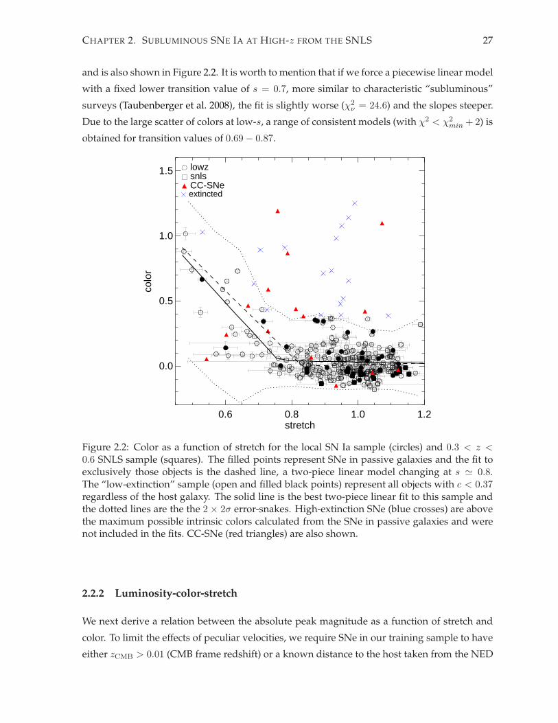
CHAPTER 2. SUBLUMINOUS SNE IA AT HIGH-z FROM THE SNLS 27
and is also shown in Figure 2.2. It is worth to mention that if we force a piecewise linear model
with a fixed lower transition value of s = 0.7, more similar to characteristic “subluminous”
surveys (Taubenberger et al. 2008), the fit is slightly worse (χ2ν = 24.6) and the slopes steeper.
Due to the large scatter of colors at low-s, a range of consistent models (with χ2 < χ2min + 2) is
obtained for transition values of 0.69 − 0.87.
0.6 0.8 1.0 1.2stretch
0.0
0.5
1.0
1.5
colo
r
lowzsnlsCC-SNeextincted
Figure 2.2: Color as a function of stretch for the local SN Ia sample (circles) and 0.3 < z <0.6 SNLS sample (squares). The filled points represent SNe in passive galaxies and the fit toexclusively those objects is the dashed line, a two-piece linear model changing at s ≃ 0.8.The “low-extinction” sample (open and filled black points) represent all objects with c < 0.37regardless of the host galaxy. The solid line is the best two-piece linear fit to this sample andthe dotted lines are the the 2 × 2σ error-snakes. High-extinction SNe (blue crosses) are abovethe maximum possible intrinsic colors calculated from the SNe in passive galaxies and werenot included in the fits. CC-SNe (red triangles) are also shown.
2.2.2 Luminosity-color-stretch
We next derive a relation between the absolute peak magnitude as a function of stretch and
color. To limit the effects of peculiar velocities, we require SNe in our training sample to have
either zCMB > 0.01 (CMB frame redshift) or a known distance to the host taken from the NED

CHAPTER 2. SUBLUMINOUS SNE IA AT HIGH-z FROM THE SNLS 28
database2.
We fit simultaneously magnitude, stretch and color to different models. The best one is
again bilinear in both, stretch and color. The absolute magnitude shows a steeper slope as a
function of color for redder objects changing at c ≃ 0.07 (upper panel, Figure 2.3). Against
stretch, the magnitude values (lower panel, Figure 2.3) are also well fit by a bilinear model
with a shallower slope for the low-s stretch range. The effects in the differing slopes are not as
strong as for the color-stretch relation but they will make the posterior analysis more precise.
The errors in the absolute magnitude (from the apparent magnitude and redshift errors) and
in the stretch and color are included in the fit. The magnitude-stretch-color relation can be
summarized as follows:
MB = M + α[1,2] (s − 1) + β[a,b] c + Mmatch[2,b] (2.2)
with M = −19.11 ± 0.01, and where α1 = −1.19 ± 0.03 and α2 = −0.54 ± 0.09 are respec-
tively used for stretch values greater and lower than the transition value of s = 0.82 ± 0.02.
βa = 3.00±0.02 and βb = 2.15±0.05 are used for values of c greater and lower than 0.07±0.01,
respectively. Mmatch2 = −0.18(α1−α2) and Mmatch
b = 0.07(βa−βb) unite the fit at the changing
values. This model results in a slightly better fit (χ2ν = 19.6) than other models (e. g. exponen-
tial –in stretch and color– with χ2ν = 19.9).
We include an asymmetric error-snake on these relations, shown by the dotted lines in
Figures 2.2 and 2.3. These delimit (twice) the region within which 95% of all SNe Ia in each
bin of 0.1 in color and 0.07 in stretch are found around the best model. The width of the
region has been doubled to allow for the larger photometric scatter of the high-z SNe, which
will be important later in §2.3.2. This region also covers any uncertainties in the relations
modeled in this section and allows for scatter in the color of the SNe. Requiring all objects
to be inside those error-snakes, i.e. color-stretch, magnitude-color and magnitude-stretch, we
find that ≃ 90% of the normal and low-s SNe Ia pass the cut (see Table 2.3). However, only
2 contaminants (all SNe Ib/c) survive the same cull, a ≃ 6% of the total of contaminants (or
“contamination rate”). We find this tradeoff to be beneficial. Reducing the contamination is
useful when limiting the systematic errors as discussed in §2.4.3.
2The distance to a galaxy provided by NED is a mean of different available distance measurements from theliterature such as Cepheids, RR Lyrae stars, Tully-Fisher, Surface Brightness Fluctuations, etc. It depends on thechosen Hubble constant modified by local flow parameters. The error corresponds to the standard deviation ofthese measurements.

CHAPTER 2. SUBLUMINOUS SNE IA AT HIGH-z FROM THE SNLS 29
-0.2 0.0 0.2 0.4 0.6 0.8 1.0 1.2color
-20
-19
-18
-17
-16
-15
MBs-
corr
s>0.8s<0.8CC-SNe
0.6 0.8 1.0 1.2stretch
-20
-19
-18
-17
-16
MBc-
corr
lowzsnlsCC-SNe
Figure 2.3: Absolute magnitude (corrected for stretch from Eq. 2.2, i. e. M s−corrB = MB −
α[1,2](s − 1) − Mmatch2 ) vs color (upper) and absolute magnitude (corrected for color, i. e.
M c−corrB = MB − β[a,b]c − Mmatch
b ) vs stretch (lower) for the training sample. The solid linesrepresent the best fit model, a two-piece linear model for each case. The dashed lines arerespectively the 2 × 2σ error-snakes. CC-SNe (red triangles) are also shown.

CHAPTER 2. SUBLUMINOUS SNE IA AT HIGH-z FROM THE SNLS 30
2.3 High-z low-stretch candidate selection
The search component of the SNLS, carried out using the Canada-France-Hawaii Telescope
(CFHT), is a wide field imaging survey well-suited to the detection of SNe Ia in the red-
shift range 0.1 ≤ z <∼ 1.0 (Astier et al. 2006). It is a rolling search where four 1 × 1 fields
(D1 to D4) are imaged every few days, so that a well sampled LC is obtained in four filters
(gMrM iMzM ) for each discovered supernova (see Perrett et al. 2010 for a review). Good can-
didates are followed-up spectroscopically. Because they are faint, less frequent, and not vital
for cosmological studies, typical subluminous SNe Ia are not prioritized in the spectroscopic
follow-up (Sullivan et al. 2006a; Perrett et al. 2010). We can still use the well-sampled SNLS
multi-wavelength LCs to photometrically identify these objects. The method used resembles
the one for the normal-stretch population of Perrett et al. (2011, hereafter P11), although with
appropriate adjustments for the low-s objects. This makes a direct comparison with the differ-
ent stretch populations possible.
During the first 4 years of operation, up to July 2007, the candidate database consists of
more than 5000 photometric transients including AGN, non-SNe and CC-SNe. As in P11,
candidates in masked areas of the deep stacks are removed, as well as objects that lack the
necessary LC coverage for a good photometric identification and parameterization. These
observational criteria reduce the sample to half and are the same ones used for the SNLS
training sample in §4.2: at least one gM observation between −15 and 5 days of maximum, at
least one rM and one iM observations between −15 and +2.5 days of maximum, at least one
rM and one iM observations between−9 and +7 days of maximum, and at least one rM or one
iM observation between +5 and +20 days of maximum.
2.3.1 Redshift estimation and LC fit
In P11, accurate photometric redshifts from the SNe were obtained with the use of two normal
SN Ia LC fitters. Their approach requires a good spectroscopic sample for testing the method
and the precision of the final photometric redshifts. We do not possess any 91bg-like SN Ia
spectrum at high redshift with clear Ti 2 features, only 3 low-s objects at the border of our
defintion, s<∼ 0.8, that have spectra of rather normal SNe Ia. The high degree of degeneracy
in the LC fits, particularly with stretch and redshift, which compete to make an object appear
faint, demand an unbiased redshift estimate that will lead to appropriate LC parameters like
stretch and color.
Several hundred objects of the 4-year dataset possess spectroscopic redshifts (spec-z) from
either the SN or from the host galaxy. For the SN-derived redshifts, the SN type has been
determined from the spectra in the majority of cases (Howell et al. 2005; Bronder et al. 2008;

CHAPTER 2. SUBLUMINOUS SNE IA AT HIGH-z FROM THE SNLS 31
Ellis et al. 2008; Balland et al. 2009; Walker et al. 2010). Most of these are normal SNe Ia (413),
although a good sample of CC objects is also available (78). The host spec-z include data
from DEEP/DEEP2 (Davis et al. 2003), VVDS (Le Fevre et al. 2005), zCOSMOS (Lilly et al.
2007) and VIMOS (Jonsson et al. 2011). Many candidates without spectroscopic redshifts have
host photometric redshifts from the SNLS broad-band photometry either using the spectral
connectivity analysis method of Freeman et al. (2009), or, when no match is found, through
fits to spectral energy distributions as in Sullivan et al. (2006b). The resulting host photo-z,
zhostphot, are very good to z ≃ 0.75 with |∆z|(1+zspec)
= 0.042 and a low (∼ 5%) catastrophic failure
rate (|zspec−zhostphot|
(1+zspec)> 0.15).
Fortunately, some of those SNe Ia with catastrophic redshifts can be identified with the
help of the two LC fitters of P11 adjusted for low-s SN: estimate sn (Sullivan et al. 2006a)
and the aforementioned modified version of SiFTO (see §4.2). Their use in the multi-step
process explained below provides good quality-of-fit parameters capable of distinguishing
SNe Ia from CC-SNe, but also offer an independent mechanism for obtaining photometric
redshifts using the SN, zSNphot, in cases where host redshifts are lacking.
Once the redshift is known, SiFTO is used to obtain the stretch and color of each SN. Tests
on the local sample (§4.2) show that it works well without imposing any stretch-color model.
As shown in Figure 2 of P11, the derived stretch is largely independent of the redshift be-
cause the rise and fall of SNe Ia are faster at shorter wavelengths, which largely compensates
for redshift uncertainties. In Figure 2.4, we demonstrate that this behavior extends to low-s
objects. Shifting the redshift –either photometric or spectroscopic– for each SN in our final
low-s sample (see §2.3.2) by as much as ∆z = ±0.3, we obtain a stretch variation lower than
∼ s± 0.1. While this shows more dependence on redshift than the normal-stretch population,
it still allows us to obtain accurate stretch estimates even in the presence of moderate redshift
uncertainties.
The estimate sn routine is described in more detail in Sullivan et al. (2006a). It performs
a grid search on the χ2 of a fit to SN photometry in flux space to a five-parameter model,
including redshift. For this analysis, we modified it to include low-s objects using the color-
stretch relations of Eq. 2.1, and the magnitude relation of Eq. 2.2. This fit depends on the
assumed values of the cosmological parameters.
We calculated the SN photo-z for all objects in a similar fashion to P11 using the following
multi-step process: First, we use estimate sn to get a preliminary redshift estimate. We then
use this redshift as a fixed input to a SiFTO fit to obtain an improved stretch measurement.
Finally, we feed back this stretch to a final estimate sn fit as a fixed parameter to obtain a
more accurate zSNphot. We use this SN photo-z for SNe that do not have any other redshift
(spectroscopic or host photometric).

CHAPTER 2. SUBLUMINOUS SNE IA AT HIGH-z FROM THE SNLS 32
-0.3 -0.2 -0.1 0.0 0.1 0.2 0.3∆ z
-0.2
-0.1
0.0
0.1
0.2
∆ s
photo low-s Iaspec low-s Ia
0.50 0.55 0.60 0.65 0.70 0.75 0.80s at best z
0.5
0.6
0.7
0.8
0.9
Mea
n s
photo low-s Iaspec low-s Ia
Figure 2.4: Upper: The change in fit stretch due to the deliberate variation in redshift for thelow-s final sample of §2.3.2. The blue squares represent the spectroscopically-confirmed low-sSNe Ia. The solid black lines are the standard deviation above the median ∆s. Lower: Theaverage output stretch for each SN Ia as a function of its stretch (at zero redshift offset). Theerror bars are the change due to the variation in redshift for each SN Ia.

CHAPTER 2. SUBLUMINOUS SNE IA AT HIGH-z FROM THE SNLS 33
Objects with zhostphot that have “bad fits”, i.e. that do not pass all cuts of §2.3.2, are not
discarded, but instead the cuts are re-applied using zSNphot. If this also fails, then the object is
rejected. This offers some protection against catastrophic host photo-z failures. This recovers
29 confirmed SNe Ia. All known contaminants fail with both photo-z values, so we are con-
fident that this procedure still rejects non-Ias. This process is summarized in a flow diagram
(Figure 2.5).
SiFTO(free s)
HOST PHOTO−Zpassed cuts
of $2.3.2
passed cutsof $2.3.2
ESTIMATE_SN(free z, free s)
SiFTO(free s)
z input s input ESTIMATE_SN(free z)
SiFTO(free s)
z input
NOT SNIa
of $2.3.2did not pass cuts
did not pass cutsof $2.3.2
SNIa with z,s,c
Figure 2.5: Flow diagram showing how SN Ia candidates without spectroscopic redshift areselected and how their photometric redshift is measured. If the objects do not have a photo-metric redshift estimate from the host or they fail to pass the selection cuts with that redshift,then the two LC fitters, estimate sn and SiFTO are used to estimate a SN photo-z.
2.3.2 Final candidates
We perform final SiFTO (and low-s-modified estimate sn) fits to each object to obtain the
parameters of each SN and quality-of-fit values. A series of cuts are then applied to screen out
objects with poorly estimated parameters or those unlikely to be SNe Ia. A summary of the
applied culls and the number of objects surviving each of them can be found in Table 2.4. The
χ2 culls are similar to those of P11, although we weaken the requirements slightly for s ≤ 0.8
objects based on the study of the low-z sample: reduced χ2s of χ2estimate sn < 13 for the overall
fit, and for individual passbands χ2estimate sn(rM ) < 11 and χ2
estimate sn(iM ) < 16, and a SiFTO
cull of χ2SiFTO < 11. Additionally, we require the objects to be inside the error-snakes trained
in §4.2 with low-z low-s SNe in order to constrain their parameters (Figure 2.7). These cut
values are derived empirically by trying to minimize the number of known contaminants that
pass and minimize the number of rejected confirmed SNe Ia.

CHAPTER 2. SUBLUMINOUS SNE IA AT HIGH-z FROM THE SNLS 34
0.0 0.2 0.4 0.6 0.8 1.0 1.2zspec
0.0
0.2
0.4
0.6
0.8
1.0
1.2
z pho
t
specz-Iaspecz
low-s
Figure 2.6: Photometric redshifts obtained from the host or from the LC fits compared to spec-troscopic redshifts from the SN (open circles) or the host (filled circles). Purple stars represents ≤ 0.8 objects. The solid line shows 1:1 agreement and dashed lines a 10% uncertainty in(1 + zspec). The photo-z errors are either from the host or from estimate sn.
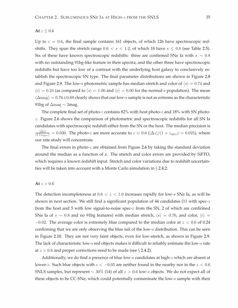
CHAPTER 2. SUBLUMINOUS SNE IA AT HIGH-z FROM THE SNLS 35
At z ≤ 0.6
Up to z = 0.6, the final sample contains 161 objects, of which 126 have spectroscopic red-
shifts. They span the stretch range 0.6 < s < 1.2, of which 18 have s ≤ 0.8 (see Table 2.5).
Six of these have known spectroscopic redshifts: three are confirmed SNe Ia with s ∼ 0.8
with no outstanding 91bg-like feature in their spectra, and the other three have spectroscopic
redshifts but have too low of a contrast with the underlying host galaxy to conclusively es-
tablish the spectroscopic SN type. The final parameter distributions are shown in Figure 2.8
and Figure 2.9. The low-s photometric sample has median stretch and color of 〈s〉 = 0.74 and
〈c〉 = 0.24 (as compared to 〈s〉 = 1.00 and 〈c〉 = 0.00 for the normal-s population). The mean
〈∆mag〉 = 0.76±0.69 clearly shows that our low-s sample is not as extreme as the characteristic
91bg of ∆mag ∼ 2mag.
The complete final set of photo-z contains 82% with host photo-z and 18% with SN photo-
z. Figure 2.6 shows the comparison of photometric and spectroscopic redshifts for all SN Ia
candidates with spectroscopic redshift either from the SN or the host. The median precision is|∆z|
(1+zspec)= 0.030. The photo-z are more accurate to z ≃ 0.6 (|∆z|/(1 + zspec) = 0.025), where
our rate study will concentrate.
The final errors in photo-z are obtained from Figure 2.6 by taking the standard deviation
around the median as a function of z. The stretch and color errors are provided by SiFTO,
which requires a known redshift input. Stretch and color variations due to redshift uncertain-
ties will be taken into account with a Monte Carlo simulation in § 2.4.2.
At z > 0.6
The detection incompleteness at 0.6 < z < 1.0 increases rapidly for low-s SNe Ia, as will be
shown in next section. We still find a significant population of 44 candidates (11 with spec-z
from the host and 5 with low signal-to-noise spec-z from the SN, 2 of which are confirmed
SNe Ia of s ∼ 0.8 and no 91bg features) with median stretch, 〈s〉 = 0.76, and color, 〈c〉 =
−0.02. The average color is extremely blue compared to the median color at z < 0.6 of 0.24
confirming that we are only observing the blue tail of the low-s distribution. This can be seen
in Figure 2.10. They are not very faint objects, even for low-stretch, as shown in Figure 2.9.
The lack of characteristic low-s red objects makes it difficult to reliably estimate the low-s rate
at z > 0.6 and proper corrections need to be made (see § 2.4.2).
Additionally, we do find a presence of blue low-s candidates at high-z which are absent at
lower-z. Such blue objects with c < −0.05 are neither found in the nearby nor in the z < 0.6
SNLS samples, but represent ∼ 30% (14) of all z > 0.6 low-s objects. We do not expect all of
these objects to be CC-SNe, which could potentially contaminate the low-s sample with their

CHAPTER 2. SUBLUMINOUS SNE IA AT HIGH-z FROM THE SNLS 36
0.6 0.8 1.0 1.2stretch
-0.5
0.0
0.5
1.0
1.5
colo
r
AllIaNon-Ia
-0.2 0.0 0.2 0.4 0.6 0.8 1.0 1.2color
-20
-19
-18
-17
-16
-15
MBco
rr
AllIaNon-Ia
0.5 0.6 0.7 0.8 0.9 1.0 1.1 1.2stretch
-20
-19
-18
-17
-16
MBco
rr
AllIaNon-Ia
Figure 2.7: Color-stretch (left), magnitude-color (middle) and magnitude-stretch (right) for allSNLS objects passing the observation criteria (open points) and the final SN Ia photometricz < 0.6 sample after all cuts of Table 2.4 (filled points). Spectroscopically-confirmed SNe Ia(blue squares) and non-Ia (red triangles) are shown. The lines are the best-fit relations anderror-snakes found in §4.2 for the local training sample, and served as additional cuts.

CHAPTER 2. SUBLUMINOUS SNE IA AT HIGH-z FROM THE SNLS 37
0.1 0.2 0.3 0.4 0.5 0.6redshift
0
20
40
60
80
N
Photo-IaSpec-Ialow-s
0.6 0.7 0.8 0.9 1.0 1.1 1.2stretch
0
10
20
30
40
N
Photo-IaSpec-Ia
0.0 0.2 0.4 0.6 0.8color
0
10
20
30
40
N
Photo-IaSpec-Ialow-s
Figure 2.8: Final distributions in redshift (left), stretch (center) and color (right) of the z < 0.6SN Ia photometric sample including low-s. The white histogram is the whole population, thegray is the spectroscopically-confirmed SNe Ia and the black the low-s candidates.
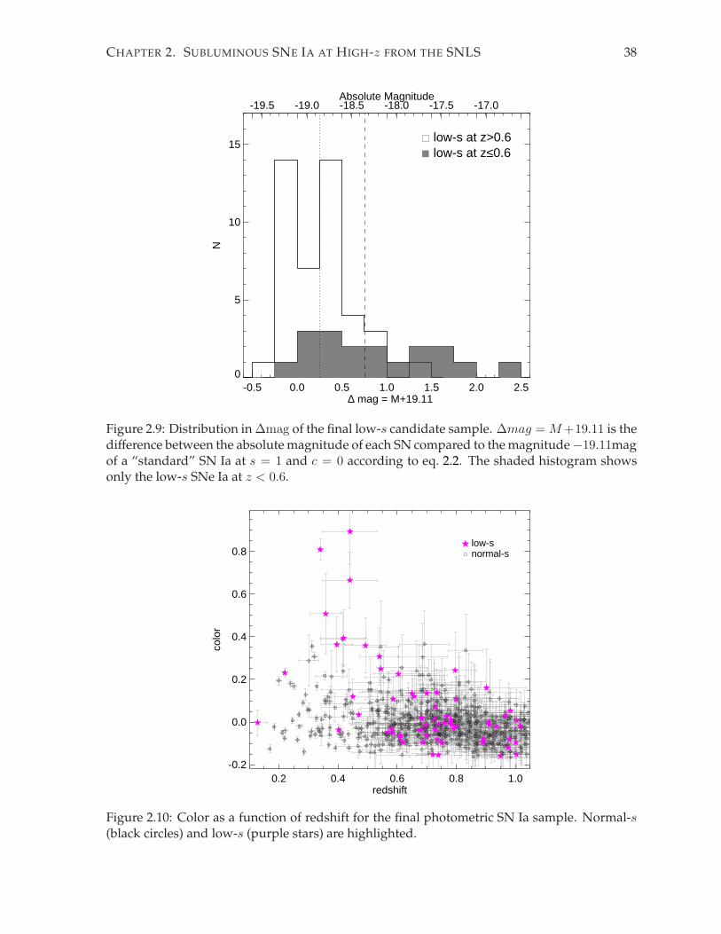
CHAPTER 2. SUBLUMINOUS SNE IA AT HIGH-z FROM THE SNLS 38
-0.5 0.0 0.5 1.0 1.5 2.0 2.5∆ mag = M+19.11
0
5
10
15
N
-19.5 -19.0 -18.5 -18.0 -17.5 -17.0Absolute Magnitude
low-s at z>0.6low-s at z≤0.6
Figure 2.9: Distribution in ∆mag of the final low-s candidate sample. ∆mag = M +19.11 is thedifference between the absolutemagnitude of each SN compared to themagnitude−19.11magof a “standard” SN Ia at s = 1 and c = 0 according to eq. 2.2. The shaded histogram showsonly the low-s SNe Ia at z < 0.6.
0.2 0.4 0.6 0.8 1.0redshift
-0.2
0.0
0.2
0.4
0.6
0.8
colo
r
normal-slow-s
Figure 2.10: Color as a function of redshift for the final photometric SN Ia sample. Normal-s(black circles) and low-s (purple stars) are highlighted.

CHAPTER 2. SUBLUMINOUS SNE IA AT HIGH-z FROM THE SNLS 39
characteristic bluer colors. As will be shown later, besides going through our SN Ia pipeline,
the environment of these candidates is not characteristic of CC-SNe.
A second possibility is that this group represents another class of transients that are fast and
blue. The object found by Perets et al. (2010) is faint and fast-evolving but with clear different
spectroscopic features and bluer colors than 91bg-like objects. It is hosted in an old stellar
population as well as most of our candidates. However, our objects are not as faint (Figure 2.9).
On the other hand, the transients found by Poznanski et al. (2010) and Kasliwal et al. (2010),
suggested SN .Ia-like helium detonations of a WD, are blue and of similar brightness than
ours, but evolve faster. When fit with our templates, we obtain very poor fits with s = 0.44
and s = 0.33, respectively, lower than our lower stretch limit for subluminous SNe Ia.
A tempting explanation is that the input photometric redshift for the LC fit is consistently
wrong and affects the obtained color and stretch. This hypothesis is ruled out because 7 of
these objects have spectroscopic redshift and the rest (except one) have photometric redshift
from the host (with mean photo-z error of ∼ 0.08), which do not show any significant sys-
tematic. We have seen the small effect in the measured stretch when the redshift is varied
(Figure 2.4). We now show the effect in the magnitude and color of photometric candidates in
Figure 2.11. Their variation due to changes in photo-z cannot account for all the bluer colors
but for some of them –only if the redshifts were all consistently overestimated by +0.05, the
colors would be redder by +0.08 (and magnitudes fainter by +0.17, whereas stretches would
only change by −0.004).
Photometric errors in stretch and color get larger as we probe higher redshifts. Most of the
candidates found at these redshifts have stretch close to the limiting definition of s = 0.8, so
that they are consistentwith being fast normal-s SNe Ia. Only 3 candidates have s+serror < 0.8,
one of them with s < 0.6. Of these,two also have c + cerror < −0.05, inconsistent with typical
low-s colors, and will be further discussed in 2.4.3. The rest can therefore be explained as
the blue tail of s ∼ 0.8 objects while the redder counterpart remains unseen due to selection
effects. In the remainder of this work, we treat this group as such and correct for this selection
bias when calculating the rates.
2.4 Low-stretch SN Ia rate evolution
With a set of low-s candidates, we proceed to calculate a volumetric rate as a function of
redshift. As in P11, the volumetric rate, rb(zb), for a given redshift bin, represented here by the
middle of the redshift bin, zb, is given by the sum over all Nb candidates inside the bin:

CHAPTER 2. SUBLUMINOUS SNE IA AT HIGH-z FROM THE SNLS 40
-0.2 0.0 0.2 0.4 0.6color
-19.5
-19.0
-18.5
-18.0
-17.5
Abs
olut
e m
agni
tude
low-s at z≤0.6low-s at z>0.6
Figure 2.11: Absolute magnitude vs color for the low-s SN Ia sample with photo-z at z < 0.6(big open pink stars) and at z > 0.6 (small filled purple stars). The dots show the normal-s sample. The upward and downward arrows show the new magnitudes and colors whenvarying the photo-z by +0.05 and −0.05 respectively. The lines unite the same object at thethree redshifts. The lower right error bars represent the typical (mean) photometric errors.
rb(zb) =1
Vb
Nb∑
i=1
(1 + zi)
ǫi∆Ti, (2.3)
where ǫ is the individual SN detection efficiency depending on the characteristics of each
object (like redshift, stretch and color) and∆T is the sampling time accessible to find the object,
divided by (1 + z) to account for time dilation. Vb is the comoving volume contained in the
redshift range of the bin.
2.4.1 Detection efficiencies
The detection efficiencies ǫi account for observing biases measuring the rate. They depend
on numerous factors and are specified as a function of the SN characteristics such as redshift,
stretch and color (along with field and year of observation). The efficiencies used here are
described in P11 and Perrett et al. (2010), and are based on a Monte-Carlo study of 2.4 million
artificial SNe Ia injected into the actual SNLS images. This approach avoids the need to make
assumptions about temporal and spatial data coverage.
The artificial SNe are generated using uniform distributions of redshift and stretch (down
to s = 0.5), and the color is determined using a relation like Eq. 2.1, including an intrinsic scat-

CHAPTER 2. SUBLUMINOUS SNE IA AT HIGH-z FROM THE SNLS 41
ter around the stretch-color relation (a Gaussian noise with dispersion σ = 0.04 added inde-
pendently to U and V ). The peak magnitudes are generated from the luminosity-stretch-color
relation, as in Eq. 2.2, and the redshift and assumed cosmology, plus an additional unmodeled
magnitude dispersion from a Gaussian distribution with an intrinsic scatter of σint = 0.15.
The LC is generated from integrating, at a given epoch and through the filter functions, the
SN Ia spectral templates scaled for the B-magnitude and corrected for U − B and B − V
colors, Milky Way and host extinction. The artificial SN is then inserted into each iM image
obtained by the SNLS. The images are then processed through the same pipeline used in the
real-time SN discovery, and the recovered fraction is used to derive the efficiency as a function
of various parameters, including redshift, stretch, color, observing season and field (see amore
detailed description in Perrett et al. 2010). The low-s candidates, which are faint, red and have
a rapid rise and fall, are more difficult to detect and therefore have a lower efficiency, so are
accordingly given a higher weight when calculating the rates.
The efficiencies are calculated in bins of width ∆z = ∆s = ∆c = 0.1. The measured effi-
ciencies, linearly interpolated according to each SN, are shown in Figure 2.12. It can be seen
that the mean efficiencies are lower for the low-s sample up to z ∼ 0.6. Above z = 0.6, the
mean efficiencies seem to approach the normal-s sample. At these redshifts they become low
for all but the bluest low-s objects. This leads to a higher fraction of low-s blue objects with
very few red ones recovered, as found in § 2.3.2. We show the expected efficiency distribu-
tion for the missing red, low-s SNe Ia of an unevolving color distribution as green squares
in Figure 2.12 based on the observed low-s color distribution at low redshift from §2.8. The
rates at z > 0.6 will need to be corrected for these missing objects (see next section). We note
that the efficiencies shown in Figure 2.12 are the raw efficiencies –the recovery fraction from
the simulated SNe– without the observational constraints of section § 2.3 nor the sampling
time correction that depends on each field and season. These corrections can make the actual
efficiencies much lower (see P11). For instance, one of our low-s candidates at high-z with
z = 0.80, s = 0.63 and c = 0.24 has a raw efficiency of 0.54 but with observational constraints
and sampling time this efficiency is only 0.18, which explains why these objects are hard to
observe.
2.4.2 SN Ia Rates and Monte-Carlo simulations
We calculate a rate evolution, rmeas, shown in Column 5 of Table 2.6 solely based on Eq. 2.3
and with the efficiencies from § 2.4.1. We use bins of ∆z = 0.2 due to the low sample statistics
(the last z-bin is only 0.1 wide as no low-s candidate exists beyond z = 1). The measured
errors in stretch and color from the LC fit, and especially the errors in the photometric redshift
of each candidate, can lead to uncertainties in the rate measurement. We account for these

CHAPTER 2. SUBLUMINOUS SNE IA AT HIGH-z FROM THE SNLS 42
0.2 0.4 0.6 0.8 1.0redshift
0.2
0.4
0.6
0.8
1.0
effic
ienc
y
normal-slow-ssim low-s
Figure 2.12: Efficiencies calculated by P11 for the SN Ia photometric sample for normal-s(black circles) and low-s (purple stars) populations. For objects where no direct efficiencywas found (small filled stars), the closest match in color was used. Mean values in redshiftbins for normal-s and low-s populations (big filled circles and stars) are shown. Additionally,simulated low-s objects for z > 0.6 bins (green squares) based on the z < 0.6 color distributionand respective mean (green dashed line) are shown for comparison. Note that these efficien-cies do not include the observation criteria of section § 2.3 and sampling time correction of thedifferent fields observed.
via a Monte-Carlo (MC) simulation that randomly shifts the photometric redshift according to
its error (for those SNe Ia with photo-z). For each redshift, a corresponding LC fit provides
new parameters and its covariance matrix. This latter is used to generate a new random set of
stretch and color using standard techniques (James & Roos 1975). We recalculate the rates from
Eq. 2.3 for each iteration based on the randomized values, and use the median value over the
1000 realizations to determine the final rate, rMC. We estimate the error from the variance of the
rates in each bin (and call them “MC” errors shown in Column 6 of Table 2.6 and Figure 2.13)
and add it in quadrature to the weighted 1σ Poisson statistical errors in Figure 2.13 (confidence
levels calculated using the Clopper-Pearson method used for example in Gehrels 1986). The
error simulation differs from P11, as the SNLS does not possess a known spectroscopic sample
of low-s SNe Ia from which we could obtain parameter distributions. Instead, we treat each
SN individually by randomly drawing parameters according to its errors and covariances.
Although the precise details of our simulation differ from P11, a SN Ia rate evolution within
the errors is obtained. It is worthwile to mention that this MC approach handles interlopers
from the s > 0.8 population leaking into the low-s sample (and vice-versa) by taking into
account the stretch uncertainties in the simulation.
Additionally, we have seen in the previous section that we do not find red objects in the

CHAPTER 2. SUBLUMINOUS SNE IA AT HIGH-z FROM THE SNLS 43
10-6
10-5
10-4
SN
Ia R
ate
(eve
nts
yr-1M
pc-3h3 70
)
0.0 0.2 0.4 0.6 0.8 1.0Redshift
13 9 7 6Age of the universe (billions of years)
s≤ 0.8s>0.8All
s≤0.8 corr
Figure 2.13: Volumetric rate of low-s SNe Ia as a function of redshift (green open points)compared to the normal-s rate (blue squared points) of P11. The total summed rate (bluefilled points) is shown with a little z-offset for clarity. The stars represent the corrected high-z low-s rate calculated from real and simulated objects drawn from a distribution scaled tothe z < 0.6 color distribution. The filled triangle is the total nearby SN Ia rate from Li et al.(2010b) and the open triangle is the low-s rate estimated from a s ≤ 0.8 fraction of it. Thesolid lines are the best A + B model and uncertainties found in P11. The dashed lines are thebest A-model and uncertainties found in this study through a fit of only SNLS z < 0.6 bins:A = (1.05 ± 0.28) × 10−14 SNeyr−1M−1
⊙ .

CHAPTER 2. SUBLUMINOUS SNE IA AT HIGH-z FROM THE SNLS 44
higher-z bins. This selection bias results in underestimated rate values at high-z, which are
not corrected in the MC by the efficiencies of the bluer objects found. There is a lack of objects
in certain red color bins, so that no efficiency can account for them. To measure this effect, we
take the low-s distribution of color in an underestimated high-z bin (for eachMC iteration), we
normalize this distribution to the known color distribution at z < 0.6 (right Figure 2.8), which
has already been corrected for the efficiencies of each SN, and then generate fake SNe in the
missing color bins. The normalization is done with the two bluest matching bins. Figure 2.14
shows an example for 0.7 < z < 0.9. The green open histogram is the final corrected histogram
from the initial observed diagonal-shaded distribution. The correcting factor for this case is
fb,corr = 1 + Nb(fake)Nb
= 1.9, where Nb(fake) is the number of generated SNe in the bin and Nb
is the observed number, so that the corrected rate is rb,corr = rb × fb,corr. The final correcting
factors from the median of all MC iterations, summed Poisson (from the number of objects
used in the bins used to normalize both distributions) and MC errors, as well as the resulting
corrected rates are shown in the last two columns of Table 2.6. In Figure 2.13, the corrected
rates are shown as stars.
-0.2 0.0 0.2 0.4 0.6 0.8color
0
2
4
6
8
10
12
N
z ≤ 0.6
0.70<z≤0.90
0.70<z≤0.90 CORR
factor:1.88
Figure 2.14: Example of how the observed color distribution (of one MC iteration) for low-sat 0.7 < z < 0.9 (diagonal-shaded) is corrected to match the efficiency-corrected low-s colordistribution at z < 0.6 (shaded). The final corrected color distribution for that z-bin (openhistogram) has fb = 1.88 more SNe than the original observed one.
Finally, errors in the efficiencies can affect the rate values. As explained in P11, those
CHAPTER 2. SUBLUMINOUS SNE IA AT HIGH-z FROM THE SNLS 45
come mainly from systematic errors in the underlying assumed ∆mag distribution of SNe Ia,
the distribution of residuals between the absolute magnitude of a fiducial s = 1 SN Ia and
the magnitudes of observed SNe Ia after correction for stretch and color. To check for this
systematic error, we allow for random efficiencies in the MC simulation calculated from a
range of σint = 0.12 − 0.15 in the ∆mag distribution, obtaining results that agree very well
with the rates of Figure 2.13.
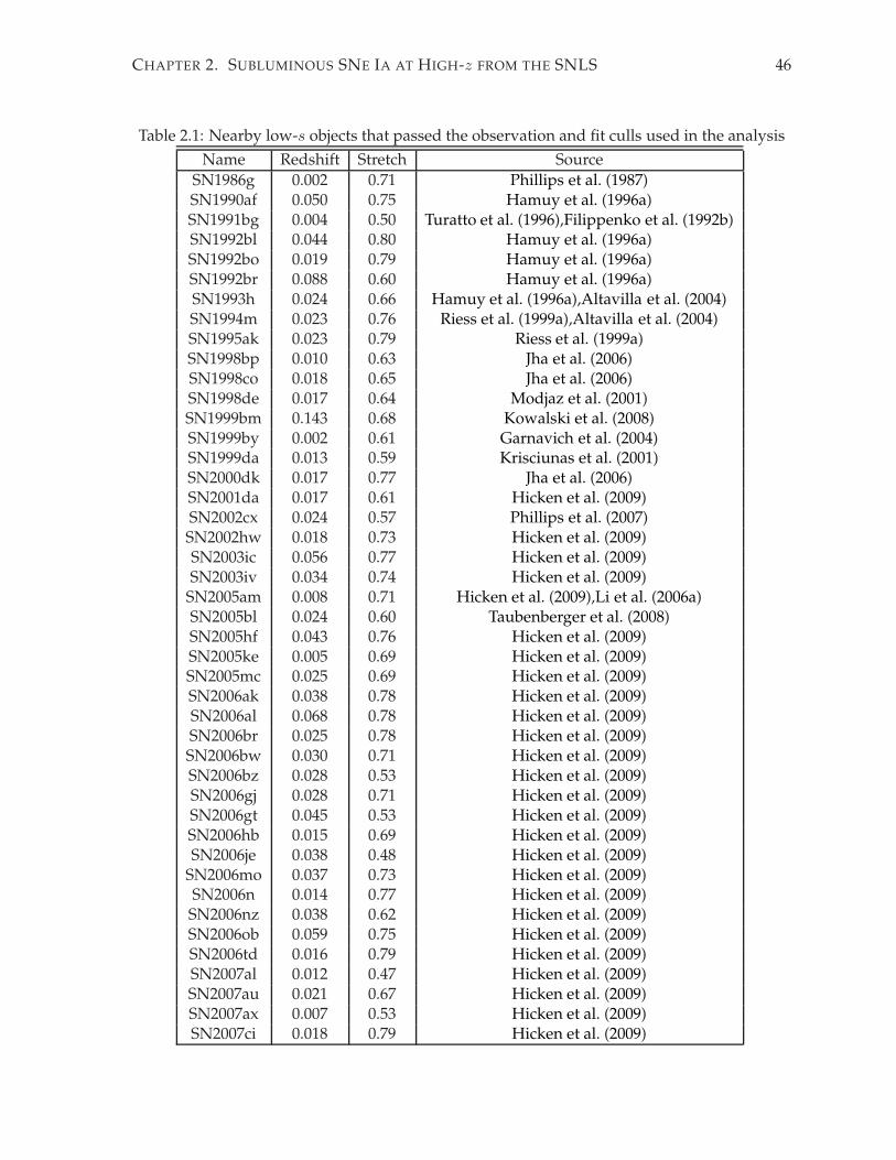
CHAPTER 2. SUBLUMINOUS SNE IA AT HIGH-z FROM THE SNLS 46
Table 2.1: Nearby low-s objects that passed the observation and fit culls used in the analysis
Name Redshift Stretch Source
SN1986g 0.002 0.71 Phillips et al. (1987)SN1990af 0.050 0.75 Hamuy et al. (1996a)SN1991bg 0.004 0.50 Turatto et al. (1996),Filippenko et al. (1992b)SN1992bl 0.044 0.80 Hamuy et al. (1996a)SN1992bo 0.019 0.79 Hamuy et al. (1996a)SN1992br 0.088 0.60 Hamuy et al. (1996a)SN1993h 0.024 0.66 Hamuy et al. (1996a),Altavilla et al. (2004)SN1994m 0.023 0.76 Riess et al. (1999a),Altavilla et al. (2004)SN1995ak 0.023 0.79 Riess et al. (1999a)SN1998bp 0.010 0.63 Jha et al. (2006)SN1998co 0.018 0.65 Jha et al. (2006)SN1998de 0.017 0.64 Modjaz et al. (2001)SN1999bm 0.143 0.68 Kowalski et al. (2008)SN1999by 0.002 0.61 Garnavich et al. (2004)SN1999da 0.013 0.59 Krisciunas et al. (2001)SN2000dk 0.017 0.77 Jha et al. (2006)SN2001da 0.017 0.61 Hicken et al. (2009)SN2002cx 0.024 0.57 Phillips et al. (2007)SN2002hw 0.018 0.73 Hicken et al. (2009)SN2003ic 0.056 0.77 Hicken et al. (2009)SN2003iv 0.034 0.74 Hicken et al. (2009)SN2005am 0.008 0.71 Hicken et al. (2009),Li et al. (2006a)SN2005bl 0.024 0.60 Taubenberger et al. (2008)SN2005hf 0.043 0.76 Hicken et al. (2009)SN2005ke 0.005 0.69 Hicken et al. (2009)SN2005mc 0.025 0.69 Hicken et al. (2009)SN2006ak 0.038 0.78 Hicken et al. (2009)SN2006al 0.068 0.78 Hicken et al. (2009)SN2006br 0.025 0.78 Hicken et al. (2009)SN2006bw 0.030 0.71 Hicken et al. (2009)SN2006bz 0.028 0.53 Hicken et al. (2009)SN2006gj 0.028 0.71 Hicken et al. (2009)SN2006gt 0.045 0.53 Hicken et al. (2009)SN2006hb 0.015 0.69 Hicken et al. (2009)SN2006je 0.038 0.48 Hicken et al. (2009)SN2006mo 0.037 0.73 Hicken et al. (2009)SN2006n 0.014 0.77 Hicken et al. (2009)SN2006nz 0.038 0.62 Hicken et al. (2009)SN2006ob 0.059 0.75 Hicken et al. (2009)SN2006td 0.016 0.79 Hicken et al. (2009)SN2007al 0.012 0.47 Hicken et al. (2009)SN2007au 0.021 0.67 Hicken et al. (2009)SN2007ax 0.007 0.53 Hicken et al. (2009)SN2007ci 0.018 0.79 Hicken et al. (2009)

CHAPTER 2. SUBLUMINOUS SNE IA AT HIGH-z FROM THE SNLS 47
Table 2.2: Nearby non-Ia SNe with acceptable SN Ia SiFTO fits, enough data coverage andfitted s ≤ 0.8.
Name Type Redshift Stretch Source
SN1999eu SNIIP 0.004 0.45 Pastorello et al. (2004)SN2001b SNIb 0.005 0.60 Tsvetkov (2006a)SN2002ao SNIbn 0.005 0.54 Pastorello et al. (2008b)SN2002ap SNIc 0.002 0.68 Gal-Yam et al. (2002b); Foley et al. (2003); Yoshii et al. (2003)SN2003jd SNIc 0.019 0.73 Valenti et al. (2008)SN2006aj SNIc 0.033 0.73 Pian et al. (2006); Sollerman et al. (2006)
Table 2.3: Culls applied to the training sample
Cull Number
confirmed confirmedSNe Ia(low-s) CC-SNe(low-s)low-z SNLS low-z SNLS
None 246(57) 112(3) 37(12) 47(9)observation 207(44) 106(3) 14(6) 21(4)
χ2SiFTO and snakes 184(41) 97(3) 2(2) 1(0)
Table 2.4: Culls applied to the SNLS sample
Cull Numberall low-s confirmed confirmed
SNe Ia CC-SNe
None 5234 1497 407 86observation 2615 837 343 62
χ2SiFTO 1054 144 338 22
χ2estimate sn 925 118 329 8
χ2f,estimate sn 848 109 303 5
snakes 710 70 295 1
FINAL 710 70 295 1z < 0.6 174 18 118 0

CHAPTER 2. SUBLUMINOUS SNE IA AT HIGH-z FROM THE SNLS 48
Table 2.5: SNLS low-s candidates at z ≤ 0.6
Name Redshift Source Redshift Stretch Colour
06D1ji zhostphot 0.36 ± 0.05 0.66 ± 0.05 0.51 ± 0.1904D2bt zSNspec 0.22 ± 0.00 0.79 ± 0.04 0.24 ± 0.0204D3df zSNspec 0.47 ± 0.01 0.78 ± 0.02 0.05 ± 0.0205D3jt zhostphot 0.49 ± 0.07 0.74 ± 0.05 0.36 ± 0.1306D3dh zhostphot 0.44 ± 0.09 0.66 ± 0.19 0.89 ± 0.1506D3ft zhostphot 0.42 ± 0.08 0.73 ± 0.04 0.39 ± 0.1305D3dw zhostphot 0.45 ± 0.09 0.73 ± 0.03 0.12 ± 0.0806D3dj zhostphot 0.44 ± 0.09 0.68 ± 0.12 0.67 ± 0.1303D4gi zhostspec 0.58 ± 0.00 0.76 ± 0.04 0.12 ± 0.0806D4gt zhostphot 0.59 ± 0.10 0.71 ± 0.03 −0.05 ± 0.0705D4ff zSNspec 0.40 ± 0.00 0.76 ± 0.02 −0.02 ± 0.0204D4ms zhostspec 0.57 ± 0.00 0.63 ± 0.08 0.02 ± 0.0603D4ah zhostphot 0.40 ± 0.05 0.74 ± 0.05 0.36 ± 0.1304D1po zhostphot 0.54 ± 0.07 0.69 ± 0.04 0.31 ± 0.1404D4hx zSNspec 0.55 ± 0.01 0.74 ± 0.03 0.26 ± 0.0605D3cn zhostphot 0.13 ± 0.03 0.80 ± 0.02 −0.00 ± 0.0606D1ce zSNphot 0.58 ± 0.10 0.79 ± 0.02 −0.03 ± 0.0607D3ek zSNphot 0.57 ± 0.10 0.78 ± 0.02 −0.05 ± 0.06
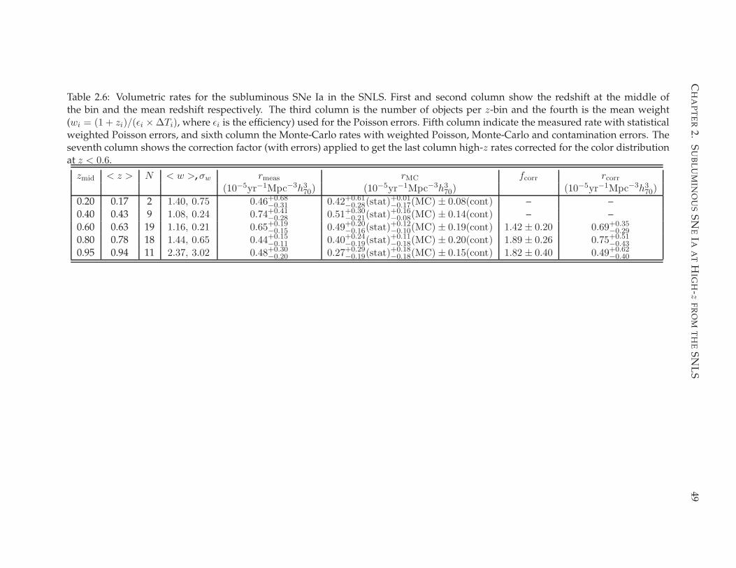
CHAPTER2.SUBLUM
INOUSSN
EIA
ATH
IGH-z
FROM
THESNLS
49
Table 2.6: Volumetric rates for the subluminous SNe Ia in the SNLS. First and second column show the redshift at the middle ofthe bin and the mean redshift respectively. The third column is the number of objects per z-bin and the fourth is the mean weight(wi = (1 + zi)/(ǫi × ∆Ti), where ǫi is the efficiency) used for the Poisson errors. Fifth column indicate the measured rate with statisticalweighted Poisson errors, and sixth column the Monte-Carlo rates with weighted Poisson, Monte-Carlo and contamination errors. Theseventh column shows the correction factor (with errors) applied to get the last column high-z rates corrected for the color distributionat z < 0.6.
zmid < z > N < w >, σw rmeas rMC fcorr rcorr
(10−5yr−1Mpc−3h370) (10−5yr−1Mpc−3h3
70) (10−5yr−1Mpc−3h370)
0.20 0.17 2 1.40, 0.75 0.46+0.68−0.31 0.42+0.61
−0.28(stat)+0.01−0.17(MC) ± 0.08(cont) – –
0.40 0.43 9 1.08, 0.24 0.74+0.41−0.28 0.51+0.30
−0.21(stat)+0.16−0.08(MC) ± 0.14(cont) – –
0.60 0.63 19 1.16, 0.21 0.65+0.19−0.15 0.49+0.20
−0.16(stat)+0.12−0.10(MC) ± 0.19(cont) 1.42 ± 0.20 0.69+0.35
−0.29
0.80 0.78 18 1.44, 0.65 0.44+0.15−0.11 0.40+0.24
−0.19(stat)+0.11−0.18(MC) ± 0.20(cont) 1.89 ± 0.26 0.75+0.51
−0.43
0.95 0.94 11 2.37, 3.02 0.48+0.30−0.20 0.27+0.29
−0.19(stat)+0.18−0.18(MC) ± 0.15(cont) 1.82 ± 0.40 0.49+0.62
−0.40

CHAPTER 2. SUBLUMINOUS SNE IA AT HIGH-z FROM THE SNLS 50
2.4.3 Contamination uncertainties
An important systematic error comes from core-collapse SNe mimicking the LC of low-s
SNe Ia. In P11, a missclassification fraction of less than ≤ 3% was found for the normal-s
population. We expect this fraction to be higher for low-s SNe Ia due to two effects. First,
they are dimmer, and more easily confused with the intrinsically fainter CC-SNe at a given
redshift. Second, as we probe higher redshift ranges, CC-SNe at low-z might masquerade as
low-s SNe Ia at higher-z since we do not have spectroscopic redshifts for all candidates. SNe II
have characteristic LCs that are very different from SNe Ia and present less danger of contami-
nation. SNe Ib/c, on the other hand, represent a smaller fraction of CC-SNe, ∼ 30% according
to Cappellaro et al. (1999); Smartt et al. (2009) and 25% according to Li et al. (2010a), but are
more similar to SNe Ia and will be the most probable contaminants.
The first error –where the photo-z is correct, yet the fit of a SN Ia template manages to pass
the quality-of-fit cuts– can be examined using the training sample (as in §4.2). We found a 6%
CC-SN missclassification rate, all SNe Ib/c. This fraction can be propagated to higher redshift
using the SN Ia rate evolution of P11, RIa(z) ∝ (1 + z)αIa with αIa ≃ 1.91, and a CC-SN rate
evolution reflecting the star formation rate from Hopkins & Beacom (2006), RCC ∝ (1 + z)αCC
with αCC ≃ 3.6. We assume a ratio of SNe Ia to CC-SNe of ∼ 0.22 at z = 0.3 from Bazin et al.
(2009), which translates to a local ratio of ∼ 0.39 – as compared to ∼ 0.48 found by Cappellaro
et al. (1999) and 0.24 from Li et al. (2010a) –. The percentage fraction of contamination as a
function of z, fcont(z), can then be described as:
fcont(z) =Npasscont(z)
Npass(z)=
1
1 + 0.39 r (1 + z)αIa−αCC, (2.4)
where r = 0.88/0.06 is the cull passing efficiency (the probability of a SN passing all selec-
tion criteria) ratio of Ia with respect to CC, assuming it does not evolve with z. This equation
allows us to get a crude estimate of the number of contaminants that would pass all cuts,
Npasscont(z). By dividing the expected fraction of contaminants per z-bin by the mean weight
of low-s SNe found therein (per MC simulation), we translate this into a rate error lower than
20% for z < 0.6 up to as high as 30% at z ≃ 0.9. The estimates are sensitive to the power law of
the rate evolution, the initial fraction of SNe Ia to CC-SNe and the local missclassification frac-
tion of 6%. Increasing this latter fraction to 10% or using SN Ia to CC-SN local ratio of 0.241+3.7−3.8
by Li et al. (2010a) instead, we obtain contamination percentages up to 30% for z < 0.6 and
40% at z ≃ 0.9.
As will be seen in next section, the rate evolution of the low-s objects is flatter than the nor-
mal SN Ia population; if we use that power-law instead, i. e. αlow−sIa = −0.34 and a local fraction
of low-s SN Ia of 21.9% (see next section), we obtain a contamination rate of approximately

CHAPTER 2. SUBLUMINOUS SNE IA AT HIGH-z FROM THE SNLS 51
40% at z = 0.6 up to 60% at z = 0.9 (see Table 2.7). This latter rate error from contamination is
added in Table 2.6 and we believe it to be an upper limit. The contamination error is smaller
than the combined statistical and MC errors at z < 0.6 but becomes comparable at higher-z.
One should note that the missclassification error increases with redshift and would only make
the rate higher than the actual one.
Table 2.7: Estimated core-collapse contamination percentages per redshift (from Eq. 2.4) for thelow-s sample assuming a normal and low-s SN Ia rate evolution. A local 6% contamination isassumed
Redshift 0.15 0.25 0.35 0.45 0.55 0.65 0.75 0.85 0.95normal-s evolution (%) 13 15 17 18 21 23 26 27 30low-s evoltuion (%) 15 19 27 29 35 41 47 51 57
The second source of contamination comes from uncertainties in the photo-z. Incorrect
redshift estimates can cause low-z CC-SNe to resemble low-s SNe Ia at high-z. This effect
can be tested by running all spectroscopic objects through our selection criteria with their
calculated photo-z instead of the spec-z. By doing this, we retain most of our candidates
with a similar fit stretch and, most importantly, we still reject all the CC-SNe as contaminants
(even though their photo-z was calculated with SN Ia templates and can occasionally be very
different from the spec-z).
Perhaps the most concerning signature of contamination is the low-s SN Ia sample at z >
0.6. These have rather blue colors and could be CC-SNe instead. As an additional test, we
analyzed the host galaxy properties (Figure 2.15). In general these objects are found in massive
and passive galaxies, not characteristic of CC-SNe. This provides evidence that most of these
candidates, including the z > 0.6 population, are likely the actual blue tail of the low-s SN Ia
distribution, as mentioned earlier.
Nevertheless, two of these objects, 05D3hp (with s = 0.59 ± 0.04 and c = −0.16 ± 0.09)
and 07D2bc (with s = 0.72 ± 0.04 and c = −0.13 ± 0.03), have unusually blue colors at very
low-stretch. The host of 05D3hp is small (M = 107.9M⊙) and star-forming (SFR/mass =
10−9.8M⊙yr−1) and points rather towards a CC event imitating a low-s SN Ia. 07D2bc hap-
pened also in a star-forming (SFR/mass = 10−10.0M⊙yr−1) but rather massive galaxy (M =
1011.0M⊙). If these two objects are CC-events, they would constitute a ∼ 5% contamination
fraction. Although it is dangerous to assume the local star formation from general galaxy prop-
erties, if we were to assume that all events in “burst” hosts with SFR/mass < −9.5M⊙yr−1 are
contaminants, then ∼ 30% of the z > 0.6 objects are missclassified (∼ 25% at z ≤ 0.6), in
agreement with our generous estimates.

CHAPTER 2. SUBLUMINOUS SNE IA AT HIGH-z FROM THE SNLS 52
2.5 Discussion
We now turn to the interpretation of the low-s SN Ia rate in the light of suggested rate models,
and compare it to different stretch populations. We investigate the empirical two-component
rate evolution model of Mannucci et al. (2005) and Scannapieco & Bildsten (2005) but also
study simple delay-time distributions (Dahlen & Fransson 1999; Strolger et al. 2004) for SN Ia
progenitors. A local low-s rate estimate based on nearby studies helps constrain the models.
2.5.1 Low-z subluminous rate
Recently, Li et al. (2010b) have calculated a low-redshift SN Ia rate and a corresponding 17.9+7.2−6.2%
fraction of 91bg-like objects (Li et al. 2010a). To obtain a rough local rate estimate of low-s
SNe Ia defined according to our study, i.e. s ≤ 0.8, we use their luminosity-function sample
(Table 3 of Li et al. 2010a) and directly fit objects for which we have photometric data (48 of 74)
with SiFTO. For the rest we fit instead their closest R-band LC template match (column 11).
Using the completeness-corrected numbers (column 9), we obtain 16.4 objects with s ≤ 0.8, or
a 21.9+6.9−5.4% fraction. This fraction is complete within a volume of 80 Mpc and translates to a
low-s rate of (6.3±1.8)×10−6yr−1Mpc−3h370 based on the local rate of Li et al. (2010b) (adjusted
for h70 = 1) and including the uncertainty from the Poisson error. We note that by using the
whole low-z training sample of §4.2, the 41 low-s objects correspond to a 22% fraction of the
total, in good agreement.
This rate estimate is based on small sample statistics and suffers from the biases that arise
from a distance-limited host-targeted survey, where the rate of SNe is converted to a volu-
metric rate via the galaxy luminosity function. This can lead to systematic errors, as brighter
galaxies may contain more SNe Ia of a certain type (as is expected for low-s). However, a local
low-s rate estimate is a valuable tool for comparison to the high-z rates.
2.5.2 Power-law evolution
The low-s SN Ia rate, as opposed to the normal-s population, does not seem to increase with
redshift and follow the star formation history (SFH) trend found in P11 (Figure 2.13). If we
fit a simple power-law, r ∝ (1 + z)α, to the SNLS rate to z = 0.6 and the low-z estimate, we
obtain α = −0.90 ± 1.38, smaller than the value of the normal-s population found by P11
(αnormal = 1.91 ± 0.24). This means that an evolution similar to the normal-s population is
rejected with ∼ 94% probability. If we include the corrected z > 0.6 SNLS points, we find a
higher slope more consistent with zero: α = −0.34 ± 1.41, and we cannot reject an increasing
rate similar to the normal-s.

CHAPTER 2. SUBLUMINOUS SNE IA AT HIGH-z FROM THE SNLS 53
2.5.3 Delayed component model
-13 -12 -11 -10 -9 -8log [SFR/mass (yr-1)]
0.0
0.2
0.4
0.6
0.8
1.0
1.2
1.4
z≤0.6
Passive SF Burst
s>0.8s≤0.8
7 8 9 10 11 12log (M/Msun)À
0.0
0.2
0.4
0.6
0.8
1.0
1.2
s>0.8s≤0.8 z≤0.6
-13 -12 -11 -10 -9 -8log [SFR/mass (yr-1)]
0.0
0.2
0.4
0.6
0.8
1.0
1.2
1.4
z>0.6
Passive SF Burst
s>0.8s≤0.8
6 8 10 12log (M/Msun)À
0.0
0.2
0.4
0.6
0.8
1.0
1.2
s>0.8s≤0.8 z>0.6
Figure 2.15: Host properties for z < 0.6 (upper) and z > 0.6 (lower) SN Ia candidates. Left: Nor-malized specific star formation (star formation per unit mass) distribution divided in normal-s(blue) and low-s (red) populations. The probability that the two populations are drawn fromthe same distribution (KS-statistic) is less than ∼ 0.5% for both redshift ranges. Right: Nor-malized host stellar mass distribution per stretch range, normal-s (blue), and low-s (red). TheKS-statistic is below ∼ 7% for both redshift ranges.
It is known that SNe Ia occur in both star forming and non-star forming regions, whereas
low-s objects are usually found in passive ones. In the model of Mannucci et al. (2005); Scan-
napieco & Bildsten (2005), two populations are considered: a “prompt” component for SNe
exploding in 0.1Gyr or less that is proportional to the star formation history, M(z) and a “de-
layed” component for events with higher delay times that is proportional to the host mass,
M(z). It is described as:

CHAPTER 2. SUBLUMINOUS SNE IA AT HIGH-z FROM THE SNLS 54
SNRIa(z) = AM(z) + BM(z), (2.5)
where A and B are scale factors for both components. The delayed model for low-s SNe Ia
is supported when one looks at the host properties of the low-s sample. CFHT Legacy Sur-
vey host galaxy broadband photometry can be fitted to several template galaxy SEDs using
PEGASE/ZPEG (Le Borgne & Rocca-Volmerange 2002) to determine average galaxy star for-
mation rates (SFRs), stellar masses and photometric redshifts (Sullivan et al. 2006b). The prop-
erties of SNe Ia are compared to their host type (see Figure 2.15) to investigate the behavior of
low-s objects in contrast to the normal-s population.
We use the specific star formation rate (sSFR), the star formation per unit stellar mass, as
the indicator of star formation activity, and separate the host galaxy sample in passive galaxies,
log(sSFR(yr−1)) < −11.5, weak star formers,−11.5 ≤ log(sSFR(yr−1)) ≤ −9.5, and strong star
formers log(sSFR(yr−1)) > −9.5, where SFR refers to the average star formation over the last
0.5 Gyr. This approach ignores important internal variations of SF in the galaxy, as shown in
Raskin et al. (2009a), and provides only a general estimate of the SF. The sSFR distribution for
two different stretch ranges (left Figure 2.15), normal-s and low-s, provides clear evidence that
the low-s population is less dependent on star formation. Neill et al. (2009) find that no local
low-s SN Ia is found in a host with log(sSFR(yr−1)) > −9.5. Here, we corroborate their results
for high-z objects finding that only 3 (17%) at z < 0.6, and 11 (25%) at higher redshift, have
higher mass-weighted star formation rates.
Moreover, the host mass distribution for these stretch ranges (Figure 2.15, right) shows
clearly different distributions, in which low-s SNe Ia occur almost solely in massive hosts. We
extend the results of Neill et al. (2009) to the distant universe: low-s SNe Ia are foundmostly in
hosts with masses above ∼ 109.5M⊙. For all cases, the distribution of host-galaxy mass for the
two populations, normal-s and low-s, have a low two-sided Kolmogorov-Smirnov (KS) statis-
tic, indicating a small probability that they are randomly drawn from the same distribution.
The above relations of SN Ia properties with host characteristics demonstrate that previous
findings extend to the extreme of the SN Ia population at z > 0.1, and at the same time are
a confirmation that the observed photometric low-s sample obtained is real and not strongly
contaminated from core-collapse events that are only found in late-type galaxies. The distri-
butions for the low-s sample at low- and high-z are consistent for the sSFR (KS-test of 0.9)
and inconsistent for the host mass (KS-test of 0.001) but with even higher masses favored at
z > 0.6.
These findings also provide additional support to model the low-s SN Ia rate as just an
A-component. Fitting the latter to the local and SNLS and rates up to z = 0.6 provides A =
CHAPTER 2. SUBLUMINOUS SNE IA AT HIGH-z FROM THE SNLS 55
(1.05 ± 0.28) × 10−14 SNeyr−1M−1⊙ and is shown in Figure 2.13. If we fit both components, we
obtainA = (1.29±0.66)×10−14 SNeyr−1M−1⊙ andB = (−0.27±0.64)×10−4 SNe yr−1(M⊙yr−1)−1.
Whenwe include the corrected SNLS z > 0.6 points, we obtainA = (1.14±0.61)×10−14 SNe yr−1M−1⊙
and B = (0.03 ± 0.62) × 10−4 SNeyr−1(M⊙yr−1)−1. In the latter two cases, B is close to zero
(B < 0 is an unphysical result) suggesting that the mass component dominates over the com-
ponent proportional to the star formation history.
Comparing our delayed component (for z < 0.6) with the normal SN Ia population, the
ratio of this value to the one in P11 isAlow−s
AP11≃ 30%, which is particularly important at low-z,
where the delayed component becomes dominant. This ratio sets a constraint on the fraction
of low-s progenitors.
2.5.4 Delay-time distributions
Ideally, the rate should be able to help constrain the SN Ia delay-time distribution as follows:
SNRIa(t) = ν
∫ t
tF
SFR(t′)DTD(t − t′)dt′, (2.6)
where t′ is the age of the universe, tF the time at which the first stars formed (effectively zero
for the SNLS), DTD(td) is the delay-time (td) distribution and ν is the number of SNe Ia that
explode per unit stellar mass formed. This number is related to the progenitor mass range and
IMF, Ψ(M), as well as the efficiency η or fraction of white dwarfs that explode as SNe Ia, and
the range of WD progenitor masses, M lowWD and Mup
WD:
ν = η
∫ MupWD
M lowWD
Ψ(M)dM∫ 125M⊙
0.1M⊙MΨ(M)dM
(2.7)
Eq. 2.6 can set constraints on the progenitors through the delay-time distribution if the SFH
is known. We assume here the parameterization of Li (2008), an update of Hopkins & Beacom
(2006), for a Salpeter IMF (h=0.7):
SFH ∝(0.017 + 0.13z)h
1 + (z/3.3)5.3. (2.8)
The choice of SFH can affect the inferred DTD, so we also use the parameterization found
by Yuksel et al. (2008) with different data.
A simple parametrization power-lawDTD∝ tn, has been used by several authors tomodel
the SN Ia rate. n ≃ −1 is obtained in the SN Ia rate studies made by Totani et al. (2008); Maoz
et al. (2011, 2010); Maoz & Badenes (2010) and is consistent with the DD scenario. Pritchet
et al. (2008) obtain a different power-law of n ≃ −0.5 investigating the SN Ia rate as a function
CHAPTER 2. SUBLUMINOUS SNE IA AT HIGH-z FROM THE SNLS 56
of sSFR in the SNLS. It is interesting to see how the sub-sample of low-s behaves, in particular
as the inferred DTDs tend to have a low tail at higher delay-times (after a sharp initial peak)
where the subluminous SNe Ia are expected to lie.
By fitting this model to the SNLS data up to z = 0.6, we obtain n = −0.40 ± 1.7 reflecting
the large uncertainties in the rates. With the corrected z > 0.6 rates, the power-law becomes
n = −0.20 ± 0.52. These results are consistent for both SFH considered (see Figure 2.16).
We also use the simple empirical models employed in Strolger et al. (2004): an exponen-
tial function motivated by the double-degenerate scenario (Tutukov & Yungelson 1994) and a
Gaussian function motivated by a DTD with a specific delay-time (Dahlen & Fransson 1999).
The Gaussian distribution can be a proper approach for sub-groups of SNe Ia, such as the low-
s one, but not for the entire population, which has been shown to be either bimodal or slowly
declining in time. We use the formalism of the unimodal skew-normal DTD of eq.6 of Strolger
et al. (2010) as a generalization of these models encompassing a wide variety of shapes and
distributions.
The model of Strolger et al. (2010) has three independent variables, which translate to a
Gaussian behavior of characteristic delay-time τ ∼ 5 Gyr and width σ ∼ 2 Gyr. Although the
results are not very constraining, they agree for both SFHs considered. These fits are shown
in Figure 2.16. They indicate that low-s SNe Ia come from progenitors older than ∼ 2 Gyr.
This sustains the argument that low-s SNe Ia come exclusively from a delayed channel of
SNe Ia. Such estimates are higher than the lower delay-time limit obtained by Schawinski
(2009) based on individual SN Ia studies in early-type galaxies with optical and UV-data. On
the other hand, they agree with Brandt et al. (2010) who find that SDSS SNe Ia with s < 0.92
have delay-times of >∼ 2.4 Gyr. Fitting all points, corrected SNLS and low-z, we obtain τ ∼ 6
Gyr and σ ∼ 0.15 Gyr instead. Nevertheless, due to the large error uncertainties, all these
results are poorly constrained.
The explosion fraction is around 0.0001−0.0003 low-s SNe Ia per M⊙ for all models except
for the power-law fit to all corrected data which is 0.001 low-s SNe Ia per M⊙. These fractions
are lower than for the normal-s population –generally higher than ∼ 10−3 (e.g. Dahlen et al.
2004; Maoz et al. 2010). Both populations differ by an order of magnitude which, if coming
from the same mechanism (and same DTD), could be due either to a) a lower conversion
efficiency η of WD into SN Ia, or b) a lower progenitor mass range, taking into account that
lowmass stars are more frequent, or a combination of both. If one assumes that the conversion
efficiency is constant over mass –this can be the case for certain considerations of the SD and
DD scenarios (Pritchet et al. 2008)– the allowed mass range of low-s SNe Ia would need to
be extremely narrow. With a Salpeter IMF, and assuming that all main-sequence stars with
0.8M⊙ < M < 8M⊙ become WDs, the cutoff value between low-s and normal-s progenitors

CHAPTER 2. SUBLUMINOUS SNE IA AT HIGH-z FROM THE SNLS 57
10-6
10-5
Sub
lum
inou
s S
N Ia
Rat
e (e
vent
s yr
-1M
pc-3h3 70
)
0.0 0.2 0.4 0.6 0.8 1.0Redshift
13 9 7 6Age of the universe (billions of years)
z<0.6: Li08-SFHz<0.6: Yu08-SFHall: Li08-SFHall: Yu08-SFH
Power-law DTDGaussian DTD
s≤ 0.8
s≤0.8 corr
Figure 2.16: Best fit DTDs to the low-s SN Ia rate: power-law (dotted) and Gaussian behavior(dashed). Results for the SNLS up to z < 0.6 (and for all corrected SNLS and local) are shownfor two SFHs: Li (2008) in blue (and red) and Yuksel et al. (2008) in purple (and orange).
(from Eq. 2.7) would lie at ∼ 1M⊙, an extremely narrow range of stars with too long delay-
times (> 10 Gyr) to be seen at z >∼ 0.3. Changing the range of progenitors masses to 3M⊙ <
M < 8M⊙ (Nomoto et al. 1994), the cutoff would need to be at ∼ 3.2M⊙, but these stars are
too short-lived. A better constrained rate evolution of low-s compared to normal objects will
potentially provide clues on the the viability of a single DTD to explain both populations and
if so, their initial mass ranges.
2.5.5 Extremely low-s SNe Ia
We note that our sample does not consist of extremely subluminous SNe Ia. Looking at the
local sample of typical subluminous objects, such as SN1991bg or SN1999by, the stretch is on
the low end, i. e., s = 0.5 − 0.65. In the SNLS 0.1 < z < 0.6 range, we only obtain one such
object (see Figure 2.17), although with colors on the lower end. This SN has a spectroscopic
redshift of z = 0.57 with LC parameters: s = 0.63 ± 0.08 and c = 0.02 ± 0.06. The candidate
is hosted in a galaxy of mass M = 1010.47M⊙ and sSFR = 10−11.93M⊙yr−1, typical of very
low-stretch objects.
This single SN corresponds to a single z = 0.35 rate of (0.25+0.56−0.21(stat)
+0.06−0.03(MC))×10−6yr−1Mpc−3
(see Figure 2.18). Despite the obvious uncertainty in this number, it is tempting to argue that
perhaps this “extremely low-s” population, i.e. s < 0.65, actually behaves differently than our

CHAPTER 2. SUBLUMINOUS SNE IA AT HIGH-z FROM THE SNLS 58
Nov04 Dec04 Jan05Calendar Date
−2.0•10−19
0
2.0•10−19
4.0•10−19
6.0•10−19
8.0•10−19
1.0•10−18
1.2•10−18
Flu
x [e
rg c
m−
2 s−
1 Å−
1 ]
−20.0 0.0 20.0 40.0 60.0
Effective day
gsSAGEMrfrsSAGEMrfisSAGEMrf
zsSAGEMrf
gsSAGEMrfrsSAGEMrfisSAGEMrf
zsSAGEMrf
Figure 2.17: Extremely low-s candidate, 04D4ms, at spectroscopic redshift z = 0.57 with s =0.63 ± 0.08 and c = 0.02 ± 0.06.
s ≤ 0.8 group. If we maintain the extremely low-s definition for the local luminosity-function
sample of Li et al. (2010a) as well, we obtain 5 objects with s ≤ 0.65 (5.16 corrected for com-
pleteness with the detection efficiencies), which corresponds to 6.9+4.5−2.9% of their rate (if we
were to use the entire local sample, 15 objects have s < 0.65, i.e., a ∼ 9% fraction), that is a
rate of (2.0 ± 1.1) × 10−6yr−1Mpc−3. We note that this is much smaller than the 91bg fractions
generally quoted, such as the 17.9+7.2−6.2% by Li et al. (2010a), indicating that this photometric
definition is more restrictive than their definition (which is also based on spectra). Contrar-
ily, if we were to use their fraction of “subluminous” SNe Ia to estimate the stretch limit, we
would obtain s ∼ 0.75. We emphasize therefore the importance of having a clear and consis-
tent definition of “subluminous” SNe Ia across the redshift range. As shown in Figure 2.18,
the rate evolution for this population also reveals a decline, perhaps even more rapid than for
our standard low-s sample.
2.6 Summary
We have conducted a search in the SNLS for low-stretch SNe Ia, defined here as objects with
s ≤ 0.8. Typical “subluminous” surveys considered more extreme objects based also on spec-
troscopic features which have equivalent stretches of <∼ 0.72− 0.75. The definition chosen suits
better our constructed color-stretch and magnitude-color-stretch relations trained with low-z
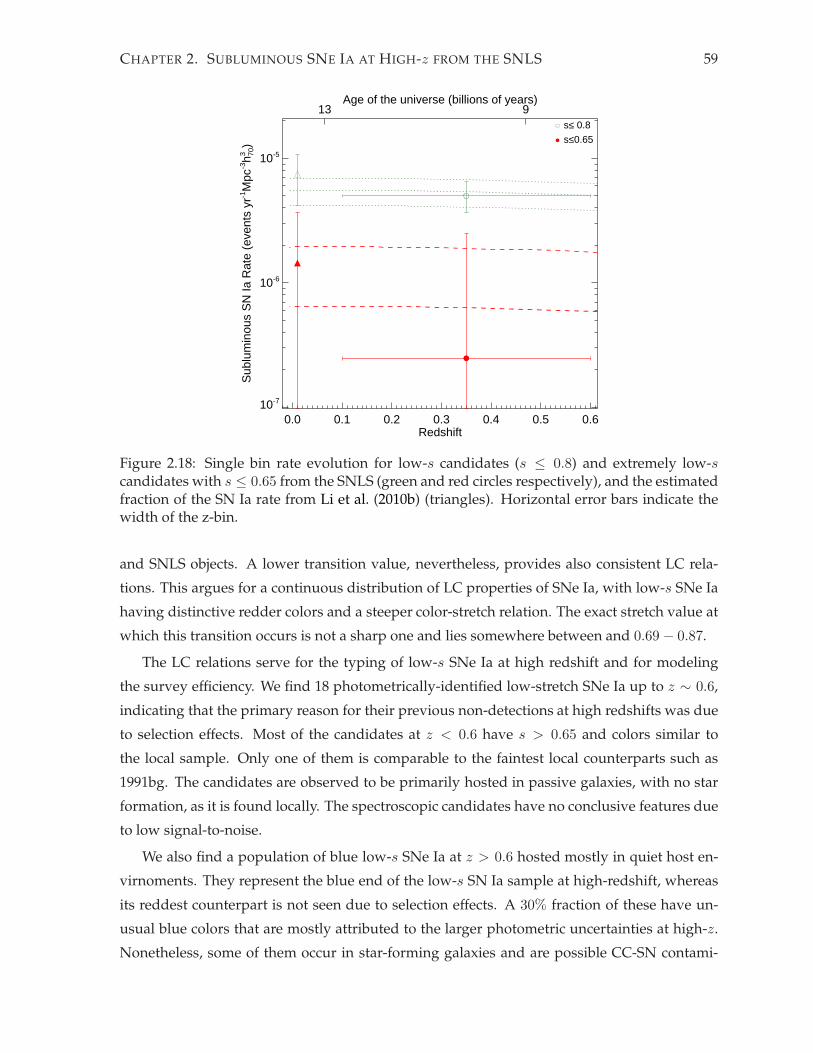
CHAPTER 2. SUBLUMINOUS SNE IA AT HIGH-z FROM THE SNLS 59
10-7
10-6
10-5
Sub
lum
inou
s S
N Ia
Rat
e (e
vent
s yr
-1M
pc-3h3 70
)
0.0 0.1 0.2 0.3 0.4 0.5 0.6Redshift
13 9Age of the universe (billions of years)
s≤ 0.8
s≤0.65
Figure 2.18: Single bin rate evolution for low-s candidates (s ≤ 0.8) and extremely low-scandidates with s ≤ 0.65 from the SNLS (green and red circles respectively), and the estimatedfraction of the SN Ia rate from Li et al. (2010b) (triangles). Horizontal error bars indicate thewidth of the z-bin.
and SNLS objects. A lower transition value, nevertheless, provides also consistent LC rela-
tions. This argues for a continuous distribution of LC properties of SNe Ia, with low-s SNe Ia
having distinctive redder colors and a steeper color-stretch relation. The exact stretch value at
which this transition occurs is not a sharp one and lies somewhere between and 0.69 − 0.87.
The LC relations serve for the typing of low-s SNe Ia at high redshift and for modeling
the survey efficiency. We find 18 photometrically-identified low-stretch SNe Ia up to z ∼ 0.6,
indicating that the primary reason for their previous non-detections at high redshifts was due
to selection effects. Most of the candidates at z < 0.6 have s > 0.65 and colors similar to
the local sample. Only one of them is comparable to the faintest local counterparts such as
1991bg. The candidates are observed to be primarily hosted in passive galaxies, with no star
formation, as it is found locally. The spectroscopic candidates have no conclusive features due
to low signal-to-noise.
We also find a population of blue low-s SNe Ia at z > 0.6 hosted mostly in quiet host en-
virnoments. They represent the blue end of the low-s SN Ia sample at high-redshift, whereas
its reddest counterpart is not seen due to selection effects. A 30% fraction of these have un-
usual blue colors that are mostly attributed to the larger photometric uncertainties at high-z.
Nonetheless, some of them occur in star-forming galaxies and are possible CC-SN contami-

CHAPTER 2. SUBLUMINOUS SNE IA AT HIGH-z FROM THE SNLS 60
nants (<∼ 10%). Alternatively we speculate that they could represent a different set of objects
that evolve rapidly but have bluer colors than typical low-s SNe.
We calculate a rate evolution of low-s SNe Ia as a function of redshift and the results indi-
cate a steady or slightly decreasing trend up to z = 0.6. We correct the rates at z > 0.6, where
our sample is incomplete, and find the evolution to be different from the increase of the nor-
mal SN Ia population. The missclassification of CC-SNe as SNe Ia (or different unknown blue
high-z transients) is an important source of systematics in the rate measurements. This would
overestimate the rate and should become larger with redshift, so that the effect of a decreasing
rate would be even stronger. The main findings of this study are therefore not influenced by
contamination.
An A-component model, proportional to just the mass of the galaxy, is sufficient to fit
the rate. This is expected as most of the candidates are hosted in passive galaxies with low
star formation. Low-s SNe Ia are therefore coming from an evolved population (in massive
galaxies) which corresponds to a long DTD, and could correlate with other properties such
as metallicity. Alternatively, they can arise from dynamical processes as found in globular
clusters, which congregate around large passive galaxies. The rate predicted by those events
would be roughly constant in time, although the absolute number is different by several orders
of magnitude.
As shown in Howell et al. (2007), this has consequences for cosmological studies because
the relative proportion of low to high stretch SNe Ia evolves at high redshift. The present study
supports their findings at the extreme low-stretch end of the population. We find that A + B
models have an A-component with ∼ 30% coming from the low-s population.
Studies of the DTD of different scenarios help constrain progenitors masses and models,
as well as the conversion efficiency of WDs into SNe Ia. The model of Strolger et al. (2010)
fitted to our data agrees with a Gaussian distribution centered around τ ≃ 5 − 6 Gyr, but
is not very constraining. The explosion fraction for those models is ν ∼ 10−3 − 10−4 low-s
SNe Ia per M⊙, an order of magnitude lower than for normal-s objects. These results again
argue for the low-s being part of a delayed component. Low-s SNe Ia, together with other
long delay SNe Ia of higher-s, could come from a separate progenitor channel. Although both,
the SD and DD, scenarios can produce delayed SNe Ia, the merger of two low-mass WDs
producing a sub-Chandrasekhar explosion seems more favorable to produce faint SNe in old
stellar environments. Meng et al. (2011) show that the merger of equal-mass WDs can give rise
to subluminous explosion with long enough delay-times, depending on the treatment of the
common envelope phase. Nevertheless, they argue that this scenario could only account for
1% of all SNe Ia, so that other mechanisms would be necessary to explain our 7-22% sublumi-
nous fraction.

CHAPTER 2. SUBLUMINOUS SNE IA AT HIGH-z FROM THE SNLS 61
Finally, future surveys should be able to determine the rate evolution of low-s much bet-
ter and to higher redshifts where the systematic errors in this study become more significant.
Spectroscopic redshifts of high-z low-s SNe Ia are essential for this and could provide ad-
ditional hint on their properties and their evolution. Further comparison of different SN Ia
populations will give clues to understand the formation and explosion mechanisms.
Chapter 3
The Rise-Time of Normal and
Subluminous Type Ia Supernovae
3.1 Introduction
Type Ia supernovae (SNe Ia) are believed to be very bright explosions of carbon-oxygen white
dwarfs (WDs) in binary systems that undergo thermonuclear runaway. Despite this consen-
sus, the nature of the companion and explosion mechanism are under debate. The enormous
energy release of a SN Ia takes around 2 weeks to peak in the optical. During this early phase
of the SN, when the luminosity rises to maximum, fundamental aspects of the explosion, and
possibly of the progenitor, are revealed to the observer. The spectroscopic presence of in-
termediate mass elements such as Silicon, between carbon-oxygen and iron-peak elements,
for instance, suggests incomplete burning from a subsonic deflagration component in the ex-
plosion (Filippenko 1997; Mazzali et al. 2007). A subsequent delayed detonation is typically
favored to account, among others, for the energy output of SNe Ia (Khokhlov 1991; Yamaoka
et al. 1992; Woosley & Weaver 1994).
The radioactive decay of the 56Ni synthesized in the explosion powers the lightcurve of
SNe Ia (Truran et al. 1967; Colgate & McKee 1969). It is thought that the variety in the amount
of 56Ni gives rise to most of the scatter in SN Ia luminosities. Values of 0.4 − 0.8M⊙ of 56Ni
result in “normal” SNe Ia. “Subluminous” or 1991bg-like objects, very faint and fast evolv-
ing SNe Ia, are produced by small amounts of 56Ni: 0.07 − 0.17M⊙ (Filippenko et al. 1992b;
Leibundgut et al. 1993). Slowly evolving and very bright SNe, such as 1991T are generated
by 0.85 − 1.1M⊙ of 56Ni (Phillips et al. 1992). In this framework, the duration from explosion
until maximum light, known as the rise-time, is partly determined by the amount of 56Ni (e.g
Arnett 1982; Shigeyama et al. 1992; Branch 1992; Khokhlov et al. 1993; Hoeflich et al. 1993;
Domınguez et al. 2001).
62
CHAPTER 3. THE RISE-TIME OF NORMAL AND SUBLUMINOUS TYPE IA SUPERNOVAE 63
The picture of the early behavior of SNe Ia has greatly benefited from the advent of im-
proved aspherical and multi-dimensional simulations of delayed detonations (e.g Bravo &
Garcıa-Senz 2008; Kasen et al. 2009; Maeda et al. 2010; Roepke et al. 2010). These authors show
that the quantity of 56Ni synthesized in the explosion that powers the lightcurve depends pri-
marily on a single parameter that can be characterized by the density at which the supposed
transition from deflagration to detonation in the delayed detonation framework occurs. If
the amount of burning in the deflagration phase is very large (due to, for example, numer-
ous symmetric sparks), the transition density is low and the detonation produces less 56Ni.
Nevertheless, other factors like the metallicity could affect the luminosity to second order (e.g
Timmes et al. 2003; Gallagher et al. 2008; Howell et al. 2009; Neill et al. 2011; Bravo et al. 2010).
Hoflich et al. (2010), for example, predict that a dependence of the early lightcurve on the C/O
ratio of the progenitor (determinedmainly by the progenitor main-sequence mass) potentially
affects the slope of the rise behavior at epochs earlier than 5 days before maximum.
Beyond the physics of the explosion, the rise-time study of SNe Ia can directly provide
information on the progenitor system. Kasen (2010) suggests that in the single degenerate
(SD) scenario, where a WD accretes material from a main-sequence or a red giant, the early
phase of the lightcurve can be affected by the interaction of the companion star with the SN
shock, particularly at shorter wavelengths. The magnitude depends on the observing angle,
as well as on the size and separation of the companion, and can be directly tested with well
sampled early rise-time data. In the double detonationof sub-Chandrasekhar mass WDs, Fink
et al. (2010) predict faster rise-times for brighter and slowly declining SNe Ia. They also show
that models with additional radioactive decay of other short-lived nuclei like 52Fe and 48Cr
contribute and magnify the early epoch output of SNe Ia.
Thesemodels suggest that the lightcurve parameterization of SNe Ia could need additional
corrections besides the standard width-luminosity –and color-luminosity as well as the recent
host mass-luminosity (Sullivan et al. 2010; Kelly et al. 2010), especially at early epochs. The in-
clusion of secondary parameters that correlate with luminosity may provide an improved cali-
bration of SNe Ia as distance indicators for cosmological studies. On the other hand, secondary
parameters might not affect the luminosity directly but still be very important to understand
the SNe Ia themselves.
Subluminous SNe Ia are an extremely faint population with redder colors. Standard sce-
narios do not reach the very faint explosions of subluminous SNe Ia and cannot reproduce
their Fe- and Si-composition. Pakmor et al. (2010) propose a merger system of two WDs of
similar masses (≃ 0.9M⊙) that is able to account for the low 56Ni mass of ≃ 0.1M⊙. These
objects are useful to understand the amount of 56Ni needed to power a lightcurve, and to in-
vestigate possible secondary effects. As subluminous SNe Ia are preferentially found in older,

CHAPTER 3. THE RISE-TIME OF NORMAL AND SUBLUMINOUS TYPE IA SUPERNOVAE 64
more metal-rich stellar populations (Hamuy et al. 1996a; Howell 2001; Gonzalez-Gaitan et al.
2011), they also offer an opportunity to study metallicity effects on the amount of 56Ni pro-
duced.
The early epoch study, however, requires good early sampling of SN lightcurves. Modern
rolling surveys like the Sloan Digital Sky Survey (SDSS) and the Supernova Legacy Survey
(SNLS) have a better cadence and provide very well sampled pre-maximum lightcurve data,
even of SNe discovered much later. Comparing fiducial stretch-corrected rise-times measured
from different groups is an extremely difficult task, particularly because of the rather arbitrary
definition of a fiducial, or, s = 1 template. Ideally, the study of several SN Ia populations, be
it at varying redshift or host environment for instance, should be done with the same tech-
niques and templates. Previous studies include the pioneering work by Riess et al. (1999b)
who found a B-band fiducial rise-time of 19.5 ± 0.2 days using combined nearby data −10
days before maximum. Aldering et al. (2000) find no evidence of evolution in SN Ia rise-time
and Conley et al. (2006, hereafter C06) confirmed this by calculating the rise-time of the low-z
data compared with higher-z from the SNLS (z < 0.9) finding consistent rise-times, 19.58+0.22−0.19
for the nearby and 19.10+0.18−0.17(statistical)±0.2(systematic) for the SNLS. Strovink (2007) found
a fiducial rise-time of 17.44 ± 0.39 days with an algorithm that avoids external templates and
fits smooth functions to the photometric data directly. Furthermore, they found individual
rise-times in a bimodal distribution around 18.81 ± 0.36 days and 16.64 ± 0.21 days. Hayden
et al. (2010b) propose a new parameterization of the lightcurve: they divide it into a rising and
a falling component, and find a stretch-corrected rise-time of 17.38±0.17 days for the SDSS, re-
jecting the bimodal distribution of Strovink (2007). They also find evidence for a faster stretch-
corrected rise-time in slow decliners. Hayden et al. (2010a) and Bianco et al. (2011) go further
to constrain the SD models of Kasen (2010) and have largely ruled out red giant companions.
None of the previous studies have included subluminous SNe Ia. In this work, we make
use of the large, homogeneously observed, but intrinsically heterogeneous SN Ia sample ob-
tained by the SNLS, in particular of the photometric group of low-stretch (s ≤ 0.8) objects
found in Gonzalez-Gaitan et al. (2011). We investigate the stretch-corrected rise-time behavior
of different SN Ia stretch populations to look for any secondary variations in the lightcurve
besides the standard width-luminosity relation. We study the importance of different tem-
plates and lightcurve fitting techniques on the stretch-corrected final rise-time calculations.
For proper comparison with other samples, we also analyze nearby and SDSS data with our
own techniques. The paper is organized as follows: In § 3.2 we present the rise-time parame-
terization used in our study, in § 3.3 we introduce the data we used, its analysis follows in § 3.4
and comparisons between subluminous SNe Ia and other populations, as well as to previous
studies are presented in § 3.5. We conclude in § 3.6.
CHAPTER 3. THE RISE-TIME OF NORMAL AND SUBLUMINOUS TYPE IA SUPERNOVAE 65
3.2 Rise-time fit
3.2.1 Lightcurve parameterization
We follow a similar approach to C06 to measure the common stretch-corrected rise-time of our
combined SN Ia sample data. We call this stretch-corrected rise-time a “fiducial” rise-time.
Different SNe Ia are corrected for lightcurve (LC) shape and normalized to peak flux, after
expressing all data in the same filter – normally B – via K-corrections. For the K-corrections,
we use the appropriate spectral energy distribution (SED) based on the epoch, SN’s redshift
and LC parameters such as stretch and color. For restframe epochs (corrected by dividing by
(1 + z)) before explosion, where the flux is generally zero, the K-corrections only include the
redshift term correction: −2.5 log(1 + z) (Nugent et al. 2002). Due to the small number of low-
stretch SNe Ia available, our study of the rise-time focuses on the average properties of the
aggregate stretch-corrected LCs, instead of individual rise-times.
The LC fitter used throughout this study is a modified version of the SiFTO algorithm
(Conley et al. 2008; Guy et al. 2010) that uses SED templates to model SN Ia LCs. The SED
sequence has been trained with low-z and SNLS data (Conley et al. 2008) and descends from
the spectral sequence of Hsiao et al. (2007). The LC is parameterized with a single time-axis
stretch parameter in the restframe B-band, sB . Each observed filter is stretched differently
according to a relation between the wavelength and sB (Conley et al. 2008). The modified
fitter also workswell for subluminous objects (Gonzalez-Gaitan et al. 2011, hereafter G11). The
same SEDs are used to K-correct all data to the restframe. Observed epochs are transformed
to effective dates, τ , by τ = (t − t0)/s(1 + z), where t0 is the date of maximum flux in the
restframe B-band and z is the redshift.
The LC fits normally use all available photometry, including the early time. In order not
to affect the rise-time analysis, we fit the LC and calculate stretch with only photometry past
a certain phase, i.e. τt < τ < 35 days. We call this the “core” LC. The transition value from
rise-time to core LC, τt, considered here ranges from −10 to −8 days (see § 3.4.5). One can also
use other LC parameters based uniquely on post-maximum data, such as ∆m15 (Phillips 1993;
Phillips et al. 1999). Alternatively, Hayden et al. (2010b, hereafter H10) suggest a two-stretch
approach for dividing the LC fit around the epoch of maximum light τ0. If f(t) is the flux, we
have:
f(t) =
f0 F ((t − t0)/sr) if t < t0
f0 F ((t − t0)/sf ) if t > t0
(3.1)
where f0 is the flux at peak (which is the same for both parts of the LC), F (t) is the fiducial

CHAPTER 3. THE RISE-TIME OF NORMAL AND SUBLUMINOUS TYPE IA SUPERNOVAE 66
(s = 1) flux of the template, and sr, sf are the rise and fall stretches, respectively. This means
that for the two-stretch technique, the epoch is given by τ = (t−t0)/sr(1+z) for pre-maximum
data and by τ = (t−t0)/sf (1+z) for post-maximum data. In this paper, we use both the single-
and two-stretch parameterizations to fit the LCs of SNe Ia.
3.2.2 Rise-time parameterization
To study the rise-time, we adopt the description used by Riess et al. (1999b); Aldering et al.
(2000); Goldhaber et al. (2001) and C06. If τ is the LC phase and tr is the fiducial rise-time of a
s = 1 SN that we want to constrain1, we have for the flux:
f(τ) = a(τ + tr)n + b, (3.2)
for τ > tr and b at earlier epochs. Normally, the nuisance parameter b should be zero, but
we investigate possible photometric subtraction errors that could systematically shift fluxes
up or down (see § 3.4.6). a is the slope of the rise and is another nuisance parameter in the
fit. The quadratic form, n = 2, is motivated by the characteristic expansion of a hot object in
the Rayleigh-Jeans tail of the SN Ia SED at early times in the B- and V -filters. The flux is pro-
portional to the temperature and to the radius squared, the latter in a homologous expansion
(r ∝ vτ ) depending linearly on the velocity of the expansion: f ∝ r2T ∝ v2(τ + tr)2T , where r
is the radius, v the rise “speed” and T the temperature. Since ∆T/T is almost constant obser-
vationally, and ∆v/v is also close to constant at early epochs, then f ∝ (τ + tr)2. Although past
studies agree that this quadratic model fits the rise-time behavior quite well, small variations
among SN Ia species are possible, not only for the rise-time tr but also for the power n of the
rise. We therefore investigate such variations as well (see § 3.4.7).
3.2.3 56Ni radioactive decay
The radiated luminosity of a SN Ia is powered by the radioactive decay of 56Ni through 56Co
to 56Fe (Arnett 1982; Arnett et al. 1985; Branch 1992). At peak, this energy is still trapped in
nickel and is slowly released by its radioactive decay (Nugent et al. 1995):
Lbol = γS(τr)MNi, (3.3)
1Note that we use tr for the average fiducial rise-time and τr for the individual rise-time of each SN uncorrectedfor stretch

CHAPTER 3. THE RISE-TIME OF NORMAL AND SUBLUMINOUS TYPE IA SUPERNOVAE 67
where MNi is the mass of 56Ni, γ ∼ 1.2 is the ratio of bolometric to radioactivity luminosities
for normal SNe Ia, and S is the luminosity from radioactivity per unit nickel mass given by:
S =(
6.31 e−τr/8.8 + 1.43 e−τr/111)
× 1043 erg s−1 M−1⊙ . (3.4)
This comes from the characteristic decay times of 56Ni and 56Co of 8.8 and 111 days, re-
spectively, with mean energy release per decay of 1.71MeV and 3.76MeV. Therefore, by mea-
suring the individual rise-time τr and bolometric luminosities Lbol of SNe Ia, we can estimate
the amount of 56Ni synthesized in the explosion under the assumed model. Variations in the
amount of 56Nimass produced in the explosion will lead to changes in the rise-time for a fixed
peak brightness (Contardo et al. 2000).
The value of γ is near unity but could in principle vary slightly depending on the 56Ni
mass, i. e. for large nickel masses, the radioactivity energy released above the photosphere
will escape directly instead of remaining trapped, leading to lower values of γ. In the absence
of a model for its variation, we assume γ = 1.2 ± 0.2 (Nugent et al. 1995) and propagate this
uncertainty in our calculations.
3.3 Data
3.3.1 SNLS
The five-year (2003-2008) Supernova Legacy Survey took advantage of the MegaCam wide-
field imager (Boulade et al. 2003) to observe supernovae, as part of the Canada-France-Hawaii
Telescope (CFHT) Deep Synoptic Survey. It used a rolling search technique suited for full
coverage of the LC, including early-time, by imaging every 3-4 days (2-3 days in SN restframe)
four fields in four different bands gMrM iMzM , which are similar to the filter system ugriz of
the SDSS (Smith et al. 2002). The SNLS had two independent photometric reconstructions
based in Canada and France (Guy et al. 2010). We use the French photometry here, as in the
SNLS cosmological analyses (Guy et al. 2010; Conley et al. 2011).
C06 used 73 spectroscopically confirmed normal SNe Ia for their rise-time study. Here,
we use 30 photometrically identified low-stretch (s ≤ 0.8) SNe Ia and 221 normal SNe Ia
(Gonzalez-Gaitan et al. 2011; Perrett et al. 2011) at 0.1 ≤ z ≤ 0.7 to study the respective stretch-
corrected rise-times and compare them. The photometric candidates went through a selection
process that ensured proper redshift and stretch estimation. As part of the selection criteria
to constrain the stretch, we require here good lightcurve sampling, particularly enough early
data. For this, we re-fit for stretch using only data after τt, to ensure the lightcurve shape
(stretch) is not affecting our rise-time estimation. We require at least two data points within

CHAPTER 3. THE RISE-TIME OF NORMAL AND SUBLUMINOUS TYPE IA SUPERNOVAE 68
τt < τ < 0 days of restframe B-bandmaximum. The restframeB-band for these objects will be
mostly mapped by rM (and somewhat by iM ). The lightcurves must also have a good SiFTO
fit with a total reduced chi-squared, χ2ν , better than 3.0. Additionally, we require that the
error in the determination of the peak epoch be less than 0.7 days (1.2 days for the two-stretch
parameterization, as shown in section 3.4.2). For the rise-time region fit, SNe Ia are required
to have data prior to −10 days. These cuts reduce the sample to 134 SNe, of which 12 have
s ≤ 0.8.
In our dataset, 35% of the low-s and 74% of the normal SNe Ia have a spectroscopic red-
shift. The effect of having uncertain photometric redshifts can lead to considerable errors
propagated in the K-corrections as well as in the effective dates τ of each SN, ultimately af-
fecting the rise-time fit. Throughout this study, photometric redshifts are used in the same
way spectroscopic redshifts are, but a proper inclusion of their errors is analyzed in § 3.4.1.
3.3.2 Low-z and SDSS
Table 3.1: Nearby objects used in the rise-time calculation. Name (column 1), redshift (col-umn2), single-stretch (column 3), 2-s rise- and fall-stretch (columns 4 and 5), and source (col-umn 6) are presented.
Name Redshift Stretch Rise-Stretch Fall-Stretch Source
SN1990n 0.0034 1.07 1.18 0.96 Lira et al. (1998)SN1994ae 0.0043 1.05 1.09 1.03 Riess et al. (2005),Altavilla et al. (2004)SN1997bq 0.0094 0.91 1.05 0.81 Jha et al. (2006)SN1998aq 0.0037 0.97 1.10 0.90 Riess et al. (2005)SN2000e 0.0048 1.06 1.28 1.00 Valentini et al. (2003); Tsvetkov (2006a)SN2001el 0.0039 0.96 1.12 0.91 Krisciunas et al. (2003)SN2001v 0.0150 1.09 1.22 1.05 Hicken et al. (2009)SN2002bo 0.0042 0.94 1.02 0.93 Krisciunas et al. (2004a)
SN2003du 0.0064 1.00 1.04 1.00Anupama et al. (2005),Stanishev et al.(2007),Leonard et al. (2005)
SN2004fu 0.0092 0.90 0.99 0.84 Tsvetkov (2006b); Hicken et al. (2009)
SN2005cf 0.0064 0.98 1.03 0.96Pastorello et al. (2007c),Wang et al.(2009b),Hicken et al. (2009)
SN2005mz 0.0176 0.63 0.91 0.53 Hicken et al. (2009)SN2006cp 0.0223 1.05 1.11 1.02 Hicken et al. (2009)SN2006gz 0.0237 1.22 1.30 1.19 Hicken et al. (2007)SN2006le 0.0174 1.08 1.10 1.05 Hicken et al. (2009)SN2007af 0.0055 0.94 1.07 0.91 Hicken et al. (2009)
To test our techniques, we also analyze available low-z rise-time data (see Table 3.1), as
well as the SDSS-II SNe Ia from Holtzman et al. (2008). We can thus compare our results to
low redshift to study any evolutionary effects. We cannot provide a comparison of our low-s

CHAPTER 3. THE RISE-TIME OF NORMAL AND SUBLUMINOUS TYPE IA SUPERNOVAE 69
stretch-corrected rise-time analysis to nearby ones, as published early data for nearby s ≤ 0.8
are scarce. The cuts applied to the SNLS are also used for the SDSS-II and low-z data, i. e. at
least two data points in restframe B-band at τt < τ < 0 days, and at least one point before τt.
3.4 Analysis
3.4.1 Rise-time calculation
To make a combined rise-time study of all SNe Ia in each sample, we process each lightcurve
as described in § 3.2.1. We then take the restframe B-fluxes of the low-stretch SNe Ia and
overlay them on a single plot, as shown in Figure 3.1. For the rise-time region, we use early
data, before a characteristic transition epoch τt = −10 days to fit it to themodel of Equation 3.2
(see Figure 3.2). Minimizing the χ2 of the best fit model with respect to the data provides the
best stretch-corrected rise-time. The choice of the transition epoch used affects the fit, as will
be shown in § 3.4.5. We perform an iterative outlier rejection (similar to C06) to discard any
data points that strongly deviate from the fit according to Chauvenet’s criterion (Taylor 1997).
For the total sample, this corresponds to 3.4σ and discards 25 (out of 449) data points, but does
not affect the final fit. It is tempting to argue that some of the points in Figure 3.2 for the lo-s
are above the fit (and template) and could provide evidence for interaction with a companion,
as in the model of Kasen (2010). This is hard to test with the available dataset but a red giant
companion has been rejected by Bianco et al. (2011) for the normal-s population.
The early time fit of the aggregate LC, nevertheless, does not take into account uncertainties
in the SN fit parameters and the photometric redshift. Errors in the redshift estimate induce
small changes in stretch (G11). Additionally, the use of a common SED for the LC fit as well
as for the K-corrections introduces strong correlations, as do the uncertainties of maximum
date and stretch of each SN fit. We handle these by shifting the photometric redshift according
to its error (for those SNe Ia with photo-z) in a Monte Carlo (MC) fashion. For each new
redshift a corresponding fit provides the new LC parameters (stretch, date of maximum and
flux scales) and their respective errors (and covariance matrix). These values and errors, in
turn, are used to generate a new set of random LC values (for SNe with and without photo-
z) that determine the model SED for each epoch. The K-corrections are recalculated for the
new set of redshift and LC parameters. For each of these realizations we fit the rise-time data
of all SNe to the model and get the best fiducial, stretch-corrected rise-time tr and slope a,
respectively. The final values are drawn from the median of all realizations combined. The
statistical uncertainties in the parameters are given by the 1σ uncertainties in the distribution
(see Figure 3.3). The distribution is broader for low-s because of the smaller sample size,and

CHAPTER 3. THE RISE-TIME OF NORMAL AND SUBLUMINOUS TYPE IA SUPERNOVAE 70
−20 0 20 40 60 80Restframe Epoch
−0.2
0.0
0.2
0.4
0.6
0.8
1.0
1.2
Flu
x [a
rbitr
ary
units
]
−20 0 20 40 60 80
G11median
C06s≤0.8
−20 0 20 40 60 80Restframe Epoch
−0.2
0.0
0.2
0.4
0.6
0.8
1.0
1.2
Flu
x [a
rbitr
ary
units
]
−20 0 20 40 60 80
G11median
C06s>0.8
Figure 3.1: Overlaid B-band restframe lightcurves of low- (s ≤ 0.8) and normal-stretch (s >0.8) SNe Ia from the SNLS. These are K-corrected, flux normalized and scaled to s and (1 + z).The blue dotted line is the median of the flux points, the dashed violet line is the fiducial G11template used, whereas the red dot-dashed is the template used in C06.

CHAPTER 3. THE RISE-TIME OF NORMAL AND SUBLUMINOUS TYPE IA SUPERNOVAE 71
−24 −22 −20 −18 −16 −14 −12 −10Restframe Epoch
−0.2
0.0
0.2
0.4F
lux
[arb
itrar
y un
its]
−24 −22 −20 −18 −16 −14 −12 −10
C06median
G11fit
s≤0.8
−24 −22 −20 −18 −16 −14 −12 −10Restframe Epoch
−0.2
0.0
0.2
0.4
Flu
x [a
rbitr
ary
units
]
−24 −22 −20 −18 −16 −14 −12 −10
C06median
G11fit
s>0.8
Figure 3.2: Overlaid B-band restframe lightcurves of low- (s ≤ 0.8) and normal-stretch (s >0.8) SNe Ia from the SNLS in the early rise at τt < −10 days. Red squares are outliers from thefit (∼ 3.4σ). The solid black line is the best quadratic fit, the blue dotted line is the median ofthe flux points, the dashed violet line is the fiducial G11 template used, and the red dot-dashedis the C06 template.

CHAPTER 3. THE RISE-TIME OF NORMAL AND SUBLUMINOUS TYPE IA SUPERNOVAE 72
because the low-s sample includes more SNe with photometric redshifts, and hence larger
errors in z (see G11 for details).
15 16 17 18 19 20tr (days)
0
10
20
30
40
50
Ns>0.8s≤0.8
Figure 3.3: Distribution of 100 MC stretch-corrected rise-time fits to s ≤ 0.8 (filled orange)and s > 0.8 (empty blue) SNe Ia. The dashed and dotted lines represent the median for bothsamples.
Final rise-times for the SNLS, SDSS-II and nearby samples are shown in Table 3.2. The
different samples agree well with each other providing no evidence for evolution. This is
confirmed by the fiducial rise-time of the SNLS SNe Ia at z > 0.7. Rise-times for different
SNLS stretch populations after the primary LC-width, or stretch, correction are also consistent.
However, the data are also in agreement at a ∼ 1σ level with a secondary slight trend for
longer fiducial rise-times in fast decliners. High-stretch SNe (s > 1.0) have the shortest stretch-
corrected rise-times, ∼ 1σ shorter than mid-stretch SNe (0.8 < s ≤ 1.0), and low-stretch (s ≤
0.8) also seem to follow this trend. In the next sections, we investigate systematic effects that
could modify these results.
3.4.2 Comparison of single- and two-stretch fits
Here, we investigate differences arising from the parameterization of the LC in two pieces
(rising and falling) as in Equation 3.2.1, and as done in H10. We process our data by fitting
it with a 2-s model, and we find that the rise-stretch and fall-stretch are consistent within
the errors, although the average rise-stretch is slightly larger than the fall-stretch: 〈sr − sf 〉 =

CHAPTER 3. THE RISE-TIME OF NORMAL AND SUBLUMINOUS TYPE IA SUPERNOVAE 73
Table 3.2: Stretch-corrected rise-time fit results for the single- and two-stretch lightcurve fits(with τt = −10 days)
Sample NSN (1-s) tr(1-s) (days)∗ NSN (2-s) tr(2-s) (days)
∗
SNLS z < 0.7 134 17.02+0.19−0.26 87 16.92+0.38
−0.49
s ≤ 0.8 12 18.03+0.81−1.37 8 17.89+1.31
−2.33
0.8 < s ≤ 1.0 55 17.44+0.45−0.43 31 17.56+0.63
−0.77
s > 1.0 67 16.87+0.15−0.25 48 16.62+0.44
−0.58
SNLS z > 0.7 102 17.11+0.24−0.36 15 16.11+0.68
−0.77
Nearby 16 17.39+0.16−0.24 15 16.58+0.21
−0.27
SDSS-II 64 17.44+0.33−0.53 36 17.03+0.26
−0.40
0.8 < s ≤ 1.0 23 17.78+0.34−0.40 12 17.51+0.31
−0.68
s > 1.0 41 17.37+0.44−0.44 24 16.91+0.24
−0.48
*Statistical MC errors only
0.09 (RMS of 0.24). The mean rise-stretch is also larger than the stretch from the 1-s model,
〈sr − s〉 = 0.06 (RMS of 0.17) (see Figure 3.4). This can be explained as the day of maximum
gets pushed to later times by more than half a day, 〈t0(sr, sf ) − t0(s)〉 = 0.65 (RMS of 1.77).
The mean error in the peak date is much larger for the 2-s fits, 〈∆t0(sr, sf ) − ∆t0(s)〉 = 0.87
(RMS of 0.53) (see Figure 3.5). An incorrect estimate of the date of maximum has a direct effect
on the rise-time calculation. For our MC technique, in which the fit parameters are varied
according to their errors, large uncertainties in the peak epoch will affect the final rise-time
even more. Our initial cut of ∆t0 < 0.7 days rejects more than 80% of the 2-s fits of the SNLS
sample (40% for the 1-s fits), including all low-s objects and all z > 0.7 SNe Ia. We therefore
relax the cut to ∆t0 < 1.2 days for the 2-s fits.
We do not change our low-s definition for the 2-s fits to sr ≤ 0.8 as this would reflect only
the early part of the LC. If wewere to use the fall-stretch instead, some low-s candidates would
have even lower stretch values. Instead we note that most candidates have a mean 2-s stretch,
i. e. (sr + sf )/2, closer to the single-stretch: (sr + sf )/2 − s = 0.01 with 0.05 RMS, and use this
to separate the different stretch samples. This definition keeps most of the low-s candidates
and is the best overall description of the lightcurve.
With the new stretch values we derived for the 2-s fits, we repeat the procedure to esti-
mate the fiducial rise-time, using the rise-stretch instead of the single stretch values for the K-
correction and normalization of all pre-maximum epochs. We obtain shorter stretch-corrected
rise-times than the 1-s approach, about 1-2% for the different SNLS samples (5% for SNe Ia
at z > 0.7), but still within the uncertainties. The decrease in fiducial rise-time with the 2-s

CHAPTER 3. THE RISE-TIME OF NORMAL AND SUBLUMINOUS TYPE IA SUPERNOVAE 74
respect to the 1-s fit comes partially from the compensation for the higher rise-stretches mea-
sured.
The 2-s technique introduces new parameters in the fit, and we want to assess if an im-
provement is simply due to the increased complexity of the model, or if there is a real ad-
vantage in using it. To compare the two models, we use the Bayesian Information Criterion,
BIC = χ2 + f ln(N), a tool that gives weight to the number of parameters of the fit, f , as
well as the total data used, N (Schwarz 1978). By summing all the individual core LC fits
(−10 < τ < 35 days) of all SNe, we find that the 1-s fit gives a smaller BICvalue: BIC = 17405,
compared to the 2-s value: BIC = 19721 (the average χ2 per degree of freedom for the indi-
vidual 2-s fits is slightly better,⟨
χ2ν
⟩
= 1.44, than for the 1-s technique:⟨
χ2⟩
= 1.48), i. e. the
2-s technique did not lead to a better fit once the increase in parameters is taken into account.
If we only consider the rise portion of the lightcurve (for which we use the same quadratic
fit for both techniques, so that BIC is unnecessary), we obtain a slightly lower chi-square per
degree of freedom for the 1-s approach, χ2ν = 1.60, than for the 2-s fit: χ2
ν = 1.64. The SNLS
systematic uncertainties from different LC fits, 2-s and a newer SiFTO version different from
G11, are shown in Table 3.3.
Similar results are found for the SDSS and low-z samples. The core LC fits are better for
the 1-s fits whereas the early rise-time fit is better for the 2-s approach, according to the BIC
criterion. The average rise-stretch is larger than the fall-stretch (by 0.09 for the SDSS and 0.11
for the low-z sample) partly because of a mean shift in the peak date (of 0.45 and 0.40 days
for the SDSS and low-z, respectively). The mean errors in peak time are somewhat lower (0.69
for the SDSS and 0.21 for the nearby sample). The final rise-times obtained are comparable for
both techniques, although the low-z 2-s result is ∼ 1.5σ lower than its 1-s counterpart.
In the present study, we do not find a significant change in the rise-times of different sam-
ples for the two parameterizations considered: 1-s and 2-s, except for the nearby set for which
a ∼ 1.5σ difference is found. Our 2-s technique that is based on an adapted two-piece SiFTO
fitter provides more uncertain peak date estimates. Requiring accurate maximum epochs af-
fects the number of SNe we can use in the fit for the 2-s technique (see section 3.3). We find
that using only SNe with ∆t0 < 1.2 days is good enough for the fit but the number of objects
used is less than for the 1-s technique, even though we use a tighter criterium for that fitter of
∆t0 < 0.7 days.
Although the statistical analysis of the fiducial rise-time remains unchanged with the pa-
rameterization used, Figure 3.4 shows that rise- and fall-stretches in the 2-s technique do not
vary equally for different SNe. The linear fits show that lower-s SNe Ia tend to have larger
rise-stretches and shorter fall-stretches for their respective 1-s, a higher difference between the
two, as compared to higher-s SNe Ia. The slopes of rise- and fall-stretch are different by more

CHAPTER 3. THE RISE-TIME OF NORMAL AND SUBLUMINOUS TYPE IA SUPERNOVAE 75
than 3σ.
0.6 0.8 1.0 1.21s - stretch
0.4
0.6
0.8
1.0
1.2
1.42s
- s
tret
ch
srsf<sr,sf>
Figure 3.4: Comparison of rise- (light blue triangles) and fall-stretch (dark blue inverted tri-angles) for SNLS SNe Ia calculated with the two-stretch technique as a function of the single-stretch. The crosses are the mean of the rise- and fall-stretches. The lines are linear fits: solid(red) for the mean of rise- and fall-stretches (slope: 0.91 ± 0.08), dotted (light blue) for rise-stretch (slope: 0.72 ± 0.07) and dashed (dark blue) for the fall-stretch (slope: 1.09 ± 0.04).
3.4.3 Comparison of different templates
The template used in C06 descended fromNugent et al. (2002) and the early portionwas based
on a limited number of SNe Ia. Using this template to calculate the rise-time, we obtain 19.33
days, in agreement with the result obtained in C06 of 19.10 days.
The fiducial stretch-corrected SN Ia rise-time is dependent on the SED template used (see
Figure 3.6), in particular on the rather arbitrary definition of a s = 1 SN. This is especially
important when comparing rise-times from different sources, where various templates can
lead to different rise-times. A s = 1 SN is defined here as the mean stretch of the training
sample for the template we use, which is the same as in G11. If we correct rise-time of the
C06 template for the different s = 1 definitions, by comparing the fits directly (see Figure 3.7),

CHAPTER 3. THE RISE-TIME OF NORMAL AND SUBLUMINOUS TYPE IA SUPERNOVAE 76
-5 0 5 10t0(s)-t0(sr,sf)
0
10
20
30
40
N
-5 -4 -3 -2 -1 0 1∆ t0(s)-∆ t0(sr,sf)
0
20
40
60
80
N
Figure 3.5: Difference of peak date (upper) and peak date error (lower) calculated with the 1-sand the 2-s techniques for the SNLS sample

CHAPTER 3. THE RISE-TIME OF NORMAL AND SUBLUMINOUS TYPE IA SUPERNOVAE 77
Table 3.3: Stretch-corrected rise-time systematic uncertainties for the SNLS stretch samples:low-s (s ≤ 0.8), mid-s (0.8 < s ≤ 1.0) and high-s (s > 0.8) and differences between them
Systematic Rise-time tr (days) Difference ∆tr (days)
all low-s mid-s high-s low-s - mids mid-s - high-s
(s ≤ 0.8) (0.8 < s ≤ 1.0) (s > 1.0)
STANDARD 17.02+0.19−0.26 18.03+0.81
−1.37 17.44+0.45−0.43 16.87+0.15
−0.25 0.59+0.93−1.44 0.57+0.47
−0.50
LC-FIT
1-s new SiFTO 17.14 18.46 17.99 16.57 0.47 1.42
2-s 16.92 17.89 17.56 16.62 0.97 0.94
TEMPLATE
NEW (conley09f) 16.94 18.33 17.70 16.59 0.63 1.11
C06 (nugent05) 18.77 20.13 19.68 18.21 0.45 1.47
SALT2 18.16 19.13 18.77 17.57 0.36 1.20
TRANSITION EPOCH
τt = −8d 17.22 18.68 17.56 16.95 1.12 0.61
PHOTOMETRY
Fr phot, b = 0 17.21 17.96 17.40 16.96 1.02 0.44
Ca phot, free b 17.18 18.07 17.50 16.86 1.03 0.64
POWER LAW
n = 1.9 16.83 17.87 17.26 16.68 0.61 0.58
σtotsyst
+1.78−0.23
+2.24−0.22
+2.31−0.18
+1.35−0.45
+0.69−0.27
+1.24−0.13
*This template is based on an old limited SN sample and is not included in the final systematic error budget.
-20 0 20 40 60 80 100epoch
0.0
0.2
0.4
0.6
0.8
1.0
flux
C06 (nugent05)G11 (conley07h)NEW (conley09f)
salt2
-20 -18 -16 -14 -12 -10 -8epoch
0.0
0.2
0.4
0.6
0.8
flux
C06 (nugent05)G11 (conley07h)NEW (conley09f)salt2
Figure 3.6: Different SN Ia light-curve templates (inset of early portion on the right): C06 (solidblack), G11 (dotted blue), NEW (dashed red) and SALT2 (dot-dashed green).

CHAPTER 3. THE RISE-TIME OF NORMAL AND SUBLUMINOUS TYPE IA SUPERNOVAE 78
i. e. a s = 1 SN for the G11 template corresponds to a s = 1.03 for the C06 template, we then
obtain 18.77 days. This averaged correction partially accounts for the early wide behavior of
the C06 template (see Figure 3.2). The simple change of s = 1 definition is not sufficient to
fully compensate the effect of an incorrect early template, so that a longer stretch-corrected
rise-time is still obtained. We get similar long rise-times with the C06 template applied to the
2-s technique, indicating that this parameterization is not independent of the template used.
Newer templates trained with the well-sampled data of the SNLS, like the one used in G11,
or a more recent version trained with a larger sample (used for SiFTO in Guy et al. 2010), give
consistent rise-times after correction for the different s = 1 definition. Table 3.3 shows the
rise-times for different templates.
0.6 0.7 0.8 0.9 1.0 1.1 1.2sG11
−0.15
−0.10
−0.05
−0.00
0.05
0.10
0.15
s G11
−s o
ther
sNEW
sC06
Figure 3.7: Stretch comparison between lightcurve fits of the G11 template and other tem-plates: C06 (purple dots), and a more recent one NEW (red squares). The purple dashed andred dot-dashed lines are the averaged median in 0.05 stretch bins.
3.4.4 Comparison with SALT2
We investigate here the use of a different LC fitter, SALT2 (Guy et al. 2007). This fitter also
makes use of different templates from the ones presented in the previous section, so that we
are probing two systematics simultaneously.
In order to do this, we fit all SNe Ia with SALT2 in the range τ > −10 days. A direct com-
parison of their SiFTO stretch and X1 parameter from SALT2 is shown in Figure 3.8 through

CHAPTER 3. THE RISE-TIME OF NORMAL AND SUBLUMINOUS TYPE IA SUPERNOVAE 79
a linear fit. We calculate restframe, stretch-corrected epochs using the redshift and a corre-
sponding stretch (for each X1 parameter): τ = (t−t0)/s(X1)(1+z). Every data point matching
restframe B-band is K-corrrected by taking the SED for each restframe epoch based on Eq. 1
of Guy et al. (2007) with X0, X1 and color obtained from the SALT2 fit, and integrating it in
the appropriate filter at the proper redshift. We then fit the aggregate LC points of the early
rise (τ < −10 days) to the quadratic rise model.
-4 -2 0 2 4x1
0.7
0.8
0.9
1.0
1.1
1.2
stre
tch
Figure 3.8: Comparison of SiFTO stretch and SALT2 X1 for the SNLS SN Ia sample. The solidline represents the fit: st = a × X1 + b with a = 0.086 ± 0.026 and b = 0.997 ± 0.022.
Similarly, we take into account errors with a MC that shifts the fit parameters (zphot if
necessary, and τmax, X0, X1 and color) according to their covariance matrix, and re-calculate a
stretch from this, as well as a new K-correction for each point of each simulation. The mean of
all iteriations, the final fiducial rise-time we obtain for the normal-s population, is 18.16± 0.44
days. This is larger than ∼ 1.1 days than the standard SiFTO 1-s and 2-s rise-times. Although
the SALT2 template is different than the templates we use (see Figure 3.6), is is not as extreme
as the C06 template. Clearly, the use of the LC fitter also affects the measured rise-time and
is an important systematic. The differences between SN Ia populations are still consistent as
shown in Table 3.3 (under “template”, although this is a twofold systematic: “template” and
“LC-fit”).
3.4.5 Transition Epoch
The transition epoch is the minimum epoch used in the core LC fit and the maximum epoch
allowed in the early rise-time fit. Its value can affect the quality of the fit but also the resulting

CHAPTER 3. THE RISE-TIME OF NORMAL AND SUBLUMINOUS TYPE IA SUPERNOVAE 80
rise-time (and even the quadratic behavior of the rise). A higher value, like τt = −6 days,
increases the amount of data for the early-time fit, but the rise may no longer follow a simple
quadratic relation. Figure 3.9 shows that rise-time fits with different transition times and a
fixed power fit (quadratic n = 2) for the SNLS do not change much up to a maximum value of
τt ≃ −8 days, where the rise-time starts to diverge. We use here the standard τt = −10 days
used in other studies but add a systematic uncertainty to the rise-time based on the differences
at τt = −8 days (see Table 3.3).
-12 -10 -8 -6Transition Time τt (days)
16.5
17.0
17.5
18.0
Ris
e T
ime
t r (d
ays)
1s-fit
2s-fit
Figure 3.9: Stretch-corrected rise-time as a function of the transition epoch, the maximum dateallowed in the single- (black circles) and two-stretch (red squares) rise-time fits. The rise-timeerrors are the MC errors calculated as in § 3.4.1. The larger points at τt = −10days are thequoted fiducial rise-times of this study.
3.4.6 Zero scale b
Wrong photometric subtraction affects fluxes that are close to zero and strongly influences the
final stretch-corrected rise-time calculation. To study this systematic error, we add a nuisance
parameter, b, to the quadratic form (Eq. 3.2) that will absorb any general photometric error.
For a good photometry, we should obtain b values close to zero. In our study, we get b =
(−0.48+0.12−0.09) × 10−3, an off-zero value reflecting the large dispersion of the fluxes near zero
(median of 3.1 × 10⁻⁴ with 0.03 RMS) but small enough to represent a negligible effect on
the rise-time. Consistent rise-times are obtained with free/fixed b values for the photometry

CHAPTER 3. THE RISE-TIME OF NORMAL AND SUBLUMINOUS TYPE IA SUPERNOVAE 81
processed via the French and Canadian reconstructions, as seen in Table 3.3.
The importance of this parameter can be observed in Figure 3.10(a), in which different b
values in the range −0.05 < b < 0.05, or a 5% maximum shift of the normalized flux at peak,
result in rise-times shifted by several days. We emphasize therefore the importance of proper
photometry,well-sampled to dates even before explosion, to correctly calculate b and not affect
the rise-time.
3.4.7 Different rise power laws
Other parameters that could influence the fiducial rise-time behavior are a and the rise power
n in Eq. 3.2. We find a = (7.40+0.58−0.62) × 10−3 for the normal-s SNLS population (arbitrary
flux units) and an assumed n = 2 quadratic form. If we relax the quadratic rise assumption
and allow the power of the rise-time model to be free (a is free and b = 0), we obtain n =
1.92+0.31−0.37(stat). Rise-times fitted with this new power law are lower for all stretch populations
but consistent with their quadratic equivalents.
Figure 3.10(b) shows the relation between the assumed power-law, n, and the measured
stretch-corrected rise-time, tr for the normal SN Ia sample. A higher nmakes the LC rise faster.
In order to compensate for this, the duration of the rise to maximum of the fit becomes longer.
This effect has a high degree of degeneracy and correlation between the two fit parameters. A
very similar trend is observed for the different stretch samples. Furthermore, if the quadratic
form is relaxed for all populations, we obtain increasing power laws and rise time for higher-s
SNe (Table 3.4). This variation shows again the clear difference in the rise-time region for the
sub-samples of SNe Ia.
Table 3.4: Stretch-corrected rise-time and power-exponents fit results for the different stretchsamples in the SNLS
Sample tr(days)∗ n∗
SNLS 16.85+0.54−0.81 1.92+0.31
−0.37
High-s 17.89+0.77−0.98 2.66+0.44
−0.59
Mid-s 16.49+0.56−0.88 1.48+0.34
−0.37
Low-s 16.14+1.00−1.99 0.78+0.71
−0.71
*Statistical MC errors
Although the systematic uncertainty from this variation is also highly correlated with the
transition time, we still include it in the total systematic error budget.
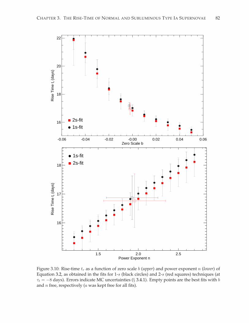
CHAPTER 3. THE RISE-TIME OF NORMAL AND SUBLUMINOUS TYPE IA SUPERNOVAE 82
-0.06 -0.04 -0.02 -0.00 0.02 0.04 0.06Zero Scale b
16
18
20
22
Ris
e T
ime
t r (d
ays)
1s-fit
2s-fit
1.5 2.0 2.5Power Exponent n
16
17
18
Ris
e T
ime
t r (d
ays)
1s-fit
2s-fit
Figure 3.10: Rise-time tr as a function of zero scale b (upper) and power exponent n (lower) ofEquation 3.2, as obtained in the fits for 1-s (black circles) and 2-s (red squares) techniques (atτt = −8 days). Errors indicate MC uncertainties (§ 3.4.1). Empty points are the best fits with band n free, respectively (a was kept free for all fits).

CHAPTER 3. THE RISE-TIME OF NORMAL AND SUBLUMINOUS TYPE IA SUPERNOVAE 83
3.5 Results and Discussion
The final fiducial rise-time, tr, for all SNe Ia in the SNLS calculated via the single-stretch
method is tr = 17.02+0.19−0.26(statistical)
+0.30−0.23(systematic). The statistical uncertainty represents
the 1σ distribution of the MC simulations and the systematic uncertainty comes from the dif-
ferent effects considered in the previous section (added in quadrature) and shown in Table 3.3.
This agrees with the value found via the two-stretch technique.
We find that the fiducial stretch-corrected rise-times are consistent for fast and slow de-
cliners, independently of different fit characteristics such as the template or lightcurve fitter.
Mid-stretch SNe Ia (0.8 < s ≤ 1.0) have a fiducial rise-time ∆tr = 0.57+0.47−0.50(stat)
+1.24−0.13(syst)
days longer than their high-stretch counterpart (s > 1.0), barely a ∼ 1σ result. With even
lower significance, low-stretch SNe Ia show a difference with respect to the high-stretch pop-
ulation of ∆tr = 1.16+0.82−1.39(stat)
+1.42−0.19(syst) days.
Although we do not measure individual rise-times, an estimate based on the stretch of
each object can be obtained from the fiducial rise-time. For the single-stretch case we do
τr,i = si × tr(s), where the subscript i denotes each individual SN and tr(s) is the fiducial
rise-time. Individual rise-times for the low-s population lie in the range of 10-14 days. For the
normal-s population, they lie in the range of 14-21 days. We plot them as a function of B-band
magnitude at maximum and SALT2X1 in Figure 3.11. One can see that as τr is calculated from
stretch, which correlates with X1, the rise-time follows the LC-shape quite closely, while there
is more scatter with maximum brightness.
3.5.1 Comparison to previous studies
As mentioned in § 3.4.3, the different definition of a fiducial s = 1 lightcurve across differ-
ent templates makes the comparison of stretch-corrected rise-times from several studies quite
difficult.
Having that in mind, recent studies (Strovink 2007; Hayden et al. 2010b), including the
present one, agree that the average rise-time of SNe Ia is shorter than previously thought. With
more data, better-sampled at early times, the new templates, as well as LC-fitting techniques,
provide evidence for a∼2 days shift in the average rise-time of SNe Ia with respect to previous
studies (Riess et al. 1999b; Conley et al. 2006), although the precise value is heavily dependent
on the definition of a fiducial s = 1 LC template.
Although we use the same technique as C06, the template they used was trained with
a handful of SNe Ia and consequently had a rise-time behavior to maximum quite different
from the current templates. Their rise-time is longer than the one we find here, even after
correcting for our s = 1 definition.

CHAPTER 3. THE RISE-TIME OF NORMAL AND SUBLUMINOUS TYPE IA SUPERNOVAE 84
−20.0 −19.5 −19.0 −18.5 −18.0 −17.5 −17.0MB
max
10
12
14
16
18
20
22
24τ r
nor−s
low−s
−3 −2 −1 0 1 2 3X1
10
12
14
16
18
20
22
24
τ r
Figure 3.11: Individual rise-times as a function of B-band magnitude at maximum and X1

CHAPTER 3. THE RISE-TIME OF NORMAL AND SUBLUMINOUS TYPE IA SUPERNOVAE 85
We also analyze the nearby and SDSS-II datasets with our same template and LC fitter.
H10 used a much larger SDSS-II sample (361 SNe) than used here (the 146 SDSS-II SNe from
Holtzman et al. 2008). Our SDSS-II fiducial rise-time agrees well with theirs. They argue that
the two-stretch technique presents a much better parameterization than a single parameter
approach. We do not agree with those findings, neither for the SNLS nor the SDSS and low-z
data. We attribute this to the use of a different fiducial LC template and fitter that differ in
the rise-time region from the ones they use (G11 and modified SiFTO vs MLCS2k2, Jha et al.
2007), in particular the stretch they calculate is not based on multiple bands. The Bayesian
Information Criterion for the core LC fits suggest that the inclusion of an additional parameter
to model SN Ia lightcurves does not provide a valuable improvement of the fit. The quadratic
fit of the early rise-time data, on the other hand, could benefit from such an independent
parameterization but does not alter the average rise-time results.
Based on our calculations of the fiducial rise-time for different samples across the redshift
range 0 < z < 1, we do not find evidence for a significant evolution in the early portion of
SN Ia lightcurves. Dividing the SNLS sample into three populations according to their stretch
values, we measure the average rise-times for each sub-group and find them to be consistent.
Although at low confidence, the data also agree with a trend of faster fiducial rise-times for
brighter and slowly declining SNe Ia after the primary stretch correction, for the SNLS and
SDSS-II. H10 obtained a similar trend for the individual rise-times of SDSS-II objects.
3.5.2 56Ni masses
In order to estimate the 56Ni masses, we need to calculate bolometric luminosities. We in-
tegrate the model SEDs for each SN across all observed bands. This omits the near-infrared
(NIR), which accounts for a substantial fraction of the bolometric luminosity, so we must ap-
ply a correction factor. In Howell et al. (2009) the IR percentage for normal SNe Ia is estimated
via integration of proper SEDs corrected for each SN in the region outside the observed spec-
trum, under some assumptions. For low-s SNe Ia, SEDs are not as fully sampled. We instead
use a very broad approximation based on the IR fraction found for SN1999by and SN2004eo
(Hoflich et al. 2002; Garnavich et al. 2004; Taubenberger et al. 2008): ∼ 15 − 25%. The fraction
is at least 5% higher than for normal SNe Ia. We use a standard 20 ± 10% value (and 10 ± 5%
for the normal-s) to calculate via Equations 3.3 and 3.4 the 56Ni mass.
In order to account for the errors in the LC parameters, we carry out this computation for
every realization of the LC data in the MC of § 3.4.1, and use the median LB of each SN to
calculate the final 56Ni masses, as shown in Figures 3.12 and 3.13. We also include the error
on the conversion factor γ, which can also slightly vary with 56Ni mass. The 56Ni masses
lie between 0.05-0.35 M⊙ for the low-s and 0.1-0.8 M⊙ for the normal-s populations. Our

CHAPTER 3. THE RISE-TIME OF NORMAL AND SUBLUMINOUS TYPE IA SUPERNOVAE 86
0.2 0.4 0.6 0.856Ni mass (MS)
0
10
20
30
40
N
1-s s>0.82-s s>0.81-s s≤0.82-s s≤0.8
Figure 3.12: Distribution 56Nimasses (solar units) for the normal-s (solid histograms) and low-s (filled histograms) SN Ia SNLS samples based on 1-s (black) and 2-s (red) fits. Vertical linesrepresent the mean for each case.
estimates are lower than typical values in the literature because of the lower rise-times. They
are similar for both parameterizations of the lightcurve (see Figure 3.14).
Figure 3.13 shows 56Ni masses as a function of the individual rise-times for all SN Ia. The
relation of Ni mass and rise-time is expected from the use of Arnett’s rule. The individual
rise-times are obtained from the fiducial rise-time and the individual stretches, so that 56Ni
mass also relates with stretch. The scatter of 56Nimasses is quite high at a given τr. This is due
the large range of bolometric luminosities as seen in the large distribution of MmaxB , as seen in
Figure 3.11.
One can also observe that, as the rise-time is more independent of stretch for the 2-s tech-
nique, there is a more diverse 56Nimass range for each stretch population. It may be beneficial
to divide the LC into separate regions, rise and fall, to disentangle the rise portion from the
primary width-luminosity driver, when studying early-time effects of SNe Ia.
3.5.3 Secondary lightcurve parameters
The need for secondary parameters to describe SNe Ia at early times, beyond the traditional
core LC parameter like stretch or ∆m15, would have important consequences for the under-
standing of SNe Ia. To the precision achieved in this study, these secondary effects in the early

CHAPTER 3. THE RISE-TIME OF NORMAL AND SUBLUMINOUS TYPE IA SUPERNOVAE 87
10 12 14 16 18 20 22 24τr (days)
0.0
0.2
0.4
0.6
0.8
1.0
56N
i mas
s (M
S)
low-smid-shigh-s
10 12 14 16 18 20 22 24τr (days)
0.0
0.2
0.4
0.6
0.8
1.0
56N
i mas
s (M
S)
low-smid-shigh-s
Figure 3.13: 56Ni mass as a function of individual rise-time for the single- (upper) and two-stretch (lower) techniques. The low-s (orange circles), mid-s (blue triangles) and high-s (lightblue squares) SNe Ia are indicated.
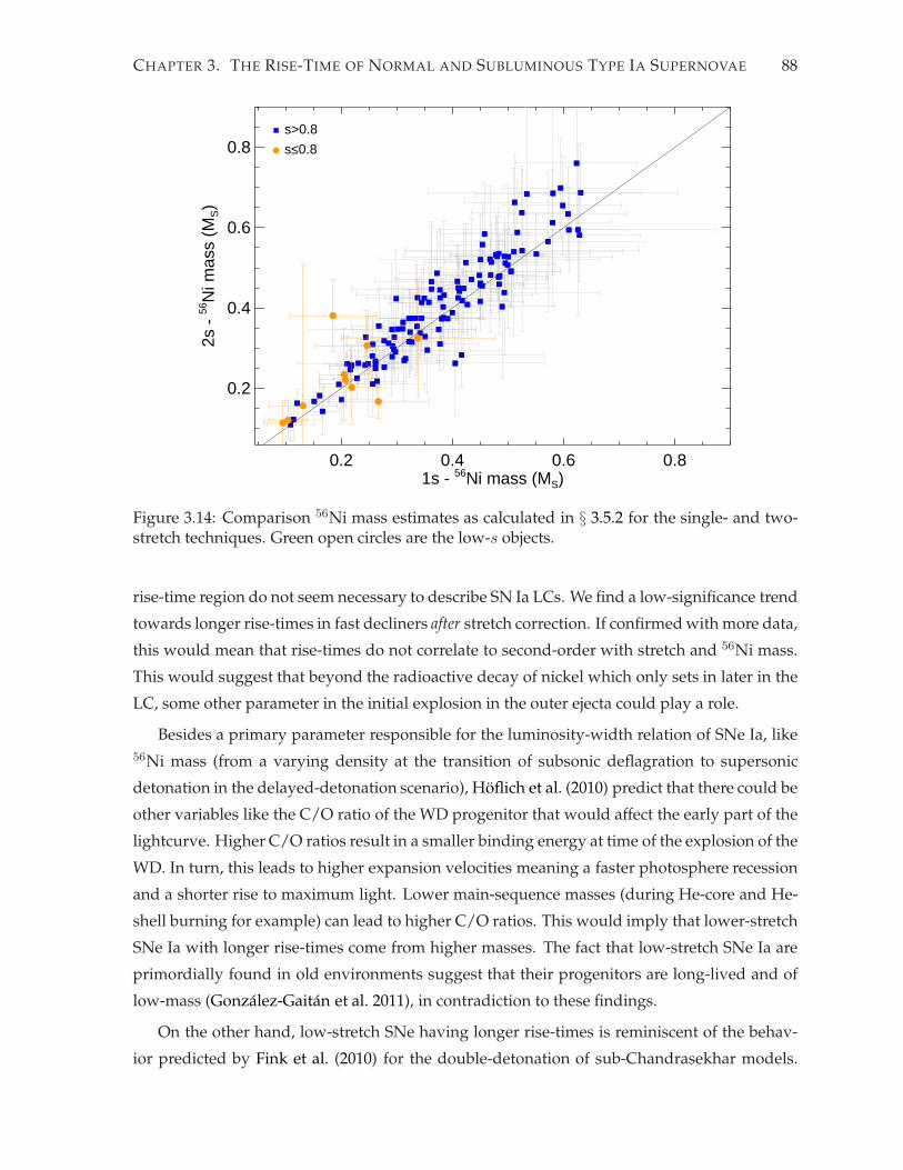
CHAPTER 3. THE RISE-TIME OF NORMAL AND SUBLUMINOUS TYPE IA SUPERNOVAE 88
0.2 0.4 0.6 0.81s - 56Ni mass (MS)
0.2
0.4
0.6
0.8
2s -
56N
i mas
s (M
S)
s>0.8
s≤0.8
Figure 3.14: Comparison 56Ni mass estimates as calculated in § 3.5.2 for the single- and two-stretch techniques. Green open circles are the low-s objects.
rise-time region do not seem necessary to describe SN Ia LCs. We find a low-significance trend
towards longer rise-times in fast decliners after stretch correction. If confirmedwith more data,
this would mean that rise-times do not correlate to second-order with stretch and 56Ni mass.
This would suggest that beyond the radioactive decay of nickel which only sets in later in the
LC, some other parameter in the initial explosion in the outer ejecta could play a role.
Besides a primary parameter responsible for the luminosity-width relation of SNe Ia, like
56Ni mass (from a varying density at the transition of subsonic deflagration to supersonic
detonation in the delayed-detonation scenario), Hoflich et al. (2010) predict that there could be
other variables like the C/O ratio of the WD progenitor that would affect the early part of the
lightcurve. Higher C/O ratios result in a smaller binding energy at time of the explosion of the
WD. In turn, this leads to higher expansion velocities meaning a faster photosphere recession
and a shorter rise to maximum light. Lower main-sequence masses (during He-core and He-
shell burning for example) can lead to higher C/O ratios. This would imply that lower-stretch
SNe Ia with longer rise-times come from higher masses. The fact that low-stretch SNe Ia are
primordially found in old environments suggest that their progenitors are long-lived and of
low-mass (Gonzalez-Gaitan et al. 2011), in contradiction to these findings.
On the other hand, low-stretch SNe having longer rise-times is reminiscent of the behav-
ior predicted by Fink et al. (2010) for the double-detonation of sub-Chandrasekhar models.

CHAPTER 3. THE RISE-TIME OF NORMAL AND SUBLUMINOUS TYPE IA SUPERNOVAE 89
The initial He-shell detonation on the WD surface can lead to a detonation of the CO core of
the WD. Varying WD masses (0.8-1.4M⊙), and with it their central core and shell densities,
give rise to a variety of 56Ni masses and burning products powering the lightcurve. Particu-
larly they find that brighter events have faster rise-times. This is because brighter explosions
produce more core 56Ni that expand faster with less opacity in the outer shells from iron-
group-elements created in the He-shell detonation. Their effect is anti-corrected with stretch,
which would indicate a primary correction rather than a secondary one. In this picture, the
lightcurve and the rise-time are directly related to the initial mass of theWD. Lower-massWDs
(of ∼ 0.8M⊙) have lower He-shell and CO core densities leading to a distribution of burning
products that give rise to slower rise-times for low-stretch SNe Ia. LowermassWDs producing
fast decliners would agree with the aforementioned observations of older host environments.
Another interesting feature of the predictions by Fink et al. (2010) is that the contribution
of other radioactive elements like 52Fe and 48Cr of short decay times can make the rise-time
longer. This is particularly true for subluminous SNe Ia, which in their models produce as
much as 20% of these radioactive nuclei, particularly 44Ti, which does not contribute to the
early lightcurve, but is known to be observed in the spectra as well. These yields are a direct
consequence of the initial He-shell detonation.
3.6 Conclusions
We have constructed aggregate restframe B-band LCs of a sample of spectroscopic and pho-
tometrically identified SNe Ia at z ≤ 0.7 from the SNLS. We obtain fiducial rise-times that
are consistent with measurements for the low-z and SDSS-II samples calculated here with the
same techniques. We extend our SNLS sample and show that there is no significant evolution
in the early portion of SN Ia lightcurves up to z = 1.0.
We find that the use of a two-stretch parameterization for the lightcurve fits of SNe Ia is
equivalent to the single-stretch parameterization. We confirm the consistency for the SDSS-II
and SNLS samples while the nearby set has a rise-time ∼ 1.5σ lower for the 2-s technique and
discrepant with all other calculated rise-times. The 2-s approach might be useful for detailed
studies of the early-rise time that reach higher precision than the one attained in this work. We
insist in the importance of proper lightcurve fitters with parameters that can take into account
earlier parts of the lightcurve (stretch vs ∆m15) and that include multi-band information, and
of templates trained with sufficient SNe with early time data.
We have compared the early region fits for different stretch population of the SNLS. We
find that the stretch-corrected rise-times are consistent within uncertainties for slow and fast
decliners. We extend this result to the lowest stretch objects. These findings are independent

CHAPTER 3. THE RISE-TIME OF NORMAL AND SUBLUMINOUS TYPE IA SUPERNOVAE 90
of systematics such as the maximum epoch allowed in the early time fits, as well as on the two
LC parameterizations assumed. The present study averages over samples which can have ob-
vious difficulties like the low statistics of the low-stretch population. At a low significance of
∼ 1σ, our results also agree with a trend for longer rise-times in fast declining SNe Ia. If these
indications are confirmed, then SN Ia explosions differ beyond a single parameter orchestrat-
ing the lightcurve of SNe Ia. Secondary parameters in the early rise region would be necessary
to fully model the lightcurves and could provide useful insights into SN Ia explosions. Such
an indication is also found for the SDSS-II, as in H10.
However, to the precision attained in this study, SNe Ia remain extremely homogeneous
all the way to very early times. One single lightcurve parameter, that possibly translates to
a unique physical variable, like the transition density of deflagration to detonation in the de-
layed detonation model, can account not only for the core lightcurves of SNe Ia, but largely
for the rise-time as well. The similarity of SN Ia lightcurves (after stretch-correcting) argue for
a real common origin, with subluminous SNe Ia at the extreme end of the population.
The fiducial rise-time we find translates into 56Ni masses of 0.05 − 0.90M⊙ for all SNe Ia
(and 0.05−0.35M⊙ for low-s SNe Ia). Although our assumed IR contribution to the bolometric
luminosity is uncertain, extremely low amounts of radioactive 56Ni seem enough to power a
faint SN Ia, less than that the amount found by Filippenko et al. (1992b); Leibundgut et al.
(1993). Our SNe with the lowest radioactive nickel yield even rival with peculiar extreme
objects such as the ones found by McClelland et al. (2010); Kasliwal et al. (2010); Poznanski
et al. (2010), and pose a challenge to explosion models.
Such weak explosions seem unlikely to be the outcome of a runaway of a WD near the
Chandrasekhar mass. Sub-Chandrasekhar models have been indeed a natural way of explain-
ing subluminous SNe Ia (e. g. Livne 1990; Woosley & Weaver 1994), and possibly all SNe Ia
(Fink et al. 2010; Sim et al. 2010; van Kerkwijk et al. 2010). Located in passive environments
that are characteristic of old populations, low-mass WDs seem a promising progenitor of sub-
luminous SNe Ia. With recent rejections of a high fraction of RG donors (Hayden et al. 2010b;
Bianco et al. 2011), a double degenerate merger leading to the sub-Chandrasekhar explosion
of a low-mass WD with very low 56Ni yield appears increasingly plausible. If SNe Ia share a
common explosion and progenitor mechanism, a varying progenitor WD mass could possi-
bly explain the different SN Ia radioactive yield and luminosity, and their environment. More
and better simulations need to test the validity of this picture. Pakmor et al. (2010), for exam-
ple, modelled the merger of two ∼ 0.9M⊙ WDs and obtained a subluminous SN Ia explosion
with ∼ 0.1M⊙ of synthetized 56Ni, in agreement with the bulk of our low-s objects but in
disagreement with the expected progenitor masses from the environments. More theoretical
development need to complement the abundant current and coming observations of SNe Ia.

Chapter 4
A Simple Photometric Typing
Technique for Plateau Supernovae
4.1 Introduction
Core-collapse supernovae (SNe) are the explosive final state of massive stars. They energize
the regions of stellar formation and provide the heavy elements necessary to life, by enrich-
ing the interstellar medium and affecting the evolution of galaxies. Plateau supernovae are
the most frequently occuring class of core-collapse SNe. The ejecta of a massive Hydrogen
envelope traps energy from the intial shockwave, slowly releasing it over time and creating
a characteristic flat light-curve or “plateau” after maximum, most notably in the longer opti-
cal wavelengths and lasting for about 80-150 days. They have been used as distance indica-
tors through theoretical (e.g. Kirshner & Kwan 1974; Baron et al. 2004) and empirical (Hamuy
& Pinto 2002; Nugent et al. 2006) methods. Their physics is relatively well understood and
progenitors have been detected in pre-explosion images (Smartt et al. 2009, and references
therein).
With the advent of technologies in wide-field imaging and automation, current surveys
like KAIT (Li et al. 2001a), the Sloan Digital Sky Survey (SDSS-II Frieman et al. 2008) and
the Supernova Legacy Survey (SNLS Astier et al. 2006; Perrett et al. 2010) have increased the
number of discovered SNe by several hundreds. Furthermore, the photometry of these sur-
veys covers multiple optical bands and has a good cadence providing a quality sampling of
the whole light-curve. Upcoming surveys such as the Dark Energy Survey (DES: Bernstein
et al. 2009), the Panoramic Survey Telescope (Pan-STARRS)1 and the Large Synoptic Survey
Telescope (LSST: Ivezic et al. 2008) will dramatically increase the number of SNe discovered,
1http://pan-starrs.ifa.hawaii.edu/public
91
CHAPTER 4. A SIMPLE PHOTOMETRIC TYPING TECHNIQUE FOR PLATEAU SUPERNOVAE 92
rendering pure spectroscopic typing of even a small fraction utterly impractical. This clearly
demands consistent and efficient techniques to type the different SNe based solely on photom-
etry.
Photometric SN classification is an area of past and present research. Motivated by their
use as standardizable candles for cosmological purposes, the prioritization of SNe Ia for spec-
troscopic follow-up has resulted in a relative shortage of well studied, high-z core-collapse
SNe. Besides the efforts in the SN Ia classification for prioritization (Dahlen & Goobar 2002;
Sullivan et al. 2006a) or posterior identification (Riess et al. 2004; Barris & Tonry 2006), Bazin
et al. (2011) and Perrett et al. (2011) have analyzed archived data in the SNLS to find SNe Ia
that had no spectroscopic confirmation. Similarly, estimation of their photometric redshifts has
also been performed for actual datasets (Palanque-Delabrouille et al. 2010; Kessler et al. 2010a)
or simulated ones (Gong et al. 2010). These techniques most often use model template fits to
the light-curve but also color-color diagrams, as well as host galaxy redshift prior information.
The paucity of data makes investigating methods for classifying core-collapse SNe more
difficult, especially when combined with the much wider diversity of light-curve behavior
they exhibit, compared with SNe Ia. Among the methods that have been tried are: taking ad-
vantage of the color-color evolution (Poznanski et al. 2002), color-magnitude evolution (John-
son & Crotts 2006), Bayesian template fitting (Poznanski et al. 2007), Bayesian classification
schemes (Kuznetsova & Connolly 2007) and Fuzzy Set Theory algorithms (Rodney & Tonry
2009). As each method was trained and tested on different samples, it is difficult to directly
understand and evaluate the effectiveness of these techniques.
To address this problem, Kessler et al. (2010b, hereafter K10) released a public challenge
to type simulated transient (based on the characteristics of the upcoming DES survey) in the
redshift range 0 < z < 1.0 with/without host redshift prior information. This useful exercise
featured several participants with different methods and revealed the underestimated, serious
difficulty of photometric typing. Among others, some techniques were recently published by
the participating authors: boosting and kernel density estimation techniques (Newling et al.
2011) and a semi-supervised learning (Richards et al. 2011).
In this work, we present a simple multi-band SN IIP identification technique based on post-
maximum linear fits. We find it useful to focus our efforts on a single class of core-collapse SNe,
instead of attempting to simultaneously classify all SN types. SNe IIP should be particularly
easy with their characteristic light-curve plateau (see Figure 4.1) and color evolution. The
method, which was also used in the public challenge of K10, can be used across different
redshifts in current and future supernova surveys. It does not require any spectral template,
which for a very diverse population like SNe IIP can be quite complicated tomodel. This paper
is organized as follows: in section 4.2, we introduce the metrics that we will use to quantify
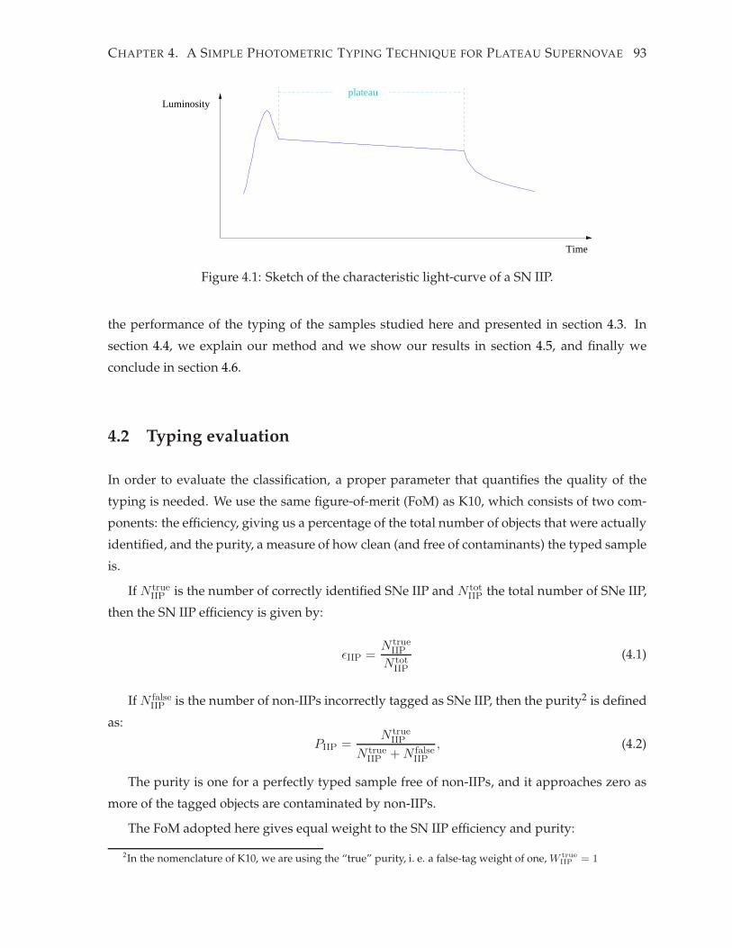
CHAPTER 4. A SIMPLE PHOTOMETRIC TYPING TECHNIQUE FOR PLATEAU SUPERNOVAE 93
Time
Luminosityplateau
Figure 4.1: Sketch of the characteristic light-curve of a SN IIP.
the performance of the typing of the samples studied here and presented in section 4.3. In
section 4.4, we explain our method and we show our results in section 4.5, and finally we
conclude in section 4.6.
4.2 Typing evaluation
In order to evaluate the classification, a proper parameter that quantifies the quality of the
typing is needed. We use the same figure-of-merit (FoM) as K10, which consists of two com-
ponents: the efficiency, giving us a percentage of the total number of objects that were actually
identified, and the purity, a measure of how clean (and free of contaminants) the typed sample
is.
If N trueIIP is the number of correctly identified SNe IIP and N tot
IIP the total number of SNe IIP,
then the SN IIP efficiency is given by:
ǫIIP =N true
IIP
N totIIP
(4.1)
If N falseIIP is the number of non-IIPs incorrectly tagged as SNe IIP, then the purity2 is defined
as:
PIIP =N true
IIP
N trueIIP + N false
IIP
, (4.2)
The purity is one for a perfectly typed sample free of non-IIPs, and it approaches zero as
more of the tagged objects are contaminated by non-IIPs.
The FoM adopted here gives equal weight to the SN IIP efficiency and purity:
2In the nomenclature of K10, we are using the “true” purity, i. e. a false-tag weight of one, W trueIIP = 1

CHAPTER 4. A SIMPLE PHOTOMETRIC TYPING TECHNIQUE FOR PLATEAU SUPERNOVAE 94
FoMIIP = ǫIIP × PIIP
=1
N totIIP
(
N trueIIP
)2
N trueIIP + N false
IIP
(4.3)
The FoM ranges between 0 and 1 and gives a measure of the quality of the typing. We
try to optimize this number in this study, but it is easy to conceive different surveys adopting
alternative FoMs depending on their scientific goals.
4.3 Samples
To study the performance of our SN IIP classification technique, we analyze several real and
simulated datasets. Table 4.1 summarizes these samples.
Table 4.1: SN samples (real and simulations) used to investigate the simple SN IIP typingtechnique. Numbers in parenthesis are for the sets with host-z information, when available
SN sample NIIP Nnon−IIP Redshift∗ Source
Low-z 38 336 z < 0.1 see Table 4.2
SDSS 34 95 0 < z < 0.2D’Andrea et al. (2010);Holtzman et al. (2008)
SNLS 13 381 0 < z < 1.1 –
DES-training (host) 236(218) 1043(1038) 0 < z < 0.6 K10
DES-training/post-mortem (host) 436(492) 738(773) 0 < z < 1.1 See § 4.4.6
DES-challenge (host) 8637(8643) 9710 (9678) 0 < z < 1.1 K10
LSST-training† 233 539 0 < z < 0.7 K10
LSST-training/post-mortem 449 304 0 < z < 1.1 See § 4.4.6
LSST-challenge 26252 16523 0 < z < 1.1 K10
*The redshift range covered by SNe IIP.†The LSST simulated survey has host photo-z for all SNe.
The nearby sample (z < 0.1) is collected from the literature and contains 38 SNe IIP and
336 non-IIP, the vast majority being SNe Ia (see Table 4.2). We also use the first year SDSS-II
sample of 34 SNe IIP (D’Andrea et al. 2010) and 95 SNe Ia (Holtzman et al. 2008). The three
year SNLS sample consists of 13 SNe IIP and 381 non-IIP. These datasets are heavily biased
towards SNe Ia and they do not represent a natural distribution of the different SN types. It is
therefore important to use simulated samples that contain a a more physical mix of SN types.
We use the synthetic DES sample of K10 designed for the classification challenge. This
constitutes a set of ∼ 20000 simulated SNe in the 0.0 < z < 1.1 range, with a spectroscopic

CHAPTER 4. A SIMPLE PHOTOMETRIC TYPING TECHNIQUE FOR PLATEAU SUPERNOVAE 95
training sub-sample of ∼ 1200 SNe. A similar sample with host redshift information is pro-
vided. We investigate both of these samples and show the results for the training sample and
the full sample based on the provided training sample, and also on a deeper training sample
selected here after the challenge was completed (“post-mortem”, see section 4.4.6). The latter
training sample covers a larger redshift range that is more representative of the full sample.
Furthermore, we analyze the artificial LSST sample provided by K103. This is the “deep”
part of their simulations and consists of ∼ 26000 objects with redshifts 0.0 < z < 1.1, and
a spectroscopic training sample of ∼ 700 SNe. The sample also has simulated photometric
redshifts from the host galaxies. Similar to the DES, we perform an additional classification
with an improved training sample after completion of the challenge.
The performance of our method varies considerably between SN samples. This is not sur-
prising given the wide range in sample properties such as the bandpasses, the photometric
quality (signal-to-noise) and cadence of the light-curve coverage. For some low-z SNe, the
light-curve has large gaps without any data, preventing the correct estimation of the start of
the plateau, or the plateau fit itself. For very high-z SNe from the simulated surveys, the
signal-to-noise can be quite low and the typing becomes more unreliable.
We do not attempt to photometrically type all objects from each sample, but instead apply
data selection criterion cuts to remove bad data and optimze the purity. However, note that
N totIIP in our efficiency calculation (Eq. 4.1) reflects the total number of SNe IIP in the sample,
irrespective of these cuts, so the FoM is properly penalized for choosing overly severe cuts. In
all cases we do not make use of the noisy (S/N < 3) blue data of the SDSS (u2.5m and g2.5m),
and of the simulated DES (DESg) and LSST (LSSTu and LSSTg). These surveys have in
some cases extremely unreliable noisy light-curves in these bands.
Table 4.2: Nearby supernovae used in this study
Objects Type Source
SN1968L SN IIP Wood & Andrews (1974)SN1970G SN IIP Winzer (1974); Barbon et al. (1973)SN1973R SN IIP Ciatti & Rosino (1977)SN1986I SN IIP Pennypacker et al. (1989)SN1988A SN IIP Benetti et al. (1991); Turatto et al. (1993)
SN1988H,SN1989C SN IIP Turatto et al. (1993)SN1990E SN IIP Schmidt et al. (1993); Benetti et al. (1994)SN1990K SN IIP Cappellaro et al. (1995)SN1991G SN IIP Blanton et al. (1995)SN1992am SN IIP Schmidt et al. (1994b)SN1992ba SN IIP Pastorello (2003)SN1992H SN IIP Clocchiatti et al. (1996)
SN1994N,SN199eu,SN2001dc SN IIP Pastorello et al. (2004)
3All these sets can be found at http://sdssdp62.fnal.gov/sdsssn/SIMGEN_PUBLIC

CHAPTER 4. A SIMPLE PHOTOMETRIC TYPING TECHNIQUE FOR PLATEAU SUPERNOVAE 96
Table 4.2 – Continued
Objects Type Source
4 SNe SN IIP Pastorello (2003)SN1997D SN IIP Benetti et al. (2001)SN1998A SN IIP Pastorello et al. (2005)SN1999br SN IIP Pastorello et al. (2004)SN1999em SN IIP Hamuy et al. (2001); Leonard et al. (2002b);
Elmhamdi et al. (2003)SN1999gi SN IIP Leonard et al. (2002a)SN2000cb SN IIP Kleiser et al. (2011)SN2001X SN IIP Tsvetkov (2006a)SN2002hh SN IIP Pozzo et al. (2006); Tsvetkov et al. (2007)SN2003gd SN IIP Hendry et al. (2005)SN2003hn SN IIP Krisciunas et al. (2009a)SN2004A SN IIP Hendry et al. (2006); Tsvetkov (2008)SN2004dj SN IIP Chugai et al. (2005); Vinko et al. (2006); Zhang et al.
(2006); Tsvetkov et al. (2008)SN2004ek SN IIP Tsvetkov (2008)SN2004et SN IIP Misra et al. (2007); Sahu et al. (2006)SN2005ay SN IIP Tsvetkov et al. (2006)SN2005cs SN IIP Tsvetkov et al. (2006); Brown et al. (2007); Dessart
et al. (2008); Pastorello et al. (2009b)SN2006bp SN IIP Dessart et al. (2008)SN2008bk SN IIP Van Dyk et al. (2010)SN2008gz SN IIP Roy et al. (2011)SN2009md SN IIP Fraser et al. (2010)SN1990S SN IIn Hamuy et al. (1993)SN1993G SN IIL Tsvetkov (1994)SN1994Y SN IIn Ho et al. (2001)SN1995G SN IIn Pastorello (2003)SN1997bs SN IIn?impostor? Van Dyk et al. (2000)SN1998bw SN Ic McKenzie & Schaefer (1999); Sollerman et al. (2000);
Patat et al. (2001)SN1998S SN IIL Liu et al. (2000)SN1999el SN IIn Di Carlo et al. (2002)SN1999ga SN IIL Pastorello et al. (2009a)
SN2000er,SN2002ao SN Ibn Pastorello et al. (2008b)SN2001B SN Ib Tsvetkov (2006a)SN2002ap SN Ic Gal-Yam et al. (2002a);Yoshii et al. (2003); Foley et al.
(2003)SN2003bg SN IIb Hamuy et al. (2009)SN2002bj SN IIn?.Ia? Poznanski et al. (2010)SN2003jd SN Ic Valenti et al. (2008)SN2003lw SN Ic Malesani et al. (2004)SN2004aw SN Ic Taubenberger et al. (2006)
SN2004A,SN2004gk SN Ibc Elmhamdi et al. (2010)SN2005bf SN Ib Folatelli et al. (2006)SN2005la SN IIb Pastorello et al. (2008a)SN2006aj SN Ic Sollerman et al. (2006); Pian et al. (2006)SN2006gi SN Ib Elmhamdi et al. (2010)SN2006gy SN IIn Agnoletto et al. (2009)SN2006jc SN Ibn Pastorello et al. (2007a, 2008b); Anupama et al.
(2009)SN2007bg SN Ic Young et al. (2010)SN2007bi SN Ic?PI? Young et al. (2010); Gal-Yam et al. (2009)SN2007gr SN Ic Hunter et al. (2009)SN2007rt SN IIn Trundle et al. (2009)

CHAPTER 4. A SIMPLE PHOTOMETRIC TYPING TECHNIQUE FOR PLATEAU SUPERNOVAE 97
Table 4.2 – Continued
Objects Type Source
SN2008es SN IIL Miller et al. (2009)SN2008am SN IIn Chatzopoulos et al. (2011)SN2008ax SN IIb Pastorello et al. (2008c); Roming et al. (2009);
Tsvetkov et al. (2009)SN2008D SN Ib Modjaz et al. (2009)SN2008S SN IIn?impostor? Smith et al. (2009)SN2008iy SN IIn Miller et al. (2010)SN2009bb SNIc Pignata et al. (2011)SN2009jf SN Ib Sahu et al. (2011)SN2010ah SN Ic Corsi et al. (2011)SN2010jl SN IIn Stoll et al. (2010)SN2010gx SN Ic? Pastorello et al. (2010)SN2010X SN Ic?.Ia? Kasliwal et al. (2010)
SN1980N,SN1981d SN Ia Hamuy et al. (1991)SN1981B SN Ia Buta & Turner (1983); Barbon et al. (1982)SN1986G SN Ia Phillips et al. (1987)29 SNe SN Ia Hamuy et al. (1996b)
SN1990N,SN1991T SN Ia Lira et al. (1998)SN1991bg SN Ia Turatto et al. (1996); Filippenko et al. (1992b)
SN1991M,SN1991T, SN Ia Ford et al. (1993)18 SNe SN Ia Altavilla et al. (2004)21 SNe SN Ia Riess et al. (1999a)
SN1994D SN Ia Richmond et al. (1995); Meikle et al. (1996)SN1995D SN Ia Sadakane et al. (1996); Riess et al. (1999a)44 SNe SN Ia Jha et al. (2006)
SN1997cn SN Ia Turatto et al. (1998)SN1998aq SN Ia Riess et al. (2005)SN19998bu SN Ia Suntzeff et al. (1999)
SN1999aa,SN1999cp SN Ia Krisciunas et al. (2000)8 SNe SN Ia Kowalski et al. (2008)
SN1999aw SN Ia Strolger et al. (2002)SN1999by SN Ia Garnavich et al. (2004)
SN1999cc,SN1999cl,SN2000cf SN Ia Krisciunas et al. (2004c)5 SNe SN Ia Krisciunas et al. (2001)
SN1999ee SN Ia Stritzinger et al. (2002); Krisciunas et al. (2004a)SN2000bh,SN2000ca,SN2001ba SN Ia Krisciunas et al. (2004a)
SN2000cx SN Ia Li et al. (2001b)SN2000E SN Ia Valentini et al. (2003); Tsvetkov (2006a)185 SNe SN Ia Hicken et al. (2009)7 SNe SN Ia Krisciunas et al. (2004b)
SN2001el SN Ia Krisciunas et al. (2003)SN2002bf SN Ia Leonard et al. (2005)SN2002cx SN Ia Phillips et al. (2007)SN2002dj SN Ia Pignata et al. (2008)SN2002dr SN Ia Pignata et al. (2004)SN2003cg SN Ia Elias-Rosa et al. (2006)SN2003du SN Ia Anupama et al. (2005); Stanishev et al. (2007)SN2003hx SN Ia Misra et al. (2008)SN2003gs SN Ia Krisciunas et al. (2009b)35 SNe SN Ia Contreras et al. (2010)
SN2004eo SN Ia Pastorello et al. (2007b)SN2004fu SN Ia Tsvetkov (2006b)SN2004S SN Ia Krisciunas et al. (2007)SN2005am SN Ia Li et al. (2006a)SN2005bl SN Ia Taubenberger et al. (2008)

CHAPTER 4. A SIMPLE PHOTOMETRIC TYPING TECHNIQUE FOR PLATEAU SUPERNOVAE 98
Table 4.2 – Continued
Objects Type Source
SN2005cf SN Ia Wang et al. (2009b)SN2005hk SN Ia Phillips et al. (2007)SN2006gz SN Ia Hicken et al. (2007)SN2007qd SN Ia McClelland et al. (2010)
4.4 Method
The characteristic plateau of SNe IIP stands out as an excellent feature for an easy identification
based solely on photometry. Although seemingly straightforward, one needs good sampling
of the light-curve and an automated method that can easily and securely type a large number
of candidates. We use a simple linear fit (in magnitudes) to multi-band photometry and then
use the distributions of the different fit parameters to assign continuous probabilities of being
a SN IIP.
4.4.1 Maximum epoch
First, in order to do a proper linear fit to find a plateau, we need an estimate of the begin-
ning epoch of the plateau. Such a phase happens right after maximum brightness or, in some
cases, a couple of days after maximum. As a first approach we will use the time of maximum
brightness.
The latter is estimated in two steps. First, we get the date of the brightest data point in each
band. We make sure that the signal-to-noise ratio of the selected data points is high enough
(S/N > 5). This signal-to-noise condition is particularly important for the noisy, bluer bands
of the SDSS and simulated DES/LSST samples. The closest estimate of maximum SN light is
given by the first (earliest) of the maxima in the different bands.
This method evidently requires good sampling and pre-maximum data to ensure proper
maximum estimation, although an offset of some days will not affect the post-maximum fit.
The low-z dataset is most affected by this simple technique due to a lack of pre-maximum data
and of dense time sampling. Requiring at least one pre-maximum data point in the light-curve
ensures a better maximum estimate, as will be shown later. In general however, this simple
method is good enough to estimate a first-order maximum for most transients in the different
samples considered.

CHAPTER 4. A SIMPLE PHOTOMETRIC TYPING TECHNIQUE FOR PLATEAU SUPERNOVAE 99
4.4.2 Simple linear post-maximum fit
We now proceed to fit all data past maximum in each band up to a final date, τf , to a line in
magnitudes, or simple power of 10 in flux units4:
f = α10mτ (4.4)
The fit slopes, m, differ among SN types, particularly between SNe IIP (see Figure 4.2) and
other SNe (see Figure 4.3). SNe IIP are expected to have the shallowest negative slopes, or
even positive slopes in some cases, whereas Type I SNe generally should decline very steeply.
Other SNe II types may have a small plateau but of a shorter duration than SNe IIP.
For this to work, the range of the fit is extremely important. If we fit a line to data past
the declining region, where the fluxes are close to zero, we might incorrectly obtain a shallow
slope. Thus, in general, the fits of bluer bands will extend only to a small portion of the post-
maximum light-curve (∼ 20 − 30 days) whereas longer wavelengths fits will cover a longer
span (& 40 − 60 days). The exact final fit epoch for each band depends on the survey and is
studied in § 4.4.4.
Besides the linear fit parameters of Equation 4.4, we add another parameter: the interpo-
lated flux at the end of the fitted region in each band (normalized to maximum flux). This
gives an additional constraint that the shallow linear behavior found by the fit actually corre-
sponds to a plateau and not to the late radioactive decay, where the relative fluxes are much
lower.
These linear fits are not meant to represent a good model to the data; they are just a simple
way to classify the objects. As such, the quality of the fit is irrelevant andwe are only interested
in the parameter space obtained, as shown in next section.
4.4.3 Multi-band fit parameters and probability distributions
The range spanned by the fit slopes in the different bands is the primary tool to differentiate
SNe. As can be seen in Figure 4.4(a) for example, SNe IIP have shallower slopes than other
SN types for the R-band of the nearby sample. SNe Ia clearly decline fastest, followed by
SNe Ibc and other SNe II. SNe IIn have the closest slopes to SNe IIP and are the major source
of contamination.
The distributions of the fluxes at the end of the fitted region relative to maximum are an-
other useful discriminator. Figure 4.5(a) shows the interpolated fluxes at the end of the fitted
region, day 40 after r-band maximum in this case, for the spectroscopic SNLS sample. These
4The measured flux slopes are in (dex × time) but can be converted to (mag × time) multiplying by 2.5

CHAPTER 4. A SIMPLE PHOTOMETRIC TYPING TECHNIQUE FOR PLATEAU SUPERNOVAE 100
5.155 5.160 5.165 5.170Observed Day (x104)
0.2
0.4
0.6
0.8
1.0
1.2
Flu
x (a
rbitr
ary
units
)
-10 0 10 20 30 40 50 60 70 100 150Day since Max
SNIIP: sn1999giz=0.001
UBVRI
(a) SN IIP: SN1999gi
5.398 5.400 5.402 5.404 5.406 5.408Observed Day (x104)
0.0
0.2
0.4
0.6
0.8
1.0
1.2
1.4
Flu
x (a
rbitr
ary
units
)
-50 -40 -30 -20 -10 0 10 20 30 40 50 60Day since Max
SNIIP: sn2006iwz=0.030
u_2.5mg_2.5mr_2.5mi_2.5m
z_2.5m
(b) SN IIP: SN2006iw (SDSS)
5.320 5.325 5.330 5.335Observed Day (x104)
0.0
0.2
0.4
0.6
0.8
1.0
1.2
Flu
x (a
rbitr
ary
units
)
-60 -50 -40 -30 -20 -10 0 10 20 30 40 50 60 70 100Day since Max
SNII-P: 04D4fuz=0.133
gsrsis
zs
(c) SN IIP: 04D4fu (SNLS)
4.945 4.950 4.955Observed Day (x104)
0.0
0.5
1.0
1.5
Flu
x (a
rbitr
ary
units
)
-40 -30 -20 -10 0 10 20 30 40 50 60 70 100Day since Max
SNIIP: LSSTDEEP_SN016130z=0.308
LSSTuLSSTgLSSTrLSSTi
LSSTz
(d) SN IIP: SN016130 (LSST)
Figure 4.2: Examples of linear fits (like Eq. 4.4) to the post-maximum region in multiple bandsof SN IIP light-curves from the low-s, SDSS-II, SNLS and simulated LSST samples. The coloredpoints represent data in the different bandpasses, and the lines the corresponding fits.

CHAPTER 4. A SIMPLE PHOTOMETRIC TYPING TECHNIQUE FOR PLATEAU SUPERNOVAE 101
5.294 5.296 5.298 5.300 5.302 5.304Observed Day (x104)
0.2
0.4
0.6
0.8
1.0
1.2
1.4
Flu
x (a
rbitr
ary
units
)
-10 0 10 20 30 40 50 60 70 100Day since Max
SNIc: sn2003jdz=0.018
UBVRI
(a) SN Ic: SN2003jd
5.362 5.364 5.366 5.368 5.370 5.372Observed Day (x104)
0.2
0.4
0.6
0.8
1.0
1.2
Flu
x (a
rbitr
ary
units
)
-10 0 10 20 30 40 50 60 70Day since Max
SNIa: SDSS1241z=0.086
u_2.5mg_2.5mr_2.5mi_2.5m
z_2.5m
(b) SN Ia: SDSS1241 (SDSS)
5.280 5.285 5.290 5.295Observed Day (x104)
0.0
0.2
0.4
0.6
0.8
1.0
1.2
1.4
Flu
x (a
rbitr
ary
units
)
-70 -60 -50 -40 -30 -20 -10 0 10 20 30 40 50 60 70Day since Max
SNIIn: 03D4ckz=0.189
gsrsis
zs
(c) SN IIn: 03D4ck (SNLS)
5.622 5.624 5.626 5.628 5.630Observed Day (x104)
0.2
0.4
0.6
0.8
1.0
1.2
Flu
x (a
rbitr
ary
units
)
-10 0 10 20 30 40 50 60 70Day since Max
SNIIL: DES_SN024583z=0.045
DESgDESrDESi
DESz
(d) SN IIL: 024583 (DES)
Figure 4.3: Examples of linear fits (like Eq. 4.4) to the post-maximum region in multiple bandsfor different non-IIP supernovae from the low-z, SDSS-II, SNLS and simulated DES samples.The colored points represent data in the different bandpasses, and the lines the correspondingfits.

CHAPTER 4. A SIMPLE PHOTOMETRIC TYPING TECHNIQUE FOR PLATEAU SUPERNOVAE 102
-0.025 -0.020 -0.015 -0.010 -0.005 0.000R-slope
0
10
20
30
40
N
IIPIa
Ibcothers
(a) R-slope
-0.025 -0.020 -0.015 -0.010 -0.005 0.000R-slope
0.0
0.2
0.4
0.6
0.8
1.0
Pro
babi
lity
dist
ribut
ion
IIPIaIbcothers
(b) R-slope distributions
-0.03 -0.02 -0.01 0.00 0.01R-slope
0.0
0.2
0.4
0.6
0.8
1.0
IIP p
roba
bilit
y
IIPIaIbcothers
(c) R-slope SN IIP probabilities
Figure 4.4: (a) Fitted R-slope for different SN types of the low-z sample, (b) correspondingprobability distributions per SN type normalized to peak, and (c) respective SN IIP probabili-ties, pIIP, for each SN based on the IIP probability distribution of (b).

CHAPTER 4. A SIMPLE PHOTOMETRIC TYPING TECHNIQUE FOR PLATEAU SUPERNOVAE 103
0.0 0.2 0.4 0.6 0.8rs-interp
0
10
20
30
N
IIPIa
Ibcothers
(a) rs-flux
0.0 0.2 0.4 0.6 0.8rs-interp
0.0
0.2
0.4
0.6
0.8
1.0
Pro
babi
lity
dist
ribut
ion
IIPIaIbcothers
(b) rs-flux distributions
-0.2 0.0 0.2 0.4 0.6 0.8 1.0rs-interp
0.0
0.2
0.4
0.6
0.8
1.0
IIP p
roba
bilit
y
IIPIaIbcothers
(c) rs-flux SN IIP probabilities
Figure 4.5: (a) Interpolated rs-flux at end of fitted region for different SN types of the SNLSspectroscopic sample, (b) corresponding probability distributions per SN type normalized topeak, and (c) respective SN IIP probabilities, pIIP, for each SN based on the IIP probabilitydistribution of (b).

CHAPTER 4. A SIMPLE PHOTOMETRIC TYPING TECHNIQUE FOR PLATEAU SUPERNOVAE 104
-0.05 -0.04 -0.03 -0.02 -0.01DESg-slope
-0.03
-0.02
-0.01
0.00
DE
Sr-
slop
e
IIPIaIbcothers
(a) r-slope vs g-slope
-0.05 -0.04 -0.03 -0.02 -0.01DESg-slope
-0.03
-0.02
-0.01
0.00
DE
Sr-
slop
e
IIPIaIbcothers
(b) r-slope vs g-slope contours
(c) r-slope vs g-slope SN IIP probabilities
Figure 4.6: (a) Fitted r-slope vs g-slope for different SN types of the simulated DES train-ing sample, (b) corresponding contours of probability distribution per SN type normalizedto peak, and (c) respective SN IIP probabilities, pIIP, for each SN based on the IIP probablitydistribution of (b).

CHAPTER 4. A SIMPLE PHOTOMETRIC TYPING TECHNIQUE FOR PLATEAU SUPERNOVAE 105
-0.020 -0.015 -0.010 -0.005 0.000 0.005LSSTz-slope
-0.2
0.0
0.2
0.4
0.6
0.8
1.0
1.2
LSS
Tz-
inte
rp
IIPIaIbcothers
(a) z-flux vs z-slope
-0.020 -0.015 -0.010 -0.005 0.000 0.005LSSTz-slope
-0.2
0.0
0.2
0.4
0.6
0.8
1.0
1.2
LSS
Tz-
inte
rp
IIPIaIbcothers
(b) z-flux vs z-slope contours
(c) z-flux vs z-slope SN IIP probabilities
Figure 4.7: (a) z-flux, interpolated at the end of the fit region, vs fitted z-slope for the differentSN types of the simulated LSST training sample, (b) corresponding contours of probabilitydistributions per SN type, and (c) respective SN IIP probabilities, pIIP, for each SN based onthe IIP probability distribution of (b)

CHAPTER 4. A SIMPLE PHOTOMETRIC TYPING TECHNIQUE FOR PLATEAU SUPERNOVAE 106
are higher for SNe IIP, for which the hydrogen envelope is still powering the optical display.
Together with a flat plateau slope, these two parameters can differentiate SNe IIP and ensure
that a shallow slope is not due to the earlier radioactive decline at the end of the light-curve of
some SNe.
Evenmore enlightening is the use of multi-band slope-slope and slope-flux spaces to select
SNe IIP. Parameter spaces of different band combinations take advantage of the distinguish-
ing color evolution of various SNe. Figures 4.6(a) and 4.7(a) show that SNe IIP in the simu-
lated DES and LSST training samples stand out from other SNe in particular regions of high
slopes and large post-maximum fluxes. Multiple parameter spaces like these can discriminate
SNe IIP, although overlapping objects still exist.
The SN classification could be based on the visual determination of particular SN IIP
regions in the different parameter spaces. This, however, would be a difficult and time-
consuming human component that does not ensure the most successful classification. With
many parameter spaces and a lot of overlapping SNe from different types, we instead assign
to each SN a continuous probability of being of each SN type. In order to do this, we use 1D
and 2D kernel density estimators for our training set divided in SN types for each parameter
space under consideration. The kernel density estimators provide probability distributions,
from which a probability for each object is drawn. Figures 4.4(b) and 4.5(b) show the resulting
1D probability distributions, normalized to maximum, for the previous R-band slope of the
low-z set and for the r-band flux of the SNLS. It is obvious from this procedure that a better
typing will be achieved with a more complete training sample that contains enough SNe of
multiple types (see $ 4.4.6). For the 2D cases, Figures 4.6(b) and 4.7(b) show the contours of
the probability distributions of slope-slope and slope-flux spaces for the training samples of
the DES and LSST, which represent a better suited database to study photometric typing.
Each SN is then assigned a “IIP probability” per parameter space (a value between 0 and 1)
by interpolating the probablity distribution with the SN parameters. Figures 4.4(c) and 4.5(c)
show an example of the obtained IIP probabilities for the 1D distributions shown earlier, and
Figures 4.6(c) and 4.7(c) for the 2D spaces. Similarly, we calculate for each SN a probability of
being of the other types considered.
In this way, we obtain for each object a probability of being a SN IIP, piIIP, and probabilities
of being other SN types, like piIa, p
iIbc, p
iIIL,IIn, where i denotes each parameter space. All these
probabilities are put together into a single matrix, P, of size m × n, with n the number of SNe
considered and m the number of probabilities. In order to constrain the importance of each of
these probabilities, we want to find a vector of weights, w, of size m for each probability, that
quantifies the importance of each space for the typing. We therefore solve following equation
for w:

CHAPTER 4. A SIMPLE PHOTOMETRIC TYPING TECHNIQUE FOR PLATEAU SUPERNOVAE 107
c = w × P, (4.5)
where c is a vector of n size. For the training set it is filled with 1 for SNe IIP and −1 non-IIP.
The resulting vector of weights w can be then used for any SN to get a final SN IIP probability
cSN via the same equation.
Finally, a SN IIP is tagged if cSN > 0 (see Figure 4.8). This is the standard approach used in
this study. However, one can require a tighter constraint like cSN > 0.5 if an increase in purity
(Eq. 4.2), in detriment of the efficiency (Eq. 4.1), is preferred.
-2 -1 0 1 2PIIP-Pcont
0
5
10
15
20
N
real IIPreal cont
Figure 4.8: Difference of final probabilities of being a SN IIP or a non-IIP for all SNe of theSDSS-II sample. The filled histogram represents real spectroscopic SNe IIP and the greenhistrogram are the contaminants (here SNe Ia). A SN IIP is tagged if PIIP − Pcont > 0.
4.4.4 Variation of fitting conditions
There are several factors in this method that can considerably affect the typing quality. Two
major elements considered in this section are: a) the post-maximum time range allowed in
the fit, represented by the initial τ bi and final τ b
f epochs, for each bandpass filter b; and b) the
amount of data required for the fit. Here, we explore these variables and find the optimal ones
for each survey by maximizing the FoM.

CHAPTER 4. A SIMPLE PHOTOMETRIC TYPING TECHNIQUE FOR PLATEAU SUPERNOVAE 108
Fit duration
For simplicity, we always assume τ bi = 0, i. e. the initial fitting epoch always corresponds to
the epoch of maximum flux. This assumption is expected to be quite accurate except for just a
couple of days in longer wavelength bands, for which the plateau phase might start later. We
investigate different combinations of τ bf , the final fitting epoch, ranging from 20 to 100 days
after maximum. Generally τf also happens later for redder filters. For each combination, we
calculate the FoM (Eq. 4.3) and find the values for which it is optimized. We find that a good
typing is achieved by fitting longer periods for longer wavelengths and shorter periods for
shorter ones, as it is expected due to the SN IIP color evolution. The day ranges used for all
surveys are shown in Table 4.3.
Data requirements
Besides the initial signal-to-noise cull required for the bluer bands of the SDSS, simulated DES
and LSST (see section 4.3), we also investigate different number of data points required in
the fit. Normally a minimum of 2 data points per band is needed to fit a line. However, for
data with long absence of points, like for the low-z sample, the fit might be driven by only
the initial part of the assumed plateau and no posterior data, or vice-versa. We can avoid
misidentifications of SNe IIP by requiring data more evenly sampled in the fit, like at least
one epoch in the first half of the fit range and at least another point in the second half. By
doing this, we might affect the recovery efficiency but we will ensure a purer sample. Several
combinations of data requirements were investigated but we found the best FoM results for
two cases: a) one data point in each, the first and second, half of the fitted region, or b) three
data points in the whole range fitted. The final data requirements per SN sample are also
shown in Table 4.3.
The results for the duration of the fit and the number of data required in the fit were found
by investigating a variety of combinations of these in the different bands. Figure 4.9 shows
how the FoM is affected by the choice of these parameters for a combined low-z, SDSS and
SNLS dataset. Each x-value corresponds to a particular set of combinations, x = 0 is for
example a typing study requiring one data point in each, the first and second half, of a 0 − 20
days fit range in rest-frame for all survey bands. The case x = 14, where the maximum FoM
is found (for no redshift information), corresponds to three data points in three evenly spaced
sections of a 0 − 50 day range in each band. With redshift information, the best FoM occurs
at x = 28, where 2 data points are required in the range of 0 − 20 days for the u2.5m/us- and
g2.5m/gs -bands, and 2 data points in the range 0 − 40 days for r2.5m/rs- and i2.5m/is -bands.

CHAPTER 4. A SIMPLE PHOTOMETRIC TYPING TECHNIQUE FOR PLATEAU SUPERNOVAE 109
0 10 20 30 40different obscull/finalday
0
20
40
60
80
100
FoM
(%
)
z-infono z-info
Figure 4.9: Figure of Merit (FoM) as a function of different combinations of required dataand duration of the fit in the different bands. The solid/dashed lines represent studies for acombined low-z, SDSS and SNLS sample with/without redshift information.

CHAPTER4.A
SIM
PLEPHOTOM
ETRIC
TYPIN
GTECHNIQ
UE
FORPLATEAUSUPERNOVAE110
Table 4.3: Duration and data requirement of fitted region for each SN sample (real and simulated). Numbers in parenthesis are for thesets with spec-z or host-z information, when available
SAMPLE Data⋄ Filter 1 Final day∗ Filter 2 Final day∗ Filter 3 Final day∗ Filter 4 Final day∗ Filter 5 Final day†
Low-z (with zsp) 2h(2h) U 30(25) B 45(40) V 50(50) R 65(60) I 65(60)
SDSS (with zsp) 3t(3t) u2.5m 20(25) g2.5m 25(30) r2.5m 30(35) i2.5m 35(45) z2.5m 35(45)
SNLS (with zsp) 2h(3t) gs 30(20) rs 45(25) is 60(30) zs 65(35) – –
DES (with zhostph ) 2h(3t) DESg 40(40) DESr 50(45) DESi 55(60) DESz 65(65) – –
DES-post-mortem (with zhostph ) 3t(3t) DESg 35(30) DESr 50(45) DESi 60(55) DESz 75(65) – –
LSST (with zhostph ) 1h(1h) LSSTu 20(20) LSSTg 25(30) LSSTr 30(35) LSSTi 45(45) LSSTz 45(45)
LSST-post-mortem (with zhostph ) 3t(3t) LSSTu 40(20) LSSTg 50(25) LSSTr 60(45) LSSTi 70(60) LSSTz 70(60)
⋄The data required is either: a) two data points, one in the first half of the fitted region and another in the second half (“2h”), or b) three data points inthe full fitted region (“3t”)∗The final day after maximum brightness†The day for filter 5 is not separately fitted, but the same day as filter 4 is used.

CHAPTER 4. A SIMPLE PHOTOMETRIC TYPING TECHNIQUE FOR PLATEAU SUPERNOVAE 111
4.4.5 Redshift information
In our fittingmethod, the redshift knowledge allows us to improve the fits by correcting the SN
epochs to rest-frame, so that the right portion of the light-curve is allowed in the fit. Although
the final epochs, τ bf , of the fits are optimized for each survey (see previous section), in samples
with large redshift ranges, the use of the same final epoch across different redshifts will lead to
biases in the fit parameters. A redshift prior, spectroscopic or photometric, should reduce this
effect by correcting all epochs by a (1 + z) factor. We investigate the inclusion of spectroscopic
redshifts for the low-z, SDSS-II, SNLS and host photometric redshifts for the DES and LSST
simulated samples.
0 10 20 30 40 50different obscull/finalday
0
20
40
60
80
100
FoM
(%
)
0.050.150.250.350.450.550.650.750.850.95
Figure 4.10: Figure of Merit (FoM) as a function of different combinations of required data andduration of the fit. The different lines represent studies in different 0.1 redshift bins of the DESsimulated data set with host-z information.
Furthermore, in the case where the light-curves of SNe IIP, or other types, evolve with
redshift due to intrinsic variation, or observational biases, by dividing the training sample into
redshift bins, we can include those effects in the typing technique. This binned typing trains
each z-bin separately and finds independent optimal slope-slope and slope-flux distributions
for each one. Thus, two SNewith the same fit slopes and fluxes but at different redshifts might
have different SN IIP probabilities. For this method to be possible, one needs a good training
sample with enough SNe covering all redshifts. We implement it uniquely for the DES and
LSST simulated samples, where there are enough SNe in each bin.

CHAPTER 4. A SIMPLE PHOTOMETRIC TYPING TECHNIQUE FOR PLATEAU SUPERNOVAE 112
Additionally, when redshift information is available, the search for optimal fitting condi-
tions, like the fit duration and data requirements presented in last section, can be separated for
different redshift bins. The procedure is shown in Figure 4.10 for the simulated DES survey
with host-z information. Each line shows a different 0.1 redshift region up to z = 1.0. One can
see that the FoM is not always optimized for the same combination. The resulting fit durations
differ as a function of redshift, as shown in Figure 4.11. This is partly due to the extension of
the relevant light-curve portions in the observer frame at higher redshift, but also to a different
sampling of the light-curve at different redshifts depending on the survey characteristics.
The typing with redshift information (and binned training) only improves the FoM by a
few percent. The results with no redshift information are remarkably similar (see Table 4.5 and
Figures 4.13 and 4.14).
0.0 0.2 0.4 0.6 0.8 1.0redshift
0
20
40
60
80
Fin
al fi
t day
DESgDESrDESi
DESz
Figure 4.11: Fit range per band for different redshift bins of the simulated DES sample
4.4.6 Training set
In this section we explore the importance of the training setd provided by K10 for the DES and
LSST typing, and provide other ones that are more representative of the full population.
The original spectroscopic training sets of the simulated samples were based on limiting
magnitudes (e. g. 21.5 mag in the DESr-band for a 4m telescope and 23.5 mag in the DESi-
band for a 8m telescope, see K10) that lead to a heavy bias in the spectroscopic redshift distri-
bution compared to the full sample. The SNe IIP of the training sets go only to z ∼ 0.6 − 0.7,

CHAPTER 4. A SIMPLE PHOTOMETRIC TYPING TECHNIQUE FOR PLATEAU SUPERNOVAE 113
while for the entire sample they extend all the way to z ∼ 1.1 (see Table 4.1). More than 50% of
the plateau supernovae are in a regime that is not probed by the training sample. These SNe
have quite different, noisier and less sampled light-curves, which greatly decreases the typing
efficiency at higher-z. Moreover, the ratio of SNe Ia to other SN types is over-represented in
the training sets. All these biases lead to a training set that is not representative of the real
dataset and will affect negatively the performance of the classification. This issue can clearly
be seen in the results of the SN challenge, for which most of the methods presented did much
worse when run on the training sets themselves. Here, we find that the spectroscopic sets
have FoMs of 78% (DES) and 64% (LSST), dropping down to 31% (DES) and 21% (LSST) for
the entire sample (see Table 4.5).
0.0 0.2 0.4 0.6 0.8 1.0spec-z
0.0
0.2
0.4
0.6
0.8
1.0alltrainingpost-mortem
Figure 4.12: Redshift distribution of the entire simulated DES sample normalized to peak (grayshaded), the provided training sample (red diagonal), and the post-mortem training sample(blue empty)
We therefore attempt using a different training subset to classify all SNe. As proposed
by Richards et al. (2011), by increasing the deepness of the survey (e. g. to 23.5 mag for the
DESr-band) and randomly picking up SNe below this limit, higher-z regimes are covered
and a better representation of the sample is achieved (see Figure 4.12 for the DES sample).
We decrease the efficiency parameters for spectroscopic observation (Equation 2 and Table 3
of K10) to have a similar number of spectroscopic objects than the original one, as shown in
Table 4.1. We name the typing of the full sample based on this new training sample, the “post-

CHAPTER 4. A SIMPLE PHOTOMETRIC TYPING TECHNIQUE FOR PLATEAU SUPERNOVAE 114
mortem” DES/LSST samples. The final efficiencies and FoMs are much improved: 63% (DES)
and 58% (LSST) and are shown in Figures 4.13 and 4.14. The purities drop slightly due to a
lower number of contaminant (non-IIP) objects in the post-mortem training sample compared
to the original sample.
4.5 Results
Our final efficiencies, purities and FoMs are summarized in Table 4.4 for all surveys. We note
that these were obtained in order to optimize the FoM, regardless of the separate efficiencies
and purities. Nevertheless, we find that the purities for all real and simulated samples are
higher than ∼ 80%. This shows that this technique is a robust SN IIP photometric typing
independent of the redshift range and applicable for a variety of surveys.
The efficiencies calculated here represent a percentage of the full samples, before light-
curve selection cuts and other culls. For the real datasets, they are normally higher than 80%
but go as low as 70% for the low-z sample due to the scarcely sampled light-curves that do
not pass the data requirements for the fit (see section 4.4.4). On the other hand, the complete
simulated samples have very low efficiencies, lower than 40%, pulling also the FoMs down.
Two important factors affect the efficiency of the simulated samples: a) a training sample
that does not span to high redshifts, and b) very noisy and poorly sampled data, especially
at high redshift, that either is culled out, or that affects the maximum epoch estimate or the
post-maximum fit.
We address the first concern by selecting a different training sample of the same size but
deeper in brightness (see section 4.4.6). The obtained efficiencies increase by 30-40%. We
show the results as a function of redshift for both simulated samples in Figures 4.13 and 4.14.
The full sample trained with the original spectroscopic subset (dashed lines) decrease with
redshift very fast. The post-mortem analysis (solid lines), on the other hand, remain constant
with redshift. We therefore agree with the findings of Newling et al. (2011) and Richards et al.
(2011) that a better training sample, more representative of the full set, is needed for accurate
typing. Similarly to Newling et al. (2011), we find that our technique performs very well
without any redshift information benefiting only a small percentage from the inclusion of a
redshift analysis.
We cannot do much to directly address the second concern of some poor quality light-
curves in the simulated data. However, to quantify the effect of these in the final efficiencies
and FoMs, we can calculate the efficiencies respect to the culled sample instead of the full
sample. By requiring a new “culled sample” consisting of only SNe with enough data points
in the fitted region (as in section 4.4.4), and with high signal-to-noise for the simulated surveys

CHAPTER 4. A SIMPLE PHOTOMETRIC TYPING TECHNIQUE FOR PLATEAU SUPERNOVAE 115
0.0 0.2 0.4 0.6 0.8 1.0Redshift
0
20
40
60
80
100
Dia
gnos
tic (
%)
FoMEfficiencyPurity
0.0 0.2 0.4 0.6 0.8 1.0Redshift
0
20
40
60
80
100
Dia
gnos
tic (
%)
FoMEfficiencyPurity
Figure 4.13: Figure of Merit (FoM) (black squares and lines), efficiency (blue diamonds andlines) and purity (red crosses and lines) as a function of redshift for the DES sample trainedwith the post-mortem setwithout prior redshift information (upper) andwith host photometricredshift information (lower). The dashed line is the FoM for the DES challenge (based on theoriginal training sample) and dotted line for the FoM of just the original DES training set.

CHAPTER 4. A SIMPLE PHOTOMETRIC TYPING TECHNIQUE FOR PLATEAU SUPERNOVAE 116
0.0 0.2 0.4 0.6 0.8 1.0Redshift
0
20
40
60
80
100
Dia
gnos
tic (
%)
FoMEfficiencyPurity
0.0 0.2 0.4 0.6 0.8 1.0Redshift
0
20
40
60
80
100
Dia
gnos
tic (
%)
FoMEfficiencyPurity
Figure 4.14: Figure of Merit (FoM) (black squares and lines), efficiency (blue diamonds andlines) and purity (red crosses and lines) as a function of redshift for the LSST sample trainedwith the post-mortem set, without prior redshift information (upper) and with host photomet-ric redshift information (lower). The dashed line is the FoM for the LSST challenge (based onthe original training sample) and dotted line for the FoM of just the original LSST training set.
CHAPTER 4. A SIMPLE PHOTOMETRIC TYPING TECHNIQUE FOR PLATEAU SUPERNOVAE 117
(S/N > 3), we obtain the results quoted in the last column of Table 4.5. These are clearly higher,
especially for the low-z and simulated samples, for which the efficiencies were particularly
low. By doing this, the decrease in the number of tagged SNe IIP tagged is 8− 25%. To ensure
a better estimate of the day of maximum brightness, we can include the requirement of at least
one pre-maximum data. For the low-z sample, the efficiency increases to 94% in this case,
but the decrease in the number of tagged SNe IIP is much larger than 60%. This shows the
importance of quality data to obtain higher efficiencies.
4.6 Conclusions
The technique presented here, albeit simple, has great power to select SNe IIP across a wide
range of redshifts and surveys. It is based on simple linear fits in magnitudes to multi-band
photometry and the analysis of the fitted parameter spaces. Without the need of redshift
knowledge, it also avoids the cumbersome use of templates and K-corrections, and any evo-
lutionary effects related to them.
The method is quite robust at separating SNe IIP from other SNe with purities higher than
80% for all real and simulated datasets considered. The highest source of misidentification
are SNe IIn, which may also have shallow decline rates after maximum brightness. The SN IIP
efficiencies are higher than 60% for all redshifts as long as proper training samples, representa-
tive of the full sample, are used. They can be further increased with high-quality well-sampled
photometry. Additional redshift information, such as host photo-z, provides an increase in the
FoM of a few percent.
The method introduced here is easily implemented for current and coming transient sur-
veys. As the number of SNemultiply, and the cadence becomes shorter, the technique provides
a fast and secure way of photometrically classify plateau supernovae.

CHAPTER4.A
SIM
PLEPHOTOM
ETRIC
TYPIN
GTECHNIQ
UE
FORPLATEAUSUPERNOVAE118
Table 4.4: Efficiencies, purities and FoMs for each SN sample (real and simulated). Numbers in parenthesis are for the sets with spec-zor host-z information, when available
SAMPLE NIIP N trueIIP Ncont N false
IIP Efficiency Purity FoM Culled-FoM
Low-z (with zsp) 38 35(35) 336 2(1) 0.92(0.92) 0.96(0.97) 0.88(0.89) 0.92(0.93)
SDSS (with zsp) 34 34(34) 95 0(0) 1.00(1.00) 1.00(1.00) 1.0(1.0) 1.0(1.0)
SNLS (with zsp) 12 12(12) 381 0 1.00(1.00) 1.00(1.00) 1.00(1.00) 1.00(1.00)
Low-z+SDSS+SNLS (with zsp) 46 33(33) 629 9(1) 0.91(0.91) 0.79(0.96) 0.72(0.87) 0.79(0.87)
DES-training (with zhostph ) 236(218) 198(201) 1043(1038) 8(15) 0.84(0.92) 0.96(0.93) 0.81(0.85) 0.91(0.92)
DES-challenge (with zhostph ) 8637(8643) 3196(3112) 9678(9710) 655(424) 0.37(0.36) 0.83(0.88) 0.31(0.32) 0.42(0.43)
DES-post-mortem (with zhostph ) 8637(8643) 6737(6828) 9678(9710) 1580(1499) 0.78(0.79) 0.81(0.82) 0.63(0.65) 0.72(0.79)
LSST-training (with zhostph ) 233 166(178) 539 19(21) 0.71(0.76) 0.90(0.90) 0.64(0.68) 0.79(0.79)
LSST-challenge (with zhostph ) 26252 6891(8663) 16523 1513(1528) 0.26(0.33) 0.82(0.85) 0.21(0.28) 0.33(0.35)
LSST-post-mortem (with zhostph ) 26252 19540(19479) 16523 5511(5178) 0.74(0.74) 0.78(0.79) 0.58(0.59) 0.70(0.71)

Chapter 5
Summary and Outlook
The importance of supernovae should not be underestimated. Supernovae are fundamental
for life (youwould not be reading this without them) and they are a key feature in the life cycle
of stars. Themechanisms involved in the explosion are a probe of fundamental physics, where
the four forces of nature play an essential role. The frequency of their occurrence throughout
the history of the universe and the high energy released havemade thema favorite explanation
of unanswered questions in astronomy such as energy input in collapsing molecular clouds
for star formation or AGN feedback. Despite several efforts, pivotal problems in explaining
their nature remain. This thesis contributes to the understanding of these explosive events.
5.1 Type Ia supernovae
Believed to come from low-mass stars that end their lives as exploding white dwarfs in a bi-
nary system, type Ia supernovae have been essential for cosmology for more than a decade.
However, despite several efforts, the nature of the companion star donating mass, and the
physics of the explosion are still a mystery and a source of systematic uncertainty in the deter-
mination of the equation of state of dark energy.
The faintest of SN Ia explosions, “subluminous” objects, are several magnitudes dimmer
than typical SNe Ia; they are very short-lived and have extreme red colors. They have been
hard to include in a common comprehensive progenitor and explosion scenario, and they had
to be left out of cosmological studies, despite contributing to ∼ 18% of the nearby SN Ia rate.
This thesis has addressed some fundamental questions of SNe Ia, particularly subluminous
SNe Ia.
We have searched for subluminous SNe Ia in the SNLS at redshifts higher than z > 0.1,
where they remained previously unobserved. We found a fraction of 18 low-stretch SNe Ia up
to z = 0.6 showing that they constitute a natural continuation of the population even at high
119

CHAPTER 5. SUMMARY AND OUTLOOK 120
redshift. They have similar photometric properties than the local sample and they are also
found in sites of low star formation. The measured rate as a function of redshift is consistent
with a constant or decreasing fraction with redshift, compared to the increasing normal SN Ia
rate. This confirms that the SN Ia population mix evolves with redshift. Subluminous SNe Ia
do not follow the cosmic star formation history (even less than normal SNe Ia) and probably
come from a population of lower mass progenitors (or higher metallicity) than other SNe Ia.
The search for evolution of SN Ia properties is extremely important for cosmological anal-
yses. Numerous studies show that the evolutionary bias is low. We find an interesting popu-
lation of bluer low-stretch SN Ia candidates at z & 0.7. This set has a definite different color
distribution that is abnormal for those light-curve widths, but they are found at the limiting
magnitude of the SNLS. Several attempts were made to discard these objects, as SN Ibc con-
taminants, or through larger photometric uncertainties, but their origin remains unknown. If
their properties turn out to be real, they could either represent a new class of transients with
faint and fast-evolving light-curves and passive hosts, or they are a yet unknown potential
evolutionary state of SNe Ia.
This thesis also presented the rise-time study of a large variety of SN Ia light-curves, par-
ticularly the subluminous SNe Ia previously found. Using the well-sampled data of the SNLS
but also the published data of the SDSS and some other nearby SNe Ia, we K-corrected all
data points to rest-frame B-band and overlaid them all together to study the rise-time behav-
ior. By grouping the SNe Ia by stretch, we investigate possible differences in the early portion
of the light-curve. We find that all SNe Ia, from low- to high-stretch, including subluminous
ones, when stretch-corrected, are well represented by a quadratic rise to maximum brightness
lasting approximately 17.00 days for the template we use. At a 1σ level, the wide variety of
SN Ia explosions all agree with this behavior.
Different rise-times among SN Ia populations would have important consequences that
could hint towards additional parameters shaping the explosions, particularly in the outer
layers (e. g. Hoflich et al. 2010; Fink et al. 2010). Although we observe a possible trend of
longer rise-times for lower stretch objects, after stretch-correction, the different samples are
consistent within the errors. We find no need for a separate independent component to model
the early rise of the light-curve. To the level reached by the data, secondary parameterizations
besides stretch do not significantly improve the light-curve modeling, not even a two-stretch
parameterization as found in other studies. This shows once again that SNe Ia are an extremely
homogenous sample throughout the entire light-curve. This is remarkable considering the
ample range of luminosities and colors covered by all SNe Ia. It argues for a common explosion
mechanism and keeps cosmologists tranquil.
Lastly, I would like to point out an important evolution in the SN Ia paradigm since the

CHAPTER 5. SUMMARY AND OUTLOOK 121
start of this thesis. For many years, the scientific community recognized the value of the dou-
ble degenerate scenario, but it was often overshadowedby the single degeneratemechanism to
SNe Ia with arguments of theoretical robustness. It was seen as unlikely to drive a thermonu-
clear runaway via the merger of two WDs. Nowadays, there still are theoretical drawbacks
for the DD scenario, although advances are being made, but the viewpoint is shifting thanks
to the multiple observational evidences that argue against the SD path as the main source for
SNe Ia.
The consistent lack of hydrogen in the spectra, the missing observed X-ray emission from
their accreting progenitor systems, the confirmed existence of a number of super-Chandrasekhar
explosions, the lack of signature of companions in the early portion of the light-curves, and the
discrepant delay-time distributions inferred from the SN Ia (and SN Ia remnant) rate evolution
in different environments, strongly question the SD viability for most SNe Ia.
The need for another channel propels the DD scenario. Despite its theoretical counterargu-
ments, this mechanism is in harmony with most of the mentioned observations. It would also
naturally explain the relation between environments and SN Ia properties: brighter and more
energetic SNe Ia would come from more massive progenitors, more common in star-forming
regions while fainter and less energetic SNe Ia are the result of less massive progenitors hap-
pening in more evolved passive environments. Furthermore, recent theoretical studies have
revived the possibility of sub-Chandrasekhar explosions. The fraction of WD mergers whose
total mass is below the Chandrasekhar limit can easily explain the total rate of SNe Ia, the only
empirical evidence missed by the regular DD scenario.
This picture of SN Ia progenitors is especially suited for subluminous SNe Ia. As this work
has shown, their early-type environments all the way to high redshift and the DTD fits to
their rate strongly suggest a low mass origin. Being ten times fainter and with very low 56Ni
masses synthesized, they are hard to reconcile with Chandrasekhar mass explosions. As a
matter of fact, successful subluminous explosions have been produced via sub-Chandrasekhar
deflagrations or through WD mergers. From the subluminous SN Ia perspective, there is no
better progenitor scenario than themerger of twoWDs in a binary of low total mass producing
a weak sub-Chandrasekhar explosion (although the predicted fraction might be low, seeMeng
et al. 2011).
If SNe Ia have so similar light-curves (after stretch-correcting) and spectra suggesting a real
common origin, and subluminous are the extreme end of the population (Doull & Baron 2011),
it is quite tempting to sustain that their progenitors are the lowest mass end of a continuous
WDmass distribution that could extend all theway to the progenitors of super-Chandrasekhar
SNe Ia at the other end. Admittedly, common explosion physics producing such a huge range
of output properties have been difficult to model and require an incredible effort that only

CHAPTER 5. SUMMARY AND OUTLOOK 122
recent and future simulating techniques and computational powerwill be able to solve. On the
other hand, recurring to different progenitors scenarios for such homogeneous events seems
increasingly improbable.
The next years of SN Ia science will certainly continue to see a rapid evolution in our
understanding of the underlying physics. New surveys at low and high redshift open up
exciting possibilities to soon reveal their true nature. The Palomar Transient Factory (PTF;
Law et al. 2009; Rau et al. 2009) for instance can study the nature of subluminous SNe Ia in
more detail and even find fainter and/or rare unseen objects (Sullivan et al. 2011b) that could
provide the missing pieces of the SN Ia puzzle. Comprehensive surveys like the Catalina Real-
Time Transient Survey (CRTS; Drake et al. 2009), CHASE (Pignata et al. 2009), Pan-STARRS
(Tonry & Pan-STARRS Team 2005) and future Dark Energy Survey (DES; Bernstein et al. 2009),
Skymapper (Schmidt et al. 2005) and the Large Synoptic Survey (LSST; Ivezic et al. 2008) will
study SN Ia environments across different redshifts and their rate evolution for increasingly
accurate determinations of the delay-times. Better cadence since the early times after explosion
will further constrain progenitor radii from the interaction in the ejecta seen in the light-curve
rise portion, possibly ruling out main-sequence companions as has been done for red giant
companions. Finally, the future improvement of SN Ia science will contribute to precision
cosmology with better-understood systematics (besides the increase in the number of objects
studied). The elusive nature of the dark energy may be apprehended once we also nail the
nature of SNe Ia.
5.2 Plateau supernovae
Plateau supernovae are the most common of all supernovae. They are core-collapse SNe from
progenitors of initial masses between 8 − 17M⊙. Their optical light-curve is easily recogniz-
able with a characteristic plateau after maximum brightness. The study of core-collapse su-
pernovae is in a more infant state than SNe Ia. The prioritization of SNe Ia for cosmology
and the –in principle– better understood progenitors and explosions of CC SNe has left them
somewhat straggled. Nevertheless, due to their high rate and the rolling technologies of cur-
rent (and coming) surveys, many unanalyzed SN IIP light-curves are stored in the databases.
Quality photometry allows very interesting scientific studies but we need proper classification
algorithms, hopefully automated for the huge coming transient searches.
In this thesis, we have introduced a simple and effective photometric typing technique for
SNe IIP. It uses linear magnitude fits to multi-band post-maximum data and post-maximum
fluxes to find appropriate regions of high SN IIP probability to select candidates. We tested the
technique with current low-z and high-z data, and with simulated coming surveys. We find

CHAPTER 5. SUMMARY AND OUTLOOK 123
the method to be very accurate at discriminating SNe IIP; the tagged samples are always more
than 80% pure. The fraction of SNe IIP typed respect to the entire set varies a lot depending
on the survey. We find that these IIP efficiencies can be improved with better spectroscopic
training samples that are more characteristic of the entire samples. Good data, evenly sam-
pled across all epochs, particularly prior to maximum and during the plateau phase ensures a
higher fraction of selected SNe IIP.
Preliminary studies of our sIImP method employed on the SNLS database reveal a photo-
metric SN IIP dataset of ∼ 350 objects with host photo-z’s up to z ∼ 0.7. This exceeds by far
the number of published plateau supernovae and reaches unprecedented redshifts. Multiple
interesting scientific studies can be performed with this dataset.
A first interesting analysis is a measurement of the SNLS IIP rate as a function of redshift.
Previous measurements at high-z grouped all core-collapse SNe together (Dahlen et al. 2004;
Bazin et al. 2009; Graur et al. 2011), which involves interesting research topics like an observed
missing fraction (compared to the massive star formation rate) due possibly to obscuration or
weak SNe (Horiuchi et al. 2011). Measuring the SN IIP rate individually, however, has also
a very important scientific value. Being directly related to the star formation history of the
universe, the normalization of the rate would give us the IMF fraction of massive stars that
lead to such explosions, providing thereby a direct measure of the progenitor mass range.
With the current non-detection of progenitors with MZAMS > 17M⊙, an independent upper
mass limit would test these results. This study is a natural high-priority follow-up that will
benefit from the tools developed for the SN Ia rate measurement.
Considerable effort has been dedicated to characterize and understand the light-curves of
SNe IIP, particularly the plateau phase (e. g. Nadyozhin 2003) but also the early times (Cowen
et al. 2010). Theoretical and hydrodynamical models try to relate SN physics such as explo-
sion energy, 56Ni mass produced, progenitor mass and radius, with observational properties
like plateau duration and luminosity, and expansion velocities (e. .g Tominaga et al. 2009;
Utrobin & Chugai 2009; Dessart & Hillier 2011; Bersten et al. 2011). This led to the recogni-
tion of SNe IIP as distance indicators, potentially even in the UV (Gal-Yam et al. 2008). Kasen
& Woosley (2009) have even suggested a 20% accuracy in distance estimation based solely
on photometric SN IIP parameters. The large photometric dataset of the SNLS opens up the
opportunity to study a variety of aspects of SN IIP light-curves, their relation to physics and
their standardization capabilities. This dataset is the exact high-z counterpart to nearby SN IIP
studies (e. g. Poznanski et al. 2009; D’Andrea et al. 2010) that is needed to understand possible
evolution and their viability as cosmological rulers. Again, we will benefit from the develop-
ments in the study of the rise-time of SN Ia light-curves.
If SNe Ia have turned to be one of the favorite transients studied by astronomers in the

CHAPTER 5. SUMMARY AND OUTLOOK 124
past decades, type IIP and other core-collapse supernovae are on the way of becoming as, or
even more exciting. Large numbers will be discovered by future surveys, even if it is as a side
product of large SN Ia searches. With reliable typing techniques and good quality data, we
might be able to fully understand the final stages of massive stars, how they explode, when
they occur and if they always have an optical display.
Plateau supernovae might become a new robust independent cosmological probe. With
their better-understood progenitors and atmosphere physics, as well as their abundance (par-
ticularly at higher redshift where the cosmic star formation increases), they will offer a unique
cosmological tool for future surveys such as the aforementioned LSST, the proposed Joint Dark
Energy Mission (JDEM), the James Webb Space Telescope (JWST) and future large-class tele-
scopes.

Bibliography
Agnoletto, I. et al. 2009, ApJ, 691, 1348
Aguirre, A. 1999, ApJ, 525, 583
Aldering, G., Knop, R., & Nugent, P. 2000, AJ, 119, 2110
Aldering, G. et al. 2006, ApJ, 650, 510
Altavilla, G. et al. 2004, MNRAS, 349, 1344
Anderson, J. P. & James, P. A. 2008, MNRAS, 390, 1527
—. 2009, MNRAS, 399, 559
Anupama, G. C., Sahu, D. K., & Jose, J. 2005, A&A, 429, 667
Anupama, G. C. et al. 2009, MNRAS, 392, 894
Arnett, W. D. 1969, Ap&SS, 5, 180
—. 1982, ApJ, 253, 785
Arnett, W. D., Branch, D., & Wheeler, J. C. 1985, Nature, 314, 337
Astier, P. et al. 2006, A&A, 447, 31
Aubourg, E. et al. 2008, A&A, 492, 631
Baade, W. & Zwicky, F. 1934, Proceedings of the National Academy of Science, 20, 254
Bailey, S. et al. 2009, A&A, 500, L17
Balland, C. et al. 2009, A&A, 507, 85
Barbon, R., Buondı, V., Cappellaro, E., & Turatto, M. 1999, A&AS, 139, 531
Barbon, R., Ciatti, F., & Rosino, L. 1973, A&A, 29, 57
125

BIBLIOGRAPHY 126
—. 1982, A&A, 116, 35
Baron, E. et al. 2004, ApJ, 616, L91
Barris, B. J. & Tonry, J. L. 2006, ApJ, 637, 427
Bartunov, O. S., Tsvetkov, D. Y., & Filimonova, I. V. 1994, PASP, 106, 1276
Bazin, G. et al. 2009, A&A, 499, 653
Bazin, J. et al. 2011, in preparation
Benetti, S., Cappellaro, E., Danziger, I. J., Turatto, M., Patat, F., & della Valle, M. 1998, MNRAS,
294, 448
Benetti, S., Cappellaro, E., & Turatto, M. 1991, A&A, 247, 410
Benetti, S. et al. 1994, A&A, 285, 147
—. 2001, MNRAS, 322, 361
Bernstein, J. P., Kessler, R., Kuhlmann, S., & Spinka, H. 2009, ArXiv:0906.2955
Bersten, M. C., Benvenuto, O., & Hamuy, M. 2011, ApJ, 729, 61
Bethe, H. A., Brown, G. E., Applegate, J., & Lattimer, J. M. 1979, Nuclear Physics A, 324, 487
Bethe, H. A. & Wilson, J. R. 1985, ApJ, 295, 14
Bianco, F. B. et al. 2011, ArXiv e-prints
Bildsten, L., Shen, K. J., Weinberg, N. N., & Nelemans, G. 2007, ApJ, 662, L95
Bionta, R. M., Blewitt, G., Bratton, C. B., Casper, D., & Ciocio, A. 1987, Physical Review Letters,
58, 1494
Blanton, E. L. et al. 1995, AJ, 110, 2868
Blondin, J. M., Mezzacappa, A., & DeMarino, C. 2003, ApJ, 584, 971
Bogomazov, A. I. & Tutukov, A. V. 2011, ArXiv e-prints
Boissier, S. & Prantzos, N. 2009, A&A, 503, 137
Botticella, M. T. et al. 2008, A&A, 479, 49

BIBLIOGRAPHY 127
Boulade, O. et al. 2003, in Society of Photo-Optical Instrumentation Engineers (SPIE) Confer-
ence Series, Vol. 4841, Society of Photo-Optical Instrumentation Engineers (SPIE) Conference
Series, ed. M. Iye & A. F. M. Moorwood, 72–81
Branch, D. 1992, ApJ, 392, 35
Branch, D., Chau Dang, L., Hall, N., Ketchum, W., Melakayil, M., Parrent, J., Troxel, M. A.,
Casebeer, D., Jeffery, D. J., & Baron, E. 2006, ArXiv Astrophysics e-prints
Branch, D. et al. 2002, ApJ, 566, 1005
Brandt, T. D., Tojeiro, R., Aubourg, E., Heavens, A., Jimenez, R., & Strauss, M. A. 2010, AJ, 140,
804
Bravo, E. & Garcıa-Senz, D. 2008, A&A, 478, 843
Bravo, E. et al. 2010, ArXiv e-prints
Bronder, T. J. et al. 2008, A&A, 477, 717
Brown, P. J. et al. 2007, ApJ, 659, 1488
Bruenn, S. W. 1985, ApJS, 58, 771
Buras, R., Rampp, M., Janka, H.-T., & Kifonidis, K. 2003, Physical Review Letters, 90, 241101
Burrows, A. 1988, ApJ, 334, 891
—. 1990, Annual Review of Nuclear and Particle Science, 40, 181
—. 2000, Nature, 403, 727
Burrows, A. & Goshy, J. 1993, ApJ, 416, L75+
Burrows, A. & Lattimer, J. M. 1986, ApJ, 307, 178
Burrows, A., Livne, E., Dessart, L., Ott, C. D., & Murphy, J. 2006, ApJ, 640, 878
Buta, R. J. & Turner, A. 1983, PASP, 95, 72
Candia, P. et al. 2003, PASP, 115, 277
Cappellaro, E., Evans, R., & Turatto, M. 1999, A&A, 351, 459
Cappellaro, E. et al. 1995, A&A, 293, 723
Chandrasekhar, S. 1931, ApJ, 74, 81
BIBLIOGRAPHY 128
Chatzopoulos, E. et al. 2011, ArXiv e-prints:1101.3581
Chugai, N. N. et al. 2005, Astronomy Letters, 31, 792
Ciatti, F. & Rosino, L. 1977, A&A, 56, 59
Clark, J. S., Muno, M. P., Negueruela, I., Dougherty, S. M., Crowther, P. A., Goodwin, S. P., &
de Grijs, R. 2008, A&A, 477, 147
Clocchiatti, A. et al. 1996, AJ, 111, 1286
Colgate, S. A. & McKee, C. 1969, ApJ, 157, 623
Conley, A. et al. 2006, AJ, 132, 1707
—. 2008, ApJ, 681, 482
—. 2011, ApJS, 192, 1
Contardo, G., Leibundgut, B., & Vacca, W. D. 2000, A&A, 359, 876
Contreras, C. et al. 2010, AJ, 139, 519
Corasaniti, P. S. 2006, MNRAS, 372, 191
Cordes, J. M., Romani, R. W., & Lundgren, S. C. 1993, Nature, 362, 133
Corsi, A. et al. 2011, ArXiv e-prints
Cowen, D. F., Franckowiak, A., & Kowalski, M. 2010, Astroparticle Physics, 33, 19
Crockett, R. M. et al. 2007, MNRAS, 381, 835
Crowther, P. A. 2007, ARA&A, 45, 177
Crowther, P. A., Dessart, L., Hillier, D. J., Abbott, J. B., & Fullerton, A. W. 2002, A&A, 392, 653
Dahlen, T. & Fransson, C. 1999, A&A, 350, 349
Dahlen, T. & Goobar, A. 2002, PASP, 114, 284
Dahlen, T., Strolger, L.-G., & Riess. 2008, AJ, 681, 462
Dahlen, T. et al. 2004, ApJ, 613, 189
Dan, M., Rosswog, S., Guillochon, J., & Ramirez-Ruiz, E. 2011, ArXiv e-prints
D’Andrea, C. B. et al. 2010, ApJ, 708, 661

BIBLIOGRAPHY 129
Davis, M. et al. 2003, in Presented at the Society of Photo-Optical Instrumentation Engineers
(SPIE) Conference, Vol. 4834, Society of Photo-Optical Instrumentation Engineers (SPIE)
Conference Series, ed. P. Guhathakurta, 161–172
Dessart, L. & Hillier, D. J. 2011, MNRAS, 410, 1739
Dessart, L. et al. 2008, ApJ, 675, 644
Di Carlo, E. et al. 2002, ApJ, 573, 144
Di Stefano, R. 2010a, ApJ, 712, 728
—. 2010b, ApJ, 719, 474
Dilday, B. et al. 2008, ApJ, 682, 262
—. 2010, ApJ, 713, 1026
Domınguez, I., Hoflich, P., & Straniero, O. 2001, ApJ, 557, 279
Doull, B. & Baron, E. 2011, ArXiv e-prints
Drake, A. J. et al. 2009, ApJ, 696, 870
Drenkhahn, G. & Spruit, H. C. 2002, A&A, 391, 1141
Eldridge, J. J. & Tout, C. A. 2004, MNRAS, 353, 87
Elias-Rosa, N. et al. 2006, MNRAS, 369, 1880
Ellis, R. S. et al. 2008, ApJ, 674, 51
Elmhamdi, A. et al. 2003, MNRAS, 338, 939
—. 2010, ArXiv e-print: 1001.0945
Ewan, G. T. 1992, Nuclear Instruments and Methods in Physics Research A, 314, 373
Filippenko, A. V. 1997, ARA&A, 35, 309
Filippenko, A. V., Porter, A. C., & Sargent, W. L. W. 1990, AJ, 100, 1575
Filippenko, A. V. et al. 1992a, ApJ, 384, L15
—. 1992b, AJ, 104, 1543
Fink, M. et al. 2010, ArXiv e-prints

BIBLIOGRAPHY 130
Foglizzo, T. & Tagger, M. 2000, A&A, 363, 174
Folatelli, G. et al. 2006, ApJ, 641, 1039
—. 2010, AJ, 139, 120
Foley, R. J. et al. 2003, PASP, 115, 1220
—. 2009, AJ, 137, 3731
Ford, C. H. et al. 1993, AJ, 106, 1101
Fraser, M. et al. 2010, ArXiv e-prints
Freedman, W. L. et al. 2009, ApJ, 704, 1036
Freeman, P. E., Newman, J. A., Lee, A. B., Richards, J. W., & Schafer, C. M. 2009, MNRAS, 398,
2012
Frieman, J. A. et al. 2008, AJ, 135, 338
Fryer, C. L. 1999, ApJ, 522, 413
Gal-Yam, A. & Maoz, D. 2004, MNRAS, 347, 942
Gal-Yam, A., Maoz, D., & Sharon, K. 2002a, MNRAS, 332, 37
Gal-Yam, A., Ofek, E. O., & Shemmer, O. 2002b, MNRAS, 332, L73
Gal-Yam, A. et al. 2008, ApJ, 685, L117
—. 2009, Nature, 462, 624
Galama, T. J. et al. 1998, Nature, 395, 670
Gallagher, J. S., Garnavich, P. M., Berlind, P., Challis, P., Jha, S., & Kirshner, R. P. 2005, ApJ,
634, 210
Gallagher, J. S. et al. 2008, ApJ, 685, 752
Gamezo, V. N., Khokhlov, A. M., & Oran, E. S. 2005, ApJ, 623, 337
Garnavich, P. M. et al. 2004, ApJ, 613, 1120
Gehrels, N. 1986, ApJ, 303, 336
Gilfanov, M. & Bogdan, A. 2010, Nature, 463, 924

BIBLIOGRAPHY 131
Goldhaber, G. et al. 2001, ApJ, 558, 359
Gong, Y., Cooray, A., & Chen, X. 2010, ApJ, 709, 1420
Gonzalez-Gaitan, S. et al. 2011, ApJ, 727, 107
Goobar, A. 2008, ApJ, 686, L103
Graur, O. et al. 2011, ArXiv e-prints
Greggio, L. 2005, A&A, 441, 1055
Guy, J. et al. 2007, A&A, 466, 11
—. 2010, A&A, 523, A7+
Habergham, S. M., Anderson, J. P., & James, P. A. 2010, ApJ, 717, 342
Hachisu, I., Kato, M., & Nomoto, K. 1996, ApJ, 470, L97+
Hachisu, I., Kato, M., Saio, H., & Nomoto, K. 2011, ArXiv e-prints
Hakobyan, A. A., Mamon, G. A., Petrosian, A. R., Kunth, D., & Turatto, M. 2009, A&A, 508,
1259
Hamuy, M. 2003, ApJ, 582, 905
Hamuy, M., Phillips, M. M., Maza, J., Suntzeff, N. B., Schommer, R. A., & Aviles, R. 1995, AJ,
109, 1
Hamuy, M., Phillips, M. M., Suntzeff, N. B., Maza, J., Gonzalez, L. E., Roth, M., Krisciunas, K.,
Morrell, N., Green, E. M., Persson, S. E., & McCarthy, P. J. 2003, Nature, 424, 651
Hamuy, M., Phillips, M. M., Suntzeff, N. B., Schommer, R. A., Maza, J., & Aviles, R. 1996a, AJ,
112, 2391
Hamuy, M. & Pinto, P. A. 2002, ApJ, 566, L63
Hamuy, M., Trager, S. C., Pinto, P. A., Phillips, M. M., Schommer, R. A., Ivanov, V., & Suntzeff,
N. B. 2000, AJ, 120, 1479
Hamuy, M. et al. 1991, AJ, 102, 208
—. 1993, AJ, 106, 2392
—. 1996b, AJ, 112, 2408

BIBLIOGRAPHY 132
—. 1996c, AJ, 112, 2398
—. 2001, ApJ, 558, 615
—. 2009, ApJ, 703, 1612
Hayden, B. T. et al. 2010a, ArXiv e-prints
—. 2010b, ArXiv:1001.3428
Heger, A., Fryer, C. L., Woosley, S. E., Langer, N., & Hartmann, D. H. 2003, ApJ, 591, 288
Heger, A. & Langer, N. 2000, ApJ, 544, 1016
Hendry, M. A. et al. 2005, MNRAS, 359, 906
—. 2006, MNRAS, 369, 1303
Herant, M., Benz, W., Hix, W. R., Fryer, C. L., & Colgate, S. A. 1994, ApJ, 435, 339
Hicken, M. et al. 2007, ApJ, 669, L17
—. 2009, ApJ, 700, 331
Hirata, K., Kajita, T., Koshiba, M., Nakahata, M., & Oyama, Y. 1987, Physical Review Letters,
58, 1490
Hirschi, R., Meynet, G., & Maeder, A. 2004, A&A, 425, 649
Ho, W. C. G. et al. 2001, PASP, 113, 1349
Hoeflich, P. & Khokhlov, A. 1996, ApJ, 457, 500
Hoeflich, P., Mueller, E., & Khokhlov, A. 1993, A&A, 268, 570
Hoflich, P. et al. 2002, ApJ, 568, 791
—. 2010, ApJ, 710, 444
Holtzman, J. A. et al. 2008, AJ, 136, 2306
Holz, D. E. & Linder, E. V. 2005, ApJ, 631, 678
Hopkins, A. M. & Beacom, J. F. 2006, ApJ, 651, 142
Horiuchi, S., Beacom, J. F., Kochanek, C. S., Prieto, J. L., Stanek, K. Z., & Thompson, T. A. 2011,
ArXiv e-prints

BIBLIOGRAPHY 133
Howell, D. A. 2001, ApJ, 554, L193
—. 2010, ArXiv e-prints
Howell, D. A., Sullivan, M., Conley, A., & Carlberg, R. 2007, ApJ, 667, L37
Howell, D. A. et al. 2005, ApJ, 634, 1190
—. 2006, Nature, 443, 308
—. 2009, ApJ, 691, 661
Hoyle, F. & Fowler, W. A. 1960, ApJ, 132, 565
Hsiao, E. Y., Conley, A., Howell, D. A., Sullivan, M., Pritchet, C. J., Carlberg, R. G., Nugent,
P. E., & Phillips, M. M. 2007, ApJ, 663, 1187
Hunter, D. J. et al. 2009, A&A, 508, 371
Iben, I. & Tutukov, A. V. 1984, ApJS, 54, 335
Isern, J., Canal, R., & Labay, J. 1991, ApJ, 372, L83
Ivezic, Z. et al. 2008, Serbian Astronomical Journal, 176, 1
James, F. & Roos, M. 1975, Comput. Phys. Commun., 10, 343
Janka, H. ., Buras, R., Kitaura Joyanes, F. S., Marek, A., & Rampp, M. 2004, ArXiv Astrophysics
e-prints
Janka, H.-T. 2001, A&A, 368, 527
Jeffery, D. J., Leibundgut, B., Kirshner, R. P., Benetti, S., Branch, D., & Sonneborn, G. 1992, ApJ,
397, 304
Jha, S., Riess, A. G., & Kirshner, R. P. 2007, ApJ, 659, 122
Jha, S. et al. 2006, AJ, 131, 527
Johnson, B. D. & Crotts, A. P. S. 2006, AJ, 132, 756
Johnson, H. M. & MacLeod, J. M. 1963, PASP, 75, 123
Jonsson, J. et al. 2010, MNRAS, 405, 535
—. 2011, in preparation
Justham, S. 2011, ApJ, 730, L34+

BIBLIOGRAPHY 134
Kasen, D. 2010, ApJ, 708, 1025
Kasen, D., Ropke, F. K., & Woosley, S. E. 2009, Nature, 460, 869
Kasen, D. & Woosley, S. E. 2009, ApJ, 703, 2205
Kasliwal, M. M. et al. 2008, ApJ, 683, L29
—. 2010, ApJ, 723, L98
Kawabata, K. S. et al. 2010, Nature, 465, 326
Kelly, P. L. et al. 2008, ApJ, 687, 1201
—. 2010, ApJ, 715, 743
Kessler, R. et al. 2009, ApJS, 185, 32
—. 2010a, ApJ, 717, 40
—. 2010b, ArXiv e-prints
Khokhlov, A., Mueller, E., & Hoeflich, P. 1993, A&A, 270, 223
Khokhlov, A. M. 1991, A&A, 245, 114
Kirshner, R. P. & Kwan, J. 1974, ApJ, 193, 27
Kleiser, I. K. W. et al. 2011, ArXiv e-prints
Koshiba, M. 1992, Phys. Rep., 220, 229
Kowalski, M. et al. 2008, ApJ, 686, 749
Krisciunas, K. et al. 2000, ApJ, 539, 658
—. 2001, AJ, 122, 1616
—. 2003, AJ, 125, 166
—. 2004a, AJ, 127, 1664
—. 2004b, AJ, 128, 3034
—. 2004c, AJ, 131, 1639
—. 2007, AJ, 133, 58
—. 2009a, AJ, 137, 34
BIBLIOGRAPHY 135
—. 2009b, AJ, 138, 1584
Kuhlen, M., Woosley, S. E., & Glatzmaier, G. A. 2006, ApJ, 640, 407
Kuznetsova, N. V. & Connolly, B. M. 2007, ApJ, 659, 530
Lair, J. C., Leising, M. D., Milne, P. A., & Williams, G. G. 2006, AJ, 132, 2024
Lampeitl, H. et al. 2010, ApJ, 722, 566
Landolt, A. U. 1992, AJ, 104, 340
Law, N. M. et al. 2009, PASP, 121, 1395
Le Borgne, D. & Rocca-Volmerange, B. 2002, A&A, 386, 446
Le Fevre, O. et al. 2005, A&A, 439, 845
Leibundgut, B. & Suntzeff, N. B. 2003, in Lecture Notes in Physics, Berlin Springer Verlag, Vol.
598, Supernovae and Gamma-Ray Bursters, ed. K. Weiler, 77–90
Leibundgut, B. et al. 1993, AJ, 105, 301
Leonard, D. C. 2007, ApJ, 670, 1275
Leonard, D. C., Gal-Yam, A., Fox, D. B., Cameron, P. B., Johansson, E.M., Kraus, A. L., Mignant,
D. L., & van Dam, M. A. 2008, PASP, 120, 1259
Leonard, D. C., Li, W., Filippenko, A. V., Foley, R. J., & Chornock, R. 2005, ApJ, 632, 450
Leonard, D. C. et al. 2002a, AJ, 124, 2490
—. 2002b, PASP, 114, 35
Li, L.-X. 2008, MNRAS, 388, 1487
Li, W., Filippenko, A. V., Treffers, R. R., Riess, A. G., Hu, J., & Qiu, Y. 2001a, ApJ, 546, 734
Li, W., Jha, S., Filippenko, A. V., Bloom, J. S., Pooley, D., Foley, R. J., & Perley, D. A. 2006a,
PASP, 118, 37
Li, W., Van Dyk, S. D., Filippenko, A. V., Cuillandre, J.-C., Jha, S., Bloom, J. S., Riess, A. G., &
Livio, M. 2006b, ApJ, 641, 1060
Li, W. et al. 2001b, PASP, 113, 1178
—. 2003, PASP, 115, 453

BIBLIOGRAPHY 136
—. 2010a, accepted to MNRAS
—. 2010b, accepted to MNRAS
Liebendorfer, M., Mezzacappa, A., & Thielemann, F.-K. 2001, Phys.Rev.D, 63, 104003
Lilly, S. J. et al. 2007, ApJS, 172, 70
Lira, P. et al. 1998, AJ, 115, 234
Liu, Q. et al. 2000, A&AS, 144, 219
Livne, E. 1990, ApJ, 354, L53
Livne, E., Asida, S. M., & Hoflich, P. 2005, ApJ, 632, 443
Loren-Aguilar, P., Isern, J., & Garcıa-Berro, E. 2009, A&A, 500, 1193
Lyne, A. G. & Lorimer, D. R. 1994, Nature, 369, 127
Lyutikov, M. & Blackman, E. G. 2001, MNRAS, 321, 177
MacFadyen, A. I. & Woosley, S. E. 1999, ApJ, 524, 262
Maeda, K. et al. 2010, ApJ, 712, 624
—. 2011, MNRAS, 413, 3075
Maeder, A. & Meynet, G. 2004, A&A, 422, 225
Maguire, K., Kotak, R., Smartt, S. J., Pastorello, A., Hamuy, M., & Bufano, F. 2010, MNRAS,
403, L11
Malesani, D. et al. 2004, ApJ, 609, L5
Mannucci, F., Della Valle, M., & Panagia, N. 2006, MNRAS, 370, 773
Mannucci, F., Della Valle, M., Panagia, N., Cappellaro, E., Cresci, G., Maiolino, R., Petrosian,
A., & Turatto, M. 2005, A&A, 433, 807
Maoz, D. & Badenes, C. 2010, MNRAS, 407, 1314
Maoz, D., Mannucci, F., Li, W., Filippenko, A. V., Valle, M. D., & Panagia, N. 2011, MNRAS,
412, 1508
Maoz, D., Sharon, K., & Gal-Yam, A. 2010, ApJ, 722, 1879
Massey, P. 2003, ARA&A, 41, 15

BIBLIOGRAPHY 137
Matheson, T., Filippenko, A. V., Li, W., Leonard, D. C., & Shields, J. C. 2001, AJ, 121, 1648
Matteucci, F., Panagia, N., Pipino, A., Mannucci, F., Recchi, S., & Della Valle, M. 2006, MNRAS,
372, 265
Mattila, S., Smartt, S. J., Eldridge, J. J., Maund, J. R., Crockett, R. M., & Danziger, I. J. 2008, ApJ,
688, L91
Maund, J. R. & Smartt, S. J. 2005, MNRAS, 360, 288
Mayle, R. & Wilson, J. R. 1988, ApJ, 334, 909
Maza, J. & van den Bergh, S. 1976, ApJ, 204, 519
Mazzali, P. A., Ropke, F. K., Benetti, S., & Hillebrandt, W. 2007, Science, 315, 825
Mazzali, P. A. et al. 2005, ApJ, 623, L37
—. 2006, ApJ, 645, 1323
McClelland, C. M. et al. 2010, ApJ, 720, 704
McKenzie, E. H. & Schaefer, B. E. 1999, PASP, 111, 964
Meikle, W. P. S. et al. 1996, MNRAS, 281, 263
Menard, B., Kilbinger, M., & Scranton, R. 2010, MNRAS, 406, 1815
Meng, X. C., Chen, W. C., Yang, W. M., & Li, Z. M. 2011, A&A, 525, A129+
Mennekens, N., Vanbeveren, D., De Greve, J. P., & De Donder, E. 2010, A&A, 515, A89+
Mezzacappa, A., Liebendorfer, M., Messer, O. E., Hix, W. R., Thielemann, F.-K., & Bruenn,
S. W. 2001, Physical Review Letters, 86, 1935
Millard, J. et al. 1999, ApJ, 527, 746
Miller, A. A. et al. 2009, ApJ, 690, 1303
—. 2010, MNRAS, 404, 305
Minkowski, R. 1941, PASP, 53, 224
Misra, K., Sahu, D. K., Anupama, G. C., & Pandey, K. 2008, MNRAS, 389, 706
Misra, K. et al. 2007, MNRAS, 381, 280
Modjaz, M. 2011, Astronomische Nachrichten, 332, 434

BIBLIOGRAPHY 138
Modjaz, M., Kewley, L., Bloom, J. S., Filippenko, A. V., Perley, D., & Silverman, J. M. 2011, ApJ,
731, L4+
Modjaz, M., Li, W., Filippenko, A. V., King, J. Y., Leonard, D. C., Matheson, T., Treffers, R. R.,
& Riess, A. G. 2001, PASP, 113, 308
Modjaz, M. et al. 2009, ApJ, 702, 226
Myra, E. S. & Bludman, S. A. 1989, ApJ, 340, 384
Nadyozhin, D. K. 2003, MNRAS, 346, 97
Neill, J. D. et al. 2006, AJ, 132, 1126
—. 2009, ApJ, 707, 1449
—. 2011, ApJ, 727, 15
Newling, J. et al. 2011, MNRAS, 545
Nomoto, K. 1982, ApJ, 253, 798
Nomoto, K. & Iben, I. 1985, ApJ, 297, 531
Nomoto, K., Thielemann, F.-K., & Yokoi, K. 1984, ApJ, 286, 644
Nomoto, K., Yamaoka, H., Shigeyama, T., Kumagai, S., & Tsujimoto, T. 1994, in Supernovae,
ed. S. A. Bludman, R. Mochkovitch, & J. Zinn-Justin, 199–+
Nugent, P., Baron, E., Branch, D., Fisher, A., & Hauschildt, P. H. 1997, ApJ, 485, 812
Nugent, P., Branch, D., Baron, E., Fisher, A., Vaughan, T., & Hauschildt, P. H. 1995, Physical
Review Letters, 75, 394
Nugent, P., Kim, A., & Perlmutter, S. 2002, PASP, 114, 803
Nugent, P. et al. 2006, ApJ, 645, 841
Olivares, F. 2008, ArXiv e-prints
Pain, R. et al. 1996, ApJ, 473, 356
—. 2002, ApJ, 577, 120
Pakmor, R., Kromer, M., Ropke, F. K., Sim, S. A., Ruiter, A. J., & Hillebrandt, W. 2010, Nature,
463, 61

BIBLIOGRAPHY 139
Palanque-Delabrouille, N. et al. 2010, astro-ph/1005.1890
Panagia, N., Van Dyk, S. D., Weiler, K. W., Sramek, R. A., Stockdale, C. J., & Murata, K. P. 2006,
ApJ, 646, 369
Pastorello, A. 2003, PhD thesis, Universitta degli Studi di Padova. Dipartimento di Astronomia
Pastorello, A. et al. 2004, MNRAS, 347, 74
—. 2005, MNRAS, 360, 950
—. 2007a, Nature, 447, 829
—. 2007b, MNRAS, 377, 1531
—. 2007c, MNRAS, 376, 1301
—. 2008a, MNRAS, 389, 131
—. 2008b, MNRAS, 389, 113
—. 2008c, MNRAS, 389, 955
—. 2009a, A&A, 500, 1013
—. 2009b, MNRAS, 394, 2266
—. 2010, ApJ, 724, L16
Patat, F. et al. 2001, ApJ, 555, 900
Pennypacker, C. R. et al. 1989, AJ, 97, 186
Perets, H. B. et al. 2010, Nature, 465, 322
Perlmutter, S. et al. 1997, ApJ, 483, 565
—. 1999, ApJ, 517, 565
Perrett, K. et al. 2010, AJ, 140, 518
—. 2011, in preparation
Phillips, M. M. 1993, ApJ, 413, L105
Phillips, M. M., Lira, P., Suntzeff, N. B., Schommer, R. A., Hamuy, M., & Maza, J. . 1999, AJ,
118, 1766

BIBLIOGRAPHY 140
Phillips, M. M. et al. 1987, PASP, 99, 592
—. 1992, AJ, 103, 1632
—. 2007, PASP, 119, 360
Pian, E. et al. 2006, Nature, 442, 1011
Pignata, G., Maza, J., Hamuy, M., Antezana, R., & Gonzales, L. 2009, in Revista Mexicana de
Astronomia y Astrofisica, vol. 27, Vol. 35, Revista Mexicana de Astronomia y Astrofisica
Conference Series, 317–+
Pignata, G. et al. 2004, MNRAS, 355, 178
—. 2008, MNRAS, 388, 971
—. 2011, ApJ, 728, 14
Podsiadlowski, P., Joss, P. C., & Hsu, J. J. L. 1992, ApJ, 391, 246
Podsiadlowski, P., Langer, N., Poelarends, A. J. T., Rappaport, S., Heger, A., & Pfahl, E. 2004a,
ApJ, 612, 1044
Podsiadlowski, P., Mazzali, P. A., Nomoto, K., Lazzati, D., & Cappellaro, E. 2004b, ApJ, 607,
L17
Portegies Zwart, S. F., McMillan, S. L. W., & Gieles, M. 2010, ARA&A, 48, 431
Poznanski, D., Gal-Yam, A., Maoz, D., Filippenko, A. V., Leonard, D. C., & Matheson, T. 2002,
PASP, 114, 833
Poznanski, D., Maoz, D., & Gal-Yam, A. 2007, AJ, 134, 1285
Poznanski, D. et al. 2009, ApJ, 694, 1067
—. 2010, Science, 327, 58
Pozzo, M. et al. 2006, MNRAS, 368, 1169
Prieto, J. L., Sellgren, K., Thompson, T. A., & Kochanek, C. S. 2009, ApJ, 705, 1425
Prieto, J. L. et al. 2008, ApJ, 673, 999
Pritchet, C. J., Howell, D. A., & Sullivan, M. 2008, ApJ, 683, L25
Rappaport, S., Di Stefano, R., & Smith, J. D. 1994, ApJ, 426, 692

BIBLIOGRAPHY 141
Raskin, C., Scannapieco, E., Rhoads, J., & Della Valle, M. 2009a, ApJ, 707, 74
Raskin, C., Timmes, F. X., Scannapieco, E., Diehl, S., & Fryer, C. 2009b, MNRAS, 399, L156
Rau, A. et al. 2009, PASP, 121, 1334
Richards, J. W., Homrighausen, D., Freeman, P. E., Schafer, C. M., & Poznanski, D. 2011, ArXiv
e-prints
Richardson, D., Branch, D., Casebeer, D., Millard, J., Thomas, R. C., & Baron, E. 2002, AJ, 123,
745
Richmond, M. W. et al. 1995, AJ, 109, 2121
Riess, A. G., Press, W. H., & Kirshner, R. P. 1996, ApJ, 473, 88
Riess, A. G. et al. 1998, AJ, 116, 1009
—. 1999a, AJ, 117, 707
—. 1999b, AJ, 118, 2675
—. 2004, ApJ, 607, 665
—. 2005, ApJ, 627, 579
Rodney, S. A. & Tonry, J. L. 2009, ApJ, 707, 1064
Roepke, F. K. et al. 2010, ArXiv e-prints
Roming, P. W. A. et al. 2009, ApJ, 704, L118
Rosswog, S., Kasen, D., Guillochon, J., & Ramirez-Ruiz, E. 2009, ApJ, 705, L128
Roy, R. et al. 2011, ArXiv e-prints
Ruiz-Lapuente, P., Cappellaro, E., Turatto, M., Gouiffes, C., Danziger, I. J., della Valle, M., &
Lucy, L. B. 1992, ApJ, 387, L33
Sadakane, K. et al. 1996, PASJ, 48, 51
Sahu, D. K., Gurugubelli, U. K., Anupama, G. C., & Nomoto, K. 2011, ArXiv e-prints
Sahu, D. K. et al. 2006, MNRAS, 372, 1315
Saio, H. & Nomoto, K. 1985, A&A, 150, L21
Salpeter, E. E. 1955, ApJ, 121, 161
BIBLIOGRAPHY 142
Scalzo, R. A. et al. 2010, ApJ, 713, 1073
Scannapieco, E. & Bildsten, L. 2005, ApJ, 629, L85
Schawinski, K. 2009, MNRAS, 397, 717
Schlegel, D. J., Finkbeiner, D. P., & Davis, M. 1998, ApJ, 500, 525
Schlegel, E. M. 1990, MNRAS, 244, 269
Schmidt, B. P., Keller, S. C., Francis, P. J., & Bessell, M. S. 2005, in Bulletin of the American
Astronomical Society, Vol. 37, American Astronomical Society Meeting Abstracts #206, 457–
+
Schmidt, B. P. et al. 1993, AJ, 105, 2236
—. 1994a, ApJ, 432, 42
—. 1994b, AJ, 107, 1444
Schwarz, G. E. 1978, Annals of Statistics, 6, 461
Shen, K. J., Kasen, D., Weinberg, N. N., Bildsten, L., & Scannapieco, E. 2010, ApJ, 715, 767
Shigeyama, T. et al. 1992, ApJ, 386, L13
Sim, S. A., Ropke, F. K., Hillebrandt, W., Kromer, M., Pakmor, R., Fink, M., Ruiter, A. J., &
Seitenzahl, I. R. 2010, ApJ, 714, L52
Smartt, S. J. 2009, ARA&A, 47, 63
Smartt, S. J., Eldridge, J. J., Crockett, R. M., & Maund, J. R. 2009, MNRAS, 395, 1409
Smartt, S. J., Maund, J. R., Hendry, M. A., Tout, C. A., Gilmore, G. F., Mattila, S., & Benn, C. R.
2004, Science, 303, 499
Smith, J. A. et al. 2002, AJ, 123, 2121
Smith, N. et al. 2009, ApJ, 697, L49
Sollerman, J., Cumming, R. J., & Lundqvist, P. 1998, ApJ, 493, 933
Sollerman, J. et al. 2000, ApJ, 537, L127
Sollerman, J. et al. 2006, A&A, 454, 503
Spyromilio, J., Meikle, W. P. S., Allen, D. A., & Graham, J. R. 1992, MNRAS, 258, 53P

BIBLIOGRAPHY 143
Stanishev, V. et al. 2007, A&A, 469, 45
Stoll, R., Prieto, J. L., Stanek, K. Z., Pogge, R. W., Szczygiel, D. M., Pojmanski, G., Antognini,
J., & Yan, H. 2010, ArXiv e-prints
Stritzinger, M., Mazzali, P. A., Sollerman, J., & Benetti, S. 2006, A&A, 460, 793
Stritzinger, M. et al. 2002, AJ, 124, 2100
Strolger, L., Dahlen, T., & Riess, A. G. 2010, ApJ, 713, 32
Strolger, L. et al. 2002, AJ, 124, 2905
Strolger, L.-G. et al. 2004, ApJ, 613, 200
Strovink, M. 2007, ApJ, 671, 1084
Sullivan, M. et al. 2006a, AJ, 131, 960
—. 2006b, ApJ, 648, 868
—. 2009, ApJ, 693, L76
—. 2010, MNRAS, 406, 782
—. 2011a, ArXiv e-prints
—. 2011b, ApJ, 732, 118
Suntzeff, N. B. et al. 1999, AJ, 117, 1175
Taubenberger, S. et al. 2006, MNRAS, 371, 1459
—. 2008, MNRAS, 385, 75
Taylor, J. 1997, Introduction to Error Analysis, the Study of Uncertainties in Physical Measure-
ments, 2nd Edition, ed. Taylor, J. (University Science Books)
Timmes, F. X., Brown, E. F., & Truran, J. W. 2003, ApJ, 590, L83
Tominaga, N., Blinnikov, S., Baklanov, P., Morokuma, T., Nomoto, K., & Suzuki, T. 2009, ApJ,
705, L10
Tonry, J. & Pan-STARRS Team. 2005, in Bulletin of the American Astronomical Society, Vol. 37,
American Astronomical Society Meeting Abstracts, 121.01–+
Totani, T., Morokuma, T., Oda, T., Doi, M., & Yasuda, N. 2008, PASJ, 60, 1327

BIBLIOGRAPHY 144
Tremonti, C. A. et al. 2004, ApJ, 613, 898
Tripp, R. 1998, A&A, 331, 815
Trundle, C. et al. 2009, A&A, 504, 945
Truran, J. W., Arnett, W. D., & Cameron, A. G. W. 1967, Canadian Journal of Physics, 45, 2315
Tsvetkov, D. Y. 1994, Astronomy Letters, 20, 374
—. 2006a, Peremennye Zvezdy, 26, 3
—. 2006b, Peremennye Zvezdy, 26, 4
—. 2008, Peremennye Zvezdy, 28, 3
Tsvetkov, D. Y., Blinnikov, S. I., & Pavlyuk, N. N. 2001, ArXiv Astrophysics e-prints
Tsvetkov, D. Y., Goranskij, V., & Pavlyuk, N. 2008, Peremennye Zvezdy, 28, 8
Tsvetkov, D. Y. et al. 2006, A&A, 460, 769
—. 2007, Peremennye Zvezdy, 27, 5
—. 2009, Peremennye Zvezdy, 29, 2
Turatto, M., Benetti, S., Cappellaro, E., Danziger, I. J., Della Valle, M., Gouiffes, C., Mazzali,
P. A., & Patat, F. 1996, MNRAS, 283, 1
Turatto, M., Piemonte, A., Benetti, S., Cappellaro, E., Mazzali, P. A., Danziger, I. J., & Patat, F.
1998, AJ, 116, 2431
Turatto, M. et al. 1993, MNRAS, 265, 471
—. 2000, ApJ, 534, L57
Tutukov, A. V. & Yungelson, L. R. 1994, MNRAS, 268, 871
Utrobin, V. P. & Chugai, N. N. 2009, A&A, 506, 829
Valenti, S. et al. 2008, MNRAS, 383, 1485
Valentini, G. et al. 2003, ApJ, 595, 779
van Dyk, S. D., Hamuy, M., & Filippenko, A. V. 1996, AJ, 111, 2017
Van Dyk, S. D., Li, W., & Filippenko, A. V. 2003, PASP, 115, 1289
BIBLIOGRAPHY 145
Van Dyk, S. D. et al. 2000, PASP, 112, 1532
—. 2010, astro-ph/1011.5873
van Kerkwijk, M. H., Chang, P., & Justham, S. 2010, ApJ, 722, L157
Vinko, J. et al. 2006, MNRAS, 369, 1780
Walker, E. S. et al. 2010, accepted to MNRAS
Wang, L. 2005, ApJ, 635, L33
Wang, L., Wheeler, J. C., & Hoflich, P. 1997, ApJ, 476, L27+
Wang, X. et al. 2009a, ApJ, 699, L139
—. 2009b, ApJ, 697, 380
Webbink, R. F. 1984, ApJ, 277, 355
Wheeler, J. C., Yi, I., Hoflich, P., & Wang, L. 2000, ApJ, 537, 810
Whelan, J. & Iben, I. J. 1973, ApJ, 186, 1007
Wilson, J. R., Mayle, R., Woosley, S. E., & Weaver, T. 1986, Annals of the New York Academy
of Sciences, 470, 267
Wilson, J. R. & Mayle, R. W. 1988, Phys. Rep., 163, 63
Winzer, J. E. 1974, JRASC, 68, 36
Wood, R. & Andrews, P. J. 1974, MNRAS, 167, 13
Wood-Vasey, W. M. et al. 2008, ApJ, 689, 377
Wooden, D. H., Rank, D. M., Bregman, J. D., Witteborn, F. C., Tielens, A. G. G. M., Cohen, M.,
Pinto, P. A., & Axelrod, T. S. 1993, ApJS, 88, 477
Woosley, S. E. 1993, ApJ, 405, 273
Woosley, S. E. & Bloom, J. S. 2006, ARA&A, 44, 507
Woosley, S. E., Heger, A., & Weaver, T. A. 2002, Reviews of Modern Physics, 74, 1015
Woosley, S. E., Langer, N., & Weaver, T. A. 1993, ApJ, 411, 823
Woosley, S. E. & Weaver, T. A. 1986, ARA&A, 24, 205
BIBLIOGRAPHY 146
—. 1994, ApJ, 423, 371
Yamaoka, H. et al. 1992, ApJ, 393, L55
Yasuda, N. & Fukugita, M. 2010, AJ, 139, 39
Yoon, S.-C. & Langer, N. 2005, A&A, 435, 967
Yoon, S.-C., Podsiadlowski, P., & Rosswog, S. 2007, MNRAS, 380, 933
Yoshii, Y. et al. 2003, ApJ, 592, 467
Young, D. R. et al. 2010, A&A, 512, A70+
Yu, B., Yang, G.-L., & Lu, T. 2009, ArXiv e-prints
Yuan, F. et al. 2010, ApJ, 715, 1338
Yuksel, H., Kistler, M. D., Beacom, J. F., & Hopkins, A. M. 2008, ApJ, 683, L5
Yungelson, L. R. & Livio, M. 2000, ApJ, 528, 108
Zhang, T. et al. 2006, AJ, 131, 2245