Page 1 of 7

Super-speeds with Zero-RAM: Next Generation Large-Scale Optimization in Your Laptop!

Mark Amo-Boateng, Ph.D1,2 1High Performance Computing Lab, Earth Observation Research and Innovation Center, University of Energy and Natural

Resources, Sunyani – Ghana 2Enyinam Technologies Limited, P.O. Box BT 622, Community 2, Tema – Ghana

mark.amo-boateng@uenr.edu.gh, m.amoboateng@gmail.com

Abstract—This article presents the novel breakthrough

general purpose algorithm for very large-scale optimization

problems. The novel algorithm is capable of achieving

breakthrough speeds for very large-scale optimization on

general purpose laptops and embedded systems. Application

of the algorithm to the Griewank function was possible in up

to 1 billion decision variables in double precision took only

64,485 seconds (~18 hours) to solve, while consuming 7,630

MB (7.6 GB) of RAM running on a single thread in a laptop

CPU. This confirms that the algorithm is computationally and

memory (space) linearly efficient, and can find the optimal or

near-optimal solution in a fraction of the time and memory

that many conventional algorithms require. It is envisaged

that this will open up new possibilities of real-time real-world

very large-scale optimization problems on personal laptops

and embedded systems.

Keywords—optimization; large-scale; algorithm;

computational complexiety; GPU

I. INTRODUCTION

Many problems in the advanced sciences and engineering usually involve finding the minimum (or maximum) of a certain cost function[1]–[12]. These problem formulations are usually known as optimization or calibration problems – when it involves either finding the best amongst a set of solutions or fine-tuning parameters of a system model with respect to a known reference. Recent advances have seen many real-world problems been modeled as very large-scale optimization problems which are difficult to solve by conventional optimization algorithms. Typical examples include artificial intelligence, text cluster analysis, DNA sequencing, molecular simulations, quantum chemistry, spectroscopy analysis, geophysical analysis, drug discovery, genomic research, distributed hydrological modeling, etc.

In general, the exact solutions of these current real-world optimization problems, which can usually have over 106 dimensions, are believed to be hard to find because they are NP complete [12]–[16], stipulating that the computational requirements for an exact analytic solution grow exponential faster than the number of decision variables/parameters and thus cannot be solved in real (polynomial) time, even on supercomputing clusters. As such, algorithms that give a very good approximate solution in real time has been the focus of many optimization research in recent years. Even though strides have been made through meta-heuristic (nature inspired) algorithms in terms of reducing the

computational requirements [12]–[14], [16], [17], the memory requirements of these algorithms make them prohibitive to run them on large scale optimization/calibration problems on conventional laptops and embedded systems. Thus, confining large-scale optimization problems only to compute accelerators, clusters, and supercomputers.

II. CHALLENGES WITH LARGE SCALE OPTIMIZATION

Despite the advances in recent meta-heuristic algorithms [12], [16], quite a number of notable challenges remain, barring efficient solution to large-scale optimization problems [18]–[20]. They include:

High computation complexity: high computation complexity, usually greater than O(N2), makes the application of these algorithms limited to very small problem sizes.

High computational intensity: optimization algorithms sometimes presents computational overhead far greater than the actual optimization problem, increasing the computational time required to find the optimal solution.

High memory complexity: the memory requirements of many optimization algorithms is very large. This limits the application of automatic optimization methods to problems with few dimensions on typical laptops and PCs. Application to very large problems can only take place on large supercomputing clusters.

Curse of dimensionality: as the number of optimization parameters increases, the parameter surfaces usually becomes ill defined due to parameter interactions. This greatly affects the ability of optimization algorithms to find the true optimum parameter set. As such, many good optimization algorithms perform poorly as the dimensionality of the optimization problem increases. This is known as the curse of dimensionality and limits the application of automatic optimization algorithms to problems with few dimensions.

Non-continuous and non-convex parameter surfaces: many automatic optimization algorithms are designed and tested with benchmark functions

Page 2 of 7

that have convex surfaces. With the exception of algorithms that incorporate Monte Carlo methods and uncertainty analysis, other algorithms may fail to consistently find the true global optimum in problems where one or more dimensions is discontinuous or does not have a convex surface.

In the light of these challenges, it is desirable to have optimization algorithms that minimize or eliminates these challenges. Thus, the Amo-Boateng Optimization Algorithm (ABO) was developed to minimize the effect of these challenges on large-scale optimization. ABO was applied to the Griewank function up to 1 billion dimensions, and its performance metric was compared to a classical optimization algorithm, the Nelder-Mead algorithm; and a more recent state-of-the-art hybrid heuristic algorithm, the MA-SW-Chains memetic algorithm.

III. ALGORITHMS AND BENCHMARK

The ABO algorithm, Nelder-Mead, and the MA-SW-Chains algorithms are briefly described below. This is briefly followed by a description of the Griewank Benchmark Function.

A. Amo-Boateng Optimization Algorithm

The Amo-Boateng Optimization Algorithm (ABO) is a novel algorithm that is linear in computational and memory complexity. It is based on beliefs of how the eye visually perceives and scan’s neighboring objects in fast moving situations to allow each person make the optimal decisions in real time. The general optimization problem can be defined as:

1 2 3

;

, , ,..., ;

,

i

i n

i i i ifeasible feasible

F f x

x x x x x

x P P

(1a)

Equation 1a is subject to internal dependencies (G) and

external constraints (H). This is given by:

, ;

;

constraints

j k

ij ij i ji j

j k u x

n k

k i n

G g x u

u x

H h u

u x n

(1b)

Where xi is the feasible points in each parameter space Pi of the optimization problem. Thus, a generic solution is given by {xi}* defined by:

*

min i iF f x f x (2)

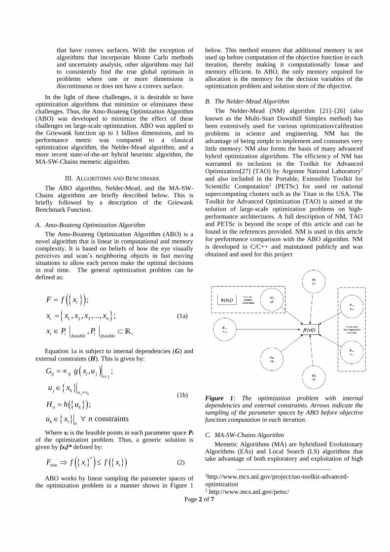
ABO works by linear sampling the parameter spaces of the optimization problem in a manner shown in Figure 1

below. This method ensures that additional memory is not used up before computation of the objective function in each iteration, thereby making it computationally linear and memory efficient. In ABO, the only memory required for allocation is the memory for the decision variables of the optimization problem and solution store of the objective.

B. The Nelder-Mead Algorithm

The Nelder-Mead (NM) algorithm [21]–[26] (also

known as the Multi-Start Downhill Simplex method) has

been extensively used for various optimization/calibration

problems in science and engineering. NM has the

advantage of being simple to implement and consumes very

little memory. NM also forms the basis of many advanced

hybrid optimization algorithms. The efficiency of NM has

warranted its inclusion in the Toolkit for Advanced

Optimization[27] (TAO) by Argonne National Laboratory1

and also included in the Portable, Extensible Toolkit for

Scientific Computation2 (PETSc) for used on national

supercomputing clusters such as the Titan in the USA. The

Toolkit for Advanced Optimization (TAO) is aimed at the

solution of large-scale optimization problems on high-

performance architectures. A full description of NM, TAO

and PETSc is beyond the scope of this article and can be

found in the references provided. NM is used in this article

for performance comparison with the ABO algorithm. NM

is developed in C/C++ and maintained publicly and was

obtained and used for this project

Figure 1: The optimization problem with internal dependencies and external constraints. Arrows indicate the sampling of the parameter spaces by ABO before objective function computation in each iteration.

C. MA-SW-Chains Algorithm

Memetic Algorithms (MA) are hybridized Evolutionary Algorithms (EAs) and Local Search (LS) algorithms that take advantage of both exploratory and exploitation of high

1http://www.mcs.anl.gov/project/tao-toolkit-advanced-

optimization 2 http://www.mcs.anl.gov/petsc/

Page 3 of 7

dimensional problems [28]. However, many LS methods do not perform well on high dimensional problems. This led to the development of an MA with LS method that performs well on both very large dimensional problems, the MA-SW-Chains algorithm [29]. MA-SW-Chains combines the classic scalable Solis Wets’ algorithm with stochastic MA for continuous optimization (MA-CMA-Chains) for high dimensional problems [28], [29]. This works by chaining each global search agent to different individual local search agents based on its features.

The MA-SW-Chains algorithm was adjudged the overall best and winner of the large-scale global optimization session in the IEEE Congress on Evolutionary Computation (2010) competition, outperforming known algorithms such as the DECC-CG, and MLCC algorithms [28], [29]. A parallel implementation of the MA-SW-Chains on GPUs significantly reduces the computational time required for very high dimensional problems, and their baseline results would be compared to the ABO algorithm.

D. Griewank Benchmark Test Function

The Griewank function is a classical optimization

benchmark function for unlimited dimensions [12], [19],

[30]–[33]. It has many widespread local minima, which are

evenly distributed. It is usually evaluated in the

domain . It is defined by:

(3)

With a global optimum at:

(4)

The Griewank function for one and two dimensions are

shown below (Figure 1 and 2), showing the many

widespread local minima:

Figure 1: Griewank function in 2-D on the domain xi ∈ [-

50, 50]3.

3Image source: http://www-optima.amp.i.kyoto-

u.ac.jp/member/student/hedar/Hedar_files/TestGO_files/Pa

ge1905.htm

(a)

(b)

Figure 2: The Griewank function in 1-D. (a) on the typical

domain of xi ∈ [-600, 600]. (b) Zoomed-in of the Griewank

function on the domain xi ∈ [0, 100]4.

IV. EXPERIMENTS WITH ABO, NM, AND MA-SW-CHAINS

ABO and NM algorithms were applied to the Griewank function for different dimensions and the following performance characteristics were recorded:

Random Access Memory (RAM) usage

Compute Wall Time

Number of Function Evaluations

Objective Function Values

The test platform for this experiment was a general-

purpose laptop computer with i7-6700HQ @ 2.6 GHz with 16GB of RAM running on 128GB SSD with Windows 10 Home operating system. The development platform was Visual Studio 2015 community. The program is compiled in Release x64 bit mode to allow for more RAM usage. The experiment was compiled for single threaded applications.

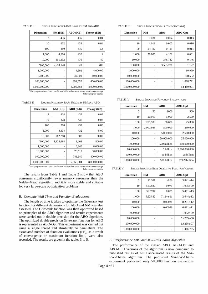
A. Random Access Memory (RAM) usage

To assess the RAM consumed by each algorithm, Process Explorer Utility was employed to measure the amount of memory consumed by ABO or NM algorithms. The results are given in the tables 1 and 2.

4 Images curtesy of Math World:

http://mathworld.wolfram.com/GriewankFunction.html

Page 4 of 7

TABLE I. SINGLE PRECISION RAM USAGE BY NM AND ABO

Dimension NM (KB) ABO (KB) Theory (KB)

2 436 436 0.01

10 432 438 0.04

100 480 436 0.4

1,000 4,368 432 4

10,000 391,332 476 40

a100,000 5,510,120 820 400

1,000,000 - 4,292 4,000.00

10,000,000 - 39,500 40,000.00

100,000,000 - 391,052 400,000.00

1,000,000,000 - 3,906,688 4,000,000.00

a NM program crashes due to insufficient RAM; values show last recorded resource usage

before program crashes.

TABLE II. DOUBLE PRECISION RAM USAGE BY NM AND ABO

Dimension NM (KB) ABO (KB) Theory (KB)

2 428 432 0.02

10 428 436 0.08

100 508 432 0.80

1,000 8,304 432 8.00

10,000 782,268 508 80.00

a100,000 5,828,688 1,208 800.00

1,000,000 - 8,248 8,000.00

10,000,000 - 78,512 80,000.00

100,000,000 - 781,640 800,000.00

1,000,000,000 - 7,965,384 8,000,000.00

a NM program crashes due to insufficient RAM; values show last recorded resource usage

before program crashes.

The results from Table 1 and Table 2 show that ABO

consumes significantly fewer memory resources than the

Nelder-Mead algorithm, and it is more stable and suitable

for very large-scale optimization problems.

B. Compute Wall Time and Function Evaluations

The length of time it takes to optimize the Griewank test function for different dimensions for ABO and NM was also assessed. The Griewank function was then optimized based on principles of the ABO algorithm and results experiments were carried out in double precision for the ABO algorithm. The optimized double precision Griewank function for ABO is represented as ABO-Opt. This experiment was carried out using a single thread and absolutely no parallelism. The associated number of function evaluations (FE), as a result of convergence or maximum iteration limit, were also recorded. The results are given in the tables 3 to 5.

TABLE III. SINGLE PRECISION WALL TIME (SECONDS)

Dimension NM ABO ABO-Opt

2 0.031 0.004 0.013

10 4.011 0.005 0.016

100 29.187 0.121 0.014

1,000 59.886 4.101 0.031

10,000 - 376.782 0.146

100,000 - 33,505.231 1.127

1,000,000 - - 10.969

10,000,000 - - 108.532

100,000,000 - - 1,068.721

1,000,000,000 - - 64,489.001

TABLE IV. SINGLE PRECISION FUNCTION EVALUATIONS

Dimension NM ABO ABO-Opt

2 50 1000 500

10 20,013 5,000 2,500

100 200,103 50,000 25,000

1,000 2,000,985 500,000 250,000

10,000 - 5,000,000 2,500,000

100,000 - 50,000,000 25,000,000

1,000,000 - 500 million 250,000,000

10,000,000 - 5 billion 2,500,000,000

100,000,000 - 50 billion 25 billion

1,000,000,000 - 500 billion 250.9 billion

TABLE V. SINGLE PRECISION BEST OBJECTIVE FUNCTION VALUES

Dimension NM ABO ABO-Opt

2 11.381 0.00 3.841e-14

10 5.59887 0.071 1.075e-09

100 36.5997 0.009 5.461e-13

1,000 5,625.82 7.114e-11 2.644e-12

10,000 - 0.00021 8.291e-12

100,000 - 0.00986 6.081e-11

1,000,000 - - 1.092e-09

10,000,000 - - 5.4269e-06

100,000,000 - - 1.6238e-07

1,000,000,000 - - 0.0017705

C. Performance ABO and MW-SW-Chains Algorithm

The performance of the classic ABO, ABO-Opt and

ABO-GPU versions of the algorithm is now compared to

published results of GPU accelerated results of the MA-

SW-Chains algorithm. The published MA-SW-Chains

experiment performed only 500,000 function evaluations

Page 5 of 7

on 24 GB RAM computer with i7 CPU processor @ 2.8

GHz; whilst GPU version was on NVidia Titan GPU with

G GB RAM and 2688 CUDA cores [29].

The ABO and ABO-Opt are run on single threads; ABO-

GPU is run on laptop gaming GPU NVidia GTX 1060 with

6 GB RAM and 1280 CUDA cores. The results of the

experiments (performed in double precision) are presented

in the tables 6 and 7.

TABLE VI. 500K FUNCTION EVALUATIONS ON CPUS (SECONDS)

Dimension

MA-SW-

Chains

(s)

ABO (s) ABO-Opt (s)

100,000 49,258 1,108.1 1.167

500,000 240,820 5,491.5 5.598

1,000,000 479,457 8,072.5 10.814

1,500,000 727,870 10,029.1 16.216

3,000,000 1,444,441 15,861.2 32.027

5,000,000 - 23,757.3 53.153

10,000,000 - 43,196.5 108.532

100,000,000 - 396,120.3 1,068.721

1,000,000,000 - 4,324,500 64,489.102

TABLE VII. 500K FUNCTION EVALUATIONS ON GPUS (SECONDS)

Dimension

GPU

MA-SW-

Chains

GPU ABO Speed-Up

100,000 1,086.7 2.112 514x

500,000 3,460.8 2.862 1,209x

1,000,000 4,332.5 4.091 1,056x

1,500,000 5,519.2 5.174 1,066x

3,000,000 8,639.8 7.544 1,145x

V. COMPUTE AND MEMORY COMPLEXITY OF ABO

ABO algorithm was designed from ground-up to be

compute and memory efficient. For single threaded

applications, the best and worst for compute efficiency (Ec)

of ABO for N decision variables is O(mN1), where m is an

intrinsic property dependent on the sampling rate and is

defined by:

(5)

Similarly, space (memory) efficiency (Em) of ABO for

single threaded applications for N decision variables is:

(6)

The best case occurs when the parameter spaces are

uniform having the same upper and lower bounds with s =

1; the worst case is where each decision variable has

different parameter spaces.

Theoretically, the parallel implementation of ABO

reduces the compute complexity O(mN1) to O(m), whilst

the space complexity increases linearly by an additional N

from O(sN1) to O[(s+N)N1]. Thus, they are given by:

(7)

(8)

Thus, in general, by comparing Equation 5 and 6, the

compute and space efficiency of ABO algorithm can be put

in a generic form be given by:

(9)

To show the efficacy of the ABO algorithm, the

theoretical memory required for the Griewank function and

the one used by the algorithm is measured and shown

below. Also, the measured computation speed of ABO as

compared to NM gives proof of its linear compute time (see

Figure 4 and Figure 5).

Figure 1: Measured Computational Efficiency of NM

and ABO algorithms

The theoretical memory consumption of ABO is

estimated by the bytes taken by the number of decision

variables w.r.t the precision (single: 4 bytes or double: 8

bytes). Thus, for single precision: RAM = 4 bytes x

decision variables. The results are shown in Table 1 and

Table 2, as well as Figure 6 and Figure 7. It can further be

seen that as the physical RAM limit was approached, the

ABO memory usage tapered, probably because the

Windows OS uses a paging system to accommodate for

excess RAM demand. Also, the RAM used by ABO

remained fairly constant for smaller numbers of decision

variables before becoming linear at 100,000 decision

variables; this is probably due to the resources used by the

other components of the software.

Page 6 of 7

NM algorithm memory resource usage rises quickly and

crashes after 10,000 decision variables. This is because a

quick analysis shows NM algorithm have a memory (space)

complexity of O[N2 + 6N + 1], thus even single precision

requires about 40 GB of RAM for 100,000 decision

variables; making it impossible to run on a general laptop.

Therefore, for large parameter calibration/optimization, NM

is on plausible on supercomputing clusters with high RAM

availability. This contrast sharply with ABO which needs

only 400 KB of RAM for 100,000 parameters.

Figure 2: Number of Function Evaluations to Convergence

of NM and ABO algorithms

Figure 3: Measured Single Precision Memory Resource

Usage of NM and ABO on Griewank Function

The results from above go to prove that the ABO

algorithm is both computationally and memory linearly

efficient. It is hoped that the algorithm can be applied to

many optimization functions and applications.

Figure 4: Measured Double Precision Memory Resource

Usage of NM and ABO on Griewank Function

VI. CONCLUSION

Amo-Boateng Optimization Algorithm (ABO) is a novel

compute and memory efficient algorithm for

optimization/calibration that was developed to address the

inherent challenges faced by current algorithms in large and

very large scale problems. In particular, given that recent

advances in computing hardware and our general

understanding of our environment have led to the

development of very large-scale optimization/calibration

models, the need for very fast efficient algorithms is

imperative.

Amongst other challenges stated in this article, these

models, however, can only be solved on HPC clusters and

supercomputers, given that the current existing

optimization algorithms require very large memory

resources, and are computationally intensive. A novel

algorithm (ABO) that is both compute and space linearly

efficient, O(αN1), has been developed. This paper shows

how the Wall Wait Time and Memory Resources used

proves that ABO is efficient linearly. In particular, by

comparing the memory used by ABO to the theoretical

minimum memory resources that can be used, and finding

these to be similar. The linear efficiency of ABO opens up

compute speeds that are only available in supercomputing

clusters and allows for solving larger problem sizes on

ordinary laptops and embedded systems.

It is the author’s hope that ABO will be useful in all

fields of science, engineering, drug research, finance,

artificial intelligence, etc. and will accelerate the time to

discovery, prototyping, and market of new developments in

these fields. It is deemed that with the widespread adoption

of ABO, Super speeds with Zero-RAM can be achieved

lowering barriers of entry and accelerating the pace of

innovation in various fields. This is because the novel

algorithm allows those speeds to be attained with zero

Page 7 of 7

additional RAM, except those required for storing the

solution.

REFERENCES

[1] D. W. Hillis, “Optimization problems,” Nature, vol. 330, no. 5, pp. 27–28, 1987.

[2] A. Delévacq, P. Delisle, M. Gravel, and M. Krajecki, “Parallel Ant Colony Optimization on Graphics Processing Units,” J. Parallel Distrib. Comput., vol. 73, no. 1, pp. 52–61, Jan. 2013.

[3] J. Parker, U. Kim, P. Kitanidis, M. Cardiff, X. Liu, and G. Beyke, “Stochastic cost optimization of DNAPL remediation – Method description and sensitivity study,” Environ. Model. Softw., vol. 38, pp. 74–88, Dec. 2012.

[4] J. Yan, H. Tiesong, H. Chongchao, W. Xianing, and G. Faling, “A shuffled complex evolution of particle swarm optimization algorithm,” in Adaptive and Natural Computing Algorithms, 2007, pp. 341–349.

[5] Y. Tang, P. Reed, and T. Wagener, “How effective and efficient are multiobjective evolutionary algorithms at hydrologic model calibration?,” Hydrol. Earth Syst. Sci., vol. 10, no. 2, pp. 289–307, 2006.

[6] G. F. Laniak, G. Olchin, J. Goodall, A. Voinov, M. Hill, P. Glynn, G. Whelan, G. Geller, N. Quinn, M. Blind, S. Peckham, S. Reaney, N. Gaber, R. Kennedy, and A. Hughes, “Integrated environmental modeling: A vision and roadmap for the future,” Environ. Model. Softw., vol. 39, pp. 3–23, Jan. 2013.

[7] W. Wenzel and K. Hamacher, “Adaptation in Stochastic tunneling global optimization of complex potential energy landscapes,” EPL (Europhysics Lett., vol. 74, no. 6, p. 944, Apr. 2006.

[8] C. Schulz, “Efficient local search on the GPU—Investigations on the vehicle routing problem,” J. Parallel Distrib. Comput., vol. 73, no. 1, pp. 14–31, Jan. 2013.

[9] B. A. Berg, “Locating global minima in optimization problems by a random-cost approach,” Nature, vol. 361, pp. 708–710, 1993.

[10] M. Mahdavi, M. Fesanghary, and E. Damangir, “An improved harmony search algorithm for solving optimization problems,” Appl. Math. Comput., vol. 188, no. 2, pp. 1567–1579, May 2007.

[11] K. S. Lee and Z. W. Geem, “A new structural optimization method based on the harmony search algorithm,” Comput. Struct., vol. 82, no. 9–10, pp. 781–798, Apr. 2004.

[12] W. Chu, X. Gao, and S. Sorooshian, “A new evolutionary search strategy for global optimization of high-dimensional problems,” Inf. Sci. (Ny)., vol. 181, no. 22, pp. 4909–4927, 2011.

[13] Z. Yang, K. Tang, and X. Yao, “Large scale evolutionary optimization using cooperative coevolution,” Inf. Sci. (Ny)., vol. 178, no. 15, pp. 2985–2999, Aug. 2008.

[14] Y. Hung and W. Wang, “Accelerating parallel particle swarm optimization via GPU,” Optim. Methods Softw., vol. 27, no. 1, pp. 33–51, Feb. 2012.

[15] D. Lu, M. Ye, M. C. Hill, E. P. Poeter, and G. P. Curtis, “A computer program for uncertainty analysis integrating regression and Bayesian methods,” Environ. Model. Softw., vol. 60, pp. 45–56, Oct. 2014.

[16] S. Navlakha and Z. Bar-joseph, “Algorithms in nature : the convergence of systems biology and computational thinking,” Mol. Syst. Biol., vol. 7, no. 546, pp. 1–11, 2011.

[17] F. Kang, J. Li, and H. Li, “Artificial bee colony algorithm and pattern search hybridized for global optimization,” Appl. Soft Comput., vol. 13, no. 4, pp. 1781–1791, Apr. 2013.

[18] J. a. Vrugt, H. V. Gupta, W. Bouten, and S. Sorooshian, “A Shuffled Complex Evolution Metropolis algorithm for optimization and uncertainty assessment of hydrologic model parameters,” Water Resour. Res., vol. 39, no. 8, p. n/a-n/a, Aug. 2003.

[19] Q. Y. Duan, V. K. Gupta, and S. Sorooshian, “Shuffled complex evolution approach for effective and efficient global minimization,” J. Optim. Theory Appl., vol. 76, no. 3, pp. 501–521, Mar. 1993.

[20] N. Muttil, S. Y. Liong, and O. Nesterov, “A Parallel Shuffled Complex Evolution Model Calibrating Algorithm to Reduce Computational Time,” in MODSIM 2007: International Congress On Modelling And Simulation: Land, Water, And Environmental Management: Integrated Systems For Sustainability (2007), 2007, pp. 1940–1946.

[21] N. Pham and B. M. Wilamowski, “Improved Nelder Mead ’ s Simplex Method and Applications,” vol. 3, no. 3, pp. 55–63, 2011.

[22] S. Singer, “Complexity Analysis of Nelder – Mead Search,” pp. 185–196, 1999.

[23] K. I. M. McKinnon, “Convergence of the Nelder--Mead Simplex Method to a Nonstationary Point,” SIAM J. Optim., vol. 9, no. 1, pp. 148–158, Jan. 1998.

[24] J. A. Nelder and R. Mead, “A simplex method for function minimization,” Comput. J., vol. 7, no. 4, pp. 303–318, Jan. 1965.

[25] T. Ye and S. Kalyanaraman, “A Recursive Random Search Algorithm for Black-box Optimization,” no. x, pp. 1–24.

[26] D. Xu, W. Wang, K. Chau, C. Cheng, and S. Chen, “Comparison of three global optimization algorithms for calibration of the Xinanjiang model parameters,” J. Hydroinformatics, 2012.

[27] T. Munson, J. Sarich, S. Wild, S. Benson, and L. C. McInnes, “TAO 2.0 Users Manual,” ANL/MCS-TM-322, 2012.

[28] D. Molina, M. Lozano and F. Herrera, "MA-SW-Chains: Memetic algorithm based on local search chains for large scale continuous global optimization," IEEE Congress on Evolutionary Computation, Barcelona, 2010, pp. 1-8. doi: 10.1109/CEC.2010.5586034

[29] Miguel Lastra, Daniel Molina, José M. Benítez, “A high performance memetic algorithm for extremely high-dimensional problems”, Information Sciences, Volume 293, 2015, Pages 35-58, ISSN 0020-0255, http://dx.doi.org/10.1016/j.ins.2014.09.018.

[30] M. Zambrano-Bigiarini and R. Rojas, “A model-independent Particle Swarm Optimisation software for model calibration,” Environ. Model. Softw., vol. 43, pp. 5–25, May 2013.

[31] F. Zhao and J. Zhang, “An Improved Shuffled Complex Evolution Algorithm and Its Performance Analysis,” Journal Comput. Inf. Syst., vol. 20, no. 61064011, pp. 8495–8502, 2012.

[32] X. Li, K. Tang, M. N. Omidvar, Z. Yang, and K. Qin, “Benchmark Functions for the CEC ’ 2013 Special Session and Competition on Large-Scale Global Optimization,” Australia, 2013.

[33] B. a. Tolson and C. a. Shoemaker, “Dynamically dimensioned search algorithm for computationally efficient watershed model calibration,” Water Resour. Res., vol. 43, no. 1, p. n/a-n/a, Jan. 2007.