1

Super-Resolution for Hyperspectral andMultispectral Image Fusion Accounting for

Seasonal Spectral VariabilityRicardo Augusto Borsoi, Tales Imbiriba, Member, IEEE, José Carlos Moreira Bermudez, Senior Member, IEEE

Abstract—Image fusion combines data from different hetero-geneous sources to obtain more precise information about anunderlying scene. Hyperspectral-multispectral (HS-MS) imagefusion is currently attracting great interest in remote sensingsince it allows the generation of high spatial resolution HS images,circumventing the main limitation of this imaging modality.Existing HS-MS fusion algorithms, however, neglect the spectralvariability often existing between images acquired at differenttime instants. This time difference causes variations in spectralsignatures of the underlying constituent materials due to differentacquisition and seasonal conditions. This paper introduces anovel HS-MS image fusion strategy that combines an unmixing-based formulation with an explicit parametric model for typicalspectral variability between the two images. Simulations withsynthetic and real data show that the proposed strategy leads toa significant performance improvement under spectral variabilityand state-of-the-art performance otherwise.

Index Terms—Hyperspectral data, multispectral data, end-member variability, seasonal variability, super-resolution, imagefusion.

I. INTRODUCTION

Hyperspectral (HS) imaging devices are non-conventionalsensors that sample the observed electromagnetic spectra athundreds of contiguous wavelength intervals.

This spectral resolution makes HS imaging an importanttool for identification of the materials present in a scene, whathas attracted interest in the past two decades. Hyperspectralimages (HSIs) are now at the core of a vast and increasingnumber of remote sensing applications such as land useanalysis, mineral detection, environment monitoring, and fieldsurveillance [1], [2].

However, the high spectral resolution of HSIs does not comewithout a compromise. Since the radiated light observed atthe sensor must be divided into a large number of spectralbands, the size of each HSI pixel must be large enough toattain a minimum signal to noise ratio. This leads to imageswith low spatial resolution [3]. Multispectral (MS) sensors,on the other hand, provide images with much higher spatialresolution, albeit with a small number of spectral bands.

One approach to obtain images with high spatial and spec-tral resolution consists in combining HS and MS images (MSI)

This work has been supported by the National Council for Scientific andTechnological Development (CNPq).

R.A. Borsoi, T. Imbiriba and J.C.M. Bermudez are with the Depart-ment of Electrical Engineering, Federal University of Santa Catarina, Flo-rianópolis, SC, Brazil. e-mail: raborsoi@gmail.com; talesim@gmail.com;j.bermudez@ieee.org.

Manuscript received Month day, year; revised Month day, year.

of the same scene, resulting in the so-called HS-MS imagefusion problem [4]. Several algorithms have been proposed tosolve this problem.Early approaches were based on componentsubstitution or on multiresolution analysis. In the former, acomponent of the HS image in some feature space is replacedby a corresponding component of the MS image [5]. In thelatter, high-frequency spatial details obtained from the MSimage are injected into the HS image [6], [7]. These techniquesgeneralize Pansharpening algorithms, which combine an HSIwith a single complementary monochromatic image [8].

More recently, subspace-based formulations have becomethe leading approach to solve this problem, exploring thenatural low-dimensional representation of HSIs as a linearcombination of a small set of basis vectors or spectralsignatures [4], [9], [10], [11]. Many approaches have beenproposed to perform image fusion under this formulation.For instance, Bayesian formulations have been proposed tosolve this problem as a maximum a posteriori estimationproblem [12], as the solution to a Sylvester equation [13],or by considering different forms of sparse representations onlearned dictionaries [14], [15]. Other works propose a matrixfactorization formulation, using for instance sparse [16], [17]or spatial regularizations [18], or processing local imagepatches individually [19]. Other approaches use unsupervisedformulations which jointly estimate the set of basis vectors andtheir coefficients [20], [21]. More recently, tensor factorizationmethods have also been proposed to solve the image fusionproblem by exploring the natural representation of HSIs as3-dimensional tensors [22], [23].

Although platforms carrying both HS and MS imagingsensors are becoming more common in recent years, theirnumber is still considerably limited [24], [25]. However, theincreasing number of optical satellites orbiting the Earth (e.g.Sentinel, Orbview, Landsat and Quickbird missions) providesa large amount of MS data, which can be exploited to performimage fusion using HS images acquired on board of differentmissions [4]. This scenario provides the greatest potential forthe use of HS-MS fusion in practical applications. Further-more, the short revisit cycles of these satellites provide MSimages at short subsequent time instants. These MS imagescan be used to generate HS image sequences with a hightemporal resolution (what has been already done with Landsatand MODIS data [26], [27], [28], [29], [30]).

Though combining images from different sensors providesa great opportunity for applying image fusion algorithms, itintroduces a challenge that has been largely neglected. Since

arX

iv:1

808.

1007

2v1

[cs

.CV

] 3

0 A

ug 2

018

2

the HS and MS images are observed at different time instants,their acquisition conditions (e.g. atmospheric and illumination)can be significantly different from one another. Furthermore,seasonal changes can make the spectral signature of thematerials in the HS image change significantly from thosein the corresponding MSI. These factors have been ignoredin image fusion algorithms proposed to date, and can have asignificant impact on the solution of practical problems.

In this paper, we propose a new image fusion methodaccounting for spectral variability between the images, whichcan be caused by both acquisition (e.g. atmospheric, illu-mination) or seasonal changes. Differently from existing ap-proaches, we allow the high-resolution images underlying theobserved HS and MS images to be different from one another.Employing a subspace/unmixing-based formulation, we usea unique set of endmembers for each image, employing aparametric model to represent the variability of the spectralsignatures. The proposed algorithm, which is called HS-MSimage Fusion with spectral Variability (FuVar), estimates thesubspace components (endmembers and abundance maps) ofthe high-resolution images using an alternating optimizationapproach, making use of the Alternating Direction Methodof Multipliers to solve each subproblem. Simulation resultswith synthetic and real data show that the proposed approachperforms similarly or better than state-of-the-art methods forimages acquired under the same conditions, and much betterwhen there is spectral variability between them.

The paper is organized as follows. In Section II, theHS and MS observation process is presented, and a newmodel to represent spectral variability between these imagesis proposed. The proposed FuVar algorithm is introduced inSection III. Experimental results with synthetic and real remotesensing images are presented in Section IV. Finally, Section Vconcludes the paper.

II. SPECTRAL VARIABILITY IN IMAGE FUSION

Let Yh ∈ RLh×N be an observed low spatial resolution HSIwith Lh bands and N pixels, and Ym ∈ RLm×M an observedlow spectral resolution MSI with Lm bands and M pixels, withLm < Lh and N < M . The image fusion problem consists ofestimating an underlying image Z ∈ RLh×M with high spatialand spectral resolutions, given Yh and Ym.

A common approach to solve this problem is based onspectral unmixing using the linear mixture model (LMM). TheLMM assumes that the spectral representation of an observedimage can be decomposed as a convex combination of a smallnumber P Lh of spectral signatures (called endmembers)of pure materials in the scene [9]. Let

Z = MA (1)

be the LMM for the underlying image Z. In (1), the columnsof M ∈ RLh×P are the spectral signatures of the P end-members, and each column of A ∈ RP×M is the vector offractional abundances for the corresponding pixel of Z.

Unmixing-based formulations successfully exploit the re-duced dimensionality of the problem since only matrices Mand A (which are much smaller than Z) need to be estimated.

Furthermore, a good estimate of M for the fusion problemcan be obtained directly from Yh due to its high spectralresolution [18]. Other subspace estimation techniques, suchas SVD or PCA, can also be employed to represent Z.However, the LMM is usually preferred for its connection withthe physical mixing process and for the better performanceempirically verified in practice [4], [18].

The HS-MS image fusion literature assumes that all ob-served images are acquired at exactly the same conditions.This consideration allows both the HS and the MS imagesto be directly related to a unique underlying image Z. This,however, is a major limitation of existing methodologies sincea vast amount of data available for processing may comefrom sensors on board of different instruments or missions(e.g. AVIRIS and Sentinel images). In such scenarios, theacquisition conditions can be very different for HS and MSimages, especially when there is a significant time intervalbetween their capture. Such situation is commonly encoun-tered when data provided by several different MS sensorsis used to generate high temporal resolution sequences. Theuse of different sensors introduces variability in the spectralsignatures of the observed images due to, for instance, varyingillumination, different atmospheric conditions, or seasonalspectral variability of the materials in the scene (e.g. in thecase of vegetation analysis) [31], [32]. These effects cannotbe adequately modeled by unmixing or subspace formulationsthat assume a single underlying image Z for both the HSand MS images. These methods assume that the underlyingmaterials M have the same spectral signatures in both im-ages, and thus can be decomposed using the same subspacecomponents [20], [18], [33]. In the following, we propose anew model that accounts for the effects of spectral variabilityin HS-MS image fusion.

A. The proposed model

Consider distinct high-resolution images Zh and Zm, bothwith Lh bands and M pixels, corresponding to the observedHSI and MSI, respectively. These high resolution (HR) imagescan be different due to seasonal variability effects. We thendecompose Zh and Zm as

Zh = MhA , Zm = MmA (2)

where A ∈ RP×M is the fractional abundance matrix, assumedcommon to both images, and Mh, Mm ∈ RLh×P are theendmember matrices of the HSI and MSI, respectively. Mh

and Mm can be different to account for spectral variability.Using (2), we assume that the observed HSI and MSI are

generated according to

Yh = MhAFD +Nh

Ym = RMmA+Nm

(3)

where F ∈ RM×M accounts for optical blurring due tothe sensor point spread function, D ∈ RM×N is a spatialdownsampling matrix, R ∈ RLm×Lh is a matrix containingthe spectral response functions (SRF) of each band of theMS instrument. Nh ∈ RLh×N and Nm ∈ RLm×M representadditive noise.

3

Matrix Mh can be estimated from the observed HSI Yh

using endmember extraction or subspace decomposition. How-ever, the same is not true for the estimation of Mm since theMSI Ym has low spectral resolution. To address this issue, wepropose to write Mm as a function of Mh using a specificmodel for spectral variability.

Different parametric models have been recently proposedto account for spectral variability in hyperspectral unmixing.The extended LMM proposed in [34] allows the scaling ofeach endmember spectral signature by a constant. This modeleffectively represents illumination and topographic variations,but is limited in capturing more complex variability effects.The perturbed LMM proposed in [35] adds an arbitraryvariation matrix to a reference endmember matrix. This modellacks a clear connection to the underlying physical phenomena.The generalized LMM (GLMM), recently proposed in [36],accounts for more complex spectral variability effects byconsidering an individual scaling factor for each spectralband of the endmembers. This model introduces a connectionbetween the amount of spectral variability and the amplitudeof the reference spectral signatures, agreeing with practicalobservations.

Considering the GLMM, we propose to model the multi-spectral endmember matrix Mm as a function of the end-members extracted from the HSI as

Mm = Ψ Mh (4)

where Ψ ∈ RLh×P is a matrix of positive scaling factorsand denotes the Hadamard product. Then, the image fusionproblem problem can finally be formulated as the problem ofrecovering the matrices Mh, Ψ and A from the observed HSand MS images Yh and Ym.

III. THE IMAGE FUSION PROBLEM

Considering the observation model in (3) and assumingthat matrices Mh, F , D and R are known or estimatedpreviously, the image fusion problem reduces to estimatingthe variability and abundance matrices Ψ and A. Therefore,we propose to solve the image fusion problem through thefollowing optimization problem:

A∗,Ψ∗ = argminA≥0,Ψ≥0

1

2‖Yh −MhAFD‖2F

+1

2‖Ym −R(Ψ Mh)A‖2F + λAR(A)

+λ12‖Ψ− 1L1>P ‖2F +

λ22‖H`Ψ‖2F (5)

where parameters λ1, λ2 and λA balance the contributionsof the different regularization terms to the cost function. Thelast two terms are regularizations over Ψ. The first of themcontrols the amount of spectral variability by constraining Ψto be close to unity. The second enforces spectral smoothnessby making H` a differential operator.R(A) is a regularizationover A to enforce spatial smoothness, and is given by

R(A) =(‖Hh(A)‖2,1 + ‖Hv(A)‖2,1

)where the linear operators Hh and Hv compute the first-order horizontal and vertical gradients of a bidimensional

signal, acting separately for each material of A. The spatialregularization in the abundances is promoted by a mixedL2,1 norm of their gradient, where ‖X‖2,1 =

∑Nn=1 ‖xn‖2.

This norm is used to promote sparsity of the gradient acrossdifferent materials (i.e. to force neighboring pixels to behomogeneous in all constituent endmembers). The L1 normcan also be used, leading to the Total Variation regularization,where ‖X‖1 =

∑Nn=1 ‖xn‖1 [37].

Although the problem defined in (5) is non-convex withrespect to both A and Ψ, it is convex with respect toeach of the variables individually. Thus, we propose to usean alternating least squares strategy by minimizing the costfunction iteratively with respect to each variable in order tofind a local stationary point of (5). This solution is presentedin Algorithm 1, and the individual steps are detailed in thefollowing subsections.

Algorithm 1: FuVarInput : Ym, Yh, F , D, R parameters P , λA, λ1, λ2.Output: The estimated high-resolution images Zh

and Zm.1 Estimate Mh from Yh using an endmember extraction

algorithm;2 Initialize Ψ(0) = 1L1>P ;3 Initialize A with a bicubic interpolation of the FCLS

estimative ;4 Set i = 0 ;5 while stopping criterion is not satisfied do6 i = i+ 1 ;7 Compute A(i) by solving (6) using Ψ ≡ Ψ(i−1);8 Compute Ψ(i) by solving (45) using A ≡ A(i) ;9 end

10 return Zh = MhA(i), Zm = (Ψ(i) Mh)A

(i) ;

A. Optimizing w.r.t. A

To solve problem (5) with respect to A for a fixed Ψ, wedefine the following optimization problem rewriting the termsin (5) that depend on A:

A∗ = argminA

1

2‖Yh −MhAFD‖2F + ιR+

(A)

+1

2‖Ym −R(Ψ Mh)A‖2F

+ λA(‖Hh(A)‖2,1 + ‖Hv(A)‖2,1

)(6)

where ιR+(·) is the indicator function of R+ (i.e. ιR+

(a) = 0if a ≥ 0 and ιR+

(a) = ∞ if a < 0) acting component-wiseon its input, and enforces the abundance positivity constraint.

Since problem (6) is not separable w.r.t. the pixels neitherdifferentiable due to the presence of the L2,1 norm we resortto a distributed optimization strategy, namely the alternatingdirection method of multipliers (ADMM). Specifically, thecost function in (6) must be represented in the followingform [38]

minx,w

f(x) + g(w)

∣∣∣Ax+ Bw = c, (7)

4

where f : Ra → R+ and g : Rb → R+ are closed, proper andconvex functions, and x ∈ Ra, w ∈ Rb, c ∈ Rc, A ∈ Rc×a,B ∈ Rc×b.

Using the scaled formulation of the ADMM [38, Sec. 3.1.1],the augmented Lagrangian associated with (7) is given by

L(x,w,u) = f(x) + g(w) +ρ

2

∥∥Ax+ Bw − c+ u∥∥22

(8)

with u ∈ Rc the scaled dual variable, and ρ > 0. The ADMMconsists of updating the variables x, w and u sequentially.Denoting the primal and dual variables at the k-th iterationof the algorithm by x(k), w(k) and u(k), the ADMM can beexpressed as

x(k+1) ∈ argminxL(x,w(k),u(k))

w(k+1) ∈ argminwL(x(k),w,u(k))

u(k+1) = u(k) +Ax(k+1) + Bw(k+1) − c.

(9)

To represent optimization problem (6) in the form of (7),we define the following variables:

B>1 = D>F>B>2

B2 = MhA

B3 = A

B4 = Hh(B3)

B5 = Hv(B3)

B6 = A.

(10)

The optimization problem (6) is then rewritten as

A∗ = argminA

1

2‖Yh −B1‖2F + λA

(‖B4‖2,1 + ‖B5‖2,1

)+

1

2‖Ym −R(Ψ Mh)A‖2F + ι+(B6) (11)

subject to the equations in (10)

This problem is equivalent to (7), with c = 0, x given by (12),where vec(·) is the vectorization operator, and w, A and Bgiven as follows (Eqs. (13)–(15))

w = vec(A) (13)

A =

−I repL(D

>F>) 0 0 0 00 P> 0 0 0 00 0 I 0 0 00 0 −Hh I 0 00 0 −Hv 0 I 00 0 0 0 0 I

(14)

where P> is a permutation matrix that performs the transpo-sition of the vectorized HSI, that is, P>vec(B>2 ) = vec(B2),and

B =

0

−repM (Mh)−I00−I

(15)

where repM (B) are block diagonal matrices with M repeatsof matrix B in the main diagonal, that is,

repM (B) =

B 0 · · · 00 B 0...

. . ....

0 0 · · · B

. (16)

Using (13)–(15) in (8), the scaled augmented Lagrangianof (11) can be written as

L(Θ) =1

2‖Yh −B1‖2F

+1

2‖vec(Ym)− repM (R(Ψ Mh))w‖2

+ λA(‖B4‖2,1 + ‖B5‖2,1

)+ ι+(B6)

+ρ

2

(‖repL(D

>F>)vec(B>2 )− vec(B>1 ) + u1‖2

+ ‖vec(B2)− repM (Mh)w + u2‖2

+ ‖vec(B3)−w + u3‖2

+ ‖vec(B4)−Hhvec(B3) + u4‖2

+ ‖vec(B5)−Hvvec(B3) + u5‖2

+ ‖vec(B6)−w + u6‖2)

(17)

where Θ = w,B1,B2,B3,B4,B5,B6,u and ui, i =1, . . . , 6 form the partition of the dual variable u with com-patible dimensions, which is given by

u =[u>1 u>2 u>3 u>4 u>5 u>6

]>. (18)

In the following, we detail the optimization of L(Θ) withrespect to each of the variables in Θ.

1) Optimizing w.r.t. w: The subproblem of minimizingL(Θ) with respect to w can be extracted from (17) byselecting the terms that depend on w:

minw

1

2‖vec(Ym)− repM (R(Ψ Mh))w‖2

+ρ

2

(‖vec(B2)− repM (Mh)w + u2‖2

+ ‖vec(B3)−w + u3‖2

+ ‖vec(B6)−w + u6‖2). (19)

Alternatively, since w is the vectorization of the abundancematrix A, we can re-write this problem for each pixel as

minan

M∑n=1

(12‖ym,n −R(Ψ Mh)an‖2

+ρ

2

(‖b2,n −Mhan + u2,n‖2

+ ‖b3,n − an + u3,n‖2

+ ‖b6,n − an + u6,n‖2)). (20)

Taking the gradients w.r.t. an and setting them equal to zeroleads to((

R(Ψ Mh))>(

R(Ψ Mh))+ ρM>

hMh + 2ρI)an

= ρ(M>

h (b2,n + u2,n) + (b3,n + u3,n)

+ (b6,n + u6,n))+(R(Ψ Mh)

)>ym,n (21)

5

x =[

vec(B>1 )> vec(B>2 )

> vec(B3)> vec(B4)

> vec(B5)> vec(B6)

>]>

(12)

and the solution is given by

a∗n = Ω−11 Ω2 (22)

with

Ω1 =(R(Ψ Mh)

)>(R(Ψ Mh)

)+ ρM>

hMh + 2ρI

Ω2 = ρ(M>

h (b2,n + u2,n) + (b3,n + u3,n) + (b6,n + u6,n))

+(R(Ψ Mh)

)>ym,n . (23)

2) Optimizing w.r.t. B1: Equivalently to Section III-A1, thesubproblem for B1 can be written as

minB1

1

2‖Yh −B1‖2F

+ρ

2‖repL(D

>F>)vec(B>2 )− vec(B>1 ) + u1‖2. (24)

Representing the last term of (24) in matrix form leads to

minB1

1

2‖Yh −B1‖2F

+ρ

2‖D>F>B>2 −B>1 + vec−1(u1)‖2F (25)

where(vec−1(u1)

)>= U1. Problem (25) is equivalent to

minB1

1

2‖Yh −B1‖2F +

ρ

2‖B2FD −B1 + U1‖2F (26)

and can be re-written individually for each pixel as

minB1

N∑n=1

(12‖yh,n − b1,n‖2

+ρ

2‖[B2FD]n − b1,n + u1,n‖2

). (27)

Thus, taking the derivative of (27) for each pixel and settingit equal to zero, we have

b∗1,n =1

1 + ρ

(yy,n + ρ[B2FD]n + ρu1,n

)(28)

for n = 1, . . . , N .

3) Optimizing w.r.t. B2: Analogously to Section III-A1, thesubproblem for B2 can be written as

minB2

ρ

2

(‖repL(D

>F>)vec(B>2 )− vec(B>1 ) + u1‖2

+ ‖vec(B2)− repM (Mh)w + u2‖2). (29)

Representing the variables in matrix form, problem (29) isequivalent to

minB2

ρ

2

(‖D>F>B>2 −B>1 +U1‖2F

+ ‖B>2 −A>M>h +U>2 ‖2F

)(30)

and can be recast to each HS band as

minB2

L∑`=1

1

2

(‖D>F>[B>2 ]` − [B>1 ]` + [U1]`‖2

‖ [B>2 ]` − [A>M>h ]` + [U>2 ]`‖2

). (31)

Taking the derivative w.r.t. each band and setting it equalto zero gives(I + FDD>F>

)[B>2 ]` = [A>M>

h ]` − [U>2 ]` + FD[B>1 ]`

− FD[U1]` (32)

for ` = 1, . . . , L. Since matrices F and D are sparse,problem (32) can be solved efficiently using iterative methodssuch as the Conjugate Gradient method, where the largematrices involved can be computed implicitly.

4) Optimizing w.r.t. B3: This subproblem is equivalent to

minB3

ρ

2

(‖vec(B3)−w + u3‖2

+ ‖vec(B4)−Hhvec(B3) + u4‖2

+ ‖vec(B5)−Hvvec(B3) + u5‖2)

(33)

whose solution w.r.t. vec(B3) leads to

vec(B3)∗ =

(I +H>hHh +H>v Hv

)−1(w − u3

+H>h vec(B4) +H>h u4

+H>v vec(B5) +H>v u5

). (34)

The dimensionality of the matrices Hh and Hv in thisproblem makes the direct inversion of the terms involvingthem in (34) impractical. However, assuming these differentialoperators are block circulant, and following the same approachas in [34] and [36], these operations can be computed effi-ciently. This is done by performing the computations with thedifferential operators and their adjoint in the Fourier domain,independently for each endmember. Denoting the convolutionmasks associated with Hh and Hv by hh and hv , respectively(see details in [34]), assuming circular boundary conditionsand using properties of the Fourier transform, the solutionin (34) can be computed equivalently as

[B3]:,:,p = F−1((F(A:,:,p − [U3]:,:,p)

+ F∗(hh) F([B4]:,:,p + [U4]:,:,p)

+ F∗(hv) F([B5]:,:,p + [U5]:,:,p))

(1M11

>M2

+ |F(hh)|2 + |F(hv)|2))

(35)

for p = 1, . . . , P , where F and F−1 are the forward andinverse 2D Fourier transforms, is the elementwise division,and tensors A, U3, B4, U4, B5, U5, of size M1×M2×P arethe cube-ordered versions of the respective variables in (34).F∗ is the complex conjugate of the Fourier transform, and | · |is the modulus operator, applied elementwise to a matrix.

6

5) Optimizing w.r.t. B4: The equivalent optimization prob-lem can be written as

minB4

λA‖B4‖2,1 +ρ

2‖vec(B4)−Hhvec(B3)− u4‖2. (36)

Following the same idea as in [34], the solution of problem(36) is equivalent to the proximal operator of the L2 norm.The solution to this problem is obtained by using block softthresholding, which can then be expressed as

B∗4 = softλA/ρ

(Hhvec(B3) + u4

)(37)

where the soft operator for the L2 norm is defined as [34]

softa(b) = max(1− a

‖b‖, 0)b (38)

with softa(0) = 0, ∀a.

6) Optimizing w.r.t. B5: Equivalently, this optimizationproblem can be written as

minB5

λA‖B5‖2,1 +ρ

2‖vec(B5)−Hvvec(B3) + u5‖2 (39)

which is identical to problem (37). Following the strategyoutlined above, the solution to (39) is given by

B∗5 = softλA/ρ

(Hvvec(B3)− u5

). (40)

7) Optimizing w.r.t. B6: This optimization problem can bewritten as

minB6

ι+(B6) +ρ

2‖vec(B6)−w + u6‖2. (41)

The solution to this problem is presented in [34], and isgiven by

B∗6 = max(

vec−1(w)− vec−1(u6), 0). (42)

8) Dual update u: The dual update is given by

u(k+1) = u(k) +Ax(k+1) + Bw(k+1) − c (43)

which becomes

u1 ← u1 − vec(B>1 ) + repL(D>F>)vec(B>2 )

u2 ← u2 + P>vec(B>2 )− repM (Mh)w

u3 ← u3 + vec(B3)−w

u4 ← u4 + vec(B4)−Hhvec(B3)

u5 ← u5 + vec(B5)−Hvvec(B3)

u6 ← u6 + vec(B6)−w .

(44)

B. Optimizing w.r.t. Ψ

The optimization problem with respect to Ψ and consideringA fixed can be recast from (5) by considering only terms thatdepend on Ψ:

Ψ∗ = argminΨ≥0

1

2‖Ym −R(Ψ Mh)A‖2F

+λ12‖Ψ− 1L1>P ‖2F +

λ22‖H lΨ‖2F (45)

Analogously to Section III-A, the ADMM can be usedto split problem (45) into smaller simpler problems that aresolved iteratively. Specifically, we denote

B = Ψ Mh

x = vec(B)

w = vec(Ψ)

A = I

B = − diag(vec(Mh)) .

(46)

Then, the optimization problem (45) can be expressed as

Ψ∗ = argminΨ

1

2‖Ym −RBA‖2F + ι+(Ψ)

+λ12‖Ψ− 1L1>P ‖2F +

λ22‖H lΨ‖2F (47)

subject to B = Ψ Mh

which is equivalent to the ADMM problem.The scaled augmented Lagrangian for this problem can be

written as

L(x,w,u) = 1

2‖Ym −RBA‖2F + ι+(w)

+λ12‖Ψ− 1L1>P ‖2F +

λ22‖H lΨ‖2F

+ρ

2‖B −Ψ Mh +U‖2F . (48)

Next, we present the optimization procedures for minimizingL(x,w,u) with respect to x, w and u. The reader shouldnote, however, that the optimizations with respect to x and ware equivalent to the optimizations with respect to B and Ψ,respectively, see (46).

1) Optimizing w.r.t. B: The resulting optimization problemfor B can be written as

minB

1

2‖Ym −RBA‖2F +

ρ

2‖B −Ψ Mh +U‖2F . (49)

Taking the derivative with respect to B and setting it equalto zero leads to

1

ρR>RBAA> +B =

1

ρR>YmA>

+ Ψ Mh −U . (50)

This consists in the Sylvester equation AXB −X +C = 0.1

1In MATLABTM, X = dlyap(A,B,C) solves the equation AXB - X + C = 0,with A, B, and C with compatible dimensions but not required to be square.

7

2) Optimizing w.r.t. Ψ: The optimization problem can bewritten as

minΨ≥0

λ12‖Ψ− 1L1>P ‖2F +

λ22‖H lΨ‖2F (51)

+ρ

2‖B −Ψ Mh +U‖2F .

For simplicity, the nonnegativity constraint will be initiallyignored. Taking the derivative w.r.t. Ψ and setting it equal tozero leads to:

λ1(Ψ− 1L1>P ) + λ2H>l H lΨ

− ρ(Mh B +Mh U −Mh Mh Ψ) = 0 . (52)

The matrix equation (52) can be written in vector form as(λ1I + λ2repP (H

>l H l)

+ ρ diag(vec(Mh Mh)))

vec(Ψ) = λ11

+ ρ vec(Mh B +Mh U) (53)

which is a system of equations that can be solved efficientlysince the matrices on the left-hand side are very sparse. Finally,positivity is introduced in the solution obtained by solving thesparse system in (53) as

Ψ∗ = max(Ψ,0) . (54)

3) Dual update u: The dual update is given by

U ← U +B −Mh Ψ . (55)

IV. EXPERIMENTAL RESULTS

Three experiments were devised to illustrate the perfor-mance of the proposed method. The first one uses syntheticallygenerated images with controlled spectral variability in orderto assess the estimation performance. The second comparesthe performances of the proposed method with those of othertechniques when there is no spectral variability between theimages (i.e. acquired at the same time instant). Finally, thethird example depicts the fusion of real HS and MS imagesacquired at different time instants, thus containing spectralvariability. Details of the three examples and their experimen-tal setups are described next.

A. Experimental Setup

We compare the proposed method to three other techniques,namely: the unmixing-based HySure [18] and the CNMF [20]algorithms, and the multiresolution analysis-based GLP-HSalgorithm [7]. These methods provided the best overall fusionperformance in extensive experiments reported in survey [4].

For experiments 2 and 3, which are based on real hyper-spectral and multispectral images acquired at the same spatialresolution, two preprocessing steps were performed based onthe same procedure described in [18]. First, spectral bandswith low SNR or corresponding to water absorption spectrawere manually removed. Next, all bands of the hyperspectraland multispectral images were normalized such that the 0.999intensity quantile corresponded to a value of 1. Finally, the

HSI was denoised using the method described in [39] to yieldhigh-SNR (hyperspectral) reference images Zh [4].

For all experiments, the observed HSIs were generated byblurring the reference HSI image with a Gaussian filter withunity variance, decimating it and adding noise to obtain a 30dBSNR. The observed MSIs were obtained from the referenceMSI image by adding noise to obtain a 40dB SNR.

We fixed the number of endmembers at P = 30 for theCNMF, HySure and FuVar methods according to [4]. Theblurring kernel F was assumed to be known a priori for theHySure and FuVar methods, and Mh was estimated fromthe HSI using the VCA algorithm [40]. The regularizationparameters for the proposed method were empirically set atλA = 10−4, λ1 = 0.01 and λ2 = 104. We selected a largevalue for λ2 to have spectrally smooth variability, and a smallvalue of λ1 to allow the scaling factors Ψ to adequately fit thedata. Nevertheless, the proposed method showed to be fairlyinsensitive to the choice of parameters. We ran the alternatingoptimization process in Algorithm 1 for at most 10 iterationsor until the relative change of A and Ψ was less than 10−3.

The visual assessment of the reconstructed images is per-formed using one true-color image at the visible spectrum(with red, green and blue corresponding to 0.45, 0.56 and0.66µm) and one pseudo-color image at the infrared spec-trum (with red, green and blue corresponding to 0.80, 1.50and 2.20µm).

B. Quality measures:

We use four quality metrics previously considered in [4],[18] to evaluate the quality of the reconstructed images. Thefirst one is the peak signal to noise ratio (PSNR), computedbandwise and defined as

PSNR(Z, Z) =1

L

L∑`=1

10 log10

(M Emax(Z`,:)‖Z`,: − Z`,:‖2F

)(56)

where E· is the expected value operator and Z`,: ∈ R1×M

denotes the `-th band of Z. Larger PSNR values indicatehigher quality of spatial resconstruction, tending to infinitywhen the bandwise reconstruction error tends to zero.

The second metric is the Spectral Angle Mapper (SAM):

SAM(Z, Z) =1

M

M∑n=1

cos−1(

Z>:,nZ :,n

‖Z :,n‖2‖Z :,n‖2

). (57)

The third metric is the Erreur Relative Globale Adimen-sionnelle de Synthèse (ERGAS) [41], which provides a globalstatistical measure of the quality of the fused data with thebest value at 0:

ERGAS(Z, Z) = 100

√√√√ N

LM

L∑`=1

‖Z`,: − Z`,:‖2Fmean(Z`,:)2

(58)

where mean(·) computes the sample mean value of a signal.

8

Finally, the fourth metric is the Universal Image QualityIndex (UIQI) [42], extended to multiband images as

UIQI(Z, Z) =4

LK

L∑`=1

K∑k=1

cov(P kZ`,:,P kZ`,:)

var(P kZ`,:) + var(P kZ`,:)

× mean(P kZ`,:)mean(P kZ`,:)

mean(P kZ`,:)2 + mean(P kZ`,:)2(59)

where var(·) computes the sample variance of a signal,cov(B1,B2) computes the sample covariance between B1

and B2, and P k is a projection matrix which extracts the k-th patch with 32 × 32 pixels from the images Z`,: and Z`,:,with K being the total number of image patches. The UIQIis restricted to the interval [−1, 1], corresponding to a perfectreconstruction when equal to one.

C. Example 1

This example was designed to evaluate the algorithms ina controlled environment. The true abundance matrix A,with 100 × 100 pixels and containing spatial correlation wasgenerated using a Gaussian Random Fields algorithm. Threeendmembers with L = 244 bands were selected from theUSGS spectral library and used to construct matrix Mh. TheMS endmember matrix Mm was obtained by multiplyingMh with a matrix of scaling factors Ψ to introduce spectralvariability. Matrix Ψ was constructed by random piecewiselinear functions centered around a unitary gain. The high-resolution HS and MS images Zh and Zm were generatedfrom this data using the linear mixing model. The MS imageYm with Ll = 16 bands was then generated by applying apiecewise uniform SRF to Zm. The low-resolution HS Yh

image was generated by blurring Zh with a Gaussian filterwith unitary variance and decimating it by a factor of 4.Finally, white Gaussian noise was added to both images,resulting in SNRs of 30dB for Y h and 40dB for Ym. Both theblurring kernel F and the SRF R were assumed to be knowna priori for all algorithms.

The quantitative results for the quality of the reconstructedimages with respect to both Zh and Zm are shown in Table I.Figs. 1 and 2 provide a visual assessment of the results forthe super resolved HS and MS images Zh and Zm.

Table IEXAMPLE 1 - RESULTS FOR THE SYNTHETIC HS AND MS IMAGES.

Hyperspectral HR image Multispectral HR image

PSNR SAM ERGAS UIQI PSNR SAM ERGAS UIQI

GLP-HS 29.21 2.055 1.152 0.826 25.51 2.936 1.665 0.778HySure 31.00 1.430 1.013 0.936 33.56 1.611 0.761 0.942CNMF 36.60 0.825 0.480 0.956 28.49 2.191 1.296 0.906FuVar 42.22 0.509 0.257 0.989 42.69 0.497 0.242 0.980

1) Discussion: The results presented in Table I clearlyshow the performance gains obtained in all metrics usingthe proposed FuVar method. In terms of PSNR, the FuVaralgorithm yielded gains larger than 5dB and 9dB for Zh

and Zm, respectively. Substantial performance improvementswere also obtained for all other metrics, indicating that FuVar

Figure 1. Visual results for the hyperspectral images in Example 1.

Figure 2. Visual results for the multispectral images in Example 1.

yields more accurate spatial and spectral results, resulting inbetter image reconstruction. Visual inspection of Figs. 1 and 2shows that all methods yield reasonable results for both thevisible and infrared regions of the spectrum. However, themost accurate reconstruction is clearly provided by FuVar,which keeps a good trade-off between the smooth parts andsharp discontinuities in the image without introducing spatialartifacts or color distortions. Such defects can be seen inthe results from all other methods such as the CNMF and,especially, the HySure algorithm.

D. Example 2

This example compares the performance of the differentmethods when there is no spectral variability between theHS and MS images. We consider a dataset consisting of HSand MS images acquired above Paris with a spatial resolutionof 30m. These images were initially presented in [18] andcaptured by the Hyperion and the Advanced Land Imagerinstruments on board the Earth Observing-1 Mission satellite.

The reference HSI, with 72 × 72 pixels and L = 128bands was blurred by a Gaussian filter with unity varianceand decimated by a factor of 3. Finally, WGN was added togenerate the observed HSI Yh with a 30dB SNR. The observedMSI Ym with Ll = 9 bands was obtained from the referenceMSI by adding WGN to achieve a 40dB SNR. The spectralresponse function R was estimated from the observed imagesusing the method described in [18].

The quantitative results for the quality of the reconstructedimages with respect to Zh are displayed in Table II. A visualassessment of the results for the super-resolved HS image Zh

is presented in Fig. 3.1) Discussion: Although the proposed method estimates

the matrix Ψ to cope with the spectral variability oftenexisting between the HS and MS images, its performance wasstill comparable with state of the art image fusion methods

9

Table IIEXAMPLE 2 - RESULTS FOR THE PARIS IMAGE.

PSNR SAM ERGAS UIQI

GLP-HS 26.78 3.811 5.218 0.778HySure 28.78 3.060 4.169 0.844CNMF 28.08 3.432 4.529 0.818FuVar 28.97 3.156 4.016 0.848

Figure 3. Visual results for the hyperspectral images in Example 2.

when there was no spectral variability. In fact, the resultsin Table II show that FuVar yielded slightly better than thecompeting methods for all metrics but the SAM, for whichit yielded the second best and very close to the best result.The slight improvement obtained by the FuVar algorithmcan be attributed to the fact that the matrix Ψ, originallydevised to capture spectral variability, can also incorporateother modeling errors. In this particular example, such errorscan be introduced by the estimation of the spectral responsefunction R. Visually, the images displayed in Fig. 3 alsoindicate that the results obtained with all methods are verysimilar. This reconstruction similarity is in agreement with thequantitative results presented in Table II.

Lake TahoeIvanpah Playa

Figure 4. Hyperspectral and multispectral images used in Experiment 3.

E. Example 3

This example illustrates the performance of the proposedmethod when fusing HS and MS images acquired at differenttime instants, thus presenting seasonal spectral variability. Weconsider two pairs of reference hyperspectral and multispectralimages with a spatial resolution of 20m. The HS images wereacquired by the AVIRIS instrument and contained L = 173bands after pre-processing, while the MS images containingLl = 10 bands was acquired by the Sentinel-2A instrument.

The first pair of images, with 100×80 pixels, were acquiredover the Lake Tahoe area and can be seen in Fig. 4. The

HS and MS images were acquired at 04/10/2014 and at24/10/2017, respectively. The second pair of images, with80×128 pixels, were acquired over the Ivanpah Playa and arealso shown in Fig. 4. The HS and MS images were acquiredat 26/10/2015 and at 17/12/2017, respectively2. A significantspectral variability between the images can be readily verifiedin both cases. For the Lake Tahoe image, it is evidenced bythe different color hues of the ground, and by the appearenceof the crop circles, which are younger and have a lighter colorin the MSI. In the Ivanpah Playa image, a significant overalldifference is observed between the sand colors in both images.

The reference hyperspectral images were blurred by a Gaus-sian filter with unity variance and decimated by a factor of 4.Finally, WGN was added to generate the observed HSIs Yh

with a 30dB SNR. The observed MS images Ym was obtainedby adding WGN to the reference MSI to obtain a 40dB SNR.The spectral response function R obtained from calibrationmeasurements and was thus known a priori3.

The quantitative results for both images are displayed inTable III, and a visual assessment of the results for the super-resolved HS images Zh is presented in Figs. 6 and 5.

Table IIIEXAMPLE 3 - RESULTS FOR LAKE TAHOE AND IVANPAH PLAYA IMAGES.

Lake Tahoe image Ivanpah Playa image

PSNR SAM ERGAS UIQI PSNR SAM ERGAS UIQI

GLP-HS 18.80 9.695 6.800 0.763 19.85 3.273 3.562 0.460HySure 17.85 11.133 6.679 0.769 22.01 2.237 2.613 0.521CNMF 20.98 6.616 5.381 0.835 24.91 1.584 1.979 0.736FuVar 25.10 5.530 3.307 0.933 29.70 1.326 1.136 0.922

Figure 5. Visual results for the Lake Tahoe hyperspectral images in Exam-ple 3.

1) Discussion: The results in Table III show a clear ad-vantage of the FuVar algorithm over the competing methods,with significant performance gains in all metrics for bothdatasets. Visual inspection of the recovered super resolvedHSIs in Figs. 5 and 6 reveals a clear accuracy improvementobtained by using FuVar over the competing algorithms for

2The HS and MS images used in this experiment are available at https://aviris.jpl.nasa.gov/alt_locator/ and https://earthexplorer.usgs.gov.

3Available at https://earth.esa.int/web/sentinel/user-guides/sentinel-2-msi/document-library/-/asset_publisher/Wk0TKajiISaR/content/sentinel-2a-spectral-responses

10

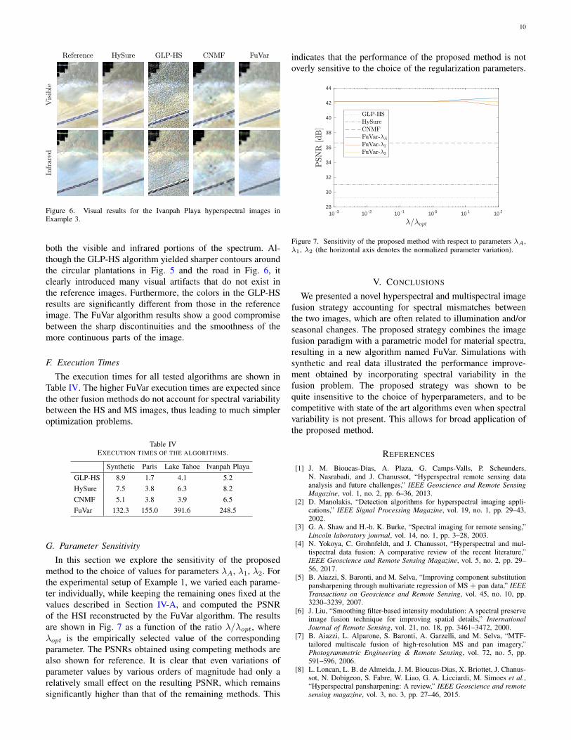
Figure 6. Visual results for the Ivanpah Playa hyperspectral images inExample 3.

both the visible and infrared portions of the spectrum. Al-though the GLP-HS algorithm yielded sharper contours aroundthe circular plantations in Fig. 5 and the road in Fig. 6, itclearly introduced many visual artifacts that do not exist inthe reference images. Furthermore, the colors in the GLP-HSresults are significantly different from those in the referenceimage. The FuVar algorithm results show a good compromisebetween the sharp discontinuities and the smoothness of themore continuous parts of the image.

F. Execution Times

The execution times for all tested algorithms are shown inTable IV. The higher FuVar execution times are expected sincethe other fusion methods do not account for spectral variabilitybetween the HS and MS images, thus leading to much simpleroptimization problems.

Table IVEXECUTION TIMES OF THE ALGORITHMS.

Synthetic Paris Lake Tahoe Ivanpah Playa

GLP-HS 8.9 1.7 4.1 5.2HySure 7.5 3.8 6.3 8.2CNMF 5.1 3.8 3.9 6.5FuVar 132.3 155.0 391.6 248.5

G. Parameter Sensitivity

In this section we explore the sensitivity of the proposedmethod to the choice of values for parameters λA, λ1, λ2. Forthe experimental setup of Example 1, we varied each parame-ter individually, while keeping the remaining ones fixed at thevalues described in Section IV-A, and computed the PSNRof the HSI reconstructed by the FuVar algorithm. The resultsare shown in Fig. 7 as a function of the ratio λ/λopt, whereλopt is the empirically selected value of the correspondingparameter. The PSNRs obtained using competing methods arealso shown for reference. It is clear that even variations ofparameter values by various orders of magnitude had only arelatively small effect on the resulting PSNR, which remainssignificantly higher than that of the remaining methods. This

indicates that the performance of the proposed method is notoverly sensitive to the choice of the regularization parameters.

10 -3 10 -2 10 -1 10 0 10 1 10 228

30

32

34

36

38

40

42

44

Figure 7. Sensitivity of the proposed method with respect to parameters λA,λ1, λ2 (the horizontal axis denotes the normalized parameter variation).

V. CONCLUSIONS

We presented a novel hyperspectral and multispectral imagefusion strategy accounting for spectral mismatches betweenthe two images, which are often related to illumination and/orseasonal changes. The proposed strategy combines the imagefusion paradigm with a parametric model for material spectra,resulting in a new algorithm named FuVar. Simulations withsynthetic and real data illustrated the performance improve-ment obtained by incorporating spectral variability in thefusion problem. The proposed strategy was shown to bequite insensitive to the choice of hyperparameters, and to becompetitive with state of the art algorithms even when spectralvariability is not present. This allows for broad application ofthe proposed method.

REFERENCES

[1] J. M. Bioucas-Dias, A. Plaza, G. Camps-Valls, P. Scheunders,N. Nasrabadi, and J. Chanussot, “Hyperspectral remote sensing dataanalysis and future challenges,” IEEE Geoscience and Remote SensingMagazine, vol. 1, no. 2, pp. 6–36, 2013.

[2] D. Manolakis, “Detection algorithms for hyperspectral imaging appli-cations,” IEEE Signal Processing Magazine, vol. 19, no. 1, pp. 29–43,2002.

[3] G. A. Shaw and H.-h. K. Burke, “Spectral imaging for remote sensing,”Lincoln laboratory journal, vol. 14, no. 1, pp. 3–28, 2003.

[4] N. Yokoya, C. Grohnfeldt, and J. Chanussot, “Hyperspectral and mul-tispectral data fusion: A comparative review of the recent literature,”IEEE Geoscience and Remote Sensing Magazine, vol. 5, no. 2, pp. 29–56, 2017.

[5] B. Aiazzi, S. Baronti, and M. Selva, “Improving component substitutionpansharpening through multivariate regression of MS + pan data,” IEEETransactions on Geoscience and Remote Sensing, vol. 45, no. 10, pp.3230–3239, 2007.

[6] J. Liu, “Smoothing filter-based intensity modulation: A spectral preserveimage fusion technique for improving spatial details,” InternationalJournal of Remote Sensing, vol. 21, no. 18, pp. 3461–3472, 2000.

[7] B. Aiazzi, L. Alparone, S. Baronti, A. Garzelli, and M. Selva, “MTF-tailored multiscale fusion of high-resolution MS and pan imagery,”Photogrammetric Engineering & Remote Sensing, vol. 72, no. 5, pp.591–596, 2006.

[8] L. Loncan, L. B. de Almeida, J. M. Bioucas-Dias, X. Briottet, J. Chanus-sot, N. Dobigeon, S. Fabre, W. Liao, G. A. Licciardi, M. Simoes et al.,“Hyperspectral pansharpening: A review,” IEEE Geoscience and remotesensing magazine, vol. 3, no. 3, pp. 27–46, 2015.

11

[9] N. Keshava and J. F. Mustard, “Spectral unmixing,” IEEE SignalProcessing Magazine, vol. 19, no. 1, pp. 44–57, 2002.

[10] T. Imbiriba, R. A. Borsoi, and J. C. M. Bermudez, “A low-ranktensor regularization strategy for hyperspectral unmixing,” in 2018 IEEEStatistical Signal Processing Workshop (SSP), 2018, pp. 373–377.

[11] R. A. Borsoi, T. Imbiriba, J. C. Moreira Bermudez, and C. Richard,“Tech Report: A Fast Multiscale Spatial Regularization for SparseHyperspectral Unmixing,” ArXiv e-prints, Dec. 2017.

[12] R. C. Hardie, M. T. Eismann, and G. L. Wilson, “MAP estimation forhyperspectral image resolution enhancement using an auxiliary sensor,”IEEE Transactions on Image Processing, vol. 13, no. 9, pp. 1174–1184,2004.

[13] Q. Wei, N. Dobigeon, and J.-Y. Tourneret, “Fast fusion of multi-bandimages based on solving a sylvester equation,” IEEE Transactions onImage Processing, vol. 24, no. 11, pp. 4109–4121, 2015.

[14] Q. Wei, J. Bioucas-Dias, N. Dobigeon, and J.-Y. Tourneret, “Hyperspec-tral and multispectral image fusion based on a sparse representation,”IEEE Transactions on Geoscience and Remote Sensing, vol. 53, no. 7,pp. 3658–3668, 2015.

[15] N. Akhtar, F. Shafait, and A. Mian, “Bayesian sparse representationfor hyperspectral image super resolution,” in Proceedings of the IEEEConference on Computer Vision and Pattern Recognition, 2015, pp.3631–3640.

[16] R. Kawakami, Y. Matsushita, J. Wright, M. Ben-Ezra, Y.-W. Tai, andK. Ikeuchi, “High-resolution hyperspectral imaging via matrix factoriza-tion,” in Computer Vision and Pattern Recognition (CVPR), 2011 IEEEConference on. IEEE, 2011, pp. 2329–2336.

[17] E. Wycoff, T.-H. Chan, K. Jia, W.-K. Ma, and Y. Ma, “A non-negativesparse promoting algorithm for high resolution hyperspectral imaging,”in Acoustics, Speech and Signal Processing (ICASSP), 2013 IEEEInternational Conference on. IEEE, 2013, pp. 1409–1413.

[18] M. Simões, J. Bioucas-Dias, L. B. Almeida, and J. Chanussot, “A convexformulation for hyperspectral image superresolution via subspace-basedregularization,” IEEE Transactions on Geoscience and Remote Sensing,vol. 53, no. 6, pp. 3373–3388, 2015.

[19] M. A. Veganzones, M. Simoes, G. Licciardi, N. Yokoya, J. M. Bioucas-Dias, and J. Chanussot, “Hyperspectral super-resolution of locally lowrank images from complementary multisource data,” IEEE Transactionson Image Processing, vol. 25, no. 1, pp. 274–288, 2016.

[20] N. Yokoya, T. Yairi, and A. Iwasaki, “Coupled nonnegative matrixfactorization unmixing for hyperspectral and multispectral data fusion,”IEEE Transactions on Geoscience and Remote Sensing, vol. 50, no. 2,pp. 528–537, 2012.

[21] C. Lanaras, E. Baltsavias, and K. Schindler, “Hyperspectral super-resolution by coupled spectral unmixing,” in Proceedings of the IEEEInternational Conference on Computer Vision, 2015, pp. 3586–3594.

[22] S. Li, R. Dian, L. Fang, and J. M. Bioucas-Dias, “Fusing hyperspectraland multispectral images via coupled sparse tensor factorization,” IEEETransactions on Image Processing, 2018.

[23] C. Kanatsoulis, X. Fu, N. Sidiropoulos, and W.-K. Ma, “Hyperspectralsuper-resolution via coupled tensor factorization: Identifiability andalgorithms,” in Acoustics, Speech and Signal Processing (ICASSP), 2018IEEE International Conference on. IEEE, 2018, pp. 3191–3195.

[24] A. Eckardt, J. Horack, F. Lehmann, D. Krutz, J. Drescher, M. Whorton,and M. Soutullo, “DESIS (dlr earth sensing imaging spectrometer forthe iss-muses platform),” in Geoscience and Remote Sensing Symposium(IGARSS), 2015 IEEE International. IEEE, 2015, pp. 1457–1459.

[25] H. Kaufmann, K. Segl, S. Chabrillat, S. Hofer, T. Stuffler, A. Mueller,R. Richter, G. Schreier, R. Haydn, and H. Bach, “EnMAP a hyperspec-tral sensor for environmental mapping and analysis,” in Geoscience andRemote Sensing Symposium, 2006. IGARSS 2006. IEEE InternationalConference on. IEEE, 2006, pp. 1617–1619.

[26] F. Gao, J. Masek, M. Schwaller, and F. Hall, “On the blending of thelandsat and MODIS surface reflectance: Predicting daily landsat surfacereflectance,” IEEE Transactions on Geoscience and Remote sensing,vol. 44, no. 8, pp. 2207–2218, 2006.

[27] D. P. Roy, J. Ju, P. Lewis, C. Schaaf, F. Gao, M. Hansen, andE. Lindquist, “Multi-temporal MODIS–landsat data fusion for relativeradiometric normalization, gap filling, and prediction of landsat data,”Remote Sensing of Environment, vol. 112, no. 6, pp. 3112–3130, 2008.

[28] T. Hilker, M. A. Wulder, N. C. Coops, N. Seitz, J. C. White, F. Gao,J. G. Masek, and G. Stenhouse, “Generation of dense time seriessynthetic landsat data through data blending with modis using a spatialand temporal adaptive reflectance fusion model,” Remote Sensing ofEnvironment, vol. 113, no. 9, pp. 1988–1999, 2009.

[29] T. Hilker, M. A. Wulder, N. C. Coops, J. Linke, G. McDermid, J. G.Masek, F. Gao, and J. C. White, “A new data fusion model for high

spatial-and temporal-resolution mapping of forest disturbance based onlandsat and modis,” Remote Sensing of Environment, vol. 113, no. 8, pp.1613–1627, 2009.

[30] I. V. Emelyanova, T. R. McVicar, T. G. Van Niel, L. T. Li, and A. I.van Dijk, “Assessing the accuracy of blending landsat–MODIS surfacereflectances in two landscapes with contrasting spatial and temporaldynamics: A framework for algorithm selection,” Remote Sensing ofEnvironment, vol. 133, pp. 193–209, 2013.

[31] A. Zare and K. C. Ho, “Endmember variability in hyperspectral anal-ysis: Addressing spectral variability during spectral unmixing,” SignalProcessing Magazine, IEEE, vol. 31, p. 95, January 2014.

[32] B. Somers, K. Cools, S. Delalieux, J. Stuckens, D. V. der Zande, W. W.Verstraeten, and P. Coppin, “Nonlinear hyperspectral mixture analysisfor tree cover estimates in orchards,” Remote Sensing of Environment,vol. 113, no. 6, pp. 1183–1193, February 2009.

[33] C. Lanaras, E. Baltsavias, and K. Schindler, “Hyperspectral super-resolution by coupled spectral unmixing,” in Proceedings of the IEEEInternational Conference on Computer Vision, 2015, pp. 3586–3594.

[34] L. Drumetz, M.-A. Veganzones, S. Henrot, R. Phlypo, J. Chanussot,and C. Jutten, “Blind hyperspectral unmixing using an extended linearmixing model to address spectral variability,” IEEE Transactions onImage Processing, vol. 25, no. 8, pp. 3890–3905, 2016.

[35] P.-A. Thouvenin, N. Dobigeon, and J.-Y. Tourneret, “Hyperspectralunmixing with spectral variability using a perturbed linear mixingmodel,” IEEE Transactions on Signal Processing, vol. 64, no. 2, pp.525–538, 2016.

[36] T. Imbiriba, R. A. Borsoi, and J. C. M. Bermudez, “Generalized linearmixing model accounting for endmember variability,” in Acoustics,Speech and Signal Processing (ICASSP), 2018 IEEE InternationalConference on. IEEE, 2018, pp. 1862–1866.

[37] M.-D. Iordache, J. M. Bioucas-Dias, and A. Plaza, “Total variationspatial regularization for sparse hyperspectral unmixing,” IEEE Transac-tions on Geoscience and Remote Sensing, vol. 50, no. 11, pp. 4484–4502,2012.

[38] S. Boyd, N. Parikh, E. Chu, B. Peleato, and J. Eckstein, “Distributedoptimization and statistical learning via the alternating direction methodof multipliers,” Foundations and Trends R© in Machine Learning, vol. 3,no. 1, pp. 1–122, 2011.

[39] R. E. Roger and J. F. Arnold, “Reliably estimating the noise in AVIRIShyperspectral images,” International Journal of Remote Sensing, vol. 17,no. 10, pp. 1951–1962, 1996.

[40] J. M. Nascimento and J. M. Dias, “Vertex component analysis: Afast algorithm to unmix hyperspectral data,” IEEE transactions onGeoscience and Remote Sensing, vol. 43, no. 4, pp. 898–910, 2005.

[41] L. Wald, “Quality of high resolution synthesised images: Is there asimple criterion?” in Third conference" Fusion of Earth data: merg-ing point measurements, raster maps and remotely sensed images".SEE/URISCA, 2000, pp. 99–103.

[42] Z. Wang and A. C. Bovik, “A universal image quality index,” IEEEsignal processing letters, vol. 9, no. 3, pp. 81–84, 2002.