Sunk Costs of R&D, Trade and Productivity:

the moulds industry case�

Carlos Daniel Santosy

University of Alicante and Centre for Economic Performance

September 27, 2010

Abstract

Evidence suggests that trade improves industry productivity via (i) selection of the best

�rms and (ii) within �rm productivity growth. While the selection e¤ect has been well ex-

plained by the literature, the productivity growth is not accounted for in standard models.

Trade liberalization creates economies of scale in the R&D process that can explain the

observed growth. I estimate a model of industry dynamics with endogenous productivity,

capital accumulation and aggregate uncertainty. I use data from the Portuguese moulds

industry which experienced an exogenous trade shock in 1993 (establishment of the Com-

mon Market) and a signi�cant increase in foreign demand afterwards. Firms exploited the

increase in demand from other European countries to increase R&D spending. The �nal

results con�rm the trade-induced innovation e¤ect.

Keywords: Industry Dynamics, Innovation, Markov Equilibrium, Moulds Industry,

R&D, Structural Estimation, Sunk Costs, Trade

JEL Classi�cation: C61, D92, L11, L22, O31

1 Introduction

I investigate the e¤ects of trade on productivity in the presence of sunk costs for Research and

Development. The mechanism works as follows. When trade barriers are reduced, �rms have

access to external markets. This increase in market size gives �rms enough scale to devote

�Acknowledgments: I would like to thank John Van Reenen and Philipp Schmidt-Dengler for all theirguidance and support. I would also like to thank Jérôme Adda, Stephen Bond, Ulrich Doraszelski, Cristian Huse,Sorin Krammer, Vadym Lepetyuk, Mark Roberts, Bernard Salanié, Adam Sanjurjo and Gabriel Weintraub andparticipants at several meetings and conferences for very useful comments and suggestions. This manuscript ispart of my Ph.D. dissertation at The London School of Economics and was previously named "Recovering theSunk Costs of R&D: the moulds industry case". Research supported by the Portuguese Science and TechnologyFoundation grant SFRH/BD/12092/2003.

yUniversity of Alicante, Campus San Vicente, 03080 Alicante, Spain; csantos@ua.es

1

more resources towards R&D and pay the sunk costs. R&D generates future innovations and

productivity growth - further increasing the gains from trade.1 I estimate the sunk costs using

data from the Portuguese moulds industry after the country joined the EU in 1986 and the

Common Market came in place in 1993. I then illustrate the trade-induced innovation e¤ect

by exogenously varying market size and calculating the new stationary equilibrium (using the

estimated structural parameters). If market size is reduced to the level of 1994, the model

predicts a reduction in R&D performance, average productivity, capital stock and number of

�rms - in line with the evidence. To my knowledge this paper is the �rst to propose and

estimate a dynamic game with many players. The estimation method used can be applied to

other studies with microdata on industry dynamics, trade or macroeconomics.

Recent advances in the trade literature were quite successful in explaining the important

role of �rm level productivity and technology in international trade (Eaton and Kortum (2002),

Melitz (2003), Bernard et al. (2003)). However, these models consider productivity to be

exogenous and are not able to reconcile with some of the empirical evidence. In particular, the

models cannot account for three of the stylized facts: the within �rm productivity growth after

trade liberalization (Pavnick (2002) and Bernard et al. (2006)), the important role of �rm size

as a determinant of export behavior, even after conditioning on productivity, and the increase in

average sales per �rm with market size (Eaton, Kortum and Kramarz (2008)).2 To rationalize

the evidence I introduce endogenous choice of technology and size (physical capital) by modeling

the adjustment costs for investment and sunk costs for R&D. By so doing, I extend the analysis

of the recent trade literature along the technology dimension while abstracting from the role

of geography. Economic integration reduces uncertainty. Adjustment costs for capital and

aggregate uncertainty are used to generate market size e¤ects. Physical capital and aggregate

uncertainty create an option value for investment that generates the observed non-neutrality to

market size. Further, I show that this non-neutrality leads to an increase in average size and

thus a consequent increase in R&D.3 Trade then provides the same opportunities to an open

economy as would an increase in country size to a closed economy.

There is also a relatively large literature documenting �rms�joint decisions of export and

innovation. For example, Aw, Roberts and Xu (2009) develop a single agent framework in

which �rms decide whether or not to enter the export market and whether or not to invest

in R&D. They �nd an interaction between R&D and export status due to the tendency of

high productivity plants to self select into exporting and R&D. While I do not model export

1Pavcnik (2002) estimates the trade gains for the Chilean industry and De Loecker (2007) for the Belgiantextile industry.

2The industrial organization literature has for a long time recognized that market structure depends onmarket size. This dependence can be due to the competition e¤ects induced in larger markets (Bresnahan andReiss (1991)). Melitz and Ottaviano (2008) introduce endogenous markups in a trade model to rationalizemarket size e¤ects.

3Sutton (1991, 1998) explains how in the presence of sunk costs, market structure does not become fragmentedwith increases in market size; on average, �rms become larger as market size increases.

2

decisions separately from internal sales, I would expect similar size e¤ects on export decisions

and innovation. Finally, there is some evidence for �learning-by-exporting�with productivity

improvements following export market participation (see the survey in Lopez (2005)). It is

not clear how we could disentangle the e¤ects of R&D from pure learning. In a certain way,

learning can be regarded as a form of R&D if it involves dedicated e¤ort. In this case, learning

and R&D are similar and both lead to higher productivity.

In setting up the model, I bring together the literature of endogenous innovation and in-

vestment. It is by now commonly accepted that in most industries innovating �rms are more

productive, larger and less likely to exit. Klette and Kortum (2004) propose an elegant general

equilibrium model of innovation which can explain these stylized facts about R&D and indus-

try dynamics. I build on their model and extend it to allow for physical capital investment.

Such extension provides a better �t for the empirical analysis but comes at the cost of loosing

analytical solutions.4

The investment literature has considered decisions in which investment is lumpy. Authors

have attempted to explain this investment lumpiness with non-convex adjustment costs such as

irreversibilities and �xed costs (see Cooper and Haltiwanger (2006)). Besides providing a good

�t to the microevidence, such costs can rationalize the large persistence in size, as well as the

investment reaction to risk and volatility.

The model is speci�ed as to capture some of the empirical facts. Size is a considerable

determinant of R&D decisions, and innovations resulting from R&D expenditures later translate

into productivity increases.5 The decision to export depends on both �rm size and productivity.

For example, capital stock and productivity explain 15% and 8% of the variation in exporting

behavior. Finally, a high persistence in capital and productivity motivates the use of a dynamic

model.

My model is similar in spirit to the industry equilibrium models of Hopenhayn (1992) and

Ericson and Pakes (1995). I introduce incomplete information and assume that individual

players do not observe the state or actions of their competitors. Players�strategies and beliefs

are Markovian and depend on payo¤ relevant states. This assumption allows us to break the

"curse of dimensionality" and solve the model with a large number of players. Estimation

is done in three steps using the method developed by Bajari, Benkard and Levin (2008),

henceforth BBL. In the �rst step productivity is recovered using production function estimation

methods. In the second step, payo¤, policy and transition functions are estimated. Finally, in

4 I use a variation of their model. Similarly to Melitz (2003) I use productivity as the measure of knowledgewhereas Klette and Kortum (2004) use the number of products. Using the number of products together withassuming a monopoly market for each product, has some bene�ts in their case since it allows the return functionto be linear in the knowledge stock. Linearity simpli�es the dynamic problem with a value function that isalso linear in knowledge stock and can be characterized analytically. A second di¤erence from their work is theintroduction of discrete innovation decisions.

5Productivity here is broadly de�ned as either total factor productivity or price-cost margins.

3

the third step I search for parameters to rationalize the estimated policy functions as optimal.

The available data determines the parametrization and the structural elements that can be

identi�ed. Although the model is quite general, here I adopt a speci�c parametrization for

empirical purposes. In the last section, I evaluate the impact of changes in (i) market size, (ii)

sunk costs of R&D, and (iii) entry costs on investment, productivity and market structure. The

results con�rm that average �rm size and R&D are lower with either a smaller market size or

larger sunk costs.

One issue I do not address is the existence of persistent unobserved heterogeneity. The

�rst reason I avoid this problem is that estimated productivity captures part of the unobserved

heterogeneity. The second reason is that persistence in marginal costs or bene�ts for investment

or R&D is a di¢ cult topic to address in the estimation of structural models. Because the models

used here are nonlinear, it seems that dealing with persistent unobserved heterogeneity can only

be done with su¢ ciently large time series.

2 The moulds industry

The Portuguese moulds industry is an interesting success case. The ability to develop itself even

in the absence of a national market and the fact that most of the production has always been

exported illustrates the importance of foreign markets. Between 1994 and 2003 the growth in

exports was mainly to other European countries in detriment of the US, traditionally the larger

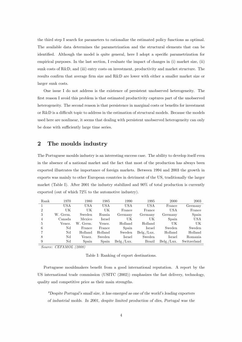
market (Table I). After 2001 the industry stabilized and 90% of total production is currently

exported (out of which 72% to the automotive industry).

Rank 1970 1980 1985 1990 1995 2000 20031 USA USA USA USA USA France Germany2 UK UK UK France France USA France3 W. Germ. Sweden Russia Germany Germany Germany Spain4 Canada Mexico Israel UK UK Spain USA5 Venez. W. Germ. Venez. Holland Holland UK UK6 Nd France France Spain Israel Sweden Sweden7 Nd Holland Holland Sweden Belg./Lux. Holland Holland8 Nd Venez. Sweden Israel Sweden Israel Romania9 Nd Spain Spain Belg./Lux. Brazil Belg./Lux. Switzerland

Source: CEFAMOL (2008)

Table I: Ranking of export destinations.

Portuguese mouldmakers bene�t from a good international reputation. A report by the

US international trade commission (USITC (2002)) emphasizes the fast delivery, technology,

quality and competitive price as their main strengths.

"Despite Portugal�s small size, it has emerged as one of the world�s leading exporters

of industrial molds. In 2001, despite limited production of dies, Portugal was the

4

eighth largest producer of dies and molds in the world and it exports to more than

70 countries. The Portuguese TDM (Tools, Dies and Moulds) industry�s success in

exporting, and in adoption of the latest computer technologies, has occurred despite

the fact that Portugal has a small industrial base on which the TDM industry can

depend. Since joining the EU in 1986, Portugal has focused on serving customers

in the common market." (USITC (2002)

Entering the European Economic Community in 1986 and the establishment of the Common

European Market in 1993 were two important factors driving the observed growth. With such

events, �rms were able to reach important European producers and later increase R&D and

innovation. Beira et al. (2003) and IAPMEI (2006) document how the close collaboration with

car makers constituted a strong push for the development of new processes and products, nor-

mally in the form of research projects. These research projects are typically implemented over

a given time frame and have well de�ned targets and objectives. Projects have to be completed,

and upon completion the gains become permanent. This type of project-based R&D motivates

the sunk cost speci�cation. An alternative current expenditures, or �xed costs, approach would

be better suited for industries where instead of projects, R&D is performed continuously (for

example the chemical or pharmaceutical industries). Such �xed cost speci�cation would not

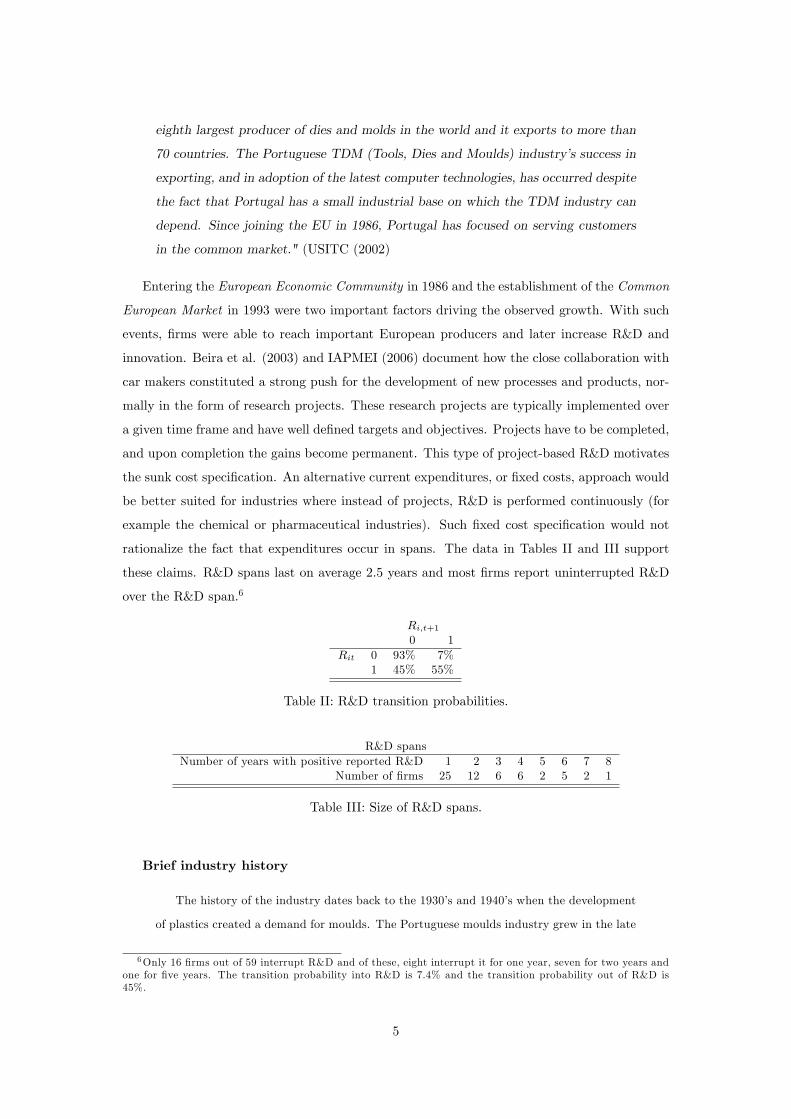
rationalize the fact that expenditures occur in spans. The data in Tables II and III support

these claims. R&D spans last on average 2.5 years and most �rms report uninterrupted R&D

over the R&D span.6

Ri;t+10 1

Rit 0 93% 7%1 45% 55%

Table II: R&D transition probabilities.

R&D spansNumber of years with positive reported R&D 1 2 3 4 5 6 7 8

Number of �rms 25 12 6 6 2 5 2 1

Table III: Size of R&D spans.

Brief industry history

The history of the industry dates back to the 1930�s and 1940�s when the development

of plastics created a demand for moulds. The Portuguese moulds industry grew in the late

6Only 16 �rms out of 59 interrupt R&D and of these, eight interrupt it for one year, seven for two years andone for �ve years. The transition probability into R&D is 7.4% and the transition probability out of R&D is45%.

5

1950�s as a major supplier of moulds for the glass (where it inherited some of its expertise)

but mainly for the toy industry. In the late 1980�s the production started shifting from

toy manufacturing towards the growing industries of automobiles and packaging. During

the 1990�s the largest markets shifted from the US to France, Germany and Spain (Table

I, IAPMEI (2006)).

The industry underwent several changes with the introduction of new technologies

(e.g. CAD, CAM, Complex process, In-mould Assembling) and an increasing importance

of innovation and R&D. For example, the technology used in computer operated machines

radically changed from the 1980�s to the 1990�s. State of the art machinery allows �exibility

at a low cost. It also allows a close collaboration with the client in the design phase. Design

teams can work closely with the engineers and produce 3D virtual versions of the mould

which is produced in the �nal phase. Controlling the technology was a major requirement

for car-manufacturers and an advantage of Portuguese producers.

2.1 Sample description

The sample is part of the Central de Balanços compiled by Portuguese Central Bank for the

period between 1994 to 2003. It contains �nancial information (balance sheet and P&L) together

with other characterization variables: number of workers, total exports, R&D, founding year

and current status (e.g. operating, bankrupt, etc). The �ve-digit industry code (NACE, revision

1.1) is 29563. Industry aggregate variables for sales, number of �rms, employment and value

added are collected from the Portuguese National Statistics O¢ ce (INE (2007)) and industry

prices from IAPMEI (2006). The Appendix provides a description of the sample and variable

construction.

There are 1,290 observations for 231 �rms, out of which 265 observations with positive R&D

corresponding to 59 �rms and 49 R&D start-ups (Table A.II). The average �rm in the sample

sells goods worth 1.5 million Euros and employs 32 workers with an average labor productivity

of 20,381 Euros. The industry is populated by many small and medium �rms with no market

leaders. R&D �rms are three times larger, 20% more productive and export more (Table A.I).

Stationarity Over the period, real sales grew at an average 8.9% per year and labor

productivity at 5.7% (Tables A.III and A.I) raising some concerns over non-stationarity. Growth

in average sales is mostly concentrated in the 1994 to 1998 period with a stabilization after 1998

occurring due to the increase in the number of �rms (Figure A.1). The growth and stabilization

are consistent with a structural shock occurring somewhere before 1994 with the observed years

of 1994 to 1998 being a period of transitional dynamics. This structural shock was the European

economic integration that culminated with the establishment of the Common Market in 1993.

Thus, I will abstract from any non-stationarity concerns.

6

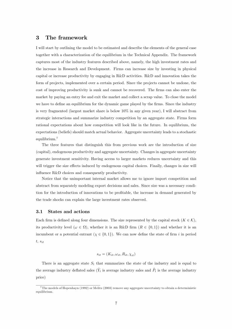
3 The framework

I will start by outlining the model to be estimated and describe the elements of the general case

together with a characterization of the equilibrium in the Technical Appendix. The framework

captures most of the industry features described above, namely, the high investment rates and

the increase in Research and Development. Firms can increase size by investing in physical

capital or increase productivity by engaging in R&D activities. R&D and innovation takes the

form of projects, implemented over a certain period. Since the projects cannot be undone, the

cost of improving productivity is sunk and cannot be recovered. The �rms can also enter the

market by paying an entry fee and exit the market and collect a scrap value. To close the model

we have to de�ne an equilibrium for the dynamic game played by the �rms. Since the industry

is very fragmented (largest market share is below 10% in any given year), I will abstract from

strategic interactions and summarize industry competition by an aggregate state. Firms form

rational expectations about how competition will look like in the future. In equilibrium, the

expectations (beliefs) should match actual behavior. Aggregate uncertainty leads to a stochastic

equilibrium.7

The three features that distinguish this from previous work are the introduction of size

(capital), endogenous productivity and aggregate uncertainty. Changes in aggregate uncertainty

generate investment sensitivity. Having access to larger markets reduces uncertainty and this

will trigger the size e¤ects induced by endogenous capital choices. Finally, changes in size will

in�uence R&D choices and consequently productivity.

Notice that the unimportant internal market allows me to ignore import competition and

abstract from separately modeling export decisions and sales. Since size was a necessary condi-

tion for the introduction of innovations to be pro�table, the increase in demand generated by

the trade shocks can explain the large investment rates observed.

3.1 States and actions

Each �rm is de�ned along four dimensions. The size represented by the capital stock (K 2 K),

its productivity level (! 2 ), whether it is an R&D �rm (R 2 f0; 1g) and whether it is an

incumbent or a potential entrant (� 2 f0; 1g). We can now de�ne the state of �rm i in period

t, sit

sit = (Kit; !it; Rit; �it)

There is an aggregate state St that summarizes the state of the industry and is equal to

the average industry de�ated sales ( ~Yt is average industry sales and ~Pt is the average industry

price)

7The models of Hopenhayn (1992) or Melitz (2003) remove any aggregate uncertainty to obtain a deterministicequilibrium.

7

St =~Yt~Pt

To �t the model statistically I specify unobserved heterogeneity. Payo¤ shocks are privately

observed by the �rm, unobserved by the econometrician and include shocks to investment costs

"Iit , to the sunk cost "RDit , to the scrap value "

scrapit , and to pro�ts "�it. The distribution

of these shocks is nonparametrically unidenti�ed (see section 4.4). The shocks also have to

satisfy conditional independence (Rust (1994)). Thus, I will assume the vector of payo¤ shocks

"it = ("I ; "RD; "entry; "scrap; "�it) are draw from a distribution, F (").

Firms�available choices are the investment level (I 2 R+) which will add to the current

capital stock and generate growth, and R&D (R 2 f0; 1g) which will lead to productivity

improvements. Firms can also decide to enter or exit (� 2 f0; 1g) from the industry. Summarize

these choices in the vector of actions ait

ait = (Ii;t+1; Ri;t+1; �i;t+1)

For convenience I will sometimes use the short notations for the vector of states and actions

(sit; ait) and in other occasions I use the actual states and actions.

3.2 State transition

Individual states evolve over time with a controlled �rst order Markov transition. Most natu-

rally, the evolution of capital is deterministic while productivity evolves stochastically.

Productivity R&D �rms have better prospects for their productivity than non-R&D

�rms (in a probabilistic sense). Unless �rm level prices are observed, we cannot separate "true"

productivity from price margins. In the absence of observed �rm level prices, we have to use a

broad de�nition for productivity.

The internal source of uncertainty distinguishes R&D investment from other decisions like

capital investment, labor hiring, entry and exit which have deterministic outcomes and where

the sources of uncertainty are external to the company (e.g. due to the environment, competi-

tion, demand, etc.). Productivity follows a controlled �rst order Markov process.

!i;t+1 = E(!i;t+1j!it; Rit) + �!i;t+1 (1)

= P :;!(!it; Rit) + �!i;t+1

where v!it is independently and identically distributed across �rms and time and P:;!(:) is a

parametric function used to approximate the conditional expectation function. The transition

for individual productivity is estimated separately for R&D and non-R&D �rms and several

functional forms for P :;!(:) will be reported, including polynomial function of order n.

8

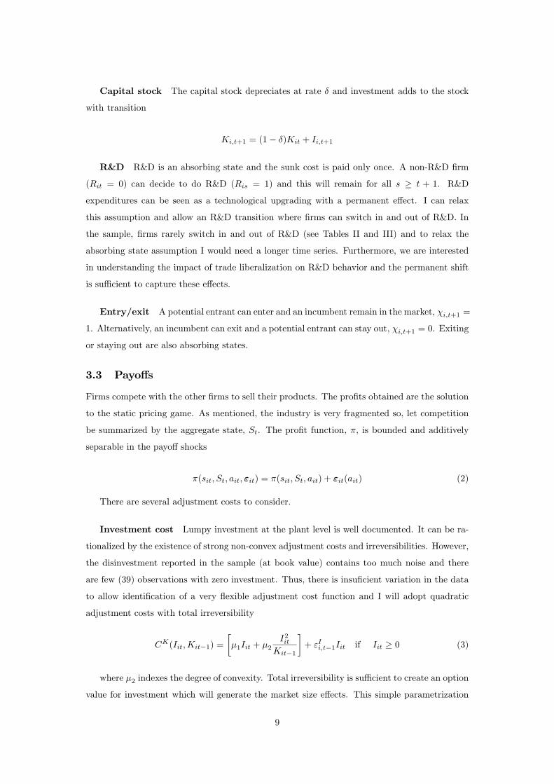
Capital stock The capital stock depreciates at rate � and investment adds to the stock

with transition

Ki;t+1 = (1� �)Kit + Ii;t+1

R&D R&D is an absorbing state and the sunk cost is paid only once. A non-R&D �rm

(Rit = 0) can decide to do R&D (Ris = 1) and this will remain for all s � t + 1. R&D

expenditures can be seen as a technological upgrading with a permanent e¤ect. I can relax

this assumption and allow an R&D transition where �rms can switch in and out of R&D. In

the sample, �rms rarely switch in and out of R&D (see Tables II and III) and to relax the

absorbing state assumption I would need a longer time series. Furthermore, we are interested

in understanding the impact of trade liberalization on R&D behavior and the permanent shift

is su¢ cient to capture these e¤ects.

Entry/exit A potential entrant can enter and an incumbent remain in the market, �i;t+1 =

1. Alternatively, an incumbent can exit and a potential entrant can stay out, �i;t+1 = 0. Exiting

or staying out are also absorbing states.

3.3 Payo¤s

Firms compete with the other �rms to sell their products. The pro�ts obtained are the solution

to the static pricing game. As mentioned, the industry is very fragmented so, let competition

be summarized by the aggregate state, St. The pro�t function, �, is bounded and additively

separable in the payo¤ shocks

�(sit; St; ait; "it) = �(sit; St; ait) + "it(ait) (2)

There are several adjustment costs to consider.

Investment cost Lumpy investment at the plant level is well documented. It can be ra-

tionalized by the existence of strong non-convex adjustment costs and irreversibilities. However,

the disinvestment reported in the sample (at book value) contains too much noise and there

are few (39) observations with zero investment. Thus, there is insu�cient variation in the data

to allow identi�cation of a very �exible adjustment cost function and I will adopt quadratic

adjustment costs with total irreversibility

CK(Iit;Kit�1) =

��1Iit + �2

I2itKit�1

�+ "Ii;t�1Iit if Iit � 0 (3)

where �2 indexes the degree of convexity. Total irreversibility is su¢ cient to create an option

value for investment which will generate the market size e¤ects. This simple parametrization

9

still captures the important investment features: option value of investment and periods of

inaction. I also report estimates for the model where the quadratic term is set to zero and the

results show that the estimates of the remaining parameters are not a¤ected. A more general

form for the investment function is possible at the cost of increasing the number of parameters

to estimate.

R&D costs R&D decisions take the form of projects implemented over a given period -

technological upgrading, catchup innovation or introduction of new technologies. If the whole

project is not implemented the returns are likely to be small while they become permanent

upon completion. Sunk costs are a good �rst order approximation to the underlying R&D cost

structure. We can write them as �+ "RDit where � is the average sunk cost and "RDit is a private

cost shock. Not modeling current expenditures (variable or �xed costs) allows me to avoid

considering an extra policy function. As mentioned above, the evidence supports a sunk cost

speci�cation.8

Entry cost Potential entrants are short lived and cannot delay entry. Upon entry they

must pay a (privately observed) sunk entry fee of E+ "entryit to get a productivity/capital draw

from the distribution pE(!t+1;Kt+1j�t = 0). Since entry e¤ects are captured in the equilibrium

transition for the aggregate state, it is not necessary to model entry for the estimation. When

the equilibrium is calculated (as in the analysis of counterfactuals), the entry process will be

explicitly modeled.

Exit value Every period the �rm has the option of exiting the industry and receive a

scrap value of e + "scrapit . Changes to how exit is modeled have negligible e¤ects to the value

function and estimates of investment and sunk costs. Furthermore, the estimates for the exit

value are likely to be imprecise since there is little variation in observed exit.

Payo¤function Let � = (�1; �2; �; e) be the vector of cost parameters. Using the speci�ed

cost structure the per period return function of an incumbent is

�(!it;Kit; Rit; St; Ri;t+1; �i;t+1; Ii;t+1; "it;�; �) = (4)

= ~�(!it;Kit; St; �; "�) + "�it � �1Ii;t+1 � �2

I2i;t+1Kit

� "IitIi;t+1

�(�+ "RDit )(Ri;t+1 �Rit)Ri;t+1 + (1� �i;t+1)(e+ "scrapit )

8 In principle, sunk, �xed and variable costs are identi�able. The sunk costs would be identi�ed o¤ the �rsttime it was decided to do R&D, �xed costs would be identi�ed o¤ the switches in and out of R&D and �nallythe variable costs would be identi�ed o¤ the variations in observed R&D expenditures. In practice, this canonly be achieved if there is su¢ cient variation in the R&D data and a long time series.

10

Where ~�(:) is the gross pro�t function (gross of adjustment costs) and the payo¤ shocks

enter additively (Rust (1994)). The two aggregate variables are market size ( ~Y ) which evolves

exogenously and average industry price ( ~P ) which is determined endogenously.9

There are two options to specify the gross pro�t function, ~�(:). First we could parametrize

demand and the production function and write the reduced form sales as the solution to the

static pricing game. Examples that are consistent with the aggregate state speci�cation are

monopolistic competition or symmetric Cournot competition. Alternatively, if gross pro�ts are

observed, the pro�t function can be left unspeci�ed and estimated directly. The second route

is followed here. Reported cash �ows are used to estimate the pro�t function. Since cash �ows

can take negative values, I allow for �xed production costs

~�(!it;Kit; Rit; St; �) = �0e�1!itK�2

it S�3t + �4 + �5Kit + �6Rit (5)

where the vector of parameters, � = (�0; �1; �2; �3; �4; �5; �6) are estimated by nonlinear

least squares.

3.4 Value function

We can �nally write down the dynamic problem faced by an individual �rm. Players choose

actions to maximize the discounted sum of pro�ts

V (sit; St) = maxfaisg1s=t

Et

1Xs=t

�s�t�(sis; Ss; ais; "is)

= maxait

�(sit; St; ait; "it) + �Eaitt V (si;t+1; St+1)

where the expected continuation value is integrated over the possible values of the state

variables conditional on the current state and actions

Eaitt V (si;t+1; St+1) =

Zsi;t+1

ZSt+1

Vi;t+1p(ait; sit; si;t+1)q(sit; St; St+1)dsi;t+1dSt+1

the transition p(ait; sit; si;t+1) is the probability of reaching state si;t+1 from state sit when

action ait is chosen, and the function q(sit; St; St+1) is the probability of reaching state St+1

from state (sit; St). The individual transition (p(:)) is a primitive of the model assumed known

to all players, whereas the industry state transition (q(:)) represents the beliefs about the

evolution of the industry state.

9 Individual prices are determined in the static pricing game. Individual pricing strategies map individualstates into the price space (P �i = P (!i;Ki; ~P ; ~Y )). The aggregate state then puts all individual prices together

St =~Yt

~Pt(!;K;R; ~Y ).

11

Equilibrium In equilibrium, beliefs q(sit; St; St+1) are consistent with optimal behavior

(see the Technical Appendix) . The (stochastic) equilibrium transition for the aggregate state

is q�(sit; St; St+1).

4 The estimation procedure

The estimation is processed in three steps. In the �rst step, I estimate unobserved productivity

using several alternatives. In the second step I estimate the parameters, �, of pro�t function

(~�(!it;Kit; Rit; St; �)), the �rm-level and industry-level state transitions, (p(!i;t+1j!it; Rit; �it)

and q(St; St+1)) and the equilibrium policy functions for investment (I(!it;Kit; Rit; St)), R&D

(R(!it;Kit; Rit; St)) and exit (�(!it;Kit; Rit; St)).10 Finally, in the third step the dynamic

parameters (�1; �2; �; e) are recovered using the equilibrium conditions. Since the model has

no analytical solution, I use computational methods.

4.1 Step 1: Productivity

Total factor productivity is an unobserved state variable that can be estimated as the residual

from a production function.11 To estimate the production function I use the method proposed

by De Loecker (2007) that can be used in situations where revenues are observed instead of

quantities and there is imperfect competition (see also Klette and Griliches (1995)). The method

was developed for single agent models and I propose a slight extension that can be applied to

equilibrium models. The di¤erence in equilibrium models is that the input demand function

depends on the industry state, more precisely, the aggregate industry state (see Appendix for

a discussion A.2).12

4.2 Step 2: Policies and transitions

4.2.1 Policies

The policy functions are estimated with the observations for the state variables and actions. The

optimal solution to the dynamic problem faced by an individual �rm is the following investment

function

Ii;t+1Kit

=1

2�2

��@E(V (si;t+1; St+1jsit; St))

@Ii;t+1� �1

�� 1

2�2"Iit

which I estimate separately for R&D and non-R&D �rms using a �exible polynomial

10Assuming players own e¤ect on the aggregate state is negligible we can write q(sit; St; St+1) = q(St; St+1).This is the case when players are in�nitesimal.11Ackerberg et al. (2007) provide an excellent survey of the literature for estimating production functions.12There is also the selection problem resulting from exit of less productive �rms from the sample. Since the

number of exits observed in the data is very small, the correction for selection is negligible.

12

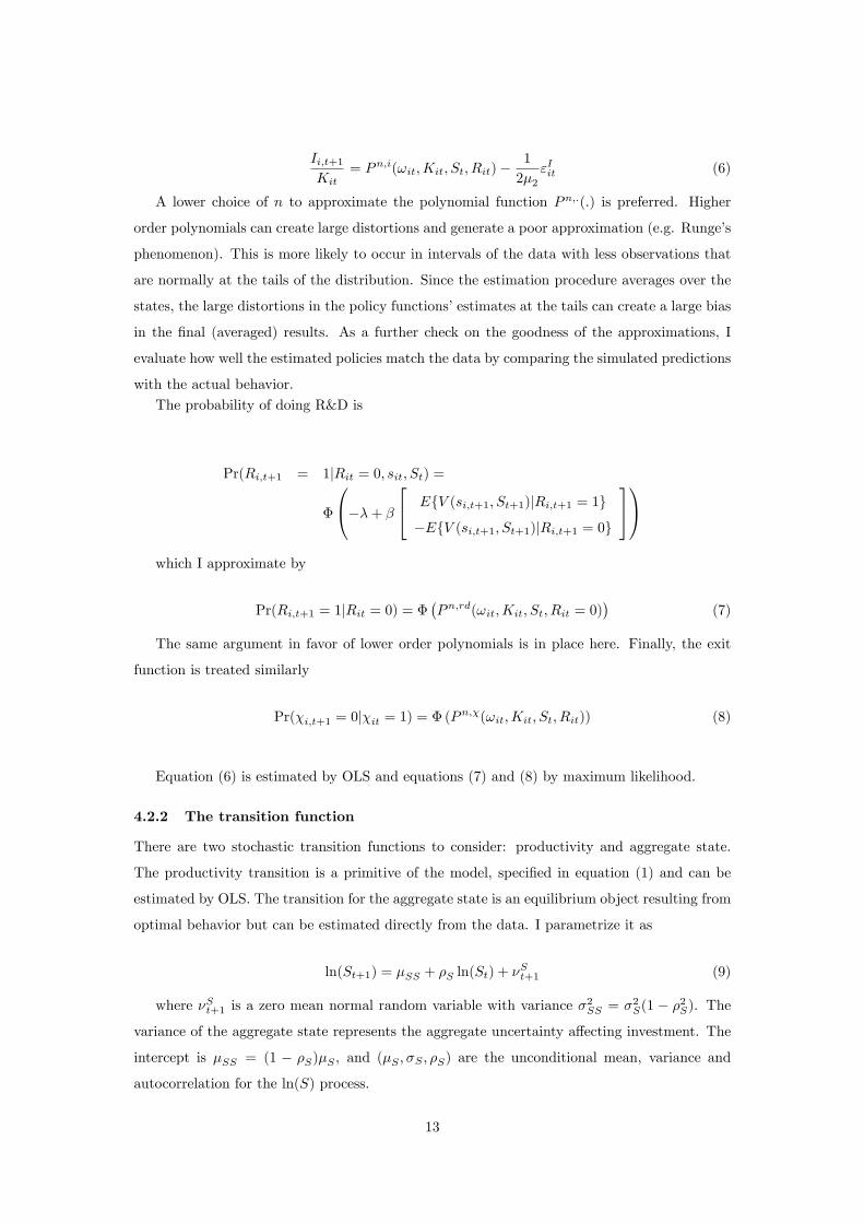
Ii;t+1Kit

= Pn;i(!it;Kit; St; Rit)�1

2�2"Iit (6)

A lower choice of n to approximate the polynomial function Pn;:(:) is preferred. Higher

order polynomials can create large distortions and generate a poor approximation (e.g. Runge�s

phenomenon). This is more likely to occur in intervals of the data with less observations that

are normally at the tails of the distribution. Since the estimation procedure averages over the

states, the large distortions in the policy functions�estimates at the tails can create a large bias

in the �nal (averaged) results. As a further check on the goodness of the approximations, I

evaluate how well the estimated policies match the data by comparing the simulated predictions

with the actual behavior.The probability of doing R&D is

Pr(Ri;t+1 = 1jRit = 0; sit; St) =

�

0@��+ �24 EfV (si;t+1; St+1)jRi;t+1 = 1g

�EfV (si;t+1; St+1)jRi;t+1 = 0g

351Awhich I approximate by

Pr(Ri;t+1 = 1jRit = 0) = ��Pn;rd(!it;Kit; St; Rit = 0)

�(7)

The same argument in favor of lower order polynomials is in place here. Finally, the exit

function is treated similarly

Pr(�i;t+1 = 0j�it = 1) = � (Pn;�(!it;Kit; St; Rit)) (8)

Equation (6) is estimated by OLS and equations (7) and (8) by maximum likelihood.

4.2.2 The transition function

There are two stochastic transition functions to consider: productivity and aggregate state.

The productivity transition is a primitive of the model, speci�ed in equation (1) and can be

estimated by OLS. The transition for the aggregate state is an equilibrium object resulting from

optimal behavior but can be estimated directly from the data. I parametrize it as

ln(St+1) = �SS + �S ln(St) + �St+1 (9)

where �St+1 is a zero mean normal random variable with variance �2SS = �2S(1 � �2S). The

variance of the aggregate state represents the aggregate uncertainty a¤ecting investment. The

intercept is �SS = (1 � �S)�S , and (�S ; �S ; �S) are the unconditional mean, variance and

autocorrelation for the ln(S) process.

13

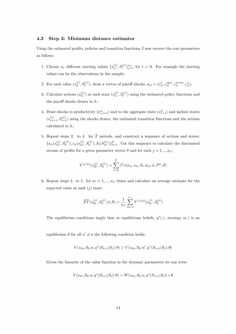
4.3 Step 3: Minimum distance estimator

Using the estimated pro�ts, policies and transition functions, I now recover the cost parameters

as follows:

1. Choose ns di¤erent starting values fs(j)it ; S(j)t gnSj=1 for t = 0. For example the starting

values can be the observations in the sample;

2. For each value (s(j)it ; S(j)t ), draw a vector of payo¤ shocks, "it = ("Iit; "

RDit ; "

scrapit ; "�it).

3. Calculate actions (a(j)it ) at each state (s(j)it ; S

(j)t ) using the estimated policy functions and

the payo¤ shocks drawn in 2.;

4. Draw shocks to productivity (�!i;t+1) and to the aggregate state (�St+1) and update states

(s(j)i;t+1; S

(j)t+1) using the shocks drawn, the estimated transition functions and the actions

calculated in 3.;

5. Repeat steps 2. to 4. for �T periods, and construct a sequence of actions and states:

fait(s(j)i0 ; S(j)0 ); sit(s

(j)i0 ; S

(j)0 ); St(S

(j)i0 )g

�Tt=1. Use this sequence to calculate the discounted

stream of pro�ts for a given parameter vector � and for each j = 1; ::; ns:

V (j;m)(s(j)i0 ; S

(j)0 ) =

�TXt=0

�t�(ait; sit; St; "it; �; Pn; �)

6. Repeat steps 2. to 5. for m = 1; :::; nJ times and calculate an average estimate for the

expected value at each (j) state:

dEV (s(j)i0 ; S(j)0 ; ~�; �) =1

nJ

nJXm=1

V (j;m)(s(j)i0 ; S

(j)0 )

The equilibrium conditions imply that at equilibrium beliefs, q�(:), strategy a(:) is an

equilibrium if for all a0 6= a the following condition holds:

V (si0; S0; a; q�(St+1jSt); �) � V (si0; S0; a0; q�(St+1jSt); �)

Given the linearity of the value function in the dynamic parameters we can write

V (si0; S0; a; q�(St+1jSt); �) =W (si0; S0; a; q�(St+1jSt)) � �

14

where � = [1; �1; �2; �; e], W (si0; S0; a; q�(St+1jSt)) = Eajsi0;S0

P1s=0 �

swis and wis =�e�(sis; Ss;�); Iis; I2is;1(Ris+1 = 1; Ris = 0);1(�is+1 = 0; �is = 1)�;137. Construct alternative investment, R&D and exit policies (a0it). One possible way is to

draw a random variable and add it to the estimated policies (a0 = a + r:v:). Using

the non-optimal policies, calculate alternative expected values following steps 2. to 6.:

W (s0; S0; a0; q�(:)). Do this for na di¤erent alternative policies;

8. Calculate the di¤erence between the optimal and non-optimal value functions for each

policy/state pair (Xk; k = 1; :::nI), where Xk = (a0it; si0; S0) and there are nI = na � nssuch pairs:

g(Xk; �; �; Pn) =

hW (si0; S0; a; q(St; St+1))� W (si0; S0; a0; q(St; St+1))

i� �

Since estimated policies should be optimal, the expected value of using strategy a should

not be smaller than using alternative a0. A violation of equilibrium conditions occurs when

g(Xk; �; �; Pn) < 0. The empirical minimum di¤erence estimator minimizes14 the squared

violations of these equilibrium conditions

� = argmin�2�

J(�; ~�) = argmin�2�

1

nI

nIXk=1

�min

ng(Xk; �; �; P

n); 0o�2

I set the time of each path is at �T = 75, the discount factor at � = 0:96, the number

of starting con�gurations is the total number of observations (ns = 1; 017), the number of

simulations for each con�guration nJ = 200 and the number of alternative policies na = 125,

giving a total number of "di¤erences", nI = 127; 125.

Choice of alternative policies The vector of cost parameters, �, must rationalize the

estimated strategy pro�le, a. In general, � can be point or set identi�ed, depending on the

model, available sample and alternative policies. Bajari et al. (2007) also propose an estimation

method when the parameters are set identi�ed.

The inequality in the objective function, J(�), arises from comparing a with alternative

policies, a0. The way alternative policies are chosen will in�uence estimation and identi�cation.

13When the paid sunk cost is �+ "RDis , the conditional expected value is e� = �+E["RDis jRis+1 = 1; Ris = 0].The unconditional expected value is larger than the conditional and using linearity we can only recover the latersince we do not know (and we cannot identify) the standard deviation of "RD . We can easily incorporate theconditional expected sunk cost in the policy simulations and the interpretation for the conclusions should alsoaccount for this, i.e., we identify the average cost paid by a �rm that decided to do R&D. The same holds forthe exit value.14When the objective functions is not smooth (e.g. problems with discontinuous, non-di¤erentiable, or sto-

chastic objective functions) using derivative based methods might produce inaccurate solutions. Using derivativefree methods (for example, the Nelder-Mead algorithm) to minimize the empirical minimum distance (J) helpsto circumvent these problems. Non-smooth functions occur with �nite nI , because of the min operator in theempirical objective function, J . This can create discontinuities even when g() is continuous in �.

15

If we choose alternative policies very far from a, the identi�ed set increases while if we choose

alternative policies very close to a, the identi�ed set shrinks. Since we can produce as many

alternative policies as required, we can improve the estimation by choosing the alternative

policies and arti�cially generating non-optimal observations.

This raises the question of how should we choose the alternative policies? One option is to

add a slight perturbation to the estimated policy function. If the perturbation is positive, all

alternative actions will be larger and the parameters are only identi�ed in a one sided set. For

example, if alternative R&D start-up decisions are more frequent (i.e. positive perturbations

added to the optimal policy function), the alternative policies will generate high levels of R&D

behavior. Firms will do more R&D than actually observed in the sample which can only

be rationalized if the sunk costs are high (bounded below). However, the sunk costs are not

bounded above unless we also add negative perturbations. I add zero-mean normally distributed

errors to the investment, R&D and exit policies with standard deviations of 1, 0.5 and 0.5. This

translates in a 95% probability for the alternative policies for investment to be in the interval

�200% from the estimated one. I also evaluate the sensitivity of the estimates to other choices

of a0.

4.4 Identi�cation

Identifying restrictions Assuming agent�s optimal dynamic behavior, imposes no testable

predictions. Without further restrictions, a given reduced form (observed) model can be ratio-

nalized by more than one parametric form for the structural model. The identi�cation problem

in dynamic models is well known (Rust (1994), Magnac and Thesmar (2002), Pesendorfer and

Schmidt Dengler (2008) and Bajari et al. (2008)).

The unknown structural objects are the period returns, distribution for the shocks, state

transition function and discount factor: �(ait; st; "it); F ("it); p(si;t+1jsit; ait); �. These objects

cannot be separatelly identi�ed. Pesendorfer and Schmidt Dengler (2008) extend the work of

Magnac and Thesmar (2002) on single agent models to dynamic games and provide solutions to

the identi�cation problem. The solutions are to normalize the period returns for some outside

alternative and to use exclusion restrictions (i.e. state variables that can be excluded from the

period returns). Even so, without further restrictions the discount factor and distribution of

cost shocks are nonparametrically unidenti�ed. There are also other alternatives. One is the

use of parametric restrictions on the return function . Another alternative is to estimate part

of the return function directly when some measure of returns is observed.

Out of the four structural objects to be estimated, I use observed cash �ows to estimate part

of the return function (e�(:;�)) in the second step. Assuming agents have rational expectations, Irecover their beliefs by estimating the evolution for the states in the second step. The discount

factor and the distribution of shocks (�; F (")) are set exogenously. The only object left to

16

estimate is the cost function. This function takes the value of zero when there is inaction (no

investment and no R&D start-up), C(sit; ait = 0) = 0 and is unafected by productivity and

the aggregate state. Thus, the cost function satis�es both the normalization and exclusion

restrictions.

Sample features The cost function is identi�ed from simple sample features. The cost

parameters are estimated to rationalize the observed choices given the observed returns and

state transitions. For example, the estimated sunk costs compare the pro�ts earned by the

�rms that decided to do R&D at a given state with the pro�ts of the �rms that decided not to

do R&D. Had these costs been higher, we would have observed less R&D and had these costs

been lower, we would have observed more R&D.

Beliefs Firms operate in a dynamic and uncertain environment and have to form beliefs

about the future. In general, these beliefs are not known or even estimable by the econome-

trician. For this reason, I maintain the hypothesis of full rationality. However, this can be

relaxed in some situations. For example, if �rms use a forecasting method that is known to

the econometrician, we can try to estimate the beliefs from the data. Full rationality is just

one particular forecasting method that we can estimate from the data. Thus, any solution we

attempt must assume beforehand what beliefs �rms are adopting when doing their choices.15

5 Results

As explained above the estimation is done in three steps. An evaluation of the sensitivity

to errors and bias in the pro�ts, policies and transitions is also conducted. As a robustness

check I also try alternative polynomials in the second step, di¤erent static pro�t functions and

di¤erent productivity measures. Alternative speci�cations for the dynamic cost parameters are

also reported. Overall, there is evidence of relatively large sunk costs of R&D.

5.1 First step

5.1.1 Productivity

Total factor productivity is calculated as the residual from a production function. The method is

discussed in Appendix A.2. Three speci�cations for the transition function E(!itj!it�1; Rit�1)

are reported: linear and cubic polynomial and sigmoidal function. All three yeld similar results

and share the same relevant feature - higher productivity for R&D �rms.

Firms will be willing to pay the sunk cost if they expect a gain in the future, in this case,

higher productivity. Productivity for R&D �rms is on average 26% higher than for no-R&D

�rms. (Figure 1)

15An alternative recently explored in Aradillas-Lopez and Tamer (2009) is the use of rationalizability toderive bounds on the parameters by using weaker concepts than full rationality. Fershtman and Pakes (2009)also provide some extensions to the rationality concept.

17

Figure 1: Productivity distribution (cubic, linear and sigmoidal approximation)

5.2 Second step

5.2.1 Static pro�ts

(i) (ii) (iii) (iv) (v)Dependent Variable: Cash �ows ~�it

Coef. s.e. Coef. s.e. Coef. s.e. Coef. s.e. Coef. s.e.�0 -5.03 1.21 -4.02 1.08 -6.44 0.85 -6.48 0.08 -6.79 0.88�1 0.95 0.16 0.80 0.15 1.22 0.04 1.23 0.04 1.25 0.04�2 0.74 0.04 0.76 0.04 0.64 0.02 0.65 0.02 0.66 0.02�3 0.14 0.05 0.13 0.05 0.19 0.06 0.19 0.06 0.18 0.06�a4 -8.65 13.47 -7.19 13.82 -2.45 0.14 -5.94 13.29�5 -0.12 0.08 -1.98 1.03�a6 109.5 23.3 115.8 23.1

R2 87% 87% 87% 87% 87%

Notes: aCoe¢ cients and standard errors divided by 1,000. Results for thepro�t function (equation (5)) using di¤erent speci�cations in columns (i) to (v).

Table IV: Reduced form pro�t function estimates.

The reduced form pro�t function (gross of adjustment costs) in equation (5) is estimated

using the reported cash �ows. Firms report average cash �ows of 366 thousand Euros, ranging

from -740 thousand to more than 14 million Euros.

The results of Table IV suggest that a 10% increase in physical capital translates in a 8%

increase in pro�ts, consistent with diminishing returns on capital (7% net increase in pro�ts if

we include the capital �xed cost component). A 10% increase in productivity leads to a 9%

increase in pro�ts (13% net increase in pro�ts if we include the capital �xed cost component)

while a 10% increase in average market size leads to a 2% increase in average pro�ts. Finally,

18

the �xed cost component is increasing for �rms with larger capital stocks and a 100,000 Euros

increase in capital stock leads to a 15,000 Euro increase in �xed costs. On average, R&D �rms

earn 105 thousand Euros more over the productivity gains.

Overall the results illustrate the importance of both physical capital and productivity as

determinants of pro�tability. The �t is very good and over 85% of the total variation in pro�ts

is explained by the state variables (capital and productivity). Since both variables are quite

persistent (see Table V), they characterize the persistence of pro�ts and the dynamical system.

The results are also robust across all speci�cations as reported in the remaining columns of

Table IV.

5.2.2 Transition function

Aggregate state The aggregate state transition (9) is fully speci�ed by three parameters:

the mean, variance and autocorrelation of the aggregate state. The estimated sample values

are �S = 13:18, �S = 0:28 and �S = 0:79.

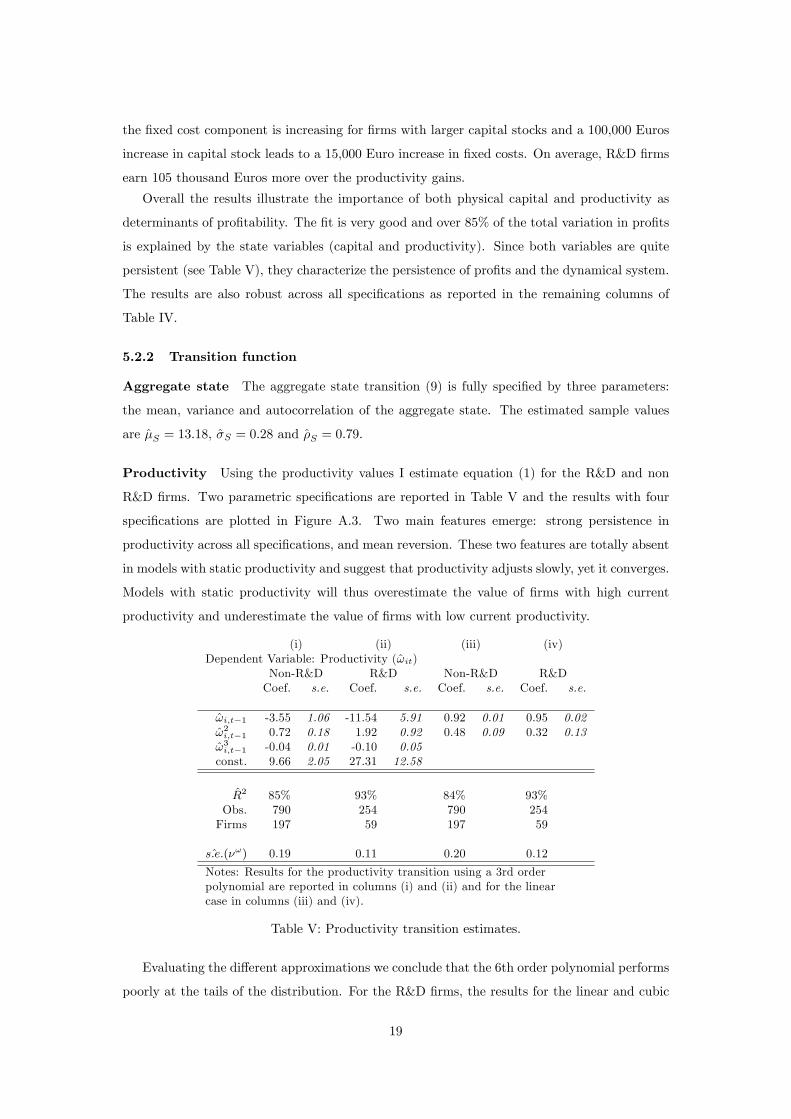
Productivity Using the productivity values I estimate equation (1) for the R&D and non

R&D �rms. Two parametric speci�cations are reported in Table V and the results with four

speci�cations are plotted in Figure A.3. Two main features emerge: strong persistence in

productivity across all speci�cations, and mean reversion. These two features are totally absent

in models with static productivity and suggest that productivity adjusts slowly, yet it converges.

Models with static productivity will thus overestimate the value of �rms with high current

productivity and underestimate the value of �rms with low current productivity.

(i) (ii) (iii) (iv)Dependent Variable: Productivity (!it)

Non-R&D R&D Non-R&D R&DCoef. s.e. Coef. s.e. Coef. s.e. Coef. s.e.

!i;t�1 -3.55 1.06 -11.54 5.91 0.92 0.01 0.95 0.02!2i;t�1 0.72 0.18 1.92 0.92 0.48 0.09 0.32 0.13!3i;t�1 -0.04 0.01 -0.10 0.05const. 9.66 2.05 27.31 12.58

R2 85% 93% 84% 93%Obs. 790 254 790 254Firms 197 59 197 59

^s:e:(�!) 0.19 0.11 0.20 0.12

Notes: Results for the productivity transition using a 3rd orderpolynomial are reported in columns (i) and (ii) and for the linearcase in columns (iii) and (iv).

Table V: Productivity transition estimates.

Evaluating the di¤erent approximations we conclude that the 6th order polynomial performs

poorly at the tails of the distribution. For the R&D �rms, the results for the linear and cubic

19

polynomials are similar, while the sigmoid function is non-stationary in the region with low

productivity. For the non-R&D �rms, the 6th order polynomial is again non-stationary as well

as the sigmoid function. The linear case does not give a good �t in the low productivity region

while the cubic polynomial �ts the data well both in terms of average �t (R2 = 85%) and at

the tails of the distribution.

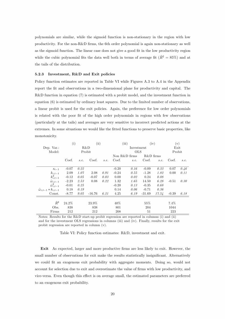
5.2.3 Investment, R&D and Exit policies

Policy function estimates are reported in Table VI while Figures A.3 to A.4 in the Appendix

report the �t and observations in a two-dimensional plane for productivity and capital. The

R&D function in equation (7) is estimated with a probit model, and the investment function in

equation (6) is estimated by ordinary least squares. Due to the limited number of observations,

a linear probit is used for the exit policies. Again, the preference for low order polynomials

is related with the poor �t of the high order polynomials in regions with few observations

(particularly at the tails) and averages are very sensitive to incorrect predicted actions at the

extremes. In some situations we would like the �tted functions to preserve basic properties, like

monotonicity.

(i) (ii) (iii) (iv) (v)Dep. Var.: R&D Investment Exit

Model: Probit OLS ProbitNon R&D �rms R&D �rms

Coef. s.e. Coef. s.e. Coef. s.e. Coef. s.e. Coef. s.e.

st�1 -0.07 0.22 -0.20 0.16 -0.09 0.33 0.07 0.46ki;t�1 2.09 1.07 2.08 0.91 -0.24 0.55 -1.28 1.82 0.00 0.11k2i;t�1 -0.12 0.05 -0.07 0.03 0.00 0.02 0.24 0.08!i;t�1 -2.23 2.53 0.08 0.22 1.32 1.65 14.50 6.28 -0.51 0.30!2i;t�1 -0.01 0.25 -0.20 0.13 -0.35 0.68

!i;t�1 � ki;t�1 0.18 0.19 0.14 0.06 -0.71 0.36Const. -8.77 9.05 -16.76 6.21 4.25 6.19 -31.69 17.54 -0.39 6.18

R2 24.2% 23.9% 40% 55% 7.4%Obs. 838 838 801 204 1044Firms 212 212 208 51 223

Notes: Results for the R&D start-up probit regression are reported in columns (i) and (ii)and for the investment OLS regressions in columns (iii) and (iv). Finally, results for the exitprobit regression are reported in column (v).

Table VI: Policy function estimates: R&D, investment and exit.

Exit As expected, larger and more productive �rms are less likely to exit. However, the

small number of observations for exit make the results statistically insigni�cant. Alternatively

we could �t an exogenous exit probability with aggregate moments. Doing so, would not

account for selection due to exit and overestimate the value of �rms with low productivity, and

vice-versa. Even though this e¤ect is on average small, the estimated parameters are preferred

to an exogenous exit probability.

20

R&D probit There are strong and signi�cant size e¤ects. Small �rms have a probability

of doing R&D close to zero, which increases strongly with capital and levels out for large capital

stocks (Figure A.2). The strong size e¤ect supports evidence for the potential gains from trade.

However, conditional on size there is no evidence that more productive �rms are more likely

to do R&D. The non signi�cant productivity e¤ect suggests the selection of more productive

�rms into R&D is not meaningful.

Investment For non-R&D �rms, investment is increasing in both size and productivity.

For R&D �rms, the size e¤ect is milder while the productivity e¤ect is stronger. This suggests

size-driven investment for non-R&D �rms, up until the optimal level. Once the optimal level

is reached and R&D is started, the size e¤ect becomes less pronounced and productivity is the

main driver of investment.

Summarizing, investment of non-R&D �rms is strongly in�uenced by size and productivity.

The R&D decision is a¤ected by size but not by productivity. Finally, large and more productive

�rms are less likely to exit, although none of the coe¢ cients in the exit probit is signi�cant.

Implications The results suggest the following model. Relatively more productive �rms

start by investing in physical capital. Once they reach a certain size, R&D becomes a prof-

itable investment. After R&D is done, productivity increases and since �rms are now larger,

investment rates decrease. The same mechanism is suggested by the descriptive statistics (Table

A.I). Growth rates are larger for non-R&D �rms (for sales, value added and labor productivity)

and investment rates are lower for R&D �rms. Furthermore, R&D �rms are larger and more

productive. Even though labor productivity growth is higher for non-R&D �rms, labor produc-

tivity level is higher for the R&D �rms. Taken together, these features characterize �rm level

dynamics and motivate the use of a dynamic model with productivity and capital investment.

5.3 Third step

The minimum distance estimator outlined above is now implemented to recover the dynamic

parameters reported in the �rst row (model 1) of Table VII: the linear and quadratic invest-

ment cost, R&D sunk cost and exit value. Con�dence intervals were constructed using the

bootstrap.16

The values are estimated with the expected signs. Sunk costs are estimated at about 3.4

million Euros, almost two times the average sales and more than one year worth of sales for an

16Step 3 only produces simulation error. This error is reduced as the number of simulation draws increase(nJ ! 1). Since bootstrapping requires intense computations, the number of simulations is kept within amanageable value and set nJ = 125. The bootstrapped con�dence intervals will thus contain some noise fromthe simulations.

21

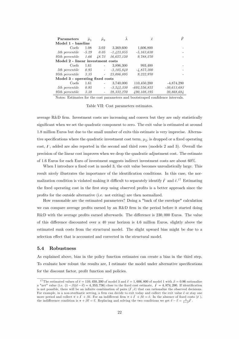
Parameters �1 �2 � e FModel 1 - baseline

Coefs 1.08 3.02 3,369,600 1,606,800 -5th percentile -5.29 0.05 -1,423,855 -5,163,630 -95th percentile 1.66 48.73 16,657,150 9,788,270 -Model 2 - linear investment costs

Coefs 1.61 - 3,896,300 993,400 -5th percentile 0.95 - -3,105,840 -4,857,300 -95th percentile 3.35 - 23,086,895 9,222,970 -Model 3 - operating �xed costs

Coefs 1.61 - 3,740,000 110,450,200 -4,874,2905th percentile 0.95 - -3,542,330 -692,556,855 -30,613,68395th percentile 3.38 - 28,332,270 490,108,195 20,868,684

Notes: Estimates for the cost parameters and bootstraped con�dence intervals.

Table VII: Cost parameters estimates.

average R&D �rm. Investment costs are increasing and convex but they are only statistically

signi�cant when we set the quadratic component to zero. The exit value is estimated at around

1.8 million Euros but due to the small number of exits this estimate is very imprecise. Alterna-

tive speci�cations where the quadratic investment cost term, �2, is dropped or a �xed operating

cost, z, added are also reported in the second and third rows (models 2 and 3). Overall the

precision of the linear cost improves when we drop the quadratic adjustment cost. The estimate

of 1.6 Euros for each Euro of investment suggests indirect investment costs are about 60%.When I introduce a �xed cost in model 3, the exit value becomes unrealistically large. This

result nicely illustrates the importance of the identi�cation conditions. In this case, the nor-

malization condition is violated making it di¢ cult to separately identify z and e.17 Estimating

the �xed operating cost in the �rst step using observed pro�ts is a better approach since the

pro�ts for the outside alternative (i.e. not exiting) are then normalized.How reasonable are the estimated parameters? Doing a "back of the envelope" calculation

we can compare average pro�ts earned by an R&D �rm in the period before it started doing

R&D with the average pro�ts earned afterwards. The di¤erence is 230; 000 Euros. The value

of this di¤erence discounted over a 40 year horizon is 4.6 million Euros, slightly above the

estimated sunk costs from the structural model. The slight upward bias might be due to a

selection e¤ect that is accounted and corrected in the structural model.

5.4 Robustness

As explained above, bias in the policy function estimates can create a bias in the third step.

To evaluate how robust the results are, I estimate the model under alternative speci�cations

for the discount factor, pro�t function and policies.

17The estimated values of e = 110; 450; 200 of model 3 and ee = 1; 606; 800 of model 1 with � = 0:96 rationalizea "net" value (i.e. (1� �)(e� ee) = 4; 353; 736) close to the �xed cost estimate, z = 4; 874; 290. If identi�cationis not possible, there will be an in�nite combination of pairs (z; e) that can rationalize the observed decisions.For example, in a non-stochastic setting, a �rm can decide to exit today and collect the exit value e or stay onemore period and collect � + z+ �e. For an indi¤erent �rm � + z+ �e = e. In the absence of �xed costs (z),the indi¤erence condition is � + �ee = ee. Replacing and solving the two conditions we get e� ee = 1

1�� z.

22

Discount factor Lower discount factors reduce the continuation value and, as expected,

decrease the estimated investment and sunk costs. For example, with a discount factor of 0.9

the sunk costs are estimated at 1.2 million Euros and the investment costs at 0:83 for the linear

and 1:41 for the quadratic component.

� �1 �2 � e

0.90 0.83 1.41 1,299,200 -574,5000.91 0.87 1.58 1,477,800 -504,1000.92 0.91 1.77 1,702,700 -368,3000.93 0.95 2.00 1,989,500 -131,9000.94 1.00 2.27 2,355,300 264,1000.95 1.04 2.61 2,808,200 835,7000.96 1.08 3.02 3,368,800 1,607,7000.97 1.12 3.51 4,028,200 2,731,0000.98 1.15 4.16 4,355,900 4,733,3000.99 1.13 5.10 3,042,900 8,481,800

Table VIII: Cost parameters estimates for di¤erent discount factors.

Pro�t function Estimated dynamic cost parameters are also quite robust when the al-

ternative reduced form pro�t functions from Table IV are used. Overall, the sunk costs are

estimated between 1.1 and 3.7 million Euros while the investment costs are only marginally

a¤ected.

�1 �2 � eBaseline 1.08 3.02 3,369,600 1,606,800�6 = 0 1.03 3.27 1,111,600 1,156,500

�5 = �6 = 0 1.16 2.77 1,423,500 1,922,300�4 = �5 = �6 = 0 1.16 2.77 1,403,600 1,946,700

�5 = 0 1.17 2.70 3,672,700 1,979,000

Table IX: Cost parameters estimates for di¤erent speci�cations of the pro�t function.

Policy functions The policy functions play a central role in the estimation. Due to the

nonlinearities, even small bias in the estimated policies can get magni�ed into a large bias in the

structural parameters. To evaluate how sensitive the results are, I try simpler (linear) policies.

Using a linear investment function, sunk cost are estimated at about 3 million Euros and

investment costs at �1:98 for the linear and 29:09 for the quadratic component. Alternatively,

using a linear probit for R&D, sunk cost are estimated at 4.5 million Euros and adjustment costs

at 1:18 for the linear and 2:01 for the quadratic component. If we allow both the investment

and R&D policies to be linear, the sunk cost is estimated at 2.9 millions.

Overall, the results are relatively robust to alternative speci�cations. A �nal validation

exercise is to evaluate how well the estimated model matches the actual data.

23

�1 �2 � e

Linear R&D probit 1.18 2.01 4,475,100 -992,000Linear investment -1.98 29.09 2,987,600 1,174,100

Linear R&D probit and investment -1.64 26.98 2,920,100 1,489,900

Table X: Cost parameters estimates for di¤erent policy functions.

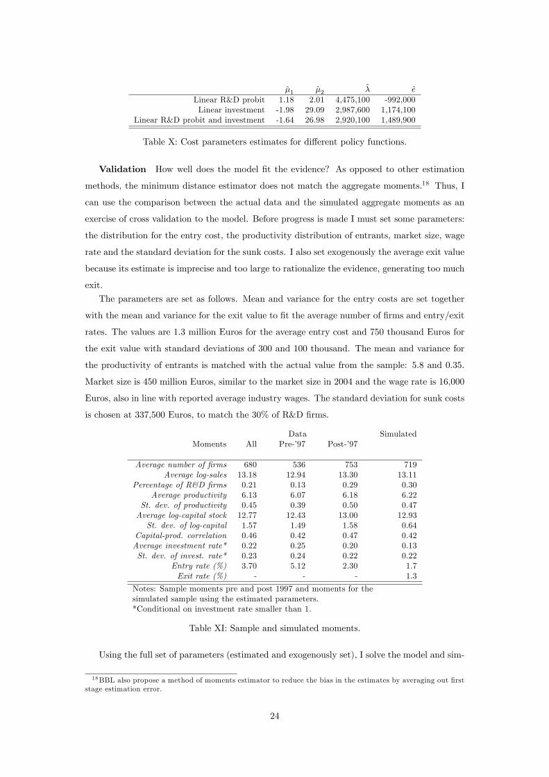
Validation How well does the model �t the evidence? As opposed to other estimation

methods, the minimum distance estimator does not match the aggregate moments.18 Thus, I

can use the comparison between the actual data and the simulated aggregate moments as an

exercise of cross validation to the model. Before progress is made I must set some parameters:

the distribution for the entry cost, the productivity distribution of entrants, market size, wage

rate and the standard deviation for the sunk costs. I also set exogenously the average exit value

because its estimate is imprecise and too large to rationalize the evidence, generating too much

exit.

The parameters are set as follows. Mean and variance for the entry costs are set together

with the mean and variance for the exit value to �t the average number of �rms and entry/exit

rates. The values are 1.3 million Euros for the average entry cost and 750 thousand Euros for

the exit value with standard deviations of 300 and 100 thousand. The mean and variance for

the productivity of entrants is matched with the actual value from the sample: 5.8 and 0.35.

Market size is 450 million Euros, similar to the market size in 2004 and the wage rate is 16,000

Euros, also in line with reported average industry wages. The standard deviation for sunk costs

is chosen at 337,500 Euros, to match the 30% of R&D �rms.

Data SimulatedMoments All Pre-�97 Post-�97

Average number of �rms 680 536 753 719Average log-sales 13.18 12.94 13.30 13.11

Percentage of R&D �rms 0.21 0.13 0.29 0.30Average productivity 6.13 6.07 6.18 6.22

St. dev. of productivity 0.45 0.39 0.50 0.47Average log-capital stock 12.77 12.43 13.00 12.93St. dev. of log-capital 1.57 1.49 1.58 0.64

Capital-prod. correlation 0.46 0.42 0.47 0.42Average investment rate* 0.22 0.25 0.20 0.13St. dev. of invest. rate* 0.23 0.24 0.22 0.22

Entry rate (%) 3.70 5.12 2.30 1.7Exit rate (%) - - - 1.3

Notes: Sample moments pre and post 1997 and moments for thesimulated sample using the estimated parameters.*Conditional on investment rate smaller than 1.

Table XI: Sample and simulated moments.

Using the full set of parameters (estimated and exogenously set), I solve the model and sim-

18BBL also propose a method of moments estimator to reduce the bias in the estimates by averaging out �rststage estimation error.

24

ulate the industry for 120 periods. To do the simulations I am now required to solve the model

and calculate the new equilibrium industry evolution, q(St; St+1). The computational burden

of solving a full dynamic game would be prohibitive while I can solve the proposed aggregate

state model in a reasonable time.19 After dropping the �rst 60 periods I calculate the moments

for the stationary market structure, reported in Table XI: the mean and standard deviation

for productivity, capital, and investment rate, and the correlation between productivity and

capital. Also reported are the number of �rms, aggregate state and entry rate but these values

are not free since, as explained, they where "calibrated" by setting the distributions of entry

and exit values.

The model can explain well the �rst and second moments for capital and productivity but

generates too little variation in capital. The little variation in capital is probably because all

�rms are ex-ante identical and there is no source of persistent unobserved heterogeneity in the

model. The model does not provide such a good �t for the investment rates. This is because

we observe a high investment transition period. If we consider only the later years (after 2000),

investment rates and variation decrease to 0.13 and 0.18, more in line with the predicted values.

Finally, the model explains well the correlation between capital and productivity. Using these

values as a benchmark, we can now evaluate the e¤ects of some policy changes.

6 Counterfactual Experiments

This section reports the results for three policy experiments to assess the impact on industry

R&D, productivity and investment. The experiments consist of changes in (i) market size, (ii)

sunk costs of R&D, and (iii) entry costs. Because the model is stylized, the particular numbers

generated by the counterfactual simulations should be seen as merely suggestive as the e¤ects

of any policy change might depend on other factors not captured by the model.20

Reduction in market size The goal is to access the models�predictions in case we return

to the pre-trade liberalization era, by evaluating the e¤ects of a reduction in market size. I

can use changes in market size as a parallel for changes in trade barriers because the internal

market is small and the industry has always been a heavy exporter. In particular, since 90%

of total production is exported, I can abstract from import competition e¤ects. One implicit

assumption is that foreign competitors do not react to changes at the national level. Since

Portugal is a small country, worldwide industry structure is unlikely to be a¤ected by changes

19A MATLAB algorithm to solve the model is available from the author. Solving the model takes about 120minutes on a 2.6 Ghz Phenom Quad-core computer with 3GB RAM.20Also, the standard deviation of the payo¤ shocks is not identi�ed and this object in�uences the magnitude

(but not the sign) of the e¤ects. This is particularly relevant for the sunk costs of R&D where we identify theaverage cost paid by a �rm who decided to do R&D and not the average unconditional cost. A decrease in theconditional mean is stronger than an equivalent decrease in the unconditional mean.

25

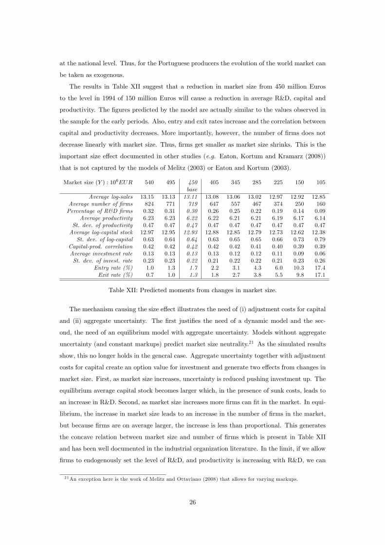
at the national level. Thus, for the Portuguese producers the evolution of the world market can

be taken as exogenous.

The results in Table XII suggest that a reduction in market size from 450 million Euros

to the level in 1994 of 150 million Euros will cause a reduction in average R&D, capital and

productivity. The �gures predicted by the model are actually similar to the values observed in

the sample for the early periods. Also, entry and exit rates increase and the correlation between

capital and productivity decreases. More importantly, however, the number of �rms does not

decrease linearly with market size. Thus, �rms get smaller as market size shrinks. This is the

important size e¤ect documented in other studies (e.g. Eaton, Kortum and Kramarz (2008))

that is not captured by the models of Melitz (2003) or Eaton and Kortum (2003).

Market size (Y ) : 106EUR 540 495 450 405 345 285 225 150 105base

Average log-sales 13.15 13.13 13.11 13.08 13.06 13.02 12.97 12.92 12.85Average number of �rms 824 771 719 647 557 467 374 250 160Percentage of R&D �rms 0.32 0.31 0.30 0.26 0.25 0.22 0.19 0.14 0.09

Average productivity 6.23 6.23 6.22 6.22 6.21 6.21 6.19 6.17 6.14St. dev. of productivity 0.47 0.47 0.47 0.47 0.47 0.47 0.47 0.47 0.47Average log-capital stock 12.97 12.95 12.93 12.88 12.85 12.79 12.73 12.62 12.38St. dev. of log-capital 0.63 0.64 0.64 0.63 0.65 0.65 0.66 0.73 0.79

Capital-prod. correlation 0.42 0.42 0.42 0.42 0.42 0.41 0.40 0.39 0.39Average investment rate 0.13 0.13 0.13 0.13 0.12 0.12 0.11 0.09 0.06St. dev. of invest. rate 0.23 0.23 0.22 0.21 0.22 0.22 0.21 0.23 0.26

Entry rate (%) 1.0 1.3 1.7 2.2 3.1 4.3 6.0 10.3 17.4Exit rate (%) 0.7 1.0 1.3 1.8 2.7 3.8 5.5 9.8 17.1

Table XII: Predicted moments from changes in market size.

The mechanism causing the size e¤ect illustrates the need of (i) adjustment costs for capital

and (ii) aggregate uncertainty. The �rst justi�es the need of a dynamic model and the sec-

ond, the need of an equilibrium model with aggregate uncertainty. Models without aggregate

uncertainty (and constant markups) predict market size neutrality.21 As the simulated results

show, this no longer holds in the general case. Aggregate uncertainty together with adjustment

costs for capital create an option value for investment and generate two e¤ects from changes in

market size. First, as market size increases, uncertainty is reduced pushing investment up. The

equilibrium average capital stock becomes larger which, in the presence of sunk costs, leads to

an increase in R&D. Second, as market size increases more �rms can �t in the market. In equi-

librium, the increase in market size leads to an increase in the number of �rms in the market,

but because �rms are on average larger, the increase is less than proportional. This generates

the concave relation between market size and number of �rms which is present in Table XII

and has been well documented in the industrial organization literature. In the limit, if we allow

�rms to endogenously set the level of R&D, and productivity is increasing with R&D, we can

21An exception here is the work of Melitz and Ottaviano (2008) that allows for varying markups.

26

have a Sutton (1998) style e¤ect where industry concentration is bounded below as market size

increases.

Reduction in the sunk costs of R&D A reduction in sunk costs can also have e¤ects

on productivity and trade. An example of a policy to reduce the sunk costs is a direct subsidy

to R&D start-up. Other, more general, policies could be more e¤ective in reducing sunk costs.

For example, a public R&D lab could explore economies of scale and avoid R&D duplication

costs. The results in Table XIII show that a reduction in sunk costs is expected to lead to

an increase in R&D, productivity, capital and investment. More importantly average sales are

increasing which suggests that reducing the sunk costs of R&D can also promote �rm exports.

These e¤ects are similar to an increase in market size and either of them is able to rationalize

the observed industry change.

Sunk costs (�) : 106EUR 2.89 3.06 3.23 3.32 3.40 3.57 3.74 4.08 4.42base

Average log-sales 13.23 13.19 13.13 13.14 13.10 13.06 13.07 13.06 13.05Average number of �rms 1000 991 893 792 714 621 576 563 552Percentage of R&D �rms 0.98 0.88 0.60 0.46 0.29 0.11 0.03 0.01 0.00

Average productivity 6.36 6.34 6.28 6.25 6.22 6.19 6.17 6.17 6.16St. dev. of productivity 0.42 0.43 0.45 0.46 0.46 0.47 0.47 0.47 0.47Average log-capital stock 13.44 13.36 13.14 13.06 12.92 12.80 12.76 12.74 12.73St. dev. of log-capital 0.66 0.65 0.68 0.68 0.63 0.56 0.54 0.52 0.51

Capital-prod. correlation 0.39 0.40 0.44 0.44 0.41 0.37 0.35 0.34 0.33Average investment rate 0.14 0.14 0.14 0.13 0.13 0.12 0.12 0.12 0.11St. dev. of invest. rate 0.31 0.29 0.26 0.24 0.22 0.19 0.19 0.18 0.17

Entry rate (%) 0.0 0.1 0.6 1.2 1.7 2.5 2.9 3.0 3.2Exit rate (%) 0.0 0.0 0.4 0.9 1.3 2.0 2.5 2.6 2.7

Table XIII: Predicted moments from changes in sunk costs of R&D.

Reducing the sunk costs only a¤ects the value of non-R&D �rms and leaves the value of

R&D �rms unchanged (excluding equilibrium e¤ects). Changes in sunk costs a¤ect the value

function through three di¤erent mechanisms. First, smaller sunk costs cause a direct reduction

in costs. Second, the probability of doing R&D increases with a decrease in sunk costs having an

indirect e¤ect and increasing expected bene�ts. Finally, there are the equilibrium e¤ects that

operates in the opposite way in the value function. As sunk costs decrease, the value of entering

is increased and more �rms enter the market leading to an increase in the number of �rms. The

decrease in sunk costs leads to an increase in R&D and productivity. As a consequence, �rms

invest more and become larger. Summarizing, a decrease in the sunk costs lead to more �rms

in equilibrium that are on average larger and more productive.

Increase in entry costs Lastly, there is often political support for the creation of large

�rms under the argument that this might spur innovation. One way to create large �rms is by

increasing entry costs. Large entry costs will decrease entry rates and protect incumbent �rms

27

from competition, allowing them to grow. Larger �rms will then be willing to pay the sunk

cost and start innovating.

As reported in Table XIV, an increase in entry costs boosts innovation by generating an

increase in average size, investment and R&D. However, it also leads to a reduction in the

number of �rms and entry/exit rates and bad �rms are now less likely to exit and be replaced

by better �rms. Overall, this selection e¤ect might lead to a decrease in average industry

productivity, specially if the boost in innovation is not su¢ ciently strong (or all �rms are already

innovating). As expected, the increase in entry costs protects �rms and leads to an increase

in average size. Alternatively, increasing entry costs during a trade liberalization period could

mitigate the negative competition e¤ects from the increase in entry costs, while still keeping

the positive e¤ects from trade liberalization.

Entry costs (e) : 106EUR 0.98 1.04 1.17 1.3 1.43 1.56 1.63 1.69base

Average log-sales 12.94 12.98 13.02 13.10 13.19 13.26 13.32 13.36Average number of �rms 876 815 778 713 661 646 629 599Percentage of R&D �rms 0.16 0.21 0.25 0.29 0.37 0.46 0.51 0.57

Average productivity 6.19 6.21 6.22 6.22 6.24 6.25 6.26 6.27St. dev. of productivity 0.47 0.47 0.47 0.46 0.46 0.46 0.45 0.44Average log-capital stock 12.71 12.82 12.87 12.92 13.00 13.10 13.18 13.23St. dev. of log-capital 0.68 0.64 0.62 0.64 0.65 0.67 0.70 0.70

Capital-prod. correlation 0.39 0.40 0.41 0.41 0.42 0.44 0.44 0.41Average investment rate 0.10 0.12 0.12 0.13 0.13 0.14 0.14 0.14St. dev. of invest. rate 0.22 0.22 0.21 0.22 0.23 0.26 0.28 0.27

Entry rate (%) 6.7 4.0 2.6 1.7 1.0 0.5 0.3 0.3Exit rate (%) 6.5 3.8 2.3 1.3 0.5 0.1 0.1 0.0

Table XIV: Predicted moments from changes in entry costs.

7 Conclusion

The evidence suggests that technology is endogenous and size is an important explanation for

the technology decision. I have proposed and estimated an equilibrium model with endogenous

choices of technology and size. One disadvantage compared with simpler models is the lack of

analytical solutions. I estimate the model for a sample of �rms from the Portuguese moulds

industry and �nd evidence of relatively large sunk costs of R&D. These costs are particularly

relevant in this industry since �rms are very small. Getting access to large markets allows

the �rms to exploit the economies of scale in R&D and introduce more innovations. Overall,

sunk costs explain why R&D is done by larger �rms and why successful �rms invest in physical

capital before doing R&D. The two results put together can explain the observed performance

of some industries after trade liberalization episodes, like the Portuguese moulds industry.

There are some challenging questions left unanswered. First, how relevant are the sunk costs

on a macro scale. The existence of sunk costs can be relevant on a macroeconomic level if they are

28

important within each industry. Second, the model proposed here is partial equilibrium. A trade

liberalization event will certainly trigger other general equilibrium e¤ects on wages and returns

on capital. How these e¤ects a¤ect the innovation decisions is a question to be considered.

Third and �nally, the model does not incorporate persistent unobserved heterogeneity either

in returns or costs. Incorporating persistent heterogeneity in dynamic models is probably the

most important question to be addressed in the future.

A Appendix

A.1 Sample construction and descriptive statistics

The sample comes from three sources: Aggregate variables (sales, value added, employment)

come from the Portuguese National Statistics O¢ ce (INE); industry price de�ators are collected

from IAPMEI (2006); and the �rm level sample was extracted from the Bank of Portugal

database on �rms across the economy (Central de Balancos, �ve digit NACE code industry

29563 - moulds industry).

Some notes on the Central de Balancos: The sample has been collected by the Central

Bank since 1986. However, due to changes in accounting rules, it is only comparable from 1990.

The data between 1990 and 1994 is not considered reliable. From 2000 the sampling method

(simple random sampling) was changed to strati�ed sampling causing a drop in the number of

observed (mostly smaller) �rms in 1999 and 2000.

Representativeness: The sample is representative of the whole industry, in particular

for the early periods. It covers 90% of total sales and industry employment in 1994 and the

coverage decreases to a minimum of 50% of sales (40% of employment) in 2003. This reduction

is mainly due to changes in the sampling procedure as explained above. There is an obvious gap

in productivity trends between the sample and the industry (also total sales and employment).

Labor productivity increased by roughly 60% in the sample and only 40% in the industry. None

of the aggregate variables are calculated using the sample but come directly from the collected

industry wide variables.

Variable construction:

Capital stock was calculated using the perpetual inventory method with a 8% depreciation

rate

Ki;t+1 = (1� depreciation) �Kit + Ii;t+1

Value added is equal to sales subtracted from materials and external services expenditures

V Ait = Yit �Mit � ESEit

29

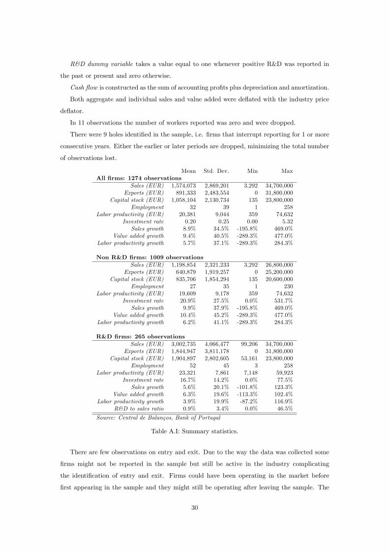
R&D dummy variable takes a value equal to one whenever positive R&D was reported in

the past or present and zero otherwise.

Cash �ow is constructed as the sum of accounting pro�ts plus depreciation and amortization.

Both aggregate and individual sales and value added were de�ated with the industry price

de�ator.

In 11 observations the number of workers reported was zero and were dropped.

There were 9 holes identi�ed in the sample, i.e. �rms that interrupt reporting for 1 or more

consecutive years. Either the earlier or later periods are dropped, minimizing the total number

of observations lost.

Mean Std. Dev. Min MaxAll �rms: 1274 observations

Sales (EUR) 1,574,073 2,869,201 3,292 34,700,000Exports (EUR) 891,333 2,483,554 0 31,800,000

Capital stock (EUR) 1,058,104 2,130,734 135 23,800,000Employment 32 39 1 258

Labor productivity (EUR) 20,381 9,044 359 74,632Investment rate 0.20 0.25 0.00 5.32Sales growth 8.9% 34.5% -195.8% 469.0%

Value added growth 9.4% 40.5% -289.3% 477.0%Labor productivity growth 5.7% 37.1% -289.3% 284.3%

Non R&D �rms: 1009 observationsSales (EUR) 1,198,854 2,321,233 3,292 26,800,000

Exports (EUR) 640,879 1,919,257 0 25,200,000Capital stock (EUR) 835,706 1,854,294 135 20,600,000

Employment 27 35 1 230Labor productivity (EUR) 19,609 9,178 359 74,632

Investment rate 20.9% 27.5% 0.0% 531.7%Sales growth 9.9% 37.9% -195.8% 469.0%

Value added growth 10.4% 45.2% -289.3% 477.0%Labor productivity growth 6.2% 41.1% -289.3% 284.3%

R&D �rms: 265 observationsSales (EUR) 3,002,735 4,066,477 99,206 34,700,000

Exports (EUR) 1,844,947 3,811,178 0 31,800,000Capital stock (EUR) 1,904,897 2,802,605 53,161 23,800,000

Employment 52 45 3 258Labor productivity (EUR) 23,321 7,861 7,148 59,923

Investment rate 16.7% 14.2% 0.0% 77.5%Sales growth 5.6% 20.1% -101.8% 123.3%

Value added growth 6.3% 19.6% -113.3% 102.4%Labor productivity growth 3.9% 19.9% -87.2% 116.9%

R&D to sales ratio 0.9% 3.4% 0.0% 46.5%

Source: Central de Balanços, Bank of Portugal

Table A.I: Summary statistics.

There are few observations on entry and exit. Due to the way the data was collected some

�rms might not be reported in the sample but still be active in the industry complicating

the identi�cation of entry and exit. Firms could have been operating in the market before

�rst appearing in the sample and they might still be operating after leaving the sample. The

30

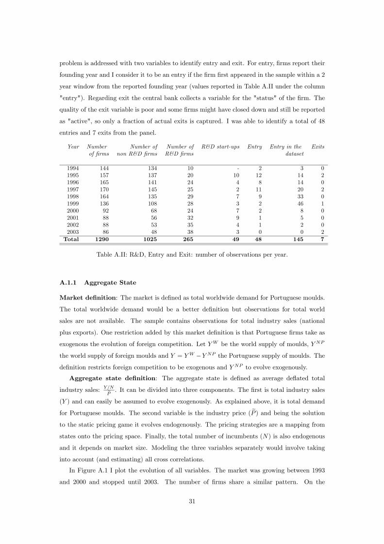
problem is addressed with two variables to identify entry and exit. For entry, �rms report their

founding year and I consider it to be an entry if the �rm �rst appeared in the sample within a 2

year window from the reported founding year (values reported in Table A.II under the column

"entry"). Regarding exit the central bank collects a variable for the "status" of the �rm. The

quality of the exit variable is poor and some �rms might have closed down and still be reported

as "active", so only a fraction of actual exits is captured. I was able to identify a total of 48

entries and 7 exits from the panel.

Year Number Number of Number of R&D start-ups Entry Entry in the Exitsof �rms non R&D �rms R&D �rms dataset

1994 144 134 10 - 2 3 01995 157 137 20 10 12 14 21996 165 141 24 4 8 14 01997 170 145 25 2 11 20 21998 164 135 29 7 9 33 01999 136 108 28 3 2 46 12000 92 68 24 7 2 8 02001 88 56 32 9 1 5 02002 88 53 35 4 1 2 02003 86 48 38 3 0 0 2Total 1290 1025 265 49 48 145 7

Table A.II: R&D, Entry and Exit: number of observations per year.

A.1.1 Aggregate State

Market de�nition: The market is de�ned as total worldwide demand for Portuguese moulds.

The total worldwide demand would be a better de�nition but observations for total world

sales are not available. The sample contains observations for total industry sales (national

plus exports). One restriction added by this market de�nition is that Portuguese �rms take as

exogenous the evolution of foreign competition. Let YW be the world supply of moulds, Y NP

the world supply of foreign moulds and Y = YW �Y NP the Portuguese supply of moulds. The

de�nition restricts foreign competition to be exogenous and Y NP to evolve exogenously.

Aggregate state de�nition: The aggregate state is de�ned as average de�ated total

industry sales: Y=NeP . It can be divided into three components. The �rst is total industry sales

(Y ) and can easily be assumed to evolve exogenously. As explained above, it is total demand

for Portuguese moulds. The second variable is the industry price ( eP ) and being the solutionto the static pricing game it evolves endogenously. The pricing strategies are a mapping from

states onto the pricing space. Finally, the total number of incumbents (N) is also endogenous

and it depends on market size. Modeling the three variables separately would involve taking

into account (and estimating) all cross correlations.

In Figure A.1 I plot the evolution of all variables. The market was growing between 1993

and 2000 and stopped until 2003. The number of �rms share a similar pattern. On the

31

other side prices were increasing slightly and decreased in the later years. The industry grew

substantially after 1994 due to the strong increase in demand for Portuguese moulds. We also

observe an increase in labor productivity and R&D. The cross correlations are as expected

with prices being negatively correlated with number of �rms and market size, and the number

of �rms being positively correlated with market size. The evolution of the three variables is

summarized by the evolution of the single index variable, eYeP (average de�ated sales).

Number Production Exports Exports Employment Value Added Priceof �rms (EUR mio) (EUR mio) % of sales (EUR mio) (EUR/ton)

1994 644 171 132 77% 5,133 101 24.431995 570 193 151 78% 5,796 114 25.251996 452 244 191 78% 7,316 143 25.711997 477 293 220 75% 7,821 166 25.731998 461 322 232 72% 7,740 167 24.621999 549 362 250 69% 8,429 208 25.232000 604 412 277 67% 8,879 228 26.492001 612 421 328 78% 8,919 240 26.742002 722 378 310 82% 9,312 235 24.972003 738 403 303 75% 8,766 227 22.862004 1109 455 340 . 9,846 259 20.332005 1230 468 298 . 10,108 256 18.69

Source: National statistics o¢ ce, INE (2007)

Table A.III: Aggregate variables

0

200

400

600

800

1000

1200

1994 1995 1996 1997 1998 1999 2000 2001 2002 2003 2004 2005

Number of f irms Total Sales (EUR mios)Price index (1995=1000) Average deflated sales (EUR th)

Figure A.1: Aggregate variables: Number of �rms, price index, average and total sales

32

A.2 Production function estimation

Here, I explain how total factor productivity is estimated. Productivity is not directly observed

and there are several available methods to estimate it as the residual from a production function.

De Loecker (2007) proposes an estimator for both the production function parameters and the

demand elasticity under imperfect competition when one uses de�ated sales instead of quantities

(see also Klette and Griliches (1995). The estimator, however, cannot be directly applied to

an equilibrium model.22 Input demand functions depend on the industry state, more precisely,

the aggregate industry state. For example investment functions depend on equilibrium beliefs

about industry evolution. Specifying the investment policy as originally proposed by Olley and

Pakes (1996), i(!), is a misspeci�cation since the equilibrium policy for investment in a Markov

Perfect Equilibrium depends on the state of all players in the industry i�(!1; ::; !N ). Therefore,

elasticity of demand cannot be recovered in the �rst step as proposed by De Loecker (2007) since

the input demand is also a function of aggregate sales.23 Using a Cobb-Douglas production

function with labor and capital (Q = e!iL�lK�k), adding a demand function (Q = ~Y~P

�P~P

���)

with market size ( ~Y ) and price index ( ~P ) and taking the logs of �rm level de�ated sales (PitQit

~P)

yit � ~pt = qit + pit � ~pt =1

�(~yt � ~pt) +

� � 1�

(!it + �kkit + �llit) (A.1)

Using materials to control for the unobservable as in Levinsohn and Petrin (2003), the input

demand is a function of the state at time t (individual and industry states)

mit = m(!it; kit; Rit; St) (A.2)

Assuming invertibility24

!it = !(kit; Rit; St;mit) (A.3)

Since productivity is also a function of market conditions (St =~Yt~Pt) in equation (A.2),

demand elasticity (�) is not identi�ed in the �rst stage, because it enters nonlinearly in the

control function (A.3). This is the main di¤erence from a single agent framework as in

22This is the true for most methods with similar approaches to Olley and Pakes (1996). Such methods look atsingle agent problems and disregard the possibility that policy functions (investment or materials) are equilibriumsolutions to dynamic games. Therefore, the policy functions will be misspeci�ed and the productivity controlfunction will not include some important industry level variables leading to bias in the parameter estimates dueto unobserved heterogeneity. How large this bias is in practice is an empirical question.23There is also the selection problem due to exit as explained in Olley and Pakes (1996). In this paper I will

abstract from this problem since the number of exits observed in the data is very small and the correction doesnot a¤ect my estimates. However, if there were more observations on exits, this problem could be more carefullyaddressed.24With imperfect competition an increase in productivity might not lead to an increase in output and there-

fore in materials usage causing concerns over invertibility. For the demand system speci�ed, an increase inproductivity is equivalent to a decrease in costs and it translates in a decrease in prices. Both total output andmaterials usage increase.

33

De Loecker (2007) where input demand depends solely on individual state variables (mit =

m(!it; kit; Rit)). Using the controlled �rst order Markov process assumption for productivity

!it = E[!itj!it�1; Rit�1] + �!it.

A.2.1 Stage I

From eq. (A.1) using de�ated sales as variables ypit = yit � ~pt and ~ypt = ~yt � ~pt = ln(St) the

production function is

ypit =� � 1�

�llit + �(kit; Rit; ~ypt ;mit) + y

"it (A.4)

where y"it is measurement error in ypit, and

\��1� �l and � can be estimated nonparametrically

or using an nth-order polynomial approximation from

�(kit; Rit; ~ypt ;mit) =

1

�~ypt +

� � 1�

�kkit +� � 1�

!(kit; Rit; ~ypt ;mit)

A.2.2 Stage II

Let the estimated value be �it = ypit �

\��1� �

llit. An estimate of

��1� !it for a given

��1� �k ande1

� is

\� � 1�

!it = �it �e1�~ypt �

^� � 1�

�kkit

Approximate E[!itj!it�1; Rit�1] with an nth-order polynomial Pn;!(!it�1; Rit�1). Several

approximations are used in the empirical section and in practice a cubic polynomial provides a

good �t, in particular at the tails of the observations25

ypit �\� � 1�

�llit =1

�~ypt +

� � 1�

�kkit + (A.5)

+Pn;!(!it�1; Rit�1) + �!it

Finally, 1� and �k are estimated by nonlinear least squares using eq. (A.5).

A.2.3 Results

Estimates are reported in Table A.IV.26 The estimated labor and capital coe¢ cients are 0.51 and

0.4, while the estimated demand elasticity implies a price-cost margin of 8%. The values are at a

25 Instead of using a cubic polynomial, also reported are the results with a sigmoidal function which preservesmonotonicity: E(!itj!i;t�1) = 0

(1+ 1 exp(�!i;t�1))26The results are reported for value added production functions. The approach is identical to the one using

sales under the assumption that materials are a constant share of total sales. Since by de�nition Yit = V Ait+Mit,if Mit = �mYit then Yit = V Ait + �mYit so that Yit = 1

(1��m)V Ait.

34

(i) (ii) (iii) (iv) (v) (vi)1st stage 2nd stage 2nd stage 2nd stage Fixed E¤ects

Equation: (A.4) (A.5) (A.5) (A.5) (A.1) (A.1)Model: OLS NLLS NLLS NLLS FE FE

Cubic Linear Sigmoidal ControlApprox. Approx. Approx. function

Coef. s.e. Coef. s.e. Coef. s.e. Coef. s.e. Coef. s.e. Coef. s.e.lit 0.47 0.04 0.69 0.04 0.52 0.04kit 0.37 0.02 0.41 0.03 0.38 0.02 0.37 0.03~ypt 0.08 0.04 0.07 0.05 0.07 0.04

const. 3.57 0.64

R2 98% 92% 92% 92% 92% 93%Obs. 1,271 1,044 1,044 1,044 1,271 1271Firms 227 223 223 223 227 227

Labor coef. 0.51 0.51 0.74 0.69Capital coef. 0.40 0.44 0.40 0.37 -Price Cost Margin 8% 7% 7% - -

Notes: Results for the �rst stage of the production function estimates are reported in column (i).Columns (ii)-(iv) report the second stage estimates using a cubic, linear and sigmoidalapproximation, respectively. Column (v) reports the results for the �xed e¤ects speci�cationwith year dummies. The speci�cation in column (vi) is identical to column (i) with added �xed e¤ects.

Table A.IV: Production function estimates.

reasonable level and within the range of parameters found in the literature for other industries.

In columns (iii) and (iv) results are also reported for a linear and a sigmoid parametrization

for productivity transition. The advantage is that both preserve monotonicity. Overall the

di¤erences are negligible and there is no evidence that functional forms are restrictive.

Results using alternative methods are also reported. In particular using a simple �xed e¤ects

speci�cation with time dummies (column (v)) does not perform well due to serial correlation

in productivity. Adding the control function E[!itj!it�1; Rit�1] in column (vi) reduces the

magnitude of the labor coe¢ cient suggesting the �xed e¤ects and time dummies are not properly

capturing the correlation between labor and productivity

A.3 Figures

68

1012

1416

4

5

6

7

8

0

0.05

0.1

0.15

0.2

0.25

Capital

R&D probit

Productivity

Figure A.2: R&D probit, �t in productivity and capital space

35

Figure A.3: Productivity transition (observations and �t)

Figure A.4: Investment functions, �t in productivity and capital space

36

References

[1] Ackerberg, D., L. Benkard, S. Berry, and A. Pakes (2007): �Econometric Tools for Ana-

lyzing Market Outcomes�, in Handbook of Econometrics, vol. 6, ch. 63, ed. by J. Heckman

and E. Leamer.

[2] Aradillas-Lopez, A., and E. Tamer (2008): "The Identi�cation Power of Equilibrium in

Simple Games", Journal of Business and Economic Statistics, 26 (3), 261-283.

[3] Aw, B., M. Roberts, and D. Xu (2009): "R&D Investment, Exporting and Productivity

Dynamics", Working Paper 14670, NBER.

[4] Bajari, P., L. Benkard, and J. Levin (2007): "Estimating Dynamic Models of Imperfect

Competition", Econometrica, 75 (5), 1331-1370.

[5] Beira, E., C. Crespo, N. Gomes, and J. Menezes (2003): "Dos moldes à engenharia do

produto, a trajectória de um cluster", inMomentos de Inovação e Engenharia em Portugal

no seculo XX, ed. by M. Heitor, J. Brito and M. Rollo, Lisboa: Dom Quixote.

[6] Bernard, A., J. Eaton, B. Jensen, and S. Kortum (2003): "Plants and Productivity in

International Trade", American Economic Review, 93(4), 1268-1290.

[7] Bernard, A., J. Jensen and P. Schott (2006): "Trade costs, Firms and Productivity",

Journal of Monetary Economics, 53(5), 917-937.

[8] CEFAMOL (2008): "Current Situation of the Portuguese Mouldmaking Industry", mimeo,

http://www.cefamol.pt/.

[9] Cooper, R., and J. Haltiwanger (2006); "On the Nature of the Capital Adjustment Costs",

Review of Economic Studies, 73(3), 611-633.

[10] De Loecker, J. (2007): "Product Di¤erentiation, Multi-product Firms and Estimating the

Impact of Trade Liberalization on Productivity", Working Paper WP13155, NBER.

[11] Doraszelski, U., and M. Satterthwaite (2010): "Computable Markov-Perfect Industry Dy-

namics", Rand Journal of Economics, 41(2), 215-243.

[12] Eaton, J., and S. Kortum (2002): "Technology, Geography and Trade", Econometrica,

70(5), 1741-1779.

[13] Eaton, J., S. Kortum, and F. Kramarz (2008): "An Anatomy of International Trade:

Evidence from French Firms", Working Paper WP14610, NBER.

[14] Ericson, R., and A. Pakes (1995): "Markov-Perfect Industry Dynamics: A Framework for

Empirical Work", Review of Economic Studies, 62 (1), 53-82.

[15] Fershtman, C., and A. Pakes (2009): "Finite State Dynamics with Asymmetric Informa-

tion: A Framework for Applied Work", Working Paper, Harvard University.

[16] Hopenhayn, H. (1992): "Entry, Exit and Firm Dynamics in Long Run Equilibrium",

Econometrica, 60(5), 1127-1150.

[17] IAPMEI (2006): "A Industria Portuguesa de Moldes no Contexto Internacional - contrib-

utos para o conhecimento da actividade", mimeo, www.iapmei.pt.

37

[18] Jovanovic, B. (1982): "Selection and the Evolution of Industry", Econometrica, 50(3).

[19] Klette, T., and Z. Griliches (2000): "Empirical Patterns of Firm Growth and R&D Invest-

ment: A Quality Ladder Model Interpretation", The Economic Journal, 110, 363-387.

[20] Klette, T., and S. Kortum (2004): "Innovating Firms and Aggregate Innovation", Journal

of Political Economy, 112 (5), 986-1018.

[21] Levinsohn, J., and A. Petrin (2003): "Estimating Production Functions Using Inputs to

Control for Unobservables", Review of Economic Studies, 317-342.

[22] Lopez, R. (2005): "Trade and growth: Reconciling the macroeconomic and microeconomic

evidence", Journal of Economic Surveys 19, 623-648.

[23] Magnac, T., and D. Thesmar (2002): "Identifying Dynamic Discrete Decision Processes",

Econometrica, 70, 801-816.

[24] Melitz, M. (2003): "The Impact of Trade on Intra-Industry Reallocations and Aggregate

Industry Productivity", Econometrica, 71(6) 1695-1725.

[25] Melitz, M., and G. Ottaviano (2008): "Market Size, Trade and Productivity", Review of

Economic Studies, 75(1), 295-316

[26] Olley, S., and A. Pakes (1996): �The Dynamics of Productivity in the Telecommunications

Equipment Industry�, Econometrica, 64(6), 1263-98.

[27] Pavcnik, N. (2002): "Trade liberalization, exit, and productivity improvement: Evidence

from Chilean plants", Review of Economic Studies, 69(1), 245-276.

[28] Pesendorfer, M., and P. Schmidt-Dengler (2008): "Asymptotic Least Squares Estimators

for Dynamic Games", Review of Economic Studies, 75(3), 901-928.

[29] Rust, J. (1994): "Structural Estimation of Markov Decision Processes" in Handbook of

Econometrics, vol. 4, ch. 51, ed. by C. Engel and D. McFadden, North Holland, 3082�

3139.

[30] Ryan, S. (2008): "The Costs of Environmental Regulation in a Concentrated Industry",

Working Paper 0510, MIT.

[31] Schmidt-Dengler, P. (2006): "The Timing of New Technology Adoption: The Case of

MRI", Working Paper, London School of Economics.

[32] Stiglitz, J. (1987): "Technological Change, Sunk Costs and Competition", Brooking Papers

on Economic Activity, 3, 883-947.

[33] Sutton, J. (1991): Sunk Costs and Market Structure, MIT Press.

[34] Sutton, J. (1998): Technology and Market Structure, MIT Press.

[35] United States International Trade Comission (2002): "Tools, dies and industrial molds:

competitive conditions in the United States and selected foreign markets", Investigation

no. 332-435, USITC Publication 3556.

38

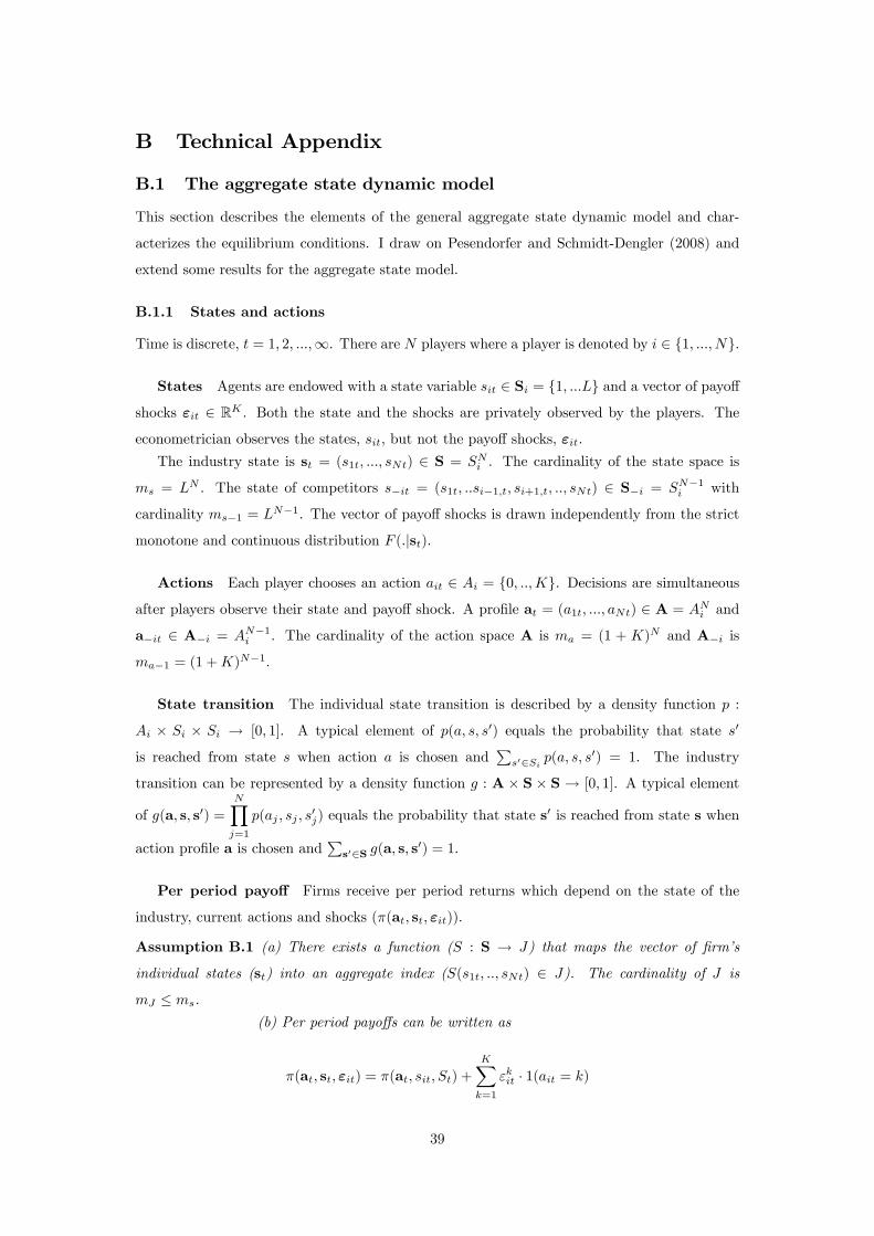
B Technical Appendix

B.1 The aggregate state dynamic model

This section describes the elements of the general aggregate state dynamic model and char-

acterizes the equilibrium conditions. I draw on Pesendorfer and Schmidt-Dengler (2008) and

extend some results for the aggregate state model.

B.1.1 States and actions

Time is discrete, t = 1; 2; :::;1. There are N players where a player is denoted by i 2 f1; :::; Ng.

States Agents are endowed with a state variable sit 2 Si = f1; :::Lg and a vector of payo¤

shocks "it 2 RK . Both the state and the shocks are privately observed by the players. The

econometrician observes the states, sit, but not the payo¤ shocks, "it.

The industry state is st = (s1t; :::; sNt) 2 S = SNi . The cardinality of the state space is

ms = LN . The state of competitors s�it = (s1t; ::si�1;t; si+1;t; ::; sNt) 2 S�i = SN�1i with

cardinality ms�1 = LN�1. The vector of payo¤ shocks is drawn independently from the strict

monotone and continuous distribution F (:jst).

Actions Each player chooses an action ait 2 Ai = f0; ::;Kg. Decisions are simultaneous

after players observe their state and payo¤ shock. A pro�le at = (a1t; :::; aNt) 2 A = ANi and

a�it 2 A�i = AN�1i . The cardinality of the action space A is ma = (1 + K)N and A�i is

ma�1 = (1 +K)N�1.

State transition The individual state transition is described by a density function p :

Ai � Si � Si ! [0; 1]. A typical element of p(a; s; s0) equals the probability that state s0

is reached from state s when action a is chosen andP

s02Si p(a; s; s0) = 1. The industry

transition can be represented by a density function g : A � S � S ! [0; 1]. A typical element

of g(a; s; s0) =NYj=1

p(aj ; sj ; s0j) equals the probability that state s

0 is reached from state s when

action pro�le a is chosen andP

s02S g(a; s; s0) = 1.

Per period payo¤ Firms receive per period returns which depend on the state of the

industry, current actions and shocks (�(at; st; "it)).

Assumption B.1 (a) There exists a function (S : S ! J) that maps the vector of �rm�s

individual states (st) into an aggregate index (S(s1t; ::; sNt) 2 J). The cardinality of J is

mJ � ms.

(b) Per period payo¤s can be written as

�(at; st; "it) = �(at; sit; St) +KXk=1

"kit � 1(ait = k)

39

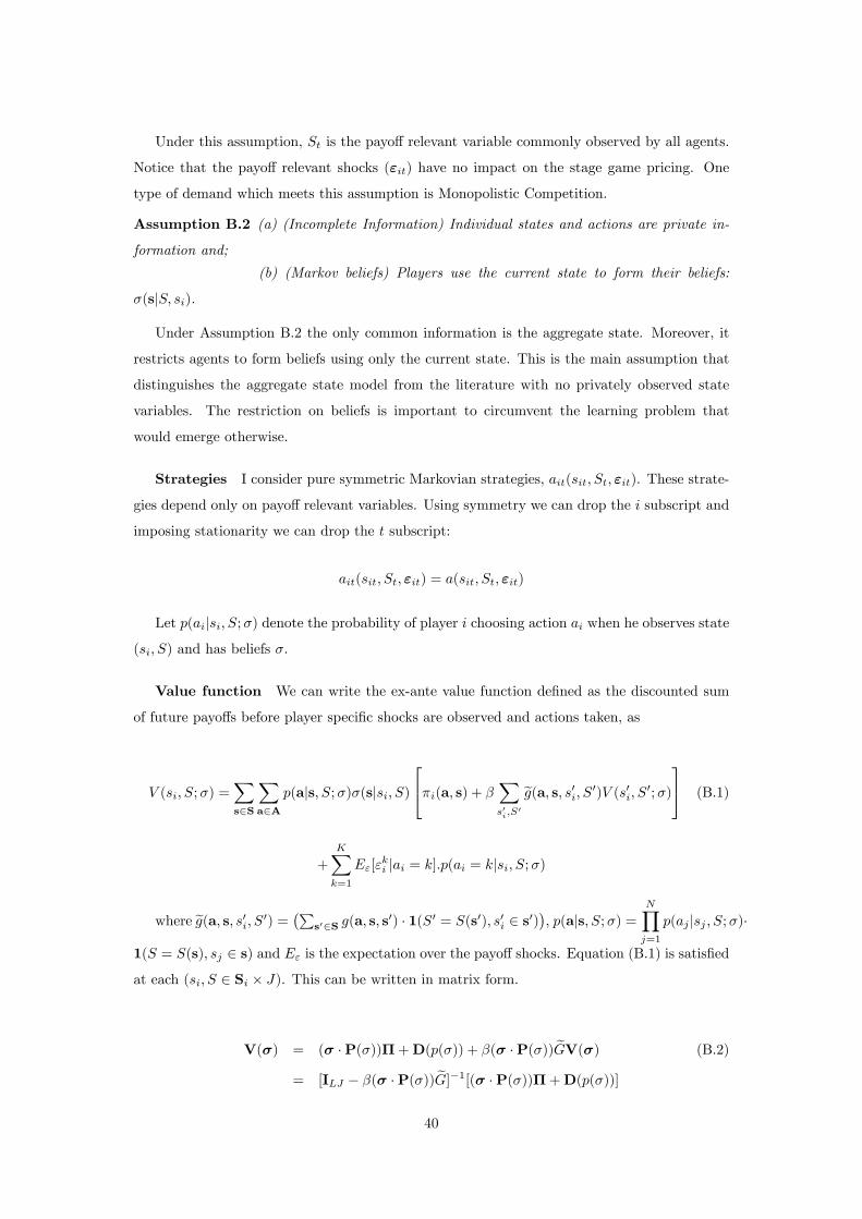
Under this assumption, St is the payo¤ relevant variable commonly observed by all agents.

Notice that the payo¤ relevant shocks ("it) have no impact on the stage game pricing. One

type of demand which meets this assumption is Monopolistic Competition.

Assumption B.2 (a) (Incomplete Information) Individual states and actions are private in-

formation and;

(b) (Markov beliefs) Players use the current state to form their beliefs:

�(sjS; si).

Under Assumption B.2 the only common information is the aggregate state. Moreover, it

restricts agents to form beliefs using only the current state. This is the main assumption that

distinguishes the aggregate state model from the literature with no privately observed state

variables. The restriction on beliefs is important to circumvent the learning problem that

would emerge otherwise.

Strategies I consider pure symmetric Markovian strategies, ait(sit; St; "it). These strate-

gies depend only on payo¤ relevant variables. Using symmetry we can drop the i subscript and

imposing stationarity we can drop the t subscript:

ait(sit; St; "it) = a(sit; St; "it)

Let p(aijsi; S;�) denote the probability of player i choosing action ai when he observes state

(si; S) and has beliefs �.

Value function We can write the ex-ante value function de�ned as the discounted sum

of future payo¤s before player speci�c shocks are observed and actions taken, as

V (si; S;�) =Xs2S

Xa2A

p(ajs; S;�)�(sjsi; S)

24�i(a; s) + �Xs0i;S

0

eg(a; s; s0i; S0)V (s0i; S0;�)35 (B.1)

+KXk=1

E"["ki jai = k]:p(ai = kjsi; S;�)

where eg(a; s; s0i; S0) = �Ps02S g(a; s; s0) � 1(S0 = S(s0); s0i 2 s0)

�, p(ajs; S;�) =

NYj=1

p(aj jsj ; S;�)�

1(S = S(s); sj 2 s) and E" is the expectation over the payo¤ shocks. Equation (B.1) is satis�ed

at each (si; S 2 Si � J). This can be written in matrix form.

V(�) = (� �P(�))�+D(p(�)) + �(� �P(�)) eGV(�) (B.2)

= [ILJ � �(� �P(�)) eG]�1[(� �P(�))�+D(p(�))]40

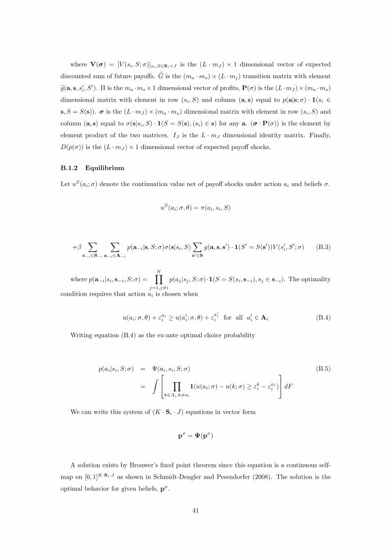
where V(�) = [V (si; S;�)]si;S2Si�J is the (L � mJ) � 1 dimensional vector of expected

discounted sum of future payo¤s. eG is the (ma �ms)� (L �mj) transition matrix with elementeg(a; s; s0i; S0). � is the ma �ms�1 dimensional vector of pro�ts, P(�) is the (L �mJ)� (ma �ms)

dimensional matrix with element in row (si; S) and column (a; s) equal to p(ajs;�) � 1(si 2

s; S = S(s)). � is the (L �mJ)� (ma �ms) dimensional matrix with element in row (si; S) and

column (a; s) equal to �(sjsi; S) � 1(S = S(s); (si) 2 s) for any a. (� �P(�)) is the element by

element product of the two matrices. IJ is the L � mJ dimensional identity matrix. Finally,

D(p(�)) is the (L �mJ)� 1 dimensional vector of expected payo¤ shocks.

B.1.2 Equilibrium

Let uS(ai;�) denote the continuation value net of payo¤ shocks under action ai and beliefs �.

uS(ai;�; �) = �(ai; si; S)

+�X

s�i2S�i

Xa�i2A�i

p(a�ijs; S;�)�(sjsi; S)Xs02S

g(a; s; s0) � 1(S0 = S(s0))V (s0i; S0;�) (B.3)

where p(a�ijsi; s�i; S;�) =NY

j=1;j 6=ip(aj jsj ; S;�) �1(S = S(si; s�i); sj 2 s�i). The optimality

condition requires that action ai is chosen when

u(ai;�; �) + "aii � u(a0i;�; �) + "

a0ii for all a0i 2 Ai (B.4)

Writing equation (B.4) as the ex-ante optimal choice probability

p(aijsi; S;�) = (ai; si; S;�) (B.5)

=

Z 24 Yk2Ai;k 6=ai

1(u(ai;�)� u(k;�) � "ki � "aii )

35 dFWe can write this system of (K � Si � J) equations in vector form

p� = (p�)

A solution exists by Brouwer�s �xed point theorem since this equation is a continuous self-

map on [0; 1]K�Si�J as shown in Schmidt-Dengler and Pesendorfer (2008). The solution is the

optimal behavior for given beliefs, p�.

41

Stationary distribution Let �(s;�) be the probability of being in state s and let the

transition be

�(s0;�) =Xs

Xa

p(ajs;�)g(a; s; s0)�(s;�) (B.6)

De�ne P� as the ms�(ms �ma) dimensional matrix consisting of p(ajs;�) in row s, columns

(a; s) and zero in the remaining columns. G is the (ma �ms) �ms dimensional matrix. Con-

vergence to a unique stationary distribution with ��(s;�) > 0 for all s 2 S occurs if P�G is a

regular matrix. We can write equation (B.6) in vector form as

��0 = P�G��

and the stationary distribution is the eigenvector (��s ), solving

(��s )�:(Ims �P�G) = 0 (B.7)

The stationary conditional distribution is

��(sjS;�) =Pr(s; Sj�)Pr(Sj�) =

Pr(Sjs;�) Pr(sj�)Pr(Sj�) (B.8)

=1(S = S(s)) � ��(s;�)Ps2S[1(S = S(s)) � �

�(s;�)]

��(sjsi; S;�) =Pr(s; si; Sj�)Pr(si; Sj�)

=1(S = S(s)))1(si 2 s)��(s;�)Ps2S[1(S = S(s); si 2 s) � �

�(s;�)]

and ��(s;�) is probability of element s 2 S occurring under the stationary distribution

(��s )�. We can write this in matrix form

��sjsi;S = �(�)

where ��sjsi;S denotes a (ms � Si � J)� 1 dimensional vector. In equilibrium, beliefs must be

consistent with optimal behavior ��sjsi;S = �

��sjsi;S = �(��sjsi;S) (B.9)

Equation (B.9) is both a necessary and su¢ cient condition for a Markov perfect equilibrium.

Theorem 1 An equilibrium exists.

Equation (B.9) gives a continuous self-map on [0; 1]ms�Si�J . Brouwer�s �xed point theorem

implies there exists (at least) a �xed point �� to the function �. This �xed point corresponds

to an equilibrium.

42