summer heat waves over western europe 1880- 2003, their ... · 2003, their change and relationship...
TRANSCRIPT

1
Summer heat waves over western Europe 1880-2003, their change and relationship to large scale forcings
P.M. Della-Marta1,2, J. Luterbacher1,3, H. von Weissenfluh1, E. Xoplaki1,3, M. Brunet4, H.
Wanner1,3.
1. Climatology and Meteorology Research Group, University of Bern, Bern, Switzerland.
2. National Climate Center, Bureau of Meteorology, Melbourne, Australia.
3. NCCR Climate, Bern, Switzerland.
4. Climate Change Research Group, University Rovira i Virgili, Tarragona, Spain. +41 (0)31 631 8868 (Work)
+41 (0)31 631 8511 (FAX)

2
Abstract:
We investigate the large scale forcing and teleconnections between atmospheric circulation (Sea Level Pressure,
SLP), Sea Surface Temperatures (SSTs), precipitation and heat wave events over western Europe using a new
dataset of 54 daily maximum temperature records. 44 of these records have been homogenised at the daily
timescale to ensure that the presence of inhomogeneities has been minimised. The daily data has been used to
create seasonal based indices of the number of heat waves and hot days. Using Canonical Correlation Analysis
(CCA), heat waves over western Europe are shown to be related to anomalous high pressure over Scandinavia
and central western Europe. We investigated the role of other forcing factors such as lagged and simultaneous
Atlantic SSTs and European precipitation, the later as a proxy for soil moisture, a known factor in strengthening
atmospheric feedback processes. The strength of the relationship between summer SLP anomalies and heat
waves is improved (from 35%) to explain around 46% of its variability when summer Atlantic and
Mediterranean SSTs and summer European precipitation anomalies are included as predictors. In agreement
with previous studies, there seems to be some predictability of heat wave events on the decadal scale from the
Atlantic Multidecadal Oscillation (AMO) and on the interannual scale using lagged precipitation deficiencies in
the Mediterranean area. A CCA using preceding winter North Atlantic SSTs and preceding January to May
Mediterranean total precipitation results in hindcast (1982-2003) correlation skill scores up to 0.55. We show
that simultaneous tropical precipitation anomalies in the Sahel region can also contribute to European heat
waves and confirm that intraseasonal variability of the African Monsoon is important in modulating atmospheric
circulation in the North Atlantic and European sector. Combining these results with the observed positive trends
in the Azores High, continental European SLP, North Atlantic SSTs and indications of a decline in European
summer precipitation then we have statistical evidence that these long-term changes are also driving increased
heat wave occurrence and it is important that the processes controlling these changes be more fully understood.
3
1 Introduction
Europe has experienced an unprecedented rate of summer warming in recent decades
(Klein Tank et al., 2005; Klein-Tank and Konnen, 2003; Luterbacher et al., 2004). In the
period 1976-1999 the annual number of periods of extreme warmth increased twice as fast as
expected from the corresponding reduction in the number of periods of extreme cold
temperatures (Klein-Tank and Konnen, 2003). Over most of Europe the increase in the mean
daily maximum temperature during the summer months has been between 0.5-1.5°C per
decade in the period 1976-1999 (Klein-Tank and Konnen, 2003). The European 2003 heat
wave was arguably one of the most significant climatic events since records began. The
extreme heat wave and drought that hit Europe in summer 2003 had enormous adverse social,
economic and environmental effects, such as the death of thousands of elderly people, the
destruction of large areas of forests by fire, and effects on water ecosystems and glaciers
(Gruber et al., 2004; Kovats et al., 2004; Schär and Jendritzky, 2004; Koppe et al., 2004;
Kovats and Koppe, 2005). According to reinsurance estimates, the drought conditions during
the summer of 2003 caused (uninsured) crop losses of around US$13 billion, while forest
fires in Portugal were responsible for an additional US$1.6 billion in damage Schär and
Jendritzky (2004). It was the unusual number of deaths during 1-15 August that caught the
news headlines (Schär and Jendritzky, 2004). Estimates based on the statistical excess over
mean mortality rates amount to between 22,000 and 35,000 heat-related deaths across Europe
as a whole (Valleron and Boumendil, 2004; Milligan, 2004; Poumadere et al., 2005). The
assessment of the environmental and health effects of the 2003 and previous heat-waves has
highlighted a number of knowledge gaps and problems in public health responses. To date,
heat waves have not been considered a serious risk to human health with epidemic potential
in the European Region (Kovats and Koppe, 2005). Reducing the health impact of future heat
waves requires addressing fundamental questions, such as whether heat waves can be
predicted, detected and whether their impacts can be mitigated. From a public health
viewpoint some countries are much more vulnerable than others such as those in
midcontinental areas where seasonal and diurnal ranges of temperatures are greater (Koppe
et al., 2004; Kovats and Koppe, 2005). Heat waves are believed to become more frequent,
more intense and longer lasting with climate change (Meehl and Tebaldi, 2004; Schär et al.,
2004; Beniston, 2004; Stott et al., 2004; Huth et al., 2000). The sobering science of Stott et al.
(2004) show that there is a detectable man-made influence on the frequency of extremely

4
warm climatic events and it is very likely that the European heat wave of 2003 was in part
attributable to human activities. Their study shows that there has been at least a doubling in
the risk of the mean 2003 summer European temperature being exceeded. The ageing of the
European population, together with the potential effects of climate change may exacerbate
the threats to human health posed by thermal stress in the future (Koppe et al., 2004; Kovats
and Koppe, 2005). Recently, in the meteorological community there have been many studies
looking more closely at the 2003 event in the context of past climate variability (Chuine
et al., 2004; Schär et al., 2004; Luterbacher et al., 2004) and future changes in the frequency
of heat waves (Meehl and Tebaldi, 2004; Schär et al., 2004; Beniston, 2004; Stott et al., 2004;
Fink et al., 2004). Other studies have focused on the interpretation of weather diagnostics of
the 2003 heat wave (Black et al., 2004; Trigo et al., 2005; Fink et al., 2004; Ogi et al., 2005).
A growing number of studies have looked at the mechanisms that contribute to the formation
of such extreme events such as Sutton and Hodson (2005) who attribute long-term variability
of European summer average temperature to a mode of SSTs called the Atlantic Multidecadal
Oscillation (Enfield et al., 2001). Cassou et al. (2005) show that there is a significant
influence from the tropical Atlantic region on the formation of Rossby wave trains and
atmospheric blocking conditions necessary to have anomalous summer heat waves. Vautard
et al. (2006) show that rainfall deficiencies in the preceding winter Mediterranean
precipitation have a discernable effect on the frequency of Heat Waves (HWs) through
northward transport of latent heat fluxes. Nakamura et al. (2005) use the Earth simulator
forced with daily observed SSTs one month before the event in three different regions of the
North Atlantic. They show that high frequency wave forcing in the vicinity of the Gulf
Stream was an important factor in maintaining blocking over western Europe.
These studies are part of a global effort to focus climate research on the nature of weather
extremes and their impacts on society. Since the Intergovernmental Panel on Climate Change
(IPCC, 2001) third assessment report there has been a concerted effort by National
Meteorological Services to make available long, high-quality climate records in order to
assess the changes and variability in daily climate extremes around the world (Alexander
et al., 2006; Klein-Tank and Konnen, 2003; Collins et al., 2000; Zhang et al., 2005; Manton
et al., 2001; Peterson et al., 2002; Frich et al., 2002). Many of these studies on climate
extremes have focused on their long-term changes over the maximum possible period for
which reliable daily data exist. Another major focus of climate research has been the use of
synoptic climatology (Hess and Brezowsky, 1977; Lamb, 1972; Yarnal, 1993) analysis
techniques to investigate how the large-scale synoptic weather patterns affect the frequency
5
and trends in extremes (Haylock and Goodess, 2004; Domonkos et al., 2003; Xoplaki et al.,
2003).
This study aims to build a more complete database of high quality daily resolved station data
with a detailed look at the variability and trends in the frequency of heat waves across Europe
over the last 124 years and relate these phenomena with atmospheric circulation data, SSTs
and other possible forcing factors or covariates. Inherent in our aim is to verify possible
mechanisms of European heat wave formation given a more complete and rigorous
observational dataset.
Our definition of a heat wave is similar to other studies such as Collins et al. (2000). We use
daily maximum temperature to count the frequency of extended periods of extreme
temperature. Extreme temperature is defined as an temperature above a percentile threshold
to ensure that the heat wave index is applicable to different climatological regions.
This paper starts with a description of the data and methods used in the study. This section
covers the source and homogeneity issues of the data. We discuss Canonical Correlation
Analysis (CCA), the main statistical method used in the paper. The results of the analysis are
presented, discussed and concluded in the following parts.
2 Data and Methods
In this section we describe the various datasets and indices used in this study. We have split
this section into Predictor and Predictand subsections to help clarify which data have been
used for what purpose. The predictor data used in this study is not always strictly a true
predictor in the sense that it could be used to forecast in time the occurrence of heat waves.
The label is simply used to clarify which data are presumed to be the independent variables
versus the dependant variables.
2.1 Predictor Data
Sea Level Pressure (SLP) Data
The SLP dataset used in this study was created as part of a collaborative European project
named EMULATE (European and North Atlantic daily to MULtidecadal climATE
variability, http://www.cru.uea.ac.uk/cru/projects/emulate/). It is a daily resolution gridded
dataset that covers the North Atlantic and European area from 70°W to 50°E and 25°N to

6
70°N on a 5°× 5° grid. Details of this dataset including the quantity, quality and methods of
reconstruction can be found in Ansell et al. (2005). The dataset combines 82 daily land
station series and ship observations. The land station series and ship observations have been
corrected for elevation and diurnal pressure variations as well as inhomogeneities caused by
instrument changes and/or location.
Sea Surface Temperature Data
Sea Surface Temperature (SST) has been shown to have predictive skill in forecasting the
boreal winter North Atlantic Oscillation (NAO) (Rodwell et al., 1999) although the effects of
this sea-air coupling are more noticeable at decadal timescales (Sutton and Hodson, 2005). In
fact Ratcliffe and Murray (1970) show significant but time varying influence of SSTs on the
North-Atlantic circulation. Paeth et al. (2003) studied the influence of SSTs on the annual
NAO and conclude that the SST forcing is barely noticeable at interannual timescales but is
highly significant at decadal timescales. Mosedale et al. (2005) showed that the air-sea
coupling process over the North Atlantic is detectable at daily timescales in a coupled
atmosphere-ocean GCM. Colman (1997) shows that January and February North-Atlantic
SST can be used as a predictor of summer, July-August, Central England Temperature (CET)
with a correlation skill score of around 0.5. Since it is clear that SSTs play a role in
modulating atmospheric circulation and climate, the global monthly Sea Surface Temperature
dataset of Smith and Reynolds (2004) going back to 1854 was used as a potentially important
variable in explaining the frequency of heat waves over Europe.
Precipitation Data
Many authors have cited the importance that low soil moisture played in attributing cause to
the 2003 heat wave (Schär et al., 2004; Black et al., 2004; Fink et al., 2004). Others have
shown through modelling studies the increased likelihood of extreme temperatures and heat
waves associated with drier soil conditions (Brabson et al., 2005; Findell and Delworth, 2005;
Ferranti and Viterbo, 2006; Schär et al., 1999) To first order the amount of evapotranspiration
is dependant on precipitation (Ferranti and Viterbo, 2006; Schär et al., 1999) and since the
authors are unaware of any comprehensive soil moisture dataset extending back to 1880 we
decided to see if the preceding winter or spring precipitation was a potential predictor of the
severity of heat waves. Here we have used the global gridded monthly dataset of Mitchell and
Jones (2005) called CRU TS 2.1. This dataset currently ends in 2002 so to include 2003 we

7
used data from the Climate Prediction Center (CPC) Merged Analysis of Precipitation
(Huffman et al., 1997).
2.2 Predictand Data
Station Based Temperature data
The station based data are a collection of daily resolution long-term records from around
Europe. They are primarily a combination of two datasets, the European Climate Assessment
database (Klein-Tank et al., 2002; Wijngaard et al., 2003; Klein-Tank, 2002) and the
EMULATE database (Moberg et al., 2006). The database contains daily minimum, mean and
maximum temperature and daily total rainfall of varying quality and continuity. However,
only records that had met more rigorous continuity, quality control and homogeneity criteria
were used in this study. The daily records needed to have at least 70% complete and non-
missing data over the analysis period, 1880-2003 with the additional constraint that no
missing values be present in the last five years of the analysis period. The latter criteria
helped to minimise the effects of missing data on the trend analysis and helped to reduce
biases in the CCA associated with missing data. Records were carefully screened for
inconsistencies including, maximum and minimum logic tests and investigation of outliers
(Moberg et al., 2006). We decided to check the homogeneity of these records in more detail
and where possible homogenise the daily records ourselves. Of the 178 stations in the
database (Moberg et al., 2006) only 54 records met these criteria. However, even if a station
was not included in the final dataset (54 stations), the other stations in the database were
useful to help assess the homogeneity and in some cases homogenise daily maximum
temperature.
Homogenisation of the daily maximum temperature records
Each of the 54 stations used in the analysis can be classified as either homogenised or non-
homogenised and each of the homogenised records have varying quality of homogeneity
depending on the type of homogenisation method applied. Below is an itemised list of the
homogenisation categories:
• HOM method ++ : The Higher Order Moments (HOM) method of Della-Marta and
Wanner (2005) was used with high quality metadata detailing the break points and the

8
magnitude of adjustments to monthly mean maximum temperature for both the
candidate and reference stations.
• HOM method +−: Uses the HOM method with a combination of high quality
metadata detailing the break points and the magnitude of adjustments to monthly
mean maximum temperature and the results of a Relative Homogeneity Test (RHTest)
for either the candidate or reference stations.
• HOM method −−: Uses the HOM method with limited metadata and only the results
of the RHTest to provide information about possible break points.
• RHTest only: Mean adjustments to the daily maximum temperature series were
derived from the results of the RHTest applied to monthly and annual maximum
temperature data using limited or no metadata.
• Other: The daily maximum series was homogenised previously by another study. See
the references in table 1 for details of the methods used.
The order of the first four items in the list above denotes a natural progression in the level of
quality we believe the final homogenised series has. It is difficult to assess the quality of the
records in the "Other" category since a direct comparison of methods was not made, however
most of these studies have applied the monthly adjustments calculated from a relative
homogeneity test to the daily values. Each station's basic metadata and the level of
homogenisation applied to the series is detailed in table 1.
As a first step in identifying possibly erroneous stations the homogeneity assessment data
from Wijngaard et al. (2003) were used since many of the stations in the EMULATE
database come from the ECA (European Climate Assessment). We also used the results from
previous studies to help identify potentially inhomogeneous stations and to gather metadata.
Böhm et al. (2001) and Auer et al. (2005) focus on the homogeneity of temperature
measurements over the Alpine region. They used a variety of techniques to identify and
adjust their monthly and annual data including the MASH technique (Szentimrey, 1999) and
those of Auer et al. (1999) and Mestre (1999). Begert et al. (2005) have identified many
inhomogeneities in the Swiss daily mean temperature data whereas Herzog and Müller-
Westermeier (1998) have investigated German monthly mean temperature data. Parker and
Horton (2005) have homogenised daily maximum and minimum temperature for the Central
England Temperature (CET) series. Moberg et al. (2002), Moberg and Bergström (1997) and
Bergström and Moberg (2002) looked closely at the daily mean Stockholm and Uppsala
temperature series. Demarée et al. (2002) has investigated the homogeneity of daily mean

9
temperature of the Central Belgium Temperature (CBT). Brunet et al. (2006b) have recently
homogenised daily maximum and minimum temperature for 22 long-term Spanish series and
analysed their long-term trends and variability (Brunet et al., 2006a). Butler et al. (2005)
investigated the homogeneity of the Armagh daily maximum and minimum temperature.
Metadata and monthly adjustments for Paris-Mountsouris record were provided by Olivier
Mestre (2005 pers. comms.). The homogeneity adjustments were based on the method
presented in Caussinus and Mestre (2004). Other authors have homogenised daily mean
temperature series (e.g. Maugeri et al., 2002) however these series could not be used for the
sake of consistency with the maximum temperature records used in this study.
Where possible we used the method of Della-Marta and Wanner (2005) to homogenise the
daily maximum temperature used in this analysis. The method presented in this paper can
adjust both the mean and the higher order moments (i.e. variance and skewness) of a daily
temperature record. The most critical requirement for this method to work is the presence of a
highly correlated reference station which has homogeneous sub-periods overlapping the date
of the inhomogeneity in the candidate station. Knowing at which time inhomogeneities in the
data occur is a difficult task, so we limited our efforts of daily homogenisation to stations
where we could either obtain reliable metadata (HOM method ++ or HOM method +−) in
collaboration with the data providers listed in the acknowledgements (or previous studies
listed in table 1) or where we were confident that the RHTest (detailed below) was providing
reliable estimates of break points. The countries where this was possible were (some or all
stations): Austria, Czech Republic, Germany, The Netherlands, Portugal, Sweden,
Switzerland, United Kingdom. We homogenised a total of 25 stations using the HOM
method. See table 1 for the details of each station and Della-Marta and Wanner (2005) for
more details on the method. Detailed results from the application of the HOM method
showed (not shown) that many stations needed adjustments not only to their mean but also
their variance and skewness characteristics. Most methods of daily homogenisation only
explicitly homogenise the mean, however Della-Marta and Wanner (2005) show that
inhomogeneities in the higher order moments can also be present in daily series which need
to be corrected.
Where metadata on the break points (inhomogeneities) in candidate and reference stations
were limited we used a RHTest to try and determine their occurrence. A number of different
techniques exist to identify inhomogeneities and an overview of the variety of tests is given
by Peterson et al. (1998). However we checked the homogeneity of annual and monthly
10
averaged data using a two-phase regression model used by Easterling and Peterson (1995)
among others and then subsequently improved by Lund and Reeves (2002) and modified by
Wang (2003). Wang (2003) uses a slightly simplified two-phase regression model compared
to Lund and Reeves (2002) which allows the two-phase model to have a common trend
parameter instead of two different trend parameters. Lund and Reeves (2002) which allows
the two-phase model to have a common trend parameter instead of two different trend
parameters.
This model known as the RHTest (Wang, 2003), was applied to both the raw anomalies (with
respect to the overall mean) of the candidate station and a difference series calculated as the
difference between the candidate series and a reference series created from a weighted
average of surrounding station series. The method to create the weighted reference series
follows Della-Marta et al. (2004) where a weighted reference series is created from stations
that have at least ten years of annual average maximum temperature data and have a
significant correlation (p-value≤0.05) with the candidate series above 0.6 and the inter-station
separation is less than six degrees along a great circle. See Della-Marta et al. (2004) for more
details.
A comparison of the number of inhomogeneities (not shown) detected using the difference
series compared to those detected when using the candidate series only with known dates of
potential inhomogeneities (metadata) confirms that the relative or difference test in general
produces more reliable results given a suitably reliable reference series (e.g. Della-Marta
et al., 2004; Begert et al., 2005).
Extreme temperature indices
The extreme indices detailed below are based on daily data, however since most of the
indices are frequency or counting based they have been summed or averaged to create
seasonal time resolution indices. The objective of these indices is to provide information on
the occurrence and frequency of heat waves and extremely hot temperatures. Primarily these
indices are aimed at the climatological community for assessment of climate change and
long-term variability, and secondly to provide information which is useful to epidemiologists
investigating the morbidity and mortality that they cause. Since the public health effects of
heat waves are complex and outside the scope of this paper we will not discuss mortality or
morbidity related statistics or define a heat wave index that is the most appropriate to these
kinds of investigations. Meteorologically, the essential component of a heat wave are

11
sustained duration of extremely high temperatures. Several approaches can be used to define
a heat wave, based on an absolute or a relative threshold of weather variables or as a
combination of both. Robinson (2001) gives an overview of the U.S. National Weather
Service heat wave index. A survey of the meteorological services in Europe (Koppe et al.,
2004; Kovats and Koppe, 2005) showed that an operational definition of a heat wave has a
varying definition but essentially is based on the following elements.
• Air temperature threshold
• Air temperature threshold and a minimum duration
• Indices based on a combination of air temperature and relative humidity
Due to the lack of any long-term humidity database for Europe over the period of
investigation we decided to base our definition of a heat wave on air temperature and a
measure of duration. The temperature threshold in the indices varies according to each
stations Probability Distribution Function (PDF) to make the definition of the heat wave
relative to the local climate. Generally the temperature thresholds used in Europe have a
north-south and a west-east gradient. The index names and definitions are summarised below.
• Heat waves (HW): Defined as the number of consecutive three day periods in summer
that exceed the long-term 80th percentile of daily maximum temperature (calculated
using daily data from 1906-2004).
• Hot Days (HD): Defined as percent of time in a season where the daily maximum
temperature exceeds the long-term 90th percentile (calculated using daily data from
1906-2004).
• Average Maximum Temperature (TXAV): The average seasonal maximum
temperature.
The 80th percentile was chosen for the HW index so that each seasonal count had a higher
chance of not containing zero heat waves, remembering that we need at least three
consecutive days above each stations' threshold. If the 95th percentile was chosen we could
only expect on average around five days above this threshold per season whereas the 80th
percentile offers around eighteen days on average. Clearly then, the number of consecutive
three day periods being captured using the 80th percentile is higher. A follow on effect of a
seasonal HW count being zero often would be that the statistics of the CCA would be
possibly unreliable due to a very heavy-tailed and skewed distribution of the seasonal
extreme index. The HD index was chosen for its simplicity and the ability to be able to
compare it easily with other studies on changes in extreme temperature as well as giving an
12
indication of the frequency of more extreme temperatures . The summer average maximum
temperature indices were included to allow a comparison between changes in the mean and
extremes.
2.3 Canonical Correlation Analysis
CCA is a statistical technique that relates many predictor variables to many predictand
variables in such a way that the correlation between the two datasets is maximised (e.g. von
Storch and Zwiers, 1999; Wilks, 1995). It has been used extensively throughout the
meteorological and climatological literature (e.g. Nicholls, 1987; Haylock and Goodess,
2004; Xoplaki et al., 2003). Cherry (1996) highlight the need for caution in interpreting the
results of CCA. Importantly they note that even spatially and temporally uncorrelated data
can produce high canonical correlations between variables. The problem of spurious coupled
modes is increased when sample sizes are small, when the data is autocorrelated or coupled
modes are weak. As with any parametric statistical analysis, there are inherit assumptions that
are often neglected as being important. CCA is based on the axioms of correlation analysis.
Correlation coefficients between two data sets (and their significance) are affected by non-
stationarities in the data such as trends and autocorrelation (Chatfield, 1996). The predictor
and predictand data were all standardised before the CCA was performed, giving equal
weight to all gridpoints and station data points and converting the data into anomalies with
respect to the entire analysis period (1880-2003, and 1901-2003 for precipitation data). We
also explored the differences between CCA models with trends remaining in the data and
with all series detrended. When determining the predictive skill of a model we always
detrended the data first, however if our goal was to simply explore possible relationships
between variables we did not remove the trend. The preprocessing of the data before CCA
included dimensional reduction using Principal Component Analysis (PCA) retaining the
significant number of Principle Components (PCs) using Rule N criteria (Preisendorfer,
1988). One thousand synthetic datasets were created and the significant number of principal
components assessed at the 0.05 significance level, see Haylock and Goodess (2004) for
more details on the preprocessing and CCA methodology. This process had the added benefit
of removing the effects of collinearity and spatial dependence between variables. The number
of significant PCs for each variable set the upper limit to the number that could be used in the
subsequent CCA analysis. This may not be the optimal number of PCs to use in the CCA,
since CCA is analogous to a multiple linear regression where it is easy to overfit the model
by including too many predictor variables. To account for this problem we performed a CCA
13
for every combination of predictor PCs and predictand PCs and performed a cross-validation
procedure taking one year out of the CCA at one time and assessing the prediction errors as
the mean Spearman rank correlation skill score. Most of the time this resulted in the number
of PCs taken as predictors or predictands being less than the upper limit number of significant
PCs for the predictor and predictand. In the case where more than one predictor variable was
used the significant PCs from each predictor variable were combined and then PCA was
performed on this combined PC representation of the multiple predictors. The PCs from this
second-level PCA were cross-validated in the same way as described above to determine the
number of PCs to be used in the CCA analysis. We tried to minimise the possible over-
interpretation of CCA results by also performing a hindcast for each CCA where the model
was trained on the first 70% of the data and a validation performed on the remaining years. A
number of measures were used to assess the fit of the CCA model to the validation data.
These included the Spearman rank correlation, Root Mean Squared Error (RMSE) as well as
an Absolute Mean Bias (AMB).
3 Results
In this section we present the results of trend analysis of selected predictor and predictands
and CCA analysis between SLP, North Atlantic SSTs, Precipitation from various
geographical regions and the frequency of summer HWs each station. In some experiments
more than one predictor was used which we refer to as multiple predictor CCAs. A summary
of the predictor and predictand data sets is shown in table 2. This table shows the abbreviated
name used to refer to each predictor or predictand, the season over which the variable was
averaged, the geographical domain and the number of significant principle components that
were determined using the monte-carlo techniques detailed in section 2.3.
3.1 Long-term trends in the frequency of extreme temperature indices, SLP, SST and precipitation
Figure 1 shows that the majority of stations used in this analysis have a positive trend in the
occurrence of HWs from 1880-2003. Around two thirds of the trends are statistically
significant at the 95% confidence level. The trend significance (not shown) was determined
using the non-parametric Kendall Tau test (Press et al., 1996). A non-parametric test was
used since the distribution of the HW is usually long-tailed and not Gaussian. Sometimes the
trend shown on the plot has not been calculated over the whole period (See table 1 for details

14
on the starting dates of each record). Trends of up to 0.53 HWs per decade were found for
Madrid in Spain. The largest trends have been found over the Iberian peninsula and in central
western Europe. Incidently this is where we also have the most confidence in our data (See
table 1 for an overview on the quality and homogeneity of each station series). According to
Brunet et al. (2006a), a general and highly significant warming on an annual and a seasonal
basis has been observed during 1850-2003 over mainland Spain. The most remarkable feature
of the Spanish long-term temperature change has been the unprecedented and strong rise in
temperatures observed since 1973 on an annual basis associated with larger increases for
spring and summer temperatures compared to those for winter and autumn. There is only one
negative trend (-0.01 HWs per decade) in the occurrence of HWs at Lisboa-Geofisica in
Portugal. Both the highest trends of the other indices, HDs and TXAV, occurred in Spain
with 1.5 percent of time per decade at Madrid and 0.27°C per decade at Valladolid
respectively. Generally the spatial distribution of the trends and their statistical significance
of these indices resembles the distribution of the HW index trends shown in figure 1 (not
shown).
Generally the summer climate of Europe and the Azores region of the North-Atlantic has
experienced an increase in average JJA mean sea-level pressure from 1880-2003 (Fig. 2),
although the regions of statistically significant trends are not widespread and occur in isolated
regions. Significant positive trends of up to 0.15 hPa per decade were found in the Azores
region whereas significant negative trends of up to 0.10 hPa per decade were found in the
Icelandic low region.
Summer SSTs in the North Atlantic region (SSTNA) have become warmer over most of the
domain. Close to the coastline of Western Europe and in the Mediterranean (Fig. 3), trends up
to 0.12°C per decade have been found whereas SSTs have decreased in the region south of
Greenland although only significantly in isolated regions. The regions with the highest
statistically significant positive trends lie east of Newfoundland and around the Portuguese
coast and the British Isles.
There has been a general drying trend in precipitation across western Europe (Fig. 4) in
agreement with Pal et al. (2004). Isolated yet numerous areas of statistically significant
negative trends are shown. Significant positive trends exist over the northwest Iberian
peninsula.

15
3.2 Simultaneous SLP as a predictor of heat waves
Black et al. (2004) and Luterbacher et al. (2004) showed the importance of persistent
anticyclonic conditions over Europe contributing to the 2003 heat wave. We find that there
are two major modes of SLP variability associated with summer HWs (in agreement with the
cluster analysis derived patterns of Cassou et al. (2005) called Blocking and Atlantic Low and
CCA derived patterns of Xoplaki et al. (2003)). The first CCA mode (Fig. 5a) shows that
strong positive anomalies of SLP over the Scandinavian region are associated with
anomalously high frequency of HWs (Fig. 5b) over northern and central western Europe and
weak negative HW anomalies over the Iberian peninsula. This pattern also resembles the
summer NAO described in Hurrell and Folland (2002) who showed that the SLP in the
northeast Atlantic was anomalously high from the mid 1960s to the mid 1980s. The canonical
score series (Fig. 5c) show the time evolution of the CCA loadings. The dashed line shows
the canonical score associated with HWs and the solid line shows the canonical score
associated with the SLP. The correlation between the two score series of the first CCA is 0.8
(summarised in table 3) which is high. Notably the summers of 1997, 1976, 1959, 1947 and
1911 show a high score on this CCA mode (dashed line in figure 5c). The 1976 event was at
the time thought to be unprecedented by Ratcliffe (1976) in the previous 250 years. A
detailed overview of the event affecting the British Isles can be found in Shaw (1977). As we
will discuss below this was also a very dry summer. The first CCA explains an average of
17% of HW variability.
The second CCA loading pattern shown in figure 6a resembles a stationary wave pattern with
anomalously low SLP over central North Atlantic, positive anomalies over western Europe
and negative anomalies over eastern Europe. This CCA only explains 8% of the total HW
variability over the domain, however this CCA mode has a high HW score value associated
with the 2003 heat wave (figure 6c black curve) indicating that this pattern (Fig. 6a,b) was
important in the development of the 2003 event. Notice however that there is a large
difference between the solid and the dashed curve in figure 6c which indicates that the CCA
predictor (SLP) underestimated the observed within CCA HW variability. Combined all four
CCAs explain a modest 32% (Table 3) showing that other factors apart from atmospheric
circulation are important for the formation of HW events.
16
3.3 Simultaneous and lagged SST as a predictor of heat waves
Primarily there are two modes of SSTNA variability that are coincident with summer HWs
which for the sake of brevity are not shown but are described below. The first shows that
anomalous warm (cold) SSTs around the North and Baltic seas extending southward along
the Bay of Biscay and the western coast of the Iberian peninsula and westward to the Azores
are linked with anomalously high (low) frequency of HWs across western Europe with
highest loadings in central western Europe. The second SSTNA CCA shows a dipole
structure with cool (warm) Baltic and North Seas with a warm (cool) Mediterranean. A
summary of the total explained variance of the SSTNA/HW CCA is shown in table 3. Notice
that the explained variance is similar to using SLP as a predictor of HWs at 34%.
Lagged SSTNA in the months of DJF and MAM preceding JJA HWs do not show (see table
3) particularly promising lead skill. Generally anomalously warm SSTs in MAM and DJF
over the whole SSTNA domain except a cooler area east of Newfoundland, or anomalously
warm SSTs in the Baltic and North Seas are associated with higher HW occurrence in
summer. Only around 4% - 5% of HW variability can be explained by SSTNA in MAM or
DJF. The hindcast Spearman rank skill score shows widespread weakly positive correlations
except in central western Europe where correlations around 0.5 indicate that around 25% of
HW occurrence can be predicted by preceding SSTNA (not shown).
We repeated this analysis to predict JJA TXAV (not shown) in order to try and verify the
findings of Colman (1997) who show a correlation skill score of 0.5 (≈25% exp. var.)
between Central England Temperature series and preceding winter (January-February) SSTs.
Our CCA between the first four DJF SSTNA PCs and the first four JJA TXAV does not
produce a correlation skill as high as Colman (1997) for Central England Temperature (CET)
with only a hindcast (1966-2003) Spearman rank correlation skill score of 0.09. However
there are correlations as high as 0.4 in parts of Spain and western Europe (excluding the
British Isles). Here we have not reproduced their experiment exactly. Differences such as the
number of PCs retained and the winters months taken as predictors, as well as the statistical
method could be responsible. However in summary we find a weak but significant signal of
winter SSTs affecting the summer average temperature and frequency of HWs over western
European.

17
The Atlantic Multidecadal Oscillation
Many authors have suggested that potential predictability of climate can be found in the
decadal and longer cycles of SSTs (e.g. Rodwell et al., 1999). Here we find evidence
supporting the analysis of Sutton and Hodson (2005) that the occurrence of warmer than
average temperatures over Europe are related to long term changes in the Atlantic
Multidecadal Oscillation (AMO) (Enfield et al., 2001). The AMO is believed to be caused by
the North-Atlantic thermohaline circulation (Knight et al., 2005). The correlation between the
LOESS smoothed (Cleveland and Devlin, 1988) HWPC1 score series and the AMO (see
table 2 for the definitions) shown in figure 7a is 0.8. The significance is hard to determine
since the effective number of degrees of freedom is around 2. Figure 7b, shows the loading
pattern associated with HWPC1. According to this PC the western European domain is under
the influence of anomalously high or low frequency of HWs. High occurrence of HWs
between 1880-1905, 1925-1950 and 1990-2003 periods is coincident with anomalously high
SSTs in the region defined by the AMO. Although this analysis does not provide a causal link
between the long term variations in North Atlantic SSTs it is interesting to compare them
since for the first time such a long-term analysis of European HWs has been performed. It is
tempting to extrapolate from figure 7a that there is a phase lag between the AMO series and
the HWPC1 since the peaks (troughs) of the HWPC1 series tend to lag the AMO peaks
(troughs) by approximately five years. Could the atmosphere retain and react to an ocean
forcing from five years earlier? It is certainly an interesting question that can only be
answered by many forced and unforced complex model simulations.
3.4 Simultaneous and lagged precipitation as a predictor of heat waves
Schär et al. (1999) show the importance of summertime precipitation and soil moisture
feedback processes as a significant factor in the probability of severe and long lasting rainfall
deficiencies over Europe. Ratcliffe (1977) suggested that this mechanism was partly
responsible for the severity of the 1975/76 drought affecting western Europe and the British
Isles. Heat waves are also related to soil moisture deficiencies (Brabson et al., 2005; Ferranti
and Viterbo, 2006) thus we investigated the role of PRECWE (see table 2) summer
precipitation on the occurrence of HWs.
In the first CCA (not shown), anomalously dry (wet) western central and northern European
summers are associated with a higher frequency of HWs in those areas, whereas there is little
association over the Alps and anomalously higher (lower) summer precipitation over the

18
Iberian peninsula is associated with fewer (more) HWs. The years 1975/1976 and 1982 stand
out as being extreme years in this CCA. The 1976 drought was discussed by Miles (1977)
and Ratcliffe (1977) who associated the anomalous conditions with colder than average North
Pacific SSTs, lack of cyclonic circulation types over the British Isles and western Europe and
feedback reactions with the Atlantic SSTs.
The second CCA shows that strong negative PRECWE anomalies over most of central
western Europe are associated with anomalously high frequency of HWs. Other notable
extremes in the CCA score series are the summer of 1911 where widespread HWs were
accompanied by drought conditions (see Burt (2004) for an overview of the event in the
U.K.) and 1947 and 1949. Again the explained variance of these two modes is only a modest
13% and 12% each and a total of 30% explained variance (table 3).
Lagged and simultaneous Mediterranean precipitation
Recently Vautard et al. (2006) documented the link between preceding winter precipitation in
the Mediterranean region as a possible useful predictor of the occurrence of HWs in Europe.
However since their analysis only presents a correlation and not a rigorously cross-validated
model, over the last 50 years, we decided to perform this analysis over a longer period which
our data affords us and using the CCA model framework. Figure 8 shows the first canonical
patterns and scores between PRECME and HWs. The first canonical pattern shows that
strong negative anomalies (canonical correlation between -0.5 and -0.7) of precipitation over
the PRECME area are linked to a higher frequency of HWs over central western Europe and
the Iberian Peninsula. However the overall canonical correlation is weak (0.42) and overall
this CCA only explains 6% of HW variability. Interestingly the hindcast (Fig. 8d) results
reveals significant skill in central and western Europe with correlation skill scores in the
order of 0.3 and up to 0.5 indicating that around 10-20% of HW occurrence can be explained
using this regions lagged precipitation. We used the same predictor, PRECME to estimate the
index TXAV and found that the hindcast Spearman rank skill score indicated that between
15-25% of the average summer maximum temperature could be explained.
Simultaneous tropical precipitation
Cassou et al. (2005) used a Global Climate Model (GCM) to show that anomalous diabatic
heating in the tropical Atlantic and anomalous northern South American and Sahel
precipitation can help produce a diabatically induced Rossby wave train that originates in the
Caribbean and helps maintain blocking stationary waves over Europe. They link the

19
occurrence of two circulation modes (described above) to anomalous occurrence of extremely
warm days over France. They point out the importance of seasonally varying position of
diabatic heating in the tropical Atlantic and that several mechanisms can contribute to hot
conditions over Europe within the summer season. In June they suggest that teleconnections
between 500hPa height anomalies over Europe are strongest with anomalously high
precipitation over South America north of the equator. In August the teleconnection is more
strongly linked to the northward movement of the African monsoon with high precipitation in
the Sahel region. Again, we tried to replicate their findings over the longer period of data we
have available, using precipitation as a proxy for diabatic heating. The regions we chose were
those shown in Cassou et al. (2005) supplementary figure 4. Using PRECNSA, PRECBR and
PRECTA (see table 2) as predictors of JJA HWs we find that the tropical precipitation
influence is rather small (total of 6% explained HW variance) and when the hindcast is
applied we get weakly positive Spearman rank correlation skill scores over most of the
domain (0.3-0.5) and very weak skill scores over the Alpine region. When we included SLP
as an additional predictor we improved both the overall explained variance (38%, table 3) and
the hindcast Spearman rank correlation skill score to be positive over the western half of the
domain (generally between 0.3 and 0.6). The CCAs (not shown) show that HWs can be
associated with different combinations of precipitation anomalies in the tropics. The first
CCA shows that near normal conditions in PRECNSA and PRECBR in June and a slightly
drier than average Sahel in August is associated with an SLP pattern similar to that shown in
figure 5a and more HWs in the north of western Europe. The second CCA shows
anomalously dry conditions in both PRECNSA and PRECBR in June and mixed anomalously
wet and dry PRECSH in August is associated with an SLP pattern like that shown in figure
6a and anomalously more HWs over most of western Europe. Hence using this model we
cannot reproduce the teleconnection of Cassou et al. (2005). Of course these modes could be
a statistical artifact of the CCA and caution must be taken in interpreting such patterns since
the overall skill of the model is weak. This result prompted us to look closer at only the
influence of Sahelian precipitation and it's connections with SLP and HWs. Since Cassou
et al. (2005) claim that intraseasonal variability of tropical heating is important we used June,
July and August Sahelian precipitation as well as JJA SLP as predictors of JJA HWs. The
first two CCAs are shown in figures 9 and 10. The first CCA explains 16% and indicates that
anomalously dry (wet) conditions for each month, June, July and August in the Sahel is
associated with anomalously high (low) SLP over the north of Western Europe and
Scandinavia resulting in anomalously more (less) HWs in this region. This CCA mode does
20
not seem to be an artifact of the method since a simple correlation between total JJA
PRECSH and the second principle component of JJA HWs (this PC's loading pattern looks
similar to the CCA loading pattern in Fig. 9d) is −0.2, although weak it is statistically
significant at the 95% confidence level. The second CCA explains approximately 24% and
indicates that anomalously high June and August and normal July precipitation in the Sahel is
associated with anomalously high (low) SLP over central Western Europe and resulting in
anomalously more (less) HWs over most of the domain. Clearly the intraseasonal variability
of African monsoon and Sahelian rainfall plays an important part in the modulation of
atmospheric circulation in the North Atlantic and the European region. Summary results in
table 3 indicate that the total explained variance of HWs is higher when Sahelian
precipitation is included as a predictor along with SLP, however the µhindcast is clearly not as
good as using simply SLP as a predictor.
3.5 Multiple simultaneous predictors of heat waves
In the experiments presented earlier between simultaneous SLP, SSTNA and PRECWE, the
predictors were all highly correlated with HWs (based on the results in table 3 and explaining
around 33% of the total variance). However are each of the predictors, SLP, SSTNA and
PRECWE all simply collinear? To try and answer this we have combined the predictors using
the methodology described in section 2.3 to see if more variance of HWs can be explained by
the combination of predictors (e.g. Xoplaki et al., 2003). Figure 11 shows the combined CCA
1 loadings and score series. The CCA loadings for each predictor are similar to the single
predictor CCA loadings shown in figures 6a, for SLP and SSTNA and PRECWE (not
shown). Anomalously higher frequency of HWs in the north of the domain are associated
with anomalously high SLP over Scandinavia, warmer SSTNA in the North sea and Baltic
regions and precipitation deficiencies in northern Europe. The second multiple CCA (Fig. 12)
patterns also resemble the loading patterns identified in figure 6a for SLP and SSTNA and
PRECWE (not shown). Anomalously higher frequency of HWs over most of the domain are
associated with anomalous high pressure over central western Europe (similar to the pattern
identified in the 300hPa level in Xoplaki et al. (2003)), anomalously warm SSTs in the
Mediterranean and westward to the Azores and the east coast of North America and
precipitation deficiencies in Western European. This pattern also clearly shows that
atmospheric blocking of the westerlies is occurring since strong negatively anomalous SLP

21
occurs in the central North-Atlantic and is associated with anomalously cool SSTs in the
same area.
The total explained variance of this multiple CCA is 46% (table 3) which is substantially
higher than the other CCAs involving only one of the predictors. This indicates that the
variability between SLP, SSTNA and PRECWE is not entirely collinear and that it is
necessary to consider more than just one of these meteorological parameters to explain the
occurrence of summer HWs. These results suggest that it will be important to consider the
physical processes that lead to the observed variability in all four of these parameters and
their feedback processes.
3.6 Multiple lagged predictors of heat waves
In this section we explore the use of a CCA model with lagged SSTs and lagged
Mediterranean precipitation as predictors of summer HW since in the previous subsections
and as suggested by previous studies they show the most promise of predictability. We used
DJF SSTAT and JFMAM PRECWE as predictors of JJA HWs. The first CCA shows a
classic tripole pattern with anomalously cool SSTs east of Newfoundland, warm SSTs over
most of central northern Atlantic and cool SSTs in the tropical north Atlantic. This is also
associated with a dry northern Mediterranean region over the extended season JFMAM and
results in anomalously more HWs over most of the domain, especially in central western
Europe and over the Iberian Peninsula. This predictive model has a higher overall hindcast
skill (Fig. 13e) than any other shown previously.
4 Discussion and Conclusions
We have used a new homogenised daily data set to document the long term trends of HWs
over western Europe since 1880 and their relationship to large-scale forcing variables. We
have confirmed statistically, that atmospheric circulation, North Atlantic SSTs precipitation
deficiencies over western Europe and precipitation anomalies over the Sahel region are
associated with summer heat waves, hot days and average maximum temperature. This
analysis has been performed over a longer period and over a larger domain than previously
studies (e.g. Vautard et al., 2006; Domonkos et al., 2003; Cassou et al., 2005; Burt, 2004). All
the results shown in section 3 predominantly involve the HW index, however both the HDs
and TXAV indices have very similar looking trends, coupled patterns and predictability.
Generally the CCA explained variances and the hindcast skill scores are higher for HDs and

22
TXAV however, this could be expected since the HW index is a more extreme measure of
seasonal climate.
Summer HWs have increased in frequency at most stations since 1880 and are likely to
continue to increase (e.g. Meehl and Tebaldi, 2004; Schär et al., 2004; Huth et al., 2000) due
to anthropogenic influences on climate (Schär et al., 2004; Stott et al., 2004).
There is evidence that the summer Azores high has increased in strength, that average SLP
over most of Europe has increased (although not significantly) and the summer Icelandic low
has deepened (Fig. 2). This analysis is supported by Hurrell and Folland (2002) who
document an increase in the summer NAO. Philipp et al. (2006) have classified the daily SLP
dataset of Ansell et al. (2005) (as used in this paper) using a cluster analysis technique based
on simulated annealing. They show that on the daily time scale the seasonal cluster frequency
of of JJA cluster number 1 is increasing in frequency. The spatial pattern of this cluster
centroid is similar to the anomalous SLP pattern shown in figure 6. Two patterns of
atmospheric circulation are the most important for the formation of heat waves similar to
those obtained by Cassou et al. (2005). One with anomalously high SLP centered over the
Scandinavia and low SLP south of Greenland, the Mediterranean and North Africa. Resulting
in anomalously high frequency of HWs in northern western Europe. The other pattern shows
a distinct wave pattern with anomalously low SLP in the central North Atlantic, high SLP
over central western Europe and low SLP over northeast Europe. Findell and Delworth
(2005) show a strengthening of this wave pattern in doubled CO2 experiments. Improved
simultaneous skill of the CCA may be found by combining upper-level circulation data with
the SLP data as is the case in Xoplaki et al. (2003), however we did not consider this due to
the lack of systematic upper-air observations before the 1950s. However there may be some
promise in using reconstructed upper-air data such as those described in Schmutz et al.
(2001).
SSTs have become warmer over the central North Atlantic, however there is also a
pronounced cooling south of Greenland. We confirm that North Atlantic SSTs are an
important factor in the decadal modulation of HWs as shown in figure 7. There is some
evidence (Fig. 7) that the AMO index leads the occurrence of western European HWs.
However since we only have observed approximately two oscillations of this phenomenon
the deduction of phase relationships is speculative.
European summer precipitation has decreased and is likely to decrease in the future (Pal
et al., 2004) which will affect the soil moisture content (Findell and Delworth, 2005) and
increase the likelihood of temperature extremes (Brabson et al., 2005).

23
On the interannual timescale we have shown that winter North Atlantic SSTs and the
extended season, JFMAM Mediterranean precipitation can be used to predict around 15-25%
of summer HW variability (Vautard et al., 2006; Colman, 1997), however possibly other
important predictors we have not explored such as the Eurasian snow cover extent (Qian and
Saunders, 2003). A preceding dry winter and spring Mediterranean initiates a regional soil
moisture feedback process (Schär et al., 1999) that is capable of amplifying the affects
anomalous large scale circulation patterns such as those discussed earlier. The influence of
winter and spring SSTs on European summer temperature has been discussed by Colman and
Davey (1999). In this study it was suggested that the warm SSTs noticeable in JJA (See
figure 12b) close to the European coast and extending in Azores region are likely to be the
result air-to-sea interaction and the westward advection of latent heat. The excess latent heat
was suggested to be gained by a sea-to-air interaction from previous (winter and spring)
North Atlantic SSTs. We believe another plausible explanation for higher JJA SSTs
associated with a higher number of HWs (See figures 11b and 11b) is due simply to the
presumed increased insolation as a result of anomalously high pressure over the same
region(s). However, as shown in figures 11 and 12 and table 3, SLP, SSTNA and PRECWE
are not collinear, but increase the skill of the CCA model and hence represent a complex
chain of regional and large-scale feedback processes. We have not investigated this complex
chain of causality since it is beyond the scope of this paper. One way to tackle this problem
would be to perform sensitivity experiments with a Regional Climate Model (RCM).
4.1 Tropical influence
In addition to the findings of Cassou et al. (2005) we find that summer HWs over western
Europe can be associated with anomalously wet as well as dry conditions in the summer
Sahel precipitation. When we performed a CCA using all the regions identified by Cassou
et al. (2005) we found weak canonical correlations between tropical precipitation and HWs.
However when we just isolated the Sahel region we found that an anomalously wet June and
August Sahel usually results in a Rossby wavetrain shown in figure 10d, similar to their
Atlantic low pattern which is associated with increased frequency of HWs in most parts of
western Europe. When the Sahel was anomalously dry over the whole season the more
predominant pattern of SLP over western Europe is the one shown in figure 9d resulting in
more frequent HWs in the north of western Europe. The significant drying trend in the Sahel
over the last 50 years has been attributed to the warming of tropical SSTs (e.g. Lu and
Delworth, 2005; Folland et al., 1986). Is this responsible in part for the increase in western
24
European HWs? It is certainly plausible that climate change in the mid-latitudes is driven by
tropical origins (e.g. Hoerling et al., 2001). There is evidence that these type of circulation
anomalies in response to warming tropical ocean temperatures (which has led to the Sahel
drought) will become more prominent in the future and result in lower soil moisture (Findell
and Delworth, 2005) in Europe which in turn will amplify the occurrence of summer HWs
through feedback mechanisms (Brabson et al., 2005). We may be capturing some of these
processes in the AMO index (Sutton and Hodson, 2005) since it includes variability from the
tropical North Atlantic in its' calculation.
4.2 CCA issues
At the beginning of the analysis period (1880) approximately half of the stations have data.
This number increases almost to the maximum number of stations by 1900. As this could bias
all CCAs we repeated all analyses with a subset of only the longest and most complete
stations in the database (27 in total). A comparison of the results shows (not shown) that the
number of stations included in the CCAs has a small effect on their patterns and scores series
but does not affect the overall conclusions stated above. Our conclusions are also robust to
excluding the year 2003 from our analysis.
Most CCA models which could be used for climate prediction showed weak canonical
correlations indicating that the statistical relationships were weak and that the overall
explained variance of HWs was low. However, careful cross-validation and hindcast
experiments indicated that indeed these CCA models have some practical skill and are not
being overfitted. Simple experiments increasing the number of predictor PCs in any of the
CCAs shown, increased the explained variance of the CCA and usually decreased the
hindcast skill of the model.
4.3 Predictability of HWs and non-linear effects
From the discussion above it is clear that many different factors are affecting the occurrence
of European HWs. Our best statistical prediction model on the interannual timescale utilises
lagged SSTs and lagged Mediterranean precipitation with skill scores at best around 0.5. We
have used linear methods based on anomalies and as Campbell (2005) suggests these types of
models may not be the best to use when non-linear processes are involved. We have noticed
that the CCA models in figures 6c 8c 12e 13d have systematically underestimated the 2003
heat wave and it has been suggested that this may be due to a soil moisture feedback
threshold being exceeded (Ferranti and Viterbo, 2006) that drastically alters the linearity

25
between predictor variables. We should therefore investigate the use of other statistical
techniques to compliment the efforts being made by seasonal dynamical models in the
prediction of these events. Predicatability at the decadal and interdecadal timescales appears
to be modulated by the AMO. With a forecast of multidecadal weakening of the AMO in the
next 50 years (Knight et al., 2005) the increase in HWs expected from anthropogenic
influences (Schär et al., 2004; Stott et al., 2004) could be partially offset making the summer
climate of Europe less extreme than it otherwise would be.
Acknowledgements. We are indebted to Ingeborg Auer, Micheal Begert, Reinhard Böhm, Albert Klein-Tank,
Gerhard Müller-Westermeier, Oscar Saladie, Thomas Schlegel and Javier Sigro for the provision of metadata.
Malcolm Haylock for discussions and programs for the CCA calculations. Paul Della-Marta, Jürg Luterbacher,
Elena Xoplaki and Manola Brunet were financially supported through the European Environment and
Sustainable Development programme, project EMULATE, EVK2-CT-2002-00161. Jürg Luterbacher and Elena
Xoplaki were also financially supported by the Swiss Science Foundation (NCCR Climate). A contribution to
the publication cost was made by the Marchese Francesco Medici del Vascello foundation.

26
Bibliography
Alexander LV, Zhang X, Peterson TC, Caesar J, Gleason B, Klein Tank AMG, Haylock M, Collins D, Trewin
BC, Rahimzadeh F, Tagipour A, Ambenje P, Rupa Kumar K, Revadekar J, Griffiths G (2006) Global observed
changes in daily climate extremes of temperature and precipitation. Journal of Geophysical Research
Atmospheres In press
Ansell TJ, Jones PD, Allan RJ, Lister D, Parker D, Brunet M, Moberg A, Jacobeit J, Brohan P, Rayner N,
Aguilar E, Alexandersson H, Barriendos M, Brandsma T, Cox NJ, Della-Marta PM, Drebs A, Founda D,
Gerstengarbe F, Hickey K, Jónsson T, Luterbacher J, Nordli O, Oesterle H, Petrakis M, Philipp A, Rodwell MJ,
Saladie O, Sigro J, Slonosky V, Srnec L, Swail V, García-Suárez AM, Tuomenvirta H, Wang X, Wanner H,
Werner P, Wheeler D, Xoplaki E (2005) Daily mean sea level pressure reconstructions for the European - North
Atlantic region for the period 1850-2003. Jounal of Climate Accepted
Auer I, Böhm R, Jurkovic A, Orlik A, Potzmann R, Schöner W, Ungersbock M, Brunetti M, Nanni T, Maugeri
M, Briffa K, Jones P, Efthymiadis D, Mestre O, Moisselin JM, Begert M, Brazdil R, Bochnicek O, Cegnar T,
Gajic-Capkaj M, Zaninovic K, Majstorovic Z, Szalai S, Szentimrey T, Mercalli L (2005) A new instrumental
precipitation dataset for the greater alpine region for the period 1800-2002. International Journal of Climatology
25(2):139-166
Auer I, Böhm R, Schöner W (2001) Austrian long-term climate 1767-2000 multiple instrumental climate time
series from central Europe, Techn. Ber., Zentralanstalt für Meteorologie und Geodynamik, Wien
Auer I, Böhm R, Schöner W, Hagen M (1999) ALOCLIM-Austrian-Central European long-term climate-
creation of a multiple homogenised long-term climate data-set., in Proceedings of the 2nd Seminar for
Homogenisation of Surface Climatological Data
Begert M, Schlegel T, Kirchhofer W (2005) Homogeneous temperature and precipitation series of Switzerland
from 1864 to 2000. International Journal of Climatology 25:65-80
Beniston M (2004) The 2003 heat wave in Europe: A shape of things to come? An analysis based on Swiss
climatological data and model simulations - art. no. L02202. Geophysical Research Letters 31(2):2202-2202
Bergström H, Moberg A (2002) Daily air temperature and pressure series for Uppsala (1722-1998). Climatic
Change 53(1-3):213-252
Black E, Blackburn M, Harison G, Hoskins B, Methven J (2004) Factors contributing to the summer 2003
European heatwave. Weather 59:217-223

27
Böhm R, Auer I, Brunetti M, Maugeri M, Nanni T, Schoner W (2001) Regional temperature variability in the
European Alps: 1760-1998 from homogenized instrumental time series. International Journal of Climatology
21(14):1779-1801
Brabson BB, Lister DH, Jones PD, Palutikof JP (2005) Soil moisture and predicted spells of extreme
temperatures in Britain. Journal of Geophysical Research Atmospheres 110(D5):D05104
Brunet M, Jones PD, Sigró J, Saladie O, Aguilar E, Moberg A, Della-Marta P, Lister D, Walther A, López D
(2006a) Spatial and temporal temperature variability and change over Spain during 1850-2003. Journal of
Geophysical Research Revised
Brunet M, Saladié O, Jones PD, Sigró J, Aguilar E, Moberg A, Lister D, Walther A, López (2006b) The
development of a new dataset of spanish daily adjusted temperature series (SDATS) (1850-2003). International
Journal of Climatology Submitted
Burt S (2004) The August 2003 heatwave in the United Kingdom: Part 1-Maximum temperatures and historical
precedents. Weather 59:199-208
Butler CJ, Suarez AMG, Coughlin ADS, Morrell C (2005) Air temperatures at Armagh Observatory, northern
Ireland, from 1796 to 2002. International Journal of Climatology 25(8):1055-1079
Campbell EP (2005) Statistical modeling in nonlinear systems. Journal of Climate 18(16):3388-3399
Cassou C, Terray L, Phillips AS (2005) Tropical Atlantic Influence on European Heat Waves. Journal of
Climate 18(15):2805-2811
Caussinus H, Mestre O (2004) Detection and correction of artificial shifts in climate series. Journal of the Royal
Statistical Society Series C Applied Statistics 53:405-425
Chatfield C (1996) The analysis of time series, an introduction., Chapman and Hall, 5. Aufl.
Cherry S (1996) Singular Value Decomposition Analysis and Canonical Correlation Analysis. Journal of
Climate 9(9):2003-2009
Chuine I, Yiou P, Viovy N, Seguin B, Daux V, Ladurie EL (2004) Historical phenology: Grape ripening as a
past climate indicator. Nature 432(7015):289-290
Cleveland WS, Devlin SJ (1988) Locally-Weighted Fitting: An Approach to Fitting Analysis by Local Fitting.
Journal of the American Statistical Association 83:596-610

28
Collins D, Della-Marta P, Plummer N, Trewin B (2000) Trends in annual frequencies of extreme temperature
events in Australia. Australian Meteorological Magazine 49(4):277-292
Colman A (1997) Prediction of summer central England temperature from preceding North Atlantic winter sea
surface temperature. International Journal of Climatology 17(12):1285-1300
Colman A, Davey M (1999) Prediction of summer temperature, rainfall and pressure in Europe from preceding
winter North Atlantic ocean temperature. International Journal of Climatology 19(5):513-536
Della-Marta P, Collins D, Braganza K (2004) Updating Australia's high quality annual temperature dataset.
Australian Meteorological Magazine 53:75-93
Della-Marta PM, Wanner H (2005) A method for homogenising the extremes and mean of daily temperature
measurements. Journal of Climate Accepted
Demarée G, Lachaert P, Verhoeve T, Thoen E (2002) The long-term daily Central Belgium Temperature (CBT)
series (1767-1998) and early instrumental meteorological observations in Belgium. Climatic Change 53(1-
3):269-293
Domonkos P, Kysely J, Piotrowicz K, Petrovic P, Likso T (2003) Variability of extreme temperature events in
South-Central Europe during the 20th century and its relationship with large-scale circulation. International
Journal of Climatology 23(9):987-1010
Easterling D, Peterson T (1995) A new method for detecting undocumented discontinuities in climatological
time series. International Journal of Climatology 15:369-377
Enfield DB, Mestas-Nunez AM, Trimble PJ (2001) The Atlantic multidecadal oscillation and its relation to
rainfall and river flows in the continental US. Geophysical Research Letters 28(10):2077-2080
Ferranti L, Viterbo P (2006) The European summer of 2003: sensitivity to soil water initial conditions. Journal
of Climate Accepted
Findell KL, Delworth TL (2005) A modeling study of dynamic and thermodynamic mechanisms for summer
drying in response to global warming. Geophysical Research Letters 32(16):L16702
Fink A, Brucher T, Kruger A, Leckebush G, Pinto J, Ulbrich U (2004) The 2003 European summer heatwaves
and drought - synoptic diagnosis and impacts. Weather 59:209-216
Folland CK, Palmer TN, Parker DE (1986) Sahel rainfall and worldwide sea temperatures, 1901-85. Nature
320(6063):602-607

29
Frich P, Alexander L, Della-Marta P, Gleason B, Haylock M, Klein Tank A, Peterson T (2002) Observed
coherent changes in climatic extremes during the second half of the twentieth century. Climate Research
19:193-212
Gruber S, Hoelzle M, Haeberli W (2004) Permafrost thaw and destabilization of Alpine rock walls in the hot
summer of 2003. Geophysical Research Letters 31(13):L13504
Haylock M, Goodess C (2004) Interannual variability of European extreme winter rainfall and links with mean
large-scale circulation. International Journal of Climatology 24
Herzog J, Müller-Westermeier G (1998) Homogenitätsprüfung und Homogenisierung klimatologischer
Messreihen im Deutschen Wetterdienst, Techn. Ber. 202, Deutscher Wetterdienst
Hess P, Brezowsky H (1977) Katalog der Großwetterlagen Europas 1881-1976., Techn. Ber. 3. Auflg., Ber. d.
113, Deutschen Wetterdienstes, Offenbach
Hoerling M, Hurrell J, Xu T (2001) Tropical origins for recent North Atlantic climate change. Science 292:90-
92
Huffman GJ, Adler RF, Arkin P, Chang A, Ferraro R, Gruber A, Janowiak J, McNab A, Rudolf B, Schneider U
(1997) The Global Precipitation Climatology Project (GPCP) Combined Precipitation Dataset. Bulletin of the
American Meteorological Society 78(1):5-20
Hurrell JW, Folland CK (2002) A change in the summer atmospheric circulation over the North Atlantic. Clivar
Exchanges 7(3/4):52-54
Huth R, Kysely J, Pokorna L (2000) A GCM simulation of heat waves, dry spells, and their relationships to
circulation. Climatic Change 46(1-2):29-60
IPCC (2001) Climate Change 2001: The Scientific Basis Contribution of Working Group I to the Third
Assessment Report of the Intergovernmental Panel on Climate Change (IPCC), Cambridge University Press,
Cambridge, United Kingdom
Klein-Tank A (2002) 2002: Climate of Europe: assessment of observed daily temperature extremes and
precipitation events. De Bilt, KNMI., Techn. Ber., KNMI, De Bilt, The Netherlands
Klein-Tank A, Wijngaard J, Konnen G, Bohm R, Demaree G, Gocheva A, Mileta M, Pashiardis S, Hejkrlik L,
Kern-Hansen C, Heino R, Bessemoulin P, Muller-Westermeier G, Tzanakou M, Szalai S, Palsdottir T,
Fitzgerald D, Rubin S, Capaldo M, Maugeri M, Leitass A, Bukantis A, Aberfeld R, Engelen AV, Forland E,

30
Mietus M, Coelho F, Mares C, Razuvaev V, Nieplova E, Cegnar T, Lopez J, Dahlstrom B, Moberg A,
Kirchhofer W, Ceylan A, Pachaliuk O, Alexander L, Petrovic P (2002) Daily dataset of 20th-century surface air
temperature and precipitation series for the European Climate Assessment. International Journal of Climatology
22(12):1441-1453
Klein-Tank AMG, Konnen GP (2003) Trends in Indices of Daily Temperature and Precipitation Extremes in
Europe, 1946-99. Journal of Climate 16(22):3665-3680
Klein Tank AMGK, Konnen GP, Selten FM (2005) Signals of anthropogenic influence on European warming as
seen in the trend patterns of daily temperature variance. International Journal of Climatology 25(1):1-16
Knight JR, Allan RJ, Folland CK, Vellinga M, Mann ME (2005) A signature of persistent natural thermohaline
circulation cycles in observed climate. Geophysical Research Letters 32(20):L20708
Koppe C, Kovats R, Jendritzky G, Menne B (2004) Heat-waves: impacts and responses., Techn. Ber., Word
Health Organisation Regional Office for Europe., Copenhagen, Sweden., in: Health and Global Environmental
Change Series, No. 2.
Kovats R, Hajat S, Wilkinson P (2004) Contrasting patterns of mortality and hospital admissions during hot
weather and heat waves in Greater London, United Kingdom. Occupational and Environmental Medicine
61:893-898
Kovats R, Koppe C (2005) Integration of public health with adaptation to climate change: lessons learned and
new directions., Kap. Heatwaves: past and future impacts., Lisse, Swets & Zeitlinger
Lamb H (1972) British Isles Weather types and a register of daily sequence of circulation patterns, 1861-1971.,
Bd. 116 von HMSO, London
Lu J, Delworth TL (2005) Oceanic forcing of the late 20th century Sahel drought. Geophysical Research Letters
32(22):L22706
Lund R, Reeves J (2002) Detection of Undocumented Changepoints: A Revision of the Two-Phase Regression
Model. Journal of Climate 15(17):2547-2554
Luterbacher J, Dietrich D, Xoplaki E, Grosjean M, Wanner H (2004) European seasonal and annual temperature
variability, trends, and extremes since 1500. Science 303(5663):1499-1503
Manton M, Della-Marta P, Haylock M, Hennessy K, Nicholls N, Chambers L, Collins D, Daw G, Finet A,
Gunawan D, Inape K, Isobe H, Kestin T, Lefale P, Leyu C, Lwin T, Maitrepierre L, Ouprasitwong N, Page C,
Pahalad J, Plummer N, Salinger M, Suppiah R, Tran V, Trewin B, Tibig I, Yee D (2001) Trends in extreme

31
daily rainfall and temperature in Southeast Asia and the South Pacific: 1961-1998. International Journal of
Climatology 21(3):269-284
Maugeri M, Buffoni L, Delmonte B, Fassina A (2002) Daily Milan temperature and pressure series (1763-
1998): Completing and homogenising the data. Climatic Change 53(1-3):119-149
Meehl G, Tebaldi C (2004) More intense, more frequent, and longer lasting heat waves in the 21st century.
Science 305(5686):994-997
Mestre O (1999) Step by Step procedures for choosing a model with change-points., in Proceedings of the 2nd
Seminar for Homogenisation of Surface Climatological Data
Miles MK (1977) Atmospheric circulation during the severe drought of 1975/76. Meteorological Magazine
106:154-164
Milligan J (2004) Heatwaves: the developed world's hidden disaster., Techn. Ber., International Federation of
Red Cross and Red Crescent, World Disasters Report
Mitchell T, Jones P (2005) An improved method of constructing a database of monthly climate observations and
associated high-resolution grids. International Journal of Climatology 25(6):693-712
Moberg A, Bergström H (1997) Homogenization of Swedish temperature data. Part III: The long temperature
records from Stockholm and Uppsala. International Journal of Climatology 17:667-699
Moberg A, Bergstrom H, Krigsman J, Svanered O (2002) Daily air temperature and pressure series for
Stockholm (1756-1998). Climatic Change 53(1-3):171-212
Moberg A, Jones PD, Lister D, Walther A, Alexander L, Brunet M, Chen D, Della-Marta PM, Jacobeit J,
Luterbacher J, Xoplaki E, Wanner H, Yiou P, Klein Tank A, H. A, Almarza C, Auer I, Barriendos M, M. B,
Bergström H, Böhm R, Butler J, Caesar J, Drebs A, Founda D, Gerstengarbe FW, Giusi M, Jónsson T, Maugeri
M, Österle H, Pandzic K, Petrakis M, Srnec L, Tolasz R, Tuomenvirta H, Werner PC (2006) Indices for daily
temperature and precipitation extremes in Europe analysed for the period 1901-2000. Journal of Geophysical
Research Atmospheres In Preparation
Mosedale TJ, Stephenson DB, Collins M, Mills TC (2005) Granger Causality of Coupled Climate Process:
Ocean Feedback on the North Atlantic Oscillation. Journal of Climate
Submitted
Nakamura M, Enomoto T, Yamane S (2005) A simulation study of the 2003 heatwave in Europe. Journal of the
Earth Simulator 2:55-69

32
Nicholls N (1987) The use of canonical correlation to study teleconnections. Monthly Weather Review 115:393-
399
Ogi M, Yamazaki K, Tachibana Y (2005) The summer northern annular mode and abnormal summer weather in
2003. Geophysical Research Letters 32(4):L04706
Paeth H, Latif M, Hense A (2003) Global SST influence on twentieth century NAO variability. Climate
Dynamics 21:63-75
Pal JS, Giorgi F, Bi XQ (2004) Consistency of recent European summer precipitation trends and extremes with
future regional climate projections. Geophysical Research Letters 31(13):L13202
Parker D, Horton B (2005) Uncertainties in central England temperature 1878-2003 and some improvements to
the maximum and minimum series. International Journal of Climatology 25(9):1173-1188
Parker DE, Legg TP, Folland CK (1992) A new daily central England temperature series, 1772-1991.
International Journal of Climatology 12(4):317-342
Peterson T, Easterling D, Karl T, Groisman P, Nicholls N, Plummer N, Torok S, Auer I, Boehm R, Gullett D,
Vincent L, Heino R, Tuomenvirta H, Mestre O, Szentimrey T, Salinger J, Forland E, Hanssen-Bauer I,
Alexandersson H, Jones P, Parker D (1998) Homogeneity adjustments of in situ atmospheric climate data: A
review. International Journal of Climatology 18(13):1493-1517
Peterson T, Taylor M, Demeritte R, Duncombe D, Burton S, Thompson F, Porter A, Mercedes M, Villegas E,
Fils R, Tank A, Martis A, Warner R, Joyette A, Mills W, Alexander L, Gleason B (2002) Recent changes in
climate extremes in the Caribbean region - art. no. 4601. Journal of Geophysical Research Atmospheres
107(D21):4601-4601
Philipp A, Della-Marta PM, Jacobeit J, Fereday D (2006) Classification of daily mean sea level pressure
patterns from 1850 to 2003 in the North Atlantic and European sector by Simulated Annealing. Journal of
Climate In Preparation
Poumadere M, Mays C, Le Mer S, Blong R (2005) The 2003 Heat Wave in France: Dangerous Climate Change
Here and Now. Risk Analysis 25(6):1483-1494
Preisendorfer R (1988) Principal Component Analysis in Meteorology and Oceanography, Elsevier
Press W, Teukolsky S, Vetterling W, Flannery B (1996) Numerical recipies in FORTRAN 77: The art of
scientific programming, Cambridge University Press, Cambridge University Press

33
Qian BD, Saunders MA (2003) Summer UK temperature and its links to preceding Eurasian snow cover, North
Atlantic SSTs, and the NAO. Journal of Climate 16(24):4108-4120
Ratcliffe RAS (1976) The hot spell of late June-early July 1976. Weather 31:355-357
Ratcliffe RAS (1977) A synoptic climatologists view ofpoint of the 1975/76 drought. Meteorological Magazine
106:145-154
Ratcliffe RAS, Murray R (1970) New lag associations between North Atlantic sea surface temperature and
European pressure applied to long-range weather forecasting. Quarterly Journal of the Royal Meteorological
Society 96(408):226-246
Robinson P (2001) On the definition of a heat wave. Journal of Applied Meteorology 40(4):762-775
Rodwell M, Rowell D, Folland C (1999) Oceanic forcing of the wintertime North Atalantic Oscillation and
European climate. Nature 398:320-323
Schär C, Jendritzky G (2004) Climate change: Hot news from summer 2003. Nature 432(7017):559-560
Schär C, Luthi D, Beyerle U, Heise E (1999) The Soil-Precipitation Feedback: A Process Study with a Regional
Climate Model. Journal of Climate 12(3):722-741
Schär C, Vidale P, Luthi D, Frei C, Haberli C, Liniger M, Appenzeller C (2004) The role of increasing
temperature variability in European summer heatwaves. Nature 427(6972):332-336
Schmutz C, Gyalistras D, Luterbacher J, Wanner H (2001) Reconstruction of monthly 700, 500 and 300 hPa
geopotential height fields in the European and Eastern North Atlantic region for the period 1901-1947. Climate
Research 18:181-193
Shaw MS (1977) The exceptional heat-wave of 23 June to 8 July 1976. Meteorological Magazine 106:329-346
Smith TM, Reynolds RW (2004) Improved Extended Reconstruction of SST (1854-1997). Journal of Climate
17(12):2466-2477
von Storch H, Zwiers W (1999) Statistical analysis in climate research, Cambridge University Press, Cambridge
Stott P, Stone D, Allen M (2004) Human contribution to the European heatwave of 2003. Nature
432(7017):610-614

34
Sutton RT, Hodson DLR (2005) Atlantic Ocean forcing of North American and European summer climate.
Science 309(5731):115-118
Szentimrey T (1999) Multiple analysis of series for Homogenisation (MASH), in Proceedings of the 2nd
Seminar for Homogenisation of Surface Climatological Data
Trigo RM, Garcia-Herrera R, Diaz J, Trigo IF, Valente MA (2005) How exceptional was the early August 2003
heatwave in France? Geophysical Research Letters 32(10):L10701
Valleron AJ, Boumendil A (2004) Epidemiology and heat waves: analysis of the 2003 episode in France.
Comptes Rendus Biologies 327(12):1125-1141
Vautard R, Yiou P, D'Andrea F, de Noblet N, Viovy N, Cassou C, Polcher J, Ciais P, Kageyama M, Fan Y
(2006) Winter Mediterranean trigger of summer heat and drought waves in Europe. Nature, Revised
Wang X (2003) Comments on "Detection of Undocumented Changepoints: A Revision of the Two-Phase
Regression Model. Jounal of Climate 16:3383-3385
Wijngaard J, Klein Tank A, Konnen G (2003) Homogeneity of 20th century European daily temperature and
precipitation series. International Journal of Climatology 23(6):679-692
Wilks D (1995) Statistical Methods in the Atmospheric Sciences, Academic Press
Xoplaki E, Gonzalez-Rouco J, Luterbacher J, Wanner H (2003) Mediterranean summer air temperature
variability and its connection to the large-scale atmospheric circulation and SSTs. Climate Dynamics 20(7-
8):723-739
Yarnal B (1993) Synoptic Climatology in Environmental Analysis: A primer, Belhaven Press, London, United
Kingdom
Zhang XB, Aguilar E, Sensoy S, Melkonyan H, Tagiyeva U, Ahmed N, Kutaladze N, Rahimzadeh F, Taghipour
A, Hantosh TH, Albert P, Semawi M, Ali MK, Al-Shabibi MHS, Al-Oulan Z, Zatari T, Khelet IA, Hamoud S,
Sagir R, Demircan M, Eken M, Adiguzel M, Alexander L, Peterson TC, Wallis T (2005) Trends in Middle East
climate extreme indices from 1950 to 2003. Journal of Geophysical Research Atmospheres 110(D22):D22104
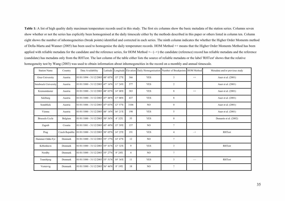
35
Table 1: A list of high quality daily maximum temperature records used in this study. The first six columns show the basic metadata of the station series. Columns seven
show whether or not the series has explicitly been homogenised at the daily timescale either by the methods described in this paper or others listed in column ten. Column
eight shows the number of inhomogeneities (break points) identified and corrected in each series. The ninth column indicates the whether the Higher Order Moments method
of Della-Marta and Wanner (2005) has been used to homogenise the daily temperature records. HOM Method ++ means that the Higher Order Moments Method has been
applied with reliable metadata for the candidate and the reference series, for HOM Method +− (−+) the candidate (reference) record has reliable metadata and the reference
(candidate) has metadata only from the RHTest. The last column of the table either lists the source of reliable metadata or the label 'RHTest' shows that the relative
homogeneity test by Wang (2003) was used to obtain information about inhomogeneities in the record on a monthly and annual timescale.
Station Name Country Data Availability Latitude Longitude Elevation Daily Homogenisation Number of Breakpoints HOM Method Metadata and/or previous study
Graz-University Austria 01/01/1894 - 31/12/2003 48° 05'N 15° 27'E 366 YES 3 ++ Auer et al. (2001)
Innsbruck-University Austria 01/01/1880 - 31/12/2003 47° 16'N 11° 24'E 577 YES 2 Auer et al. (2001)
Kremsmünster Austria 01/01/1880 - 31/12/2003 48° 03'N 14° 08'E 383 YES 8 ++ Auer et al. (2001)
Salzburg Austria 01/01/1880 - 31/12/2003 47° 48'N 13° 00'E 437 YES 8 Auer et al. (2001)
Sonnblick Austria 01/01/1886 - 31/12/2003 47° 03'N 12° 57'E 3106 NO 0 Auer et al. (2001)
Vienna Austria 01/01/1880 - 31/12/2003 48° 14'N 16° 21'E 198 YES 5 Auer et al. (2001)
Brussels-Uccle Belgium 01/01/1880 - 31/12/2003 50° 54'N 4° 32'E 55 YES 0 Demarée et al. (2002)
Zagreb Croatia 01/01/1881 - 31/12/2003 45° 49'N 15° 59'E 157 NO ? Prag Czech Republic 01/01/1880 - 31/12/2003 50° 05'N 14° 25'E 191 YES 4 −+ RHTest
Hammer-Odde-Fyr Denmark 01/01/1880 - 31/12/2003 55° 17'N 14° 47'E 12 NO ? Köbenhavn Denmark 01/01/1880 - 31/12/2003 55° 41'N 12° 32'E 9 YES 3 RHTest
Nordby Denmark 01/01/1880 - 31/12/2003 55° 27'N 8° 24'E 4 NO ? Tranebjerg Denmark 01/01/1880 - 31/12/2003 55° 51'N 10° 36'E 11 YES 3 −− RHTest
Vestervig Denmark 01/01/1880 - 31/12/2003 56° 46'N 8° 19'E 18 NO ?

36
Helsinki Finland 01/01/1880 - 31/12/2003 60° 19'N 24° 58'E 51 NO ? Paris-Parcmontsouris France 01/01/1880 - 31/12/2003 48° 49'N 2° 20'E 75 YES 5 ++ Caussinus and Mestre (2004)
Bamberg Germany 01/01/1880 - 31/12/2003 49° 53'N 10° 53'E 282 YES 3 ++ Herzog and Müller-Westermeier (1998)
Bremen Germany 01/01/1890 - 31/12/2003 53° 02'N 8° 47'E 5 YES 3 ++ Herzog and Müller-Westermeier (1998)
Frankfurt Germany 01/01/1880 - 31/12/2003 50° 07'N 8° 40'E 103 YES 1 ++ Herzog and Müller-Westermeier (1998)
Halle Germany 01/01/1900 - 31/12/2003 51° 29'N 11° 59'E 104 YES 1 ++ Herzog and Müller-Westermeier (1998)
Hamburg-Bergedorf Germany 01/01/1891 - 31/12/2003 53° 29'N 10° 15'E 35 YES 1 ++ Herzog and Müller-Westermeier (1998)
München Germany 01/01/1880 - 31/12/2003 48° 10'N 11° 30'E 515 YES 2 −+ Herzog and Müller-Westermeier (1998)
Münster Germany 01/01/1891 - 31/12/2003 51° 58'N 7° 36'E 63 YES 5 ++ Herzog and Müller-Westermeier (1998)
Potsdam Germany 01/01/1893 - 31/12/2003 52° 23'N 13° 04'E 81 NO 0 Herzog and Müller-Westermeier (1998)
Schwerin Germany 01/01/1890 - 31/12/2003 53° 38'N 11° 23'E 59 YES 2 ++ Herzog and Müller-Westermeier (1998)
Stuttgart Germany 01/01/1900 - 31/12/2003 48° 43'N 9° 13'E 401 YES 3 −+ Herzog and Müller-Westermeier (1998)
Dublin Ireland 01/01/1881 - 31/12/2003 53° 22'N 6° 21'W 68 NO ? De-Bilt Netherlands 01/01/1901 - 31/12/2003 52° 06'N 5° 11'E 2 YES 3 ++ Pers. comms Albert Klein Tank
Eelde Netherlands 01/03/1906 - 31/12/2003 53° 08'N 6° 35'E 4 YES 3 ++ Pers. comms Albert Klein Tank
Lisboa-Geofisica Portugal 01/01/1901 - 31/12/2003 38° 43'N 9° 09'W 77 YES 4 −+ Albacete Spain 14/11/1893 - 31/12/2003 38° 57'N 1° 52'W 704 YES 1 Brunet et al. (2006b)
Badajoz Spain 01/01/1880 - 31/12/2003 38° 53'N 6° 50'W 185 YES 2 Brunet et al. (2006b)
Burgos Spain 01/12/1880 - 31/12/2003 42° 22'N 3° 43'W 881 YES 2 Brunet et al. (2006b)
Ciudad Real Spain 01/12/1893 - 31/12/2003 38° 59'N 3° 55'W 627 YES 6 Brunet et al. (2006b)
Granada Spain 01/11/1893 - 31/12/2003 37° 08'N 3° 38'W 680 YES 2 Brunet et al. (2006b)
Madrid Spain 01/01/1880 - 31/12/2003 40° 25'N 3° 41'E 667 YES 2
Brunet et al. (2006b)

37
Pamplona Spain 01/04/1880 - 31/12/2003 42° 46'N 1° 38'W 459 YES 3 Brunet et al. (2006b)
Salamanca Spain 01/11/1893 - 31/12/2003 40° 57'N 5° 29'W 618 YES 3 Brunet et al. (2006b)
Soria Spain 18/11/1893 - 31/12/2003 41° 26'N 2° 29'E 1082 YES 1 Brunet et al. (2006b)
Valladolid Spain 12/12/1893 - 31/12/2003 41° 38'N 4° 46'W 735 YES 2 Brunet et al. (2006b)
Zaragoza Spain 01/09/1887 - 31/12/2003 41° 40'N 1° 01'W 247 YES 2 Brunet et al. (2006b)
Falun Sweden 01/10/1902 - 31/12/2003 60° 37'N 15° 40'E 157 YES 2 −+ RHTest
Stensele Sweden 01/01/1891 - 31/12/2003 65° 04'N 17° 09'E 325 NO ? Stockholm Sweden 01/01/1880 - 31/12/2003 59° 21'N 18° 03'E 44 YES 1 ++ Moberg et al. (2002)
Uppsala Sweden 01/01/1880 - 31/12/2003 59° 52'N 17° 38'E 13 YES 3 ++ Bergström and Moberg (2002)
Växjö Sweden 01/01/1891 - 31/12/2003 56° 52'N 14° 48'E 166 NO ? Basel Switzerland 01/01/1901 - 31/12/2003 47° 33'N 7° 35'E 316 YES 6 ++ Begert et al. (2005)
Bern Switzerland 01/01/1880 - 31/12/2003 46° 56'N 7° 25'E 570 YES 8 ++ Begert et al. (2005)
Geneva Switzerland 01/01/1880 - 31/12/2003 46° 15'N 6° 08'E 420 YES 2 ++ Begert et al. (2005)
Lugano Switzerland 01/07/1880 - 31/12/2003 46° 00'N 8° 58'E 273 YES 4 Begert et al. (2005)
Säntis Switzerland 01/01/1901 - 31/12/2003 47° 15'N 9° 21'E 2490 YES 5 Begert et al. (2005)
Zürich Switzerland 01/01/1882 - 31/12/2003 47° 23'N 8° 34'E 556 YES 6 ++ Begert et al. (2005)
Armagh United Kingdom 01/01/1880 - 31/12/2003 54° 21'N 6° 65'W 62 YES 3 ++ Butler et al. (2005)
CET United Kingdom 01/01/1880 - 31/01/2003 52° 25'N 1° 50'W 78 YES 3 Parker and Horton (2005); Parker et al. (1992)

38
Table 2: Summary of predictor and predictand variables, their resolution and their domain. All SLP data came
from the dataset described in Ansell et al. (2005) and section 2.1, SST data are described in Smith and Reynolds
(2004) and section 2.1 and the majority of the precipitation data are from Mitchell and Jones (2005) updated
with data from Huffman et al. (1997) (see section 2.1 for more detail). The last column shows the number of
significant principle components retained (Npc) and their total explained variance (see section 2.3 for more
information on the method). ‡The HWPC1 index is the first principle component of JJA HW index that has been
smoothed using a LOESS function with a smoothing parameter of 25 years (Cleveland and Devlin (1988)), de-
trended and standardised to have a variance of one and a mean of zero. †The AMO index was calculated using
annually averaged SST in the domain specified in the table (according to the definition in Sutton and Hodson
(2005)) and then smoothed using a LOESS function with a smoothing parameter of 25 years. This was then de-
trended and standardised to have a variance one and mean of zero.
Element Predictor Season Resolution Domain Npc,
Abbreviation /month (% Exp. var)
Predictand
Heat Wave index HW JJA - See figure 1 4 (69) Heat Wave Principle Component 1‡ HWPC1 JJA - See figure 1 1 (37) Hot Days index HD JJA - See figure 1 4 (68) Mean Maximum Temperature TXAV JJA - See figure 1 4 (68)
Predictor
North Atlantic Sea Level Pressure SLP JJA 5°× 5° 70°W - 50°E, 25°N - 70°N 12 (86)
North Atlantic Sea Surface Temperature SSTNA JJA 2.5°× 2.5° 70°W - 50°E, 25°N - 70°N 14 (91)
North Atlantic Sea Surface Temperature SSTNA MAM 2.5°× 2.5° 70°W - 50°E, 25°N - 70°N 13 (87)
North Atlantic Sea Surface Temperature SSTNA DJF 2.5°× 2.5° 70°W - 50°E, 25°N - 70°N 14 (89)
North Atlantic Sea Surface Temperature SSTAT DJF 2.5°× 2.5° 70°W - 50°E, 0°N - 70°N 15 (88)
Atlantic Multidecadal Oscillation† AMO Annual 2.5°× 2.5° 75°W - 7.5°W, 0°N - 60°N -
Western Europe Precipitation PRECWE JJA 0.5°× 0.5° 15°W - 20°E, 35°N - 60°N 14 (71)
Mediterranean Precipitation PRECME JFMAM 0.5°× 0.5° 70°W - 50°E, 42°N - 46°N 8 (81)
Northern South America Precipitation PRECNSA June 0.5°× 0.5° 85°W - 49.5°W, 0°N - 15°N 15 (82)
Brazilian Precipitation PRECBR June 0.5°× 0.5° 65°W - 29.5°W, 2.5°S - 15°S 13 (86)
Sahel Precipitation PRECSH June 0.5°× 0.5° 20°W - 64.5°E, 10°N - 20°N 17 (77)
Sahel Precipitation PRECSH July 0.5°× 0.5° 20°W - 64.5°E, 10°N - 20°N 16 (76)
Sahel Precipitation PRECSH August 0.5°× 0.5° 20°W - 64.5°E, 10°N - 20°N 13 (77)

39
Table 3: Summary of the CCAs between various predictors (see table 2 for details) and JJA HW. The first three
columns show the predictor(s) abbreviation, the season the predictor was averaged over and the number of PCs
retained to build the CCA (NCCA) after cross-validation respectively. The column titled CCA shows the number
predictand PCs retained after cross-validation, r is the canonical correlation between the score series, % var.
exp. is the percentage of explained variance of JJA HWs for each CCA, µhindcast is the average hindcast
Spearman rank correlation skill score of all stations with an approximate 95% confidence interval to show the
spread of results using the 1880-1965 period to build the model and 1966-2003 to validate the model (in the case
where a precipitation predictor was used the period 1901-1971 was used to build the model and remaining
period used to validate the model). The last column gives a brief description of the hindcast skill. See section 2.3
for details on the CCA model selection method.
Predictor(s) Season NCCA CCA r % var.
exp. µhindcast Model skill description
SLP JJA 12 1 0.81 16.6 0.47±0.42 Good skill over 2 0.72 8.4 the entire domain,
3 0.63 2.5 except the Alps.
4 0.46 4.4
TOTAL - 32.0
SSTNA JJA 14 1 0.76 20.2 0.54±0.25 Good skill over 2 0.73 5.9 the entire domain.
3 0.64 6.5
4 0.48 1.7
TOTAL - 34.3
SSTNA DJF 6 1 0.38 1.6 0.12±0.35 Generally poor skill over
2 0.29 1.6 the entire domain.
3 0.20 0.5 Iberian Peninsula
4 0.19 1.2 skill score around 0.5
TOTAL - 4.9
SSTNA MAM 2 1 0.33 3.9 0.21±0.38 Generally poor skill over
2 0.03 0.0 the entire domain. Highest
TOTAL - 3.9 values over central western Europe (0.5)
PRECWE JJA 5 1 0.76 13.4 0.49±0.30 Good skill over 2 0.71 11.5 the entire domain
3 0.54 2.7
4 0.37 2.2
TOTAL - 29.8
PRECME JFMAM 2 1 0.42 6.2 0.23±0.48 Generally poor skill over
2 0.03 0.0 the entire domain. However central
TOTAL - 6.2 Europe between 0.3 - 0.5 (see figure 8d)
PRECBR Jun 4 1 0.46 4.4 0.23±0.36 Generally moderate skill over
PRECNSA Jun
2 0.28 1.6 the entire domain, 0.3-0.5.

40
PRECSH Aug 3 0.18 0.2 Poor skill over the Alpine region
4 0.02 0.0
TOTAL - 6.2
PRECBR Jun 31 1 0.86 16.5 0.27±0.37 Moderate skill most PRECNSA Jun 2 0.78 8.2 of the domain 0.3-0.6. PRECSH Aug 3 0.69 7.8 However, poor over the Alpine region
SLP JJA 4 0.51 5.1
TOTAL - 37.6
PRECSH Jun 37 1 0.87 15.8 0.35±0.32 Moderate to good skill over
PRECSH Jul 2 0.85 23.9 most of the domain 0.3-0.6.
PRECSH Aug 3 0.75 3.3 However, poor over the Alpine region
SLP JJA 4 0.63 4.9 and parts of the Iberian Peninsula
TOTAL - 47.9
SLP JJA 12 1 0.86 14.2 0.60±0.29 Good skill over SSTNA JJA 2 0.83 19.6 the domain, up to 0.84
PRECWE JJA 3 0.72 6.7
4 0.64 4.5
TOTAL - 45.0
SSTAT DJF 8 1 0.56 10.1 0.28±0.28 Generally moderate to poor
PRECME JFMAM 2 0.43 1.4 skill over the domain.
3 0.22 0.3 Skill up to 0.55 in
4 0.16 0.6 central western Europe
TOTAL - 12.4 (see figure 13e)

41
Figure 1: The long-term linear trend of the HW index in units of frequency per decade calculated over the
longest possible period for each station (see table 1 for the details). The size of the crosses ('+') and the open
circle ('o') denote the magnitude of the positive and negative trends according to the legend on the left side of
the figure respectively.
Figure 2: The long-term linear trend in JJA averaged SLP in hPa per decade calculated over the 1880 to 2003
period. Stippled areas show statistically significant trends at the 90% confidence level.
Figure 3: The long-term linear trend in JJA averaged SSTNA in °C per decade calculated over the 1880 to 2003
period. Stippled areas show statistically significant trends at the 90% confidence level.

42
Figure 4: The long-term linear trend in JJA averaged PRECWE in mm per decade calculated over the 1901 to
2003 period. Stippled areas show statistically significant trends at the 90% confidence level.
a) b)
c)
Figure 5: The first CCA between JJA averaged SLP and the JJA HW index which explains approximately
16.6% of JJA HW variability. The SLP canonical pattern a), b) the HW canonical pattern and c) the canonical
score series from 1880 to 2003. In b) the size of the crosses ('+') and open circles ('o') show the canonical
loadings expressed as a correlation coefficient for each station according to the legend on the left of the figure.
In c) the solid and dashed lines are the SLP and HW canonical score series respectively with a correlation
coefficient of 0.81.

43
a) b)
c)
Figure 6: The second CCA between JJA averaged SLP and the JJA HW index which explains approximately
8.4% of JJA HW variability. The SLP canonical pattern a), b) the HW canonical pattern and c) the canonical
score series from 1880 to 2003. In b) the size of the crosses ('+') and open circles ('o') show the canonical
loadings expressed as a correlation coefficient for each station according to the legend on the left of the figure.
In c) the solid and dashed lines are the SLP and HW canonical score series respectively with a correlation
coefficient of 0.72.
a) b)
Figure 7: A timeseries plot a), showing the smoothed Atlantic Multidecadal Oscillation (AMO, dashed line)
index and the smoothed first principle component of JJA HWs (HWPC1) from 1880 to 2003 and b) the loading
patterns associated with the raw (unsmoothed) first principle component (PC). In b), the size of the crosses ('+')
and the open circles ('o') denote the magnitude of the positive and negative PCA loadings according to the
legend on the left side of the figure. The correlation between the two timeseries is 0.8, however it is hard to
determine the statistical significance due to the limited number of degrees of freedom. The first PC of the HW
index explains 37% of HW variability. The two timeseries have been smoothed using a LOESS smoother with a
period set approximately to 25 years. See table 2 for more details on each index.

44
a) b)
c)
d)
Figure 8: The first CCA between JFMAM averaged PRECME and the JJA HW index which explains
approximately 6.2% of JJA HW variability. The canonical PRECME pattern a), b) the HW canonical pattern
and c) the canonical score series from 1901 to 2003. In b) the size of the crosses ('+') and open circles ('o') show
the canonical loadings expressed as a correlation coefficient for each station according to the legend on the left
of the figure. In c) the solid and dashed lines are the PRECME and HW canonical score series respectively with
a canonical correlation of 0.42. The Spearman rank hindcast skill score d) of the CCA between JFMAM
averaged PRECME and the JJA HW index. The model was built in the period 1901-1971 and the model
hindcast in the remaining, 1972-2003 period. The size of the crosses ('+') and open circles ('o') shows the
magnitude of the skill score according to the legend on the left of the figure.

45
a) b)
c) d)
e)
f)
Figure 9: The first multiple predictor CCA between June, July, August PRECSH, JJA averaged SLP and the
JJA HW index which explains approximately 15.8% of JJA HW variability. The June a), July b) and August c)
PRECSH canonical pattern, d) the JJA SLP canonical pattern, e) the HW canonical pattern and f) the canonical
score series from 1901 to 2003. In e) the size of the crosses ('+') and open circles ('o') show the canonical
loadings expressed as a correlation coefficient for each station according to the legend in the left of the figure. In
f) the solid and dashed lines are the multiple predictor and HW canonical score series respectively with a
canonical correlation of 0.87.

46
a) b)
c) d)
e)
f)
Figure 10: The second multiple predictor CCA between June, July, August PRECSH, JJA averaged SLP and
the JJA HW index which explains approximately 23.5% of JJA HW variability. The June a), July b) and August
c) PRECSH canonical pattern, d) the JJA SLP canonical pattern, e) the HW canonical pattern and f) the
canonical score series from 1901 to 2003. In e) the size of the crosses ('+') and open circles ('o') show the
canonical loadings expressed as a correlation coefficient for each station according to the legend in the left of
the figure. In f) the solid and dashed lines are the multiple predictor and HW canonical score series respectively
with a canonical correlation of 0.85.

47
a) b)
c) d)
e)
Figure 11: The first multiple predictor CCA between JJA averaged SLP, SSTNA, PRECWE and the JJA HW
index which explains approximately 14.2% of JJA HW variability. The SLP canonical pattern a), b) the SSTNA
canonical pattern, c) the PRECWE canonical pattern, d) the HW canonical pattern and e) the canonical score
series from 1901 to 2003. In d) the size of the crosses ('+') and open circles ('o') show the canonical loadings
expressed as a correlation coefficient for each station according to the legend in the left of the figure. In e) the
solid and dashed lines are the multiple predictor and HW canonical score series respectively with a canonical
correlation of 0.86.

48
a) b)
c) d)
e)
Figure 12: The second multiple predictor CCA between JJA averaged SLP, SSTNA, PRECWE and the JJA
HW index which explains approximately 19.6% of JJA HW variability. The SLP canonical pattern a), b) the
SSTNA canonical pattern, c) the PRECWE canonical pattern, d) the HW canonical pattern and e) the canonical
score series from 1901 to 2003. In d) the size of the crosses ('+') and open circles ('o') show the canonical
loadings expressed as a correlation coefficient for each station according to the legend in the left of the figure. In
e) the solid and dashed lines are the multiple predictor and HW canonical score series respectively with a
canonical correlation of 0.83.

49
a) b)
c)
d)
e)
Figure 13: The first multiple predictor CCA between DJF averaged SSTAT, JFMAM PRECME and the JJA
HW index which explains approximately 10.1% of JJA HW variability. The SSTNA canonical pattern a), b) the
PRECWE canonical pattern, c) the HW canonical pattern and d) the canonical score series and e) the hindcast
(1982-2003) Spearman rank correlation skill score. In c) and e) the size of the crosses ('+') and open circles ('o')
show the canonical loadings expressed as a correlation coefficient and the Spearman rank correlation skill score
respectively for each station. In d) the solid and dashed lines are the multiple predictor and HW canonical score
series respectively with a canonical correlation of 0.56.