Linear Filtering• Linear case is simplest and most useful

– Replace each pixel with a linear combination of its neighbors.

• The prescription for the linear combination is called the convolution kernel.

10 5 34 5 11 1 7

70 0 0

0 0.5 00 1.0 0.5

=*kernel

Frequency-Domain Filtering• Compute the Fourier Transform of the image• Multiply the result by filter transfer function• Take the inverse transform

Frequency-Domain Filtering

Frequency-Domain Filtering• Ideal Lowpass Filters

>> [f1,f2] = freqspace(256,'meshgrid');>> H = zeros(256,256); d = sqrt(f1.^2 + f2.^2) < 0.5;>> H(d) = 1;>> figure; imshow(H);

Non-separable

2 201, for ( , )

0, otherwiseu v DH u v

⎧⎪ + ≤= ⎨⎪⎩

Separable

1, for and ( , )

0, otherwiseu vu D v D

H u v≤ ≤⎧

= ⎨⎩

>> [f1,f2] = freqspace(256,'meshgrid');>> H = zeros(256,256); d = abs(f1)<0.5 & abs(f2)<0.5;>> H(d) = 1;>> figure; imshow(H);

Frequency-Domain Filtering• Butterworth Lowpass Filter

22 2

0

1( , )1

nH u vu v D

=⎡ ⎤+ +⎣ ⎦ As order increases the

frequency response approaches ideal LPF

Frequency-Domain Filtering• Butterworth Lowpass Filter

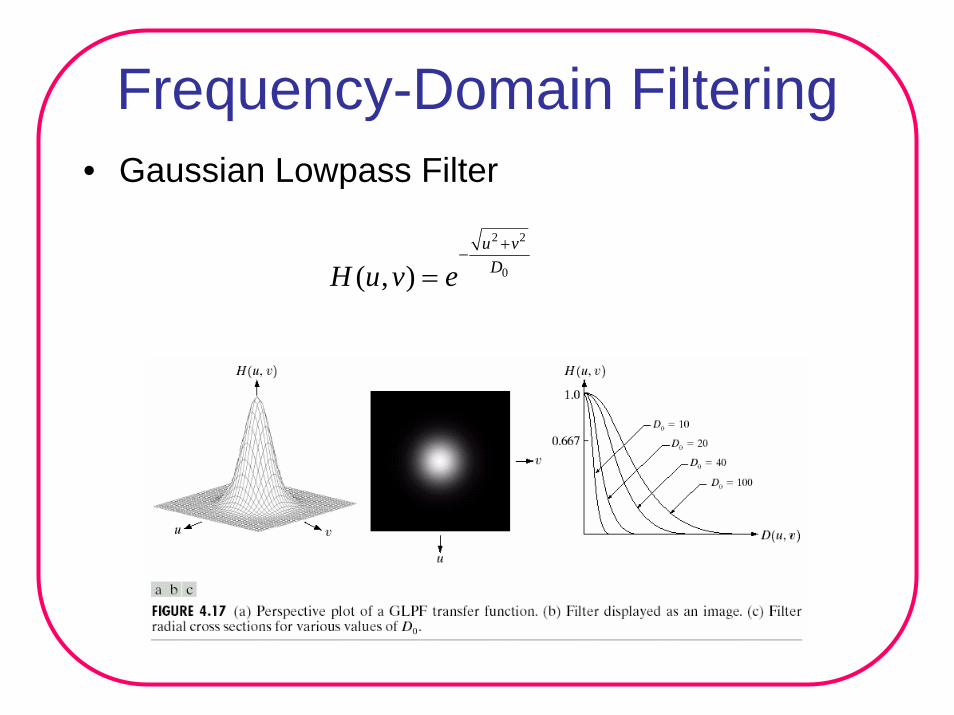
Frequency-Domain Filtering• Gaussian Lowpass Filter

2 2

0( , )u vDH u v e

+−

=

Frequency-Domain FilteringIdeal LPF Butterworth LPF Gaussian LPF

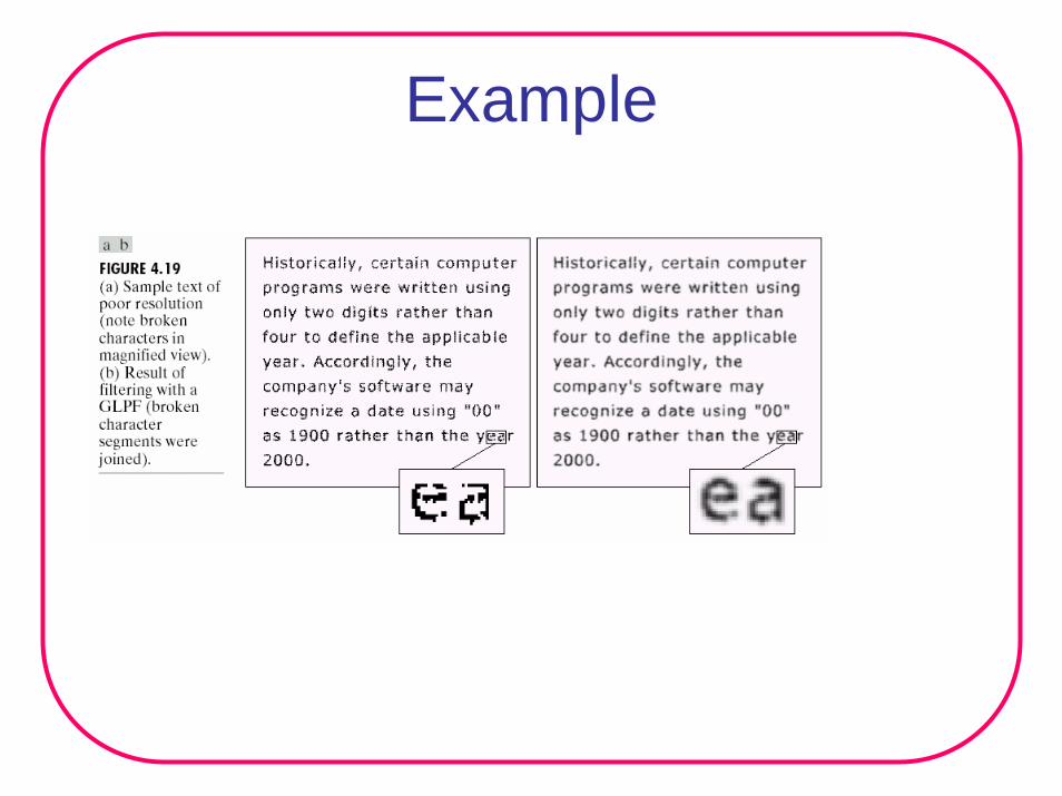
Example

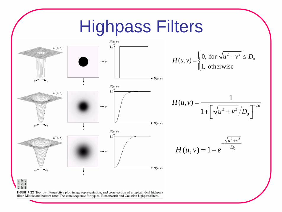
Highpass Filters2 2

00, for ( , )1, otherwise

u v DH u v⎧⎪ + ≤= ⎨⎪⎩

22 2

0

1( , )1

nH u vu v D

−=⎡ ⎤+ +⎣ ⎦

2 2

0( , ) 1u vDH u v e

+−

= −

Notch filter

• It is a kind of bandreject/bandpass filter that rejects/passes a very narrow set of frequencies, around a center frequency.

• Due to symmetry considerations, the notches must occur in symmetric pairs about the origin of the frequency plane.

• The transfer function of an ideal notch-reject filter of radius D0 with center frequency (u0, v0) is given by

⎩⎨⎧

=10

),( vuHD1(u0, v0) ≤ D0 Or D2(u0, v0) ≤ D0

otherwise

where [ ] 2/120

201 )2/()2/(),( vNvuMuvuD −−+−−=

[ ] 2/120

202 )2/()2/(),( vNvuMuvuD +−++−=

• The transfer function of a Butterworth notch reject filter of order n is given by

n

vuDvuDD

vuH

⎥⎦

⎤⎢⎣

⎡+

=

),(),(1

1),(

21

20

• A Gaussian notch reject filter is given by

)),(),(21exp(1),( 2

0

21⎥⎦

⎤⎢⎣

⎡−−=

DvuDvuDvuH

• A notch pass filter can be obtained from a notch reject filter using:

Hnp(u, v) =1 – Hnr (u, v)

Illustration of transfer function of notch filters

Example

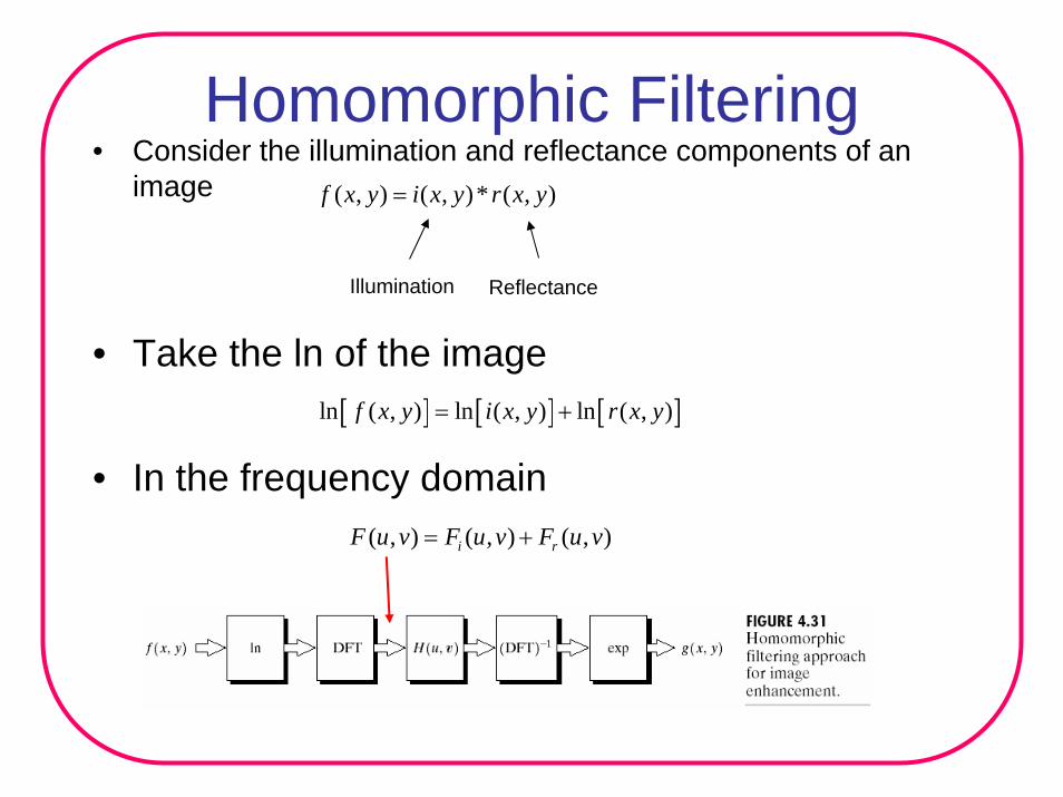
Homomorphic Filtering• Consider the illumination and reflectance components of an

image ( , ) ( , )* ( , )f x y i x y r x y=

Illumination Reflectance

• Take the ln of the image[ ] [ ] [ ]ln ( , ) ln ( , ) ln ( , )f x y i x y r x y= +

• In the frequency domain( , ) ( , ) ( , )i rF u v F u v F u v= +

Homomorphic Filtering• The illumination component of an image shows

slow spatial variations. • The reflectance component varies abruptly. • Therefore, we can treat these components

somewhat separately in the frequency domain.

1

With this filter, low-frequency components are attenuated, high-frequency components are emphasized.

Homomorphic Filtering

0.52.0

L

H

γγ

==

Adaptive local noise reduction filter

• Filter operation is not uniform at all pixel locations but depends on the local characteristics (local mean, local variance) of theobserved image.• Consider an observed image g(m,n) and an a X b window Sab . Let σ2 be the noise variance , mL(m, n), σL

2 (m, n) σ be the local mean and variance of g(m,n) over an a X b window around (m,n). • The adaptive filter is given by:

)),(),((),(

),(),(ˆ2

2

nmmnmgnm

nmgnmf LL

−−=σ

σ η

• Usually, we need to be careful about the possibility of),(22 nmLσσ η > , in which case, we could potentially get a

negative output gray value.

• This filter does the following:

(1) If (or is small), the filter simply returns the value of g(m,n).

02 =ησ

(2) If the local variance is high relative to the noise variance the filter returns a value close to g(m,n). This usually corresponds to a location associated with edges in the image.

),(2 nmLσ

(3)If the two variances are roughly equal, the filter does a simple averaging over window Sab .

• Only the variance of overall noise has to be estimated.

Linear, position-invariant degradation

• The general degradation equation:

g(m,n) = h(m,n)*f(m,n) + η(m,n)

G(u,v) = H(u,v)F(u,v) + N(u,v)

• This consists of a “blurring” function h(m,n), in addition the random noise component η(m,n).

• The blurring function h(m,n) is usually referred to as a point-spread function (PSF) and represents the observed image corresponding to imaging an impulse or point source of light.

• In this case, we need to have a good knowledge of the PSF h(m,n), in addition to knowledge of the noise statistics. This can be done in practice using one of the following methods:

Using Image observation

• Identify portions of the observed image (subimage) that are relatively noise-free and which corresponds to some simple structures.

• We can then obtain),(ˆ),(

),(vuFvuG

vuHs

ss =

where Gs(u,v) is the spectrum of the observed subimage,

is our estimate of the spectrum of the original image (based on the simple structure that the subimage represents).

),(ˆ vuFs

• Based on the characteristic of the function Hs(u,v), we can rescale to obtain the overall PSF H(u ,v).

Inverse Filter

• In the DFT domain, the inverse filter H-1 is defined byH-1 (u,v) = 1/H(u,v)

• The simplest approach to restoration is direct inverse filtering. This is obtained as follows:

),(),(),(ˆ

vuHvuGvuF =

• Note there is a problem of division by zero

Because of G(u,v) = H(u,v)F(u,v) + N(u,v)

),(),(),(),(ˆ

vuHvuNvuFvuF += Where H(u,v): degradation function

• Hence noise actually gets amplified at frequencies where H(u,v) is zero or very small. In fact, the contribution from the noise term dominates at these frequencies.

• It is therefore, seldom used in practice, in the presence of noise.

• Note that the inverse filter of a low-pass distortion is always a high-pass variety

Wiener Filter

• Also known as “Minimum Mean Square Error Filter”

• Norbert Wiener introduced this filter

• The DFT of the Wiener filter is given by:

2

*( , )( , )| ( , ) |Wiener

H u vH u vH u v K

=+

where K is a constant (designer has to experiment various of K)• Assumptions:

(1)Image and noise as random process

(2) Image and noise are uncorrelated

(3) Noise is a spectrally white noise and has zero mean (in spatial domain)

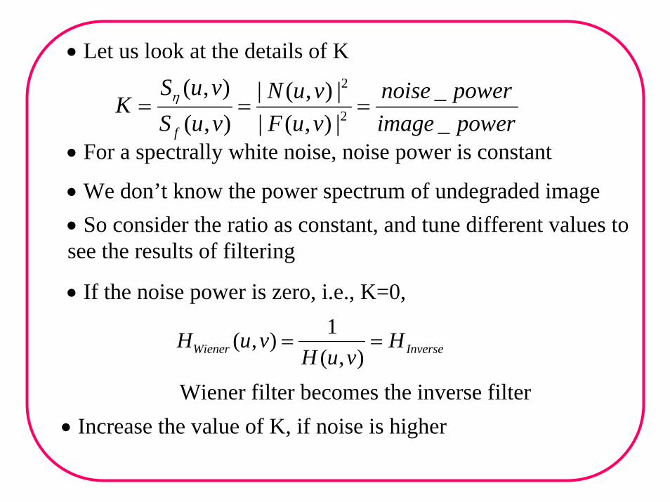
• Let us look at the details of K2

2

( , ) | ( , ) | _( , ) | ( , ) | _f

S u v N u v noise powerKS u v F u v image power

η= = =

• For a spectrally white noise, noise power is constant

• We don’t know the power spectrum of undegraded image• So consider the ratio as constant, and tune different values tosee the results of filtering

• If the noise power is zero, i.e., K=0, 1( , )

( , )Wiener InverseH u v HH u v

= =

Wiener filter becomes the inverse filter• Increase the value of K, if noise is higher

More Noise (Gaussian)

Less Noise

Degraded Image Inverse Filter Wiener Filter

Comments

• Wiener filter is the MMSE linear filter.

• Wiener filter may be optimal, but it isn’t always good.

• Linear filters blur edges

• Linear filters work poorly with non-Gaussian noise.

• Nonlinear filters can be designed using the same method-ologies.

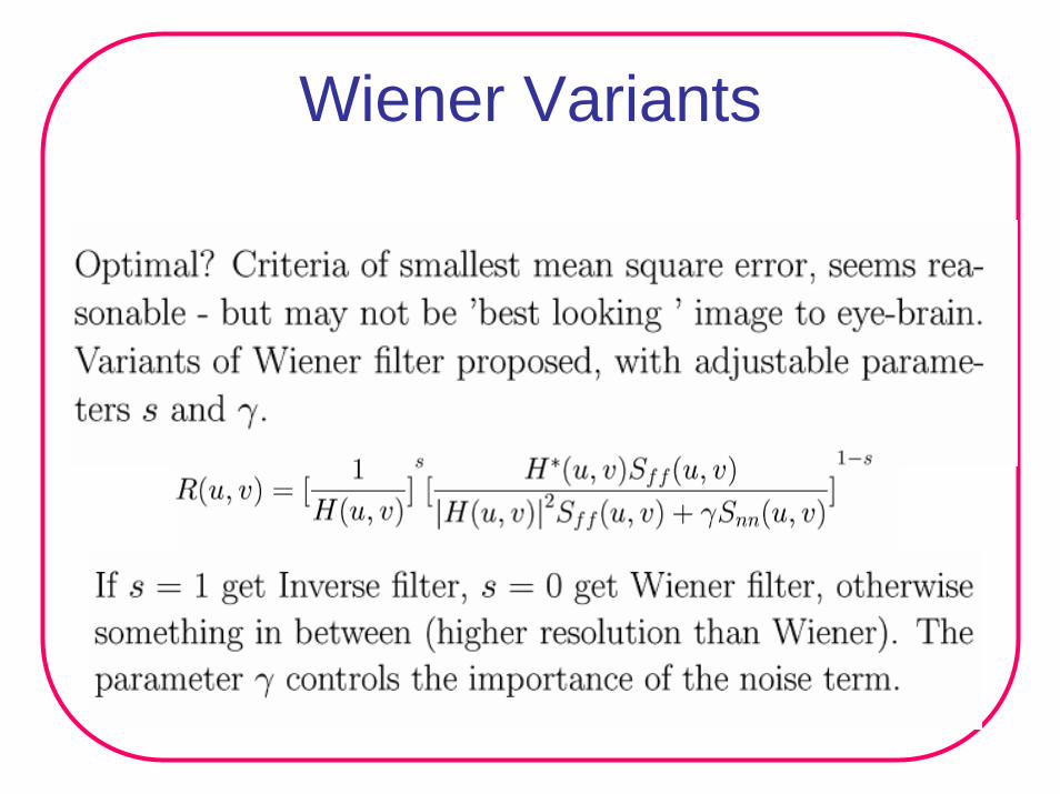
Wiener Variants

Constrained Optimization (noise power)

• Tune using two parameters

Local Statistics and Locally Optimal Filters

• Adaptive local statistics filters (Section 16) comprised of local masks or local difference equations whose coefficients were functions of the local signal and noise characteristics.

• In both cases, we assumed a simple structure and then found optimal values for the parameters in some fashion.

Signal model

• An alternative strategy is to adopt a local signal model and let the locally optimal filter structure conform to the output to the model.

• That is, we find a locally optimal, minimum mean squared error estimator that adapts to signal non-stationarity.

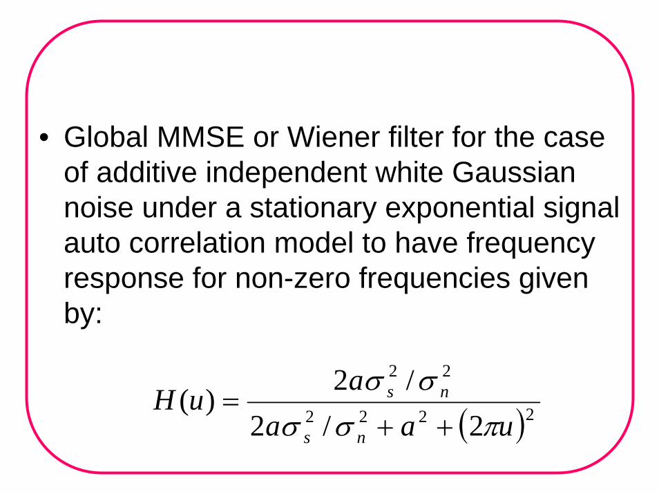
• Global MMSE or Wiener filter for the case of additive independent white Gaussian noise under a stationary exponential signal auto correlation model to have frequency response for non-zero frequencies given by:

( )2222

22

2/2/2

)(uaa

auH

ns

ns

πσσσσ

++=

• This is an exponential low pass filter with impulse response:

•x

ea

xhsn

β

σσβ −

+= 22 2/1

2/)(

with bandwidth

where .πβ 2/

222 /2 nsaa σσβ +=

• A simple strategy for a locally optimal filter is to allow the signal statistics to vary.

• That is the filter behaves as a function of signal variance

• Noise variance is assumed to be constant, and we will take the auto correlation parameter a to be constant as well for simplicity.

• At edges and texture regions of strong local contrast, the signal variance will increase causing the bandwidth to increase and the spatial extent of the smoothing effect to decrease.

• Thus: Less smoothing is done at edges and textured regions and more is done in regions of constant smoothing, addressing the primary deficiency of the global Wiener filter.

Implementation

• Sample and truncate the impulse response or find a local difference equation whose impulse response is a sampled version of

• Derive the filter by starting with a discrete signal model.

)(xh

Adapting the AC of the signal

• Consider a discrete signal model with exponential auto-correlation function:

)()()( 22 nn

annR sss µσ +=

• Note that the signal mean and variance to be spatially dependent, while the correlation parameter is assumed to be constant:

( ) 22 /)1( sssRa σµ−=

The corresponding local power spectrum is:

( ) ( ))()(

2cos211)( 2

2

222 un

uaaan

eP ssuj

s δµπ

σπ +−+

−=

• Assuming stationary Gaussian white noise model with power spectrum

• the local minimum mean squared error estimator, or Wiener filter is

• with a DC gain of one for zero mean noise.

( ) 22n

ujn eP σπ =

( ) ( )( ) 0 ,

2cos2/)(11/)(12222

2222 ≠

−−++−

= uuanaa

naeHns

nsuj

πσσσσπ

• The corresponding local system transfer function is:

( ) ( )( ) 12222

222

/)(11/)(1

−−−−++−

=azaznaa

nazH

ns

ns

σσσσ

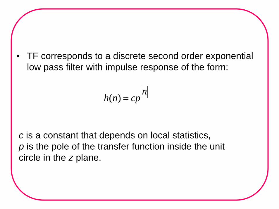
• TF corresponds to a discrete second order exponential low pass filter with impulse response of the form:

ncpnh =)(

c is a constant that depends on local statistics, p is the pole of the transfer function inside the unit circle in the z plane.

• This non-causal filter has a second pole at 1/p, where

242 −−

=ββ

p

For

2

2 )(11

n

s na

aaa

σσ

β ⎟⎠⎞

⎜⎝⎛ −++=

2

2 )(11

n

s naaa

aσ

σβ ⎟⎠⎞

⎜⎝⎛ −++=

242 −−

=ββ

p

• As the signal to noise variance ratio increases, the poles move toward 0 and and the filter becomes an all pass filter.

• As the SNR goes to 0, the poles approach • and• the filter does maximal smoothing consistent

with the local correlation coefficient.

∞

a/1a

• The local difference equation for this optimal adaptive filter is:

)1()1()()(1)(

)(112

2

2

2

++−+⎟⎠⎞

⎜⎝⎛ −=⎟⎟

⎠

⎞⎜⎜⎝

⎛⎟⎠⎞

⎜⎝⎛ −++ ngngnf

na

ang

na

aa

a n

s

n

s

σσ

σσ

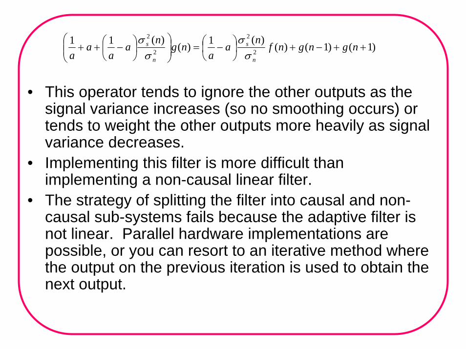
)1()1()()(1)(

)(112

2

2

2

++−+⎟⎠⎞

⎜⎝⎛ −=⎟⎟

⎠

⎞⎜⎜⎝

⎛⎟⎠⎞

⎜⎝⎛ −++ ngngnf

na

ang

na

aa

a n

s

n

s

σσ

σσ

• This operator tends to ignore the other outputs as the signal variance increases (so no smoothing occurs) or tends to weight the other outputs more heavily as signal variance decreases.

• Implementing this filter is more difficult than implementing a non-causal linear filter.

• The strategy of splitting the filter into causal and non-causal sub-systems fails because the adaptive filter is not linear. Parallel hardware implementations are possible, or you can resort to an iterative method where the output on the previous iteration is used to obtain the next output.

• As long as the system is stable, the response will converge. Finally, you could explicitly find the impulse response as a function of local statistics and truncate it at some appropriate width to obtain a local statistics dependent mask. Figure 17.1 shows the effect of applying this locally optimal filter to an image corrupted with additive noise. For noise variance .01 with a normalized image (intensity scaled between 0 and 1), the iterative implementation converged in 16 iterations.

•

• Figure 17.1. Local Wiener filter, exponential signal model, iterative implementation.

With additive noise With local Wiener filter

• A similar locally optimal strategy has been suggested for the multiplicative noise case. The frequency response for a continuous Wiener filter for multiplicative noise is:

)()()(

)(uPuP

uPuH

ns

s

∗=

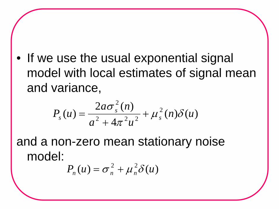
• If we use the usual exponential signal model with local estimates of signal mean and variance,

and a non-zero mean stationary noise model:

)()(4

)(2)( 2

222

2

unua

nauP s

ss δµ

πσ

++

=

)()( 22 uuP nnn δµσ +=

• (For multiplicative noise the mean is often taken to be one.) Evaluating the frequency response by performing the convolution of the signal and noise spectra leads to

• where

( )222

22

4/

)(u

auH n

πβµβ

+−

=

( ))()()(2222

2222

nnna

assn

sn

σµσσµ

β+

+=

• This is an exponential low pass filter with local impulse response

• Sampling and truncating this continuous impulse response yields a local statistics dependent mask for the adaptive filtering of multiplicative noise.

xeaxh

n

β

βµβ −−

= 2

22

)(

• The parameter• which determines the degree of

smoothing, depends on both local signal mean and variance.

• As the signal mean increases, decreases and more smoothing occurs. As the local signal to noise variance ratio increases, increases and less smoothing occurs.

β

β

β

• The filter does maximal smoothing in regions of high constant signal intensity, where multiplicative noise is most apparent.