summary report... · web viewthe pressures potentially responsible for causing most impacts in the...

The assessment of cumulative impacts using the Baltic Sea Pressure Index and the Baltic Sea Impact Index - supplementary report to the HELCOM ‘State of the Baltic Sea’ report

The production of this report has been carried out through the HELCOM Project for the development of the second holistic assessment of the Baltic Sea (HOLAS II). The methodology was developed through the HELCOM TAPAS project and the assessment was carried out by the HELCOM SPICE project. The work was financially supported through HELCOM and the EU co-financing of the HELCOM coordinated projects TAPAS and SPICE.

Contributors: Samuli Korpinen1, Marco Nurmi1, Henrik Nygård1, Leena Laamanen1,2, Joni Kaitaranta2, , Henna Rinne2, Kai Hoppe3, Emilie Kallenbach4, Ciaràn Murray5, Jesper Andersen4, Juuso Haapaniemi2 , Lena Bergström2

Acknowledgements: The spatial data underlying the assessment was based on national data calls supported by national experts and the HELCOM Contracting Parties, and by the achievements of HELCOM expert networks. The sensitivity scores were designed based on the contribution from experts in all nine contracting parties, and from the EU co-financed BalticBOOST project. The assessment method was developed by support of the EU co-financed TAPAS project, and by participants of the workshops HELCOM HOLAS II Pressure index WS 1-2015, HELCOM TAPAS Pressure index WS 1-2016, HELCOM TAPAS Pressure index WS 2-2016 , and HELCOM BSPI BSII 1-2018 . The assessment was carried out with support from the EU co-financed HELCOM SPICE project, and was guided by the HOLAS II Core team and HELCOM State & Conservation.

For bibliographic purposes, this document should be cited as:HELCOM (2018): The assessment of cumulative impacts using the Baltic Sea Pressure Index and the Baltic Sea Impact Index - supplementary report to the HELCOM ‘State of the Baltic Sea’ report. Available at: http://stateofthebalticsea.helcom.fi/about-helcom-and-the-assessment/downloads-and-data/Information included in this publication or extracts thereof are free for citing on the condition that the complete reference of the publication is given as above.Copyright 2018 by the Baltic Marine Environment Protection Commission – HELCOMCover photo: Cezary Korkosz

1 Finnish Environment Institute (SYKE)2 Baltic Marine Environment Protection Commission (HELCOM)3 IOW/BfN Germany4 NIVA Denmark5 NIVA Denmark

ASSESSMENT OF CUMULATIVE IMPACTS – FIRST VERSION 2017

http://stateofthebalticsea.helcom.fi/about-helcom-and-the-assessment/downloads-and-data/

https://portal.helcom.fi/meetings/HOLAS%20II%206-2016-380/MeetingDocuments/2-2%20Outcome%20of%20HELCOOM%20TAPAS%20Pressure%20Index%20WS%202-2016.pdf

https://portal.helcom.fi/meetings/HOLAS%20II%206-2016-380/MeetingDocuments/2-2%20Outcome%20of%20HELCOOM%20TAPAS%20Pressure%20Index%20WS%202-2016.pdf

https://portal.helcom.fi/meetings/HELCOM%20TAPAS%20Pressure%20Index%20WS%201-2016-329/Related%20Information/Outcome%20of%20HELCOM%20TAPAS%20Pressure%20Index%20WS%201-2016.pdf

https://portal.helcom.fi/meetings/HOLAS%20II%20Pressure%20Index%20WS%201-2015-298/Related%20Information/Outcome%20of%20HOLAS%20II%20Pressure%20index%20WS%201-2015.pdf

https://portal.helcom.fi/meetings/HOLAS%20II%20Pressure%20Index%20WS%201-2015-298/Related%20Information/Outcome%20of%20HOLAS%20II%20Pressure%20index%20WS%201-2015.pdf

Table of ContentsTable of Contents......................................................................................................... ii

Summary......................................................................................................................1

Chapter 1. Background................................................................................................3

Chapter 2. Spatial data sets used.................................................................................5

2.1 Overview of spatial data sets...............................................................................................52.2 Spatial resolution and scaling..............................................................................................82.3 Pressure layers representing input of substances................................................................92.3 Pressure layers represening input of energy......................................................................102.4 Pressure layers representing biological disturbances........................................................112.5 Pressure layers representing physical disturbance............................................................122.6. Ecosystem component layers...........................................................................................172.6 Data confidence.................................................................................................................182.7 Connection to the Marine Strategy Framework directive...................................................19

Chapter 3. Method for the assessment of cumulative pressures and impacts..........20

3.1 Calculation tool..................................................................................................................203.2 Method development.........................................................................................................203.3 Assessment approach......................................................................................................21

3.4 Method implications...........................................................................................................223.5 Sensitivity scores...............................................................................................................23

Chapter 4. Results......................................................................................................30

4. 1 Cumulative pressures in the Baltic Sea area.....................................................................304.2 Cumulative impacts in the Baltic Sea marine area...........................................................32

4.3 Cumulative impacts on benthic habitats..........................................................................35

4.4 Physical loss and disturbance...........................................................................................38

4.5 Confidence in the assessment..........................................................................................42

References.................................................................................................................43


Annex 1. Details on expert survey and literature review to set the sensitivity scores

.............................................................................................................................49

EXTRA: Detailed description of the input data for the pressure layers......................63


Summary[same content as before, rewritten] Cumultative mpacts on species and habitats are caused by multiple pressures taken together. The Baltic Sea is influenced by a range of different pressures, as a result of human activities at sea and in its catchment area. If each activity and pressure is considered individually, it may appear to have little importance. However, the summed impact may be considerable when the pressures take place in the same area, in particular when acting on sensitive species or habitats.

This report gives the method description and results for an assessment of cumulative pressures and impacts in the Baltic Sea during the years 2011-2016. The assessment focuses on the spatial dimension. The results are presented by two indices; the Baltic Sea Pressure Index gives information on areas where the greatest pressure from human activities likely occurs, and the Baltic Sea Impact Index shows where the cumulative impact from pressures is likely the highest.

The key results are also presented in the ‘State of the Baltic Sea’ report, which summarizes the results from the second HELCOM holistic assessment of the ecosystem health of the Baltic Sea (HELCOM 2018a). The current report additionally gives a more detailed description of the underlying assessment method, spatial data sets and sensitivity scores.

Data included[new text] The analyses are based on spatial data at the Baltic Sea regional scale, to provide a broad regional overview. The assessment was enabled by a huge data collation effort, supported by national data calls, contributions from research projects and the dedicated work of HELCOM experts. In addition to providing the assessment results, this effort has resulted in a significant improvement in the availability of regional spatial data on species, habitats, pressures and human activities in the Baltic Sea. However, there still remains a certain variation in accuracy when comparing different spatial data sets and geographic areas, which should be considered when examining the assessment results. A summary of quality aspects in the underlying spatial data is provided in this report. More detailed information is found in the metadata fact sheets, which are associated with each of the XX spatial data sets considered (REF).

Assessment results in brief[rewritten] The results show that impacts from human activities occur almost everywhere in the Baltic Sea but the highest cumulative pressures are seen by the coast, close to urban areas and some freshwater outflows.The southwestern Baltic Sea is seen to experience more potential cumulative impact than many of the northern areas. In some areas with poor data coverage the cumulative impacts may currently be underestimated.

There are great differences in the level of cumulative impacts between different areas of the Baltic Sea.

ASSESSMENT OF CUMULATIVE IMPACTS – DRAFT UPDATE 20181

The pressures potentially responsible for causing most impacts in the Baltic Sea region were concentrations of phosphorus, hazardous substances, introduction of non-indigenous species and nitrogen concentrations The results reflect that these are the pressures which are most widely distributed in the Baltic Sea, and which many species and habitats are sensitivity to.

Other pressures that were associated with high sensitivity scores, such as oil slicks and spills, physical loss and physical disturbance (see Table 3), but hade relatively lower influence to the overall regional scale as they were not as widely distributed.

The most widely impacted ecosystem components (species or habitats) in the Baltic Sea were identified as the water-column habitats which cover the entire sea area, marine mammals, and cod.

Relatively higher impacts are seen in many coastal areas, which reflects that shallow habitats typical for these areas were assessed as sensitive to several pressures), and that more ecosystem components are represented in coastal areas than in the open sea.

A specific assessmen on the level of physical loss and disturbance…[to be added]


Chapter 1. Background[new text, partly based on summary report version 2017] The Baltic Sea environment is influenced by pressures from various human activities at sea and in the catchment area. The pressures may affect living organisms directly, with impacts on their occurrence, abundance or physiological status. However, they can also cause indirect impacts via connections among species in the food web, or by affecting habitats on which the species depend. When considered individually, some activities and pressures may appear to have little importance in this respect. However, the summed impact may be considerable when the impacts of different pressures are taken together. This is likely to occur when several pressures occur in the same place in the sea or act on the same sensitive species, for example.

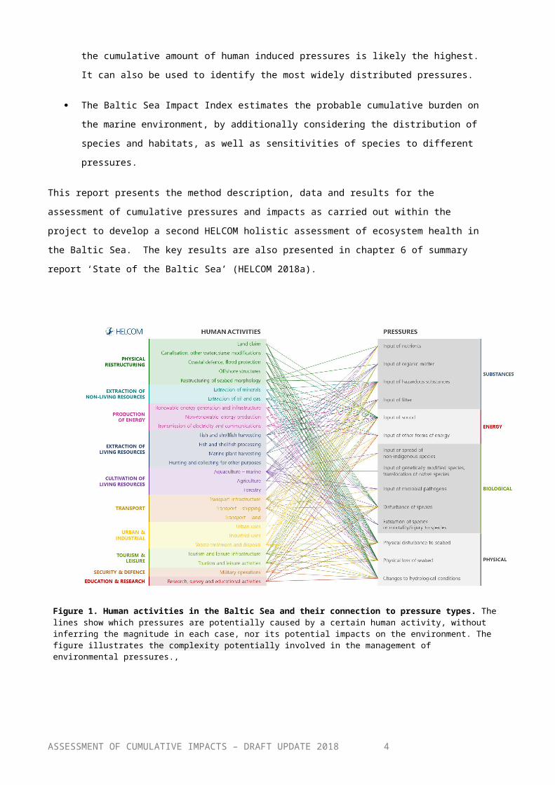
Based on their primary way of impact on the environment, pressures from human activities can be broadly categorised into four groups; inputs of substances (including nutrients, litter and contaminants, for example), inputs of energy (underwater sound, heat), biological pressures (including introduction of new species, disturbance of species and extraction of species, for example), and physical pressures (disturbance to the seabed, loss of seabed, and changes to hydrological conditions). These pressure groups are presented in figure 1, together with a comprehensive overview of human activities which can be linked to them. Some of the listed human activities are well estiablished in the Baltic Sea and its catchment area today, whereas others are more limited.

The current assessment aims to consider impacts from all human activities listed in figure 1 and occurring in the Baltic Sea during 2011-2016, as defined based on information from the countries around the Baltic Sea. The assessment is based on information on the spatial distribution of the pressures they are likely to be causing. In some cases, however, a pressure that is seen as relevant in relation to human activities has not been possible to included due to lack of data, as specified further in Chapter 2.

The results are presented in two indices:

The assessment of cumulative pressures is based on the Baltic Sea Pressure Index, which dentifies geographic areas in the Baltic Sea where the cumulative amount of human induced pressures is likely the highest. It can also be used to identify the most widely distributed pressures.

The Baltic Sea Impact Index estimates the probable cumulative burden on the marine environment, by additionally considering the distribution of species and habitats, as well as sensitivities of species to different pressures.

This report presents the method description, data and results for the assessment of cumulative pressures and impacts as carried out within the project to develop a second


HELCOM holistic assessment of ecosystem health in the Baltic Sea. The key results are also presented in chapter 6 of summary report ‘State of the Baltic Sea’ (HELCOM 2018a).

Figure 1. Human activities in the Baltic Sea and their connection to pressure types. The lines show which pressures are potentially caused by a certain human activity, without inferring the magnitude in each case, nor its potential impacts on the environment. The figure illustrates the complexity potentially involved in the management of environmental pressures.,


Chapter 2. Spatial data sets [Rewritten/new text]

The assessments were based on orginal spatial data sets for 42 human activities occurring in the Baltic Sea, and 6 data sets on pressures estimated by direct measurements at sea. These data were compiled into 18 aggregated pressure layers which were used in the Baltic Sea Pressure Index (BSPI) and the Baltic Sea Impact Index (BSII). In addition, 36 spatial data sets representing differnet ecosystem components were used in the BSII.

The layers were collated in order to generally be representative of the years 2011-2016. Data was obtained from the countries through national data calls, by enquires to the HELCOM expert projects and networks, and from the EUSeaMap project for broad-scale habitats, as explained in more detail in the HELCOM map and data service (HELCOM 2018b) and HELCOM metadatabase (HELCOM 2018c).

All spatial data was collated with the aim to be harmonized and comparable for different geographic areas of the Baltic Sea, and hence allow for a broad regional overview of pressures and impacts. The vast data collection has generally improved regional coherence in key data sets and increased the number of spatial data sets available at Baltic Sea regional scale. However, some data gaps and variation in the level of accuracy is still present when comparing difffernt data sets and geographic areas, and should be considered if examining results in more detail.

2.1 SPATIAL RESOLUTION AND SCALING[new text] The assessments were carried out at a the scale of the whole Baltic Sea, applying a spatial resolution of 1 square kilometres. Hence, orginal data sets of different types were all transformed to grid cells of 1x1km size prior to use in the analyses.

Since the original data sets were quantified in various ways, typically using different metrics and ranges of values, all values were normalised prior to the analyses in order to make them comparable with each other on a more similar scale. As a result of the normalisation, all data sets were entered with a minimum value of 0 and a maximum value of 1 in the assessments. The data sets represent continuous, ordinal and binary data, as specified in each of the metadata fact sheets.

Although it would be preferential to scale the pressures in relation to their intensity, it was not possible at this time to obtain information on relevant cutoff values for most pressure layers. Unless otherwise is indicated in the data descriptions, the lowest and highest values in each data set represent the actual range of values based on measurements, albeit normalized. Cutoffs were used when there was reason to assume that the values representing the lowest measured range were too low to likely impact on species and habitats, based on inputs from the project workshops and the HOLAS II Core Team. It should be noted, however, that this fact is ASSESSMENT OF CUMULATIVE IMPACTS – DRAFT UPDATE 2018

5

accounted for by sensitivity scores applied for estimating impacts, as they estimate sensitivities in relation to ambient conditions of the pressure at sea (Annex 2).

2.2 PRESSURE LAYERS [new texts] The pressures layers used in the assessments were defined in order to have a balance in the number of data layers representing different types of pressures. This is needed in order to prevent data-rich sectors from being over-emphaised in the results. Hence, some of the pressure layers used in the assessment are based on an aggregation of several original data sets connected to the same pressure.

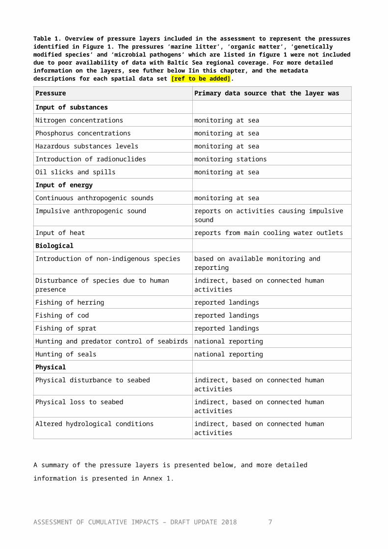
An overview of the pressure layers and their type of primary data source is presented in Table 1. Pressure data for all inputs of substances, and for continuous sound, were obtained from monitoring data representing the level of the pressure at sea. In other cases, the estimations were based on reporting on the effect of human activities. When no such direct estimates were available, the distribution of the pressures was estimated indirectly based on the connected human activities. Under this approach, the human activites mainly contributing to the pressure were back-tracked and their distribiution and potential impact distance was used as a basis for developing the aggregated pressure layers. All pressure layers were defined in order to represent the level of the pressure at sea and to be indifferent of the source of pressure.

Table 1. Overview of pressure layers included in the assessment to represent the pressures identified in Figure 1. The pressures ‘marine litter’, ‘organic matter’, ‘genetically modified species’ and ‘microbial pathogens’ which are listed in figure 1 were not included due to poor availability of data with Baltic Sea regional coverage. For more detailed information on the layers, see futher below Iin this chapter, and the metadata descriptions for each spatial data set [ref to be added].

Pressure Primary data source that the layer was based on

Input of substancesNitrogen concentrations monitoring at seaPhosphorus concentrations monitoring at seaHazardous substances levels monitoring at seaIntroduction of radionuclides monitoring stationsOil slicks and spills monitoring at seaInput of energyContinuous anthropogenic sounds monitoring at seaImpulsive anthropogenic sound reports on activities causing impulsive soundInput of heat reports from main cooling water outletsBiologicalIntroduction of non-indigenous species based on available monitoring and reportingDisturbance of species due to human presence indirect, based on connected human activitiesFishing of herring reported landingsFishing of cod reported landings


Fishing of sprat reported landingsHunting and predator control of seabirds national reportingHunting of seals national reportingPhysicalPhysical disturbance to seabed indirect, based on connected human activitiesPhysical loss to seabed indirect, based on connected human activitiesAltered hydrological conditions indirect, based on connected human activities

A summary of the pressure layers is presented below, and more detailed information is presented in Annex 1.

Pressure layers represening input of substances

Nitrogen concentrationsThe layer was interpolated from annual seasonal averages (2011-2106) of total nitrogen measured in surface waters (0-10 m), as extracted from the oceanographic databases of ICES, the Swedish Meteorological and Hydrological Institute, EEA’s Eionet database and data from Gulf of Finland year 2014. The layer was log-transformed and normalized to produce the final pressure layer. In this process, all values above the 95th and below the fifth percentile were grouped together, in order to avoid undue influence of extreme values.

Phosphorus concentrationsThe layer was interpolated from annual seasonal averages (2011-2106) of total phosphorus measured in surface waters (0-10 m), as extracted from the oceanographic databases of ICES, the Swedish Meteorological and Hydrological Institute, EEA’s Eionet database and Data from Gulf of Finland year 2014. he layer was log-transformed and normalized to produce the final pressure layer. In this process, all values above the 95th and below the fifth percentile were grouped together, in order to avoid undue influence of extreme values.

Hazardous substances levelsThe layer was interpolated based on data used in the CHASE integrated assessment of hazardosus substances, using the assessment component concentration. CHASE contamination ratios were calculated with respect to hazardous substances monitored in water, sediment and biota. The ratios were classified into five classes, values were interpolated to cover the whole Baltic Sea, and normalized to produce the final pressure layer.

Introduction of radionuclidesThe layer is based on HELCOM MORS Discharge data for 2011-2015. The isotopes taken into account were: Cesium-137, Strontium-90, and Cobalt-60. The decay-corrected annual average of the sum of radionuclide discharges (in Bequerels) was calculated for the pressure layer. A 10 km ASSESSMENT OF CUMULATIVE IMPACTS – DRAFT UPDATE 2018

7

buffer with a linearly decreasing function was used to represent the impact distance from the monitoring stations. The data set was normalized to produce the final pressure layer.

Oil slicks and spillsThe pressure layer is a combination of data sets on illegal oil discharges and polluting ship accidents. The illegal oil discharges data set is based on aerial surveillance data and on polluting ship accidents from HELOM Contracting parties’ reporting on shipping accidents. The data sets were handled separately as explained in more detail in Annex 1. They were then summed and again normalized to produce the final pressure layer.

Pressure layers represening input of energy

Continuous anthropogenic soundsThe layer was based on data from the BIAS project representing ambient underwater noise, modelled into a 0.5 km x 0.5 km grid, and representing sound pressure levels at 1/3 octave bands of 125 Hz exceeded at least 5% of the time. The data were normalized setting level 0 at 92 db re 1µPa and level 1 at 127 db re 1µPa.

Impulsive anthropogenic soundThe layer is based on the following impulsive noise events: Seismic surveys, explosions, pile driving, and air guns, as reported to the HELCOM-OSPAR Registry, hosted by ICES, and national data call. For all event types, numeric intensity values were used to represent the pressure as they are categorized in the registry (‘very low’= 0.25, ‘low’= 0.5, ‘medium’= 0.75, and ‘high’= 1). The values were used to represent the pressure intensity. No impact distance was applied due to different types of data sets included.

Input of heatThe layer is a combination of two data sets: Discharge of cooling water from nuclear power plants and from fossil fuel energy production. The data set on discharge of cooling water from nuclear power plants was obtained by direct data request to HELCOM Contracting Parties. The location of fossil fuel energy production facilities was identified and data extracted from the European Pollutant Release and Transfer Register (E-PRTR). A heat load value of 1 TWh was given to all fossil fuel production sites, based on average value for individual production sites. Heat loads from both data sets were summed and normalized to produce the final pressure layer.


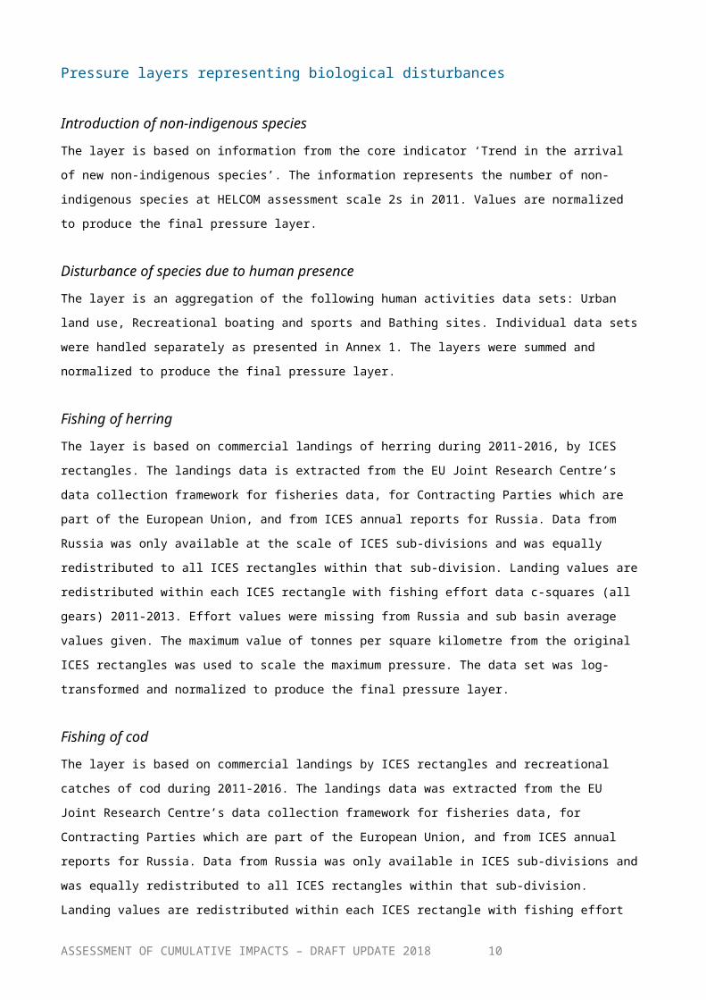
Pressure layers representing biological disturbances

Introduction of non-indigenous speciesThe layer is based on information from the core indicator ‘Trend in the arrival of new non-indigenous species’. The information represents the number of non-indigenous species at HELCOM assessment scale 2s in 2011. Values are normalized to produce the final pressure layer.

Disturbance of species due to human presenceThe layer is an aggregation of the following human activities data sets: Urban land use, Recreational boating and sports and Bathing sites. Individual data sets were handled separately as presented in Annex 1. The layers were summed and normalized to produce the final pressure layer.

Fishing of herringThe layer is based on commercial landings of herring during 2011-2016, by ICES rectangles. The landings data is extracted from the EU Joint Research Centre’s data collection framework for fisheries data, for Contracting Parties which are part of the European Union, and from ICES annual reports for Russia. Data from Russia was only available at the scale of ICES sub-divisions and was equally redistributed to all ICES rectangles within that sub-division. Landing values are redistributed within each ICES rectangle with fishing effort data c-squares (all gears) 2011-2013. Effort values were missing from Russia and sub basin average values given. The maximum value of tonnes per square kilometre from the original ICES rectangles was used to scale the maximum pressure. The data set was log-transformed and normalized to produce the final pressure layer.

Fishing of codThe layer is based on commercial landings by ICES rectangles and recreational catches of cod during 2011-2016. The landings data was extracted from the EU Joint Research Centre’s data collection framework for fisheries data, for Contracting Parties which are part of the European Union, and from ICES annual reports for Russia. Data from Russia was only available in ICES sub-divisions and was equally redistributed to all ICES rectangles within that sub-division. Landing values are redistributed within each ICES rectangle with fishing effort data c-squares (all gears) 2011-2013. Effort values were missing from Russia and sub basin average values given. The maximum value of tonnes per square kilometre from the original ICES rectangles was used to scale the maximum pressure. The Recreational data was based on data from the ICES Working Group on Recreational Fisheries Surveys (WGRFS). The data sets were summed, log-transformed and then normalized to produce the final pressure layer.


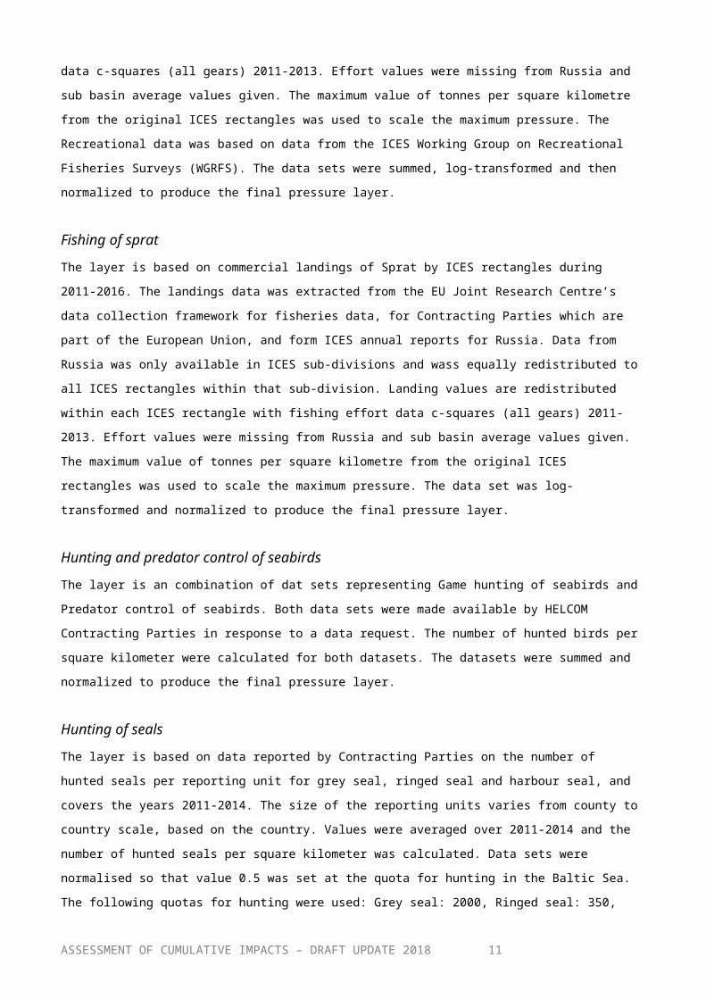
Fishing of spratThe layer is based on commercial landings of Sprat by ICES rectangles during 2011-2016. The landings data was extracted from the EU Joint Research Centre’s data collection framework for fisheries data, for Contracting Parties which are part of the European Union, and form ICES annual reports for Russia. Data from Russia was only available in ICES sub-divisions and wass equally redistributed to all ICES rectangles within that sub-division. Landing values are redistributed within each ICES rectangle with fishing effort data c-squares (all gears) 2011-2013. Effort values were missing from Russia and sub basin average values given. The maximum value of tonnes per square kilometre from the original ICES rectangles was used to scale the maximum pressure. The data set was log-transformed and normalized to produce the final pressure layer.

Hunting and predator control of seabirdsThe layer is an combination of dat sets representing Game hunting of seabirds and Predator control of seabirds. Both data sets were made available by HELCOM Contracting Parties in response to a data request. The number of hunted birds per square kilometer were calculated for both datasets. The datasets were summed and normalized to produce the final pressure layer.

Hunting of sealsThe layer is based on data reported by Contracting Parties on the number of hunted seals per reporting unit for grey seal, ringed seal and harbour seal, and covers the years 2011-2014. The size of the reporting units varies from county to country scale, based on the country. Values were averaged over 2011-2014 and the number of hunted seals per square kilometer was calculated. Data sets were normalised so that value 0.5 was set at the quota for hunting in the Baltic Sea. The following quotas for hunting were used: Grey seal: 2000, Ringed seal: 350, Harbour seal 230. The datasets were normalized to produce the final pressure layer.

Pressure layers representing physical disturbances

Physical disturbance to seabedPhysical disturbance was defined as a change to the seabed which can be reverted if the activity causing the disturbance ceases (EC 2017a). The activities included in the spatial layer representing physical disturbance were cables, coastal defence and flood protection, deposit of dredged material, dredging, extraction of sand and gravel, finfish mariculture, furcellaria harvesting, pipelines, recreational boating and sports, scallop and blue mussel dredging, shellfish mariculture and wind farms (acting via the pressures of siltation, smothering, and abrasion), and in addition shipping and trawling were included as potentially causing physical disturbance.


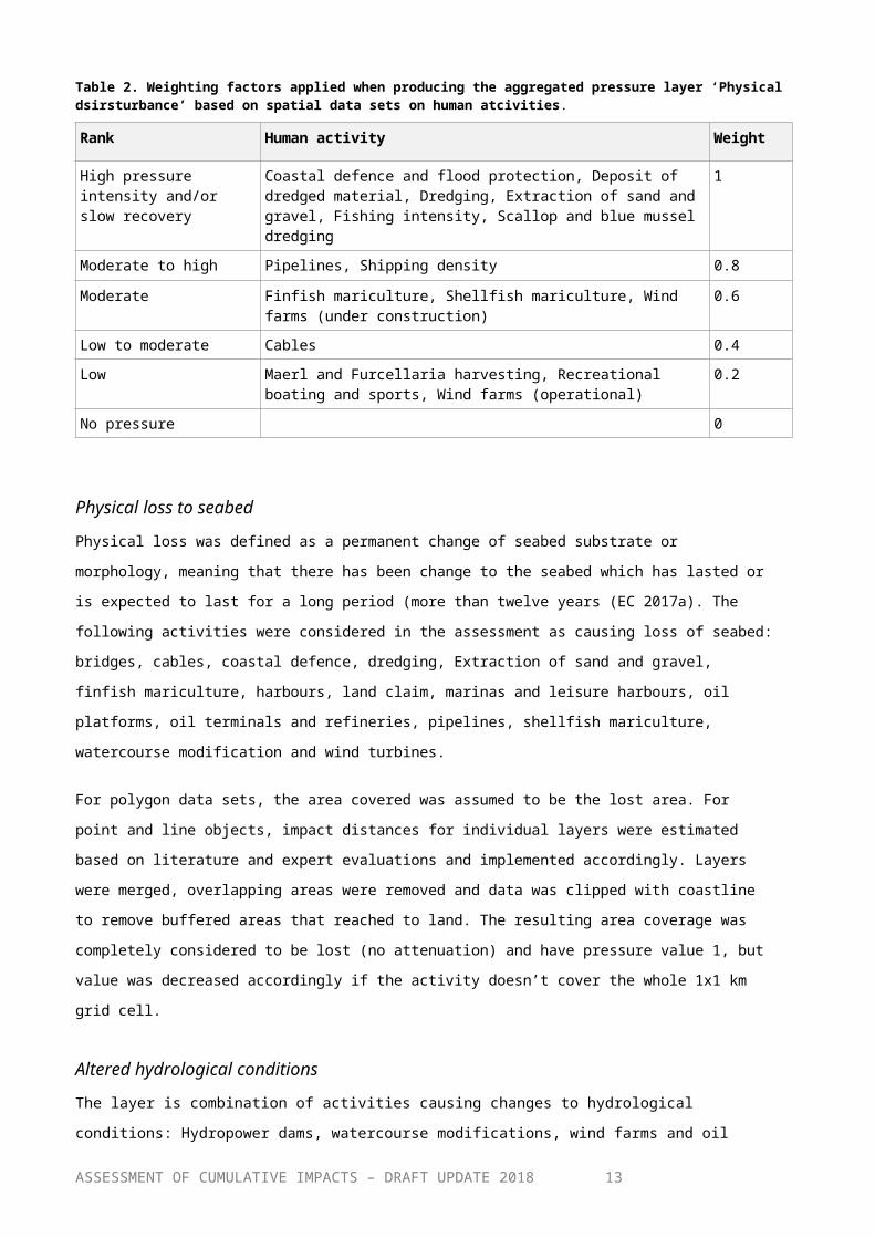
Impact distances and attenuation gradients for individual human activities layers were estimated based on literature and expert evaluations and implemented accordingly (Annex 1). Weighting factors were applied to all individual layers to account for the relative difference in the intensity of the pressures (See Table 2 for the weighting factors used). The layers were summed together and normalized to produce the final pressure layer.


Table 2. Weighting factors applied when producing the aggregated pressure layer ‘Physical dsirsturbance’ based on spatial data sets on human atcivities.

Rank Human activity Weight

High pressure intensity and/or slow recovery

Coastal defence and flood protection, Deposit of dredged material, Dredging, Extraction of sand and gravel, Fishing intensity, Scallop and blue mussel dredging

1

Moderate to high Pipelines, Shipping density 0.8Moderate Finfish mariculture, Shellfish mariculture, Wind farms (under

construction)0.6

Low to moderate Cables 0.4Low Maerl and Furcellaria harvesting, Recreational boating and

sports, Wind farms (operational)0.2

No pressure 0

Physical loss to seabedPhysical loss was defined as a permanent change of seabed substrate or morphology, meaning that there has been change to the seabed which has lasted or is expected to last for a long period (more than twelve years (EC 2017a). The following activities were considered in the assessment as causing loss of seabed: bridges, cables, coastal defence, dredging, Extraction of sand and gravel, finfish mariculture, harbours, land claim, marinas and leisure harbours, oil platforms, oil terminals and refineries, pipelines, shellfish mariculture, watercourse modification and wind turbines.

For polygon data sets, the area covered was assumed to be the lost area. For point and line objects, impact distances for individual layers were estimated based on literature and expert evaluations and implemented accordingly. Layers were merged, overlapping areas were removed and data was clipped with coastline to remove buffered areas that reached to land. The resulting area coverage was completely considered to be lost (no attenuation) and have pressure value 1, but value was decreased accordingly if the activity doesn’t cover the whole 1x1 km grid cell.

Altered hydrological conditionsThe layer is combination of activities causing changes to hydrological conditions: Hydropower dams, watercourse modifications, wind farms and oil platforms. Impact distances and attenuation gradients for individual human activities were estimated based on literature and expert evaluations and implemented accordingly. Data sets were handled separately, summed together and overlapping areas were removed to avoid double counting. Layer was normalized to produce the final pressure layer.


2.4 HUMAN ACTIVITIES POTENTIALLY ATTRIBUTED TO SEABED LOSS AND DISTURBANCE[This section on the human activites potentially attributed to seabed loss and disturbance is suggested to be presented as a separate layout element, for example over two pages with different background color (or a “box”). The text is is identifical to that on seabed loss and disturbance in the summary report chapter 4.7]

Several human activities may cause severe damage to benthic habitats and species, some by direct contact with the seabed and others through indirect effects caused by the increased turbidity or sedimentation, for example. Whether an activity leads to a permanent loss or a temporary disturbance of benthic habitats depends on many factors such as the duration and intensity of the activity, the technique used, and the sensitivity of the area affected. The loss of a natural habitat may give rise to a new artificial habitat, for example when a construction creates rocky bottoms on sand. This may also lead to ecological changes that are undesirable.

Many activities may contribute to both permanent loss and disturbance of the seabed (Figure 2). Hence, estimating seabed loss and physical disturbance at a regional and sub-basin scale requires a generalised approach which links together different types of activities with potential loss and disturbance of the seabed and thereby simplifies the complex reality.

[new/moved].A summary of the principal human activities connected to seabed loss and disturbance is provided below, based on Figure 2. Whether an activity in reality leads to loss of or disturbance of habitats depends on many factors, such as the duration and intensity of the activity, the technique used and the sensitivity of the area affected. The identification of which activities lead to loss and/or physical disturbance is still under development

In addition, physical disturbance may be exptressed as modification of hydrological conditiion. The human activitity most likely to influence on hydrological conditions in the Baltic Sea is the presence of off shore wind farms, whereas other construction in the open sea have clearly lower spatial extent.


Figure 2 Generalised overview of human activity types and the physical pressures they may exert on the seabed. The pressures are further grouped into those causing loss and disturbance of the seabed. Black lines link to potential physical loss of seabed habitats, and blue lines link to potential physical disturbance. Smothering is linked to disturbance in the graph, but may in some cases also lead to loss, depending on tolerance of the impacted organisms and intensity of the pressure.

Construction and installationsOff-shore wind farms, harbours and underwater cables and pipelines are examples of constructions that cause a local but permanent loss of habitat. In addition, disturbance to the seabed may occur during the period of construction and installation. The pressures exerted during the construction phase are in some instances similar to those during sea-bed extraction or dredging into the seabed (see below).

Installation of off-shore construction may in some cases also encompass drilling or the relocation of substrate for use as scour protection. The area lost by scour protection around the foundation of a wind farm turbine has been estimated to be in the order of 20 meters from the wind turbine (OSPAR 2008). The scour protection will give rise to a new man-made habitat.

Cables and pipelines may be placed in a trench and then covered with sediment extracted elsewhere. Most often the sediment composition then differs from surrounding habitats (Schwarzer et al. 2014). On hard substrates, cables are often covered with a protective layer of steel or concrete casings. The loss of habitats by smothering and sealing from cables has been generalised to a 2 meters distance for the assessment purposes (OSPAR 2008).

Open systems of mariculture affect the seabed habitat through sedimentation of excrements under the fish and shellfish farms, as the accumulated material changes the seabed substrate. However, the extent of the effects in terms of loss and disturbance depends on the hydrological conditions and on the properties of the mariculture, and currently no information exists on the recovery rate when the pressure is removed.


DredgingDredging activities are usually divided into capital dredging, which is carried out when building new constructions, and maintenance dredging, which is done in order to maintain existing waterways.

Dredging causes different types of pressure on the sea bed; removal of substrate alters physical conditions through changes in the seabed topography, increased turbidity caused by re-suspended fine sediments, and smothering and siltation of nearby areas due to settling of suspended load. Loss of habitat occurs during capital dredging which usually is a pressure occurring once at a specific location. But loss of habitat also occurs during maintenance dredging which is performed repeatedly, often at regular intervals. The loss is limited to the dredging site, whilst disturbance through sedimentation may have a wider spatial extent.

Some studies have estimated that disturbance through sedimentation may affect animals and vegetation up to a couple of kilometres from the core activity (Lassalle et al. 1990, Boyd et al. 2003, Orviku et al. 2008). In addition, remobilisation of sediments with deposited substances may contribute to contamination and eutrophication effects.

Sand and gravel extractionDuring sand and gravel extraction sediment is removed from the seabed, for use in construction, coastal protection, beach nourishment and land-fills, for example.

Sand and gravel extraction can be performed using either static dredging or trailer dredging. When using static dredging, the pressures exerted by sand and gravel extraction are comparable to those during dredging; potential physical loss of habitat (which may be partial or complete depending on how much sand or gravel is removed and which extraction technique is used), altered physical conditions through changes in seabed topography, increased turbidity caused by fine sediments that are mobilised into the water, or smothering or siltation on nearby areas. When performing trailer dredging the pressures exerted are more limited. In addition, in areas where the sediment mobility and dynamics are naturally high, the effects of sand and gravel extraction may be less significant.

Since the extracted material is sieved at sea to the wanted grain size, the unwanted matter is discharged and may result in a changed grain size of the local sediment on the seabed. Sedimentation levels are more restricted during sand and gravel extraction than during dredging, and may occur a few hundred metres from the core activity (Newell et al. 1998). There is more or less full mortality of benthic organisms at the site of sand and gravel extraction as they are removed together with their habitat (Boyd et al. 2000, 2003, Barrio Frojan et al. 2008), whereas the extent of the impact on adjacent areas is smaller (Vatanen et al. 2010).

Importantly, there are modern techniques and concepts which, if applied, can help to reduce the negative impact. Recolonization by sand- and gravel dwelling organisms is for example


facilitated if the substrate is not completely removed. Precautionary measures are also recommended in HELCOM Recommendation 19/1 on ‘Marine Sediment Extraction in the Baltic Sea Area’.

Disposal of dredged matterDisposal of dredged matter may cause covering of the seabed, smothering of benthic organisms, and lead to loss of habitat if the sediment characteristics are changed. In addition, increased turbidity during the disposal cause increased siltation on the site itself and in the areas around it. Disposed material may contain higher concentrations of hazardous substances and nutrients than the disposal site and may cause accumulation of these pollutants at the disposal site and adjacent areas.

The impacts on the species depend mainly on the seabed habitat type, the type and amount of disposed material, and distance to the disposal site. Burial of benthic organisms may cause mortality, but some species have the ability to re-surface (Olenin 1992, Powilleit et al. 2009). The probability of survival is higher on soft bottoms, whereas vegetation and fauna on hard substrates die when covered by a few centimetres of sediment (Powilleit et al. 2009, Essink 1999). The spatial extent of the impacts is similar to that of dredging a couple of kilometres from the core zone of the activity (Syväranta and Leinikki 2015, Vatanen et al. 2015).

ShippingShip traffic can cause disturbance to the seabed in several ways; propeller induced currents may cause abrasion, resuspension and siltation of sediments, shipbow waves may cause stress to littoral habitats, and dragging of anchors may cause direct physical disturbance to the seabed.

Disturbances to the seabed from shipping mainly occur in shallow areas. The effects are often local, concentrated to shipping lanes and to the vicinity of harbours. For larger vessels, increased turbidity has been observed down to 30 m depth (Vatanen et al. 2010), and mid-sized ferry traffic has been estimated to increase turbidity by 55 % in small inlets (Eriksson et al. 2004). Erosion of the sea-floor can be substantial along heavy shipping lanes, and has been observed to cause up to 1 m of sediment loss due to abrasion (Rytkönen et al. 2001).

Bottom trawlingBottom contacting fishing gear causes surface abrasion. During bottom trawling it may also reach deeper down into the sediment, causing subsurface abrasion to the seabed.

The substrate that is swept by bottom trawling is affected by temporary disturbance, and bottom dwelling species are removed from the habitat or relocated (Dayton et al. 1995). The impact is particularly strong on slow growing sessile species which may be eradicated. Since the same areas are typically swept repeatedly, and due to high density of trawling in some areas,


the possibility to recover may also be low for more resilient organisms, and a change in species composition may be seen (Kaiser et al. 2006, Olsgaard et al. 2008).

In addition, the activity may mobilise sediments into the water, which may be transported to other areas and cause smothering on hard substrates, or may release hazardous substances that have been previously buried in the seabed (Jones 1992, Wikström et al. 2016).

The estimate of disturbance from fishing used in this evaluation is based on fishing intensity calculated by ICES (International council for exploration of the sea), based on data from the vessel monitoring system on the location of fishing vessels complemented with logbook information.


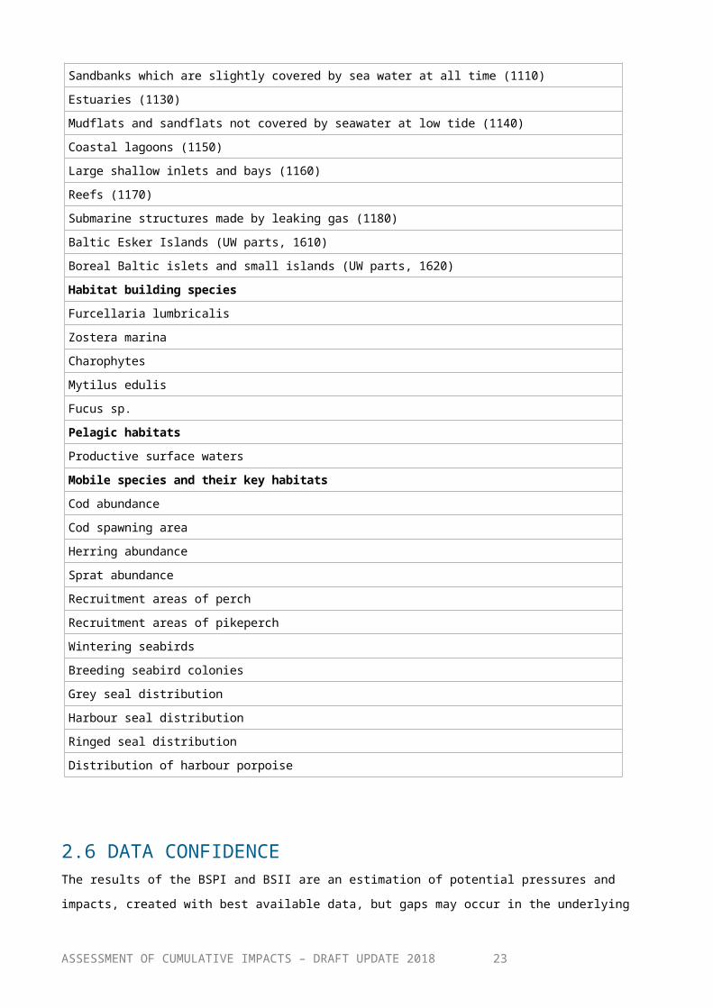
2.5. ECOSYSTEM COMPONENT LAYERSThe data sets on ecosystem components, which were additionally used in the Baltci Sea Impact index, are presented in Table 3. The ecosystem component data sets represent the spatial distribution of habitats and species with high ecological importance in the Baltic Sea, for which data was available and comparable at the Baltic Sea regional scale. The following groups were included 1) benthic habitats based on the EMODnet broad-scale habitats and Natura 2000 habitats, 2) habitat-building species, 3) pelagic habitats defined as the photic surface layer and the layer beneath, 4) mobile species (mammals, birds and fish species characteristic species for the Baltic Sea, as well as the habitats they use.

Simlar as for the pressure layers, the ecosystem component data sets were defined to represent the situation during 2011-2016. Hence, they do not include information on where species would occur had there been no historical pressures from human activities. For example, the distribution of cod spawning areas is shown based on information on currently functional spawning areas, which have a clearly more limited distribution compared to the past (Köster et al. 2017). Hence, the assessment focuses on identifying current potential impacts, given the existing status of species and habitats.

Table 3. Ecosystem component layers included in the assessment. The layers were based on data collected from various sources, including national data calls and input from HELCOM expert groups For more detailed information on the layers, see futher below Iin this chapter, and the metadata descriptions for each spatial data set [ref to be added]

Ecosystem component

Benthic habitatsOxygenated deep watersInfralittoral hard bottomInfralittoral sandInfralittoral mudInfralittoral mixedCircalittoral hard bottomCircalittoral sandCircalittoral mudCircalittoral mixedSandbanks which are slightly covered by sea water at all time (1110)Estuaries (1130)Mudflats and sandflats not covered by seawater at low tide (1140)Coastal lagoons (1150)Large shallow inlets and bays (1160)Reefs (1170)Submarine structures made by leaking gas (1180)


Baltic Esker Islands (UW parts, 1610)Boreal Baltic islets and small islands (UW parts, 1620)Habitat building speciesFurcellaria lumbricalis Zostera marinaCharophytes Mytilus edulisFucus sp.Pelagic habitatsProductive surface watersMobile species and their key habitatsCod abundance Cod spawning area Herring abundance Sprat abundance Recruitment areas of perchRecruitment areas of pikeperch Wintering seabirdsBreeding seabird coloniesGrey seal distributionHarbour seal distributionRinged seal distributionDistribution of harbour porpoise

2.6 DATA CONFIDENCE The results of the BSPI and BSII are an estimation of potential pressures and impacts, created with best available data, but gaps may occur in the underlying datasets. Thus, areas with low impact may imply data gaps and different areas cannot be directly compared at this time. The underlying datasets and metadata can be viewed and downloaded from the HELCOM map and data service.

[to be elaborated further]

2.7 CONNECTION TO THE MARINE STRATEGY FRAMEWORK DIRECTIVEThe organization of the pressure layers used is in line with Annex III of the revised the Marine Strategy Framework Directive (EC 2017 a, b). Some modifications were applied to make the list applicable to Baltic Sea conditions. Human activities not occurring in the Baltic Sea were ASSESSMENT OF CUMULATIVE IMPACTS – DRAFT UPDATE 2018

19

omitted, and some pressures were sub-divided as they were considered important for the region: fishing was subdivided into fishing on different species, hunting of seals and seabirds are assessed separately, and inputs of nitrogen and phosphorus were assessed separately.

Climate change related pressures – acidification and changes in salinity and temperature - were not included due to a lack of approach for how to handle the monitoring data. Furthermore, data on the inputs of litter and organic matter were not included due to a lack of spatial information.


Chapter 3. Method for the assessment of cumulative pressures and impacts [same content as before, edited] The Baltic Sea Impact Index (BSII) was first applied in the Initial HELCOM Holistic assessment (HELCOM 2010a), building on concepts described by Halpern et al. (2008). The methods that were applied then are described by HELCOM (2010b) and Korpinen et al. (2012). The concepts were subsequently developed further for parts of the North Sea area in the HARMONY project (Andersen et al. 2013), which also developed an assessment software (Stock 2016). The same methodology has also been used in the Mediterranean and the Black Sea (Micheli et al. 2013).

However, although the method used in the ‘State of the Baltic Sea report’ (HELCOM 2018a) is similar to that applied in HELCOM (2010a), the assessment approach has been refined with a focus on improving the data underlying the assessment, and the structure how the data layers were included has been changed in order to provided a more balanced assessment. Hence, results form HELCOM (2010s) can not be directly be compared to the results presented here in quantitative terms.

3.1 ASSESSMENT TOOL The assessment was carried out in an ArcGIS toolbox particulary designed and created for this purpose at the HELCOM Secretariat. The tool uses the same principles as the EcoImpactMapper software, but is run in a spatial framework, and is flexible for being further developed and modified according to future needs. The developed tool can exploit directly the pressure and ecosystem component layers without conversion and automatically integrates the sensitivirty scores to this process.

3.2 CALCULATION OF BSII AND BSPI [same content as before, edited] Both the Baltic Sea Pressure Index and the Baltic Sea Impact Index were carried out at a full Baltic Sea regional scale based on assessment units of 1 square kilometres (grid cells).

The key components of the Baltic Sea Impact Index (BSII) are georeferenced data sets of human induced pressures and ecosystem components, as well as sensitivity scores that are used in combining the pressure and ecosystem component layers. The sensitivity scores estimate the potential impact of each assessed pressure on each specific ecosystem component, and were defined as presented further below (Chapter 3.5)

The Impact Index was calculated based on the sum of all impacts in one assessment unit, for all ecosystem components, as shown in formula A (where D=the pressures, n= the number of


pressures, e= ecosystem components, m=the number of ecosystem components, and µ =the sensitivity of each ecosystem component to each pressure):

(A)

The Baltic Sea Pressure Index was calculated without considering the values of ecosystem components, but including the average sensitivity score of all ecosystem component to individual pressure (formula B). This analysis gives the cumulative anthropogenic pressures in each grid cell calibrated with the mean sensitivity score to each pressure.

(B)

3.3 CONFIDENCE IN THE ASSESSMENT[rewritten] The overall confidence in the assessment is to be evaluated qualitatively, by examination of the underlying spatial data sets and sensitivity scores. An quantatiative evaluation of confidence in the BSII and BSPI assessments was not made.

One limitation, currenly, to a quantative assessment is that manu data sets only include information on which activities or pressures are present, while the absence of information may reflect either a true absence or missing data In particular, the assessment of potential loss and disturbance can be underestimated in some sub-basins due to lack of data of human actitivities connected to this pressures. For examining this aspext, the spatial data stes on human activities underlying the assessment should be evaluated qualitatively.

The relative role of the sensitivity scores in influencing the outcome can be elevated if the assessment is based on only a limited number of spatial data sets (Korpinen et al. 2012). The current assessment is not seen as limited in this respect.

The assessment is based on additive effects. However, in reality impacts may also be synergistic (or antagonistic), so that the total effect of many pressures can be larger (or higher) than the sum due to interactions in the food web and ecosystem feedbacks. The current version of the BSII does not take such more complex linkages into account.

The BSII is designed to evaluate spatial aspects, identifiying areas where human induced pressures are likely to have relatively high or low cumulative impact on the marine environment. Hence, results for particular areas are to be compared to that of other areas in relative terms.


3.4 METHOD IMPLICATIONS[new]

The applied approach allows for including several ecosystem component layers per grid cell and is suitable when the underlying ecosystem component data sets have relatively high level of detail, as is the case in the current assessment.

The Baltic Sea Impact Index was assessed based on the ‘sum impact’ because, compared to other computation options, the sum approach gives a greater range of high and low impact values and hence distinguishes patterns more clearly.

In cases where there are significant gaps in the underlying ecosystem component data sets, it may be more suitable to use the method of ‘average impact’ or ‘maximum impact’. The ‘average impact’ has been used in assessments in other sea areas such the California Current (e.g. Halpern et al. 2015). The ‘maximum impact’ method might be appropriate to highlight areas of high risk.

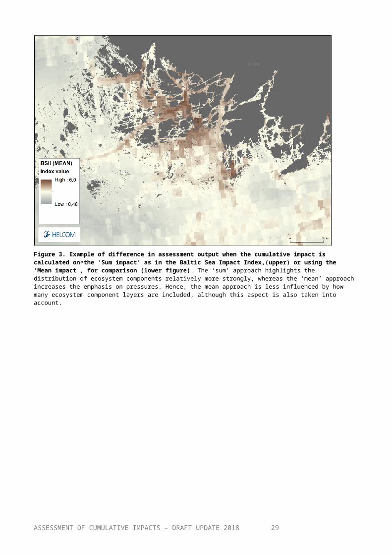
One implication of using the ‘sum’ approach, as applied here, is that the overall assessment outcome depends on the number of ecosystem components and pressures assessed in each grid cell. The highest impacts are often observed in assessment units where several pressures and/or ecosystem components are present. Therefore, a high index score can either be explained by the impact of several pressures, or by the impact of a single pressure on several ecosystem components (Figure 3).


Figure 3. Example of difference in assessment output when the cumulative impact is calculated on the ‘Sum impact’ as in the Baltic Sea Impact Index,(upper) or using the ‘Mean impact”, for comparison (lower figure). The ‘sum’ approach highlights the distribution of ecosystem components relatively more strongly, whereas the ‘mean’ approach increases the emphasis on pressures. Hence, the mean approach is less influenced by how many ecosystem component layers are included, although this aspect is also taken into account.


3.5 SENSITIVITY SCORES[rewritten, no new content] The sensitivity scores estimate the sensitivity of species and habitats to the different pressures, and is used in the Baltic sea Impct Index (Formula A in Chapter 3.2).

The sensitivity score used in this assessment were obtained from a survey answered by over eighty experts in the Baltic Sea region, representing marine research and management authorities in seven Baltic Sea countries. The results were evaluated for compatibility with a literature review study on physical loss and disturbance of benthic habitats, and assessed in relation to a self-evaluation of the experts on their confidence in their replies. These steps are defined in more detail further below.

Sensitivity scores for assessing impacts on benthic habitats and species were also based on a literature review provided by the BalticBOOST project. The literature review assessed the sensitivity of all kinds of benthic habitats to the pressures physical loss, physical disturbance and changes in hydrological conditions. The review suggested that the pressure ‘physical loss’ is given the highest sensitivity score in all cases. The literature that was used to suggests sensitivity scores for the pressures ‘physical disturbance’ and that for ‘hydrological conditions’ are presented in Annex 1, which also lists literature to support the setting of sensitivity score of benthic habitats for other pressures, as well as other literature referred.

The sensitivity scores finally applied in the assessment are presented in table 4, for each combination of ecosystem components and pressures.


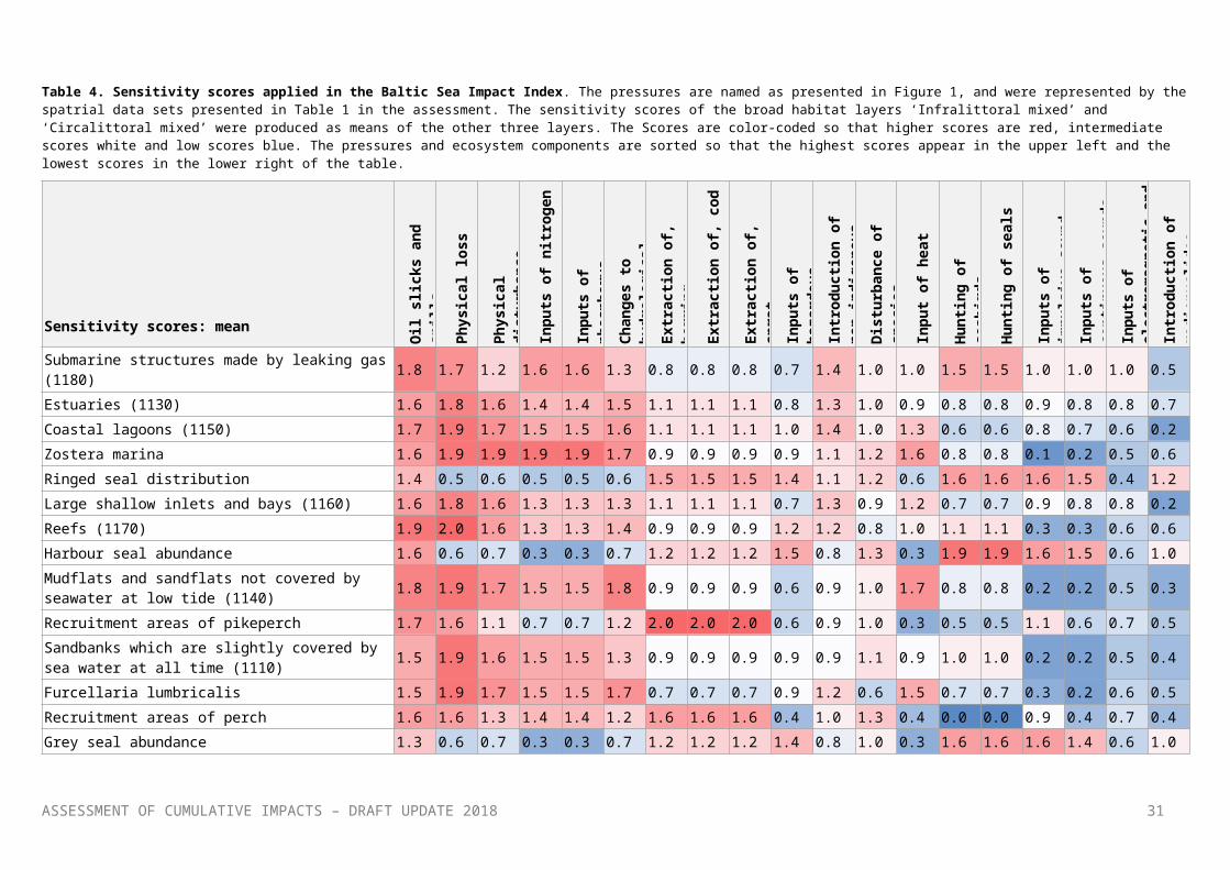
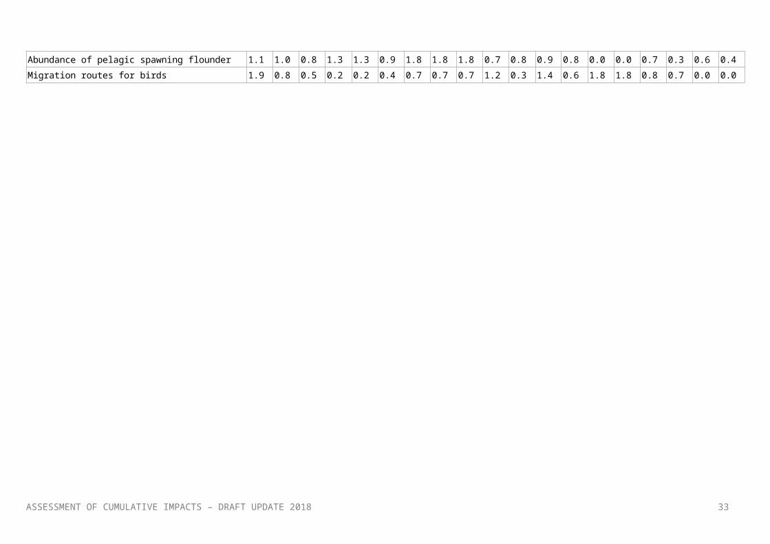
Table 4. Sensitivity scores applied in the Baltic Sea Impact Index. The pressures are named as presented in Figure 1, and were represented by the spatrial data sets presented in Table 1 in the assessment. The sensitivity scores of the broad habitat layers ‘Infralittoral mixed’ and ‘Circalittoral mixed’ were produced as means of the other three layers. The Scores are color-coded so that higher scores are red, intermediate scores white and low scores blue. The pressures and ecosystem components are sorted so that the highest scores appear in the upper left and the lowest scores in the lower right of the table.

Sensitivity scores: mean

Oil

slic

ks a

nd s

pills

Phys

ical

loss

Phys

ical

di

stur

banc

e

Inpu

ts o

f nitr

ogen

Inpu

ts o

f ph

osph

orus

Chan

ges

to

hydr

olog

ical

Ex

trac

tion

of,

herr

ing

Extr

actio

n of

, cod

Extr

actio

n of

, spr

at

Inpu

ts o

f haz

ardo

us

subs

tanc

esIn

trod

uctio

n of

no

n-in

dige

nous

D

istu

rban

ce o

f sp

ecie

s

Inpu

t of

hea

t

Hun

ting

of s

eabi

rds

Hun

ting

of s

eals

Inpu

ts o

f im

puls

ive

soun

dIn

puts

of

cont

inuo

us s

ound

s In

puts

of

elec

trom

agne

tic

Intr

oduc

tion

of

radi

onuc

lides

Submarine structures made by leaking gas (1180) 1.8 1.7 1.2 1.6 1.6 1.3 0.8 0.8 0.8 0.7 1.4 1.0 1.0 1.5 1.5 1.0 1.0 1.0 0.5Estuaries (1130) 1.6 1.8 1.6 1.4 1.4 1.5 1.1 1.1 1.1 0.8 1.3 1.0 0.9 0.8 0.8 0.9 0.8 0.8 0.7Coastal lagoons (1150) 1.7 1.9 1.7 1.5 1.5 1.6 1.1 1.1 1.1 1.0 1.4 1.0 1.3 0.6 0.6 0.8 0.7 0.6 0.2Zostera marina 1.6 1.9 1.9 1.9 1.9 1.7 0.9 0.9 0.9 0.9 1.1 1.2 1.6 0.8 0.8 0.1 0.2 0.5 0.6Ringed seal distribution 1.4 0.5 0.6 0.5 0.5 0.6 1.5 1.5 1.5 1.4 1.1 1.2 0.6 1.6 1.6 1.6 1.5 0.4 1.2Large shallow inlets and bays (1160) 1.6 1.8 1.6 1.3 1.3 1.3 1.1 1.1 1.1 0.7 1.3 0.9 1.2 0.7 0.7 0.9 0.8 0.8 0.2Reefs (1170) 1.9 2.0 1.6 1.3 1.3 1.4 0.9 0.9 0.9 1.2 1.2 0.8 1.0 1.1 1.1 0.3 0.3 0.6 0.6Harbour seal abundance 1.6 0.6 0.7 0.3 0.3 0.7 1.2 1.2 1.2 1.5 0.8 1.3 0.3 1.9 1.9 1.6 1.5 0.6 1.0Mudflats and sandflats not covered by seawater at low tide (1140) 1.8 1.9 1.7 1.5 1.5 1.8 0.9 0.9 0.9 0.6 0.9 1.0 1.7 0.8 0.8 0.2 0.2 0.5 0.3Recruitment areas of pikeperch 1.7 1.6 1.1 0.7 0.7 1.2 2.0 2.0 2.0 0.6 0.9 1.0 0.3 0.5 0.5 1.1 0.6 0.7 0.5Sandbanks which are slightly covered by sea water at all time (1110) 1.5 1.9 1.6 1.5 1.5 1.3 0.9 0.9 0.9 0.9 0.9 1.1 0.9 1.0 1.0 0.2 0.2 0.5 0.4Furcellaria lumbricalis 1.5 1.9 1.7 1.5 1.5 1.7 0.7 0.7 0.7 0.9 1.2 0.6 1.5 0.7 0.7 0.3 0.2 0.6 0.5Recruitment areas of perch 1.6 1.6 1.3 1.4 1.4 1.2 1.6 1.6 1.6 0.4 1.0 1.3 0.4 0.0 0.0 0.9 0.4 0.7 0.4Grey seal abundance 1.3 0.6 0.7 0.3 0.3 0.7 1.2 1.2 1.2 1.4 0.8 1.0 0.3 1.6 1.6 1.6 1.4 0.6 1.0Charophytes 1.5 1.9 1.9 1.7 1.7 1.4 0.8 0.8 0.8 0.8 1.4 0.7 0.9 0.7 0.7 0.0 0.0 0.6 0.4Circalittoral hard bottom 1.3 1.9 1.3 1.3 1.3 1.4 0.8 0.8 0.8 1.2 1.2 0.4 1.2 1.0 1.0 0.3 0.3 0.6 0.5Wintering seabirds 2.0 0.9 0.8 0.2 0.2 0.5 1.1 1.1 1.1 1.4 0.6 1.3 0.4 1.7 1.7 0.9 0.8 0.6 0.7Distribution of harbour porpoise 1.6 1.2 1.3 0.2 0.2 0.4 1.5 1.5 1.5 1.6 0.4 1.2 0.5 0.0 0.0 1.9 1.7 0.3 1.0

ASSESSMENT OF CUMULATIVE IMPACTS – DRAFT UPDATE 2018 26

Baltic Esker Islands (UW parts, 1610) 1.6 1.8 1.5 1.3 1.3 1.3 0.8 0.8 0.8 0.8 1.3 0.7 1.0 0.5 0.5 0.5 0.5 0.5 0.1Boreal Baltic islets and small islands (UW parts, 1620) 1.6 1.8 1.5 1.2 1.2 1.1 0.8 0.8 0.8 0.8 1.3 0.7 1.0 0.5 0.5 0.5 0.5 0.5 0.1Breeding seabird colonies 2.0 0.9 0.9 0.3 0.3 0.4 1.0 1.0 1.0 1.3 0.8 1.8 0.3 1.6 1.6 0.8 0.6 0.3 0.2Cod abundance 0.5 1.0 0.7 1.5 1.5 0.4 1.6 1.6 1.6 0.8 0.6 0.9 0.7 0.7 0.7 0.9 0.2 0.5 0.6Infralittoral hard bottom 1.7 1.8 1.3 1.3 1.3 1.2 0.6 0.6 0.6 1.0 1.1 0.3 1.3 0.7 0.7 0.2 0.2 0.6 0.4Fucus sp. 1.4 1.8 1.7 1.3 1.3 1.3 0.5 0.5 0.5 0.9 1.2 0.6 1.5 0.3 0.3 0.3 0.3 0.5 0.5Cod spawning area 1.0 0.7 0.8 1.7 1.7 0.9 1.3 1.3 1.3 0.9 0.4 0.6 0.6 0.2 0.2 1.0 0.6 0.5 0.5Productive surface waters 1.4 0.4 1.0 1.5 1.5 0.6 1.0 1.0 1.0 1.0 1.0 0.8 1.0 0.5 0.5 0.6 0.6 0.4 0.0Circalittoral mixed 1.1 1.8 1.1 1.2 1.2 1.3 0.6 0.6 0.6 1.0 1.0 0.4 0.9 0.7 0.7 0.3 0.3 0.6 0.4Infralittoral mixed 1.5 1.8 1.2 1.3 1.3 1.1 0.4 0.4 0.4 1.0 1.0 0.3 1.1 0.7 0.7 0.3 0.3 0.6 0.3Circalittoral mud 1.1 1.6 1.0 1.2 1.2 1.3 0.6 0.6 0.6 1.0 0.9 0.4 0.9 0.5 0.5 0.3 0.3 0.8 0.5Mytilus edulis 1.6 1.8 1.6 0.9 0.9 1.6 0.4 0.4 0.4 1.1 1.4 0.4 1.0 0.2 0.2 0.1 0.2 0.5 0.5Infralittoral mud 1.4 1.7 1.1 1.3 1.3 1.1 0.3 0.3 0.3 1.0 0.9 0.4 1.0 0.7 0.7 0.3 0.3 0.6 0.4Infralittoral sand 1.4 1.8 1.2 1.3 1.3 0.9 0.3 0.3 0.3 0.9 0.9 0.3 1.0 0.7 0.7 0.3 0.3 0.5 0.2Oxygenated deep waters 1.0 0.9 0.7 1.8 1.8 1.3 0.7 0.7 0.7 0.9 0.7 0.2 0.6 0.3 0.3 0.6 0.5 0.5 0.0Circalittoral sand 0.9 1.8 1.1 1.2 1.2 1.1 0.3 0.3 0.3 0.9 1.0 0.3 0.7 0.7 0.7 0.3 0.2 0.5 0.2Herring abundance 0.9 0.9 0.7 0.7 0.7 0.7 1.2 1.2 1.2 0.4 0.6 0.4 0.6 0.2 0.2 1.1 0.6 0.5 0.3Sprat abundance 0.9 0.5 0.5 0.6 0.6 0.7 1.2 1.2 1.2 0.4 0.6 0.4 0.6 0.2 0.2 1.1 0.6 0.5 0.3Scores for layers that were finally not includedHarbour seal haulouts 1.6 0.8 0.9 0.3 0.3 0.6 1.0 1.0 1.0 1.6 0.5 1.6 0.2 2.0 2.0 1.5 1.5 0.3 0.3Grey seal haulouts 1.4 0.8 0.9 0.3 0.3 0.6 1.0 1.0 1.0 1.6 0.5 1.4 0.2 2.0 2.0 1.5 1.5 0.3 0.3Recruitment areas of roach 1.7 1.7 1.1 0.5 0.5 1.2 1.6 1.6 1.6 0.6 0.9 0.8 0.3 0.5 0.5 1.0 0.6 0.4 0.5Abundance of pelagic spawning flounder 1.1 1.0 0.8 1.3 1.3 0.9 1.8 1.8 1.8 0.7 0.8 0.9 0.8 0.0 0.0 0.7 0.3 0.6 0.4Migration routes for birds 1.9 0.8 0.5 0.2 0.2 0.4 0.7 0.7 0.7 1.2 0.3 1.4 0.6 1.8 1.8 0.8 0.7 0.0 0.0

ASSESSMENT OF CUMULATIVE IMPACTS – DRAFT UPDATE 2018 27

Design of the expert surveyThe expert survey was developed in the TAPAS project and was presented in Microsoft Excel, supplemented with guidance on how to respond to the survey (Annex 1).

The survey contained a matrix of all possible combinations of pressures and ecosystem components, in the same format as was shown in Table 4. Respondents were asked to provide estimates with respect to combinations of pressures and ecosystem components within their area of expertise.

The first three questions addressed the aspecets of tolerance/resistance, recoverability, and sensitivity. Answers to these themes were to be request in either of the categories ‘high’, ‘moderate’ and ‘low/none’ with the possibility to provide additional free text information. The replies were transformed to numeric scores from 0 to 2. ‘Low’ sensitivity, ‘high’ tolerance and ‘high’ recoverability received the score 0, while ‘high’ sensitivity, ‘low’ tolerance and ‘low’ recoverability received the score 2, and replies saying ‘moderate’ received score 1 The aim of the survey was to give sensitivity etsimates, where tolerance/resistance and recoverability are two components, and the survey also asked for all of these aspects in order o be able to evaluate the consistency in the replies.

In addition the survey requested information on the impact distance and impact type for different pressures, as they were defined in the expert survey. The replies were used as information to support the development of aggregated pressure layers. Predefined reply alternatives for the impact distances were provided, but self-defined distances were also allowed. For the impact type, four basic response curves were given as alternatives (for further details, see Annex 1).

Finally the partipcating experts were asked to provide a self-evaluatation of confidence in their judgment. A ‘low’ confidence (score 1) was to be assigned if limited or no empirical documentation was available to support the judgement, so that the judgement was mainly based on inference from other, similar ecosystem components/pressure types or from knowledge on the physiology and ecology of the species, for example. A ‘moderate’ confidence (score 2) was to be assigned if empirical documentation was available, but results of different studies could be contradictory, or based on grey literature with limited scope. Finally, a ‘high’ confidence (score 4) was to be given if documentation was available with relatively high agreement among studies.

Inclusion of results from the surveyThe results were analysed and evaluated in relation to number of replies, the variability among obtained responses, and the self-evaluation provided by the experts. After the evaluation, the sensitivity scores were based on the answers regarding ‘sensitivity’, whiles the responses to the themes ‘tolerance/resistance’ and ‘recoverability’ were analyzed as aspects to assess the level of consistency in the replies. The average of all replies provided to each ecosystem-presure combination was used. The results were validated against an exetrnal literature review (see annex 1). the review focused on the pressures physical loss and disturbance, but also covered the other pressures.ASSESSMENT OF CUMULATIVE IMPACTS – DRAFT UPDATE 2018

28

Confidence of the sensitivity scoresA total of 81 persons from 9 countries responded to the survey (Table 5). Between 1 and 35 replies were provided to the different combinations. Only one response was given to the ecosystem component ‘Submarine structures made by leaking gases’. The mean number of replies per pressure-ecosystem component combination was 12.1 with respect to ‘tolerance’ (standard deviation= 6.1), 11.8 for recoverability’ (standard deviation = 6.1) and 11.4 for the theme ‘sensitivity’ (standard deviation = 5.7).

Table 5. Number of replies per HELCOM Contracting Parties

Country Number

Denmark 19Estonia 0Finland 11Germany 17Latvia 2Lithuania 3Poland 8Russia 0Sweden 21Total 81

There was some variability in the scores provided by different experts to the same pressure and ecosystem component combination. The standard deviation from the mean for responses to a certain combination was on average 0.55, for ‘tolerance’ (ranging between 0 and 1), and 0.62 for ‘recoverability’ as well as ’sensitivity’ (ranging between 0 and 1.41).

Based on the self-evaluation, the experts estimated the lowest confidence (on average 1.2) to the pressure ‘Input of radionuclides’. Other pressures assessed with low confidence (below 2 on average) were ‘Changes in hydrological conditions’, ‘Inputs of other forms of energy’, ‘Input of hazardous substances’, ‘Input of litter’, ‘Introduction of non-indigenous species and translocations’, ‘Changes in climatic conditions’, and ‘Acidification’. The highest confidence was given to the pressure ‘Inputs of nutrients’.

Among the ecosystem components, the lowest confidence was assessed in relation to impacts on ‘Baltic esker islands’ (1.8) and the highest confidence to ‘Oxygenated deep waters’ (2.5). In general, the variability in assessed confidence was lower among ecosystem components than among pressures. When looking at the sensitivity scores, the lowest confidence (1.0) was given to impact on the habitat ‘Submarine structures made by leaking gas’ from ‘radionuclides’, ‘climate change’ and ‘acidification’. The highest average confidence score (3.4) was given in relation to impacts on roach


from nutrient inputs. The overall variability in the confidence assessment was rather low (0.27-0.71 among ecosystem components and 0.19-0.50 among pressures).

Combinations of pressures and ecosystem components assessed with reduced confidence, due to any of the above criteria, are listed in Table 6. The combinations with reduced confidence were checked against the obtained sensitivity scores. For combinations where the average sensitivity score was also low (0-1.0), the influence of these combinations on the assessment outcome is low. In one case, a moderate sensitivity score was observed in combination with reduced confidence (sensitivity of submarine structures to the oil spills)

Table 6. Combinations of pressures and ecosystem components where sensitivity scores in the expert survey had low confidence, according to three criteria: 1) Few replies obtained in the survey (less than 8), 2) high variability in responses from different experts (standard deviation above 1.0) or 3) low confidence in the assessment based on the self-evaluation from the experts (mean value below 1.5). The combinations are organized by pressures in alphabetical order. The reason for the combination being listed is explained in the last column. SD = Standard deviation. Pressures and ecosystem components marked * were not included in the Baltic Impact index.

Pressure Ecosystem component Decisive confidence criterion

All Submarine structures made by leaking gases Few replies (on average 3.5)

Many Baltic esker islands Few replies (on average 3.4)

Many Baltic Boreal islets Few replies (on average 3.2)

Acidification* All Few replies (on average 5.5)

Bird migration routes*, Grey seal haul-outs, Harbour seal haul-outs Grey seal abundance, Harbour seal abundance, Estuaries, Recruitment areas of pikeperch, Recruitment areas of roach

High variability (SD from 1.0 to 1.4)

Submarine structures made by leaking gases Low assessed confidence (on average 1.0)

Ringed seal distribution Low assessed confidence (on average 1.4)

Changes in climatic conditions*

Baltic esker islands, Boreal Baltic islets, Submarine structures made by leaking gases

High variability (SD between 1.2 and 1.4)

Mudflats and sandflats, Estuaries Low assessed confidence (1.3 and 1.0, respectively)

Grey seal haul-outs and Harbour seal haul-outs Low assessed confidence (on average 1.4 in both cases)

Changes in hydrological conditions


Extraction of /injury to mammals

Furcellaria lumbricalis and Charophytes High variability (SD 1.2 in both cases

Productive surface waters High variability (SD 1.0)


All habitats and all habitat-forming species Few replies (on average 5.6)

Fishing mortality Circalittoral hard bottom High variability (SD 1.0)

Productive surface waters High variability (standard deviation 1.0)

Input of continuous sound

Baltic esker islands Low assessed confidence (on average 1.4)

Input of hazardous substances


Mudflats and sandflats, Estuaries Low assessed confidence (on average 1.4 in both cases)

Input of litter Submarine structures made by leaking gases Low assessed confidence (on average 1.2)

Baltic esker islands, Boreal Baltic islets Low assessed confidence (1.4 and 1.3, respectively)

Breeding seabird colonies Low assessed confidence (on average 1.4)

Input of other forms of energy

Baltic esker islands Low assessed confidence (on average 1.4)

All habitats and all habitat-forming species Few replies (on average 6.5)

Inputs of radionuclides

Grey seal abundance and Harbour seal abundance High variability (SD 1.0 in both cases)

Many (34 of 40 ecosystem components) Low assessed confidence (from 1.0 to 1.4)

Introduction of non-indigenous species

Distribution of harbour porpoise, Harbour seal haul-outs, Grey seal haul-outs, Migration routes for birds, Breeding seabirds colonies, Wintering seabirds, and Submarine structures made by leaking gas

Low assessed confidence (on average 1.2 to 1.4)

Mammal mortality Productive surface waters High variability (SD 1.0)

Oil spills Submarine structures made by leaking gases Low assessed confidence (on average 1.3)


Chapter 4. Results

4. 1 CUMULATIVE PRESSURES IN THE BALTIC SEA AREA [updated and rewritten] Pressures from human activities occur everywhere in the Baltic Sea, but are mainly concentrated near the coast and close to urban areas (Figure 4). The analysis of cumulative pressures using the Baltic Sea Pressure Index shows that the most widely distributed pressures at regional scale are Input of nutrients, Non-indigenous species, Hazardous substances, Extraction of fish and input of sound, respectively. updated

Figure 4. The Baltic Sea Pressure Index shows spatial variation in potential cumulative pressure on the Baltic Sea, by combining data on several pressures together. The index is based on currently best available regional data, but spatial and temporal gaps may occur in the underlying datasets. [updated]


4.2 CUMULATIVE IMPACTS IN THE BALTIC SEA MARINE AREA[Updated] The assessment of potential cumulative impacts indicates that there are great differences in the level of cumulative impacts between different areas of the Baltic Sea. The southwest Baltic Sea and many coastal areas experience higher potential cumulative impacts than the northern areas and many open sea areas (Figure 5). However in areas with poor data coverage the potential cumulative impacts may be underestimated.

The pressures potentially responsible for causing most impacts in the Baltic Sea region were concentrations of phosphorus, hazardous substances, introduction of non-indigenous species and nitrogen concentrations (Figure 6). The results reflect that these are the pressures which are most widely distributed in the Baltic Sea, and which many species and habitats are sensitivity to. Other pressures that were associated with high sensitivity scores, such as oil slicks and spills, physical loss and physical disturbance (see Table 3), but hade relatively lower influence to the overall regional scale as they were not as widely distributed.

By considering how the spatial distribution of species and habitats overlap spatially with different pressures, the Baltic Sea impact index identifies the parts of the biological ecosystem that are potentially most impacted overall. The most widely impacted ecosystem components (species or habitats) in the Baltic Sea were the water-column habitats which cover the entire sea area (deep water and surface water), the marine mammals, and cod (Figure 6).

Relatively higher impacts are seen in many coastal areas, which reflects that shallow habitats typical for these areas were assessed as sensitive to several pressures (Table 4), and that more ecosystem components are represented in coastal areas than in the open sea (Figure 5).

Due to the large scale of impact values obtained (large difference between maximum and minimum values) in the Baltic Sea Impact index, areas subject to low and medium impact may be hard to differentiate in Figure 5 creating an impression of widely undisturbed areas, especially in the open basins of the Baltic Sea. [to consider if the last sentence is true also with respect to the updated analyses, this impresseion was also created by poor resolution in some underlying datasets that are now refined]


Figure 5. Distribution of cumulative impact from human activities on the Baltic Sea environment, based on the Baltic Sea Impact index. The index addresses the total added impact from pressures on species and habitats, focusing on spatial variation to identify areas subjected to potentially higher and lower impact. The analysis is based on currently best available regional data, but spatial and temporal gaps may occur in underlying datasets.[updated]


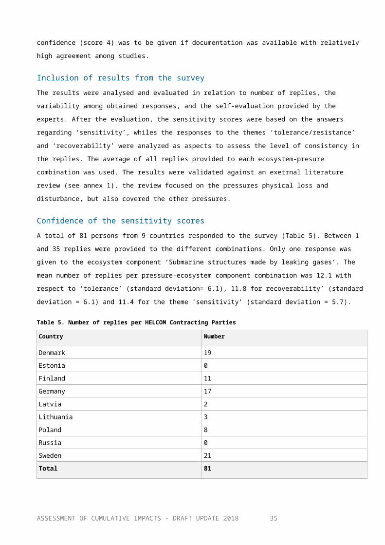
Figure 6. Ranking of pressures causing the cumulative impacts at regional scale (left panel) and list of most widely impacted ecosystem components (species or habitats; right panel). Note that only results for the twenty most impacted ecosystem components are shown. The ‘sum value’ for pressures is calculated as the sum of impacts from each pressure on all studied ecosystem components at Baltic Sea scale. For ecosystem components it is calculated as the sum of impacts from all pressures on each ecosystem component.[updated results, not final laytout]

Figure 6b. [option] Ranking of pressures causing the cumulative impacts at regional scale, when further aggregated into six main thesmes.[updated results, not final laytout]


4.3 CUMULATIVE IMPACTS ON BENTHIC HABITATSA separate analysis was carried out for potential cumulative impacts on the benthic habitats only, as these are particularly affected by physical pressures. In this case the evaluation was based on pressure layers representing physical loss and physical disturbance to the seabed, combined with information on the distribution of eight broad benthic habitat types and five habitat-forming species6.

The evaluation suggests that benthic habitats are potentially impacted by loss and disturbance in all sub-basins of the Baltic Sea, but the highest estimates were found for coastal areas and in the southern Baltic Sea (Figure 7). The most impacted sub-basins were identified as the Great Belts, the Sound, and the Bay of Mecklenburg (Figure 8). As the shallow waters usually host more diverse habitats, the impacts also accumulate more in coastal areas.

The human activities behind the cumulative impacts on benthic habitats, according to this assessment, are bottom trawling, shipping and sediment dispersal caused by various construction and dredging activities and disposal of the dredged sediment.

6) 8 broad scale habitats (Circalittoral hard substrate, Circalittoral mixed substrate, Circalittoral mud, Circalittoral sand, Infralittoral hard substrate, Infralittoral mixed substrate, Infralittoral mud and Infralittoral sand) and 5 habitat forming species (Furcellaria lumbricalis, Zostera marina, Mytilus edulis, Fucus spp. and Charophytes)ASSESSMENT OF CUMULATIVE IMPACTS – DRAFT UPDATE 2018

36

Figure 7. Map of potential cumulative impacts on benthic habitats in the Baltic Sea. The cumulative impacts are calculated based on the method of the Baltic Sea Impact Index as the ‘sum of impact’, specifically for the two pressures ‘physical loss’ and ‘physical disturbance. Benthic habitats were represented by eight broad scale habitat types and five habitat forming species (Furcellaria lumbricalis, Zostera marina, Mytilus edulis, Fucus spp. and Charophytes). The cumulative impact has been estimated based on currently best available data, but spatial and temporal gaps may occur in underlying datasets. Areas in white in the map are not covered by any of the pressures associated with impact on the seabed [new]


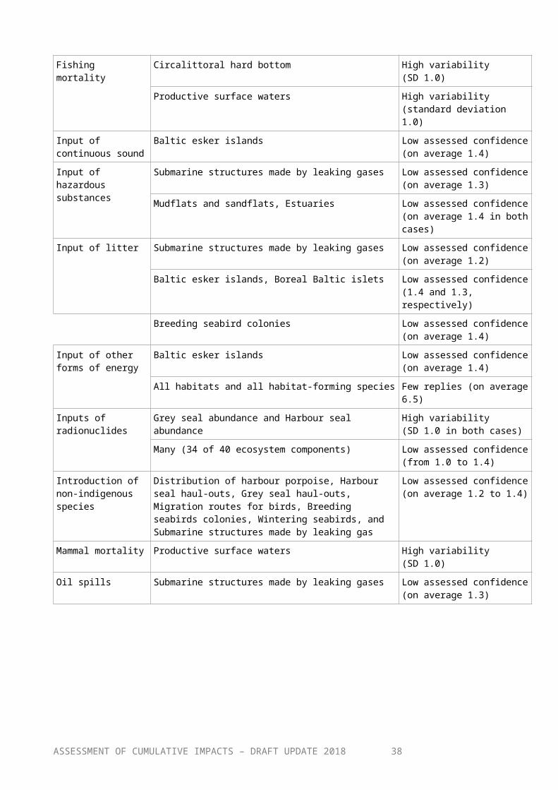
Northern Baltic ProperBothnian SeaBothnian Bay

Western Gotland BasinEastern Gotland Basin

The QuarkGulf of Finland

Gulf of RigaBornholm Basin

Gdansk BasinÅland Sea

Arkona BasinKattegatKiel Bay

Bay of MecklenburgThe SoundGreat Belt

0 0.1 0.2 0.3 0.4 0.5 0.6 0.7 0.8

Cumulative benthic impact per km²

Figure 8. Cumulative impacts on benthic habitats in the Baltic Sea sub-basins. The values are calculated as the ‘sum of impact’ from physical loss and physical disturbance on the studied benthic habitat types and habitat forming species, divided by the area of the sub-basin. The estimates are based on currently best available regional data, but spatial and temporal gaps may occur in underlying datasets.(updated)


4.4 PHYSICAL LOSS AND DISTURBANCE[Results same as in summary report chapter 4.7 to be added here, not updated yet]


4.5 CONFIDENCE IN THE ASSESSMENT[rewritten] The assessments of cumulative pressures and cumulative impacts, as well as the assessment of physical loss and disturbance, are highly dependent on the quality of the underlying data layers. The aim has been to collect and collate spatial information that is regional, so that the results will be comparable across areas. The data sets that were compiled provide a relatively comprehensive representation of prevailing pressures, species and habitats in the Baltic Sea.

Only in a few cases it was not possible to achieve data sets with sufficient spatial coverage for being included, namely regarding important habitats for flounder and migration routes for birds. Other originally planned data sets were not included in order to not double count impacts of aspects that were also represented in other layers, namely haulout areas for seals, and roach recruitement habitats. Among the pressures, effects of climate, which would potentially represented by changes in temperature and acidification, were not included for methodological reasons.

In some cases, data layers were still included despite some inconsistencies, in order to reflect the currently best available knowledge at regional scale. This concerns in particular pressure data layers on impulsive noise, dredging and fishing intensity, and ecosystem component layers on habitat-forming species.

Variation in the level of detail of individual data layers reduces the confidence in the assessment and the possibility to compared geographic areas with each other in more detail. While some underlying layers provide information on a relatively detailed spatial scale, other layers included in this assessment are not detailed enough to be relevant at a more local scale, for example many data sets showing species distributions and the data sets representing bird and seal hunting. Furthermore, some activities are represented by licenced areas, such as dredging, disposal of dredged matter and extraction of sand and gravel. These do not necessarily reflect the extent of the exerted pressure, as the activity may be undertaken only in parts of the licensed area.

There is some remaining uncertainty regarding the applied impact scores, as the number of replies for some combinations of pressures and ecosystem components was low in the expert survey, although the highest uncertainities were assiated with relatively rare ecosystem components at Baltic Sea scale, and hence potentially low influence on analyses, or distance combinations of ecosystem components and pressures (Table 6).

The focus of the assessment is to give a broad regional overview, whereas the level of accuracy in detailed results need to be evaluated on a case by case basis.


ReferencesAndersen, J.H. & A. Stock (Eds) Heinänen, S., M. Mannerla, & M. Vinther (2013): Human uses, pressures and impacts in the eastern North Sea. Aarhus University, DCE – Danish Centre for Environment and Energy. Technical Report from DCE – Danish Centre for Environment and Energy 18. 134 pp.

Andersson, M.H. (2011): Offshore wind farms – ecological effects of noise and habitat alteration on fish. Doctoral Dissertation. Department of Zoology, University of Stockholm.

Andrulewicz, E. D. Napierska & Z. Otremba (2003): The environmental effects of the installation and functioning of the submarine SwePol Link HVDC transmission line: a case study of the Polish Marine Area of the Baltic Sea. Journal of Sea Research 49: 337– 345.

Barrio Frojan, C.R.S., S.E. Boyd, K.M. Cooper, J.D, Eggleton & S. Ware (2008): Long-term benthic responses to sustained disturbance by aggregate extraction in an area off the east coast of the United Kingdom. Estuarine, Coastal and Shelf Science 79: 204-212.

Bergström, L., L. Kautsky, T. Malm, R. Rosenberg, M. Wahlberg, N. Åstrand Capetillo & D. Wilhelmsson (2014): Effects of offshore wind farms on marine wildlife—a generalized impact assessment. Environmental Reserach Letters9:1–12.

Bonsdorff, E. (1980): Macrozoobenthic recolonization of a dredged brackish-water bay in SW Finland. Ophelia, Supplement 1: 145-155.

Bonsdorff, E., E. Leppäkoski & C.S Österman (I986): Patterns in post-impact successions of zoobenthos following physical and chemical disturbance in the northern Baltic Sea. Publications of the Water Research Institute, National Board of Waters, Finland: 68.

Boyd S.E., H.L. Rees & C.A. Richardson (2000): Nematodes as sensitive indicators of change at dredged material disposal sites. Estuarine, Coastal and Shelf Science 51(6):805-819.

Boyd, S.E., D.S. Limpenny, H.L. Rees, K.M. Cooper & S. Campbell (2003): Preliminary observations of the effects of dredging intensity on the re-colonisation of dredged sediments off the southeast coast of England (Area 222). Estuarine, Coastal and Shelf Science 57 (1-2): 209–223.

Dalfsen van, J.A. & K. Essink (2001): Benthic community response to sand dredging and shoreface nourishment in Dutch coastal waters. Senckenbergiana maritima 31: 329-332.

Degerman, E. & R. Rosenberg (1981): Miljöeffekter av småbåtshamnar och småbåtar. SNV, PM 1399. 122 pp.

Eastwood, P. D., Mills, C. M., Aldridge, J. N., Houghton, C. A., and Rogers, S. I. (2007): Human activities in UK offshore waters: an assessment of direct, physical pressure on the seabed. – ICES Journal of Marine Science 64: 453–463.ASSESSMENT OF CUMULATIVE IMPACTS – DRAFT UPDATE 2018

41

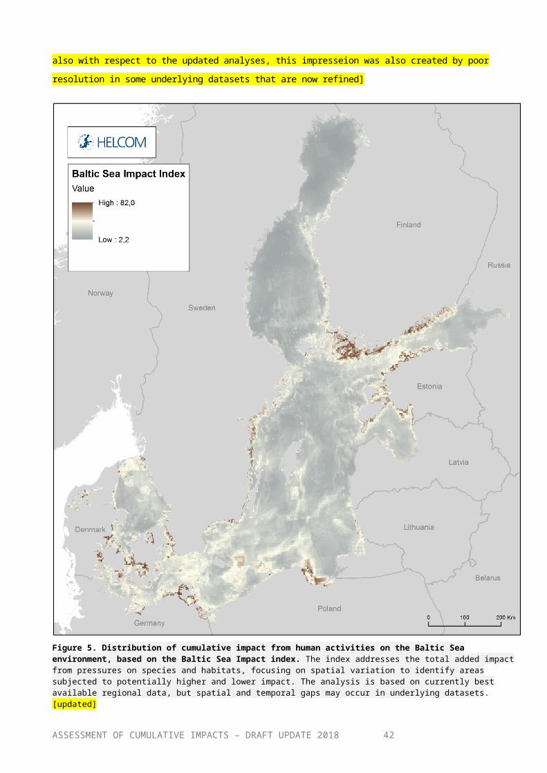
EC (2017a): Commission Decision (EU) 2017/848 of 17 May 2017 laying down criteria and methodological standards on good environmental status of marine waters and specifications and standardised methods for monitoring and assessment, and repealing Decision 2010/477/EU

EC (2017b): Commission Directive (EU) 2017/845 of 17 May 2017 amending Directive 2008/56/EC of the European Parliament and of the Council as regards the indicative lists of elements to be taken into account for the preparation of marine strategies.

Erftemeijer, P.L.A. & R.R.L. Lewis III (2006): Environmental impacts of dredging on seagrasses: A review. Marine Pollution Bulletin 52:1553-1512.

Eriksson B.K., A. Sandström, M. Isaeus, H. Schreiber & P. Karås (2004): Effects of boating activities on aquatic vegetation in the Stockholm archipelago, Baltic Sea. Estuarine, Coastal and Shelf Science 61:339–349.

Essink, K. (1999): Ecological effects of dumping of dredged sediments; options for management. Journal of Coastal Conservation 5: 69-80.

Gill, A.B. (2005): Offshore renewable energy: ecological implications of generating electricity in the coastal zone. Journal of Applied Ecology 42:605–615.

Halpern, B., S., S. Walbridge, K. A. Selkoe, C. V. Kappel, F. Micheli, C. D'Agrosa, J. F. Bruno, K. S. Casey, C. Ebert, H. E. Fox, R. Fujita, D. Heinemann, H. S. Lenihan, E. M. P. Madin, M. T. Perry, E. R. Selig, M. Spalding, R. Steneck & R. Watson (2008): A Global Map of Human Impact on Marine Ecosystems. Science 319:948-952.

Halpern, B., S, C. V. Kappel, K. A. Selkoe, F. Micheli, C. Ebert, C. Kontgis, C. M. Crain, R. G. Martone, C. Shearer, S. J. Teck (2009): Mapping cumulative human impacts to California Current marine ecosystems. Conservation letters 2: 138–148.

HELCOM (2010a): Ecosystem Health of the Baltic Sea 2003-2007. HELCOM Initial Holistic Assessment. Baltic Sea Environment Proceedings 122.

HELCOM (2010b): Towards a tool for quantifying anthropogenic pressures and potential impacts on the Baltic Sea marine environment. Baltic Sea Environment Proceedings 125.

HELCOM (2018): ‘State of the Baltic Sea’ report. XXX

HELCOM (2018b): HELCOM maps and data service. Available at: http://maps.helcom.fi/

HELCOM (2018c): HELCOM metadata catalogue. Available at: http://metadata.helcom.fi/

Ilus, E., J. Ojala & K.-L Sjöblom (1986): Effect of discharges from the Olkiluoto nuclear power station on the receiving waters. Publications of the Water Research Institute, National Board of Waters, Finland: 68.


http://metadata.helcom.fi/

http://maps.helcom.fi/

Karppinen, P., A. Haikonen & S. Vatanen (2011): Helsingin Energian Salmisaaren voimalaitosten jäähdytysvesien leviämiskartoitus. Kala- ja vesimonisteita: 66

Karppinen, P. & S. Vatanen (2013): Helsingin Energian Hanasaaren voimalaitoksen ja Katri Valan lämpö- ja jäähdytyslaitoksen jäähdytysvesien leviämiskartoitus. Kala- ja vesimonisteita: 95

Korpinen, S., L. Meski, J.H. Andersen, J.H. & M. Laamanen (2012): Human pressures and their potential impact on the Baltic Sea ecosystem. Ecological Indicators 15:105-114.

Knights, A., R.S. Koss, & L. Robinson (2013): Identifying common pressure pathways from a complex network of human activities to support ecosystem-based management. Ecological Applications 23: 755-765.

Kogan, I., C.K. Paull, L.A. Kuhnz, E.J. Burton, S. von Thun, H.G. Greene & J.P Barry (2006): ATOC/Pioneer Seamount cable after 8 years on the seafloor: Observations, environmental impact. Continental Shelf Research 26: 771–787

Korpinen, S., U.L. Zweifel, F. Bastardie, D. van Denderen, K. Hopp, P. Jonsson, P. Kauppila, M. Milardi , R. Nielsen, H. Nilsson, K. Norén, H. Nygård, M. Sköld, S. Valanko & M. Zettler(2017): Estimating physical disturbance on seabed. WP 3.1 Deliverable 1 of the BalticBOOST project.

Köster, F.W., B. Huwer, H.H. Hinrichsen, V. Neumann, A. Makarchouk, M. Eero, B.V. Dewitz, K. Hüssy, J. Tomkiewicz, P. Margonski, A. Temming, J.P. Hermann, D. Oesterwind, J. Dierking, P. Kotterba & M. Plikshs (2017): Eastern Baltic cod recruitment revisited—dynamics and impacting factors. ICES Journal of Marine Science 74:3-19.

Kotta, J., K. Herkul, I. Kotta, H. Orav-Kotta, & R. Aps (2009): Response of benthic invertebrate communities to the large-scale dredging of Muuga Port. Estonian Journal of Ecology 58: 286–296.

Kuhns, L.A. & M.B. Berg (1999): Benthic invertebrate community responses to round goby (Neogobius melanostomus) and zebra mussel (Dreissena polymorpha) invasion in southern Lake Michigan. Journal of Great Lakes Research 25: 910–917.

Lasalle, M.W. (1990): Physical and chemical alterations associated with dredging: an overview. In: Simenstad, C.A. (Ed). Effects of dredging on anadromous pacific coast fishes. Workshop Proceedings, Washington Sea Grant, Seattle, WA, USA. 1–12.

Lederer, A.M., J. Janssen, T. Reed & A. Wolf (2008): Impacts of the introduced round goby (Apollonia melanostoma) on dreissenids (Dreissena polymorpha and Dreissena bugensis) and on macroinvertebrate community between 2003 and 2006 in the littoral zone of Green Bay, Lake Michigan. Journal of Great Lakes Research 34: 690–697.

Leskinen, E., O. Kolehmainen. & I. Isotalo (1986): The response of periphytic organisms to the load of organic and inorganic nutrients from a fish farm. Publications of the Water Research Institute, National Board of Waters, Finland: 68.ASSESSMENT OF CUMULATIVE IMPACTS – DRAFT UPDATE 2018

43

Manso, F, R. Radzevicius, N. Blažauskas, A. Ballay & K. Schwarzer K (2010): Nearshore dredging in the Baltic Sea: Condition after cessation of activities and assessment of regeneration. Journal of Coastal Research 51: 187-194

Martin, D., F. Bertasi, M.A. Colangelo, M. de Vries, M. Frost, S. J. Hawkins, E. Macpherson, P.S. Moschella, M. P. Satta, R.C. Thompson & V.U. Ceccherell (2005): Ecological impact of coastal defence structures on sediment and mobile fauna: Evaluating and forecasting consequences of unavoidable modifications of native habitats. Coastal Engineering 52: 10-11.

Micheli, F., B. S. Halpern, S. Walbridge, S. Ciriaco, F. Ferretti, S. Fraschetti, R. Lewison, L. Nykjaer, & A.A. Rosenberg (2013): Cumulative Human Impacts on Mediterranean and Black Sea Marine Ecosystems: Assessing Current Pressures and Opportunities. PLoS ONE 8:e79889

Morton, B. (1996): The subsidiary impacts of dredging (and trawling) on a subtidal benthic Molluscan community in the Southern Waters of Hong Kong. Marine Pollution Bulletin 32: 701-10.

Munsterhjelm, R. (2005): Natural succession and human-induced changes in the soft-bottom macrovegetation of shallow brackish bays on the southern coast of Finland. Doctoral Thesis, University of Helsinki. Walter and Andrée de Nottbeck Foundation Scientific Reports: 26.

Newell, R.C., L.J. Seiderer & D.R. Hitchcock (1998): The impact of dredging works in coastal waters: a review of the sensitivity to disturbance and subsequent recovery of biological resources on the seabed. Oceanography and Marine Biology: an Annual Review, 36: 127–178.

Nichols, M., R.J. DiazJ. & L.C Schaffner (1990): Effects of hopper dredging and sediment dispersion, chesapeake bay. Environmental Geology and Water Science Journal 15. DOI: 10.1007/BF01704879

Orviku, K., H. Tõnisson, R. Aps, J, Kotta, I, Kotta, G. Martin, Ü. Suursaar, R. Tamsalu & V. Zalesny (2008): Environmental impact of port construction: Port of Sillamäe case study (Gulf of Finland, Baltic Sea). In: 2008 IEEE/OES US/EU-Baltic International Symposium: US/EU-Baltic International Symposium ‘Ocean observations, ecosystem-based management & forecasting’; Tallinn 27-29 May, 2008. IEEE-Inst Electrical Electronics Engineers Inc. 2008:350-359.

Oulasvirta P. & J. Leinikki (2003): Veneilyn ympäristövaikutukset luonnonsatamissa. Suomen ympäristö 605. 91 pp.

Phua, C., S. van den Akker, M. Baretta M & J. van Dalfsen (2004): Ecological Effects of Sand Extraction in the North Sea. The North Sea Foundation, 22 pp.

Powilleit, M., G. Graf, J. Kleine, R. Riethmüller, K. Stockmann, M.A. Wetzel & J.H.E. Koop (2009): Experiments on the survival of six brackish macro-invertebrates from the Baltic Sea after dredged spoil coverage and its implications for the field. Journal of Marine Systems 75:441–451.

Roth, E.M., L.A. Verhoef & M.W.L. Dingenouts (2004): Overview of Environmental Impacts of Offshore Wind energy. ASSESSMENT OF CUMULATIVE IMPACTS – DRAFT UPDATE 2018

44

Rytkönen, J., T. Kohonen & J. Virtasalo (2001): Laivaliikenteen aiheuttama eroosio Pohjois-Airistolla (Erosion caused by ship traffic in the northern archipelago of Airisto – In Finnish). Vesitalous 30: 30-36.

Sahla, M. (2015): Sensitivity and the gaps of knowledge for cumulative human pressure modelling in the Archipelago Sea. [Summary in English] M.Sc. Thesis, University of Turku, Faculty of Mathematics and Natural Sciences, Department of Geography and Geology. 95 pp.

Sandström, A., B.K. Eriksson, P. Karås, M. Isæus & H. Schreiber (2005): Boating and navigation activities influence the recruitment of fish in a Baltic Sea archipelago area. Ambio 34: 125-130.

Soomere T & J. Kask (2003): A specific impact of waves of fast ferries on sediment transport processes in Tallinn Bay. Proceedings of the Estonian Academy of Sciences: Biology and Ecology 52:319–331

Stock, A. (2016): Open Source Software for Mapping Human Impacts on Marine Ecosystems with an Additive Model. Journal of Open Research Software, 4: e21. DOI: http://dx.doi.org/10.5334/jors.88

Syväranta, J. & J. Leinikki (2014): Taulukarin läjitysalueeseen liittyvät silakan kutuselvitykset (In Finnish). Alleco Oy raportti 2014:1.

Syväranta, J. & P. Vahteri (2013): Turun sataman kalatalousvaikutusten tarkkailututkimukset 2012 (In Finnish( Alleco Oy raportti 2013:1.

Syväranta, J. & Leinikki, J. (2015): Taulukarin kasvillisuus- ja sedimenttitutkimukset 2014 (Investigations of the vegetation and sediments of Taulukari – in Finnish) Alleco Oy raportti 2015: 1.

Syväranta, J., J. Leinikki & J. Leppänen (2013): Taulukarin– Mustakuvun kasvillisuus- ja sedimenttitutkimukset 2012 (In Finnish). Alleco Oy raportti 2013: 3.

Tillin, H.M., S.C. Hull & H.Tyler-Walters (2010): Development of a Sensitivity Matrix (pressures-MCZ/MPA features). Report to the Department of Environment, Food and Rural Affairs from ABPMer, Southampton and the Marine Life Information Network (MarLIN) Plymouth: Marine Biological Association of the UK. Defra Contract No. MB0102,Task 3A: 22.

Torn, K., G. Martin, J. Kotta & M. Kupp (2010): Effects of different types of mechanical disturbances on a charophyte dominated macrophyte community. Estuarine, Coastal and Shelf Science 87:27–32.

Vahteri, P. & I. Vuorinen (2001) Silakan lisääntyminen vaarassa Pohjois-Airistola (In Finnish). Vesitalous 3: 37-38.

van der Wal, J.T. & J.E. Tamis (2014): Comparing methods to approach cumulative effects in the North-East Atlantic: CUMULEO case study. IMARES - Institute for Marine Resources & Ecosystem Studies C178/13.


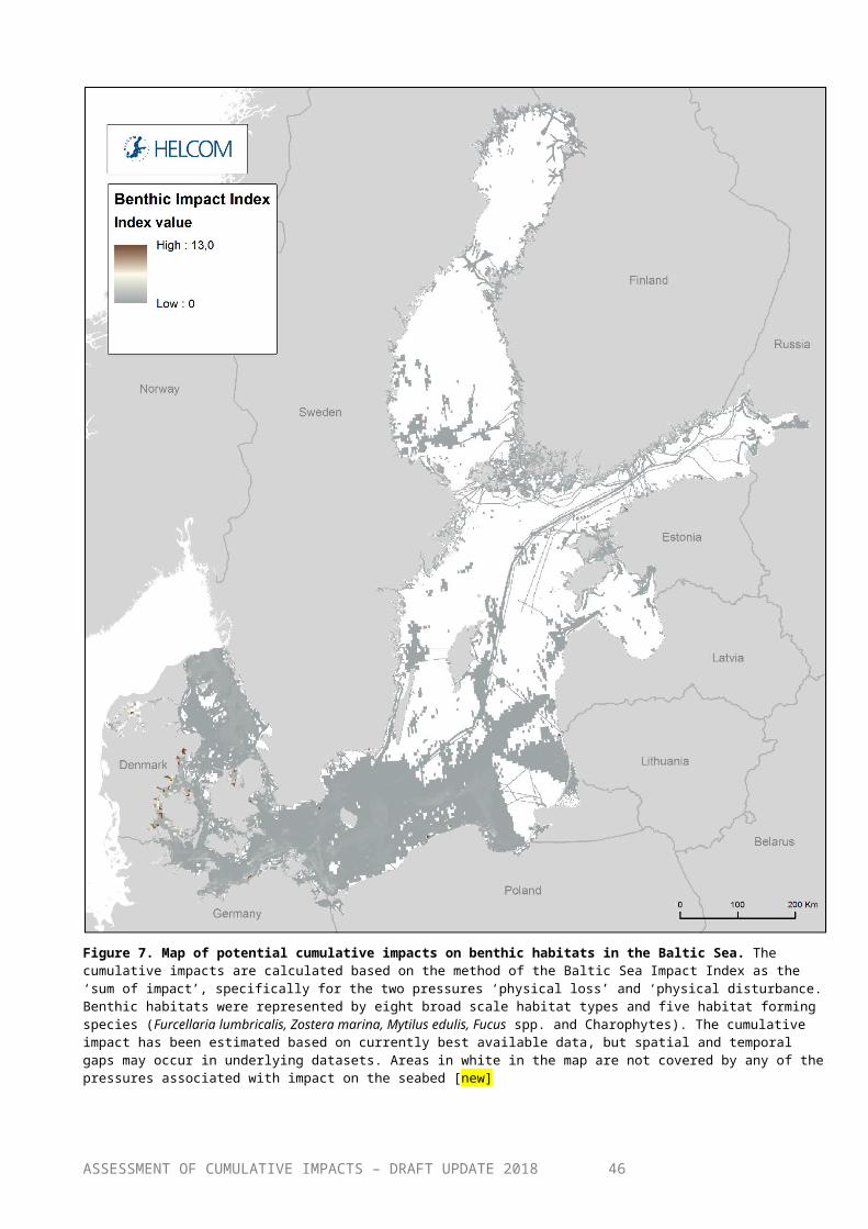
Vatanen S, A. Haikonen & J. Kervinen (2014): Uudenkaupungin väylän ja sataman ruoppaus- ja läjityshankkeen vesistö- ja kalataloustarkkailu – Ennakkotarkkailu sekä rakentamisen aikainen tarkkailu vuonna 2013 (In Finnish). Kala- ja vesimonisteita 137.

Vatanen, S., A. Haikonen & J. Kervinen (2015): Uudenkaupungin väylän ja sataman ruoppaus- ja läjityshankkeen vesistö- ja kalataloustarkkailu – Rakentamisen aikainen tarkkailu vuonna 2014 (Survey of the effects on water and fisheries of ongoing dredging and dumping activities in the Uusikaupinki waterway and harbour 2014 – In Finnish). Kala- ja vesimonisteita 170.

Vatanen S, A. Haikonen & A. Piispanen (2012): Vuosaaren sataman rakentamisen aikaisen (2003-2008) vesistö- ja kalataloustarkkailun yhteenvetoraportti. Kala- ja vesimonisteita:57.

Vatanen, S., A. Lindfors & M. Laamanen (2010): Naantalin alueen vuoden 2009 vesistötöiden vesistö- ja kalatalousseurannan loppuraportti (Final report from the survey of effects of underwater activities on water and fisheries in Naantali 2009– In Finnish). Kala- ja vesimonisteita 36.

Wan Hussin, W.M.R., K.M. Cooper, C.R.S. Barrio Frojan, D.C. Defew & D.M. Paterson (2012): Impacts of physical disturbance on the recovery of a macrofaunal community: A comparative analysis using traditional and novel approaches. Ecological Indicators 12: 37-45.

Wilhelmsson, D., T. Malm, R. Thompson, J. Tchou, G. Sarantakos, N. McCormick, S. Luitjens, M. Gullström, J.K. Patterson Edwards, O. Amir, O. & A. Dubi (Eds.) (2010): Greening Blue Energy: Identifying and managing the biodiversity risks and opportunities of offshore renewable energy. Gland, Switzerland: IUCN. ISBN: 978-2-8317-1241. 102pp.


Annex 1. Detailed description of the input data for the aggregated pressure layers

The table below gives more details to how the aggregated pressure layers included in the Baltic Sea Impact Index and the Baltic Sea Pressure Index were compiled. The table columns give: A: the identity of the aggregated pressure layer (APL); B: its temporal nature, indicating whether it represents a cumulative pressure (CUM; values over the assessment period are summed) or a temporary pressure (TEMP; average values over the assessment years are used); C : underlying spatial data sets included; D: the spatial extent applied; E: justification for spatial extent; F: data processing applid to arrive at common unit, and final metric; G: Whether down-weighting by seabed exposure and water depth was applied, and H: method for aggregating spatial data sets to one aggreatred pressure layer. *With respect to physical loss and disturbance it should be noted that whether an activity in reality leads to loss of or disturbance of the seabed depends on many factors, such as the diration and intensity of the activity, the technique used and the sensitivity of the area affected. The identification of which activities lead to loss and/or physical disturbance is still under development

A.Pressurelayer

B.Nature

C. Underlying spatial datasets

D. Spatial extent

E.Reference

F. Data and data processing

G. Depth / exposure weighting

H.Aggregation method

Physical loss (permanent effects on the seabed)*

Cum Land claim Area of polygon or 50 m buffer for points, 30m buffer for lines

Estimated based on wind turbine erosion protection (van der Wal & Tamis 2014). No direct reference.

Calculate lost area. In a grid cell: calculate proportion of the cell area.

Not relevant

Activities are combined and potentially overlapping areas are removed. Dataset is clipped with coastline. Combined layer is intersected with 1 km grid to calculate % of area lost within a cell.

Watercourse modification

50 m buffer as above.


Not relevant

Coastal defence and flood protection

50 m buffer for lines, area of polygon

as above


Not relevant


A.Pressurelayer

B.Nature


D. Spatial extent

E.Reference




Extraction of sand and gravel

Area of polygon - Calculate lost area. In a grid cell: calculate proportion of the cell area.

Exposure affects recovery, but this is not included

Dredging (capital) Area of polygon or a 25/50 m buffer for <5000 m3 / >5000m3 sites

- Calculate lost area (polygon/buffer)

Exposure affects recovery, but this is not included

Oil platforms 25 m buffer As above.


Not relevant

Pipelines 15 m buffer Between cables and wind farms


Not relevant

Wind turbines (operational)

30 m buffer around each turbine

van der Wal & Tamis 2014


Not relevant

Cables 1.5 m buffer Estimate based on side-scan sonar photos (BalticBOOST case study in Mecklenburg Bight)


Not relevant

Harbours Polygon with 200 m buffer

Orviku et al. 2008; and as for ‘Maintenance dredging’


Not relevant

Marinas and leisure harbours

Point with 200 m buffer

Eriksson et al. 2004, Sandström et al. 2005


Not relevant


A.Pressurelayer

B.Nature


D. Spatial extent

E.Reference




Bridges 2 m buffer TAPAS project: based on erosion protection


Not relevant

Oil terminals, refineries

Point with 200 m buffer

Based on harbours (Orviku et al. 2008)


Not relevant

Finfish mariculture 150 m buffer Leskinen et al. 1986


Not relevant

Shellfish mariculture

Area of polygon, 150 meter buffer for points

- Calculate lost area. In a grid cell: calculate proportion of the cell area.

Not relevant

Shipping density AIS data calculated directly to 1 km grid cells. No spatial impact outside grid cells.

See Table A.2.2

Average of total shipping density in a 1km x 1 km cell 2011-2014, log-transformed, normalized.

rescaled with depth: 0-10 m= 100%10-15 m= 50%15-20 m= 25%20-25 m= 10%25m < =0%

Physical disturbance or damage to seabed (temporary or reversible effects)*

Temp.

Recreational boating and sports

Total fuel consumption of recreational boats modelled directly to 1 km grid cells. No spatial impact outside grid cells.

See also Table A.2.2

Total fuel consumption of leisure boats modelled in SHEBA project. Fuel usage range in a 1km x 1 km cell in 2014, log-transformed, normalized.

Rescaled with depth: 0-2m= 100%2,1-3 m= 75%3,1-4 m= 50%4.1-5 m= 25%5m < =0%

Spatial extents, including spatial attenuation of the pressures, are calculated per specific data sets. Mean


A.Pressurelayer

B.Nature


D. Spatial extent

E.Reference




pressure intensity per grid cell is assigned to the grid cell. The final grid cell intensity is downweighted (by areal %) if the pressure area is smaller than the grid cell. Activities are weighted according to the method described in the document. All the pressure intensities of specific pressure layers are summed per grid cell.

Extraction of sand and gravel

3 km buffer with sharp decline after 0.5 km (type D decline)

See Table A.2.1 for type and A.2.4 for extent

Average amount of extracted material over years, if value missing, 25% percentile of the existing information is given, normalized

Weighted by the exposure map

Dredging (maintenance)

500 m buffer with sharp decline (type D decline). Converted first to 100 m2 and then to 1 km2 grid cells.


Average amount of dredged material over years, if value missing 25% percentile of the existing information is given, normalized


Deposit of dredged material

500 m buffer with sharp decline (type D decline).


Average amount of deposited material 2011-2014, if value missing 25% percentile of the existing information is given, normalized


Wind farms (under construction)

1 km buffer with sharp decline after 0.5 km for wind turbines under construction.



Wind farms (operational)

0.1 km buffer with sharp decline.


Not relevant

Cables (under construction)

1 km buffer with sharp decline after 0.5 km for cables under construction.


Presence of constructed cables, intensity scaled by their area in the grid cell



A.Pressurelayer

B.Nature


D. Spatial extent

E.Reference




Pipelines (operational)

0.3 km buffer with linear decline.

Based on the operational wind farms (see Table A.2.2)

Presence of operational pipelines, intensity scales by their area in the grid cell

Fishing intensity (subsurface swept area ratio average 2011-2013)

0.05 x 0.05 c-square degree grid (reporting unit for VMS data from ICES)

- Average subsurface swept area ratio average 2011-2016, converted to 1x1km raster grid

Not relevant

Coastal defence and flood protection (under construction)

500 m buffer with sharp decline.

See Tables A.2.1-2 based on wind farms and cables.

Area of coastal defence and flood protection under construction.


Finfish mariculture 1 km buffer linear decline

Based on ‘Disposal of dredged material’.

Average P load 2011-2015, if values missing 25% percentile was given, normalized


Shellfish mariculture

area of polygon Based on ‘Disposal of dredged material’.

Average production in 2011-2015, if values missing, 25% percentile was given, normalized


Furcellaria harvesting

No buffer considered

- Calculated amount/area of harvested material, normalized

Not relevant

Scallop and blue mussel dredging

No buffer considered,

- Sum of scallop and blue mussel dredged per year, averaged for 2011-2015, normalized

Not relevant


A.Pressurelayer

B.Nature


D. Spatial extent

E.Reference




Changes to hydrological conditions (e.g. by constructions impeding water movements)

Cum.

Water course modification

1 km buffer Extent based on wind farms and cables, but expanded to 1 km because hydrological parameters are widely spreading.

Location of water course modifications

Not relevant

Spatial extents and potential attenuation gradients are assigned to the specific pressure layers. They are merged (by affected area, km2) to avoid overlapping areas. Intersected with 1 km grid to calculate % of area affected within a cell.

Wind turbines (operational)

300 m buffer around each turbine with linear decline

See Table A.2.1.

Location of operational wind turbines as points

Not relevant

Oil platforms 500 m buffer around each turbine with linear decline

See Table A.2.1.

Location of oil platforms as points

Not relevant

Hydropower dams a grid cell in the estuary (no extent added)

- locations of hydropower dams - those that are operational and produces energy

Not relevant

Inputs of continuous anthropogenic sounds (into water)

Temp.

Ambient underwater noise

BIAS project ambient underwater noise 2014, data modelled into 0.5 km x 0.5 km grid.

- Ambient underwater sound pressure level at 1/3 octave bands 125 Hz exceeding noise levels 5% of the time in the full water column, normalized.

Not relevant

Data normalized by setting 92 and 127 db re1uPa as pressure thresholds for 0 and 1 respectively


A.Pressurelayer

B.Nature


D. Spatial extent

E.Reference




Inputs of impulsive anthropogenic sound (into water)

Temp.

Impulsive noiseevents 2011-2016

Data converteddirectly to 1km gridcells

- Data from HELCOM-OSPARDatabase for impulsive noiseand national data call (polygons,points, lines) with noise valuescategorized from very low, low,medium, high and very high. Sum of all events calculated per 1x1 km grid cell. Normalized.

Not relevant

Sum of events based onnoise value codes.

Input of heat (e.g. by outfalls from power stations) into water

Temp.

Discharge of warm water from nuclear power plants

1 km buffer with steep decrease around outlet

See Table A.2.1 for type. Extent based on Ilus et al. 1986,

Average input of warm water (Celcius) from the nuclear power plant outlets

Not relevant

Not relevant

Fossil fuel energy production (only location available)

1 km buffer with steep decrease around outlet

See Table A.2.1 for type. Extent based on Karppinen et al. 2011, Karppinen & Vatanen 2013

Average input of warm water (Celcius) from the nuclear power plant outlets

Not relevant

Sum of the input of warm water.


A.Pressurelayer

B.Nature


D. Spatial extent

E.Reference





CHASE Assessment tool concentration component: mean contamination ratio per assessment station.

Interpolated map from the CHASE station data.

- Mean contamination ratio of the CHASE assessment tool concentration component. Values classified according to classification presented at the supplementary report for hazardous substances. Classified values interpolated, generalized and normalized.

Not relevant

Introduction of radionuclides

Temp.

10 km buffer with linear decline from discharges of radioactive substances

Gradual buffer around outlet to 10 km distance

Based on Ilus et al. 1986

Annual averages of CO60, CS137 and SR90 from the period 2011-2015 per nuclear power plant. Aggregation to be agreed intersessionally between HELCOM Mors Expert group and the Secretariat.

Not relevant

Not relevant


A.Pressurelayer

B.Nature


D. Spatial extent

E.Reference




Oil slicks and spills

Temp.

Oil slicks and spills from ships and oil platforms

Buffer area depending on reported spill area

See next column.

If oil spill volume was missing (67/560), median of the rest was given. If area of spill was missing (103/560), mean of the existing was given. If the spill was < 1km2, the value of spill volume was given directly to 1km2 grid cell. If the spill area > 1km2, the estimated volume of the spill was divided by the spill area to get the estimated amount of oil / km2. This value was given to the entire spill area.

Not relevant

Not relevant

Temp.

Polluting ship accidents

Point, converted directly to 1 x 1 km grid

See next column.

9/24 accidents with oil spills were missing spilled oil volume, thus a mean of reported volumes was given to accidents with missing oil volume. Spill volume in m3 was converted to grid

Not relevant

sum of spill volume


A.Pressurelayer

B.Nature


D. Spatial extent

E.Reference




Relative distribution of nutrient concentration (phosphorus and nitrogen)

Interpolated nitrogen and phosphorus concentrations in separate layers

Values are aggregated to 5x5km grid and annual seasonal averages calculated.

- Total nitrogen and total phosphorus concentrations (annual seasonal averages) from 0-10m surface layer for 2011-2016. Lowest and highest 5 percentile of values grouped together to avoid overestimation of extreme values. Generalized, log-transformed and normalized.

Not relevant

Not relevant (separate data layers)

Disturbance of species due to human presence

Temp.

Recreational boating and sports

Total fuel consumption of recreational boats modelled directly to 1 km grid cells.

- Total fuel consumption of recreational boats presented as presence / absence. Rescaled with depth, log-transformed and normalized.

Rescaled with depth: 0-10m= 100%10-15 m= 70%15-20 m= 50%20-30 m= 20%30-40 m = 10%45m < =0%

Temp.

1 km buffer. Bathing sites, beaches

Point data converted directly to 1 km grid cells

Estimate by TAPAS project of the human disturbance (noise, water sports, visual disturbance)

Location of beaches presented as presence / absence

Not relevant

Specific pressure layers first modified by spatial extents and depth influence. Each of them is considered as of equal importance (same weight). Calculate the sum of the pressure


A.Pressurelayer

B.Nature


D. Spatial extent

E.Reference




in a cell.Urban land use Urban land use data was first converted to 1 km grid cells and expanded with 1 km.

Estimate of the human disturbance (noise, visual disturbance)

Urban land use data was first converted to 1 km grid cells and expanded with 1 km. Thus, coastal urban areas extended also to the sea. These areas were given value 1 and other sea areas, value 0.

Not relevant

Extraction of, or mortality/injury to fish

Temp.

0 km. Extraction of fish species by recreational fishery.

Reported per country for eel, cod and salmon (tonnes).

- Extraction of fish species by recreational fishing, average of 2011-2016. For cod, recreational landings (tonnes/km2) were added to commercial catches.

Not relevant

Tonnes/km2 values for cod, summed with tonnes/km2 values from commercial catches. Log transformed.

0 km. Extraction of target fish species (cod, herring, sprat) in commercial fishery

Reported per ICES Rectangles, covers the whole Baltic Sea. Values are redistributed with fishing effort data c-squares (all gears) 2011-2013. Effort values missing from Russia and sub basin average values given.

- Extraction of fish species (landings) per ICES c-squares, average of 2011-2016. Landings calculated per km2.

Not relevant

Log transformed. For cod, recreational fisheries catches were added (see below).


A.Pressurelayer

B.Nature


D. Spatial extent

E.Reference




Extraction of, or mortality/injury to seabirds (e.g. hunting, predator control)

0 km. Game hunting of seabirds

Varying reporting units, from counties to HELCOM subdivisions, seaward boundary 3nm from coastline including islands and skerries.

- Species summed together, average of killed seabirds of years 2011-2015 per reporting unit, numbers of killed birds / km2 calculated and generalized for the whole reporting unit, normalized

Not relevant

Temp.

0 km. Predator control of seabirds

Varying reporting units, from counties to HELCOM subdivisions, seaward boundary 3nm from coastline including islands and skerries.

- Total number of killed cormorants per year averaged for 2011-2015, numbers of killed birds / km2 calculated and generalized for the whole reporting unit, normalized

Not relevant

Normalized values summed together

Extraction of, or mortality/injury to mammals

0 km. Hunting of seals

Varying reporting units, from counties to HELCOM subdivisions

- Total number of killed seals (per species) averaged for 2011-2014, numbers of killed seals/ km2 calculated, and generalized for the whole reporting unit, normalized

Not relevant

Not relevant (as the species are presented separately in the ecosystem components)

Introduction of non-indigenous species and translocations

Temp.

50 km buffer. Spread of non-indigenous species

Reported per coastal areas

- Number of NIS per HELCOM sub-basins and coastal areas, generalized for the whole reporting unit.

Not relevant

Not relevant


Annex 2. Details on expert survey and literature review to set the sensitivity scoresThe sensitivity score were developed with the EU co-funded TAPAS project and were identified based on a detailed questionnaire to be responded by Baltic Sea experts through the HELCOM contact points. The replies provide the basis for setting sensitivity scores for use in the Balctic Sea Impact Index as presented in Chapter 3 of this report, and partially supported the development of aggregated pressure layes as described in Chapter2.

The replies from the expert survey were validated against a literature review conducted with the EU co-funded BalticBOOST project (Tables A.2.3-7).

Description of the expert survey This expert survey was developed in Microsoft Exce together with a guidance document. In addition, the expert survey included guidance text in several steps and also comments for specific points7.

The survey covered a matrix of 750 potential pressure- and ecosystem-specific combinations (See tables 1, 3 and 4 in this report). In order to estimate as robust pressure- and ecosystem component specific sensitivity scores as possible, the questionnaire addressed the following 6 themes: (1) Tolerance/resistance, (2) Recoverability, (3) Sensitivity, (4) Impact distance, (5) Impact type and (6) Confidence.

For tolerance/resistance, participants in the survey had the following 3 options: High, Medium and Low (lethal). To support the participants, the survey included an explanatory text: “Tolerance (resistance): How tolerant or resistant is the ecosystem to the human pressure? For example, for a pressure that has devastating effects on the ecosystem component in question, you should set the tolerance to a low value. If you should think that a specific human pressure has a relatively minor effect on this ecosystem component, you should set the tolerance to high. Factors to take into account when making your judgment are the typical intensity/level of the pressure when it occurs in the sea and typical biological effects (e.g. the number of trophic levels affected). You should not take into account if there actually is a spatial overlap between the pressure and the ecosystem component, since this will be included in other parts of the assessment.”

For recoverability, the participants had the following 3 options: High, Medium and Low (> 10 years). To support the participants, the survey included an explanatory text: “Recoverability: Reflects how long it takes for the ecosystem component to recover once the pressure ceases). The recoverability is estimated on a scale from immediate (high) to >10 years (low). 7 Permanent storage address to be added. Currently at: http://www.helcom.fi/Documents/TAPAS_survey.xlsm.


http://www.helcom.fi/Documents/TAPAS_survey.xlsm

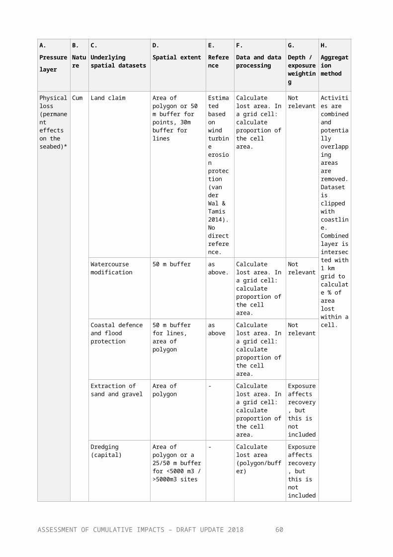
Some human activities cause pressures which cease immediately after stopping the activity (such as noise from shipping), while some pressures may stay in the environment for a long time (such as contaminants and nutrients from pollution). However, independent of these differences, recovery times of the ecosystem components may differ. For instance, impacts on the species may last longer than the actual time the pressure exists in the sea.”

For sensitivity, the participants had the following 3 options: High, Medium and Low. To support the participants, the survey included an explanatory text: “Sensitivity: Although tolerance and recoverability affect sensitivity, other factors may also have an influence, and in some cases the different components of overall sensitivity may not be well known. Sensitivity was asked for as a complement to the above questions to ensure confidence in how the impact scores are calculated. In general, when rating tolerance, recoverability and sensitivity in the survey, you should imagine the human pressures as they typically occur in the study area. For instance, when replying for fish farms, imagine a typical fish farm, neither extremely big nor small. For commercial shipping, you should think of a busy, but not extraordinarily busy, shipping route. Also, assume that the stressor and the ecosystem occur together in the same place. As an example, if you know that an ecosystem component does not naturally occur close to any existing shipping routes, this does not mean that you should give it low vulnerability values. Instead, rate its vulnerability for the (hypothetical) case that the stressor and the ecosystem do occur in the same place, and the stressor is occurring at a typical intensity and frequency.”

For impact distance, the participants were asked to answer the following question: “How far from the pressure/activity source will potential impacts on the ecosystem diminish to a negligible level, given its vulnerability?” The possible answers to this question were: (1) Local, (2) 1 km, (3) 5 km, (4) 10 km, (5) 20 km and (6) > 50 km.

For impact type, the participant were asked to identify which of the following ‘impact distance types’ (i.e. form of decay with increasing distance from the pressure source) in Figure A.2.1 could be assumed to be relevant for the pressure in question.

Figure A.2.1. Impact types A, B, C and D. Type A describes a pressure that has a similar impact at most of its distribution range and then rapidly drops, type B describes a pressure that declines monotonously in strength from the source, type C describes a pressure having a somewhat limited decline within a given distance followed by a sharp decline, while type D describes a pressures which mostly has an strong impact in its vicinity.


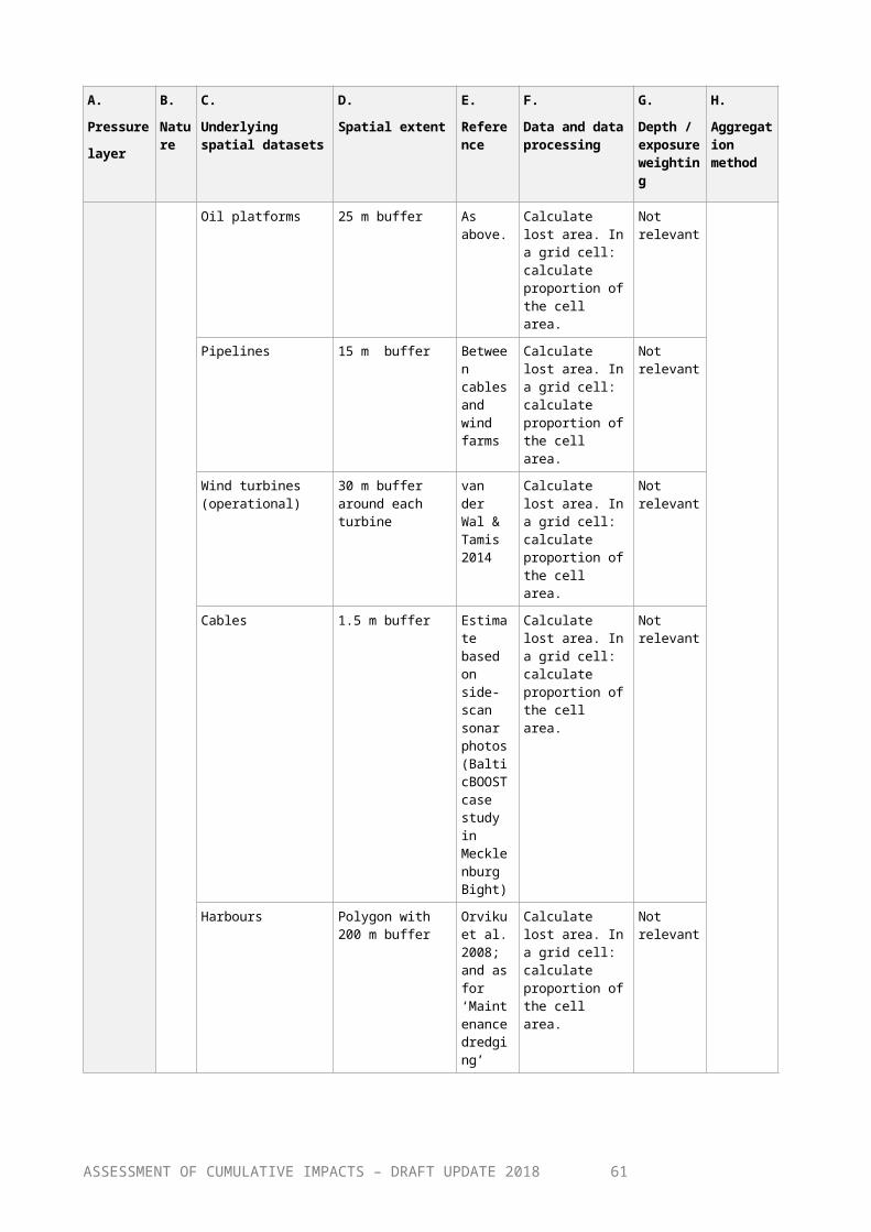
For confidence, participants were asked to self-evaluate the confidence of their judgment, reflecting the information on which their answers are based. For example: (1) a low confidence should be assigned if limited or no empirical documentation (e.g. judgement is based on inference from other, similar ecosystem components/pressure types or from knowledge on the physiology and ecology of the species etc.). (2) a moderate confidence should be assigned if documentation is available, but results of different studies may be contradictory (e.g. including also grey literature with limited scope), and (3) a high confidence should only be given if documentation is available and with relatively high agreement among studies.

Sensitivity scores from the expert surveyA summary of the results is shown presented in Table 4 of the main report.

Results for ‘Tolerance’ With regard to the theme 1 (tolerance), there was a large variation in the number of replies per combination of pressure and ecosystem component. Between 1 and 35 replies were provided to the different combinations (mean number of replies = 12.1, standard deviation= 6.1). Only one response was given to the ecosystem component ‘Submarine structures made by leaking gases’ (also with respect to themes 2 and 3 below). There was also some variability in the obtained responses, that is, the scores provided by different experts. The standard deviation around the mean for responses to a certain combination of pressure and ecosystem component was on average 0.55, ranging between 0 and 1. Replies with high variability (a standard deviation above 1.0) can be regarded7 as less reliable compared to those with lower standard deviation.

Results for ‘Recoverability’ For theme 2 (recoverability), there was also large variation in the number of replies for each combination of pressure and ecosystem component (between 1 and 35 replies, mean number of replies = 11.8, standard deviation = 6.1). The variability in scores among obtained responses was higher than for tolerance. The standard deviation around the mean for responses to a certain combination of pressure and ecosystem component was on average 0.62, ranging between 0 and 1.41.

Results for ‘Sensitivity’ For theme 3 (sensitivity) the number of replies for each combination of pressure and ecosystem component ranged between 1 and 35, with a mean value of 11.4 responses per combination (standard deviation = 5.7). The variability in scores among responses, as measured by the standard devaluation from the mean, was on average 0.62, ranging between 0 and 1.41.


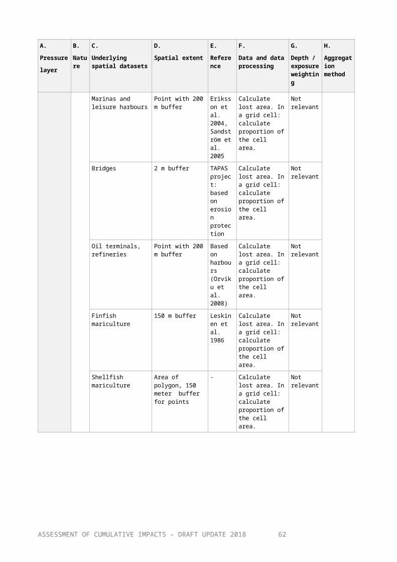
Correlation among results The correlation between the sensitivity scores and the other two themes (tolerance, recoverability) was evaluated as part of the quality assurance. The highest correlation was observed between ‘sensitivity- and ‘tolerance’ (Figure A.2.1). According to the definition of the factor ‘sensitivity’ in the expert survey, it should include the aspects of both of the other two factors.

Figure A.2.1. Correlation between the mean scores for ‘tolerance’ and ‘sensitivity’ among all responses for combinations of pressures and ecosystem component. The obtained correlation value R2 was 0.63, which is higher than for the correlations between scores for ‘sensitivity’ and ‘recoverability’ (R2=0.20).

Survey results regarding impact types and distancesTable A.2.1 shows the impact distances and impact types per pressure based on the results from the expert survey. The minimum, maximum and mean distances were first calculated based on all obtained responses at the level of each ecosystem component, and the table shows the corresponding values subsequently calculated across all ecosystem components. The standard deviation shows variability in the mean value among the ecosystem components.

Table A.2.2. shows the spatial extent of physical disturbance from different human activities based on literature. The extents were estimated as the distance from the activity at which the pressure intensity can be considered negligible to complement to the expert survey for processing the pressure data layers.


Table A.2..1. Impact distances and impact types per pressure, based on the results from the expert survey. The column ‘impact type’ shows what impact type was indicated in most cases among the respondents. The value is the average % of the replies indicating that pressure type across all ecosystem components (higher values indicate that the type was identified more frequently as the predominating type, as depicted in Figure A.1.1). For pressures marked *, the aggregated pressure layes were developed based on literature information instead. Pressures marked ** were not finally used in the assessment.

Pressure Min (km) Max (km)

Mean (km)

Standard deviation (km)

Impact type

1. Physical loss* 0.1 9.4 2.4 2.6 D (58%)2. Physical disturbance* 0.8 10.6 2.5 2.3 D (34%)3. Changes to hydrological conditions* 0.5 26.8 7.2 6.3 A (39%)4. Inputs of continuous anthropogenic 5.0 26.4 15.6 5.2 B (31%)5. Inputs of impulsive anthropogenic 2.5 25.7 11.8 5.2 N.A.6. Inputs of other form of energy (electromagnetic and seismic waves)

0.1 10.2 4.9 3.6 A (48%)

7. Input of heat 0.1 6.5 3.0 1.9 D (33%)8. Inputs of hazardous substances 0.5 32.9 20.2 7.5 D (39%)9. Inputs of nutrients 13.7 43.0 25.7 7.4 B (53%)10. Introduction of radionuclides 10.0 46.4 34.6 6.6 D (40%)11. Oil slicks and spills 7.1 33.2 16.5 6.1 D (38%)12. Inputs of litter 6.2 34.1 15.7 6.8 D (60%)13. Inputs of organic matter 9.3 36.9 20.5 7.4 B (52%)14. Disturbance of species due to 0.0 14.0 1.9 2.7 C (32%)15. Extraction of, or mortality/injury to 2.0 38.6 11.6 9.2 C (30%)16. Extraction of, or mortality/injury to mammals and seabirds (e.g. hunting, predator control)

1.0 42.5 19.7 10.5 B (42%)

17. Introduction of non-indigenous species and translocations

14.0 41.0 27.8 6.8 B (47%)

18. Changes in climatic conditions** 22.0 50.0 46.9 7.1 A (28%)19. Acidification** 32.0 50.0 46.1 5.3 A (40%)


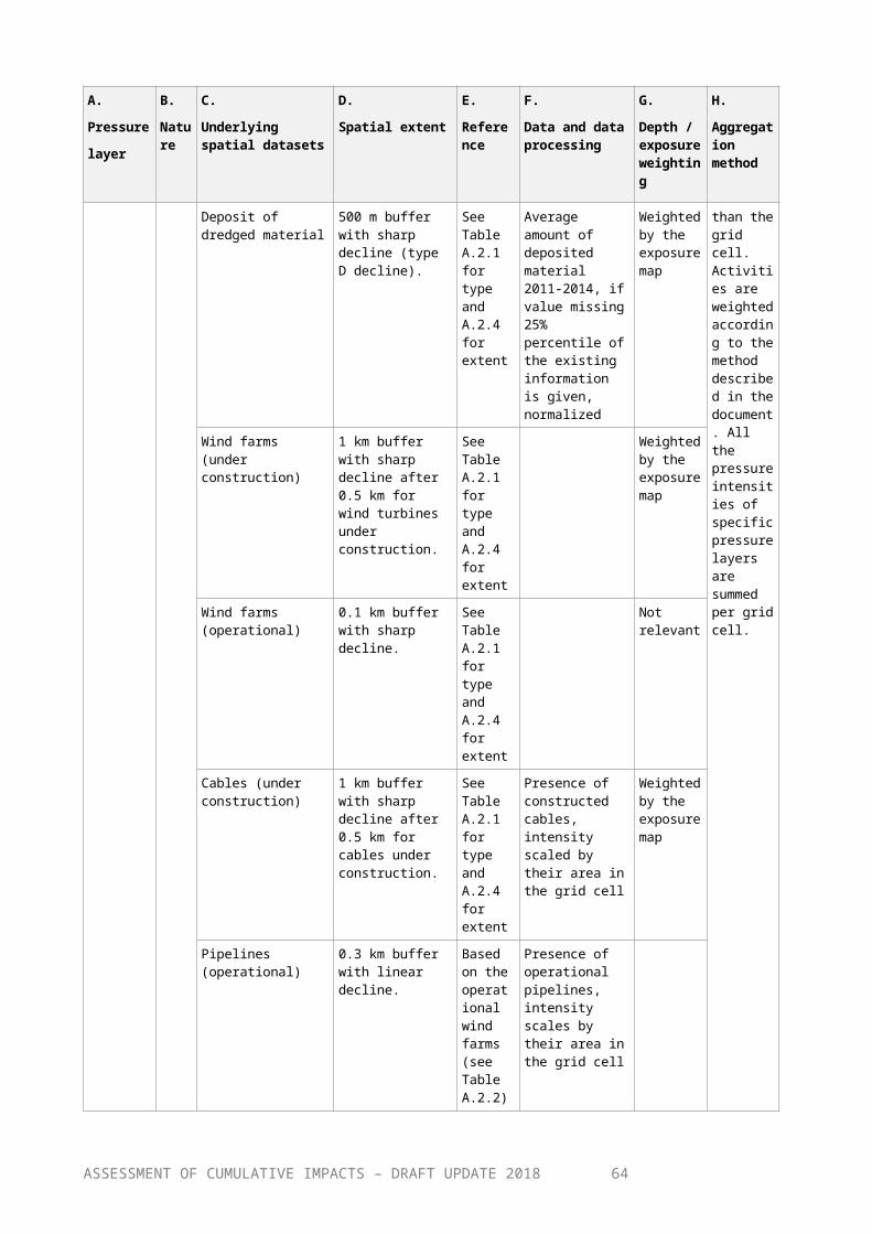
Table A.2.2. Spatial extent of physical disturbance from different human activities. The extents were estimated as the distance from the activity at which the pressure intensity can be considered negligible. Note that the estimates are also affects by hydrographic conditions, and that the estimates given here are usually applicable to exposed or semi-exposed areas. The information is based on results from the BalticBOOST project, and was used as a complement to the expert survey for processing the pressure data layers (Annex 1).

Human activity Pressure extent (specification to ecosystem component given in brackets)

Literature reference

Capital dredging 4 km (fish), 3 km (benthos), 3 km (vegetation), 3 km (water turbidity)

Lassalle et al. 1990, Morton 1996 , Kotta et al. 2009, Vatanen et al. 2012

Maintenance dredging

4 km (fish), 3 km (benthos), 3 km (vegetation), 3 km (water turbidity)

Lassalle et al. 1990, Boyd et al. 2003, Orviku et al. 2008, Vatanen et al. 2010

Sand extraction 5 km (water turbidity), 4 km (fish), 3 km (vegetation), 2 km (benthos)

Nichols et al. 1990, Boyd et al. 2003, Phua et al. 2004, Vatanen et al. 2012

Disposal of dredged matter

4 km (fish), 3 km (benthos), 3 km (vegetation), 2 km (water turbidity)

Syväranta et al. 2013, Syväranta & Leinikki 2014, Vatanen et al. 2014, Syväranta & Leinikki 2015, Vatanen et al. 2015

Shipping and ferry traffic

1 km (fish), 1 km (water turbidity, 30 m in depth), 0.5 km (vegetation), 0.3 km abrasion (substrate change)

Rytkönen et al. 2001, Vahteri & Vuorinen 2001, Soomere et al. 2003, Eriksson et al. 2004, Sandström et al. 2005, Vatanen et al. 2010, Syväranta & Vahteri 2013

Boating 0.5 km (water turbidity, 4 m in depth),

Degerman & Rosenberg 1981, Oulasvirta & Leinikki 2003, Eriksson et al. 2004, Sandström et al. 2005

Marinas 0.5 km (fish), 0.5 km (vegetation) Eriksson et al. 2004, Sandström et al. 2005; and the references in ‘Dredging’

Demersal trawling (siltation)

0.1 km

Demersal trawling (abrasion)

local

Wind turbines, oil rigs (operational)

0.1 km Eastwood et al. 2007

Wind turbines, oil rigs (construction)

300 m (wind turbines), 500 m (oil rigs)

Roth 2004, Eastwood et al. 2007, Andersson 2011, van der Wal & Tamis 2014; and the references in ‘Dredging’

Cable placement 0.5-1km Andrulewicz et al. 2003, Kogan 2006; and the references in ‘Dredging’


Summary of literature review to support the setting of sensitivity scoresThe literature to support the setting of sensitivity scores for benthic habitats with respect to the pressures ‘Physical disturbance’ and ‘Changes in Hydrological conditions’ is given in Tables A.2.3-4. Literature to support the assessment of other pressures impacting on benthic habitats is listed in Table A.2.5. The sensitivity of species groups to other pressure types based on the information in the literature review is presented in table A.2.6.

Table A.2.3. Sensitivity of benthic habitats to physical disturbance pressure based on the literature review. The sensitivities are estimated based on activities causing impacts and the recovery time. [moved from main text to Annex]

Benthic habitat

Reported impacts

Recovery Sensitivity category

References

Broad-scale seabed habitats

Infralittoral hard bottom

Strong siltation impacts.

>4 years, depends on shore exposure

High Essink 1999, Vahteri & Vuorinen 2001, Oulasvirta & Leinikki 2003, Kotta et al. 2009

Infralittoral sand

Intermediate-high siltation impacts on eelgrass

>2-6 years High Oulasvirta & Leinikki 2003, Erftemeijer et al. 2006

Infralittoral mud Vegetation and fish spawning highly impacted. Impacts not as high as on hard bottoms.

4-6 years High Oulasvirta & Leinikki 2003, Eriksson et al. 2004, Sandström et al. 2005, Munsterhjelm 2005, Torn et al. 2010, Vatanen et al. 2012

Circalittoral hard bottom

Sedimentation higher due to less wave energy and limits settlement of sessile fauna.

High Essink 1999

Circalittoral sand

Macrofauna effects after modification are strong and recovery is long.

0.5-4 years High Newell et al. 1998, Boyd et al. 2000, Dalfsen & Essink 2001, Boyd et al. 2003, Barrio Frojan et al. 2008, Frenzel et al. 2009, Manso et al. 2010, Vatanen et al. 2012, Wan Hussin et al. 2012


Circalittoral mud

Intermediate siltation impacts. Altered size distribution (juveniles die). Mortality takes place but recovery is rather fast.

typically 2.5-6 years

Moderate Essink 1999, Orviku et al. 2008, Powilleit et al. 2009, Vatanen et al. 2012

Habitat forming species

Furcellaria lumbricalis

Sedimentation effects are high.

High sensitivity

Eriksson & Johansson 2005

Zostera marina Sedimentation effects are high.

4-6 years High sensitivity

Oulasvirta & Leinikki 2003, Erftemeijer et al. 2006, Munkes et al. 2015

Charophytes Sedimentation and altered wave energy impact highly.

High sensitivity

Eriksson et al. 2004, Munsterhjelm 2005, Sandström et al. 2005, Torn et al. 2010

Mytilus edulis Sedimentation effects are high.

High sensitivity

Kotta et al. 2009

Fucus spp. No colonization and 80% loss of coverage at impact zone.

>4 years High sensitivity

Bonsdorff 1980, Bonsdorff et al. 1986, Eriksson & Johansson 2005, Vatanen et al. 2012, Syväranta et al. 2013, Syväranta & Leinikki 2015

Table A.2.4. Sensitivity of benthic habitats to ‘Changes in hydrographical conditions’ based on the literature review. The sensitivities are estimated based on activities causing impacts. [Moved from main text to annex]

Benthic habitat Reported impacts Sensitivity category

References

Broad-scale seabed habitats


Accumulation of finer sediments to landward side of coastal structures -> high biological impact on sessile species.

High Martin et al. 2005

Infralittoral sand Accumulation of finer sediments to landward side of coastal structures -> biological change. Abrasion around an installation changes seabed morphology and substrate.

Moderate Martin et al. 2005, Eastwood et al. 2007

Infralittoral mud Accumulation of finer sediments to landward side of coastal structures -> biological change. Abrasion around an installation changes seabed morphology and

Moderate Martin et al. 2005, Eastwood et al. 2007


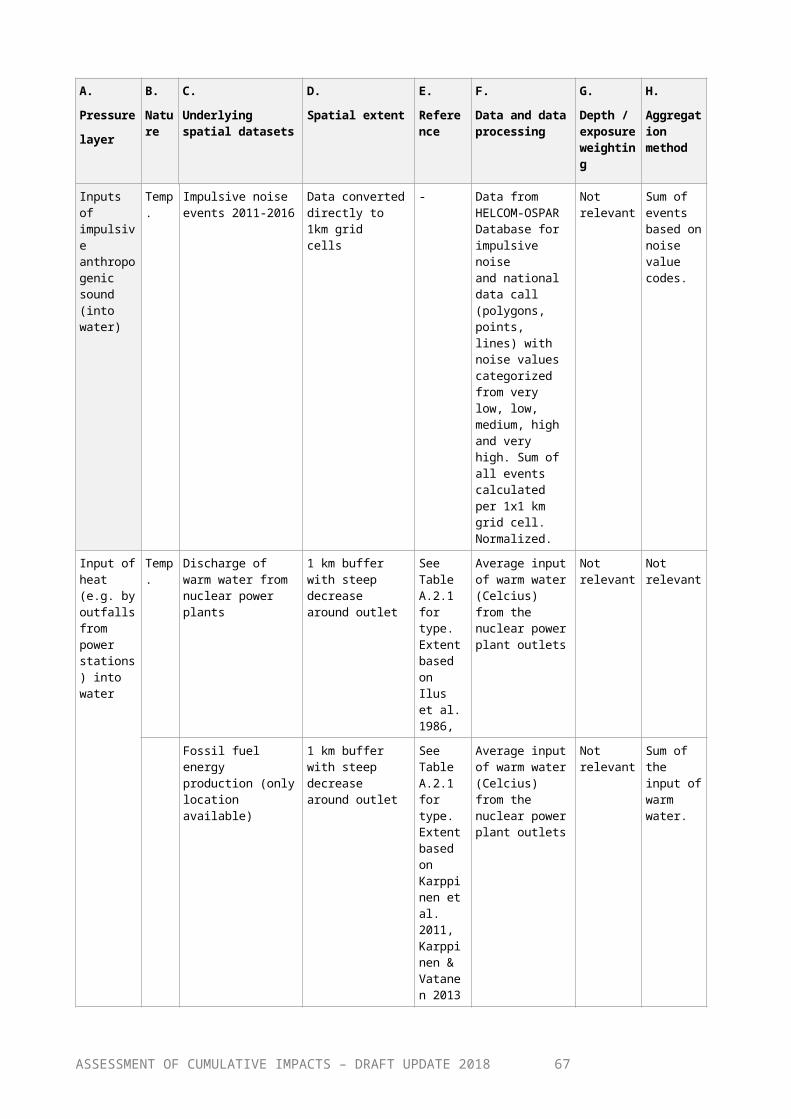
substrate.Circalittoral hard bottom

No information

Circalittoral sand Abrasion around an installation changes seabed morphology and substrate (smaller at greater depths)

Low Eastwood et al. 2007

Circalittoral mud Abrasion around an installation changes seabed morphology and substrate (smaller at greater depths).

Low Eastwood et al. 2007

Habitat forming species

Furcellaria lumbricalis

No information

Zostera marina No informationCharophytes No informationMytilus edulis No informationFucus sp. No information

Table A.2.5. Sensitivity of benthic habitats to other pressure types based on the literature review.


Infralittoral sand

Infralittoral mud

Circalittoral hard bottom

Circalittoral sand

Circalittoral mud

Input of organic matter

High (1, 9) High (1, 9) High (1,8, 9) High (1, 9) High (1, 9) High (1,8, 9)


High(2) High(2,10) High(2,5,10) High(2) High(2,10) High(2,10)

Input of nutrients Inter-mediate(3)

Inter-mediate(3)

High(3, 4) Inter-mediate(3)

Inter-mediate(3)

Inter-mediate(3)

Input of heat Inter-mediate(6)

Inter-mediate(6)

Inter-mediate(6)

Inter-mediate(6)

Inter-mediate(6)

Inter-mediate(6)

Inputs of radioactive substances

Low (7)

Input of impulsive noise

Intermediate (12)

Intermediate (12)

Intermediate (12)

Intermediate (12)

Intermediate (12)

Intermediate (12)

Input of continuous noise

Low (12) Low (12) Low (12) Low (12) Low (12) Low (12)

Input of electromagnetism

Low (11,12) Low (11,12) Low (11,12) Low (11,12) Low (11,12) Low (11,12)

(1) Recovery time of zoobenthos is 5-10 years (Bonsdorff et al. 1986).(2) Recovery time of zoobenthos is 8- >10 years (Bonsdorff et al. 1986).(3) Recovery time of zoobenthos is ca 5 years (Bonsdorff et al. 1986)(4) Macroalgal mats and anoxia cause mass mortality (Ellis et al. 2000)(5) 30-40% zoobenthos density reduction (Ellis et al. 2000)(6) Increased water temperature by 2-4 C degrees (nuclear) or 1 C degree (coal plant) in the summer until 1-1.5 km distance (Ilus et al. 1986, Karppinen & Vatanen 2013); 5-9 C degree ASSESSMENT OF CUMULATIVE IMPACTS – DRAFT UPDATE 2018

67

increase at 200 m distance outside a coal plant (Karppinen et al. 2011).(7) Increased radioactivity at 10 km distance (Ilus et al. 1986)(8) No recovery of zoobenthic community after 8 years of cessation of a fish farm in a sheltered bay (Kraufvelin et al. 2001)(9) 10-fold periphyton biomass at 500 m distance from a fish farm (Leskinen et al. 1986)(10) Near oil platforms sensitive species are progressively substituted by indifferent, tolerant and second- and first-order opportunistic species (Muxika et al. 2005, Terlizzi et al. 2008)(11) Electromagnetic effects may take place, they are stronger for cables with electrodes and weaker for bipolar cables (Andrulewicz et al. 2003)(12) Review of impacts of wind farms under construction and in operation (Bergström et al. 2014)

Table A.2..6. Sensitivity of species groups to other pressure types based on the information in the literature review.

Seals Porpoise Fish Seabirds

Input of impulsive noise High (3) High (3) High (1,2)

Input of continuous noise Low (3) Intermediate (3) Low (1,2,3)

Input of electromagnetism Low (3,4,6) Low (3,4,6) Low (3,4,6)

Disturbance of species: collision Intermediate (5)

(1, 2) Andersson (2011); (3) Bergström et al. 2014 ; (4) Andrulewicz et al. 2003; (5) Gill 2005; (6) Wilhelmsson et al. (2010)


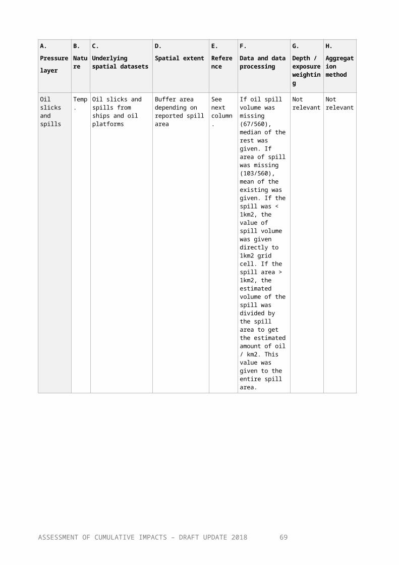
Comparison of expert survey results and literature review

Physical lossThe literature review suggested that all the sensitivity scores for the ‘physical loss’ pressure be set to ‘High’ for benthic habitats. The expert survey gave that the mean score for benthic habitats is 1.83 of the maximum 2.0, and that the experts considered benthic habitats to be highly sensitive to physical loss. For the two pelagic habitats, the expert survey gave the scores 0.4 and 0.9 and for mammals, seabirds and pelagic fish the mean score is 0.86 (range 0.5-1.2). No literature evidence suggested otherwise. Spawning areas of coastal fish (roach, pike and pikeperch, spawning among benthic vegetation) received scores 1.3-1.4 in the expert survey which is lower than findings in the literature that benthic vegetation is sensitive to physical loss. The expert survey was followed after increasing the scores by 20%.

Physical disturbance on seabedThe pressure ‘physical disturbance on seabed’ was estimated by the literature review as highly impacting and the sensitivity scores were ‘high’ in almost all cases, but the range of habitats considered in the literature study was not as wide as in the expert survey. In the expert survey, the resulting scores were quite variable for different types of habitats: the average score 1.17 (range 1.0-1.3) for all broad-scale habitats, 1.76 (range 1.6-1.9) for all habitat-forming species and 1.56 (range 1.2-1.7) for all the Natura 2000 habitats (the mean is 1.6 (range 1.5-1.7) if ‘submarine structures made by leaking gases’ is omitted). The maximum score is 2.0. The results shows that the benthic habitats are highly sensitive to this pressure. The observed variability indicated that the experts considered that the more biological elements are included in the habitat classification, the more sensitive is the habitat. For example, the habitat-forming species were considered more sensitive than the broad-scale habitats or Natura 2000 habitats. The sensitivity of pelagic habitats (surface and deep) to physical disturbance was scored as 1.0 and 0.7, respectively, indicating moderate sensitivity. The resulst of the literature review were similar, showing that the recovery after siltation and consequent turbidity is fast and therefore the sensitivity should be considered as ‘moderate’ (i.e. score 1.0). The sensitivity of mammals, fish and seabirds in the expert survey ranged between 0.5 and 1.3 (mean 0.81), likely indicating that the highly mobile species are only indirectly affected by seabed disturbance. The literature review results was in line with the expert survey, and the results from the expert survey were used.

Changes in hydrological conditionsChanges in hydrological conditions were not estimated to be as serious as the other two physical pressures according to the expert survey. The broad-scale habitats had sensitivity scores ranging between 0.9 and 1.4 (mean 1.17), indicating moderate impacts, which is partly in line with the literature review, where deeper habitats were estimated as ‘low sensitivity’ and infralittoral habitats as ‘moderate’. Pelagic habitats in surface and deep had sensitivity


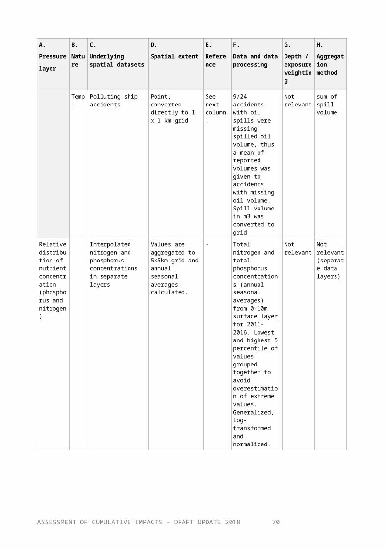
scores 0.6 and 1.3, Natura 2000 habitats ranged between 1.1 and 1.8 (mean 1.4), habitat-forming species between 1.3-1.7 (mean 1.54) and the mobile species between 0.4 and 1.2 (mean 0.72). The expert survey results were used.

Input of continuous soundSensitivity to input of continuous sound was estimated by the expert survey as highest to the marine mammals (mean 1.52), especially harbor porpoise (1.7). Fish and seabird sensitivities ranged between 0.2-0.8 (mean 0.52) and all habitats between 0-1.0 (mean 0.39). This is in line with the literature-based estimates, which suggested low sensitivity to all habitats, fish and seals. The moderate sensitivity of harbor porpoise was likely an underestimation in the literature review. The expert survey results were used.

Input of impulsive soundThe input of impulsive noise was rated rather similarly, as marine mammal sensitivity scores ranged between 1.5-1.9 (mean 1.62, harbor porpoise getting 1.9), fish and seabirds getting the scores 0.7-1.1 (mean 0.92) and all habitats between 0 and 1.0 (mean 0.41). These results are in contrast with the literature, where moderate-high sensitivity was suggested for all the ecosystem components. As the available literature was not referring to empirical results but to assumptions, the expert survey results were used.

ElectromagnetismSensitivity of all ecosystem components to electromagnetism scored between 0 and 1.0 (mean 0.54). This is in line with the literature review which estimated low sensitivity to all ecosystem components. The expert survey results were used.

Input of heatThe expert survey resulted in variable sensitivity to input of heat. Pelagic and benthic broad-scale habitats scored between 0.6 and 1.3 (mean 0.96), habitat-forming species scored between 0.9-1.6 (mean 1.3), Natura 2000 habitats between 0.9 and 1.7 (mean 1.11), fish between 0.3-0.8 (mean 0.56), seabirds between 0.3-0.6 (mean 0.4) and marine mammals between 0.2 and 0.6 (mean 0.36). Literature-based scores were obtained only for broad-scale habitats which all scored as ‘moderate’. The expert survey results were used.

Input of hazardous substances Sensitivities against input of hazardous substances depended on the ecosystem component. Pelagic and benthic broad-scale habitats ranged between 0.9-1.2 (mean 0.99), habitat-forming species ranged between 0.8-1.1 (mean 0.92), Natura 2000 habitats had sensitivities between 0.6 and 1.2 (mean 0.83), seabirds and marine mammals ranged between 1.2 and 1.6 (mean 1.44) and fish between 0.4 and 0.9 (mean 0.62). Literature-based estimates could be obtained only for sediment contamination which was considered as highly impacting for ASSESSMENT OF CUMULATIVE IMPACTS – DRAFT UPDATE 2018

70

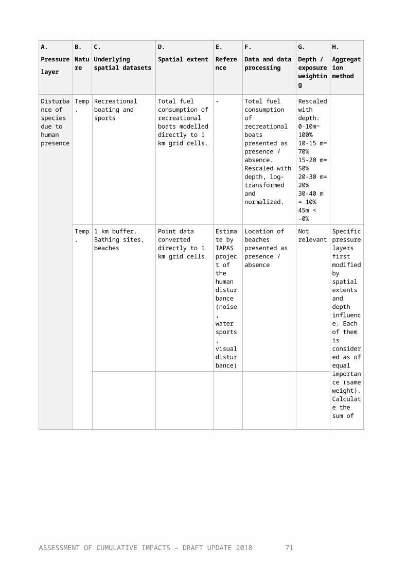
zoobenthos. The results seemed to be in contrast with the expert results which considered benthic habitats to be moderately sensitive. The difference may be due to high variability in substances and pollution levels; highly contaminated sediments may cause acute mortality whereas accumulative effects are more of a problem for long-living predators. There was also some uncertainty among experts about the effects on habitats (and associated species). The expert survey results were used as no targeted deeper review was made for contamination.

Input of nutrients (nitrogen and phosphorous)Sensitivity to input of nutrients is probably best known in the Baltic Sea. Pelagic surface and deep habitats scored 1.5 and 1.8, respectively, and the benthic broad-scale habitats scored between 1.2-1.3. Of the habitat-forming species, blue mussels scored only 0.9 whereas the plants scored between 1.3 and 1.9. Natura 2000 habitats scored between 1.2 and 1.6 (mean 1.4) and seabirds and mammals between 0.2 and 0.5. Among the fish, the deep-water and vegetation spawners scored high (1.3-1.7) whereas other fish were estimated to have rather low sensitivity (0.5-0.7). According to the scarce literature information, benthic broad-scale habitats were mostly scored as ‘moderately sensitive’, which is in line with the expert survey. The expert survey results were used.

Input of radionuclidesInput of radionuclides was not considered as highly impacting in the survey, as the expert scores ranged among all the ecosystem components only between 0 and 1.2 (mean 0.44). In the literature review there was only one reference, which indicated moderate sensitivity for broad-scale habitats. The expert survey results were used.

Oil slicks and spillsSensitivity of broad-scale habitats to oil slicks and spills was estimated to range between 0.9 and 1.7 (mean 1.28) and the highest sensitivity was estimated for infralittoral hard bottoms. Habitat-forming species scored between 1.4 and 1.6 , Natura 2000 habitats between 1.5-1.9, fish between 0.5 and 1.7 (higher values for vegetation spawners), seabirds between 1.9-2.0 and marine mammals between 1.3 and 1.6. The scores showed a rather clear pattern for higher sensitivity in hard bottoms, reefs and vegetation and very high and obvious sensitivity of seabirds. No literature information was available through the review and the expert survey results were used.

Input of litterThe expert survey showed low sensitivity of most of the ecosystem components. Exceptions were seabirds and marine mammals, which scored between 0.9-1.2, while other ecosystem components scored between 0.1 and 0.8 (mean 0.42). No literature information was available through the review and the expert survey results were used.


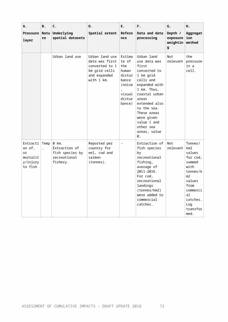
Input of organic matterSensitivity to input of organic matter was relatively clear ‘moderate’ to the broad-scale habitats, Natura 2000 habitats, fish spawning habitats and habitat-forming species (0.8-1.4, mean 1.11). Marine mammals, seabirds and fish scored only 0.5 in average (0.3-1.1). According to the literature survey, organic enrichment has higher impacts and longer recovery times in case of benthic habitats than what is estimated by the expert survey. This pressure layer was not included in the Baltic Sea Impact Index.

Disturbance to speciesMarine mammals and seabirds were estimated to be sensitive to human disturbance (1.0-1.8, mean 1.36). Fish had clearly lower scores (0.4-1.3, mean 0.81) and the habitats were estimated between 0.2-1.2 (mean 0.67). No literature information was available through the review and the expert survey results were used.

Extraction and injury to fishSensitivity of fish to fish extraction was estimated to score 1.57 in average (1.2-2.0). Marine mammals and seabirds scored to this pressure – being indirectly impacted by decreased prey – between 0.7 and 1.5 (mean 1.13). Habitats scored between 0.3 and 1.1 (mean 0.74). No literature information was available through the review and the expert survey results were used.

Hunting of seals and seabirdsHunting of seals and seabirds (including predator control) was estimated to score 1.9 in average (range 1.6-2.0) for seals and 1.65 in average for seabirds (1.6-1.7). Sensitivity of fish to this pressure was obviously low (0-0.7, mean 0.29). Habitats scored between 0.2 and 1.5 (mean 0.7). No literature information was available through the review. As this pressure describes hunting, bycatch of harbor porpoise was not included in this pressure but in ‘Extraction and injury to fish’.

Introduction of non-indigenous species and translocations of native speciesSensitivity of ecosystem components to introduction of non-indigenous species (NIS) and translocations of native species was generally scored in the survey as ‘moderate’ (range 0.3-1.4, mean 0.88). Pelagic and benthic habitats as well as Natura 2000 habitats were estimated as more sensitive (mean 1.04, range 0.7-1.4) than the mobile species (range 0.4-1.1, mean 0.69). This is rather obvious as most of the NIS are small and are found to affect invertebrate communities rather than larger species. However, it seems that the experts did not consider the terrestrial NIS (American mink and raccoon dog) which have heavy impacts on seabird populations. Terrestrial NIS are not part of the impact assessment and therefore it was not necessary to change the seabird sensitivity score, but this should be kept in mind in descriptive assessments of NIS. No literature information was available through the review. As ASSESSMENT OF CUMULATIVE IMPACTS – DRAFT UPDATE 2018

72

literature has shown that the common invasive non-indigenous species, such as round goby and mud crab have strong impacts to habitats formed by blue mussels and vegetation (Kuhns & Berg 1999, Lederer et al. 2008), the sensitivity scores of benthic habitat-forming species (ranging from 0.7 to 0.9) in the experts survey were increased by 50% (to ranging from 1.0 to 1.4).

Changes in climatic conditionsSensitivity of the Baltic Sea habitats and species to changes in climatic conditions was estimated in the expert survey as ‘moderate’ (range 0.5-1.7, mean 1.01). The highest sensitivity (1.7) was estimated for ringed seal distribution and deep water conditions, which are both well-known phenomenon in the region. The lowest sensitivity (0.3-0.5) was estimated for freshwater fish species living in the coastal waters, where salinity is expected to decrease.

AcidificationThe other climate-related pressure acidification, had higher variability in the responses (0.3-2.0, mean 1.02). The highest sensitivity was generally given to habitats where there are sessile species (e.g. submarine structures made by leaking gases, infralittoral hard bottoms, esker islands, boreal Baltic islets), but this pattern was not consistent. No literature information was available through the review. This pressure layer was not included in the Baltic Sea Impact Index.
