Sulfate mineral scaling during the production of geothermal energy from sedimentary basin formation brines:

A case study at the Groß Schönebeck in-situ geothermal laboratory, Germany

A dissertation submitted to the Fachbereich Geowissenschaften

der Freien Universität Berlin for the degree of Doctor of Science

-Doktor rerum naturalium-

presented by

Jonathan C. Banks, M.S.T.

Berlin, 2013

ii

3

Evaluators: Prof. Dr. Michael Schneider, Freie Universität Berlin

Prof. Dr. Jörg Erzinger, Universität Potsdam Date of Oral Defense (Disputation): 9. April 2013 FU Berlin 74-100 Malteserstr. 12249 Berlin

4

5

Declaration of authenticity and originality I, Jonathan C. Banks, declare that the work contained in this document is my own creation. No person

other than myself prepared any part of this document. All assistance I have received in the

performance of this study is duly cited, according to the accepted standards and practices of the

scientific community, in the acknowledgements and reference section of this work. At the time of

submission to the Fachbereich Geowissenschaften der Freien Universität Berlin, no part of this work

has been submitted for publication in a peer-reviewed journal. To the best of my knowledge, no such

study has been previously conceptualized, performed or published. Signed____________________________________________________________________

Location/Date

6

Dedication This dissertation is dedicated to Bhagavan Shri Krishna, the source and the goal of all knowledge:

yat karoṣi yad aśnāsi yaj juhoṣi dadāsi yat

yat tapasyasi kaunteya tat kuruṣva mad-arpaṇam

“Whatever you do, whatever you eat, whatever you offer or give away, and whatever austerities you perform — do that, O son of Kuntī, as an offering to Me. “ –Bhagavad-Gita 9.27

vii

8

9

Acknowledgments An undertaking of this magnitude cannot be accomplished alone, and I am grateful to many people for helping me complete this dissertation. In particular, I would like to thank:

• Drs. Simona Regenspurg and Harald Milsch at the GFZ Potsdam for the day-to-day

supervision of the scientific aspects of this work.

• Prof. Dr. Michael Schneider at the FU Berlin for signing off on this project as legitimate

doctoral research and for supervising my Promotionsverfahren.

• The Deutsche GeoForschungsZentrum Potsdam, specifically Prof. Dr. Ernst Huenges and Dr.

Ali Saadat, for ongoing investment in this research and for showing exceptional tolerance and flexibility regarding my shortcomings as an employee.

• Ronny Giese, Christian Cunow, Alexander Reichardt, Andreas Kratz, Tanja Ballerstadt, Liane

Liebeskind and all of the Azubis in our technicians’ office at the GFZ. A bunch of regular Macgyvers, ya’ll are.

• Ansgar Schepers, Andhika Muhamad, Dejene Driba, Maren Brehme, Ulrike Hoffert and

Elvira Feldbusch for sharing the limited lab space with me.

• Dr. Elke Heyde at the FU Berlin for assisting with all of the fluid phase analyses.

• Rudolf Naumann and Andrea Gottsche at the GFZ Potsdam for assisting with the XRF and

XRD analyses.

• Dr. Helga Kemnitz and Ilona Schäpers at the GFZ Potsdam and Dr. Ann Heatherington at the

University of Florida for assisting with SEM analyses.

• Sophia Wagner for significant contributions to the fieldwork at Groß Schönebeck, including

preparing the XRD, XRF and SEM samples for analysis.

• Karl Galgana Schimkowski for helping me translate the abstract into German.

• Dr. Kenneth R. Valpey at the Oxford Center for Hindu Studies for holding the light at the end

of the tunnel.

• Susan, David, Jennifer, Jeffrey, Shalima, Eveanna and Milo Banks simply for being the people

who are always there, through high tides and low tides. Thirty-five years is far too short a time to live amongst such excellent and admirable hobbits.

10

11

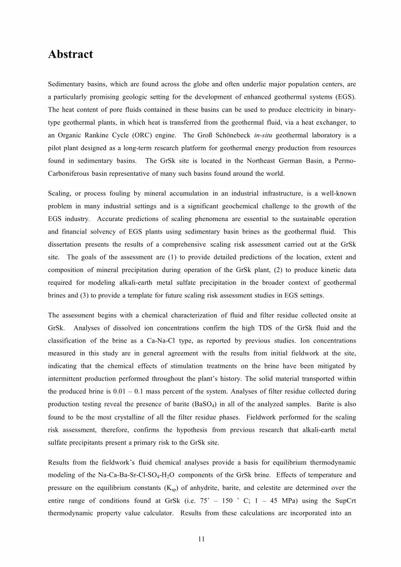
Abstract Sedimentary basins, which are found across the globe and often underlie major population centers, are

a particularly promising geologic setting for the development of enhanced geothermal systems (EGS).

The heat content of pore fluids contained in these basins can be used to produce electricity in binary-

type geothermal plants, in which heat is transferred from the geothermal fluid, via a heat exchanger, to

an Organic Rankine Cycle (ORC) engine. The Groß Schönebeck in-situ geothermal laboratory is a

pilot plant designed as a long-term research platform for geothermal energy production from resources

found in sedimentary basins. The GrSk site is located in the Northeast German Basin, a Permo-

Carboniferous basin representative of many such basins found around the world.

Scaling, or process fouling by mineral accumulation in an industrial infrastructure, is a well-known

problem in many industrial settings and is a significant geochemical challenge to the growth of the

EGS industry. Accurate predictions of scaling phenomena are essential to the sustainable operation

and financial solvency of EGS plants using sedimentary basin brines as the geothermal fluid. This

dissertation presents the results of a comprehensive scaling risk assessment carried out at the GrSk

site. The goals of the assessment are (1) to provide detailed predictions of the location, extent and

composition of mineral precipitation during operation of the GrSk plant, (2) to produce kinetic data

required for modeling alkali-earth metal sulfate precipitation in the broader context of geothermal

brines and (3) to provide a template for future scaling risk assessment studies in EGS settings.

The assessment begins with a chemical characterization of fluid and filter residue collected onsite at

GrSk. Analyses of dissolved ion concentrations confirm the high TDS of the GrSk fluid and the

classification of the brine as a Ca-Na-Cl type, as reported by previous studies. Ion concentrations

measured in this study are in general agreement with the results from initial fieldwork at the site,

indicating that the chemical effects of stimulation treatments on the brine have been mitigated by

intermittent production performed throughout the plant’s history. The solid material transported within

the produced brine is 0.01 – 0.1 mass percent of the system. Analyses of filter residue collected during

production testing reveal the presence of barite (BaSO4) in all of the analyzed samples. Barite is also

found to be the most crystalline of all the filter residue phases. Fieldwork performed for the scaling

risk assessment, therefore, confirms the hypothesis from previous research that alkali-earth metal

sulfate precipitants present a primary risk to the GrSk site.

Results from the fieldwork’s fluid chemical analyses provide a basis for equilibrium thermodynamic

modeling of the Na-Ca-Ba-Sr-Cl-SO4-H2O components of the GrSk brine. Effects of temperature and

pressure on the equilibrium constants (Ksp) of anhydrite, barite, and celestite are determined over the

entire range of conditions found at GrSk (i.e. 75˚ – 150 ˚ C; 1 – 45 MPa) using the SupCrt

thermodynamic property value calculator. Results from these calculations are incorporated into an

xii

equilibrium model created with the Geochemists’ Workbench (GWB) software. Based on the Pitzer

theory of specific ion interactions, the model calculates changes in the brine’s pH, species activities,

mineral saturation states, stable mineral phase assemblages and projected reaction paths across the

relevant (T, p) range. Pressure is found to have little effect on the system’s equilibrium. Increasing

the temperature from 75˚ C to 150˚ C moves the GrSk fluid from the barite stability field to the

anhydrite stability field. Celestite is only found to be stable at high temperatures and low barium

concentrations. Varying SO4 concentrations have no effect on barite saturation until SO4

concentrations drop below 0.5 millimolar (mM). Anhydrite saturation is directly tied to the SO4

concentration.

Equilibrium models have limited predictive value in determining the extent of scaling risks because

they do not take into account precipitation reaction kinetics. Kinetic parameters for sulfate mineral

precipitation from mixed electrolyte solutions at elevated temperatures and pressures are practically

non-existent in the literature. These kinetic parameters, therefore, are experimentally determined in

this study for anhydrite, barite and celestite precipitation from a synthetic geothermal brine analogous

to that found at GrSk and representative of sedimentary basin brines found around the world. To

perform these experiments, a batch reactor system able to operate at high temperatures and pressures

in the presence of an aggressive, corrosion inducing fluid is designed, constructed and tested.

Precipitation kinetics are measured at 75˚ C and 150 ˚ C. Barite is the only mineral appearing in the

filter residue at both temperatures. Strontium and calcium are incorporated into the barite crystals as

accessory cations. The precipitation is a 2nd order reaction, with rate constants of 0.045 and 0.025 at

75˚ C and 150˚ C, respectively, and units of [kg of brine•millimoles of precipitant-1•seconds-1]. The

change in the filter residue’s reactive surface area over time is also semi-quantitatively determined via

optical and geometric methods using a scanning electron microscope (SEM).

Once the necessary kinetic parameters are determined, it is possible to predict the location, extent and

composition of mineral precipitation within the GrSk infrastructure. The GrSk fluid’s chemical

behavior during production and reinjection is described with the use of 1-D reactive transport models

constructed with the GWB. All modeled scenarios show preferential formation of the mineral

precipitants in the upstream direction of the flow, rather than diffusely throughout the system. Flow

rates varying between 25 and 75 m3/h have negligible effect on the overall precipitation behavior.

Results from the reactive transport models show that barite dominates the system at the onset of

precipitation, with anhydrite becoming prominent on the hot side of the heat exchanger after at least 6

hours of production. Only barite is expected to appear on the cold side of the heat exchanger, although

to a much lesser extent (up to 5 orders of magnitude) by mass than on the hot side of the heat

exchanger. Precipitant forms fast enough to nearly completely block the inflow to the system in as

little as 5 days of production at 50 m3/h, assuming precipitated material is not removed from the

system, via, for example, a filtration system. Within this time frame, nearly 60 g of precipitant per m3

13

of produced brine are predicted to form in the system, practically all of which is in the first ~250 m of

the ~1200 m flow path from the production pump to the heat exchanger.

In conclusion, all of the results from this study confirm that alkali earth metal sulfate scaling,

predominated by barite, is a primary scaling risk in the GrSk system. Caution, however, should be

taken when using the reactive transport model as a true predictive tool. The model only considers the

scenario where precipitating minerals are not removed from the system. The online filtration system

at GrSk will reduce the rate at which minerals accumulate in the infrastructure.

14

Zusammenfassung Sedimentbecken, die weltweit und oftmals unter großen Ballungszentren auftreten, sind besonders

vielversprechende geologische Standorte zur Erschließung von enhanced geothermal systems. Der

Wärmegehalt von in diesen Becken enthaltenen Porenflüssigkeiten kann zur Erzeugung von

Elektrizität in Binärtyp-Geothermie-Kraftwerken eingesetzt werden, in denen Wärme

aus geothermischen Fluiden mit Hilfe eines Wärmetauschers in eine Organic Rankine Cycle-Anlage

überführt wird. Das Groß Schönebeck in-situ geothermal laboratory ist ein Pilot-Kraftwerk, das als

Langzeit-Forschungs-Plattform für geothermischen Energieerzeugung konzipiert ist, in Bezug auf

Ressourcen, die in Sedimentbecken vorliegen. Das GrSk liegt im Nordostdeutschen Becken, einem

permokarbonen Becken, das repräsentativ für viele solcher weltweit vorkommenden Becken ist.

Scaling ist ein sehr bekanntes Problem industrieller Anlagen und stellt eine bedeutende geochemische

Herausforderung für das Wachstum der EGS-Industrie dar. Verlässliche Voraussagen über das

Vorkommen von Scaling oder Fouling durch Mineralablagerungen in industrieller Infrastruktur sind

von essenzieller Bedeutung für den nachhaltigen Betrieb und die finanzielle Solvenz von EGS-

Anlagen, die Sedimentbecken Formationswasser als geothermisches Wasser nutzen. Diese

Dissertation stellt die Ergebnisse einer umfangreichen, in der GrSk-Anlage ausgeführten Scaling-

Risiko-Einschätzung vor.

Die Ziele der Einschätzung sind (1) detailierte Voraussagen zu treffen über die Lage, das Ausmaß und

die Zusammensetzung von Mineralausfällungen während des Betriebs der GrSk-Anlage, (2) kinetische

Daten zu generieren, die nötig sind, um den Niederschlag von Erd-alkali-Sulfaltmineralen im weiteren

Kontext von geothermalen Solen zu modellieren, (3) eine Mustervorlage zu schaffen für zukünftige

Studien zur Scaling-Risikobewertung im Kontext von EGS. Die Einschätzung beginnt mit einer

chemischen Charakterisierung von Flüssigkeit und Filtrat, das im GrSk vor Ort gesammelt wurde.

Analysen der gelösten Ionen-Konzentrationen bestätigen den hohen TDS der Flüssigkeit aus dem

GrSk und die Klassifizierung der Sole als Ca-Na-Cl-Typ, wie in früheren Berichten dargelegt. Die in

dieser Studie gemessenen Ionen-Konzentrationen stimmen im Großen und Ganzen mit den

Ergebnissen anfänglicher Feldforschung vor Ort überein, was darauf deutet, dass die chemischen

Effekte der Stimulationsbehandlungen der Sole durch die im Laufe der Geschichte der Anlage

unregelmäßig unterbrochene Förderung abgemildert wurden. Der in der produzierten Sole

transportierte Feststoffgehalt beläuft sich auf 0,01-0,1 Masse-Prozent des Systems. Analysen von

Filtrat, das während des Fördertests gesammelt wurde, zeigt das Vorkommen von Baryt (BaSO4) in

allen analysierten Proben. Baryt stellt sich auch unter allen Filtratphasen als dasjenige mit dem

höchsten Kristallinitätsgrad heraus. Die für die Scaling-Risiko-Einschätzung durchgeführte

Feldforschung bestätigt daher die Hypothese, dass alle Ausfällungen aus Erdalkalimetallsufaten eine

große Bedrohung für die GrSk-Anlage darstellen.

15

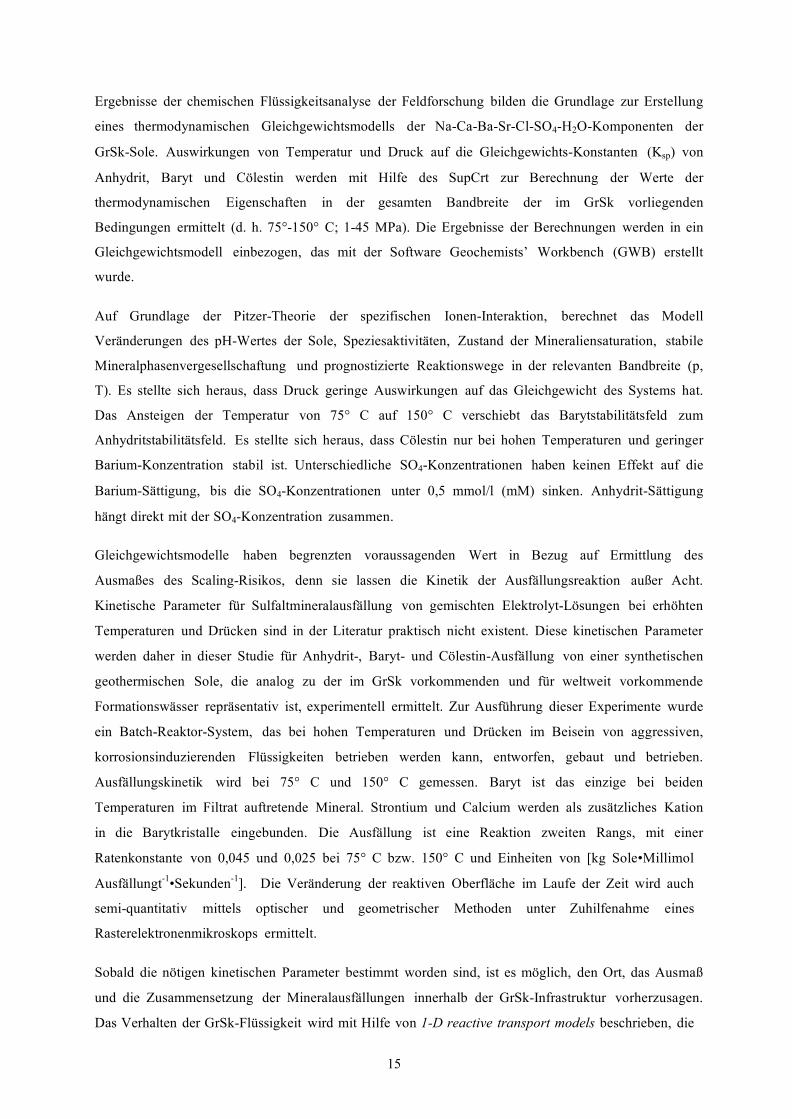
Ergebnisse der chemischen Flüssigkeitsanalyse der Feldforschung bilden die Grundlage zur Erstellung

eines thermodynamischen Gleichgewichtsmodells der Na-Ca-Ba-Sr-Cl-SO4-H2O-Komponenten der

GrSk-Sole. Auswirkungen von Temperatur und Druck auf die Gleichgewichts-Konstanten (Ksp) von

Anhydrit, Baryt und Cölestin werden mit Hilfe des SupCrt zur Berechnung der Werte der

thermodynamischen Eigenschaften in der gesamten Bandbreite der im GrSk vorliegenden

Bedingungen ermittelt (d. h. 75°-150° C; 1-45 MPa). Die Ergebnisse der Berechnungen werden in ein

Gleichgewichtsmodell einbezogen, das mit der Software Geochemists’ Workbench (GWB) erstellt

wurde.

Auf Grundlage der Pitzer-Theorie der spezifischen Ionen-Interaktion, berechnet das Modell

Veränderungen des pH-Wertes der Sole, Speziesaktivitäten, Zustand der Mineraliensaturation, stabile

Mineralphasenvergesellschaftung und prognostizierte Reaktionswege in der relevanten Bandbreite (p,

T). Es stellte sich heraus, dass Druck geringe Auswirkungen auf das Gleichgewicht des Systems hat.

Das Ansteigen der Temperatur von 75° C auf 150° C verschiebt das Barytstabilitätsfeld zum

Anhydritstabilitätsfeld. Es stellte sich heraus, dass Cölestin nur bei hohen Temperaturen und geringer

Barium-Konzentration stabil ist. Unterschiedliche SO4-Konzentrationen haben keinen Effekt auf die

Barium-Sättigung, bis die SO4-Konzentrationen unter 0,5 mmol/l (mM) sinken. Anhydrit-Sättigung

hängt direkt mit der SO4-Konzentration zusammen.

Gleichgewichtsmodelle haben begrenzten voraussagenden Wert in Bezug auf Ermittlung des

Ausmaßes des Scaling-Risikos, denn sie lassen die Kinetik der Ausfällungsreaktion außer Acht.

Kinetische Parameter für Sulfaltmineralausfällung von gemischten Elektrolyt-Lösungen bei erhöhten

Temperaturen und Drücken sind in der Literatur praktisch nicht existent. Diese kinetischen Parameter

werden daher in dieser Studie für Anhydrit-, Baryt- und Cölestin-Ausfällung von einer synthetischen

geothermischen Sole, die analog zu der im GrSk vorkommenden und für weltweit vorkommende

Formationswässer repräsentativ ist, experimentell ermittelt. Zur Ausführung dieser Experimente wurde

ein Batch-Reaktor-System, das bei hohen Temperaturen und Drücken im Beisein von aggressiven,

korrosionsinduzierenden Flüssigkeiten betrieben werden kann, entworfen, gebaut und betrieben.

Ausfällungskinetik wird bei 75° C und 150° C gemessen. Baryt ist das einzige bei beiden

Temperaturen im Filtrat auftretende Mineral. Strontium und Calcium werden als zusätzliches Kation

in die Barytkristalle eingebunden. Die Ausfällung ist eine Reaktion zweiten Rangs, mit einer

Ratenkonstante von 0,045 und 0,025 bei 75° C bzw. 150° C und Einheiten von [kg Sole•Millimol

Ausfällungt-1•Sekunden-1]. Die Veränderung der reaktiven Oberfläche im Laufe der Zeit wird auch

semi-quantitativ mittels optischer und geometrischer Methoden unter Zuhilfenahme eines

Rasterelektronenmikroskops ermittelt.

Sobald die nötigen kinetischen Parameter bestimmt worden sind, ist es möglich, den Ort, das Ausmaß

und die Zusammensetzung der Mineralausfällungen innerhalb der GrSk-Infrastruktur vorherzusagen.

Das Verhalten der GrSk-Flüssigkeit wird mit Hilfe von 1-D reactive transport models beschrieben, die

16

mit GWB erstellt wurden. Alle erstellten Szenarien zeigen eine Bildung von Mineralausfällungen

vornehmlich in Richtung der Anströmung statt einer diffusen Verteilung im System. Die zwischen 25

und 75 m3/h schwankenden Durchflussmengen haben einen vernachlässigbaren Effekt auf das

Gesamtausfällungsverhalten. Ergebnisse der reaktiven Transportmodelle zeigen, dass zu Beginn der

Ausfällung Baryt im System dominiert, wohingegen Anhydrit auf der heißen Seite des

Wärmetauschers nach mindestens 6 Stunden der Förderung vorherrscht. Erwartungsgemäß sollte nur

Baryt auf der kalten Seite des Wärmetauschers auftreten, obwohl massemäßig in viel geringerem

Ausmaß (bis zu 5 Größenordnungen) als auf der heißen Seite des Wärmetauschers. Ausfällungen

bilden sich schnell genug, um den Zufluss ins System in lediglich 5 Tagen der Förderung bei 50 m3/h

vollständig zu blockieren, vorausgesetzt, ausgefälltes Material wird nicht aus dem System entfernt.

Innerhalb dieses Zeitrahmens bilden sich voraussichtlich fast 60 g Ausfällungen pro m³ produzierter

Sole im System, wovon sich praktisch alles in den ersten ~250 m des ~1200 m langen

Strömungsweges von der Förderpumpe zum Wärmetauscher befindet.

xvii

Table of Contents Declaration of authenticity and originality ...................................................................................... v Dedication ............................................................................................................................. ............ vii Acknowledgments ............................................................................................................................ . ix Abstract ...................................................................................................................... ........................ xi Zusammenfassung .......................................................................................................................... . xiv List of Figures ............................................................................................................................. ..... xix List of Tables ............................................................................................................................. ..... xxii List of Abbreviations and Symbols............................................................................................. . xxiii

1. Introduction ........................................................................................................................1 1.1 Geothermics as viable renewable energy in the 21st century ................................................ 2 1.2 The Groß Schönebeck in-situ Geothermal Laboratory ........................................................ 3 1.3 Scaling ............................................................................................................................. ........... 8 1.4 Goals of present study ............................................................................................................. . 9

2. Characterization of solid and liquid phases sampled during production testing at the Groß Schönebeck in-situ geothermal laboratory .................................................................13

2.1 Introduction............................................................................................................................ . 14 2.2 Methods ............................................................................................................................. ...... 14

2.2.1 Fluid sampling .................................................................................................................. . 14 2.2.2 Fluid Preparation .............................................................................................................. . 15 2.2.3 Solid phase sampling and preparation .............................................................................. . 16 2.2.4 Sample Analysis ............................................................................................................... . 16

2.3 Results & Discussion.............................................................................................................. . 17 2.3.1 Fluid chemical composition.............................................................................................. . 17 2.3.2 Mass fraction of solid phase in produced GrSk brine........................................................ 23 2.3.3 Chemical analyses of filter residue from the GrSk in-line filtration system ..................... 24 2.3.4 Mineralogical analyses of filter residue from the GrSk in-line filtration system .............. 28

2.4 Conclusion ............................................................................................................................. .. 33

3. Ion activities and mineral solubilities in the Na-Ca-Ba-Sr-Cl-SO4-H2O system at conditions found in the Groß Schönebeck geothermal loop ...............................................35

3.1 Introduction............................................................................................................................ . 36 3.2 Methods ............................................................................................................................. ...... 39

3.2.1 Calculating effects temperature and pressure on the logKsp of anhydrite and barite......... 39 3.2.2 Aqueous speciation of the GrSk brine from 25˚ C to 150˚ C ............................................ 39 3.2.3 Stable phase assemblages ................................................................................................. . 40 3.2.4 Polythermal reaction path model ...................................................................................... . 40

3.3 Results ............................................................................................................................. ......... 41 3.3.1 Temperature and pressure effects on the logKsp of anhydrite, barite and celestite............ 41 3.3.2 Aqueous speciation as a function of temperature in the Na-Ca-Ba-Sr-Cl-SO4-H2O system at GrSk concentrations .................................................................................................................. . 43 3.3.3 Stable phase assemblages along the GrSk geothermal loop .............................................. 45 3.3.4 Reaction path model ......................................................................................................... . 46

3.4 Discussion ............................................................................................................................. ... 47 3.5 Conclusion ............................................................................................................................. .. 50

18

4. The kinetics of alkali earth metal sulfate precipitation in a synthetic geothermal brine..........................................................................................................................................51

4.1 Introduction............................................................................................................................ . 52 4.2 Methods ............................................................................................................................. ...... 53

4.2.1 The method of integrated rates .......................................................................................... 53 4.2.2 Experimental Method ....................................................................................................... . 55

4.2.2.1 Experimental infrastructure ...................................................................................................... . 56 4.2.2.2 Experimental Solutions ............................................................................................................. . 58 4.2.2.3 Experimental Procedure............................................................................................................ . 59

4.2.3 Analytical methods ........................................................................................................... . 59 4.2.4 Mass balancing and determining the kinetic rate law parameters ..................................... 61

4.3 Results ............................................................................................................................. ......... 61 4.3.1 Mass fractions and molal quantities of precipitants over time .......................................... 61 4.3.2 Fitting experimental data to the integrated rate laws’ linear form..................................... 63 4.3.3 Filter residue analysis with scanning electron microscopy ............................................... 67

4.3.3.1 Mineralogical and chemical composition of the filter residue .................................................. 67 4.3.3.2 Crystal growth........................................................................................................................... . 67 4.3.3.3 Estimating changes in specific reactive surface area. ................................................................ 72

4.4 Discussion ............................................................................................................................. ... 72 4.4.1 Effects of temperature on reaction rate and stable phase assemblage ............................... 72 4.4.2 Evolution and mechanisms of crystal growth .................................................................... 73

4.5 Conclusions............................................................................................................................. . 74

5. 1-D reactive transport models of alkali earth metal sulfate scaling risks in the Groß Schönebeck in-situ geothermal laboratory ...........................................................................76

5.1 Introduction............................................................................................................................ . 77 5.2 Model Descriptions ................................................................................................................ . 78 5.3 Results & Discussion.............................................................................................................. . 80

5.3.1 Flow from the production pump to the heat exchanger ..................................................... 80 5.3.2 Flow within the heat exchanger ......................................................................................... 84 5.3.3 Flow over the entire surface infrastructure ........................................................................ 88

5.4 Conclusion ............................................................................................................................. .. 92

6. Conclusion.........................................................................................................................93 6.1 Summary of Major Results .................................................................................................... 94 6.2 Limitations............................................................................................................................. .. 97 6.3 Broader impacts ..................................................................................................................... . 98 6.4 Suggestions for further research ........................................................................................... 99 References ............................................................................................................................. .......... 100 Appendix A: Selected data tables ................................................................................................. 115 Appendix B: Selected photomicrographs of experimentally formed alkali earth metal sulfate mineral precipitants ...................................................................................................................... . 121

19

List of Figures FIGURE 1.1: NETWORK OF SEDIMENTARY BASINS COMPRISING THE CENTRAL

EUROPEAN BASIN SYSTEM (CEBS; FROM VAN WEES ET AL., 2000). 4 FIGURE 1.2: STRATIGRAPHIC COLUMN SHOWING THE GEOLOGIC SETTING OF THE

GRSK IN-SITU GEOTHERMAL LABORATORY. 6 FIGURE 1.3: FLOW CHART DEPICTING THE PROCESS FOR EVALUATING SCALING

RISKS IN GEOTHERMAL SYSTEMS. 10 FIGURE 2.1: BIAR SYSTEM FOR SAMPLING CORROSIVE FLUIDS FROM THE

GEOTHERMAL PRODUCTION LINE UNDER OXYGEN-FREE CONDITIONS. 15 FIGURE 2.2: FILTER BAGS (LEFT) AND CLOSE-UP OF FILTER RESIDUE (RIGHT) FROM THE

GRSK IN-LINE FILTRATION SYSTEM. 16 FIGURE 2.3: EXAMPLES OF PREPARED SAMPLES FOR FILTER RESIDUE CHEMICAL

ANALYSIS VIA XRF (LEFT) AND FILTER RESIDUE MINERALOGY ANALYSIS VIA XRD (RIGHT). 17

FIGURE 2.4 IONIC CONCENTRATIONS OF A. ALKALI AND ALKALI EARTH METALS, B. TRANSITION, POOR AND NON-METALS AND C. ANIONS MEASURED DURING PRODUCTION TESTING AT THE GRSK SITE. 19

FIGURE 2.5: RESULTS OF GRSK FLUID COMPOSITION ANALYSES PLOTTED AS MOLAR PERCENTAGES IN TERNARY SYSTEMS. 21

FIGURE 2.6: MASS FRACTION OF SOLID MATERIAL IN THE GRSK BRINE VERSUS TEMPERATURE DURING PRODUCTION. 23

FIGURE 2.7A-C: PLOTS OF MOLAR RELATIONSHIPS BETWEEN PRECIPITATED SPECIES MEASURED BY XRF ANALYSIS. 26

FIGURE 2.7D-F: PLOTS OF MOLAR RELATIONSHIPS BETWEEN PRECPITATED SPECIES MEASURED BY XRF ANALYSIS. D. S-CL SYSTEM E. PB-CU SYSTEM F. FE-PB-CU SYSTEM. 27

FIGURE 2.8: X-RAY DIFFRACTION PATTERNS FOR SOLID MATERIAL TAKEN FROM THREE 2 µM FILTERS AND SIX 10µM FILTERS 29

FIGURE 2.9A-B: PHOTOMICROGRAPHS OF (1) WEAKLY CRYSTALLINE AGGREGATE OF SOLIDS AND (2) IRON OXIDE, WITH ACCOMPANYING EDX SPECTROGRAPHS, COLLECTED FROM THE IN-LINE GRSK FILTRATION SYSTEM DURING PRODUCTION TESTING IN 2011. 30

FIGURE 2.10: PHOTOMICROGRAPH OF LAURIONITE WITH COPPER AND BARITE, COLLECTED FROM THE IN-LINE GRSK FILTRATION SYSTEM DURING PRODUCTION TESTING IN 2011. 31

FIGURE 2.11: PHOTOMICROGRAPHS OF WELL-CRYSTALLIZED BARITE, WITH ACCOMPANYING EDX SPECTROGRAPHS, COLLECTED FROM THE IN-LINE GRSK FILTRATION SYSTEM DURING PRODUCTION TESTING IN 2011. 32

FIGURE 3.1: EFFECTS OF TEMPERATURE AND PRESSURE ON THE LOGKSP OF ANHYDRITE, BARITE AND CELESTITE, CALCULATED WITH SUPCRT. 42

FIGURE 3.2: CALCULATED VALUES FOR GRSK SPECIATION MODEL USING THERMO_PITZER DATABASE IN THE GEOCHEMISTS’ WORKBENCH. 44

FIGURE 3.3: STABLE SULFATE PHASE ASSEMBLAGES AS A FUNCTION OF CALCIUM AND BARIUM ACTIVITIES IN THE GRSK BRINE. 45

FIGURE 3.4: REACTION PATH MODELS SHOWING AMOUNT (GRAMS PER M3 OF BRINE) OF BARITE AND ANHYDRITE PRECIPITATION AS A FUNCTION OF TEMPERATURE AND INITIAL STARTING SULFATE CONCENTRATIONS. 46

20

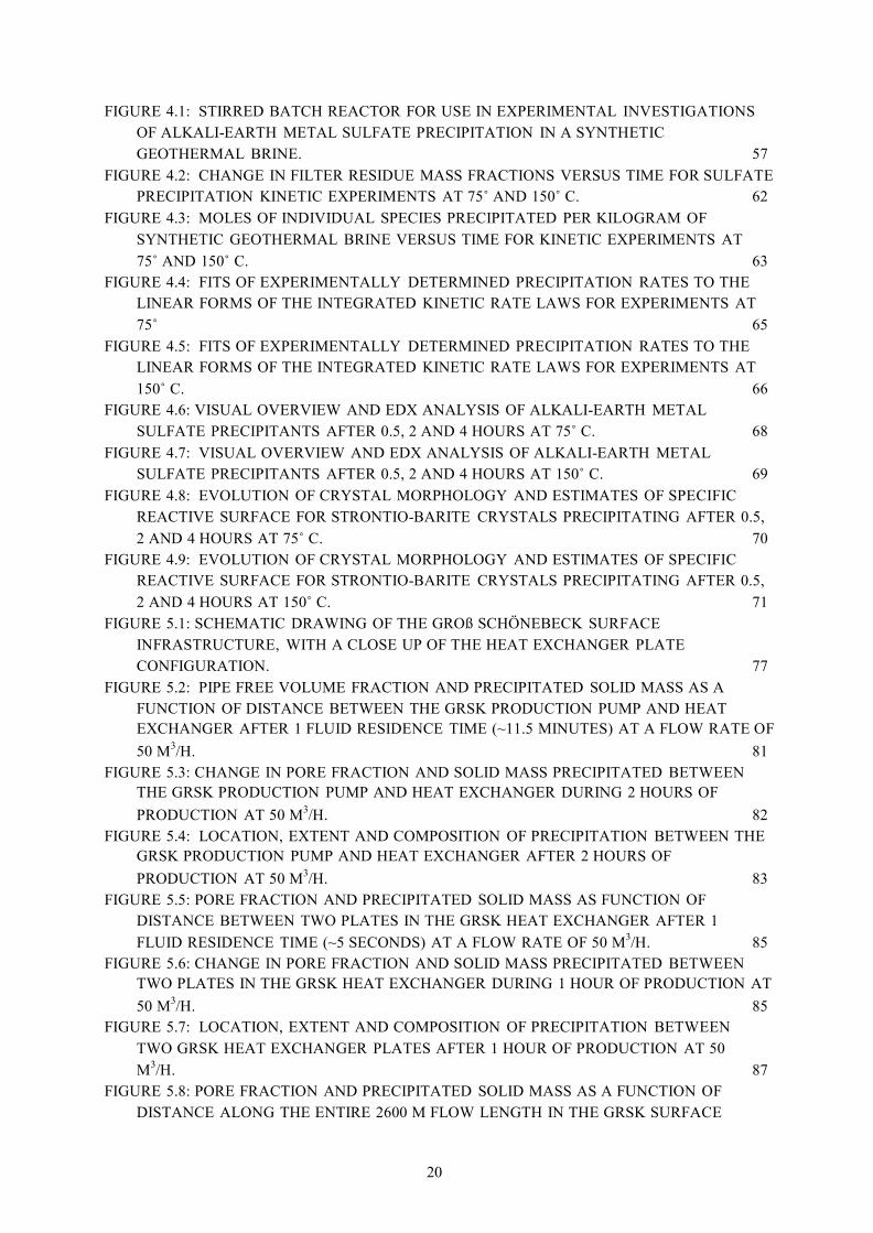
FIGURE 4.1: STIRRED BATCH REACTOR FOR USE IN EXPERIMENTAL INVESTIGATIONS OF ALKALI-EARTH METAL SULFATE PRECIPITATION IN A SYNTHETIC GEOTHERMAL BRINE. 57

FIGURE 4.2: CHANGE IN FILTER RESIDUE MASS FRACTIONS VERSUS TIME FOR SULFATE PRECIPITATION KINETIC EXPERIMENTS AT 75˚ AND 150˚ C. 62

FIGURE 4.3: MOLES OF INDIVIDUAL SPECIES PRECIPITATED PER KILOGRAM OF SYNTHETIC GEOTHERMAL BRINE VERSUS TIME FOR KINETIC EXPERIMENTS AT 75˚ AND 150˚ C. 63

FIGURE 4.4: FITS OF EXPERIMENTALLY DETERMINED PRECIPITATION RATES TO THE LINEAR FORMS OF THE INTEGRATED KINETIC RATE LAWS FOR EXPERIMENTS AT 75˚ 65

FIGURE 4.5: FITS OF EXPERIMENTALLY DETERMINED PRECIPITATION RATES TO THE LINEAR FORMS OF THE INTEGRATED KINETIC RATE LAWS FOR EXPERIMENTS AT 150˚ C. 66

FIGURE 4.6: VISUAL OVERVIEW AND EDX ANALYSIS OF ALKALI-EARTH METAL SULFATE PRECIPITANTS AFTER 0.5, 2 AND 4 HOURS AT 75˚ C. 68

FIGURE 4.7: VISUAL OVERVIEW AND EDX ANALYSIS OF ALKALI-EARTH METAL SULFATE PRECIPITANTS AFTER 0.5, 2 AND 4 HOURS AT 150˚ C. 69

FIGURE 4.8: EVOLUTION OF CRYSTAL MORPHOLOGY AND ESTIMATES OF SPECIFIC REACTIVE SURFACE FOR STRONTIO-BARITE CRYSTALS PRECIPITATING AFTER 0.5, 2 AND 4 HOURS AT 75˚ C. 70

FIGURE 4.9: EVOLUTION OF CRYSTAL MORPHOLOGY AND ESTIMATES OF SPECIFIC REACTIVE SURFACE FOR STRONTIO-BARITE CRYSTALS PRECIPITATING AFTER 0.5, 2 AND 4 HOURS AT 150˚ C. 71

FIGURE 5.1: SCHEMATIC DRAWING OF THE GROß SCHÖNEBECK SURFACE INFRASTRUCTURE, WITH A CLOSE UP OF THE HEAT EXCHANGER PLATE CONFIGURATION. 77

FIGURE 5.2: PIPE FREE VOLUME FRACTION AND PRECIPITATED SOLID MASS AS A FUNCTION OF DISTANCE BETWEEN THE GRSK PRODUCTION PUMP AND HEAT EXCHANGER AFTER 1 FLUID RESIDENCE TIME (~11.5 MINUTES) AT A FLOW RATE OF 50 M3/H. 81

FIGURE 5.3: CHANGE IN PORE FRACTION AND SOLID MASS PRECIPITATED BETWEEN THE GRSK PRODUCTION PUMP AND HEAT EXCHANGER DURING 2 HOURS OF PRODUCTION AT 50 M3/H. 82

FIGURE 5.4: LOCATION, EXTENT AND COMPOSITION OF PRECIPITATION BETWEEN THE GRSK PRODUCTION PUMP AND HEAT EXCHANGER AFTER 2 HOURS OF PRODUCTION AT 50 M3/H. 83

FIGURE 5.5: PORE FRACTION AND PRECIPITATED SOLID MASS AS FUNCTION OF DISTANCE BETWEEN TWO PLATES IN THE GRSK HEAT EXCHANGER AFTER 1 FLUID RESIDENCE TIME (~5 SECONDS) AT A FLOW RATE OF 50 M3/H. 85

FIGURE 5.6: CHANGE IN PORE FRACTION AND SOLID MASS PRECIPITATED BETWEEN TWO PLATES IN THE GRSK HEAT EXCHANGER DURING 1 HOUR OF PRODUCTION AT 50 M3/H. 85

FIGURE 5.7: LOCATION, EXTENT AND COMPOSITION OF PRECIPITATION BETWEEN TWO GRSK HEAT EXCHANGER PLATES AFTER 1 HOUR OF PRODUCTION AT 50 M3/H. 87

FIGURE 5.8: PORE FRACTION AND PRECIPITATED SOLID MASS AS A FUNCTION OF DISTANCE ALONG THE ENTIRE 2600 M FLOW LENGTH IN THE GRSK SURFACE

21

INFRASTRUCTURE AFTER 1 FLUID RESIDENCE TIME (~25 MINUTES) AT A FLOW RATE OF 50 M3/H. 88

FIGURE 5.9: CHANGE IN PORE FRACTION AND SOLID MASS PRECIPITATED ALONG THE ENTIRE 2600 M FLOW LENGTH IN THE GRSK SURFACE INFRASTRUCTURE DURING 120 HOURS (5 DAYS) OF PRODUCTION AT 50 M3/H 89

FIGURE 5.10: LOCATION, EXTENT AND COMPOSITION OF PRECIPITATION BETWEEN THE GRSK PRODUCTION PUMP AND HEAT EXCHANGER AFTER 120 HOURS (5 DAYS) OF PRODUCTION AT 50 M3/H. 90

B 1: BARITE PRECIPITATED FROM A 5 MOLAL NACL SOLUTION. 121 B 2: CELESTITE PRECIPITATED FROM A 5 MOLAL NACL SOLUTION. 122 B 3: ANHYDRITE PRECIPITATION FROM A NA-CA-CL (5 MOLAL CL) SOLUTION AFTER

0.5, 2 AND 4 HOURS. 123 B 4: STRONTIO-BARITE WITH ANHYDRITE PRECIPITATED FROM A MIXED ELECTROLYTE

(NA-CA-BA-SR-CL-SO4-H2O; 5 MOLAL CL) SOLUTION AT GRSK CONCENTRATIONS. 124

xxii

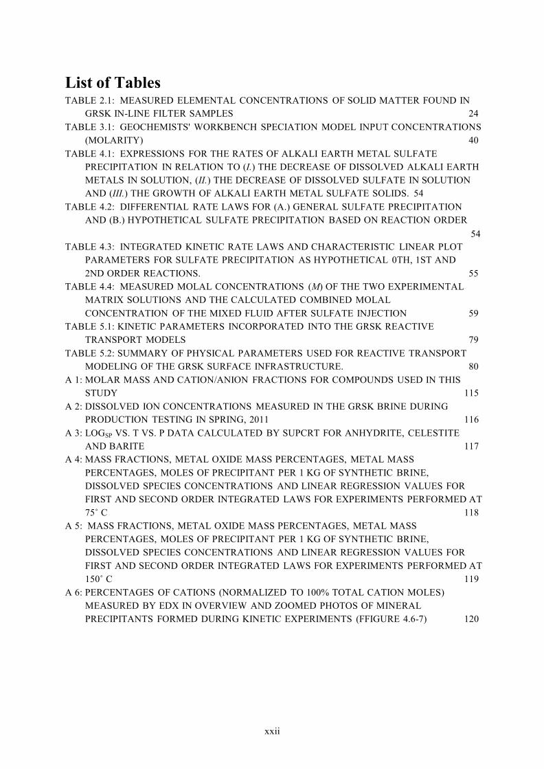
List of Tables TABLE 2.1: MEASURED ELEMENTAL CONCENTRATIONS OF SOLID MATTER FOUND IN

GRSK IN-LINE FILTER SAMPLES 24 TABLE 3.1: GEOCHEMISTS' WORKBENCH SPECIATION MODEL INPUT CONCENTRATIONS

(MOLARITY) 40 TABLE 4.1: EXPRESSIONS FOR THE RATES OF ALKALI EARTH METAL SULFATE

PRECIPITATION IN RELATION TO (I.) THE DECREASE OF DISSOLVED ALKALI EARTH METALS IN SOLUTION, (II.) THE DECREASE OF DISSOLVED SULFATE IN SOLUTION AND (III.) THE GROWTH OF ALKALI EARTH METAL SULFATE SOLIDS. 54

TABLE 4.2: DIFFERENTIAL RATE LAWS FOR (A.) GENERAL SULFATE PRECIPITATION AND (B.) HYPOTHETICAL SULFATE PRECIPITATION BASED ON REACTION ORDER

54 TABLE 4.3: INTEGRATED KINETIC RATE LAWS AND CHARACTERISTIC LINEAR PLOT

PARAMETERS FOR SULFATE PRECIPITATION AS HYPOTHETICAL 0TH, 1ST AND 2ND ORDER REACTIONS. 55

TABLE 4.4: MEASURED MOLAL CONCENTRATIONS (M) OF THE TWO EXPERIMENTAL MATRIX SOLUTIONS AND THE CALCULATED COMBINED MOLAL CONCENTRATION OF THE MIXED FLUID AFTER SULFATE INJECTION 59

TABLE 5.1: KINETIC PARAMETERS INCORPORATED INTO THE GRSK REACTIVE TRANSPORT MODELS 79

TABLE 5.2: SUMMARY OF PHYSICAL PARAMETERS USED FOR REACTIVE TRANSPORT MODELING OF THE GRSK SURFACE INFRASTRUCTURE. 80

A 1: MOLAR MASS AND CATION/ANION FRACTIONS FOR COMPOUNDS USED IN THIS STUDY 115

A 2: DISSOLVED ION CONCENTRATIONS MEASURED IN THE GRSK BRINE DURING PRODUCTION TESTING IN SPRING, 2011 116

A 3: LOGSP VS. T VS. P DATA CALCULATED BY SUPCRT FOR ANHYDRITE, CELESTITE AND BARITE 117

A 4: MASS FRACTIONS, METAL OXIDE MASS PERCENTAGES, METAL MASS PERCENTAGES, MOLES OF PRECIPITANT PER 1 KG OF SYNTHETIC BRINE, DISSOLVED SPECIES CONCENTRATIONS AND LINEAR REGRESSION VALUES FOR FIRST AND SECOND ORDER INTEGRATED LAWS FOR EXPERIMENTS PERFORMED AT 75˚ C 118

A 5: MASS FRACTIONS, METAL OXIDE MASS PERCENTAGES, METAL MASS PERCENTAGES, MOLES OF PRECIPITANT PER 1 KG OF SYNTHETIC BRINE, DISSOLVED SPECIES CONCENTRATIONS AND LINEAR REGRESSION VALUES FOR FIRST AND SECOND ORDER INTEGRATED LAWS FOR EXPERIMENTS PERFORMED AT 150˚ C 119

A 6: PERCENTAGES OF CATIONS (NORMALIZED TO 100% TOTAL CATION MOLES) MEASURED BY EDX IN OVERVIEW AND ZOOMED PHOTOS OF MINERAL PRECIPITANTS FORMED DURING KINETIC EXPERIMENTS (FFIGURE 4.6-7) 120

23

List of Abbreviations and Symbols (T, p, x): Temperature, pressure and composition

[A]x: Generic expression for an xth order kinetic reaction

˚ C: Degrees Celsius

α: Activity of a species

A: Empirically fitted parameter for the Debye-Hückel equation

Ao: Parameter describing the average distance between two ions in the Debye-

Hückel equation

B: Empirically fitted parameter for the Debye-Hückel equation

BaSO4: Barite

CA: Cellulose Acetate (filter)

CaCO3: Calcite

CaSO4: Anhydrite

CEBS: Central European Basin System

cm: 10-2 meters

Cu2CO3[OH]: Malachite

ΔGr˚: Standard state Gibbs’ energy of a reaction

EDX: Energy dispersive x-ray spectroscopy

EGS: Enhanced geothermal system

FluMo: Online fluid monitoring system at GrSk

γ: Activity coefficient

g/cm3: Grams per cubic centimeter (units for density)

g/m3: Grams per cubic meter of produced brine (units for precipitated mass)

GrSk: Groß Schönebeck in-situ geothermal laboratory

GrSk 3/90: Injection well at GrSk

GrSk 04/05: Production well at GrSk

GW: Gigawatt

GWB: Geochemists’ Workbench

I: Ionic strength

IAP: Ion activity product

IC: Ion chromatograph

ICP-OES: Inductively coupled plasma optical emissions spectrometry

k: kinetic reaction rate coefficient

kg: 103 grams

kg of brine•mm-1•s-1: Kilogram of brine per millimole second (units for second order kinetic

reaction)

24

Ksp: Thermodynamic equilibrium constant

l•mg-1•h-1: Liters per milligram hour (units for second order kinetic reaction)

m: Meter (regular script distinguishing from molality)

M: Molarity

m: Molality (cursive script distinguishing from meters)

m2: Square meters

m3: Cubic meters

ml: 10-3 liters

mM: 10-3 molar

mm: 10-3 molal

MPa: 106 pascals (pressure)

NaCl: Halite

NEGB: Northeast German Basin

ORC: Organic Rankine Cycle

PbCl[OH]: Laurionite

PEEK: Polyetheretherketone (plastic)

PFA: Perfluoroalkoxy (plastic)

PTFE: Polytetrafluoroethylene (plastic; Teflon)

QNT: Qunitessa® Pitzer database

r: Radius of a sphere

SA: Surface area of a solid

SEM: Scanning electron microscope

SI: Saturation index

SrSO4: Celestite

SS-304: 304-grade stainless steel

SS-316: 316-grade stainless steel

SSA: Specific reactive surface area of a solid

TDS: Total dissolved solids

TWh/y: Terawatt hour per year

V: Volume of a solid

XRD: X-ray diffraction

XRF: X-ray fluorescence

z: Charge of a dissolved ion

λ: Empirically determined Pitzer parameter for the 2nd virial expansion

µ: Empirically determined Pitzer parameter for the 3rd virial expansion

µm: 10-6 meters

µM: 10-6 molar

1

1. Introduction

2

1.1 Geothermics as viable renewable energy in the 21st

century Geothermics are an essential part of a mix of renewable resources designed to produce clean energy in

the 21st century. Although solar and wind power are often cited as the driving force behind the growth

of renewable energies, geothermal resources within the uppermost 10 km of the Earth’s crust contain

three times as much energy as insolation and eight times as much energy as global wind reserves

(Sims et al., 2007; MIT, 2006). Nonetheless, the capitalization of geothermal energy as a renewable

alternative to fossil fuels has been relatively slow compared to solar and wind power.

The slow growth of geothermal energy production compared to other renewable resources may be due

to the large gap between known geothermal reserves and the technical know-how to recover them

(Jacobson, 2009). Conventional geothermal energy is produced in volcanically or tectonically active

areas, where the geothermal gradient is anomalously high. In these locations, the elevated incidence of

faulting and fracturing in the subsurface allows for unimpeded migration of thermal fluids to shallow

depths and favorable hydraulic conditions for fluid production in the reservoir, respectively (U.S.

D.O.E., 2008; MIT, 2006; Muffler, 1993; Muffler, 1978). Such systems have been used successfully

for centuries as direct-use heat sources and for nearly 100 years as a commercial-grade electricity

source (Dixon and Fannelli, 2003; Cataldi et al., 1999).

Globally significant utilization of geothermal energy necessitates the harvesting of heat from non-

conventional resources found in places of ordinary geothermal gradients and where there may be little

to no subsurface geothermal fluid flow. Such heat reservoirs require substantial engineering and

stimulation before their heat energy can be obtained. Reservoirs that have been specifically

engineered for heat extraction from the subsurface are known as ”enhanced geothermal systems”

(EGS), and they show great potential for bringing geothermics onto the main stage of global energy

production (Sullivan et al., 2010; MIT, 2006). Recent developments in the drilling and production

technology required for commercially feasible EGS utilization have allowed geothermal energy

production to expand beyond its traditional limits defined by geological settings. Consequently, global

installed capacity (in GW) and production (in TWh/y) of geothermal-based electricity has increased by

nearly 40% in the first decade of the 21st century, to ~11 GW and ~67 TWh/y, respectively (Bertani,

2012). Currently, 24 countries around the world are producing electricity from geothermal sources

(Bertani, 2012). Geothermal energy is used directly (e.g. heating/cooling, balynology, industrial

drying) by a total of 78 countries on six different continents (Lund, 2010). The global installed

capacity of geothermal energy is expected to nearly double by 2015 (Bertani, 2012). The energy

requirements of 750,000,000 million people worldwide, including 100% of the residents of 39

different countries, can potentially be met by geothermal resources (Gawell et al., 1999).

3

Sedimentary basins, in particular, have received considerable attention as potential geothermal

resources (e.g. Norden et al., 2009, Hartmann et al., 2008; Manning et al., 2007; Erdlac et al. 2007;

Blackwell et al., 2007; MIT, 2006; Reyes and Jongens, 2005; Genter et al., 2003; Jessop and

Majorowicz, 1994; Majorowicz and Jessop, 1981; Muffler, 1978; Jones, 1970; Helgeson, 1968). They

are widespread across the globe and underlie many of the world’s major population centers. Even

under normal geothermal gradients (i.e. ~ 30° C per kilometer depth), in-situ formation fluids in

sedimentary basins can be produced for direct heating use from depths of less than 2 km (Huenges et

al., 2010). Recent advances in binary plant processes, which transfer heat from the geothermal fluid to

a low-boiling point working fluid that is then fed to a turbine, also render electricity production from

formation fluids found at depths of less than 5 km technologically feasible (Frick et al., 2010; Heberle

and Brüggermann, 2010; Franco and Villani, 2009; Hettiarachchi et al., 2007; DiPippo, 2004). Wells

drilled to such depths are commonplace in the oil and gas industry and can be constructed with

currently available drilling technology. Adapting existing technology to the production and re-

injection of formation fluids is currently a central focus of the EGS community and an essential step

towards realizing the full potential of geothermal energy.

1.2 The Groß Schönebeck in-situ Geothermal Laboratory

A network of sedimentary basins such as those described above is spread across Northern and Central

Europe in the Central European Basin System (CEBS), a sketch of which is found in Figure 1.1. The

origin, evolution and modern dynamics of the sub-basins within this network have been extensively

studied by many researchers (e.g. Maystrenko et al., 2012; Noack et al., 2010; Moeck et al., 2009;

Menning et al., 2006; Kaiser et al., 2005; Littke et al., 2005; Lüders et al., 2005; Scheck-Wenderoth

and Lamarch, 2005; Wilson et al., 2004; van Wees et al., 2000; Bayer et al., 1999; Breitkreuz and

Kennedy, 1999; Scheck and Bayer, 1999; Bayer et al., 1997; Thybo, 1997; Benek et al., 1996;

Coward, 1995; Dadlez et al., 1995; Glennie, 1995; Brink et al., 1992). The individual basins within

the CEBS are representative of sedimentary basins around the world and are, therefore, prime targets

for EGS exploration and development. With temperatures greater than 150˚ C at depths of less than 5

km (e.g. Noack et al., 2010; Ollinger et al., 2010; Norden et al., 2008; Norden and Förster, 2006;

Förster 2001, Cermak, 1993), the subsurface thermal regime in the Permo-carboniferous Northeast

German Basin (NEGB; Figure 1.1) makes this a particularly promising area for EGS growth.

4

GrSK

Berlin

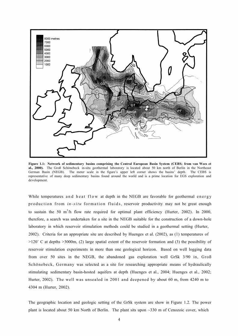
Figure 1.1: Network of sedimentary basins comprising the Central European Basin System (CEBS; from van Wees et al., 2000). The Groß Schönebeck in-situ geothermal laboratory is located about 50 km north of Berlin in the Northeast German Basin (NEGB). The meter scale in the figure’s upper left corner shows the basins’ depth. The CEBS is representative of many deep sedimentary basins found around the world and is a prime location for EGS exploration and development.

While temperatures a n d h e a t f l o w at depth in the NEGB are favorable for geothermal e n e r g y

p r oduc t i on f r om in - s i t u fo r m a t i o n f l u i d s , reservoir productivity may not be great enough

to sustain the 50 m3/h flow rate required for optimal plant efficiency (Hurter, 2002). In 2000,

therefore, a search was undertaken for a site in the NEGB suitable for the construction of a down-hole

laboratory in which reservoir stimulation methods could be studied in a geothermal setting (Hurter,

2002). Criteria for an appropriate site are described by Huenges et al. (2002), as (1) temperatures of

>120˚ C at depths >3000m, (2) large spatial extent of the reservoir formation and (3) the possibility of

reservoir stimulation experiments in more than one geological horizon. Based on well logging data

from over 50 sites in the NEGB, the abandoned gas exploration well GrSk 3/90 in , G r o ß

Sc h ö n e be c k, G e r m a ny was selected as a site for researching appropriate means of hydraulically

stimulating sedimentary basin-hosted aquifers at depth (Huenges et al., 2004; Huenges et al., 2002;

Hurter, 2002). Th e w e l l w a s u n s e a l e d i n 2 0 0 1 a n d d e e p e n e d b y about 60 m, from 4240 m to

4304 m (Hurter, 2002).

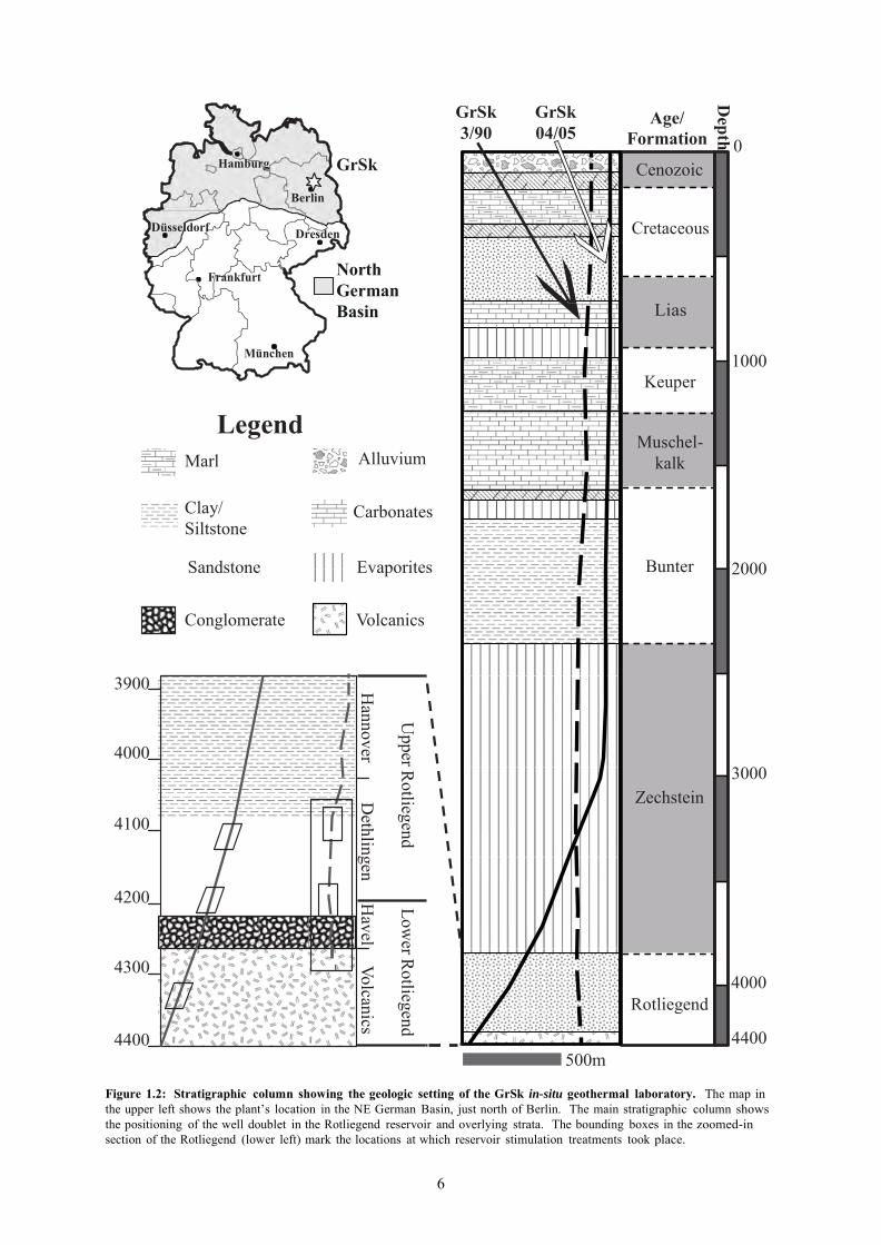
The geographic location and geologic setting of the GrSk system are show in Figure 1.2. The power

plant is located about 50 km North of Berlin. The plant sits upon ~330 m of Cenozoic cover, which

5

overlies ~2037 m of lithified Mesozoic sediments, consisting of (from youngest to oldest) the

Cretaceous, Lias, Keuper, Muschelkalk and Bunter formations (Lenz et al, 2002). Beneath the

Mesozoic section lies nearly 1500 m of the Permian Zechstein evaporate deposits (Huenges et al.,

2004). The Zechstein is underlain by the Permian Rotliegend formation, which, at this location

consists of ~400 m of siliciclastic sedimentary rocks, underlain by ~60 m of andesitic extrusive rocks

(Huenges et al, 2007; Huenges et al., 2004). The geothermal reservoir at GrSk is located in the

Rotliegend Formation. A well doublet, consisting of a production well (GrSk 4/05) and an injection

well (GrSk 3/90), terminate within the volcanic section of the Rotliegend Formation at depths of

~4300 – 4400 m (Frick et al., 2011; Huenges et al., 2004). Temperature and pressure conditions in

the reservoir are ~150˚ C and 45 MPa, respectively (Frick et al., 2011).

Hydraulic testing performed after re-opening the GrSk 3/90 well produced roughly 335 m3 of

geothermal brine at a flow rate of 7-11 m3/hr. Three gas and condensed fluid samples were taken from

a depth of 4200 m concurrent to this initial production, revealing the formation water to be a Ca-Na-Cl

type brine typical of Rotliegend formation waters (Wolfgramm et al., 2004; Holl et al., 2003; Giese et

al, 2002). Detailed discussions of the GrSk brine’s chemistry are found in Chapters 2 & 3 of this

work. The initial production testing was followed by 2 fracturing treatments (Holl et al., 2003; Giese et al.,

2002). The locations of these treatments in the reservoir are shown in Figure 1.2. The first treatment

was performed using conventional methods in two separate horizons of the Elbe subgroup of the

Lower Permian Rotliegend (Zimmerman et al., 2005; Huenges et al., 2004; Tischner et al, 2004). The

upper treatment was located at the boundary between the Hannover and Dethlingen formations (~4080

m to 4120 m), while the lower treatment took place at the lower boundary of the Dethlingen (4130 m

to 4190 m), above the basal conglomerates of the Havel Formation (Zimmerman et al., 2005; Huenges

et al., 2004; Tischner et al, 2004). The second treatment was performed throughout the entire open-

hole section of the well, beginning at 3874 m and terminating in the volcanic section at the bottom of

the well (4294 m; Zimmerman et al., 2005; Huenges et al., 2004; Tischner et al, 2004). This treatment

involved the development and application of techniques beyond those commonly employed in the oil

and gas industry (Legarth et al., 2005; Reinicke et al., 2005).

The successful treatments increased reservoir productivity to 25 m3/h (Holl, et al., 2003). Subsequent

to the post-stimulation productivity test, a low production level of ~ 1 m3/hr was maintained for a few weeks (Holl et al., 2003).

6

Depth

Upper R

otliegend Low

er Rotliegend

Hannover

Dethlingen

Havel

Volcanics

Hamburg

Berlin

GrSk

GrSk 3/90

GrSk 04/05

Age/ Formation 0

Cenozoic

Düsseldorf

Frankfurt

Dresden

North German Basin

Cretaceous

Lias

München

Legend

Marl Alluvium

Keuper

Muschel- kalk

1000

Clay/ Siltstone

Carbonates

Sandstone Evaporites Bunter 2000

Conglomerate Volcanics

3900

4000

4100

4200

Zechstein

3000

4300

4400

500m

Rotliegend

4000

4400

Figure 1.2: Stratigraphic column showing the geologic setting of the GrSk in-situ geothermal laboratory. The map in the upper left shows the plant’s location in the NE German Basin, just north of Berlin. The main stratigraphic column shows the positioning of the well doublet in the Rotliegend reservoir and overlying strata. The bounding boxes in the zoomed-in section of the Rotliegend (lower left) mark the locations at which reservoir stimulation treatments took place.

7

After the production of about 700 m3 of fluid, the pump was removed, revealing the accumulation of

laurionite (PbCl[OH]), malachite (Cu2[CO3][OH]), native lead and barite (BaSO4) precipitants in the

pump, well casing and cables (Holl et al., 2003). A bailer sample taken at depth also revealed

authigenic native copper, native lead, calcite (CaCO3) and barite precipitation (Holl, et al., 2003). The

accumulation of these mineral precipitants during the start up of the GrSk project raises serious

questions as to how mineral precipitation within the plant’s infrastructure may impact regular plant

operations. The purpose of this work, therefore, is to characterize the nature and extent of this mineral

precipitation, i.e. scaling (see section 1.3 below). The GrSk 3/90 well now serves as the injection well

in the GrSk plant.

To complete the well doublet system, a second well (GrSk 4/05) was drilled to serve as a production

well (Huenges et al., 2007; Zimmerman et al., 2007). This well reaches a depth of 4400m and is

deviated 47° in the direction of the minimum horizontal stress in reservoir (Figure 1.2), separating the

two wells at depth by about 500 m (Huenges et al, 2007; Zimmerman et al., 2007). The deviated well

creates additional space in the subsurface between the wells, preventing cold re-injected water from

quickly reaching the production well (Zimmerman et al., 2007). The well’s deviation also enhances the

hydraulic fracturing treatments by aligning stresses created by stimulation parallel to the direction of

maximum stress in the reservoir (Huenges et al, 2007). Hydraulic fracturing treatments were

performed in 2 horizons of the Dethlingen Sandstone Formation of the Upper Rotliegend, and one

treatment was performed in the volcanic section of the Lower Rotliegend (Figure 1.2; Zimmerman et

al., 2008). Both of these stimulations took place in perforated sections of the well (Zimmermann et

al., 2008). The combined stimulation treatments enabled a productivity of ~30 m3/hr., a 500%

increase over the untreated reservoir (Zimmermann et al., 2010).

The success of the drilling and reservoir stimulation operations at GrSk allowed the project’s research

activities to expand into many different areas. In addition to adapting directional drilling and reservoir

stimulation methods to geothermal systems, the GrSk in-situ laboratory is also equipped to research

geothermal exploration methods, geothermal reservoir engineering methods, turbine technology,

power plant performance optimization, fluid chemistry throughout the brine’s circulation path,

material corrosion in contact with geothermal brine and testing of individual components in a power or

co-generation plant (Saadat et al., 2010). To facilitate this research, a geothermal plant surface

infrastructure is under construction. The finished plant will include a heat exchanger, research ORC,

cooling tower, production and injection pumps, electronic automation of all systems and a completed

geothermal fluid loop (reservoir – production – heat transfer – injection – reservoir) (Kranz et al.,

2010). Of particular relevance to the investigation of chemical challenges in the geothermal industry

is the inclusion of a fluid monitoring bypass (FluMo) that allows the online monitoring of a variety of

physico- and electrochemical parameters, such as temperature, pressure, volumetric flow rate, pH,

8

redox potential and electrical conductivity (Regenspurg et al., 2012; Milsch et al., 2010). A detailed

discussion of the GrSk brine’s chemical composition is found in Chapter 2, below.

1.3 Scaling

Due to their great age and, therefore, extensive interaction with surrounding rock formations, high

ionic strength (especially from dissolved chloride salts) is a common feature of formation fluids found

in deep sedimentary basins (e.g. Frape et al., 2004; Kharaka and Hanor, 2004; Kuhn et al., 2003; Bazin

and Brosse, 1997; D’amore, et al., 1997; Hanor, 1994; Baccar et al., 1993; Fontes and Matray, 1993;

Pauwels et al., 1993; Platt, 1993; Williams and McKibben 1989; Kharaka et al., 1985; Eugster and

Jones, 1979). Elevated concentrations of dissolved mineral species in such brines, combined with

abrupt changes in (T, p, x) conditions along the geothermal loop, create a scaling risk during plant

operation. Scaling, or process fouling by mineral growth on an industrial infrastructure, is a well-

known hazard in many industries and has recently been the focus of much research in the geothermal

community (e.g. Frick et al., 2011; Minissale et al., 2008; Yanagisawa et al., 2008; Wilson et al., 2007;

Gunarsson and Arnorsson, 2005; Yanagisawa et al., 2005; Kuhn et al., 2003, Reyes et al., 2002;

Criaud and Fouillac, 1989; Thomas and Gudmundsson, 1989). Such scaling can reduce pipe diameters

and create a coating on the heat exchanger units, thereby reducing the plant’s productivity and thermal

transfer efficiency, respectively (Gunarsson and Arnorsson, 2005). Certain types of mineral scales can

also cause or accelerate corrosion in the plant’s infrastructure (e.g. Refait et al., 2006; Valencia-

Cantero et al., 2003) All of these circumstances are obstacles to the long-term operational and

financial stability of a geothermal heat or power plant.

The formation of mineral scales is dependent on various physical, electrochemical, thermodynamic

and microbiological factors. On the most fundamental level, whether or a not mineral will precipitate

from solution is a function its saturation index (SI), a property defined by the quotient of the ion

activity product (IAP) of the mineral’s components and the mineral’s thermodynamic equilibrium

constant (Ksp) (Drever, 2002). A detailed discussion of ion activity determinations in saline solutions

is found in Chapter 3 of this work. If the IAP of a mineral’s components is greater than its Ksp, the

mineral is considered oversaturated and may precipitate to bring superfluous ions out of solution in a

solid form (Drever, 2002). Equilibrium constants are temperature and pressure dependent; changes in

a solution’s temperature and pressure conditions may move a mineral from an undersaturated to an

oversaturated state, or vice versa, even if the ionic concentrations remain constant (Drever, 2002).

Variations in a mineral’s saturation index are, therefore, an avoidable consequence of any heat

exchange process. In a similar manner, ion activities are also temperature and pressure dependent and

are predestined to be altered during plant operation. Furthermore, electrochemical factors such as pH

and redox potential may also influence a mineral’s solubility in aqueous solutions (Drever, 2002).

9

Finally, even if a mineral is deemed oversaturated, or if the electrochemical condition of the fluid

favors a mineral’s precipitation, the rate of the precipitation reaction may be slow enough to prevent

the mineral from precipitating within the time frame of the production/reinjection cycle (e.g. Fritz and

Noguera, 2009; Hsu 2006; Gunarsson, et al., 2005; Ganor et al., 2004; Martin and Lowell, 2000;

Caroll et al. 1998; Devidal et al., 1997; Gislason et al., 1997; Grundl and Delwiche, 1993; Nagy and

Lasaga, 1992;Mullis, 1991; Nagy et al., 1991; Murphy and Helgeson, 1989; Bird, et al., 1986;

Atkinson et al., 1977). Therefore, knowledge of precipitation reaction kinetics is also required in order

to understand the phenomenon of scaling.

Several geochemical modeling software packages, such as PHREEQc (Parkhurst, 1995), WATEQ4F

(Ball and Nordstrom, 1991), MINETQA2/PRODEFA2 (Allison et al, 1991) and SOLMINEQ.88

(Kharaka et al, 1988), exist to facilitate predictions of scaling risks, both in terms of identifying

oversaturated phases and quantifying the specific mass of precipitant that will return the solution to

thermodynamic equilibrium. More comprehensive programs, such as the Geochemist’s Workbench

(Bethke, 2008), or TOUGHREACT (Xu et al., 2005), also allow for the integration of kinetic rate laws

into multi-dimensional reactive transport models. Equilibrium models of the GrSk brine at conditions

found in the GrSk surface installation (75˚-150˚ C, 0.1 MPa) and in the reservoir (150˚ C, 45 MPa) are

found in Chapter 3 of this work.

1.4 Goals of present study

Scaling is a fundamental geochemical hazard expected during the operation of the GrSk in-situ

geothermal laboratory (Frick et al., 2011; Regenspurg et al., 2010, Holl et al., 2003, Seibt and

Wolframm, 2003, Giese, et al., 2002). In their initial study of the GrSk fluid, Giese et al. (2002)

identified several potentially oversaturated phases in the brine with the modeling program

SOLMINEQ.88 (Kharaka et al., 1988). Holl et al., (2003) first described the occurrence of scaling on

the pump, well casing and cables after the initial stimulation and testing in well GrSk 3/90. Based on

preliminary geochemical modeling, Regenspurg, et al., (2010) discuss the likelihood of scaling

amongst carbonate, sulfate and oxide minerals. Sulfate minerals, in particular, are well-known scale-

forming minerals in oil and gas fields (e.g. BinMerdah et al., 2009; Shen et al., 2009; BinMerdah and

Yassin, 2007; Tomson et al., 2005; He et al., 1994; Yuan et al., 1993; Gardner and Nancollas, 1983).

Because the GrSk 3/90 well was initially drilled for gas exploration, it stands to reason that sulfate

minerals may also present a risk to the geothermal plant at this site. Barite scale, for example, has

already been identified in the GrSk infrastructure (Regenspurg, et al., 2010, Holl, et al., 2003, Seibt

and Wolframm, 2003). Therefore, based on (1) modeled results, (2) field evidence from this work and

previous studies and (3) reports from the literature, sulfate scaling has been identified as a primary

10

scaling hazard in the GrSk system. Quantifying the extent of sulfate mineral precipitation in the GrSk

plant during regular plant operation is the goal of the research presented in this work.

A flow chart documenting the scaling-risk assessment procedure performed during this study for the

GrSk site is found in Figure 1.3. An interdisciplinary approach, combining field studies, geochemical

modeling and experimental geochemistry, is employed in pursuit of the above-mentioned goal. An

important secondary goal of this research is that the procedure developed to predict scaling risks in the

GrSk system be applicable to risk assessment in a variety of geothermal systems, especially systems

producing formation waters from deep sedimentary basins. The assessment methodology is, therefore,

laid out in a step-by-step fashion.

Field Work

• Determination system

composition

Equilibrium Model

• Speciation of

brine and identification of

potentiallly oversaturated

phases

Reaction Kinetics

• Experimental derivation of

precipitation rate laws

Predictive Model

• Incorporation of

rate laws into predictive model

Figure 1.3: Flow chart depicting the process for evaluating scaling risks in geothermal systems. The method is applied in this work to a case study of sulfate mineral scaling risks in the GrSk plant, Germany

Initial field studies of the GrSk site are presented in Chapter 2. The chemical composition of brine

sampled during production testing is measured and compared with the data from Giese (2002). Fluid

is sampled and prepared under anoxic conditions. Cation concentrations are measured with

inductively coupled plasma optical emissions spectrography (ICP-OES), and anion concentrations are

measured with an ion-chromatograph (IC). The mass fraction of advectively transported solids within

the brine is calculated as a function of temperature. The composition and mineralogy of the solids in

the plant’s filtration system are determined with XRF and XRD analyses, respectively.

Chapter 3 uses the chemical data presented in Chapter 2 to derive equilibrium thermodynamic and

reaction path models of the GrSk brine as it travels the plant’s geothermal loop (reservoir-production-

heat transfer-injection-reservoir). Activity coefficient determinations in high ionic strength fluids are

discussed, along with the relative merits of existing Pitzer databases when applied to the GrSk system.

Calculated ion activities within the Na-Ca-Ba-Sr-Cl-SO4-H2O system are incorporated into reaction

path models describing the system from the time it enters the production well to the time it leaves the

11

injection well. Due to (1) the questionable reliability of existing Pitzer parameters at GrSk conditions

and (2) lack of kinetic parameters in the reaction path model, the results of this chapter are taken as

guidelines, rather than predictions.

A corrosion-resistant batch reaction system for determining mineral solubilities and reaction kinetics

in geothermal brines is presented in Chapter 4. The method developed therein is engaged in

determining alkali-earth metal sulfate precipitation rate laws from a mixed electrolyte (Na-Ca-Sr-Ba-

Cl-SO4-H2O) solution. The method of integrated rates is used, and the precipitation rate is determined

by measuring the solid weight fraction sampled from the autoclave at discrete time intervals over 4

hours. Chemical analysis of the filter residue is performed via XRF. The chemical analysis allows the

measured mass fractions to be converted into specific molal concentrations. Rate laws are then

determined by fitting the molal change in a chemical species over time to the linear plot characteristic

of an integrated rate equation for a specific reaction order. Once the reaction order is known, the rate

coefficient can be directly determined from the slope of the best-fit line. Solid phase identification and

the semi-quantitative change in the solid phases’ reactive surface areas over time are determined with

a scanning electron microscope (SEM). Chapter 5 incorporates the precipitation rate laws calculated in Chapter 4 into a predictive model of

scaling risks in the GrSk surface infrastructure. Three different models are constructed, representing

flow through 3 different sections of the GrSk surface infrastructure. Although the concentrations of

reactive species used in the Chapter 4 kinetic experiments are deliberately higher than the measured

GrSk concentrations, the rate laws are made relevant to the GrSk system by incorporating the field

data discussed in Chapter 2 into the rate laws determined in Chapter 4. Thus, the model takes into

account the concentration dependency of the precipitation rate and is directly applicable to the GrSk

system, despite the difference between the concentrations of the experimental fluids and the real GrSk

brine. In summary, the overarching goal of this work is to predict sulfate mineral scaling risks in the GrSk

surface infrastructure. The procedures used to facilitate this prediction should be applicable to brines

other than that found at GrSk. The work presents a methodology for quantifying scaling risks, and the

method is applied in a predictive manner to the GrSk brine. Intermediary goals leading to the reliable,

quantitative prediction of sulfate scaling risks in the GrSk system are:

1. To constrain the composition of the GrSk brine, apart from the influence of fluids injected

during stimulation treatments, by using field data newly obtained during production testing in

comparison with previously performed chemical analysis of the GrSk brine

2. To model the equilibrium state of the Na-Ca-Sr-Ba-Cl-SO4-H2O subsystem of the GrSk brine

throughout the geothermal loop

12

3. To determining kinetic rate laws for alkali earth metal sulfate precipitation from a synthetic

geothermal brine.

4. To incorporate the rate laws obtained in #3, above, into a 1-D reactive transport model

predicting scaling risk posed by alkali earth metal sulfates in the GrSk surface infrastructure.

13

2. Characterization of solid and liquid phases sampled during production testing

at the Groß Schönebeck in-situ

geothermal laboratory

14

2.1 Introduction In the spring of 2011, fluid production tests were performed at GrSk. In an effort to (1) further

constrain the chemical composition of the GrSk brine, (2) estimate the mass of solid material

transported within the fluid during production and (3) determine the chemical and mineralogical

composition of the solid phases, fluid and solid phase samples were collected. To reduce the effects of

fluid, gels and proppants injected into the reservoir during the stimulation treatments described in the

introduction to this work, fluid sampling commenced after 2000 m3 of fluid was produced. Sampled

fluid was analyzed for cation, anion and total dissolved carbon concentrations. The mass fraction of

advectively transported solids within the brine was determined by filtering a small amount (~10-20 ml)

of brine through a syringe filter and dividing the mass of filter residue by the total mass of the sampled

system (filter residue + sampled fluid). Solid samples were taken from the plant’s in-line filters for

determination of the filter residue’s chemical composition and mineralogy with XRF, XRD, and SEM.

2.2 Methods

2.2.1 Fluid sampling

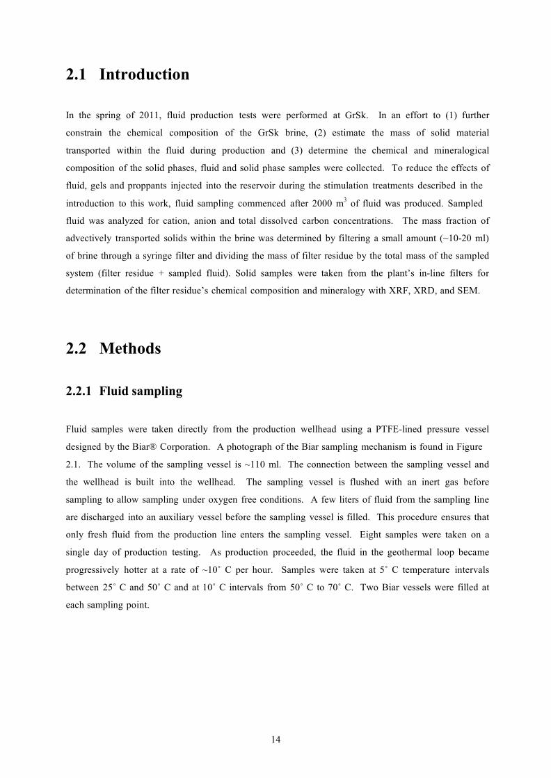
Fluid samples were taken directly from the production wellhead using a PTFE-lined pressure vessel

designed by the Biar® Corporation. A photograph of the Biar sampling mechanism is found in Figure

2.1. The volume of the sampling vessel is ~110 ml. The connection between the sampling vessel and

the wellhead is built into the wellhead. The sampling vessel is flushed with an inert gas before

sampling to allow sampling under oxygen free conditions. A few liters of fluid from the sampling line

are discharged into an auxiliary vessel before the sampling vessel is filled. This procedure ensures that

only fresh fluid from the production line enters the sampling vessel. Eight samples were taken on a

single day of production testing. As production proceeded, the fluid in the geothermal loop became

progressively hotter at a rate of ~10˚ C per hour. Samples were taken at 5˚ C temperature intervals

between 25˚ C and 50˚ C and at 10˚ C intervals from 50˚ C to 70˚ C. Two Biar vessels were filled at

each sampling point.

15

Figure 2.1: Biar system for sampling corrosive fluids from the geothermal production line under oxygen-free conditions. The PTFE-lined, 110 mL sampling vessel (left) is flushed with nitrogen to remove all oxygen from the chamber before being connected to the sampling valve located directly on the production wellhead (right).

2.2.2 Fluid Preparation

Once full, the sampling vessel is inserted into a nitrogen (N2) filled glove box (O2 atmosphere < 0.1

ppm). The fluid from one sampling vessel is released from the vessel into a glass beaker and divided

into three parts. The first part is acidified to pH < 2 with 6 M nitric acid and set aside for cation

analysis. The second part is diluted 1000:1 with distilled water and set aside for anion analysis. PTFE

bottles are filled with 30 ml of both cation and anion samples and wrapped in Parafilm® before being

removed from the glovebox and sent to the laboratory for analysis. The third part of the fluid from the

first vessel is filled into a syringe and filtered through a pre-weighed, 0.2 µm cellulose acetate (CA)

filter into PTFE beaker of known mass. The beaker with the filtered fluid is weighed, and the mass of

sampled fluid is calculated as the difference in mass between the empty beaker and the beaker plus the

filtered fluid. The mass of the filtered fluid is used to determine the mass fraction of precipitant in the

brine, as discussed in Section 2.2.4, below. Fluid contained in the second Biar sampling vessel is

emptied into a PTFE bottle, wrapped with parafilm and sent to the laboratory for total dissolved

carbon determination.

16

2.2.3 Solid phase sampling and preparation The CA filter used in filtering the sampled fluid is flushed profusely with distilled water to remove any

soluble phases and is left overnight at 105˚ C in a drying oven. The filter plus the dried filter residue

is weighed, and the difference in mass between the unused filter and the filter plus dried filter residue

is the mass of the filter residue. Solid samples are also collected from the filtration system built into

the plant’s production line. Pictures of the filters used in the GrSk plant and the filter residue contained

within a used filter are found in Figure 2.2. Produced fluid is filtered through a 10 µm and a 2 µm

filter before entering the heat transfer section of the geothermal loop. Approximately 5x5 cm square

pieces material are cut out of the used filters of both sizes and dried overnight at 105˚ C. Dried filter

residue is separated from the filter and ground with a mortar and pestle. Two hundred milligrams of

the dried, powdered filter residue are formed into glass disks for x-ray fluorescence (XRF)

determination of the filter residue’s chemistry. A small portion of the leftover filter residue is

sprinkled onto scanning electron microscope (SEM) slides. The remaining filter residue is packed into

XRD cartridges for determination of the solid phase mineralogy. Photographs of some samples

prepared for XRF and XRD analyses are found in Figure 2.3.

Figure 2.2: Filter bags (left) and close-up of filter residue (right) from the GrSk in-line filtration system. Filters with pore sizes of 10 µm and 2 µm remove suspended solids from the brine before it enters the heat transfer section of the geothermal loop

2.2.4 Sample Analysis

The VKTA laboratory in Dresden, Germany determined the chemical compositions of fluid samples

from this study. This accredited laboratory is known for specialized experience in analyzing highly

saline brines. Cation concentrations were determined via the DN-EN-ISO 17294 (E29) process.

Anion concentrations were determined using the DIN-EN-ISO 10304-1 (D19) process. Although the

17

focus of this study is on the Na-Ca-Ba-Sr-Cl-SO4 subsystem of the GrSk brine, a complete array of

cations and anions were measured. Total carbon was determined via the DIN 38409 H-7-1 process.

The mass fraction of advectively transported, insoluble precipitants is calculated as the quotient of the

mass of sampled filter residue described in 2.2.3 and the mass of filter residue plus filtered fluid

described in 2.2.2. Mass fractions are then converted to grams per kg of brine by multiplying the

calculated mass fractions by 1000 g. Analyses of the solid phase composition and mineralogy of

samples taken from the in-line GrSk filtration system were performed at the GFZ-Potsdam via XRF

and XRD, respectively. A Panalytical® AxioMAX-Advanced XRF is used for the fluorescence

analyses. Results from the XRF analysis are given in oxide mass percentages for major species. Trace

element concentrations are reported in ppm. To facilitate interpretation of the data obtained from the

XRF, these mass percentages and ppm quantities are converted into specific molar quanitities, i.e.

moles per kg of total precipitant.

Figure 2.3: Examples of prepared samples for filter residue chemical analysis via XRF (left) and filter residue mineralogy analysis via XRD (right). The high Cl- and organic content of the filter residue caused some of the XRF glasses to fracture, as shown in the lower right hand (green) XRF sample

The XRD analysis is performed with a Bruker-axs® D8 X-ray Microdiffractometer equipped with

GADDS software for easy identification of mineral phases from measured XRD peaks. A Carl Zeiss

SMT Ultra 55 Plus field-emission SEM equipped with a Thermo Fisher Scientific® UltraDry SDD

EDX spectroscopy system is used for optical and semi-quantitative chemical analyses of the filter

residue.

2.3 Results & Discussion 2.3.1 Fluid chemical composition

Chemical analyses of GrSk brine brought to the surface during production testing in 2011 reveal a

complex fluid chemistry containing elements from practically every period and group in the periodic

table. The analyses from this study show generally good agreement with the initial GrSk fluid analysis

18

performed upon reopening of the GrSk 3/90 well in 2001 (Giese et al., 2002). Results from the fluid

chemical analyses in molar units are displayed in Figure 2.4. These results are plotted on ternary

diagrams as percentages of total molarity in the displayed ternary system in Figure 2.5a-h. For

comparison, the results from the 2001 sampling (Giese et al., 2002) are also shown in the data table

and in the ternary diagrams in Figure 2.5a-h. The generally good agreement between the datasets

suggests that the chemical effects of the various reservoir stimulations on the formation fluid’s original

composition, as described by Regenspurg, et al. (2010), have largely been ameliorated during

subsequent production tests. Notable exceptions to the good agreement between the 2001 data and the

data produced here are sulfate (SO4), iron (Fe) and lead (Pb), all of which show increasing

concentrations with increasing temperatures and higher concentrations than was reported in the

original measurements in 2001. Major components

The chemistry of the fluid sampled during production testing in the Spring of 2011 confirms the

reports from previous studies (e.g. Regenspurg et al., 2010; Seibt and Wolframm, 2003; Holl et al.,

2003; Giese, 2002) that the GrSk fluid is predominantly a calcium-sodium-chlorine (Ca-Na-Cl) type

brine. As shown in Figure 2.5a, the Na, Ca and Cl concentrations do not vary significantly with

temperature, and the results from these measurements are in good agreement with the brine chemistry

measured by Giese et al. (2002) before reservoir stimulation treatments. The concentrations of Na, Ca,

and Cl measured during this study are 1.45 ± 0.10 M, 1.10 ± 0.08 M and 4.25 ± 0.55 M, respectively.

If just the Na-Ca-Cl components of the GrSk fluid are considered, the charge balance error (CBE) is

-7.6%.

Other alkali- and alkali earth metals

Other alkali and alkali earth metals, such as potassium (K), lithium (Li), magnesium (Mg) and

strontium (Sr), also make tangible contributions to the fluid’s total charge balance. Considering the

molar equivalent (eq) concentrations of these species along with Na and Ca in relation to the chlorine

concentration reduces the CBE of the analyses to -6.7%. The concentration of barium (Ba) is too low

to have much influence on the brine’s overall ionic strength. The concentrations of K, Li and Mg as

molar percentages of the ternary system are plotted in Figure 2.5b. Like the Na-Ca-Cl ternary

diagram, Figure 2.5b shows little change in the K-Li-Mg ratios across the temperature range. These

results show generally good agreement with the original 2001 results, save for a slight depletion in the

2001 sample’s K concentration with respect to Li and Mg compared to the results of this study.

Strontio-barite components

Figure 2.5c shows concentrations as molar percentages in the Ba-Sr-SO4 ternary system. The ratio of

dissolved Ba to Sr remains essentially constant across the temperature range, with Sr being nearly

19

&1 &

&'()

#(*$

!*+'

(,-.

/ &

'()#(

*$!*

+'(,

-./

&'()

#(*$

!*+'

(,-.

/ 100x more concentrated than Ba. The SO4 concentration increases with increasing temperatures, with

the exception of possible outliers at 25˚ C and 60˚ C.

314966, 01

31456;,

31456A, 314966,

B!, &!, C, D+, <$, .%, 2!,

21

314568,

314567,

:#;9, .(, <+, =(, >?, 0@,

314966, &1

31456;,

31456A,

&@, 2$, <EA, F&E8,

2 Û Û Û Û Û Û Û 7 Û !"#$!%# !

Figure 2.4 Ionic concentrations of A. alkali and alkali earth metals, B. transition, poor and non -metals and C. anions measured during production testing at the GrSk site.

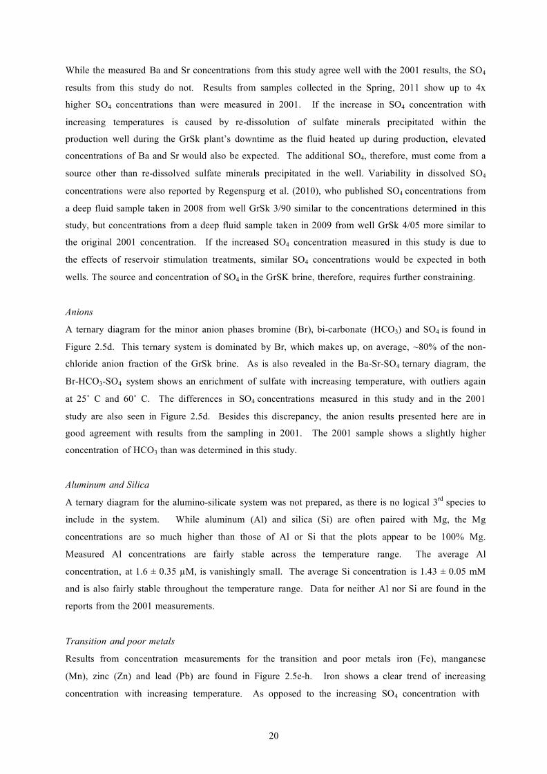
20

While the measured Ba and Sr concentrations from this study agree well with the 2001 results, the SO4

results from this study do not. Results from samples collected in the Spring, 2011 show up to 4x

higher SO4 concentrations than were measured in 2001. If the increase in SO4 concentration with

increasing temperatures is caused by re-dissolution of sulfate minerals precipitated within the

production well during the GrSk plant’s downtime as the fluid heated up during production, elevated

concentrations of Ba and Sr would also be expected. The additional SO4, therefore, must come from a

source other than re-dissolved sulfate minerals precipitated in the well. Variability in dissolved SO4

concentrations were also reported by Regenspurg et al. (2010), who published SO4 concentrations from

a deep fluid sample taken in 2008 from well GrSk 3/90 similar to the concentrations determined in this

study, but concentrations from a deep fluid sample taken in 2009 from well GrSk 4/05 more similar to

the original 2001 concentration. If the increased SO4 concentration measured in this study is due to

the effects of reservoir stimulation treatments, similar SO4 concentrations would be expected in both

wells. The source and concentration of SO4 in the GrSK brine, therefore, requires further constraining. Anions

A ternary diagram for the minor anion phases bromine (Br), bi-carbonate (HCO3) and SO4 is found in

Figure 2.5d. This ternary system is dominated by Br, which makes up, on average, ~80% of the non-

chloride anion fraction of the GrSk brine. As is also revealed in the Ba-Sr-SO4 ternary diagram, the

Br-HCO3-SO4 system shows an enrichment of sulfate with increasing temperature, with outliers again

at 25˚ C and 60˚ C. The differences in SO4 concentrations measured in this study and in the 2001

study are also seen in Figure 2.5d. Besides this discrepancy, the anion results presented here are in

good agreement with results from the sampling in 2001. The 2001 sample shows a slightly higher

concentration of HCO3 than was determined in this study. Aluminum and Silica

A ternary diagram for the alumino-silicate system was not prepared, as there is no logical 3rd species to

include in the system. While aluminum (Al) and silica (Si) are often paired with Mg, the Mg

concentrations are so much higher than those of Al or Si that the plots appear to be 100% Mg.

Measured Al concentrations are fairly stable across the temperature range. The average Al

concentration, at 1.6 ± 0.35 µM, is vanishingly small. The average Si concentration is 1.43 ± 0.05 mM

and is also fairly stable throughout the temperature range. Data for neither Al nor Si are found in the

reports from the 2001 measurements. Transition and poor metals

Results from concentration measurements for the transition and poor metals iron (Fe), manganese

(Mn), zinc (Zn) and lead (Pb) are found in Figure 2.5e-h. Iron shows a clear trend of increasing

concentration with increasing temperature. As opposed to the increasing SO4 concentration with

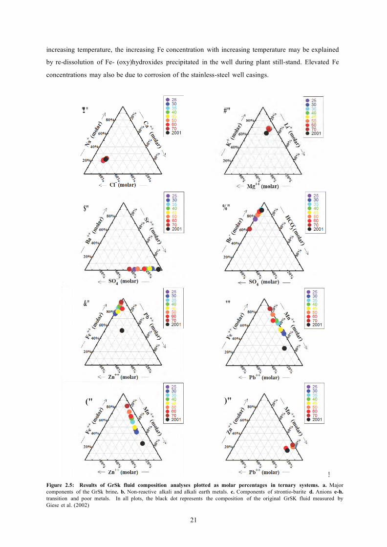
21

increasing temperature, the increasing Fe concentration with increasing temperature may be explained

by re-dissolution of Fe- (oxy)hydroxides precipitated in the well during plant still-stand. Elevated Fe

concentrations may also be due to corrosion of the stainless-steel well casings.

!" " #"

$" %"

&" '"

(" )"

!

Figure 2.5: Results of GrSk fluid composition analyses plotted as molar percentages in ternary systems. a. Major components of the GrSk brine. b. Non-reactive alkali and alkali earth metals. c. Components of strontio-barite d. Anions e-h. transition and poor metals. In all plots, the black dot represents the composition of the original GrSK fluid measured by Giese et al. (2002)

22

That fact that all samples contain significantly higher Fe concentrations than reported in the original

2001 results suggests the latter case to be more likely. Similar to Fe, Pb also shows a trend of

increasing concentration with increasing temperature. Because no Pb is contained in the well casing,

this observation can either be explained by dissolution of Pb-bearing phases in the well as the

produced fluid heats up or by chemical heterogeneities in the reservoir. The Pb-bearing phases

laurionite and native Pb have already been identified as scales in the GrSk system (Regenspurg et al.,

2010; Holl et al., 2003). The Pb concentrations measured in this study, especially at higher

temperatures, are also noticeably higher than those measured in the 2001 study. Zinc and Mn

concentrations are in good agreement with results from the 2001 study and remain fairly constant

throughout the temperature range. The measured Zn concentration is 0.61 mM at all temperatures.

The average measured Mn concentration is 2.30 ± 0.1 mM. The total CBE for all measured cation and anion species is -5.7%, which, considering the challenges in

analyzing high ionic strength fluids (e.g. Kühn et al., 2007) represents an internally consistent analysis.

Not only are the measurements internally consistent, they are also generally in agreement with the

initial analysis of the GrSk brine performed by Giese et al. (2002). The similarities between the data

presented in this study and the data from Giese et al. (2002) suggests that the effects of reservoir

treatments on the pristine formation fluid, as described by Regenspurg et al. (2010) have been largely

eliminated. Notable exceptions to this conclusion are the elevated concentrations of SO4, Fe and Pb

found in this study compared to the pristine data. It is certainly not coincidence that these three species have been previously identified (e.g. Regenspurg

et al., 2010; Holl et al., 2003; Seibt and Wolfgramm, 2003; Giese et al., 2002) as major components in

predicted scale-forming minerals in the GrSk system. Detailed investigations of Fe and Pb behavior

are beyond the scope of this work and are not further discussed. Accurate knowledge of the brine’s

SO4 concentration, however, is essential for reliable prediction of alkali-earth metal sulfate scaling

risks. The challenges involved in establishing a species’ average composition in sedimentary basin

brines, such as recognizing local compositional heterogeneities, preventing chemical reactions during

fluid transport to the laboratory and analytical uncertainties, are discussed, for example, by Hanor

(1993). Eugster and Jones (1979) report that dissolved SO4 may accumulate in a sedimentary basin

until Na2SO4 saturation is reached—a concentration much higher than results reported for the GrSk

fluid. Rotliegend brine chemistry, specifically, is described as a mixture between connate waters

present during the Rotliegend’s deposition and SO4-saturated waters from the overlaying Zechstein

(Platt, 1993). Analyses of sulfur isotopes in Rotliegend cements confirm the presence of Zechstein-

originated SO4 in Rotliegend pore waters (Gluyas, et al., 1993). The mixing of water infiltrated

through the Zechstein with connate waters from the Rotliegend suggests that considerable

23

heterogeneities (with respect to SO4) may exist in the Rotliegend brine. The variations in SO4

measurements between the original 2001 sampling (Giese et al., 2002), the report of Regenspurg et al.

(2010) and this study, therefore, are not inconsistent with natural processes and are not necessarily the

result of stimulation treatments in the reservoir or analytical error. Although the range of SO4

concentrations reported in the GrSk brine (i.e. ~1-4 mM) is rather small, the true sulfate concentration

remains elusive. An attempt to further constrain the SO4 concentration in the GrSk brine with use of

mineral stability diagrams (e.g. Bazin et al., 1997) is found in Chapter 3 of this work.

2.3.2 Mass fraction of solid phase in produced GrSk brine The results of the mass fraction experiments are plotted across the temperature range 20˚ - 70˚ C in

Figure 2.6. The mass fraction of solid phases in the GrSk brine appears to have a slightly increasing

trend with increasing temperature up to 70˚ C, where the value of the mass fraction spikes

dramatically. The measured solid mass fractions range from 0.0001 at 30˚ C and 35˚ C to 0.0011 at

70˚C. The average mass fraction of solid phases is 0.0004 ± 0.0003. The large standard deviation of

the measurement is due to the inflated result at 70˚ C. If this calculation is assumed to be an outlier,

the apparent trend of increasing solid mass fraction with increasing temperature becomes much less

pronounced, and the new average mass fraction is 0.0003 ± 0.0001. A metric ton (1000 kg) of the

GrSk brine, therefore, contained a base-load of ~300-400 g of solid phases during production testing in

the Spring of 2011.

Figure 2.6: Mass fraction of solid material in the GrSk brine versus temperature during production.

24

2.3.3 Chemical analyses of filter residue from the GrSk in-line filtration system

Three samples from the 2 µm pore size filters and 6 samples from the 10 µm pore size filters were

analyzed with XRF for chemical composition. Selected data from the XRF measurements are

displayed in Table 2.1. Graphical representations of the relationships between various chemical

components of the filter residue in mols/kg of precipitant are found in Figure 2.7.

Table 2.1: Measured elemental concentrations of solid matter found in GrSk in-line filter samples, i.e. moles of element per kg of filter residue (sample preparation performed in part by Sophia Wagner, GFZ).

Sample Si (M) Al (M) Fe (M) Ca (M) Na (M) Cl (M) 2 µm #1 0.08 0.20 1.49 3.61 3.60 13.82 2 µm #2 0.46 0.27 1.90 3.03 2.54 8.87 2 µm #3 0.09 0.26 1.04 3.59 3.57 15.91

10 µm #1

1.29

0.45

2.71

1.72

1.11

2.82 10 µm #2 0.38 0.45 2.35 3.23 2.16 10.78 10 µm #3 0.76 0.45 2.48 2.30 1.78 8.49 10 µm #4 1.24 0.83 4.07 1.37 1.12 5.20 10 µm #5 2.16 0.81 3.83 1.26 1.19 3.35

10 µm #6 2.81 0.95 5.05 0.20 0.00 0.10

Sample Ba (M) Sr (M) S (M) Cu (M) Pb (M)

2 µm #1 0.08 0.05 0.08 0.10 0.03 2 µm #2 0.26 0.07 0.15 0.32 0.16 2 µm #3 0.04 0.04 0.05 0.02 0.01

10 µm #1

0.43

0.09

0.90

0.34

10 µm #2 0.07 0.04 0.06 0.06 0.04 10 µm #3 0.17 0.04 0.14 0.45 0.19 10 µm #4 0.12 0.02 0.07 0.10 0.07 10 µm #5 0.11 0.02 0.07 0.09 0.06

10 µm #6 0.14 0.03 0.07 0.16 0.06

In the 10 µm filters, iron oxide (Fe2O3) is the most abundant metal oxide (~20-40%). Calcium oxide

(CaO; ~7-20%), silicon dioxide (SiO2; ~2-17%) and sodium oxide (Na2O; ~3-7%) are also prominent

amongst the oxides in the 10 µm filters. The last sample from the 10 µm filters (10 µm #6), however,

is strongly depleted in calcium and sodium oxides (CaO ~1%; Na2O < 0.01%). More CaO (~17-20%)

and Na2O (~8-11%) are found in the 2 µm filter than in the 10 µm filter. The difference in CaO and

Na2O fractions between the 10 µm and 2 µm filters is also reflected in the difference in Cl fractions

between the 2 filter sizes. Chlorine fractions range from ~12-40% in the 10 µm filter and ~50-57% in

the 2 µm filter. The additional CaO and Na2O in the 2 µm filters is accompanied by a decrease in both

Fe2O3 and SiO2 mass percent from the 10 µm filters to the 2 µm filters. The mass percentage of Fe2O3

in the 2 µm filter ranges from ~8-15%, about half the concentration as found in the 10 µm filter. The

25

SiO2 mass percentage in the 2 µm filter ranges from ~0.5-3%. Aluminum oxide (Al2O3) mass

percentages range from ~2-5% in the 10 µm and ~1-1.5% in the 2 µm filter. The water loss on

ignition (LOI) ranges from ~12-25% in the 10 µm filters and ~10-13% in the 2 µm filters. The

fractions of Mg, Mn, Ti, K and P oxides are less than 1% in all filters; these oxides have been

excluded from the data in Table 2.1. Amongst trace elements, Ga, Nb, Ni, Rb, V, Y, Zn, Zr, As , Mo and Cr all have mass fractions of

<0.001% of the total mass and have, therefore, also been excluded from the data in Table 2.1.

Although Ba is usually considered a trace element, its mass fraction in the precipitant can be as high

~6%. Generally, more barium is found in the larger filter size than the smaller. No significant

difference in Sr mass fractions is observed between the two filter sizes. The Sr mass fractions range

from 0.34-0.64% in the 2 µm filter and from 0.20 -0.77% in the 10 µm filter. Both Pb and Cu are

more concentrated in the larger-pore filter than the smaller pore filter. In the 2 µm filter, Pb and Cu

mass fractions range from 0.12-3.25% and 0.15-2.00%, respectively. The ranges for Pb and Cu mass

fractions in the 10 µm filter are 0.75-7.15 and 0.60-5.73, respectively. Mass fractions reported above are converted into mols/kg of precipitant, allowing individual

precipitated species in the filter to be compared with one another on a molar basis. These comparisons

are found in Figure 2.7a-f. In Figure 2.7a, Ca and Na are plotted individually and as a sum against Cl.

If the Cl predominately precipitates as NaCl, the slope of Na vs. Cl plot should be 1. In a similar

manner, if the Cl predominantly precipitates as CaCl2, the slope of the Ca vs. Cl plot should be 0.5.

The data shows a Na:Cl molar ratio of ~0.2 and a Ca:Cl molar ratio of ~0.33. When Na and Ca are

summed, the Na+Ca:Cl: ratio is ~0.5. These results suggest that Cl precipitates mostly as CaCl2, but

the total Cl precipitation cannot be attributed to Na and Ca alone. Figure 2.7b shows the relationships between Ba, Sr, and S. That sulfur is expressed as S and not SO4

is irrelevant, because, whether written as S or SO4 only a single mole of S is contained per mole of

[Ba+Sr] in strontio-barite, or per mole of Ba or Sr in the end-member phases. A slope of 1 is,

therefore, expected in the plot of either Ba or Sr vs. S. The best fit to this hypothesis is found in the

plot of Ba+Sr vs. S, which has a slope of ~0.65. This result suggests that S precipitation is not limited

to the stontio-barite system. All of the Ca, however, is required to account for Cl precipitation,

making it unlikely that the missing sulfate phase bears much Ca. There is no discernable relationship between precipitated Si and Al amounts, as seen in Figure 2.7c.

This observation, coupled with the generally greater molar amount of Si in the precipitant compared to

Al, suggests that no clays or zeolites are precipitating from the produced fluid, and Si precipitation is

predominantly SiO2.

26

!"

#"

$"

!

Figure 2.7a-c: Plots of molar relationships between precipitated species measured by XRF analysis. A. Na-Ca-Cl system B. Ba-Sr-S system C. Si-Al system

27

!"

#"

$"

!

Figure 2.7d-f: Plots of molar relationships between precpitated species measured by XRF analysis. d. S-Cl system e. Pb-Cu system f. Fe-Pb-Cu system.

28

Similar to the Si vs. Al plot, no clear relationship exists between Cl and S precipitation, as shown in

Figure 2.7d. These anions species clearly behave independently from one another in the GrSk brine.

Figure 2.7e shows a strong linear relationship (r2=0.99) between Pb and Cu concentrations in the filter

residue. Copper concentrations as a molar quantity in the filter residue are nearly 3 times higher than

Pb concentrations. Whether or not Pb and Cu are precipitated in a single phase must be determined by

other methods (see below), but from this data it appears that Pb- and Cu- bearing mineral precipitation

are governed by the same conditions in the fluid. When these species are compared to Fe, as shown in

Figure 2.7f, no clear relationship between the species’ is seen. This observation suggests that, while

Pb and Cu precipitation is strongly related, Fe behaves independently from these other metals in the

GrSk brine.

2.3.4 Mineralogical analyses of filter residue from the GrSk in-line filtration system

All 9 filter samples described above were analyzed with XRD and SEM. Graphs of the XRD results

are found in Figure 2.8. Selected photo-micrographs, along with associated EDX spectra from the

SEM analyses are displayed in Figure 2.9-11. The XRD analyses reveal halite (NaCl) and strontio-

barite ([0.75 Ba:0.25 Sr]SO4) ) in all nine filter samples. Halite is believed to precipitate as the filter

dries, not as a consequence of oversaturation in the brine. The ubiquitous presence of strontio-barite

in the filters confirms the hypothesis presented in the introduction to this work, namely, that alkali-

earth metal sulfates are a primary scaling risk in the GrSk plant. Magnetite (Fe3O4) is found in all 6 of

the 10 µm filters and one of the 2 µm filters. The reduced Fe phase requires that the fluid’s redox

potential (Eh) is less than ~350 mV (Takeno, 2005). If precipitation occurred during the time between

the filters were changed at the plant and the time of the sample preparation and analysis, an oxidized

iron phase (i.e. hematite; Fe2O3) would be expected. As discussed in Chapter 3 of this work, the

simultaneous presence of magnetite and sulfate can be used to constrain the otherwise heretofore

ambiguous redox potential of the GrSk brine. Quartz (SiO2) is absent from all of the 2 µm filters, yet

unambiguously present in 1 of the 10 µm filters. Quartz may be present in at least 3 additional 10 µm

filters, but the quartz peak’s proximity to the strontio-barite peaks confounds the results. The overlap

between these two minerals’ XRD spectra peaks is further augmented by the fact that, with the

exception of halite, none of the XRD peaks are especially well defined. The somewhat diffuse nature

of the XRD spectra reveals that the majority of the filter residue is weakly to non-crystalline.

Nonetheless, strontio-barite as a crystalline phase has been definitively identified.

29

[

- "' ......

- t:l

l

I

r

::c I'> c=: (;

I f · -· L.€

l ' ' I

-·' • I -·

· - r-- 0 0 N

§ § 3

,_ t ' ;>-

fl

*.j>. "" '*

(/<1 t:l

n

, ·••u'''t'U lilt tIt t t U Ill f t'

' ' I I -·I I I I I I-I

-.J

0 l 0 N

t a 3 8

[B *v. N"" VI H '<f?.

0 to s·

I I

N

l ""

"' "'!. ..... .... ........ c'r"

::: 0

I II t I • t I I & Ij t I f.

.l t

0 0

30

r t I t

...

I - 8 3 '"*' '"*'

I

Figure 2.8: X-ray diffraction pattems for solid material taken from three 2 pm filters and six lOpm r.Jters (samp., pn•parationp1-ovided in part by Sophia Wagner, GFZ).

31

!"

#"

!

Figure 2.9a-b: Photomicrographs of (1) weakly crystalline aggregate of solids and (2) iron oxide, with accompanying EDX spectrographs, collected from the in-line GrSk filtration system during production testing in 2011. The photos are taken at 1.01 kx (upper) and 2.32 kx (lower). The weakly crystalline masses comprise the majority of the GrSk filter residue. The iron oxide, identified by the EDX spectrum, is assumed to be magnetite, based on the XRD results (unpublished photos provided by Sophia Wagner, GFZ).

32

# !

"

!$

"$

#$

!

Figure 2.10: Photomicrograph of laurionite with copper and barite, collected from the in-line GrSk filtration system during production testing in 2011. 1. Clean laurionite (PbCl[OH]) 2. Laurionite with adsorped copper-bearing phase, perhaps malachite (based on presence of C) 3. Barite. EDX plots shown beneath the picture reveal the chemical make-up of the associated points (1-3). The photo is magnified 1.79 kx (unpublished photos provided by Sophia Wagner, GFZ.)

33

I,.-

' .. ' ' '" ..,

".., ...

Ska l ietung, Count ;:

t! I 'l , o · ' 1 t 1\ " I ...,,,... ,

""

25000

s 20000 Ba

t5000

Sr 10000

5000

0 == ======== 0

m - 6 - C 2 4 8 10

ktV

'> 1> 1 "''''' I > ,..- tl I'I , 0 · ' I t 1\ " I I. .. ,.,. >

Ska l ierung. Counts: t5406

20000

s 0 Mo

" 'I t I I I I I It" I n 1 U II l'" '""I' • .I.J" >, ,• IIt

1$000 Fe

10000 Ba

m -26- Ft

keV

Cu

8 10

Figure 2.11: Photomicrographs of well-crystallized barite, with accompanying EDX spectrographs, collected from the in-line GrSk mtration system during production testing in 2011. The upper photo is magnified 1.32 kx. The lower photo is magnified 2.74 kx (unpublished photos provided by Sophia Wagner, GFZ).

34

The SEM analyses confirm the results of the both the XRF and XRD analyses. Optical analyses reveal

most of the filter residue to be poorly crystalline aggregates of many different chemical species.

Selected photographs and a representative EDX spectrum of these aggregates is found in Figure 2.7a.

Many of the chemical species found in the aggregates, most notably Pb and Cu, are not identified in a

mineral phase by the XRD, but are detected in significant quantities by the XRF. Figure 2.7b, shows

an iron oxide, assumed to be magnetite based on the XRD results. The lead bearing phase laurionite

(PbCl[OH]) appears in a crystalline form, in some cases covered with a layer of an adsorbed copper-

bearing bearing mineral (Figure 2.7c). The presence of carbon in the EDX spectrum for Figure 2.7b

suggests that this mineral may be malachite. Once again confirming the results from the XRD

analysis, strontio-barite is the most abundant and best crystallized phase in the GrSk filter residue. A

selection of photographs of strontio-barite, along with associated EDX spectra is found in Figure 2.7d.

Quartz was not observed with the SEM, but SiO2 was present as an amorphous phase in many of the

chemical aggregates depicted in Figure 2.7a.

2.4 Conclusion

Fieldwork performed at the GrSk site during production testing in the Spring of 2011 is presented in

this chapter. The chemical composition of fluid produced in the GrSk 4/05 well from a depth of

~4300 m in the Permian Rotliegend sandstone is analyzed as a function of temperature. The mass

fraction of advectively transported solids in the produced fluid is calculated, and the chemical and

mineralogical composition of solid material removed from the plant’s in-line filtration system is

determined. Generally, the composition of the fluid from these production tests are in good agreement with the

original fluid analysis performed by Giese et al. (2002) upon re-opening of the GrSk 3/90 well in

2001. The agreement between the data presented here and the 2001 data suggest that the effects of

reservoir stimulation procedures on the in-situ fluid’s chemistry, as described by Regenspurg et al.

(2010) are no longer influencing the brine’s chemistry. The concentrations of Fe, Pb and SO4,

however, are not in good agreement with the 2001 data. These species have been identified as scale-

forming mineral components (e.g. Regenspurg et al., 2010; Holl et al., 2003) in the GrSk system. The

differences in these species’ concentrations determined in this study and the 2001 study reflect the

dynamic state of the GrSk fluid during production and are indicative of active precipitation/dissolution

processes within the power plant infrastructure. Results for the solid mass fraction study presented

herein suggest that up to 400 g of solid are present in 1 metric ton of brine. This result, however, may

35

be more reflective of debris transport up the well from the reservoir, rather than precipitation from the

brine. Solid phase analyses performed during this study are in excellent agreement with the previous results

of Holl et al. (2003), who reported incidents of laurionite, malachite, native Pb and barite scaling on

the plant’s pump, well casing and scales after production testing in the GrSk 3/90 well in 2001. X-ray

diffraction measurements and SEM analyses performed during this study confirm the presence of well-

crystalized (stontio-)barite in the GrSk brine. This study also detected laurionite with the SEM, but

not with the XRD. Similar to barite, the observed laurionite is well crystallized and, in some cases,

covered with a Cu-bearing phase. Whether or not the Cu-phase is malachite or native copper is

unclear. X-ray diffraction also revealed the presence of magnetite and quartz in the filter residue, but,

whereas magnetite was observed as a crystalline phase with SEM, quartz was not. Most of the filter

residue was poorly to un-crystalized. Results from the fieldwork in this study conclusively show that, as hypothesized, strontio-barite is a

primary scaling hazard in the GrSk system.

36

3. Ion activities and mineral solubilities in the Na-Ca-Ba-Sr-Cl-SO4-H2O system at

conditions found in the Groß Schönebeck geothermal loop

37

∆!!

3.1 Introduction After the re-opening of the GrSk 3/90 well in 2001, and the subsequent chemical analysis of the

Rotliegend formation fluid taken at depth, a preliminary model of the GrSk fluid was constructed with

the SOLEMINEQ.88 program (Kharaka et al., 1988) by Giese, et al. (2002) with a particular focus on

(1) chemical geothermometry and (2) changes in the saturation indices (SI) of select minerals with

temperature. The SI variable is defined below. Based on quartz geothermometry, Giese et al. (2002)

calculated reservoir temperatures to be between ~170˚ and 190˚ C. Dolomite and quartz were

identified as oversaturated phases at 150˚ C, and barite, quartz and amorphous SiO2 were identified as

oversaturated at 25˚ C. (Giese et al., 2002). Based on models created with PHREEQc (Parkhurst et al.,

1995), Regenspurg et al. (2010) discuss the scaling potential of several sulfate and carbonate minerals

within the GrSk system, suggesting that precipitation within these mineral groups is controlled by the

relevant anions’ concentrations. Regenspurg et al. (2010) also discuss the potential precipitation of

several transition (i.e. Fe, Mn) and poor (i.e Zn, Pb) metals as being controlled by changes in the

fluid’s redox condition. While Regenspurg et al. (2010) cite calculations with PHREEQc as the source

of their scaling predictions, they do not describe the parameters, database or methods used in the

model calculations. Thus, at present, no rigorous geochemical modeling of scaling risks in the GrSk

system has been performed. The purpose of this chapter, therefore, is to construct a detailed

thermodynamic equilibrium model of the Na-Ca-Ba-Sr-Cl-SO4-H2O system at the (T, p, x) conditions

found in the GrSk thermal loop.

Mineral solubilities in aqueous solutions are a function of the mineral’s equilibrium constant (Ksp) and

the ion activity product (IAP) of the free ions involved in the mineral’s formation. Known as the

saturation index (SI), the quotient of these two variables describes a mineral’s relationship to the

equilibrium state:

(eq. 3.1) 𝑆𝐼 = !"# !!"

where SI is the saturation index, IAP is the ion activity product and Ksp is the mineral’s equilibrium

constant (Drever, 1997). If the IAP > Ksp, the mineral is oversaturated and may precipitate from

solution (Drever, 1997). If the IAP < Ksp, the mineral is undersaturated and may dissolve if placed in

solution (Drever, 1997). If the IAP = Ksp the precipitation/dissolution reaction is in equilibrium, and

there will be no further chemical action in the system (Drever, 1997). A mineral’s Ksp is a function of

the standard state Gibbs’ free energy of the reaction:

! (eq. 3.2) 𝑙𝑜����!" = −

!.!"!!"

38

!!! !

where ΔGr0 is the standard state Gibbs’ energy of reaction, R is the gas constant and T is the

thermodynamic temperature. The standard state is defined throughout this text as 298.15 K and 0.1

MPa. Equilibrium constants, along with all other partial molal thermodynamic properties, for a large

selection of chemical species and reactions can be calculated for temperatures up to 1000˚ C and

pressures up to 500 MPa using the SupCrt program (Johnson et al., 1992). Equilibrium constants

calculated by SupCrt are the basis for equilibrium models computed in several geochemical modeling

programs, such as PHREEQc and the Geochemists’ Workbench (Bethke, 2008; Parkhurst et al., 1995). Determining the activities of dissolved ions, and thus the IAP of system, is not as straightforward as

determining a reaction’s Ksp. In an ideal, infinitely dilute solution, an ion’s activity is simply equal to

its concentration (Drever, 1997). In reality, however, dissolved components in solution affect the

solution’s ionic strength, leading to the formation of aqueous complexes (Drever, 1997). Aqueous

complexes alter the effective concentration of a dissolved component without removing that

component from the solution in the form of mineral precipitants. The effective concentration of an ion

in solution, after consideration of aqueous complex formation, is known as the ion’s activity and is

defined by:

(eq. 3) αi = γimi

where αi is the activity of species i, m is the molal concentration of species i and γi is species i’s

activity coefficient. In solutions with ionic strength < 0.1 m, activity coefficients are determined by

some form of the Debye-Hückel equation:

(eq. 4) 𝑙����𝛾 = −��𝑧 ! !

!!!!! !

where γD-H is the activity coefficient according to the Debye-Hückel theory, z is the charge of species i, I

is the solution’s ionic strength, A and B are empirically fitted parameters for a defined temperature

and ao is a parameter related to the minimum distance between ions in the solution.

The Debye-Hückel theory (Debye and Hückel, 1923) adjusts ion activities based on electrostatic

interactions between individual ions and the surrounding solution (i.e. long-range Coulomb forces).

As a solution’s ionic strength increases, however, ions come within increasingly closer proximity to

each other. Therefore, activity coefficient determinations in high ionic strength (> 0.1 m) solutions

must consider not only interactions between ions and the surrounding solution, but also between

different individual ions in solution (e.g Harvey and Weare, 1980). The theoretical considerations of

specific ion interactions in aqueous media and the virial mathematical expansions that define these

interactions were first described by the working group of Kenneth Pitzer in the 1970s (Pitzer and Kim,

39

1974; Pitzer and Mayorga, 1974; Pitzer and Mayorga, 1973; Pitzer, 1972). The fundamental Pitzer

equation is an expansion of the Debye-Hückel equation that, in addition to consideration of the long-

range forces affected by the solution’s ionic strength, also considers interactions between specific pairs

(2nd virial expansion) and groups (subsequent virial expansions) of ions, as follows

(eq. 5) 𝑙������! =

𝑙������!!! +

!,! ��!" ��!

��! +

!,!,! ��!,!,! …

where logγD-H is the activity coefficient calculated from the Debye-Hückel equation and λ and µ are

empirically derived parameters describing the interaction between pairs and triads of specific ions

([i,j]; [i,j,k]) in solution (Bethke, 2008). Several authors have demonstrated the Pitzer formulations’

accuracy in geochemical models (e.g. Millero, 2009: Greenberg and Moller, 1989; Harvey et, al.,

1984; Harvey and Weare, 1980). Moller and Weare (1999) have extensively discussed the application

of Pitzer formulations to geothermal systems.

Pitzer parameters for aqueous species have been compiled into a number of thermodynamic databases,

several of which are included in the Geochemists’ Workbench (GWB) modeling program (Bethke,

2008). The GWB can emulate the Pitzer database included with the PHREEQc modeling program (i.e.

thermo_phrqpitz), or can employ one of its own databases (i.e. thermo_hmw, thermo_hdata,

thermo_pitzer; Bethke, 2008). The thermo_phrqpitz and thermo_hmw databases are the most up-to-

date of the selections, but are severely limited when applied to the (T, p, x) conditions found in

formations fluids, in general, and the GrSk brine, specifically (Bethke, 2008). Neither of these

databases, for example, contains the necessary thermodynamic data for modeling barite, rendering

these databases essentially useless for this study. The other Pitzer databases incorporated in the GWB

(thermo_hdata, thermo_pitzter) are considered outdated. These databases are included in the current

versions of the GWB for compatibility with older editions of the software, but their use is discouraged

(Bethke, 2008). The thermo_pitzer database, however, is the only Pitzer database included with the

GWB that contains thermodynamic data for barite, and is, therefore, the program’s only database

suitable for modeling the GrSk system. Another Pitzer database compatible not with the GWB, but

with the PHREEQc program, is the Quintessa database. Although this database contains updated

thermodynamic parameters for all the aqueous and mineral species required for modeling the behavior

of the GrSK brine, the data has not been peer-reviewed. None of the existing Pitzer thermodynamic databases are perfectly suited to modeling the behavior of

the GrSk brine as it traverses the systems geothermal loop. Choosing the best database to use in the

model is somewhat of an arbitrary decision. Only the thermo_pitzer database in the GWB and the

QNT database for PHREEQc contain all the parameters necessary for geochemical modeling of the

GrSK system. For the sake of continuity with more advanced modeling features (such as activity-

activity diagrams and reaction path modeling) found in the GWB but not found in PHREEQc, this

40

study employs the thermo_pitzer_ database to model aqueous species activities in the Na-Ca-Ba-Sr-

41

Cl-SO4-H2O system at the GrSk (T, p, x) conditions. The model presented here is the first model of

the GrSk brine designed to show specifically what minerals within the alkali-earth metal sulfate

system may precipitate at different locations along the GrSk geothermal loop.

3.2 Methods

3.2.1 Calculating effects temperature and pressure on the logKsp of anhydrite and barite

The effects of temperature and pressure on the Ksp of anhydrite and barite are calculated with SupCrt.

The existing thermodynamic database (dprons92) is used as the basis, and calculations are made in the

single-phase region (as opposed to the along the liquid-vapor saturation curve). Temperature and

pressure are used as independent state variables, and the univariant curve option is turned off.

Calculations are performed under isothermal conditions at pressures from 0.1-4.5 MPa. A discrete

calculation with the given pressure range is made at 10˚ C intervals from 20˚ - 200˚ C. In other words,

18 different calculations are performed and sewn together to complete the model. Results are plotted

in 3-D, logKsp–temperature–pressure space.

3.2.2 Aqueous speciation of the GrSk brine from 25˚ C to 150˚ C Basis system parameters (i.e. pH, density, ionic strength) and ion activities as a function of

temperature in the Na-Ca-Ba-Sr-Cl-SO4-H2O system at GrSk concentrations are calculated with the

GWB thermo_pitzer database in the REACT program, contained in the GWB. Average species’

concentrations from the fieldwork presented in Chapter 2 of this work (Table 3.1, below) are used as

basis inputs in the calculations. Although Giese et al. (2002) reported pH values of 5.7 and 5.9 in

GrSk 3/90 samples taken at depth, the use of standard glass pH electrodes in highly saline brines is

considered unreliable (Millero et al., 2009). In the absence of any other data, however, the average

value (pH = 5.8) is used as the input pH, and the model calculates the change in pH with temperature.

Regenspurg et al. (2010) reported redox potentials ranging from -129 – -174 mV for the GrSk brine,

but did not explain how these measurements were made. Based on the Eh-pH diagrams for sulfur

species found in the Atlas of Eh-pH diagrams (Takeno, 2005), these Eh values these values appear

slightly low; to ensure that the redox potential supports the stability of SO42-, an Eh of 0 is used as the

input. This value also supports the stability of magnetite over hematite, as reported in Chapter 2 of

this study.

42

The initial and final temperatures are set to 25˚ C and 150˚ C, respectively. The GWB does not allow

for adjusting the pressure during the calculations; all speciations are performed at the liquid vapor

saturation curve. The loss of liquid water to the vapor phase at T > 100˚ C is offset by selecting 1 kg of

solvent, as opposed to 1 kg of free solvent. This selection tells the program to consider 1 kg of liquid

water as the solvent at all temperatures, rather than having 1 kg of total water partitioned between the

liquid and vapor phases. The concentration of Cl is adjusted to compensate for charge imbalances. To

improve the accuracy of the model, the results from the SupCrt calculations (Section 3.2.1) are

incorporated into the program by choosing “alter logK” in the “config” drop-down menu. To calculate

the ion activities of the oversaturated fluid, the program is run with the “precipitation” option turned

off.

Table 3.1: Geochemists’ Workbench speciation model input concentrations (molarity)

Chemical Species (Molarity)

Na+ Ca2+ Ba2+ Sr2+ Cl- SO42- H2O (kg)

1.45 1.1 0.00027 0.0114 4.25 0.004 1

3.2.3 Stable phase assemblages

Stable phase assemblages at each point along the GrSK geothermal loop are calculated at discrete

temperatures and pressures with the ACT2 program included with the GWB. Activity-activity

diagrams are created to represent (1) reservoir conditions at the production well (150˚ C; 45 MPa), (2)

the hot side of the heat exchanger (150˚ C; 0.1 MPa), (3) the cold side of the heat exchanger (75˚ C;

0.1 MPa) and (4) reservoir conditions at the injection well (75˚ C; 45 MPa) Input activities for the

relevant temperatures are chosen from the calculations performed in 3.2.2. The logKsp for the relevant

temperatures and pressures are chosen from the calculations performed in 3.2.1. Stable sulfate

assemblages are plotted as functions of calcium/barium activities.

3.2.4 Polythermal reaction path model Polythermal reaction paths for anhydrite and barite as the GrSk fluid cools across the heat exchanger

are modeled with GWB’s REACT program by running the script described in 3.2.2 above with the

“precipitation” option activated in the Config drop-down menu. For easy comparison with the field

study presented in Chapter 2 of this work, mineral precipitation is calculated on a gram per m3 of brine

basis. The molar quantities presented in Table 3.1 are, therefore, considered in 1000 kg of solvent (not

free solvent) for the calculation of the reaction path. To account for the GrSk brine’s ambiguous

43

sulfate concentration (Chapter 2, discussion), reaction paths are computed for sulfate concentrations

from 0.5 mM to 5 mM

3.3 Results

3.3.1 Temperature and pressure effects on the logKsp of anhydrite, barite and celestite

Plots of temperature vs. pressure vs. logKsp for anhydrite, barite and celestite are found in Figure 3.1.

As shown in Equation 2 above, the logKsp is a function of the negative Gibbs’ energy of a reaction.

Approach to equilibrium minimizes Gibbs’ energy, and the reaction is entered into SupCrt as the

formation of the solid phase (i.e Ca + SO4 ß CaSO4). Therefore, a decreasing slope in the

logKsp plot corresponds into an increase in the Gibbs’ energy, and thus the increased stability of the

reactants. Hence, decreasing slopes in the logKsp–temperature–pressure space correspond to an

increased mineral solubility. Anhydrite

The anhydrite logKsp ranges from ~3.5-7.5, with the minimum at 25˚ C and 45 MPa and the maximum

at 150˚ C and 0.1 MPa. Anhydrite solubility increases with increasing pressure and decreases with

increasing temperature. The anhydrite logKsp trends vs. both temperature and pressure are sub-linear.

The effects of temperature are more pronounced than the effects of pressure, i.e. the decreased

solubility caused by high temperatures in the reservoir nullifies the increased solubility caused by

reservoir pressures. Barite

Within the given temperature and pressure constraints (i.e. 20˚ - 200˚ C; 0.1 – 45 MPa), the logKsp of

barite ranges from ~9-10.25, with the minimum at 45 MPa and ~100˚ C and maxima at 20˚ C and 200˚

C at 0.1 MPa. While barite is several orders of magnitude less soluble than anhydrite, the effects of

temperature and pressure on barite solubility are not as strong their effects on anhydrite. Similar to

anhydrite, barite solubility increases with increasing pressure. The temperature effects on barite

solubility, however, are not linear. According to the SupCrt calculations shown here, barite solubility

increases from ~20-100˚ C before decreasing again from ~100-200˚ C. Celestite

Temperature and pressure affects the logKsp of celestite in a similar manner to their effect on the

logKsp of anhydrite. Celestite’s solubility decreases with increasing temperature and increases with

44

0

39

/

&%#

/

39

/

39

!"#$%&'() *+,-.

*#

$#

)# 2678 %#

+# 45,

%*#

&# !)# (#

*,*-)# $-),*# $,$-)# )-),$# ),)-)# &-),)#

(-),&#

((#

&%#

!"# $"#

%""# %&"# Û&

%'"#

1,&'() *1,-. 0

%"-!)#

%"#

%# +#

45,

%*#

!)#

+-*)# +-)#

+-!)# +#

2678

%",%"-!)# +-*),%"#

+-),+-*)# +-!),+-)# +,+-!)#

((#

!"# $"#

%""# %&"#

Û&

%'"#

+)2)3('() *-&-. 0 '#

*# 2678

%#

+# 45,

%*#

$#

!)# )#

*-),'# *,*-)#

$-),*# $,$-)#

)-),$# ),)-)#

((# &%#

!"#

$"# %""#

%&"# %'"#

Û& !

Figure 3.1: Effects of temperature and pressure on the logKsp of anhydrite, barite and celestite, calculated with SupCrt using, using the parameters described in section 3.2.1.

45

increasing pressure. The maximum solubility is found at 20˚ C and 45 MPa, while the solubility

minimum is at 150˚ C and 0.1MPa. Also similar to anhydrite, the temperature effect on celestite’s

logKsp exceeds the pressure effect. The overall solubility of celestite lies between that of anhydrite and

barite.

3.3.2 Aqueous speciation as a function of temperature in the Na-Ca-Ba-Sr- Cl-SO4-H2O system at GrSk concentrations

The molar concentrations of ions shown in Table 3.1 are speciated in 1 kg of water with the GWB’s

thermo_pitzer database in the REACT program. Diagrams displaying the effects of temperature on the

system’s basis parameters, ion activities and the saturation indices of selected minerals are shown in

Figure 3.2. The logKsp calculated in SupCrt were incorporated into the model, but the pressure did not

affect any noticeable differences in the results. Results presented here are for 0.1 MPa and represent

the effects of the temperature on the described parameters in the GrSk surface infrastructure. System basis parameters

Changes in the fluid’s pH, ionic strength and density as a function of temperature are shown

graphically in Figure 3.2a. The starting pH (i.e. @ 25˚ C) is 5.8. The pH decreases to 5.38 at 150˚ C

in a manner described by a 2nd order polynomial function. At 25˚ C, the fluid’s ionic strength is ~6.2,

and is constant until 75˚ C, where it decreases linearly to ~6.0 at 150˚ C. The fluid’s density decreases

linearly from 1.11 g/cm3 at 25˚ C to 1.03 g/cm3 at 150˚ C. Ion activities

Figure 3.2b shows the change in the activities of dissolved species in the GrSk fluid as a function of

temperature. The activity of water decreases sub-linearly from 0.85 to 0.80 across the temperature

range (25˚-150˚ C). The increase in the activities of both Na and Cl with increasing temperature can

be described as 2nd order polynomial functions. The activity of Na ranges from 1.06 at 25˚ C to 11.98

at 150˚ C. The activity of Cl ranges from 5.00 at 25˚ C to 11.71 at 150˚ C. The activities of Ca, Ba

and Sr all decrease with increasing temperature. The activities range from 0.34 – 0.07, 4.34e-5 –

1.69e-5 and ~0.003 – ~0.0007 for Ca, Ba and Sr, respectively, between 25˚ and 150˚ C. The activity

of SO4 increases non-linearly from 1.12e-4 at 25˚ C to 3.39e-4 at 150˚ C. Saturation Indices

Saturations indices (SI; IAP/Ksp) for anhydrite, barite, celestite and halite are plotted as a function of

temperature in Figure 3.2c. Saturation indices greater than 1 represent over-saturated minerals. Barite

is strongly super-saturated at all temperatures, with an SI ranging from 19.23 at 25˚ C to 13.74 at 150˚

46

Satu

ratio

n In

dex

Act

ivity

Va

lue

C. The decrease in barite’s SI is non-linear, with the minimum (11.88) appearing at 100˚ C.

Anhydrite remains undersaturated until ~60˚ C and becomes rapidly over-saturated in a linear fashion

with increasing temperature to an SI of 21.60 at 150˚ C. Both halite and celestite remain

undersaturated until high temperatures, i.e. > ~120˚ C for halite; > ~140˚ C for celestite.

10

pH

Ionic strength

Density

1

1.E+02 Cl-

1.E+01

1.E+00

1.E-01

1.E-02

1.E-03

1.E-04

Na+

H2O

Ca++

Sr++

SO4--

Ba++

1.E-05

1.E+02

1.E+01 Barite

1.E+00 Anhydrite

Halite

1.E-01

Celestite

1.E-02

0 25 50 75 100 125 150 175 7 Û&)

Figure 3.2: Calculated values for GrSk speciation model using thermo_pitzer database in the Geochemists’ Workbench. a. system basis parameters b. ion activities in super-saturated solution c. saturation index of selected minerals.

47

4

log_

(Ba2+

)

Anh

ydrit

e log_

(Ba2+

)

Anh

ydrit

e

3.3.3 Stable phase assemblages along the GrSk geothermal loop The Act2 program in the GWB can employ the logKsp determined in Section 3.3.1 and ion activities

calculated in Section 3.3.2 to model stable phase assemblages at various points along the GrSk

geothermal loop. Assemblages were calculated for 4 steps along the geothermal loop, as described in

3.2.3, above. As previously mentioned, the pressure variation made no discernable difference to the

diagrams; only results for the calculations at 0.1 MPa are shown here (Figure 3.3). The conditions

represented by the phase assemblage diagrams in Figure 3.3 correspond to the GrSk surface

installation before and after the heat exchanger.

D. 0 150Û & -1

b. 0 75Û & -1

0.1 03D -2 -3

-4

-5

-6

-7

Barite

0.1 03D -2

-3 Barite

-4

-5

-6

-7 -8

-9

-10

Celestite

-8

-9

-10

SO 2-

-10 -9 -8 -7 -6 -5 -4 -3 log_(Ca2+)

-2 -1 0 -10 -9 -8 -7 -6 -5 -4 -3 log_(Ca2+)

-2 -1 0

Figure 3.3: Stable sulfate phase assemblages as a function of calcium and barium activities in the GrSk brine at a. the hot side of the heat exchanger and b. the cold side of the heat exchanger. The stars represent the activities calculated with REACT for the GrSk fluid at the given temperatures. Inputs for background electrolyte activities, including sulfate, are taken from the results presented in 3.3.2, above.

On the hot side of the heat exchanger, the stable assemblage consists of anhydrite, barite and celestite.

Celestite is stable when the logα Ba is less than ~ -5.9 and the logα Ca is less than ~ -2.5. Above a

logα Ba of ~ -5.9, barite is stable. The barite/anhydrite equilibrium is represented by a line with a

slope of ~1 starting at the upper right corner of the box defining the celestite stability field. Ion

activities for Ca and Ba calculated in 3.3.2, above, place the GrSk fluid near the barite/anhydrite

equilibrium line, but slightly in the field of anhydrite. On the cold side of the heat exchanger, the

celestite stability field is replaced by aqueous SO42- as the stable sulfate phase below a logα Βa ~ -5.9.

Dissolved SO42- is stable up to a logα Ca of ~ -1.5. The dissolved SO4

2- stability field is slighter larger

in the direction of Ca than its celestite counterpart at 150˚ C. Similar to the 150˚ C diagram, the

barite/anhydrite boundary is represented by a line with a slope of ~1, beginning at the upper right

corner of the dissolved SO42- stability field. Calculated Ca and Ba ion activities at 75˚ C place the

GrSk fluid clearly in the barite stability field on the cold side of the heat exchanger.

48

gram

s per

m3

of b

rine

3.3.4 Reaction path model

The reaction of paths of anhydrite and barite as the GrSk brine cools from 150˚ - 75˚ C in the plant’s

heat exchanger are shown for 4 different sulfate concentrations in Figure 3.4. At all sulfate

concentrations, barite begins to form as the brine cools through ~135˚ C. For sulfate concentrations

between 1 and 5 mM, the amount of barite precipitation increases sub-linearly (not seen in the log-

scale axis in Figure 3.4) to a maximum at 75˚ C of ~60 grams of precipitant per m3 of brine. With an

initial sulfate concentration of 0.5 mM, barite precipitation reaches a maximum of ~40 grams of

precipitant per m3 of brine at 105˚ C. At this point, the mineral is no longer saturated with respect to

sulfate and precipitation stops.

1000

100

10

1

0.1 175

150

125

7 Û&)

100 75 50

Barite

0.005 M SO 2- 0.001 M SO 2- 4 4

Anhydrite 0.0025 M SO 2- 0.0005 M SO 2- 4 4

Figure 3.4: Reaction path models showing amount (grams per m3 of brine) of barite and anhydrite precipitation as a function of temperature and initial starting sulfate concentrations. The graph depicts the situation of cooling across the GrSk heat exchanger (i.e. 150˚ - 75˚ C, 0.1 MPa). Progressively smaller dashes (-) in the lines represent progressively lower initial sulfate concentrations.

All of the sulfate concentrations lead to anhydrite oversaturation at 150˚ C. The amount of

oversaturation ranges from ~740 grams per m3 of brine with 5 mM of sulfate to ~60 grams per m3 of

brine with 0.5 mM of sulfate. The sulfate concentration controls the temperature at which anhydrite

precipitation ceases. Lower sulfate concentrations lead to cessation of anhydrite precipitation at higher

temperatures. For sulfate concentrations ≥ 2.5 mM, anhydrite is oversaturated across the entire

47

temperature range. An important caveat to the precipitant masses report here is that these amounts

correspond to the mass of precipitant required to bring the solution to equilibrium, and they are not

predictions of the amount of precipitation that will occur in the GrSk plant.

3.4 Discussion The effects of temperature and pressure on anhydrite’s logKsp, as calculated by SupCrt, are in

agreement with previous experimental work on anhydrite solubility at elevated temperature and

pressures. Blount and Dickson (1969) and Dickson et al. (1963) both reported increasing anhydrite

solubility with increasing pressure and decreased anhydrite solubility with increasing temperatures.

Both of these reports also support the SupCrt calculation that the temperature effects on anhydrite

solubility outweigh the pressure effects. Thus, Blount and Dickson (1969) and Dickson et al. (1963)

both predict that anhydrite will become less saturated as formation fluid migrates to the surface, and

vice versa. This prediction, however, applies to natural fluid movements on geological time scales,

and not to the GrSk system, or low-enthalpy fluid production in general. Geothermal brines undergo

quasi-adiabatic decompression during production; pressure decrease at constant temperature may

induce anhydrite precipitation as the fluid moves up the production line. That anhydrite precipitation may occur between the reservoir and the hot side of the heat exchanger is

confirmed by the aqueous speciation results (3.3.2), which show anhydrite to be oversaturated by a

factor of ~20 at 150˚ C. Even at sulfate concentrations as low as 0.5 mM, anhydrite remains

oversaturated at 150˚ C by about 60 g/m3 of brine. Whether or not anhydrite precipitation is a risk on

the cold side of the heat exchanger is function of the initial sulfate concentrations. According to the

reaction path model, anhydrite remains oversaturated below 75˚ C if the sulfate concentration is

greater than 1 mM. The mineral assemblage diagrams, however, show that barite is the stable sulfate

phase at 75˚ C within GrSk fluid at Ca and Ba concentrations up to 4 mM of sulfate. It is, therefore,

unlikely that anhydrite will precipitate on the cold side of the GrSk heat exchanger. This conclusion is

supported by the absence of anhydrite in the any of the filter sample analyses reported in Chapter 2 of

this work. Fluid produced during the course of this study’s fieldwork did not reach temperatures high

enough to super-saturate anhydrite.

.

According to the logKsp plot, barite is less soluble on the hot side of the heat exchanger than the cold

side. The plot of barite’s SI with temperature (Figure 3.2), supports the SupCrt calculation, although

the difference in barite SI between 75˚ C and 150˚ C is practically indiscernible. Whether barite will

tend to precipitate on the hot side, cold side, or both sides of the heat exchanger, therefore, is

dependent not its saturation state, but on the comparative degree of super-saturation between anhydrite

and barite at the given temperatures. Because anhydrite is clearly more insoluble on the hot side of the

48

heat exchanger than the cold side, anhydrite precipitation at 150˚ C may obstruct barite precipitation,

and barium will only consume the sulfate available on the cold side of the heat exchanger (i.e. 75˚ C)

to form barite. This conjecture is supported by the mineral assemblage diagrams, which show barite to

be the stable sulfate phase at 75˚ C but not at 150˚ C, where anhydrite is stable. That anhydrite is the

dominant precipitant on the hot side of the heat exchanger is further corroborated by the reaction path

model, which shows that, for all modeled sulfate concentrations, anhydrite is the only mineral

precipitated above 135˚ C. In summary, the equilibrium modeling presented in this chapter describes, in a qualitative manner, the

nature of alkali earth metal sulfate precipitation risks at various points throughout the GrSk geothermal

loop. It appears from the aqueous speciation calculations, mineral assemblage diagrams and reaction

path modeling that the GrSK brine is oversaturated with respect to anhydrite in the reservoir before

production, even at sulfate concentrations as low as 0.5 mM.. Anhydrite precipitation is, therefore,

expected as the primary scaling risk between the GrSk production well and the hot side of the plant’s

heat exchanger. Although no anhydrite has been identified in the GrSk filter residue, its absence may

be explained by the lack of high temperatures achieved thus far during production testing. Regardless

of the initial sulfate concentration, barite begins to compete with anhydrite for free sulfate at ~135˚ C.

Barite is, therefore, predicted to first appear within the plant’s heat exchanger. Anhydrite precipitation

may accompany barite precipitation on the cold side of the heat exchanger if the initial sulfate

concentration is > ~1 mM. The extent to which barite will continue to precipitate as the brine is re-

injected, or to which anhydrite will again form upon re-heating of the injected fluid is also dependent

on the initial sulfate concentration. At sulfate concentrations < 1 mM, barite equilibrium is reached

with excess barium before the solution reaches 75˚ C. At sulfate concentrations > 1 mM, barite will

continue to precipitate as the fluid is re-injected until either barite equilibrium is reached or the

temperature becomes hot enough to support anhydrite precipitation. Thus, potential scaling risks in

the GrSk plant are described along the geothermal loop as an exchange between anhydrite

precipitation at high temperatures and barite precipitation at mid- to low temperatures, with the initial

sulfate concentration controlling the overall extent of precipitation. The results of the equilibrium thermodynamic modeling presented here call into the question the

assumption (e.g. Lueder et al., 2010) that the Rotliegend brine is in chemical equilibrium in the

reservoir. The brine may be in a state of meta-stability with the reservoir rock, but the models

presented here clearly suggest that the brine is not in equilibrium at any point along the geothermal

loop. The fate of super-saturated mineral components in the restricted space of the reservoir rock

remains an open research topic. A robust understanding of the GrSk brine’s chemical behavior at

depth is currently limited by the production schedule at the GrSk plant (which has, to date, failed to

consistently produce fluid hotter than 100˚ C) and the dearth of thermodynamic data for reservoir

49

conditions. Although a rudimentary attempt to model the brine’s behavior at 150˚ C and 45 MPa is

made in this study, the total lack of Pitzer parameters at for these (T, p) conditions make this attempt a

purely academic exercise. No discernable difference was seen between the models at 0.1 MPa and 45

MPa.

Due to the questionable nature of existing Pitzer parameters when applied to the GrSk system (Bethke,

2008), equilibrium models of the GrSk fluid constructed with any of the existing Pitzer databases

should be taken as qualitative descriptions rather than true quantitative predictions. Although Pitzer

formulations generally have been accurately applied to systems with a similar ionic strength to the

GrSk fluid (e.g. Millero, 2009; Krumgalz, 2001; Azaroual, et al., 1997; Harvey, et al., 1984; Harvey

and Weare, 1980), none of this work takes into account the elevated temperatures and pressures found

in GrSk. Additionally, existing Pitzer parameters are often calibrated for specific natural systems

(Millero, 2009). Therefore, the results of species’ activities calculations presented above should be

viewed tentatively. As stated before, the masses of precipitant calculated to return the brine to

equilibrium (3.3.4) are not predictions of the amount of scaling minerals that will form in the GrSk

plant. Truly accurate equilibrium thermodynamic modeling of the GrSk brine requires a renewed push for

experimentally derived thermodynamic data. The study of alkali earth metal sulfate precipitation in

geothermal brines is specifically hindered by lack of up-to-date Pitzer parameters for barite and the

general lack of Pitzer parameters for elevated temperatures and pressures. Determining Pitzer

parameters for a specific system requires advanced methods such as vapor pressure experiments (e.g.

Wood et al., 1984), isopiestic methods (e.g. Rard, 2005), or the use of selective ion electrodes (e.g.

Robinson and Macaskill, 1979). Such experiments are beyond the scope of this work. Presently,

accurate determination of alkali and alkali earth metal activity coefficients at (T, p, x) conditions

relevant to geothermal systems using sedimentary basin brines is an important research topic in the

geochemical community. Of perhaps greater concern, however, than the questionable reliability or lack of availability of the

requisite Pitzer parameters for equilibrium modeling, is the question of whether or not the fluid even

approaches equilibrium during plant operation. Based on personal correspondence with GrSk plant

engineers, it has been determined that, under minimum flow rates, the residence time of the brine in

the GrSk surface infrastructure is less than 30 minutes. Several experimental studies, however, show

that alkali earth metal sulfate precipitation from an oversaturated solution can continue for days, if not

months before coming to equilibrium (e.g. Sheikholeslami and Ong, 2003; Meer et al., 2000; Kühn et

al., 1997; Christy and Putnis, 1993; Cody and Hull, 1980; Gill and Nancollis, 1979). A comparison

between the measured solid mass fraction of the GrSk fluid (2.3.2) and the amount of precipitant

50

calculated by the reaction path model (3.3.4) also provides strong evidence that fluid is not in

equilibrium during production. Less than half the amount of precipitants predicted by the model is

found in the real, produced fluid, and only a fraction of the measured precipitants belong to the sulfate

system. All of the evidence suggests that GrSk brine is far removed from equilibrium, at least from

the moment it enters the production well.

Because the brine does not appear to approach equilibrium throughout the geothermal loop, genuine

quantification of scaling risks in the GrSk geothermal plant requires information about the

oversaturated mineral’s precipitation kinetics at the relevant (T, p, x) conditions. Kinetic rate law

parameters, such as reaction orders and reaction rate coefficients, are needed to complete precipitation

kinetic models. These parameters are largely absent from the literature at the necessary conditions.

The parameters, therefore, must be experimentally determined. Such experiments are the subject of

the next chapter (Chapter 4) of this work.

3.5 Conclusion Equilibrium thermodynamic modeling of the Na-Ca-Ba-Sr-Cl-SO4-H2O system at GrSk (T, p, x)

conditions provides a clear, qualitative description of precipitation phenomena with the GrSk brine

throughout the geothermal loop. Equilibrium models show a system dominated by anhydrite at high

temperatures and barite below 135˚ C. Models of fluid behavior at reservoir pressures (45 MPa) were

not significantly different than models at surface installation pressures (0.1 MPa). Reaction path

modeling across the plant’s heat exchanger reveal the effects of initial sulfate concentrations on the

extent of disequilibrium and the temperature controls on anhydrite and barite stability.

Thermodynamic equilibrium models of formation fluids such as that found at GrSk are severely

limited by unreliable or non-existent Pitzer parameters for elevated temperatures and pressures.

Predictive modeling of scaling risks in the GrSk plant requires experimental determination of

anhydrite and barite precipitation kinetic laws.

51

4. The kinetics of alkali earth metal sulfate precipitation in a synthetic geothermal

brine

52

4.1 Introduction Alkali earth metal sulfate scaling is a well-known problem in many industrial settings. Gill and

Nancollas (1979) describe the precipitation of anhydrite on heated metal surfaces in response to

observed scaling in cooling towers. Detailed models of anhydrite scaling mechanisms in the

desalinization industry are presented in several studies (e.g. Sheikholeslami and Ong, 2003; Hasson

and Zahavi, 1970; Lu and Fabuss, 1968). Anhydrite scale formation in general boiler processes has

been studied by Partridge and White (1929). There is a plethora of literature detailing calcium sulfate

precipitation in oil and gas wells (e.g. Barge et al., 2009; Mackay, 2003; Moghadasi et al., 2003; Davis

and McElhiney, 2002; Oddo, 1994; Oddo et al., 1991; Yuan and Todd, 1991; El-Hattah, 1985; Vetter

and Phillips, 1970; Fulford, 1968). Attention to anhydrate scaling is also currently a growing theme in

geothermal energy production (e.g. Yanagisawa et al., 2011; Opondo, 2002; Tulinius et al., 2000;

Akaku, 1990). Similar to anhydrite, barite scaling has also been the subject of much research in the oil and gas

industry, especially in regards to the inhibition of barite scale formation (e.g. BinMerdha et al., 2009;

Fan et al., 2009; BinMerdha and Yassin, 2007; Inches, et al., 2006; Collins, 2005; Tomson et al., 2005;

Collins et al., 2004; Kan et al., 2002; Mackay, 2002; He et al., 1994; Rhudy, 1993; Read and Ringen,

1982). Additional publications, with the aim of developing scale-growth inhibitors, have focused on

crystallographic controls on barite growth (e.g. Wang et al., 2000; Pina et al., 1998; Bosbach et al.,

1998; Archibald et al., 1996). Christy and Putnis (1993) determined a reaction rate coefficient on the

first order of magnitude for barite precipitation in up to 0.1M NaCl solutions at elevated temperatures

(< 85˚ C), but cautioned that their published coefficient may not be applicable to higher salinities (i.e.

those found at GrSk). Shen et al. (2009) investigated barite precipitation rates in porous media, but

with significantly smaller barium and background NaCl concentrations than is found at GrSk. The

effects of cation:anion ratios on barite precipitation rates have been studied by Kowacz et al. (2007).

Kühn et al (1997) studied barite precipitation in a geothermal heating plant, determining a 2nd order

rate coefficient of 2.5e-4 l•mg-1•h-1. While experimental fluids used by Kühn et al. (1997) are

analogous to the GrSk fluid, their experiments were not performed above 75˚ C. Field evidence (Chapter 2), modeling results (Chapter 3) and ample reports from the literature reveal

that alkali earth metal sulfates, in particular anhydrite and barite, are primary scale-forming minerals

expected to appear in the GrSk system. Despite the relative abundance of publications concerning

alkali earth metal sulfate scaling in industrial processes, however, there are few results in the literature

concerning precipitation reaction orders and rate coefficients for these minerals at the (T, p, x)

conditions relevant to geothermal production from sedimentary basins brines. These parameters are

essential for accurate prediction of scaling risks in the GrSk system. Existing reports of these

53

parameters are not adequate for use with GrSk brine because either they do no take into account the

elevated temperatures at GrSk, or they do not approximate the salt concentrations found at GrSk.

Furthermore, precise understanding of precipitation reactions in the GrSk system requires

investigation of simultaneous, multi-phase precipitation from a mixed electrolyte solution. Existing

publications deal primarily with a single mineral phase precipitant in either fresh water or simple NaCl

brine. This chapter fills these gaps in the knowledge by establishing complete kinetic rate laws for alkali

earth metal sulfates from an oversaturated, mixed electrolyte solution at the (T, p,) conditions found in

the GrSk surface infrastructure. Kinetic rate laws for alkali earth metal sulfate precipitation from a Na-

Ba-Ca-Sr-Cl-SO4 solution are calculated by integrating experimentally derived [sulfate concentration

vs. time] data over time. A batch reaction method is employed, wherein a mixed chloride salt solution

is oversaturated with respect to anhydrite, barite and celestite via an injection of dissolved Na2SO4.

Reactions rates are determined by measuring the mass, chemical composition and mineralogy of the

solid. Precipitation rate laws are derived by fitting experimental data to the characteristic linear form

of a generic, integrated rate law.

4.2 Methods

4.2.1 The method of integrated rates The precipitation of alkali earth metal sulfates from an aqueous solution can generally be written as

(eq. 4.1) [M] + [SO4] [MSO4]

where [M] is the total molal concentration of all alkali earth metals in solution, [SO4] is the molal

concentration of dissolved sulfate in solution and [MSO4] is the total number of precipitated moles of

alkali earth metal sulfate species. The brackets ( [ ] ) represent the molal concentration of the

bracketed species throughout this chapter. Assuming a stoichiometrically congruent reaction, where 1

mole of total alkali earth metals precipitates with 1 mole of sulfate to form 1 mole of sulfate mineral,

the rate at which this reaction progresses can be defined by the equations in Table 4.1.

54

Table 4.1: Expressions for the rates of alkali earth metal sulfate precipitation in relation to (i.) the decrease of dissolved alkali earth metals in solution, (ii.) the decrease of dissolved sulfate in solution and (iii.) the growth of alkali earth metal sulfate solids.

i. ii. iii.

Rate w/ respect to total

alkali earth metals

𝑑 𝑀

Rate w/ respect to sulfate

��[𝑆𝑂! ]

Rate w/ respect to sulfate

mineral

��[��𝑆𝑂! ]

𝑟𝑎𝑡𝑒 = − 𝑟𝑎𝑡𝑒 = −

𝑡 (��) 𝑟𝑎𝑡𝑒 =

(��)

The rate of a precipitation reaction at any given time is a function of how far removed the reaction is

from equilibrium, i.e. the reaction slows down as it approaches equilibrium. Kinetic rate laws,

therefore, relate the instantaneous rate of the reaction to the instantaneous concentration of the reactant

by defining the observed rate of a reaction in terms of (1) the reacting species’ concentration, (2) an

order of reaction and (3) a reaction rate coefficient. In such an equation, the reaction order is denoted

by the exponent attached to the concentration term ([A]x), and the rate coefficient is attached as a

multiplier to the concentration term (k[A]). Thus, generic expressions for alkali metal sulfate

precipitation, along with differential rate laws for sulfate precipitation as hypothetical 0th, 1st and 2nd

order reactions can be written as depicted in Table #4.2.

Table 4.2: Differential rate laws for (A.) general sulfate precipitation and (B.) hypothetical sulfate precipitation based on reaction order

0th Order Sulfate

Precipitation 1st Order Sulfate Precipitation 2nd Order Sulfate Precipitation

��[��𝑂! ] = −��[𝑆𝑂 ]!

��[��𝑂! ] = −��[��𝑂 ]!

��[��𝑂! ] = ��[��𝑂 ]!

��(��)

! ��(��) ! ��(��) !

If experimentally determined sulfate concentrations are plotted versus time, a curve indicative of a

particular differential rate reaction order appears. For a 0th order reaction, the curve is a straight line

with a slope of –k. For a 1st order reaction, [SO4] is proportional to time via a constant, -k. For a 2nd

order reaction, [SO4]2 is proportional to time via a constant, k. In practice, however, this method is

difficult to employ, because, especially for slow reactions or small concentrations, it becomes difficult

to discern the three plots (i.e. they all appear as lines). Constants of proportionality (k) for 1st and 2nd

order reactions may also be difficult to determine without a lot of data points.

55

!

Table 4.3: Integrated kinetic rate laws and characteristic linear plot parameters for sulfate precipitation as hypothetical 0th, 1st and 2nd order reactions. A. integration of the differential rate laws displayed in Table 4.2 with respect to initial dissolved sulfate concentration ([SO˚4]) at time = 0 and sulfate concentration ([SO4]) at time = t. B. characteristic linear plot to which experimental data is fit to determine a reaction order C. relationship between the characteristic linear plot’s slope and the rate coefficient (k) D. relationship between the characteristic linear plot’s y-intercept and the initial sulfate concentration, [SO4˚].

0th Order Sulfate

Precipitation 1st Order Sulfate Precipitation 2nd Order Sulfate Precipitation

! ! [ 1

] = 𝑘�� + [

1

! ]

a. [����! ] = −𝑘�� + [𝑆𝑂! ] 𝑙��[��𝑂! ] = −𝑘�� +

𝑙��[𝑆𝑂! ]

[���

�! ]

𝑆𝑂!

b. [SO4] vs. time ln[SO4] vs. time 1

[𝑆𝑂 ]

𝑣��. 𝑡𝑖𝑚𝑒

c. -k -k k

! ! 1

d. [𝑆𝑂! ] 𝑙��[𝑆��! ] [ ! ]

𝑆𝑂!

A simpler method for determining reaction orders and rate coefficients involves integrating the rate

laws depicted in Table 4.1. Assuming the experiment begins at time = 0, these differential rate laws

can be integrated with respect to an initial starting concentration, SO4˚, and a measured concentration,

[SO4], at time, t. Hypothetical integrated rate laws for 0th, 1st and 2nd order reactions are shown in

Table 4.3a, above. The integrated rate equations all have a linear form (Table 4.3b), with the slope of

the line being related to the reaction rate coefficient (Table 4.3c) and the y-intercept (Table 4.3d) of

the line being related to the initial sulfate concentration. If experimentally determined (d[SO4]/dt) data

is plotted according to the linear forms of the integrated rate laws, the line of best fit explicitly reveals

the reaction order and rate coefficient. This method of integrated rates is employed in this chapter to

determine a kinetic rate law for total sulfate precipitation in a synthetic geothermal brine, roughly

analogous to the GrSk brine.

4.2.2 Experimental Method

Batch reactors are commonly employed to measure mineral solubilities and reaction kinetics. Sparks

et al. (1996) describe the basic construction and functioning of a typical batch reactor, consisting of (1)

a reaction vessel equipped with (2) a heating mechanism, (3) a stirring mechanism, (4) gas in- and

outflow lines and (5) liquid in- and outflow lines. Various modifications and upgrades can be made to

the basic design to suit specific purposes. Dickson et al. (1963), describe a hydrothermal

experimentation cell with which they measured the solubility of anhydrite in water from 100˚ C to

275˚ C and from 0.1 MPa to 100 MPa. This same apparatus and method was used to determine the

56

solubility of anhydrite in seawater to 450˚ C and 100 MPa (Blount and Dickson, 1969). Lu and

Fabuss (1968) investigated calcium sulfate scaling in the desalination industry also using a pressure

vessel equipped with an impelled stirrer and a filtration/sampling system. Their apparatus also had a

fluid injection system and the ability to vent steam directly to the atmosphere, or to a condenser (Lu

and Fabuss, 1968). Glater and Fung (1969) determined hemihydrate scaling in natural waters using a

borosilicate glass pressure bomb reactor. Gunnarson et al. (2005), employed the classic batch reactor

design, consisting of a pressure vessel, impelled stirrer, heating jack, pressure line and sampling line,

in the investigation of antigorite precipitation under hydrothermal conditions. Precipitation kinetics of

calcite at near to equilibrium conditions were investigated by Dreybrodt et al. (1997) in a fixed-

volume PTFE reactor and by Shiraki and Brantley (1995) in a titanium pressure vessel. Ganor et al.

(2004) used commercially available PTFE-lined steel reactors from the Parr® company to study quartz

precipitation kinetics in NaCl solutions. A batch reaction system similar to those described above is used to determine alkali-earth metal sulfate

precipitation rates in a synthetic geothermal brine at (T, p, x) conditions found across the GrSk heat

exchanger (i.e. 0.10 to 0.15 MPa; 75˚ C to 150˚ C; 4.5 M chloride concentration). Due to the

experimental solution’s high salinity, extra care must be taken to protect all of the wetted reactor parts

against corrosion. Injecting an aliquot of Na2SO4 solution into heated, pressurized mixed-chloride salt

solution induces sulfate mineral precipitation at the necessary temperatures and pressures. Changes in

the system’s chemistry are determined by measuring the mass and chemical composition of

precipitated solids at discrete time intervals. 4.2.2.1 Experimental infrastructure

Photographs of the experimental set-up are found in Figure 4.1.

Autoclave

Experiments are performed in a Berghof® BR-300 high-pressure reactor treated with a tantalum

plasma according to the Tantaline® process to aid in corrosion prevention. Rather than creating just a

simple coating around the SS-316 autoclave parts, the Tantaline® process binds the tantalum plasma

directly into the SS-316 itself. The tantalum treatment provides superlative corrosion resistance at a

fraction of the cost of either Hastelloy® or titanium, without changing any of the steel’s material

properties.

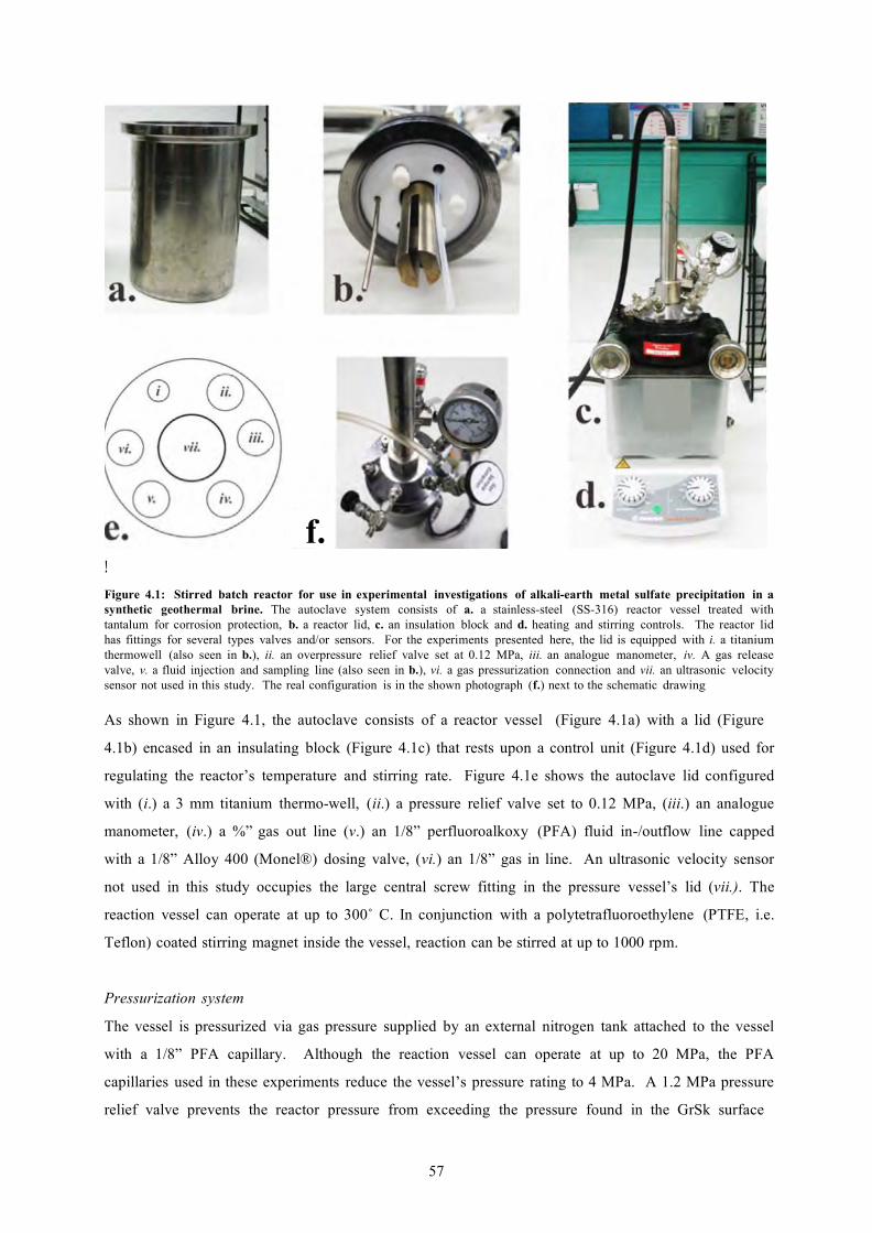
57

f. !

Figure 4.1: Stirred batch reactor for use in experimental investigations of alkali-earth metal sulfate precipitation in a synthetic geothermal brine. The autoclave system consists of a. a stainless-steel (SS-316) reactor vessel treated with tantalum for corrosion protection, b. a reactor lid, c. an insulation block and d. heating and stirring controls. The reactor lid has fittings for several types valves and/or sensors. For the experiments presented here, the lid is equipped with i. a titanium thermowell (also seen in b.), ii. an overpressure relief valve set at 0.12 MPa, iii. an analogue manometer, iv. A gas release valve, v. a fluid injection and sampling line (also seen in b.), vi. a gas pressurization connection and vii. an ultrasonic velocity sensor not used in this study. The real configuration is in the shown photograph (f.) next to the schematic drawing

As shown in Figure 4.1, the autoclave consists of a reactor vessel (Figure 4.1a) with a lid (Figure

4.1b) encased in an insulating block (Figure 4.1c) that rests upon a control unit (Figure 4.1d) used for

regulating the reactor’s temperature and stirring rate. Figure 4.1e shows the autoclave lid configured

with (i.) a 3 mm titanium thermo-well, (ii.) a pressure relief valve set to 0.12 MPa, (iii.) an analogue

manometer, (iv.) a %” gas out line (v.) an 1/8” perfluoroalkoxy (PFA) fluid in-/outflow line capped

with a 1/8” Alloy 400 (Monel®) dosing valve, (vi.) an 1/8” gas in line. An ultrasonic velocity sensor

not used in this study occupies the large central screw fitting in the pressure vessel’s lid (vii.). The

reaction vessel can operate at up to 300˚ C. In conjunction with a polytetrafluoroethylene (PTFE, i.e.

Teflon) coated stirring magnet inside the vessel, reaction can be stirred at up to 1000 rpm. Pressurization system

The vessel is pressurized via gas pressure supplied by an external nitrogen tank attached to the vessel

with a 1/8” PFA capillary. Although the reaction vessel can operate at up to 20 MPa, the PFA

capillaries used in these experiments reduce the vessel’s pressure rating to 4 MPa. A 1.2 MPa pressure

relief valve prevents the reactor pressure from exceeding the pressure found in the GrSk surface

58

installation during experimentation. Pressure can be manually released from the vessel by opening the

gas release valve on the reactors lid (Figure 4.1 e iii.). Fluid injection and sampling system

A single PFA capillary inserted to the bottom of the reaction vessel and terminating outside the vessel

with an 1/8” Alloy 400 (Monel®) dosing valve is used for both fluid injection and sampling (Figure

4.1e v.). For fluid injection, a second PFA capillary is filled with the volume of fluid to be injected.

One end of the capillary is attached to the dosing valve. The other end of the capillary is attached to a

pressurized nitrogen tank. The pressure in the injection line is then raised above 0.12 MPa, and the

dosing valve is opened. The overpressure in the injection line compared to the reaction vessel drives

the fluid in the injection line into the vessel, at which time the dosing valve is closed. Excess pressure

in the vessel caused by the injection is released as nitrogen gas through the pressure relief valve. To sample the fluid, a PFA capillary is used to connect the dosing valve to a polyetheretherketone

(PEEK) 50 mm membrane filter housing. Cellulose acetate (CA) filters with a pore size of 0.2 µm are

used in this study. The outflow from the filter housing leads to a 300 ml, PTFE-lined stainless steel

(SS-304) sampling cylinder. Once all parts are connected, sampling is performed simply by opening

the dosing valve and allowing the reaction vessel’s pressure to drive the experimental fluid through the

filter and into the sampling cylinder. The volume of the sampling cylinder is larger than that of the

reaction vessel, so there is no danger of the cylinder over-filling and, thus, driving sampled fluid back

into the vessel. 4.2.2.2 Experimental Solutions

Two different solutions are used in the experiments: a Na-Ba-Ca-Sr-Cl matrix solution and a Na2SO4

additive solution. The molal concentrations of the experimental fluids are reported in Table #4.4.

The matrix solution is designed to be representative of typical Ca-Na-Cl brines (e.g. Wolfgramm et al,

2004). The Ba concentration in the matrix is 5x higher than that found in the GrSk system. The extra

barium is added to ensure enough precipitate forms for proper analysis. The sulfate additive is

concentrated so that a small volume (i.e. < 2% of the matrix) of injected fluid will oversaturate the

matrix. Solutions are prepared using Merck brand analytical reagent grade salts. Salts used in the

matrix solution are NaCl, CaCl2 • 2H2O, SrCl2 • 6H2O, BaCl2 • 2H2O. The sulfate additive is prepared

with desiccated Na2SO4. Single distilled water (electrical conductivity = ~ 10 µS/cm) from the GFZ

Potsdam plumbing is used as the solvent. The solute masses are determined with a Sartorius®

analytical balance with an accuracy of ±0.1 mg. The solvent was weighed with a Mettler-Toledo®

precision balance with an accuracy of ±0.5% up to 5 kg. A stock solution of the matrix was made

using 2000 g of solvent. The sulfate additive was prepared with 500 g of solvent.

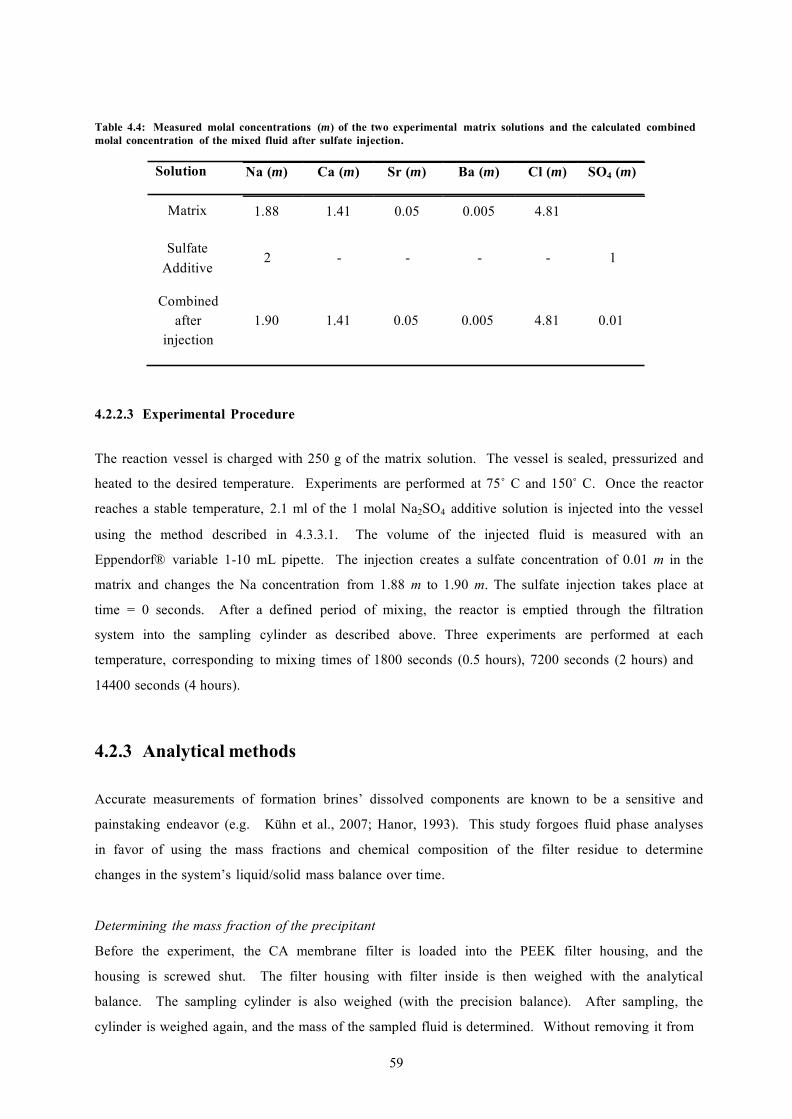
59

Na (m) Ca (m) Sr (m) Ba (m) Cl (m) SO4 (m)

1.88 1.41 0.05 0.005 4.81

2

-

-

-

-

1

Table 4.4: Measured molal concentrations (m) of the two experimental matrix solutions and the calculated combined molal concentration of the mixed fluid after sulfate injection.

Solution

Matrix

Sulfate Additive

Combined

after injection

1.90 1.41 0.05 0.005 4.81 0.01

4.2.2.3 Experimental Procedure

The reaction vessel is charged with 250 g of the matrix solution. The vessel is sealed, pressurized and

heated to the desired temperature. Experiments are performed at 75˚ C and 150˚ C. Once the reactor

reaches a stable temperature, 2.1 ml of the 1 molal Na2SO4 additive solution is injected into the vessel

using the method described in 4.3.3.1. The volume of the injected fluid is measured with an

Eppendorf® variable 1-10 mL pipette. The injection creates a sulfate concentration of 0.01 m in the

matrix and changes the Na concentration from 1.88 m to 1.90 m. The sulfate injection takes place at

time = 0 seconds. After a defined period of mixing, the reactor is emptied through the filtration

system into the sampling cylinder as described above. Three experiments are performed at each

temperature, corresponding to mixing times of 1800 seconds (0.5 hours), 7200 seconds (2 hours) and

14400 seconds (4 hours).

4.2.3 Analytical methods Accurate measurements of formation brines’ dissolved components are known to be a sensitive and

painstaking endeavor (e.g. Kühn et al., 2007; Hanor, 1993). This study forgoes fluid phase analyses

in favor of using the mass fractions and chemical composition of the filter residue to determine

changes in the system’s liquid/solid mass balance over time. Determining the mass fraction of the precipitant

Before the experiment, the CA membrane filter is loaded into the PEEK filter housing, and the

housing is screwed shut. The filter housing with filter inside is then weighed with the analytical

balance. The sampling cylinder is also weighed (with the precision balance). After sampling, the

cylinder is weighed again, and the mass of the sampled fluid is determined. Without removing it from

60

the filter housing, the filter is flushed profusely with distilled water to remove any soluble phases from

the filter residue. The entire unit is left to dry overnight at 105˚ C and is then re-weighed to determine

the mass of the filter residue. The mass fraction of the precipitant is equal to the mass of the filter

residue divided by the combined mass of the filter residue and the sampled fluid. Chemical analysis of the filter residue

The chemical composition of the filter residue is determined with a Panalytical® AxioMAX-Advanced

x-ray fluorescence (XRF) spectrum analyzer. The XRF analysis reveals the percent of each metal

oxide (e.g. CaO, SrO, BaO) contained in the analyzed powder. These oxide percentages are converted

to moles of precipitant / kg of experimental solution. Sulfur is not measured by the XRF. Because

one mole of sulfate precipitates per mole of cation in all of the sulfate minerals under investigation in

this study, total sulfate in the precipitant (in moles / kg solution) is assumed to be equal to the sum of

all moles of cation metal precipitants. Mineralogical analysis of the filter residue

The mineralogy of the filter residue was determined optically by analyzing gold-coated grain mounts

of the filter residue with a Carl Zeiss® EVO MA10 XVP scanning electron microscope (SEM)

equipped with EDAX® Genesis XM2 energy dispersive x-ray (EDX) spectrometer. Measurements

with the EDX analyzer are used as checks against the XRF analysis. The reactive surface areas of

growing crystals are also semi-quantitatively analyzed with the SEM. Estimated the filter residue’s specific reactive surface area

Combining visual analyses of a crystal’s morphology with the known density of the crystal’s

composition allows for rudimentary estimates of the filter residues’ specific reactive surface areas.

For example, suppose a precipitated barite crystal can be approximately described as a sphere with a

radius of 5 µm (a hypothetical supposition). Considering the volume (V) of the sphere to be:

(eq. 4.2) Vsphere = (4πr3)/3

and the surface area (SA) of the sphere to be

(eq. 4.3) SAsphere = (4πr2)

the hypothetical barite sphere has a V = ~524 µm3 and SA = ~314 µm2. Given a barite density of ~4.5,

the sphere of barite has a mass = [(524 µm3) * (4.48 g/1e12µm3)] = ~2.35 µg. Thus, the specific

reactive surface area (SSA) the barite sphere is ~314/2.35, or ~133 µm2/µg.

61

The SSA of the filter residue produced in the experiments presented herein are estimated by

performing this shape/density analysis on a representative crystal from the populations generated at

each time step and temperature. Standard state crystal densities are defined as 4.48 g/cm3, 2.98 g/cm3

and 3.97 g/cm3 for barite, anhydrite and celestite, respectively, as shown in the Table of Weights and

Measures (Appendix A). The volume and surface area of the selected crystal is estimated by the

describing the crystal’s dimensions in terms of the dimensions of the best fitting regular polygon.

4.2.4 Mass balancing and determining the kinetic rate law parameters

To determine a species’ dissolved concentration at any given time step, the moles of precipitant of that

species per kg of solution, as determined by the XRF data, is subtracted from the initial molal

concentration of that species in the experimental solution. Changes in dissolved concentrations over

time are used to determine a precipitation reaction order and a kinetic rate coefficient for each

precipitating mineral. This convention is used because, if mineral growth (as opposed removal of a

dissolved species) is used to monitor the reaction rate, the characteristic linear plots for 1st order

reactions (ln[A] vs. time) and 2nd order reactions (1/A vs. time) are indeterminate at t = 0, when the

initial amount of sulfate mineral is also = 0. The reaction order is determined by fitting the calculated dissolved concentration data to the

characteristic linear plot for a particular reaction order. The possibility of the alkali-earth metal sulfate

precipitation being a 0th – order reaction is ruled out, and data is not fitted to this linear equation. The

characteristic linear plots for 1st and 2nd order reactions are (ln[A] vs. time) and (1/[A] vs. time),

respectively. Whichever equation best fits the data to a line indicates the reaction order. The reaction

rate coefficient can then be gained directly from the fitted data. For a first order reaction, the rate

coefficient is the negative slope of the linear plot. For a second order reaction, the rate coefficient is

the slope of the linear plot. Results for all experiments are found below.

4.3 Results

4.3.1 Mass fractions and molal quantities of precipitants over time Total mass fractions of precipitants

Plots of the change in the precipitant’s mass fraction versus time are found for both temperatures (i.e.

75˚ C and 150˚ C) in Figure #4.2. At both temperatures, the accumulation of precipitants is described

well (r2 = .99 @ 75˚ C; r2 = .97 @ 150˚ C) by natural logarithmic functions. At 75˚ C, the filter residue

62

!#!!$"

Mas

s Fra

ctio

n mass per kilogram of solution ranges from ~1 g at t = 0.5 h to ~1.5 g at t = 4 h. At 150˚ C, the

precipitant’s mass per kg of solution ranges from ~0.8 g at t = 0.5 h to ~1.3 g at t = 4 h.

!#!!%"

!#!!$

!" !" &!!!" $!!!!" $&!!!"

!"#$%&'$()*+', 7Û & 75Û & !

Figure 4.2: Change in filter residue mass fractions versus time for sulfate precipitation kinetic experiments at 75˚ and 150˚ C.

Molal quantities of individual chemical species precipitated over time

A comparison of the molal quantities of Ca, Ba, Sr and SO4 precipitated over time at 75˚ C and 150˚ C

is shown in Figure 4.3. Moles of sulfate precipitated are calculated as the sum of all cation moles in

the precipitant. As is observed in the change in total precipitant mass fraction vs. time data (Figure

4.2), changes in molal quantities of precipitants vs. time are well described by natural logarithmic

functions for all chemical species at both temperatures. As is also observed in the overall precipitant

mass vs. time trend, precipitation proceeds faster at 75˚ C that at 150˚ C for all measured chemical

species. Whereas ~7 mM of sulfate minerals had formed after 4 hours at 75˚ C, only ~6 mM had

formed in the same time span at 150˚ C. The ratio of Ba:Sr:Ca in the precipitant remains constant throughout all times at ~ 0.58:0.30:0.12

during the experiment at 75˚ C. At 150˚ C, the Ba fraction is reduced to ~0.50. The smaller quantity

of Ba in the 150˚ C precipitants is accounted for predominantly by an increase in the Sr fraction to

~0.35. The Ca fraction of the cation moles at 150˚ C starts of high (0.15 @ t = 0.5 h) before

diminishing over time (0.11 @ t = 4 h).

63

!"#$

%&

%'()

'*+,

-./01

*2-.3

'%-)4

* !#!!'"

!#!!&"

!#!!%"

!#!!$"

!"

*+,-./0"

1.23+4"

*/256/3+4"

7.,83+4" !" (!!!" )!!!!" )(!!!"

5%,#*+2#$-)624* Û & Û & !

Figure 4.3: Moles of individual species precipitated per kilogram of synthetic geothermal brine versus time for kinetic experiments at 75˚ and 150˚ C.

Changes in molal concentrations of dissolved species over time

Initial molal concentrations of dissolved species in the experimental fluid are found in Table 4.4. The

initial dissolved calcium concentration is 1.41 mm. Considering significant figures, the dissolved

calcium concentration remains at 1.41 mm throughout the duration of the experiments at both

temperatures. The dissolved Ba concentration drops from a starting concentration of 5.0 mm to 1.1 mm

at t = 4 h (75˚ C) and 1.7 mm at t = 4 h (150˚ C). The Sr concentration drops from an initial value of

50 mm to ~48 mm after 4 h at both 75˚ C and 150˚ C. Considering the total change in the molal cation

concentrations to be equivalent to the molal change in SO4 concentration, dissolved SO4

concentrations decrease from an initial value of 10 mm to ~ 3.5 mm and ~3.7 mm after 4 h at 75˚ C and

150˚ C, respectively.

4.3.2 Fitting experimental data to the integrated rate laws’ linear form

The characteristic linear equations for 1st and 2nd order kinetic reactions are displayed in Table 4.3.

The possibility of sulfate precipitation proceeding as a 0th order reaction is eliminated, because 0th

order reactions refer primarily to radioactive decay, where the rate of the reaction is independent of the

64

reacting species’ concentration. Diagrams depicting the fitting of experimental data reported above to

these linear equations are shown in Figure 4.4-5 for experiments at 75˚ and 150˚ C, respectively. First order reactions

The coefficients of determination (r2) for Ca precipitation data fitted to the 1st order linear rate

equation are 0.46 and 0.52 for reactions at 75˚ C and 150˚ C, respectively. Strontium precipitation as a

1st order reaction fits the linear plot better than Ca, with an r2 = 0.59 at 75˚ C and r2 = 0.69 at 150˚ C.

Total sulfate fitted to the 1st order linear equations have r2 = 0.53 and 0.79 at 75 ˚ C and 150˚ C,

respectively. Changes in Ba concentration are fitted to the 1st order line with an r2 = 0.65 at 75˚ C and

r2 = 0.83 at 150˚ C. Second order reactions

The coefficients of determination for both Ca and Sr data fitted to characteristic 2nd order linear

equations are the same as for data fitted to the 1st order linear equations. The agreement of the Ba and

SO4 data with the 2nd order linear equations, however, is much stronger than their agreement with the

1st order equations. For Ba data, r2 = 0.81 at 75˚ C and r2 = 0.93 at 150˚ C. For total sulfate data, r2 =

0.77 at 75˚ C and r2 = 0.89 at 150 ˚ C.

Determining the reaction order and rate coefficient

At both temperatures, the characteristic linear plot for a 2nd order reaction best describes total sulfate

precipitation (i.e. all sulfate minerals combined). As shown in Table 4.3, the rate coefficient for a 2nd

order reaction is equal to the slope of the 2nd order linear rate plot. Thus, at 75˚ C, the reaction rate

coefficient for total sulfate precipitation is 0.014 kg of solution•mm-1•s-1, and at 150˚ C, the reaction

rate coefficient is 0.011 kg of solution•mm-1•s-1. The best overall data fit across all experiments is for

barium precipitation as a 2nd order reaction at both temperatures. The rate coefficient for barite is,

therefore, 0.0448 kg of solution•mm-1•s-1at 75˚ C and 0.0251 kg of solution•mm-1•s-1at 150˚ C. At both

temperatures, the barium r2 values are slightly better than the sulfate r2 values. Data fits are poor for

both calcium and strontium measurements.

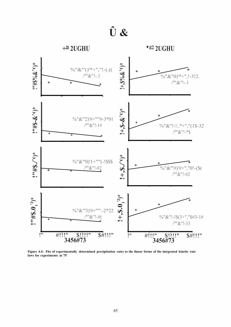
65

!"#$

.0 1 '2

)*

!"#$

./'( )*

!"

#$-&

'()*

!"#

$%&'

( )*

!+,$

.0 1 '2

)*

!+,$

./'( )*

!+

,$-&

'()*

!+

,$%&'

( )*

+38 2UGHU

Û &

'#7 2UGHU

%"&"'()'*+","!-(.(( /0"&"!-.1

%"&"'2)'#+"'"#-3*01 /0"&"!-1#

%"&"'0)'1+"'"(-!$$$ /0"&"!-#2

%"&"'3)'#+"'".-2*22

/0"&"!-#(

%"&"0)'*+",!-3!2. /0"&"!-.1

%"&"!-!..*+","(1$-32 /0"&"!-*$

%"&"'#)'#+","0!-($( /0"&"!-#2

%"&"!-!$(3+","$#3-1#

/0"&"!-33

!" #!!!" $!!!!" $#!!!" 3456#73

!" #!!!" $!!!!" $#!!!" 3456#73

Figure 4.4: Fits of experimentally determined precipitation rates to the linear forms of the integrated kinetic rate laws for experiments at 75˚

66

(OQ>

62 * !+

()

(OQ>

6U!'

()

(OQ>

%D!'

()

(OQ>

&D!'

()

(li>

62 * !+

()

(li>6

U!'

()

(li>%

D!' ()

(li

>&D!

' ()

$%& 2UGHU

lS Û &

!"# 2UGHU

%"&"'()'*+","!-(.(. /0"&"!-#0

%"&"'1)'#+"'"#-#0#( /0"&"!-*(

%"&"'()'2+"'"(-!!3. /0"&"!-23

%"&"'2)'#+"'".-*.!* /0"&"!-13

!" #!!!" $!!!!" $#!!!" VHFRQGV

%"&"'0)'*+",!-1!3. /0"&"!-#0

%"&"!-!0#$+","0#0-$3 /0"&"!-3(

%"&"'#)'#+","0!-012 /0"&"!-1!

%"&"!-!$$+","$0*-1$ /0"&"!-*3

!" #!!!" $!!!!" $#!!!" VHFRQGV

Figure 4.5: Fits of experimentally determined precipitation rates to the linear forms of the integrated kinetic rate laws for experiments at 150˚ C.

67

4.3.3 Filter residue analysis with scanning electron microscopy

4.3.3.1 Mineralogical and chemical composition of the filter residue

Scanning electron photo-micrographs, along with accompanying EDX chemical analyses, for the 75˚

C experiments are shown in Figure 4.6. For all time steps at 75˚ C, all three cations are incorporated

into a single precipitating phase. Based on previous experience with SEM analyses of sulfate

precipitants (see appendix) and literature reports on barite crystal growth (e.g. Pina et al., 1998;

Bosbach et al., 1998; Archibald et al., 1996; Christy and Putnis, 1993), the solid phase is identified

visually identified as barite. Analyses performed with the EDX on the general mass of precipitants

and on individual crystals within the populations confirm the predominance of Ba in the crystals, with

Ca and Sr appearing as accessory phases. The EDX shows a generally higher concentration of Ba in

the solid (~68% of cations) than the XRF (~57% of cations). The EDX also shows a slight decrease in

the Ba:Sr ratio over time, a result contrary to the XRF data showing a stable Ba:Sr ratio with time.

The extra Ba measured by the EDX compared to the XRF is compensated for by a lower Ca

measurement. For the 75˚ C experiments, Ca only accounts for ~4% of the total cation composition,

according to the EDX measurements. SEM photographs, with accompanying EDX analyses results

for the experiments at 150˚ C, are shown in Figure 4.7. Similar to the 75˚ C results, all cations at 150˚

C are precipitated in a single crystalline phase. There is no trend in the concentration of any cation

species with time at 150˚ C, but the EDX measurements at 150˚ C are generally similar to those made

at 75˚ C. As is the case with XRF measurement, the EDX measures slightly less Ba at 150˚ C than at

75˚ C.

4.3.3.2 Crystal growth

A selection of images designed to show the evolution of the filter residues’ crystal morphology is

shown in Figure 4.8 for experiments at 75˚ C and Figure 4.9 for experiments at 150˚ C. Initial

precipitants at 75˚ C nucleate as twinned, bladed to platy subhedral crystals growing stacked on top of

each other. By 0.5 h, the nuclei begin to aggregate, either as flattened spheroids or as sub-rectangular

prisms radiating around and through a tabular center. The spheroids have diameters ranging from ~2

– 4 µm (Figure 4.6), and the prisms are roughly ~2 x 0.25 x 0.1 µm in dimension (Figure 4.8). By 2 h,

all of the twinned crystals evolve into either the spheroids or the radially symmetrical aggregates of

prisms. The average diameter of the spheroids increases to ~5 µm (Figure 4.6). The rectangular

prisms observed after 0.5 h begin to grow toward trapezoidal termini in the elongated direction after 2

h. The dimensions of the prisms are now ~ 3 x 1.2 x 0.25 µm. By 4 h, many of the spheroids have

undergone a transformation to aggregates of tabular to platy, now euhedral crystals (Figure 4.6 & 4.8).

At 4h, the platy-prismatic crystals have grown to dimensions of ~ 4 x 2 x 0.25 µm.

68

Cat

ion

%

Cat

ion

%

0.5 h

2 h

4 h

100%

Û &

100%

80% 80%

60% 60%

40% 40%

20% 20%

0% 0.5 h 2 h 4 h

Ba

0% 0.5 h 2 h 4 h

Sr Ca

Figure 4.6: Visual overview and EDX analysis of alkali-earth metal sulfate precipitants after 0.5, 2 and 4 hours at 75˚ C. Only barite crystals formed, with Sr and Ca being incorporated into the barite in the ratios denoted by the EDX analysis. The EDX percentages on the left are for the whole population of crystals. The graphs on the right correspond to the individual crystals depicted above.

69

Cat

ion

%

Cat

ion

%

0.5 h

2 h

4 h

100%

lS Û &

100%

80% 80%

60% 60%

40% 40%

20% 20%

0% 0.5 h 2 h 4 h

Ba

0% 0.5 h 2 h 4 h

Sr Ca

Figure 4.7: Visual overview and EDX analysis of alkali-earth metal sulfate precipitants after 0.5, 2 and 4 hours at 150˚ C. Only barite crystals formed, with Sr and Ca being incorporated into the barite in the ratios denoted by the EDX analysis. The EDX percentages on the left are for the whole population of crystals. The graphs on the right correspond to the individual crystals depicted above.

70

Û &

!"#$% &'()*+,('$-./01)*$'+2(30+4305

!"#$%$&"!#$%$&"'$() 6./01)*$74*82(

&"&*!#$()+

6./01)*$9)005 &"!,$-.

6./01)*$:8.;)-($<.()5 '",&$()!

:=(-+;+-$>()-1+?($:8.;)-($<.()5 *"/+$()!0-.

@$%

&'()*+,('$-./01)*$'+2(30+4305 +$%$'"!$%$"!#$() 6./01)*$74*82(5

&"1$()+

6./01)*$9)005 /"&+$-.

6./01)*$:8.;)-($<.()5 1"+$()!

:=(-+;+-$>()-1+?($:8.;)-($<.()5 !"+'$()!0-.

A$%

&'()*+,('$-./01)*$'+2(30+4305

/"#$%$!$%$&"!#$() 6./01)*$74*82(5

!"!#$()+

6./01)*$9)005 '&$-.

6./01)*$:8.;)-($<.()5 !'"!#$()!

:=(-+;+-$>()-1+?($:8.;)-($<.()5 !"'+$()!0-.

!

Figure 4.8: Evolution of crystal morphology and estimates of specific reactive surface for strontio -barite crystals precipitating after 0.5, 2 and 4 hours at 75˚ C.

71

lS Û &

0.5 h Idealized crystal dimensions:

4.7 x 2.1 x 0.25 µm Crystal Volume:

2.47µm3

Crystal Mass: 11 ng

Crystal Surface Area: 23.14 µm2

Specific Reactive Surface Area: 2.1 µm2/ng

2 h

Idealized crystal dimensions:

6.5 x 3 x 0.4 µm Crystal Volume:

7.8 µm3

Crystal Mass: 35 ng

Crystal Surface Area: 46.6 µm2

Specific Reactive Surface Area: 1.33 µm2/ng

4 h

Idealized crystal dimensions:

7 x 3.2 x 0.4 µm Crystal Volume:

8.96 µm3

Crystal Mass: 40 ng

Crystal Surface Area: 50 µm2

Specific Reactive Surface Area: 1.25 µm2/ng

Figure 4.9: Evolution of crystal morphology and estimates of specific reactive surface for strontio-barite crystals precipitating after 0.5, 2 and 4 hours at 150˚ C.

72

Crystals precipitated at 150˚ C, as shown in Figure 4.9, are larger and better developed than those

precipitating at 75˚ C. The crystal populations at 150˚ C after 0.5 h consists of euhedral, strontio-

barite plates appearing individually, or as aggregates with radial symmetry, much like the paddle of a

riverboat. The plates are ~4.5 µm long by ~2 µm wide and can also aggregate into ~4.5 µm diameter

balls. After 2 hours, the plates become larger and now have dimensions of ~6 x 3 x 0.25 µm. The

number of spoke-shaped aggregates is reduced; as the crystals continue to grow, they evolve from

clumps of many individual crystals to the larger euhedral crystals. By 4 h, nearly all of the crystals

evolve from the radiating aggregate stage to the platy stage. The dimensions of the crystal plates

observed after 4 h of growth at 150˚ C are ~7 x 3 x 0.4 µm. 4.3.3.3 Estimating changes in specific reactive surface area.

Crystals used for estimating the specific reactive surface area (SSA) of the filter residue are shown in

Figure 4.8 and Figure 4.9 for 75˚ C and 150˚ C experiments, respectively. The relevant parameters for

calculating the SSAs and the results of the calculations are shown therein. At both temperatures, the

SSA of the representative crystals decreases with time. For the 75˚ C reaction, the SSA ranges from

~6.4 µm2/ng at t = 0.5 to ~2.1 µm2/ng at t = 4 h. During the same time span, the SSA for

representative crystals at 150˚ C ranges from ~2.1 µm2/ng to ~1.25 µm2/ng.

4.4 Discussion

4.4.1 Effects of temperature on reaction rate and stable phase assemblage Chemical analyses of minerals precipitated from a sulfate-oversaturated, mixed chloride salt solution

show that barite is the dominant scale-forming mineral at (T, p, x) conditions analogous to those found

in low-enthalpy geothermal fluids produced from sedimentary basins. On a molar basis, Ba comprises

nearly 60% of the cation fraction of the precipitant formed at 75˚ C and more than half of the cation

fraction of the precipitant formed at 150˚ C. The remainder of the cation fraction is split between Sr

and Ca in the ratio of ~2:1. No growth of anhydrite or celestite was observed with the SEM, although

the EDX spectra detected both of the elements in the barite crystals. The absence of these minerals in

the filter residue supports the conclusions of Kühn et al. (1997), who performed barite

precipitation/dissolution experiments in a chemical system similar to the one employed in this study

and who also report the absence of anhydrite and celestite in the precipitant.

73

Applying the method of integrated rates (4.2.1, above) to the experimental data reveals the behavior of

the oversaturated solution during the 4 hours of experimentation to be best described by a 2nd order

barite precipitation reaction, with a rate coefficients of 0.0448 kg of solution•mm-1•s-1at 75˚ C and

0.0251 kg of solution•mm-1•s-1at 150˚ C. These values represent significantly faster reactions than the

ones reported by Kühn et al. (1997). Kühn et al. (1997) used a Ba concentration ~100x less than the

concentrations used in this study and suggested greater degrees of super-saturation may require

different rate coefficients. The Ba concentration of the GrSk fluid is between that used by Kühn et al.

(1997) and that used in this study. Kühn et al.’s (2007) experiments also differed from the

experiments presented here in that they were only performed at atmospheric conditions. The reaction

order reported here is in agreement with that reported by Christy and Putnis (1993), but the rate

coefficients determined by these experiments differ from that Christy and Putnis (1993) by ~3 orders

of magnitude. Although these authors studied barite precipitation at up to 85˚ C, they only employed

background ionic strengths of < 0.1 M. Christy and Putnis (1993), therefore, warned that higher

salinities might render their rate constant calculations invalid. The study presented here is the first to

present a complete kinetic rate law for barite precipitation from a synthetic geothermal brine at

conditions analogous to those found in a working power plant. While the Arrhenius equation predicts that the precipitation reactions should progress faster at higher

temperatures, this effect is observed neither in the mass fractions nor the chemical composition of the

filter residues studied at the two temperatures. On the contrary, sulfate precipitation in the synthetic

geothermal brine used in this study occurred faster at the lower temperature, demonstrating that the

precipitation rate is controlled more by the degree of oversaturation than by the temperature. This

information is useful to geothermal plant operators because it reinforces the idea that barite scale will

tend to form on the cold side of the heat exchanger. If only the temperature governed the reaction

kinetics, more precipitant would be expected on the hot side of the heat exchanger. Because Ba has

less competition from Ca at 75˚ C than at 150˚ C, however, the Ba is able to bond more easily with the

SO4 at 75˚ C, and, thus, barite should accumulate faster on the cold side of the heat exchanger. The

phase assemblage diagrams presented in Chapter 3 of this work (Figure 3.3) support this hypothesis by

showing a larger barite stability field at 75˚ C than at 150˚ C. The phase assemblage diagram in

Figure 3.3 also predicts the absence of anhydrite and celestite in the precipitant. The synthetic

geothermal brine used in this study would plot squarely in the barite stability field in these diagrams at

both temperatures.

4.4.2 Evolution and mechanisms of crystal growth

Precipitant evolution over the 4-hour time span of the reaction follows similar trends at 75˚ C and 150˚

C. Crystal growth at both temperatures appears to follow the classic Ostwald ripening model of

74

crystal growth (e.g. Steefel and Van Cappellen 1990; Morse and Casey, 1988), in which molecules

bound in relatively unstable arrangements continuously rearrange to form progressively more stable

arrangements. This phenomenon can be readily observed in the SSA of the evolving crystals, which

continually decrease with increased growth. The lower the SSA, the more stable the crystal is. The crystals produced in these experiments exhibit initial growth similar to that described in several

previous studies (e.g. Kowacz et al., 2007; Bosbach et al., 1998; Pina et al., 1998), in which growth

occurs with a distinct cross section parallel to the [001] crystallographic axis (e.g. Figure 4.8, 0.5 h). A

succession of twins appears to grow in radial symmetry around the center of the initial crystal, until,

by 0.5 h, most of the particles are spherical to cylindrical aggregates of twinned crystals grown either

in rotation or screw-steps around the nucleus. The estimated SSA of the precipitant at this point

(~6.43 µm2/ng) is relatively high compared the estimated SSA at 4 h (2.13 µm2/ng). The first SSA

(i.e. at t = 0.5 h) is indicative of a highly charged (i.e. reactive) particle that gradually re-forms (i.e.

grows) into more stable crystals. The stable crystals have less SSA for free ions to bind to; therefore,

the reaction rate slows down as the reaction progresses towards equilibrium. The Ostwalt ripening is also observed visually in the morphology of the crystals precipitated at 75˚ C.

Over the span of the experiment, individual crystals comprising the spherical aggregates evolve from a

thin, acicular to bladed habit to more a tabular or prismatic habit (Figure 4.6). Furthermore, some of

the spherical aggregates appear to evolve into singular platy crystals (e.g. Figure 4.8), a step that

significantly reduces the precipitants SSA. At 150˚ C, however, the ripening is not as visually evident

as it is at 75˚ C. At the elevated temperature, the nucleation of spindly crystal aggregates and their

growth to larger, more stable forms is not observed. Rather, crystals formed at 150˚ C are already

subhedral plates by t = 0.5 h. The SSA of the crystals formed at 150˚ C are also lower than for those

formed at 75˚ C for all time intervals. These results suggest that, although crystal growth is more

massive at 75˚ C than 150˚ C, the nucleation/growth/ripening process is faster at the higher

temperature than observed at 75˚ C. This explanation reconciles the discrepancy between observed

crystal growth and the behavior predicted by the Arrhenius equation, as discussed above (4.4.1)

4.5 Conclusions

Kinetic rate laws for alkali earth metal sulfate precipitation from a synthetic geothermal brine are

successfully determined with the method of integral rates for solutions reacting at 75˚ C and 150˚ C.

At 75˚ C, the rate law for total sulfate precipitation is written as {rate = 0.0137*[SO42-]2}. At 150˚ C,

the rate law for total sulfate precipitation is written as {rate = 0.011*[SO42-]2}. If just barite

precipitation is considered, the rate coefficients become 0.045 and 0.025 at 75˚ C and 150˚ C,

75

respectively. The units for the second order rate coefficient in this study are (kg of solution•mm-1•s-1).

The precipitants’ SSA is estimated for each time step and temperature and is shown to decrease as

precipitation continues. The (1) the reaction order, (2) the rate coefficient and (3) the change in SSA

over time are the three parameters required to develop a kinetic model of mineral precipitation in the

GrSk plant.

76

5. 1-D reactive transport models of alkali earth metal sulfate scaling risks in the

Groß Schönebeck in-situ geothermal laboratory

77

{ 5.1 Introduction The location, extent and composition of alkali earth metal sulfate precipitation in the GrSk surface

infrastructure can be predicted by incorporating the kinetic parameters experimentally determined in

Chapter 4 into a reactive-transport model. Reactive transport models, which couple transport

calculations with chemical reaction simulations, are commonly used to predicted mass, heat and fluid

transfer in geologic systems (e.g. Bethke, 2008; Steefel et al., 2005; Steefel and Lasaga, 1994; Yeh

and Tripathi, 1989). A series of 1D reactive transport models, detailing precipitation from produced

brine at various stretches in the GrSk geothermal loop, is presented in this Chapter. Frick et al. (2011) describe in some detail the GrSk power plant infrastructure. Many of the details

presented below are based on personal correspondence with these authors. A schematic drawing of

the GrSk surface infrastructure is seen in Figure 5.1. For the purposes of this study, the surface

infrastructure is arbitrarily defined as the flow path from the production pump to the heat exchanger

and down the injection well to a depth equivalent to that of the production pump. The pump is

situation in well GrSk 04/05 at a ~1200 m depth (Frick et al., 2011). The heat exchanger is located

~100 m from both the production and injection wellheads, making the total length of the surface

infrastructure under investigation ~2600 m. Fluid is transported throughout the power plant in DN 100

(100 mm ø) pipes. The total volume of the surface infrastructure, not including the negligible volume

of the heat exchanger, is, therefore, ~20 m3.

Thermal Fluid In (from 1200 m depth)

Working Fluid In (from ORC)

Working Fluid Out (to ORC)

Thermal Fluid Out (to 1200 m depth)

h

Model 1: Production w well to heat exchanger

d

Model 2: Through one set

of exchanger plates

(h) x (w) x (d)

~2 m x ~1 m x 0.003 m

Model 3: Complete surface infrastructure

Figure 5.1: Schematic drawing of the Groß Schönebeck surface infrastructure, with a close up of the heat exchanger plate configuration.

78

As show in Figure 5.1, the primary side of the GrSk heat exchanger (i.e. the side transporting

geothermal brine and not the coolant fluid) consists of 155 pairs of titanium plates. Plates are

separated from one another by a ~ 3 mm flow space. The plates themselves are ~ 2 x 1 m in area.

Thus, the volume of brine contained between a pair of heat exchanger plates is ~0.006 m3, and the total

volume of the heat exchanger is ~ 0.9 m3. The heat exchanger’s inlet temperature is ~150˚ C, and the

outflow temperature is ~75˚ C.

5.2 Model Descriptions The X1t program in the GWB is used as the modeling software. All models use the thermo_pitzer

database. Three different scenarios in the GrSk surface infrastructure are modeled. In the first

scenario, reactive transport phenomena are calculated in the segment from the production well’s pump

to the heat exchanger’s inlet. The second modeled scenario considers the reactive transport behavior

between two individual plates in the heat exchanger. The third scenario considers the entire pathway

in the GrSk surface infrastructure, from the production pump, across the heat exchanger and down the

injection well to a depth equal to the depth of the production pump (~1200 m). The areas in which

reactive transport phenomena are modeled are marked on Figure 5.1.

Inputs for ionic concentrations in all three reactive transport models are the same as for the

equilibrium model presented in Chapter 3 (Table 3.1). Kinetic parameters determined in Chapter 4 of

this study are converted to the GWB’s input units for kinetic reactants. The required parameters are (1)

an initial starting mass, (2) the specific surface area (SSA) of the initial starting mass, (3) a reaction

order and (4) a rate constant with units of mol/cm2•s. The first three values are taken directly from the

Chapter 4 results, while the new rate constant must be recalculated from the results. Parameters for

individual minerals (barite, anhydrite and celestite) are determined by multiplying the parameters’

values taken for the idealized crystals analyzed in Chapter 4 (Figure 4.8-9) by the percentages of the

cations comprising the idealized crystal, as measured by the EDX (Figures 4.6-7). A summary of these

kinetic parameters is found in Table 5.1

Preliminary testing of the GWB’s reactive transport modeling features performed within the context of

this study show that varying the flow rates between 25-75 m3/h have negligible effects on the mass, composition or location of precipitants determined by the model calculations. The results presented

below, therefore, consider only a volumetric flow rate of 50 m3/h, which is indicative of the flow rate

required for economic energy production in the GrSk system (Hurter, 2002). The linear flow rate

required by the 1-D model is calculated by dividing 50 m3/h by the cross sectional area of the vessel in

which the fluid is transported. For flow through the heat exchanger, this area is ~0.003 m2. For flow

through the plant’s main piping, the area is ~0.008 m2 (Figure 5.1). To represent flow in an open

79

BaSO4 CaSO4 SrSO4 BaSO4 CaSO4 SrSO4 BaSO4 CaSO4 SrSO4

7.70E-

4.40E-

2.86E-

7.70E-

4.40E-

2.86E

7.70E-

4.40E-

2.86E- 09 10 09 09 10 -09 09 10 09

3.30E-

3.23E-

1.56E-

3.30E-

3.23E-

1.56E

3.30E-

3.23E-

1.56E- 11 12 11 11 12 -11 11 12 11

1.62E-

9.26E-

6.02E-

1.62E-

9.26E-

6.02E

1.62E-

9.26E-

6.02E-

07 09 08 07 09 -08 07 09 08

1.13E-

1.94E-

1.44E-

7.51E-

1.29E-

9.54E

1.13E-

1.94E-

1.44E-

07 07 07 08 07 -08 07 07 07

channel, the initial porosity is set to 100%, and the boundary conditions are set to constant flow. Flow

rates for the various models are summarized in Table 5.2.

Table 5.1: Kinetic parameters incorporated into the GrSk reactive transport models

Model #1 Model #2 Model #3

Kinetic Parameters

Mineral starting mass

(g)

Mineral starting moles

Mineral

surface area (cm2)

Pump to Heat Exchanger

Between Heat Exchanger Plates

Entire Surface Infrastructure

GWB rate constant

(mol/cm2•sec)

The ~1300 m distance between the production pump and the heat exchanger is represented in the first

modeling scenario by 130 nodes of 10 m finite elements. Based on a 100 mm pipe diameter, the total

volume of the system is ~10 m3, and the fluid residence time at the given flow rate is 11.5 minutes.

The inlet temperature and the temperatures at all nodes are held constant at 150˚ C. The linear flow

rate is 1.7 m/s. Model parameters for flow between the production pump and the heat exchanger are

shown in Table 5.2. Changes in the precipitants’ mass, composition and location along the transport

route are measured at intervals over a two-hour time span, which is the longest time span in which the

calculations converged to a solution, under the given boundary conditions.

As shown in Figure 5.1, above, the dimensions of the heat exchanger plates are ~2 x 1 m, and the

distance between two plates is ~0.003 m. These dimensions are represented in the model by 40 nodes

of 0.05 m finite elements with a volume of ~0.006 m3 and a linear flow rate of ~4.6 m/s. Thus, the

residence time of the fluid between two heat exchanger plates is ~5 s. The temperature drop in the

heat exchanger is modeled by assigning each of the model’s 40 nodes with a discrete temperature

value, decreasing linearly from T = 150˚ C at node = 0 to T = 75˚ C at node = 39. The inlet fluid

temperature is set to 150˚ C. To prevent the hot inlet fluid from raising the temperature on the cold

end of the heat exchanger, the model is run in fixed temperature mode, considering reactive transport

behavior at intervals over the span of one hour. As is the case with the 2 h simulation in the previous

model, 1 h was the longest time period in which a solution could be converged upon. Table 5.2

displays the modeling parameters for fluid flow through the GrSk heat exchanger.

80

Table 5.2: Summary of physical parameters used for reactive transport modeling of the GrSk surface infrastructure.

Model #1 Model #2 Model #3 Physical Pump to Heat Between Heat Entire Surface

Parameters Exchanger Exchanger Plates Infrastructure

Length 1300 m 2 m 2600 m

Nodes 130 x 10 m 40 x .05 cm 14 x ~186 m

Temperature 150˚ C 150˚ - 75˚ C 150˚ - 75˚ C

Flow Rate 1.7 m/s 4.6 m/s 1.7 m/s

Residence

Time 11.5 minutes 5 seconds 25 minutes

Porosity 1 1 1

Boundaries constant flow constant flow constant flow

The entire GrSk infrastructure is modeled as a 2600 m length consisting of 14 nodes of 185.7 m finite

elements, with the temperature at nodes 0-6 fixed at 150˚ C and nodes 7-13 fixed at 75˚ C. The inlet

fluid temperature is 150˚ C. The system’s total volume, linear flow rate and fluid residence time are

~20 m3, 1.7 m/s and ~25 minutes, respectively, all of which are summarized in Table 5.2. For the

entire surface infrastructure model, the longest time period at which calculations in the GWB converge

upon a solution is 5 days. Boundary conditions for this model are also displayed in Table 5.2.

5.3 Results & Discussion

5.3.1 Flow from the production pump to the heat exchanger

The residence time of fluid produced at 50 m3/h in a 100 mm ø length of pipe from the GrSk

production pump to the inlet of the heat exchanger is about 11.5 minutes. As shown in Figure 5.2,

there is no change in the free volume within the pipe during this time, i.e. the pore fraction remains 1.

As is also shown in Figure 5.2, the total amount of sulfate precipitant formed in this timeframe is ~4

mg per m3 of brine. A model considering simply a time-step progression of individual residence times

predicts no risk of scaling-induced pipe volume reduction over time during operation of the plant. In

such a scenario, mineral precipitants would still accumulate in the plant’s filters at the rate of ~25 mg

per m3 of brine per hour.

81

solid mass (g/m

3of brine) fr

ee v

olum

e fr

actio

n

1.2

1.0

Pump to heat exchanger residence time - 11.5 minutes

0.01

0.8

0.6

0.4

0.2

0.0 0.001 0 325 650 975 1300

distance along flow path (m) solid mass free volume fraction

Figure 5.2: Pipe free volume fraction and precipitated solid mass as a function of distance between the GrSk production pump and heat exchanger after 1 fluid residence time (~11.5 minutes) at a flow rate of 50 m3/h.

Figure 5.3 shows the total decrease in free volume within the pipe and the total mass of precipitant

formed if the system is modeled over a two-hour production interval. The GWB failed to converge to

a solution for time periods longer than this. Loss of free volume coincides with the onset of

precipitation after about 40 minutes of production. After two hours, over 2 g of precipitant have

formed per m3 of brine produced, reducing the pore fraction from 1 to ~0.6. The location of the pore-

fraction reduction along the production line and chemical composition of the precipitants are shown in

Figure 5.4. Precipitation is predicted only within the first 15-20 m of the 1300 m length considered in

this model. Whereas the precipitated mass is distributed evenly over the 15-20 m after one hour, after

2 hours the mass shows clear preference for forming in the upstream direction. The precipitation rate

is linear for the first 0.5 hours, before slowing down between 0.5 and 2 hours. The decrease in the

precipitation rate is congruent with that predicted by the second order reaction kinetics determined in

Chapter 4 of this work.

The mass of precipitant predicted by this model after 2 hours of production at 50 m3/h is ~200g. This

amount is equivalent to ~2 g/m3 of produced brine. The mass fraction of insoluble solids determined

in the field (Chapter 2.3.2) averages about 300 g/m3. The extent to which barite comprise these solids is unknown; insufficient material was produced during the mass fraction experiments for chemical

analyses. According to the XRF analyses performed on the GrSk filter residue (which included

soluble and insoluble phases) the filter residue consists of ~0.5% - 7% BaSO4. Thus, ~2 - 25 g/m3 of

barite may have been in the filter residue measured in the insoluble mass fraction experiments (2.3.2).

82

solid mass (g/m

3of brine) fr

ee v

olum

e fr

actio

n On the low end of the this estimate, the model is in excellent agreement with value calculated from the

field data, but field calculations can be up to 10x higher than the modeled calculations. It would

appear, therefore, that the model underestimates the amount of precipitant actually found in the GrSk

system.

1.2

1

0.8

0.6

0.4

0.2

2.5

2

1.5

1

0.5

0 0 0 20 40 60 80 100 120

time (m)

solid mass

free volume fraction

Figure 5.3: Change in pore fraction and solid mass precipitated between the GrSk production pump and heat exchanger during 2 hours of production at 50 m3/h.

Both barite and anhydrite are predicted to precipitate between the production pump and the heat

exchanger. Celestite is not expected to precipitate in any significant amounts. The ratio of barite to

anhydrite (Ba:Ca ratio) in the precipitant, as shown in Figure 5.4, increases linearly from an initial

value of ~20:1 to ~200:1 after 15 minutes. These ratios are constant at each time step across the entire

flow length from the production pump to the heat exchanger. By 30 minutes, the Ba:Ca ratio increases

sharply to ~9000:1 in the first ~1% of the flow length, before decreasing exponentially to a stable

value of ~100:1 over the last 1000 m of pipe. By 2 hours, the Ba:Ca ratio in the precipitant mass drops

to ~1:10, indicating the onset of anhydrite precipitation between 30 and 120 minutes. As is the case at

30 minutes, at 2 hours there is a sharp increase in the Ba:Ca ratio at the very beginning of flow path,

but the spike is not as pronounced as it is after 30 minutes. The spike in Ba concentration at the

beginning of the path shows clearly (Figure 5.4) that barite is the first forming mineral in the system,

but barite precipitation trails off in favor of anhydrite within the first ~500 m of the flow path between

the production well and the heat exchanger.

83

free

vol

ume

frac

tion

Ba

: Ca

Rat

io

solid

mas

s (g

/m3 of

brin

e)

cm fr

om p

ipe

wal

l

a. Distance along flow path (m)

1.0

0 325 650 975 1300

0.8 0

0.6

0.4

0.2

2.5

5

2.5

0

Free volume change in a 100mm ø pipe

0 1 2 3 4 5 6 7 8 9 10 11 12 13 14 15

distance along flow path (m) 0.0

b. 10

1 h 2 h

1E-3

1E-7

1E-11

c. 1E4

0 260 520 780 1040 1300 Distance along flow path (m)

1 min 5 min 15 min 30 min 2 h

1E2

1E0

1E-2

0 260 520 780 1040 1300

Distance along flow path (m)

1 min

5 min

15 min

30 min 2 h

Figure 5.4: Location, extent and composition of precipitation between the GrSk production pump and heat exchanger after 2 hours of production at 50 m3/h. a. location of porosity reduction along the flow path, with a close-up of the 1st 15 m of piping. b. accumulation of solid mass as a function of time (gray scaling) and distance along the production stretch (x-axis) and c. ration of barite to anhydrite as a function of time (size of hyphenation) and distance along the production stretch (x- axis).

84

The reactive transport model of brine production from the GrSk production pump to the heat

exchanger shows an initial period of barite growth within the immediate vicinity of the pump that

gradually extends to a distance of ~15-20 m along the production well over a 2-hour timespan. The

model’s prediction is proved accurate by the study of Holl et al. (2003), wherein barite precipitation on

the pump is reported. The initial predominance of barite precipitation is gradually reduced after ~30

minutes of production, when anhydrite becomes the major precipitating phase. This prediction has not

been verified by any field reports of anhydrite precipitants, although the XRF studies of GrSk filter

residue presented in Chapter 2 of this work do show the presence of up to 20% Ca in the precipitants.

The results of this model suggest that alkali-earth metal sulfate scaling is a hazard in the production

well. The reaction kinetics determined in Chapter 4 of this work, combined with the flow parameters

found at the GrSk site, predict that most of the dissolved SO4 will be consumed in a precipitation

reaction before the fluid reaches the heat exchanger.

5.3.2 Flow within the heat exchanger At a production rate of 50 m3/h, the residence time of fluid traveling between two heat exchanger

plates is ~5 s. Modeled results for the change in the system’s free pipe volume and solid phase mass

over this time interval are shown in Figure 5.5. No change in the pipe volume is observed after 1 fluid

residence time, and the solid mass is on the order of 0.01 – 0.1 mg/m3 of produced brine. This amount

of precipitated mass is ~100x less than that predicted after 1 fluid residence time in the previous model

(5.3.1), and suggests that up 5 mg/h of alkali earth metal sulfates may be pumped back down the

injection well. Similar to the results from the previous model, considering the behavior of the fluid

simply as a progression of individual residence times suggests no immanent scaling risks. When the

system is modeled over time, however, the free volume between the heat exchanger plates first

becomes reduced after ~35 minutes, coinciding with the onset of precipitation. The GWB failed to

coverage a solution for simulations longer than 1 hour.

Results for the accumulation of precipitated mass and the concomitant decrease in the system’s free

volume between the heat exchanger plates over time are plotted in Figure 5.6. The precipitant’s total

mass increases exponentially from ~0 at the start of the simulation to more than 4 g/m3 of produced

brine after 60 minutes. The exponential growth is characteristic of the 2nd order reaction precipitation

reaction predicted in Chapter 4. The amount of precipitant is roughly twice as much as the amount

predicted in the previous model, yet only in the half the amount time. Precipitation calculated by the

model leads to a decrease in the system’s free volume to < 50% by t = 60 minutes. The larger

reduction in free volume in the heat exchanger model compared to the previous model is due to both

the smaller volume between the heat exchanger plates (compared to the 100 mm ø pipes) and the faster

linear flow rate through the plates in comparison with the previous model. A faster linear flow rate

85

solid mass (g/m

3of brine) solid m

ass (g/m3of brine)

free

vol

ume

frac

tion

free

vol

ume

frac

tion

means more fluid passing through the system and, hence, more precipitant in any given time period. It

must be noted however, that the rate at which free volume between the heat exchanger is reduced is

applicable only if precipitated materials are not removed from the system, i.e. filtered out or pumped

further down the injection well.

1.2

1

Between heat exchanger plates residence time = 5 seconds

1E-4

0.8

0.6

0.4

0.2

0 1E-5 0 50 100 150 200

distance along flow path (m) solid mass free volume fraction

Figure 5.5: Pore fraction and precipitated solid mass as function of distance between two plates in the GrSk heat exchanger after 1 fluid residence time (~5 seconds) at a flow rate of 50 m3/h.

1.2 5

1 4

0.8 3

0.6 2

0.4

0.2 1

0 0 0 10 20 30 40 50 60

minutes solid mass free volume fraction

Figure 5.6: Change in pore fraction and solid mass precipitated between two plates in the GrSk heat exchanger during 1 hour of production at 50 m3/h.

Figure 5.7a shows the location of porosity reduction between two heat exchanger plates over 60

minutes of fluid production at 50 m3/h. The greatest extent of porosity reduction is in the initial 20-30

cm of the ~2 m long flow path. The free volume is < 50% in the immediate vicinity of the inflow and

increases sub-linearly with distance away from the inflow. The precipitation rate decreases after ~25

86

cm of flow through the plates, and after 50 cm of flow, no loss of porosity due to mineral precipitation

is observed.

Figure 5.7b shows the distribution between barite and anhydrite in the precipitated mass overlain on

the total mass’ evolution with respect to time and distance along the flow path. The precipitation rate

remains fairly constant throughout the 1 h duration of the simulation. Precipitants preferentially form

on the hot side of the heat exchanger, where, as mentioned above, more than 4 g/m3 of produced brine

may form. On the hot side of the heat exchanger, Ba is more prominent than Ca in the precipitant by a

factors of ~20-40, but as the flow progresses and the fluid cools, Ba becomes more prominent by

factors > 1000. After < 75 cm of flow through the heat exchanger plates, practically no more

anhydrite is found in the modeled precipitate. Only about 1 µg/m3 of produced brine of barite is found

at the cold end of the exchanger at the end of the 1 h simulation.

Results from the reactive transport model through the GrSk heat exchanger are in agreement with the

results from the equilibrium model and the kinetic experiments presented in Chapters 3 and 4 of this

work, respectively. The equilibrium model predicts sulfate stability to be near the barite/anhydrite

boundary at 150˚ C in the GrSk system, while barite is unambiguously the stable phase at 75˚ C. It is,

therefore, to be expected that barite forms preferentially over anhydrite on the cold end of the heat

exchanger. This effect is clearly seen in Figure 5.7b, which shows a steep drop off in the mass of

anhydrite precipitated as the temperature drops in the heat exchanger. Furthermore, the kinetic

experiments presented in Chapter 4 show more Ba being present in the filter residue at 75˚ C than at

150˚ C. That anhydrite did not precipitate as a separate phase in Chapter 4’s kinetic experiments does

not necessarily contradict the model’s prediction, because the barite concentration used in the

experiments was 10x higher than that used in this model. Regardless of the initial Ba concentration,

because much of the SO4 is already consumed close to the heat exchanger’s fluid inlet, not a lot of SO4

is left over at the cold end of the model to facilitate a great deal of barite precipitation towards the end

of the flow path. In contrast to the model presented in Section 5.3.1, above, the model depicting flow

through the heat exchanger does not show a system dominated first by barite precipitation evolving

with time to a system dominated by anhydrite precipitation. Rather, the precipitation in the heat

exchanger is initially dominated by barite precipitation, and barite precipitation becomes even more

prominent as time and distance along the heat exchanger plates increase. The reactive transport model

of flow between two heat exchanger plates assumes that no precipitation has taken place before the

fluid reaches the heat exchanger. As shown in the previous model, this assumption may not be

entirely valid. Nonetheless, it is clear that flow through the heat exchanger increases the tendency for

barite precipitation over anhydrite.

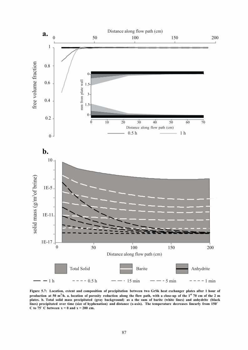
87

solid

mas

s (g/

m3 o

f brin

e)

free

vol

ume

frac

tion

mm

from

pla

te w

all

a. Distance along flow path (cm) 0 50 100 150 200

1

0.8

0.6

0 1.5

0.4

3 1.5

0.2

0

0

0 10 20 30 40 50 60 70 Distance along flow path (cm) 0.5 h 1 h

b. 10

1E-5

1E-11

1E-17 0 50 100 150 200

Distance along flow path (cm)

Total Solid Barite Anhydrite

1 h 0.5 h 15 min 5 min 1 min

Figure 5.7: Location, extent and composition of precipitation between two GrSk heat exchanger plates after 1 hour of production at 50 m3/h. a. location of porosity reduction along the flow path, with a close-up of the 1st 70 cm of the 2 m plates. b. Total solid mass precipitated (gray background) as a the sum of barite (white lines) and anhydrite (black lines) precipitated over time (size of hyphenation) and distance (x-axis). The temperature decreases linearly from 150˚ C to 75˚ C between x = 0 and x = 200 cm.

88

solid mass (g/m

3of brine) fr

ee v

olum

e fr

actio

n

5.3.3 Flow over the entire surface infrastructure

Reactive transport coupling over the entire GrSk surface infrastructure is modeled by considering the

entire length of the flow path (2600 m) with a temperature drop of 150˚ - 75˚ C at a single node in the

transport code. The system has a total volume of ~20 m3, and with a flow rate of 50 m3/h, the fluid

residence time in the system is ~25 minutes. Figure 5.8 shows the extent of free volume reduction in

the pipes and the mass of precipitation for one residence time across the entire length of the GrSk

surface infrastructure. The system’s porosity is not affected by mineral precipitation after 25 minutes

of fluid production at a rate of 50 m3/h, although ~45-65 mg/m3 of produced fluid forms during this

time frame. As is the case with the previous two models, free volume across the entire GrSk surface

infrastructure is not affected after a simulation of 1 residence time. A greater amount of precipitant

forms in one residence time of this model than the other two models, however, and it may be expected

that ~1 – 1.5 g/h of precipitant may accumulate in the system’s filters, if the model is considered as

series of individual residence times projected forward in time.

1.2

1

0.8

0.6

0.4

0.2

0

Entire surface infrastructure residence time = 25 minutes

heat exchanger

0.07 0.06 0.05

0.04 0.03 0.02 0.01 0.00

0 520 1040 1560 2080 2600 solid mass free volume fraction

Figure 5.8: Pore fraction and precipitated solid mass as a function of distance along the entire 2600 m flow length in the GrSk surface infrastructure after 1 fluid residence time (~25 minutes) at a flow rate of 50 m3/h.

The total change in porosity and precipitant mass over the 5-day duration of the simulation is show in

Figure 5.9. As expected in a 2nd order reaction, the precipitant mass increases exponentially from the

start of the model up to t = 5 days, where the total mass approaches 60 g/m3 of produced brine.

Mineral growth is accompanied by a linear decrease in the pipe’s free volume to nearly 0 after 5 days.

The location of the free volume reduction within the geothermal loop’s piping is shown in Figure

5.10a. Precipitation modeled over the 5-day span of the simulation, drives the porosity at the pipe

inflow to near 0. The precipitant mass decreases linearly from this point until ~200 m into the flow

path. After ~200, along the flow path, further precipitation in the system no longer reduces the

available flow volume in the piping. Once again, reduction in the pipe’s free volume will only occur if

89

solid mass (g/m

3of brine) fr

ee v

olum

e fr

actio

n

precipitants are not removed from the system. In reality, most precipitants will remain entrained in the

flow field and will be caught and remove by the filtration system. It may, therefore, be considered that

the greatest risk lies not in the fast reduction of free volume in the pipes, but in the cost of continually

replacing, storing, and disposing of the used filters.

1.2 60

1 50

0.8 40

0.6

0.4

0.2

0

30

20

10

0 0 20 40 60 80 100 120

hours solid mass free volume fraction

Figure 5.9: Change in pore fraction and solid mass precipitated along the entire 2600 m flow length in the GrSk surface infrastructure during 120 hours (5 days) of production at 50 m3/h

Figure 5.10b shows upwards of 10 g/m3 of brine precipitating on the hot side of the flow path, with, as

mentioned above, a sharp increase in the precipitated mass before ~ 200 m. After 200 m, the amount

of precipitant decreases linearly to about 1 g/m3 of produced brine in the vicinity of the heat

exchanger. Less precipitant forms after the heat exchanger than before it, as is also predicted by the

reactive transport model performed within the heat exchanger itself. Initially, the difference in

precipitant mass before and after the heat exchanger is only ~ 2 orders of magnitude, but after ~ 18

hours, precipitation on the cold side of the infrastructure is practically 0.

The change in the chemical composition of the precipitant over time and distance along the flow path

is depicted in Figure 5.10c. The high initial Ba:Ca ratio shows that barite precipitates first from the

brine, but after about 6 hours, anhydrite becomes the dominant precipitating phase. This same trend is

observed in the model presented in Section 5.3.1. After 6 hours, the Ba:Ca ratio continues to decrease

until the end of the 5 day simulation, at which time the barite component of the total precipitant mass

becomes vanishingly small. A similar phenomenon is observed on the cold side of the infrastructure.

Although the Ba:Ca ratio decreases with time on both sides of the heat exchanger, the Ba:Ca is always

higher on the cold side for any given time step. This observation is explained by the relative stability

of barite compared to anhydrite at low temperatures, as discussed above. Figure 5.10b also reveals

that, after a sudden, pronounced drop in the precipitated mass directly after the heat exchanger,

mineral growth is re-initiated after a distance of ~1550 m along the flow path. Essentially, the heat

90

Ba

: Ca

Rat

io

solid

mas

s (g

/m3

of b

rine)

po

rosi

ty

cm fr

om p

ipe

wal

l

exchanger resets the reaction to proceed with the system’s instantaneous chemical and kinetic values

as the input parameters in a 2nd stage of reactive transport behavior.

a. Distance along flow path (m)

0 520 1040 1560 2080 2600 1

0.8

0.6

0

2.5

1 day 3 days 5 days

0.4

0.2

0

5 2.5 0

0 50 100 150 200 250

Distance along flow path (m)

b. 1E1

heat exchanger

1E-5

1E-11

1E-17

c.

1E12

0 520 1040 1560 2080 2600

Distance along flow path (m)

heat exchanger

1E4

1E-4

1E-12

0 520 1040 1560 2080 2600 Distance along flow path (m)

0.25 h

0.5 h

1 h

6 h 18 h

24 h 48 h 72 h 96 h 120 h

Figure 5.10: Location, extent and composition of precipitation between the GrSk production pump and heat exchanger after 120 hours (5 days) of production at 50 m3/h. a. location of porosity reduction along the flow path, with a close-up of the 1st 250 m of piping. b. accumulation of solid mass as a function of time (gray scaling and hyphenation size) and distance along the production stretch (x-axis) and c. ratio of barite to anhydrite as a function of time (gray scaling and hyphenation size) and distance along the production stretch (x-axis).

91

The positive slope of the growth along the Ba:Ca ratio axis (Figure 5.10c) suggests that this 2nd round

of precipitation is dominated by barite, but the total amount of precipitant is up to 5 orders of

magnitude lower than the precipitant predicted on the hot side of the exchanger (1e-4 as opposed to

1e1 g/m3 of produced brine).

All three models presented herein show that alkali earth metal sulfate scaling is a risk primarily in the

immediate vicinity of the flow path inlet. Because these flow paths have been arbitrarily defined in

this study, it is difficult to say where exactly along the flow path precipitation will commence in the

GrSk system. The production pump is chosen as the starting point because, besides from the well

casing itself, the pump is the brine’s first contact point with the plant’s infrastructure. The results from

Chapter 3 of this study suggest that the pressure differences between the GrSk reservoir (i.e. ~ 45

MPa) and the heat exchanger (i.e. 1 MPa) do not appreciably affect the system’s equilibrium. The

effects of reservoir pressure on the precipitation kinetics remains unknown, but it is possible, if not

likely, that precipitation begins before the fluid reaches the pump (i.e. depth > 1200 m). Until the

reaction kinetics of sulfate precipitation in high pressure systems can be determined, the location of

the onset of precipitation within GrSk plant can only be determined with respect to the arbitrarily

defined starting point of the flow model.

Once precipitation is initiated, sulfate is consumed rapidly, and precipitants will most likely not

accumulate over a great lateral extent. All the models predict that precipitants will form in discrete

locations (rather than diffusely throughout the flow path). In locations where precipitants do form, the

mass will be greatest in the upstream direction and will tail off, usually linearly, in the downstream

direction. For reactive transport phenomena at 150˚ C, initial precipitation is dominated by barite, but

anhydrite precipitation becomes increasingly more prominent over time. At 75˚ C, barite is dominant

at all stages of the system’s chemical evolution, but the extent of precipitation is less at 75˚ C than at

150˚ C. This observation is in agreement with the results of the pressure and temperature effects on

barite’s logKsp made with SupCrt, presented in Chapter 2 of this study. Under isobaric conditions,

barite is slightly more soluble at 75˚ C than at 150˚ C. According to the SupCrt calculations, barite

reaches a solubility maximum between 75˚ C and 150˚ C. This calculation explains why (as shown in

Figure 5.10b) barite precipitation is strongly inhibited by the effects of the heat exchanger, but is then

re-initiated at once the brine becomes thermally stable at 75˚ C.

Finally, it must be repeated that the extent of precipitated mass predicted by these models does not

amount to a true description of scaling. Precipitants formed during geothermal brine production may

not adhere to the industrial infrastructure and may simply be captured by the plant’s filtration system.

According to the results of this study, used filters may contain as much as 60 g of solids per m3 of

filtered fluid. The average measured mass fraction of insoluble filter residue measured at GrSk (2.3.2)

is ~ 350g, but it is not known to what extent barite comprises this mass. In any case, the models do

not greatly contradict the field evidence. It is assumed that no anhydrite has been identified in the

92

field because produced fluid never reached temperatures high enough to support anhydrite stability

over barite (i.e ~135˚ C; Figure 3.4). An investigation of the conditions leading to mineral adhesion

onto the industrial framework, or factors by which precipitation can be inhibited in the produced brine,

are beyond the scope of this study.

5.4 Conclusion

Reactive transport models presented in this Chapter describe in detail the behavior of the GrSk brine as

it traverses the path from the production well pump, through the heat exchanger and back down the

injection well. Alkali-earth metal sulfates are predicted to first precipitate in the production well, and

the sulfate is generally consumed fast enough for precipitation to stop before the fluid reaches the heat

exchanger. A mass of precipitant on the order of 10s of grams per m3 of produced brine is predicted at

a production rate of 50 m3/h. If the precipitated solids are not removed from the system, free volume at

the brine’s inlet to the system (i.e. at inflow boundary) may be reduced to 0 within a week of

production time. This model, however, does not take into account the precipitant’s suspension in a

flowing fluid. At operational flow rates (i.e. ~50m3/h), it can be assumed that much of the precipitant

is transported via advection along with the moving brine mass. Entrained particles are captured by the

plant’s filtration system. The greatest immediate operating risk, therefore, to the GrSk plant, may not

be scaling in the literal sense, but in the costs of maintaining the filtration system.

93

6. Conclusion

94

6.1 Summary of Major Results Based on literature reports, initial on-site fieldwork and rudimentary geochemical modeling, it has

long been hypothesized that oversaturated minerals in the alkali-earth metal sulfate system pose a

scaling risk in the GrSk plant. The details of this scaling risk, however, have been heretofore

unknown. Operators of the GrSk plant, specifically, or any EGS plant in general, require accurate

predictive models of scaling phenomena in order to successfully manage their plants. There is also a

need in the geothermal community for a systematic methodology for designing such predictive

models. This dissertation presents the results of a comprehensive investigation of the exact nature of

the alkali-earth metal sulfate scaling risks at GrSk. Using a combination of field work, equilibrium

thermodynamic modeling, experimental geochemistry and reactive transport modeling, predictions

regarding (1) the location in the plant where minerals are most likely to precipitate, (2) the extent (by

mass) to which mineral scales may form and (3) the chemical composition of the mineral scales have

all been predicted in this study. Although it is not possible to completely verify these predictions until

the GrSk plant is able to operate more regularly, the results of this study are internally consist and in

general agreement with existing observations from the GrSk site.

Fieldwork performed during the course of this study (Chapter 2) reveal the brine produced at GrSk to

be no longer affected by the chemical influences of reservoir stimulation treatments performed from

2002-2008. Fluid chemical parameters for the GrSk brine determined in this study are essentially the

same as the initial brine’s chemistry, determined prior to any reservoir treatments. Notable exceptions

to this agreement are the sulfate, iron and lead concentrations, all of which are elevated compared to

the original data. Reasons for these differences are various, including naturally heterogeneities in the

reservoir, sampling at different locations in the geothermal loop and sampling at different

temperatures. All three of these ions (Fe, Pb, SO4) are found as major species in the filter residue

analyzed during this study. In particular, barite was found to be the most abundant, best crystallized

and largest phase found in the filter residue. This observation confirms the study’s initial hypothesis,

namely, that precipitation of alkali-earth metal sulfates presents a primary scaling risk at the GrSk

plant. Other phases, such as magnetite, laurionite, quartz, and a copper-bearing phase are also found

in the GrSk filter residue. The total mass of the insoluble portion of the filter residue ranges from 100-

500 g/m3 of brine produced.

Results from the fluid chemical analyses performed during the fieldwork section of this study are

incorporated into an equilibrium thermodynamic model of the Na-Ca-Ba-Sr-Cl-SO4-H2O components

of the GrSk brine (Chapter 3). Once again in support of this study’s initial hypothesis and field

research, barite is predicted as the predominant oversaturated phase in this system of components. In

the GrSk system, barite equilibrium is controlled by barium concentrations. Sulfate will still remain in

the system, even after barite precipitates to equilibrium. Barite is essentially insoluble, although it

95

becomes slightly soluble due to “uncommon-ion” effects in the mixed electrolyte solution. This effect

dictates that the solubility of a dissolved salt increases in the presence of a second dissolved salt with

which it contains no common ions. Such is the case with barium and sulfate in the presence of sodium

and/or calcium chloride. It is, therefore, not expected that all of the barium precipitates (as barite).

On the hot side of the GrSk heat exchanger, sulfate in excess of the barite solubility will continue to

precipitate as anhydrite, even with initial sulfate concentrations as low as 0.0005 m. Anhydrite,

however, will only precipitate on the cold side of the heat exchanger when the initial sulfate

concentration is greater than 0.001 m. The GrSk brine is anywhere from 1 g/m3 – 1 kg/m3

oversaturated with alkali-earth sulfate minerals, again depending on the initial sulfate concentration. If

only barite is considered, the oversaturation approaches 60 g/m3 at 75˚ C for sulfate concentrations

above 0.0005 m. This value is less than the total filter residue mass measured in GrSk (Chapter 2), but

the field results do not consider the mass fraction specifically of alkali-earth sulfates. In other words,

the filter residue measured in the mass-fraction experiments in Chapter 2 contained types of solids

other than sulfates. Due to insufficient material, the chemical composition of the mass fraction

experiments’ filter residue was not determined. The maximum barium concentration found in

unprocessed filter residue from inline filters is ~7%.

While equilibrium models prepared in Chapter 3 describe the general chemical tendencies of the GrSk

brine, truly predictive models require parameters describing the precipitation reactions’ kinetics.

Thus, a series of batch reaction experiments are performed (Chapter 4), aimed at deriving the kinetic

rate laws for anhydrite, barite, and celestite precipitation from a mixed electrolyte solution prepared to

be representative of sedimentary basin formation waters found worldwide. A mixed chloride salt brine

(Na-Ca-Ba-Sr-Cl-H2O) is oversaturated with a dissolved Na2SO4 aliquot, and changes in the

precipitating materials’ mass fraction, reactive surface area and chemical composition are determined

over the span of 4 hours. The precipitating phase at both 75˚ C and 150˚ C is barite. Calcium and

strontium, however, are also identified via XRF and EDX measurements, indicating that these

elements are included as accessory ions in the barite crystal lattice. Kinetic rate laws for barite and

total sulfate precipitation are determined by fitting concentration data integrated over time to a linear

function characteristic of a particular reaction order. In this method, the slope of the best-fit line is

related to the reaction rate constant k. Both barite and total sulfate precipitation proceed as 2nd order

reactions with rate constants from 0.011 – 0.045 kg of solution • millimoles of crystal-1 • seconds-1.

Spatial analyses of crystal morphology, made with the SEM, allow for estimation of the change in the

growing crystal’s reactive surface area. This parameter is the final piece required for transforming the

equilibrium model presented in Chapter 3 into a predictive risk assessment model, as discussed below.

This study concludes in Chapter 5 with the incorporation of the kinetic parameters determined in

Chapter 4 into 1-D reactive transport models of fluid flow in the GrSk surface infrastructure. Modeled

scenarios indicate that alkali-earth metal sulfate precipitation is most likely to occur in the GrSk

96

production well. The precise location of the onset of precipitation is a function of the effects of

depressurization on the ion activities and logKsp of reactive species within the brine as it ascends the

well path. All of the models show that precipitant will begin forming immediately at the start of

whatever length is arbitrarily defined as the flow path. Barite is the first forming phase in all modeled

scenarios, but anhydrite dominates the precipitant mass after a few hours of production time.

Anhydrite, however, is only predicted to form on the hot side of the heat exchanger. Barite is

predicted to form on the cold side of the heat exchanger only in the beginning of the simulations. As

the system evolves, the precipitated mass moves closer and closer to the beginning of the flow path. If

accumulated precipitants are not removed from the system, the free volume at the flow path inlet may

be reduced to 0 with a week’s production time. At this location up to 10 g/m3 of produced brine are

predicated to form. This amount trails off linearly to a distance of ~ 250 m from the inlet, where the

precipitant concentration is ~1 mg/m3 of produced brine until the location of the heat exchanger.

Precipitation on the cold side of the heat exchanger is predicted only within the first few hours of

operation. Predicted masses of precipitants, however, do not amount to a true prediction of scaling.

Such a prediction would require an investigation of adhesion mechanisms between the precipitated

crystals and the plant’s infrastructure, which is beyond the scope of this work. The total mass of

precipitants predicted by the reactive transport models neither confirms nor refutes the results from

field testing; further operations at GrSk are required to validate the models.

Taken cumulatively, the results of this study provide ample evidence that alkali-earth metal sulfate

precipitation is indeed a hazard that needs to be actively managed by plant engineers at GrSk. This

study shows that over 4 tons of sulfate precipitants may form in the GrSk system on a yearly basis.

Due to high flow rates, most of this precipitant will be entrained in the brine’s flow. Rather than

accumulating in the plant’s infrastructure, therefore, solid matter will tend to be caught and removed

by the filtration system. Thus, the real risk predicted by this study is not scaling per se, but the

consequences of having to manage the filtration system. This includes the cost of the filters, the cost

of downtime involved in changing the filters, the space require to store the used filters and the cost of

disposing of the material. Furthermore, used filters need to be monitored for radioactivity and

disposed of properly, as barite is known to incorporate environmental radium into its crystal structure

(e.g. Curti et al., 2010; Zielinksi et al., 2001; Martin and Akber, 1999; Paytan et al., 1996).

If the figure of 4 tons per year cited above seems shocking, it should be considered that this mass of

barite has a volume of ~ 0.9 m3. Spread out over a year, this appears to be a manageable volume, if a

proper system is put in place to handle it. Testing the best combinations of filters, in terms of materials

and pore sizes, for maximizing filtration throughput, can optimize the filtration system at GrSk. A

contract for regular disposal of accumulated filters must be incorporated in the plant’s budget, and

arrangements must be made for periodic measurements of the used filters’ radioactivity.

97

Planners of future EGS installations in sedimentary basins can learn from the GrSk experience by

planning ahead for the precipitation induced through production of formation fluids. The chemistry of a

geothermal system should be given careful consideration from the onset of exploration, straight

through to the design and construction of the plant. Proper consideration includes determining at what

salinities brine production becomes unsustainable, what types of precipitants are most easily managed,

what specials materials are needed to protect the plant from corrosion and what is the best way to

remove precipitated matter from the system (i.e. optimal filtration design). Such considerations

require accurate geochemical models, and accurate geochemical models are dependent on

experimentally derived data. The greatest need, therefore, amongst geochemists in the geothermal

community is reliable solubility and kinetic data upon which to construct geochemical models.

6.2 Limitations As mentioned above, the primary limitation of this study is the lack of reliable thermodynamic data for

alkali-earth metal sulfate species at the (T, p, x) conditions found in EGS systems around the world.

The most up-to-date algorithms that are widely in use are the Harvie-Møller-Weare formulations

(HMW, Harvie et al., 1984), which consider major seawater species to high concentrations, but only at

25˚ C. A more serious drawback to the HMW databases than the temperature restriction, however, is

the complete absence of barite as a mineral phase. Modeling of the GrSk brine, or any formation fluid

considered in an EGS system, is simply not possible without this data. To circumvent this problem,

this study uses the thermo_pitzer database included in the GWB software. This database contains the

necessary thermodynamic parameters for all the relevant ionic and mineral species, but is considered

outdated and is not recommended for use. A third alternative is the Quintessa® database designed for

the PHREEQc modeling program. This program also contains all of the necessary thermodynamic

data for modeling geothermal brines, but has not undergone any peer review. The thermo_pitzer

database was chosen for ease of use with the advanced features of the GWB, such as the kinetic and

reactive transport modeling functions. Dependable geochemical models, including those based on

experimentally derived kinetic data, require accurate descriptions of thermodynamic equilibrium and

proper determination of activity coefficients at the temperatures and pressures under consideration.

These fundamental parameters for EGS systems in sedimentary basins remain undetermined. Despite

the detailed kinetic parameters incorporated into this study’s reactive transport models, therefore, the

models’ predictions still must be taken tentatively.

This study is also limited by ongoing development of the experimental infrastructure, combined with

the challenges involved in chemical analyses of highly saline solutions. During the design and testing

phase of the experimental apparatus presented in Chapter 4, many hundreds of experimental fluid

98

samples were analyzed with optical emissions spectroscopy (for cation ions) and ion chromatography

(anions), with mixed results. Problem arose with trying to detect trace element concentrations (i.e.

barium, strontium, sulfate) in the thick Na-Ca-Cl background solutions. Diluting the solution

prevented the salinity from damaging the IC columns, but it did not change the fundamental ratio of

major to trace elements. Attempts were made to only measure cations in an undiluted solution, but in

addition to assisting with the analyses, the dilution also prevented additional post-experimental

precipitation from occurring. Thus, attempts to measure chemical changes in the fluid were

abandoned altogether in favor of the solid phase analytical methods presented in Chapters 2 and 4 of

the work. Handling of the solid phases between the experiment and the analyses was simpler and less

prone to contamination than handling of the fluid phase. Furthermore, the solid phase has a longer

shelf life than the liquid phase, if analyses cannot be immediately performed. The only major

drawback with the solid phase analytics is that the autoclaves were often too small to generate enough

filter residues for the XRF. Futures studies of this nature would benefit greatly from a larger (e.g.

1000 ml) autoclave. For ease of mass balance calculations when working with the filter residue, it is

important to prepare all experimental solutions in molal (rather than molar) concentrations.

Finally, the reactive transport models presented in this study are limited by a lack of field confirmation

of their accuracy. The model predicts the prevalence of anhydrite after 6 hours of production, but, to

date, no anhydrite has been found. It is rare, however, that the plant has been able to operate for 6

hours at time, and when it has, the flow rate has been much lower than 50 m3/h. Additionally, the

plant has never produced fluid over 110˚ C at the surface. Once the plant stops producing and the

fluid cools down, the modeled simulations need be restarted from time = 0. The discrepancy between

the models’ predictions of anhydrite scaling and the lack of anhydrite observed in the GrSk filter

residue, therefore, may not be due to inaccuracies in the model. Rather, it is possible that the plant has

not yet reached the degree of functionality simulated by the model. In either case, the model cannot be

fully validated until regular operations, i.e. production of hot brine at flow rates conducive to

electricity production, at the GrSk site can be established.

6.3 Broader impacts This dissertation is quite narrowly focused on the GrSk system as a case study for EGS development

in sedimentary basins worldwide. An argument can be made showing the GrSk brine to be

representative of many formation fluids found in sedimentary basins around the world, and the results

from this study may be extrapolated to other systems in a fairly straightforward manner. In particular,

the kinetic experiments presented in Chapter 4 employed experimental solutions meant to be more

indicative of the general case of geothermal brines, rather than just a replica of the GrSk fluid. The

99

rate laws derived in Chapter 4 can, therefore, in the absence of other experimental data, be used to

model alkali-earth metal sulfate precipitation in brines of similar ionic strength with a fair degree of

reliability. The form in which precipitants accumulate in the production line, as modeled in Chapter 5

of this study, will certainly be of interest to plant operators in a variety of settings.

On the other hand, an argument can be made showing the GrSk fluid to be quite extra-ordinary

concerning both its overall salinity and its complex elemental composition. In this case, the broader

impacts of this study lie not with the specific results presented herein, but the methodologies employed

to the assess the scaling risk in the GrSk system. This dissertation details a step-by-step method by

which scaling hazards in any geothermal system, be it conventional or EGS, in a sedimentary basin or

artificially fractured granite, can be quantitatively assessed. Furthermore, the experimental

methodology presented herein can be used to investigate mineral solubilities and precipitation kinetics

in a variety of geochemical systems over a wide range of temperature and pressure conditions. A

particularly unique feature of the experimental apparatus developed in the course of this study is its

extreme corrosion resistance. This apparatus continues to be employed in research with corrosive

geothermal fluids, beyond the immediate scope of this study.

6.4 Suggestions for further research The research presented in this study represents the results of the start-up project for the

hydrochemistry laboratory at the International Center for Geothermal Research, GFZ-Potsdam; there

are practically unlimited directions in which this research can expand. The experimental methodology

developed in this study is currently being used to test the efficacy of solutions designed to inhibit

mineral precipitation in a variety of geothermal brines found in Germany. Studies similar to the one

presented herein can be performed for other expected scaling forming mineral in the GrSk system. Of

particular concern are iron, copper, and lead bearing phases, which have all been identified in the GrSk

filter residue. Silicates, especially zeolites, may also pose a scaling risk in the vicinity of the GrSk

injection well. From a methodological point of view, the performance of these experiments would

benefit from a larger autoclave. A research and design investment in a reactor unit custom designed

and constructed at the GFZ would allow the incorporation of many features not available on the open

market. Finally, as mentioned above, the most important area for further research of scaling

phenomena in geothermal brines is in the updating of existing Pitzer parameters for a variety of

species, but most importantly Ba, Fe, Pb, Cu, Si and Al.

100

References Akaku K., 1990: Geochemical study on mineral precipitation from geothermal waters at the Fushime

field, Kyushu, Japan, Geothermics, 19, pp 455-467 Allison J.D., Brown D.S. and Novo-Gradac K.J., 1991: MINTEQA2/PRODEFA2, a geochemical

assessment model for environmental systems: Version 3.0 user’s manual, Environmental Research Laboratory, Office of Research and Development, U.S. Environmental Protection Agency, Georgia, USA

Archibald D.D., Gaber B.P., Hopwood J.D., Mann S. and Boland T., 1996: Atomic force microscopy

of synthetic barite microcrystals, Journal of Crystal Growth, 172, pp 231-248 Atkinson R.J., 1977: Crystal nucleation and growth in hydrolyzing iron(III) chloride solutions, Clays

and Clay Minerals, 25, pp 49-56 Azaroual M., Fouillac C. and Matray J.M., 1997: Solubility of silica polymorphs in electrolyte

solutions: I. Activity coefficient of aqueous silica from 25˚ to 250˚ C, Pitzer’s parameterization, Chemical Geology, 140, pp 155-165

Baccar M.B., Fritz B. and Brevart O., 1993: Geochemical modeling of late diagenetic processesin the

Brent Sandstone, Alwyn South area (East Shetland Basin, North Sea) 1. Estimation of the circulated fluids composition, Chemical Geology, 109, pp 135-147

Ball J.W. and Nordstrom D.K., 1991: User’s manual for WATEQ4F, with revised thermodynamic

database and test cases for calculating speciation of major, trace, and redox elements in natural waters, Open-file Report, United States Geological Survey, California, USA

Barge D., Al-Yami F., Uphold D., Zahedi A. and Deemer A., 2009: Steamflood piloting the Wafra

Field Eocene reservoir in the partitioned neutral zone, between Saudi Arabia and Kuwait, Society of Petroleum Engineers Middle East Oil and Gas Show and Conference, Conference Paper, 120205-MS, Bahrain, Bahrain

Bayer U., Scheck M. and Koehler M., 1997: Modeling of the 3-D thermal field in the northeast

German basin, Geologische Rundschau, 86, pp 241-251 Bayer U., Scheck M., Rabbel W., Krawczyk C.M., Götze H.-J., Stiller M., Beilecke Th., Marotta A.-

M., Barrio-Alvers L. and Kuder J., 1999: An integrated study of the NE German Basin, Tectonophysics, 314, pp 285-307

Bazin B. and Brosse E., 1997: Chemistry of oil-field brines in relation to diagenesis of reservoirs 1.

Use of mineral stability fields to reconstruct in situ water composition. Example of the Mahakam basin, Marine and Petroleum Geology, 14, pp 481-495

Benek R., Kramer W., McCann T., Scheck M., Negendank J.F.W., Korich D., Huebscher H.-D. and

Bayer U., 1996: Permo-Carboniferous magmatism of the Northeast German Basin, Tectonophysics, 266, pp 379-404

Bethke, 2008: Geochemical and biogeochemical reaction modeling, Cambridge University Press, New

York

101

Bethke C.M., 1992: The question of uniqueness in geochemical modeling, Geochimica et Cosmochimica Acta, 56, pp 4315-4320

Bertani R., 2012: Geothermal power generation in the world 2005-2010 update report, Geothermics,

41, pp 1-29 BinMerdhah A.B. and Yassin A.A.M, 2007: Barium sulfate scale formation in oil reservoir during

water injection at high-barium formation water, Journal of Applied Sciences, 7, pp 2393-2403 BinMerdhah A.B., Yassin A.A.M., and Muherei M.A., 2009: Laboratory and prediction of barium

sulfate scaling at high-barium formation water, Journal of Petroleum Science and Engineering, 70, pp 79-88

Bird G., Boon J. and Stone T., 1986: Silica transport during steam injection into oil sands, dissolution

and precipitation kinetics of quartz: New results and review of existing data, Chemical Geology, 54, pp 69-80

Blackwell D. D., Negraru P.T., Richards M.C., 2007: Assessment of the enhanced geothermal

resource base of the United States, Natural Resource Research, 15, 4 Block J. and Waters O.B., 1968: The CaSO4-Na2SO4-NaCl-H2O at 25˚ C to 100˚ C, Journal of

Chemical and Engineering Data, 13, pp 336-344 Blount, C.W., 1977: Barite solubilities and thermodynamic quantities up to 300˚ C and 1400 bar,

American Mineralogist, 62, pp 942-957 Blount C.W. and Dickson F.W., 1969: The solubility of anhydrite (CaSO4) in NaCl-H2O from 100 to

450˚ C and 1 to 1000 bars, Geochimica et Cosmochimica Acta, 33, pp 227-245 Bock, E., 1961: On the solubility of anhydrous calcium sulphate and gypsum in concentrated of

solutions of sodium chloride at 25˚ C, 30 ˚ C, 40˚ C, and 50˚ C, Canadian Journal of Chemisty, 39, pp 1746-1751

Bosbach D., Hall C. and Putnis A., 1998: Mineral precipitation and dissolution in aqueous solution: in-

situ microscopic observations on barite (001) with atomic force microscopy, Chemical Geology, 15, pp 143-160

Breitkreuz C. and Kennedy A., 1999: Magmatic flare-up at the Carboniferous/Permian boundary in the

NE German Basin revealed by SHRIMP zircon ages, Tectonophysics, 302, pp 307-326 Brink H.J., Dürschner H. and Trappe H., 1991: Some aspects of the late and post-Variscan

development of the Northwestern German Basin, Tectonophysics, 207, pp 65-95 Cataldi R., S.F. Hodgson, J.W. Lund, 1999: Stories from a Heated Earth – Our Geothermal Heritage.

Geothermal Resources Council, Davis, California, 580 pp Cermak V., 1993: Lithospheric thermal regimes in Europe, Physics of the Earth and Planetary

Interiors, 79, pp 179-193 Collins I.R., Stalker R. and Graham G.M., 2004: Sulphate removal for barium sulfate scale mitigation:

a deepwater subsea production system, Society of Petroleum Engineers International Symposium on Oilfield Scale, Conference Paper, 87465-MS, Aberdeen, UK

Collins I.R., 2005: Predicting the location of barium sulfate scale formation in production systems,

102

Society of Petroleum Engineers International Symposium on Oilfield Scale, Conference Paper, 94366-MS, Aberdeen, UK

Caroll S., Mroczek E., Alai M. and Ebert M., 1998: Amorphous silica precipitation (60 to 120˚ C):

comparison of laboratory and field rates, Geochimica et Cosmochimica Acta,62, pp 1379-1396 Christy A.G. and Putnis A., 1993: The kinetics of barite dissolution and precipitation in water and

sodium chloride brines at 44˚ - 85˚ C, Geochimica et Cosmochimica Acta, 57, pp 2161-2168 Cody R.D. and Hull A.B., 1980: Experimental growth of primary anhydrite at low temperatures and

water salinities, Geology, 8, pp 505-509 Coward M.P., 1995: Structural and tectonic setting of the Permo-Triassic basins of northwest Europe,

in: Boldy S..A.R. (ed), 1995: Permian and Triassic Rifting in Northwest Europe, Geological Society Special Publication, 91, pp 7-39

Criaud A. and Fouillac C., 1989: Sulfide scaling in low enthalpy geothermal environments: A survey,

Geothermics, 18, pp 73-81 Curti E., Fujiwara K., Iijima K., Tits J., Cuesta C., Kitamura A., Glaus M.A. and Müller W., 2010:

Radium uptake during barite recrystallization at 23 +/- 2˚ C as a function of solution composition: An experimental 133Ba and 226Ra tracer study

D’amore F., Giusti D. and Abdallah A., 1997: Geochemistry of the high-salinity geothermal field of

Asal, Republic of Djibouti, Africa, Geothermics, 27, pp 197-210 Davis R.A. and McElhiney J.E., 2002: The advancement of sulfate removal from seawater in offshore

waterflood operations, NACE International Corrosion 2002, Conference Paper, 02314, Colorado, USA

Dadlez R., Narkiewicz M., Stephenson R.A., Visser M.T.M. and van Wees J.-D., 1995: Tectonic

evolution of the Mid-Polish Trough: modeling implications and significance for central European geology, Tectonophysics, 252, pp 179-195

Debye P. and Hückel E., 1923: Zur Theorie der Elektrolyte, Physikalische Zeitschrift, 9, pp 185-206

Devidal J., Schott J. and Dandurand J., 1997: An experimental study of kaolinite dissolution and

precipitation kinetics as a function of chemical affinity and solution composition at 150˚ C, 40 bars, and pH 2, 6.8 and 7.8, Geochimica et Cosmochimica Acta, 1, pp 5165-518

Dickson F.W., Blount C.W. and Tunell G., 1963: Use of hydrothermal solution equipment to

determine the solubility of anhydrite in water from 100˚ C to 275˚ C and from 1 bar to 1000 bars of pressure, The American Journal of Science, 261, pp 61-78

DiPippo R., 2004: Second Law assessment of binary plants generating power from low-temperature

geothermal fluids. Geothermics, 33, pp 565–586. Dixon M.H. and Fanelli M., 2003. Geothermal background. In: Dickson, M.H., Fanelli, M. (Eds.),

Geothermal Energy: Utilization and Technology, UNESCO Renewable Energy Series. Earthscan Publications Ltd., London, UK, pp. 1–28

Drever J.I. (ed.), 2002: The geochemistry of natural waters: Surface and groundwater environments,

Prentice Hall, New Jersey, USA

103

Dreybrodt W., Eisenlohr L., Madry B. and Ringer S., 1997: Precipitation kinetics of calcite in the system CaCO3 – H2O – CO2: The conversion to CO2 by the slow process H+ -- HCO3

- CO2 + H2O as a rate limiting step, Geochimica et Cosmochimica Acta, 18, 3897-3904

El-Hattab M.I., 1985: Scale deposition in surface and subsurface production equipment in the Gulf of

Suez, Journal of Petroleum Technology, 37, pp 1640-1652 Erdlac Jr. R.J., Armour L., Lee R., Snyder S., Sorenson M., Matteucci M., Horton J., 2007: Ongoing

resource assessment of geothermal energy from sedimentary basins in Texas, Proceedings, Thirty-second Workshop on Geothermal Reservoir Engineering, Stanford University, USA

Eugster H.P. and Jones B. F., 1979: Behavoir of major solutes during closed-basin brine evolution,

American Journal of Science, 279, pp 609-631 Falta R.W., Pruess K., Finsterle S. and Battistelli A., 1995: T2VOC user’s guide, Lawrence Berkeley

National Laboratories, U.S. Department of Energy, California, USA Fan C., Kan A. and Tomson M.B., 2009: Barite nucleation and inhibition at 0-200˚ C, with and

without hydrate inhibitors, Society of Petroleum Engineers International Symposium on Oilfield Chemistry, Conference Paper, 121559-MS, Texas, USA

Fontes J.Ch. and Matray J.M., 1993: Geochemistry and origin of formation brines from the Paris

basin, France, Chemical Geology, 109, pp 177-200 Förster, A., 2001: Analysis of borehole temperature data in the Northeast German Basin: continuous

logs versus bottom-hole temperatures, Petroleum Geoscience, 7, pp 241-254 Franco A. and Villani M., 2009: Optimal design of binary cycle power plants for water-dominated,

medium-temperature geothermal fields, Geothermics, 38, pp 379-391 Frape S.K., Blyth A., Blomkvist R., McNutt R.H. and Gascoyne M., 2004: Deep fluids in the

continents: II. Crystalline rocks. in J.I. Drever, H.D. Holland, K.K. Turekian (eds.), Treatise on Geochemistry, vol. 5, Surface and Groundwater, Weathering, and Soils, pp 541-58

Frick S., Kaltscmitt M., Schöder G., 2010: Life cycle assessment of geothermal binary power plants

using low-temperature reservoirs, Energy, 35, pp 2281-2294 Frick S., Regenspurg S., Kranz S., Milsch H., Saadat A., Francke H., Brandt W. and Huenges E.,

(2011): Geochemical and process engineering challenges for geothermal power generation. Chemie Ingenieur Technik, 83, pp 2093 2104

Fritz B. and Noguera C., 2009: Mineral precipitation kinetics, Reviews in Mineralogy and Geochemistry, 70, pp 371-410

Fulford R.S., 1968: Effects of brine concentration and pressure drop on gypsum scaling in oil wells,

Journal of Petroleum Technology, 20, pp 559-564 Ganor J., Huston T.J. and Walter L.M., 2004: Quartz precipitation kinetics at 180˚ C in NaCl

solutions—implications for the usability of the principle of detailed balancing, Geochimica et Cosmochimica Acta, 69, pp 2043-2056

Gardner G.L. and Nancollas G.H., 1983: Crystal growth in aqueous solution at elevated temperatures.

Barium sulfate growth kinetics, Journal of Physical Chemistry, 87, pp 4699-4703

104

Gawell K., Reed M., Wright P.M., 1999: Preliminary report: Geothermal energy, the potential for clean power from the Earth, Geothermal Energy Association, Washington D.C., USA

Genter A., Guillou-Frottier L., Feybesse J., Nicol N., Dezayes C., Schwartz S., 2003: Typology of hot

fractured rock resources in Europe, Geothermics, 32, pp 701-710 Giese L., Seibt A., Wiersberg T., Zimmer M., Erzinger J., Niedermann S. and Pekdeger A., 2002:

Geochemie der Formationsfluide (Geochemistry of the Formationfluids), in: Huenges E. (ed.), 2001: In-situ Geothermielabor Groß Schönebeck: Bohrarbeiten, Bohrlochmessungen, Hydraulik, Formationsfluide, Tonminerale (In-Situ Geothermal Laboratory Groß Schönebeck: Drilling, logging, hydraulic test, formation fluids and clay minerals) Scientific Technical Report STR02/41, Helmholtz-Zentrum Potsdam- Deutsches GeoForschungsZentrum, Potsdam, Germany, pp 145-170

Gill J.S. and Nancollas G.H., 1979: Kinetics of growth of calcium sulfate crystals at heated metal

surfaces, Journal of Crystal Growth, 48, pp 34-40 Gislason S.R., Heaney P.J., Oelkers E. H. and Schott J., 1997: Kinetic and thermodyanimc properties

of moganite, a novel silica polymorph, Geochimica et Cosmochimica Acta, 61, pp 1193-1204 Glater J. and Fung K., 1969: Calcium sulfate hemihydrate scaling thresholds in natural waters from

100˚ to 150˚ C, Environmental Science and Technology, 3, pp 580-584 Glennie K.W., 1995: Permian and Triassic rifting in northwest Europe, in: Boldy S..A.R. (ed), 1995:

Permian and Triassic Rifting in Northwest Europe, Geological Society Special Publication, 91, pp 1-5

Gluyas J., Jolley L. and Primmer T., 1993: Element mobility during diagenesis: sulphate cemetation of

Rotliegend sandstones, Southern North Sea, Marine and Petroleum Geology, 14, pp 1004- 1011 Gottschalk M., 2007: Equations of state for complex fluids, Reviews in Mineralogy and Geochemistry,

65, pp 49-97 Greenberg J.P. and Moller N., 1989: The prediction of mineral solubilities in natural waters: A

chemical equilibrium model for the Na-K-Ca-Cl-SO4-H2O system to high concentration from 0 to 250˚ C, Geochimica et Cosmochimica Acta, 53, pp 2503-2518

Grundl T. and Delwiche J., 1993: Kinetics of ferric oxyhydroxide precipitation, Journal of

Contaminant Hydrology, 14, pp 71-97 Gunnarsson I., Arnorsson S. and Jakobsson S., 2005: Precipitation of poorly crystalline antigorite

under hydrothermal conditions, Geochimica et Cosmochimica Acta, 69, pp 2813-2828 Gunnarsson I. and Arnorsson S., 2005: Impact of silica scaling on the efficiency of heat extraction

from high-temperature geothermal fluids, Geothermics, 34, pp 320-329 Hanor J.S., 1993: Physical and chemical controls on the composition of waters in sedimentary basins,

Marine and Petroleum Geology, 11, pp 31-45 Hanor J.S., 1994: Origin of saline fluids in sedimentary basins, in J. Parnell (ed.), 1994: Geofluids:

origin, migration and evolution of fluids in sedimentary basins, Geological Society Special Publication No. 78, pp 151-174

Hartmann A., Pechnic R., Clauser C., 2008: Petrophysical analysis of regional-scale thermal properties

105

for improved simulations of geothermal installations and basin-scale heat and fluid flow, Internation Journal of Earth Sciences (Geologische Rundschau), 97, pp 421-433

Harvie C.H., Greenberg J.P. and Weare J.H., 1987: A chemical equilibrium algorithm for highly non-

ideal multiphase systems: Free energy minimization*, Geochimica et Cosmochimica Acta, 51, pp 1045-1057

Harvie C.H., Moller N. and Weare J.H., 1984: The prediction of mineral solubilities in natural waters:

the Na-K-Mg-Ca-H-Cl-SO4-OH-HCO3-CO3-CO2-H2O system to high ionic strength at 25˚ C, Geochimica et Cosmochimica Acta, 48, pp 723-751

Harvie C.H., Eugster H.P. and Weare J.H., 1982: Mineral equilibria in the six-component seawater

system, Na-K-Mg-Ca-SO4-Cl-H2O at 25˚ C. II: Compositions of the saturated solutions, Geochimica et Cosmochimica Acta, 46, pp 1603-1618

Harvie C.E and Weare J.H., 1980: The prediction of mineral solubilities in natural waters: the Na-K-

Mg-Ca-Cl-SO4-H2O system from zero to high concentration at 25˚ C, Geochimica et Cosmochimica Acta, 44, pp 981-997

Hasson D. and Zahavi J., 1970: Mechanism of calcium sulfate scale deposition on heat-transfer

surfaces, I & EC Fundamentals, 9, pp 1-10 He S., Oddo J.E. and Tomson M.B., 1994: The inhibition of gypsum and barite nucleation in NaCl

brines at temperatures from 25-90˚C, Applied Geochemistry, 9, pp 561-567 Heberle F. and Brüggemann D., 2010: Exergy based fluid selection for a geothermal organic rankine

cycle for combined heat and power generation, Applied Thermal Engineering, 30, pp 1326-1332 Helgeson H.C., 1968: Geologic and thermodynamic characteristics of the Salton Sea geothermal

system, American Journal of Science, 266, pp 129-166 Henninges J., Zimmerman G., Büttner G., Schrötter J., Erbas K. and Huenges E., 2005: Wireline

distributed temperature measurements and permanent installations behind casing, Proceedings, World Geothermal Congress 2005, Antalya, Turkey

Hettiarachchi H.D.M., Golubovic M., Worek W.M., Ikegame Y., 2007: Optimum design criteria for an

organic rankine cycle using low-temperature geothermal heat sources, Energy, 32, pp 1698-1706 Holl H., Hurter S., Saadat A., S. Köhler M., Wolfgramm, Zimmermann G., Trautwein U., Winter H.,

Legarth B. and Huenges E., 2003: First hand experience in a second hand borehole: Hydraulic experiments and scaling in the geothermal well Groß Schönebeck after reopening, Proceedings, Internation Geothermal Conference, Reykjavik, Iceland

Hsu P.H., 2006: Nucleation, polymerization and precipitation of FeOOH, Journal of Soil Science, 23,

pp 409-419 Huenges E. (ed.), 2002: In-situ Geothermielabor Groß Schönebeck: Bohrarbeiten,

Bohrlochmessungen, Hydraulik, Formationsfluide, Tonminerale (In-Situ Geothermal Laboratory Groß Schönebeck: Drilling, logging, hydraulic test, formation fluids and clay minerals) Scientific Technical Report STR02/41, Helmholtz-Zentrum Potsdam- Deutsches GeoForschungsZentrum, Potsdam, Germany

Huenges E., Holl H., Legarth B., Zimmerman G. and Saadat A., 2004: The stimulation of a

106

sedimentary geothermal reservoir in the northeast German basin: case study Groß Schönebeck, Proceedings, Twenty ninth Workshop on Geothermal Reservoir Engineering, Stanford University, USA

Huenges E., Moeck I. and Geothermal Project Group, 2007: Directional drilling and stimulation of a

deep sedimentary geothermal reservoir. Scientific Drilling, 5, pp 47-49 Huenges E., 2010: Tiefe Geothermie in Deutschland - eine Übersicht, Fachmagazin für Brunnen- und

Leitungsbau, Sonderheft, Tiefe Geothermie, p 6-13 Hurter S., 2002: The In-Situ Geothermal Laboratory Groß Schönebeck: a brief history, in: Huenges E.

(ed.), 2001: In-situ Geothermielabor Groß Schönebeck: Bohrarbeiten, Bohrlochmessungen, Hydraulik, Formationsfluide, Tonminerale (In-Situ Geothermal Laboratory Groß Schönebeck: Drilling, logging, hydraulic test, formation fluids and clay minerals), Scientific Technical Report STR02/41, Helmholtz-Zentrum Potsdam- Deutsches GeoForschungsZentrum, Potsdam, Germany, pp 7-20

Inches C.E., El Doueiri K. and Sorbie K.S., 2006: Green inhibitors: Mechanisms in the control of

barium sulfate scale, NACE International Corrosion 2006, Conference Paper, 06485, California, USA

Jacobson M. Z., 2009: Review of solutions to global warming, air pollution, and energy security.

Energy and Environmental Science. 2, pp.148-173 Jessop A.M. and Majorowicz J.A., 1994: Fluid flow and heat transfer in sedimentary basins, in

Parnell, J. (ed.), 1994: Geofluids: origin, migration and evolution of fluids in sedimentary basins, Geological Society Special Publication #78, pp 43-54

Johnson J.W., Oelkers E.H. and Helgeson H.C., 1992: SupCrt92: A software package for calculating

the standard molal thermodynamic properties of minerals, gases, aqueous species, and reactions from 1 to 5000 bar and 0 to 1000˚ C, Computers and Geosciences, 18, pp 899-947

Jones P.H., 1970: Geothermal resources of the northern Gulf of Mexico basin, U.N. Symposium on the

Development and Utilization of Geothermal Resources, Pisa, Italy Kaiser A., Reicherter C., Hübscher C. and Gajewski D., 2005: Variation of the present-day stress field

within the Northern German Basin—insights from thin shell FE modeling based on residual GPS velocities, Tectonophysics, 397, pp 55-72

Kan A.T., Fu G., Watson A. and Tomson M.B., 2002: Effect of hydrate inhibitors on oilfield scale

formation and inhibition, Society of Petroleum Engineers International Symposium on Oilfield Scale, Conference Paper, 74657-MS, Aberdeen, UK

Kharaka Y.K., Hull R.W. and Carothers W.W., 1985: Water rock interactions in sedimentary basins, in

D.L. Gautiers, Y.K. Kharaka and R.C. Surdam (eds.), Relationship of Organic Matter and Mineral Diagenesis: Society of Economic Patrolytes, American Journal of Scinence, 288, pp 19-9

Kharaka Y.K., Gunter W.D., Aggarwal P.K., Perkins E.H. and DeBraal J.D., 1988: SOLMINEQ.88: A

computer program for geochemical modeling of water-rock interactions, Water-resources Investigations Report 88-4227, United States Geological Survey, California, USA

Kharaka Y.K. and Hanor J.S., 2004: Deep fluids in the continents: I: Sedimentary rocks, in J.I. Drever,

H.D. Holland, K.K. Turekian (eds.), Treatise on Geochemistry, vol. 5, Surface and Groundwater,

107

Weathering, and Soils, pp 499-540 Kowacz M., Putnis C.V. and Putnis A., 2007: The effect of cation:anion ration in solution on the

mechanism of barite growth at constant supersaturation: Role of the desolvation process on the growth kinetics, Geochimica et Cosmochimica Acta, 71, pp 5168-5179

Kranz S., Saadat A., Frick S., Francke H. and Thorade M., 2010: Forschungskraftwerk Groß

Schönebeck, anlagenkonzept und forschungsziele, Der Geothermiekongress 2010, Karlsruhe, Germany

Krumgalz B., 2001: Application of the Pitzer ion interaction model to natural hypersaline brines,

Journal of Molecular Liquids, 91, pp 3-19 Kuhn T., Herzig P.M., Hannington M.D., Garbe-Schönberg D. and Stoffers P., 2003: Origins of fluids

and anhydrite precipitation in the sediment-hosted Grimsey hydrothermal field north of Iceland, Chemical Geology, 202, pp 5-21

Kühn M., Frosch G., Kölling M., Kellner T., Althaus E. and Schulz H.D., 1997: Experimentelle

Untersuchungen zur Barytübersättigung einer Thermalsole, Grundwasser—Zeitschrift der Fachsektion Hydrogeologie, 3/97, pp 111-117

Kühn M., Niewöhner C., Isenbeck-Schröter M. and Schulz H.D., 2007: Determination of major and

minor constituents in anoxic thermal brines of deep sandstone aquifers in northern Germany, Water Research, 32, pp 265-274

Legarth B., Huenges E. and Zimmermann G., 2005: Hydraulic fracturing in a sedimentary geothermal

reservoir: Results and implications, International Journal of Rock Mechanics & Mining Sciences, 42, pp 1028-1041

Lenz G. and Hoffmann F., 2002: Planung und Durchführung der Aufwältigungs-, Bohr- und

Testarbeiten (Planning and Realization of Drilling and Testing Operations), in: Huenges E. (ed.), 2001: In-situ Geothermielabor Groß Schönebeck: Bohrarbeiten, Bohrlochmessungen, Hydraulik, Formationsfluide, Tonminerale (In-Situ Geothermal Laboratory Groß Schönebeck: Drilling, logging, hydraulic test, formation fluids and clay minerals) Scientific Technical Report STR02/41, Helmholtz-Zentrum Potsdam- Deutsches GeoForschungsZentrum, Potsdam, Germany, pp 21-42

Littke R., Bayer U. and Gejewski D., 2005: Dynamics of sedimentary basins: the example of the

Central European Basin system, International Journal of Earth Sciences (Geologisches Rundschau), 94, pp 779-781

Lu C.H. and Fabuss B.M., 1968: Calcium sulfate scaling in saline water distribution, I & EC Process

Design and Development, 7, pp 206-212 Lund J.W., Freeston D. H., Boyd T.L., 2010: Direct utilization of geothermal energy 2010 worldwide

review, Geothermics, 40, pp 159-180 Lueders V., Plessen B., Romer R.L., Weise S.M., Banks D.A., Hoth P., Dulksi P. and Schettler G.,

2010: Chemistry and isotopic composition of Rotliegend and Upper Carboniferous formation waters from the North German Basin, Chemical Geology, 276, pp 198-208

Lüders V., Reutel C., Hoth P., Banks D.A., Mingram B. and Pettke T., 2005: Fluid and gas migration in

the North German Basin: fluid inclusion and stable isotope constraints, International Journal of Earth Sciences (Geologisches Rundschau), 94, pp 990-1009

108

Mackay E.J. and Graham G.M, 2003: The use of flow models in assessing the risk of scale damage, Society of Petroleum Engineers International Symposium on Oilfield Chemistry, Conference Paper, 80252-MS, Texas, USA

Mackay E.J., 2002: Modeling of in-situ scale deposition: The impact of reservoir and well geometries

and kinetic reaction rates, Society of Petroleum Engineers International Symposium on Oilfield Scale, Conference Paper, 74683-MS, Aberdeen, UK

Manning D.A.C, Younger P.L., Smith F.W., Jones J.M., Dutton D.J., Diskin S., 2007: A deep

exploration well at Eastgate, Weardale, UK: a novel exploration concept for low-enthalpy resources, Journal of the Geological Society of London, 164, pp 371-382

Majorowicz J.A. and Jessop A.M., 1981: Regional heat flow patterns in the western Canadian

sedimentary basin, Tectonophysics, 74, pp 209-238 Marshall, W.L. and Slusher, R., 1966: Thermodynamics of calcium sulfate dehydrate in aqueous

sodium chloride solutions, 0-110˚, Journal of Physical Chemistry, 70, pp 4015-4027 Martin J.T. and Lowell R.P, 2000: Precipitation of quartz during high temperature, fracture-controlled

hydrothermal upflow at ocean ridges: equilibrium versus linear kinetics, Journal of Geophysical Research, 105, pp 869-882

Martin P. and Akber R.A., 1999: Radium isotopes as indicators of adsorption-desorption interactions

and barite formation in groundwater, Journal of Environmental Radioactivity, 46, pp 271-286 Maystrenko Y.P., Bayer U and Scheck-Wenderoth M., 2012: Salt as a 3D element in structural

modeling—Example from the Central European Basin System, Tectonophysics, (available online: 2012)

Menning M., Alekseev A.S., Chuvashov B.I., Davydov V.I., Devuyst F.-X., Forke H.C., Grunt T.A.,

Hance L., Heckel P.H., Izokh N.G., Jin Y.-G., Jones P.J., Kotlyar G.V., Kozur H.W., Nemyrovska T.I., Schneider J.W., Wang X.-D., Weddige K., Weyer D. and Work D.M., 2006: Global times scale and regional stratigraphic reference scales of Central and West Europe, East Europe, Tehys, South China, and North America as used in the Devonian—Carboniferous—Permian correlation chart 2003 (DCP 2003), Palaeogeography, Palaeoclimatology, Palaeoecology, 240, pp 318-372

Meer S.D., Spiers C.J. and Peach C.J., 2000: Kinetics of precipitation of gypsum and implications for

pressure-solution creep, Journal of the Geological Society of London, 157, pp 269-281 Milsch H., Regenspurg S., Brandt W., Giese R., Poser M., Kratz A., Kranz S., Schmidt K. and Saadat

A., 2010: FluMo- A mobile fluid-chemical monitoring unit for geothermal plants, Der Geothermiekongress 2010, Karlsruhe, Germany

Minissale A., Borrini D., Montegrossi G., Orlando A., Tassi F., Vaselli O., Huertas A.D., Yang J.,

Cheng W., Tedesco D. and Poreda R., 2008: The Tianjin geothermal field (north-eastern China): Water chemistry and possible reservoir permeability reduction phenomena, Geothermics, 37, pp 400-428

Millero F.J., 2009: Thermodynamic and kinetic properties of natural brines, Aquatic Geochemistry, 15,

pp 7-41 Millero F.J., DiTrolio B., Suarez F.A. and Lando G., 2009: Spectroscopic measurements of the pH in

NaCl brines, Geochimica et Cosmochimica Acta, 73, pp 3109-3114

109

MIT (Massachusetts Institute of Technology), 2006: The Future of Geothermal Energy: Impact of Enhanced Geothermal Systems (EGS) on the United States in the 21st Century, prepared under contract for the U.S. Government under D.O.E. Contract DE-AC07-05ID14517

Moeck I., Schandelmeier H. and Holl H.G., 2009: The stress regime in a Rotliegend reservoir of the

Northeast German Basin, International Journal of Earth Sciences (Geologisches Rundschau), 98, pp 1643-1654

Moghadasi J., Jamialahmadi M., Müller-Steinhagen H., Sharif A., Ghalambor A., Izadpanah M.R. and

Motaie E., 2003: Scale formation in Iranian oil reservoir and production equipment during water injection, Society of Petroleum Engineers International Symposium on Oilfield Scale, Conference Paper, 80406-MS, Aberdeen, UK

Moller N. and Weare J.H., 1999: Models of geothermal brine chemistry, U.S. Department of Energy

Final Report DE-FG07-93ID13247, California, USA Monnin C., 1998: A thermodynamic model for the solubility of barite and celestite in electrolyte

solutions and seawater to 200˚ C and to 1 kbar, Chemical Geology, 153, pp 187-209 Monnin C. and Galinier C., 1988: The solubility of celestite and barite in electrolyte solutions and

natural waters at 25 ˚ C: a thermodynamic study, Chemical Geology, 71, pp 283-296 Morse J.W. and Casey W.H., 1988: Ostwald processes and mineral paragenesis in sediments,

American Journal of Science, 288, pp 537-560 Muffler L.J.P., 1993: Tectonic and hydrologic control of the nature and distribution of geothermal

resources. Geo-heat Center Quarterly Bulletin, 15, 2 Muffler L.J.P., 1978: Assessment of geothermal resource of the United States, United States

Geological Survey (USGS) #790 Mullis A.M., 1991: The role of silica precipitation kinetics in determining the rate of quartz pressure

solution, The Journal of Geophysical Research, 96, pp 10,007-10,013 Murphy W.M. and Helgeson H.C., 1989: Thermodynamic and kinetic constraints on reaction rates

among minerals and aqueous solutions. IV. Retrieval of rate constants and activation parameters for the hydrolysis of pyroxene, wollastonite, olivine, andalusite, quartz and nepheline, The American Journal of Science, 289, pp 17-101

Nagy K.L. and Lasaga A.C., 1992: Dissolution and precipitation kinetics of gibbsite at 80˚ C and pH

3: The dependence on solution saturation state, Geochimica et Cosmochimica Acta, 56, pp 3093- 3111

Nagy K.L., Blum A.E. and Lasaga A.C., 1991: Dissolution and precipitation kinetics of kaolinite at

80˚ C and pH 3: the dependence on solution saturation state, The American Journal of Science, 291, pp 649-686

Noack V., Cherubini Y., Scheck-Wenderoth M., Lewerenz B., Höding T., Simon A. and Moeck I,

2010: Assessment of the present-day thermal field (NE German Basn)—Inferences from 3D modeling, Chemie der Erde, 70, S3, pp 47-62

Norden B. and Föster A., 2006: Thermal conductivity and radiogenic heat production of sedimentary

and magmatic rocks in the Northeast German Basin, AAPG Bulletin, 90, pp 939-962

110

Norden B., Förster A. and Balling N., 2008: Heat flow and lithospheric thermal regime in the Northeast German Basin, Tectonophysics, 460, pp 215-229

Norden B. (ed.), 2009: Geothermal energy utilization in low-enthalpy sedimentary environments

Scientific Technical Report STR11/06, Helmholtz-Zentrum Potsdam- Deutsches GeoForschungsZentrum, Potsdam, Germany

Oddo J.E. and Tomson M.B., 1994: Why do scales form and how to predict it, SPE Production and

Facilities, 9, pp 47-54 Oddo J.E., Smith J.P. and Tomson M.B., 1991: Analysis of and solutions to the CaCO3 and CaSO4

scaling problems encountered in wells offshore Indonesia, Society of Petroleum Engineers Annual Technical Conference and Exhibition, Conference Paper, 22782-MS, Texas, USA

Ollinger D., Baujard C., Kohl T. and Moeck I., 2010: Distribution of thermal conductivities in the

Groß Schönebeck (Germany) test site based on 3D inversion of deep borehole data, Geothermics, 39, pp 46-58

Opondo K.M., 2002: Corrosion tests in cooling circuit water at Olkaria I plant and scale predictions

for Olkaria and Reykjanes fluids, The United Nations University Geothermal Training Prgramme, Reports 2002 #10, Reykjavik, Iceland

Palliser C. and Mckibbin R., 1997: A model for deep geothermal brines, I T-p-C state-space

description, Transport in Porous Media, 33, pp 65-80 Parkhurst D.L., 1995: User’s guide to PHREEQc—A computer program for speciation, reaction-path,

advective-transport, and inverse geochemical calculations, Water-recourses Investigations Report 95-4227, United States Geological Survey, Colorado, USA

Partridge P.E. and White A.H., 1929: The solubility of calcium sulfate from 0 to 200˚, Journal of the

American Chemical Society, 51, pp 360-370 Pauwels H., Fouillac C. and Fouillac A., 1993: Chemistry and isotopes of deep geothermal saline fluids

in the Upper Rhine Graben: Origin of compounds and water-rock interactions, Geochimica et Cosmochimica et acta, 57, pp 2737-2749

Paytan A., Moore W.S. and Kastner M., 1996: Sedimentation rate as determined by 226Ra in marine barite, Geochimica et Cosmochimica acta, 60, pp 4313-4319

Pham A.N., Rose A.L., Feitz A.J. and Waite T.D., 2006: Kinetics of Fe(III) precipitation in aqueous

solutions at pH 6.0-9.5 and 25˚ C, Geochimica et Cosmochimica Acta, 70, pp 640-650 Pina C.M., Becker U., Risthaus P., Bosbach D., and Putnis A., 1998: Molecular-scale mechanisms of

crystal growth in barite, Nature, 395, pp 483-485 Pitzer K.S., 1972: Thermodynamics of electrolytes. I. Theoretical basis and general equations, The

Journal of Physical Chemistry, 77, pp 268-277 Pitzer K.S. and Mayorga G., 1973: Thermodynamics of electrolytes. II. Activity and osmotic

coefficients for strong electrolytes with one or both ions univalent, The Journal of Physical Chemistry, 77, pp 2300-2308

Pitzer K.S. and Mayorga G., 1974: Thermodynamics of electrolytes. III. Activity and osmotic

111

coefficients for 2-2 electrolytes, The Journal of Solution Chemistry, 77, pp 539-546 Pitzer K.S. and Kim J.J., 1974: Thermodynamics of electrolytes IV. Activity and osmotic coefficients

for mixed electrolytes, Journal of the American Chemical Society, 96, pp 5701-5707 Pitzer K.S., 1984: Ionic fluids, Journal of Physical Chemistry, 88, pp 2689-2697

Platt J.D., 1993: Geochemical evolution of pore waters in the Rotliegend (early Permian) of northern

Germany, Marine and Petroleum Geology, 11, pp 66-78 Rard J.A., 2005: Solubility determinations by the isopiestic method and application to aqueous

lanthanide nitrates at 25˚ C, Journal of Solution Chemistry, 14, pp 457-471 Read P.A. and Ringen J.K., 1982: The use of laboratory tests to evaluate scaling problems during

water injection, Society for Petroleum Engineers Oilfield and Geothermal Chemistry Symposium, Conference Paper, 10593-MS, Texas, USA

Refait P., Abdelmoula M, Genin J.-M.R. and Sabot R., 2006: Green rusts in electrochemical and

microbially influenced corrosion of steel, Geomaterials, 338, pp 476-487 Regenspurg S., Wiesberg T., Brandt W., Huenges E., Saadat A., Schmidt K. and Zimmerman G.,

2010: Geochemical properties of saline geothermal fluids from the in-situ geothermal laboratory Groß Schönebeck (Germany), Chemie der Erde, 70, S3, pp 3-12

Reinicke A., Zimmerman G., Huenges E. and Burkhardt H., 2005: Estimation of hydraulic parameters

after stimulation experiments in the geothermal reservoir Groß Schönebeck 3/90 (North German Basin), International Journal of Rock Mechanics & Mining Sciences, 42, pp 1082-1087

Reyes A.G., Trompetter W.J., Britten K. and Searle J., 2002: Mineral deposits in the Rotokawa

geothermal pipelines, New Zealand, Journal of Volcanology and Geothermal Research, 119, pp 215-239

Reyes A.G. and Jongens R., 2005: Tectonic settings of low enthalpy geothermal systems in New

Zealand: An Overview, Proceedings, World Geothermal Congress, Antalya, Turkey Rhudy J.S., 1993: Removal of mineral scale from reservoir core by scale dissolver, Society of

Petroleum Engineers International Symposium on Oilfield Chemistry, Conference Paper, 25161- MS, Louisiana, USA

Robinson R.A. and Macaskill J.B., 1979: Osmotic coefficients of aqueous sodium carbonate solutions

at 25˚ C, Journal of Solution Chemistry, 8, pp 35-40 Saadat A., Huenges E., Brandt W., Zimmermann G., Blöcher G., Erbas K., Frick S., Hassanzadegan A.,

Henninges J., Kranz S., Milsch H., Moeck I., Regenspurg S., Reinicke A., Reinsch T. and Schmidt K., 2010: Geothermisches in situ labor Groß Schönebeck, Der Geothermiekongress 2010, Karlsruhe, Germany

Schausberger P., Mustafa G.M., Leslie, G. and Friedl A., 2008: Scaling prediction based on

thermodynamic equilibrium calculation—scopes and limitations, Desalination, 244, pp 31-47 Seibt A. and Wolfgramm M., 2003: Stimulation tests in a depp Rotliegend sandstone formation—

geochemical aspects, International Geothermal Conference 2003, Reykjavik, Iceland Scheck M. and Bayer U., 1999: Evolution of the Northeast German Basin—inferences from a 3D

112

structural model and subsidence analysis, Tectonophysics, 313, pp 145-169 Scheck-Wenderoth M. and Lamarch J., 2005: Crustal memory and basin evolution in the Central

European Basin System—new insights from a 3D structural model, Tectonophysics, 397, pp 143- 165

Sheikholeslami R. and Ong H.W.K., 2003: Kinetics and thermodynamics of calcium carbonate and

calcium sulfate at salinities up to 1.5 M, Desalination, 157, pp 217-234 Shen D., Fu G., Al-Saiari H., Kan A.T. and Tomson M.B., 2009: Barite dissolution/precipitation

kinetics in porous media and in the presence and absence of a common scale inhibitor, Society of Petroleum Engineers Journal, September 2009, pp 462-471

Shiraki R. and Brantley S.L., 1995; Kinetics of near equilibrium calcite precipitation at 100˚ C: An

evaluation of elementary reaction-based and affinity based rate laws, Geochimica et Cosmochimica Acta, 59, 1457-1471

Sims R.E.H., Schock R.N., Adegbululgbe A., Fenhann J., Konstantinaviciute I., Moomaw W., Nimir

H.B., Schlamadinger B., Torres-Martínez J., Turner C., Uchiyama Y., Vuori S.J.V., Wamukonya N., Zhang X., 2007: Energy supply. In Climate Change 2007: Mitigation. Contribution of Working Group III to the Fourth Assessment Report of the Intergovernmental Panel on Climate Change [Metz B., Davidson O.R., Bosch P.R., Dave R., Meyer L.A. (eds)], Cambridge University Press, Cambridge, United Kingdom and New York, NY, USA

Sparks D.L, Fendorf S.E., Toner IV C.V. and Carski T.H., 1996: Kinetic Methods and Measurements,

in: D.L. Sparks (ed.), 1996: Methods of Soil Analysis. Part 3. Chemical Methods (Soil Science of America Book Series, No. 5.), Soil Science of America and American Society of Agronomy, Wisconsin, USA, pp 1275-1307

Steefel C.I. and Van Cappellen P., 1990: A new kinetic approach to modeling warer-rock interaction,

the role of nucleation, precursors, and Ostwald ripening, Geochimica et Cosmochimica Acta, 54, pp 2657-2677

Steefel C.I. and Lasaga A.C., 1994: A coupled model for transport of multiple chemical species and

kinetic precipitation/dissolution reactions with applications to reactive flow in single phase hydrothermal systems, American Journal of Science, 294, pp 529-592

Steefel C.I., DePaolo D.J. and Lichtner P.C., 2005: Reactive transport modeling: An essential tool and a

new research approach for the Earth Sciences, Earth and Planetary Science Letters, 240, pp 539- 558

Sullivan J.L., Clark C.E., Han J., Wang M., 2010: Life cycle analysis results of geothermal systems in

comparison to other power systems. Energy Systems Division, Argonne National Laboratory, ANl/ESD/10-5

Takeno N, 2005: Atlas of Eh-pH diagrams—Intercomparison of thermodynamic databases,

Geological Survey of Japan Open File Report No. 419, National Institute of Advanced Industrial Science and Technology: Research Center for Deep Geological Environments

Thomas D.M. and Gudmundsson J.S., 1989: Advances in the study of solids deposition in geothermal

systems, Geothermics, 18, pp 5-15 Thybo, H., 1997: Geophysical characteristics of the Tornquist Fan area, northwest Trans-European

113

Suture Zone: indication of late Carboniferous to early Permian dextral transtension, Geological Magazine, 134, pp 597-606

Tischner T., Legarth B. and Jung R., 2004: Stimulation experiments in the Rotliegend sandstones of

the well Groß Schönebeck: hydraulic tests and interpretation of fracture propagation, in: Huenges E. and Wolfgramm M. (eds.), 2004: Sandsteine im In-situ Geothermielabor Groß Schönebeck, Scientific Technical Report STR04/03, Helmholtz-Zentrum Potsdam- Deutsches GeoForschungsZentrum, Potsdam, Germany, pp 107-123

Tomson M.B., Kan A.T. and Fu G., 2005: Inhibition of barite scale in the presence of hydrate

inhibitors, Society of Petroleum Engineers Journal, September 2005, pp 256-266 Tulinius H., Correia H. and Sigurdsson O., 2000: Stimulating a high enthalpy well by thermal

cracking, Proceedings, World Geothermal Congress 2000, Kyushu-Tohoku, Japan U.S. Department of Energy (U.S.D.O.E), 2008: An evaluation of enhanced geothermal systems

technology. Geothermal Technologies Program, U.S. Department of Energy, Energy Effficiency and Renewable Energy

Valencia-Cantero E., Pena-Cabriales J. and Martinez-Romero E., 2003: The corrosion effects of sulfate

and ferric-reducing bacterial consortia on streel, Geomicrobiology Journal, 20, pp 157-169 van Wees J.-D., Stephenson R.A., Ziegler P.A., Bayer U., McCann T., Dadlez R., Gaupp R.,

Narkiewicz M., Bitzer F. and Scheck M., 2000: On the origin of the Southern Permian Basin, Central Europe, Marine and Petroleum Geology, 17, pp 43-59

Vetter O.J.G. and Philips R.C., 1970: Prediction of deposition of calcium sulfate scale under down-

hole conditions, Journal of Petroleum Technology, 22, pp 1299-1308 Wang K., Resch R., Dunn K., Shuler P., Tang Y., Koel B.E. and Yen T.F., 2000: Scanning force

microscopy study of etch pits formed during dissolution of barite (001) surface in CDTA and EDTA solutions, Langmuir, 16, pp 649-655

Williams G.D. and Collins I.R., 1999: Enhancing mineral scale dissolution in the near-wellbore

region, Society of Petroleum Engineers Annual Technical Conference and Exhibtion, Conference Paper, 56774-MS, Texas, USA

Williams A.E. and Mckibben M.A., 1989: A brine interface in the Salton Sea geothermal system,

California: Fluid geochemical an isotopic characteristics, 1989: Geochimica et Cosmochimica et acta, 53, pp 1905-1920

Wilson M., Neumann E.-R., Davies G.R., Timmerman M.J., Heeremans M. and Larsen B.T., 2004:

Permo-Carboniferous magmatism and rifting in Europe: introduction, Geological Society of London Special Publication, 223, pp 1-10

Wilson N., Webster-Brown J. and Brown K., 2007: Controls on stibnite precipitation at two New

Zealand geothermal power stations, Geothermics, 36, pp 330-347 Wolfgramm M., Seibt A. and Kellner T., 2004: Stimulation tests in a deep Rotliegend sandstone

formation-geochemical aspects, in: Huenges E. and Wolfgramm M. (eds.), 2004: Sandsteine im In- situ Geothermielabor Groß Schönebeck, Scientific Technical Report STR04/03, Helmholtz- Zentrum Potsdam- Deutsches GeoForschungsZentrum, Potsdam, Germany, pp 143-152

114

Wood S.A., Crerar D.A., Brantley S.L. and Borcisk M., 1984: Mean molal stoichiometric activity coefficients of alkali halides and related electrolytes in hydrothermal solutions, The American Journal of Science, 284, pp 668-705

Xu T., Zhang G. and Pruess, 2005: Use of Toughreact to simulate the effects of fluid chemistry on

injectivity in fractured geothermal reservoirs with high ionic strength fluids, Proceedings, Thirtieth Workshop on Geothermal Reservoir Engineering, Stanford, USA January31-February 2, 2005

Yanagisawa N., Matsunaga I., Sugita H., Sato M. and Okabe T., 2005: Proceedings, World

Geothermal Congress 2005, Antalya, Turkey Yanagisawa N., Matsunaga I., Sugita H., Sato M. and Okabe T., 2008: Temperature-dependent scale

precipitation in the Hijori hot dry rock system, Japan, Geothermics, 37 pp 1-18 Yanagisawa N., Matsunaga I., Ngothai Y. and Wyborn D., 2011: Geochemistry change during

circulation test of EGS system, Proceedings, Thirty-sixth Workshop in Geothermal Reservoir Engineering, Stanford University, USA, January 31- February 2, 2011

Yeh G.T. and Tripathi V.S., 1989: A critical evaluation of recent developments in hydrogeochemical

transport models of reactive multi-chemical components, Water Resources Research, 25, pp 661- 667

Yuan M.D. and Todd A.C., 1991: Prediction of sulfate scaling tendency in oilfield operations, SPE

Production Engineering, 6, pp 63-72 Yuan M., Todd A.C. and Sorbie K.S., 1993: Sulphate scale precipitation arising from seawater

injection: a prediction study, Marine and Petroleum Geology, 11, pp 24-30 Zen, E.A., 1965: Solubility measurements in system CaSO4-NaCl-H2O at 35˚, 50˚, and 70˚ C and one

atmosphere pressure, Journal of Petrology, 6, pp 124-64 Zielinski R.A., Otton J.K. and Budahn J.R., 2001: Use of radium isotopes to determine the age and origin of radioactive barite at oil-field production sites, Environmental Pollution, 113, pp 299-309

Zimmermann G., Reinicke A., Holl H.-G., Legarth B., Saadat A. and Huenges H., 2005: Well test analysis after massive waterfrac treatments in a sedimentary geothermal reservoir, Proceedings World Geothermal Congress Antalya, Turkey, 24-29 April 2005

Zimmermann G., Reinicke A., Blöcher G., Milsch H., Gehrke D., Holl H.G., Moeck I., Brandt W.,

Saadat A. and Huenges E., 2007a: Well path design and stimulation treatments at the geothermal research well GrSK 4/05 in Groß Schönebeck, Proceedings, Thirty-second Workshop on Geothermal Reservoir Engineering, Stanford University, USA

Zimmermann G., Reinicke A., Brandt W., Blöcher G., Milsch H., Holl H.-G., Moeck I., Schulte T.,

Saadat A. and Huenges E., 2008: Results of stimulation treatments at the geothermal research wells in Groß Schönebeck/Germany, Proceedings, Thirty-third Workshop on Geothermal Reservoir Engineering, Stanford University, USA , January 28-30, 2008

Zimmermann G., Reinicke A., 2010: Hydraulic stimulation of a deep sandstone reservoir to develop

an Enhanced Geothermal System: Laboratory and field experiments. - Geothermics,39, pp 70-77

115

Appendix A: Selected data tables

A 1: Molar mass and cation/anion fractions for compounds used in this study

Species Grams per Mole

Cation Mass

Fraction

Anion Mass

Fraction Na 22.990 1 - Ca 40.078 1 - K 39.098 1 - Li 6.941 1 - Sr 87.620 1 -

Mg 24.305 1 - Ba 137.327 1 - Fe 55.845 1 - Mn 54.938 1 - Si 28.086 1 - Zn 65.380 1 - Pb 207.200 1 - Al 26.982 1 - H 1.008 1 - C 12.011 1 - S 32.065 - - O 15.999 - 1 Cl 35.453 - 1 Br 79.904 - 1

SO4 96.063 0.33 0.67 HCO3 61.017 0.21 0.79 BaSO4 233.390 0.59 0.41 CaSO4 136.141 0.42 0.58 SrSO4 183.683 0.48 0.52 NaCl 58.443 0.4 0.6

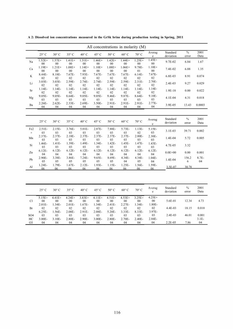
116

25° C 30° C 35° C 40° C 45° C 50° C 60° C 70° C

1.52E+ 1.57E+ 1.41E+ 1.51E+ 1.46E+ 1.42E+ 1.44E+ 1.25E+ 00 00 00 00 00 00 00 00

1.19E+ 1.21E+ 1.08E+ 1.14E+ 1.10E+ 1.08E+ 1.06E+ 9.78E- 00 00 00 00 00 00 00 01

8.44E- 8.18E- 7.67E- 7.93E- 7.67E- 7.67E- 7.67E- 6.14E- 02 02 02 02 02 02 02 02

3.03E- 3.03E- 2.59E- 2.74E- 2.74E- 2.59E- 2.59E- 2.31E- 02 02 02 02 02 02 02 02

1.14E- 1.14E- 1.14E- 1.14E- 1.14E- 1.14E- 1.14E- 1.14E- 02 02 02 02 02 02 02 02

9.05E- 9.05E- 8.64E- 9.05E- 9.05E- 9.46E- 9.87E- 8.64E- 03 03 03 03 03 03 03 03

2.26E- 2.62E- 2.33E- 2.69E- 3.50E- 2.91E- 2.91E- 2.91E- 04 04 04 04 04 04 04 04

Standard deviation

% error

2001 Data

9.7E-02 6.84 1.67

7.4E-02 6.88 1.35

6.8E-03 8.91 0.074

2.4E-03 9.27 0.029

1.9E-18 0.00 0.022

4.1E-04 4.31 0.018

3.9E-05 13.43 0.0003

25° C

30° C

35° C

40° C

45° C

50° C

60° C

70° C

5.15E+ 4.41E+ 4.24E+ 3.83E+ 4.11E+ 4.51E+ 4.53E+ 3.25E+ Cl 00 00 00 00 00 00 00 00

2.01E- 1.34E- 2.01E- 1.67E- 1.34E- 2.41E- 2.27E- 1.34E- Br 02 02 02 02 02 02 02 02

6.25E- 1.56E- 2.08E- 2.91E- 2.08E- 5.20E- 3.33E- 8.33E- SO4 03 03 03 03 03 03 03 03 HC 3.00E- 3.10E- 2.80E- 2.90E- 3.00E- 2.80E- 2.70E- 2.40E- O3 04 04 04 04 04 04 04 04

A 2: Dissolved ion concentrations measured in the GrSk brine during production testing in Spring, 2011

All concentrations in molarity (M)

Na

Ca

K

Li

Sr

Mg

Ba

Averag

e 1.45E+

00 1.10E+

00 7.67E-

02 2.70E-

02 1.14E-

02 9.10E-

03 2.77E-

04

25° C 30° C 35° C 40° C 45° C 50° C 60° C 70° C Averag e

Standard deviation

% error

2001 Data

Fe2 +

2.51E- 03

2.15E- 03

3.76E- 03

5.01E- 03

2.87E- 03

7.88E- 03

5.73E- 03

1.13E- 02

5.15E- 03 3.1E-03 39.71 0.002

Mn 2.37E- 03

Si 1.46E- 03

Zn 6.12E- 04

2.37E- 03

1.41E- 03

6.12E- 04

2.18E- 03

1.39E- 03

6.12E- 04

2.37E- 03

1.49E- 03

6.12E- 04

2.37E- 03

1.34E- 03

6.12E- 04

2.37E- 03

1.42E- 03

6.12E- 04

2.37E- 03

1.45E- 03

6.12E- 04

2.00E- 03

1.47E- 03

6.12E- 04

2.30E- 03 1.4E-04 5.72 0.005

1.43E- 03 4.7E-05 3.32

6.12E- 04 0.0E+00 0.00 0.001

Pb 2.90E- 05

Al 1.24E-

3.38E- 05

1.79E-

3.86E- 05

1.67E-

7.24E- 05

2.12E-

9.65E- 05

1.93E-

8.69E- 05

1.15E-

4.34E- 04

1.25E-

4.34E- 05

1.56E-

1.04E- 04 1.4E-04

1.59E-

156.2 6

8.7E- 04

3.5E-07 30.78 06 06 06 06 06 06 06 06 06

Averag e

4.25E+

Standard deviation

% error

2001 Data

00 5.6E-01 12.34 4.73 1.80E-

02 4.4E-03 18.15 0.010 3.97E-

03 2.4E-03 46.01 0.001 2.84E-

04 2.2E-05 7.86 3.1E-

04

117

A 3: Logsp vs. T vs. p data calculated by SupCrt for anhydrite, celestite and barite

Anhydrite

˚C

MPa 20 30 40 50 60 70 80 90 100 110 120 130 140 150

1 4.25 4.4 4.48 4.61 4.75 4.90 5.05 5.21 5.38 5.55 5.72 5.90 6.08 6.27 6 4.20 4.31 4.44 4.57 4.71 4.86 5.02 5.18 5.34 5.51 5.68 5.86 6.04 6.23

11 4.154 4.268 4.395 4.531 4.674 4.824 4.98 5.14 5.305 5.473 5.646 5.824 6.005 6.19 16 4.11 4.23 4.35 4.49 4.64 4.79 4.94 5.10 5.27 5.44 5.61 5.79 5.97 6.15 21 4.07 4.18 4.32 4.45 4.60 4.75 4.91 5.07 5.23 5.40 5.57 5.75 5.93 6.11 26 4.02 4.14 4.28 4.42 4.56 4.72 4.87 5.03 5.20 5.37 5.54 5.71 5.89 6.08

31 3.98 4.10 4.24 4.38 4.53 4.68 4.84 5.00 5.16 5.33 5.50 5.68 5.86 6.04 36 3.94 4.06 4.20 4.34 4.49 4.64 4.80 4.96 5.13 5.30 5.47 5.65 5.82 6.00 41 3.89 4.02 4.16 4.31 4.46 4.61 4.77 4.93 5.10 5.26 5.44 5.61 5.79 5.97

45 3.86 3.99 4.13 4.28 4.43 4.58 4.74 4.90 5.07 5.24 5.41 5.58 5.76 5.94

Celestite ˚C

MPa 20 30 40 50 60 70 80 90 100 110 120 130 140 150

1 5.65 5.69 5.75 5.82 5.90 6.00 6.10 6.21 6.33 6.46 6.59 6.73 6.88 7.03 6 5.61 5.65 5.71 5.78 5.86 5.96 6.06 6.18 6.30 6.42 6.55 6.69 6.84 6.99

11 5.56 5.61 5.67 5.74 5.83 5.92 6.03 6.14 6.26 6.38 6.52 6.65 6.80 6.95

16 5.52 5.56 5.63 5.70 5.79 5.89 5.99 6.10 6.22 6.35 6.48 6.62 6.76 6.91 21 5.48 5.52 5.59 5.66 5.75 5.85 5.95 6.07 6.19 6.31 6.44 6.58 6.72 6.87 26 5.43 5.48 5.55 5.63 5.71 5.81 5.92 6.03 6.15 6.28 6.41 6.55 6.69 6.83 31 5.39 5.44 5.51 5.59 5.68 5.78 5.88 6.00 6.12 6.24 6.37 6.51 6.65 6.80 36 5.35 5.40 5.47 5.55 5.64 5.74 5.85 5.96 6.08 6.21 6.34 6.48 6.62 6.76 41 5.31 5.36 5.43 5.52 5.61 5.71 5.82 5.93 6.05 6.18 6.31 6.44 6.58 6.73

45 5.27 5.33 5.40 5.49 5.58 5.68 5.79 5.90 6.02 6.15 6.28 6.42 6.56 6.70

Barite

˚C MPa 20 30 40 50 60 70 80 90 100 110 120 130 140 150

1 10.043 9.891 9.77 9.676 9.605 9.554 9.522 9.505 9.504 9.517 9.543 9.581 9.631 9.692 6 9.997 9.847 9.729 9.636 9.567 9.517 9.485 9.469 9.468 9.481 9.506 9.544 9.593 9.654

11 9.951 9.804 9.688 9.597 9.529 9.48 9.449 9.433 9.432 9.445 9.47 9.508 9.556 9.616 16 9.905 9.762 9.648 9.559 9.492 9.444 9.413 9.398 9.397 9.41 9.435 9.472 9.52 9.579 21 9.86 9.72 9.608 9.521 9.455 9.408 9.378 9.363 9.363 9.376 9.401 9.437 9.485 9.543 26 9.816 9.679 9.569 9.483 9.419 9.373 9.343 9.329 9.329 9.342 9.367 9.403 9.45 9.507 31 9.773 9.638 9.53 9.446 9.383 9.338 9.309 9.296 9.296 9.309 9.333 9.369 9.415 9.472 36 9.73 9.598 9.492 9.41 9.348 9.304 9.276 9.262 9.263 9.276 9.3 9.336 9.382 9.438 41 9.687 9.558 9.455 9.374 9.313 9.27 9.242 9.23 9.23 9.243 9.268 9.303 9.349 9.404 45 9.654 9.527 9.425 9.345 9.285 9.243 9.216 9.204 9.205 9.218 9.242 9.277 9.323 9.378

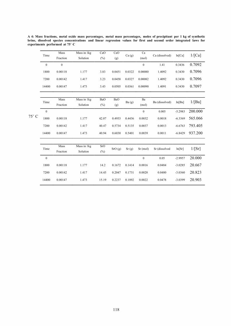
118

Time Mass

Fraction

Mass in 1kg

Solution

BaO

(%)

BaO

(g)

Ba (g) Ba

(mol)

Ba (dissolved)

ln[Ba] 1/[Ba]

0 0 0.005 -5.2983 200.000

1800

0.00118

1.177

42.07

0.4953

0.4436

0.0032

0.0018

-6.3369 565.066

7200 0.00142 1.417 40.47 0.5734 0.5135 0.0037 0.0013 -6.6763 793.405

14400 0.00147 1.473 40.94 0.6030 0.5401 0.0039 0.0011 -6.8429 937.200

A 4: Mass fractions, metal oxide mass percentages, metal mass percentages, moles of precipitant per 1 kg of synthetic brine, dissolved species concentrations and linear regression values for first and second order integrated laws for experiments performed at 75˚ C

Time Mass

Fraction

Mass in 1kg

Solution

CaO

(%)

CaO

(g)

Ca (g) Ca

(mol)

Ca (dissolved)

ln[Ca] 1/[Ca]

0 0 0 1.41 0.3436 0.7092

1800

0.00118

1.177

3.83

0.0451

0.0322

0.00080

1.4092

0.3430 0.7096

7200

0.00142

1.417

3.23

0.0458

0.0327

0.00082

1.4092

0.3430 0.7096

14400 0.00147 1.473 3.43 0.0505 0.0361 0.00090 1.4091 0.3430 0.7097

75˚ C

Time Mass

Fraction

Mass in 1kg

Solution

SrO

(%)

SrO (g)

Sr (g)

Sr (mol)

Sr (dissolved

ln[Sr] 1/[Sr]

0 0 0.05 -2.9957 20.000

1800 0.00118 1.177 14.2 0.1672 0.1414 0.0016 0.0484 -3.0285 20.667

7200 0.00142 1.417 14.45 0.2047 0.1731 0.0020 0.0480 -3.0360 20.823

14400 0.00147 1.473 15.19 0.2237 0.1892 0.0022 0.0478 -3.0399 20.903

119

Mass Mass in 1kg CaO CaO Ca Time

Fraction

Solution

(%)

(g) Ca (g)

(mol) Ca (dissolved) ln[Ca] 1/[Ca]

0 0 0 1.41 0.3436 0.7092 1800 0.00083 0.8343 4.07 0.0340 0.0243 0.0006 1.4094 0.3432 0.7095

7200 0.00118 1.1829 3.5 0.0414 0.0296 0.0007 1.4093 0.3431 0.7096

14400 0.00132 1.3219 3.2 0.0423 0.0302 0.0008 1.4092 0.3431 0.7096

Time

Mass

Fraction

Mass in 1kg

Solution

BaO

(%)

BaO

(g)

Ba (g)

Ba

(mol)

Ba (dissolved)

ln[Ba]

1/[Ba]

0 0 0.00500 -5.2983 200.000 1800 0.00083 0.8343 37.27 0.3109 0.2785 0.0020 0.00297 -5.8185 336.466

7200 0.00118 1.1829 37.19 0.4399 0.3940 0.0029 0.00213 -6.1513 469.316

14400 0.00132 1.3219 38.38 0.5073 0.4544 0.0033 0.00169 -6.3824 591.337

Fraction Solution (%) (g)

0 0 0.05 -2.9957 20.000 1800 0.00083 0.8343 17.73 0.1479 0.1251 0.0014 0.0486 -3.0247 20.588

7200 0.00118 1.1829 17.92 0.2120 0.1792 0.0020 0.0480 -3.0375 20.853

14400 0.00132 1.3219 17.79 0.2352 0.1989 0.0023 0.0477 -3.0422 20.951

A 5: Mass fractions, metal oxide mass percentages, metal mass percentages, moles of precipitant per 1 kg of synthetic brine, dissolved species concentrations and linear regression values for first and second order integrated laws for experiments performed at 150˚ C

150˚ C

Time Mass Mass in 1kg SrO SrO

Sr (g) Sr (mol) Sr (dissolved ln[Sr] 1/[Sr]

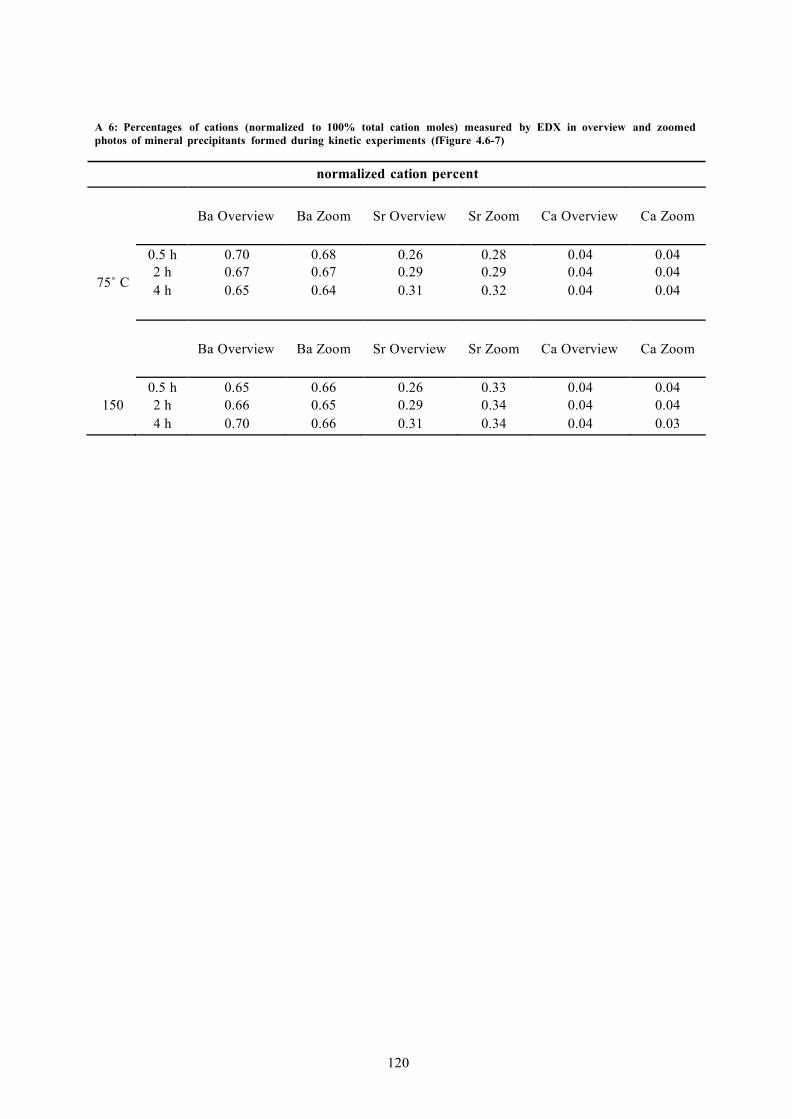
120

A 6: Percentages of cations (normalized to 100% total cation moles) measured by EDX in overview and zoomed photos of mineral precipitants formed during kinetic experiments (fFigure 4.6-7)

normalized cation percent

75˚ C

Ba Overview

Ba Zoom

Sr Overview

Sr Zoom

Ca Overview

Ca Zoom

0.5 h 0.70 0.68 0.26 0.28 0.04 0.04 2 h 0.67 0.67 0.29 0.29 0.04 0.04 4 h 0.65 0.64 0.31 0.32 0.04 0.04

Ba Overview

Ba Zoom

Sr Overview

Sr Zoom

Ca Overview

Ca Zoom

0.5 h 0.65 0.66 0.26 0.33 0.04 0.04 150 2 h 0.66 0.65 0.29 0.34 0.04 0.04

4 h 0.70 0.66 0.31 0.34 0.04 0.03

121

Wl "

Appendix B: Selected photomicrographs of experimentally formed alkali earth metal su lfate mineral precipitants

' Ao .- ..'""'"" l I I """' l loo l"p '>01'1 V ''' ""' II \I l

1-----i V•'l'' 1 '.01 11/o n'l•lll• 111/llv'"'

B 1:Barite precipitated from a 5 molal Naa solution.

122

ll'on 1\r btlt>db:>l•nd II J n>m Ho<lnp • 70 00 V n•lA ':it/ H Vmtjt <tli mu nq · I 'III II: X Hnt dRnr oo\l• 1JIJ II ""

B 2: Celestite precipitated from a 5 molal Naa solution.

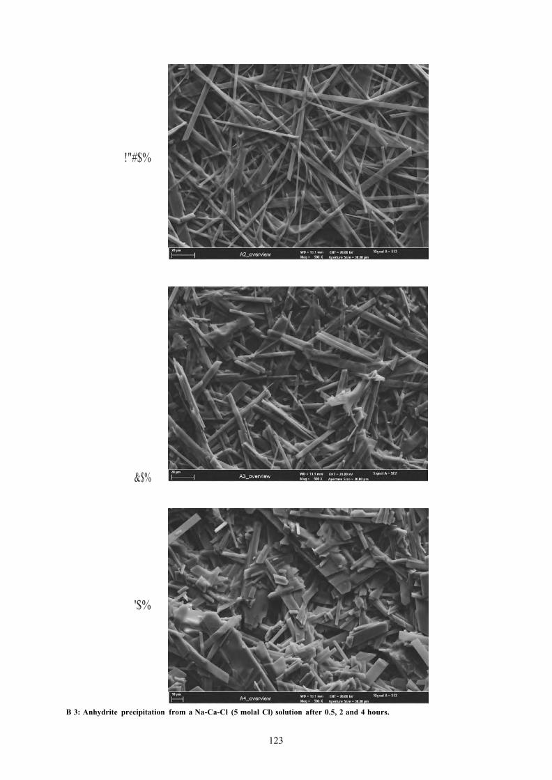
123

!"#$%

&$%

'$%

B 3: Anhydrite precipitation from a Na-Ca-Cl (5 molal Cl) solution after 0.5, 2 and 4 hours.

124

/ ''""

1 !I

Art.r r-.1..,, .,,.. llr"'" l hr <h.,. M I"''1" 111 ...11

H V r•upu lr•" "Hl I l(X IUr-ndl'r.rJruA r (Ill!""

r. !1 IHh>!"1<1 j 4 1!!1!! ' lll " l IUti •V ...II II t , , ; t-----1 >l••l ' .,., q 411'."1 r " rlqr.,ro.• 30001JTT

B 4: Strontio-barite with anhydrite precipitated from a mixed electrolyte (Na-Ca-Ba-Sr-O-S04-H20; 5 molal Cl) solution at GrSk concentrations.

125

)'"'

\m /ubo < t>.b, -.I Atu[ '• ''"" " )i,,,,'f' '•1111 hV '-"I ">IA \!) V<'f<jf <>1. t>fU!UJ II I!I I'IX Hl •ll dAI\/6 Rk I JI:I [I/1\

lub• ll '1lnu f l •, 'l '""' li »< l<>!l' •,{10 kV <;., l"d l A <;!'

f-------------- V• fl[fl>< HJII<t If 1'1 X lil <'f< dltl\1[161\" f':ll( jUI\

B4 coot: Strontio.-barite with anhydrite precipitated from a mixed electrolyte (Na-Ca-Ba-Sr-CI-S04-H20; 5 molal 0) solution at GrSk concentrations.