suitability of different mean speeds for model-based ...bdeschutter/pub/rep/07_029.pdf ·...
TRANSCRIPT
Delft University of Technology
Delft Center for Systems and Control
Technical report 07-029
Suitability of different mean speeds for
model-based traffic control∗
M. Burger, A. Hegyi, and B. De Schutter
If you want to cite this report, please use the following reference instead:
M. Burger, A. Hegyi, and B. De Schutter, “Suitability of different mean speeds for
model-based traffic control,” Proceedings of the 87th Annual Meeting of the Trans-
portation Research Board, Washington, DC, 18 pp., Jan. 2008. Paper 08-2010.
Delft Center for Systems and Control
Delft University of Technology
Mekelweg 2, 2628 CD Delft
The Netherlands
phone: +31-15-278.51.19 (secretary)
fax: +31-15-278.66.79
URL: http://www.dcsc.tudelft.nl
∗This report can also be downloaded via http://pub.deschutter.info/abs/07_029.html

Burger, Hegyi, De Schutter 1
Suitability of different mean speeds for model-based traffic control
Submission date: November 12, 2007
Word count: 5796 words + (5 figures + 1 tables)*(250 words) = 7296 words
Authors:
M. Burger, Delft Center for Systems and Control, Delft University of Technology, Mekelweg 2, 2628 CD
Delft, The Netherlands, phone: +31-15-278.65.24, fax: +31-15-278.66.79, email: [email protected]
A. Hegyi, Transport and Planning, Delft University of Technology, P.O. Box 5048, 2600 GA, Delft, The
Netherlands, phone: +31-15-278.20.87, fax: +31-15-278.69.09, email: [email protected]
B. De Schutter, Delft Center for Systems and Control, Delft University of Technology, Mekelweg 2, 2628
CD Delft, The Netherlands, phone: +31-15-278.51.13, fax: +31-15-278.66.79, email: [email protected]
Burger, Hegyi, De Schutter 2
Abstract.
Traffic jams are an economic and environmental problem in many countries. When traffic demand exceeds
the freeway capacity, shock waves can be caused by small disturbances in the traffic flow. Since it is not
always desirable or feasible to add more lanes on freeways to overcome capacity problems, alternative
methods have been developed to reduce and to dissolve traffic jams. One of these methods is using model-
based traffic control.
The model-based methods use traffic flow models, in which the speeds are typically space mean
speeds, while the measured speeds on a freeway are often time mean speeds (measured by loop detectors).
The difference between using space mean speeds and time mean speeds for model-based methods has not
yet been addressed in literature. In this paper, we investigate the possible performance loss caused by using
another mean speed type than the space mean speed for model-based traffic control.
Methods for approximating the space mean speed based on local measurements are discussed, to-
gether with the time mean speed and geometric mean speed. The suitability of six mean speed types is
investigated using microscopic simulation. Next, the three most suitable mean speed types for model-based
traffic control are used to determine dynamic speed limits on a freeway using a model predictive control
approach. All three types of mean speeds result in the resolution of the congestion in the test scenario and
lead to a performance improvement of about 14%.

Burger, Hegyi, De Schutter 3
1 INTRODUCTION
In many countries, the demand on freeways exceeds the capacity almost every day, which can lead to traffic
jams due to disturbances in the traffic flow. Increasing the number of lanes on a freeway is one approach
to address this problem. However, if this solution is infeasible or not desired, more advanced solutions
are necessary. A potential solution is model-based traffic control, which is capable of reducing or even
dissolving upstream propagating shock waves.
In the literature, two control approaches using speed limits can be found. The first approach is
based on homogenization of the traffic flow (1–3), and the second approach focuses on flow limitation to
solve traffic jams (4–6). The basic idea for homogenization is the reduction of speed differences, thereby
increasing the stability (and safety) of the traffic flow. Using flow limitation, the traffic is slowed down
upstream of a traffic jam, thereby reducing the inflow of the traffic jam, which will reduce the length of the
traffic jam. We use the second approach, since it is more suitable for reducing shock waves. In simulation
studies (6, 7) it has been shown that a shock wave can be resolved by holding back the upstream traffic (via
dynamic speed limits) that is feeding it.
Loop detectors are used to measure the traffic state on the freeway, typically counting the number
of passing vehicles, and determining the mean speed over a certain time. There are many ways to determine
mean speeds. For traffic on freeways, usually the time mean speed and space mean speed are used. Assuming
the freeway is equipped with the necessary sensors and measurement equipment, the time mean speed can
be calculated using the arithmetic mean of the measured vehicle speed on a given location. The space mean
speed can be estimated using the harmonic mean of the measured vehicle speeds on a given location. In
addition, this paper introduces the geometric mean of the vehicle speeds, which complements the arithmetic
and harmonic mean as the third ‘classic’ Pythagorean mean (8).
When it is possible to measure speeds instantaneously (e.g., by using cameras), the space mean
speed for a time interval can be obtained by using the average space mean speed over multiple measurements.
Since often it is not possible to obtain instantaneous vehicle speeds, we focus on mean speeds obtained by
using spot measurements (e.g., by using loop detectors). The space mean speed is based on instantaneous
vehicle speeds, and an approximation method is needed. We discuss several approximation methods for
obtaining space mean speeds, based on local measurements. In total, six methods for calculating mean
speeds are discussed, as well as their suitability for use in model-based traffic control.
In this paper Model Predictive Control (MPC) is used to determine dynamic speed limits on a part
of the Dutch freeway A12. The objective of the traffic controller is to reduce the travel time. If the traffic
jams are solvable, this will result in resolved shock waves, since the lowest travel times are obtained when
the congestion is resolved on the freeway (7). The advantage of MPC for this application is that due to the
receding horizon strategy of MPC, the controller can take actions that increase the travel time for a short
period (slowing vehicles down), when this is beneficial over a large period (reducing the shock wave). The
current traffic state is used as initial value to predict the future traffic states.
This paper is organized as follows. In Section 2 six ways of calculating mean speeds are discussed.
These mean speeds will be used to describe the states of the traffic flow. We examine which mean speed
variant is the most suitable for model-based traffic control, for reducing shock waves on the freeway. Shock
waves are the topic of Section 3, where it is also discussed how dynamic speed limits can reduce shock
waves. In Section 4 we explain how MPC can be used to determine speed limits, such that shock waves
will be reduced. The resulting traffic control approach is discussed in Section 5, where the criteria for the
suitability of the mean speed variants are given. The prediction model used for MPC is discussed in Section
6, together with the program used to simulate the traffic network. Details of the experiment are given in
Section 7, followed by the results of the experiment in Section 8. The conclusions are discussed in Section
9.

Burger, Hegyi, De Schutter 4
2 VARIOUS MEAN SPEEDS
In the field of freeway traffic modelling, two mean speeds are often used: time mean and space mean
speeds (9, 10). Time mean speeds are based on measurements on a given location, and are averaged over
a certain time span. These speeds can be measured by, e.g., loop detectors. Space mean speeds are based
on measurements over a certain length of the freeway, at a given time instant. Video images can be used to
obtain space mean speeds (11).
Macroscopic traffic flow models use space mean speeds, while in practice, the vehicle speeds are in
general measured by loop detectors. These are unable to deliver exact space mean speeds, and estimations
are needed.
To the authors’ best knowledge, no literature discussing the performance of different mean speeds
for model-based traffic control is available. In the research reported in this paper, loop detectors are used
to obtain the traffic state. The loop detectors measure individual vehicle speeds uL, at a location xmsr over a
sample time period Ts, where the subscript L is used to indicate that the measurement is done locally. These
measurement moments at location xmsr,2 are visualized in the time-space diagram in Figure 1, using circles.
x
t
Lm
Ts
uL,1 uL,2 uL,3 uL,4
uI,1
uI,2
uI,3
uI,4xmsr,1
xmsr,2
ksTs (ks +1)Ts
FIGURE 1 Time-space diagram, containing the measurement area, and vehicle trajectories (dashed
lines).
The space mean speed can be determined by averaging the individual vehicle speeds uI, measured
at a time instant ksTs, where the subscript I indicates that the measurement is done instantaneously. This is
shown in Figure 1 at sample step ks, where the squares are the measurement locations.
Using loop detectors, the outflow of the traffic at location xmsr,2 can be obtained by dividing the
number of observed vehicles N(ks) leaving the freeway segment [xmsr,1,xmsr,2] in the time interval [ksTs,
(ks+1)Ts), by the sampling time interval Ts. Hence, the average outflow for the time interval [ksTs, (ks+1)Ts)
can be determined using
q(ks) =N(ks)
Ts
. (1)
The density follows from the outflow q(ks), the space mean speed v(ks), and the number of lanes λm on a
freeway link m, as
ρ(ks) =q(ks)
v(ks)λm
(2)

Burger, Hegyi, De Schutter 5
The space mean speed can be approximated using six different methods, which are discussed below. These
methods will be used to calculate the mean speed. Together with the density, which is computed using (1)
and (2), these variables will be used to describe the state of the traffic flow.
2.1 Time Mean Speed
The time mean speed is calculated using the arithmetic mean of the N(ks) individual vehicle speeds uL,l
measured over an interval [ksTs,(ks +1)Ts) (where Ts is the sampling period) as (9)
vtms(ks) =1
N(ks)
N(ks)
∑l=1
uL,l (3)
In the time-space diagram shown in Figure 1, the measurements of the vehicle speeds are shown as circles.
Loop detectors typically provide the time mean speed.
2.2 Estimated Space Mean Speed
For obtaining the estimated space mean speed, the harmonic mean of the locally measured vehicle speeds
is used by (9), given as
vsms(ks) =
(
1
N(ks)
N(ks)
∑l=1
1
uL,l
)−1
(4)
This equation gives the exact space mean speed when the speed distribution over time and space is homo-
geneous. In practice this never holds exactly, and the equation yields an estimate of the actual space mean
speed.
In Figure 1, this estimated space mean speed calculation is shown graphically. Assuming the lo-
cally measured vehicle speeds uL measured at xmsr,2 are constant, the vehicle trajectories can be extended as
straight lines, where the slope equals the speed. The measurements that would be ideally used for determin-
ing the space mean speed are shown as the squares at sample step ks.
2.3 Geometric Mean Speed
Besides the arithmetic and harmonic mean, there is a third Pythagorean mean, namely the geometric mean
(8). This mean can be calculated as
vgeo(ks) =N(ks)
√√√√
N(ks)
∏l=1
uL,l (5)
The geometric mean is often used in economics, but an interpretation of the value for traffic has not
been found in literature. In general, the relation between the harmonic mean H(x), geometric mean G(x),and arithmetic mean A(x) is H(x)≤ G(x)≤ A(x) for a array x of positive numbers, where equality is reached
if, and only if all numbers in x are equal (8). For traffic, this means that the geometric mean speed is always
larger than or equal to the space mean speed, and smaller than or equal to the time mean speed.
2.4 Estimated Space Mean Speed Using Instantaneous Speed Variance
A method for estimating the space mean speed, based on instantaneous speeds, is proposed in (12). It uses
the relation between time mean speed vtms (as given by (3)), and the space mean speed vsms:
vtms(ks) =σ2
sms(ks)
vsms(ks)+ vsms(ks) (6)

Burger, Hegyi, De Schutter 6
where σ2sms(ks) is the speed variance for the instantaneously measured vehicle speeds. From this equation
the space mean speed can be determined as
vsms(ks) =1
2
{
vtms(ks)+√
v2tms(ks)−4σ2
sms(ks)
}
Since the instantaneous speed variance σ2sms(ks) cannot be determined by local measurements, an estimation
is used, given by
σ2sms(ks) =
1
2N(ks)
N(ks)
∑l=1
vsms(ks)
uL,i(uL,l+1 −uL,l)
2
where vsms(ks) is the harmonic mean speed (4), and the estimated space mean speed becomes
vsms,I(ks) =1
2
{
vtms(ks)+√
v2tms(ks)−4σ2
sms(ks)
}
(7)
2.5 Estimated Space Mean Speed Using Local Speed Variance
In (13), an estimate of the space mean speed is proposed, based on the local mean speed and the local speed
variance of the measured speeds. The estimated space mean speed is determined by
vsms,L(ks) = vtms(ks)−σ2
tms(ks)
vtms(ks)(8)
where vtms(ks) is calculated using (3), and
σ2tms(ks) =
1
N(ks)
N(ks)
∑l=1
(uL,l − vtms(ks))2 =
1
N(ks)
(N(ks)
∑l=1
u2L,l
)
− v2tms(ks) (9)
2.6 Time Average Space Mean Speed
Now we consider a finer sampling of with a sample period Tt such that Tt = Ts/Mt for some positive integer
Mt. Using, e.g., video images, it is possible to obtain the space mean speed vsms(kt) on a freeway segment
for every sample step kt in the interval [ktTt,(kt +Mt)Tt) = [ksTs,(ks + 1)Ts) (11). Since the space mean
speed is defined on a certain time instant over a certain freeway stretch, and the previous five mean speed
measures are defined on a certain position on the freeway over a given time period, the mean speed types
are not directly comparable. In the latter cases a time average of the space mean speed is used to represent
the actual space mean speed. Therefore, we now define a mean speed that is a time average of the obtained
space mean speeds in the time period [ktTt, (kt+Mt)Tt):
vsms(ks) =1
Mt
kt+Mt−1
∑κ=kt
vsms(κ) (10)
where kt = Mtks.
3 SHOCK WAVES
Shock waves are upstream propagating traffic jams on freeways, which often emerge from on-ramps and
other types of bottlenecks. The outflow of a shock wave is typically around 70% of the freeway capacity
(14), and resolving these shock waves can greatly improve the freeway traffic flow. Since the vehicle speeds

Burger, Hegyi, De Schutter 7
in the shock wave are low, travel times are higher than in the free flow situation. Shock waves also cause
potentially dangerous situations due to speed differences, and air pollution is increased by slowly driving
and frequently accelerating and braking vehicles.
Shock waves can be reduced or dissolved by applying dynamic speed limits (7). Traffic upstream
of the shock wave can be slowed down, thereby limiting the inflow to the shock wave. This will reduce
the length of the shock wave, and using dynamic speed limits can even dissolve the shock wave (depending
on the traffic demand and length of the freeway stretch where dynamic speed limits are used). The settings
for the dynamic speed limits can, e.g., be determined using MPC (6), which is also used in the research
discussed in this paper.
4 MODEL PREDICTIVE CONTROL
Let Tc denote the control sample period and let kc be the corresponding control sample counter.
We use the MPC scheme to solve the problem of optimal coordination of dynamic speed limits, as
shown in Figure 2. MPC uses a model to describe the physical system. This model allows to predict future
states of the system, and it takes the effect of applying control actions into account. Using an optimization
method, the values of the control variables resulting in the best performance are determined. The future
states are predicted up to a prediction horizon of Np controller steps ahead. Often a control horizon of Nc
steps is used, where Nc < Np. The control variables are then optimized up to the control horizon, and after
the control horizon the control variables vctr remain constant. The control horizon is mostly used to reduce
the amount of variables to optimize, thereby reducing the calculation time for the optimization.
Once the optimal values for the objective are computed, the control actions for the first controller
step kc are applied to the physical system, and the optimization is repeated for the next controller step kc+1.
This method of shifting the horizon for which control variables are optimized, is often called receding
horizon.
traffic demand
control input:
speed limits
expected demand
traffic system
rolling horizon
controller
optimization
traffic state:
speed, flow,
density
prediction
vctr,m,i(kc)
(Np,Nc)
(each kc)
J(kc)
FIGURE 2 Schematic overview of the model predictive traffic control structure.
In this paper, the controlled system is the traffic network, from which measurements are taken. The
obtained mean speeds, flows, and densities are sent to the controller at each controller step kc. The controller
uses a macroscopic traffic model to predict the future traffic states over a prediction horizon of Np controller
steps. Using numerical optimization, the optimal speed limits vctr,m,i are determined up to a control horizon
Burger, Hegyi, De Schutter 8
of Nc controller steps, where m is the link index, and i is the segment index on that link (see Section 6 for
more details).
5 APPROACH
We investigate the effect of using different mean speeds instead of space mean speeds in the MPC prediction
model. The control goal is to reduce shock waves, by applying dynamic speed limits on a freeway. A mi-
croscopic traffic simulator is used as traffic network, which allows us to measure individual vehicle speeds,
and to calculate the various mean speeds discussed in Section 2.
5.1 Objective for Dynamic Speed Limit Control
The desired effect of applying control is reducing shock waves on freeways. We use MPC, with the mini-
mization of the total time vehicles spend in the area of the traffic network under consideration as an objective.
The Total Time Spent (TTS) for one control sample period Tc can be calculated as the sum of vehicles per
segment (ρm,i(κ)λm,iLm), plus the amount of vehicles wo(κ) that were unable to enter the area under consid-
eration due to congestion. The numerical optimization is searching for a minimum value for the Total Time
Spent (TTS) by the vehicles over the prediction horizon Np in the controlled area of the network:
JTTS(kc) = Tc
kc+Np−1
∑κ=kc
{
∑(m,i)∈M
ρm,i(κ)λm,iLm + ∑o∈O
wo(κ)
}
(11)
where M is the set of links and segments, O is the set of origins for the measured areas, ρm,i(κ) is the
average density in segment i of link m at controller step κ , and wo(κ) is the number of vehicles waiting in a
queue to enter the freeway at controller step κ , due to congestion.
In order to avoid large speed limit differences between adjacent segments, a second objective func-
tion is also taken into account. It calculates the average of the sum of the squared difference between two
speed limits vctr, for the entire prediction horizon Np:
JSLD(kc) =1
NmNp
Nm
∑m=1
1
Nctr,m −1
kc+Np−1
∑κ=kc
Nctr,m−1
∑i=1
(vctr,m,i+1(κ)− vctr,m,i(κ))2
(12)
where Nm is the number of links, Nctr,m is the number of controlled segments on link m, and vctr,m,i(κ) is the
dynamic speed limit applied in segment i of link m at controller step κ .
The two objective functions are combined as
J(kc) = JTTS(kc)+ζ JSLD(kc) (13)
where ζ is a weighting factor.
5.2 Performance Criterion for Model Calibration
Since the model parameters in a traffic model are different for each traffic network, model calibration is
necessary. This is done by offline numerical optimization using an objective function given by
Jcal(θ) =Ks−McNp
∑ks=1
Jcal(ks,θ) (14)

Burger, Hegyi, De Schutter 9
where θ is the set of model parameters, Ks is the number of sample steps ks for which measurement data is
available, Mc is a positive integer value relating the controller steps and sample steps as ks = Mckc (and thus
Tc = McTs), and Jcal(ks,θ) is given by
Jcal(ks,θ) =
[
1
McNp
ks+McNp−1
∑κ=ks
∑(m,i)∈M
{(vm,i(κ)− vm,i(κ,θ)
v(ks)
)2
+
(ρm,i(κ)− ρm,i(κ,θ)
ρ(ks)
)2}] 1
2
(15)
where v(ks) and ρ(ks) are the average speed and flow of the measured data from simulation step ks to
ks+McNp. A lower value of the objective function (14) implies a better fit of the predicted states {vm,i(·,θ),ρm,i(·,θ)} by a macroscopic model on the measured states {vm,i,ρm,i}. Since the traffic controller will
be optimizing on the TTS, also the difference in measured and predicted TTS is determined, to judge the
performance of the parameter values. The error is given by
ETTS(θ) =1
Kc −Np
Kc−Np
∑kc=1
JTTS(kc,θ)− JTTS(kc)
JTTS(kc)(16)
which gives the average percentage of mismatch between the TTS of the measured data JTTS(kc) and the
predicted data JTTS(kc,θ) for the parameter set θ , where Kc is the total number of control steps kc in the
simulation.
The six variants for calculating the mean speed vm,i(k) (equations (3)-(10)) are used to calibrate a
macroscopic model. Using (14) we can determine how well the model can predict future states (mean speeds
and densities), using the different mean speed variants. Using (16), the difference between the measured
and predicted TTS can be determined.
To increase the reliability of the results, the calibration is done using a multi-start optimization
approach for the values of the model parameter vector σ . From this calibration, the parameter set resulting
in the lowest value of Jcal(θ) is used for determining both Jcal(θ) and ETTS(θ) on 5 data sets, each created
with a different random seed, to account for the stochasticity of the microscopic simulation model. The
same data sets are used for all mean speed types to have a fair comparison of the results. From these 5
values of Jcal(θ) and ETTS(θ), the average values Jcal(θ) and ETTS(θ) are used to compare the performance
of the different mean speeds.
6 TRAFFIC FLOW MODELLING
6.1 Prediction Model
For the prediction of future traffic states, a macroscopic traffic model is used to reduce computation time.
Any macroscopic traffic model can be used for the prediction. For the research we report on in this paper, the
METANET traffic flow model is used, which is described in e.g. (15). Here we will give a brief description
of the model, including the extensions proposed by Hegyi et al. (6).
The METANET model divides a freeway network into multiple links m. A link is divided into
multiple segments i, for which the state is given in terms of the density ρm,i(k), space mean speed vm,i(k),and outflow qm,i(k) of the segment. Here k denotes the simulation step, with simulation time interval T . The
relation between the simulation time interval T and sampling time interval Ts is assumed to be given by
Ts = MsT (17)
where Ms is a positive integer.
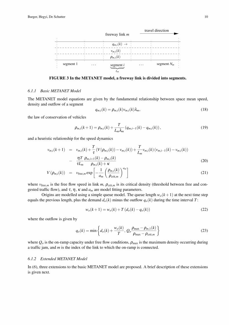
Figure 3 shows a link m which is divided into Nm segments. Each segment has a length Lm, and a
number of lanes λm, which are constant for all segments in a link m.
Burger, Hegyi, De Schutter 10
travel directionfreeway link m
. . .. . .segment 1 segment i︸ ︷︷ ︸
Lm
segment Nm
qm,i(k) →
ρm,i(k)
vm,i(k)
FIGURE 3 In the METANET model, a freeway link is divided into segments.
6.1.1 Basic METANET Model
The METANET model equations are given by the fundamental relationship between space mean speed,
density and outflow of a segment
qm,i(k) = ρm,i(k)vm,i(k)λm, (18)
the law of conservation of vehicles
ρm,i(k+1) = ρm,i(k)+T
Lmλm
(qm,i−1(k)−qm,i(k)) , (19)
and a heuristic relationship for the speed dynamics
vm,i(k+1) = vm,i(k)+T
τ(V (ρm,i(k))− vm,i(k))+
T
Lm
vm,i(k)(vm,i−1(k)− vm,i(k))
−ηT
τLm
ρm,i+1(k)−ρm,i(k)
ρm,i(k)+κ(20)
V (ρm,i(k)) = vfree,m exp
[
−1
am
(ρm,i(k)
ρcrit,m
)am]
(21)
where vfree,m is the free flow speed in link m, ρcrit,m is its critical density (threshold between free and con-
gested traffic flow), and τ , η , κ and am are model fitting parameters.
Origins are modelled using a simple queue model. The queue length wo(k+1) at the next time step
equals the previous length, plus the demand do(k) minus the outflow qo(k) during the time interval T :
wo(k+1) = wo(k)+T (do(k)−qo(k)) (22)
where the outflow is given by
qo(k) = min
{
do(k)+wo(k)
T, Qo
ρmax −ρm,1(k)
ρmax −ρcrit,m
}
(23)
where Qo is the on-ramp capacity under free flow conditions, ρmax is the maximum density occurring during
a traffic jam, and m is the index of the link to which the on-ramp is connected.
6.1.2 Extended METANET Model
In (6), three extensions to the basic METANET model are proposed. A brief description of these extensions
is given next.

Burger, Hegyi, De Schutter 11
The first extension adds the effect of using dynamic speed limits to the METANET model. The
desired speed V (ρm,i)(k) in (20) is replaced by
Vext(ρm,i(k)) = min{(1+α)vctr,m,i(k), V (ρm,i)(k)} (24)
where α is the non-compliance factor to the speed limits, and vctr,m,i(k) is the applied speed limit on segment
i of link m at time step k.
The second extension is introduced to model the inflow of traffic at mainstream origins. The origin
o of link m is limited by either the demand, or the maximum inflow, given as
qo(k) = min
{
do(k)+wo(k)
T, qlim,m,1(k)
}
(25)
where the maximum inflow qlim,m,1(k) is dependent on the limiting speed in the first segment of link m:
qlim,m,1(k) =
{
γqspd,m(k) if vlim,m,1(k)<V (ρcrit,m)
γqcap,m if vlim,m,1(k)≥V (ρcrit,m)
where γ is a model fitting parameter, and
qcap,m = λmVext(ρcrit,m)ρcrit,m
qspd,m(k) = λmvlim,m,1(k)ρcrit,mam
√
−am ln
(vlim,m,1(k)
vfree,m
)
and
vlim,m,1(k) = min{vctr,m,1(k), vm,1(k)}
When the origin is an on-ramp, (23) is used.
The third extension improves the modelling of shock waves travelling upstream on the link. The
anticipation behavior of drivers may be different at the head and tail of a traffic jam. The anticipation
constant η in (20) is replaced by the density-dependent parameter
ηm,i(k) =
{
ηhigh if ρm,i+1(k)≥ ρm,i(k)
ηlow if ρm,i+1(k)< ρm,i(k)(26)
in order to account for these anticipation differences.
6.2 Traffic simulation
The physical traffic network is simulated using a microscopic simulation program. Any traffic microscopic
simulation program can be used. For the research discussed in this paper, Paramics v5.1 by Quadstone
(16) is used to represent the traffic network. A plug-in is created to gather data from loop detectors in
the simulation, and to compute the mean speeds discussed in Section 2. The speed limits on the controlled
segments are changed, according to the results of the traffic controller. The resulting speed limits are rounded
to the nearest multiple of 10 between 40 and 120 [km/h].

Burger, Hegyi, De Schutter 12
7 EXPERIMENT
7.1 Traffic Network Layout
For the traffic network, a part of the Dutch freeway A12 is implemented in Paramics. The stretch of interest
is the part between Veenendaal and Maarsbergen, which is a freeway stretch without on-ramps and off-
ramps. The loop detectors in the micro-simulator are placed at the locations of the existing loop detectors on
the freeway. Since the distance between subsequent loop detectors is varying, the model consists of multiple
links m, all containing one segment. The links are chosen such that the detectors are near the downstream
boundary, in order to obtain accurate measurements of the outflow q of the links. The link lengths vary
between 545 [m] and 810 [m], and the total length of the measured area is 17422 [m]. Links are grouped in
freeway sections of about 2 [km], where the dynamic speed limits are assumed to be the same.
7.2 Traffic Scenario
The traffic demand qdem on the freeway is assumed to be known, and to be constant, equalling 4400[veh/h].This is chosen such that the shock wave will remain existent when no control is applied. A shock wave is
introduced by simulating an incident downstream of the controlled area. One vehicle is stopped for a period
of 5 minutes, during which one of the two lanes is blocked. This creates a traffic jam, which expands while
the lane is blocked, and the resulting shock wave moves upstream when both lanes are accessible again.
FIGURE 4 Traffic condition without control.
Figure 4 shows the measurements on the network. On the horizontal axis, the time is shown, and on
the vertical axis, the segment indices are given. The traffic flows from bottom to top. The first subplot shows
the speed limits, which are all 120 [km/h], since no control is applied. In the second subplot, the measured
mean speeds are given, obtained using (5). Lighter colours represent higher mean speeds. The shock wave
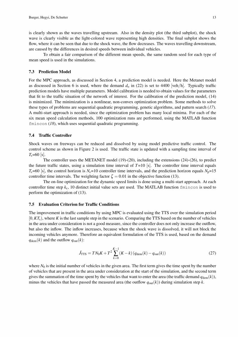
Burger, Hegyi, De Schutter 13
is clearly shown as the waves travelling upstream. Also in the density plot (the third subplot), the shock
wave is clearly visible as the light-colored wave representing high densities. The final subplot shows the
flow, where it can be seen that due to the shock wave, the flow decreases. The waves travelling downstream,
are caused by the differences in desired speeds between individual vehicles.
To obtain a fair comparison of the different mean speeds, the same random seed for each type of
mean speed is used in the simulations.
7.3 Prediction Model
For the MPC approach, as discussed in Section 4, a prediction model is needed. Here the Metanet model
as discussed in Section 6 is used, where the demand do in (22) is set to 4400 [veh/h]. Typically traffic
prediction models have multiple parameters. Model calibration is needed to obtain values for the parameters
that fit to the traffic situation of the network of interest. For the calibration of the prediction model, (14)
is minimized. The minimization is a nonlinear, non-convex optimization problem. Some methods to solve
these types of problems are sequential quadratic programming, genetic algorithms, and pattern search (17).
A multi-start approach is needed, since the optimization problem has many local minima. For each of the
six mean speed calculation methods, 100 optimization runs are performed, using the MATLAB function
fmincon (18), which uses sequential quadratic programming.
7.4 Traffic Controller
Shock waves on freeways can be reduced and dissolved by using model predictive traffic control. The
control scheme as shown in Figure 2 is used. The traffic state is updated with a sampling time interval of
Ts=60 [s].The controller uses the METANET model (19)-(20), including the extensions (24)-(26), to predict
the future traffic states, using a simulation time interval of T =10 [s]. The controller time interval equals
Tc=60 [s], the control horizon is Nc=10 controller time intervals, and the prediction horizon equals Np=15
controller time intervals. The weighting factor ζ = 0.01 in the objective function (13).
The on-line optimization for the dynamic speed limits is done using a multi-start approach. At each
controller time step kc, 10 distinct initial value sets are used. The MATLAB function fmincon is used to
perform the optimization of (13).
7.5 Evaluation Criterion for Traffic Conditions
The improvement in traffic conditions by using MPC is evaluated using the TTS over the simulation period
[0,KTs), where K is the last sample step in the scenario. Comparing the TTS based on the number of vehicles
in the area under consideration is not a good measure, since the controller does not only increase the outflow,
but also the inflow. The inflow increases, because when the shock wave is dissolved, it will not block the
incoming vehicles anymore. Therefore an equivalent formulation of the TTS is used, based on the demand
qdem(k) and the outflow qout(k):
JTTS = T N0K +T 2K−1
∑k=0
(K − k)(qdem(k)−qout(k)) (27)
where N0 is the initial number of vehicles in the given area. The first term gives the time spent by the number
of vehicles that are present in the area under consideration at the start of the simulation, and the second term
gives the summation of the time spent by the vehicles that want to enter the area (the traffic demand qdem(k)),minus the vehicles that have passed the measured area (the outflow qout(k)) during simulation step k.
Burger, Hegyi, De Schutter 14
8 RESULTS
8.1 Comparison of the Various Mean Speeds
The average values Jcal(θ) and ETTS(θ) over 5 distinct data sets are determined for the different mean speed
types. It gives a measure on how well mean speed variant performs as ‘space mean speed’ in a macroscopic
traffic model. The results of using the different mean speed calculation methods are shown in Table 1, based
on the calibration of the Metanet model. The time averaged space mean speed Jcal is used as the reference
value (100%), as this value approximates best the real space mean speed used in macroscopic traffic flow
models. The first column shows the average calibration errors, using (14). The second column shows the
calibration errors as a percentage of the reference value, where a lower percentage means a better fit of
the model to the measured data. The third column contains the average error between the measured and
predicted TTS obtained using (16). The fourth column shows the relative error based on the reference value,
where a lower percentage means a better prediction of the TTS.
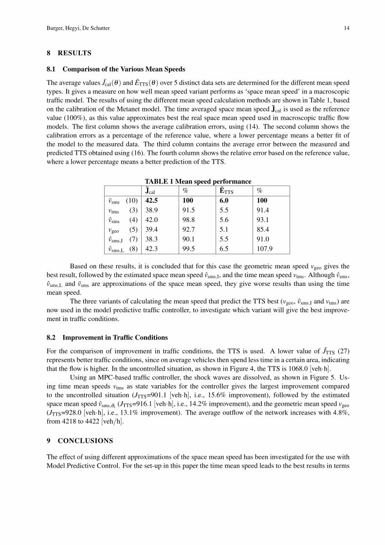
TABLE 1 Mean speed performance
Jcal % ETTS %
vsms (10) 42.5 100 6.0 100
vtms (3) 38.9 91.5 5.5 91.4
vsms (4) 42.0 98.8 5.6 93.1
vgeo (5) 39.4 92.7 5.1 85.4
vsms,I (7) 38.3 90.1 5.5 91.0
vsms,L (8) 42.3 99.5 6.5 107.9
Based on these results, it is concluded that for this case the geometric mean speed vgeo gives the
best result, followed by the estimated space mean speed vsms,I, and the time mean speed vtms. Although vsms,
vsms,L and vsms are approximations of the space mean speed, they give worse results than using the time
mean speed.
The three variants of calculating the mean speed that predict the TTS best (vgeo, vsms,I and vtms) are
now used in the model predictive traffic controller, to investigate which variant will give the best improve-
ment in traffic conditions.
8.2 Improvement in Traffic Conditions
For the comparison of improvement in traffic conditions, the TTS is used. A lower value of JTTS (27)
represents better traffic conditions, since on average vehicles then spend less time in a certain area, indicating
that the flow is higher. In the uncontrolled situation, as shown in Figure 4, the TTS is 1068.0 [veh·h].Using an MPC-based traffic controller, the shock waves are dissolved, as shown in Figure 5. Us-
ing time mean speeds vtms as state variables for the controller gives the largest improvement compared
to the uncontrolled situation (JTTS=901.1 [veh·h], i.e., 15.6% improvement), followed by the estimated
space mean speed vsms,σi(JTTS=916.1 [veh·h], i.e., 14.2% improvement), and the geometric mean speed vgeo
(JTTS=928.0 [veh·h], i.e., 13.1% improvement). The average outflow of the network increases with 4.8%,
from 4218 to 4422 [veh/h].
9 CONCLUSIONS
The effect of using different approximations of the space mean speed has been investigated for the use with
Model Predictive Control. For the set-up in this paper the time mean speed leads to the best results in terms

Burger, Hegyi, De Schutter 15
FIGURE 5 Traffic conditions when using controlled speed limits with time mean speed measurements
of Total Time Spent (TTS).
For the case study that involves a stretch of the A12 freeway in The Netherlands, we have shown
that using an MPC approach, the traffic jam can be resolved and the TTS can be reduced significantly.
Improvements of up to 15.6% compared to the uncontrolled situation are reached. Reducing the shock
waves also has a positive effect on the flow, which is increased by 4.8% using the time mean speed.
For statistically significant conclusions on which mean speed to use and the expected performance
improvements, more calibration and simulation runs are necessary. Based on the current research results it
seems that the differences between using time mean speeds and space mean speeds are small, and in practice,
the time mean speed can be used in model-based traffic control.
ACKNOWLEDGMENTS
This research was supported by the BSIK project “Transition Sustainable Mobility (TRANSUMO)” and the
Transport Research Centre Delft.

Burger, Hegyi, De Schutter 16
REFERENCES
[1] S. Smulders. Control of freeway traffic flow by variable speed signs. Transportation Research Part B,
24(2):111–132, April 1990.
[2] Z. Hou and J.-X. Xu. Freeway traffic density control using iterative learning control approach. In
Intelligent Transportation Systems, volume 2, pages 1081–1086, October 2003. ISBN 0-7803-8125-4.
[3] S. Vukanovic, R. Kates, S. Denaes, and H. Keller. A novel algorithm for optimized, safety-oriented
dynamic speed regulation on highways: INCA. In IEEE Conference on Intelligent Transportation
Systems, pages 260–265. Vienna, Austria, September 2005. ISBN 0-7803-9215-9.
[4] C.-C. Chien, Y. Zhang, and P.A. Ioannou. Traffic density control for automated highway systems.
Automatica, 33:1273–1285, July 1997.
[5] H. Lendz, R. Sollacher, and M. Lang. Nonlinear speed-control for a continuum theory of traffic flow.
In 14th World Congress of IFAC, volume Q, pages 67–72. Beijing, China, 1999.
[6] A. Hegyi, M. Burger, B. De Schutter, J. Hellendoorn, and T.J.J. van den Boom. Towards a practical
application of model predictive control to suppress shock waves on freeways. In Proceedings of the
European Control Conference 2007 (ECC’07), pages 1764–1771. Kos, Greece, July 2007.
[7] A. Hegyi, B. De Schutter, and J. Hellendoorn. Optimal coordination of variable speed limits to suppress
shock waves. IEEE Transactions on Intelligent Transportation Systems, 6(1):102–112, March 2005.
[8] D. Petz and R. Temesi. Means of positive numbers and matrices. SIAM Journal on Matrix Analysis
and Applications, 27(3):712–720, 2005.
[9] C.F. Daganzo. Fundamentals of Transportation and Traffic Operations. Pergamon Press, 3rd edition,
1997. ISBN 0 08 042785 5.
[10] A.D. May. Traffic Flow Fundamentals. Prentice-Hall, Englewood Cliffs, New Jersey, 1990. ISBN
0-13-926072-2.
[11] D.J. Dailey, F.W. Cathey, and S. Pumrin. An algorithm to estimate mean traffic speed using uncali-
brated cameras. Intelligent Transportation Systems, IEEE Transactions on, 1(2):98–107, June 2000.
[12] J.G. Wardrop. Some theoretical aspects of road traffic research. In Institute of Civil Engineers, vol-
ume 1, pages 325–378, 1952.
[13] H. Rakha and W. Zhang. Estimating traffic stream space mean speed and reliability from dual- and
single-loop detectors. Transportation Research Record, 1925:38–47, 2005. ISBN 0309093996.
[14] B.S. Kerner and H. Rehborn. Experimental features and characteristics of traffic jams. Physical Review
E, 53(2):1297–1300, February 1996.
[15] A. Kotsialos, M. Papageorgiou, C. Diakaki, Y. Pavlis, and F. Middelham. Traffic flow modeling of
large-scale motorway networks using the macroscopic modeling tool METANET. IEEE Transactions
on Intelligent Transportation Systems, 3(4):282–292, December 2002.
[16] Quadstone. Paramics v5.1. URL http://www.paramics-online.com/.
[17] P.M. Pardalos and M.G.C. Resende. Handbook of Applied Optimization. Oxford University Press,
Oxford, UK, 2002. ISBN 0-19-512594-0.

Burger, Hegyi, De Schutter 17
[18] The MathWorks. Optimization Toolbox User’s Guide – Version 3.1.1. Natick, Massachusetts, 2007.