suction, hydraulic and strength properties of compacted soils thesis - kizza... · the two major...

Suction, hydraulic and strength properties of compacted

soils

KIZZA RICHARD

School of Civil and Environmental Engineering

2019

Suction, hydraulic and strength properties of compacted

soils

KIZZA RICHARD

School of Civil and Environmental Engineering

A thesis submitted to the Nanyang Technological University

in partial fulfilment of the requirement for the degree of

Doctor of Philosophy

Statement of Originality

I hereby certify that the work embodied in this thesis is the result of original research,

is free of plagiarized materials and has not been submitted for a higher degree to any

other University or Institution

5th December 2019

Kizza Richard

Supervisor Declaration Statement

I have reviewed the content and presentation style of this thesis and declare it free of

plagiarism and of sufficient grammatical clarity to be examined. To the best of my

knowledge, the research and writing are those of the candidate except as

acknowledged by the Author Attribution Statement. I confirm that the investigations

were conducted in accord with the ethic policies and Integrity standards of Nanyang

Technological University and that the research data are presented honestly and

without prejudice

……………………….

Date Assoc. Prof. E.C.Leong

6 Dec 2019 ……………………….

Authorship Attribution Statement

This thesis contains material from two conference papers and two manuscripts submitted to

journals and currently under review where I was either the first or second author. Unless

otherwise referenced, this thesis has been developed with the sole assistance of my supervisor

who contributed ideas on the presentation of the thesis and analysis of the data. My

supervisor has also contributed in way of proof-reading the work herein.

The material from my papers is distributed as follows in the thesis:

Chapter 4 contains material from the papers:

Leong, E.-C., Kizza, R. & Rahardjo, H. Measurement of soil suction using moist filter paper.

E3S Web of Conferences, 2016. EDP Sciences, 10012. Kizza, R & Leong, E.C. Suction measurements using initially dry and initially wet filter

papers. Manuscript submitted to Geotechnical and Testing Journal. Under Review.

Chapter 6 contains material from the papers:

Kizza ,R., Leong, E.C & Rahardjo,H. Matric suction and shear strength of dynamically

compacted soils. In Unsaturated soils: Research and Applications 2014. Taylor and

Francis Group.

Kizza, R & Leong, E.C. Unconfined Strength and Tensile Strength of Compacted soils.

Manuscript submitted to Canadian Geotechnical Journal. Under Review.

Material presented in chapters 5 and 7 is yet to be developed into publishable material.

5th December 2019

Kizza Richard

i

Acknowledgements

I extend my deepest gratitude to my supervisor Associate Professor Leong EngChoon first for

accepting me as student in his research team, secondly for the excellent guidance received

from him during my PhD studies and for his extreme patience with me and the willingness

to address all my knowledge gaps.

My deep appreciation is also extended to Professor Harianto Rahardjo for all the assistance

and encouragement extended to me. Your words of wisdom are always memorable.

I am also grateful to the Geotechnical Engineering Laboratory staff: Mr HengHiang Kim

Vincent, Mr Tan Hiap Guan Eugene, Ms Susie Lim-Ding, and Mr Koh Sun Weng Andy for

all the assistance they extended to me during my experimental work. Special thanks to Mr.

Phua formerly of the Construction workshop for always being ready to help with the

fabrications of the different equipment and apparatus necessary for the studies.

I am equally grateful to the administrative staff of CEE: Ms Ng Soo Ching , Ms Ng Hui Leng

and Ms. Jamillah Bte Sa’adon for always being ready to assist with all manner of

administrative issues.

Special thanks to the many friends just to mention a few: Dr. Huang Wengui (Winston), Mr.

Sam Bulolo, Dr. Martin Wijaya, Dr. Alfrendo Satyanaga, Dr. Zhai Qai, Dr. Zhuoyuan, Mr.

Ashraf Mohammed Assewaff, Mr. Varun Maruvanchery, Mr. Zul, and all treasured friends I

met in Singapore. Thank you for all the assistance in all the forms am sure you know.

To my family back home in Uganda: What can I say? Thank you for the support through the

years. This began many years ago. Thank you indeed.

My PhD studies and subsistence were funded by the Singapore International Graduate Award

(SINGA). The financial assistance from SINGA is gratefully acknowledged.

Last but not least, I extend my greatest gratitude to God the Almighty for bringing me this far

ii

Summary

Although enormous strides have been made in terms of theoretical and experimental

advancements of unsaturated soil mechanics, its application in engineering practice remains

limited. Reasons for limited application include expensive equipment required to measure

unsaturated soil properties, long durations to measure these properties, high level of expertise

required and the lack of simple and accessible tools for the practicing engineer to obtain

unsaturated soil properties especially for routine work.

This background motivated this PhD study with the main objective to evaluate and

investigate simple, economical and accessible techniques of measuring unsaturated soil

properties. Three properties were studied: suction, hydraulic and strength. These properties

were evaluated using dynamically compacted residual soils. Four residual soils obtained from

the two major geological formations of Singapore; Jurong Formation and Bukit Timah

Granite were studied.

For suction measurements, the filter paper method was studied and measurements were

compared with those from a chilled-mirror dewpoint technique. The study investigated the

use of both initially dry and initially wet filter papers in an attempt to reduce equilibration

time and eliminate the need for two calibration curves. The study found that the use of

initially wet filter paper did not reduce equilibration time, equilibration time is dependent on

the mode of contact and that the non-contact filter paper requires much longer time to

equilibrate. For low suctions, the non-contact filter paper may not reach equilibrium within

the common durations used in literature of 7, 15, 21 or 28 days. Although there is a tendency

for an initially wet filter paper used in the non-contact mode to approach the matric suction

calibration curve, it may not reach equilibrium at the matric suction calibration curve within a

practical time frame. The contact filter paper which measures matric suction can reliably

iii

measure suctions both in the low and high range while the non-contact is best suited for

suctions in the high range preferable above 1000 kPa. The hysteretic behavior was

investigated by comparing suction measurements from initially dry and initially wet filter

papers. A hysteresis within the range 3-5% was observed. Using this hysteresis, existing

calibration curves can be modified to read suction from initially wet filter papers. Generally,

an initially dry filter paper is preferable to an initially wet filter paper for both contact modes

because an initially dry filter paper requires a less strict protocol. Finally, the study compared

variation in filter papers before and after use and found that the variations were minor to

warrant use of sacrificial filter papers as recommended in ASTM D5298-16.

Hydraulic properties of compacted soils were studied using a mini-disk infiltrometer and the

conventional flexible wall permeameter were compared. A good agreement was found

between the two. Because, the interpretation of the mini-disk infiltrometer requires prior

knowledge of van Genutchen SWCC equation parameters, different approaches of obtaining

these parameters were studied. It was found that all the approaches yield saturated

permeabilities within two orders from the saturated permeability measured from the flexible

wall permeameter. This being within acceptable error margin means that the mini-disk

infiltrometer can be applied reliably to measure near saturated permeabilities hence reducing

testing time for field permeability measurements.

Lastly, using conventional strength tests like the Brazilian tensile strength test, unconfined

compression test, unconsolidated undrained shear strength test and consolidated undrained

test, strength of the compacted soils were investigated. Observations suggest that shear

strength parameters of unsaturated soils may be estimated from an initial suction

measurement and the saturated shear strength parameters. Bounds of shear strength using

Bishop’s factor was evaluated and it seems possible to obtain a lower bound that is

appropriate for engineering practice.

iv

Table of contents

Acknowledgements ............................................................................................................................ i

Summary ........................................................................................................................................... ii

Table of contents .............................................................................................................................. iv

List of Tables ................................................................................................................................... ix

List of Figures ................................................................................................................................... x

List of symbols/Abbreviations ........................................................................................................ xiv

Chapter 1. Introduction ................................................................................................................ 1

1.1 Background to the study........................................................................................................... 1

1.2 Objectives and Scope ............................................................................................................... 2

1.3 Thesis Outline and description of the report. ............................................................................ 4

Chapter 2. Literature Review ....................................................................................................... 6

2.1 Introduction ............................................................................................................................. 6

2.2 Unsaturated soils and their prevalence ...................................................................................... 6

2.3 Stress state variables for unsaturated soils ................................................................................ 8

2.3.1 Single effective stress approach. ........................................................................................ 9

2.3.2 Independent stress state variable approach ....................................................................... 10

2.3.3 Alternative /Modified stress variables approach ............................................................... 11

2.4 Soil Suction ........................................................................................................................... 14

2.4.1 Definitions of suction ...................................................................................................... 14

2.4.2 Matric suction ................................................................................................................. 14

2.4.3 Total suction ................................................................................................................... 16

2.4.4 Suction control and measurements................................................................................... 17

2.4.4.1Techniques for controlling suction ............................................................................. 18

2.4.4.2 Suction measurement techniques .............................................................................. 23

2.5 Soil-water characteristic curves .............................................................................................. 36

2.5.1 Factors affecting the SWCC ................................................................................................ 39

2.5.1.1 Influence of soil type ................................................................................................ 39

2.5.1.2 Influence of soil structure ......................................................................................... 41

2.5.1.3 Effect of initial density the SWCC ............................................................................ 42

2.5.1.4 Effect of stress history and methods of sample preparation ....................................... 42

2.5.2 Equations for soil-water characteristic curves .................................................................. 45

2.5.2.1 Gardner (1958) ......................................................................................................... 46

2.5.2.2 Brooks and Corey (1964) .......................................................................................... 46

v

2.5.2.3 van Genuchten (1980) ............................................................................................. 47

2.5.2.4 Fredlund and Xing (1994) ......................................................................................... 47

2.6 Permeability .......................................................................................................................... 49

2.6.1 Saturated permeability ..................................................................................................... 49

2.6.2Unsaturated permeability.................................................................................................. 52

2.6.2.1 Relationship between unsaturated permeability and volume-mass relations of soils ... 52

2.6.2.2 Permeability functions .............................................................................................. 53

2.6.3 Laboratory measurement of permeability ......................................................................... 58

2.6.3.1 Saturated permeability .............................................................................................. 58

2.6.3.2 Unsaturated permeability .......................................................................................... 60

2.6.4 Field measurements of permeability in the vadose zone ................................................... 61

2.6.4.1 Constant head well permeameter .............................................................................. 61

2.6.4.2 Ring infiltrometers ................................................................................................... 64

2.6.4.3 Tension or disk infiltrometers ................................................................................... 66

2.7 Shear strength of unsaturated soils ......................................................................................... 70

2.7.1 Shear strength equations of unsaturated soils ................................................................... 71

2.7.1.1 Single stress state variable approach ......................................................................... 71

2.7.1.2 The independent stress state variable approach ......................................................... 75

2.7.1.3 Shear strength equations formulated from alternative stress variables ........................ 79

2.7 Shear strength testing for unsaturated soils ............................................................................. 81

2.8 Concluding remarks ............................................................................................................... 83

Chapter 3. Research Programme ................................................................................................ 86

3.1 Introduction ........................................................................................................................... 86

3.2 Soils and basic properties .................................................................................................... 86

3.3 Compaction behavior and preparation of test specimens ......................................................... 90

3.3.1 Justification for use of compacted materials..................................................................... 90

3.3.2 Preparation of test specimens .......................................................................................... 92

3.3.3 Nomenclature of the test specimens ................................................................................. 98

3.4 Suction measurements.......................................................................................................... 100

3.4.1 Filter paper technique .................................................................................................... 100

3.4.1.1 Initially dry filter papers ..................................................................................... 100

3.4.1.2 Initially wet filter papers ......................................................................................... 101

3.4.2 Chilled mirror dew-point technique ............................................................................... 106

3.5 Soil-water characteristics curves .......................................................................................... 107

3.5.1 Pressure plate tests ........................................................................................................ 108

3.5.2 Chilled mirror dew-point test ......................................................................................... 109

vi

3.6 Hydraulic properties of compacted soils .............................................................................. 110

3.6.1 Infiltration test using a mini-disk infiltrometer ............................................................... 110

3.6.2 Falling head flexible-wall permeameter ........................................................................ 112

3.7 Strength tests ....................................................................................................................... 114

3.7.1 Unconfined Compression test ........................................................................................ 115

3.7.2 Brazilian Tensile Strength test ...................................................................................... 116

3.7.3 Unconsolidated Undrained test ...................................................................................... 118

3.7.4 Consolidated Undrained test for saturated soils .............................................................. 119

Chapter 4. Soil Suction measurements and Soil-Water Characteristic Curves ........................... 121

4.1 Introduction ......................................................................................................................... 121

4.2 Suction measurements using the filter paper method ............................................................ 121

4.2.1 Equilibration time for filter papers ................................................................................. 122

4.2.2 Initial moisture condition of filter paper........................................................................ 126

4.2.3 Hysteresis ..................................................................................................................... 133

4.2.4 Suction measurements ................................................................................................... 134

4.2.5 Variability of filter papers ............................................................................................. 141

4.2.6 Summary ..................................................................................................................... 142

4.3 Soil-water characteristic curves of compacted soils .............................................................. 143

4.3.1 SWCC-w ...................................................................................................................... 146

4.3.2 SWCC-S ....................................................................................................................... 152

4.3.2.1 Effect of compaction water content on SWCC-S .................................................... 154

4.3.2.2 Effect of compaction effort on SWCC-S ................................................................. 155

4.3.3 Comparison of SWCCs with previous studies ................................................................ 160

4.4 Comparison of suctions from filter paper method and SWCC ............................................... 163

4.5 Concluding remarks ............................................................................................................. 164

Chapter 5. Hydraulic properties of compacted soils.................................................................. 167

5.1 Introduction ......................................................................................................................... 167

5.2 Soils studied ........................................................................................................................ 168

5.3 Saturated Permeability ......................................................................................................... 171

5.3.1 Variation of ks with compaction water content ............................................................... 172

5.3.2 Variation of ks with void ratio ....................................................................................... 172

5.4 Infiltration tests using a mini-disk infiltrometer. ................................................................... 174

5.4.1 Infiltration rates............................................................................................................. 174

5.4.1.1 Effect of suction head on infiltration ....................................................................... 176

5.4.1.2 Effect of compaction water content on infiltration ................................................... 176

5.4.1.3 Effect of compaction effort on infiltration ............................................................... 182

vii

5.4.2 Estimation of near saturated permeability using infiltration measurements ..................... 184

5.4.2.1 Case studies for parameter A2 ................................................................................. 184

5.4.2.2Soil water characteristic curves (SWCC) ................................................................. 186

5.4.2.3 Comparison of permeabilities obtained from the falling head permeability test and

mini-disk infiltrometer ....................................................................................................... 188

5.5 Statistical permeability model .............................................................................................. 191


Chapter 6. Unconfined Compressive Strength and Tensile Strength of compacted soils ............ 196

6.1 Introduction ......................................................................................................................... 196

6.2 Test Series 1 - As-compacted soil specimens ........................................................................ 197

6.2.1 Stress- strain plots for UCS test ..................................................................................... 197

6.2.2 Unconfined compressive strength and Brazilian tensile strength .................................... 204

6.3 Test Series 2 -Pre-dried specimens compacted wet of optimum ........................................... 209

6.3.1 Stress- strain plots for UCS test ..................................................................................... 211

6.4 Tensile strength models ....................................................................................................... 217

6.4.1 Lu etal. (2009) tensile strength model ........................................................................... 217

6.4.2 Yin and Vanapalli (2018) tensile strength model ........................................................... 222

6.4.3 Summary ...................................................................................................................... 231


Chapter 7. Constant water content shear strength tests on compacted soils ............................... 234

7.1 Introduction ......................................................................................................................... 234

7.2 Unconfined compression and unconsolidated undrained tests ............................................... 235

7.2.1 Stress-strain behavior .................................................................................................... 235

7.2.1.1 Effect of net confining pressure .............................................................................. 235

7.2.1.2 Effect of compaction water content ........................................................................ 238

7.2.1.3 Effect of compaction effort ................................................................................... 240

7.2.2 Peak strength ................................................................................................................. 242

7.3 Saturated shear strength parameters ...................................................................................... 245

7.4 Proposed interpretation of the CW test ................................................................................. 252


8. Conclusion and Recommendations ............................................................................................ 263

8.1 Conclusions ......................................................................................................................... 263

8.1.1 Suction measurements ................................................................................................... 263

8.1.2 Permeability measurements ........................................................................................... 264

8.1.3 Unconfined compressive strength and tensile strength .................................................. 265

8.1.4 Constant water content tests .......................................................................................... 266

viii

8.2Recommendations................................................................................................................. 266

References..................................................................................................................................... 269

APPENDICES .............................................................................................................................. 281

Appendix A-Suction and SWCC data ............................................................................................ 282

Appendix B-Hydraulic properties .................................................................................................. 307

Appendix C- UC and BTS data ...................................................................................................... 345

Appendix D-UC and UU data ........................................................................................................ 352

ix

List of Tables

Table 2.1: Suction control and Suction measurement techniques (Ridley and Wray, 1996; Blatz et al,

2008; Bulut and Leong, 2008; Masrouri et al, 2008; Vanapalli et.al, 2008)....................................... 33

Table 2.2: Calibration curves for Whatman No.42 and Schleicher & Schuell No.589 filter papers .... 34

Table 2.3 Relationships of unsaturated permeability with void ratio and degree of saturation ........... 54

Table 2.4 VG model calibration parameters for 12 soils (Carsel and Parrish, 1988) .......................... 70

Table 2.5: A comparison of selected shear strength equations to a generalised form (adopted from

Leong 2019) .................................................................................................................................... 79

Table 3.1: Basic properties of soils studied ...................................................................................... 87

Table 3.2: Parameters defining the GSD envelopes for BT and JF formations (from Rahardjo et al.,

2012) ............................................................................................................................................... 90

Table 3.3: Compaction properties of soils studied ............................................................................ 93

Table 3.4 Comparison between the ASTM and thesis procedures of compaction .............................. 95

Table 3.5: A guide to the nomenclature adopted for the different test specimens .............................. 99

Table 4.1: Average properties for BT1 specimens measured for SWCC ......................................... 144

Table 4.2: Average properties for BT2 specimens measured for SWCC ......................................... 145

Table 4.3: Average properties of JF1 specimens measured for SWCC ............................................ 145

Table 4.4: Average properties for JF2 specimens measured for SWCC .......................................... 146

Table 4.5: SWCC fitting parameters for Singapore residual soils (after Agus et.al 2001) ................ 161

Table 5.1: Properties of BT1 soil specimens whose hydraulic properties were studied .................... 169

Table 5.2: Properties of BT2 soil specimens whose hydraulic properties were studied .................... 170

Table 5.3: Properties of JF2 soil specimens whose hydraulic properties were studied ..................... 170

Table 5.4: Summary of C2coefficientsfor the different soil specimens at the different suction heads 185

Table 6.1: Properties of BT1 test specimens ................................................................................... 200

Table 6.2: Properties of BT2 test specimens ................................................................................... 200

Table 6.3: Properties of JF1 test specimens .................................................................................... 201

Table 6.4: Properties of JF2 test specimens .................................................................................... 201

Table 6.5: Relationship of suction with compaction water content.................................................. 209

Table 6.6: Average properties of sample sets A to I in Test series 2................................................ 211

Table 6.7: Shear strength and SWCC equations parameters for sample sets A-I ............................. 220

Table 6.8: Summary of RMSE for Lu et.al (2009) tensile strength model ....................................... 225

Table 6.9: Parameters for Yin and Vanapalli (2018) tensile strength model for Cases 1 to 4 ........... 230

Table 7.1: Variation of friction angles for the different soils........................................................... 250

x

List of Figures

Figure 2.1: Interaction between unsaturated zone and the hydrological cycle (from Lu and Likos,

2004) ................................................................................................................................................. 7

Figure 2.2: Illustration of flux processes in the unsaturated (vadose) zone (from Fredlund and

Rahardjo, 1993) ................................................................................................................................. 7

Figure 2.3: Schematic illustration of water adsorption on clay particle surafces (from Baker and

Frydman, 2009) ............................................................................................................................... 16

Figure 2.4: Illustration of the axis-translation technique ................................................................... 19

Figure 2.5: Vapor equilibrium technique (from Leong and Rahardjo, 2002) ..................................... 20

Figure 2.6: Application of the osmotic technique to impose suction on a soil sample (from Cui and

Delage, 1996) .................................................................................................................................. 22

Figure 2.7: High Capacity tensiometer (after Ridley et.al, 2003) ...................................................... 24

Figure 2.8: A schematic of the chilled-mirror dewpoint hygrometer (after Leong et al., 2003). ......... 26

Figure 2.9: Calibration data for the filter papers from different researchers (from Rahardjo and Leong,

2006) ............................................................................................................................................... 35

Figure 2.10: Drying SWCC showing the variables and the different zones(Fredlund, 2006) ............. 36

Figure 2.11: Typical SWCC for a silt soil (from Fredlund et al, 2012) .............................................. 38

Figure 2.12: Influence of soil texture on SWCC (Vanapalli, 1994; Barbour, 1998) ........................... 39

Figure 2.13: SWCCs for compacted soil at different initial moulding water contents (from Vanapalli,

1994) ............................................................................................................................................... 41

Figure 2.14: Effect of initial density on SWCC of a soil: a) pre-consolidated Regina clay (Fredlund,

1967), and b) compacted clayey silty sand (Salager et al., 2010) ...................................................... 44

Figure 2.15: Effect of stress history and methods of specimen preparation on the SWCC (Fredlund,

2002) ............................................................................................................................................... 45

Figure 2.16: Calculation of the permeability function from the SWCC (from Marshall, 1958; Kunze et

al, 1968 ) ......................................................................................................................................... 58

Figure 2.17: Schematic representation of a) the constant head well permeameter(Reynolds and Elrick,

2002), and b) the simulation domain(Hayashi and Quinton, 2004) ................................................... 63

Figure 2.18: Cross sections of a) Single ring infiltrometer, b) Double (concentric) ring

infiltromer(Reynolds et al., 2002b) .................................................................................................. 64

Figure 2.19: Extended Mohr-Coulomb failure envelope (from Fredlund and Rahardjo, 1993) .......... 76

Figure 3.1: Grain size distributions for the studied soils ................................................................... 88

Figure 3.2: Grain size distributions: a) BT and b) JF soils in comparison with the upper and lower

bound GSDs and typical GSD.......................................................................................................... 89

Figure 3.3: Moisture-density relationships: a) Typical compaction curve, b) Effect of compaction on

soil structure (Lambe, 1958) ............................................................................................................ 91

Figure 3.4: Moisture-density relationships for the soils studied at both standard and modified Proctor

energies ........................................................................................................................................... 94

Figure 3.5: Compaction set-up to prepare soil specimens in the PVC mould..................................... 97

Figure 3.6: Typical compaction specimens, left specimen obtained using the PVC mould and the right

specimen using the ASTM standard compaction mould ................................................................... 98

Figure 3.7: Preparation of soil specimen for suction measurement using filter paper technique ....... 104

Figure 3.8: Filter paper handling post equilibration. ....................................................................... 105

Figure 3.9: Mounting a test specimen with the chilled mirror hygrometer ...................................... 107

xi

Figure 3.10: Pressure plate system ................................................................................................. 108

Figure 3.11: Infiltration test using a mini-disk infiltrometer ........................................................... 111

Figure 3.12: Flexible wall permeameter set up ............................................................................... 112

Figure 3.13: Compacted sample prepared for sawing to obtain BTS test specimens ........................ 117

Figure 4.1: Moisture-density relationships for the study materials used in suction measurements ... 123

Figure 4.2: Effect of equilibrium time on filter paper water content for standard Proctor compacted

BT1 soils- Standard mold and Method 1 ........................................................................................ 127

Figure 4.3: Effect of equilibrium time on filter paper water content for modified Proctor compacted

BT1 soils- Standard mold and Method 1 ........................................................................................ 128

Figure 4.4: Effect of equilibrium time on filter paper water content for standard Proctor compacted

JF2 soils- Standard mold and Method 1 ......................................................................................... 129

Figure 4.5: Effect of equilibrium time on filter paper water content for modified Proctor compacted

JF2 soils- Standard mold and Method 1 ......................................................................................... 130

Figure 4.6: Drying pattern of 12 initially wet filter papers .............................................................. 131

Figure 4.7: Comparison of contact and non-contact initially dry filter papers ................................. 132

Figure 4.8:Comparison of contact and non-contact initially wet filter papers .................................. 133

Figure 4.9: Hysteresis between initially dry and initially wet filter papers in contact and non-contact

modes............................................................................................................................................ 136

Figure 4.10: Suction calibration curves for initially dry and initially wet filter paper in non contact

mode ............................................................................................................................................. 137

Figure 4.11: Comparison of initially dry non-contact filter paper measurement of suction with other

researchers .................................................................................................................................... 138

Figure 4.12: Comparison of suction measurements by initially dry non-contact filter paper and chilled

mirror dewpoint technique ............................................................................................................. 140

Figure 4.13: Weight distribution of dried filter papers before and after use ..................................... 142

Figure 4.14: SWCC-w for samples compacted in the standard mould ............................................. 148

Figure 4.15: SWCC-w for specimens compacted in the plastic mould ............................................ 149

Figure 4.16: SWCC-w plotted in terms of normalised gravimetric water contents for soil specimens

compacted in the standard mould ................................................................................................... 151

Figure 4.17: Typical shrinkage curves............................................................................................ 153

Figure 4.18:SWCC-S for JF2 soil specimens compacted at standard and modified Proctor efforts in

the plastic mould ........................................................................................................................... 156

Figure 4.19: SWCC-S for JF2 soil specimens compacted at standard and modified Proctor efforts in

the standard mould ........................................................................................................................ 157

Figure 4.20: SWCC-S for BT1 soil specimens compacted dry and wet of optimum in the plastic

mould at standard and modified Proctor efforts .............................................................................. 158

Figure 4.21: SWCC-S for BT1 soil specimens compacted dry and wet of optimum in the standard

mould at standard and modified Proctor efforts .............................................................................. 159

Figure 4.22: Variation of AEV with dry density ............................................................................. 160

Figure 4.23: Comparison of SWCC data with SWCC envelopes suggested by Agus et al. (2001) ... 162

Figure 4.24: Comparison of suctions measured using filter paper technique and suctions estimated

from the SWCC ............................................................................................................................. 163

Figure 5.1: Moisture-density relationships for the soil studied together with the specific test points 168

Figure 5.2: Variation of ks with compaction water content ............................................................. 173

Figure 5.3: Variation of ks with void ratio ..................................................................................... 174

xii

Figure 5.4: Cumulative infiltration vs square root time at three suction heads for selected BT2 soil

specimens ...................................................................................................................................... 177

Figure 5.5: Cumulative infiltration vs square root time at three suction heads for selected JF2 soil

specimens ...................................................................................................................................... 178

Figure 5.6: Comparison of infiltration rates for different compaction water contents at given suction

heads for BT1 soils compacted at standard and modified Proctor efforts ........................................ 180

Figure 5.7: Comparison of infiltration rates for different compaction water contents at given suction

heads for JF2 soils compacted at standard and modified Proctor efforts. ......................................... 181

Figure 5.8: Comparison of infiltration rates for different water compaction water contents at given

suction heads for both standard and modified Proctor energies for BT1 soil specimens .................. 183

Figure 5.9: Typical SWCC plots for the Cases 1, 2 and 3 ............................................................... 187

Figure 5.10: Comparison of permeabilities from FWP and the different study case ........................ 189

Figure 5.11: Comparison of saturated and estimated permeabilities for different cases for BT1 soil 190

Figure 5.12: Comparison of saturated and estimated permeabilities for different cases for BT2 soil 190

Figure 5.13: Comparison of saturated and estimated permeabilities for different cases for JF2 soil . 191

Figure 5.14: Variation of kr with suction for soil specimens compacted at standard Proctor effort .. 193

Figure 5.15: Variation of kr with suction for soil specimens compacted at modified Proctor effort .. 194

Figure 6.1: BT1 Test series 1 specimens ........................................................................................ 198

Figure 6.2: JF Test series 1specimens ............................................................................................ 199

Figure 6.3: Stress-strain plots from UCS test for BT1 and JF2 soil specimens compacted at both

standard and modified Proctor efforts ............................................................................................ 202

Figure 6.4: Stress-strain plots from UCS test for both standard and modified Proctor compacted soils

...................................................................................................................................................... 203

Figure 6.5: UCS and BTS with compaction water content-Test series 1 ......................................... 205

Figure 6.6: Variability of the BTS for disk specimens taken from different compaction layers with dry

density-Test series 1 ...................................................................................................................... 207

Figure 6.7: Variation of suction with compaction water content ..................................................... 208

Figure 6.8: BT1 test series 2 specimens ......................................................................................... 210

Figure 6.9: BT2 test series 2 specimens ......................................................................................... 210

Figure 6.10: JF2 test series 2 specimens ......................................................................................... 211

Figure 6.11: Stress-strain plots for sample sets A, B and C-Test series ........................................... 214

Figure 6.12: Variation of UCS and BTS with degree of saturation and SWCC for sample sets A to C-

Test series 2 .................................................................................................................................. 215

Figure 6.13: Variation of qu/σtwith degree of saturation for sample sets A to I- Test series 2 .......... 216

Figure 6.14: Determination of t from UCS and BTS .................................................................... 218

Figure 6.15: Variation with degree of saturation for sample sets A to G - Test series 2 ................... 221

Figure 6.16: Evaluation of Lu et.al (2009) tensile strength model ................................................... 224

Figure 6.17: Evaluation of Yin and Vanapalli (2018) tensile strength model .................................. 229

Figure 7.1: Deviator stress versus axial strain plots for UC and UU tests ........................................ 237

Figure 7.2: Effect of compaction water content on the stress-strain behaviour of compacted test

specimens ...................................................................................................................................... 239

Figure 7.3: Influence of compaction effort on the stress-strain plots ............................................... 241

Figure 7.4:Peak strength variation with net confining pressure , compaction water content and

compaction efforts ......................................................................................................................... 243

Figure 7.5: Typical Mohr circle plots for the UC and UU tests ....................................................... 244

xiii

Figure 7.6: Typical stress-strain plots for the CU multi-stage test and the derived Mohr-Coulomb

envelope ........................................................................................................................................ 245

Figure 7.7:Variation of friction angle with dry density and compaction water content .................... 246

Figure 7.8: Variation of effective cohesion with dry density and compaction water content ............ 247

Figure 7.9: Errors in determining shear strength parameters of compacted soils ............................. 249

Figure 7.10: Effective cohesion using an average friction angle for each compaction effort ............ 251

Figure 7.11: Typical plots showing UU Mohr circles fitted with tangent lines at the respective

effective friction angles ................................................................................................................. 253

Figure 7.12: Variation of total cohesion with net confining pressure for BT1 soils compacted at

standard and modified Proctor efforts ............................................................................................ 254

Figure 7.13: A single line for Mohr circles of specimens compacted dry of optimum ..................... 256

Figure 7.14: Plots of tanφb/tanφ’ versus degree of satration for the as-compacted soil specimens.... 257

Figure 7.15: Plots of tanφb/tanφ’ versus degree of saturation for the as-compacted and dried soil

specimens ...................................................................................................................................... 259

Figure 7.16: Variation of χ with suction ratio ................................................................................. 260

xiv

List of symbols/Abbreviations

𝐴 Cross sectional area of a soil specimen

a Fredlund and Xing (1994) SWCC model fitting parameter

𝛼 van Genuchten (1980) model fitting parameter

AEV Air-entry value of soil

𝑐′ Effective soil cohesion

CW Constant water content test

𝐸 Total energy

e void ratio

emin Minimum void ratio

e0 Initial void ratio

𝑔 Gravitational acceleration

Gs Specific gravity

𝛾𝑤 Specific weight of water

HAE High Air Entry

HCT High Capacity Tensiometer

h𝑤 Hydraulic head or total head

h1 Head of water at t1

xv

h2 Head of water at t2

Δh𝑤 Hydraulic head difference

𝑀𝑤 Mass of water a selected point

m A fitting parameter related to residual water content

𝜇 Viscosity of a fluid

𝑛 van Genuchten (1980) model fitting parameter

𝑝 Pressure

𝛩 Normalized volumetric water content

𝜃 volumetric water content

𝜃s Saturated volumetric

𝑅𝑀𝑆𝐸 Root mean square error

𝑅 Universal gas constant

𝑟 Distance from center of circular tube from concentric cylindrical surface

𝜌𝑤 Density of water

𝜌 Pore radius

𝑆 Degree of saturation

Se Effective degree of saturation

𝑆𝑟 Residual degree of saturation

xvi

SWCC Soil Water Characteristic Curve

SWCC-S Soil Water Characteristic curve based on degree of saturation

SWCC-w Soil Water Characteristic curve based on gravimetric water content

SWCC-θ Soil Water Characteristic curve based on volumetric water content

𝑇 Absolute temperature

𝑇𝑠 Surface tension

𝑡 Time

𝜏 Shear strength

𝑢𝑎 Pore-air pressure

𝑢𝑤 Pore-water pressure

𝑢𝑎−𝑢𝑤 Matric suction

ū𝜐 Partial pressure of pore-water vapor

ū𝜐0 Saturation pressure of water vapor over a flat surface of pure water at the same

temperature

w gravimetric water content

χ Bishop’s effective stress parameter

d Dry density

𝜓 Soil suction

xvii

𝜓r Suction corresponding to residual water content

σ Total normal stress

σ’ Effective normal stress

σ-ua Net normal stress

1

Chapter 1. Introduction

1.1 Background to the study

Although geotechnical engineering practice has registered enormous success over the decades

with the application of saturated soil mechanics, it is increasingly becoming clear that

unsaturated soil mechanics can explain several phenomena better such as rain-induced slope

failures. Commonly, these slope instabilities occur during rainy seasons of the year and in

unsaturated materials. These landslides result in loss of lives as well as destruction of

property. It has been noted by several researchers (e.g. Toll et al. 1999, Rahardjo et al.,2009,

2013) that understanding the cause as well as design of remedial systems require sound

knowledge of unsaturated soil mechanics.

Secondly, major geotechnical structures like dams, foundations are often located in the

unsaturated zone which means that they are influenced by the negative pore-water pressures

(Tarantino and El Mountassir, 2013). Therefore it is important to consider ground-

atmosphere interactions that will influence their performance throughout their design life.

More care is needed when these geotechnical structures are built in soils susceptible to

collapse and swelling on wetting to avoid future remedial costs that may arise if ignored.

The adoption of unsaturated soil mechanics principles in the design of geotechnical structures

may also avoid the problem of over design often encountered when full saturation of soils is

assumed in designs (Tarantino and El Mountassir (2013). Despite these glaring demands for

unsaturated soil mechanics, unsaturated soil mechanics largely remains in research

institutions with little application in practice. The low application of unsaturated soil

mechanics is largely due to excessive costs and time required to determine unsaturated soil

properties such as soil suction, permeability and shear strength (Fredlund, 2000; Tarantino

2

and El Mountassir, 2013; Vanapalli, 1995; Oh, 2012).With these obstacles, the practical

application of unsaturated soil mechanics principles remains low especially in developing

economies. Ironically, these principles are most needed in the developing world which lies in

the tropics where unsaturated soils are often encountered.

To incorporate unsaturated soil mechanics into routine engineering practice will require more

accessible tests to measure the soil properties. In some cases, this entails improvements to the

existing experimental protocols. In addition, there is a need to connect unsaturated soil

mechanics empirically or analytically with the experiences already gained from saturated soil

mechanics.

Therefore, this research attempts to study the performance and reliability of simple,

economical experimental techniques and procedures with the major aim of extending

unsaturated soil mechanics to engineering practice.

1.2 Objectives and Scope

The main objective of this study is to investigate and evaluate simple, affordable and yet

reliable tests to determine unsaturated soil properties. The study is motivated by the need to

make unsaturated soil mechanics more accessible to practicing engineers especially those in

developing countries. The study focuses on:

Suction measurements:

Although the filter paper and chilled-mirror dewpoint techniques are already in use as suction

measurement techniques, researchers have not agreed on a number of issues regarding their

use. For the filter paper technique, a number of studies have been done and the method has

been standardized (ASTM D5298-16). However, its acceptance by researchers and

practitioners has remained low largely because of questions on reliability. Using dynamically

3

compacted soils, several aspects of the filter paper technique are studied. The main factors

investigated are equilibration time, hysteresis of the filter paper, applicable calibration curve,

and inherent variability of the filter papers. Initially wet filter paper was explored with the

aim of establishing any advantages over the conventional initially dry filter paper. The

chilled-mirror dewpoint technique was used to benchmark against filter paper measurements

for high suctions. Many filter paper tests were performed. It is envisaged that the experience

and discussions greatly improve the understanding of this valuable yet very accessible

technique.

Hydraulic properties:

Permeability is an important parameter in modelling water flow through soils and is needed

in several geotechnical engineering problems such as rain-induced landslides, seepage

through dams, and design of waste management systems. However, most of the existing

techniques for measuring permeability are laborious, time consuming and may not represent

actual field conditions. This study has therefore explored the use of the mini-disk

infiltrometer in the estimation of near-saturated permeabilities of soils. The disk infiltrometer

has been reported as inexpensive, robust and gives fast measurements of permeability.

Despite these attributes, the disk infiltrometer has not been widely adopted by the

geotechnical engineering community. Most of the existing studies on the disk infiltrometer

have been done by soil scientists and hydrologists. In this study, permeability measurements

using a disk infiltrometer were done on compacted soils and compared with measurements

from the flexible wall permeameter. The findings and discussions are presented in the thesis.

4

Shear strength measurements:

Shear strength of soil is very crucial in the design of any geotechnical structure. It is also

necessary in back analyses of failed geotechnical structures and for designing remedial

measures. However measuring unsaturated soil shear strength is not only laborious but takes

a long time and requires expensive equipment and high level of expertise to interpret the test

results.

Therefore the study also investigates the possibility of determining shear strength of

unsaturated soils using conventional soil test equipment and constant water content (CW)

tests. In the thesis, unconfined compressive strength tests, unconsolidated undrained tests as

well as the consolidated undrained test for saturated soils are also examined to interpret a

constant water content shear strength test. Shear strength and tensile strength of dried and as-

compacted soil specimens were examined to investigate the effects of soil structure, soil

suction and void ratio.

1.3 Thesis Outline and description of the report.

This report consists of eight chapters and appendices:

Chapter One outlines the background of the study, its significance, objectives and scope.

Chapter Two reviews the literature relevant to the study. The literature review highlights the

current state of knowledge in terms of theoretical advancements as well as the experimental

techniques relevant to the thesis. The key debates and points of contention are highlighted

and finally, the gaps the study aims to fill are pointed out.

In Chapter Three, the soil materials and the test specimen preparation are presented. The

experimental work including the tests, equipment and apparatus used are also presented. The

5

test procedures followed have been noted and where deviations from the standards have been

made, this too has been highlighted.

Chapter Four presents the results and discussion on suction measurements and soil-water

characteristic curves of the test specimens.

Chapter Five presents results and discussion of the hydraulic properties of compacted soils.

Both infiltration studies and measurements of saturated permeabilities in a flexible wall

permeameter are presented.

Chapter Six presents results and discussion of the unconfined compressive strength and

tensile strength of compacted soils.

Chapter Seven presents the results and interpretation of constant water content tests done

using the unconfined compressive strength tests, unconsolidated undrained strength tests and

the consolidated undrained tests on saturated soil specimens

Chapter Eight presents the conclusions of this study as well as the recommendations for

further work.

Appendices

Finally appendices containing data either secondary to the discussions in the thesis or primary

data in excess of what could be presented in the main thesis.

6

Chapter 2. Literature Review

2.1 Introduction

This chapter presents a review of the literature related to the different aspects of the study.

The chapter covers the basic concepts related to unsaturated soil mechanics, water retention

behavior, soil suction measurements and control, hydraulic behavior and strength of

unsaturated soils. The review includes both the governing theories and experimental

techniques commonly used in measuring the various properties of unsaturated soils. The

chapter concludes by justifying the need for the present study

2.2 Unsaturated soils and their prevalence

While the pore space of saturated soils is completely filled with a liquid (typically water), that

of unsaturated soils is partly filled with water and air. The inclusion of air in the pores makes

unsaturated soils a multi-phase porous system. The behavior of these soils is controlled by the

mutual interaction between the two phases (air and water) with the solid component

(Fredlund and Rahardjo, 1993; Laloui, 2013).The mechanisms of interaction in such a multi-

phase system introduce several complexities in terms of material behavior, testing techniques

and numerical modeling (El Mountassir, 2011).

Unsaturated soils are prevalent especially in the tropical region of the world. In these areas,

the near ground surface is usually unsaturated, i.e. has negative pore-water pressures, due to

climatic conditions,. The depth of the unsaturated zone varies according to the local climatic

conditions, ranging from several metres deep in the arid regions to just a few metres in the

temperate zone. Figure 2.1 shows a simplified hydrological cycle in nature illustrating the

complex interactions between climate, atmosphere and the ground. It is shown how the

ground loses water to the atmosphere through evaporation and evapotranspiration. These

7

processes (evaporation and evapotranspiration) result into an upward flux for soil moisture

causing drying, desaturation and desiccation cracks in the soils. On the other hand, the soil is

recharged during a precipitation, Hence, a downward flux of water which results into an

increase in the soil’s degree of saturation and increase in pore-water pressure.

Figure 2.1: Interaction between unsaturated zone and the hydrological cycle (from Lu and

Likos, 2004)

Figure 2.2: Illustration of flux processes in the unsaturated (vadose) zone (from Fredlund and

Rahardjo, 1993)

8

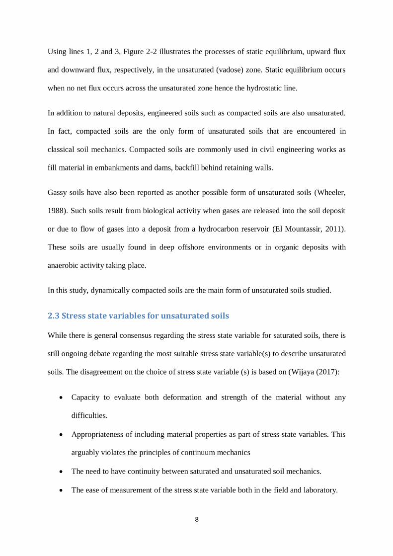
Using lines 1, 2 and 3, Figure 2-2 illustrates the processes of static equilibrium, upward flux

and downward flux, respectively, in the unsaturated (vadose) zone. Static equilibrium occurs

when no net flux occurs across the unsaturated zone hence the hydrostatic line.

In addition to natural deposits, engineered soils such as compacted soils are also unsaturated.

In fact, compacted soils are the only form of unsaturated soils that are encountered in

classical soil mechanics. Compacted soils are commonly used in civil engineering works as

fill material in embankments and dams, backfill behind retaining walls.

Gassy soils have also been reported as another possible form of unsaturated soils (Wheeler,

1988). Such soils result from biological activity when gases are released into the soil deposit

or due to flow of gases into a deposit from a hydrocarbon reservoir (El Mountassir, 2011).

These soils are usually found in deep offshore environments or in organic deposits with

anaerobic activity taking place.

In this study, dynamically compacted soils are the main form of unsaturated soils studied.

2.3 Stress state variables for unsaturated soils

While there is general consensus regarding the stress state variable for saturated soils, there is

still ongoing debate regarding the most suitable stress state variable(s) to describe unsaturated

soils. The disagreement on the choice of stress state variable (s) is based on (Wijaya (2017):

Capacity to evaluate both deformation and strength of the material without any

difficulties.

Appropriateness of including material properties as part of stress state variables. This

arguably violates the principles of continuum mechanics

The need to have continuity between saturated and unsaturated soil mechanics.

The ease of measurement of the stress state variable both in the field and laboratory.

9

Owing to these disagreements, different researchers have suggested different stress state

variables for unsaturated soils. The different approaches suggested can be categorized into

three:

1. Single effective stress

2. Independent stress-state variables

3. Alternative /Modified stress variables(El Mountassir, 2011, Wijaya, 2017)

These approaches are briefly discussed below.

2.3.1 Single effective stress approach.

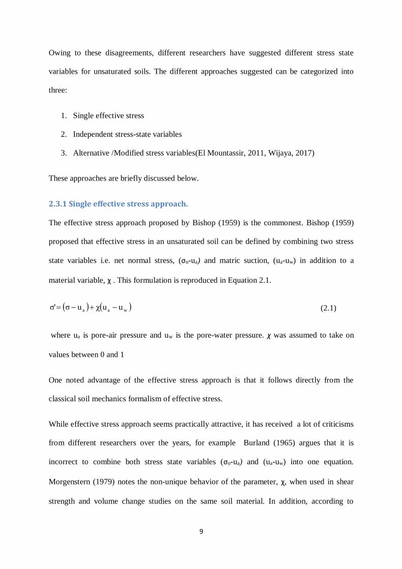
The effective stress approach proposed by Bishop (1959) is the commonest. Bishop (1959)

proposed that effective stress in an unsaturated soil can be defined by combining two stress

state variables i.e. net normal stress, (σn-ua) and matric suction, (ua-uw) in addition to a

material variable, χ . This formulation is reproduced in Equation 2.1.

waa uuχuσσ' (2.1)

where ua is pore-air pressure and uw is the pore-water pressure. χ was assumed to take on

values between 0 and 1

One noted advantage of the effective stress approach is that it follows directly from the

classical soil mechanics formalism of effective stress.

While effective stress approach seems practically attractive, it has received a lot of criticisms

from different researchers over the years, for example Burland (1965) argues that it is

incorrect to combine both stress state variables (σn-ua) and (ua-uw) into one equation.

Morgenstern (1979) notes the non-unique behavior of the parameter, χ, when used in shear

strength and volume change studies on the same soil material. In addition, according to

10

Morgenstern (1979), χ, being a material variable cannot be part of a stress state variable.

Further, Morgenstern (1979) notes that the χ parameter can exceed one especially in the low

suction which is incompatible with theoretical expectations. Bishop et al. (1960) and Jennings

and Burland (1962) have further noted the difficulty in determining χ experimentally.

Despite these challenges, some proponents for the effective stress approach exist, for example

Khalili and Khabbaz (1998) established an empirical relationship for χ with suction ratio

a w

a w b

u u

u u

given in Equation 2.2 for 14 soils at a coefficient of correlation of 0.94.

bwawa

bwawa

55.0

bwa

wa

uuuufor 1

uuuufor uu

uu

χ (2.2)

where bwa uu = air entry value of the soil.

According to Khalili and Khabbaz (1998), Equation 2.2 is sufficient for practical purposes.

2.3.2 Independent stress state variable approach

The proponents of this approach arise owing to the difficulties of using the effective stress

approach. In this approach, different combinations of stress state variables are used to

describe the behavior of unsaturated soils. According to Fredlund and Morgenstern (1977),

any two of three possible state variables: σ, uw, ua are sufficient in defining the stress state of

unsaturated soils. This therefore leads to the following possible combinations of stress state

variables:

1. (σ-ua) and (ua-uw)

2. (σ-uw) and (ua-uw)

11

3. (σ-ua) and (σ-uw)

According to Fredlund et al. (2012), of the three combinations, the combination of net normal

stress, (σ-ua) and matric suction, (ua-uw) has received the widest acceptance in describing

behavior of unsaturated soils. This is because the pair allows for separation of the influences

of total stress and pore-water pressure. In addition, since pore-air pressure is usually

atmospheric, it makes practical advantage to have stress variables that are referenced to pore-

air pressure (El Mountassir, 2011).

Some of the critics of this approach like Khalili and Khabbaz (1998) note that this approach

requires extensive testing which is very time consuming. In addition the test equipment used

to obtain the unsaturated soil properties is often very expensive and highly sophisticated.

Khalili and Khabbaz (1998) further note that the highly non-linear relationship between

band soil suction limits the field application of the approach to only a small suction range

often tested in the laboratory. Because of these limitations, Khalili and Khabbaz (1998) note

that the method is not widely applied in practice.

2.3.3 Alternative /Modified stress variables approach

This approach combines both the effective stress approach and the independent stress

approach. According to Wijaya (2017), this approach modifies the independent stress state

variables with material properties hence generating modified stress state variables to describe

the behavior of unsaturated soils

The proponents of this approach seek to investigate the independent contribution of degree of

saturation and suction to the behavior of unsaturated soils. According to Wheeler et al.

(2003), ignoring the independent influence of degree of saturation is not correct especially

considering the hydraulic hysteresis of SWCC.

12

Wheeler et al. (2003) modified the work- conjugate stress variables of net stress, σv and

suction, s suggested by Houlsby (1997) into two variables shown in Equation 2.3

rv

''

v sSσσ (2.3a)

nss* (2.3b)

where: ''

vσ = average skeleton stress, *s = modified suction, n = instantaneous porosity and Sr=

degree of saturation.

Similarly, Alonso et al. (2013) suggested a constitutive stress, , and effective suction, s , to

model the behavior of unsaturated soils. These stress variables are defined in Equation 2.4

su-σ a (2.4a)

*

rsS s (2.4b)

where σ = total stress, ua = pore-air pressure, s = matric suction, Sr*= effective degree of

saturation.

The effective degree of saturation has been defined by Romero and Vaunat (2000) and

Tarantino and Tombolato (2005) in terms of a material variable, mξ as shown in Equation 2.5

mr

*

r

mr

m

mr*

r

ξSfor 0S

ξSfor ξ1

ξSS

(2.5)

where; Sr = degree of saturation

The material variable, mξ is defined as a ratio of microstructural void ratio, em to the total

void ratio, e i.e. em/e

13

Gens et al. (2006) generalized the constitutive stress and modified suction as shown in

Equation 2.6

s,.....μ )u-(σ 1a (2.6a)

s,.....μ 2 (2.6b)

From Equation 2.6a, Gens et al. (2006) suggests three possible cases depending on the

expression of 1μ i.e

1. 0μ1 ; Equation 2.6a becomes the net normal stress

2. )(sμ1 ; Equation 2.6a is a function of suction and not degree of saturation

3. )S(s,μ r1 ; Equation 2.6a is a function of both suction and degree of saturation which

in turn is equivalent to the average skeleton stress given in Equation 2.3a

Similarly, different cases can be constructed out of Equation 2.6b

1. (s) μ 2 ; if Equation 2.6b is a function of suction only, then it becomes matric suction

only.

2. s)(n,μ2 ; if Equation 2.6b is a function of n and s, then it becomes modified suction as

shown in Equation 2.3b

3. )S(s,μ r2 ; if Equation 2.6b is a function of both suction and degree of saturation, it

becomes effective suction as shown in Equation 2.4b

Usage of alternative stress state variables is receiving a lot of attention in the research

community. One of its advantages is the ability to use conventional equipment in testing and

also the fact that the testing is much less intensive compared to the independent stress state

variable approach (Tarantino and El Mountassir, 2013).

14

2.4 Soil Suction

Soil suction is an important stress variable for unsaturated soils. There are two major

components of soil suction (total suction) i.e., matric and osmotic suctions.

2.4.1 Definitions of suction

Aitchison (1964) defines the different components of soil suction as:

Matric suction or capillary component of free energy:

“In suction terms, it is the equivalent suction derived from the measurement of the partial

pressure of the water vapour in equilibrium with the soil water, relative to the partial pressure

of the water vapour in equilibrium with a solution identical in composition with the soil

water.”

Osmotic (or solute ) component of free energy:


pressure of the water vapour in equilibrium with a solution identical in composition with the

soil-water, relative to the partial pressure of the water vapour in equilibrium with free pure

water.”

Total suction or free energy of soil-water


pressure of the water vapour in equilibrium with the soil-water, relative to the partial pressure

of water vapour in equilibrium with free pure water.”

2.4.2 Matric suction

Matric suction is commonly expressed as the difference between pore-air and pore-water

pressures (Fredlund and Rahardjo, 1993) as shown in Equation 2.7

15

wa uu (2.7)

According to El Mountassir (2011), matric suction is the affinity of the solid phase of soil for

water which arises from the water retention mechanisms.

In granular materials where chemical interactions between solids and soil water hardly exist,

capillary effects are the dominant contribution of matric suction. In clayey soils, capillary

forces play a significant role in the low suction range (Tuller et al., 1999; Tuller and Or,

2005). In the higher suction range (low degrees of saturation), surface adsorptive forces

dominate (Tuller et al., 1999; Tuller and Or, 2005).With surface adsorption, the water is held

as films covering the solid particles. The thickness of the films depends on the surface

adsorptive forces. Figure 2.3 presents a simplified schematic showing water films covering

soil particles in a surface adsorption process.

Surface adsorption of the pore water is controlled by physico-chemical aspects which

include; i) van der Waal’s forces, ii) electrostatic forces and iii) hydration forces (Tuller et al.,

1999; Tuller and Or, 2005; Tarantino, 2010)

The physico-chemical aspects responsible for the surface adsorptive forces are controlled by

the mineralogy of the clay as well as the surface properties of the clay particles (Tuller et al.,

1999; Tuller and Or, 2005)

Baker and Frydman (2009) note that in order to improve the constitutive models used for

unsaturated soils, it is important to consider the contributions of both capillarity and surface

adsorption to matric suction.

16

Figure 2.3: Schematic illustration of water adsorption on clay particle surafces (from Baker and

Frydman, 2009)

2.4.3 Total suction

According to Tarantino (2010), water can be transferred from the soil via vapour when the

partial water vapour pressure in equilibrium with soil pore water pressure gets lower than the

water vapour pressure in equilibrium with pure free water. The depression of the soil water

vapour pressure is due to two mechanisms: i) negative pressure of soil water and ii) solute

concentration of soil water (Tarantino, 2010).

The Poynting effect explains that the pressure of the vapour in equilibrium with its own

liquid reduces as the liquid pressure decreases where the decrease in the liquid pressure is

generated by the solid phase (Tarantino, 2010). On the other hand, Raoult’s law shows that

the pressure of vapour in equilibrium with an aqueous solution decreases as the solute

concentration increases. Therefore, total suction is generated by both the solid phase (matric

17

suction) and the solute concentration (osmotic or solute suction). Equation 2.8 shows the

mathematical relationship between the three forms of suction

πuuψ wa (2.8)

where: ψ= total suction, (ua-uw) = matric suction and π = osmotic suction

The thermodynamic relationship of the free energy of the soil water (total suction) and the

relative humidity is expressed in Kelvin’s law given in Equation 2.9.

0w P

Pln

M

RTψ (2.9)

where: R = universal molar gas constant i.e., 8.31432J/(mol K), T = absolute temperature,

Mw= molecular mass of water (kg/mol), 0P

P= relative humidity of air in equilibrium with

soil water.

For many applications in unsaturated soil mechanics, much focus is given to matric suction

while ignoring osmotic suction partly because osmotic suction is a much smaller value

compared to matric suction. In addition, for non-active soils, osmotic effects are likely to be

negligible (Gens, 2010)

2.4.4 Suction control and measurements

In the practice of unsaturated soil mechanics, very often, there is need to either control or

measure suction depending on the application. The different techniques used in the control

and measurement of suction are briefly presented below.

18

2.4.4.1Techniques for controlling suction

a) Axis-translation technique

For unsaturated soils, it is typical that pore-air pressure is atmospheric i.e., ua = 0 while the

pore- water pressures are negative with respect to atmospheric pressure. Hilf (1956) proposed

the axis- translation technique which translates the origin of reference for the pore-water

pressure from standard atmospheric condition to the air pressure applied (Fredlund et al.,

2012). Because of this translation, the problem of cavitation in laboratory test is avoided.

Cavitation occurs when water is brought to a suction of -100kPa relative to the atmospheric

pressure.

In a laboratory test employing this technique, the air pressure is applied inside an air-tight

chamber and separation of the air phase from the water base is achieved using a water

saturated disk of low porosity. This disk which is made of ceramic is often referred to as high

air-entry value (HAEV) porous disk. The HAEV disks are often defined by their air-entry

values (AEVs) or the air pressures that they are able to withstand before they start to

desaturate. In the laboratory, typical HAEV disks have AEVs of 100, 500, and 1500kPa.

The reference pore-air pressure is elevated through an artificial increase while maintaining

the pore-water pressure at some measurable reference value typically atmospheric (Delage et

al., 2008; Lu and Likos, 2004).The matric suction wa uu can then be controlled over a

wide range.

19

a) Principle of axis translation (after El

Mountassir, 2011)

b) A typical pressure plate

extractor applying axis-

translation technique (after

Samingan 2005)

Figure 2.4: Illustration of the axis-translation technique

The axis-translation technique has been criticized concerning the following aspects: i) it is

not representative of field conditions where air pressure is under atmospheric condition; ii)

there are some doubts in how the air pressurization process affects the water pressure when

water is held by adsorption mechanisms; and finally iii) its application at nearly saturated

states in the absence of a continuous gaseous phase is not straightforward (Delage et al.,

2008); Baker and Frydman (2009).

The major experimental difficulties concerning the application of the axis-translation

technique are associated with: i) the accumulation of diffused air beneath the HAEV disk, ii)

the control of the relative humidity of the air chamber to minimize evaporation or

condensation effects on the sample, iii) the application of the air pressurization process at

elevated degrees of saturation, and iv) the estimation of the equalization time (Delage et al.,

2008).

Despite these challenges, the axis-translation technique is the most commonly used technique

of controlling suction. The technique is frequently used in determining the lower suction

20

range of the soil-water characteristic curve (usually less than 1500kPa). It has also been

applied to several test apparatuses, for example Bishop and Donald (1961) designed the first

suction-controlled triaxial apparatus using the axis-translation technique, Escario (1969) and

Hoffmann et al. (2005) designed suction-controlled oedometers based on axis-translation

technique to study swelling and expansive soils, respectively. Direct shear boxes with suction

control using axis-translation technique have been developed by researchers such as Escario

(1986) and Gan et al. (1988).In this thesis, the axis-translation technique has been applied to

measure the SWCCs of the compacted soils.

b) Vapour equilibrium technique

In this technique, the relative humidity of a closed system (usually desiccators) is controlled

using a chemical solution for example, a saline solution or an acid. When a soil specimen is

placed in the desiccators as illustrated In Figure 2.5, water exchanges occur by vapour

transfer between the pore water in the soil specimen and the aqueous solution until

equilibrium is reached.

Figure 2.5: Vapor equilibrium technique (from Leong and Rahardjo, 2002)

According to Leong et al. (2002b) equilibration is in two stages; initially equilibrium has to

be achieved between the suction source (chemical solution) and the environment (vapour

space). This occurs through net water exchange between the liquid and vapour phases until

Desiccator

Porcelain

crucibles

Soil

specimens

Salt solution

21

equilibrium is achieved (Blatz et al., 2008).The second stage involves equilibration between

the soil specimen and the vapour space through an exchange of water.

The partial vapour pressure in the closed environment is directly related to the concentration

of the aqueous solution. Both unsaturated and saturated salt solutions have been used by

various researchers. However saturated solutions are usually preferred because the

concentration of the solution remains almost constant despite the exchange of water between

the soil specimens and the environment (Blatz et al., 2008; Young, 1967). Several works have

published relative humidity levels generated by various salt solutions (Tang and Cui, 2005;

Young, 1967). This technique is very easy to use and very high suctions in the range of 3-

1000MPa can be reached (Pintado et al., 2009).

The vapour equilibrium technique has some setbacks which include:

Long time for equilibrium as the equilibrium is a two-stage diffusion process.

Strict control on temperature. Slight variations in temperature can cause dramatic

changes in suction (Blatz et al., 2008). Blatz et al. (2008) suggests using water baths

to minimize temperature variations.

Not accurate at low suction levels (Agus and Schanz, 2005)

Errors can be introduced during mixing of solution due to incomplete dissolution of

solute, spillage of water, loss of water through evaporation and possible scale

calibration errors (Blatz et al., 2008)

In this thesis, this technique has been used to attain high suctions in the test samples which

will be discussed subsequently.

22

c) Osmotic technique

The osmotic technique was developed by biologists and was later adopted by soil scientists

and then introduced to geotechnical engineering by Kassiff and Shalom (1971). In this

technique the soil specimen is separated from an aqueous solution of large sized

polyethyleneglycol (PEG) molecules by a semi-permeable membrane. Water transfer or

exchange takes place across the semi-permeable membrane by the process of osmosis. The

most commonly used semi-permeable membranes are cellulose membranes (Delage and Cui,

2008).Semi-permeable membranes are characterised by their molecular weight cut-off which

is linked to the PEG molecules sizes (Delage et al., 2008). It is therefore important that the

correct membrane is used for the PEG molecule size used in the experiments so that no

exchange of PEG molecules takes place between the soil specimen and the aqueous solution.

The water transfer takes place in liquid phase and ions can freely cross the semi-permeable

membrane hence the osmotic technique controls matric suction of the soil and not osmotic

suction (Blatz et al., 2008; Delage et al., 2008; Delage and Cui, 2008).Figure 2.6 illustrates

how suction is imposed on a soil specimen using the osmotic technique.

Figure 2.6: Application of the osmotic technique to impose suction on a soil sample (from Cui

and Delage, 1996)

23

One advantage of the osmotic technique is that matric suction can be imposed on a soil

sample without the need for applying an air pressure as in the case with the axis-translation

technique (Delage and Cui, 2008; Delage et al., 2008). Avoidance of the air pressure has

safety advantages but most importantly ensures that the samples are tested in conditions close

to their natural conditions. Secondly, relatively high matric suctions (as high as 10MPa)

(Delage et al., 2008) can be attained by the osmotic technique, which are not easily attained

by the axis-translation technique. Matric suctions are adjusted by adjusting concentration of

the PEG solution. The higher the concentration of the PEG solution, the higher will be the

imposed matric suction. Because high suctions can be achieved in addition to the ability to

apply a direct water potential to liquid water which is not the case in axis translation (Blatz et

al., 2008), osmotic technique is suitable for high water content samples (Blatz et al., 2008).

The major setback of the osmotic technique is the durability of the membrane. The membrane

is usually weak and very susceptible to microbial attack. In order to overcome the problem of

microbial attack, a few drops of an antibiotic like penicillin into the aqueous solution are

recommended (Delage et al., 2008). Some testing devices have been designed based on this

technique, for example, Dineen and Burland (1995) designed an oedometer that is

osmotically controlled and an osmotic direct shear box has been designed by Boso et al.

(2005).

2.4.4.2 Suction measurement techniques

Several methods for suction measurement exist in the literature. Three common methods i.e.,

high capacity tensiometer, chilled mirror dewpoint technique and filter paper technique are

presented below. Other methods are summarised in Table 2.1.

24

a) High capacity tensiometer

The high capacity tensiometer (HCT) is a direct method of measuring matric suction.

Tensiometers measure matric suction by directly measuring negative pore-water pressure

while pore air pressure is atmospheric. Tensiometers were for a long time limited to

measure maximum suctions in the range 70-80kPa due to the limitation of cavitation.

However following Ridley and Burland (1993)’s work, a tensiometer with capacity to

measure suctions as high as 1500 kPa was invented hence the description high capacity

tensiometer. Figure 2.7 shows a high capacity tensiometer.

Figure 2.7: High Capacity tensiometer (after Ridley et.al, 2003)

A HCT typically consists of three components: i) high air entry value (HAEV) ceramic

porous disk, ii) water reservoir/chamber, iii) strain/pressure gauge.

The HAEV ceramic disk acts as an interface between the negative water pressure in the soil

and the measuring system (Fredlund et al., 2012). When the HAEV ceramic porous disk is in

intimate contact with the pore water, exchange of water between the water reservoir and the

soil occurs until equilibrium is reached. The strain gauge which is attached to the reservoir is

designed to detect these movements (due to water exchange) hence determining the soil

suction directly.

25

The main drawback of a HCT is cavitation. If cavitation occurs during the process of suction

measurement, the measurement is disrupted and the system will need re-saturation. Therefore

cavitation plays an important role in the design and operation of the HCT (Tarantino and

Mongiovì, 2001). Some of the design considerations to limit cavitation include having a

small water reservoir which reduces the chances of bubble formation in the reservoir,

minimizing surface roughness/ imperfections on the ceramic disk in order to ensure good

contact with the soil sample under test (Ridley et al., 2003).

Some of the precautions necessary when conducting suction measurements with a HCT

include saturation of the ceramic porous disk and water reservoir prior to each testing,

removal of air using a vacuum, ensuring good contact between the soil sample and the

ceramic porous disk. Detailed procedures regarding operation of the HCT are presented in

Tarantino and Mongiovì (2001), Tarantino and Mongiovi (2003), and Ridley et al. (2003).

Successes of the application of HCT in geotechnical testing have been variably reported,

although majority are among the research community. Laboratory equipment have been

designed to incorporate tensiometers for example: in oedometers (Wijaya, 2017), in direct

shear testing (Caruso and Tarantino, 2004), triaxial testing (Marinho et al., 2016). Meilani et

al. (2002) used mini-suction probes to successfully measure suctions up to 400kPa along the

height of a test specimen during a triaxial test.

The main advantage of the tensiometer is the ability to measure suction directly in a short

time. Being a direct method of suction measurement, it is suitable in validating indirect

methods of suction measurement (Tarantino and Mongiovì, 2001).

26

b) Chilled mirror dew-point technique

This is an indirect suction measurement method that makes use of vapour pressure to

determine total suction. The technique is useful for samples drier than the axis translation or

ordinary tensiometric suction range (Campbell et al., 2007). ASTM D6836-16 recommends

the technique for suctions higher than 1000kPa. In addition to capacity to measure high

suctions, the technique takes a short time to attain equilibrium and hence total suction

measurement (Gee et al., 1992; Leong et al., 2003).While measuring the total suction of

compacted soils, Leong et al. (2003) noted that equilibrium was attained between a couple of

minutes and 18 minutes. Agus and Schanz (2005) compared four methods for total suction

measurement and noted that the chilled mirror hydrometer technique was the most accurate

of them and recommended it as a bench mark against which other sensors can be assessed.

The chilled-mirror dewpoint hygrometer is shown schematically in Figure 2.8.

Figure 2.8: A schematic of the chilled-mirror dewpoint hygrometer (after Leong et al., 2003).

The chilled-mirror dewpoint hygrometer measures dew point and temperature of the

headspace above the specimen. The specimen in a small plastic container (occupying half the

container) is placed in a special closed chamber. The dew point is measured using a mirror

which can detect the first appearance of condensation of water vapor. In order to maintain a

constant thickness of the dew, the temperature of the mirror is precisely controlled by a

thermoelectric cooler. A light beam directed onto the mirror is used to detect the first

27

appearance of water vapor condensation. A photo-detector cell is employed to measure the

change in reflectance of the mirror caused by the condensed water vapor. The temperature of

the specimen which is considered to be equal to the temperature of the vapor space is

measured via an infrared thermocouple. The relative humidity or the water activity of the

specimen is computed from the measured dew point and temperature. An internal fan is used

to speed up equilibration time. The internal fan circulates the water vapor in the vapor space

above the specimen. With the water activity or relative humidity and temperature of the vapor

space above the soil specimen known, the total suction of the soil specimen is computed

using Kelvin’s Law given in Equation 2.9. Prior to usage, the chilled-mirror dewpoint

hygrometer is calibrated using standard aqueous salt solutions whose relative humidity and

hence total suctions are known.

In this thesis, the chilled-mirror dewpoint hygrometer was used to measure suctions both in

the low and high ranges.

c) Filter paper technique

Usage of the filter paper technique as a soil suction measurement tool was first reported by

Gardner (1937). Substantial studies have been made to improve understanding of this

technique (Bulut et al., 2001; Bulut and Leong, 2008; Al-Khafaf and Hanks, 1974; Marinho

and Oliveira, 2006; Marinho and da Silva Gomes, 2012; Haghighi et al., 2012; Bicalho et al.,

2007; Bicalho et al., 2008; Likos and Lu, 2002). In addition, the technique has been

standardized in ASTM D5298-16. Only ash-less filter papers are used for this technique

(Bicalho et al., 2007). Despite the fact that several ash-less filter papers exist, the two

commonly used filter papers for soil suction measurements are the Whatman No. 42 and the

Schleicher and Schuell No. 589.

28

In all the studies, it was generally agreed that this technique is economical, relatively simple

to use, gives fairly reliable measurements, measures suctions over a wide range, and

measures both matric and total suctions.

The different aspects of the technique are briefly presented below.

Contact and Non-contact filter paper

Several researchers (e.g., Swarbrick 1995; Leong et al. 2002b; Marinho and Oliveira 2006)

have detailed the working principles of the filter paper technique. The filter paper method has

also been standardized in ASTM D-5298-16.

The filter paper can be used in the contact or non-contact mode. If placed in direct contact

with soil, moisture exchange between the filter paper and soil takes place through capillary

flow and hence the contact filter paper measures matric suction. If the filter paper is not in

contact with the soil but placed together in a sealed environment, moisture exchange between

the filter paper and soil takes place through vapor flow and hence the non-contact filter paper

measures total suction.

Once the filter paper is in equilibrium with the soil’s suction, its weight is expected to remain

constant. Suction can then be inferred from the water content of the filter paper using a

calibration equation. Calibration involves establishing the moisture-suction relationship of the

filter paper.

Several calibration curves for filter papers exist in the literature for example: Fawcett and

Collis-George (1967), Hamblin (1981), Chandler and Gutierrez (1986), and Leong et al.

(2002b).A detailed discussion of filter paper calibration procedures is presented by Leong et

al. (2002b). The contact and non-contact filter paper are calibrated by allowing moisture

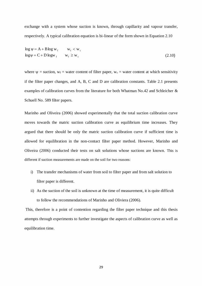
29

exchange with a system whose suction is known, through capillarity and vapour transfer,

respectively. A typical calibration equation is bi-linear of the form shown in Equation 2.10

cff

cff

w wlogw DClogψ

w wwlogBAψlog

(2.10)

where = suction, wf = water content of filter paper, wc = water content at which sensitivity

if the filter paper changes, and A, B, C and D are calibration constants. Table 2.1 presents

examples of calibration curves from the literature for both Whatman No.42 and Schleicher &

Schuell No. 589 filter papers.

Marinho and Oliveira (2006) showed experimentally that the total suction calibration curve

moves towards the matric suction calibration curve as equilibrium time increases. They

argued that there should be only the matric suction calibration curve if sufficient time is

allowed for equilibration in the non-contact filter paper method. However, Marinho and

Oliveira (2006) conducted their tests on salt solutions whose suctions are known. This is

different if suction measurements are made on the soil for two reasons:

i) The transfer mechanisms of water from soil to filter paper and from salt solution to

filter paper is different.

ii) As the suction of the soil is unknown at the time of measurement, it is quite difficult

to follow the recommendations of Marinho and Oliviera (2006).

This, therefore is a point of contention regarding the filter paper technique and this thesis

attempts through experiments to further investigate the aspects of calibration curve as well as

equilibration time.

30

Hysteresis

The moisture retention characteristics of a porous material have been observed to differ

depending on whether the material is wetting or drying. This phenomenon is called hysteresis

and applies to the filter paper as well. Previous studies (Fawcett and Collis-George 1967;

Leong et al. 2002b; 2016) have demonstrated presence of the hysteretic behavior of filter

paper. Al-Khafaf and Hanks (1974), Ridley (1995) and Swarbrick (1995) therefore

recommend that the calibration process of filter papers should always take into account the

hysteresis effect. Consequently, in the usage of the filter paper to evaluate suction, the

appropriate calibration curve should be used to infer suction from the filter paper. Not much

experimental data exists on the hysteretic behavior of the filter paper. This is partly because

most experimenters use an initially dry filter paper and so the filter paper moves along the

wetting path as it measures the soil suction. As part of this study, the hysteretic behavior of

filter papers using both initially dry and initially wet filter papers was investigated.

Inherent variability of the filter papers

Filter papers are produced in batches. Some researchers e.g. Deka et al. (1995) recommend

that each batch of filter papers should be calibrated for the entire range of suction they are to

be used. This suggestion is not practical and hence Marinho and Oliveira (2006) have

suggested a quick single point check for verification of the calibration curve to apply.

Hamblin (1981) compared calibration data of Whatman No.42 papers calibrated two years

apart in addition to data from Fawcett and Collis-George (1967), 14 years apart and found the

data closely agreed. Leong et al. (2002b) have investigated quality of both the Whatman

No.42 and the S &S 589 filter papers for the probable influence on the calibration of filter

papers. Using their own data, in addition to published data, Leong et al. (2002b) concluded

that the variation was minimal, and does not practically affect the calibration data. The

31

calibration data combined all lay in reasonably narrow band with more uniformity in the case

of Whatman No.42 filter papers as shown in Figure 2.9 after Rahardjo and Leong (2006).

Therefore unless extremely special situations arise, entire re-calibration of the filter papers

may be practically unnecessary but rather may increase the time duration for the tests. It is

important to ensure proper handling of the filter papers and provide sufficient equilibration

time as suggested by Leong et al (2002b).

Equilibration time

Equilibration time is an important aspect for any suction measurement technique. Different

studies have suggested that the equilibration time for filter papers is dependent on the mode

of contact (contact or non-contact), the magnitude of suction being measured and the soil

characteristics (Swarbrick, 1995; Marinho and Oliveira, 2006; Marinho and da Silva Gomes,

2011). ASTM D5298-16 recommends a minimum of seven days. As part of this study, the

equilibration time was investigated and suggestions were made.

Pre-treatment of the filter papers

Different researchers (Gardner, 1937; McQueen and Miller, 1968; Al-Khafaf and Hanks,

1974) have suggested chemical pre-treatment of filter papers prior to usage. The main reason

for pre-treating the filter papers is to avoid microbial attack of the filter papers during testing.

In some cases for example Fawcett and Collis-George (1967), both chemical pre-treatment

and oven-drying of the filter papers were done prior to the usage. ASTM D5298-16 suggests

oven drying of filter papers prior to use. In addition, ASTM D5298-16 suggests usage of

sacrificial filter papers in order to avoid microbial attack. Usage of sacrificial filter papers

extends the equilibration time and needs to be studied. Hamblin (1981) and Chandler and

Gutierrez (1986) reported that pre-treatment of filter papers is not necessary. Marinho and

Oliveira (2006) note that pretreatment of the filter papers alters their absorption

32

characteristics and hence requires different calibration curves. In this study, the filter papers

were not pre-treated and no sacrificial filter paper was used.

33

Table 2.1: Suction control and Suction measurement techniques (Ridley and Wray, 1996; Blatz et al, 2008; Bulut and Leong, 2008; Masrouri et al,

2008; Vanapalli et.al, 2008)

SC/SM* Technique Suction

component

Suction

range

MPa

Approx.

Equilibration time

Concerns

SC Axis translation Matric 0-1.5 days-weeks Requires elevated air pressures, air diffusion through

ceramic, saturation of ceramic is crucial, evaporation

of soil sample.

SC Vapour equilibrium Total 3-1000 weeks –months Long test durations, sensitive to temperature

fluctuations, safety if acids are used

SC Osmotic Matric 0-10 days-weeks Deterioration of membranes

SC Centrifuge Matric 0-0.08 days Narrow suction range

SC Hanging water

column

Matric 0-0.12 hours Narrow suction range

SM Tensiometer Matric 0-1.5 minutes-hours Rigorous saturation required

SM Chilled-mirror

dewpoint

Total 1-60 10 minutes Regular calibration, only a small amount of soil is

tested

SM Filter paper Matric/Tota

l

0.05-30 7 days- A strict protocol, very dependent on workmanship

skills

SM Thermocouple

psychrometer

Total 0.3-7 ~1hr Sensitive to ambient temperature changes

SM Transistor

psychrometer

Total 1-70 ~1hr Sensitive to ambient temperature, only a small soil

specimen is tested

SM Thermal conductivity

sensor

Matric 0.001-1.5 hours-days Different calibration for each sensor, Shows hysteresis

on drying and wetting, contact between soil and sensor

affects response

SM Electrical conductivity

sensor

Matric 0.05-1.5 6-50 hours Not suitable in saline soils since gypsum block may

get corroded, suffers from hysteresis

*SC = Suction control, SM = Suction measurement

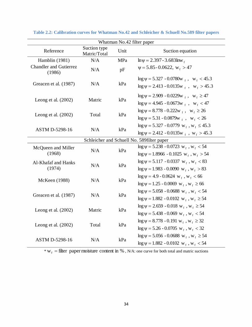
34

Table 2.2: Calibration curves for Whatman No.42 and Schleicher & Schuell No.589 filter papers

Whatman No.42 filter paper

Reference Suction type

Matric/Total Unit Suction equation

Hamblin (1981) N/A MPa f3.683lnw-2.397lnψ

Chandler and Gutierrez

(1986) N/A pF 47 w0.0622,-5.85ψ f

Greacen et al. (1987)

N/A

kPa 3.45 w, 0.0135w-2.413logψ

45.3 w, 0.0780w-5.327logψ

f f

ff

Leong et al. (2002) Matric kPa 47 w, 0.0673w-4.945logψ

47 w, 0.0229w-2.909logψ

f f

ff

Leong et al. (2002) Total kPa 26 w, 0.0879w-5.31logψ

26 w, 0.222w-8.778logψ

f f

ff

ASTM D-5298-16 N/A kPa 3.45 w, 0.0135w-2.412logψ

45.3 w, w0.0779-327.5logψ

f f

ff

Schleicher and Schuell No. 589filter paper

McQueen and Miller

(1968) N/A kPa

54 w, w0.1025-1.8966logψ

54 w, w0.0723-5.238logψ

f f

ff

Al-Khafaf and Hanks

(1974) N/A kPa

83 w, w0.0090-1.983logψ

83 w, w0.0337-5.117logψ

f f

ff

McKeen (1988) N/A kPa 66 w, w0.0069-1.25logψ

66 w, w0.0624-4.9logψ

f f

ff

Greacen et al. (1987) N/A kPa 54 w, w0.0102-1.882logψ

54 w, w0.0688-5.058logψ

f f

ff

Leong et al. (2002) Matric kPa 54 w, w0.069-5.438logψ

54 w, w0.018-2.659logψ

f f

ff

Leong et al. (2002) Total kPa 32 w, w0.0705-5.26logψ

32 w, w0.191-8.778logψ

f f

ff

ASTM D-5298-16 N/A kPa 54 w, w0.0102-1.882logψ

54 w, w0.0688-5.056logψ

f f

ff

* %in content moisturepaper filter w f , N/A: one curve for both total and matric suctions

35

(a) Whatman No.42 filter papers

(b) Schleicher and Schuell No.589 filter papers

Figure 2.9: Calibration data for the filter papers from different researchers (from Rahardjo and

Leong, 2006)

36

2.5 Soil-water characteristic curves

The soil-water characteristic curve (SWCC) is a graphical relationship between the amount of

water in the soil and the soil suction (Fredlund and Rahardjo, 1993).The amount of water in the

soil can quantified as either gravimetric water content (w), volumetric water content (θw) or

degree of saturation (S). Hence, the SWCCs may be designated according to the form of water

content used to describe it i.e. SWCC-w, SWCC-θw or SWCC-S.

Depending on the discipline, the soil-water characteristic curve takes on different names for

example water retention curve, soil-moisture retention curve, soil-water release curve and soil-

moisture characteristic curve. For civil engineering purposes, the term soil-water characteristic

curve (SWCC) is recommended (Fredlund et al., 2002). Figure 2.10 shows a typical drying

SWCC showing the different variables and zones.

Figure 2.10: Drying SWCC showing the variables and the different zones(Fredlund, 2006)

37

Air entry value (AEV) is the matric suction at which air starts to enter the largest pores of the

soil (Fredlund and Xing (1994). At this suction, the meniscus formed by the water surface

tension in the largest pores is broken (Zhai and Rahardjo, 2012). Residual water content is the

water content that requires a large suction to remove any additional water from the soil (Fredlund

et al., 2012). The AEV and the residual water content are usually determined empirically by

constructing a tangent through the point of inflection as shown in Figure 2.10 for a non-

deforming soil; the point of intersection of this tangent and the horizontal tangent through the

initial point is the AEV. In order to obtain the residual water content, a line extending from zero

water content and 1GPa suction is drawn to intersect the tangent line through the point of

inflection; the residual water content is the ordinate at the point of intersection of these two

tangents as illustrated in Figure 2.10 (Vanapalli et al., 1998). Because the empirical approaches

can be subjective when determining the SWCC variables, mathematical formulations have been

suggested by Zhai and Rahardjo (2012).

The SWCC is very important in the implementation of unsaturated soil mechanics (Fredlund et

al., 2002). The SWCC provides primary information for derivation of many unsaturated soil

properties such as shear strength, permeability, pore size distribution either directly or indirectly.

In the laboratory, SWCC is measured by different methods for example hanging column,

pressure extractor, chilled mirror hygrometer and centrifuge which have been standardized in

ASTM D6836-16. Other techniques used are vapour equilibrium technique and filter paper

technique which have been previously described. For most applications, only the drying SWCC

is sufficient, however it is important to note that the SWCC is hysteretic i.e., the SWCC follows

a different path during drying and during wetting processes of the soil. Figure 2.11 shows both

the drying (desorption) curve and the wetting (absorption) curve of a silt soil.

38

Along the drying path, the suction is increasing hence leading to desorption, while wetting

occurs under suction reduction hence leading to water absorption by the soil. The measurement

of the wetting curve is quite cumbersome and more time consuming hence much less data exists

for wetting SWCC compared to the drying SWCC, moreover drying SWCC seems sufficient in

explaining or modeling majority of the phenomena in unsaturated soil.

Figure 2.11: Typical SWCC for a silt soil (from Fredlund et al, 2012)

White et al. (1970) idealized the desorption curve of a porous material into four regions i.e.,

boundary effect zone, primary transition zone, secondary transition zone and residual

desaturation zone. Vanapalli et al. (1996a) modified these regions into three as shown in Figure

2.10: boundary effect zone, transition zone (originally primary and secondary transition zones)

and the residual zone. In the boundary effect zone, the pores are filled with water i.e., the water

phase is continuous making the soil saturated. Therefore in the boundary effect zone, the

effective stress, (σ-uw) is applicable as stress state variable. At the AEV, the soil starts to

desaturate, making AEV the first most significant point on the SWCC (Vanapalli et al., 1996a).

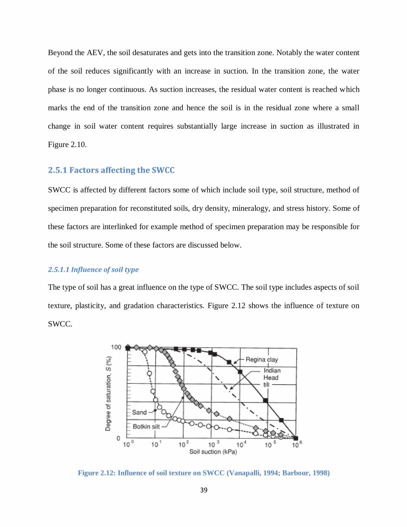
39

Beyond the AEV, the soil desaturates and gets into the transition zone. Notably the water content

of the soil reduces significantly with an increase in suction. In the transition zone, the water

phase is no longer continuous. As suction increases, the residual water content is reached which

marks the end of the transition zone and hence the soil is in the residual zone where a small

change in soil water content requires substantially large increase in suction as illustrated in

Figure 2.10.

2.5.1 Factors affecting the SWCC

SWCC is affected by different factors some of which include soil type, soil structure, method of

specimen preparation for reconstituted soils, dry density, mineralogy, and stress history. Some of

these factors are interlinked for example method of specimen preparation may be responsible for

the soil structure. Some of these factors are discussed below.

2.5.1.1 Influence of soil type

The type of soil has a great influence on the type of SWCC. The soil type includes aspects of soil

texture, plasticity, and gradation characteristics. Figure 2.12 shows the influence of texture on

SWCC.

Figure 2.12: Influence of soil texture on SWCC (Vanapalli, 1994; Barbour, 1998)

40

Figure 2.12 shows variations in the SWCC slopes and AEV with fines content. The AEV

generally reduces from Regina clay to sand. The slope of the SWCC in the transition zone is

steepest in sand reducing toward Regina clay. These observations are largely due to the

differences in pore sizes across the different soil textures. The shape of the SWCC for sand

reveals a uniform pore size distribution which becomes gentler as clay content increases.

As discussed earlier, the water retention mechanisms in cohesive and cohesionless soils are

different. In cohesive soils, both capillary and surface adhesion forces are present while in

cohesionless soils, capillary forces are the most significant. This may explain why the sands and

silts desaturate much faster than clays.

Marinho (2005) notes that the slope of the SWCC transition zone changes with liquid limit; for

soils with liquid limits above 25%, the SWCC is a straight line between suctions of 100 and

10000kPa. Lu et al. (2007) studied the relationship between plasticity and water retention

behavior and concluded that the higher the plasticity index, the higher the water retention

capacity of the soil i.e., the lower the desaturation rate of the soil. This is not surprising since

plasticity index is related to clay content.

Yang et al. (2004) and Gallage and Uchimura (2010) have studied the influence of grain size

distributions on SWCCs of sandy soils and noted that:

SWCCs have similar shapes with the grain size distribution curves.

Coarse-grained soils generally have lower AEV, residual suction, water-entry suction and

smaller hysteresis than fine-grained soils.

The AEV, residual suction and hysteresis are inversely related to D10.

41

A soil with a uniform grain size distribution has a smaller hysteresis and a steeper drying

SWCC than non-uniform grain size distributions.

Satyanaga et al. (2013) note that residual soils that have bimodal grain size distributions may

possess bimodal SWCCs.

2.5.1.2 Influence of soil structure

The influence of soil structure on SWCC has been observed by some researchers. One way of

studying soil structure is to evaluate the influence of moulding water content on the SWCC.

Vanapalli (1994) and Vanapalli et al. (1999) evaluated the influence of moulding water content

on SWCCs of compacted soils. Figure 2.13 shows SWCCs of compacted soils with different

initial moulding water contents.

Figure 2.13: SWCCs for compacted soil at different initial moulding water contents (from

Vanapalli, 1994)

Figure 2.13 shows that the sample compacted dry of optimum has the lowest AEV and

consistently registers lower degree of saturation at a given suction followed by the sample

compacted at optimum water content. The wet of optimum sample registers the highest suction

for AEV and the slowest rate of desaturation. Vanapalli et al. (1999) generalized that the lower

42

the initial water content, the steeper is the slope of the SWCC i.e., the higher the rate of

desaturation.

The samples compacted on the dry of optimum have a flocculated structure and thus the

macrostructure governs the SWCC behavior. The macrostructure gives the dry of optimum

compacted soils an open structure characterized with large interconnected pores (Vanapalli et al.,

1996b) which allow for easy drainage on application of suction. In contrast, the soils compacted

wet of optimum possess a dispersed structure with no interconnected pores. In these soils, the

microstructure controls the SWCC behavior (Vanapalli et al., 1996b). The nature of the soil

structure for soils compacted wet of optimum impedes drainage and as a result, the soils retain a

higher quantity of water than the dry of optimum compacted samples at a given suction. At

higher suctions, the influence of soil structure increasingly diminishes with the SWCCs merging

in the residual zone.

2.5.1.3 Effect of initial density the SWCC

Different researchers have investigated the effect of initial density on the SWCCs of a given soil.

The initial density affects the initial saturated gravimetric water content as shown in Figures

2.14. A decrease in the initial void ratio of a soil causes a decrease in the saturated gravimetric

water content and thus affects the initial portion of the SWCC but as suction increases, the

SWCCs merge into a single curve at high suctions (Wijaya, 2017). This observation is a unique

advantage of the SWCC-w and has been taken advantage of when modeling initial density

effects on SWCCs of a soil for example, Salager et al. (2010), and Wijaya and Leong (2017).

2.5.1.4 Effect of stress history and methods of sample preparation

Soil specimens of the same soil but subjected to different stress histories will show different

SWCCs (Fredlund, 2002). Figure 2.15 shows SWCCs of soil specimens from the same soil but

43

subjected to different stress histories and preparation techniques. The four specimens have

significantly different saturated gravimetric water contents which has a relationship with the

saturated void ratios. The initially slurried specimen shows the highest rate of desaturation and

the smallest AEV of the four specimens. The compacted specimen has the smallest saturated

gravimetric water content which reflects the smallest saturated void ratio. The slurried

specimens’ SWCCs merge into a single curve implying that the only difference between the two

specimens is the initial density (one is pre-consolidated).

44

(a)

(b)

Figure 2.14: Effect of initial density on SWCC of a soil: a) pre-consolidated Regina clay (Fredlund,

1967), and b) compacted clayey silty sand (Salager et al., 2010)

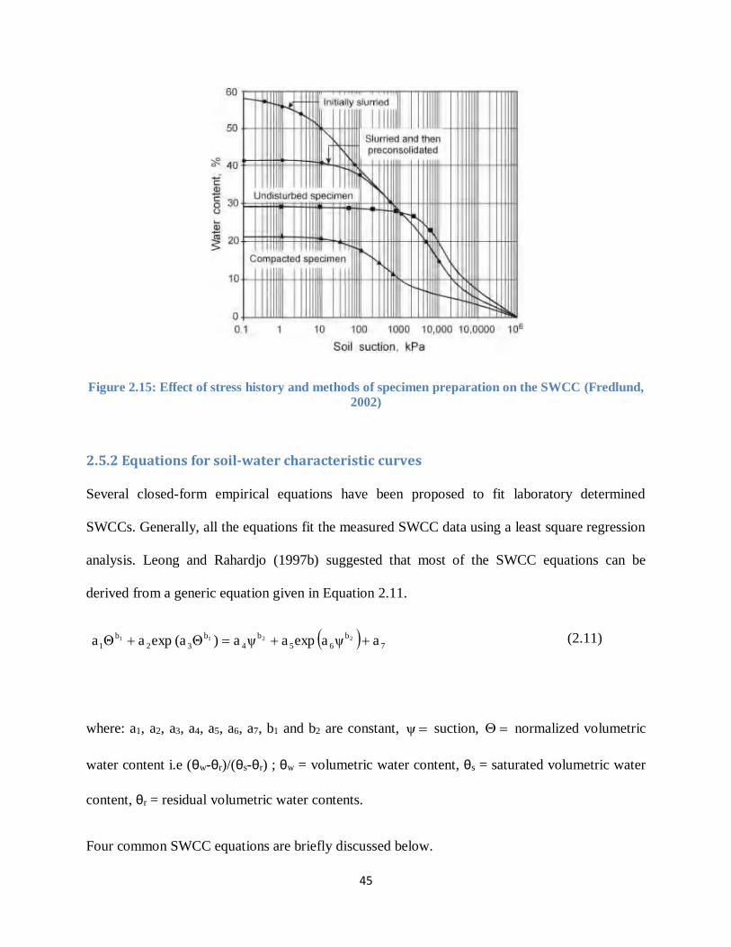
45

Figure 2.15: Effect of stress history and methods of specimen preparation on the SWCC (Fredlund,

2002)

2.5.2 Equations for soil-water characteristic curves

Several closed-form empirical equations have been proposed to fit laboratory determined

SWCCs. Generally, all the equations fit the measured SWCC data using a least square regression

analysis. Leong and Rahardjo (1997b) suggested that most of the SWCC equations can be

derived from a generic equation given in Equation 2.11.

7

b

65

b

4

b

32

b

1 aψa expaψa)Θ(a expaΘa 2211 (2.11)

where: a1, a2, a3, a4, a5, a6, a7, b1 and b2 are constant, ψ suction, normalized volumetric

water content i.e (θw-θr)/(θs-θr) ; θw = volumetric water content, θs = saturated volumetric water

content, θr = residual volumetric water contents.

Four common SWCC equations are briefly discussed below.

46

2.5.2.1 Gardner (1958)

Gardner (1958)’s equation is reported as the earliest of the SWCC equations. It is a continuous

equation which was originally formulated to model permeability of unsaturated soils but has

been adapted to model SWCC (Sillers et al., 2001). This equation, reproduced as Equation 2.12

has two fitting parameters: a which is related to the inverse of AEV and n which is related to the

pore size distribution (Gardner, 1958).

n

rs

rwaψ1

θθθθ

(2.12)

2.5.2.2 Brooks and Corey (1964)

Brooks and Corey (1964)’s equation reproduced as Equation 2.13, assumes a constant water

content for suctions less than AEV. Beyond the AEV, the material desaturates exponentially. The

equation has two fitting parameters: a which is related to the AEV and λ which is related to the

pore size distribution and is referred to as the pore size distribution index.

aψfor a

ψθ θ

aψfor θθ

λ

sw

sw

(2.13)

The larger the value of λ, the more uniform the pore size distribution is, which implies a steeper

SWCC in the transition zone (Sillers et al., 2001). One criticism for the Brooks and Corey

(1964)’s equation is its inability to provide a continuous function for the SWCC. Sillers et al.

(2001) note that the discontinuity in the function at the suction value equal to a may cause

instability during numerical modeling of unsaturated soil behavior. The Brooks and Corey

(1964) equation is more suitable for coarse-grained soils.

47

2.5.2.3 van Genuchten (1980)

van Genuchten (1980) proposed a closed-form, smooth, three-parameter SWCC equation

reproduced in Equation 2.14.

m

nrsrwαψ1

1θθθθ (2.14)

where; mn, , are fitting parameters.

van Genuchten (1980)’s equation herein referred to as VG model, allows for greater flexibility

than the previous models hence successfully fits SWCC data for a wide range of soils. The fitting

parameters have physical meaning; -1kPa α is related to the inverse of the AEV, n is related to

the pore size distribution of the soil and m is related to the overall symmetry of the SWCC

(Sillers et al., 2001).

The parameter, m is very often constrained as either; n

11m or

2n

11m which reduces the

flexibility of the model but significantly simplifies it (Lu and Likos, 2004).

In this thesis, whenever the VG model has been used, it has been regarded as four-parameter

model with residual volumetric water content θr also regarded as a fitting parameter as suggested

by Leong and Rahardjo (1997b) and the constraint on parameter m has been considered as;

n

11m .

2.5.2.4 Fredlund and Xing (1994)

Fredlund and Xing (1994) suggest a continuous, closed-form three-parameter model similar to

the VG model shown in Equation 2.15. In this thesis, the model will be referred to as FX model.

48

m

nw

a

ψeln

1ψCθ (2.15)

where C is a correction factor that ensures the SWCC goes to suction of 1GPa at zero water

content, a is a fitting parameter associated with the AEV, n is a fitting parameter associated with

the rate of desaturation of the soil past the AEV, m is a fitting parameter associated with the

residual water content, and e is natural number i.e., 2.71828..

The correction factor C as suggested by Fredlund and Xing (1994) is given in Equation 2.16

r

6

r

ψ

101ln

ψ

ψ1ln

1ψC (2.16)

where rψ = residual suction.

Leong and Rahardjo (1997b) found best fits were obtained with the FX model were obtained

when the correction factor, ψC is set to unity i.e 1 and this has been adopted in this thesis.

Further Leong and Rahardjo (1997b) found that the FX model gave the best fit to the SWCC data

of a wide range of soils compared to the other models studied. Another noted advantage of the

FX model is the ability to converge much faster compared to the VG model (Leong and

Rahardjo, 1997b; Sillers et al., 2001).

49

2.6 Permeability

Darcy (1856) was the first to quantify flow of water through porous media. Having measured

flow rates of water through saturated sand filters, Darcy (1856), discovered that the volume rate

of flow, Q is directly proportional to the cross section area, A, of the porous medium and the

hydraulic head difference between the inlet and outlet of water, Δhw, and inversely proportional

to the length, L, of the medium. This relationship is summarized in Equation 2.17.

L

A wh

Q

(2.17)

The term Δhw/L in Equation 2.17 is referred to as the hydraulic gradient (i) which is responsible

for driving the flow i.e., the driving potential. If the volume flow rate were considered per unit

cross sectional area, A, per unit time, t, and the proportionality constant, k, introduced, the flux,

q, can be computed as shown in Equation 2.18

L

Δhk

At

Qq w (2.18)

The proportionality constant, k, is referred to as the permeability or the hydraulic conductivity of

the material.

2.6.1 Saturated permeability

As noted from Darcy’s work, the driving potential for flow through saturated soils is the

hydraulic gradient i i.e., whenever there is a hydraulic gradient, flow will occur. Saturated soils

have their void filled with water and as a result their permeabilities are considered constant

(Marshall et al., 1996). Several empirical formulations have been suggested relating saturated

permeability of soils to different soil properties. Explicitly or implicitly, these formulations relate

50

saturated permeability to the void ratio, grain size characteristics and some other soil properties

such as soil structure, .

Milan and Andjelko (1992) generalized the empirical formulations for saturated permeability, k,

of soils as given in Equation 2.19.

e.dn.C.f ν

gk (2.19)

where g is acceleration due to gravity, ν is kinematic viscosity, C is sorting coefficient, f(n) is a

function of porosity, de is effective grain diameter, ν is dynamic viscosity (μ)/fluid density (ρ).

Some of the commonest empirical formulations for permeability are:

Hazen (1892)

Hazen (1892) suggested an empirical relationship predicting permeability, k (cm/s), of saturated

sands. Following the generalization form given in Equation 2.19, Hazen’s formulation is

presented in Equation 2.20.

2

10

4- .D0.26n10110.6ν

gk (2.20)

Hazen’s formulation is commonly presented simply as shown in Equation 2.21

2

10H .DCk (2.21)

where: CH = Hazen’s empirical coefficient and D10= particle size for which 10% of the soil is

finer.

51

Although Hazen developed the formulation for sands (0.01cm<D10<0.3cm), it has been widely

applied to in situ soils as well other soils which are not sands. Because of this, Carrier III (2003)

notes that Hazen’s empirical coefficient, CH ranges from 1 to 1000 according to published data

despite the fact that the coefficient usually takes on a value of 100. Hazen’s formulation

represents average situations and should be carefully applied to soils outside the range Hazen

studied (Taylor (1948).

Terzaghi (1925)

Terzaghi (1925) suggested a formulation for saturated soils given in Equation 2.22.

2

10

2

3t D.n1

0.13n.C

ν

gk

(2.22)

where Ct= sorting coefficient; 61x10-3<Ct<107x10-3

Terzaghi’s formulaltion is suited for large-grained sands (Cheng and Chen, 2007). Odong (2007)

studied permeabilities of unconsolidated aquifer materials, comparing different empirical

formulations based on grain size and concluded that Terzaghi (2007) grossly underestimated the

permeabilities and recommended that the formulation be restricted to large grain sands.

Kozeny-Carman

The Kozeny-Carman (K-C) equation was first suggested by Kozeny (1927) and later modified by

Carman (1956). The K-C equation is one of the most widely accepted empirical formulation for

estimating permeability of saturated soils (Chapuis and Aubertin, 2003; Odong, 2007; Chapuis,

2012). Although there are several forms of the K-C equation, it can be generalized as shown in

Equation 2.23

52

3-3 2

102

g nk .8 10 .D

ν 1 n

(2.23)

While most literature states that the K-C equation is best suited for sands, Chapuis and Aubertin

(2003) demonstrates that the equation can in fact be applied in predicting fairly accurately, the

saturated permeability of a wide range of soils.

2.6.2Unsaturated permeability

Despite contentions that previously surrounded the driving potential of flow in unsaturated soils,

Fredlund et al. (2012) has demonstrated that hydraulic gradient is the only driving potential for

flow in unsaturated soils similar to saturated soils.

Since the pore space in unsaturated soils consists of air and water phases, the permeability of

unsaturated soils is not only a function of void ratio but also the quantity of water in the pore

space (Fredlund and Rahardjo,1993). Therefore, since the quantity of water will vary, the

permeability of unsaturated soils is not constant but rather a function of water content or suction

of the soil. Although the permeability of unsaturated soils is not a constant, Darcy’s law can still

be applied to flow in unsaturated soils (Buckingham, 1907; Richards, 1931; Childs and Collis-

George, 1950).

2.6.2.1 Relationship between unsaturated permeability and volume-mass relations of soils

LLoret and Alonso (1980) and Fredlund (1981) state that the coefficient of permeability, kw is a

function of any two of three volume-mass properties:

kw = kw (S,e)

kw = kw (e, w)

53

kw = kw (w, S)

where: S= degree of saturation, e = void ration and w = gravimetric water content.

For unsaturated soils, the coefficient of permeability is affected by combined of changes of void

ratio and degree of saturation or water content (Fredlund et al., 2012). Some examples of

relationships between permeability, void ratio and degree of saturation of unsaturated soils are

listed in Table 2.3.

2.6.2.2 Permeability functions

Owing to the difficulties in direct measurement of unsaturated permeability such as cost,

duration of tests, and experimental difficulties (Leong and Rahardjo, 1997a; Fredlund et al.,

2012), indirect methods have been found useful. The indirect methods estimate permeability

functions by either directly or indirectly relating to the features of the SWCC (Fredlund et al.,

2012).

Leong and Rahardjo (1997a) categorise models for estimating permeability functions in indirect

methods into three in order of increasing rigor: empirical, macroscopic and statistical models.

54

Table 2.3 Relationships of unsaturated permeability with void ratio and degree of saturation

Reference Formulation Notes

Mitchell et al. (1966) 3

3

w Se1

eCk

C = constant, e = void ratio, S= degree

of saturation.

LLoret and Alonso (1980) 01 eeC

0sw 10eS,kk

C1=constant, ks=saturated permeability,

e0= initial void ratio

Chang (1976), Chang and

Duncan (1983)

m

e3

0

0

3

sw Se1e

e1ekk

Se=effective degree of saturation,

m=flexible constant

a) Empirical models

Leong and Rahardjo (1997a) present a detailed review of empirical models. Fredlund et al.

(2012) note that empirical models are constructed by recognizing the relationship between the

SWCC and the permeability function. These models therefore take on a similar shape as the

SWCC. Leong and Rahardjo (1997a) generalized most empirical models in the literature in the

form shown in Equation 2.24.

prk (2.24)

where: kr = relative permeability given as ratio of water permeability (kw) to the saturated

permeability (ks), Θ = normalized volumetric water content = (θw-θr)/(θs-θr) where the subscripts

r and s refer to residual and saturated state water contents, respectively.

55

Considering Equation 2.23, if the normalized volumetric water content, Θ, is expressed as

function of matric suction, typical of the SWCC, then the kr can directly be related to matric

suction as demonstrated by Leong and Rahardjo (1997a). The successful usage of the empirical

models requires sufficient permeability measurements so that fitting parameters are easily

optimized (Leong and Rahardjo, 1997a).

b) Macroscopic models

Macroscopic models aim at constructing analytical permeability functions (Mualem, 1986).

Mualem (1986) enlists the underlying assumptions for these models. The primary assumption is

the similarity between laminar flow at microscopic level and the macroscopic flow through a

porous media (soil). With this assumption, flow is then modeled as simple laminar flow system,

interrelating macroscopic variables such as average flow velocity, hydraulic gradient,

permeability and hydraulic radius (Mualem, 1986; Leong and Rahardjo, 1997a). With a direct

analogy made between these macroscopic variables and the corresponding variables in the soil-

water-air system, together with simplifying assumptions, Leong and Rahardjo (1997a)

generalized macroscopic models using a power function form given in Equation 2.25

δ

er Sk (2.25)

where Se = effective degree of saturation and δ = constant which varies with different

researchers.

According to Mualem (1986), the macroscopic models have a theoretical basis unlike empirical

models, are easy to use and do not require many experimental data points for calibration.

However, Childs and Collis-George (1950) note that these models neglect pore size distribution.

56

c) Statistical models

According to Mualem (1986), statistical models aim at deriving the coefficient of permeability

from the SWCC. The assumptions underlying the statistical models are (Mualem (1986):

- The porous medium is regarded as a set of interconnected pores, randomly distributed in

the sample. The characteristics of the pores are described by a statistical function, f(r).

- The Hagen-Poiseuille equation is considered valid at the microscopic level i.e., at the unit

pore level.

- The SWCC is considered analogous to the pore-size distribution function

Three statistical models are reviewed below.

Childs and Collis-George (1950) proposed a statistical model based on a random variation of

pore sizes. This model was improved by Marshall (1958) and finally modified by Kunze et al.

(1968). This model was generalized by Agus et al. (2003) as given by Equation 2.26

z

θ

0

y

w

θ

0

y

w

x

wrs

w

dξψ

ξθ

dξψ

ξθ

Θθk

(2.26)

where: Θ= normalized volumetric water content, ψ = suction, ξ = dummy variable

For the original model suggested by Childs and Collis-George (1950),x =0, y=2, and z=1 in

Equation 2.26.Agus et al. (2003) observed that the model gives better estimates for permeability

functions of clays and sands when x = 0, y = 0, and z = 2 compared to the original model.

57

Burdine (1953) proposed another statistical model that takes into account tortuosity given in

Equation 2.27.

s

w

θ

0

2

w

θ

0

2

w

2

wr

ψ

dθ

ψ

dθ

Θθk (2.27)

Mualem (1976) modified Childs and Collis-George (1950)’s model giving Equation 2.28.

2

θ

0

θ

00.5

wrs

w

ψ

ψΘθk

w

w

d

d

(2.28)

Agus et al. (2003) generalized Equations 2.27 and 2.28 into Equation 2.29

z

θ

0

y

θ

0

y

x

wrs

w

ψ

ψΘθk

w

w

d

d

(2.29)

According to Fredlund and Rahardjo (1993), the computation procedures are implemented by

dividing the SWCC into several equal increments of volumetric water contents as illustrated in

Figure 2.16. The relative permeability kri at specific volumetric water content θwi is then

computed by summing suctions corresponding to volumetric water contents at and below the

specific volumetric water content.

The permeability function is calculated using Equation 2.30 which is a modification of Kunze et

al. (1968)’s equation with pressure head replaced with matric suction (ua – uw) (Fredlund and

Rahardjo, 1993)

58

Figure 2.16: Calculation of the permeability function from the SWCC (from Marshall, 1958; Kunze

et al, 1968 )

m

ij

2

jwasiw uu2i12jkθk (2.30)

where: iθk w = calculated coefficient of permeability for a specified volumetric water content,

iθ corresponding to the ith interval, ks = measured saturated permeability, i = interval number

that increases with decreasing water content, and j = counter from i to m.

2.6.3 Laboratory measurement of permeability

2.6.3.1 Saturated permeability

Two methods are usually used to measure saturated permeability in the laboratory i.e., the

constant head and falling head techniques. In the constant head method, the hydraulic gradient is

maintained constant in the test and the inflow or outflow volume rate of water is measured. The

saturated permeability, ks, is then measured according to Darcy’s law using Equation 2.31

59

s

w

QLk

Δh At (2.31)

where: Q = inflow/outflow rate of volume flow, L = length of soil specimen, Δhw = hydraulic

head difference, A = cross section area of the soil specimen, and t = time.

In the falling head method, the hydraulic gradient changes with time but the principle of

continuity of flow is observed. Therefore ks is computed using Darcy’s law with Equation 2.32.

1s

2

aL hk ln

At h

(2.32)

where a = cross section area of the water reservoir, A = cross section area of the soil specimen, L

= length of soil specimen, h1 = hydraulic head at time t1, h2 = hydraulic head at time t2, and t =

time

These techniques can be applied to both the flexible and rigid wall permeameters that are

commonly used to measure permeability in the laboratory. These techniques have been

standardized in ASTM D5084-16a which details the procedure for measuring saturated

permeability of soils using the flexible wall permeameter and ASTM D5856-15 which details the

procedure to follow for the rigid wall permeameter.

The rigid wall permeameter, also called a fixed wall or a compaction mould permeameter

(ASTM D5856-15), is largely used on compacted soils. Daniel et al. (1985) notes that the fixed

wall permeameter is an affordable equipment however very often experiences side-wall leakage

which leads to over estimation of permeability. In the same work, Daniel et al. (1985) describes

the different modifications of the fixed wall permeameter together with their applicability,

advantages and disadvantages. The flexible-wall permeameter is usually constructed out of a

60

triaxial or modified triaxial system (Daniel et al., 1984, Daniel et al., 1985). Although more

costly and complicated to construct, the flexible-wall permeameter has numerous advantages

over the fixed-wall permeameter. According to Daniel et al. (1985), the flexible wall

permeameter is best suited for soils with irregular sides (such as natural soils, compacted soils

with large particle sizes and clods), has no problem of side-wall leakage, saturation of samples

can be enhanced by application of back pressure, permeability studies can be conducted at

desired effective stress level and unsaturated permeability can easily be associated with the stress

state variables (Samingan et al., 2003). Owing to its advantages, this study used the flexible-wall

permeameter to determine the saturated permeability of the compacted soil.

2.6.3.2 Unsaturated permeability

Unsaturated permeability can be determined directly in the laboratory using either steady or

unsteady methods. Measuring the unsaturated permeability of a soil requires a HAEV ceramic

disk to separate the air and water phases. In order to minimize head loss across the HAEV disk,

ASTM D7664-10 recommends the saturated permeability of the HAEV ceramic disk must be at

least two orders of magnitude higher than the saturated permeability of the soil specimen to be

measured.

One disadvantage of steady methods is that they require long duration and accurate volume

determination (Klute, 1965; Klute, 1972; Olson and Daniel, 1981). Examples of equipment that

have been designed to measure unsaturated permeability using steady state methods include:

Klute (1965), Barden and Pavlakis (1971), and Huang et al. (1998).

Unsteady-state methods are attractive because they take a shorter time to conduct. These

methods include instantaneous profile method (Richards and Weeks, 1953; Meerdink et al.,

61

1996; Krisdani et al., 2009), single or multi step outflow method (Gardner, 1956; Šimůnek et al.,

1998; To-Viet et al., 2013), absorption method (Bruce and Klute, 1956) and sorptivity (Klute and

Dirksen, 1986). However, the analysis to obtain the unsaturated permeability is more complex

and both pore-water pressure and water content measurements are required.

2.6.4 Field measurements of permeability in the vadose zone

For laboratory techniques to be gainful, the samples must be carefully selected so that field

conditions are represented as closely as possible. This may be quite difficult especially for

coarse-grained soils. Secondly, in order to cater for the spatial variability, a large scale sampling

exercise must be done which is very often hindered by resources. Due to these setbacks, field

tests can be very useful and more representative. Some examples of field permeability tests in the

vadose zone are briefly discussed below.

2.6.4.1 Constant head well permeameter

The constant head well permeameter sometimes referred to as a borehole permeameter is used to

measure field-saturated permeameter. The permeability is measured around a well, augered in

the unsaturated zone (Reynolds and Elrick, 2002). In addition to permeability, other

measurements can be obtained such as matric flux potential, macroscopic capillary length

parameter and the wetting front pressure head (Reynolds and Elrick, 2002).This method is based

on a three dimensional quasi-steady state flow analysis.

According to Reynolds and Elrick (2002), the test may be carried out at a single or multiple

heads i.e., the borehole may be ponded at different heads in order to establish the desired

hydraulic parameters.

62

Several designs of the permeameter exist. Figure 2.17a shows an example of a schematic of the

constant head well permeameter. Figure 2.17b shows the schematic diagram of the borehole

simulating the flow domain. In order to minimize the effects of smearing, a sharp auger is used,

augering is not done in wet soils especially clays and excess pressure on the auger is avoided.

Smearing of the borehole influences the infiltration characteristics hence affecting the measured

permeability (Reynolds and Elrick, 2002).

The permeameter is set up in the borehole and stabilized using a tripod stand as shown in Figure

2.17. Backfill material is necessary to avoid collapse of the borehole during testing when dealing

with collapsible ground. In addition, Reynolds and Elrick (2002), notes that backfill material can

minimize siltation of the well and ensures faster and uniform bubbling of the air tube especially

when dealing with low permeability materials. Once the permeameter is filled with water, the air

tube is lifted in order to attain the target head, H, in the borehole. The discharge, Q, is monitored

until it attains a steady state. Elrick and Reynolds (1992) proposed a formula to estimate field

saturated permeability, Ks for a steady state discharge, Qs under a single steady state head, given

in Equation 2.33.

63

a) b)

Figure 2.17: Schematic representation of a) the constant head well permeameter(Reynolds and

Elrick, 2002), and b) the simulation domain(Hayashi and Quinton, 2004)

1

22

ss πaαC

2ππ

C

2ππQK

(2.33)

where H = steady state depth of water in the well, C= dimensionless shape factor, α=parameter

associated with effects of capillarity under steady state conditions, and a = radius of the well.

The underlying assumptions when applying this technique are: the soil is homogenous, isotropic

and wetting of the soil is uniform

In order to minimize the boundary influence, Reynolds and Elrick (1987) suggested that

boundaries should be located at a distance of at least 10H. Reynolds and Elrick (2002) presents

formulations for estimating hydraulic parameters of the soil using multiple heads.

Daniel (1989) notes that the method is relatively affordable, easy to install, quite fast and takes

into consideration unsaturated behavior. However, the method essentially measures horizontal

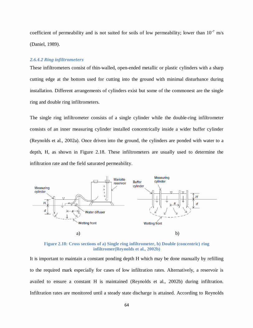
64

coefficient of permeability and is not suited for soils of low permeability; lower than 10-7 m/s

(Daniel, 1989).

2.6.4.2 Ring infiltrometers

These infiltrometers consist of thin-walled, open-ended metallic or plastic cylinders with a sharp

cutting edge at the bottom used for cutting into the ground with minimal disturbance during

installation. Different arrangements of cylinders exist but some of the commonest are the single

ring and double ring infiltrometers.

The single ring infiltrometer consists of a single cylinder while the double-ring infiltrometer

consists of an inner measuring cylinder installed concentrically inside a wider buffer cylinder

(Reynolds et al., 2002a). Once driven into the ground, the cylinders are ponded with water to a

depth, H, as shown in Figure 2.18. These infiltrometers are usually used to determine the

infiltration rate and the field saturated permeability.

a) b)

Figure 2.18: Cross sections of a) Single ring infiltrometer, b) Double (concentric) ring

infiltromer(Reynolds et al., 2002b)

It is important to maintain a constant ponding depth H which may be done manually by refilling

to the required mark especially for cases of low infiltration rates. Alternatively, a reservoir is

availed to ensure a constant H is maintained (Reynolds et al., 2002b) during infiltration.

Infiltration rates are monitored until a steady state discharge is attained. According to Reynolds

65

et al. (2002b), the time required to attain steady state conditions depends on the soil texture, soil

structure, depth of ponding (H), depth of embedment of the cylinders (d) and the radius of the

cylinders (a)

Elrick and Reynolds (1990) suggested a formulation for computing the field saturated hydraulic

conductivity, Ks from a ring infiltrometer at quasi-steady state conditions given in Equation 2.34

1a)Cdα(C

1

aCdC

Hπa

Q

K

2121

2s

s

(2.34)

where Qs= steady state discharge, a= radius of the ring, H= steady state depth of ponded water in

the ring, d= depth of ring embedded into the ground, α= macroscopic capillarity length while C1

and C2 are dimensionless constants.

Ring infiltrometers have great advantages for example affordability, ease of installation, capacity

to give good estimate of vertical hydraulic conductivity due to the rings that restrict lateral

spread. Despite these advantages, this technique has some major setbacks. The need to attain

steady state infiltration may lead to long durations of time ranging from a few minutes to days

depending on the size of cylinders, soil structure and texture (Scotter et al., 1982; Daniel, 1989).

Daniel (1989) notes the need to correct for evaporative losses and difficulty to set up on a

sloping ground unless a bench is established. It is important to also note that as the cylinders are

driven into the ground, the soil may be disturbed hence influencing the subsequent

measurements.

66

2.6.4.3 Tension or disk infiltrometers

These devices are usually used to determine field near-saturation permeability and sorptivity. A

tension infiltrometer consists of an infiltrometer plate which may be a membrane or a

hydrophilic porous disk (Reynolds, 2008). The disk/membrane is connected to a water reservoir

which supplies it with water and a bubble tower that is used to control the suction head on the

disk/membrane.

When placed on an unsaturated porous medium, the capillarity in the disk/membrane draws

water out of the reservoir into the porous medium hence infiltration into the porous medium at

the set suction head (Reynolds, 2008).

Since disk infiltrometers supply only a small tension at the soil surface, the effects of macropores

on the infiltration are eliminated thus ensuring that only infiltration properties of the soil matrix

are determined (Clothier and White, 1981). According to Clothier and White (1981), macropores

have little influence during a natural rainfall infiltration and infiltration is controlled by the soil

matrix. White and Sully (1987) further note that in order to reasonably offset the influence of

macropores, the diameter of the disk should be at least equal to the macroscopic capillary length

of the soil.

Techniques of obtaining hydraulic properties of the soil from disk infiltrometers can be

categorized into steady state flow and transient flow. Wooding (1968) showed that the steady

state flow rate, Qo, of water from a surface disk of radius, r, containing water at a matric suction

head, ψo is given by Equation 2.35

2

O OQ πr k 4rψo (2.35)

67

The characteristics of transient flow from disk infiltrometers are approximated by the first two

terms of Philip (1957)’s expansion of the infiltration equation as given in Equation 2.36.

tCtCI 22

1

1 (2.36)

where I is the cumulative infiltration at a matric suction head, C1 (ms-1/2) and C2 (ms-1) are the

parameters related to soil sorptivity, S and hydraulic conductivity, K, respectively.

Haverkamp et al. (1994) suggested a solution to Equation 2.36 which relates sorptivity S and

permeability, k as given in Equation 2.37.

1

2

2

o i

C S

2 β γSC K

3 r θ θ

(2.37)

where ϒ is proportionality constant in the range 0.6 -0.8, β is a coefficient lying between 0 and 1,

r is the radius of the disk, θo is the final water content and θi is water content corresponding to

the matric suction head imposed on the disk. Parameters C1 and C2 are obtained by curve fitting

Equation 2.36 to the infiltration data. Once C1 and C2 are known, k and S can be computed.

Zhang (1997) suggested simple linear solutions to Equation 2.36 given in Equation 2.38.

hKA(h)C

hSA(h)C

22

11

(2.38)

where A1 and A2 are dimensionless coefficients and h is the pressure head at which the mini-disk

infiltrometer is set. Based on results of numerical experiments, Zhang (1997) suggested

empirical relationships for calculating A1 and A2 given in Equation 2.39 and 2.40, respectively.

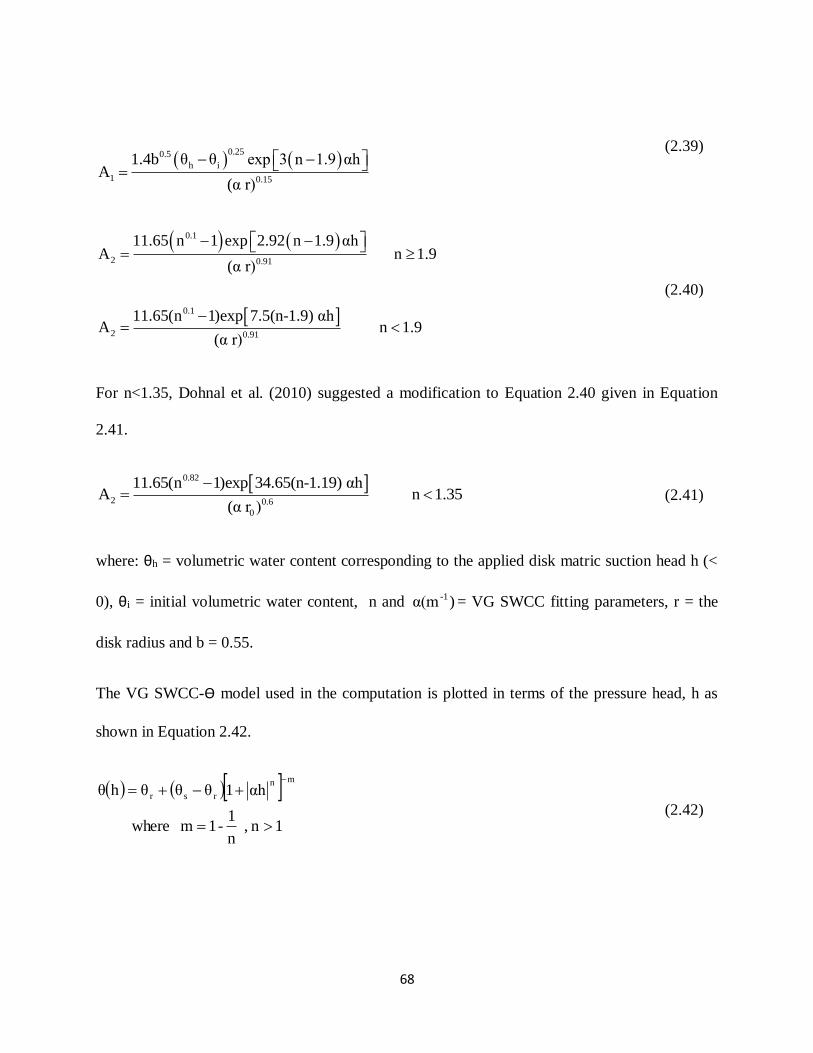
68

0.250.5

h i

1 0.15

1.4b θ θ exp 3 n 1.9 αhA

(α r)

(2.39)

0.1

2 0.91

0.1

2 0.91

11.65 n 1 exp 2.92 n 1.9 αhA n 1.9

(α r)

11.65(n 1)exp 7.5(n-1.9) αhA n 1.9

(α r)

(2.40)

For n<1.35, Dohnal et al. (2010) suggested a modification to Equation 2.40 given in Equation

2.41.

0.82

2 0.6

0

11.65(n 1)exp 34.65(n-1.19) αhA n 1.35

(α r )

(2.41)

where: θh = volumetric water content corresponding to the applied disk matric suction head h (<

0), θi = initial volumetric water content, n and )α(m -1 = VG SWCC fitting parameters, r = the

disk radius and b = 0.55.

The VG SWCC-Ѳ model used in the computation is plotted in terms of the pressure head, h as

shown in Equation 2.42.

1n ,

n

1-1m ere wh

αh1θθθhθmn

rsr

(2.42)

69

Carsel and Parrish (1988) conducted several water retention experiments on different soil

textural classes and developed average values for VG model parameters; n, α, θs and θr. Table 2.4

summarizes the findings of Carsel and Parrish (1988).

The n and α in Table 2.4 are very often used to solve Equation 2.40. This makes determination of

the permeability very fast especially in the absence of time and facilities to measure the SWCC

of the soil. However, it is important to check how reliable the permeability measurements

obtained using Table 2.4 are compared to those obtained using the actual SWCC. This aspect

was investigated in this thesis.

A mini-disk infiltrometer which is used in this study is one type of tension infiltrometer. Extra

advantages of the mini-disk infiltrometer is its portability, ease of use, and fast measurements in

the field.

70

Table 2.4 VG model calibration parameters for 12 soils (Carsel and Parrish, 1988)

Textural class α (cm-1) n θs θr

Sand 0.145 2.68 0.43 0.045

Loamy sand 0.124 2.28 0.41 0.057

Sandy Loamy 0.075 1.89 0.41 0.065

Loam 0.036 1.56 0.43 0.078

Silt 0.016 1.37 0.46 0.034

Silt Loam 0.020 1.41 0.45 0.067

Sandy Clay Loam 0.059 1.48 0.39 0.100

Clay Loam 0.019 1.31 0.41 0.095

Silty Clay Loam 0.010 1.23 0.43 0.089

Sandy Clay 0.027 1.23 0.38 0.100

Silty Clay 0.005 1.09 0.36 0.07

Clay 0.008 1.09 0.38 0.068

2.7 Shear strength of unsaturated soils

Shear strength behaviour of unsaturated soils is of great concern in engineering practice because

unsaturated soils are very often encountered in practice. Over the years, the research community

has contributed enormously towards understanding shear strength behavior of unsaturated soils.

71

Despite this effort, adoption by practitioners remains low owing to several factors some of which

include: complexity of the science, expensive equipment, and test duration. Yet, unsaturated soil

mechanics is needed to analyse rain-induced slope failures and seepage flow through dams,

design remedial measures for failed slopes and waste containment system, and other problems in

the vadose zone. In this thesis, the aspects of interest on shear strength of unsaturated soils are

the shear strength equations and the testing procedures available. The literature review will be

restricted to these two aspects.

2.7.1 Shear strength equations of unsaturated soils

Shear strength equations for unsaturated soils are commonly categorized based on the stress state

variables criteria. Following subsection 2.3, the shear strength equations will be classified into

two major categories: (i) equations based on a single stress state variable, and (ii) equations

based on independent stress state variables.

2.7.1.1 Single stress state variable approach

a) Effective stress approach

The effective stress approach proposed by Bishop (1959) is the commonest in this category.

Bishop (1959) proposed that effective stress in an unsaturated soil can be defined by combining

two stress state variables i.e. net normal stress, (σn-ua) and matric suction, (ua-uw) in addition to

a material variable, χ . This formulation was reproduced in Equation 2.1.

One noted advantage of the effective stress approach is that it follows directly from the classical

soil mechanics formalism of effective stress approach and is usually applied with the

conventional Mohr-Coloumb (M-C) failure criterion. Therefore Equation 2.1, substituted into the

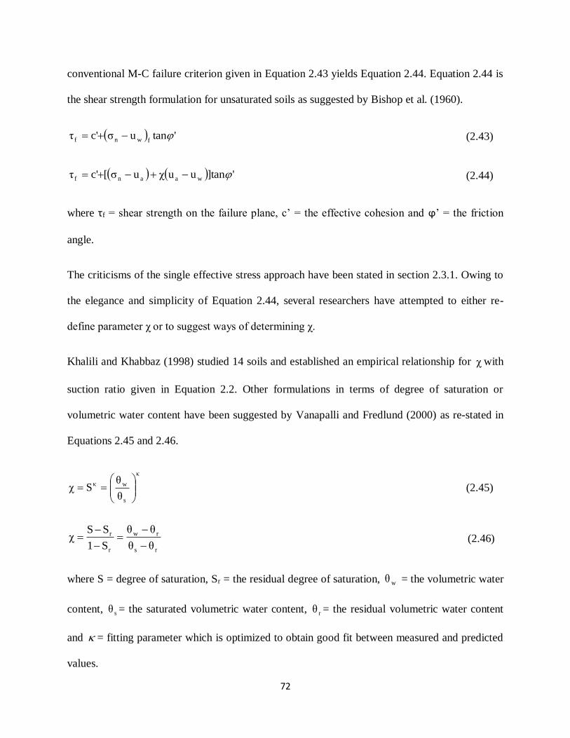
72

conventional M-C failure criterion given in Equation 2.43 yields Equation 2.44. Equation 2.44 is

the shear strength formulation for unsaturated soils as suggested by Bishop et al. (1960).

'tanuσc'τfwnf (2.43)

']tanuuχuσ[c'τ waanf (2.44)

where τf = shear strength on the failure plane, c’ = the effective cohesion and ϕ’ = the friction

angle.

The criticisms of the single effective stress approach have been stated in section 2.3.1. Owing to

the elegance and simplicity of Equation 2.44, several researchers have attempted to either re-

define parameter χ or to suggest ways of determining χ.

Khalili and Khabbaz (1998) studied 14 soils and established an empirical relationship for χ with

suction ratio given in Equation 2.2. Other formulations in terms of degree of saturation or

volumetric water content have been suggested by Vanapalli and Fredlund (2000) as re-stated in

Equations 2.45 and 2.46.

κ

s

wκ

θ

θSχ

(2.45)

rs

rw

r

r

θθ

θθ

S1

SSχ

(2.46)

where S = degree of saturation, Sr = the residual degree of saturation, wθ = the volumetric water

content, sθ = the saturated volumetric water content, rθ = the residual volumetric water content

and = fitting parameter which is optimized to obtain good fit between measured and predicted

values.

73

Following Bishop (1959)’s formulation, other researchers have suggested shear strength

equations based on a single stress variable. Three common ones are presented below:

a. Greacen (1960)

Greacen (1960) proposed Equation 2.47.

awanf n1'tanuuστ (2.47)

where na is the fraction of the voids filled with air.

Equation 2.47 assumes that suction in the soil water for an unsaturated soil supplies an additional

isotropic stress on the internal area of contact hence increasing the soil’s potential to resist shear.

This implies that that increase in strength of an unsaturated soil is proportional to both an

increment in applied normal stress and matric suction present in the soil again implying a single

stress variable as suggested by Bishop (1959). Therefore, the limitations in Equation 2.44 also

apply to Equation 2.47.

b. Lamborn (1986)

Extending micromechanics model by applying the principle of irreversible thermodynamics to a

composite volume, Lamborn (1986) suggested Equation 2.48 to evaluate shear strength of

unsaturated soils.

'tanθuu'tanuσc'τ wwaanf (2.48)

where: θw= volumetric water content.

Equation 2.48 is based on a single stress state variable in which shear strength in an unsaturated

soil varies with the volumetric water content. According to Vanapalli (1994), this is only logical

74

if the desaturation process can be linked to the contribution that volumetric water content makes

on shear strength.

c. Öberg and Sällfors (1997)

Öberg and Sällfors (1997) proposed Equation 2.49 to predict shear strength of unsaturated silts

and sands based on the SWCC.

'tan1c'τ f aw uSSu (2.49)

where S = degree of saturation.

As determining to degree of saturation through the fraction of pore that are occupied by water

i.e. tot

w

A

A. Therefore if the soil’s SWCC is established, the shear strength of the soil can be

determined for various degrees of saturation if the internal friction angle, ' is known.

Despite the fact that there is no unique relationship between

tot

w

A

A and S, Equation 2.49

has been found to give satisfactory results in engineering practice (Öberg and Sällfors, 1997).

Vanapalli and Fredlund (2000) found that Equation 2.49 did not give good predictions of shear

strength in relation to measured data irrespective of the suction range. However, Vanapalli and

Fredlund (2000) tested the equation only on clayey material which may have affected its

performance.

75

2.7.1.2 The independent stress state variable approach

Fredlund et al. (1978) proposed the concept of two independent stress state variables using

multiphase continuum mechanics. This theory extends the Mohr-Coloumb failure envelope to a

3D planar surface. The formulation is re-stated in Equation 2.50

b

f n a a wf fτ c' σ u tan ' u u tan (2.50)

where c’ = the effective cohesion on the failure plane, (σn-ua)f = the net normal stress at the

failure on the failure plane at failure, (ua-uw)f = matric suction on the failure plane at failure, ’ =

internal friction angle associated with the net normal stress (σn-ua)f, and ϕb = angle indicating the

rate of increase of shear strength with matric suction, (ua-uw).

Figure 2.19 illustrates the planar surface generated using Equation 2.50. The Mohr-circles are

constructed in the 3-D space.

Equation 2.50 can be re-written as

f a fτ C σ u tan 'n (2.51)

where:

b

a wC c' u u tan (2.52)

Equation 2.52 is the equation of line of intercept of the extended M-C envelope with the matric

suction axis as shown in Figure 2.19.

With Equation 2.51, the extended M-C envelope can be reduced to a 2-D τ-(σ-ua) plot in which

the intercept on the τ axis is C as given in Equation 2.52.In this case, C is referred to as the total

cohesion. Lu and Likos (2004) define the term b

a wu u tan as capillary cohesion, c’’.

76

While Fredlund et al. (1978) assumed a constant value of b for the entire range of soil matric

range, later studies have demonstrated that b varies with suction.

Figure 2.19: Extended Mohr-Coulomb failure envelope (from Fredlund and Rahardjo, 1993)

Shen and Yu (1996) proposed two hyperbolic equations for describing the shear strength of

unsaturated soils shown in Equations 2.53 and 2.54.

'tanduu1

1uu'tanuσc'τ

wa

waanf

(2.53)

'tan

β

uucotα

1uu'tanuσc'τ

1

wa

waanf

(2.54)

where: d = fitting parameter, α= initial angle of shear strength with respect to shear strength, and

77

β= matric suction contribution to shear strength at peak value of shear strength.

Vanapalli et al. (1996a) proposed two formulations to capture the non-linearity of the extended

M-C shear strength envelope shown as Equations 2.55 and 2.56.

'tanSuu'tanuσc'τfwafanf (2.55)

'tanS-1

S-Suu'tanuσc'τ

r

r

fwafanf (2.56)

where S = degree of saturation, Sr = residual degree of saturation, and = fitting parameter.

The formulations in Equations 15 and 16 can also be expressed in terms of volumetric or

gravimetric water contents.

Garven and Vanapalli (2006b) found that the fitting parameter is closely related to the

plasticity index, PI, of the soil as shown in Equation 2.57.

10.0975PI0.0016PIκ 2 (2.57)

One advantage of formulations in Equations 2.55 and 2.56 is the ease of use with a SWCC of the

soil. According to Garven and Vanapalli (2006a), commonly used shear strength equations

consist of two parts: one part is the shear strength of the soil under saturated condition and the

other part is the contribution to shear strength by the matric suction as shown by Equation 2.58.

msat τττ (2.58)

where: τ = total shear strength, satτ = shear strength of the soil under saturated conditions and mτ

= contribution to shear strength of matric suction. This observation can clearly be associated to

78

all the formulations presented above. Further Equation 2.58 can be further expressed as shown in

Equation 2.59

waan uu'αtan'tanuσc'τ (2.59)

where α is a function that varies depending on the formulation, τsat = c’+(σn-ua)tanϕ’ and τm =

α(ua-uw) tanϕ’.

Equation 2.59 can be closely linked to Equation 2.44 and with such an attempt, the parameter, α

can be severally defined. This has been demonstrated by Leong (2019) and partly shown in Table

2.5.

What is clear from Table 2.5 is the non-unique definition of χ as stated by different researchers.

However, Table 2.5 also reveals an endeavour to reconcile the different shear strength equations

and a successful reconciliation will greatly enhance application of unsaturated soil mechanics in

practice.

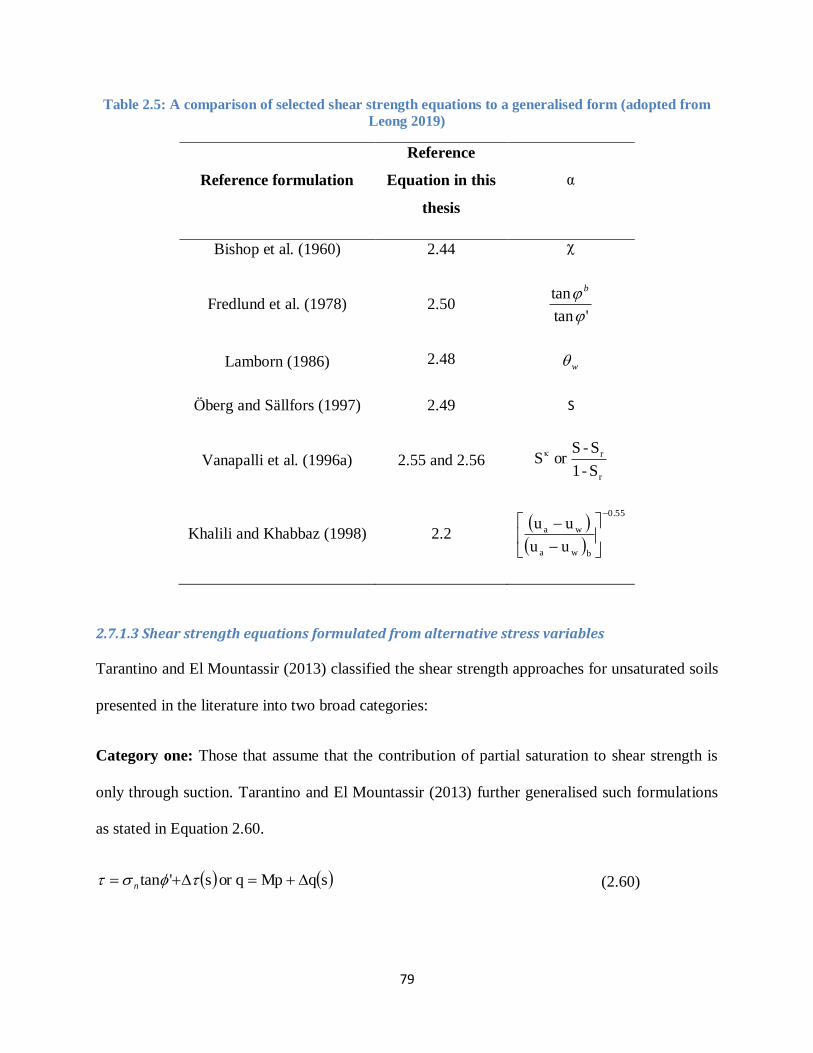
79

Table 2.5: A comparison of selected shear strength equations to a generalised form (adopted from

Leong 2019)

Reference formulation

Reference

Equation in this

thesis

α

Bishop et al. (1960) 2.44 χ

Fredlund et al. (1978) 2.50 'tan

tan

b

Lamborn (1986) 2.48 w

Öberg and Sällfors (1997) 2.49 S

Vanapalli et al. (1996a) 2.55 and 2.56 r

rκ

S-1

S-Sor S

Khalili and Khabbaz (1998) 2.2

0.55

bwa

wa

uu

uu

2.7.1.3 Shear strength equations formulated from alternative stress variables

Tarantino and El Mountassir (2013) classified the shear strength approaches for unsaturated soils

presented in the literature into two broad categories:

Category one: Those that assume that the contribution of partial saturation to shear strength is

only through suction. Tarantino and El Mountassir (2013) further generalised such formulations

as stated in Equation 2.60.

sqMpqor s'tan n (2.60)

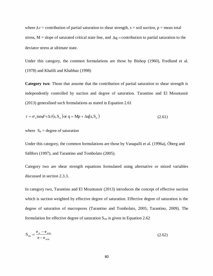
80

where = contribution of partial saturation to shear strength, s = soil suction, p = mean total

stress, M = slope of saturated critical state line, and Δq contribution to partial saturation to the

deviator stress at ultimate state.

Under this category, the common formulations are those by Bishop (1960), Fredlund et al.

(1978) and Khalili and Khabbaz (1998)

Category two: Those that assume that the contribution of partial saturation to shear strength is

independently controlled by suction and degree of saturation. Tarantino and El Mountassir

(2013) generalised such formulations as stated in Equation 2.61

Ss,qMpqor Ss,'tan n (2.61)

where Sα = degree of saturation

Under this category, the common formulations are those by Vanapalli et al. (1996a), Öberg and

Sällfors (1997), and Tarantino and Tombolato (2005).

Category two are shear strength equations formulated using alternative or mixed variables

discussed in section 2.3.3.

In category two, Tarantino and El Mountassir (2013) introduces the concept of effective suction

which is suction weighted by effective degree of saturation. Effective degree of saturation is the

degree of saturation of macropores (Tarantino and Tombolato, 2005; Tarantino, 2009). The

formulation for effective degree of saturation Srm is given in Equation 2.62

wm

wmw

rmee

eeS

(2.62)

81

where e = void ratio, ew = water ratio i.e wGs and ewm = microstructural water ratio associated

with adsorbed water. Effective degree of saturation is used on the basis that only capillary water

contained in the macropores contributes to the shear strength of the soil.

Utilization of category two equations as stated in section 2.3.3 accounts for aspects such as void

ratio and hysteresis. Furthermore, Tarantino and El Mountassir (2013) demonstrated that this

conceptualization of shear strength can reduce the rigor of testing since it can easily be adopted

with conventional equipment in order to interpret simple tests such as the constant water content

test.

It is interesting to note overlapping of concepts for example, while Öberg and Sällfors (1997)’s

formulation given in Equation 2.49 can be idealized as an equation constructed using a single

effective stress variable, it can still be categorized as one with mixed stress variables. This is also

true for Vanapalli et al. (1996a)’s formulations. It is these agreements and controversies that

hinder the application of unsaturated soil mechanics. More research is required to reach

consensus.

2.7.2 Shear strength testing for unsaturated soils

Existing literature enlists two major tests to obtain shear strength parameters of unsaturated soils;

the consolidated drained (CD) test and the constant water content (CW) test. The CD tests

commonly reported in literature (Ho and Fredlund, 1982; Rahardjo et al., 1995; Rahardjo et al.,

2004) used the axis-translation technique (ATT) as suggested by Hilf (1956) to maintain a

constant suction during consolidation and shearing phases. In the CD test, both the air and water

phases are drain during the test. The test is performed at a slow rate to ensure no pore-water

pressure build up occurs in the specimen during shearing. The CD test has been noted to have

82

several setbacks which includes the long duration of the test, highly sophisticated and costly

equipment and ATT may not necessarily reflect the real soil behavior in nature and practice.

Thu et al. (2006), Marinho et al. (2016), de Oliveira et al. (2016), note that the CW test can

address some of the concerns of the CD test. Thu et al. (2006) and de Oliveira et al. (2016) note

that construction of engineering structures using compacted cohesive soils is best represented

using a CW test given that the soils have low permeability and the construction is usually done

very fast thus not allowing drainage of the water phase, although the air phase is usually drained

or is at atmospheric state. This is simulated in the CW test when the air phase of the soil

specimen is allowed to drain while the water phase is in an undrained state.

Traditionally, the CW test is performed using the ATT which ensures that suctions higher than

100kPa are attained. The ATT imposes a constant air pressure onto the soil specimen while

changes in pore-water pressure and soil suction are monitored (Rahardjo et al., 2004, Thu et al.,

2006, Jotisankasa et al., 2009). In all these studies, the soil specimen is pre-saturated in the

triaxial cell and consolidated at a given confining pressure. At the end of consolidation phase, the

soil specimen is allowed to equilibrate at a selected matric suction using ATT prior to shearing.

During shearing phase, the air pressure, ua, is maintained while the pore-water pressure, uw, in

the soil specimen is monitored using pore-water pressure probes.

de Oliveira et al. (2016) and Marinho et al. (2016) suggested more accessible procedures for the

CW test by eliminating the need for the ATT. In these procedures, the CW test is done on the as-

compacted soil specimens with matric suctions monitored using a high capacity tensiometer

(HCT) at the base of the specimen. The challenge with these tests was ensuring matric suction

equalization in the soil specimen. The confining pressure is applied and matric suction monitored

83

with the HCT until it becomes stable under the confining pressure. The shearing phase of the test

was done in load steps, ensuring matric suction equalization with each load step before the next

until the specimen failed. These procedures are promising in making unsaturated soil mechanics

more accessible to practicing engineers. In fact, Marinho et al. (2016), demonstrated that if a CW

test is done well and matric suctions accurately determined, there may be no practical need for

determining the conventional saturated parameters i.e., ϕ’ and c’. These can be inferred from the

3D shear strength envelope.

However some drawbacks noted are: the cost and availability of HCT, the difficulty in

saturating the HCT especially where the AEV of the ceramic disk is high, the likelihood of

cavitation of the HCT system, and the difficulty to measure shear strength of dry soils with very

high matric suctions. This study therefore attempts to measure shear strength of as-compacted

soils with varying degrees of saturation using simple conventional tests. The main aim is to

investigate the possibilities of interpreting unsaturated shear strength parameters within a short

time duration using conventional equipment.

2.8 Concluding remarks

The chapter has given a brief overview of the fundamental concepts of unsaturated soil

mechanics which are: the stress state variables, measurement and control of suction, the SWCC,

hydraulic properties, and shear strength. Enormous strides in the development of the theory and

appropriate test procedures have been noted. However, despite these strides, application of

unsaturated soil mechanics in routine engineering practice is still limited.Some of the noted

issues of interest to this thesis are:

84

1) The need to agree on stress state variables well suited for applications of unsaturated soil

mechanics is still important. Despite great contributions, the research community lacks

unanimity on this issue. This in turn affects equipment design and test protocols.

2) Suction control methods are an important part of applying unsaturated soil mechanics.

The axis translation technique which is the commonest has drawn a lot of debate in recent

years regarding its suitability in representing natural conditions.

3) Suction measurement techniques have developed over the years. The commonest ones

have been presented in the chapter. Of interest to this thesis is the filter paper and the

chilled-mirror dewpoint techniques. The advantages and drawbacks of these techniques

have been presented. However, it is the position of this thesis that these techniques be

further studied to clarify on issues like: equilibrium time, hysteresis, variability of filter

papers and practical aspects surrounding their application.

4) Great advancements have been made in the theory and measurement of the SWCC. The

SWCC as discussed in the chapter is key in implementation of unsaturated soil

mechanics. The noted challenges from literature largely are duration of testing. Also

more test data is still needed to validate the numerous models and observations that have

been made over the years. This thesis has measured SWCCs for dynamically compacted

soils and attempted to explain the different observations and where necessary validated

existing theory.

5) A lot of work has been done regarding permeability including formulation of governing

theory, measurement techniques and estimation. However there is still great need to

develop fast and reliable methods for measuring permeability. The saturated permeability

measurements in particular are an important measurement since from it permeability

85

functions for unsaturated soils can be estimated. Therefore, the thesis explores the

application of a mini-disk infiltrometer in estimating saturated permeabilities. The disk

infiltrometer is affordable, fast and therefore if found reliable, this will greatly improve

the measurement of permeability.

6) Shear strength is a key property of soils. The common practice in unsaturated soil

mechanics is to use suction-controlled tests that apply the axis translation technique. The

drawback of these tests are the long test duration, cost of equipment and high level of

expertise required. The thesis therefore attempts to explore possibility of measuring

unsaturated shear strength using simple CW tests in which conventional tests and

equipment are used. This, if found plausible will be useful in bridging saturated and

unsaturated soil mechanics.

86

Chapter 3. Research Programme

3.1 Introduction

This chapter describes the soils for the experimental programme of this research project, together

with the basic properties of the soils. The procedures used for making the soil specimens for the

subsequent experiments are also presented. Finally, the apparatus, experimental set-ups and

testing procedures employed in the research are described.

3.2 Soils and basic properties

The soils used in this research project were residual soils obtained from the Jurong Formation

(JF) and the Bukit Timah Granite (BT) of Singapore. Owing to the variability in soil properties

in the two formations (Leong et al., 2002a; Rahardjo et al., 2012), two soils at different locations

were obtained for each formation. All soils were sampled in disturbed form. The materials are

designated as BT1 and BT2 for soil materials from the Bukit Timah Granite and JF1 and JF2 for

soil materials from the Jurong Formation. The Bukit Timah Granite is mainly an acidic igneous

rock system while the Jurong Formation is predominantly a folded sedimentary rock system

(Leong et al., 2002a). The upper layers of these formations were weathered into residual soils of

varying thickness. Generally, the weathering depths in JF are greater than that in the BT. Table

3.1 shows the basic soil properties while Figure 3.1 shows the grain size distribution of the soils.

Using Equation 3.1 as suggested by Fredlund (2000), Rahardjo et al. (2012) suggested lower and

upper envelope bounds to grain size distributions (GSD) as well as typical GSDs for soils from

the three major geological formations (Jurong Formation, Bukit Timah Granite and Old

Alluvium) of Singapore.

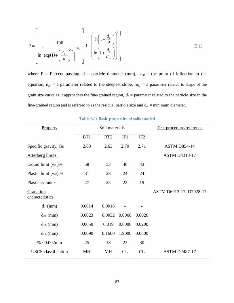
87

7

1ln

1ln

1

1expln

100P

m

r

r

mn

gr

d

d

d

d

d

agr

gr

(3.1)

where P = Percent passing, d = particle diameter (mm), agr = the point of inflection in the

equation, ngr = a parameter related to the steepest slope, mgr = a parameter related to shape of the

grain size curve as it approaches the fine-grained region, dr = parameter related to the particle size in the

fine-grained region and is referred to as the residual particle size and dm = minimum diameter.

Table 3.1: Basic properties of soils studied

Property Soil materials Test procedure/reference

BT1 BT2 JF1 JF2

Specific gravity, Gs 2.63 2.63 2.70 2.71 ASTM D854-14

Atterberg limits: ASTM D4318-17

Liquid limit (wL)% 58 53 46 43

Plastic limit (wP),% 31 28 24 24

Plasticity index 27 25 22 19

Gradation

characteristics:

ASTM D6913-17, D7928-17

d10(mm) 0.0014 0.0016 - -

d30 (mm) 0.0023 0.0032 0.0060 0.0020

d50 (mm) 0.0050 0.019 0.8000 0.0200

d60 (mm) 0.0090 0.1600 1.9000 0.0800

% <0.002mm 25 18 23 30

USCS classification MH MH CL CL ASTM D2487-17

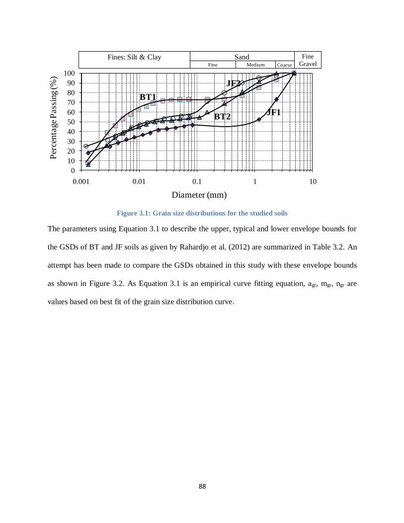
88

Figure 3.1: Grain size distributions for the studied soils

The parameters using Equation 3.1 to describe the upper, typical and lower envelope bounds for

the GSDs of BT and JF soils as given by Rahardjo et al. (2012) are summarized in Table 3.2. An

attempt has been made to compare the GSDs obtained in this study with these envelope bounds

as shown in Figure 3.2. As Equation 3.1 is an empirical curve fitting equation, agr, mgr, ngr are

values based on best fit of the grain size distribution curve.

0

10

20

30

40

50

60

70

80

90

100

0.001 0.01 0.1 1 10

Per

cen

tage

Pass

ing (%

)

Diameter (mm)

Fines: Silt & ClayFine Medium

Sand Fine

GravelCoarse

JF2

BT1

BT2JF1

89

(a)

(b)

Figure 3.2: Grain size distributions: a) BT and b) JF soils in comparison with the upper and lower

bound GSDs and typical GSD.

0

10

20

30

40

50

60

70

80

90

100

0.001 0.01 0.1 1 10

Per

cen

tage

Pass

ing (%

)

Diameter (mm)


Sand Fine

GravelCoarse

BT1

BT2Lower bound

Typical

upper bound

0

10

20

30

40

50

60

70

80

90

100

0.001 0.01 0.1 1 10

Per

cen

tage

Pass

ing (%

)

Diameter (mm)


Sand Fine

GravelCoarse

JF2

JF1

Lower bound

Typical

upper bound

90

Table 3.2: Parameters defining the GSD envelopes for BT and JF formations (from Rahardjo et al.,

2012)

Formation

GSD

bound

envelopes

agr ngr mgr dr (mm) dm(mm)

Lower 1.68 1.66 0.98 20 0.002

BT Typical 2.56 1.94 0.28 20 0.0005

Upper 0.0001 0.58 5.85 9.57 0.0001

Lower 1.25 1.38 0.7 0.010 0.0005

JF Typical 1.23 1.13 0.35 5.00 0.0004

Upper 0.006 1.06 1.13 0.00001 0.001

Figure 3.2 indicates that the GSDs of the soils used in this study are within the upper and lower

GSD bounds suggested by Rahardjo et al. (2012) except for JF1 showing the higher variability of

soils in the Jurong Formation compared to Bukit Timah Granite.

3.3 Compaction behavior and preparation of test specimens

3.3.1 Justification for use of compacted materials

Compaction is a densification process of soils by application of a mechanical energy. According

to Tarantino and De Col (2008), the compaction process may be regarded as a fabrication

process for soils where the soils undergo stress and phase changes. In this study, stress or phase

evolution during compaction was not studied.

The test specimens used in this study were all dynamically compacted residual soils. The reason

for using compacted soils in this study is two-fold. First, they are widely used in many civil

engineering projects including dams, embankments, back fills and pavements. In fact, compacted

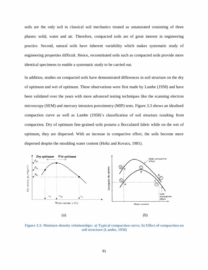
91

soils are the only soil in classical soil mechanics treated as unsaturated consisting of three

phases: solid, water and air. Therefore, compacted soils are of great interest in engineering

practice. Second, natural soils have inherent variability which makes systematic study of

engineering properties difficult. Hence, reconstituted soils such as compacted soils provide more

identical specimens to enable a systematic study to be carried out.

In addition, studies on compacted soils have demonstrated differences in soil structure on the dry

of optimum and wet of optimum. These observations were first made by Lambe (1958) and have

been validated over the years with more advanced testing techniques like the scanning electron

microscopy (SEM) and mercury intrusion porosimetry (MIP) tests. Figure 3.3 shows an idealised

compaction curve as well as Lambe (1958)’s classification of soil structure resulting from

compaction. Dry of optimum fine-grained soils possess a flocculated fabric while on the wet of

optimum, they are dispersed. With an increase in compactive effort, the soils become more

dispersed despite the moulding water content (Holtz and Kovacs, 1981).

(a) (b)

Figure 3.3: Moisture-density relationships: a) Typical compaction curve, b) Effect of compaction on

soil structure (Lambe, 1958)

92

Many studies have observed aggregation of the compacted soil most pronounced on the dry of

optimum side (Delage et al., 1996; Cuisinier and Laloui, 2004; Frydman and Baker, 2009;

Monroy et al., 2009) and that these structures have large influences on mechanical and hydraulic

behaviour of the soils. Furthermore, studies on pore size distributions have concluded that at the

dry of optimum and optimum water contents, soils may possess a dual-porosity or double

structure while soils on the wet of optimum possess a unimodal pore size distribution (Ahmed et

al., 1974; Delage et al., 1996).

Therefore, in addition to studying unsaturated soil behavior, compacted soils make it possible to

study the influences of structure on the mechanical and hydraulic behaviour of soils.

3.3.2 Preparation of test specimens

Prior to compaction, the residual soils were air dried, disaggregated and thoroughly mixed to

form homogenous soil samples. The homogenous soil was then sieved through the ASTM sieve

No. 4 (4.75mm).

In all cases, the soil materials passing sieve No. 4 were thoroughly hand-mixed with distilled

water at targeted water contents. After thorough mixing with distilled water, the soils were sealed

in ziplock plastic bags and stored in a high humidity chamber for at least 120 hours to allow for

moisture equilibration.

The soil materials were then compacted using standard and modified Proctor energies in

accordance to ASTM D698-12 and ASTM D1557-12, respectively, to obtain the moisture-

density relationships for the soil materials at the two energy levels. Figure 3.4 shows the

moisture-density relationships for each of the four soils (BT1, BT2, JF1 and JF2).Table 3.3

summarises the compaction characteristics of the different materials

93

Table 3.3: Compaction properties of soils studied

Property

Soil materials

BT1 BT2 JF1 JF2

Standard Proctor test

Optimum moisture content, % 16 19 18 16

Maximum dry density, Mg/m3 1.69 1.71 1.65 1.76

Modified Proctor test

Optimum moisture content, % 13 13 15 13.5

Maximum dry density, Mg/m3 1.86 1.88 1.83 1.94

Most of the tests done in this study are for cylindrical specimens of about 50mm diameter and

100 mm height. In order to obtain such test specimens, samples compacted in the standard mould

need to be trimmed. Trimming of compacted samples would not only be very cumbersome and

time consuming but more importantly, it would be very difficult to obtain good quality test

specimens especially on the dry side of optimum. Therefore, a two-part split cylindrical plastic

mould (internal diameter = 52mm, height = 102mm) was fabricated so that the test specimens of

the correct diameter are compacted directly. To ensure easy extraction of the compacted

specimen from the split mould, each half of the mould has holes of 1mm diameter drilled in a

grid fashion to allow escape of trapped air during compaction as well as to reduce the side

friction.

94

Figure 3.4: Moisture-density relationships for the soils studied at both standard and modified

Proctor energies

In order to compact the test specimen in the plastic mould, a frame was set up using slotted angle

bars fastened with nuts and bolts as shown in Figure 3.5. The frame was equipped with a pulley

system where a nylon rope was used to lift a drop mass. The drop mass weighed 4.5 kg and has

dimensions of 75mm diameter and 150mm in height. The drop mass has a central hole (diameter

26.5mm that slides along a 26 mm external diameter PVC tube. The PVC tube as shown in

Figure 3.3 is fitted onto a spindle on top of a solid cylindrical steel bar, diameter 51.6mm. The

solid bar rests on top of the soil in the mould and hence transfers the impact energy to the soil.

The PVC tube guide ensures that the drop mass falls centrally on the solid cylindrical steel bar

which then transfers the impact energy to the soil material in the plastic mould.

1.4

1.6

1.8

2

5 10 15 20 25 30

Dry

den

sity

, Mg/m

3

Compaction water content, %

S=60% S=80%

S=100%

S=40%

BT1

1.4

1.6

1.8

2

5 10 15 20 25 30

Dry

den

sity

, Mg/m

3


S=60% S=80%

S=100%

S=40%

BT2

1.4

1.6

1.8

2

5 10 15 20 25 30

Dry

den

sity

, Mg/m

3


S=60% S=80%

S=100%

S=40%

JF1

1.4

1.6

1.8

2

5 10 15 20 25 30

Dry

den

sity

, Mg/m

3


S=60% S=80%

S=100%

S=40%

JF2

95

Using Equation 3.2, the height of drop of the drop mass was calibrated to deliver standard and

modified Proctor energies (ASTM standard and modified Proctor energies are 600 and 2700kN-

m/m3, respectively) to the soil specimen. For the standard Proctor energy, the drop mass was

dropped through a height, h = 200mm and the soil was compacted in three layers while for the

modified Proctor energy, the drop mass was dropped through a height, h = 450mm, and the soil

was compacted in five layers. For both compaction energies, each layer in the plastic mould was

subjected to six blows. Table 3.4 shows a comparison of the ASTM compaction procedures and

those followed in this thesis

Table 3.4 Comparison between the ASTM and thesis procedures of compaction

Item compared

ASTM Procedure Thesis procedure

Standard

Proctor

Modified

Proctor

Standard

Proctor

Modified

Proctor

Mould dimension

(mm)

Ht =116.4

Dia =101.6

Ht = 102

Dia = 52

Rammer weight (kg) 2.5 4.5 4.5 4.5

Rammer drop height

(mm)

305 457.2 200 450

Rammer diameter

(mm)

50.8 50.8 75 75

Compaction layers 3 5 3 5

Blows per layer 25 25 6 6

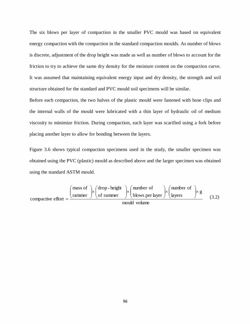
96

The six blows per layer of compaction in the smaller PVC mould was based on equivalent

energy compaction with the compaction in the standard compaction moulds. As number of blows

is discrete, adjustment of the drop height was made as well as number of blows to account for the

friction to try to achieve the same dry density for the moisture content on the compaction curve.

It was assumed that maintaining equivalent energy input and dry density, the strength and soil

structure obtained for the standard and PVC mould soil specimens will be similar.

Before each compaction, the two halves of the plastic mould were fastened with hose clips and

the internal walls of the mould were lubricated with a thin layer of hydraulic oil of medium

viscosity to minimize friction. During compaction, each layer was scarified using a fork before

placing another layer to allow for bonding between the layers.

Figure 3.6 shows typical compaction specimens used in the study, the smaller specimen was

obtained using the PVC (plastic) mould as described above and the larger specimen was obtained

using the standard ASTM mould.

volumemould

glayers

ofnumber

layerper blows

ofnumber

rammer of

height -drop

rammer

of mass

effort compactive

(3.2)

97

(a) Photo

(c) Schematic drawing

(b) Compaction accessories

Figure 3.5: Compaction set-up to prepare soil specimens in the PVC mould

The energy input per unit volume of soil is the same for both the standard ASTM procedure and

the PVC mould procedure adopted in this thesis. In the standard procedures, the 25 blows of

compaction hammer is not directed at only one spot on the top of the sample as it is in the case of

the compaction in the smaller PVC mould. However, the soil sample in the PVC mould

experiences more side friction compared to the soil sample in the standard mould. This made it

difficult to match the dry density on the compaction curve. It is expected that there will be some

difference in the soil structure but the general characteristics of the compacted samples in the

Nylon rope

Drop mass

Pulley

system

PVC guide

Anvil

Soil

Split PVC

2-part

mold

Holder

Slotted angle

bar frame

98

PVC mould and standard mould will be largely the same. When referring to dry of optimum,

optimum and wet of optimum, the optimum moisture content as obtained from the standard

mould is used in this thesis.

Figure 3.6: Typical compaction specimens, left specimen obtained using the PVC mould and the

right specimen using the ASTM standard compaction mould

3.3.3 Nomenclature of the test specimens

As mentioned previously, four soils (two each from BT and JF) were studied. Specimens were

prepared using two different compaction moulds, the standard ASTM mould and the PVC plastic

mould. Additionally, test specimens were compacted at two energy levels, standard and modified

Proctor, and various moulding water contents.

Given these variables, it was important to develop a nomenclature for the test specimens for ease

of reference. The nomenclature adopted is in the form AAx-BBB-CCyy where AA refers to the

formation from which the soil was obtained (BT or JF), x refers to soil 1 or soil 2 from each

formation, BBB refers to compaction energy (STD for standard or MDF for modified), CC refers

to the compaction mold used (ASTM mold or PL plastic mold) and yy refers to the compaction

water content in % go the nearest whole number.

99

For example:

A soil 1 (x = 1) from Bukit Timah (AA = BT) compacted at standard Proctor energy (BBB =

STD) using the standard ASTM mould (CC = ASTM) at a water content of 10% (y = 10) is

designated as : BT1-STD-ASTM10 and if it was compacted at modified energy it is: BT1-MDF-

ASTM10. If the mould was PVC plastic mold, the designation would be BT1-STD-PL10 and

BT1-MDF-PL10.

Table 3.5 further illustrates the nomenclature adopted for the test samples (in the as-compacted

state) for this study.

Table 3.5: A guide to the nomenclature adopted for the different test specimens

Geological

Formation

Compaction effort Compaction mould Compaction water

content, %

BT1, BT2,

JF1 or JF2

STD= Standard Proctor

MDF= Modified Proctor

ASTM = Standard

compaction mould

recommended by

ASTM

PL= plastic PVC mould

fabricated in this study

e.g 10, 14 et.c

The subsections that follow present the different tests done on in this study. Detailed procedures

are presented for the experiments including the rationale where applicable.

100

3.4 Suction measurements

Two major techniques of suction measurement were employed in the study, filter paper

technique and chilled mirror dew-point technique. The adopted procedures are described below.

3.4.1 Filter paper technique

The filter papers used in this study were Whatman No. 42, ashless type, diameter 42.5mm.

Whatman filter papers were preferred to other brands of ashless filter papers because they are

thicker, have smaller pore sizes (Chandler and Gutierrez, 1986) and can measure suction over a

wide range (Sibley and Williams, 1990).In this study, both contact and non-contact filter paper

methods were used to measure the matric and total suctions, respectively. Both initially dry and

initially wet Whatman No.42 filter papers of 42.5mm diameter were used.

In this thesis, the following notations have been adopted to identify the filter paper condition:

ID-C-FP for initially dry contact filter paper, ID-NC-FP for initially dry non-contact filter paper,

IW-C-FP for initially wet contact filter paper, and IW-NCFP for initially wet non-contact filter

paper.

3.4.1.1 Initially dry filter papers

Initially dry filter papers were used as obtained directly from their boxes without any pre-

treatment. The average initial water content of Whatman No. 42 filter papers was found by oven

drying 48 pieces of the filter paper and found to be 6.6% with a standard deviation of 0.8%.

Marinho and Oliveira (2006) reported an average initial water content of about 6% for Whatman

No. 42 filter paper.

101

3.4.1.2 Initially wet filter papers

Most of the literature reported the use of initially dry filter paper to measure soil suction. The

procedures suggested in ASTM D5298-16 are for an initially dry filter paper, in fact ASTM

D5298-16 suggests oven-drying the filter paper prior to its use. A few researchers (e.g Muñoz-

Castelblanco et al., 2010; Acikel et al., 2015; Leong et al., 2016) have examined the use of an

initially wet filter paper to examine its possible advantages over initially dry filter paper. These

studies indicate good potential for the use of initially wet filter paper for suction measurement.

The inclusion of the initially wet filter paper in the test programme of this study followed the

hypothesis that an initially wet filter paper reduces the equilibrium time, hence would reach

equilibrium faster than an initially dry filter paper. Therefore, this thesis presents the test results

of suction measurements using both initially dry and initially wet Whatman No. 42 filter papers.

More than 1700 pieces of filter papers were used. The performances of initially dry and initially

wet filter papers are assessed and are compared for the measurement of both matric and total

suctions. In addition, equilibrium time, hysteresis and other factors influencing the measurement

are evaluated.

Two methods were adopted in the preparation of the initially wet filter papers. In Method 1, the

filter papers were initially soaked in distilled water for about 45 minutes and then left to dry over

a saturated sodium chloride (NaCl) solution in an airtight desiccator for two hours. The room

temperature varied between 24 and 26oC, hence the relative humidity in the desiccators was

expected to be about 76% (Young, 1967).

In Method 2, the filter papers were initially soaked in distilled water for about 45 minutes and

then left to dry to water contents of between 40 and 70%over saturated NaCl solution in an

airtight desiccator. This range of water content covers the region between the total suction and

matric suction calibration curves of the Whatman No. 42filter paper.

102

For both Methods 1 and 2, the suction measured by the initially wet filter paper was compared to

the suction measured by an initially dry filter paper. In Method 1, only specimens compacted in

the standard mould were used as suction sources for the filter paper while in Method 2,

specimens compacted in the plastic mould were used.

Filter paper handling and soil specimen preparation

In all cases, the filter papers, were handled using a clean pair of tweezers with gloved hands to

ensure no contamination of the filter papers (Bulut et al., 2001). Airtight containers, internal

diameter of 85 mm and height of 70 mm, were used to contain the soil specimen for equilibration

with the filter paper. Regardless of the type of mould used, soil specimens were carefully

trimmed from the compacted samples such that they occupied at least 75% of the volume of the

airtight containers. Trimming the plastic mould compacted samples was easier than trimming the

standard mold compacted samples. The cylindrical specimens were sliced at mid-height and a

contact filter paper was sandwiched between the two halved specimens (Figure 3.7a). The soil

specimen was then wrapped in three layers of cling film leaving only the top surface exposed

when placed into the airtight container (Figure 3.7b). A PVC ring (diameter 40 mm and

thickness 5 mm) was placed on top of the soil specimen onto which a piece of non-contact filter

paper was placed (Figure 3.7b). The airtight container was then sealed and kept in a Styrofoam

box (Figure 3.7c) where the filter paper was left to equilibrate with the soil specimen for

different durations ranging from 7 to 60 days.

Determination of soil suction from the filter paper water content

At the end of each duration, the contact and non-contact filter papers were retrieved and their

water contents were determined (Bulut et al., 2001).Prior to removing a filter paper, the mass of

103

a clean ziplock plastic bag was determined on a sensitive electronic balance (of accuracy

0.00001g) as shown in Figure 3.8 (a) and was recorded as M1.The ziplock bag was cleared of any

trapped air on a clean flat surface. With the mass of the ziplock bag known, the filter paper was

transferred as fast as possible (less than 5 second) into the ziplock bag. The weight of the ziplock

bag and filter paper together was determined as shown in Figure 3.8 (c) and recorded as M2. In

all cases the filter paper was handled using a clean pair of tweezers. The ziplock bags were

handled using gloved hands to ensure no sweat or dirt was added to the ziplock bag. For the case

of the contact filter paper (sandwiched), the filter paper was quickly removed, cleared of any

loose soil particles using a clear soft brush as shown in Figure 3.8 (b) and then transferred into

the ziplock bag for weighing.

104

( a) (b)

(c)

Figure 3.7: Preparation of soil specimen for suction measurement using filter paper technique

The weighed filter paper was then transferred to a crucible (Figure 3.8d) and placed in the oven

to dry (Figure 3.8e). In all cases, the label of the porcelain bowl was recorded against the soil

specimen identity as well as the type of suction being tested (contact filter paper for matric and

non-contact for total suction).In all cases, the crucibles were left half open while in the oven to

allow the filter paper to dry.

105

(a) (b) (c)

(d) (e)

Figure 3.8: Filter paper handling post equilibration.

At the end of the drying, the cover of the crucible was then fully replaced and allowed to stay in

the oven for about three minutes to allow for thermal equilibrium. The crucible containing the

filter paper was then removed from the oven and placed in a desiccator to cool.

The filter paper was re-weighed. As before, the weight of the ziplock bag was determined on an

electronic balance and recorded as M3. The oven-dried filter paper was then transferred to the

pre-weighed ziplock bag using tweezers and gloved hands and the weight of both the ziplock bag

and filter paper was determined and recorded as M4. In cases where ziplock bags were re-used,

they were always re-weighed to re-establish their weights. Ziplock bags were never re-used if

their weights between consecutive measurements differed by more than 0.00005g. For non-

106

contact filter papers, this was usually after three times of use while for contact filter papers, it

was once or maximum twice, largely dependent on the level of contamination.

The filter paper water, fw , content in all cases was computed as using Equation 3.3.

%100

MM

MMMMw

34

3412

f

(3.3)

With the filter paper water content obtained, soil suction was obtained using Whatman No.42

filter paper calibration equations by Leong et al. (2002b)given in Equations 3.4 and 3.5.

Matric suction 47 w, 0.0673w-4.945logψ

47 w, 0.0229w-2.909logψ

f f

ff

(3.4)

Total suction 26 w, 0.0879w-5.31logψ

26 w, 0.222w-8.778logψ

f f

ff

(3.5)

In addition the moisture content of the soil sample was also determined according to ASTM

D2216-10 and hence the computed suction is matched with the soil moisture content.

3.4.2 Chilled mirror dew-point technique

In addition to using the filter papers, independent suction measurements were done on selected

soil specimens using the chilled mirror dew-point (CMDP) technique following procedures

suggested by Leong et al. (2003). Agus and Schanz (2005) evaluated four methods commonly

used in the measurement of total suction and found the CMDP technique is the most reliable if

used under a strict protocol. They suggest CMDP as a benchmark for assessing other techniques.

The WP4C dew-point hygrometer from Decagon Devices set in precision mode was used. The

device was switched on for at least 30 minutes prior to use to allow it to warm up and the sample

cups were always ensured to be cleaned. Test specimens were trimmed from the larger

compacted samples and placed in the sample cups. It was ensured that the quantity of the test

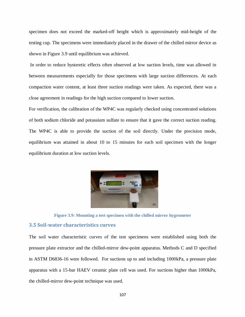
107

specimen does not exceed the marked-off height which is approximately mid-height of the

testing cup. The specimens were immediately placed in the drawer of the chilled mirror device as

shown in Figure 3.9 until equilibrium was achieved.

In order to reduce hysteretic effects often observed at low suction levels, time was allowed in

between measurements especially for those specimens with large suction differences. At each

compaction water content, at least three suction readings were taken. As expected, there was a

close agreement in readings for the high suction compared to lower suction.

For verification, the calibration of the WP4C was regularly checked using concentrated solutions

of both sodium chloride and potassium sulfate to ensure that it gave the correct suction reading.

The WP4C is able to provide the suction of the soil directly. Under the precision mode,

equilibrium was attained in about 10 to 15 minutes for each soil specimen with the longer

equilibrium duration at low suction levels.

Figure 3.9: Mounting a test specimen with the chilled mirror hygrometer

3.5 Soil-water characteristics curves

The soil water characteristic curves of the test specimens were established using both the

pressure plate extractor and the chilled-mirror dew-point apparatus. Methods C and D specified

in ASTM D6836-16 were followed. For suctions up to and including 1000kPa, a pressure plate

apparatus with a 15-bar HAEV ceramic plate cell was used. For suctions higher than 1000kPa,

the chilled-mirror dew-point technique was used.

(a)

(b)

(c)

108

3.5.1 Pressure plate tests

The pressure plate system consists of a pressure chamber which contains a saturated HAEV

ceramic disk. Beneath the ceramic disk is attached a neoprene rubber sheet which provides a

hydraulic continuity between the saturated ceramic disk and a water burette outside the air-

pressure chamber (Leong and Rahardjo, 2002) as shown in Figure 3.10.

The test specimens for the SWCC test using pressure plate were pre-saturated. The specimens

compacted in the plastic mould were saturated following the procedure suggested by Samingan

(2001). In this procedure, the compacted specimens were allowed to absorb water freely with

close monitoring of their masses to ensure saturation. In order to limit lateral swell the samples

were wrapped in four layers of plastic film. Whatman No. 54 filter papers were placed on both

the top and bottom of the specimens to protect the specimens from erosion by the water. The

specimens were then placed on wetted cotton wool in a plastic box. The specimens absorbed

water from the wetted cotton wool. At the end of the saturation, the saturated samples were

trimmed to obtain the test specimens. For the pressure plate test, cylindrical specimens of 50 mm

diameter and 30 mm height were used.

(a) Schematic b) Picture

Figure 3.10: Pressure plate system

Air Chamber

Burette

Stand

Soil Specimens

Pressure plate cell

109

For the specimens compacted in the standard mould, the specimens for SWCC test were those

obtained from the flexible wall permeameter test as will be discussed later.

The dimensions and weight of saturated soil specimens were determined and then placed onto

the saturated ceramic disk. The test suction levels in the pressure plate were increased

incrementally from 10 to 1000kPa in pressure steps as recommended in ASTM D6836-16. The

weights of the soil specimens were monitored daily. Equilibrium at a given suction level was

attained when there was negligible change in the weight of the specimen. At equilibrium, the

dimensions of the specimen were noted as well. Suction level was then increased to the next

suction by adjustment of the air pressure. Finally, the water content of the soil specimen at

equilibrium with each matric suction level was established in order to construct its SWCC.

3.5.2 Chilled mirror dew-point test

For suctions higher than 1000kPa, the chilled-mirror dew-point technique following Leong et al.

(2003) was used. For this test, a cylindrical disk specimen of diameter 35mm and thickness 5mm

was cookie-cut from the sample at the end of the saturation process using a PVC ring with a

sharpened edge and placed in sample cups used for the chilled-mirror dew-point test.

These samples were dried in air-tight desiccators with saturated sodium chloride solution at the

base of the desiccators. The room temperature varied between 24 and 26oC, hence the relative

humidity generated in the air-tight desiccators was expected to be approximately 76% (Young,

1967). The weights of the sample cups with the soil were monitored periodically as the soil dries.

At the same time, the soil’s suction was measured using the WP4C dewpoint hygrometer set in

the precision mode. The drying continued until no further change in weight could be observed

meaning the soil had reached equilibrium with the saturated salt solution. The sample cups with

110

the soil were then transferred to the open environment of the laboratory to allow for further

drying until no further weight change could be recorded, each time measuring the suction of the

test specimen using the WP4C.

As mentioned earlier, the WP4C measures the suction directly the Kelvin equation re-stated as

Equation 3.6.

)(Rlnωv

RTψ h

vw0

(3.6)

where = total suction (kPa), R = universal gas constant (8.314232 J/mol K), T = absolute

temperature (K), vw0 = specific volume of water, v = molecular mass of water vapour (18.016

kg/kmol) and hR = relative humidity.

Similar to the pressure plate test, the specimen’s water contents at equilibrium with the measured

suctions were established and combined with those from the pressure plate test to obtain a

complete SWCC for each soil specimen.

3.6 Hydraulic properties of compacted soils

Two sets of experiments were performed in order to study the hydraulic properties of compacted

soils, infiltration test using a mini-disk infiltrometer and measurement of saturated permeability

using the flexible wall permeameter (FWP).

3.6.1 Infiltration test using a mini-disk infiltrometer

The mini-disk infiltrometer used in this study (Decagon Devices, 2014) can be adjusted from -

0.5 to -7cm of pressure head. In this study, the infiltration tests were done on compacted soils in

the laboratory by placing the infiltrometer on top of the compacted soil as extruded from the

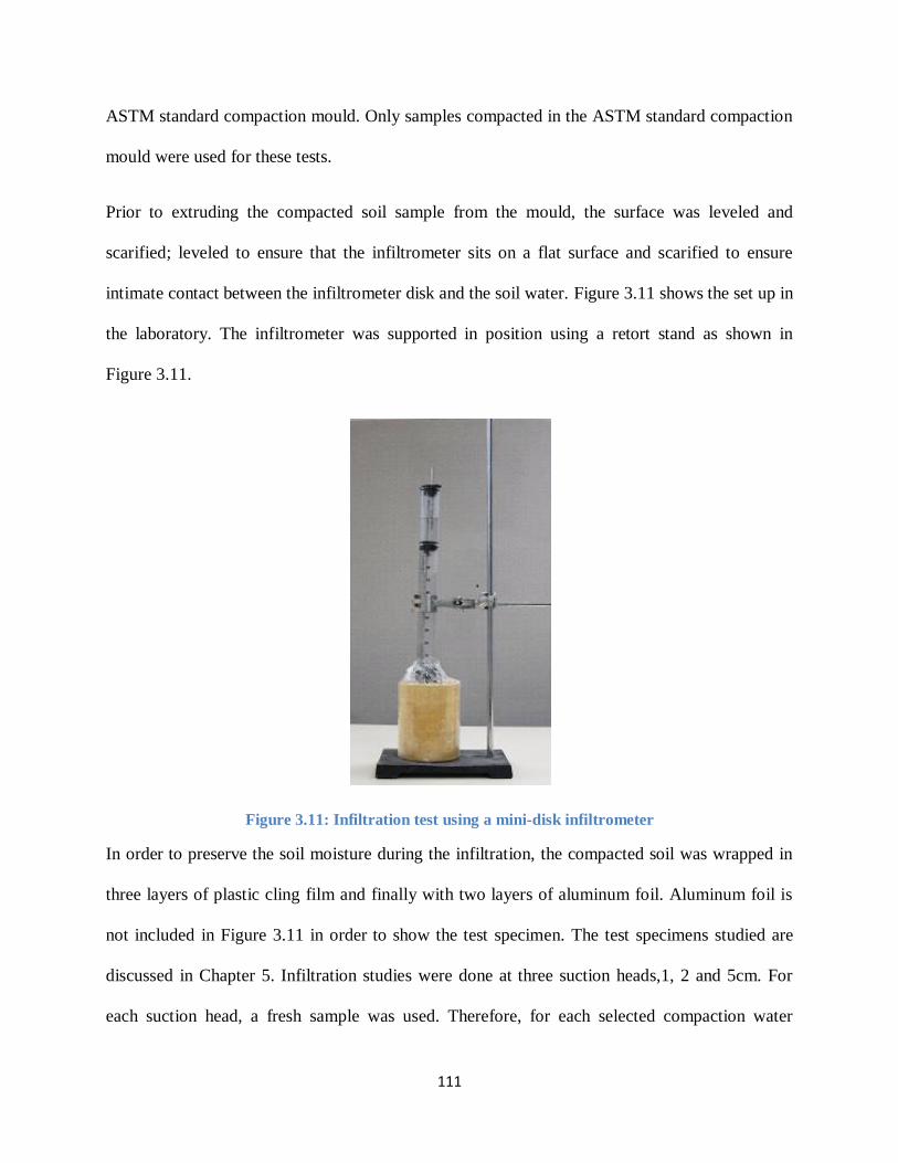
111

ASTM standard compaction mould. Only samples compacted in the ASTM standard compaction

mould were used for these tests.

Prior to extruding the compacted soil sample from the mould, the surface was leveled and

scarified; leveled to ensure that the infiltrometer sits on a flat surface and scarified to ensure

intimate contact between the infiltrometer disk and the soil water. Figure 3.11 shows the set up in

the laboratory. The infiltrometer was supported in position using a retort stand as shown in

Figure 3.11.

Figure 3.11: Infiltration test using a mini-disk infiltrometer

In order to preserve the soil moisture during the infiltration, the compacted soil was wrapped in

three layers of plastic cling film and finally with two layers of aluminum foil. Aluminum foil is

not included in Figure 3.11 in order to show the test specimen. The test specimens studied are

discussed in Chapter 5. Infiltration studies were done at three suction heads,1, 2 and 5cm. For

each suction head, a fresh sample was used. Therefore, for each selected compaction water

112

content, three specimens were compacted ensuring that they are identical in terms of water

content and dry density. The water content variation was controlled to be within ±0.2%. Only

specimens meeting these criteria were used for the tests.

3.6.2 Falling head flexible-wall permeameter

At the end of the infiltration test, one of the three specimens for each compaction water content

was trimmed to obtain a specimen of diameter 50mm and height 40 mm. The soil specimen was

then transferred into a flexible-wall permeameter and a falling-head test was conducted with

water flow upwards from the base of the soil specimen. This ensured that the air in the soil voids

was flushed out by upward displacement since air is less dense than water. Figure 3.12 shows the

experimental set up.

Schematic (after Samingan, 2001)

Figure 3.12: Flexible wall permeameter set up

113

In the permeameter, a de-aired porous stone was placed on the base pedestal, on top of which a

filter paper (Whatman No.54) dipped in water (the permeant liquid) was placed. The soil

specimen was placed on the filter paper. Similarly, another filter paper was placed on top of the

soil specimen followed by another de-aired porous stone. A top cap (with drainage lines initially

disconnected) was placed on to the top porous stone.

After placement of the top cap, a latex membrane was placed on to the soil specimen using a

membrane stretcher. During placement of the membrane, it was ensured that the membrane

extended from the bottom of the base pedestal to the top cap. The membrane was held in place

by two O-rings; one placed on the base pedestal and the other on to the top cap. It was important

that the membrane was firmly stretched so that no water flow occurs between the sides of the

specimen and the membrane which would lead to an over estimation of the permeability. Any

length of the membrane that extends above the top cap was rolled off and drainage lines

connected to the top cap.

The cell wall was then replaced and the cell was filled with water. A nominal confining pressure

of 10kPa was applied to support the specimen. Finally, the base of the specimen was connected

to water line supplied from a burette as shown in Figure 3.12.

The water levels on the graduated burette were monitored at regular time intervals. For each

specimen, several runs of the test were done. For each run, the burette was re-filled and hydraulic

head drops, h, was monitored with time. This continued until a steady state was attained. Steady

state was evaluated using Equation 3.7.

2.303aL

Aktloghlogh 0 (3.7)

114

where h is the hydraulic head at time t while h0 is the original hydraulic head (t=0). All hydraulic

heads were referred to the tail water set at the base of the specimen.

Equation 3.7 is linear with a negative slope =2.303aL

Ak. With several runs done, a constant ks was

assumed to have been attained as the slopes of Equation 3.7 for the consecutive runs became

very close or a constant value.

The saturated permeability, ks, was obtained from the steady state slope, mst as shown in

Equation 3.8

A

m*2.303aLk st

s (3.8)

For all the tests, the filter papers were cut to a diameter of 50mm which was equal to the

diameter of the test specimen. The use of the filter papers was to ensure that the porous stones

were not clogged by soil particles during the test. Prior to the test, the porous stones were soaked

in water and placed in a vacuum desiccator for 24 hours to ensure they were de-aired. De-airing

the porous stones ensured the stones were fully saturated.

3.7 Strength tests

Four strength tests were done on the compacted soils. Three were done on the as-compacted soil

specimens and one test was done on the saturated test specimens in order to obtain the saturated

shear strength parameters, the friction angle and the cohesion. Only specimens compacted in the

plastic mould were tested for strength. The strength tests used in this study are described below.

115

3.7.1 Unconfined compression test

Given that the unsaturated soils often occur at shallow depths from the surface with very small

confinement, unconfined compressive (UC) strength is useful in studying shear strength behavior

of soils. Two series of experiments were conducted for the UC test. The first series involved the

as-compacted soils at various water contents on both the standard and modified Proctor curves.

The water contents selected for each soil are detailed in Chapter 6. In the first test series, the

compacted soils were sheared immediately after compaction to obtain the as-compacted

unconfined compressive strength.

The second test series was done on BT1, BT2 and JF2 as described in Chapter 6. This series of

experiments involved soils compacted at wet of optimum on both the standard and modified

Proctor curves. The test specimens were then dried in desiccators with saturated sodium chloride

(NaCl) solution at the base of the desiccators. The saturated NaCl solution provides a constant

relative humidity of about 76% (Young, 1967) to dry the test specimens. The test specimens

were laid lengthwise over the saturated NaCl solution to minimize moisture gradients that may

develop if placed upright and hence ensure more uniform drying of the test specimens. The

weights of the specimens were monitored regularly. Specimens that attained the targeted weight

(and hence moisture content) were wrapped in cling film and thereafter kept in a temperature-

controlled humidity chamber to allow for moisture equalization in the test sample for about 10

days as recommended by Mendes (2011). The specimens were then sheared according to ASTM

D2166-16 to obtain the unconfined compressive strength qu. Prior to shearing, the dimensions of

the specimens were measured for density, shear strength and volumetric shrinkage computations.

After shearing, the moisture content of the test specimen were determined. It should be noted

that all the UC tests were performed at atmospheric pressure i.e. ua=0

116

Assuming 0 zx , the unconfined compressive strength, y was computed using Equation

3.9

A

Py

(3.9)

where P = peak load, and A= cross sectional area of the specimen.

3.7.2 Brazilian tensile strength test

Similar to the UCS test, the Brazilian tensile strength (BTS) test was also done in two test series.

Similar moisture contents and densities as used for the UCS tests were used. To obtain BTS test

specimens, samples compacted in the plastic mold were sawn using BuehlerIsoMet™ 4000

precision saw into cylindrical disk specimens of 30mm thick and 52mm diameter. Although the

precision saw can minimize sample deformation and have low kerf loss, the compacted samples

were wrapped in two layers of cling film followed by a single layer of masking tape along the

sample height to prevent moisture loss and to limit surface cracking during sawing. Figure 3.13

shows a sample prepared for sawing. Three specimens were obtained from each compacted

sample. The ASTM D3967-16 which is for rock core specimens was used as a guide for the BTS

test. The thickness to diameter (t/d) ratio of the test specimens was maintained as close to 0.6as

possible, within the recommended range of 0.2 to 0.75 in ASTM D3967-16.The test specimens

for the BTS were loaded using two specially fabricated curved bearing blocks as recommended

in ASTM D3967-16 to reduce contact stresses on the specimens during the test. The radii of

contact arc with the test specimen was 10o while the width of contact with the specimen was

30mm. During testing, the bearing blocks were attached to the loading platens of the UCS testing

machines using magnets embedded into the base of the bearing block as shown in Figure 3.14.

117

Figure 3.13: Compacted sample prepared for sawing to obtain BTS test specimens

a) Test set up b) Loading on soil disk

c) Curved bearing block

Figure 3.14: Test set-up and curved block for Brazilian tensile test

yσ

xσ

x

P

y

Z

10°

50 mm

10 mm

20 mm20 mm

10 mm

20 mm

Magnet

118

The BTS test was conducted at a loading rate of 0.5mm/min as recommended by Akin and Likos

(2017) and all test specimens failed within 1 to 10 minutes (ASTM D3967-16).Assuming plane

stress state at the centre of the BTS specimen, a closed-form elastic solution for the stress state in

a BTS specimen at failure (Frydman, 1964, Akin and Likos, 2017) is given by Equations (3.10)

πtd

2P tx

(3.10a)

πtd

6.2P1.3σ y x

(3.10b)

0z (3.10c)

where P= peak compressive load at failure, d = average diameter of the soil specimen, t =

average thickness of the specimen, x = the tensile strength of the specimen, and y , z are

normal stresses in the y and z directions, respectively.

3.7.3 Unconsolidated undrained test

The Unconsolidated undrained (UU) test was performed only on the as –compacted soil samples

(test series 1). The test was done in accordance to ASTM D2850-15. Unlike the unconfined

compression test described above, in this test soil specimens were subjected to a confining

pressure. Three confining pressures were used 70kPa, 150kPa, 300, and 600kPa, elected with an

aim to cover a wide range of confinement and hence investigate the soil response over the range.

The UU test was conducted with air phase drained at atmospheric pressure and water phase

undrained hence the test was a constant water (CW) test. Allowing for air drainage but not water

drainage means the sample volume changes which simulates typical construction practices in

which compacted layers are usually loaded fast enough not allowing water drainage however air

will drain. The shearing was done at a rate of 1.57mm/min. The test was stopped when either a

distinct shear plane was observable or substantial vertical deformation had been observed for wet

119

samples or at high confinement pressures. The extent of deformation allowed was also governed

by the load ring capacity.

At the end of the test, the soil specimen was removed from the chamber and its moisture content

determined in accordance with ASTM D2216-10.Data processing followed ASTM D2850-15

with membrane corrections performed as well as the area corrections.

3.7.4 Consolidated undrained test for saturated soils

In order to obtain the effective strength parameters i.e. ϕ’ and c’, consolidated undrained (CU)

tests with pore-water pressure measurements were performed on the as-compacted soil

specimens. The CU tests were performed in accordance to ASTM D4767-11. Because of the

time duration required for saturation and also due to the high variability of dynamically

compacted soils, the CU test was performed using the multistage technique closely following

recommendations of Head (1998). According to Head (1998), the multistage testing is suitable

for soils with low sensitivity, stable structure and those that fail at low strain levels all of which

are largely satisfied by the soil specimens in this study.

Saturation of the soil specimens was done by applying back pressure and cell pressure while

measuring the pore-water pressures developing in the samples in order to calculate Skempton B-

parameter. In order to hasten the saturation, the samples were pre-saturated in a desiccator with

application of a very small vacuum to ensure as much air as possible is displaced from the soil

sample before being set up in the triaxial system. In addition, the porous stones were de-aired in

a vacuum desiccator to ensure they were saturated. Drainage lines of the triaxial system were

flushed by applying a water pressure of about 50kPa to eliminate all the entrapped air.

120

The samples were again saturated in the triaxial cell and considered to be saturated when the B-

parameter was at least 0.96 (Head 1998). Multistage testing was done in three stages at effective

confining pressures: 80, 150 and 300kPa, respectively. At each stage, the specimens were

consolidated at the effective confining pressure before shearing. Volume of water expelled from

the specimens during consolidation was noted using a burette and used in volume, area and

length corrections at each stage. ASTM D4767-11 suggests a procedure for computing a shearing

rate using consolidation data of the specimen. After doing some trials on a couple of test

specimens, a shearing rate of 0.01mm/min was adopted. The same shearing rate was used for all

the stages of the multistage technique. For the first and second stages, it was ensured that the

axial strain never exceeded 6 and 2%, respectively, after which the sample was unloaded very

fast. In the third stage, the specimen was sheared to failure. Failure was considered to have

occurred when deviator stress began dropping. For samples that had no definite failure, deviator

stress at 20% was considered as failure load.

The data processing followed ASTM D4767-11 as well as Head (1998). All appropriate area and

membrane corrections were done.

121

Chapter 4. Soil Suction measurements and Soil-Water Characteristic

Curves

4.1 Introduction

Suction measurement is important in evaluating and understanding the engineering behavior of

unsaturated soils. This chapter presents and discusses experimental results from suction

measurements made on the as-compacted soils as well SWCCs of the compacted soils. The main

technique for suction measurement is the filter paper (FP) technique. More suction

measurements were made using the chilled mirror dew-point (CMDP) technique for the purpose

of comparison as recommended by Agus and Schanz (2005).The soil-water characteristic curve

(SWCC) as discussed in Chapter 2 is key to the implementation of unsaturated soil mechanics.

The SWCC shows the variation of soil water content with suction for a given soil. Because

different compaction water contents result in different soil structures and hence different soils,

influences of compaction on SWCCs are studied. Finally, a comparison between suction

measurements derived from the SWCC and those obtained from suction measurements with the

FP is made.

4.2 Suction measurements using the filter paper method

Suction measurement methods still face several challenges such as cost, measurement range,

equilibrium time and reliability. Among the indirect suction measurement methods, the filter

paper method offers many advantages as discussed in Chapter 2. However, despite its

advantages, the filter paper technique has several shortcomings such as inherent variability, low

sensitivity at low suctions, long equilibrium time, and reliability of results.

In this thesis, an attempt is made to study the following aspects:

122

1. Equilibration time of the filter paper

2. Influence of initial moisture state of the filter paper on the suction measurement

3. Hysteresis of the filter paper

4. Suction measurements- matric and total suction

5. Inherent variability of the filter paper.

As already emphasized earlier, the suction measurements were done on the as-compacted soils.

Specimens compacted using the standard ASTM mould and the plastic mould were used for

suction measurement. Figure 4.1 shows the moisture-density relationships for the soils.

It should be noted from Figure 4.1 that only BT1, BT2 and JF2 soils were largely used in the

study of suction measurements. Only few measurements were made on JF1 soil whose results

will be used in Chapter 7. Also notable in Figure 4.1 is the comparison between specimens

compacted in the standard ASTM mould and those compacted in the plastic mould. The dry

densities attained using the plastic mould for BT2 and JF2 soils and some points for BT1soil are

lower than those attained using the standard mold. This was largely due to greater side-wall

friction in the plastic mould.

4.2.1 Equilibration time for filter papers

The effect of equilibration time on filter paper water content was done for both the initially dry

and initially wet filter papers in contact and non-contact with BT1 and JF2 soil specimens

compacted using the standard and modified Proctor efforts. Figures 4.2 and 4.3 show the

comparison for BT1 soil specimens while Figures 4.4 and 4.5 show the equivalent plots for JF2

soil specimens.

123

(a) BT1 (b) BT2

(c) JF2

Figure 4.1: Moisture-density relationships for the study materials used in suction measurements

In Figures 4.2 to 4.5, the equilibration time was from 7 to 28 days and the initially wet filter

papers were prepared using Method 1 as described in Chapter 3. Figures 4.2 to 4.5 show that the

equilibrium water content of the filter papers increases as the water content of the compacted

soils increases from dry of optimum to wet of optimum. Figures 4.2 to 4.5 generally show that

1.4

1.6

1.8

2

5 10 15 20 25 30

Dry

den

sity

, Mg/m

3


Standard Mold - Standard Proctor

Standard Mold - Modified Proctor

Plastic Mold - Standard Proctor

Plastic Mold - Modified Proctor

60%80%

S=100%

40%

BT1-soil set

1.4

1.6

1.8

2

5 10 15 20 25 30

Dry

den

sity

, Mg/m

3


Standard Mold-Standard Proctor

Standard Mold-Modified Proctor



60%

80%

S=100%

40%

BT2-soil set

1.4

1.6

1.8

2

5 10 15 20 25 30

Dry

den

sity

, Mg/m

3






60%

80%

S=100%

40%

JF2-soil set

124

the initially dry filter papers exhibit less scatter than the initially wet filter papers for both the

contact and non-contact methods. For soil samples compacted at optimum and dry of optimum

water contents, an equilibration time of 7days seems adequate for initially dry filter papers

regardless of contact condition. This suggests that it is easier for an initially dry filter paper to

wet rather than for an initially wet filter paper to dry. In addition, the higher the suction, the

lower the equilibration time required by the filter paper, confirming the observation of Marinho

and Oliveira (2006).

For soil specimens compacted on the wet side of optimum, the scatter in the filter paper water

contents for both the initially dry and initially wet filter papers increase with increasing

compaction water content. The non-contact filter papers sometimes failed to show equilibrium

indicating that the filter paper failed to give any reliable suction measurements at such water

contents. The initially wet filter paper shows less scatter when used in contact mode compared to

when used in non-contact mode.

The results of the second series of compacted soil specimens (compacted in plastic mould) are

shown in Appendix A1. The equilibration time used in the second series of compacted soil

specimens ranges from 7 to 60 days and the initially wet filter papers were prepared using

Method 2 as described in Chapter 3. Less scatter was observed for the initially wet filter paper

indicating that the fluctuations are due to the preparation of the initially wet filter paper using

Method 1. As a further check, 12 filter papers randomly picked from the same box of Whatman

No. 42 filter papers were soaked in distilled water for 1 hour and thereafter allowed to dry in an

airtight desiccator over a saturated NaCl solution. Their weights were taken at 4, 8 and 24 hours,

after which the water content of the filter papers were determined. Figure 4.6 shows the drying

pattern of the filter papers. Although the water contents of the filter papers seem to converge at

125

24 hours, the scatter in the water contents between 0 and 8 hours reveals wide differences in

drying behavior. These differences in drying of the individual filter papers may partly explain the

scatter observed with the initially wet filter paper prepared using Method 1 especially when used

in the non-contact mode. Generally, the initially wet filter paper requires stricter control of its

initial moisture content and selection of equilibration time especially when used in non-contact

mode to measure total suction.

Leong et al. (2002b) note that equilibration for the non-contact filter paper method is a two-stage

process; first, equilibration between the soil and the environment (air-space), and second, the

equilibration between the environment and the filter paper. Therefore, the initially wet filter

paper is expected to undergo either wetting or drying depending on the suction it is measuring. In

addition, it is expected that initially wet filter paper having water content corresponding to the

suction of the soil would equilibrate faster. Hence, the initially wet filter paper when measuring

the low suction of soils compacted wet of optimum is expected to achieve equilibrium much

quicker especially for total suction compared to initially dry filter paper. However, the

experimental results do not show this benefit.

The performance of the initially wet filter paper seems to be affected by factors not observed in

initially dry filter papers. When the size of the air space above the soil in the container is large, it

may expectedly lead to longer equilibration time and when it is too small, the initially wet filter

paper may fail to achieve equilibrium moisture with the air space. Another possible factor

affecting the initially wet filter paper is the possible modification of the filter paper structure

when wetted thus altering its surface adsorption properties and introducing more variability in

the filter paper.

126

4.2.2 Initial moisture condition of filter paper

As stated in Chapter 3, the most commonly used filter paper method is to use initially dry filter

paper directly from its box. ASTM D5298-16 recommends oven drying the filter papers before

use to ensure zero initial moisture content. Although this may eliminate variability in the initial

water content, it may alter the filter paper characteristics and hence affect its other properties

such as absorption as noted by Marinho and Oliveira (2006). To avoid contamination and

possible attack by microorganisms, ASTM D5298-16 further recommends the filter paper to be

sandwiched between two other filter papers to measure the matric suction of the soil and to use

two filter papers for the total suction. However, using more than one piece of filter paper may

require longer equilibrium time and may result in measuring higher suction especially when used

to measure suctions of drier soil specimens (Leong et al., 2002b).

Marinho and Oliveira (2006)’s suggestion to use a single calibration curve for the filter paper is

problematic for non-contact filter paper in the low suction range. Marinho and da Silva Gomes

(2011) found that suction measurement and equilibration time using the filter paper are

influenced by particle size distribution of the soil, rugosity of the soil, hydraulic properties of the

soil, moisture content of the soil and the contact level between soil and filter paper. The smaller

the level of contact, the longer the required equilibration time. Hence, equilibrium may never be

achieved within a practical time frame for the non-contact filter paper.

Figure 4.7 shows the comparison of the 28-days ID-C-FP and ID-NC-FP water contents for

compacted BT1,BT2 and JF2 soils while Figure 4.8 shows the comparison of the 28-days IW-C-

FP and IW-NC-FP water contents for compacted BT1, BT2 and JF2 soils.

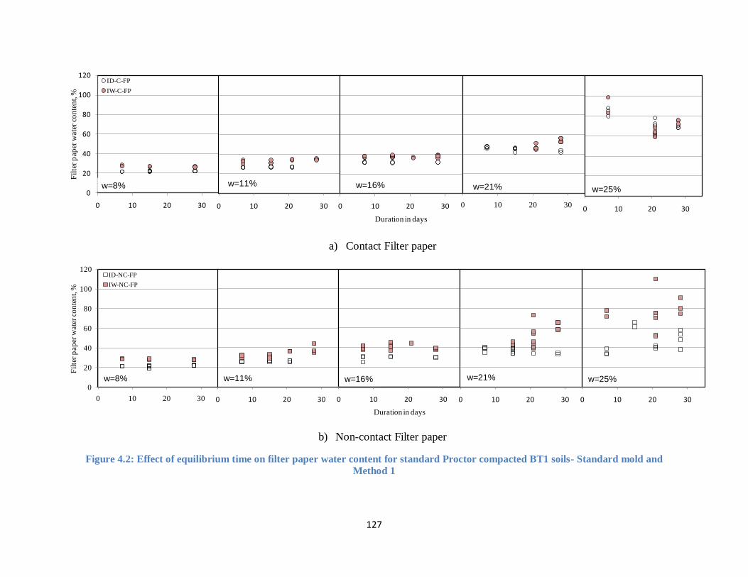
127

a) Contact Filter paper

b) Non-contact Filter paper

Figure 4.2: Effect of equilibrium time on filter paper water content for standard Proctor compacted BT1 soils- Standard mold and

Method 1

0

20

40

60

80

100

120

0 10 20 30

Fil

ter

pap

er w

ate

r co

nte

nt,

%ID-C-FP

IW-C-FP

w=8%

0 10 20 30

w=11%

0 10 20 30

Duration in days

w=16%

0 10 20 30

w=21%

0 10 20 30

w=25%

0

20

40

60

80

100

120

0 10 20 30

Fil

ter

pap

er w

ate

r co

nte

nt,

%

ID-NC-FP

IW-NC-FP

w=8%

0 10 20 30

w=11%

0 10 20 30

Duration in days

w=16%

0 10 20 30

w=21%

0 10 20 30

w=25%

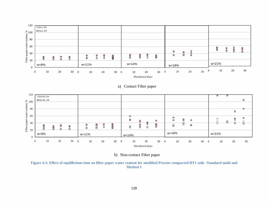
128



Figure 4.3: Effect of equilibrium time on filter paper water content for modified Proctor compacted BT1 soils- Standard mold and

Method 1

0

20

40

60

80

100

120

0 10 20 30

Fil

ter

pap

er w

ate

r co

nte

nt,

%ID-C-FP

IW-C-FP

w=8%

0 10 20 30

w=11%

0 10 20 30

Duration in days

w=14%

0 10 20 30

w=18%

0 10 20 30

w=21%

0

20

40

60

80

100

120

0 10 20 30

Fil

ter

pap

er w

ate

r co

nte

nt,

%

ID-NC-FP

IW-NC-FP

w=8%

0 10 20 30

w=11%

0 10 20 30

Duration in days

w=14%

0 10 20 30

w=18%

0 10 20 30

w=21%

129



Figure 4.4: Effect of equilibrium time on filter paper water content for standard Proctor compacted JF2 soils- Standard mold and

Method 1

0

20

40

60

80

100

120

0 10 20 30

Fil

ter

pap

er w

ate

r co

nte

nt,

%

ID-C-FP

IW-C-FP

w=9.5%

0 10 20 30

w=14%

0 10 20 30

Duration in days

w=16%

0 10 20 30

w=18%

0

20

40

60

80

100

120

0 10 20 30

Fil

ter

pap

er w

ate

r co

nte

nt,

%

ID-NC-FP

IW-NC-FP

w=9.5%

0 10 20 30

w=14%

0 10 20 30

Duration in days

w=16%

0 10 20 30

w=18%

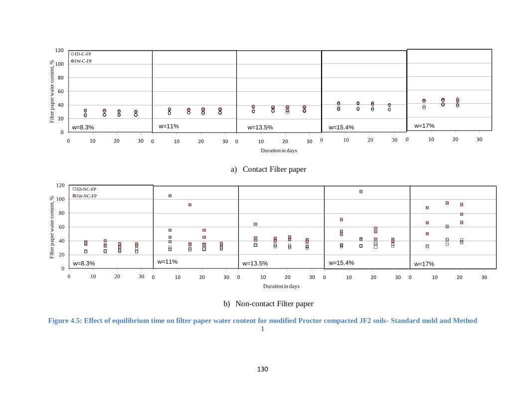
130



Figure 4.5: Effect of equilibrium time on filter paper water content for modified Proctor compacted JF2 soils- Standard mold and Method

1

0

20

40

60

80

100

120

0 10 20 30

Fil

ter

pap

er w

ate

r co

nte

nt,

%ID-C-FP

IW-C-FP

w=8.3%

0 10 20 30

w=11%

0 10 20 30

Duration in days

w=13.5%

0 10 20 30

w=15.4%

0 10 20 30

w=17%

0

20

40

60

80

100

120

0 10 20 30

Fil

ter

pap

er w

ate

r co

nte

nt,

%

ID-NC-FP

IW-NC-FP

w=8.3%

0 10 20 30

w=11%

0 10 20 30

Duration in days

w=13.5%

0 10 20 30

w=15.4%

0 10 20 30

w=17%

131

Figure 4.6: Drying pattern of 12 initially wet filter papers

Better agreement of contact and non- contact filter paper water contents is observed for the

initially dry filter papers compared to initially wet filter papers. Deviations between the contact

and non-contact filter papers’ water contents occur when the water contents exceed 47% which

coincides with the water content break in Equation 3.4. It is most likely that the non-contact filter

paper did not have sufficient time to reach equilibrium within 28 days. Further evidence is shown

by the ID-NC-FP water content being lower than the ID-C-FP water content, and the IW-NC-FP

water content being higher than the IW-C-FP water content.

0

50

100

150

200

250

300

0 4 8 12 16 20 24

Fil

ter

pap

er w

ate

r co

nte

nt,

%

Duration, h

Filter paper 1

Filter paper 2

Filter paper 3

Filter paper 4

Filter paper 5

Filter paper 6

Filter paper 7

Filter paper 8

Filter paper 9

Filter paper 10

Filter paper 11

Filter paper 12

132

a) BT1 b) BT2

c) JF2

Figure 4.7: Comparison of contact and non-contact initially dry filter papers

0

10

20

30

40

50

60

70

80

90

100

0 10 20 30 40 50 60 70 80 90 100

ID-C

-FP

wa

ter

con

ten

t,%

ID-NC-FP water content, %

Standard mold samples

Plastic mold samples

BT1 soil

1:1 line0

10

20

30

40

50

60

70

80

90

100

0 10 20 30 40 50 60 70 80 90 100

ID-C

-FP

wa

ter

con

ten

t,%




BT2 soil

1:1 line

0

10

20

30

40

50

60

70

80

90

100

0 10 20 30 40 50 60 70 80 90 100

ID-C

-FP

wa

ter

con

ten

t,%



Plastic mold samples1:1 line

JF2 soil

133

a) BT1 b) BT2

c) JF2

Figure 4.8:Comparison of contact and non-contact initially wet filter papers

4.2.3 Hysteresis

Figure 4.9 shows the hysteresis between the initially dry and initially wet filter papers in contact

and non-contact modes for the BT1, BT2 and JF2 soils. The initially wet filter papers data shown

0

10

20

30

40

50

60

70

80

90

100

0 10 20 30 40 50 60 70 80 90 100

IW-C

-FP

wa

ter

con

ten

t,%

IW-NC-FP water content, %



BT1 soil

1:1 line

0

10

20

30

40

50

60

70

80

90

100

0 10 20 30 40 50 60 70 80 90 100

IW-C

-FP

wa

ter

con

ten

t,%




BT2 soil

0

10

20

30

40

50

60

70

80

90

100

0 10 20 30 40 50 60 70 80 90 100

IW-C

-FP

wa

ter

con

ten

t,%




JF2 soil

134

in Figure 4.9 were prepared using Method 2 and the equilibration time for all the filter papers

was at least 28 days. Equivalent data for Method 1 are shown in Appendix A2.

Figure 4.9 shows that the hysteresis between the initially dry and initially wet filter papers is less

than 5% as observed by Leong et al. (2002b). The hysteresis in the non-contact filter papers for

soil BT1 and JF2 in Method 1 is higher than 5% (see Appendix A2). This is because there was

less control on the initial water content of the filter paper in Method 1 and in addition, maximum

equilibration time was 28 days. Therefore, the higher hysteresis may be due to insufficient

equilibration time for the initially wet filter paper. The non-contact filter paper for BT2 was

allowed longer duration time (up to 60 days) hence the smaller hysteresis between the initially

dry and initially wet filter papers.

Because of the hysteresis between the initially dry and initially wet filter papers, calibration

equation such as Equation 3.4 established using initially dry filter papers will underestimate the

suction of the soil if used on initially wet filter papers. To account for hysteresis, the water

contents in Equation 3.4 can be offset by -4% for initially wet filter papers as shown in Equation

4.1.

47%4)(w 4)0.0673(w4.945logψ

47%4)(w 4)0.0229(w2.909logψ

ff

ff

4.1

4.2.4 Suction measurements

The suction of the as-compacted soil specimen was measured using both contact and non-contact

filter papers. The ID-C-FP measures the matric suction of the soil specimens according to

Equation 3.4. The matric suctions of the as-compacted soil specimens are plotted against the ID-

NC-FP and the IW-NC-FP water contents for the same soil specimen in Figure 4.10. The initially

135

wet filter paper was prepared using Method 2 and equilibration time for all the filter papers was

more than 28 days.

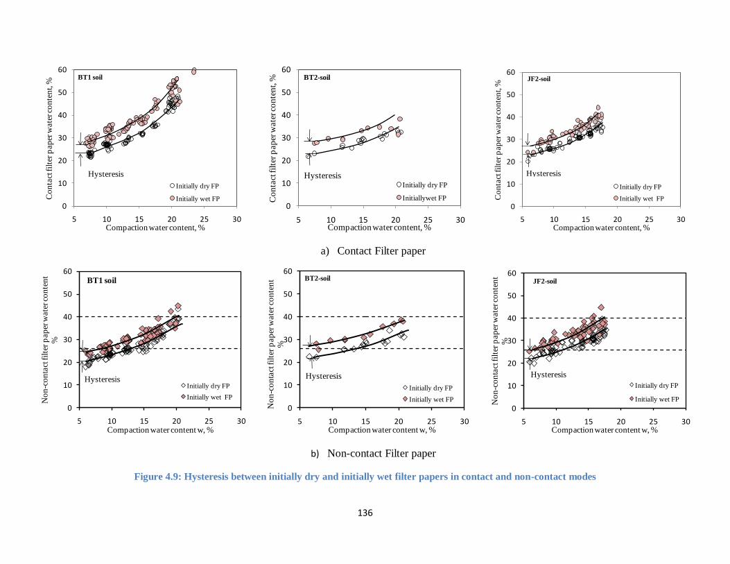
136



Figure 4.9: Hysteresis between initially dry and initially wet filter papers in contact and non-contact modes

0

10

20

30

40

50

60

5 10 15 20 25 30

Co

nta

ct fil

ter

pap

er w

ate

r co

nte

nt,

%


Initially dry FP

Initially wet FP

Hysteresis

BT1 soil

0

10

20

30

40

50

60

5 10 15 20 25 30

Co

nta

ct fil

ter

pap

er w

ate

r co

nte

nt,

%


Initially dry FP

Initiallywet FP

BT2-soil

Hysteresis

0

10

20

30

40

50

60

5 10 15 20 25 30

Co

nta

ct fil

ter

pap

er w

ate

r co

nte

nt,

%


Initially dry FP

Initially wet FP

Hysteresis

JF2-soil

0

10

20

30

40

50

60

5 10 15 20 25 30

No

n-c

on

tact

fil

ter

pap

er w

ate

r co

nte

nt

%

Compaction water content w, %

Initially dry FP

Initially wet FP

Hysteresis

BT1 soil

0

10

20

30

40

50

60

5 10 15 20 25 30

No

n-c

on

tact

fil

ter

pap

er w

ate

r co

nte

nt

%


Initially dry FP

Initially wet FP

Hysteresis

BT2-soil

0

10

20

30

40

50

60

5 10 15 20 25 30

No

n-c

on

tact

fil

ter

pap

er w

ate

r co

nte

nt

%


Initially dry FP

Initially wet FP

Hysteresis

JF2-soil

137

Best-fit lines were determined and the equations are shown in Figure 4.10 together with the

coefficient of determination R2. In addition, Equations 3.4 and 4.1 for filter paper water content

less than 47% are also plotted in Figure 4.10 for comparison. Good agreement can be found

between the best-fit lines, and Equations 3.4 and 4.1, with the BT soil data showing better

agreement than the JF soil data. This indicates that the ID-NC-FP and IW-NC-FP can be

interpreted using the matric suction calibration curve equations, Equations 3.4 and 4.1,

respectively, for filter paper water content less than 47%.

a) BT1 b) BT2

b) JF2

Figure 4.10: Suction calibration curves for initially dry and initially wet filter paper in non contact

mode

Initially dry filter paper

log = 4.8895- 0.0660 wf

R² = 0.9292

Initially wet filter paper

log = 4.2183 - 0.0691wf

R² = 0.8454

10

100

1000

10000

0 10 20 30 40 50 60

Su

ctio

n, k

Pa

Filter paper water content, %

ID-NC-FP

IW-NC-FP

26 47

BT1 soil

Eq. 4.1

Eq. 3.4


log = 4.7779- 0.0608 wf

R² = 0.846


log = 4.7417 - 0.0478wf

R² = 0.749

10

100

1000

10000

0 10 20 30 40 50 60

Su

ctio

n, k

Pa


ID-NC-FP

IW-NC-FP

26 47

BT2 soil

Eq. 4.1

Eq. 3.4


log = 4.7185- 0.0617 wf

R² = 0.7736


log = 4.8199 - 0.0565wf

R² = 0.7269

10

100

1000

10000

0 10 20 30 40 50 60

Su

ctio

n, k

Pa


ID-NC-FP

IW-NC-FP

26 47

JF2 soil

Eq. 4.1

Eq. 3.4

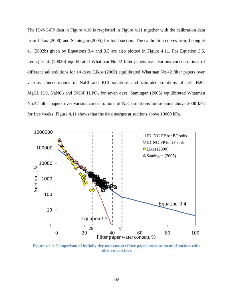
138

The ID-NC-FP data in Figure 4.10 is re-plotted in Figure 4.11 together with the calibration data

from Likos (2000) and Samingan (2005) for total suction. The calibration curves from Leong et

al. (2002b) given by Equations 3.4 and 3.5 are also plotted in Figure 4.11. For Equation 3.5,

Leong et al. (2002b) equilibrated Whatman No.42 filter papers over various concentrations of

different salt solutions for 14 days. Likos (2000) equilibrated Whatman No.42 filter papers over

various concentrations of NaCl and KCl solutions and saturated solutions of LiCl.H20,

MgCl2.H20, NaNO2 and (NH4).H2PO4 for seven days. Samingan (2005) equilibrated Whatman

No.42 filter papers over various concentrations of NaCl solutions for suctions above 2000 kPa

for five weeks. Figure 4.11 shows that the data merges at suctions above 10000 kPa.

Figure 4.11: Comparison of initially dry non-contact filter paper measurement of suction with

other researchers

1

10

100

1000

10000

100000

1000000

0 20 40 60 80 100

Su

ctio

n, k

Pa


ID- NC-FP for BT soils

ID-NC-FP for JF soils

Likos (2000)

Samingan (2005)

26 47

Equation 3.5

Equation 3.4

139

For suctions less than 10000 kPa, Likos (2000)’s data starts to diverge from the rest probably due

to insufficient equilibration time. Most of the ID-NC-FP data from the present study seems to

straddle between the calibration curves given by Equations 3.4 and 3.5 indicating that

equilibration time of 28 to 60 days may not be sufficient for some of the ID-NC-FP. This

suggests Marinho and Oliveira (2006) is correct in explaining equilibration time being the cause

of the difference between the total and matric suction calibration curves but it is difficult to use

the matric suction calibration curve for the non-contact filter paper as equilibrium may not be

achieved within a reasonable time. This suggests that the non-contact filter paper is only suitable

for use in the high suction range. The present data indicates that the suction range for non-

contact filter paper should be above 1000 kPa.

Total suction of the soil specimens were also measured independently using the CMDP

technique. The total suction measured by WP4C, ID-NC-FP and ID-C-FP are plotted against

compaction water content in Figure 4.12.

The ID-NC-FP was interpreted using both Equations 3.4 and 3.5. The ID-C-FP was interpreted

using Equation 3.4. Generally, there is good agreement for suctions above 1000 kPa. Below 1000

kPa suction, the suction given by the WP4C lies in between the suctions given by Equations 3.4

and 3.5 for the ID-NC-FP. The suctions given by Equation 3.4 for ID-NC-FP are higher than the

suctions given by WP4C and can be attributed to insufficient equilibrium time. The large

divergence of the suctions given by Equation 3.5 for the ID-NC-FP and the suctions given by

WP4C is due to Equation 3.5 diverging from Equation 3.4 below 1000 kPa. Although ASTM

D6836-16 does not recommend the CMDP technique to measure suctions below 1000 kPa, there

140

seems to be good agreement between the suctions given by Equation 3.4 for the ID-C-FP and the

suctions given by WP4C for suctions below 1000 kPa.

a) BT1 b) BT2

c) JF2

Figure 4.12: Comparison of suction measurements by initially dry non-contact filter paper and

chilled mirror dewpoint technique

1

10

100

1000

10000

5 10 15 20 25

Su

ctio

n, k

Pa

Compaction water content,%

ID-NC-FP: Equation 3.4


ID-C-FP: Equation 3.4

WP4C

BT1 soil

1

10

100

1000

10000

5 10 15 20 25S

uct

ion

, kP

a




ID-C-FP: Equation 3.4

WP4C

BT2 soil

1

10

100

1000

10000

5 10 15 20 25

Su

ctio

n, k

Pa


ID-NC-FP: Eq. 3.4

ID-NC-FP: Eq. 3.5

ID-C-FP: Eq. 3.4

WP4C

JF2 soil

141

4.2.5 Variability of filter papers

Deka et al. (1995) and Marinho and Oliveira (2006) investigated the inherent variability of the

Whatman No.42 filter papers and noted that different batches of filter papers may have different

characteristics causing differences in the calibration curves between batches. Bulut and Wray

(2005) also suggested a change in absorption characteristics of the Whatman No. 42 filterpaper

under the application of a pressure.

The variability of Whatman No. 42 filter papers in terms of weight after oven drying was

examined for 48 unused filter papers and 1716 used filter papers. The used filter papers were

separated into those used in contact (844 filter papers) and non-contact (872 filter papers) modes.

According to the manufacturer’s specifications, the Whatman No. 42 filter paper weighs

100g/m2. Hence, for a filter paper that is 42.5 mm in diameter, the mean weight is expected to be

0.142g. Accounting for the initial moisture content (6.6%) of the filter paper, the expected mean

weight is 0.133g. The weight distributions of the used and unused filter papers shown in Figure

4.13 have a normal distribution. The unused filter papers have a narrower weight distribution

from 0.13 to 0.14g with peak at 0.135g. The used filter papers have a wider weight distribution

with the non-contact filter papers showing a weight distribution from 0.115 to 0.145g with a

peak at 0.13g and the contact filter papers showing a weight distribution from 0.11 to 0.15g with

a peak at 0.135g.

Hence, some permanent changes occurred in the filter paper after use and the change is slightly

more for the contact filter paper. There is little evidence that the contact filter paper becomes

contaminated during use hence the use of sacrificial filter papers recommended by ASTM

D5298-16 seems unnecessary.

142

Figure 4.13: Weight distribution of dried filter papers before and after use

4.2.6 Summary

In this study, the efficacy of using initially dry and initially wet Whatman No. 42 filter papers for

suction measurement of dynamically compacted soils was evaluated using more than 1700 pieces

of filter papers. Suction measurements were performed on soils compacted at various water

contents using both the standard and modified Proctor efforts. The initially wet filter papers were

prepared using two methods. Important conclusions from this study are:

1) It is easier to handle initially dry filter papers compared to initially wet filter papers. When

filter papers are wetted, there is a likelihood of altering their characteristics and hence

affecting their performance in suction measurement.

2) When using initially wet filter paper, pre-wetting to a specific moisture content (Method 2)

will give better outcome than not controlling its moisture content.

0%

10%

20%

30%

40%

50%

60%

70%

80%

0.1

05

0.1

10

0.1

15

0.1

20

0.1

25

0.1

30

0.1

35

0.1

40

0.1

45

0.1

50

0.1

55

0.1

60

0.1

65

Fre

qu

ency

Mass, g

Before use - oven dried

Non-Contact FP

Contact FP

143

3) An initially wet filter paper may require even longer equilibrium time compared to an

initially dry filter paper. When used in the non-contact mode, the equilibrium time depends

on the air space above the soil specimen, the suction of the soil and the initial moisture

condition of the filter paper.

4) Hysteresis between initially dry and initially wet filter paper can be accounted for by

applying an offset on the water content in the initially dry filter paper calibration curve.

The study showed that the offset is about -4% for the Whatman No. 42 filter paper.

5) Comparison of the weight distributions of used and unused filter papers show that the used

filter papers have a slightly wider weight distribution than the unused filter papers. There is

negligible difference in weight distributions between the contact and non-contact filter

papers indicating that contamination of filter paper is not an issue and hence, there may not

be a need to use sacrificial filter papers in the contact method to prevent contamination of

the filter paper.

6) Good agreement was found between the suctions measured using the WP4C and the

initially dry contact filter paper.

7) For both initially dry and initial wet filter papers, the contact mode gives more reliable

suction measurement than the non-contact mode.

8) The non-contact filter paper is suitable only for the high suction range, above 1000 kPa

whereas the contact filter paper is suitable for both the high and low suction ranges.

4.3 Soil-water characteristic curves of compacted soils

Soil-water characteristics curves (SWCC) of compacted soils have been studied by other

researchers. Factors influencing the SWCC studied includes:

1) Initial compaction water content e.g.Vanapalli et al. (1999).

144

2) Initial dry density e.g. Salager et al. (2010), Zhou et al. (2012), Mirzaii and Yasrobi

(2012), and Wijaya and Leong (2017).

3) Influence of stress history e.g. Vanapalli et al. (1999) and Marinho (2005).

These factors are further explored in this study. Both the SWCC-w and SWCC-S for the soil

specimens were studied. Only the drying SWCCs have been studied in this thesis. The as-

compacted characteristics of the soil specimens are presented in Tables 4.1 to 4.4.

Table 4.1: Average properties for BT1 specimens measured for SWCC

BT1- soil dry densities, Mg/m3

BT1-

PL/ASTM Compacted at w% PL specimen

ASTM

specimen

STD10 dry of optimum 10 1.64 1.64


STD16 optimum 16 1.68 1.69

STD18 wet of optimum 18 1.69 1.67


MDF7 dry of optimum 7 1.80 1.79


MDF13 optimum 13 1.83 1.86

MDF16 wet of optimum 16 1.81 1.82


145

Table 4.2: Average properties for BT2 specimens measured for SWCC

dry densities, Mg/m3

BT2-

PL/ASTM Compacted at w% PL specimen

ASTM

specimen



STD19.5 wet of optimum 19.5 1.68 1.70



MDF11 dry of optimum 11 - 1.86

MDF13 optimum 13 - 1.88



Table 4.3: Average properties of JF1 specimens measured for SWCC

JF1-PL Compacted at w% dry density,

Mg/m3

STD13 dry of optimum 13 1.59

STD18 optimum 18 1.63

STD22 wet of optimum 22 1.63

MDF9 dry of optimum 9 1.74

MDF15 optimum 15 1.78

MDF19.5 wet of optimum 19.5 1.74

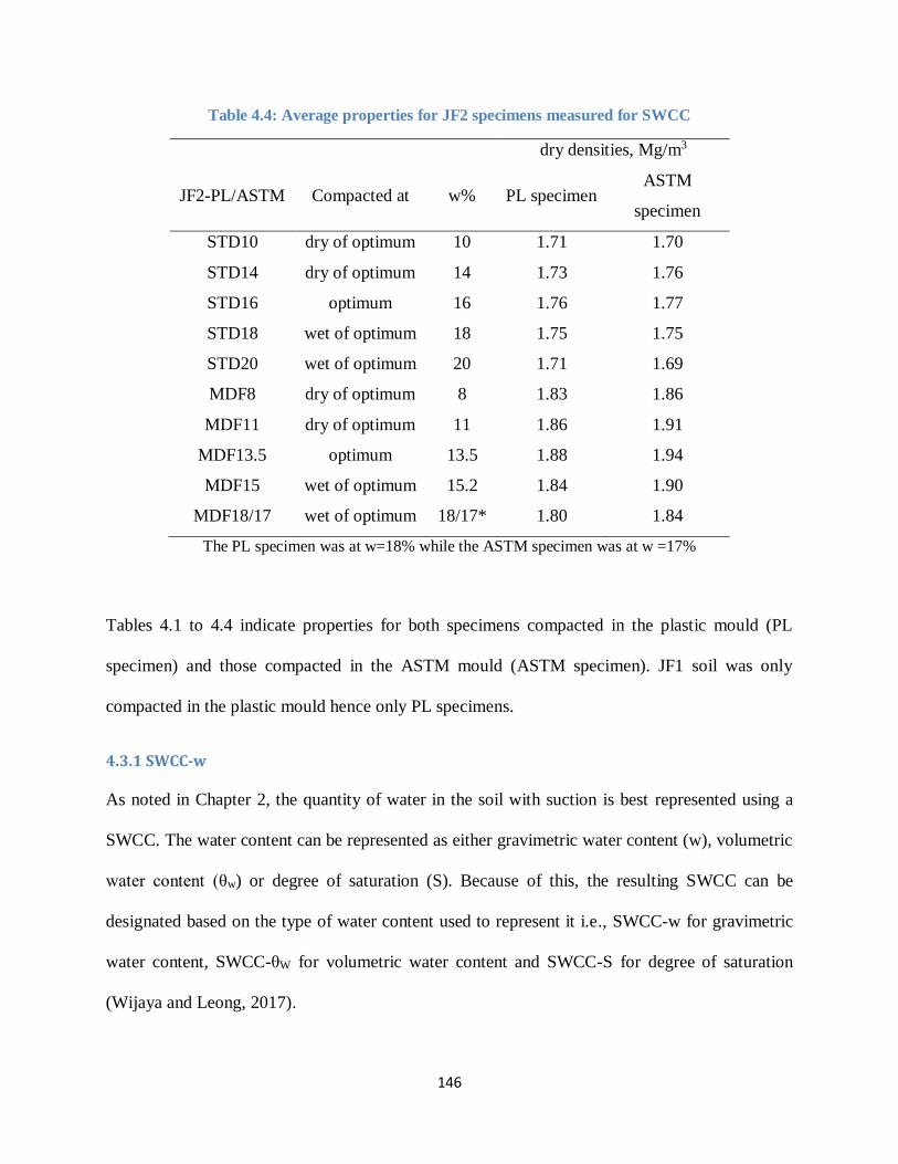
146

Table 4.4: Average properties for JF2 specimens measured for SWCC

dry densities, Mg/m3

JF2-PL/ASTM Compacted at w% PL specimen ASTM

specimen



STD16 optimum 16 1.76 1.77





MDF13.5 optimum 13.5 1.88 1.94

MDF15 wet of optimum 15.2 1.84 1.90

MDF18/17 wet of optimum 18/17* 1.80 1.84

The PL specimen was at w=18% while the ASTM specimen was at w =17%

Tables 4.1 to 4.4 indicate properties for both specimens compacted in the plastic mould (PL

specimen) and those compacted in the ASTM mould (ASTM specimen). JF1 soil was only

compacted in the plastic mould hence only PL specimens.

4.3.1 SWCC-w

As noted in Chapter 2, the quantity of water in the soil with suction is best represented using a

SWCC. The water content can be represented as either gravimetric water content (w), volumetric

water content (θw) or degree of saturation (S). Because of this, the resulting SWCC can be

designated based on the type of water content used to represent it i.e., SWCC-w for gravimetric

water content, SWCC-θW for volumetric water content and SWCC-S for degree of saturation

(Wijaya and Leong, 2017).

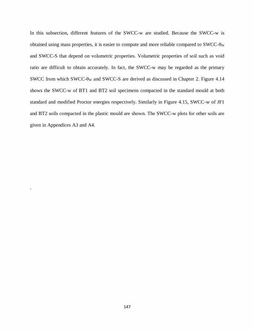
147

In this subsection, different features of the SWCC-w are studied. Because the SWCC-w is

obtained using mass properties, it is easier to compute and more reliable compared to SWCC-θW

and SWCC-S that depend on volumetric properties. Volumetric properties of soil such as void

ratio are difficult to obtain accurately. In fact, the SWCC-w may be regarded as the primary

SWCC from which SWCC-θW and SWCC-S are derived as discussed in Chapter 2. Figure 4.14

shows the SWCC-w of BT1 and BT2 soil specimens compacted in the standard mould at both

standard and modified Proctor energies respectively. Similarly in Figure 4.15, SWCC-w of JF1

and BT2 soils compacted in the plastic mould are shown. The SWCC-w plots for other soils are

given in Appendices A3 and A4.

.

148

(a) BT1

(b) BT2

Figure 4.14: SWCC-w for samples compacted in the standard mould

0

0.1

0.2

0.3

0.4

1 10 100 1000 10000 100000 1000000

Gra

vim

etri

c w

ate

r co

nte

nt

Suction, kPa

BT1-MDF-ASTM7BT1-MDF-ASTM10BT1-MDF-ASTM13BT1-MDF-ASTM16BT1-MDF-ASTM18BT1-STD-ASTM10BT1-STD-ASTM13BT1-STD-ASTM16BT1-STD-ASTM18BT1-STD-ASTM20

BT1 soil

0

0.1

0.2

0.3

0.4

1 10 100 1000 10000 100000 1000000

Gra

vim

etri

c w

ate

r co

nte

nt

Suction, kPa

BT2-MDF-ASTM8

BT2-MDF-ASTM11

BT2-MDF-ASTM13

BT2-MDF-ASTM15

BT2-MDF-ASTM16

BT2-STD-ASTM13

BT2-STD-ASTM16

BT2-STD-ASTM19.5

BT2-STD-ASTM22

BT2 soil

149

(a) JF1

(b) BT2

Figure 4.15: SWCC-w for specimens compacted in the plastic mould

Wijaya and Leong (2017) note that density can be modeled as either saturated water content wsat,

void ratio e, or relative density. In Figures 4.14 and 4.15, as well as figures in Appendices A3

0

0.1

0.2

0.3

0.4

1 10 100 1000 10000 100000 1000000

Gra

vim

etri

c w

ate

r co

nte

nt

Suction, kPa

JF1-MDF-PL9.5

JF1-MDF-PL15

JF1-MDF-PL19.5

JF1-STD-PL13

JF1-STD-PL18

JF1-STD-PL22

JF1 soil

0

0.1

0.2

0.3

0.4

1 10 100 1000 10000 100000 1000000

Gra

vim

etri

c w

ate

r co

nte

nt

Suction, kPa

BT2-MDF-PL8

BT2-MDF-PL15

BT2-MDF-PL16

BT2-STD-PL13

BT2-STD-PL16

BT2-STD-PL19.5

BT2-STD-PL22

BT2 soil

150

and, the effect of density is represented by saturated gravimetric water content, wsat. It is

observed that initially the SWCCs show clear differences owing to differences in wsat, however

as suction increases, the SWCCs converge or near converge into a single curve which Wijaya

and Leong (2017) refers to as the virgin drying line.

The soil specimens compacted at standard Proctor effort using the standard ASTM mould

generally show a narrower band in their SWCCs compared to those compacted at modified

Proctor effort (Appendix A3). This indicates that the soil specimens compacted at standard

Proctor effort have a more uniform pore size distribution although it is expected that soil

specimens compacted at a higher compaction effort should have a more uniform pore size

distribution. However, the soil specimens compacted in the plastic mould behaved as expected

(Appendix A4).

It is difficult to control the initial dry density of the compacted soil specimens precisely. The

error will show up in the initial part of the SWCC-w through wsat. Apart from BT2 soil

specimens, most of the SWCC-w tend to converge into one curve beyond a suction of 1000 kPa.

The SWCC-w of BT2 soil specimens whether compacted in the standard mould or plastic mould

tend to converge much slower than the rest of the soil sets.

The SWCC-w can also be represented as plots of normalised gravimetric water content against

soil suction. The gravimetric water content is normalised by dividing gravimetric water content

with the saturated gravimetric water content i.e., w/wsat. For soils with negligible volume change

during drying, normalised gravimetric water content is equivalent to degree of saturation

(Fredlund et al., 2012). For illustration, Figure 4.16 shows normalized SWCC-w for BT1 and

JF2 soil specimens compacted in the standard mould at both standard and modified Proctor

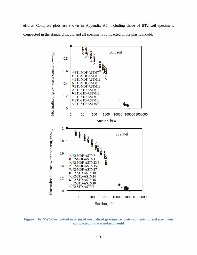
151

efforts. Complete plots are shown in Appendix A5, including those of BT2 soil specimens

compacted in the standard mould and all specimens compacted in the plastic mould.

Figure 4.16: SWCC-w plotted in terms of normalised gravimetric water contents for soil specimens

compacted in the standard mould

0

0.2

0.4

0.6

0.8

1

1 10 100 1000 10000 1000001000000No

rmali

sed

gra

v. w

ate

r co

nte

nt, w

/wsat

Suction, kPa

BT1-MDF-ASTM7BT1-MDF-ASTM10BT1-MDF-ASTM13BT1-MDF-ASTM16BT1-MDF-ASTM18BT1-STD-ASTM10BT1-STD-ASTM13BT1-STD-ASTM16BT1-STD-ASTM18BT1-STD-ASTM20

BT1 soil

0

0.2

0.4

0.6

0.8

1

1 10 100 1000 10000 100000 1000000

No

rmali

sed

G

rav. w

ate

r co

nte

nt,

w/w

sat

Suction, kPa

JF2-MDF-ASTM8JF2-MDF-ASTM11JF2-MDF-ASTM13.5JF2-MDF-ASTM15JF2-MDF-ASTM17JF2-STD-ASTM10JF2-STD-ASTM14JF2-STD-ASTM16JF2-STD-ASTM18JF2-STD-ASTM21

JF2 soil

152

From Figure 4.16 and Appendix A5 it is generally observed that SWCCs of specimens

compacted at modified Proctor effort have gentler slopes than those at standard Proctor effort.

Specimens compacted at the same compaction effort show that SWCC-w of specimens

compacted wet of optimum have gentler slopes than those compacted dry of optimum.

The slope of the SWCC-w is a reflection of the soil structure. Samples compacted wet of

optimum have a dispersed uniform structure and their SWCCs are generally controlled by the

microstructure (Vanapalli et al., 1999). In addition, specimens compacted at modified Proctor

effort have more oriented (dispersed) structures than those compacted at standard Proctor effort

(Holtz and Kovacs, 1981).The dispersed/ oriented structure implies a pore network that is

disconnected and more uniform, hence a more gradual desaturation process reflected through the

gentle slope of the SWCCs.

4.3.2 SWCC-S

The SWCC-S is the only SWCC that should be used to determine the air entry value (AEV) of a

soil that undergoes volume changes on drying (Fredlund et al., 2012). In order to establish

SWCC-S, volume measurements of the soil are required hence very often the SWCC-S is

derived from SWCC-w using a soil shrinkage curve (Wijaya and Leong, 2017). The shrinkage

curve represents the volume changes of the soil as it dries and is very often plotted as a

relationship between void ratio and gravimetric water content. In this study, volume

measurements of the specimens were taken as they dried during the SWCC tests in order to

determine their shrinkage curves. Figure 4.17 shows typical shrinkage curves for specimens

compacted at optimum water content for the BT1 and JF2 soils. The data was fitted using

153

a) BT1

b) JF2

Figure 4.17: Typical shrinkage curves

Leong and Wijaya (2015)’s universal shrinkage equation. It is observed that the samples

compacted at modified Proctor have a smaller emin compared to those compacted at standard

Proctor.

0

0.2

0.4

0.6

0.8

1

1.2

0 0.1 0.2 0.3 0.4 0.5 0.6

Vo

id r

ati

o

Moisture content

BT1-MDF-PL13

BT1-STD-PL16

BT1 soil

0

0.2

0.4

0.6

0.8

1

1.2

0 0.1 0.2 0.3 0.4 0.5 0.6

Vo

id r

ati

o

Moisture content

BT1-MDF-ASTM13

BT1-STD-ASTM16

0

0.2

0.4

0.6

0.8

1

1.2

0 0.1 0.2 0.3 0.4 0.5 0.6

Vo

id r

ati

o

Moisture content

JF2-STD-PL16

JF2-MDF-PL13.5

0

0.2

0.4

0.6

0.8

1

1.2

0 0.1 0.2 0.3 0.4 0.5 0.6

Vo

id r

ati

o

Moisture content

JF2-STD-ASTM16

JF2-MDF-ASTM13.5

154

4.3.2.1 Effect of compaction water content on SWCC-S

As discussed in Chapter 3, compaction water content influences the soil structure with specimens

compacted dry of optimum reportedly showing a flocculated soil structure which is further

characterized by a dual porosity (Sridharan et al., 1971; Ahmed et al., 1974; Delage et al., 1996).

The wet of optimum compacted specimens on the other hand are characterized by a dispersed

structure and a unimodal pore size distribution.

Figure 4.18 and 4.19 show typical SWCC-S for JF2 soil specimens compacted in the plastic and

the standard moulds, respectively. The SWCC-S data in Figures 4.18 and 4.19 were curve fitted

with Fredlund and Xing (1994) equation. This equation was recommended by Leong and

Rahardjo (1997b) as the best of all the SWCC equations commonly used in curve fitting

unimodal SWCC data. From Figures 4.18 and 4.19, the wet of optimum specimens have higher

AEVs, followed by the specimens compacted at optimum water content and finally the dry of

optimum specimens. According to Vanapalli et al. (1999), specimens compacted at dry of

optimum have less resistance to de-saturation owing to large voids between the clods which

constitute the macrostructure. The macrostructure controls the initial de-saturation process for

the specimens compacted dry of optimum (Vanapalli et al., 1999; Marinho, 2005) which

facilitates de-saturation at low suction levels. On the other hand, specimens compacted wet of

optimum have a pore network that is not interconnected resulting from a dispersed structure.

This ensures higher water storage capacity for soils compacted wet of optimum and greater

resistance to de-saturation hence the need for higher suctions for de-saturation to commence

(Vanapalli et al., 1999).

Figure 4.18 also shows that beyond the AEV, the wet of optimum specimens compacted in the

plastic mould de-saturate faster than the specimens compacted at optimum and dry of optimum

155

water contents. This is reflected by a steeper slope in the SWCC-S. Hence, the slope of the

SWCC-S reflects the pore size distribution of the specimen where a steeper slope represents a

more uniform pore size distribution. Figure 4.22 shows variation of AEV with dry density of the

compacted specimens for BT1 and BT2 both sets compacted using the standard ASTM mould.

The specimens compacted wet of optimum show higher AEV than those dry of optimum for the

reasons presented above. The specimens at the optimum density seem to lie in between. Similar

observations have been reported by Vanapalli et.al, (1999). Although it is expected that the

AEVs of wet of optimum specimens are supposed to be less sensitive to dry density than those

on the dry of optimum, both BT1 and BT2 show almost similar sensitivities

4.3.2.2 Effect of compaction effort on SWCC-S

Figures 4.20 and 4.21 presents the SWCC-S of BT1 soil specimens compacted in the plastic and

standard moulds, respectively. The SWCC-S have been categorized according to initial

compaction water content of the soil specimens i.e., either wet of optimum or dry of optimum.

The SWCC-S for specimens compacted at standard and modified Proctor efforts are combined in

each set.

156

a) Specimens compacted at standard Proctor effort

b) Specimens compacted at modified Proctor effort

Figure 4.18:SWCC-S for JF2 soil specimens compacted at standard and modified Proctor efforts in

the plastic mould

0

0.2

0.4

0.6

0.8

1

1 10 100 1000 10000 100000 1000000

Deg

ree

of

Satu

rati

on

Suction, kPa

JF2-STD-PL10 (dry of otimum)

JF2-STD-PL16 (optimum)

JF2-STD-PL21 (wet of optimum)

0

0.2

0.4

0.6

0.8

1

1 10 100 1000 10000 100000 1000000

Deg

ree

of

Satu

rati

on

Suction, kPa

JF2-MDF-PL8 (dry of optimum)

JF2-MDF-PL13.5 (optimum)

JF2-MDF-PL17 (wet of optimum)

0

0.2

0.4

0.6

0.8

1

1101001000100001000001000000

Deg

ree

of

Satu

rati

on

Suction, kPa

FX model-fitted to wet of optimum SWCC data

FX model fitted to dry of optimum SWCC data

FX model fitted to optimum SWCC data

LEGEND:

157

a) Specimens compacted at standard Proctor effort

b) Specimens compacted at modified Proctor effort

Figure 4.19: SWCC-S for JF2 soil specimens compacted at standard and modified Proctor efforts in

the standard mould

0

0.2

0.4

0.6

0.8

1

1 10 100 1000 10000 100000 1000000

Deg

ree

of

Satu

rati

on

Suction, kPa

JF2-STD-ASTM10 (dry of optimum)

JF2-STD-ASTM16 (optimum)

JF2-STD-ASTM21 (wet of optimum)

0

0.2

0.4

0.6

0.8

1

1 10 100 1000 10000 100000 1000000

Deg

ree

of

Satu

rati

on

Suction, kPa

JF2-MDF-ASTM8 (dry of optimum)

JF2-MDF-ASTM13.5 (optimum)

JF2-MDF-ASTM17 (wet of optimum)

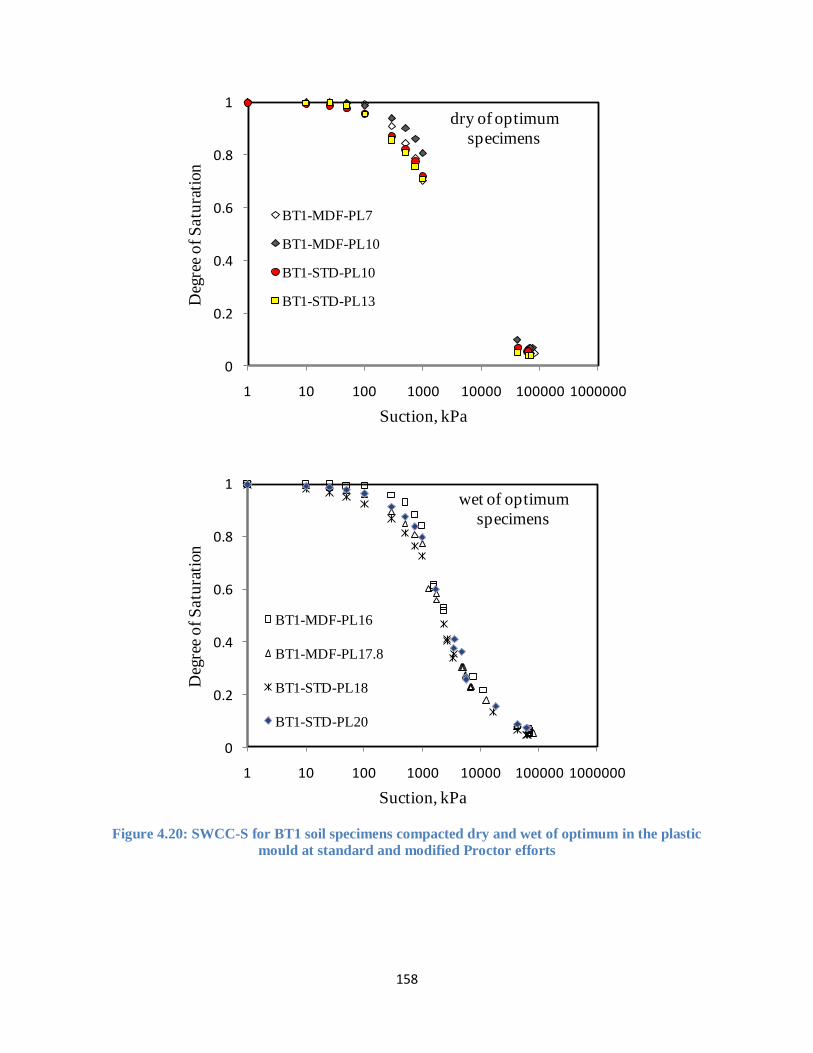
158

Figure 4.20: SWCC-S for BT1 soil specimens compacted dry and wet of optimum in the plastic

mould at standard and modified Proctor efforts

0

0.2

0.4

0.6

0.8

1

1 10 100 1000 10000 100000 1000000

Deg

ree

of

Satu

rati

on

Suction, kPa

BT1-MDF-PL7

BT1-MDF-PL10

BT1-STD-PL10

BT1-STD-PL13

dry of optimum

specimens

0

0.2

0.4

0.6

0.8

1

1 10 100 1000 10000 100000 1000000

Deg

ree

of

Satu

rati

on

Suction, kPa

BT1-MDF-PL16

BT1-MDF-PL17.8

BT1-STD-PL18

BT1-STD-PL20

wet of optimum

specimens

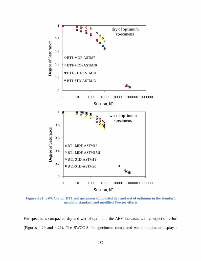
159

Figure 4.21: SWCC-S for BT1 soil specimens compacted dry and wet of optimum in the standard

mould at standard and modified Proctor efforts

For specimens compacted dry and wet of optimum, the AEV increases with compaction effort

(Figures 4.20 and 4.21). The SWCC-S for specimens compacted wet of optimum display a

0

0.2

0.4

0.6

0.8

1

1 10 100 1000 10000 100000 1000000

Deg

ree

of

Satu

rati

on

Suction, kPa

BT1-MDF-ASTM7

BT1-MDF-ASTM10

BT1-STD-ASTM10

BT1-STD-ASTM13

dry of optimum

specimens

0

0.2

0.4

0.6

0.8

1

1 10 100 1000 10000 100000 1000000

Deg

ree

of

Satu

rati

on

Suction, kPa

BT1-MDF-ASTM16

BT1-MDF-ASTM17.8

BT1-STD-ASTM18

BT1-STD-ASTM20

wet of optimum

specimens

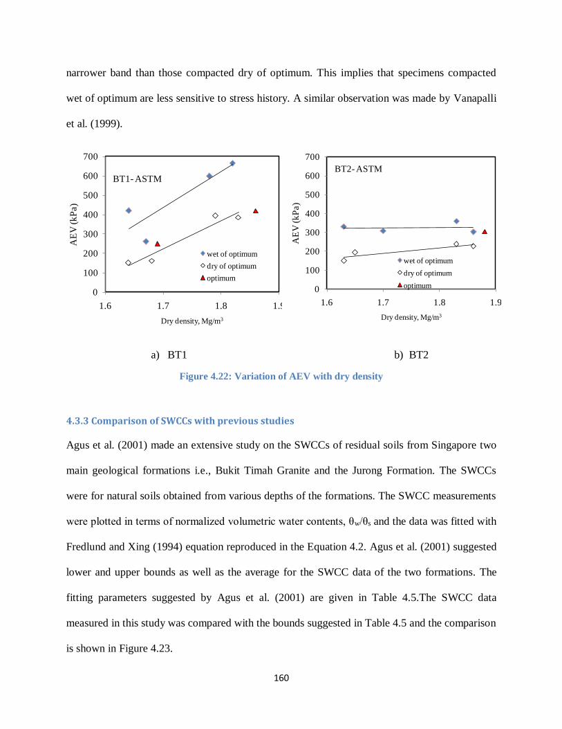
160

narrower band than those compacted dry of optimum. This implies that specimens compacted

wet of optimum are less sensitive to stress history. A similar observation was made by Vanapalli

et al. (1999).

a) BT1 b) BT2

Figure 4.22: Variation of AEV with dry density

4.3.3 Comparison of SWCCs with previous studies

Agus et al. (2001) made an extensive study on the SWCCs of residual soils from Singapore two

main geological formations i.e., Bukit Timah Granite and the Jurong Formation. The SWCCs

were for natural soils obtained from various depths of the formations. The SWCC measurements

were plotted in terms of normalized volumetric water contents, θw/θs and the data was fitted with

Fredlund and Xing (1994) equation reproduced in the Equation 4.2. Agus et al. (2001) suggested

lower and upper bounds as well as the average for the SWCC data of the two formations. The

fitting parameters suggested by Agus et al. (2001) are given in Table 4.5.The SWCC data

measured in this study was compared with the bounds suggested in Table 4.5 and the comparison

is shown in Figure 4.23.

0

100

200

300

400

500

600

700

1.6 1.7 1.8 1.9

AE

V (k

Pa)

Dry density, Mg/m3

wet of optimum

dry of optimum

optimum

BT1- ASTM

0

100

200

300

400

500

600

700

1.6 1.7 1.8 1.9A

EV

(k

Pa)

Dry density, Mg/m3

wet of optimum

dry of optimum

optimum

BT2- ASTM

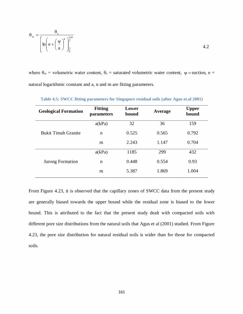
161

mn

s

w

a

ψeln

θθ

4.2

where θw = volumetric water content, θs = saturated volumetric water content, ψ suction, e =

natural logarithmic constant and a, n and m are fitting parameters.

Table 4.5: SWCC fitting parameters for Singapore residual soils (after Agus et.al 2001)

Geological Formation Fitting

parameters

Lower

bound Average

Upper

bound

a(kPa) 32 36 159

Bukit Timah Granite n 0.525 0.565 0.792

m 2.243 1.147 0.704

a(kPa) 1185 299 432

Jurong Formation n 0.448 0.554 0.93

m 5.387 1.869 1.004

From Figure 4.23, it is observed that the capillary zones of SWCC data from the present study

are generally biased towards the upper bound while the residual zone is biased to the lower

bound. This is attributed to the fact that the present study dealt with compacted soils with

different pore size distributions from the natural soils that Agus et al (2001) studied. From Figure

4.23, the pore size distribution for natural residual soils is wider than for those for compacted

soils.

162

a) Bukit Timah Granite

b) Jurong Formation

Figure 4.23: Comparison of SWCC data with SWCC envelopes suggested by Agus et al.

(2001)

0

0.2

0.4

0.6

0.8

1

1 10 100 1000 10000 100000 1000000

No

rmali

sed

vo

lum

etri

c w

ate

r co

nte

nt,

θw/θ

s

Suction, kPa

Upper bound (Agus et.al, 2001)

Average (Agus et.al, 2001)

Lower bound (Agus et.al, 2001)

BT1 soil sets (present study)

BT2 soil sets (present study)

0

0.2

0.4

0.6

0.8

1

1 10 100 1000 10000 100000 1000000

No

rmali

sed

vo

lum

etri

c w

ate

r co

nte

nt,

θw/θ

s

Suction, kPa

Upper bound (Agus et.al, 2001)

Average (Agus et.al, 2001)

Lower bound (Agus et.al, 2001)

JF2 soil sets (present study)

JF1 soil sets (present study)

163

4.4 Comparison of suctions from filter paper method and SWCC

This section presents the suctions of the as-compacted soil specimens measured using the filter

paper technique as well as the suctions estimated from the SWCC of the same compacted soils.

The comparison is shown in Figure 4.24.

Figure 4.24: Comparison of suctions measured using filter paper technique and suctions estimated

from the SWCC

It should be emphasized that the filter paper method measured the suctions of as-compacted soils

and each specimen compacted at a particular water content is considered to be a “different soil”

as discussed in Chapter 3. Each of the compacted soil specimens has a different SWCC.

From Figure 4.24, it is observed that suctions from the filter paper method compares very well

with suctions estimated from the SWCCs in the lower suction range, especially below 1000 kPa.

In the high suction range, suctions from the SWCC are higher than those from the filter paper

0

2000

4000

6000

8000

0 2000 4000 6000 8000

Su

ctio

n e

stim

ated

fro

m F

P, k

Pa

Suction estimated from SWCC, kPa

line 1:1

164

method. In the low suction range, the water phase in the soil specimen is continuous and hence it

is easier to measure matric suction more accurately using the contact filter paper.

The present study did not have many SWCC measurements above 1000kPa which may have

influenced the bias in the data shown in Figure 4.24.


This chapter presented two main issues: suction measurements using the filter paper method and

SWCCs. As earlier emphasized, the suction measurements using the filter paper were done on

as-compacted soil specimens and each specimen compacted at a particular water content and

compaction effort should be regarded as a “different” soil with its own SWCC.

The main findings in this chapter are summarized below:

1) The filter paper technique is still a very valuable technique in suction measurement if a

strict protocol is observed because the filter paper method can measure a wide range of

suctions and is affordable. The initially dry filter paper is preferred to the initially wet

filter paper. It is easier to handle initially dry filter papers compared to initially wet filter

papers. When filter papers are wetted, there is a likelihood of altering their characteristics

and hence affecting their performance in suction measurement. When using initially wet

filter paper, pre-wetting to a specific moisture content (Method 2) will give better

outcome than not controlling its moisture content.

2) An initially wet filter paper may require even longer equilibrium time compared to an

initially dry filter paper. When used in the non-contact mode, the equilibrium time

depends on the air space above the soil specimen, the suction of the soil and the initial

165

moisture condition of the filter paper. The hypothesis that an initially wet filter paper may

reduce equilibration time was not supported by study.

3) Hysteresis between initially dry and initially wet filter paper can be accounted for by

applying an offset on the water content in the initially dry filter paper calibration curve.

The study showed that the offset is about -4% for the Whatman No. 42 filter paper.

4) Comparison of the weight distributions of used and unused filter papers show that the

used filter papers have a slightly wider weight distribution than the unused filter papers.

There is negligible difference in weight distributions between the contact and non-contact

filter papers indicating that contamination of filter paper is not an issue and hence, there

may not be a need to use sacrificial filter papers in the contact method to prevent

contamination of the filter paper.

5) For both initially dry and initial wet filter papers, the contact mode gives more reliable

suction measurement than the non-contact mode. Good agreement was found between the

suctions measured using the WP4C and the initially dry contact filter paper. The non-

contact filter paper is suitable only for the high suction range, above 1000 kPa whereas

the contact filter paper is suitable for both the high and low suction ranges.

6) The study agrees with previous studies that 1000 kPa is an appropriate boundary between

the low and high suction ranges for practical applications. It is recommended that the

contact filter paper is best suited for the low suction range while the non-contact filter

paper is best suited for the high suction range. This observation has been corroborated by

equilibration durations for the two modes of contact.

7) The effects of compaction water content, compaction effort and initial dry density on the

SWCCs were investigated and findings largely agree with previous studies. The

166

advantages of SWCC-w in examining influences of initial dry density on the SWCC

previously observed by different researchers have been corroborated in this study.

8) A comparison between suction measurements using the filter paper technique on the as-

compacted water soil specimens has been made with suction readings from the SWCCs

of the different specimens. Good agreement is observed in the low suction range. The

comparison in the higher suction range needs further study.

167

Chapter 5. Hydraulic properties of compacted soils

5.1 Introduction

For unsaturated soils, the permeability is a function of soil water content or suction and requires

long test durations and sophisticated equipment to determine. Because of this, indirect methods

to estimate the permeability function, wk , of the unsaturated soil using the coefficient of

saturated permeability, sk coefficient and the SWCC as discussed in Chapter 2 were used. While

this substantially reduces testing time, the determination of ks and SWCC needs to be reliable,

affordable and if possible done in a short time. In the laboratory, ks is usually obtained using

either flexible or fixed-wall permeameters described in Daniel et al. (1985),Benson and Daniel

(1990), ASTM D5856-15, and ASTM D5084-16a. In Chapter 2, advantages and limitations of

these permeameters have been presented. In this study, the flexible wall permeameter was used

to measure ks of the compacted soils as described in Chapter 3.

Limitations notwithstanding, in situ measurements of permeability are desired over laboratory

measurements because they are more representative of the soil conditions since sampling is very

likely to disturb the soil and only a small sample is tested in the laboratory. In this study, an

attempt is made to measure ks of compacted residual soils using a mini-disk infiltrometer. The

operation and advantages of a mini-disk infiltrometer have been discussed in Chapter 2. The

measurements from the mini-disk infiltrometer are compared with those obtained from a falling

head flexible-wall permeameter. The main purpose of the study is to evaluate the reliability of

the mini-disk infiltrometer in obtaining acceptable values of ks. The ks measurements from the

flexible-wall permeameter are considered to be the reference for the measurements from the

mini-disk infiltrometer.

168

5.2 Soils studied

Three soils were studied for this part of the thesis i.e., BT1, BT2 and JF2. The moisture-density

relationships for the study soils are shown in Figure 5.1 together with the test points that were

selected for the study of hydraulic properties.

(a) BT1 (b) BT2

(c) JF2

Figure 5.1: Moisture-density relationships for the soil studied together with the specific test points

1.4

1.6

1.8

2

5 10 15 20 25 30

Dry

den

sity

, Mg/m

3




Test points

60%

80%

S=100%

40%

BT1 soil

1.4

1.6

1.8

2

5 10 15 20 25 30

Dry

den

sity

, Mg/m

3


Test points

Standard Mold-Standard Proctor

Standard Mold-Modified Proctor

60%

80%

S=100%

40%

BT2 soil

1.4

1.6

1.8

2

5 10 15 20 25 30

Dry

den

sity

, Mg/m

3




Test points

60%

80%

S=100%

40%

JF2 soil

169

Tables 5.1 , 5.2 and 5.3 show the notations of the test specimens together with their compaction

water contents (w%), dry densities (d), degree of saturation (S) and the as-compacted suction

values obtained from the filter paper method as described in Chapter 4. Only specimens

compacted in the standard mould were used in the study of hydraulic properties of compacted

soils as explained in Chapter 3.

Table 5.1: Properties of BT1 soil specimens whose hydraulic properties were studied

Notation BT1- Compacted at w% ρd (Mg/m3) S Suction (kPa)

STD-ASTM10 dry of optimum 10 1.64 0.44 1426


STD-ASTM16 optimum 16 1.69 0.76 282

STD-ASTM18 wet of optimum 18 1.67 0.82 152


MDF-ASTM7 dry of optimum 7 1.79 0.39 3450


MDF-ASTM13 optimum 13 1.86 0.83 770

MDF-ASTM16 wet of optimum 16 1.82 0.95 364


170

Table 5.2: Properties of BT2 soil specimens whose hydraulic properties were studied

Notation BT2- Compacted at w% ρd (Mg/m3) S Suction (kPa)



STD-ASTM19.5 optimum 19.5 1.70 0.94 121




MDF-ASTM13 optimum 13 1.88 0.86 642



Table 5.3: Properties of JF2 soil specimens whose hydraulic properties were studied

Notation JF2- Compacted at w% ρd (Mg/m3) S Suction (kPa)



STD-ASTM16 optimum 16 1.77 0.81 238





MDF-ASTM13.5 optimum 13.5 1.94 0.92 545



171

5.3 Saturated Permeability

The procedure to measure saturated permeabilities of soil specimens using the flexible wall

permeameter has been described in Chapter 3. One challenge that is encountered during the

determination of saturated permeability in the flexible wall permeameter is the difficulty to

saturate the specimens fully prior to measuring their permeabilities. This has been listed as

common Mistake 2 by Chapuis (2017). In this study, as discussed in Chapter 3, it was desired to

supply as little confinement to the specimen as possible in attempt to represent a surface soil with

close to zero confinement. In order to ensure specimens were saturated, upward flow was used in

the falling-head test. As already discussed in Chapter 3, several runs of upward flow falling head

test were made for each specimen. For each run, the burette was refilled with water and the timer

re-set. A ks value was calculated for each run using Equation 5.1.The measurement was repeated

until the ks values were near constant or constant with subsequent runs. Consequently, either the

constant ks value or average of the near constant ks value was recorded as the saturated

permeability of the specimen. Appendix B1 shows the plots for the different runs for each

specimen as well as the variation of ks with the run number.

At the end of each test, the dimensions and weight of the specimens were re-measured and

moisture contents determined in order to establish the degree of saturation at the end of the test.

All samples registered degrees of saturation in the range of 98 to 115%. The upper value of the

degree of saturation is outside the expectation of ASTM D5084-16a which envisages a range of

95 to 105%. The discrepancy is attributed to measurement errors in the volume.

2.303aL

Aktloghlogh 0t (5.1)

172

where ht is the hydraulic head at time t while h0 is the original hydraulic head (t=0). All hydraulic

heads are referenced to the tail water as datum.

5.3.1 Variation of ks with compaction water content

Figure 5.2 shows the variation of ks with compaction water content. It is generally observed that

the saturated permeability reduces with increase in compaction water content irrespective of the

compactive effort (Bjerrum and Huder, 1957; Lambe, 1958; Mitchell et al., 1966). For this study,

the permeability decreases by an order from the dry to wet of optimum for BT soils but JF2 soils

tend to have the same order of permeability from the dry to wet of optimum. The decrease in

permeability with increase in compaction water content is attributed to the difference in soil

structure between the dry and wet of optimum. On the dry of optimum, the soil has a more

random and open (flocculated) structure hence presence of large voids that allow for higher

permeation of the water. On the wet of optimum, the soil has a parallel (dispersed) structure

which impedes flow hence lower permeability. Leong and Rahardjo (2002) performed similar

tests on compacted soils from the Jurong Formation of Singapore and obtained similar results to

those reported for the JF2 soils.

With different compaction effort, the specimens compacted at standard Proctor effort generally

have higher permeability than those compacted at modified Proctor effort owing to smaller pore

sizes of the soil specimens compacted at modified Proctor effort.

5.3.2 Variation of ks with void ratio

Figure 5.3 shows plots of ks versus void ratio for both the dry and wet of optimum specimens. It

is observed that the relationship between ks and void ratio differs for samples compacted dry and

wet of optimum. Leong and Rahardjo (2002) have attributed this behavior to the differences in

pore size distribution on the dry and wet of optimum.

173

(a) BT1 (b) BT2

(c) JF2

Figure 5.2: Variation of ks with compaction water content

1.E-12

1.E-11

1.E-10

1.E-09

1.E-08

1.E-07

5 10 15 20 25

ks,

ms-1


BT1 soil

1.E-12

1.E-11

1.E-10

1.E-09

1.E-08

1.E-07

5 10 15 20 25

ks,

ms-1


BT2 soil

1.E-12

1.E-11

1.E-10

1.E-09

1.E-08

1.E-07

5 10 15 20 25

ks,

ms-1


JF2 soil

1.E-12

1.E-11

1.E-10

1.E-09

1.E-08

1.E-07

5

ks,

ms-1


Standard Proctor energy

modified Proctor energy

Legend:

BT1 soil sets

FHP

174

(a) BT1 (b) BT2

(c) JF2

Figure 5.3: Variation of ks with void ratio

5.4 Infiltration tests using a mini-disk infiltrometer.

5.4.1 Infiltration rates

As discussed in Chapter 2, in order to estimate the near saturation permeability using a mini-disk

infiltrometer, the cumulative infiltration from the infiltrometer test was fitted with Philip (1957)

y = 2E-12e15.18x

y = 4E-09e-0.44x

1.E-12

1.E-11

1.E-10

1.E-09

1.E-08

1.E-07

0.1 1.0

ks,

ms-1

Void ratio

BT1 soil

y = 2E-08e0.730x

y = 3E-09e2.517x

1.E-12

1.E-11

1.E-10

1.E-09

1.E-08

1.E-07

0.1 1.0

ks,

ms-1

Void ratio

BT2 soil

y = 2E-09e0.321x

y = 9E-10e1.515x

1.E-12

1.E-11

1.E-10

1.E-09

1.E-08

1.E-07

0.1 1.0

ks,

ms-1

Void ratio

JF2 soil

y = 2E-09e0.3

21xy =

9E-10

e1.5

15x

1.E-12

1.E-11

1.E-10

1.E-09

1.E-08

1.E-07

0.1 1.0

ks,

ms-1

Void ratio

dry of optimum samples

wet of optimum samples

Legend

JF2 soil sets

FHP

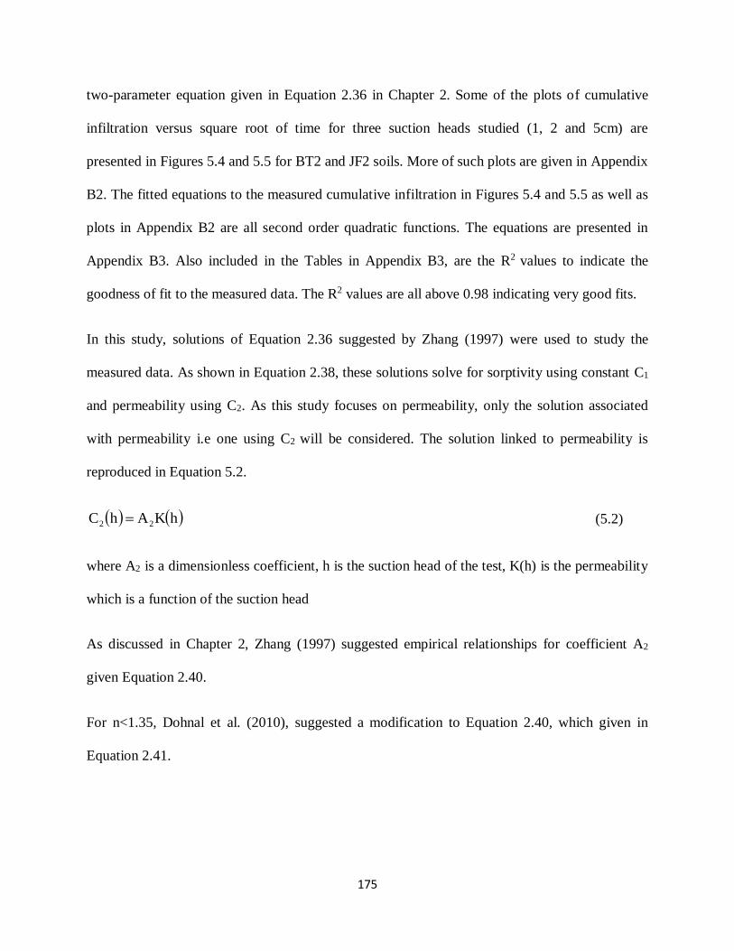
175

two-parameter equation given in Equation 2.36 in Chapter 2. Some of the plots of cumulative

infiltration versus square root of time for three suction heads studied (1, 2 and 5cm) are

presented in Figures 5.4 and 5.5 for BT2 and JF2 soils. More of such plots are given in Appendix

B2. The fitted equations to the measured cumulative infiltration in Figures 5.4 and 5.5 as well as

plots in Appendix B2 are all second order quadratic functions. The equations are presented in

Appendix B3. Also included in the Tables in Appendix B3, are the R2 values to indicate the

goodness of fit to the measured data. The R2 values are all above 0.98 indicating very good fits.

In this study, solutions of Equation 2.36 suggested by Zhang (1997) were used to study the

measured data. As shown in Equation 2.38, these solutions solve for sorptivity using constant C1

and permeability using C2. As this study focuses on permeability, only the solution associated

with permeability i.e one using C2 will be considered. The solution linked to permeability is

reproduced in Equation 5.2.

hKAhC 22 (5.2)

where A2 is a dimensionless coefficient, h is the suction head of the test, K(h) is the permeability

which is a function of the suction head

As discussed in Chapter 2, Zhang (1997) suggested empirical relationships for coefficient A2

given Equation 2.40.

For n<1.35, Dohnal et al. (2010), suggested a modification to Equation 2.40, which given in

Equation 2.41.

176

5.4.1.1 Effect of suction head on infiltration

As discussed earlier, three suction heads: 1, 2 and 5 cm were used in the study. Generally the

infiltration is fastest at 1 cm and slowest at 5 cm irrespective of the compaction effort used as

shown in Figures 5.4 and 5.5 as well as Appendix B2. The rate of infiltration depends on the

difference between the suction at the disk and the suction at the soil surface. At h= -1 cm, the

hydraulic head difference is largest hence the highest infiltration rate.

Because the suction heads are really small and close, the infiltration rates at the three suction

heads can be very close. BT2 soils generally recorded the highest infiltration rates and JF2 the

slowest. Since BT is a granite derivative and JF, generally a clay, this observation is not

surprising.

5.4.1.2 Effect of compaction water content on infiltration

The effect of compaction water content on infiltration can be observed in Figures 5.3 and 5.4 as

well as Appendix B2. In Figures 5.4 and 5.5, the specimens are identified as either being on the

dry of optimum or wet of optimum for BT2 and JF2 soils. It is observed that the infiltration rates

are much higher for specimens on the dry optimum. The dry of optimum specimens have higher

suctions than the wet of optimum specimens as shown in Tables 5.1, 5.2 and 5.3. This implies

that the hydraulic head difference between the dry of optimum specimens and the suction

imposed at the infiltrometer disk is always highest for dry of optimum specimens hence higher

rate of flow into the specimens.

177

(a) Dry of optimum

(b) Wet of optimum

Legend:

Figure 5.4: Cumulative infiltration vs square root time at three suction heads for selected BT2 soil specimens

0

1

2

3

4

5

0 100 200 300 400 500

Cu

mm

ula

tive

infi

ltra

tio

n, (

cm)

Square root of time (√s)

BT2-STD-ASTM13

0

1

2

3

4

5

0 100 200 300 400 500

Cu

mm

ula

tive

infi

ltra

tio

n, (

cm)


BT2-MDF-ASTM8

0

1

2

3

4

5

0 100 200 300 400 500

Cu

mm

ula

tive

infi

ltra

tio

n, (

cm)


BT2-MDF-ASTM11

0

1

2

3

4

5

0 100 200 300 400 500

Cu

mm

ula

tive

infi

ltra

tio

n, (

cm)


BT2-STD-ASTM19.5

0

1

2

3

4

5

0 100 200 300 400 500

Cu

mm

ula

tive

infi

ltra

tio

n, (

cm)


BT2-STD-ASTM22

0

1

2

3

4

5

0 100 200 300 400 500

Cu

mm

ula

tive

infi

ltra

tio

n, (

cm)


BT2-MDF-ASTM16

0

1

2

3

4

5

0100200300400500

Cu

mm

ula

tive

infi

ltra

tio

n, (

cm)


h = -1 cm h = -2 cm h = -5 cm

BT1-MDF-ASTM13

178

(a) Dry of optimum

(b) Wet of optimum

Figure 5.5: Cumulative infiltration vs square root time at three suction heads for selected JF2 soil specimens

0

1

2

3

4

5

0 100 200 300 400 500

Cu

mm

ula

tive

infi

ltra

tio

n, (

cm)


JF2-STD-ASTM10

0

1

2

3

4

5

0 100 200 300 400 500

Cu

mm

ula

tive

infi

ltra

tio

n, (

cm)


JF2-MDF-ASTM8

0

1

2

3

4

5

0 100 200 300 400 500

Cu

mm

ula

tive

infi

ltra

tio

n, (

cm)


JF2-MDF-ASTM11

0

1

2

3

4

5

0 100 200 300 400 500

Cu

mm

ula

tive

infi

ltra

tio

n, (

cm)


JF2-STD-ASTM21

0

1

2

3

4

5

0 100 200 300 400 500

Cu

mm

ula

tive

infi

ltra

tio

n, (

cm)


JF2-STD-ASTM18

0

1

2

3

4

5

0 100 200 300 400 500

Cu

mm

ula

tive

infi

ltra

tio

n, (

cm)


JF2-MDF-ASTM17

179

In addition to suction, two other factors were examined, soil structure and void ratio. As the

compaction water content increases, the soil structure varies from a flocculated system to a

dispersed system. The dispersed soil structure reduces the available void space for water

infiltration leading to long duration of ponding on the soil surface. The flocculated structure

typical of dry of optimum specimens has been described to have a dual porosity structure

(Ahmed et al., 1974; Delage et al., 1996).It would therefore be expected that the macropores

between the clods on the dry of optimum provide preferential paths for infiltration. However,

Clothier and White (1981) note that since disk infiltrometers supply only a small tension at the

soil surface, the effects of macropores on the infiltration are eliminated thus ensuring that

infiltration is only influenced by the properties of the soil matrix. With the elimination of

macroporosity, the remaining influencing factors to infiltration are microstruture and soil

suction. Mitchell (1976) defines microstructure as the elementary particle association within the

soil while macrostructure refers to the arrangement of the soil aggregates.

A further study on the influence of compaction water content is shown in Figures 5.6 and 5.7 and

Appendix B4A in which the infiltration rates are studied for different compaction water contents

at given suction heads for both specimens compacted at both standard and modified Proctor

efforts . Plots for BT1 soil specimens are shown in Figure 5.6 while Figure 5.7 shows plots for

JF2 soil specimens. The plots for BT2 soil specimens are shown in Appendix B4A. It is observed

that for all the three suction heads, infiltration reduces with increase in compaction water content

irrespective of the compaction effort.

180

(a) Standard Proctor

(b) Modified Proctor

Figure 5.6: Comparison of infiltration rates for different compaction water contents at given suction heads for BT1 soils compacted at

standard and modified Proctor efforts

0

1

2

3

4

5

0 100 200 300 400 500

Cu

mm

ula

tive

infi

ltra

tio

n, c

m

Square root of time( √s)

BT1-STD-ASTM10BT1-STD-ASTM13BT1-STD-ASTM16BT1-STD-ASTM18BT1-STD-ASTM20h = -1cm

0

1

2

3

4

5

0 100 200 300 400 500

Cu

mm

ula

tive

infi

ltra

tio

n, c

m



0

1

2

3

4

5

0 100 200 300 400 500

Cu

mm

ula

tive

infi

ltra

tio

n, c

m



0

1

2

3

4

5

0 100 200 300 400 500

Cu

mm

ula

tive

infi

ltra

tio

n, c

m


BT1-MDF-ASTM7

BT1-MDF-ASTM10

BT1-MDF-ASTM13

BT1-MDF-ASTM16

BT1-MDF-ASTM18h = -1cm0

1

2

3

4

5

0 100 200 300 400 500

Cu

mm

ula

tive

infi

ltra

tio

n, c

m


BT1-MDF-ASTM7

BT1-MDF-ASTM10

BT1-MDF-ASTM13

BT1-MDF-ASTM16

BT1-MDF-ASTM18h = -2cm0

1

2

3

4

5

0 100 200 300 400 500

Cu

mm

ula

tive

infi

ltra

tio

n, c

m


BT1-MDF-ASTM7

BT1-MDF-ASTM10

BT1-MDF-ASTM13

BT1-MDF-ASTM16

BT1-MDF-ASTM18h = -5cm

181

(a) Standard Proctor

(b) Modified Proctor

Figure 5.7: Comparison of infiltration rates for different compaction water contents at given suction heads for JF2 soils compacted at

standard and modified Proctor efforts.

0

1

2

3

4

5

0 100 200 300 400 500

Cu

mm

ula

tive

infi

ltra

tio

n, c

m


JF2-STD-ASTM10JF2-STD-ASTM14JF2-STD-ASTM16JF2-STD-ASTM18JF2-STD-ASTM21

h = -1cm0

1

2

3

4

5

0 100 200 300 400 500

Cu

mm

ula

tive

infi

ltra

tio

n, c

m



h = -2cm0

1

2

3

4

5

0 100 200 300 400 500

Cu

mm

ula

tive

infi

ltra

tio

n, c

m



h = -5cm

0

1

2

3

4

5

0 100 200 300 400 500

Cu

mm

ula

tive

infi

ltra

tio

n, c

m


JF2-MDF-ASTM8JF2-MDF-ASTM11JF2-MDF-ASTM13.5JF2-MDF-ASTM15JF2-MDF-ASTM17h = -1cm

0

1

2

3

4

5

0 100 200 300 400 500

Cu

mm

ula

tive

infi

ltra

tio

n, c

m


JF2-MDF-ASTM8JF2-MDF-ASTM11JF2-MDF-ASTM13.5JF2-MDF-ASTM15JF2-MDF-ASTM17h = -2cm

0

1

2

3

4

5

0 100 200 300 400 500

Cu

mm

ula

tive

infi

ltra

tio

n, c

m


JF2-MDF-ASTM8JF2-MDF-ASTM11JF2-MDF-ASTM13.5JF2-MDF-ASTM15JF2-MDF-ASTM17

h = -5cm

182

5.4.1.3 Effect of compaction effort on infiltration

In order to examine the influence of compaction effort on the infiltration, data at the different

suction heads are plotted for specimens compacted at the standard and modified Proctor efforts

as shown in Figure 5.8 and Appendix B4B. Similarly, three factors are at play; the soil suction,

soil structure and void ratio. The influence of compaction effort is not distinct. Figure 5.8 and

plots in Appendix B4B show clusters for specimens compacted dry of optimum and wet of

optimum irrespective of compaction effort. This indicates that suction overrides void ratio in

influencing infiltration into the compacted specimens. The specimens compacted dry of optimum

have higher infiltration rates than those specimens compacted on the wet of optimum.

The influence of void ratio is more glaring by comparing the infiltration of the three soils. The

clayey JF2 soil specimens (CL) have the lowest infiltration rates because of the greater tendency

to pack more densely at the same compaction effort. The coarser BT2 has the highest infiltration

rate.

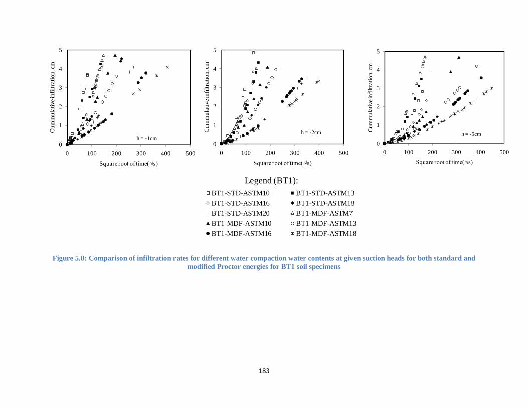
183

Figure 5.8: Comparison of infiltration rates for different water compaction water contents at given suction heads for both standard and

modified Proctor energies for BT1 soil specimens

0

1

2

3

4

5

0 100 200 300 400 500

Cu

mm

ula

tive

infi

ltra

tio

n, c

m


h = -1cm0

1

2

3

4

5

0 100 200 300 400 500

Cu

mm

ula

tive

infi

ltra

tio

n, c

m


h = -2cm

0

1

2

3

4

5

0 100 200 300 400 500

Cu

mm

ula

tive

infi

ltra

tio

n, c

m


h = -5cm

0

1

2

3

4

5

0100200300400500

Cu

mm

ula

tive

infi

ltra

tio

n, c

m


BT1-STD-ASTM10 BT1-STD-ASTM13


BT1-STD-ASTM20 BT1-MDF-ASTM7

BT1-MDF-ASTM10 BT1-MDF-ASTM13


h = -1cm

Legend (BT1):

184

5.4.2 Estimation of near saturated permeability using infiltration measurements

5.4.2.1 Case studies for parameter A2

Parameter A2 in Equation 5.2 can be evaluated using different methods as discussed in Chapter

2, four cases have been evaluated as stated below:

Case 1: The VG SWCC parameters n and α used in the computation of A2 in Equation 2.40 were

obtained by curve fitting the SWCC of the specimen using the VG SWCC equation as shown in

Equation 2.42. For cases where n<1.35, Equation 2.41 suggested by Dohnal et al. (2010) was

used in the computation of A2

Case 2: A2 is evaluated using n and α values suggested by Carsel and Parrish (1988) for different

soil textural classes given in Table 2.4 in Chapter 2.

Case 3: A2 is evaluated with a modification in Carsel and Parrish (1988)’s α parameter. The α

parameter suggested by Carsel and Parrish (1988) was reduced by a factor of 100. The

justification for this reduction is discussed in section 5.4.2.2.

Case 4: If n<1.35 according to Carsel and Parrish (1988), Equation 2.41 as suggested by Dohnal

et al. (2010) was used to evaluate A2. This case is motivated by the fact that Dohnal et al. (2010)

correction was later than Carsel and Parrish (1988).

In order to use Carsel and Parrish (1988) values of n and α, the study materials had to be

classified according to the United States Department of Agriculture (USDA) soil textural

triangle. Soils BT1 and JF2 were classified as clay loam while soil BT2 was classified as loam.

Therefore with this textural classification, it is possible to apply n and α suggested by Carsel and

185

Parrish (1988) in Table 2.4. According to Carsel and Parrish (1988), loam has n>1.35 hence Case

4 is not applicable to soil BT2.

Appendix B5 gives a summary of the A2 values evaluated for the different cases at the different

suction heads.

Table 5.4: Summary of C2 coefficientsfor the different soil specimens at the different suction heads

BT1 soil sets Suction head, cm

-1 -2 -5

C2 (ms-1) C2 (ms-1) C2 (ms-1)

STD-ASTM10 3.E-04 2.E-04 9.E-05

STD-ASTM13 1.E-04 2.E-04 1.E-04

STD-ASTM16 2.E-04 2.E-04 7.E-05

STD-ASTM18 5.E-05 7.E-05 2.E-05

STD-ASTM20 3.E-05 2.E-05 1.E-05

MDF-ASTM7 2.E-04 1.E-04 1.E-04

MDF-ASTM10 7.E-05 8.E-05 4.E-05

MDF-ASTM13 5.E-05 6.E-05 2.E-05

MDF-ASTM16 2.E-05 2.E-05 1.E-05

MDF-ASTM18 7.E-06 1.E-05 1.E-05

BT2 soil sets

Suction head, cm

-1 -2 -5

C2 (ms-1) C2 (ms-1) C2 (ms-1)

STD-ASTM13 5.E-06 3.E-06 1.E-06

STD-ASTM16 3.E-06 3.E-06 2.E-06

STD-ASTM19.5 2.E-06 1.E-06 9.E-07

STD-ASTM22 3.E-07 4.E-07 2.E-07

MDF-ASTM8 4.E-06 4.E-06 4.E-06

MDF-ASTM11 4.E-06 4.E-06 2.E-06

MDF-ASTM13 2.E-06 2.E-06 2.E-06

MDF-ASTM15 9.E-08 1.E-07 1.E-07

MDF-ASTM16 8.E-07 6.E-07 3.E-07

JF2 soil sets

Suction head, cm

-1 -2 -5

C2 (ms-1) C2 (ms-1) C2 (ms-1)

STD-ASTM10 2.E-04 1.E-04 9.E-05

STD-ASTM14 1.E-04 1.E-04 7.E-05

STD-ASTM16 8.E-05 6.E-05 6.E-05

STD-ASTM18 5.E-06 6.E-06 6.E-06

STD-ASTM21 1.E-06 2.E-06 2.E-06

MDF-ASTM8 1.E-04 1.E-04 1.E-04

MDF-ASTM11 1.E-04 1.E-04 7.E-05

MDF-ASTM13.5 3.E-05 2.E-05 2.E-05

MDF-ASTM15 6.E-06 1.E-05 1.E-05

MDF-ASTM17 3.E-06 3.E-06 3.E-06

186

With the A2 values obtained for the different cases, permeability values were computed using the

C2 coefficients at the different suction heads. The C2 values are summarized in the sub-tables

given as Table 5.4. The derived permeabilities for all the study cases are summarized in

Appendix B6.

5.4.2.2Soil water characteristic curves (SWCC)

Soil water characteristic curves as determined in the laboratory were fitted with the VG model in

Equation 2.42 to obtain the parameters n and α used for the computation of A2 in Case 1. Unlike

the usual practice of plotting the volumetric water content data against suction, the volumetric

water contents were plotted against absolute suction heads (m). In order to convert the measured

suctions to corresponding pressure heads, the suctions were divided by the unit weight of water,

9.81kN/m3. The SWCCs for cases 1, 2 and 3 are plotted. Typical plots are shown in Figure 5.9

and the rest are presented in Appendix B7.

The VG parameters for case 1 are also given in Appendix B7 including the sum of squared errors

(SSE). For cases 2 and 3, the VG SWCC equation was fitted to the measured SWCC data using

parameters suggested by Carsel and Parrish (1988) as given in Table 2.4. As mentioned earlier

BT1 and JF2 are classified as clay loam while BT2 is a loam according to the USDA

classification. In order to improve the fit, the α value suggested by Carsel and Parrish (1988) was

divided by 100 hence the study Case 3 as stated above. Observing plots in Figure 5.9 and those

in Appendix B7, case 1 gives the best fit to the measured SWCC data and case 2 gives the

poorest fit. There is an observed improvement in the fit in case 3 implying that the α parameter

suggested by Carsel and Parrish (1988) is generally large for the compacted materials studied.

This is not surprising since Carsel and Parrish (1988) developed their parameters using natural

soils which can be substantially different from the compacted soils.

187

Figure 5.9: Typical SWCC plots for the Cases 1, 2 and 3

0

0.1

0.2

0.3

0.4

0.5

0.1 1 10 100 1000 10000

θw

h, m

BT1-STD-ASTM100

0.1

0.2

0.3

0.4

0.5

0.1 1 10 100 1000 10000

θw

h, m

BT2-STD-ASTM130

0.1

0.2

0.3

0.4

0.5

0.1 1 10 100 1000 10000

θw

h, m

JF2-STD-ASTM10

0

0.1

0.2

0.3

0.4

0.5

0.1 1 10 100 1000 10000

θw

h, m

BT1-STD-ASTM200

0.1

0.2

0.3

0.4

0.5

0.1 1 10 100 1000 10000

θw

h, m

BT2-STD-ASTM22

0

0.1

0.2

0.3

0.4

0.5

0.1 1 10 100 1000 10000

θw

h, m

JF2-STD-ASTM21

0

0.1

0.2

0.3

0.4

0.5

0.1110100100010000

θw

h, m

Case 1

Case 2

Case 3

SWCC measured data

BT1-MDF-ASTM16

188

5.4.2.3 Comparison of permeabilities obtained from the falling head permeability test and

mini-disk infiltrometer

The saturated permeability as measured by the flexible wall permeameter was compared with the

near-saturated permeabilities measured using the mini-disk infiltrometer for Cases 1, 2, 3 and

4.The plots in Figure 5.10 show typical comparisons for selected BT2 and JF2 soil specimens.

Other soil sets are presented in Appendix B8. The saturated permeability obtained from the

falling head permeability test is plotted at suction head h=0 while the other permeabilties are

plotted against the corresponding suction heads imposed on the disk during the test i.e., 1, 2, and

5 cm. Since the suction heads used in the study are small, very close to the saturated state (h=0),

it is expected that the permeability values obtained using the infiltrometer should approximate

the saturated permeability of the soil. To check the comparison, the permeabilities at suction

heads 1, 2 and 5 cm for the different study cases were fitted with a straight line as shown in

Figure 5.10 and Appendix B8. The intercepts of the straight lines on the vertical axis where h = 0

cm were read off as the estimation for saturated permeability for the different cases.

The estimated permeability kest was normalized by the corresponding saturated permeability ksat

of the specimens. The ratio of kest/ ksat is plotted against compaction water contents as shown in

Figures 5.11, 5.12 and 5.13 for BT1, BT2 and JF2 soils, respectively. It is observed that kest for

cases 1 and 3 compare best with the saturated permeability especially for soils compacted dry of

optimum. Case 2 generally performs the worst indicating that the parameters suggested by

Carisel and Parrish (1988) may not be suitable for compacted soils. This is shown by Case 3

where kest substantially improves when the α value suggested by Carsel and Parrish (1988) is

reduced by 100.

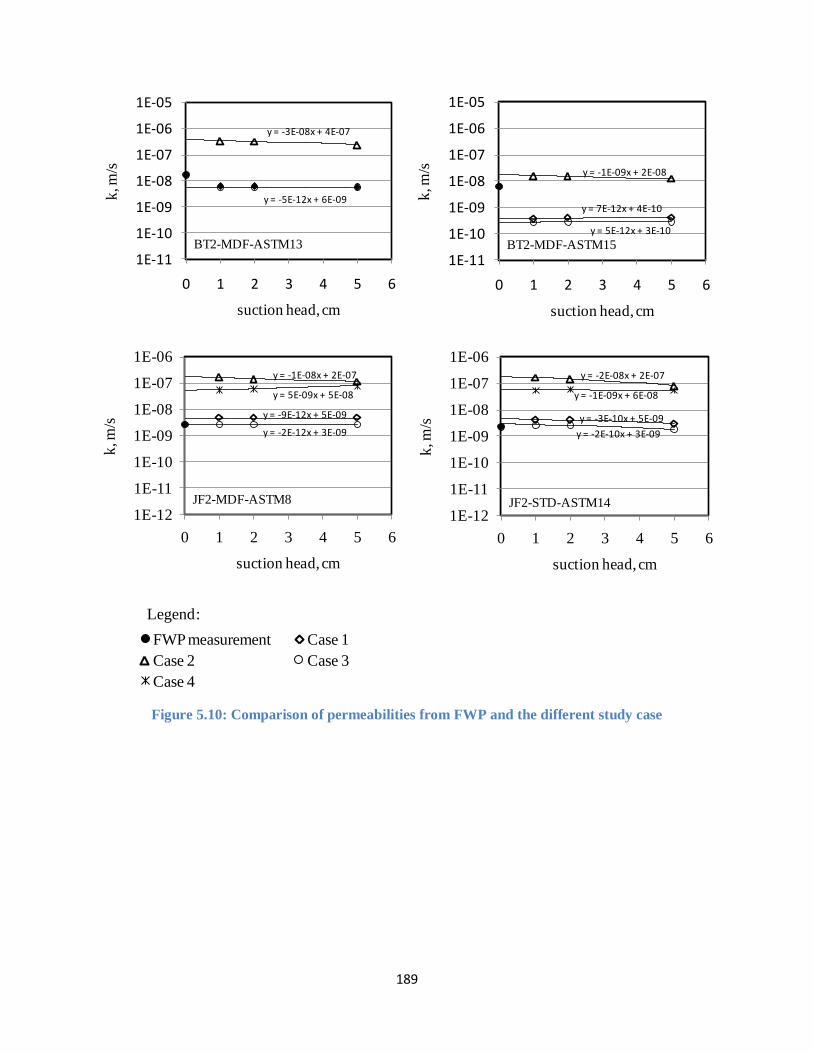
189

Figure 5.10: Comparison of permeabilities from FWP and the different study case

y = -3E-08x + 4E-07

y = -5E-12x + 6E-09

1E-11

1E-10

1E-09

1E-08

1E-07

1E-06

1E-05

0 1 2 3 4 5 6

k, m

/s

suction head, cm

BT2-MDF-ASTM13

y = 7E-12x + 4E-10

y = -1E-09x + 2E-08

y = 5E-12x + 3E-10

1E-11

1E-10

1E-09

1E-08

1E-07

1E-06

1E-05

0 1 2 3 4 5 6

k, m

/s

suction head, cm

BT2-MDF-ASTM15

y = -9E-12x + 5E-09

y = -1E-08x + 2E-07

y = -2E-12x + 3E-09

y = 5E-09x + 5E-08

1E-12

1E-11

1E-10

1E-09

1E-08

1E-07

1E-06

0 1 2 3 4 5 6

k, m

/s

suction head, cm

JF2-MDF-ASTM8

y = -3E-10x + 5E-09

y = -2E-08x + 2E-07

y = -2E-10x + 3E-09

y = -1E-09x + 6E-08

1E-12

1E-11

1E-10

1E-09

1E-08

1E-07

1E-06

0 1 2 3 4 5 6

k, m

/s

suction head, cm

JF2-STD-ASTM14

y = -2E-08x + 1E-07

y = -2E-10x + 2E-09

y = -3E-09x + 5E-08

1E-12

1E-11

1E-10

1E-09

1E-08

1E-07

1E-06

0 1 2 3 4 5 6

k, m

/s

suction head, cm

FWP measurement Case 1

Case 2 Case 3

Case 4

BT1-MDF-ASTM10

Legend:

190

Figure 5.11: Comparison of saturated and estimated permeabilities for different cases for BT1 soil

Figure 5.12: Comparison of saturated and estimated permeabilities for different cases for BT2 soil

0.01

0.10

1.00

10.00

100.00

5 10 15 20 25

kes

t./k

sat


BT1 soil

0.01

0.10

1.00

10.00

100.00

5 10 15 20 25

kes

t./k

sat


case1

case2

case3

case4

JF2 soil

Legend:

0.01

0.10

1.00

10.00

100.00

5 10 15 20 25

kes

t./k

sat


BT2 soil

0.01

0.10

1.00

10.00

100.00

5 10 15 20 25

kes

t./k

sat


case1

case2

case3

case4

JF2 soil

Legend:

191

Figure 5.13: Comparison of saturated and estimated permeabilities for different cases for JF2 soil

Dohnal et al. (2010)’s correction applied in Case 4 improves the estimate of permeability using

Carsel and Parrish (1988) parameters but only dismally. Infact the permeabilities remain at the

same order. The estimates for cases 1 and 3 get worse as compaction water contents increases

implying that the mini-disk infiltrometer is best suited for dry soils with rapid infiltration. In

summary, all the estimates of permeability are within two orders of the saturated permeability

which suggests acceptability of the disk infiltrometer test for estimating near saturated

permeabilities of the compacted soils.

5.5 Statistical permeability model

As stated above, measurements of unsaturated permeability are quite tedious, time consuming,

require expensive equipment and high level of expertise. It was against this background that

indirect methods were formulated. One such method is the statistical model. As noted earlier, the

statistical permeability model is quite rigorous and hence most reliable of all permeability

0.01

0.10

1.00

10.00

100.00

5 10 15 20 25

kes

t./k

sat


JF2 soil

0.01

0.10

1.00

10.00

100.00

5 10 15 20 25

kes

t./k

sat


case1

case2

case3

case4

JF2 soil

Legend:

192

models (Leong and Rahardjo, 1997a). With a saturated permeability value, ks, the permeability

function can be estimated using a statistical model (Fredlund et al., 2012). In this work, since ks

(m/s) values have been determined from the flexible wall permeameter, an attempt was made to

compute the permeability function for the different soil specimens in order to evaluate the

various influences on the permeability function.

Figure 5.14 and 5.15 show the variation of relative permeability kr with suction for the different

soil specimens studied. At a given suction, the wet of optimum specimens have a higher kr value

than the dry of optimum specimens, a reflection of the structural differences as well as pore size

distribution. Given the dispersed structure typical of wet of optimum specimens, desaturation is

much slower and consequently the continuity of the water phase is retained much longer hence a

higher kr value. Also notable is that the permeability functions have a narrower band for

specimens compacted at modified Proctor effort, a reflection of a more uniform pore size

distribution and a more related structure. Mitchell et al. (1966) note that increased compaction

effort leads to a more dispersed structure.

193

Figure 5.14: Variation of kr with suction for soil specimens compacted at standard Proctor effort

1.E-12

1.E-10

1.E-08

1.E-06

1.E-04

1.E-02

1.E+00

0.1 1 10 100 1000 10000 100000 1000000

Rel

ati

ve

Per

mea

bil

ity,

kr

Suction, kPa

BT1-STD-ASTM20

BT1-STD-ASTM18

BT1-STD-ASTM16

BT1-STD-ASTM13

BT1-STD-ASTM10

1.E-12

1.E-10

1.E-08

1.E-06

1.E-04

1.E-02

1.E+00

0.1 1 10 100 1000 10000 100000 1000000

Rel

ati

ve

Per

mea

bil

ity,

kr

Suction, kPa

BT2-STD-ASTM22

BT2-STD-ASTM19.5

BT2-STD-ASTM16

BT2-STD-ASTM13

1.E-12

1.E-10

1.E-08

1.E-06

1.E-04

1.E-02

1.E+00

0.1 1 10 100 1000 10000 100000 1000000

Rel

ati

ve

Per

mea

bil

ity,

kr

Suction, kPa

JF2-STD-ASTM21

JF2-STD-ASTM18

JF2-STD-ASTM16

JF2-STD-ASTM14

JF2-STD-ASTM10

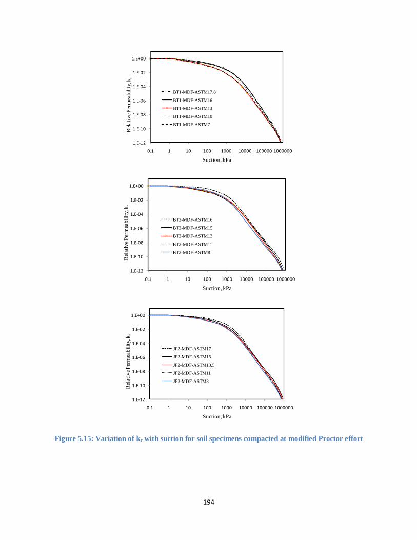
194

Figure 5.15: Variation of kr with suction for soil specimens compacted at modified Proctor effort

1.E-12

1.E-10

1.E-08

1.E-06

1.E-04

1.E-02

1.E+00

0.1 1 10 100 1000 10000 100000 1000000

Rel

ati

ve

Per

mea

bil

ity,

kr

Suction, kPa

BT1-MDF-ASTM17.8

BT1-MDF-ASTM16

BT1-MDF-ASTM13

BT1-MDF-ASTM10

BT1-MDF-ASTM7

1.E-12

1.E-10

1.E-08

1.E-06

1.E-04

1.E-02

1.E+00

0.1 1 10 100 1000 10000 100000 1000000

Rel

ati

ve

Per

mea

bil

ity,

kr

Suction, kPa

BT2-MDF-ASTM16

BT2-MDF-ASTM15

BT2-MDF-ASTM13

BT2-MDF-ASTM11

BT2-MDF-ASTM8

1.E-12

1.E-10

1.E-08

1.E-06

1.E-04

1.E-02

1.E+00

0.1 1 10 100 1000 10000 100000 1000000

Rel

ati

ve

Per

mea

bil

ity,

kr

Suction, kPa

JF2-MDF-ASTM17

JF2-MDF-ASTM15

JF2-MDF-ASTM13.5

JF2-MDF-ASTM11

JF2-MDF-ASTM8

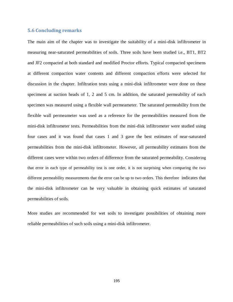
195


The main aim of the chapter was to investigate the suitability of a mini-disk infiltrometer in

measuring near-saturated permeabilities of soils. Three soils have been studied i.e., BT1, BT2

and JF2 compacted at both standard and modified Proctor efforts. Typical compacted specimens

at different compaction water contents and different compaction efforts were selected for

discussion in the chapter. Infiltration tests using a mini-disk infiltrometer were done on these

specimens at suction heads of 1, 2 and 5 cm. In addition, the saturated permeability of each

specimen was measured using a flexible wall permeameter. The saturated permeability from the

flexible wall permeameter was used as a reference for the permeabilities measured from the

mini-disk infiltrometer tests. Permeabilities from the mini-disk infiltrometer were studied using

four cases and it was found that cases 1 and 3 gave the best estimates of near-saturated

permeabilities from the mini-disk infiltrometer. However, all permeability estimates from the

different cases were within two orders of difference from the saturated permeability. Considering

that error in each type of permeability test is one order, it is not surprising when comparing the two

different permeability measurements that the error can be up to two orders. This therefore indicates that

the mini-disk infiltrometer can be very valuable in obtaining quick estimates of saturated

permeabilities of soils.

More studies are recommended for wet soils to investigate possibilities of obtaining more

reliable permeabilities of such soils using a mini-disk infiltrometer.

196

Chapter 6. Unconfined Compressive Strength and Tensile Strength of

compacted soils

6.1 Introduction

Experimental studies (Cuisinier and Laloui, 2004, Koliji et al., 2006, Tarantino, 2011) have

demonstrated that the structure of compacted soils evolves with changing mechanical or

hydraulic regimes that the soils are subjected. It is also well documented that changes in climatic

conditions affect the matric suction of unsaturated soils; decreasing during wetting and

increasing during drying. With changes in both the structure and the matric suction of the soil, it

is expected that strength, compressibility, and hydraulic conductivity of the soil will be affected.

Tensile strength determination is also increasingly becoming useful in studying effects of matric

suction on the effects on the mechanical behavior of unsaturated soils and this can substantially

reduce the testing time typical of suction-controlled tests (Akin and Likos, 2017). Piratheepan et

al. (2012) have suggested a criterion of determining cohesion and internal friction angle for

stabilized materials from unconfined compressive strength (UCS) and Brazilian tensile strength

(BTS). This is useful because the UCS and BTS tests are easy to do, affordable and can be done

in a really short time.

This chapter investigates the influence of matric suction, soil structure, and void ratio on the

UCS and BTS of compacted soils using two test series. The first test series investigates the

strength of the as-compacted soil specimens while the second test series studies the strength

evolution of soil specimens compacted wet of optimum as it dries towards the dry of optimum

water content as stated in Chapter 3. Through an evaluation of the changes in UCS and BTS, the

197

contribution of soil structure and matric suction are qualitatively assessed and discussed. Also,

two tensile strength models are evaluated using the test results.

6.2 Test Series 1 - As-compacted soil specimens

As stated earlier, test series 1 involved testing as-compacted soil specimens. In this subsection,

the test results of these specimens are presented and discussed. Figures 6.1 and 6.2, show test

series 1 specimens on the standard Proctor (sP) and modified Proctor (mP) compaction curves.

Compacting of BT2 soil into the plastic mould was extremely difficult on the dry of optimum.

Very often the specimen got stuck in the mould and split diametrically on opening the split

mould. This may be attributed to the high sand content in the Bukit Timah Granite that generated

tremendous friction between the plastic mould and the soil. Because of this difficulty, it proved

difficult to compact specimens on the dry of optimum of the modified Proctor (mP) compaction

curve as shown in Figure 6.1(b).

Tables 6.1, 6.2, 6.3 and 6.4 show the average water content and dry density of the specimens

tested for test series 1 of each soil.

6.2.1 Stress- strain plots for UCS test

Figure 6.3 shows the stress-strain plots from UCS test for specimens compacted at both standard

and modified Proctor efforts. In Figure 6.3, BT1 and JF2 are presented for illustration. Similar

plots for BT2 and JF1 are presented in Appendix C1.

Irrespective of the compaction effort, the dry of optimum specimens show stiffer response during

shearing. Figure 6.3 and Appendix C1 also show the axial strain at failure increases with

compaction water content hence the specimens compacted on the dry of optimum show more

brittle failure compared to specimens on the wet of optimum which are more ductile.

198

(a) BT1 soil

(b) BT2 soil

Figure 6.1: BT1 Test series 1 specimens

1.4

1.5

1.6

1.7

1.8

1.9

2

5 10 15 20 25 30

Dry

den

sity

, Mg/m

3


Test Series 1

S=60% S=80%

S=100%

S=40%

mP

sP

BT1 soil

1.4

1.5

1.6

1.7

1.8

1.9

2

5 10 15 20 25 30

Dry

den

sity

, Mg/m

3


Test Series 1

S=60% S=80%

S=100%

S=40%

mP

sP

BT2 soil

199

(a) JF1

(b) JF2

Figure 6.2: JF Test series 1specimens

1.4

1.5

1.6

1.7

1.8

1.9

2

5 10 15 20 25 30

Dry

den

sity

, Mg/m

3


Test Series 1

S=60% S=80%

S=100%

mP

sP

JF1 soil

1.4

1.5

1.6

1.7

1.8

1.9

2

5 10 15 20 25 30

Dry

den

sity

, Mg/m

3


Test Series 1

S=60% S=80%

S=100%

mP

sP

JF2 soil

200

Table 6.1: Properties of BT1 test specimens

Notation BT1- Compacted at w% ρd(Mg/m3)

STD-PL10 dry of optimum 10 1.64

STD-PL13 dry of optimum 13 1.66

STD-PL16 optimum 16 1.68

STD-PL18 wet of optimum 18 1.69

STD-PL20 wet of optimum 20 1.66

MDF-PL7 dry of optimum 7 1.80

MDF-PL10 dry of optimum 10 1.83

MDF-PL13 optimum 13 1.83

MDF-PL16 wet of optimum 16 1.81

MDF-PL18 wet of optimum 18 1.77

Table 6.2: Properties of BT2 test specimens

Notation BT2- Compacted at w% ρd(Mg/m3)

STD-PL12 dry of optimum 12.0 1.58


STD-PL19.5 wet optimum 19.5 1.68

STD-PL22 wet of optimum 22.0 1.61

MDF-PL8 dry of optimum 8.0 1.78

MDF-PL15 wet of optimum 15.0 1.84


201

Table 6.3: Properties of JF1 test specimens

Notation JF1- Compacted at w% ρd(Mg/m3)


STD-PL18 optimum 18.0 1.63

STD-PL22 wet optimum 22.0 1.63


MDF-PL15 optimum 15.0 1.78

MDF-PL19.5 wet of optimum 19.5 1.74

Table 6.4: Properties of JF2 test specimens

Notation JF2- Compacted at w% ρd(Mg/m3)



STD-PL16 optimum 16.0 1.76





MDF-PL13.5 optimum 13.5 1.88

MDF-PL15.5 wet of optimum 15.5 1.84


202

(a) BT1

(b) JF2

Figure 6.3: Stress-strain plots from UCS test for BT1 and JF2 soil specimens compacted at both


0

200

400

600

800

1000

0 0.05 0.1 0.15

Ax

ial s

tres

s, k

Pa

Axial strain

BT1-STD-PL10

BT1-STD-PL13

BT1-STD-PL16

BT1-STD-PL18

BT1-STD-PL20

0

200

400

600

800

1000

0 0.05 0.1 0.15

Ax

ial s

tres

s, k

Pa

Axial strain

BT1-MDF-PL7

BT1-MDF-PL10

BT1-MDF-PL13

BT1-MDF-PL16

BT1-MDF-PL18

0

200

400

600

800

1000

0 0.05 0.1 0.15

Ax

ial s

tres

s, k

Pa

Axial strain

JF2-STD-PL10

JF2-STD-PL14

JF2-STD-PL16

JF2-STD-PL18

JF2-STD-PL20

0

200

400

600

800

1000

0 0.05 0.1 0.15

Ax

ial s

tres

s, k

Pa

Axial strain

JF2-MDF-PL8

JF2-MDF-PL11

JF2-MDF-PL13.5

JF2-MDF-PL15

JF2-MDF-PL17

203

(a) BT1

(b) JF2

Figure 6.4: Stress-strain plots from UCS test for both standard and modified Proctor compacted

soils

0

200

400

600

800

1000

0 0.05 0.1 0.15

Ax

ial s

tres

s, k

Pa

Axial strain

BT1-STD-PL10

BT1-STD-PL13

BT1-STD-PL16

BT1-STD-PL18

BT1-STD-PL20

BT1-MDF-PL7

BT1-MDF-PL10

BT1-MDF-PL13

BT1-MDF-PL16

BT1-MDF-PL18

0

200

400

600

800

1000

0 0.05 0.1 0.15

Ax

ial s

tres

s, k

Pa

Axial strain

JF2-STD-PL10

JF2-STD-PL14

JF2-STD-PL16

JF2-STD-PL18

JF2-STD-PL20

JF2-MDF-PL8

JF2-MDF-PL11

JF2-MDF-PL13.5

JF2-MDF-PL15

JF2-MDF-PL17

204

The peak strengths are generally higher on the dry of optimum compared to the wet of optimum

specimens. This is due to structural difference and matric suction between specimens on the dry

of optimum and wet of optimum. This is further discussed in the subsequent subsections. In

Figure 6.4 and Appendix C2, the stress-strain plots for specimens compacted at standard and

modified Proctor efforts for the same soil are combined. From Figure 6.4 and Appendix C2, it is

observed that an increase in compaction effort results in higher peak strengths, stiffer stress-

strain behavior, and more brittle failure depicted by the smaller axial strains at failure. In the

following subsection, a further discussion on peak strengths is presented.

6.2.2 Unconfined compressive strength and Brazilian tensile strength

Figure 6.5 shows the variation of UCS, qu and BTS, σt with compaction water content for the

Test series 1 (as-compacted test specimens). From Figure 6.5, it is observed that generally, both

qu and σt show the same trends as the compaction curves, increasing with water content on the

dry side of optimum to a peak value and then reducing with increasing water content. The peaks

of qu and σt generally occur at the optimum water content except for the qu of modified Proctor

compacted samples. This is observed for both BT1 and JF2 soils where the peak qu occurs at less

than the optimum water content. This suggests that both void ratio and compaction water content

influence qu and σt. It has generally been documented that UCS of unsaturated soils is influenced

by both the void ratio and suction (Marinho and Oliveira; 2012, Kato et al., 2005)

The σt data shows more scatter than the qu data, reflecting greater variability in the smaller size

BTS test specimens. For soils that were dynamically compacted in layers as in this study,

inhomogeneity of the test specimen may influence σt depending on the position of the sample

layer from which the test specimen was prepared, i.e., whether it is top, middle or bottom layer

of the sample. Heibrock et al. (2005) attributes this to structural differences induced by the

205

compaction process along the sample height. However, in this study no distinct trend was

observed among specimens compacted at the same compaction energy as shown in Figures 6.6

suggesting that the compacted sample was relatively homogeneous.

Figure 6.5: UCS and BTS with compaction water content-Test series 1

Figure 6.7 shows variation of matric suction with compaction water content. Matric suction

generally decreases with increase in compaction water content, independent of compaction

effort. A similar trend has been observed by other researchers such as Fleureau et al. (2002),

Leong et al. (2003) and Li et al. (2017). The relationship in Figure 6.7 is bi-linear with the break

0

20

40

60

80

100

0

200

400

600

800

1000

5 10 15 20 25

t , kP

a

qu, k

Pa


sp - UCS

mP - UCS

sP - BTS

mP - BTS

mP - Wopt = 13% sP - Wopt = 16%

BT1 soil

0

20

40

60

80

100

0

200

400

600

800

1000

5 10 15 20 25

t , k

Pa

qu, k

Pa


sP - UCS

mP - UCS

sP - BTS

mP - BTS

mP - Wopt = 13% sP - Wopt = 16%

BT2 soil

0

20

40

60

80

100

0

200

400

600

800

1000

5 10 15 20 25

t , k

Pa

qu, k

Pa


sP - UCS

mP - UCS

sP - BTS

sP - BTS

mP - Wopt = 15% sP - Wopt = 18%

JF1 soil

0

20

40

60

80

100

0

200

400

600

800

1000

5 10 15 20 25

t , k

Pa

qu, k

Pa


sP - UCS

mP - UCS

sP - BTS

mP - BTS

mP - Wopt = 13.5% sP - Wopt = 16%

JF2 soil

206

point occurring around the optimum water content. This observation can be explained by soil

fabric. Compaction on the dry side of optimum largely compresses the inter-aggregate voids.

According to Fleureau et al. (2002) and Li et al. (2017), the intra-aggregate voids that contain the

capillary water that influences matric suction, are hardly compressed by the compaction process

on the dry side of optimum. Therefore, an increase in compaction effort will result in more

compression of the inter-aggregate voids hence yielding a denser material but with negligible

effect on matric suction as observed in Figure 6.7. The increase in density explains why

specimens compacted at modified Proctor effort on the dry of optimum have higher UCS

compared to those compacted at standard Proctor effort despite almost having the same matric

suction.

As the compaction water content increases towards the wet of optimum, the fabric becomes more

dispersed and the compaction effort can substantially compress the inter-aggregate voids hence

affecting the matric suction more. The change in matric suction with respect to moulding water

content on the dry side of optimum is less than on the wet side of optimum. Fleureau et al.

(2002) and Li et al. (2017) have defined the slopes of both lines as suction capacity C given in

Equation 6.1:

(6.1)

where is suction, w is compaction water content and z is a constant. A summary of C and z

together with the coefficient of determination, R2 is shown in Table 6.5.

The low values of R2 for BT2 standard Proctor compacted specimens on the dry of optimum and

BT2 modified Proctor compacted specimens may be attributed to insufficient tests. A better fit is

expected if the number of test increases.

log .C w z

207

Figure 6.6: Variability of the BTS for disk specimens taken from different compaction layers with

dry density-Test series 1

0

20

40

60

80

100

120

1.4 1.5 1.6 1.7 1.8 1.9 2

σt,

kP

a

Dry density, Mg/m3

Top layer - sP

Middle layer - sP

Bottom layer - sP

Top layer - mP

Middle layer - mP

Bottom layer - mP

BT1 soil

0

20

40

60

80

100

120

1.4 1.5 1.6 1.7 1.8 1.9 2

σt,

kP

a

Dry density, Mg/m3

Top layer - sP

Middle layer - sP

Bottom layer - sP

Top layer - mP

Middle layer - mP

Bottom layer - mP

BT2 soil

0

20

40

60

80

100

120

1.4 1.5 1.6 1.7 1.8 1.9 2

σt,

kP

a

Dry density, Mg/m3

Top layer - sP

Middle layer - sP

Bottom layer - sP

Top layer - mP

Middle layer - mP

Bottom layer - mP

JF1 soil

0

20

40

60

80

100

120

1.4 1.5 1.6 1.7 1.8 1.9 2

σt,

kP

a

Dry density, Mg/m3

Top layer - sP

Middle layer - sP

Bottom layer - sP

Top layer - mP

Middle layer - mP

Bottom layer - mP

JF2 soil

208

Figure 6.7: Variation of suction with compaction water content

10

100

1000

10000

5 10 15 20 25

Su

ctio

n, k

Pa


sP

mP

Bestfit - sP

Bestfit -mP

BT1 soil

10

100

1000

10000

5 10 15 20 25

Su

ctio

n, k

Pa


sP

mP

Bestfit - sP

Bestfit -mP

BT2 soil

10

100

1000

10000

5 10 15 20 25

Su

ctio

n, k

Pa


sP

mP

Bestfit - sP

Bestfit - mP

JF1 soil

10

100

1000

10000

5 10 15 20 25

Su

ctio

n, k

Pa


sP

mP

Bestfit - sP

Bestfit - mP

JF2 soil

209

Table 6.5: Relationship of suction with compaction water content

Soil

Standard Proctor

Dry of optimum Wet of optimum

C Z R2 C z R2

BT1 0.077 4.157 0.895 0.145 5.235 0.892

BT2 0.042 3.678 0.677 0.194 5.891 0.889

JF1 0.078 4.371 0.915 0.108 4.921 0.985

JF2 0.065 3.807 0.949 0.240 6.603 0.915

Soil

Modified Proctor

Dry of optimum Wet of optimum

C Z R2 C z R2

BT1 0.067 4.027 0.972 0.123 4.837 0.936

BT2 0.032 3.580 0.447 0.073 4.107 0.593

JF1 0.084 4.425 0.911 0.090 4.590 0.924

JF2 0.077 3.890 0.938 0.141 4.884 0.999

6.3 Test Series 2 -Pre-dried specimens compacted wet of optimum

In order to examine further the influence of matric suction and soil fabric on soil strength, test

series 2 was conducted. Test series 2, comprises sample sets A to I, compacted wet of optimum

using the plastic mould. Each sample set consists of more than 10 specimens. As described in

Chapter 3, the specimens were then dried in airtight desiccators containing saturated NaCl

solutions to selected water contents before testing. On attaining the desired water content, the

UCS, qu and BTS, σt of the specimens were determined.

210

Figures 6.8, 6.9 and 6.10 show the test series 2 specimens on the compaction curves for BT1,

BT2 and JF2 soils, respectively. The soil sets are labelled A-I. The average properties of the soil

sets are given in Table 6.6.

Figure 6.8: BT1 test series 2 specimens

Figure 6.9: BT2 test series 2 specimens

1.4

1.5

1.6

1.7

1.8

1.9

2

5 10 15 20 25 30

Dry

den

sity

, Mg/m

3


S=60% S=80%

S=100%

S=40%

B

C

D

A

Test Series 2mP

sP

BT1 soil

1.4

1.5

1.6

1.7

1.8

1.9

2

5 10 15 20 25 30

Dry

den

sity

, Mg/m

3


S=60% S=80%

S=100%

S=40%

E

F

Test Series 2

mP

sP

BT2 soil

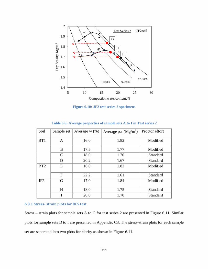
211

Figure 6.10: JF2 test series 2 specimens

Table 6.6: Average properties of sample sets A to I in Test series 2

Soil Sample set Average w (%) Averaged (Mg/m3) Proctor effort

BT1 A 16.0 1.82 Modified

B 17.5 1.77 Modified

C 18.0 1.70 Standard

D 20.2 1.67 Standard

BT2 E 16.0 1.82 Modified

F 22.2 1.61 Standard

JF2 G 17.0 1.84 Modified

H 18.0 1.75 Standard

I 20.0 1.70 Standard

6.3.1 Stress- strain plots for UCS test

Stress – strain plots for sample sets A to C for test series 2 are presented in Figure 6.11. Similar

plots for sample sets D to I are presented in Appendix C3. The stress-strain plots for each sample

set are separated into two plots for clarity as shown in Figure 6.11.

1.4

1.5

1.6

1.7

1.8

1.9

2

5 10 15 20 25 30

Dry

den

sity

, Mg/m

3


S=60% S=80%

S=100%

Test Series 2mP

sP

JF2 soil

G

H

I

212

As the specimens dry, their stiffness and strength increase while their axial strain at failure

reduces i.e. becoming more brittle. A point is reached when the specimens display no more

increase in stiffness and the increase in strength is negligible as shown in the second plot of

stress-strain curves for each of the sample sets in Figure 6.11 and Appendix C3. Because no

substantial increase in stiffness was observed, the stress-strain curves are represented by an

average curve.

Figure 6.12 and Appendix C4 show the UCS, qu and BTS, σt plotted together with the SWCC

and shrinkage curve data of the soil specimens. The shrinkage curve data consists of the volume

measurements of the SWCC, UCS and BTS specimens. It is observed that the shrinkage curve

data from the SWCC specimens which were pre-saturated generally have slightly higher void

ratios at similar water content when compared to the UCS and BTS specimens. This can be

attributed to swelling of the SWCC specimens due to saturation. The SWCC data was fitted with

Fredlund and Xing (1994) SWCC equation using correction factor as unity following

recommendation of Leong and Rahardjo (1997b). The shrinkage curve data was fitted using

Leong and Wijaya (2015)’s universal shrinkage equation.

For all the nine sample sets A to I, drying of the soil specimens from the wet of optimum to dry

of optimum showed an increase in both qu and σt with more remarkable increases noted in qu.

The strength values are observed to increase up to a certain limit and then generally becoming

constant despite further drying or increase in soil suction. Some slight drop in strength at

extremely low water contents were observed especially with σt which can be attributed to

formation of internal micro-fissures common at low water contents in clayey and silty materials

(Sun and Cui, 2017).

213

The degrees of saturation at which qu and σt ceased to increase vary between 82 and 85%, and

between 95 and 97%, respectively, for all the sample sets. Locating these degrees of saturation

on the shrinkage curves indicates that they correspond approximately to the curvature of the

shrinkage curve. As the soils dry, their volume decreases and suction increases. These factors

collectively influence the soil strength. However, the contribution of suction becomes

increasingly minimal past the air-entry value (AEV) of the soil since the water phase becomes

increasingly discontinuous in the soil system. On the other hand, the void ratio may continue to

reduce due to shrinkage contributing to the increase in soil strength. When the shrinkage limit is

reached, the strength ceases to increase and becomes constant. Any variation from the constant

value can be attributed to experimental errors.

214

(a) Sample set A

(b) Sample set B

(c) Sample set C

Figure 6.11: Stress-strain plots for sample sets A, B and C-Test series

0

500

1000

1500

0 0.02 0.04 0.06 0.08 0.1

Ax

ial s

tres

s, k

Pa

Axial strain

16

16

15.8

14

14

13.3

12.3

decreasing water

contentw%

0

500

1000

1500

0 0.02 0.04 0.06 0.08 0.1

Ax

ial s

tres

s, k

Pa

Axial strain

12

11.5

10

9

7.4

6.5

6

5.2

w%

0

500

1000

1500

0 0.02 0.04 0.06 0.08 0.1

Ax

ial s

tres

s, k

Pa

Axial strain

17.7

17.7

17.5

17.5

15.4

14.7

13.1

13

decreasing

water content

w%

0

500

1000

1500

0 0.02 0.04 0.06 0.08 0.1

Ax

ial s

tres

s, k

Pa

Axial strain

12.1

11.2

9

8.5

6.7

6.4

6.1

5.7

w%

0

500

1000

1500

0 0.02 0.04 0.06 0.08 0.1

Ax

ial s

tres

s, k

Pa

Axial strain

18.2

18

18

17

16

15.2

15

14.7

decreasing

water content

w%

0

500

1000

1500

0 0.02 0.04 0.06 0.08 0.1

Ax

ial s

tres

s, k

Pa

Axial strain

12.8

11

10.5

10

9.2

9

7.7

6.2

w%

215

a) Sample set A

(b) Sample set B

(c) Sample set C

Figure 6.12: Variation of UCS and BTS with degree of saturation and SWCC for sample sets A to

C- Test series 2

1

10

100

1000

10000

100000

1000000

0 0.2 0.4 0.6 0.8 1

Matr

ic s

uct

ion o

r st

ren

gth

, kP

a

Degree of Saturation

SWCC

UCS

BTS

S = 80% 95%

0

0.2

0.4

0.6

0.8

1

0 0.1 0.2 0.3

Vo

id r

ati

o

Gravimetric water content

SWCC samples

UCS samples

BTS samples

S = 80% 95%

1

10

100

1000

10000

100000

1000000

0 0.2 0.4 0.6 0.8 1

Matr

ic s

uct

ion o

r st

ren

gth

, kP

a


SWCC

UCS

BTS

S = 80% 95%

0

0.2

0.4

0.6

0.8

1

0 0.1 0.2 0.3

Vo

id r

ati

o


SWCC samples

UCS samples

BTS samples

S = 80% 95%

1

10

100

1000

10000

100000

1000000

0 0.2 0.4 0.6 0.8 1

Matr

ic s

uct

ion o

r st

ren

gth

, kP

a


SWCC

UCS

BTS

S = 80% 95%

0

0.2

0.4

0.6

0.8

1

0 0.1 0.2 0.3

Vo

id r

ati

o


SWCC samples

UCS samples

BTS samples

S = 80% 95%

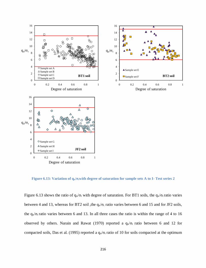
216

Figure 6.13: Variation of qu/σtwith degree of saturation for sample sets A to I- Test series 2

Figure 6.13 shows the ratio of qu/σt with degree of saturation. For BT1 soils, the qu/σt ratio varies

between 4 and 13, whereas for BT2 soil ,the qu/σt ratio varies between 6 and 15 and for JF2 soils,

the qu/σt ratio varies between 6 and 13. In all three cases the ratio is within the range of 4 to 16

observed by others. Narain and Rawat (1970) reported a qu/σt ratio between 6 and 12 for

compacted soils, Das et al. (1995) reported a qu/σt ratio of 10 for soils compacted at the optimum

0

2

4

6

8

10

12

14

16

0 0.2 0.4 0.6 0.8 1

qu/t

Degree of saturation

Sample set A

Sample set B

Sample set C

Sample set DBT1 soil

0

2

4

6

8

10

12

14

16

0 0.2 0.4 0.6 0.8 1

qu/t


Sample set E

Sample set F BT2 soil

0

2

4

6

8

10

12

14

16

0 0.2 0.4 0.6 0.8 1

qu/t


Sample set G

Sample set H

Sample set IJF2 soil

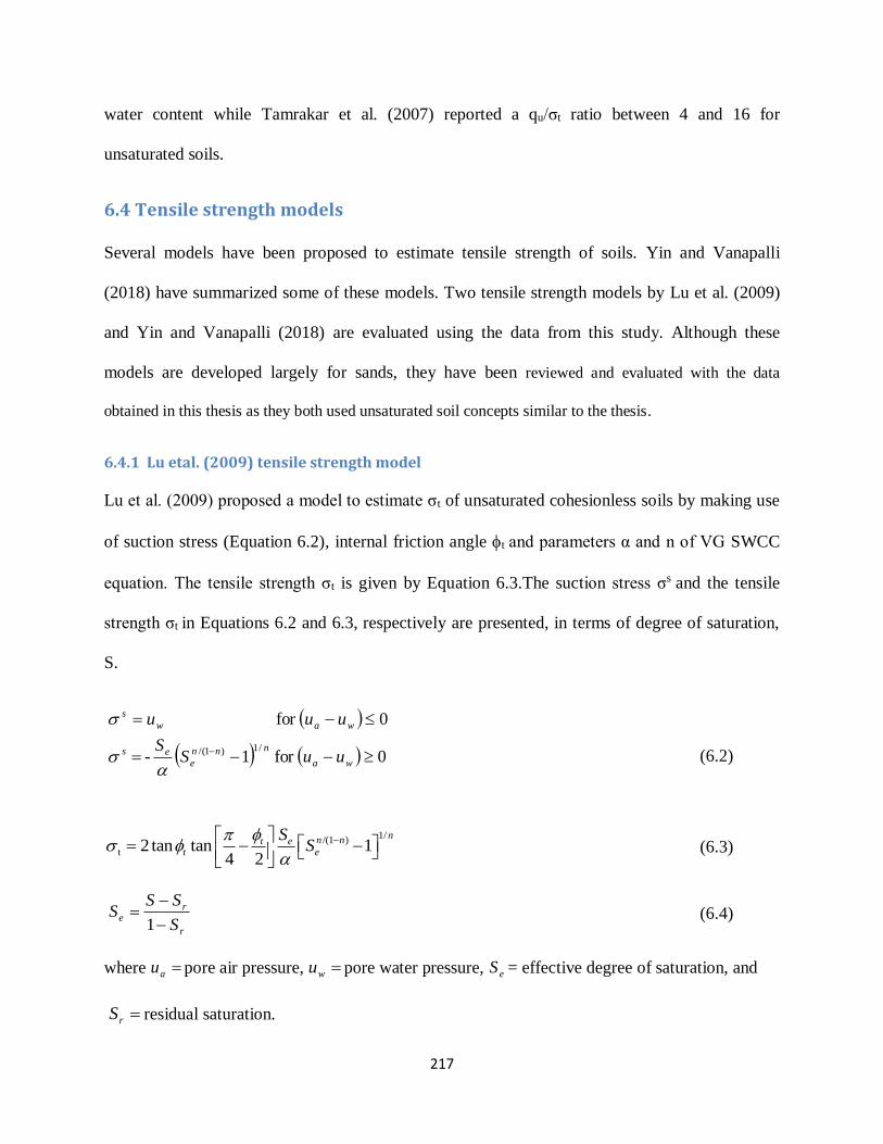
217

water content while Tamrakar et al. (2007) reported a qu/σt ratio between 4 and 16 for

unsaturated soils.

6.4 Tensile strength models

Several models have been proposed to estimate tensile strength of soils. Yin and Vanapalli

(2018) have summarized some of these models. Two tensile strength models by Lu et al. (2009)

and Yin and Vanapalli (2018) are evaluated using the data from this study. Although these

models are developed largely for sands, they have been reviewed and evaluated with the data

obtained in this thesis as they both used unsaturated soil concepts similar to the thesis.

6.4.1 Lu etal. (2009) tensile strength model

Lu et al. (2009) proposed a model to estimate σt of unsaturated cohesionless soils by making use

of suction stress (Equation 6.2), internal friction angle t and parameters α and n of VG SWCC

equation. The tensile strength σt is given by Equation 6.3.The suction stress σs and the tensile

strength σt in Equations 6.2 and 6.3, respectively are presented, in terms of degree of saturation,

S.

(6.2)

(6.3)

(6.4)

where pore air pressure, pore water pressure, = effective degree of saturation, and

residual saturation.

0for 1-

0for

/1)1/(

wa

nnn

ees

waw

s

uuSS

uuu

1//(1 )

t 2 tan tan 14 2

nn nt e

t e

SS

r

re

S

SSS

1

au wu eS

rS

218

Lu et.al (2009) suggest that t can be obtained using a non-linear Mohr-Coulomb envelope in the

low stress zone. Therefore, t was estimated using qu and σt in this study. The slope of the

tangent to the Mohr circles from the UCS and BTS tests as shown in Figure 6.14 was used to

estimatet.

Figure 6.14: Determination of t from UCS and BTS

Plots of these Mohr circles were constructed at different S as the soil dries and hence, a variation

of t with S can be obtained as shown in Figure 6.15 for the soil sets A-I. The t in Figure 6.15 is

denoted as t_exp.

The effective shear strength parameters ’ and c’ from consolidated undrained triaxial tests for

saturated soil specimens of each sample set conducted in accordance to ASTM D4767-11 are

also indicated in Table 6.7.

Based on Figure 6.15, t_exp is not constant but varies with degree of saturation. However, in the

application of Equation 6.3, only a single value of t is admissible. Hence, the sensitivity of is

( – ua)

ua = 0

t 3.1t qu

UCS

BTS

t

'

'

t

219

investigated. A number of cases were evaluated. However, only four significant cases are

presented below:

Case 1: All parameters are as evaluated from experimental data, i.e. and n of the VG equation

from curve fitting the SWCC data while t = '.

Case 2: Values of and n of the VG equation from Case 1 are doubled while t is set to the

lowest value of t_exp and '.

Case 3: Values of and n of the VG equation from Case 1 are doubled while t is set to the

highest value of t_exp and'.

Case 4: Values of and n of the VG equation from Case 1 are doubled while t = '.

To evaluate the performance of Lu et al. (2009) tensile strength model against the experimental

data, the root mean square error (RMSE) is computed. The RMSE is defined in Equation 6.5.

(6.5)

where observed/measured value, model value as predicted at same conditions

as observed value, number of data points

n

XXRMSE

n

i ieliobs

1

2

,mod,

iobsX , ielX ,mod

n

220

Table 6.7: Shear strength and SWCC equations parameters for sample sets A-I

Sampl

e set

From CU tests with

pore-water pressure

measurements φt_exp(o)

Fredlund and Xing

(1994) SWCC

equation’s parameters

van Genuchten

(1980) SWCC

equation’s parameters

φ' (o) c' (kPa) a

(kPa) n m (kPa-1) n

A 26.0 16 16.0 - 40.0 1477 1.577 1.425 0.0010 1.6493

B 27.5 16 15.0 – 40.0 1506 1.278 1.737 0.0011 1.7150

C 27.5 4 28.6 - 45.0 1477 1.247 1.916 0.0013 1.6839

D 27.5 3 15.0 – 40.0 1439 1.541 1.446 0.0010 1.6751

E 30.0 12 45.0-52.0 2000 0.986 2.347 0.0016 1.5727

F 32.0 0 20.0-45.0 4556 0.860 3.329 0.0027 1.4765

G 30.0 10 40.0 – 48.0 1128 1.95 1.256 0.0010 1.9491

H 30.0 5 27.0 – 47.0 1339 1.248 1.839 0.0013 1.6711

I 30.0 10 37.0 – 48.0 1029 1.313 1.593 0.0014 1.7366

221

BT1 soil sets

BT2 soil sets

JF2 soil sets

Figure 6.15: Variation with degree of saturation for sample sets A to G - Test series 2

Figure 6.16 shows the four cases where tensile strength is plotted against degree of saturation for

all the sample sets, A, B, C, D, G,H and I. In Figure 6.16, the SWCC is also plotted. Lu et al.

0

10

20

30

40

50

60

0 0.2 0.4 0.6 0.8 1

t_

exp

o


Set A

Set B

Set C

Set D

0

10

20

30

40

50

60

0 0.2 0.4 0.6 0.8 1

t_

exp

o


Set E

Set F

0

10

20

30

40

50

60

0 0.2 0.4 0.6 0.8 1

t_

exp

o


Set G

Set H

Set I

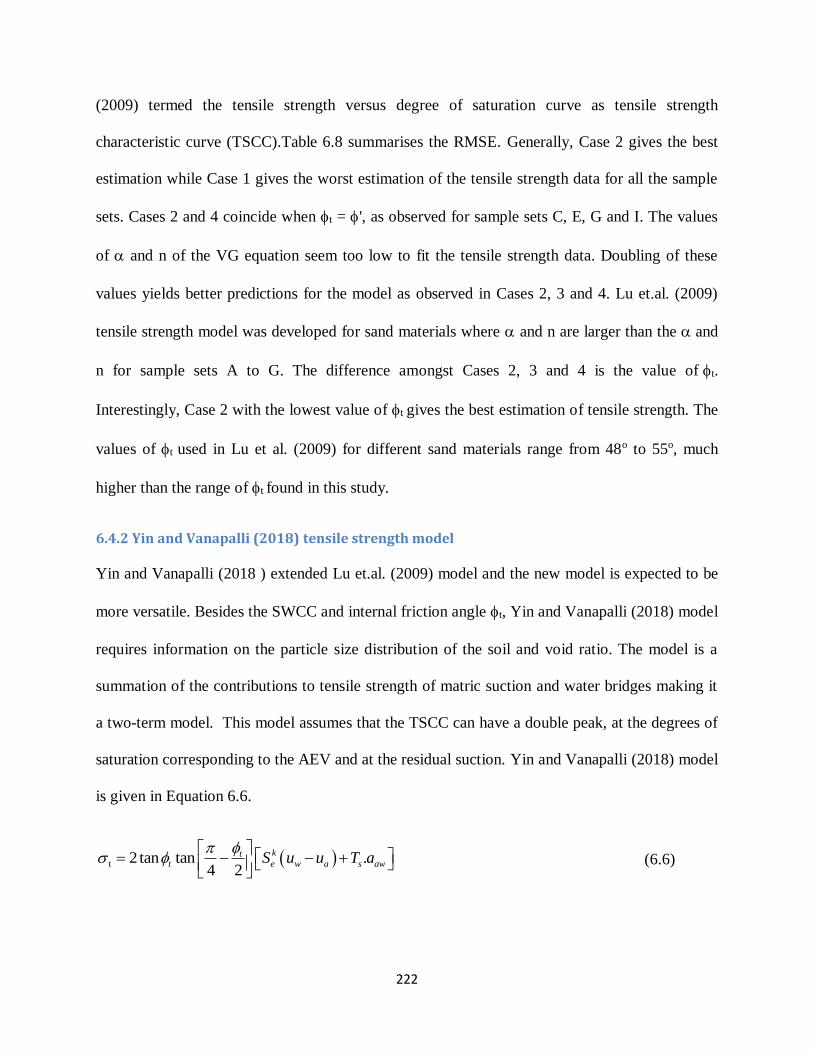
222

(2009) termed the tensile strength versus degree of saturation curve as tensile strength

characteristic curve (TSCC).Table 6.8 summarises the RMSE. Generally, Case 2 gives the best

estimation while Case 1 gives the worst estimation of the tensile strength data for all the sample

sets. Cases 2 and 4 coincide when t = ', as observed for sample sets C, E, G and I. The values

of and n of the VG equation seem too low to fit the tensile strength data. Doubling of these

values yields better predictions for the model as observed in Cases 2, 3 and 4. Lu et.al. (2009)

tensile strength model was developed for sand materials where and n are larger than the and

n for sample sets A to G. The difference amongst Cases 2, 3 and 4 is the value oft.

Interestingly, Case 2 with the lowest value of t gives the best estimation of tensile strength. The

values of t used in Lu et al. (2009) for different sand materials range from 48o to 55o, much

higher than the range of t found in this study.

6.4.2 Yin and Vanapalli (2018) tensile strength model

Yin and Vanapalli (2018 ) extended Lu et.al. (2009) model and the new model is expected to be

more versatile. Besides the SWCC and internal friction angle t, Yin and Vanapalli (2018) model

requires information on the particle size distribution of the soil and void ratio. The model is a

summation of the contributions to tensile strength of matric suction and water bridges making it

a two-term model. This model assumes that the TSCC can have a double peak, at the degrees of

saturation corresponding to the AEV and at the residual suction. Yin and Vanapalli (2018) model

is given in Equation 6.6.

(6.6) t 2 tan tan .

4 2

ktt e w a s awS u u T a

223

where k is a flexibility parameter to give a peak in the TSCC at the AEV, Ts is the surface

tension of water at a given temperature of the fluid in the pores and aaw is the specific air-water

interface area per pore volume.

224

Figure 6.16: Evaluation of Lu et.al (2009) tensile strength model

1

10

100

1000

10000

100000

1000000 Tensile strength

SWCC

Lu et.al (2009) TSCC model- Case 1




Sample Set A

1

10

100

1000

10000

100000

1000000 Sample Set B

1

10

100

1000

10000

100000

1000000 Sample Set C

1

10

100

1000

10000

100000

1000000

Matr

ic s

uct

ion o

r

Ten

sile

str

ength

, kP

a

Sample Set D

1

10

100

1000

10000

100000

1000000 Sample Set G

1

10

100

1000

10000

100000

1000000 Sample Set H

1

10

100

1000

10000

100000

1000000

0 0.2 0.4 0.6 0.8 1


Sample Set I

225

Table 6.8: Summary of RMSE for Lu et.al (2009) tensile strength model

Sample set Case 1 Case 2 Case 3 Case 4

A 721.8 33.7 93.6 54.3

B 382.2 20.6 93.8 57.9

C 576.8 72.9 111.8 72.9

D 835.8 40.6 134.2 95.1

E 1445.0 39.5 70.9 39.5

F 1494.7 8.0 32.4 18.6

G 476.7 92.3 127.8 92.3

H 918.4 64.7 106.3 70.0

I 504.2 60.8 105.0 60.8

Yin and Vanapalli (2018) suggest that aaw is related to void ratio e, mean particle size d50 and two

parameters ɳs and s, as shown in Equation 6.7.

(6.7)

The parameter s, shown in Equation 6.8, is to ensure that the second peak of the TSCC occurs at

the residual degree of saturation, Sr.

(6.8)

eesaw SSed

a s 150

r

rs

S

S

1

226

Therefore with s related to Sr, Yin and Vanapalli (2018) model has two major fitting parameters:

k and s. The parameters k and ɳs are related to the coefficient of uniformity, Cu through

Equations 6.9 and 6.10, respectively.

(6.9a)

where S0= degree of saturation corresponding to first peak of the tensile strength model and Sc =

capillary degree of saturation corresponding to the AEV are related as follows:

(6.9b)

(6.10)

The tensile strength of sample sets A to G do not show any peaks. Similar to the Lu et.al (2009)

tensile strength model, Yin and Vanapalli (2018) model did not fit the experimental data well

and hence, a sensitivity analysis was conducted on the parameters in the model. Although many

cases were evaluated, only four significant cases are presented below:

Case 1: The parameters k and s are computed using Equations 6.9 and 6.10, respectively, while

t= ’.

Case 2: tis equal to the lowest value of t_exp and' while other parameters are same as in

Case1

/ 1

/ 1

1 1 for 6

( 1) 1 0.85 0.15

1 1 for 6

( 1) 1 0.45 0.15

un n

c

un n

c

k Cn S

k Cn S

6for 15.045.0

6for 15.085.0

0

0

u

c

u

c

CS

S

CS

S

us C73.0

227

Case 3: Parameter k is set to 1.5 times the value computed in Case 1, leaving the rest of the

parameters same as Case 1.

Case 4: Parameters k is set to 1.5 times the value in Case 1 while t is equal to the lowest value

of t_exp and ’, leaving all the other parameters same as Case 1.

The void ratio e in Equation 6.7 is taken to be emin from the shrinkage curve (Leong and Wijaya

(2015). For computation of k in Case 1, the ratio S0/Sc was set at 0.9 and 0.6 for BT and JF soils,

respectively, within the range of values given by Equation 6.9b. The shear strength and SWCC

equations parameters are summarized in Table 6.7.

Figure 6.17 shows the four cases where tensile strength is plotted against degree of saturation for

the sample sets A, B, C, D, G,H and I. In Figure 6.17, the SWCC is also plotted. Table 6.9

summarizes the parameters and the RMSE values for all the sample sets. Case 4 gives the lowest

RMSE for all the sample sets as parameter k was best fitted. For all sample sets, Case 1 gives the

worst estimation (highest RMSE) of the tensile strength. Generally, the fit is poorer near

saturation for all the sample sets. Comparing Cases 1 and 2 shows that t affects the tensile

strength slightly with the higher t giving a slightly higher estimate of tensile strength. By

comparing the RMSE values of all the sample sets for Cases 2, 3 and 4, it is observed that the

effect of t is minimal. Therefore, Yin and Vanapalli (2018) tensile strength model largely

depends on the parameters k and s. Comparing the model fits for sample sets A-D (from Bukit

Timah Granite) with sample sets G-I (from Jurong Formation), it is observed that parameter k

has a greater effect on the model fit quality. Despite an increase in s for sample sets G-I, the

quality of fit is poorer largely because of the low values of parameter k. A higher k implies a

reduction in the value of parameter n in the VG equation associated with a soil having a wider

228

pore-size distribution. A large value of s like in the case of sample sets G-I suggests a large

number of interparticle contacts, a complex soil structure and soil fabric both of which are

typical of compacted soils.

Additionally, Yin and Vanapalli (2018) suggest that s represents the anisotropy of the tensile

strength of the material and therefore a large s value points to increased anisotropy in the

distribution of pore water, pore air and consequently the air-water interface as the soil dries up.

Overall, the lowest t give better agreement with the tensile strength data in all cases. Soil sample

sets from the Bukit Timah Granite (A-D) generally show better fit than sample sets from the

Jurong Formation (G-I). This is largely due to the larger k value computed for the sample sets A-

D compared with that computed for sample sets G-I. A larger value of k is associated with coarse

materials expected of A-D sample sets since they are derived from the Bukit Timah Granite. This

is expected since the Yin and Vanapalli (2018) model was developed largely for coarse

materials.

229

Figure 6.17: Evaluation of Yin and Vanapalli (2018) tensile strength model

1

10

100

1000

10000

100000

1000000

1

10

100

1000

10000

100000

1000000

Mat

ric

suct

ion

or

ten

sile

stre

ngt

h, k

Pa

Sample set D

1

10

100

1000

10000

100000

1000000 Tensile strength

SWCC

Yin and Vanapalli (2018) TSCC model- Case 1

Yin and Vanapalli (2018) TSCC model-Case 2

Yin and Vanapalli (2018) TSCC model- Case 3

Yin and Vanapalli (2018)-TSCC model- Case 4

1

10

100

1000

10000

100000

1000000

Sample set A

Sample set B

Sample set C

1

10

100

1000

10000

100000

1000000 Sample set G

1

10

100

1000

10000

100000

1000000 Sample set H

1

10

100

1000

10000

100000

1000000

0 0.2 0.4 0.6 0.8 1Degree of saturation

Sample set I

230

Table 6.9: Parameters for Yin and Vanapalli (2018) tensile strength model for Cases 1 to 4

Sample set

Changed

model

parameters and RMSE

Case 1

t = ’

Case 2

t = min

(’,t_exp)

Case 3

t = ’

(’,t_exp)

Case 4

t = min

(’,t_exp)

Other model

parameters

A ɳs 4.38 4.38 4.38 4.38 e = 0.45

d50 = 0.005 mm Sc= 0.92

Sr = 0.0010

k 4.04 4.04 6.07 6.07

RMSE 114.25 47.09 58.91 39.11

B ɳs 4.38 4.38 4.38 4.38 e = 0.48

d50 = 0.005 mm Sc= 0.90

Sr = 0.0140

k 3.52 3.52 5.29 5.29

RMSE 137.68 52.37 73.94 23.92

C ɳs 4.38 4.38 4.38 4.38 e = 0.515

d50 = 0.005 mm Sc= 0.90

Sr = 0.0010

k 3.61 3.61 5.42 5.42

RMSE 148.63 148.63 92.37 92.37

D ɳs 4.38 4.38 4.38 4.38 e = 0.49 d50 = 0.005 mm

Sc= 0.90

Sr = 0.0010

k 3.64 3.64 5.46 5.46

RMSE 147.74 73.05 94.27 40.10

ɳs 4.38 4.38 4.38 4.38 e = 0.48

E k 4.32 4.32 6.48 6.48 d50=0.02 mm

Sc =0.90

RMSE 44.51 44.51 30.95 30.95 Sr=0.0010

ɳs 4.38 4.38 4.38 4.38

e = 0.57 d50=0.02 mm

F k 2.46 2.46 3.70 3.70 Sc= 0.90

RMSE 117.44 76.26 53.72 28.72 Sr = 0.0010

G ɳs 73 73 73 73 e = 0.44

d50 = 0.02 mm

Sc= 0.92

Sr = 0.0580

k 1.49 1.49 2.24 2.24

RMSE 707.99 707.99 608.17 608.17

H ɳs 73 73 73 73 e = 0.44

d50 = 0.02 mm

Sc= 0.90 Sr = 0.0001

k 1.90 1.90 2.85 2.85

RMSE 811.07 755.51 676.53 629.52

I ɳs 73 73 73 73 e = 0.505

d50 = 0.02 mm

Sc= 0.920 Sr = 0.0065

k 1.77 1.77 2.66 2.66

RMSE 657.04 524.89 552.22 439.15

Hence, the empirical Equations 6.9 and 6.10 suggested by Yin and Vanapalli (2018) are not

applicable for the soils tested in this study.

231

6.4.3 Summary

Two tensile strength models, Lu et al. (2009) and Yin and Vanapalli (2018), were evaluated

against the experimental data in this study. Both models did not perform well using the

parameters as proposed. Both models performed poorer with soil sample sets from the Jurong

Formation (sample sets G-I) compared with those from the Bukit Timah Granite (sample sets A-

D).

Case 2 provides the best estimation of tensile strength for the Lu et al. (2009) model while Case

4 provides the best estimation of tensile strength for the Yin and Vanapalli (2018) model. RMSE

values suggest that Yin and Vanapalli (2018) model performs better than Lu et al. (2009) model

for sample sets A-D while the Lu et.al (2009) model performs better for the sample sets G-I.

However, it should be noted that the Lu et.al (2009) model performs better for JF soil sets (G-I)

because the VG model parameters are doubled (Cases 2 to 4) suggesting more coarseness in the

material compared to the original material (Case 1). This therefore suggests that the Yin and

Vanapalli (2018) generally performs better than the Lu et.al (2009) model. However Lu et.al

(2009) model requires much fewer parameters compared to the Yin and Vanapalli (2018) model,

making it much easier to use.

The models performed better at the lowest t for all degrees of saturation. This is at odd with the

suggestion by Lu et al. (2009) who suggest that t should be higher than ’. However, Lu et al.

(2009)’s tensile strength model was developed from experiments performed on sands. In Yin and

Vanapalli (2018) tensile strength model, the effect of t seems minimal.

Lu et al. (2009)’s tensile strength model is best suited for soils with n in VG equation greater

than 2, i.e. coarse-grained materials, whereas the n obtained for the compacted soils in this study

232

are all less than 2. The empirical relations of k and ɳs suggested by Yin and Vanapalli (2018) are

inadequate for the compacted soils in this study.


This chapter has investigated the unconfined compressive strength and tensile strength of

compacted soils. The effects of soil suction, structure and void ratio on the strength of compacted

soils have been examined. Two tensile strength models were also evaluated using the

experimental data in this study. The main findings are:

There is an interplay of matric suction, soil structure and void ratio influencing soil strength. The

influence of matric suction on strength is minimal for dry soils. The contribution of matric

suction to strength as a near saturated soil dries is significant up to the air-entry value, beyond

which the contribution is negligible as the water phase becomes discontinuous.

The unconfined compressive strength and the Brazilian tensile strength with compaction water

content have the same shape as the compaction curve.

The unconfined compressive strength data shows less scatter than the Brazilian tensile strength

data possibly reflecting the greater variability of smaller specimens in the Brazilian tensile

strength tests.

Although significant increase in the unconfined compressive strength is noted up to the AEV,

strength increase continues up to the shrinkage limit, albeit at a decreased rate. Hence, shrinkage

limit which indicates no further change in void ratio is an important water content in strength of

unsaturated soils.

233

The ratio of unconfined compressive strength to Brazilian tensile strength (qu/σt) lies within the

range of 4 to 15.

The two tensile strength models evaluated were not able to capture the tensile strength of the

compacted soils. Further research is needed to develop better tensile strength models that take

into account the complex structures of compacted soils.

234

Chapter 7. Constant water content shear strength tests on compacted

soils

7.1 Introduction

The common practice of determining shear strength parameters for unsaturated soils is through

consolidated drained (CD) test performed with suction-controlled equipment, either the direct

shear or the triaxial apparatus. These equipment have been reported by several researchers to be

expensive and highly sophisticated hence requiring high level expertise to conduct the tests. In

addition, the test duration is long and the suction range is limited by the HAEV ceramic disk.

The constant water content (CW) test addresses some of these concerns. As mentioned in

Chapter 2, studies have noted that the CW test not only addresses some of the concerns of the

CD test but may actually be more representative of some field stress paths. During a CW test, the

air phase of the soil sample is allowed to drain while the water phase is undrained.

The CW test is usually performed using the axis translation technique (ATT). However recently

some researchers such as de Oliveira et al. (2016) and Marinho et al. (2016) have suggested more

accessible procedures for the CW test that eliminate the need for the ATT. In these procedures,

the CW test is done on the as-compacted soil specimens with matric suctions monitored using a

high capacity tensiometer (HCT) at the base of the specimen. While these tests substantially

reduce testing time and specimens with high matric suctions can be tested, attaining equilibrium

with HCT is sometimes challenging especially with dry soils (high matric suction). The problem

of cavitation was presented in Chapter 2 .

In this study, an attempt is made to evaluate possibility of determining shear strength parameters

of unsaturated soils using compacted soils and conventional soil tests namely, unconfined

235

compression (UC) test, undrained unconsolidated (UU) test and the consolidated undrained

(CU). As discussed in Chapter 3, the UC and UU tests have been done on the as-compacted

(unsaturated) specimens while the consolidated undrained (CU) tests have been done to obtain

saturated shear strength parameters i.e., ϕ’ and c’. Apart from measuring the matric suction of the

as-compacted specimens, no matric suction measurement was done during the test.

The average properties of the test specimens used in this part of the study are the same as those

used for test series 1 in Chapter 6 as given in Figures 6.1 and 6.2 and Tables 6.1 to 6.4.

7.2 Unconfined compression and unconsolidated undrained tests

As mentioned above, UC and UU tests were done on the as-compacted soil specimens. The

observations for these specimens are presented below

7.2.1 Stress-strain behavior

7.2.1.1 Effect of net confining pressure

Figure 7.1 shows typical deviator stress versus axial strain plots of the as-compacted soil

specimens for both the UC and UU tests. The UC tests were done in triplicate. Only selected

plots of soil BT1 are shown in Figure 7.1, the other plots and those of other soil specimens are

presented in Appendix D1. In Figure 7.1, each subplot is for a different compaction water

content as indicated on the plot. For each compaction water content, shearing was done at five

net confining pressures (σ-ua) of 0, 70, 150, 300, 600 kPa. Net confining pressure (σ-ua) = 0

refers to the unconfined compression (UC) test.

At a given compaction water content, an increase in (σ-ua) shows an increase in ductility of the

specimen i.e., the higher the confining pressure, the less distinct is the peak deviator stress. Thu

236

et al. (2006) attributes the increase in ductility to restrained dilation during shearing as a result of

increase in confinement. When dilation is restrained, the peak stress is attained gradually instead

of abruptly.

Figure 7.1 also shows that the axial strain at failure increases as net confining pressure increases.

Specimens at low net confining pressure display behavior similar to overconsolidated clays

which have brittle failure. This is particularly pronounced for specimens compacted dry of

optimum and sheared at low net confining pressure. The stiffness and shear strength increase

with increase in net confining pressure. There is more remarkable increase in shear strength for

specimens compacted dry optimum compared to specimens compacted wet of optimum. On the

wet of optimum, as net confining pressure increases, the specimens tend to get close to saturation

hence increasing net confining pressure may not have great benefit on the shear strength.

237

Legend

Figure 7.1: Deviator stress versus axial strain plots for UC and UU tests

Specimens compacted dry of optimum do not show remarkable change in initial stiffness despite

increase in net confining pressure. The stress-strain curves tend to cluster together showing slight

0

500

1000

1500

2000

0 0.1 0.2 0.3

Dev

iato

r st

ress

, kP

a

Axial strain

BT1-STD-PL10

0

500

1000

1500

2000

0 0.1 0.2 0.3

Dev

iato

r st

ress

, kP

a

Axial strain

BT1-STD-PL18

0

500

1000

1500

2000

0 0.1 0.2 0.3

Dev

iato

r st

ress

, kP

a

Axial strain

BT1-STD-PL13

0

500

1000

1500

2000

0 0.1 0.2 0.3

Dev

iato

r st

ress

, kP

a

Axial strain

BT1-STD-PL20

0

500

1000

1500

2000

0 0.1 0.2 0.3

Dev

iato

r st

ress

, kP

a

Axial strain

BT1-STD-PL16

0

500

1000

1500

2000

0 0.1 0.2 0.3

Dev

iato

r st

ress

, kP

a

Axial strain

600

300

150

70

0

σ3-ua , kPa

238

increment in stiffness despite substantial increase in shear strength. Similar observations are seen

for the other soil specimens presented in Appendix D1.

7.2.1.2 Effect of compaction water content

It has generally been accepted that different compaction water contents yield soils with different

structures hence non-identical soils. Figure 7.2 shows the stress-strain curves for BT1 specimens

compacted at different compaction water contents at various net confining pressure. The other

plots and those of other soil specimens are presented in Appendix D2. Irrespective of compaction

effort at the same confining pressure, the specimens become more brittle as compaction water

content reduces i.e., soil specimens compacted dry of optimum tend to display high brittleness

compared to those soil specimens compacted wet of optimum. The axial strain at failure became

increasingly smaller with reduction in compaction water content. In fact, dry of optimum

specimens in some cases display post-peak softening. This can be attributed to the high suctions

of soil specimens compacted dry of optimum as well as an open structure of these soils. As Thu

et al. (2006) observed, soils with high suctions exhibit overconsolidated behavior hence

increasing the brittle behavior. The open structure plus a high likelihood of internal

microstructures (Sun and Cui, 2017) also contribute to high brittleness. As the specimens get

wetter, their structures become flocculated and they display plastic behavior more typical of

normally consolidated clays.

At a given net confining pressure, peak shear strength increases with reduction in compaction

water content. This is attributed to suction which increases with the compaction water content. It

is interesting to note that for a given compaction effort and net confining pressure, suction seems

to override the void ratio effect i.e., drier specimens display higher shear strength than wetter

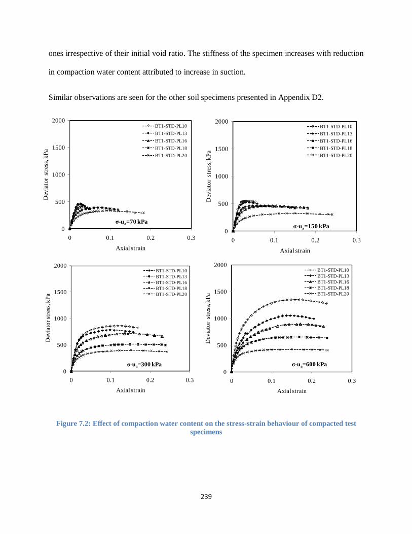
239

ones irrespective of their initial void ratio. The stiffness of the specimen increases with reduction

in compaction water content attributed to increase in suction.

Similar observations are seen for the other soil specimens presented in Appendix D2.

Figure 7.2: Effect of compaction water content on the stress-strain behaviour of compacted test

specimens

0

500

1000

1500

2000

0 0.1 0.2 0.3

Dev

iato

r s

tres

s, k

Pa

Axial strain

BT1-STD-PL10

BT1-STD-PL13

BT1-STD-PL16

BT1-STD-PL18

BT1-STD-PL20

σ-ua=70 kPa

0

500

1000

1500

2000

0 0.1 0.2 0.3

Dev

iato

r s

tres

s, k

Pa

Axial strain

BT1-STD-PL10

BT1-STD-PL13

BT1-STD-PL16

BT1-STD-PL18

BT1-STD-PL20

σ-ua=150 kPa

0

500

1000

1500

2000

0 0.1 0.2 0.3

Dev

iato

r st

ress

, kP

a

Axial strain

BT1-STD-PL10

BT1-STD-PL13

BT1-STD-PL16

BT1-STD-PL18

BT1-STD-PL20

σ-ua=300 kPa

0

500

1000

1500

2000

0 0.1 0.2 0.3

Dev

iato

r s

tres

s, k

Pa

Axial strain

BT1-STD-PL10

BT1-STD-PL13

BT1-STD-PL16

BT1-STD-PL18

BT1-STD-PL20

σ-ua=600 kPa

240

7.2.1.3 Effect of compaction effort

As mentioned earlier, two compaction efforts were used in the study, standard and modified

Proctor. The major influence of increasing compaction effort is the decrease in void ratio.

Typical stress-stain plots are shown in Figure 7.3. The other plots can be found in Appendices

D1 and D2.Figure 7.3 shows that increase in compaction effort generally increases the shear

strength of the soil. At same net confining pressure, specimens compacted at modified Proctor

effort are more brittle that those compacted at standard Proctor effort. Owing to their higher

density (smaller void ratios), specimens compacted at modified Proctor effort show less effect

with net confining pressure and hence are more likely to dilate during shear as compared to the

specimens compacted at standard Proctor effort. Dilation will cause brittle failures and more

post-peak softening. Post-peak softening behavior of dry of optimum specimens compacted at

modified Proctor effort is more persistent than similar specimens compacted at standard Proctor

effort. This can be clearly observed in Appendix D2 at net confining pressure of 600kPa. The

post-peak softening behavior of specimens compacted at standard Proctor effort fades out with

increasing net confining pressure.

Comparing specimens on same side of the optimum, specimens compacted at modified Proctor

effort are generally stiffer than specimens compacted at standard Proctor effort at the same net

confining pressure. This is partly due to smaller void ratios of the modified Proctor compacted

specimens.

241

Figure 7.3: Influence of compaction effort on the stress-strain plots

0

500

1000

1500

2000

0 0.1 0.2 0.3

Ax

ial s

tres

s, k

Pa

Axial strain

σ-ua=300 kPa

0

500

1000

1500

2000

-0.1 0.1 0.3

Ax

ial s

tres

s, k

Pa

Axial strain

BT1-STD-PL10BT1-STD-PL13BT1-STD-PL16BT1-STD-PL18BT1-STD-PL20BT1-MDF-PL7BT1-MDF-PL10BT1-MDF-PL13BT1-MDF-PL16BT1-MDF-PL18

Legend:

0

500

1000

1500

2000

0 0.1 0.2 0.3

Ax

ial s

tres

s, k

Pa

Axial strain

σ-ua=600 kPa

242

7.2.2 Peak strength

As discussed above, the peak strength is influenced by compaction water content, net confining

pressure as well as the compaction effort. Figure 7.4 shows typical plots of variation of peak

unconfined compressive strength (qu) with compaction water content, net confining pressure as

well as compaction effort. The other plots are shown in Appendix D3. It is observed that at a

given compaction water content, peak strength generally increases with increase in confining

pressure. The increase is more pronounced with drier soils. As the compaction water content

increases, there is increasingly less benefit because the soils are tending towards saturation hence

a drop in suction. It is also interesting to note that the variation of unconfined compressive

strength with compaction water content follows almost the same trend as the respective

compaction curves at low net confining pressures. At high net confining pressures, the

unconfined compressive strength decreases as compaction water content increases.

Figure 7.5 shows typical Mohr circles derived from the peak deviator stresses at the different net

confining pressures. Peak deviator stresses for the UC and UU tests together with the failure

axial strains are presented in Appendix D5. The plots in Figure 7.5 show behavior of the

specimens compacted dry and wet of optimum. The specimens compacted dry of optimum show

increase in strength with increasing confining pressure for the range of pressures studied.

Therefore, undrained shear strength of unsaturated soils is a function of the confining pressure.

The specimens on wet of optimum soon get to saturated state as confining pressure is increased.

This is reflected by the Mohr circles negligibly increasing in size as confining pressure increases,

a behavior typical of the φu= 0 concept observed in saturated soils. Under the φu= 0, a horizontal

line can be drawn tangential to all the Mohr circles since any increment in confining pressure is

243

counteracted by an increase in pore water pressure hence resulting in no net increase in the shear

strength. In addition to Figure 7.5, more plots are presented in Appendix D6.

(a) BT1 soil

(b) JF2 soil

Figure 7.4:Peak strength variation with net confining pressure , compaction water content and

compaction efforts

0

500

1000

1500

2000

5 10 15 20 25

qu, k

Pa


0 (UCS)

70

150

300

600

σ3-ua (kPa)

BT1-Standard Proctor energy0

500

1000

1500

2000

5 10 15 20 25q

u, k

Pa


0 (UCS)

70

150

300

600

σ3-ua (kPa)

BT1-modified Proctor energy

0

500

1000

1500

2000

5 10 15 20 25

qu, k

Pa


0 (UCS)

70

150

300

600

σ3-ua (kPa)

JF2-Standard Proctor energy0

500

1000

1500

2000

5 10 15 20 25

qu, k

Pa


0 (UCS)

70

150

300

600

σ3-ua (kPa)

JF2-modified Proctor energy

244

Dry of optimum specimens Wet of optimum specimens

Figure 7.5: Typical Mohr circle plots for the UC and UU tests

-1000

0

1000

2000

-1000 0 1000 2000 3000

τ(k

Pa)

σ-ua(kPa)

BT1-STD-PL10

-1000

0

1000

2000

-1000 0 1000 2000 3000

τ(k

Pa)

σ-ua(kPa)

BT1-STD-PL20

-1000

0

1000

2000

-1000 0 1000 2000 3000

τ(k

Pa)

σ-ua(kPa)

JF2-STD-PL10

-1000

0

1000

2000

-1000 0 1000 2000 3000

τ(k

Pa)

σ-ua(kPa)

JF2-STD-PL20

-1000

0

1000

2000

-1000 0 1000 2000 3000

τ(k

Pa)

σ-ua(kPa)

BT1-MDF-PL7

-1000

0

1000

2000

-1000 0 1000 2000 3000

τ(k

Pa)

σ-ua(kPa)

BT1-MDF-PL18

245

7.3 Saturated shear strength parameters

As mentioned earlier, in order to interpret shear strength behavior of unsaturated soils, it is

important to evaluate the saturated shear strength parameters of the soil i.e., ϕ’ and c’.

Unsaturated shear strength is a combination of the saturated shear strength and contribution to

shear strength from matric suction. Following the idea that compaction water content affects the

structure of the compacted soil, it was assumed that each compaction water content yielded a

different soil and hence for each compaction water content, ϕ’ and c’ were determined using a

CU test described in Chapter 3.Figure 7.6 shows such typical plots of deviator stress versus axial

strain for the multi-stage testing including the derived Mohr-Coulomb envelopes. Appendix D4

shows a summary of CU test data including ϕ’ and c’ for all the compacted specimens.

Figure 7.6: Typical stress-strain plots for the CU multi-stage test and the derived Mohr-Coulomb

envelope

0

200

400

600

800

1000

0 0.05 0.1 0.15 0.2 0.25

Dev

iato

r st

ress

, kP

a

Axial strain

BT1-STD-PL18

0

200

400

0 200 400 600 800

Sh

ear

stre

ngth

(k

Pa)

Effective Normal stress (kPa)

c'=4kPa

ϕ'= 27.5oBT1-STD-PL18

0

200

400

600

800

1000

0 0.05 0.1 0.15 0.2 0.25

Dev

iato

r st

ress

, kP

a

Axial strain

JF2-MDF-PL11

0

200

400

0 200 400 600 800

Sh

ear

stre

ngth

(k

Pa)


ϕ'= 30o

c'=8 kPa

JF2-MDF-PL11

246

Figure 7.7 shows the variation of ϕ’ with compaction water content and compaction dry density,

while similar plots for c’ are shown in Figure 7.8

Figure 7.7:Variation of friction angle with dry density and compaction water content

20

30

40

1.5 1.6 1.7 1.8 1.9

Fri

ctio

n a

ngle

, φ'

Dry density, Mg/m3

BT1 soil sets

20

30

40

5 10 15 20 25

Fri

ctio

n a

ngle

, φ'


BT1 soil sets

20

30

40

1.5 1.6 1.7 1.8 1.9

Fri

ctio

n a

ngle

, φ'

Dry density, Mg/m3

BT2 soil sets

20

30

40

5 10 15 20 25

Fri

ctio

n a

ngle

, φ'


BT2 soil sets

20

30

40

1.5 1.6 1.7 1.8 1.9

Fri

ctio

n a

ngle

, φ'

Dry density, Mg/m3

JF1 soil sets

20

30

40

5 10 15 20 25

Fri

ctio

n a

ngle

, φ'


JF1 soil sets

20

30

40

1.5 1.6 1.7 1.8 1.9

Fri

ctio

n a

ngle

, φ'

Dry density, Mg/m3

JF2 soil sets

20

30

40

5 10 15 20 25

Fri

ctio

n a

ngle

, φ'


JF2 soil sets

20

30

40

1.51.61.71.81.9

Fri

ctio

n a

ngle

, φ'

Dry density, Mg/m3

Standard Proctor specimens modified Proctor specimensLegend:

BT1 soil sets

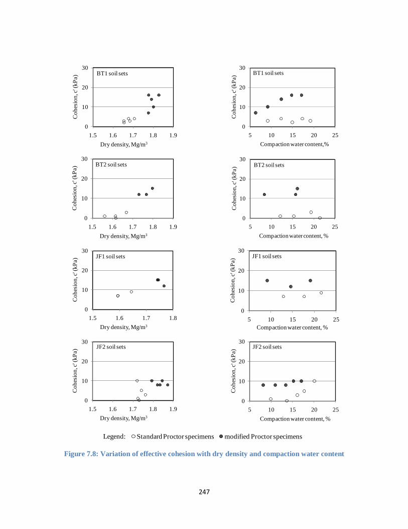
247

Figure 7.8: Variation of effective cohesion with dry density and compaction water content

0

10

20

30

1.5 1.6 1.7 1.8 1.9

Co

hes

ion

, c' (

kP

a)

Dry density, Mg/m3

BT1 soil sets

0

10

20

30

5 10 15 20 25

Co

hes

ion

, c' (

kP

a)


BT1 soil sets

0

10

20

30

1.5 1.6 1.7 1.8 1.9

Co

hes

ion

, c' (

kP

a)

Dry density, Mg/m3

BT2 soil sets

0

10

20

30

5 10 15 20 25

Co

hes

ion

, c' (

kP

a)


BT2 soil sets

0

10

20

30

1.5 1.6 1.7 1.8

Co

hes

ion

, c' (

kP

a)

Dry density, Mg/m3

JF1 soil sets

0

10

20

30

5 10 15 20 25

Co

hes

ion

, c' (

kP

a)


JF1 soil sets

0

10

20

30

1.5 1.6 1.7 1.8 1.9

Co

hes

ion

, c' (

kP

a)

Dry density, Mg/m3

JF2 soil sets

0

10

20

30

5 10 15 20 25

Co

hes

ion

, c' (

kP

a)


JF2 soil sets

20

30

40

1.51.61.71.81.9

Fri

ctio

n a

ngle

, φ'

Dry density, Mg/m3


BT1 soil sets

248

From Figure 7.7 the dependency of ϕ’ on dry density is not obvious. Intuitively, it is expected

that ϕ’ increases with dry density. Although soil structure may also affect ϕ’ coupled with

experimental errors, the variation of ϕ’ over the range of dry density studied is small. A similar

observation has been reported by Marinho et al. (2016). Also as mentioned in section 7.2.1.1,

compacted soils tend to display over-consolidated (OC) behavior at low net confining pressure

and normally consolidated (NC) behavior at high net confining pressure. This has great

implication on the selection of effective confining pressures for the CU test yet very often the

initial stress state of the specimens at the end of the compaction process is unknown. In this

study, effective confining pressures of 80, 150 and 300 kPa were selected taking into account the

limitations of the pressure equipment in the laboratory. Figure 7.9 illustrates the OC and NC

behaviour largely observed with samples compacted dry of optimum. From Figure 7.9a it is

observed that the soil specimen displays OC behavior for the first two Mohr circles and NC

behavior for last Mohr-circle. These effects show the ambiguity in determining saturated shear

strength behavior of compacted soils. In this study, this ambiguity was not explored in further

details. In this study, given the small variation of ϕ’ for the same soil compacted at different

compaction water contents, an average ϕ’ was adopted for each compaction effort for

interpretation of c’. Figure 7.10 shows that when an average effective friction angle is used to

interpret the results, more scatter is observed in the effective cohesion showing a conclusion that

there is a greater uncertainty in the determination of c’, a well known fact in geotechnical

engineering. Table 7.1 presents the minimum, average and maximum ϕ’ for each soil at the

different compaction efforts. Also shown in Table 7.1 is the average ϕ’ for the same soil

regardless of compaction effort. Figure 7.10 shows the interpretation effective cohesion , c’ using

the average friction angle for each compaction effort. If the spread of the friction angles is

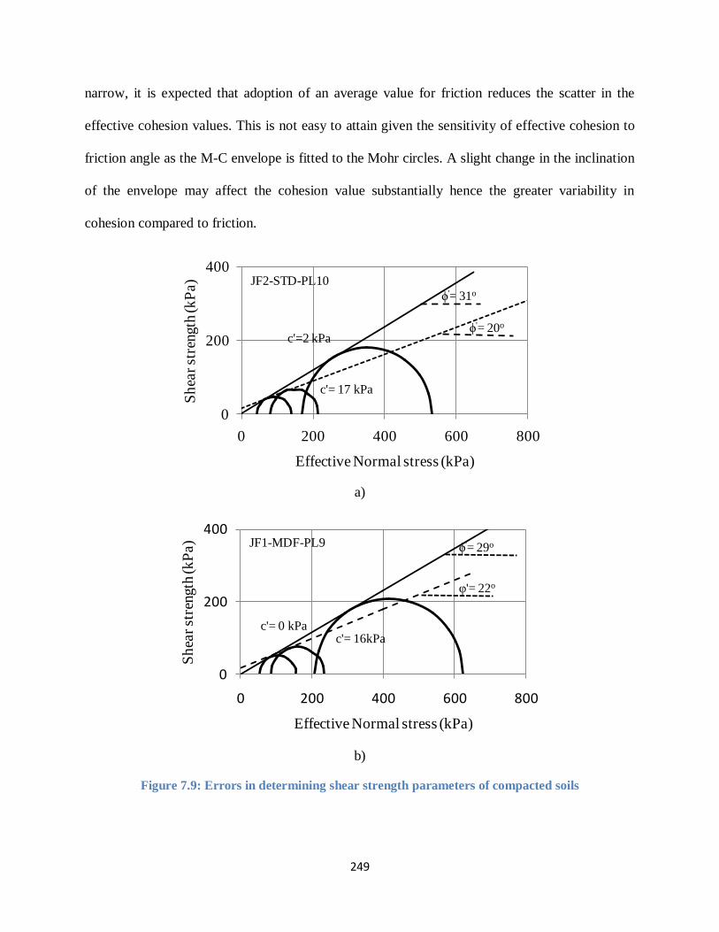
249

narrow, it is expected that adoption of an average value for friction reduces the scatter in the

effective cohesion values. This is not easy to attain given the sensitivity of effective cohesion to

friction angle as the M-C envelope is fitted to the Mohr circles. A slight change in the inclination

of the envelope may affect the cohesion value substantially hence the greater variability in

cohesion compared to friction.

a)

b)

Figure 7.9: Errors in determining shear strength parameters of compacted soils

JF2-STD-PL10

c'= 17 kPa

ϕ'= 31o

0

200

400

0 200 400 600 800

Sh

ear

stre

ngth

(k

Pa)


c'=2 kPaϕ'= 20o

ϕ'= 29o

0

200

400

0 200 400 600 800

Sh

ear

stre

ngth

(k

Pa)


JF1-MDF-PL9

c'= 0 kPac'= 16kPa

φ'= 22o

250

Table 7.1: Variation of friction angles for the different soils

Soil Compaction

Proctor effort

Minimum

φ’(o) Average φ’(o)

Maximum

φ’(o)

Overall

average φ’(o)

BT1 Standard 27.5 28.5 30.6

27.9

Modified 26.0 27.3 29.0

BT2 Standard 29.5 31.1 32.0

30.6

Modified 29.5 29.8 30.0

JF1 Standard 26.5 26.8 27.5

27.0

Modified 25.5 27.2 28.0

JF2

Standard 30.0 30.5 31.0

29.9

Modified 28.0 29.4 30.0

251

Figure 7.10: Effective cohesion using an average friction angle for each compaction effort

0

10

20

30

1.5 1.6 1.7 1.8 1.9

Co

hes

ion

, c' (

kP

a)

Dry density, Mg/m3

BT1 soil sets

0

10

20

30

5 10 15 20 25

Co

hes

ion

, c' (

kP

a)


BT1 soil sets

0

10

20

30

1.5 1.6 1.7 1.8 1.9

Co

hes

ion

, c' (

kP

a)

Dry density, Mg/m3

BT2 soil sets

0

10

20

30

5 10 15 20 25

Co

hes

ion

, c' (

kP

a)


BT2 soil sets

0

10

20

30

1.5 1.6 1.7 1.8

Co

hes

ion

, c' (

kP

a)

Dry density, Mg/m3

JF1 soil sets

0

10

20

30

5 10 15 20 25

Co

hes

ion

, c' (

kP

a)


JF1 soil sets

0

10

20

30

1.5 1.6 1.7 1.8 1.9

Co

hes

ion

, c' (

kP

a)

Dry density, Mg/m3

JF2 soil sets

0

10

20

30

5 10 15 20 25

Co

hes

ion

, c' (

kP

a)


JF2 soil sets

20

30

40

1.51.61.71.81.9

Fri

ctio

n a

ngle

, φ'

Dry density, Mg/m3


BT1 soil sets

252

7.4 Proposed interpretation of the CW test

As discussed above, using peak deviator stresses in Appendix D5, Mohr circles were constructed

as illustrated in Figure 7.5. An attempt is made to derive total cohesion from UC and UU tests

conducted on the as-compacted soil specimens. Lines with slope of ϕ’ are drawn tangentially to

each Mohr circle as shown in Figure 7.11 for selected soil specimens. The rest of the plots are

presented in Appendix D6. It is assumed that as the unsaturated soil specimen is compressed

under the net confining pressure, its degree of saturation will increase resulting in a reduction of

its matric suction. The reduction in matric suction will be reflected in the total cohesion, C given

by the y-intercept of the line shown in Figure 7.11. The total cohesion, C is the sum of the

effective cohesion, c’ (from saturated tests, CU) and the shear strength contribution from matric

suction at zero net normal stress.

Figure 7.12 shows the variation of total cohesion with net normal stress for BT1 soil specimens.

It is observed that the total cohesion remains constant at low net normal stress and then decreases

with increase in net normal stress. This indicates that the matric suction may remain the same as

the as-compacted specimen at low net normal stress and decreases as net normal stress increases.

253

(a) BT1

(b) BT2

(c) JF2

Figure 7.11: Typical plots showing UU Mohr circles fitted with tangent lines at the respective

effective friction angles

-1000

0

1000

2000

-1000 0 1000 2000 3000

τ(k

Pa)

σ(kPa)

BT1-STD-PL10

-1000

0

1000

2000

-1000 0 1000 2000 3000

τ(k

Pa)

σ(kPa)

BT1-STD-PL20

-1000

0

1000

2000

-1000 0 1000 2000 3000

τ(k

Pa)

σ(kPa)

BT2-MDF-PL8

-1000

0

1000

2000

-1000 0 1000 2000 3000

τ(k

Pa)

σ(kPa)

BT2-STD-PL22

-1000

0

1000

2000

-1000 0 1000 2000 3000

τ(k

Pa)

σ(kPa)

JF2-STD-PL10

-1000

0

1000

2000

-1000 0 1000 2000 3000

τ(k

Pa)

σ(kPa)

JF2-STD-PL20

254

Figure 7.12: Variation of total cohesion with net confining pressure for BT1 soils compacted at


Figure 7.13 shows the Mohr circles of specimens compacted dry of optimum. A single tangent

line is able to be drawn to all the Mohr circles revealing that specimens compacted dry of

optimum did not experience a reduction in matric suction when net normal stress increases. This

suggests that it may also be possible to obtain ϕ’ for the specimen without conducting a CU test.

Perhaps this is a similar observation that Marinho et al. (2016) made and concluded that with a

well performed CW test, the CU test may not be necessary. This is an interesting observation

especially for dry soils since they difficult to test using available methods whether ATT or HCT.

This observation is useful in interpreting CW tests. Validating it with more experimental data

would be very gainful in the practice of unsaturated soil mechanics. Assuming this holds largely

true for most soils including the materials studied in this thesis then the as-compacted suction

would be sufficient in fully interpreting a UCS test.

-200

-100

0

100

200

300

0 200 400 600 800

To

tal

coh

esio

n, k

Pa

σ3-ua , kPa

BT1-STD-PL10

BT1-STD-PL13

BT1-STD-PL16

BT1-STD-PL18

BT1-STD-PL20

-200

-100

0

100

200

300

0 200 400 600 800

To

tal

coh

esio

n, k

Pa

σ3-ua , kPa

BT1-MDF-PL7BT1-MDF-PL10BT1-MDF-PL13BT1-MDF-PL16BT1-MDF-PL18

255

Vanapalli (1994) notes that the unconfined compression (UC) test on a dry soil can be assumed

to be conducted at constant suction. In this thesis, only the as-compacted suctions for the soil

specimens were determined using the filter paper method as discussed in Chapter 4. Therefore

with suction measurements, (ua-uw) is available and tanϕb which represents the rate of shear

strength increase with (ua-uw) can be obtained from the total cohesion C given in Equation 2.52.

From Equation 2.52, tanφb is evaluated as given in Equation 7.1

tanb= (C-c’)/(ua-uw) (7.1)

c’ is the effective cohesion obtained from the CU test.

Using the UC test and UU test at the lowest net confining pressure ,tanϕb can be computed from

C using with (ua-uw) and c’ for all the as-compacted specimens. Plots of tanb/tan’ versus

degree of saturation are given in Figure 7.14.

256

The close band of tangents Equivalent tangent line

Figure 7.13: A single line for Mohr circles of specimens compacted dry of optimum

-1000

0

1000

2000

-1000 0 1000 2000 3000

τ(k

Pa)

σ(kPa)

BT1-MDF-PL7

-1000

0

1000

2000

-1000 0 1000 2000 3000

τ(k

Pa)

σ(kPa)

ϕ'= 29oCT= 195 kPa

BT1-MDF-PL7

-1000

0

1000

2000

-1000 0 1000 2000 3000

τ(k

Pa)

σ(kPa)

BT1-STD-PL10

-1000

0

1000

2000

-1000 0 1000 2000 3000

τ(k

Pa)

σ(kPa)

ϕ'= 28.5o

CT= 80 kPa

BT1-STD-PL10

-1000

0

1000

2000

-1000 0 1000 2000 3000

τ(k

Pa)

σ(kPa)

JF2-STD-PL10

-1000

0

1000

2000

-1000 0 1000 2000 3000

τ(k

Pa)

σ(kPa)

JF2-STD-PL10

ϕ'=30o

257

(a) BT1 (b) BT2

(c) JF1 (d) JF2

Figure 7.14: Plots of tanφb/tanφ’ versus degree of saturation for the as-compacted soil specimens

In Figure 7.14, tan b/tan ’ ratios derived from fitting tangents to both the UC and UU at lowest

net confining pressure of 70kPa (UU70) Mohr circles. The assumption for UU70 may not be

correct for the wet of optimum specimens as can be seen for JF2 soil (Figure 7.14d).

0

0.2

0.4

0.6

0.8

1

0 0.2 0.4 0.6 0.8 1

tan

ϕb/t

anϕ

'


From UCS Mohr-circle

From the UU70 Mohr-circle

From UCS M-C (average friction)

From UU70 M-C (average friction)

Line 1:1

BT1 soil sets

0

0.2

0.4

0.6

0.8

1

0 0.2 0.4 0.6 0.8 1

tan

ϕb/t

anϕ

'


Computed using UCS Mohr-circle

Computed using UU70 Mohr circle

Line 1:1

BT2 soil sets

0

0.2

0.4

0.6

0.8

1

0 0.2 0.4 0.6 0.8 1

tan

ϕb/t

anϕ

'



Computed using UU70 Mohr-circle

Line 1:1

JF1 soil sets

0

0.2

0.4

0.6

0.8

1

0 0.2 0.4 0.6 0.8 1

tan

ϕb/t

anϕ

'



Computed using UU70 Mohr-circle

Line 1:1

JF2 soil sets

258

For BT1 shown in Figure 7.14a, an attempt was made to include tan b/tan ’ computed

assuming an average’ for all the specimens. As shown in Table 7.1, the overall average ’ for

BT1 is 27.9o. Figure 7.14a shows that apart from one point, all the other points seem to agree

with those computed using the individual ’. Also observed in Figure 7.14, is that normalization

of tan b with tan ’ may not eliminate the soil structure effect between the specimens. Figure

7.15 combines the tan b/tan ’ of the as-compacted specimens in Figure 7.14 and those

computed using test series 2 in Chapter 6. Similar to the as-compacted samples in Figure 7.14,

normalization of tan b with tan ’ in Figure 7.15 fails to eliminate the soil structure effects

between the specimens. The specimens compacted at modified Proctor effort generally show

higher tanb/tan ’ than those compacted at standard Proctor apart from JF2 where JF2-STD-

PL20 shows higher ratios than JF-MDF-PL17. Also worth noting in Figure 7.15 is that the tan

b/tan ’ from as-compacted soil specimens are lower than those of the dried specimens. This

may be important for design as it implies that tanb determined from as-compacted specimens is

conservative compared to dried specimens. .

In Figure 7.16, χ is plotted against the suction ratio as suggested by Khalili and Khabbaz (1998).

Khalili and Khabbaz (1998)’s equation for is given as Equation 2.2 in Chapter 2. As discussed

in Chapter 2, Bishop’s parameter can be defined in several manner. In trying to link Bishop

(1959)’s effective stress concept with Fredlund and Morgenstern (1977)’s concept of

independent stress state variables, was shown to be tan b/tan ’ as discussed in Chapter 2.

Therefore, in Equation 2.2 can be substituted with tanϕb/tanϕ’.

259

While Khalili and Khabbaz (1998) suggested an exponent n= - 0.55 for best fit, in this study n=-

0.55 forms the upper bound for BT1 while n=-0.9 forms the upper bound for BT2 and JF2 soil

specimens and in all cases n=-1.8 gives the lower bound as shown in Figure 7.16.

(a) BT1 soil (b) BT2 soil

(c) JF2 soil

Figure 7.15: Plots of tanφb/tanφ’ versus degree of saturation for the as-compacted and dried soil

specimens

0

0.2

0.4

0.6

0.8

1

0 0.2 0.4 0.6 0.8 1

tan

ϕb/t

anϕ

'


As compacted samples-BT1

BT1-MDF-PL16

BT1-MDF-PL18

BT1-STD-PL18

BT1-STD-PL20

Line 1:1

0

0.2

0.4

0.6

0.8

1

0 0.2 0.4 0.6 0.8 1ta

nϕ

b/t

anϕ

'


As compacted samples-BT2

BT2-MDF-PL16

BT2-STD-PL22

Line 1:1

0

0.2

0.4

0.6

0.8

1

0 0.2 0.4 0.6 0.8 1

tan

ϕb/t

anϕ

'


As compacted samples- JF2

JF2-MDF-PL17

JF2-STD-PL18

JF2-STD-PL20

Line 1:1

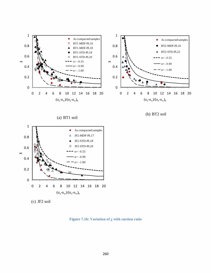
260

(a) BT1 soil

(b) BT2 soil

(c) JF2 soil

Figure 7.16: Variation of χ with suction ratio

0

0.2

0.4

0.6

0.8

1

0 2 4 6 8 10 12 14 16 18 20

χ

(ua-uw)/(ua-uw)b

As compacted samples

BT1-MDF-PL16

BT1-MDF-PL18

BT1-STD-PL18

BT1-STD-PL20

n= - 0.55

n= - 0.90

n= - 1.80

0

0.2

0.4

0.6

0.8

1

0 2 4 6 8 10 12 14 16 18 20

χ

(ua-uw)/(ua-uw)b


BT2-MDF-PL16

BT2-STD-PL22

n= - 0.55

n= - 0.90

n= - 1.80

0

0.2

0.4

0.6

0.8

1

0 2 4 6 8 10 12 14 16 18 20

χ

(ua-uw)/(ua-uw)b


JF2-MDF-PL17

JF2-STD-PL18

JF2-STD-PL20

n= - 0.55

n= - 0.90

n= - 1.80

261


This chapter has explored possibilities of applying conventional tests to obtain unsaturated shear

strength parameters. Although the chapter has been largely exploratory, the following issues

have been highlighted:

Stress history, suction, void ratio and structure have great influence on the shear strength

behavior of unsaturated soils. The influence of strain rate was not investigated in this study.

However, it is envisaged that strain rate has an important influence on the observations and needs

to be studied.

In order to obtain meaningful saturated shear strength parameters from a CU test, it is important

that stress history of the soil is understood. Compacted soils possess a stress history which is

revealed by their stress-strain behavior.

In this study, variation of effective friction angle with dry density was not observed possibly due

to experimental errors. However, the variation of effective friction angle over the range of dry

density tested was small.

It seems possible to use UU test on unsaturated soils at low net confining stress to determine the

effective friction angle hence, CU test for such soils may not be necessary. This needs more

study.

The as-compacted soils provide lower values for tanϕb compared to dried soils and hence may

provide conservative tanϕb for design. It would be interesting to investigate behavior of

specimens tested as-compacted at a constant density with only variation in compaction water

content. In this study both dry density and compaction water content varied.

262

One set back of the present study is that matric suction of the specimen was not monitored

during shearing. Without matric suction measurements, observations into the soil behavior are

limited and some assumptions are needed. However, this study presents a possible way of

interpreting a CW shear test for unsaturated soil test which is fast and possibly applicable in

practice. It is recommended that the observations be validated with suction monitoring during

shearing.

263

8. Conclusion and Recommendations

This study explores simple, economical and accessible means of obtaining unsaturated soil

properties with a motivation to apply unsaturated soil mechanics in practice. The main focus has

been on determination of suction, permeability and shear strength of compacted soils. Below are

the conclusion and recommendations for the study.

8.1 Conclusions

8.1.1 Suction measurements

The filter paper technique has been the main focus of suction measurement owing to its

affordability, ease of use and capacity to measure a wide range of suction. Both the initially dry

and initially wet filter papers were studied as possible suction sensors. The study concluded that:

Although not much field data exists on using filter paper technique, the technique is still very

valuable for suction measurement especially if a strict protocol is observed. The initially dry

filter paper was found to be preferable to the initially wet filter paper in terms of shorter

equilibration time. The hypothesis that an initially wet filter paper may reduce equilibration time

was not supported by experimental data

The study agrees with previous studies that 1000 kPa is an appropriate boundary between the

low and high suction ranges for practical applications. The contact filter paper is best suited for

low suction range while the non-contact one is best for the high suction range. This observation

has been corroborated by equilibration durations for the two contact modes of measurement.

Comparing suction measurements using the filter paper method on the as-compacted soil

specimens with suction readings from the SWCCs of the different specimens indicated good

264

agreement in the low suction range. The comparison in the higher suction range needs more

scrutiny through more studies

Good agreement was found between the suctions measured using the WP4C and the initially dry

contact filter paper. Since the WP4C is recommended as a benchmark for other techniques, this

observation is very positive for the filter paper method.

Comparison of the weight distributions of used and unused filter papers show that the used filter

papers have a slightly wider weight distribution than the unused filter papers. There is negligible

difference in weight distributions between the contact and non-contact filter papers indicating

that contamination of filter paper is not an issue and hence, there may not be a need to use

sacrificial filter papers in the contact filter paper method to prevent contamination of the filter

paper.

8.1.2 Permeability measurements

The suitability of a mini-disk infiltrometer in measuring near-saturated permeabilities of soils has

been investigated using measurements from the flexible wall permeameter as the benchmark. It

was observed that:

Structure and void ratio influence the permeability of soils.

Permeabilities from the mini-disk infiltrometer are reliable and can give fast indications of the

surface infiltration characteristics of the ground. It is greatly preferred to obtain parameters from

SWCC measurements to compute the permeability from the infiltrometer test results, however

usage of empirical parameters has proved useful and can be relied on as first level estimate of

permeability.

265

As the tension infiltrometers eliminate the effect of macroporosity, they are very valuable in

studying rain infiltration which too is largely influenced by the soil matrix and not the

macropores.

Better estimates of permeability are obtained for dry soils compared to wet soils. This further re-

in forces the usefulness of a disk infiltrometer as a tool to measure permeability.

8.1.3 Unconfined compressive strength and tensile strength

Studies of the unconfined compressive strength and tensile strength of compacted soils revealed

that:

There is an interplay of matric suction, soil structure and void ratio influencing soil strength. As

soils dry, the influence of matric suction on strength becomes increasingly minimal past the air-

entry value, the contribution is negligible as the water phase becomes increasingly gets

discontinuous. This is valuable in designing shear strength experiments for unsaturated soils.

The unconfined compressive strength for a near saturated soil as it dries increases up to the

shrinkage limit. Hence, shrinkage limit which indicates no further change in void ratio is an

important water content in strength of unsaturated soils.

The ratio of unconfined compressive strength to Brazilian tensile strength (qu/σt) lies within the

range of 4 to 15.

The two tensile strength models evaluated were not able to capture the tensile strength of the

compacted soils studied indicating complexity of the soil structure for compacted soils.

266

8.1.4 Constant water content tests

Possibilities of applying conventional tests to obtain unsaturated shear strength parameters have

been explored. A conventional triaxial apparatus was used to conduct UC and UU tests for as-

compacted soil specimens as well as the CU tests on the saturated soil specimens. The main

findings are listed below.

Stress history, suction, void ratio and structure have great influence on the shear strength

behavior of unsaturated and saturated soils. Compacted soils possess a stress history which needs

to be studied to have a better understanding on their shear strength measurements.

By fitting tangent lines inclined at effective friction angle to the Mohr circles from UC and UU

tests, shear strength of unsaturated soils can be obtained. This seems valuable especially for dry

of optimum soils which behave like OC clays. The results indicate that it may even be possible to

estimate the effective friction angle and hence conventional CU test may not be necessary for

such soils. However, this needs further exploration.

The as-compacted soils provide the lower tanϕb values than the dried soils and hence are useful

for determining design values necessary for conservative design in unsaturated soils.

8.2Recommendations

Not all issues were satisfactorily studied in this thesis. The following recommendations are made

for future study:

1) A lot of success has been recorded on the usage of filter paper method in laboratory

measurements of soil suction. Few measurements exist on field soil samples thus limiting

its application. In order to extend its use into practice, it is necessary to do more suction

267

measurements on field soil specimens using the filter paper method. Such experience will

be valuable for practitioners.

2) The effect of the sacrificial filter paper recommended by ASTM D-5298-16 on

equilibration time of filter papers needs to be further investigated as the current study

shows that it is not needed.

3) Infiltrometers with larger disk diameters need to be studied further and their advantages

over mini-disks in terms of reliability of results be further investigated.

4) More studies are needed on how to obtain reliable permeabilities for wet soils using mini-

disk infiltromters considering spatial variability of soils.

5) In this thesis, infiltration studies were done on compacted soils. It would be interesting to

investigate the reliability of Carsel and Parrish (1988) empirical parameters on natural

soils and compare with actual SWCC measurements. If found reliable, the duration of

permeability measurements with a disk infiltrometer would be further shortened for

practice.

6) More studies of UCS and BTS are necessary to establish ways of obtaining reliable

unsaturated shear strength parameters in a short time. Studies relating UCS and BTS have

been done in stabilized materials but do not seem to align with unsaturated soil

mechanics principles. This needs to be studied. Also, the linkage between BTS and the

SWCC of soils needs more investigation especially for soils with complex structures such

as compacted soils.

7) The tensile strength models evaluated in this study indicates that there is a need to

develop a new model to estimate tensile strength of compacted soils.

268

8) Initial stress state of compacted soils needs to be established in order to gain more

understanding of the shear strength tests of these soils.

9) The framework of the CW test presented in Chapter 7 is very promising and needs to be

investigated further on different soils especially soils with high matric suctions.

Measurements such as volume change during shear, suction changes during shearing are

necessary to validate the observations and assumptions made. The influence of strain rate

on the observations also needs to be studied.

269

References

ASTM D698-12. Standard Test Methods for Laboratory Compaction Characteristics of Soil Using Standard Effort (12 400 ft-lbf/ft3 (600 kN-m/m3)), ASTM International. West Conshohocken, PA 2012, www.astm.org.

ASTM D854-14. Standard Test Methods for Specific Gravity of Soil Solids by Water Pycnometer, ASTM International. West Conshohocken, PA 2014, www.astm.org.

ASTM D2166 / D2166M - 16. Standard Test Method for Unconfined Compressive Strength of Cohesive Soil, ASTM International. West Conshohocken, PA 2016, www.astm.org.

ASTM D2216-10. Standard Test Methods for Laboratory Determination of Water (Moisture) Content of Soil and Rock by Mass. West Conshohocken, PA 2010, www.astm.org.

ASTM D2487-17. Standard Practice for Classification of Soils for Engineering Purposes (Unified Soil Classification System), ASTM International. West Conshohocken, PA 2017, www.astm.org.

ASTM D2850-15. Standard Test Method for Unconsolidated-Undrained Triaxial Compression Test on Cohesive Soils, ASTM International. West Conshohocken, PA 2015, www.astm.org.

ASTM D3967 - 16. Standard Test Method for Splitting Tensile Strength of Intact Rock Core Specimens, ASTM International. West Conshohocken, PA 2016, www.astm.org.

ASTM D4318-17. Standard Test Methods for Liquid Limit, Plastic Limit, and Plasticity Index of Soils, ASTM International West Conshohocken, PA 2017, www.astm.org.

ASTM D4767-11. Standard Test Method for Consolidated Undrained Triaxial Compression Test for Cohesive Soils. West Conshohocken, PA 2011, www.astm.org.

ASTM D5084 − 16a. Standard Test Methods for Measurement of Hydraulic Conductivity of Saturated Porous Materials Using a Flexible Wall Permeameter, ASTM International. West Conshohocken, PA 2016, www.astm.org.

ASTM D5298-16. Standard Method for Measurement of Soil Potential (Suction) Using Filter Paper, ASTM International. West Conshohocken, PA 2016, www.astm.org.

ASTM D5856 − 15. Standard Test Method for Measurement of Hydraulic Conductivity of Porous Material Using a Rigid-Wall, Compaction-Mold Permeameter, ASTM International. West Conshohocken, PA 2015, www.astm.org.

ASTM D6836 - 16. Standard Test Methods for Determination of the Soil Water Characteristic Curve for Desorption Using Hanging Column, Pressure Extractor, Chilled Mirror Hygrometer, or Centrifuge, ASTM International. West Conshohocken, PA 2016, www.astm.org.

ASTM D6913/D6913M-17. Standard Test Methods for Particle-Size Distribution (Gradation) of Soils Using Sieve Analysis. West Conshohocken, PA 2017, www.astm.org.

ASTM D7664-10. Standard Test Methods for Measurement of Hydraulic Conductivity of Unsaturated Soil, ASTM International. West Conshohocken, PA 2010, www.astm.org.

ASTM D7928-17. Standard Test Method for Particle-Size Distribution (Gradation) of Fine-Grained Soils Using the Sedimentation (Hydrometer) Analysis, ASTM International West Conshohocken, PA 2017, www.astm.org.

Decagon Devices (2014). Mini disk infi ltrometer: Model S, user’s manual version 3. Decagon Devices, Pullman, WA.

ACIKEL, A., SINGH, R., BOUAZZA, A., GATES, W. & ROWE, R. 2015. Applicability and accuracy of the initially dry and initially wet contact filter paper tests for matric suction measurement of geosynthetic clay liners. Geotechnique: international journal of soil mechanics, 65, 780-787.

AGUS, S., LEONG, E. & SCHANZ, T. 2003. Assessment of statistical models for indirect determination of permeability functions from soil–water characteristic curves. Géotechnique, 53, 279-282.

270

AGUS, S. S., LEONG, E. C. & RAHARDJO, H. 2001. Soil—water characteristic curves of Singapore residual soils. Unsaturated soil concepts and their application in geotechnical practice. Springer.

AGUS, S. S. & SCHANZ, T. 2005. Comparison of four methods for measuring total suction. Vadose Zone Journal, 4, 1087-1095.

AHMED, S., LOVELL, C. W. & DIAMOND, S. 1974. Pore sizes and strength of a compacted clay. AITCHISON, G. D. 1964. Engineering concepts of moisture equilibria and moisture changes in soils.

Statement of the Review Panel , In Moisture Equilibria and Moisture Changes in Soils Beneath Covered Areas. 7-21.

AKIN, I. D. & LIKOS, W. 2017. Brazilian Tensile Strength Testing of Compacted Clay. Geotechnical Testing Journal, 40, 608-617.

AL-KHAFAF, S. & HANKS, R. 1974. Evaluation of the filter paper method for estimating soil water potential. Soil Science, 117, 194-199.

ALONSO, E., PINYOL, N. & GENS, A. 2013. Compacted soil behaviour: initial state, structure and constitutive modelling. Géotechnique, 63, 463.

BAKER, R. & FRYDMAN, S. 2009. Unsaturated soil mechanics: Critical review of physical foundations. Engineering Geology, 106, 26-39.

BARBOUR, S. L. 1998. Nineteenth Canadian Geotechnical Colloquium: The soil-water characteristic curve: a historical perspective. Canadian Geotechnical Journal, 35, 873-894.

BARDEN, L. & PAVLAKIS, G. 1971. Air and water permeability of compacted unsaturated cohesive soil. Journal of Soil Science, 22, 302-318.

BENSON, C. & DANIEL, D. 1990. Influence of Clods on Hydraulic Conductivity of. BICALHO, K. V., CORREIA, A. G., FERREIRA, S. R., FLEUREAU, J.-M. & MARINHO, F. A. 2007. Filter paper

method of soil suction measurement. BICALHO, K. V., MARINHO, F. A., CORREIA, A. G., FERREIRA, S. R. & FLEUREAU, J.-M. 2008. Effect of the

filter paper calibration on the soil-water retention curve of an unsaturated compacted silt sand. BISHOP, A., ALPAN, I. & BLIGHT, G. Factors controlling the shear strenth of partly saturated cohesive soil.

ASCE Res. Conf. Shear Strength of Loheslve Soil. Univ. of Colordo, Boulder P, 1960. BISHOP, A. W. 1959. The principle of effective stress. Teknisk ukeblad, 39, 859-863. BISHOP, A. W. 1960. The principles of effective stress, Norges Geotekniske Institutt. BISHOP, A. W. & DONALD, I. The experimental study of partly saturated soil in the triaxial apparatus.

Proceedings of the 5th international conference on soil mechanics and foundation engineering, Paris, 1961. 13-21.

BJERRUM, L. & HUDER, J. Measurement of the permeability of compacted clays. Proceedings of the 4th international conference on soil mechanics and foundation engineering, London, 1957. 6-10.

BLATZ, J. A., CUI, Y.-J. & OLDECOP, L. 2008. Vapour equilibrium and osmotic technique for suction control. Laboratory and Field Testing of Unsaturated Soils. Springer.

BOSO, M., TARANTINO, A. & MONGIOVI, L. 2005. A direct shear box improved with the osmotic technique. Proceedings of advanced experimental unsaturated soil mechanics, Trento, 85-91.

BROOKS, R. H. & COREY, A. T. 1964. Hydraulic properties of porous media. Colorado State University, Hydrology Paper No.3, 3, 27.

BRUCE, R. & KLUTE, A. 1956. The Measurement of Soil Moisture Diffusivity 1. Soil Science Society of America Journal, 20, 458-462.

BUCKINGHAM, E. 1907. Studies on the movement of soil moisture. US Dept. Agic. Bur. Soils Bull., 38. BULUT, R. & LEONG, E. C. 2008. Indirect measurement of suction. Geotechnical and Geological

Engineering, 26, 633-644. BULUT, R., LYTTON, R. L. & WRAY, W. K. Soil suction measurements by filter paper. Expansive clay soils

and vegetative influence on shallow foundations, 2001. ASCE, 243-261.

271

BULUT, R. & WRAY, W. K. 2005. Free energy of water-suction-in filter papers. ASTM geotechnical testing journal, 28, 355-364.

BURDINE, N. 1953. Relative permeability calculations from pore size distribution data. Journal of Petroleum Technology, 5, 71-78.

BURLAND, J. 1965. Some Aspects of the Mechanical Behaviour of Party Saturated Soils. Moisture equilibria and moisture changes in soils beneath covered areas, 270-278.

CAMPBELL, G. S., SMITH, D. M. & TEARE, B. L. 2007. Application of a dew point method to obtain the soil water characteristic. Experimental Unsaturated Soil Mechanics. Springer.

CARMAN, P. C. 1956. Flow of gases through porous media. CARRIER III, W. D. 2003. Goodbye, hazen; hello, kozeny-carman. Journal of geotechnical and

geoenvironmental engineering, 129, 1054-1056. CARSEL, R. F. & PARRISH, R. S. 1988. Developing joint probability distributions of soil water retention

characteristics. Water resources research, 24, 755-769. CARUSO, M. & TARANTINO, A. 2004. A shearbox for testing unsaturated soils at medium to high degrees

of saturation. Géotechnique, 54. CHANDLER, R. & GUTIERREZ, C. 1986. The filter-paper method of suction measurement. Géotechnique,

36, 265-268. CHANG, C. & DUNCAN, J. 1983. Consolidation analysis for partly saturated clay by using an elastic–plastic

effective stress–strain model. International Journal for Numerical and Analytical Methods in Geomechanics, 7, 39-55.

CHANG, C. S. 1976. Analysis of consolidation of earth and rockfill dams. Ph. D Thesis, University of California, 1-225.

CHAPUIS, R. 2017. Compacted Clay: Difficulties Obtaining Good Laboratory Permeability Tests. Geotechnical Testing Journal, 40, 185-198.

CHAPUIS, R. P. 2012. Predicting the saturated hydraulic conductivity of soils: a review. Bulletin of engineering geology and the environment, 71, 401-434.

CHAPUIS, R. P. & AUBERTIN, M. 2003. On the use of the Kozeny Carman equation to predict the hydraulic conductivity of soils. Canadian Geotechnical Journal, 40, 616-628.

CHENG, C. & CHEN, X. 2007. Evaluation of methods for determination of hydraulic properties in an aquifer–aquitard system hydrologically connected to a river. Hydrogeology Journal, 15, 669-678.

CHILDS, E. C. & COLLIS-GEORGE, N. 1950. The permeability of porous materials. Proc. R. Soc. Lond. A, 201, 392-405.

CLOTHIER, B. & WHITE, I. 1981. Measurement of Sorptivity and Soil Water Diffusivity in the Field 1. Soil Science Society of America Journal, 45, 241-245.

CUISINIER, O. & LALOUI, L. 2004. Fabric evolution during hydromechanical loading of a compacted silt. International Journal for Numerical and Analytical Methods in Geomechanics, 28, 483-499.

DANIEL, D. E. 1989. In situ hydraulic conductivity tests for compacted clay. Journal of Geotechnical Engineering, 115, 1205-1226.

DANIEL, D. E., ANDERSON, D. C. & BOYNTON, S. S. 1985. Fixed-wall versus flexible-wall permeameters. Hydraulic barriers in soil and rock. ASTM International.

DANIEL, D. E., TRAUTWEIN, S. J., BOYNTON, S. S. & FOREMAN, D. E. 1984. Permeability testing with flexible-wall permeameters. Geotechnical Testing Journal, 7, 113-122.

DARCY, H. 1856. Les fontaines publiques de la ville de Dijon, Victor Dalmont, Paris. The Flow of Homogeneous Fluids Through Porous Media.

DAS, B., YEN, S. & DASS, R. 1995. Brazilian tensile strength test of lightly cemented sand. Canadian Geotechnical Journal, 32, 166-171.

272

DE OLIVEIRA, O. M., LI, P., MARINHO, F. A. & VANAPALLI, S. K. 2016. Mechanical behaviour of a compacted residual soil of gneiss from Brazil under constant water content condition. Indian Geotechnical Journal, 46, 299-308.

DEKA, R., WAIRIU, M., MTAKWA, P., MULLINS, C., VEENENDAAL, E. & TOWNEND, J. 1995. Use and accuracy of the filter‐paper technique for measurement of soil matric potential. European Journal of Soil Science, 46, 233-238.

DELAGE, P., AUDIGUIER, M., CUI, Y.-J. & HOWAT, M. D. 1996. Microstructure of a compacted silt. Canadian Geotechnical Journal, 33, 150-158.

DELAGE, P. & CUI, Y. J. 2008. An evaluation of the osmotic method of controlling suction∗. Geomechanics and Geoengineering: An International Journal, 3, 1-11.

DELAGE, P., ROMERO, E. & TARANTINO, A. Recent developments in the techniques of controlling and measuring suction in unsaturated soils. Keynote Lecture, Proc. 1st Eur. Conf. on Unsaturated Soils, 2008. 33-52.

DEVICES , DECAGON. Mini disk infiltrometer user’s manual version 10 (Decagon Devices,Inc: Pullman, WA) 2013.

DINEEN, K. & BURLAND, J. A new approach to osmotically controlled oedometer testing. PROCEEDINGS OF THE FIRST INTERNATIONAL CONFERENCE ON UNSATURATED SOILS/UNSAT'95/PARIS/FRANCE/6-8 SEPTEMBER 1995. VOLUME 2, 1995.

DOHNAL, M., DUSEK, J. & VOGEL, T. 2010. Improving hydraulic conductivity estimates from minidisk infiltrometer measurements for soils with wide pore-size distributions. Soil Science Society of America Journal, 74, 804-811.

EL MOUNTASSIR, G. 2011. Behaviour of a collapsible structured unsaturated fill material. PhD thesis, University of Strathclyde.

ELRICK, D. & REYNOLDS, W. 1990. Ponded Infiltration from a Single Ring: I. Analysis of Steady Flow. Soil Science Society of America Journal SSSJD 4, 54.

ESCARIO, V. Swelling of soils in contact with water at a negative pressure. Proceedings of the 2nd international conference expansive clay soils, Texas A&M University, 1969. 207-217.

ESCARIO, V. 1986. The shear strength of partly saturated soils. Geotech, 36, 453-456. FAWCETT, R. & COLLIS-GEORGE, N. 1967. A filter-paper method for determining the moisture

characteristics of soil. Australian Journal of Experimental Agriculture, 7, 162-167. FLEUREAU, J.-M., VERBRUGGE, J.-C., HUERGO, P. J., CORREIA, A. G. & KHEIRBEK-SAOUD, S. 2002. Aspects

of the behaviour of compacted clayey soils on drying and wetting paths. Canadian geotechnical journal, 39, 1341-1357.

FREDLUND, MORGENSTERN & WIDGER 1978. The shear strength of unsaturated soils. Canadian Geotechnical Journal, 15, 313-321.

FREDLUND, D. Seepage in saturated soils. Panel Discussion: Ground water and seepage problems. Proc. 10 th Int. Conf. Soil Mech. Found. Eng. Estocolmo, Suecia, 1981. 629-641.

FREDLUND, D. Use of soil-water characteristic curves in the implementation of unsaturated soil mechanics. Proceedings of the 3rd International Conference on Unsaturated Soils, Recife, Brazil, 2002. 887-902.

FREDLUND, D. G. 1967. Comparison of soil suction and one-dimensional consolidation characteristics of a highly plastic clay, National Research Council Canada, Division of Building Research.

FREDLUND, D. G. 2000. The 1999 RM Hardy Lecture: The implementation of unsaturated soil mechanics into geotechnical engineering. Canadian Geotechnical Journal, 37, 963-986.

FREDLUND, D. G. 2006. Unsaturated soil mechanics in engineering practice. Journal of geotechnical and geoenvironmental engineering, 132, 286-321.

FREDLUND, D. G. & MORGENSTERN, N. R. 1977. Stress state variables for unsaturated soils. Journal of Geotechnical and Geoenvironmental Engineering, 103.

273

FREDLUND, D. G. & RAHARDJO, H. 1993. Soil mechanics for unsaturated soils, John Wiley & Sons. FREDLUND, D. G., RAHARDJO, H. & FREDLUND, M. D. 2012. Unsaturated soil mechanics in engineering

practice, John Wiley & Sons. FREDLUND, D. G. & XING, A. 1994. Equations for the soil-water characteristic curve. Canadian

geotechnical journal, 31, 521-532. FREDLUND, M. D., WILSON, G. W. & FREDLUND, D. G. 2002. Use of the grain-size distribution for

estimation of the soil-water characteristic curve. Canadian Geotechnical Journal, 39, 1103-1117. FRYDMAN, S. 1964. Applicability of the Brazilian (indirect tension) test to soils. FRYDMAN, S. & BAKER, R. 2009. Theoretical soil-water characteristic curves based on adsorption,

cavitation, and a double porosity model. International Journal of Geomechanics, 9, 250-257. GALLAGE, C. P. K. & UCHIMURA, T. 2010. Effects of dry density and grain size distribution on soil-water

characteristic curves of sandy soils. Soils and Foundations, 50, 161-172. GAN, J., FREDLUND, D. & RAHARDJO, H. 1988. Determination of the shear strength parameters of an

unsaturated soil using the direct shear test. Canadian Geotechnical Journal, 25, 500-510. GARDNER, R. 1937. A method of measuring the capillary tension of soil moisture over a wide moisture

range. Soil Science, 43, 277-284. GARDNER, W. 1956. Calculation of Capillary Conductivity from Pressure Plate Outflow Data 1. Soil

Science Society of America Journal, 20, 317-320. GARDNER, W. 1958. Some steady-state solutions of the unsaturated moisture flow equation with

application to evaporation from a water table. Soil science, 85, 228-232. GARVEN, E. & VANAPALLI, S. Evaluation of empirical procedures for predicting the shear strength of

unsaturated soils. Unsaturated Soils 2006, 2006a. ASCE, 2570-2592. GARVEN, E. & VANAPALLI, S. 2006b. Evaluation of empirical procedures for predicting the shear strength

of unsaturated soils. Unsaturated Soils 2006. GEE, G., CAMPBELL, M., CAMPBELL, G. & CAMPBELL, J. 1992. Rapid measurement of low soil water

potentials using a water activity meter. Soil Science Society of America Journal, 56, 1068-1070. GENS, A. 2010. Soil-environment interactions in geotechnical engineering. Géotechnique, 60, 3. GENS, A., SÁNCHEZ, M. & SHENG, D. 2006. On constitutive modelling of unsaturated soils. Acta

Geotechnica, 1, 137. GREACEN, E. 1960. Water content and soil strength. Journal of Soil Science, 11, 313-333. GREACEN, E., WALKER, G. & COOK, P. 1987. Evaluation of the filter paper method for measuring soil

water suction. HAGHIGHI, A., MEDERO, G. M., MARINHO, F. A., MERCIER, B. & WOODWARD, P. K. 2012. Temperature

effects on suction measurement using the filter paper technique. ASTM geotechnical testing journal, 35, 83-90.

HAMBLIN, A. 1981. Filter-paper method for routine measurement of field water potential. Journal of Hydrology, 53, 355-360.

HAVERKAMP, R., ROSS, P., SMETTEM, K. & PARLANGE, J. 1994. Three‐dimensional analysis of infiltration from the disc infiltrometer: 2. Physically based infiltration equation. Water Resources Research, 30, 2931-2935.

HAYASHI, M. & QUINTON, W. L. 2004. A constant-head well permeameter method for measuring field-saturated hydraulic conductivity above an impermeable layer. Canadian journal of soil science, 84, 255-264.

HAZEN, A. 1892. Some physical properties of sands and gravels: with special reference to their use in filtration, publisher not identified.

HEAD, K. H. 1998. Manual of soil laboratory testing, Volume 3: Efffective stress tests. Ed. 2, John Wiley and sons Ltd.

274

HEIBROCK, G., ZEH, R. & WITT, K. 2005. Tensile strength of compacted clays. Unsaturated soils: Experimental studies. Springer.

HILF, J. W. 1956. An investigation of pore water pressure in compacted cohesive soils. HO, D. Y. & FREDLUND, D. G. 1982. A multistage triaxial test for unsaturated soils. Geotechnical Testing

Journal, 5, 18-25. HOFFMANN, C., ROMERO, E. & ALONSO, E. Combining different controlled-suction techniques to study

expansive clays. Proceedings of the international symposium on advanced experimental unsaturated soils mechanics EXPERUS, Trento, Balkema, 2005. 61-67.

HOLTZ, R. D. & KOVACS, W. D. 1981. An introduction to geotechnical engineering. HOULSBY, G. 1997. The work input to an unsaturated granular material. Géotechnique, 47, 193-6. HUANG, S., FREDLUND, D. & BARBOUR, S. 1998. Measurement of the coefficient of permeability for a

deformable unsaturated soil using a triaxial permeameter. Canadian Geotechnical Journal, 35, 426-432.

JENNINGS, J. & BURLAND, J. 1962. Limitations to the use of effective stresses in partly saturated soils. Géotechnique, 12, 125-144.

JOTISANKASA, A., COOP, M. & RIDLEY, A. 2009. The mechanical behaviour of an unsaturated compacted silty clay. Géotechnique, 59, 415-428.

KASSIFF, G. & SHALOM, A. B. 1971. Experimental relationship between swell pressure and suction. Géotechnique, 21, 245-255.

KATO, S., YOSHIMURA, Y. & FREDLUND, D. G. Role of matric suction in the interpretation of unconfined compression tests In Proceedings of the Fifty-Eighth Canadian Geotechnical Conference, 2005.

KHALILI, N. & KHABBAZ, M. 1998. A unique relationship of chi for the determination of the shear strength of unsaturated soils. Geotechnique, 48.

KLUTE, A. 1965. Laboratory measurement of hydraulic conductivity of unsaturated soil. Methods of Soil Analysis. Part 1. Physical and Mineralogical Properties, Including Statistics of Measurement and Sampling, 253-261.

KLUTE, A. 1972. The determination of the hydraulic conductivity and diffusivity of unsaturated soils1. Soil Science, 113, 264-276.

KLUTE, A. & DIRKSEN, C. 1986. Hydraulic conductivity and diffusivity: Laboratory methods. Methods of soil analysis: part 1—physical and mineralogical methods, 687-734.

KOLIJI, A., LALOUI, L., CUSINIER, O. & VULLIET, L. 2006. Suction induced effects on the fabric of a structured soil. Transport in porous media, 64, 261-278.

KOZENY, J. 1927. Uber kapillare leitung der wasser in boden. Royal Academy of Science, Vienna, Proc. Class I, 136, 271-306.

KRISDANI, H., RAHARDJO, H. & LEONG, E.-C. 2009. Use of instantaneous profile and statistical methods to determine permeability functions of unsaturated soils. Canadian Geotechnical Journal, 46, 869-874.

KUNZE, R., UEHARA, G. & GRAHAM, K. 1968. Factors Important in the Calculation of Hydraulic Conductivity 1. Soil Science Society of America Journal, 32, 760-765.

LALOUI, L. 2013. Mechanics of unsaturated geomaterials, John Wiley & Sons. LAMBE, T. W. 1958. The engineering behavior of compacted clay. Journal of the Soil Mechanics and

Foundations Division, 84, 1-35. LAMBORN, M. J. 1986. A micromechanical approach to modeling partly saturated soils. Texas A&M

University. LEONG, E.-C., KIZZA, R. & RAHARDJO, H. Measurement of soil suction using moist filter paper. E3S Web

of Conferences, 2016. EDP Sciences, 10012. LEONG, E.-C., TRIPATHY, S. & RAHARDJO, H. 2003. Total suction measurement of unsaturated soils with

a device using the chilled-mirror dew-point technique. Geotechnique, 53, 173-182.

275

LEONG, E. 2019. Stress State Variables for Unsaturated Soils—Consensus and Controversy. Geotechnical Design and Practice. Springer.

LEONG, E. & RAHARDJO, H. Soil-water characteristic curves of compacted residual soils. Unsaturated soils. Proceedings of the 3rd international conference on unsaturated soils (UNSAT 2002), Recife, Brazil, 2002. 271-276.

LEONG, E., RAHARDJO, H. & TANG, S. Characterisation and engineering properties of Singapore residual soils. Proceedings of the International Workshop on Characterisation and Engineering Properties of Natural Soils, Singapore, December, 2002a. 2-4.

LEONG, E. & WIJAYA, M. 2015. Universal soil shrinkage curve equation. Geoderma, 237, 78-87. LEONG, E. C., HE, L. & RAHARDJO, H. 2002b. Factors affecting the filter paper method for total and

matric suction measurements. ASTM geotechnical testing journal, 25, 322-333. LEONG, E. C. & RAHARDJO, H. 1997a. Permeability functions for unsaturated soils. Journal of

Geotechnical and Geoenvironmental Engineering, 123, 1118-1126. LEONG, E. C. & RAHARDJO, H. 1997b. Review of soil-water characteristic curve equations. Journal of

geotechnical and geoenvironmental engineering, 123, 1106-1117. LI, Z.-S., FLEUREAU, J.-M. & TANG, L.-S. 2017. Aspects of compaction and drying–wetting curves of a

subgrade clayey soil. Géotechnique, 67, 1120-1126. LIKOS, W. J. 2000. Total suction-moisture content characteristics for expansive soils. Colorado School of

Mines. Arthur Lakes Library. LIKOS, W. J. & LU, N. 2002. Filter paper technique for measuring total soil suction. Transportation

Research Record: Journal of the Transportation Research Board, 1786, 120-128. LLORET, A. & ALONSO, E. 1980. Consolidation of unsaturated soils including swelling and collapse

behaviour. Géotechnique, 30, 449-477. LU, N., KIM, T.-H., STURE, S. & LIKOS, W. J. 2009. Tensile strength of unsaturated sand. Journal of

engineering mechanics, 135, 1410-1419. LU, N. & LIKOS, W. J. 2004. Unsaturated soil mechanics, Wiley. LU, Y.-F., LUO, X.-Q., WU, Y.-C. & CUI, Y. Study of fundamental properties of soil–water characteristic

curve. Proceedings of the 3rd Asian conference on unsaturated soils. Beijing: Science Press, 2007. 243-249.

MARINHO, F., AM , GONZALO CARNERO GUZMÁN, G. & DEL GAUDIO ORLANDO, P. 2016. Constant water content compression tests on unsaturated compacted soil with suction measurement using a HCT. International Journal of Geomechanics, 16, D4015008.

MARINHO, F. A. 2005. Nature of soil–water characteristic curve for plastic soils. Journal of geotechnical and geoenvironmental engineering, 131, 654-661.

MARINHO, F. A. & DA SILVA GOMES, J. E. 2011. The effect of contact on the filter paper method for measuring soil suction. Geotechnical testing journal, 35, 172-181.

MARINHO, F. A. & DA SILVA GOMES, J. E. 2012. The Effect of Contact on the Filter Paper Method for Measuring Soil Suction. ASTM geotechnical testing journal, 35, 172-181.

MARINHO, F. A. & OLIVEIRA, O. M. 2006. The filter paper method revisited. ASTM geotechnical testing journal, 29, 250-258.

MARINHO, F. A. & OLIVEIRA, O. M. 2012. Unconfined shear strength of compacted unsaturated plastic soils. Proceedings of the Institution of Civil Engineers-Geotechnical engineering, 165, 97-106.

MARSHALL, T. 1958. A relation between permeability and size distribution of pores. Journal of Soil Science, 9, 1-8.

MARSHALL, T. J., HOLMES, J. W. & ROSE, C. W. 1996. Soil physics, Cambridge University Press. MASROURI, F., BICALHO, K. V. & KAWAI, K. 2008. Laboratory hydraulic testing in unsaturated soils.

Geotechnical and Geological Engineering, 26, 691-704.

276

MCKEEN, R. Soil characterization using suction measurements. Proc., 25th Paving and Transportation Conf, 1988.

MCQUEEN, I. S. & MILLER, R. F. 1968. Calibration and evaluation of a wide-range gravimetric method for measuring moisture stress. Soil Science, 106, 225-231.

MEERDINK, J., BENSON, C. & KHIRE, M. 1996. Unsaturated hydraulic conductivity of two compacted barrier soils. Journal of geotechnical engineering, 122, 565-576.

MEILANI, I., RAHARDJO, H., LEONG, E.-C. & FREDLUND, D. G. 2002. Mini suction probe for matric suction measurements. Canadian Geotechnical Journal, 39, 1427-1432.

MENDES, J. 2011. Assessment of the impact of climate change on an instrumented embankment: An unsaturated soil mechanics approach PhD thesis, Durham University, Durham, U.K.

MILAN, V. & ANDJELKO, S. 1992. Determination of hydraulic conductivity of porous media from grain-size composition.

MIRZAII, A. & YASROBI, S. 2012. Influence of initial dry density on soil-water characteristics of two compacted soils. Geotechnique Letters, 2, 193-198.

MITCHELL, J. K. 1976. Fundamental of Soil Behaviour, John Wiley and Sons, New York. MITCHELL, J. K., HOOPER, D. R. & CAMPANELLA, R. G. 1966. Permeability of compacted clay. Journal of

Soil Mechanics & Foundations Div, 92. MONROY, R., ZDRAVKOVIC, L. & RIDLEY, A. 2009. Evolution of microstructure in compacted London Clay

during wetting and loading. Géotechnique, 60, 105-119. MORGENSTERN, N. Properties of compacted soils. Contribution to panel discussion, Session IV, Proc.,

6th Panamerican Conf. on Soil Mechanics and Foundation Engineering, 1979. 349-354. MUALEM, Y. 1976. A new model for predicting the hydraulic conductivity of unsaturated porous media.

Water resources research, 12, 513-522. MUALEM, Y. 1986. Hydraulic conductivity of unsaturated soils: prediction and formulas. Methods of Soil

Analysis: Part 1—Physical and Mineralogical Methods, 799-823. MUÑOZ-CASTELBLANCO, J., PEREIRA, J.-M., DELAGE, P. & CUI, Y.-J. Suction measurements on a natural

unsaturated soil: A reappraisal of the filter paper method. Unsaturated Soils-Proc. Fifth Int. Conf. on Unsaturated Soils, 2010. 707-712.

NARAIN, J. & RAWAT, P. C. 1970. Tensile strength of compacted soils. Journal of Soil Mechanics & Foundations Div.

ÖBERG, A.-L. & SÄLLFORS, G. 1997. Determination of shear strength parameters of unsaturated silts and sands based on the water retention curve. ASTM geotechnical testing journal, 20, 40-48.

ODONG, J. 2007. Evaluation of empirical formulae for determination of hydraulic conductivity based on grain-size analysis. Journal of American Science, 3, 54-60.

OH, W. T. 2012. Simple techniques for the implementation of the mechanics of unsaturated soils into engineering practice. PhD, University of Ottawa.

OLSON, R. & DANIEL, D. 1981. Measurement of the hydraulic conductivity of fine-grained soils. Permeability and groundwater contaminant transport. ASTM International.

PHILIP, J. R. 1957. The theory of infiltration: 4. Sorptivity and algebraic infiltration equations. Soil science, 84, 257-264.

PINTADO, X., LLORET, A. & ROMERO, E. 2009. Assessment of the use of the vapour equilibrium technique in controlled-suction tests. Canadian Geotechnical Journal, 46, 411-423.

PIRATHEEPAN, J., GNANENDRAN, C. & ARULRAJAH, A. 2012. Determination of c and φ from IDT and unconfined compression testing and numerical analysis. Journal of materials in civil engineering, 24, 1153-1164.

RAHARDJO, H., HENG, O. B. & CHOON, L. E. 2004. Shear strength of a compacted residual soil from consolidated drained and constant water content triaxial tests. Canadian Geotechnical Journal, 41, 421-436.

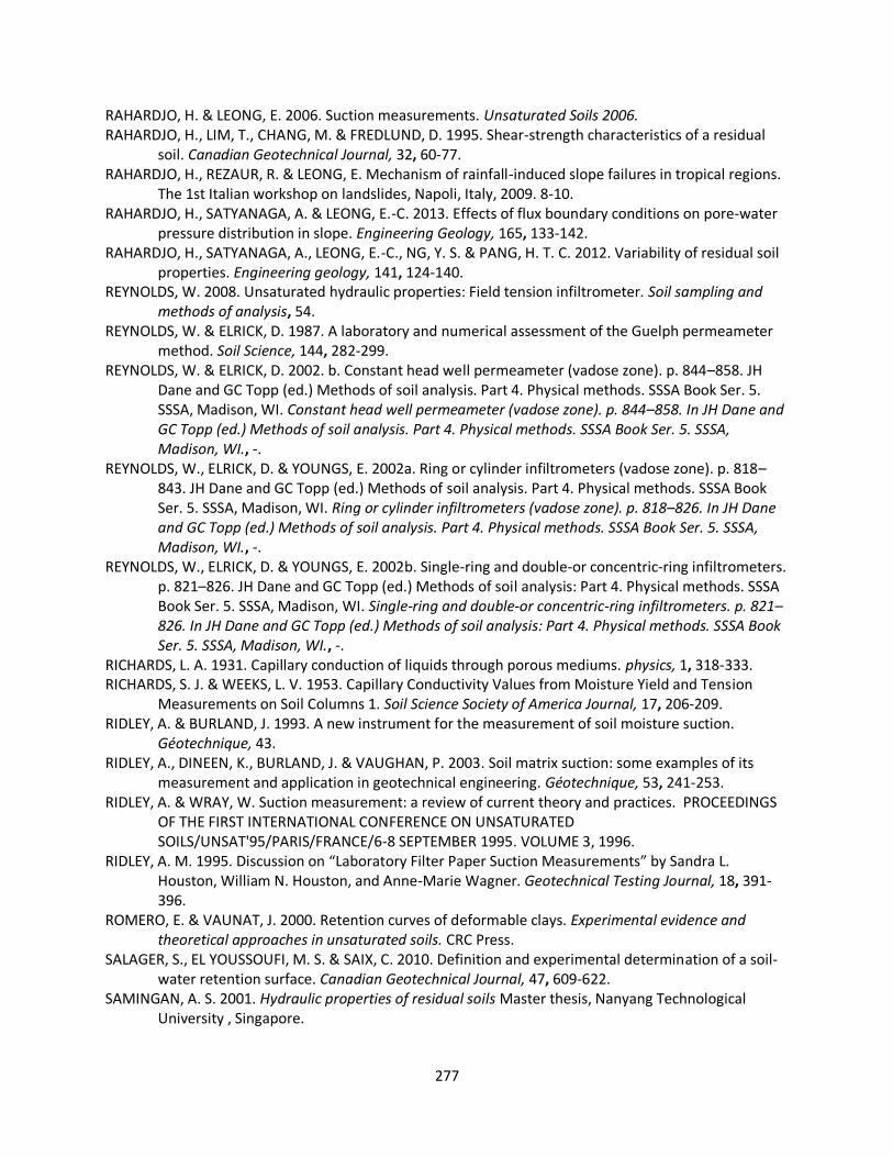
277

RAHARDJO, H. & LEONG, E. 2006. Suction measurements. Unsaturated Soils 2006. RAHARDJO, H., LIM, T., CHANG, M. & FREDLUND, D. 1995. Shear-strength characteristics of a residual

soil. Canadian Geotechnical Journal, 32, 60-77. RAHARDJO, H., REZAUR, R. & LEONG, E. Mechanism of rainfall-induced slope failures in tropical regions.

The 1st Italian workshop on landslides, Napoli, Italy, 2009. 8-10. RAHARDJO, H., SATYANAGA, A. & LEONG, E.-C. 2013. Effects of flux boundary conditions on pore-water

pressure distribution in slope. Engineering Geology, 165, 133-142. RAHARDJO, H., SATYANAGA, A., LEONG, E.-C., NG, Y. S. & PANG, H. T. C. 2012. Variability of residual soil

properties. Engineering geology, 141, 124-140. REYNOLDS, W. 2008. Unsaturated hydraulic properties: Field tension infiltrometer. Soil sampling and

methods of analysis, 54. REYNOLDS, W. & ELRICK, D. 1987. A laboratory and numerical assessment of the Guelph permeameter

method. Soil Science, 144, 282-299. REYNOLDS, W. & ELRICK, D. 2002. b. Constant head well permeameter (vadose zone). p. 844–858. JH

Dane and GC Topp (ed.) Methods of soil analysis. Part 4. Physical methods. SSSA Book Ser. 5. SSSA, Madison, WI. Constant head well permeameter (vadose zone). p. 844–858. In JH Dane and GC Topp (ed.) Methods of soil analysis. Part 4. Physical methods. SSSA Book Ser. 5. SSSA, Madison, WI., -.

REYNOLDS, W., ELRICK, D. & YOUNGS, E. 2002a. Ring or cylinder infiltrometers (vadose zone). p. 818–843. JH Dane and GC Topp (ed.) Methods of soil analysis. Part 4. Physical methods. SSSA Book Ser. 5. SSSA, Madison, WI. Ring or cylinder infiltrometers (vadose zone). p. 818–826. In JH Dane and GC Topp (ed.) Methods of soil analysis. Part 4. Physical methods. SSSA Book Ser. 5. SSSA, Madison, WI., -.

REYNOLDS, W., ELRICK, D. & YOUNGS, E. 2002b. Single-ring and double-or concentric-ring infiltrometers. p. 821–826. JH Dane and GC Topp (ed.) Methods of soil analysis: Part 4. Physical methods. SSSA Book Ser. 5. SSSA, Madison, WI. Single-ring and double-or concentric-ring infiltrometers. p. 821–826. In JH Dane and GC Topp (ed.) Methods of soil analysis: Part 4. Physical methods. SSSA Book Ser. 5. SSSA, Madison, WI., -.

RICHARDS, L. A. 1931. Capillary conduction of liquids through porous mediums. physics, 1, 318-333. RICHARDS, S. J. & WEEKS, L. V. 1953. Capillary Conductivity Values from Moisture Yield and Tension

Measurements on Soil Columns 1. Soil Science Society of America Journal, 17, 206-209. RIDLEY, A. & BURLAND, J. 1993. A new instrument for the measurement of soil moisture suction.

Géotechnique, 43. RIDLEY, A., DINEEN, K., BURLAND, J. & VAUGHAN, P. 2003. Soil matrix suction: some examples of its

measurement and application in geotechnical engineering. Géotechnique, 53, 241-253. RIDLEY, A. & WRAY, W. Suction measurement: a review of current theory and practices. PROCEEDINGS

OF THE FIRST INTERNATIONAL CONFERENCE ON UNSATURATED SOILS/UNSAT'95/PARIS/FRANCE/6-8 SEPTEMBER 1995. VOLUME 3, 1996.

RIDLEY, A. M. 1995. Discussion on “Laboratory Filter Paper Suction Measurements” by Sandra L. Houston, William N. Houston, and Anne-Marie Wagner. Geotechnical Testing Journal, 18, 391-396.

ROMERO, E. & VAUNAT, J. 2000. Retention curves of deformable clays. Experimental evidence and theoretical approaches in unsaturated soils. CRC Press.

SALAGER, S., EL YOUSSOUFI, M. S. & SAIX, C. 2010. Definition and experimental determination of a soil-water retention surface. Canadian Geotechnical Journal, 47, 609-622.

SAMINGAN, A. S. 2001. Hydraulic properties of residual soils Master thesis, Nanyang Technological University , Singapore.

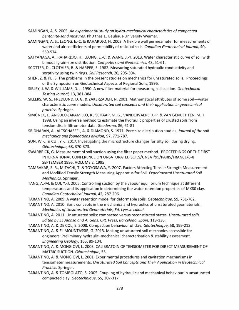
278

SAMINGAN, A. S. 2005. An experimental study on hydro-mechanical characteristics of compacted bentonite-sand mixtures. PhD thesis., Bauhaus-University Weimar.

SAMINGAN, A. S., LEONG, E.-C. & RAHARDJO, H. 2003. A flexible wall permeameter for measurements of water and air coefficients of permeability of residual soils. Canadian Geotechnical Journal, 40, 559-574.

SATYANAGA, A., RAHARDJO, H., LEONG, E.-C. & WANG, J.-Y. 2013. Water characteristic curve of soil with bimodal grain-size distribution. Computers and Geotechnics, 48, 51-61.

SCOTTER, D., CLOTHIER, B. & HARPER, E. 1982. Measuring saturated hydraulic conductivity and sorptivity using twin rings. Soil Research, 20, 295-304.

SHEN, Z. & YU, S. The problems in the present studies on mechanics for unsaturated soils. Proceedings of the Symposium on Geotechnical Aspects of Regional Soils, 1996.

SIBLEY, J. W. & WILLIAMS, D. J. 1990. A new filter material for measuring soil suction. Geotechnical Testing Journal, 13, 381-384.

SILLERS, W. S., FREDLUND, D. G. & ZAKERZADEH, N. 2001. Mathematical attributes of some soil—water characteristic curve models. Unsaturated soil concepts and their application in geotechnical practice. Springer.

ŠIMŮNEK, J., ANGULO-JARAMILLO, R., SCHAAP, M. G., VANDERVAERE, J.-P. & VAN GENUCHTEN, M. T. 1998. Using an inverse method to estimate the hydraulic properties of crusted soils from tension-disc infiltrometer data. Geoderma, 86, 61-81.

SRIDHARAN, A., ALTSCHAEFFL, A. & DIAMOND, S. 1971. Pore size distribution studies. Journal of the soil mechanics and foundations division, 97, 771-787.

SUN, W.-J. & CUI, Y.-J. 2017. Investigating the microstructure changes for silty soil during drying. Géotechnique, 68, 370-373.

SWARBRICK, G. Measurement of soil suction using the filter paper method. PROCEEDINGS OF THE FIRST INTERNATIONAL CONFERENCE ON UNSATURATED SOILS/UNSAT'95/PARIS/FRANCE/6-8 SEPTEMBER 1995. VOLUME 2, 1995.

TAMRAKAR, S. B., MITACHI, T. & TOYOSAWA, Y. 2007. Factors Affecting Tensile Strength Measurement and Modified Tensile Strength Measuring Apparatus for Soil. Experimental Unsaturated Soil Mechanics. Springer.

TANG, A.-M. & CUI, Y.-J. 2005. Controlling suction by the vapour equilibrium technique at different temperatures and its application in determining the water retention properties of MX80 clay. Canadian Geotechnical Journal, 42, 287-296.

TARANTINO, A. 2009. A water retention model for deformable soils. Géotechnique, 59, 751-762. TARANTINO, A. 2010. Basic concepts in the mechanics and hydraulics of unsaturated geomaterials. .

Mechanics of Unsaturated Geomaterials, Ed. Lyesse Laloui. TARANTINO, A. 2011. Unsaturated soils: compacted versus reconstituted states. Unsaturated soils.

Edited by EE Alonso and A. Gens. CRC Press, Barcelona, Spain, 113-136. TARANTINO, A. & DE COL, E. 2008. Compaction behaviour of clay. Géotechnique, 58, 199-213. TARANTINO, A. & EL MOUNTASSIR, G. 2013. Making unsaturated soil mechanics accessible for

engineers: Preliminary hydraulic–mechanical characterisation & stability assessment. Engineering Geology, 165, 89-104.

TARANTINO, A. & MONGIOVI, L. 2003. CALIBRATOIN OF TENSIOMETER FOR DIRECT MEASUREMENT OF MATRIC SUCTION. Géotechnique, 53.

TARANTINO, A. & MONGIOVÌ, L. 2001. Experimental procedures and cavitation mechanisms in tensiometer measurements. Unsaturated Soil Concepts and Their Application in Geotechnical Practice. Springer.

TARANTINO, A. & TOMBOLATO, S. 2005. Coupling of hydraulic and mechanical behaviour in unsaturated compacted clay. Géotechnique, 55, 307-317.

279

TAYLOR, D. 1948. Fundamentals of soil mechanics, Chapman And Hall, Limited.; New York. TERZAGHI, K. 1925. Erdbaumechanik auf bodenphysikalischer Grundlage. THU, T. M., RAHARDJO, H. & LEONG, E.-C. 2006. Shear strength and pore-water pressure characteristics

during constant water content triaxial tests. Journal of Geotechnical and Geoenvironmental Engineering, 132, 411-419.

TO-VIET, N., MIN, T.-K. & SHIN, H. 2013. Using inverse analysis to estimate hydraulic properties of unsaturated sand from one-dimensional outflow experiments. Engineering Geology, 164, 163-171.

TOLL, D., RAHARDJO, H. & LEONG, E. Landslides in Singapore. Proceedings of the 2nd International Conference on Landslides, Slope Stability and the Safety of Infra-Structures, Singapore, 1999. 27-28.

TULLER, M. & OR, D. 2005. Water films and scaling of soil characteristic curves at low water contents. Water Resources Research, 41.

TULLER, M., OR, D. & DUDLEY, L. M. 1999. Adsorption and capillary condensation in porous media: Liquid retention and interfacial configurations in angular pores. Water Resources Research, 35, 1949-1964.

VAN GENUCHTEN, M. T. 1980. A closed-form equation for predicting the hydraulic conductivity of unsaturated soils 1. Soil science society of America journal, 44, 892-898.

VANAPALLI, S. & FREDLUND, D. 2000. Comparison of different procedures to predict unsaturated soil shear strength. Geotechnical Special Publication, 195-209.

VANAPALLI, S., FREDLUND, D. & PUFAHL, D. 1999. The influence of soil structure and stress history on the soil–water characteristics of a compacted till. Geotechnique, 49, 143-159.

VANAPALLI, S., FREDLUND, D., PUFAHL, D. & CLIFTON, A. 1996a. Model for the prediction of shear strength with respect to soil suction. Canadian Geotechnical Journal, 33, 379-392.

VANAPALLI, S., SILLERS, W. & FREDLUND, M. The meaning and relevance of residual state to unsaturated soils. 51st Canadian Geotechnical Conference, 1998. sn, 4-7.

VANAPALLI, S. K. 1994. Simple test procedures and their interpretation in evaluating the shear strength of an unsaturated soil. . PhD thesis, University of Saskatchewan, Saskatoon.

VANAPALLI, S. K. 1995. Simple test procedures and their interpretation in evaluating the shear strength of an unsaturated soil.

VANAPALLI, S. K., FREDLUND, D. G. & PUFAHL, D. E. 1996b. The relationship between the soil-water characteristic curve and the unsaturated shear strength of a compacted glacial till. Geotechnical Testing Journal, 19, 259-268.

VANAPALLI, S. K., NICOTERA, M. & SHARMA, R. S. 2008. Axis translation and negative water column techniques for suction control. Laboratory and Field Testing of Unsaturated Soils. Springer.

WHEELER, S. 1988. A conceptual model for soils containing large gas bubbles. Geotechnique, 38, 389-397.

WHEELER, S., SHARMA, R. & BUISSON, M. 2003. Coupling of hydraulic hysteresis and stress–strain behaviour in unsaturated soils. Géotechnique, 53, 41-54.

WHITE, I. & SULLY, M. 1987. Macroscopic and microscopic capillary length and time scales from field infiltration. Water Resources Research, 23, 1514-1522.

WHITE, N. F., DUKE, H. R., SUNADA, D. K. & COREY, A. T. 1970. Physics of desaturation in porous materials. Journal of the Irrigation and Drainage Division, 96, 165-191.

WIJAYA, M. 2017. Compression, Shrinkage and Wetting-induced volume change of unsaturated soils. PhD thesis, Nanyang Technological Unviversity.

WIJAYA, M. & LEONG, E. C. 2017. Modelling the effect of density on the unimodal soil-water characteristic curve. Géotechnique, 67, 637-645.

280

WOODING, R. 1968. Steady infiltration from a shallow circular pond. Water resources research, 4, 1259-1273.

YANG, H., RAHARDJO, H., LEONG, E.-C. & FREDLUND, D. G. 2004. Factors affecting drying and wetting soil-water characteristic curves of sandy soils. Canadian Geotechnical Journal, 41, 908-920.

YIN, P. & VANAPALLI, S. K. 2018. Model for predicting tensile strength of unsaturated cohesionless soils. Canadian Geotechnical Journal, 55, 1313-1333.

YOUNG, J. F. 1967. Humidity control in the laboratory using salt solutions—a review. Journal of Applied Chemistry, 17, 241-245.

ZHAI, Q. & RAHARDJO, H. 2012. Determination of soil–water characteristic curve variables. Computers and Geotechnics, 42, 37-43.

ZHANG, R. 1997. Determination of soil sorptivity and hydraulic conductivity from the disk infiltrometer. Soil Science Society of America Journal, 61, 1024-1030.

ZHOU, A., SHENG, D. & CARTER, J. P. 2012. Modelling the effect of initial density on soil-water characteristic curves. Géotechnique, 62, 669-680.

281

APPENDICES

282

Appendix A-Suction and SWCC data

Contains Appendices A1-A5 (referenced in Chapter 4)

283

Appendix A1

a) Contact filter paper

b) Non-contact filter paper

Figure A1-1: Effect of equilibrium time on filter paper water content for standard Proctor compacted BT1 soils – Plastic mold

and Method 2

0

20

40

60

80

100

120

0 10 20 30 40 50 60

Fil

ter

pap

er w

ate

r co

nte

nt,

%

ID-C-FP

IW-C-FP

w=10%

0 10 20 30 40 50 60

w=13%

0 10 20 30 40 50 60

Duration in days

w=15.5%

0 10 20 30 40 50 60

w=18%

0 10 20 30 40 50 60

w=20%

0

20

40

60

80

100

120

0 10 20 30 40 50 60

Fil

ter

pap

er w

ate

r co

nte

nt,

%

ID-NC-FP

IW-NC-FP

w=10%

0 10 20 30 40 50 60

w=13%

0 10 20 30 40 50 60

Duration in days

w=15.5%

0 10 20 30 40 50 60

w=18%

0 10 20 30 40 50 60

w=20%

284

Appendix A1



Figure A1-2: Effect of equilibrium time on filter paper water content for modified Proctor compacted BT1 soils – Plastic

mold and Method 2

0 10 20 30 40 50 60

ID-C-FP

IW-C-FP

w=9%

0 10 20 30 40 50 60

Duration in days

w=12%

0 10 20 30 40 50 60

w=16.5%

0 10 20 30 40 50 60

ID-NC-FP

IW-NC-FP

w=9%

0 10 20 30 40 50 60

Duration in days

w=12%

0 10 20 30 40 50 60

w=16.5%

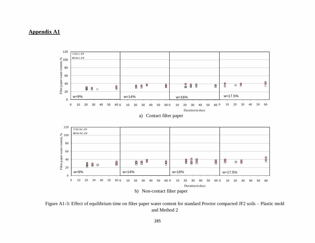
285

Appendix A1



Figure A1-3: Effect of equilibrium time on filter paper water content for standard Proctor compacted JF2 soils – Plastic mold

and Method 2

0

20

40

60

80

100

120

0 10 20 30 40 50 60

Fil

ter

pap

er w

ate

r co

nte

nt,

%

ID-C-FP

IW-C-FP

w=9%

0 10 20 30 40 50 60

w=14%

0 10 20 30 40 50 60

Duration in days

w=16%

0 10 20 30 40 50 60

w=17.5%

0

20

40

60

80

100

120

0 10 20 30 40 50 60

Fil

ter

pap

er w

ate

r co

nte

nt,

%

ID-NC-FP

IW-NC-FP

w=9%

0 10 20 30 40 50 60

w=14%

0 10 20 30 40 50 60

Duration in days

w=16%

0 10 20 30 40 50 60

w=17.5%

286

Appendix A1



Figure A1-4: Effect of equilibrium time on filter paper water content for modified Proctor compacted JF2 soils – Plastic mold

and Method 2

0

20

40

60

80

100

120

0 10 20 30 40 50 60

Fil

ter

pap

er w

ate

r co

nte

nt,

%

ID-C-FP

IW-C-FP

w=8%

0 10 20 30 40 50 60

Duration in days

w=12.5%

0 10 20 30 40 50 60

w=15%

0

20

40

60

80

100

120

0 10 20 30 40 50 60

Fil

ter

pap

er w

ate

r co

nte

nt,

%

ID-NC-FP

IW-NC-FP

w=8%

0 10 20 30 40 50 60

Duration in days

w=12.5%

0 10 20 30 40 50 60

w=15%

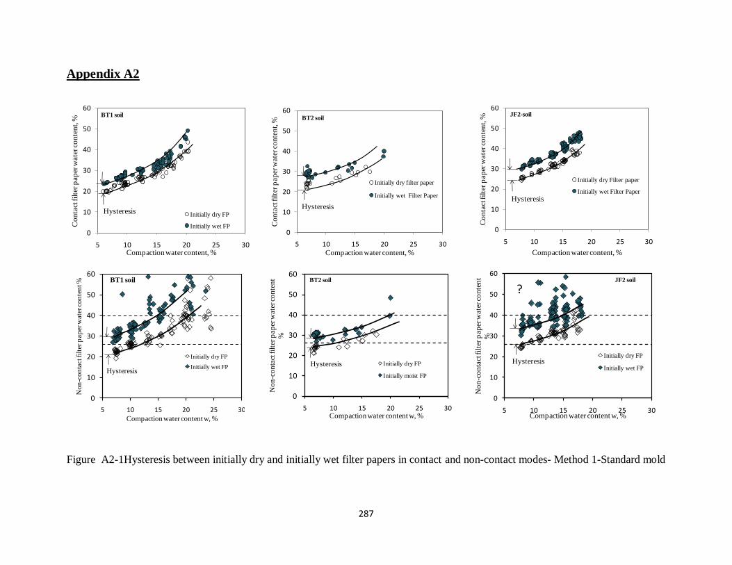
287

Appendix A2

Figure A2-1Hysteresis between initially dry and initially wet filter papers in contact and non-contact modes- Method 1-Standard mold

0

10

20

30

40

50

60

5 10 15 20 25 30

Co

nta

ct fil

ter

pap

er w

ate

r co

nte

nt,

%


Initially dry FP

Initially wet FP

Hysteresis

BT1 soil

0

10

20

30

40

50

60

5 10 15 20 25 30

Co

nta

ct fil

ter

pap

er w

ate

r co

nte

nt,

%



Initially wet Filter Paper

BT2 soil

Hysteresis

0

10

20

30

40

50

60

5 10 15 20 25 30

Co

nta

ct fil

ter

pap

er w

ate

r co

nte

nt,

%


Initially dry Filter paper

Initially wet Filter Paper

JF2-soil

Hysteresis

0

10

20

30

40

50

60

5 10 15 20 25 30

No

n-c

on

tact

fil

ter

pap

er w

ate

r co

nte

nt %


Initially dry FP

Initially wet FPHysteresis

BT1 soil

0

10

20

30

40

50

60

5 10 15 20 25 30

No

n-c

on

tact

fil

ter

pap

er w

ate

r co

nte

nt

%


Initially dry FP

Initially moist FP

Hysteresis

BT2 soil

0

10

20

30

40

50

60

5 10 15 20 25 30

No

n-c

on

tact

fil

ter

pap

er w

ate

r co

nte

nt

%


Initially dry FP

Initially wet FPHysteresis

?JF2 soil

288

Appendix A3

Figure A3-1: SWCC-w for BT1 standard Proctor specimens compacted in the standard

mold.

Figure A3-2: SWCC-w for BT1 modified Proctor specimens compacted in the standard

mold.

0

0.1

0.2

0.3

0.4

1 10 100 1000 10000 100000 1000000

Gra

vim

etri

c w

ate

r co

nte

nt

Suction, kPa

BT1-STD-ASTM10

BT1-STD-ASTM13

BT1-STD-ASTM16

BT1-STD-ASTM18

BT1-STD-ASTM20

BT1 soil

0

0.1

0.2

0.3

0.4

1 10 100 1000 10000 100000 1000000

Gra

vim

etri

c w

ate

r co

nte

nt

Suction, kPa

BT1-MDF-ASTM7

BT1-MDF-ASTM10

BT1-MDF-ASTM13

BT1-MDF-ASTM16

BT1-MDF-ASTM18

BT1 soil

289

Appendix A3

Figure A3-3: SWCC-w for BT2 standard Proctor specimens compacted in the standard

mold.

Figure A3-4: SWCC-w for BT2 modified Proctor specimens compacted in the standard

mold.

0

0.1

0.2

0.3

0.4

1 10 100 1000 10000 100000 1000000

Gra

vim

etri

c w

ate

r co

nte

nt

Suction, kPa

BT2-STD-ASTM13

BT2-STD-ASTM16

BT2-STD-ASTM19.5

BT2-STD-ASTM22

BT2 soil

0

0.1

0.2

0.3

0.4

1 10 100 1000 10000 100000 1000000

Gra

vim

etri

c w

ate

r co

nte

nt

Suction, kPa

BT2-MDF-ASTM8

BT2-MDF-ASTM11

BT2-MDF-ASTM13

BT2-MDF-ASTM15

BT2-MDF-ASTM16

BT2 soil

290

Appendix A3

Figure A3-5: SWCC-w for JF2 standard Proctor specimens compacted in the standard

mold.

Figure A3-6: SWCC-w for JF2 modified Proctor specimens compacted in the standard

mold.

0

0.1

0.2

0.3

0.4

1 10 100 1000 10000 100000 1000000

Gra

vim

etri

c w

ate

r co

nte

nt

Suction, kPa

JF2-STD-ASTM10

JF2-STD-ASTM14

JF2-STD-ASTM16

JF2-STD-ASTM18

JF2-STD-ASTM21

JF2 soil

0

0.1

0.2

0.3

0.4

1 10 100 1000 10000 100000 1000000

Gra

vim

etri

c w

ate

r co

nte

nt

Suction, kPa

JF2-MDF-ASTM8

JF2-MDF-ASTM11

JF2-MDF-ASTM13.5

JF2-MDF-ASTM15

JF2-MDF-ASTM17

JF2 soil

291

Appendix A3

Figure A3-7: SWCC-w for JF2 standard and modified Proctor specimens compacted in

the standard mold.

0

0.1

0.2

0.3

0.4

1 10 100 1000 10000 100000 1000000

Gra

vim

etri

c w

ate

r co

nte

nt

Suction, kPa

JF2-MDF-ASTM8

JF2-MDF-ASTM11

JF2-MDF-ASTM13.5

JF2-MDF-ASTM15

JF2-MDF-ASTM17

JF2-STD-ASTM10

JF2-STD-ASTM14

JF2-STD-ASTM16

JF2-STD-ASTM18

JF2-STD-ASTM21

JF2 soil

292

Appendix A4

Figure A4-1-SWCC-w for BT1 standard Proctor samples compacted in plastic

mold

Figure A4-2-SWCC-w for BT2 standard Proctor samples compacted in plastic

mold

0

0.1

0.2

0.3

0.4

1 10 100 1000 10000 100000 1000000

Gra

vim

etri

c w

ate

r co

nte

nt

Suction, kPa

BT1-STD-PL10

BT1-STD-PL13

BT1-STD-PL16

BT1-STD-PL18

BT1-STD-PL20

BT1 soil

0

0.1

0.2

0.3

0.4

1 10 100 1000 10000 100000 1000000

Gra

vim

etri

c w

ate

r co

nte

nt

Suction, kPa

BT2-STD-PL13

BT2-STD-PL16

BT2-STD-PL19.5

BT2-STD-PL22

293

Appendix A4

Figure A4-3-SWCC-w for JF1 standard Proctor samples compacted in plastic mol

Figure A4-4-SWCC-w for JF2 standard Proctor samples compacted in plastic mold

0

0.1

0.2

0.3

0.4

1 10 100 1000 10000 100000 1000000

Gra

vim

etri

c w

ate

r co

nte

nt,

%

Suction, kPa

JF1-STD-PL13

JF1-STD-PL18

JF1-STD-PL22

JF1 soil

0

0.1

0.2

0.3

0.4

1 10 100 1000 10000 100000 1000000

Gra

vim

etri

c w

ate

r co

nte

nt,

Suction, kPa

JF2-STD-PL10

JF2-STD-PL14

JF2-STD-PL16

JF2-STD-PL18

JF2-STD-PL21

JF2 soil

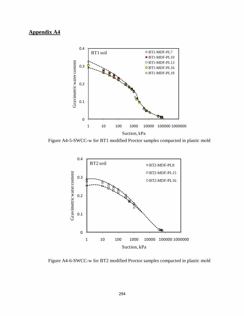
294

Appendix A4

Figure A4-5-SWCC-w for BT1 modified Proctor samples compacted in plastic mold

Figure A4-6-SWCC-w for BT2 modified Proctor samples compacted in plastic mold

0

0.1

0.2

0.3

0.4

1 10 100 1000 10000 100000 1000000

Gra

vim

etri

c w

ate

r co

nte

nt

Suction, kPa

BT1-MDF-PL7

BT1-MDF-PL10

BT1-MDF-PL13

BT1-MDF-PL16

BT1-MDF-PL18

BT1 soil

0

0.1

0.2

0.3

0.4

1 10 100 1000 10000 100000 1000000

Gra

vim

etri

c w

ate

r co

nte

nt

Suction, kPa

BT2-MDF-PL8

BT2-MDF-PL15

BT2-MDF-PL16

BT2 soil

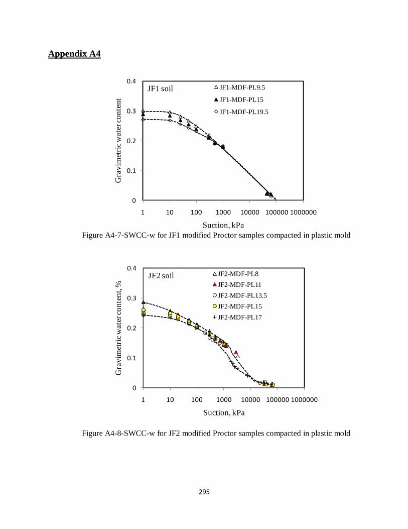
295

Appendix A4

Figure A4-7-SWCC-w for JF1 modified Proctor samples compacted in plastic mold

Figure A4-8-SWCC-w for JF2 modified Proctor samples compacted in plastic mold

0

0.1

0.2

0.3

0.4

1 10 100 1000 10000 100000 1000000

Gra

vim

etri

c w

ate

r co

nte

nt

Suction, kPa

JF1-MDF-PL9.5

JF1-MDF-PL15

JF1-MDF-PL19.5

JF1 soil

0

0.1

0.2

0.3

0.4

1 10 100 1000 10000 100000 1000000

Gra

vim

etri

c w

ate

r co

nte

nt,

%

Suction, kPa

JF2-MDF-PL8

JF2-MDF-PL11

JF2-MDF-PL13.5

JF2-MDF-PL15

JF2-MDF-PL17

JF2 soil

296

Appendix A4

Figure A4-9-SWCC-w for BT1 standard and modified Proctor samples compacted in

plastic mold

Figure A4-10-SWCC-w for JF2 standard and modified Proctor samples compacted in

plastic mold

0

0.1

0.2

0.3

0.4

1 10 100 1000 10000 100000 1000000

Gra

vim

etri

c w

ate

r co

nte

nt

Suction, kPa

BT1-MDF-PL7BT1-MDF-PL10BT1-MDF-PL13BT1-MDF-PL16BT1-MDF-PL18BT1-STD-PL10BT1-STD-PL13BT1-STD-PL16BT1-STD-PL18BT1-STD-PL20

BT1 soil

0

0.1

0.2

0.3

0.4

1 10 100 1000 10000 100000 1000000

Gra

vim

etri

c w

ate

r co

nte

nt,

%

Suction, kPa

JF2-MDF-PL8

JF2-MDF-PL11

JF2-MDF-PL13.5

JF2-MDF-PL15

JF2-MDF-PL17

JF2-STD-PL10

JF2-STD-PL14

JF2-STD-PL16

JF2-STD-PL18

JF2-STD-PL21

JF2 soil

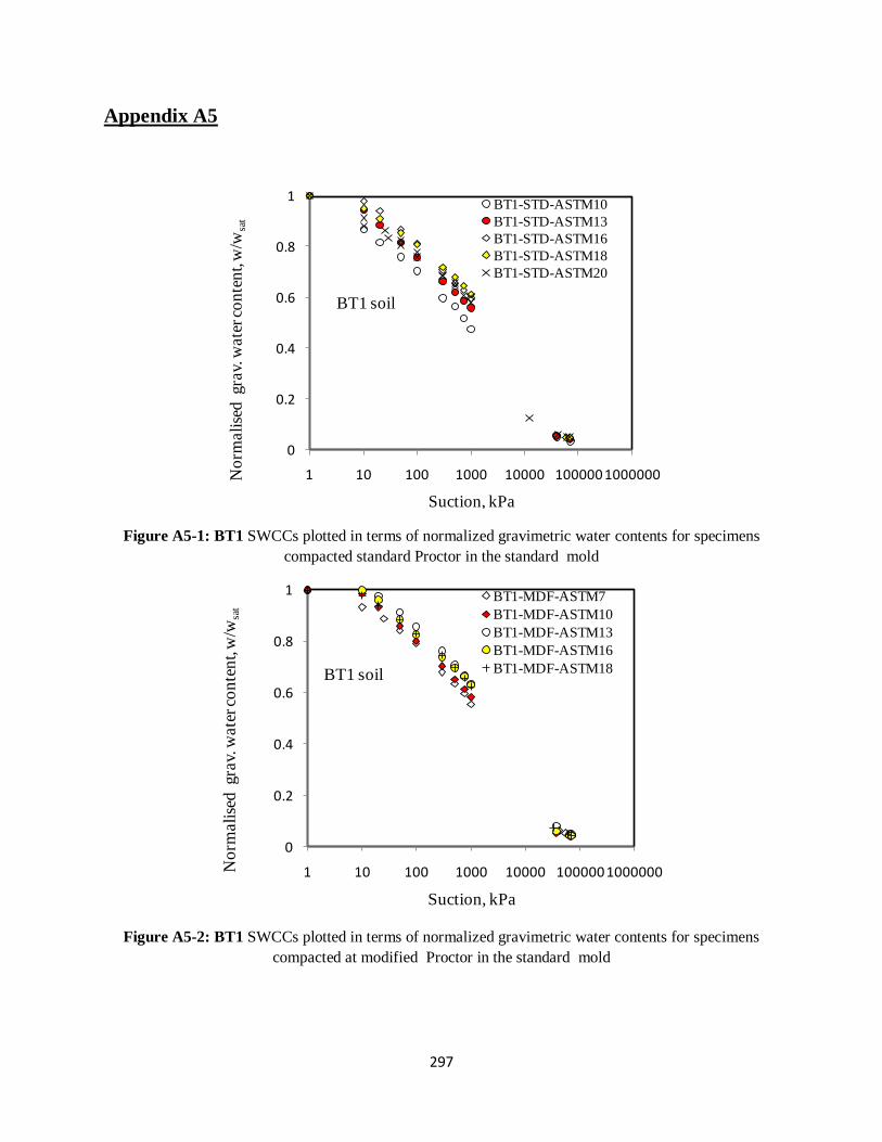
297

Appendix A5

Figure A5-1: BT1 SWCCs plotted in terms of normalized gravimetric water contents for specimens

compacted standard Proctor in the standard mold


compacted at modified Proctor in the standard mold

0

0.2

0.4

0.6

0.8

1

1 10 100 1000 10000 100000 1000000No

rmali

sed

gra

v. w

ate

r co

nte

nt, w

/wsa

t

Suction, kPa

BT1-STD-ASTM10

BT1-STD-ASTM13

BT1-STD-ASTM16

BT1-STD-ASTM18

BT1-STD-ASTM20

BT1 soil

0

0.2

0.4

0.6

0.8

1

1 10 100 1000 10000 1000001000000No

rmali

sed

gra

v. w

ate

r co

nte

nt, w

/wsa

t

Suction, kPa

BT1-MDF-ASTM7

BT1-MDF-ASTM10

BT1-MDF-ASTM13

BT1-MDF-ASTM16

BT1-MDF-ASTM18BT1 soil

298

Appendix A5


compacted at standard Proctor in the standard mold


compacted at modified Proctor in the standard mold

0

0.2

0.4

0.6

0.8

1

1 10 100 1000 10000 100000 1000000

No

rmali

sed

Gra

v. w

ate

r co

nte

nt,

w/w

sat

Suction, kPa

BT2-STD-ASTM13BT2-STD-ASTM16BT2-STD-ASTM19.5BT2-STD-ASTM22

BT2 soil

0

0.2

0.4

0.6

0.8

1

1 10 100 1000 10000 100000 1000000

No

rmali

sed

Gra

v. w

ate

r co

nte

nt,

w/w

sat

Suction, kPa

BT2-MDF-ASTM8

BT2-MDF-ASTM11

BT2-MDF-ASTM13

BT2-MDF-ASTM15

BT2-MDF-ASTM16

BT2 soil

299

Appendix A5

Figure A5-5: JF2 SWCCs plotted in terms of normalized gravimetric water contents for specimens




0

0.2

0.4

0.6

0.8

1

1 10 100 1000 10000 100000 1000000No

rmali

sed

Gra

v. w

ate

r co

nte

nt,

w/w

sat

Suction, kPa

JF2-STD-ASTM10

JF2-STD-ASTM14

JF2-STD-ASTM16

JF2-STD-ASTM18

JF2-STD-ASTM21

JF2 soil

0

0.2

0.4

0.6

0.8

1

1 10 100 1000 10000 100000 1000000

No

rmali

sed

Gra

v.w

ater

co

nte

nt,

w/w

sat

Suction, kPa

JF2-MDF-ASTM8

JF2-MDF-ASTM11

JF2-MDF-ASTM13.5

JF2-MDF-ASTM15

JF2-MDF-ASTM17JF2 soil

300

Appendix A5


compacted at both standard and modified Proctor in the standard mold

0

0.2

0.4

0.6

0.8

1

1 10 100 1000 10000 100000 1000000

No

rmali

sed

Gra

v. w

ate

r co

nte

nt,

w/w

s

Suction, kPa

BT2-MDF-ASTM8BT2-MDF-ASTM11BT2-MDF-ASTM13BT2-MDF-ASTM15BT2-MDF-ASTM16BT2-STD-ASTM13BT2-STD-ASTM16BT2-STD-ASTM19.5BT2-STD-ASTM22

BT2 soil

301

Appendix A5


compacted at standard Proctor in the plastic mold


compacted at modified Proctor in the plastic mold

0

0.2

0.4

0.6

0.8

1

1 10 100 1000 10000 100000 1000000No

rmali

sed

gra

v. w

ate

r co

nte

nt, w

/wsa

t

Suction, kPa

BT1-STD-PL10

BT1-STD-PL13

BT1-STD-PL16

BT1-STD-PL18

BT1-STD-PL20BT1 soil

0

0.2

0.4

0.6

0.8

1

1 10 100 1000 10000 100000 1000000No

rmali

sed

gra

v. w

ate

r co

nte

nt, w

/wsa

t

Suction, kPa

BT1-MDF-PL7

BT1-MDF-PL10

BT1-MDF-PL13

BT1-MDF-PL16

BT1-MDF-PL18BT1 soil

302

Appendix A5





0

0.2

0.4

0.6

0.8

1

1 10 100 1000 10000 100000 1000000No

rmali

sed

Gra

v.w

ater

co

nte

nt,

w/w

sat

Suction, kPa

BT2-STD-PL13

BT2-STD-PL16

BT2-STD-PL19.5

BT2-STD-PL22

BT2 soil

0

0.2

0.4

0.6

0.8

1

1 10 100 1000 10000 100000 1000000

No

rmali

sed

Gra

v.w

ater

co

nte

nt,

w/w

sat

Suction, kPa

BT2-MDF-PL8

BT2-MDF-PL15

BT2-MDF-PL16BT2 soil

303

Appendix A5





0

0.2

0.4

0.6

0.8

1

1 10 100 1000 10000 100000 1000000

No

rmali

sed

Gra

v.w

ater

co

nte

nt,

w/w

sat

Suction, kPa

JF1-STD-PL13

JF1-STD-PL18

JF1-STD-PL22

JF1 soil

0

0.2

0.4

0.6

0.8

1

1 10 100 1000 10000 100000 1000000

No

rmali

sed

Gra

v. w

ate

r co

nte

nt,

w/w

sat

Suction, kPa

JF1-MDF-PL9.5

JF1-MDF-PL15

JF1-MDF-PL19.5JF1 soil

304

Appendix A5





0

0.2

0.4

0.6

0.8

1

1 10 100 1000 10000 100000 1000000

No

rmali

sed

Gra

v. w

ate

r co

nte

nt,

w/w

sat

Suction, kPa

JF2-STD-PL10

JF2-STD-PL14

JF2-STD-PL16

JF2-STD-PL18

JF2-STD-PL21

JF2 soil

0

0.2

0.4

0.6

0.8

1

1 10 100 1000 10000 100000 1000000

No

rmali

sed

Gra

v. w

ate

r co

nte

nt,

w/w

sat

Suction, kPa

JF2-MDF-PL8

JF2-MDF-PL11

JF2-MDF-PL13.5

JF2-MDF-PL15

JF2-MDF-PL17

JF2 soil

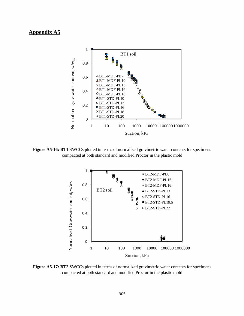
305

Appendix A5


compacted at both standard and modified Proctor in the plastic mold



0

0.2

0.4

0.6

0.8

1

1 10 100 1000 10000 100000 1000000No

rmali

sed

gra

v. w

ate

r co

nte

nt, w

/wsa

t

Suction, kPa

BT1-MDF-PL7

BT1-MDF-PL10

BT1-MDF-PL13

BT1-MDF-PL16

BT1-MDF-PL18

BT1-STD-PL10

BT1-STD-PL13

BT1-STD-PL16

BT1-STD-PL18

BT1-STD-PL20

BT1 soil

0

0.2

0.4

0.6

0.8

1

1 10 100 1000 10000 100000 1000000No

rmali

sed

Gra

v.w

ater

co

nte

nt,

w/w

s

Suction, kPa

BT2-MDF-PL8

BT2-MDF-PL15

BT2-MDF-PL16

BT2-STD-PL13

BT2-STD-PL16

BT2-STD-PL19.5

BT2-STD-PL22

BT2 soil

306

Appendix A5





0

0.2

0.4

0.6

0.8

1

1 10 100 1000 10000 100000 1000000

No

rmali

sed

Gra

v. w

ate

r co

nte

nt,

w/w

s

Suction, kPa

JF1-MDF-PL9.5

JF1-MDF-PL15

JF1-MDF-PL19.5

JF1-STD-PL13

JF1-STD-PL18

JF1-STD-PL22.8

JF1 soil

0

0.2

0.4

0.6

0.8

1

1 10 100 1000 10000 100000 1000000

No

rmali

sed

Gra

v. w

ate

r co

nte

nt,

w/w

sat

Suction, kPa

JF2-MDF-PL8

JF2-MDF-PL11

JF2-MDF-PL13.5

JF2-MDF-PL15

JF2-MDF-PL17

JF2-STD-PL10

JF2-STD-PL14

JF2-STD-PL16

JF2-STD-PL18

JF2-STD-PL21

JF2 soil

307

Appendix B-Hydraulic properties

Contains Appendices B1-B8 (Referenced to in Chapter 5)

308

Appendix B1: Flexible wall permeameter- Experimental runs for the

determination of ks

APPENDIX B1- BT1 soil sets

Experimental runs ks-values with run numbers

1

1.2

1.4

1.6

1.8

2

0 50000 100000 150000 200000

log

10h

t

time (s)

Run No.1

Run No.2

Run No.3

Run No.4

Run No.5

Run No.6

Run No.7

Run No.8

BT1-STD-ASTM10

1E-11

1E-10

1E-09

1E-08

1E-07

1E-06

1 2 3 4 5 6 7 8

k, m

/s

Run Number

BT1-STD-ASTM10

1.5

1.6

1.7

1.8

1.9

2

0 50000 100000 150000 200000

log

10h

t

time (s)

Run No.1

Run No.2

Run No.3

Run No.4

Run No.5

Run No.6

Run No.7

Run No.8

BT1-STD-ASTM13

1E-11

1E-10

1E-09

1E-08

1E-07

1E-06

1 2 3 4 5 6 7 8

k, m

/s

Run Number

BT1-STD-ASTM13

309

1.5

1.6

1.7

1.8

1.9

2

0 50000 100000 150000 200000

log

10h

t

time (s)

Run No.1

Run No.2

Run No.3

Run No.4

Run No.5

Run No.6

Run No.7

Run No.8

BT1-STD-ASTM16

1E-11

1E-10

1E-09

1E-08

1E-07

1E-06

1 2 3 4 5 6 7 8

k, m

/s

Run Number

BT1-STD-ASTM16

1.8

1.85

1.9

1.95

2

0 50000 100000 150000 200000

log

10h

t

time (s)

Run No.1

Run No.2

Run No.3

Run No.4

Run No.5

Run No.6

Run No.7

Run No.8

BT1-STD-ASTM18.3

1E-11

1E-10

1E-09

1E-08

1E-07

1E-06

1 2 3 4 5 6 7 8k

, m/s

Run Number

BT1-STD-ASTM18.3

1.5

1.6

1.7

1.8

1.9

2

0 50000 100000 150000 200000

log

10h

t

time (s)

Run No.1

Run No.2

Run No.3

Run No.4

Run No.5

Run No.6

Run No.7

Run No.8

BT1-STD-ASTM20.3

1E-11

1E-10

1E-09

1E-08

1E-07

1E-06

1 2 3 4 5 6 7 8

k, m

/s

Run Number

BT1-STD-ASTM20.3

310

1.5

1.6

1.7

1.8

1.9

2

0 50000 100000 150000 200000

log

10h

t

time (s)

Run No.1

Run No.2

Run No.3

Run No.4

BT1-MDF-ASTM7

1E-11

1E-10

1E-09

1E-08

1E-07

1E-06

1 2 3 4 5 6

k, m

/s

Run Number

BT1-MDF-ASTM7

1.8

1.85

1.9

1.95

2

0 50000 100000 150000 200000

log

10h

t

time (s)

Run No.1

Run No.2

Run No.3

Run No.4

BT1-MDF-ASTM10

1E-11

1E-10

1E-09

1E-08

1E-07

1E-06

1 2 3 4 5

k, m

/sRun Number

BT1-MDF-ASTM10

1.5

1.6

1.7

1.8

1.9

2

0 50000 100000 150000 200000

log

10h

t

time (s)

Run No.1

Run No.2

Run No.3

Run No.4

BT1-MDF-ASTM13

1E-11

1E-10

1E-09

1E-08

1E-07

1E-06

1 2 3 4 5

k, m

/s

Run Number

BT1-MDF-ASTM13

311

Appendix B1- BT2 soil sets

Experimental runs k-values with run numbers

1.8

1.85

1.9

1.95

2

0 50000 100000 150000 200000

log

10h

t

time (s)

Run No.1

Run No.2

Run No.3

Run No.4

Run No.5

BT1-MDF-ASTM16

1E-11

1E-10

1E-09

1E-08

1E-07

1E-06

1 2 3 4 5 6

k, m

/s

Run Number

BT1-MDF-ASTM16

1.5

1.6

1.7

1.8

1.9

2

0 50000 100000 150000 200000

log

10h

t

time (s)

Run No.1

Run No.2

Run No.3

Run No.4

Run No.5

BT1-MDF-ASTM17.8

1E-11

1E-10

1E-09

1E-08

1E-07

1E-06

1 2 3 4 5 6k

, m/s

Run Number

BT1-MDF-ASTM17.8

1.5

1.6

1.7

1.8

1.9

2

0 10000 20000 30000 40000 50000

log

10h

t

time (s)

Run No.1

Run No.2

Run No.3

Run No.4

Run No.6

Run No.7

Run No.8

BT2-STD-ASTM13

1E-11

1E-10

1E-09

1E-08

1E-07

1E-06

1 2 3 4 5 6 7 8 9

k, m

/s

Run Number

BT2-STD-ASTM13

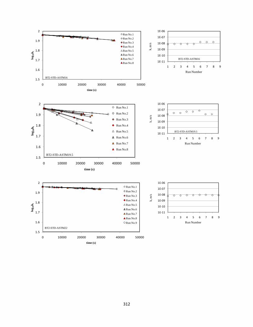
312

1.5

1.6

1.7

1.8

1.9

2

0 10000 20000 30000 40000 50000

log

10h

t

time (s)

Run No.1

Run No.2

Run No.3

Run No.4

Run No.5

Run No.6

Run No.7

Run No.8

BT2-STD-ASTM16

1E-11

1E-10

1E-09

1E-08

1E-07

1E-06

1 2 3 4 5 6 7 8 9

k, m

/s

Run Number

BT2-STD-ASTM16

1.5

1.6

1.7

1.8

1.9

2

0 10000 20000 30000 40000 50000

log

10h

t

time (s)

Run No.1

Run No.2

Run No.3

Run No.4

Run No.5

Run No.6

Run No.7

Run No.8

BT2-STD-ASTM19.5

1E-11

1E-10

1E-09

1E-08

1E-07

1E-06

1 2 3 4 5 6 7 8 9

k, m

/s

Run Number

BT2-STD-ASTM19.5

1.5

1.6

1.7

1.8

1.9

2

0 10000 20000 30000 40000 50000

log

10h

t

time (s)

Run No.1

Run No.2

Run No.3

Run No.4

Run No.5

Run No.6

Run No.7

Run No.8

Run No.9

BT2-STD-ASTM22

1E-11

1E-10

1E-09

1E-08

1E-07

1E-06

1 2 3 4 5 6 7 8 9

k, m

/s

Run Number

313

1.5

1.6

1.7

1.8

1.9

2

0 10000 20000 30000 40000 50000

log

10h

t

time (s)

Run No.1

Run No.2

Run No.3

Run No.4

Run No.5

Run No.6

Run No.7

Run No.8

Run No.9

BT2-MDF-ASTM8

1E-11

1E-10

1E-09

1E-08

1E-07

1E-06

1 2 3 4 5 6 7 8 9

k, m

/s

Run Number

BT2-MDF-ASTM8

1.5

1.6

1.7

1.8

1.9

2

0 10000 20000 30000 40000 50000

log

10h

t

time (s)

Run No.1

Run No.2

Run No.3

Run No.4

Run No.5

Run No.6

Run No.7

Run No.8

Run No.9BT2-MDF-ASTM11

1E-11

1E-10

1E-09

1E-08

1E-07

1E-06

1 2 3 4 5 6 7 8 9

k, m

/s

Run Number

BT2-MDF-ASTM11

1.5

1.6

1.7

1.8

1.9

2

0 10000 20000 30000 40000 50000

log

10h

t

time (s)

Run No.1

Run No.2

Run No.3

Run No.4

Run No.5

Run No.6

Run No.7

Run No.8

BT2-MDF-ASTM13

1E-11

1E-10

1E-09

1E-08

1E-07

1E-06

1 2 3 4 5 6 7 8

k, m

/s

Run Number

BT2-MDF-ASTM13

314

APPENDIX BT1- JF2 soil sets

Experimental runs k-values with run numbers

1.5

1.6

1.7

1.8

1.9

2

0 10000 20000 30000 40000 50000

log

10h

t

time (s)

Run No.1

Run No.2

Run No.3

Run No.4

Run No.5

Run No.6

Run No.7

Run No.8

BT2-MDF-ASTM14.7

1E-11

1E-10

1E-09

1E-08

1E-07

1E-06

1 2 3 4 5 6 7 8

k, m

/s

Run Number

BT2-MDF-ASTM 14.7

1.5

1.6

1.7

1.8

1.9

2

0 10000 20000 30000 40000 50000

log

10h

t

time (s)

Run No.1

Run No.2

Run No.3

Run No.4

Run No.5

Run No.6

Run No.7

Run No.8

BT2-MDF-ASTM16

1E-11

1E-10

1E-09

1E-08

1E-07

1E-06

1 2 3 4 5 6 7 8

k, m

/sRun Number

BT2-MDF-ASTM16

1.5

1.6

1.7

1.8

1.9

2

0 50000 100000 150000 200000

log

10h

t

time (s)

Run No.1

Run No.2

Run No.3

JF2-STD-ASTM10

1E-11

1E-10

1E-09

1E-08

1E-07

1E-06

1 2 3 4 5

k, m

/s

Run Number

JF2-STD-ASTM10

315

1.5

1.6

1.7

1.8

1.9

2

0 50000 100000 150000 200000

log

10h

t

time (s)

Run No.1

Run No.2

Run No.3

JF2-STD-ASTM14

1E-11

1E-10

1E-09

1E-08

1E-07

1E-06

1 2 3 4 5

k, m

/s

Run Number

JF2-STD-ASTM14

1.5

1.6

1.7

1.8

1.9

2

0 50000 100000 150000 200000

log

10h

t

time (s)

Run No.1

Run No.2

Run No.3

Run No.4

JF2-STD-ASTM16

1E-11

1E-10

1E-09

1E-08

1E-07

1E-06

1 2 3 4 5

k, m

/sRun Number

JF2-STD-ASTM16

1.5

1.6

1.7

1.8

1.9

2

0 50000 100000 150000 200000

log

10h

t

time (s)

Run No.1

Run No.2

Run No.3

JF2-STD-ASTM18

1E-11

1E-10

1E-09

1E-08

1E-07

1E-06

1 2 3 4 5

k, m

/s

Run Number

JF2-STD-ASTM18

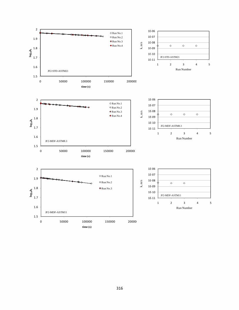
316

1.5

1.6

1.7

1.8

1.9

2

0 50000 100000 150000 200000

log

10h

t

time (s)

Run No.1

Run No.2

Run No.3

Run No.4

JF2-STD-ASTM21

1E-11

1E-10

1E-09

1E-08

1E-07

1E-06

1 2 3 4 5

k, m

/s

Run Number

JF2-STD-ASTM21

1.5

1.6

1.7

1.8

1.9

2

0 50000 100000 150000 200000

log

10h

t

time (s)

Run No.1

Run No.2

Run No.3

Run No.4

JF2-MDF-ASTM8.3

1E-11

1E-10

1E-09

1E-08

1E-07

1E-06

1 2 3 4 5

k, m

/sRun Number

JF2-MDF-ASTM8.3

1.5

1.6

1.7

1.8

1.9

2

0 50000 100000 150000 200000

log

10h

t

time (s)

Run No.1

Run No.2

Run No.3

JF2-MDF-ASTM11

1E-11

1E-10

1E-09

1E-08

1E-07

1E-06

1 2 3 4 5

k, m

/s

Run Number

JF2-MDF-ASTM11

317

1.5

1.6

1.7

1.8

1.9

2

0 50000 100000 150000 200000

log

10h

t

time (s)

Run No.1

Run No.2

Run No.3

Run No.4

JF2-MDF-ASTM13.5

1E-11

1E-10

1E-09

1E-08

1E-07

1E-06

1 2 3 4 5

k, m

/s

Run Number

JF2-MDF-ASTM13.5

1.5

1.6

1.7

1.8

1.9

2

0 50000 100000 150000 200000

log

10h

t

time (s)

Run No.1

Run No.2

Run No.3

JF2-MDF-ASTM15.4

1E-11

1E-10

1E-09

1E-08

1E-07

1E-06

1 2 3 4 5

k, m

/sRun Number

JF2-MDF-ASTM15.4

1.5

1.6

1.7

1.8

1.9

2

0 50000 100000 150000 200000

log

10h

t

time (s)

Run No.1

Run No.2

Run No.3

Run No.4

JF2-MDF-ASTM17

1E-11

1E-10

1E-09

1E-08

1E-07

1E-06

1 2 3 4 5

k, m

/s

Run Number

JF2-MDF-ASTM17

318

APPENDIX B2- Infiltration- time plots using the mini-disk infiltrometer

Dry of optimum (BT1 soil)

Wet of optimum (BT1 soil)

Figure B2-1: Infiltration-time plots for BT1 soil specimens

0

1

2

3

4

5

0 100 200 300 400 500

Cu

mm

ula

tive

infi

ltra

tio

n, (

cm)


BT1-STD-ASTM100

1

2

3

4

5

0 100 200 300 400 500

Cu

mm

ula

tive

infi

ltra

tio

n, (

cm)


BT1-STD-ASTM13

0

1

2

3

4

5

0 100 200 300 400 500

Cu

mm

ula

tive

infi

ltra

tio

n, (

cm)


BT1-MDF-ASTM7

0

1

2

3

4

5

0 100 200 300 400 500

Cu

mm

ula

tive

infi

ltra

tio

n, (

cm)


BT1-STD-ASTM180

1

2

3

4

5

0 100 200 300 400 500

Cu

mm

ula

tive

infi

ltra

tio

n, (

cm)


BT1-STD-ASTM200

1

2

3

4

5

0 100 200 300 400 500

Cu

mm

ula

tive

infi

ltra

tio

n, (

cm)


BT1-MDF-ASTM17.8

319

optimum

Figure B2-1: Infiltration-time plots for BT1 soil specimens

0

1

2

3

4

5

0 100 200 300 400 500

Cu

mm

ula

tive

infi

ltra

tio

n, (

cm)


BT1-STD-ASTM16

0

1

2

3

4

5

0 100 200 300 400 500

Cu

mm

ula

tive

infi

ltra

tio

n, (

cm)


BT1-MDF-ASTM13

0

1

2

3

4

5

0 100 200 300 400 500

Cu

mm

ula

tive

infi

ltra

tio

n, (

cm)


h = -1 cm

h = -2 cm

h = -5 cm

Legend

BT1-MDF-ASTM17.8

0

1

2

3

4

5

0 100 200 300 400 500

Cu

mm

ula

tive

infi

ltra

tio

n, (

cm)


BT1-MDF-ASTM160

1

2

3

4

5

0 100 200 300 400 500

Cu

mm

ula

tive

infi

ltra

tio

n, (

cm)


BT1-MDF-ASTM10

0

1

2

3

4

5

0 100 200 300 400 500

Cu

mm

ula

tive

infi

ltra

tio

n, (

cm)


BT2-STD-ASTM16

320

Figure B2-2: Infiltration-time plots for BT2 and JF2 soil specimens

0

1

2

3

4

5

0 100 200 300 400 500

Cu

mm

ula

tive

infi

ltra

tio

n, (

cm)


BT2-MDF-ASTM13

0

1

2

3

4

5

0 100 200 300 400 500

Cu

mm

ula

tive

infi

ltra

tio

n, (

cm)


BT2-MDF-ASTM15

0

1

2

3

4

5

0 100 200 300 400 500

Cu

mm

ula

tive

infi

ltra

tio

n, (

cm)


JF2-STD-ASTM14

0

1

2

3

4

5

0 100 200 300 400 500

Cu

mm

ula

tive

infi

ltra

tio

n, (

cm)


JF2-STD-ASTM16

0

1

2

3

4

5

0 100 200 300 400 500

Cu

mm

ula

tive

infi

ltra

tio

n, (

cm)


JF2-MDF-ASTM13.5

0

1

2

3

4

5

0 100 200 300 400 500

Cu

mm

ula

tive

infi

ltra

tio

n, (

cm)


JF2-MDF-ASTM15

321

APPENDIX B3: Infiltration equations for different soil sets at different suction pressure head

Appendix B3- Table B3-1: Infiltration equations with corresponding R2 for BT1 soil specimens at the different suction heads

BT1 soil sets Suction heads, cm

-1 -2 -5

STD-ASTM10 y=3E-4x2+0.0201x, R2= 0.999 y=2E-4x2+0.0109x, R2= 0.999 y=9E-5x2+0.0038x,

R2= 1


R2= 1

STD-ASTM16 y=2E-4x2+0.0074x, R2= 1 y=2E-4x2+0.0016x, R2= 1 y=7E-05x2+0.0015x,

R2= 0.999

STD-ASTM18 y=5E-05x2+0.0097x, R2= 1 y=7E-05x2+0.0033x, R2= 0.999 y=2E-05x2+0.003x,

R2= 0.999

STD-ASTM20 y=3E-05x2+0.0076x, R2= .999 y=2E-05x2+0.004x, R2= 0.999 y=1E-05x2+0.002x,

R2= 0.998

MDF-ASTM7 y=2E-4x2+0.0008x, R2= 0.999 y=1E-4x2+0.0087x, R2=0.999 y=1E-4x2+0.0073x,

R2= 0.999

MDF-ASTM10 y=7E-5x2+0.0105x, R2= 0.998 y=8E-5x2+0.0076x, R2= 0.999 y=4E-5x2+0.0023x,

R2= 0.999

MDF-ASTM13 y=5E-5x2+0.0089x, R2= 1 y=6E-5x2+0.0049x, R2= 0.999 y=2E-5x2+0.0035x,

R2= 0.999


R2= 0.999


R2= 0.998

322

Appendix B3- Table B3-2: Infiltration equations with corresponding R2 for BT2 soil specimens at the different suction heads

BT2 soil sets Suction heads, cm

-1 -2 -5


R2= 1


R2= 0.999

STD-ASTM19.5 y=2E-4x2+0.0082x, R2= 0.999 y=1E-4x2+0.0124x, R2= 0.998 y=9E-05x2+0.0051x,

R2= 0.999


R2= 0.999

MDF-ASTM8 y=4E-4x2+0.0193x, R2= 0.999 y=4E-4x2+0.0177x, R2=1 y=4E-4x2+0.016x,

R2= 0.999


R2= 0.999


R2= 0.999


R2= 0.992

MDF-ASTM16 y=8E-05x2+0.007x R2= 0.999 y=6E-05x2+0.007x, R2= 0.997 y=3E-05x2+0.006x,

R2= 0.999

323

Appendix B3- Table B3-3: Infiltration equations with corresponding R2 for JF2 soil specimens at the different suction heads

JF2 soil sets Suction heads, cm

-1 -2 -5

STD-ASTM10 y=2E-4x2+0.0142x, R2= 0.999 y=1E-4x2+0.006x, R2= 1 y=9E-5x2+0.005x,

R2= 0.999


R2= 1


R2= 1


R2= 0.997


R2= 0.996

MDF-ASTM8 y=1E-4x2+0.0077x, R2= 1 y=1E-4x2+0.0096x, R2=0.999 y=1E-4x2+0.0072x,

R2= 1


R2= 0.998

MDF-ASTM13.5 y=3E-5x2+0.0075x, R2= 0.999 y=2E-5x2+0.0058x, R2= 0.998 y=2E-5x2+0.0061x,

R2= 0.999


R2= 0.998


R2= 0.995

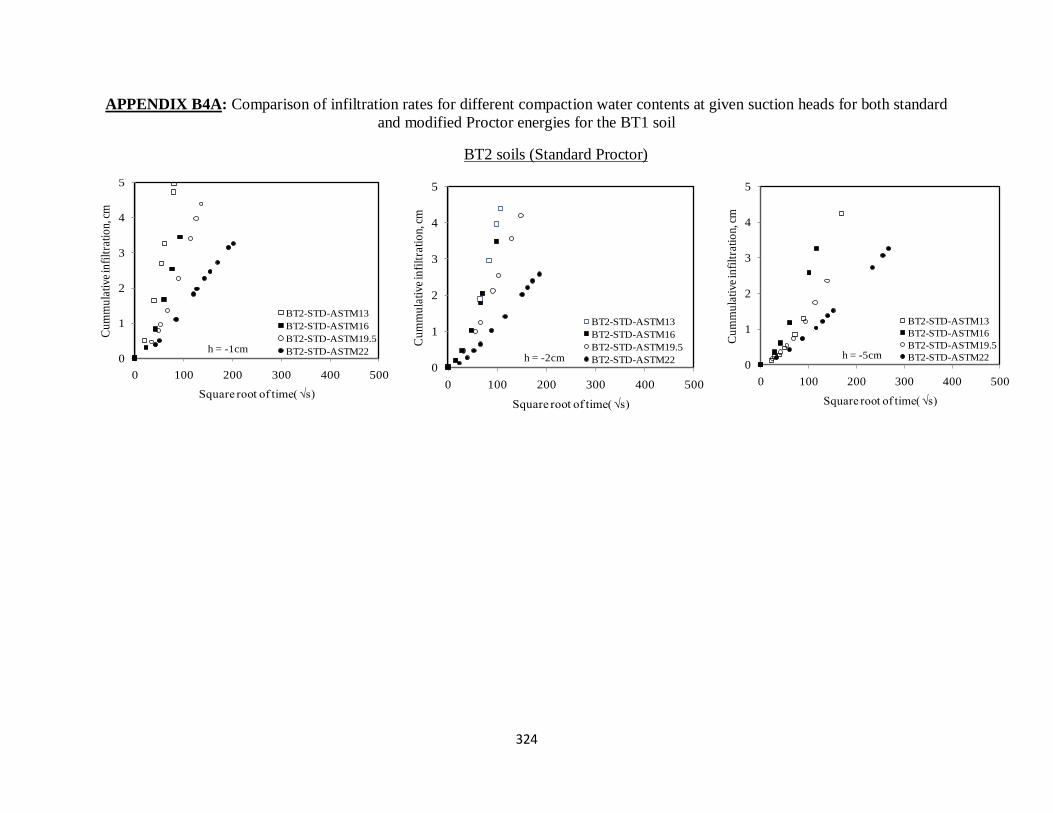
324

APPENDIX B4A: Comparison of infiltration rates for different compaction water contents at given suction heads for both standard

and modified Proctor energies for the BT1 soil

BT2 soils (Standard Proctor)

0

1

2

3

4

5

0 100 200 300 400 500

Cu

mm

ula

tive

infi

ltra

tio

n, c

m


BT2-STD-ASTM13

BT2-STD-ASTM16

BT2-STD-ASTM19.5

BT2-STD-ASTM22h = -1cm

0

1

2

3

4

5

0 100 200 300 400 500

Cu

mm

ula

tive

infi

ltra

tio

n, c

mSquare root of time( √s)

BT2-STD-ASTM13

BT2-STD-ASTM16

BT2-STD-ASTM19.5

BT2-STD-ASTM22h = -2cm0

1

2

3

4

5

0 100 200 300 400 500

Cu

mm

ula

tive

infi

ltra

tio

n, c

m


BT2-STD-ASTM13

BT2-STD-ASTM16

BT2-STD-ASTM19.5

BT2-STD-ASTM22h = -5cm

325

BT2 soils (modified Proctor)

Figure B4-1: Comparison of infiltration rates for different compaction water contents at given suction heads for both standard and

modified Proctor energies for the BT2 soil

0

1

2

3

4

5

0 100 200 300 400 500

Cu

mm

ula

tive

infi

ltra

tio

n, c

m


BT2-MDF-ASTM8BT2-MDF-ASTM11BT2-MDF-ASTM13BT2-MDF-ASTM15BT2-MDF-ASTM16h = -1cm

0

1

2

3

4

5

0 100 200 300 400 500

Cu

mm

ula

tive

infi

ltra

tio

n, c

m



0

1

2

3

4

5

0 100 200 300 400 500

Cu

mm

ula

tive

infi

ltra

tio

n, c

m



326

APPENDIX B4B:Comparison of infiltration rates for different compaction water contents at given suction heads for both standard

and modified Proctor energies


modified Proctor energies for the BT2 soil

0

1

2

3

4

5

0 100 200 300 400 500

Cu

mm

ula

tive

infi

ltra

tio

n, c

m


h = -1cm

BT2- soil specimens

0

1

2

3

4

5

0 100 200 300 400 500

Cu

mm

ula

tive

infi

ltra

tio

n, c

m


h = -2cm

BT2- soil specimens

0

1

2

3

4

5

0 100 200 300 400 500

Cu

mm

ula

tive

infi

ltra

tio

n, c

m


h = -5cm

BT2- soil specimens

0

1

2

3

4

5

0100200300400500

Cu

mm

ula

tive

infi

ltra

tio

n, c

m



BT2-STD-ASTM19.5 BT2-STD-ASTM22



BT2-MDF-ASTM16

h = -1cm

Legend (BT2):

327


modified Proctor energies for the JF2 soil

0

1

2

3

4

5

0 100 200 300 400 500

Cu

mm

ula

tive

infi

ltra

tio

n, c

m


h = -1cm

JF2 soil specimens

0

1

2

3

4

5

0 100 200 300 400 500

Cu

mm

ula

tive

infi

ltra

tio

n, c

m


h = -2cm

JF2 soil specimens

0

1

2

3

4

5

0 100 200 300 400 500

Cu

mm

ula

tive

infi

ltra

tio

n, c

m


h = -5cm

JF2 soil specimens

0

1

2

3

4

5

0100200300400500

Cu

mm

ula

tive

infi

ltra

tio

n, c

m


JF2-STD-ASTM10 JF2-STD-ASTM14

JF2-STD-ASTM16 JF2-STD-ASTM18

JF2-STD-ASTM21 JF2-MDF-ASTM8

JF2-MDF-ASTM11 JF2-MDF-ASTM13.5

JF2-MDF-ASTM15 JF2-MDF-ASTM17

Legend (JF2):

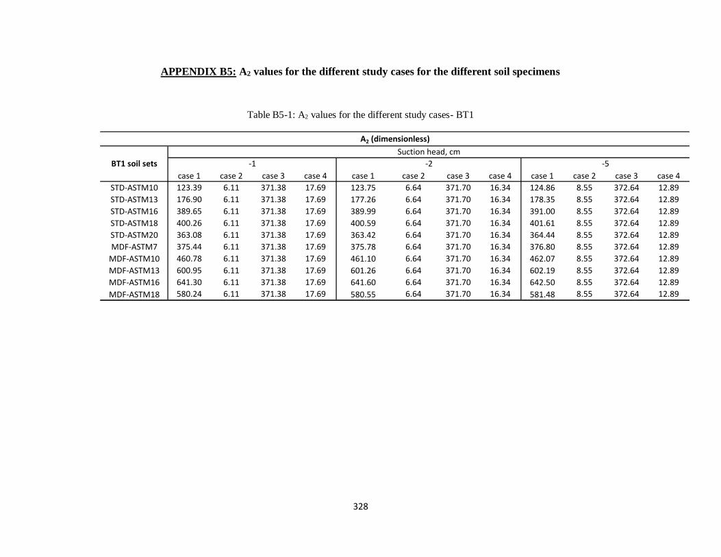
328

APPENDIX B5: A2 values for the different study cases for the different soil specimens

Table B5-1: A2 values for the different study cases- BT1

case 1 case 2 case 3 case 4 case 1 case 2 case 3 case 4 case 1 case 2 case 3 case 4

STD-ASTM10 123.39 6.11 371.38 17.69 123.75 6.64 371.70 16.34 124.86 8.55 372.64 12.89

STD-ASTM13 176.90 6.11 371.38 17.69 177.26 6.64 371.70 16.34 178.35 8.55 372.64 12.89

STD-ASTM16 389.65 6.11 371.38 17.69 389.99 6.64 371.70 16.34 391.00 8.55 372.64 12.89

STD-ASTM18 400.26 6.11 371.38 17.69 400.59 6.64 371.70 16.34 401.61 8.55 372.64 12.89

STD-ASTM20 363.08 6.11 371.38 17.69 363.42 6.64 371.70 16.34 364.44 8.55 372.64 12.89

MDF-ASTM7 375.44 6.11 371.38 17.69 375.78 6.64 371.70 16.34 376.80 8.55 372.64 12.89

MDF-ASTM10 460.78 6.11 371.38 17.69 461.10 6.64 371.70 16.34 462.07 8.55 372.64 12.89

MDF-ASTM13 600.95 6.11 371.38 17.69 601.26 6.64 371.70 16.34 602.19 8.55 372.64 12.89

MDF-ASTM16 641.30 6.11 371.38 17.69 641.60 6.64 371.70 16.34 642.50 8.55 372.64 12.89

MDF-ASTM18 580.24 6.11 371.38 17.69 580.55 6.64 371.70 16.34 581.48 8.55 372.64 12.89

A2 (dimensionless)

BT1 soil sets

Suction head, cm

-1 -2 -5

329

Appendix B5

Table B5-2: A2 values for the different study cases- BT2

case 1 case 2 case 3 case 1 case 2 case 3 case 1 case 2 case 3

STD-ASTM13 152.77 5.72 344.94 153.14 6.27 345.26 154.24 8.25 346.21

STD-ASTM16 231.39 5.72 344.94 231.75 6.27 345.26 232.82 8.25 346.21

STD-ASTM19.5 329.25 5.72 344.94 329.59 6.27 345.26 330.62 8.25 346.21

STD-ASTM22 368.85 5.72 344.94 369.19 6.27 345.26 370.21 8.25 346.21

MDF-ASTM8 356.19 5.72 344.94 356.52 6.27 345.26 357.52 8.25 346.21

MDF-ASTM11 182.25 5.72 344.94 182.62 6.27 345.26 183.72 8.25 346.21

MDF-ASTM13 330.24 5.72 344.94 330.58 6.27 345.26 331.60 8.25 346.21

MDF-ASTM15 243.30 5.72 344.94 243.66 6.27 345.26 244.73 8.25 346.21

MDF-ASTM16 148.85 5.72 344.94 149.22 6.27 345.26 150.32 8.25 346.21

A2 (Dimensionless)

BT2 soil sets

Suction head, cm

-1 -2 -5

330

Appendix B5

Table B5-2: A2 values for the different study cases- JF2


STD-ASTM10 163.66 6.11 371.38 17.69 164.03 6.64 371.70 16.34 165.12 8.55 372.64 12.89

STD-ASTM14 233.91 6.11 371.38 17.69 234.27 6.64 371.70 16.34 235.34 8.55 372.64 12.89

STD-ASTM16 144.23 6.11 371.38 17.69 143.73 6.64 371.70 16.34 142.21 8.55 372.64 12.89

STD-ASTM18 345.77 6.11 371.38 17.69 346.11 6.64 371.70 16.34 347.14 8.55 372.64 12.89

STD-ASTM21 492.53 6.11 371.38 17.69 492.85 6.64 371.70 16.34 493.82 8.55 372.64 12.89

MDF-ASTM8 204.95 6.11 371.38 17.69 205.31 6.64 371.70 16.34 206.40 8.55 372.64 12.89

MDF-ASTM11 222.58 6.11 371.38 17.69 222.94 6.64 371.70 16.34 224.02 8.55 372.64 12.89

MDF-ASTM13.5 161.97 6.11 371.38 17.69 162.33 6.64 371.70 16.34 163.42 8.55 372.64 12.89

MDF-ASTM15 159.73 6.11 371.38 17.69 160.09 6.64 371.70 16.34 161.18 8.55 372.64 12.89

MDF-ASTM17 334.22 6.11 371.38 17.69 334.22 6.64 371.70 16.34 335.25 8.55 372.64 12.89

A2 (Dimensionless)

JF2 soil sets

Suction head, cm

-1 -2 -5

331

APPENDIX B6: Derived Permeabilities for the different study cases for the different soil specimens

Table B6-1:Derived Permeabilities for the different study cases- BT1


STD-ASTM10 2.43E-08 4.91E-07 8.08E-09 1.70E-07 1.62E-08 3.01E-07 5.38E-09 1.22E-07 7.21E-09 1.05E-07 2.42E-09 6.98E-08





MDF-ASTM7 5.33E-09 3.27E-07 5.39E-09 1.13E-07 2.66E-09 1.51E-07 2.69E-09 6.12E-08 2.65E-09 1.17E-07 2.68E-09 7.76E-08





k (m/s)

BT1 soil sets

Suction head, cm

-1 -2 -5

BT1 soil sets


BT1 soil sets

standard Proctor energy h= -1cm

332

Table B6-2:Derived Permeabilities for the different study cases- BT2

case 1 case 2 case 3 case 1 case 2 case 3 case 1 case 2 case 3

STD-ASTM13 3.27E-08 8.74E-07 1.45E-08 1.96E-08 4.78E-07 8.69E-09 6.48E-09 1.21E-07 2.89E-09


STD-ASTM19.5 6.07E-09 3.50E-07 5.80E-09 3.03E-09 1.59E-07 2.90E-09 2.72E-09 1.09E-07 2.60E-09


MDF-ASTM8 1.12E-08 6.99E-07 1.16E-08 1.12E-08 6.38E-07 1.16E-08 1.12E-08 4.85E-07 1.16E-08





k (m/s)

-5

Suction head, cm

BT2 soil sets -1 -2

BT2 soil sets

standard Proctor energy h= -1cm BT2 soil sets


BT2 soil sets

standard Proctor energy h= -2cm BT2 soil sets


333

Table B6-3:Derived Permeabilities for the different study cases- JF2









MDF-ASTM13.5 1.85E-09 4.91E-08 8.08E-10 1.70E-08 1.23E-09 3.01E-08 5.38E-10 1.22E-08 1.22E-09 2.34E-08 5.37E-10 1.55E-08



k (m/s)

JF2 soil sets

Suction head, cm

-1 -2 -5

JF2 soil sets

standard Proctor energy h= -1cm

JF2 soil sets

JF2 soil sets


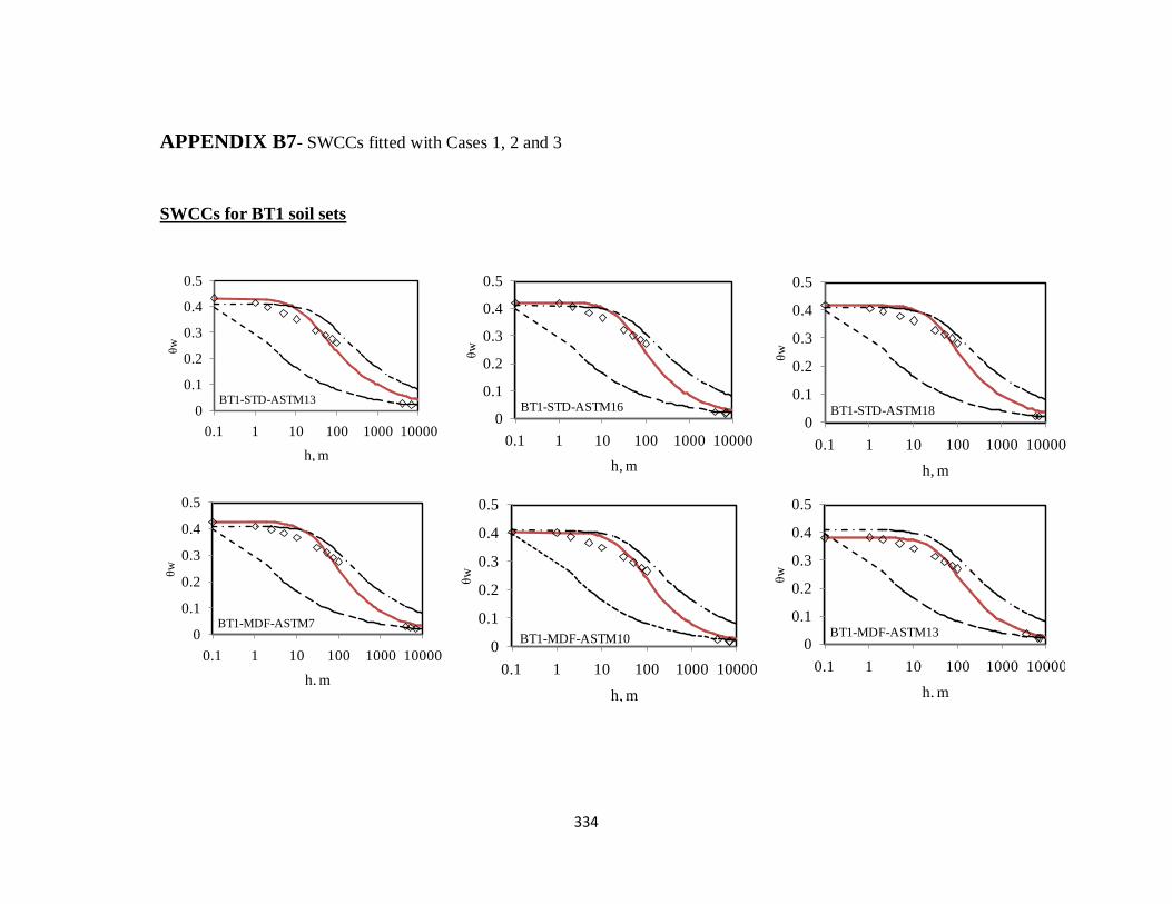
334

APPENDIX B7- SWCCs fitted with Cases 1, 2 and 3

SWCCs for BT1 soil sets

0

0.1

0.2

0.3

0.4

0.5

0.1 1 10 100 1000 10000

θw

h, m

BT1-STD-ASTM13

0

0.1

0.2

0.3

0.4

0.5

0.1 1 10 100 1000 10000

θw

h, m

BT1-STD-ASTM16

0

0.1

0.2

0.3

0.4

0.5

0.1 1 10 100 1000 10000

θw

h, m

BT1-STD-ASTM18

0

0.1

0.2

0.3

0.4

0.5

0.1 1 10 100 1000 10000

θw

h, m

BT1-MDF-ASTM7

0

0.1

0.2

0.3

0.4

0.5

0.1 1 10 100 1000 10000

θw

h, m

BT1-MDF-ASTM10 0

0.1

0.2

0.3

0.4

0.5

0.1 1 10 100 1000 10000

θw

h, m

BT1-MDF-ASTM13

335

SWCCs for BT2 soil sets

0

0.1

0.2

0.3

0.4

0.5

0.1 1 10 100 1000 10000

θw

h, m

BT1-MDF-ASTM16

0

0.1

0.2

0.3

0.4

0.5

0.1 1 10 100 1000 10000

θw

h, m

BT1-MDF-ASTM17.8

0

0.1

0.2

0.3

0.4

0.5

0.1 1 10 100100010000

θw

h, m

Data fitted using Case 1

Data Fitted using Case 2

Data fitted using Case 3

SWCC measured data

Legend:

BT1-STD-ASTM10

0

0.1

0.2

0.3

0.4

0.5

0.1 1 10 100 1000 10000

θw

h, m

BT2-STD-ASTM160

0.1

0.2

0.3

0.4

0.5

0.1 1 10 100 1000 10000

θw

h, m

BT2-STD-ASTM19.50

0.1

0.2

0.3

0.4

0.5

0.1 1 10 100 1000 10000

θw

h, m

BT2-MDF-ASTM8

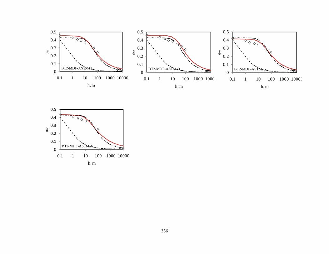
336

0

0.1

0.2

0.3

0.4

0.5

0.1 1 10 100 1000 10000

θw

h, m

BT2-MDF-ASTM11

0

0.1

0.2

0.3

0.4

0.5

0.1 1 10 100 1000 10000

θw

h, m

BT2-MDF-ASTM130

0.1

0.2

0.3

0.4

0.5

0.1 1 10 100 1000 10000

θw

h, m

BT2-MDF-ASTM15

0

0.1

0.2

0.3

0.4

0.5

0.1 1 10 100 1000 10000

θw

h, m

BT2-MDF-ASTM16

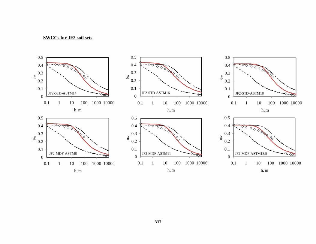
337

SWCCs for JF2 soil sets

0

0.1

0.2

0.3

0.4

0.5

0.1 1 10 100 1000 10000

θw

h, m

JF2-STD-ASTM140

0.1

0.2

0.3

0.4

0.5

0.1 1 10 100 1000 10000

θw

h, m

JF2-STD-ASTM160

0.1

0.2

0.3

0.4

0.5

0.1 1 10 100 1000 10000

θw

h, m

JF2-STD-ASTM18

0

0.1

0.2

0.3

0.4

0.5

0.1 1 10 100 1000 10000

θw

h, m

JF2-MDF-ASTM80

0.1

0.2

0.3

0.4

0.5

0.1 1 10 100 1000 10000

θw

h, m

JF2-MDF-ASTM110

0.1

0.2

0.3

0.4

0.5

0.1 1 10 100 1000 10000

θw

h, m

JF2-MDF-ASTM13.5

338

0

0.1

0.2

0.3

0.4

0.5

0.1 1 10 100 1000 10000

θw

h, m

JF2-MDF-ASTM15

0

0.1

0.2

0.3

0.4

0.5

0.1 1 10 100 1000 10000

θw

h, m

JF2-MDF-ASTM17

339

APPENDIX B7: V-G fitting parameters for the SWCC test data (Case 1)

BT1-soil sets n α Ѳs Ѳr SSE

STD-ASTM10 1.478 0.028 0.414 0.001 0.0049

STD-ASTM13 1.475 0.026 0.399 0.001 0.0051

STD-ASTM16 1.545 0.020 0.400 0.001 0.0037

STD-ASTM18 1.546 0.016 0.392 0.001 0.0031

STD-ASTM20 1.585 0.014 0.392 0.001 0.0063

MDF-ASTM7 1.545 0.018 0.398 0.001 0.0029

MDF-ASTM10 1.581 0.017 0.381 0.001 0.0031

MDF-ASTM13 1.566 0.015 0.368 0.001 0.0019

MDF-ASTM16 1.614 0.014 0.384 0.001 0.0029

MDF-ASTM18 1.595 0.014 0.377 0.001 0.0024

BT2-soil sets n α Ѳs Ѳr SSE

STD-ASTM13 1.443 0.036 0.413 0.001 0.0028

STD-ASTM16 1.514 0.025 0.396 0.001 0.0037

STD-ASTM19.5 1.555 0.019 0.403 0.001 0.0034

STD-ASTM22 1.576 0.017 0.399 0.001 0.0035

MDF-ASTM8 1.563 0.025 0.410 0.001 0.0014

MDF-ASTM11 1.543 0.027 0.416 0.001 0.0040

MDF-ASTM13 1.622 0.017 0.419 0.001 0.0044

MDF-ASTM15 1.536 0.022 0.379 0.001 0.0035

MDF-ASTM16 1.496 0.026 0.398 0.001 0.0043

JF2-soil sets n α Ѳs Ѳr SSE

STD-ASTM10 1.487 0.027 0.402 0.001 0.0044

STD-ASTM14 1.558 0.022 0.393 0.001 0.0062

STD-ASTM16 1.449 0.028 0.391 0.001 0.0056

STD-ASTM18 1.610 0.015 0.387 0.001 0.0053

STD-ASTM21 1.631 0.013 0.374 0.001 0.0043

MDF-ASTM8 1.499 0.026 0.400 0.000 0.0034

MDF-ASTM11 1.523 0.024 0.391 0.001 0.0048

MDF-ASTM13.5 1.478 0.024 0.372 0.001 0.0052

MDF-ASTM15 1.481 0.023 0.376 0.001 0.0056

MDF-ASTM17 1.627 0.014 0.361 0.001 0.0055

340

APPENDIX B8- Comparison of permeabilities from FWP and the different study cases using the mini-disk infiltrometer

BT1 soil sets

y = -4E-09x + 3E-08

y = -9E-08x + 5E-07

y = -1E-09x + 9E-09

y = -2E-08x + 2E-07

1E-12

1E-11

1E-10

1E-09

1E-08

1E-07

1E-06

0 1 2 3 4 5 6

k, m

/s

suction head, cm

BT1-STD-ASTM10

y = -4E-10x + 9E-09

y = -2E-08x + 3E-07

y = -2E-10x + 4E-09

y = 6E-10x + 8E-08

1E-12

1E-11

1E-10

1E-09

1E-08

1E-07

1E-06

0 1 2 3 4 5 6

k, m

/s

suction head, cm

BT1-STD-ASTM13

y = -6E-08x + 4E-07

y = -9E-10x + 7E-09

y = -2E-08x + 1E-07

1E-12

1E-11

1E-10

1E-09

1E-08

1E-07

1E-06

0 1 2 3 4 5 6

k, m

/s

suction head, cm

BT1-STD-ASTM16

y = -2E-08x + 1E-07

y = -3E-10x + 2E-09

y = -5E-09x + 4E-08

1E-12

1E-11

1E-10

1E-09

1E-08

1E-07

1E-06

0 1 2 3 4 5 6

k, m

/s

suction head, cm

BT1-STD-ASTM18

y = -9E-09x + 5E-08

y = -1E-10x + 9E-10

y = -2E-09x + 2E-08

1E-12

1E-11

1E-10

1E-09

1E-08

1E-07

1E-06

0 1 2 3 4 5 6

k, m

/s

suction head, cm

BT1-STD-ASTM20

y = -4E-08x + 3E-07

y = -5E-10x + 5E-09

y = -6E-09x + 1E-07

1E-12

1E-11

1E-10

1E-09

1E-08

1E-07

1E-06

0 1 2 3 4 5 6

k, m

/s

suction head, cm

BT1-MDF-ASTM7

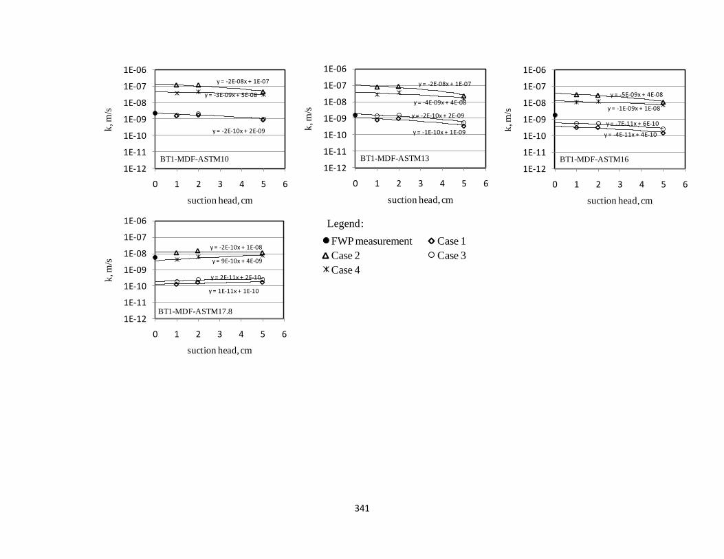
341

y = -2E-08x + 1E-07

y = -2E-10x + 2E-09

y = -3E-09x + 5E-08

1E-12

1E-11

1E-10

1E-09

1E-08

1E-07

1E-06

0 1 2 3 4 5 6

k, m

/s

suction head, cm

BT1-MDF-ASTM10

y = -1E-10x + 1E-09

y = -2E-08x + 1E-07

y = -2E-10x + 2E-09

y = -4E-09x + 4E-08

1E-12

1E-11

1E-10

1E-09

1E-08

1E-07

1E-06

0 1 2 3 4 5 6

k, m

/s

suction head, cm

BT1-MDF-ASTM13

y = -4E-11x + 4E-10

y = -5E-09x + 4E-08

y = -7E-11x + 6E-10

y = -1E-09x + 1E-08

1E-12

1E-11

1E-10

1E-09

1E-08

1E-07

1E-06

0 1 2 3 4 5 6

k, m

/s

suction head, cm

BT1-MDF-ASTM16

y = 1E-11x + 1E-10

y = -2E-10x + 1E-08

y = 2E-11x + 2E-10

y = 9E-10x + 4E-09

1E-12

1E-11

1E-10

1E-09

1E-08

1E-07

1E-06

0 1 2 3 4 5 6

k, m

/s

suction head, cm

BT1-MDF-ASTM17.8

y = -2E-08x + 1E-07

y = -2E-10x + 2E-09

y = -3E-09x + 5E-08

1E-12

1E-11

1E-10

1E-09

1E-08

1E-07

1E-06

0 1 2 3 4 5 6

k, m

/s

suction head, cm

FWP measurement Case 1

Case 2 Case 3

Case 4

BT1-MDF-ASTM10

Legend:

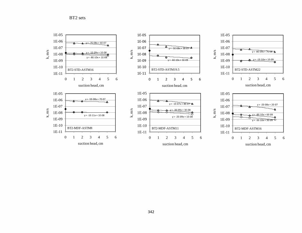
342

y = -1E-09x + 1E-08

y = -7E-08x + 6E-07

y = -8E-10x + 1E-08

1E-11

1E-10

1E-09

1E-08

1E-07

1E-06

1E-05

0 1 2 3 4 5 6

k, m

/s

suction head, cm

BT2-STD-ASTM16

y = -5E-08x + 3E-07

y = -6E-10x + 5E-09

1E-11

1E-10

1E-09

1E-08

1E-07

1E-06

1E-05

0 1 2 3 4 5 6

k, m

/s

suction head, cm

BT2-STD-ASTM19.5

y = -8E-09x + 7E-08

y = -1E-10x + 1E-09

1E-11

1E-10

1E-09

1E-08

1E-07

1E-06

1E-05

0 1 2 3 4 5 6

k, m

/s

suction head, cm

BT2-STD-ASTM22

y = -5E-08x + 7E-07

y = -1E-11x + 1E-08

1E-11

1E-10

1E-09

1E-08

1E-07

1E-06

1E-05

0 1 2 3 4 5 6

k, m

/s

suction head, cm

BT2-MDF-ASTM8

y = -3E-09x + 3E-08

y = -1E-07x + 8E-07

y = -2E-09x + 1E-08

1E-11

1E-10

1E-09

1E-08

1E-07

1E-06

1E-05

0 1 2 3 4 5 6

k, m

/s

suction head, cm

BT2-MDF-ASTM11

y = -8E-10x + 6E-09

y = -2E-08x + 2E-07

y = -3E-10x + 3E-09

1E-11

1E-10

1E-09

1E-08

1E-07

1E-06

1E-05

0 1 2 3 4 5 6

k, m

/s

suction head, cm

BT2-MDF-ASTM16

BT2 sets

343

y = -3E-10x + 5E-09

y = -1E-08x + 1E-07

y = -1E-10x + 3E-09

y = 1E-09x + 4E-08

1E-12

1E-11

1E-10

1E-09

1E-08

1E-07

1E-06

0 1 2 3 4 5 6

k, m

/s

suction head, cm

JF2-STD-ASTM16

y = -4E-10x + 9E-09

y = 5E-12x + 1E-10

y = 4E-10x + 3E-09

1E-12

1E-11

1E-10

1E-09

1E-08

1E-07

1E-06

0 1 2 3 4 5 6

k, m

/s

suction head, cm

JF2-STD-ASTM18

y = 4E-12x + 2E-11

y = 8E-11x + 2E-09

y = 5E-12x + 3E-11

y = 2E-10x + 5E-10

1E-12

1E-11

1E-10

1E-09

1E-08

1E-07

1E-06

0 1 2 3 4 5 6

k, m

/s

suction head, cm

JF2-STD-ASTM21

y = -1E-10x + 2E-09

y = -5E-09x + 5E-08

y = -5E-11x + 8E-10

y = -3E-11x + 1E-08

1E-12

1E-11

1E-10

1E-09

1E-08

1E-07

1E-06

0 1 2 3 4 5 6

k, m

/s

suction head, cm

JF2-MDF-ASTM13.5

y = 5E-11x + 4E-10

y = 1E-10x + 1E-08

y = 2E-11x + 2E-10

y = 1E-09x + 3E-09

1E-12

1E-11

1E-10

1E-09

1E-08

1E-07

1E-06

0 1 2 3 4 5 6

k, m

/s

suction head, cm

JF2-MDF-ASTM15

y = -3E-10x + 5E-09

y = -7E-14x + 8E-11

y = 2E-10x + 2E-09

1E-12

1E-11

1E-10

1E-09

1E-08

1E-07

1E-06

0 1 2 3 4 5 6

k, m

/s

suction head, cm

JF2-MDF-ASTM17

JF2 soil sets

344

y = -4E-10x + 5E-09

y = -2E-08x + 2E-07

y = -2E-10x + 3E-09

y = -1E-09x + 6E-08

1E-12

1E-11

1E-10

1E-09

1E-08

1E-07

1E-06

0 1 2 3 4 5 6

k, m

/s

suction head, cm

JF2-MDF-ASTM11

345

Appendix C- UC and BTS

data

Contains Appendices C1-C4 (Referenced to in Chapter 6)

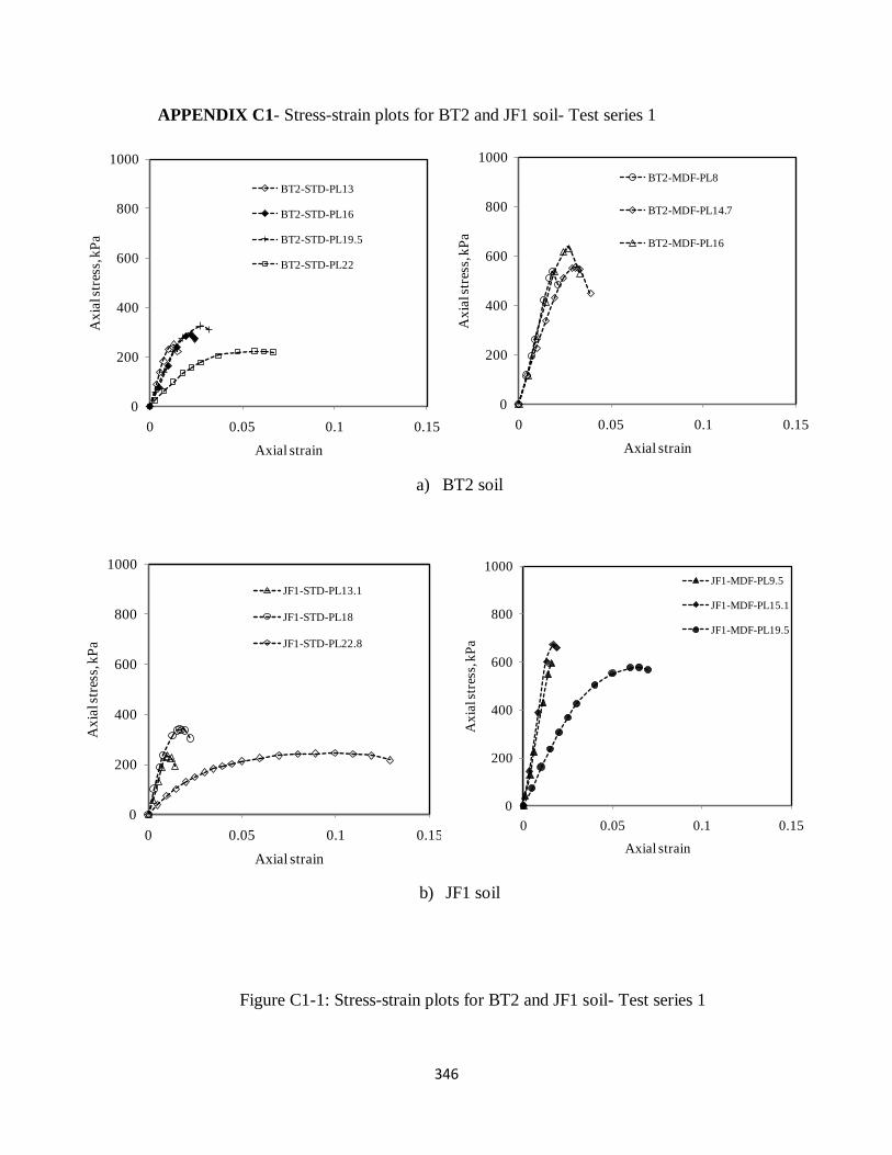
346

APPENDIX C1- Stress-strain plots for BT2 and JF1 soil- Test series 1

a) BT2 soil

b) JF1 soil

Figure C1-1: Stress-strain plots for BT2 and JF1 soil- Test series 1

0

200

400

600

800

1000

0 0.05 0.1 0.15

Ax

ial s

tres

s, k

Pa

Axial strain

BT2-STD-PL13

BT2-STD-PL16

BT2-STD-PL19.5

BT2-STD-PL22

0

200

400

600

800

1000

0 0.05 0.1 0.15

Ax

ial s

tres

s, k

Pa

Axial strain

BT2-MDF-PL8

BT2-MDF-PL14.7

BT2-MDF-PL16

0

200

400

600

800

1000

0 0.05 0.1 0.15

Ax

ial s

tres

s, k

Pa

Axial strain

JF1-STD-PL13.1

JF1-STD-PL18

JF1-STD-PL22.8

0

200

400

600

800

1000

0 0.05 0.1 0.15

Ax

ial s

tres

s, k

Pa

Axial strain

JF1-MDF-PL9.5

JF1-MDF-PL15.1

JF1-MDF-PL19.5

347

APPENDIX C2- Stress-strain plots for BT2 and JF1 soil (effect of compaction energy)-

Test series 1

a) BT2

b) JF1

Figure C2-1: Stress-strain plots from UCS test for both standard and modified Proctor

compacted soils for BT2 and JF1 (Test series 1)

0

200

400

600

800

1000

0 0.05 0.1 0.15

Ax

ial s

tres

s, k

Pa

Axial strain

BT2-STD-PL13

BT2-STD-PL16

BT2-STD-PL19.5

BT2-STD-PL22

BT2-MDF-PL8

BT2-MDF-PL15

BT2-MDF-PL16

0

200

400

600

800

1000

0 0.05 0.1 0.15

Ax

ial s

tres

s, k

Pa

Axial strain

JF1-STD-PL13

JF1-STD-PL18

JF1-STD-PL22

JF1-MDF-PL9

JF1-MDF-PL15

JF1-MDF-PL19.5

348

APPENDIX C3- Stress-strain plots sample sets D to I- Test series 2

Sample set D

Sample set E

Sample set F

0

500

1000

1500

0 0.02 0.04 0.06 0.08 0.1

Ax

ial s

tres

s, k

Pa

Axial strain

20.2

20.2

20.2

18.4

17

16.5

16

15.2

15

decreasing

water content

w%

0

500

1000

1500

0 0.02 0.04 0.06 0.08 0.1

Ax

ial s

tres

s, k

Pa

Axial strain

14.2

12.6

12

9.3

8.3

8

7.5

5.8

w%

0

500

1000

1500

0 0.02 0.04 0.06 0.08 0.1

Ax

ial s

tres

s, k

Pa

Axial strain

16

16.1

16.1

14.3

13.1

12.2

9.1

decreasing

water content

w%

0

500

1000

1500

0 0.02 0.04 0.06 0.08 0.1

Ax

ial s

tres

s, k

Pa

Axial strain

7.5

6

1.4

1.4

1.4

w%

0

500

1000

1500

0 0.02 0.04 0.06 0.08 0.1

Ax

ial s

tres

s, k

Pa

Axial strain

22.2

22.3

22.2

19.8

19.1

18.3

16.1

14

12.2

decreasing

water content

w%

0

500

1000

1500

0 0.02 0.04 0.06 0.08 0.1

Ax

ial s

tres

s, k

Pa

Axial strain

11.7

11.2

9.7

1.4

1.2

w%

349

Sample set G

Sample set H

Sample set I

0

500

1000

1500

0 0.02 0.04 0.06 0.08 0.1

Ax

ial s

tres

s, k

Pa

Axial strain

17

17

17

15.3

15.2

14.8

14.7

13.7

13.4

decreasing

water content

w%

0

500

1000

1500

0 0.02 0.04 0.06 0.08 0.1

Ax

ial s

tres

s, k

Pa

Axial strain

11

10

9.3

9

8

7.8

7.5

6.2

w%

0

500

1000

1500

0 0.02 0.04 0.06 0.08 0.1

Ax

ial s

tres

s, k

Pa

Axial strain

18

17.6

17.6

17.5

16.2

15.8

15.4

15

14.6

14.2

decreasing

water content

w%

0

500

1000

1500

0 0.02 0.04 0.06 0.08 0.1

Ax

ial s

tres

s, k

Pa

Axial strain

13.2

13.2

13

11.7

11.4

11.1

10.7

9.8

8.5

w%

0

500

1000

1500

0 0.02 0.04 0.06 0.08 0.1

Ax

ial s

tres

s, k

Pa

Axial strain

20

20

19.5

9.2

17.4

16.8

16.3

15

15

decreasing

water content

w%

0

500

1000

1500

0 0.02 0.04 0.06 0.08 0.1

Ax

ial s

tres

s, k

Pa

Axial strain

12.5

11

11

10.4

9.4

9.3

7.7

7.1

6.1

w%

350

APPENDIX C4- Variation of UCS and BTS with degree of saturation and SWCC for sample sets D to I

– Test series 2

a) Sample set D

b) Sample set E

c) Sample set F

1

10

100

1000

10000

100000

1000000

0 0.2 0.4 0.6 0.8 1

Matr

ic s

uct

ion o

r st

ren

gth

, kP

a


SWCC

UCS

BTS

S = 80% 95%

0

0.2

0.4

0.6

0.8

1

0 0.1 0.2 0.3

Vo

id r

ati

o


SWCC samples

UCS samples

BTS samples

S = 80% 95%

1

10

100

1000

10000

100000

1000000

0 0.2 0.4 0.6 0.8 1

Matr

ic s

uct

ion o

r st

ren

gth

, kP

a


SWCC

UCS

BTS

S = 80% 95%

0

0.2

0.4

0.6

0.8

1

0 0.1 0.2 0.3

Vo

id r

ati

o


SWCC samples

UCS samples

BTS samples

S = 80% 95%

351

d) Sample G

e) Sample H

f) Sample I

1

10

100

1000

10000

100000

1000000

0 0.2 0.4 0.6 0.8 1

Matr

ic s

uct

ion o

r st

ren

gth

, kP

a


SWCCUCSBTS

S = 82% 97%

0

0.2

0.4

0.6

0.8

1

0 0.1 0.2 0.3

Vo

id r

ati

o


SWCC samples

UCS samples

BTS samples

S = 82% 97%

1

10

100

1000

10000

100000

1000000

0 0.2 0.4 0.6 0.8 1

Matr

ic s

uct

ion o

r st

ren

gth

, kP

a


SWCC

UCS

BTS

S = 82% 97%

0

0.2

0.4

0.6

0.8

1

0 0.1 0.2 0.3

Vo

id r

ati

o


SWCC samples

UCS samples

BTS samples

S = 82% 97%

1

10

100

1000

10000

100000

1000000

0 0.2 0.4 0.6 0.8 1

Matr

ic s

uct

ion o

r st

ren

gth

, kP

a


UCS

BTS

SWCC

S = 82% 97%

0

0.2

0.4

0.6

0.8

1

0 0.1 0.2 0.3

Vo

id r

ati

o


SWCC samples

UCS samples

BTS samples

S = 82% 97%

352

Appendix D-UC and UU data

Contains Appendices D1-D6 (Referenced to in Chapter 7)

353

APPENDIX D1- UCS and UU stress-strain plots

Legend

Figure D1-1: UC and UU stress-strain plots for BT1 soil specimens

0

500

1000

1500

2000

0 0.1 0.2 0.3

Dev

iato

r st

ress

, kP

a

Axial strain

BT1-MDF-PL7

0

500

1000

1500

2000

0 0.1 0.2 0.3

Dev

iato

r st

ress

, kP

a

Axial strain

BT1-MDF-PL13

0

500

1000

1500

2000

0 0.1 0.2 0.3

Dev

iato

r st

ress

, kP

a

Axial strain

BT1-MDF-PL10

0

500

1000

1500

2000

0 0.1 0.2 0.3

Dev

iato

r st

ress

, kP

a

Axial strain

BT1-MDF-PL16

0

500

1000

1500

2000

0 0.1 0.2 0.3

Dev

iato

r st

ress

, kP

a

Axial strain

BT1-MDF-PL18

0

500

1000

1500

2000

0 0.1 0.2 0.3

Dev

iato

r st

ress

, kP

a

Axial strain

600

300

150

70

0

σ3-ua , kPa

354

Figure D1-2: UC and UU stress-strain plots for BT2 soil specimens

0

500

1000

1500

2000

0 0.1 0.2 0.3

Dev

iato

r st

ress

, kP

a

Axial strain

BT2-STD-PL12

0

500

1000

1500

2000

0 0.1 0.2 0.3

Dev

iato

r st

ress

, kP

a

Axial strain

BT2-STD-PL19.5

0

500

1000

1500

2000

0 0.1 0.2 0.3

Dev

iato

r st

ress

, kP

a

Axial strain

BT2-STD-PL16

0

500

1000

1500

2000

0 0.1 0.2 0.3

Dev

iato

r st

ress

, kP

a

Axial strain

BT2-STD-PL22

0

500

1000

1500

2000

0 0.1 0.2 0.3

Dev

iato

r st

ress

, kP

a

Axial strain

BT2-MDF-PL8

0

500

1000

1500

2000

0 0.1 0.2 0.3

Dev

iato

r st

ress

, kP

a

Axial strain

BT2-MDF-PL16

355

Figure D1-3: UC and UU stress-strain plots for JF1 soil specimens

0

500

1000

1500

2000

0 0.1 0.2 0.3

Dev

iato

r st

ress

, kP

a

Axial strain

JF1-STD-PL13

0

500

1000

1500

2000

0 0.1 0.2 0.3

Dev

iato

r st

ress

, kP

a

Axial strain

JF1-STD-PL22

0

500

1000

1500

2000

0 0.1 0.2 0.3

Dev

iato

r st

ress

, kP

a

Axial strain

JF1-STD-PL18

0

500

1000

1500

2000

0 0.1 0.2 0.3

Dev

iato

r st

ress

, kP

a

Axial strain

JF1-MDF-PL19.5

0

500

1000

1500

2000

0 0.1 0.2 0.3

Dev

iato

r st

ress

, kP

a

Axial strain

JF1-MDF-PL9.5

0

500

1000

1500

2000

0 0.1 0.2 0.3

Dev

iato

r st

ress

, kP

a

Axial strain

JF1-MDF-PL15

356


0

500

1000

1500

2000

0 0.1 0.2 0.3

Dev

iato

r st

ress

, kP

a

Axial strain

JF2-STD-PL10

0

500

1000

1500

2000

0 0.1 0.2 0.3

Dev

iato

r st

ress

, kP

a

Axial strain

JF2-STD-PL18

0

500

1000

1500

2000

0 0.1 0.2 0.3

Dev

iato

r st

ress

, kP

a

Axial strain

JF2-STD-PL14

0

500

1000

1500

2000

0 0.1 0.2 0.3

Dev

iato

r st

ress

, kP

a

Axial strain

JF2-STD-PL21

0

500

1000

1500

2000

0 0.1 0.2 0.3

Dev

iato

r st

ress

, kP

a

Axial strain

JF2-STD-PL16

0

500

1000

1500

2000

0 0.1 0.2 0.3

Dev

iato

r st

ress

, kP

a

Axial strain

JF2-MDF-PL17

357


0

500

1000

1500

2000

0 0.1 0.2 0.3

Dev

iato

r st

ress

, kP

a

Axial strain

JF2-MDF-PL8

0

500

1000

1500

2000

0 0.1 0.2 0.3

Dev

iato

r st

ress

, kP

a

Axial strain

JF2-MDF-PL15

0

500

1000

1500

2000

0 0.1 0.2 0.3

Dev

iato

r st

ress

, kP

a

Axial strain

JF2-MDF-PL11

0

500

1000

1500

2000

0 0.1 0.2 0.3

Dev

iato

r st

ress

, kP

a

Axial strain

JF2-MDF-PL17

358

Appendix D2: Effect of confining pressure on the stress-strain behavior

Figure D2-1: Effect of net confining pressure on the stress-strain plots of BT1 soil specimens

compacted at modified Proctor

0

500

1000

1500

2000

0 0.1 0.2 0.3

Dev

iato

r s

tres

s, k

Pa

Axial strain

BT1-MDF-PL7

BT1-MDF-PL10

BT1-MDF-PL13

BT1-MDF-PL16

BT1-MDF-PL17.8

σ-ua=70 kPa

0

500

1000

1500

2000

0 0.1 0.2 0.3

Dev

iato

r s

tres

s, k

Pa

Axial strain

BT1-MDF-PL7

BT1-MDF-PL10

BT1-MDF-PL13

BT1-MDF-PL16

BT1-MDF-PL17.8

σ-ua= 150 kPa

0

500

1000

1500

2000

0 0.1 0.2 0.3

Dev

iato

r s

tres

s, k

Pa

Axial strain

BT1-MDF-PL7

BT1-MDF-PL10

BT1-MDF-PL13

BT1-MDF-PL16

BT1-MDF-PL17.8

σ-ua=300kPa

0

500

1000

1500

2000

0 0.1 0.2 0.3

Dev

iato

r s

tres

s, k

Pa

Axial strain

BT1-MDF-PL7

BT1-MDF-PL10

BT1-MDF-PL13

BT1-MDF-PL16

BT1-MDF-PL17.8

σ-ua=600kPa

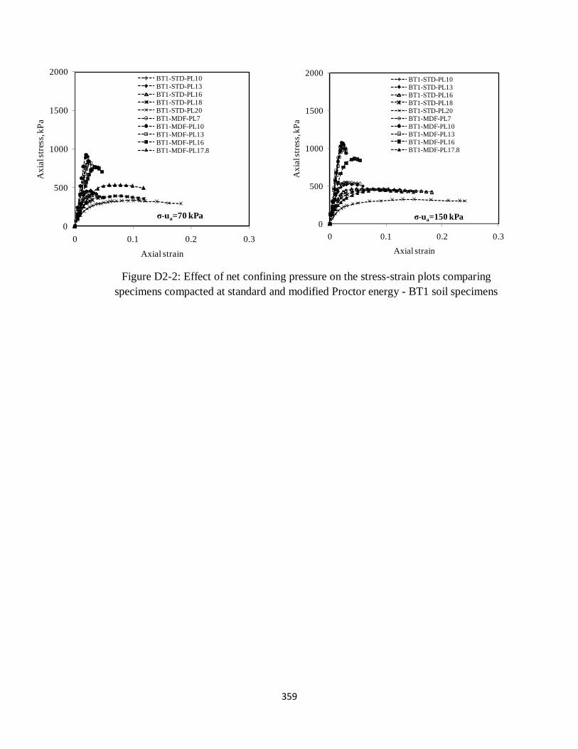
359

Figure D2-2: Effect of net confining pressure on the stress-strain plots comparing

specimens compacted at standard and modified Proctor energy - BT1 soil specimens

0

500

1000

1500

2000

0 0.1 0.2 0.3

Ax

ial s

tres

s, k

Pa

Axial strain

BT1-STD-PL10

BT1-STD-PL13

BT1-STD-PL16

BT1-STD-PL18

BT1-STD-PL20

BT1-MDF-PL7

BT1-MDF-PL10

BT1-MDF-PL13

BT1-MDF-PL16

BT1-MDF-PL17.8

σ-ua=70 kPa0

500

1000

1500

2000

0 0.1 0.2 0.3

Ax

ial s

tres

s, k

Pa

Axial strain

BT1-STD-PL10

BT1-STD-PL13

BT1-STD-PL16

BT1-STD-PL18

BT1-STD-PL20

BT1-MDF-PL7

BT1-MDF-PL10

BT1-MDF-PL13

BT1-MDF-PL16

BT1-MDF-PL17.8

σ-ua=150 kPa

360

Figure D2-3: Effect of net confining pressure on the stress-strain plots of BT2 soil specimens compacted

at standard Proctor

0

500

1000

1500

2000

0 0.1 0.2 0.3

Ax

ial s

tres

s, k

Pa

Axial strain

BT2-STD-PL13

BT2-STD-PL16

BT2-STD-PL19.5

BT2-STD-PL22

σ-ua=70 kPa0

500

1000

1500

2000

0 0.1 0.2 0.3

Ax

ial s

tres

s, k

Pa

Axial strain

BT2-STD-PL13

BT2-STD-PL16

BT2-STD-PL19.5

BT2-STD-PL22

σ-ua=150 kPa

0

500

1000

1500

2000

0 0.1 0.2 0.3

Ax

ial s

tres

s, k

Pa

Axial strain

BT2-STD-PL13

BT2-STD-PL16

BT2-STD-PL19.5

BT2-STD-PL22

σ-ua=300 kPa 0

500

1000

1500

2000

0 0.1 0.2 0.3

Ax

ial s

tres

s, k

Pa

Axial strain

BT2-STD-PL13

BT2-STD-PL16

BT2-STD-PL19.5

BT2-STD-PL22

σ-ua=600 kPa

361

Figure D2-4: Effect of net confining pressure on the stress-strain plots of BT2 soil specimens compacted

at modified Proctor

0

500

1000

1500

2000

0 0.1 0.2 0.3

Ax

ial s

tres

s, k

Pa

Axial strain

BT2-MDF-PL15

BT2-MDF-PL16

σ-ua=70 kPa

0

500

1000

1500

2000

0 0.1 0.2 0.3

Ax

ial s

tres

s, k

Pa

Axial strain

BT2-MDF-PL8

BT2-MDF-PL15

BT2-MDF-PL16

σ-ua=150 kPa

0

500

1000

1500

2000

0 0.1 0.2 0.3

Ax

ial s

tres

s, k

Pa

Axial strain

BT2-MDF-PL8

BT2-MDF-PL15

BT2-MDF-PL16

σ-ua=300 kPa0

500

1000

1500

2000

0 0.1 0.2 0.3

Ax

ial s

tres

s, k

Pa

Axial strain

BT2-MDF-PL8

BT2-MDF-PL15

BT2-MDF-PL16

σ-ua=600 kPa

362

Figure D2-5: Effect of net confining pressure on the stress-strain plots comparing specimens

compacted at standard and modified Proctor energy – BT2 soil specimens

0

500

1000

1500

2000

0 0.1 0.2 0.3

Ax

ial s

tres

s, k

Pa

Axial strain

BT2-STD-PL13

BT2-STD-PL16

BT2-STD-PL19.5

BT2-STD-PL22

BT2-MDF-PL15

BT2-MDF-PL16

σ-ua=70 kPa0

500

1000

1500

2000

0 0.1 0.2 0.3

Ax

ial s

tres

s, k

Pa

Axial strain

BT2-STD-PL13

BT2-STD-PL16

BT2-STD-PL19.5

BT2-STD-PL22

BT2-MDF-PL8

BT2-MDF-PL15

BT2-MDF-PL16

σ-ua=150 kPa

0

500

1000

1500

2000

0 0.1 0.2 0.3

Ax

ial s

tres

s, k

Pa

Axial strain

BT2-STD-PL13

BT2-STD-PL16

BT2-STD-PL19.5

BT2-STD-PL22

BT2-MDF-PL8

BT2-MDF-PL15

BT2-MDF-PL16

σ-ua=300 kPa0

500

1000

1500

2000

0 0.1 0.2 0.3

Ax

ial s

tres

s, k

Pa

Axial strain

BT2-STD-PL13

BT2-STD-PL16

BT2-STD-PL19.5

BT2-STD-PL22

BT2-MDF-PL8

BT2-MDF-PL15

BT2-MDF-PL16

σ-ua=600 kPa

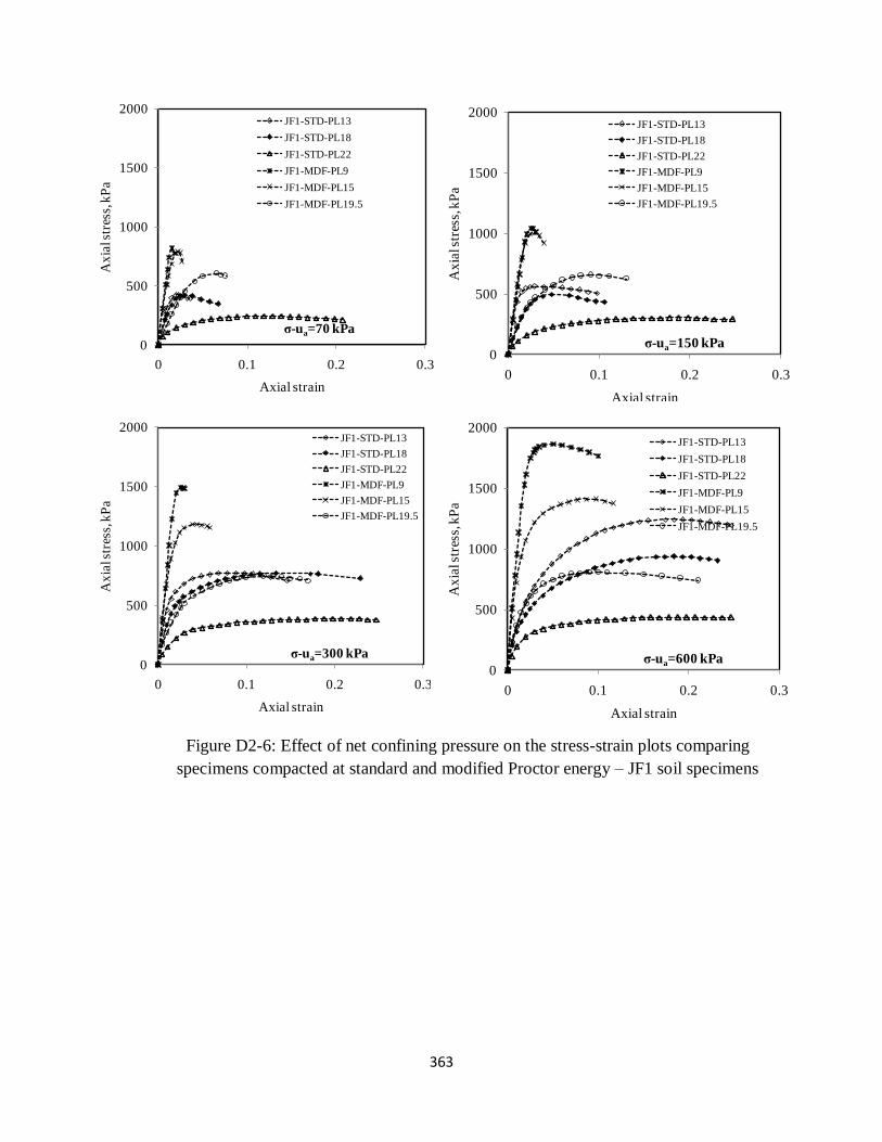
363

Figure D2-6: Effect of net confining pressure on the stress-strain plots comparing

specimens compacted at standard and modified Proctor energy – JF1 soil specimens

0

500

1000

1500

2000

0 0.1 0.2 0.3

Ax

ial s

tres

s, k

Pa

Axial strain

JF1-STD-PL13

JF1-STD-PL18

JF1-STD-PL22

JF1-MDF-PL9

JF1-MDF-PL15

JF1-MDF-PL19.5

σ-ua=70 kPa

0

500

1000

1500

2000

0 0.1 0.2 0.3

Ax

ial s

tres

s, k

Pa

Axial strain

JF1-STD-PL13

JF1-STD-PL18

JF1-STD-PL22

JF1-MDF-PL9

JF1-MDF-PL15

JF1-MDF-PL19.5

σ-ua=150 kPa

0

500

1000

1500

2000

0 0.1 0.2 0.3

Ax

ial s

tres

s, k

Pa

Axial strain

JF1-STD-PL13

JF1-STD-PL18

JF1-STD-PL22

JF1-MDF-PL9

JF1-MDF-PL15

JF1-MDF-PL19.5

σ-ua=300 kPa

0

500

1000

1500

2000

0 0.1 0.2 0.3

Ax

ial s

tres

s, k

Pa

Axial strain

JF1-STD-PL13

JF1-STD-PL18

JF1-STD-PL22

JF1-MDF-PL9

JF1-MDF-PL15

JF1-MDF-PL19.5

σ-ua=600 kPa

364

Figure D2-7: Effect of net confining pressure on the stress-strain plots of JF2 soil specimens

compacted at standard Proctor

0

500

1000

1500

2000

0 0.1 0.2 0.3

Dev

iato

r s

tres

s, k

Pa

Axial strain

JF2-STD-PL10

JF2-STD-PL14

JF2-STD-PL16

JF2-STD-PL18

JF2-STD-PL20

σ-ua = 70 kPa

0

500

1000

1500

2000

0 0.1 0.2 0.3

Dev

iato

r s

tres

s, k

Pa

Axial strain

JF2-STD-PL10

JF2-STD-PL14

JF2-STD-PL16

JF2-STD-PL18

JF2-STD-PL20

σ-ua = 150 kPa

0

500

1000

1500

2000

0 0.1 0.2 0.3

Dev

iato

r s

tres

s, k

Pa

Axial strain

JF2-STD-PL10

JF2-STD-PL14

JF2-STD-PL16

JF2-STD-PL18

JF2-STD-PL20

σ-ua = 300 kPa0

500

1000

1500

2000

0 0.1 0.2 0.3

Dev

iato

r s

tres

s, k

Pa

Axial strain

JF2-STD-PL10

JF2-STD-PL14

JF2-STD-PL16

JF2-STD-PL18

JF2-STD-PL20

σ-ua = 600 kPa

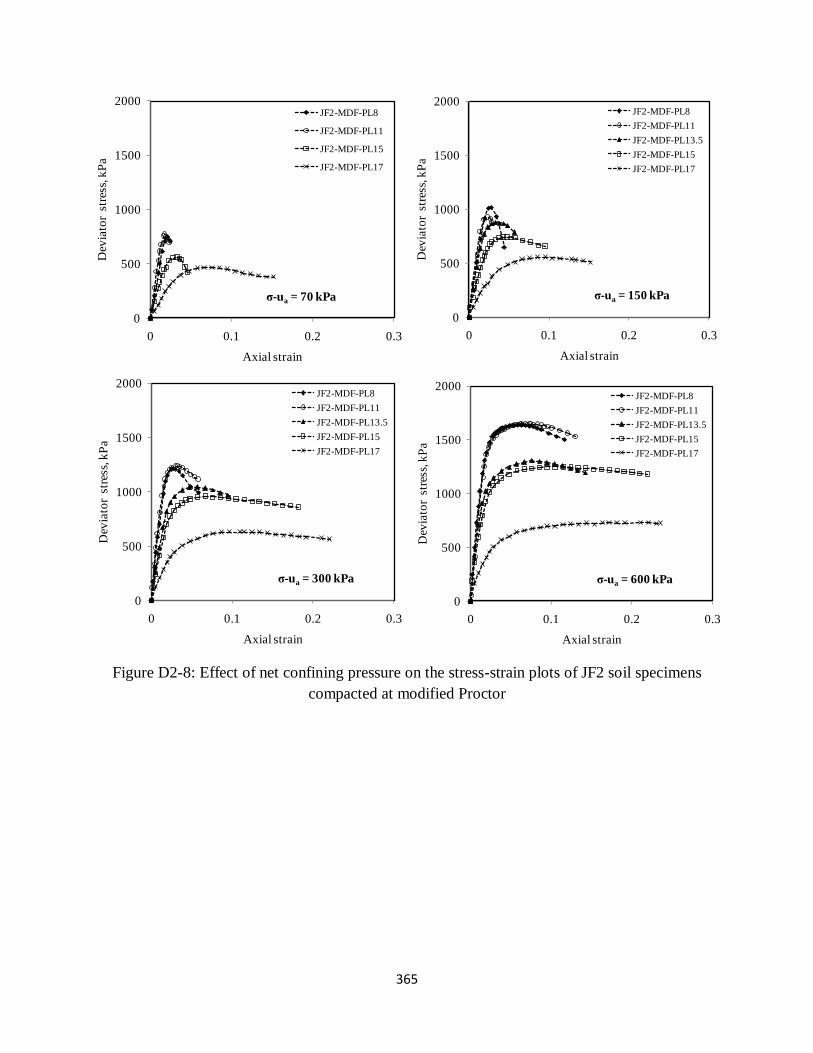
365

Figure D2-8: Effect of net confining pressure on the stress-strain plots of JF2 soil specimens

compacted at modified Proctor

0

500

1000

1500

2000

0 0.1 0.2 0.3

Dev

iato

r s

tres

s, k

Pa

Axial strain

JF2-MDF-PL8

JF2-MDF-PL11

JF2-MDF-PL15

JF2-MDF-PL17

σ-ua = 70 kPa

0

500

1000

1500

2000

0 0.1 0.2 0.3

Dev

iato

r s

tres

s, k

Pa

Axial strain

JF2-MDF-PL8

JF2-MDF-PL11

JF2-MDF-PL13.5

JF2-MDF-PL15

JF2-MDF-PL17

σ-ua = 150 kPa

0

500

1000

1500

2000

0 0.1 0.2 0.3

Dev

iato

r s

tres

s, k

Pa

Axial strain

JF2-MDF-PL8

JF2-MDF-PL11

JF2-MDF-PL13.5

JF2-MDF-PL15

JF2-MDF-PL17

σ-ua = 300 kPa

0

500

1000

1500

2000

0 0.1 0.2 0.3

Dev

iato

r s

tres

s, k

Pa

Axial strain

JF2-MDF-PL8

JF2-MDF-PL11

JF2-MDF-PL13.5

JF2-MDF-PL15

JF2-MDF-PL17

σ-ua = 600 kPa

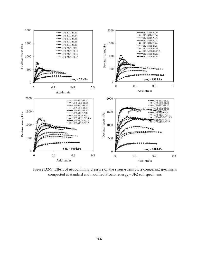
366

Figure D2-9: Effect of net confining pressure on the stress-strain plots comparing specimens

compacted at standard and modified Proctor energy – JF2 soil specimens

0

500

1000

1500

2000

0 0.1 0.2 0.3

Dev

iato

r s

tres

s, k

Pa

Axial strain

JF2-STD-PL10

JF2-STD-PL14

JF2-STD-PL16

JF2-STD-PL18

JF2-STD-PL20

JF2-MDF-PL8

JF2-MDF-PL11

JF2-MDF-PL15

JF2-MDF-PL17

σ-ua = 70 kPa0

500

1000

1500

2000

0 0.1 0.2 0.3

Dev

iato

r s

tres

s, k

Pa

Axial strain

JF2-STD-PL10

JF2-STD-PL14

JF2-STD-PL16

JF2-STD-PL18

JF2-STD-PL20

JF2-MDF-PL8

JF2-MDF-PL11

JF2-MDF-PL13.5

JF2-MDF-PL15

JF2-MDF-PL17

σ-ua = 150 kPa

0

500

1000

1500

2000

0 0.1 0.2 0.3

Dev

iato

r s

tres

s, k

Pa

Axial strain

JF2-STD-PL10JF2-STD-PL14JF2-STD-PL16JF2-STD-PL18JF2-STD-PL20JF2-MDF-PL8JF2-MDF-PL11JF2-MDF-PL13.5JF2-MDF-PL15JF2-MDF-PL17

σ-ua = 300 kPa0

500

1000

1500

2000

0 0.1 0.2 0.3

Dev

iato

r s

tres

s, k

Pa

Axial strain

JF2-STD-PL10JF2-STD-PL14JF2-STD-PL16JF2-STD-PL18JF2-STD-PL20JF2-MDF-PL8JF2-MDF-PL11JF2-MDF-PL13.5JF2-MDF-PL15JF2-MDF-PL17

σ-ua = 600 kPa

367

Appendix D3- Variation of qu with net confining pressure, compaction water content and

compaction effort

a) BT2 soil

b) JF1 soil

Figure D3-1:Variation of qu with net confining pressure, compaction water content and

compaction effort for BT2 and JF1

0

500

1000

1500

2000

5 10 15 20 25

qu, k

Pa


0 (UCS)

70

150

300

600

σ3-ua (kPa)

BT2-Standard Proctor energy

0

500

1000

1500

2000

5 10 15 20 25

qu, k

Pa


0 (UCS)

150

300

600

σ3-ua (kPa)


0

500

1000

1500

2000

5 10 15 20 25

qu, k

Pa


0 (UCS)

70

150

300

600

σ3-ua (kPa)

JF1-Standard Proctor energy0

500

1000

1500

2000

5 10 15 20 25

qu, k

Pa


0 (UCS)

150

300

600

σ3-ua (kPa)


368

Appendix D4- CU Multi-stage test- summary of results

Table D4-1: Saturated shear strength parameters for BT1

Sample id stage σ3f, kPa (σ1- σ3)f,

kPa

uf, kPa εf, % ϕ’o c’, kPa

BT1-STD-PL10

1 320 76.5 283.7

20.0 29.0 3 2 390 141.8 312.6

3 540 400.0 339.4

BT1-STD-PL13

1 270 78.7 237.2

12.5 30.6 1 2 340 157.1 255.2

3 490 332.5 330.3

BT1-STD-PL16

1 320 73.0 281.6

19.6 28.0 3 2 390 143.7 313.5

3 540 307.5 371.4

BT1-STD-PL18

1 370 82.5 327.1

12.0 27.5 4 2 440 160.3 355.1

3 590 312.8 415.6

BT2-STD-PL20

1 320 99.6 265.4

18.5 27.5 3 2 390 178.6 291.6

3 540 373.7 331.9

BT2-MDF-PL7

1 420 118.4 374.1

10.2 29.0 7 2 490 189.4 403.6

3 640 354.1 465.3

BT1-MDF-PL10

1 420 106.2 3770

20.0 27.0 10 2 490 199.1 402.4

3 640 406.3 415.2

BT1-MDF-PL13

1 370 90.4 325.6

20.0 27.0 14 2 440 192.3 350.1

3 590 429.3 359.5

BT1-MDF-PL16

1 270 133.0 221.0

18.0 26.0 16 2 340 225.7 260.0

3 490 405.9 260.0

BT1-MDF-PL18

1 270 174.4 204.0

17.0 27.5 16 2 340 298.6 226.2

3 490 490.6 233.6

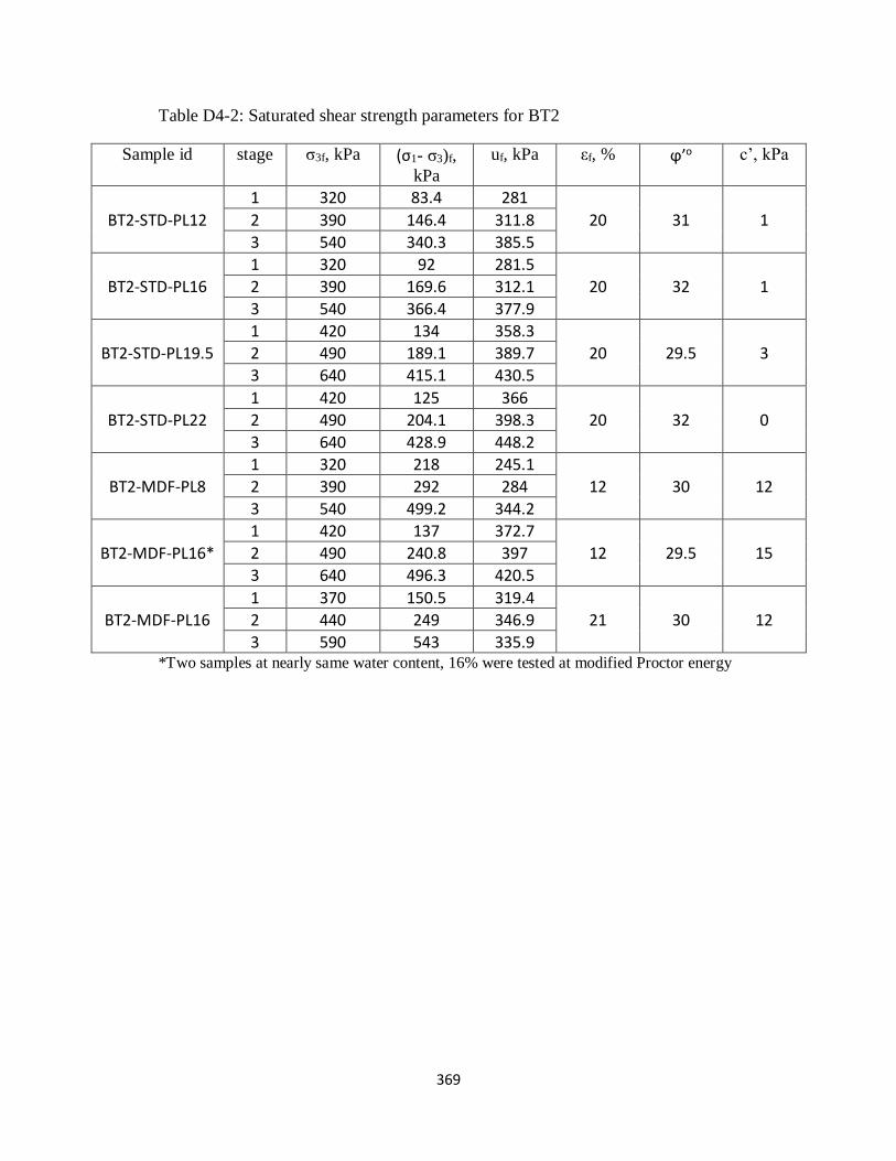
369

Table D4-2: Saturated shear strength parameters for BT2


kPa


BT2-STD-PL12

1 320 83.4 281

20 31 1 2 390 146.4 311.8

3 540 340.3 385.5

BT2-STD-PL16

1 320 92 281.5

20 32 1 2 390 169.6 312.1

3 540 366.4 377.9

BT2-STD-PL19.5

1 420 134 358.3

20 29.5 3 2 490 189.1 389.7

3 640 415.1 430.5

BT2-STD-PL22

1 420 125 366

20 32 0 2 490 204.1 398.3

3 640 428.9 448.2

BT2-MDF-PL8

1 320 218 245.1

12 30 12 2 390 292 284

3 540 499.2 344.2

BT2-MDF-PL16*

1 420 137 372.7

12 29.5 15 2 490 240.8 397

3 640 496.3 420.5

BT2-MDF-PL16

1 370 150.5 319.4

21 30 12 2 440 249 346.9

3 590 543 335.9 *Two samples at nearly same water content, 16% were tested at modified Proctor energy

370

Table D4-3: Saturated shear strength parameters for JF1


kPa


JF1-STD-PL13

1 420 98.2 372.6

20 27.5 9 2 490 166 404.3

3 640 333.3 445.6

JF1-STD-PL18

1 420 78 384

20 26.5 7 2 490 155 411

3 640 338.6 447.1

JF1-STD-PL22

1 420 116.2 362.2

20 26.5 7 2 490 192.3 394.1

3 640 395.7 449

JF1-MDF-PL9

1 320 103 268

19 28 15 2 390 149.3 304.4

3 540 416 328

JF1-MDF-PL15

1 420 97 275

20 25.5 12 2 490 168.2 404.1

3 640 397 398.1

JF1-MDF-PL19.5

1 420 142.3 367.9

12 28 15 2 490 234.5 394.4

3 640 449.5 414.4

371

Table D4-4: Saturated shear strength parameters for JF2


kPa


JF2-STD-PL10

1 370 96.4 326.2

12.2 31 1 2 440 134.4 358.7

3 590 362.6 419.8

JF2-STD-PL14

1 170 99.2 116.7

16.1 31 0 2 240 197.8 144.8

3 390 413.3 195.5

JF2-STD-PL16

1 320 87.6 269.3

16 30 3 2 390 173.5 348.0

3 540 391 348.0

JF2-STD-PL18

1 220 98.1 178.8

16.1 30 5 2 290 198.2 204.7

3 440 428.2 233.2

JF2-STD-PL20*

1 310 113 263.3

14.3 24* 10* 2 390 169.3 295.6

3 540 323.1 325.4

JF2-MDF-PL8

1 420 117.5 372.6

20 29 8 2 490 207.5 397.5

3 640 481 398.7

JF2-MDF-PL11

1 320 128.5 269.6

14.7 30 8 2 390 237.3 292.8

3 540 509.3 299.5

JF2-MDF-PL13.5

1 190 123 143.0

14.0 29 12 2 260 240.4 160.0

3 410 463.6 187.6

JF2-MDF-PL15

1 370 144.4 308.0

12.6 29 10 2 440 260 337.2

3 590 473.3 359.3

JF2-MDF-PL17

1 370 154 314.1

12.2 30 10 2 440 240.2 341.7

3 590 538 337.8

*Result is suspect.

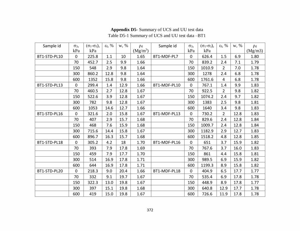
372

Appendix D5- Summary of UCS and UU test data

Table D5-1 Summary of UCS and UU test data –BT1

Sample id σ3,

kPa

(σ1-σ3),

kPa

εf, % w, % ρd

(Mg/m3) Sample id σ3,

kPa

(σ1-σ3),

kPa

εf, % w, % ρd

(Mg/m3)

BT1-STD-PL10 0 225.8 1.1 10 1.65 BT1-MDF-PL7 0 626.4 1.5 6.9 1.80

70 452.7 2.5 9.9 1.66 70 839.2 2.4 7.1 1.79

150 548 2.9 9.8 1.64 150 1010.9 2 7.0 1.78

300 860.2 12.8 9.8 1.64 300 1278 2.4 6.8 1.78

600 1352 15.8 9.8 1.66 600 1761.6 4 6.8 1.78

BT1-STD-PL13 0 299.4 1.4 12.9 1.66 BT1-MDF-PL10 0 767.1 1.4 9.9 1.83

70 460.5 2.7 12.8 1.67 70 922.5 2 9.8 1.82

150 522.6 3.9 12.8 1.67 150 1074.2 2.4 9.7 1.82

300 782 9.8 12.8 1.67 300 1383 2.5 9.8 1.81

600 1053 14.6 12.7 1.66 600 1640 3.4 9.8 1.83

BT1-STD-PL16 0 321.6 2.0 15.8 1.67 BT1-MDF-PL13 0 730.2 2 12.8 1.83

70 407 2.9 15.7 1.68 70 829.6 2.4 12.8 1.84

150 468 7.6 15.9 1.68 150 1009.7 2.4 12.8 1.84

300 715.6 14.4 15.8 1.67 300 1182.9 2.9 12.7 1.83

600 896.7 16.3 15.7 1.68 600 1518.2 4.8 12.8 1.85

BT1-STD-PL18 0 305.2 4.2 18 1.70 BT1-MDF-PL16 0 651 3.7 15.9 1.82

70 393 7.9 17.8 1.69 70 767.6 3.7 16.0 1.83

150 459 7.9 17.7 1.70 150 861 4.4 15.8 1.81

300 514 16.9 17.8 1.71 300 989.5 6.9 15.9 1.82

600 644 16.9 17.8 1.71 600 1199.3 8.9 15.8 1.82

BT1-STD-PL20 0 218.3 9.0 20.4 1.66 BT1-MDF-PL18 0 404.9 6.5 17.7 1.77

70 332 9.1 19.7 1.67 70 535.4 6.9 17.8 1.78

150 322.3 13.0 19.8 1.67 150 448.9 8.9 17.8 1.77

300 397 15.1 19.8 1.68 300 640.8 12.9 17.7 1.78

600 419 15.0 19.8 1.67 600 726.6 11.9 17.8 1.78

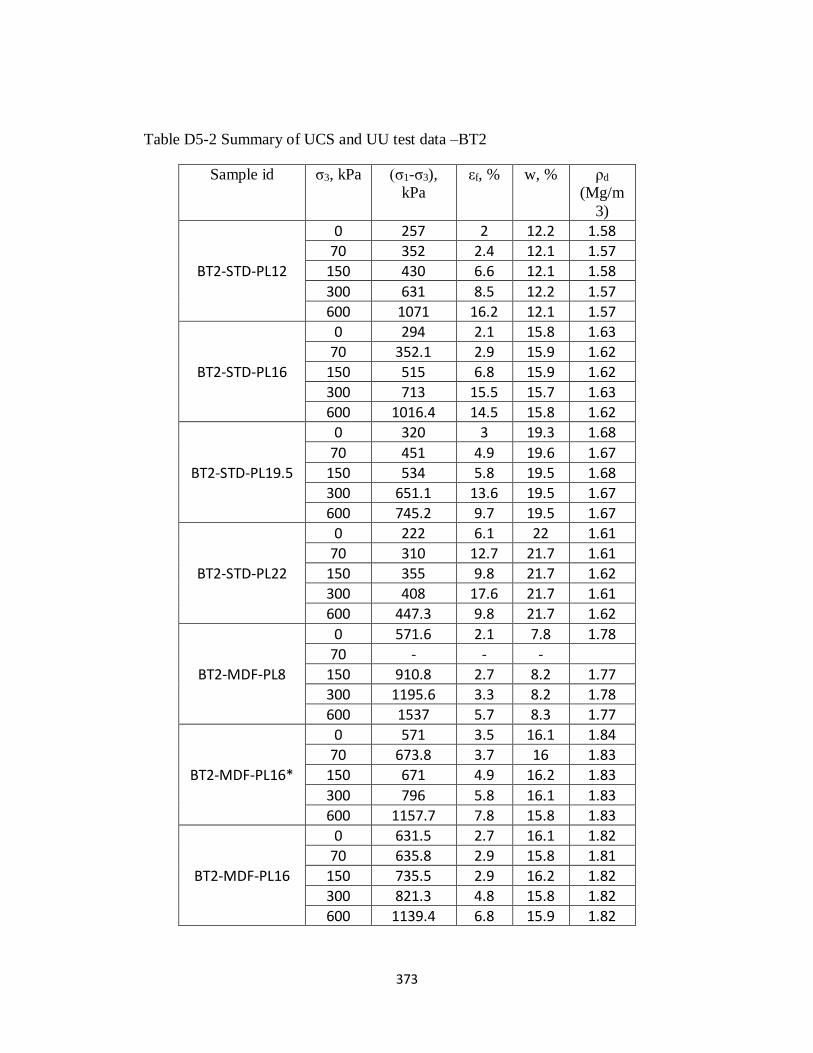
373

Table D5-2 Summary of UCS and UU test data –BT2

Sample id σ3, kPa (σ1-σ3),

kPa

εf, % w, % ρd

(Mg/m

3)

BT2-STD-PL12

0 257 2 12.2 1.58

70 352 2.4 12.1 1.57

150 430 6.6 12.1 1.58

300 631 8.5 12.2 1.57

600 1071 16.2 12.1 1.57

BT2-STD-PL16

0 294 2.1 15.8 1.63

70 352.1 2.9 15.9 1.62

150 515 6.8 15.9 1.62

300 713 15.5 15.7 1.63

600 1016.4 14.5 15.8 1.62

BT2-STD-PL19.5

0 320 3 19.3 1.68

70 451 4.9 19.6 1.67

150 534 5.8 19.5 1.68

300 651.1 13.6 19.5 1.67

600 745.2 9.7 19.5 1.67

BT2-STD-PL22

0 222 6.1 22 1.61

70 310 12.7 21.7 1.61

150 355 9.8 21.7 1.62

300 408 17.6 21.7 1.61

600 447.3 9.8 21.7 1.62

BT2-MDF-PL8

0 571.6 2.1 7.8 1.78

70 - - -

150 910.8 2.7 8.2 1.77

300 1195.6 3.3 8.2 1.78

600 1537 5.7 8.3 1.77

BT2-MDF-PL16*

0 571 3.5 16.1 1.84

70 673.8 3.7 16 1.83

150 671 4.9 16.2 1.83

300 796 5.8 16.1 1.83

600 1157.7 7.8 15.8 1.83

BT2-MDF-PL16

0 631.5 2.7 16.1 1.82

70 635.8 2.9 15.8 1.81

150 735.5 2.9 16.2 1.82

300 821.3 4.8 15.8 1.82

600 1139.4 6.8 15.9 1.82

374

Table D5-3 Summary of UCS and UU test data –JF1

Sample id σ3,

kPa

(σ1-σ3),

kPa

εf, % w, % ρd

(Mg/m3)

JF1-STD-PL13

0 236.3 1.2 12.9 1.61

70 422 2.3 13.0 1.60

150 464 2.9 12.8 1.59

300 773.9 7.8 12.8 1.59

600 1243.7 17.4 12.9 1.60

JF1-STD-PL18

0 341.4 1.9 17.8 1.64

70 422.8 2.9 17.7 1.63

150 496.2 4.8 17.7 1.63

300 770.3 13.4 17.7 1.63

600 939.6 18.4 17.7 1.64

JF1-STD-PL22

0 244 9.9 21.8 1.63

70 243.2 11 21.6 1.63

150 300.7 17.8 21.5 1.63

300 386.5 19 21.7 1.63

600 436.6 19.8 21.5 1.64

JF1-MDF-PL9

0 612.1 1.5 9.1 1.75

70 822.8 1.5 9.1 1.75

150 1048 2.5 9.2 1.75

300 1493.6 2.5 9.1 1.74

600 1868.1 5 9.2 1.74

JF1-MDF-PL15

0 661.4 1.8 14.5 1.78

70 788.2 2.22 14.6 1.79

150 1004.4 2.9 14.6 1.78

300 1184.3 4.3 14.6 1.80

600 1412.6 8.7 14.6 1.79

JF1-MDF-PL19.5

0 578.6 6 19.2 1.74

70 606 6.5 19.1 1.74

150 654 9 19.1 1.75

300 744 12 19.1 1.74

600 808.5 10 19.1 1.74

375

Table D5-4 Summary of UCS and UU test data –JF2

Sample id σ3,

kPa

(σ1-σ3),

kPa

εf, % w, % ρd

(Mg/m3

)

Sample id σ3,

kPa

(σ1-σ3),

kPa

εf, % w, % ρd

(Mg/m3)

JF2-STD-PL10 0 225.1 1.4 9.7 1.72 JF2-MDF-PL8 0 560.3 1.8 8.2 1.83

70 542.4 3.0 10.0 1.71 70 745.9 2.1 8.1 1.84

150 697.2 3.6 10.1 1.72 150 1019.7 2.7 8.2 1.83

300 960.3 6.1 9.7 1.72 300 1216.4 2.7 8.2 1.83

600 1602.4 14.3 9.9 1.72 600 1640.8 5.8 8.2 1.84

JF2-STD-PL14 0 304.3 1.6 14.0 1.73 JF2-MDF-PL11 0 671 1.8 11 1.86

70 550 2.9 13.7 1.74 70 769 1.8 11 1.85

150 673 4.9 13.6 1.74 150 927 2.4 11 1.85

300 892 11.8 13.7 1.73 300 1239 3.3 11 1.85

600 1224 11.9 13.8 1.74 600 1650 7.3 11 1.86

JF2-STD-PL16 0 347.8 3.1 16.0 1.76 JF2-MDF-PL13.5 0 643.2 2.4 13.5 1.88

70 476.5 5.2 15.9 1.77 70 -

150 567.1 7.8 16.0 1.76 150 880 3.3 13.4 1.87

300 719.5 11.7 16.2 1.76 300 1046.8 5.7 13.5 1.87

600 946.5 11.2 16.2 1.76 600 1305.4 7.6 13.3 1.87

JF2-STD-PL18 0 331.3 4.1 17.6 1.75 JF2-MDF-PL15 0 593 3.2 15.1 1.85

70 370.9 10.5 17.7 1.75 70 561 3.4 15.2 1.84

150 444 10.6 17.7 1.74 150 741 4.3 15.2 1.84

300 558.7 11.5 17.7 1.74 300 956.3 6.7 15.3 1.85

600 748.5 16.4 17.7 1.75 600 1249 11.5 15.3 1.85

JF2-STD-PL20 0 225.7 10.7 19.7 1.71 JF2-MDF-PL17 0 411.5 5.7 16.9 1.80

70 245.9 11.6 20.0 1.71 70 465.4 7.6 17.0 1.80

150 268.9 15.5 20.2 1.72 150 552.5 9.5 17.0 1.79

300 319.4 23.4 20.1 1.72 300 631.5 11.0 17.2 1.80

600 312.6 15.4 19.9 1.72 600 7302 20.0 17.2 1.78

376

Appendix D6- UC and UU Mohr circles fitted with tangents inclined at φ’

-1000

0

1000

2000

-1000 0 1000 2000 3000

τ(k

Pa)

σ(kPa)

BT1-STD-PL13

-1000

0

1000

2000

-1000 0 1000 2000 3000

τ(k

Pa)

σ(kPa)

BT1-STD-PL16

-1000

0

1000

2000

-1000 0 1000 2000 3000

τ(k

Pa)

σ(kPa)

BT1-STD-PL18

-1000

0

1000

2000

-1000 0 1000 2000 3000

τ(k

Pa)

σ(kPa)

BT1-MDF-PL10

-1000

0

1000

2000

-1000 0 1000 2000 3000

τ(k

Pa)

σ(kPa)

BT1-MDF-PL13

-1000

0

1000

2000

-1000 0 1000 2000 3000

τ(k

Pa)

σ(kPa)

BT1-MDF-PL16

Figure D6-1: UC and UU Mohr circles fitted with tangents inclined at φ’- BT1

377

-1000

0

1000

2000

-1000 0 1000 2000 3000

τ(k

Pa)

σ(kPa)

JF1-STD-PL18

-1000

0

1000

2000

-1000 0 1000 2000 3000

τ(k

Pa)

σ(kPa)

JF1-STD-PL22

-1000

0

1000

2000

-1000 0 1000 2000 3000

τ(k

Pa)

σ(kPa)

JF1-STD-PL13

-1000

0

1000

2000

-1000 0 1000 2000 3000

τ(k

Pa)

σ(kPa)

JF1-MDF-PL15

-1000

0

1000

2000

-1000 0 1000 2000 3000

τ(k

Pa)

σ(kPa)

JF1-MDF-PL19.5

-1000

0

1000

2000

-1000 0 1000 2000 3000

τ(k

Pa)

σ(kPa)

JF1-STD-PL13

378

-1000

0

1000

2000

-1000 0 1000 2000 3000

τ(k

Pa)

σ(kPa)

JF2-STD-PL14

-1000

0

1000

2000

-1000 0 1000 2000 3000

τ(k

Pa)

σ(kPa)

JF2-STD-PL16

-1000

0

1000

2000

-1000 0 1000 2000 3000

τ(k

Pa)

σ(kPa)

JF2-STD-PL18

-1000

0

1000

2000

-1000 0 1000 2000 3000

τ(k

Pa)

σ(kPa)

JF2-MDF-PL13.5

-1000

0

1000

2000

-1000 0 1000 2000 3000

τ(k

Pa)

σ(kPa)

JF2-MDF-PL8

-1000

0

1000

2000

-1000 0 1000 2000 3000

τ(k

Pa)

σ(kPa)

JF2-MDF-PL11

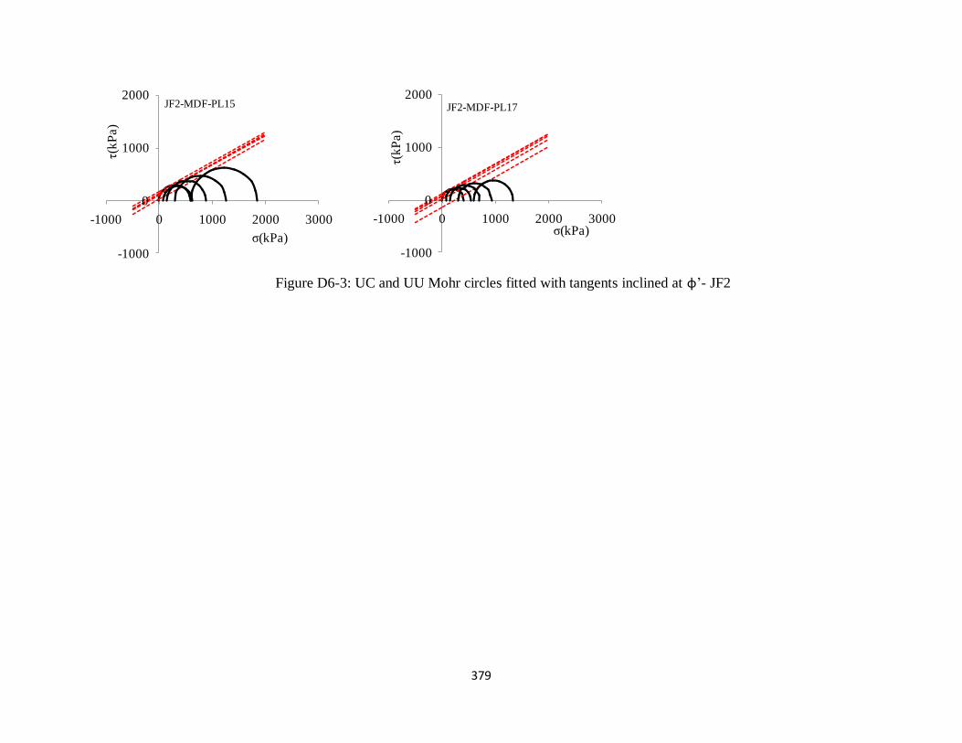
379

Figure D6-3: UC and UU Mohr circles fitted with tangents inclined at φ’- JF2

-1000

0

1000

2000

-1000 0 1000 2000 3000

τ(k

Pa)

σ(kPa)

JF2-MDF-PL15

-1000

0

1000

2000

-1000 0 1000 2000 3000

τ(k

Pa)

σ(kPa)

JF2-MDF-PL17

380

Figure D6-3: UC and UU Mohr circles fitted with tangents inclined at φ’- BT2

-1000

0

1000

2000

-1000 0 1000 2000 3000

τ(k

Pa)

σ(kPa)

BT2-STD-PL19.5

-1000

0

1000

2000

-1000 0 1000 2000 3000

τ(k

Pa)

σ(kPa)

BT2-STD-PL16

-1000

0

1000

2000

-1000 0 1000 2000 3000

τ(k

Pa)

σ(kPa)

BT2-STD-PL13

-1000

0

1000

2000

-1000 0 1000 2000 3000

τ(k

Pa)

σ(kPa)

BT2-MDF-PL16

-1000

0

1000

2000

-1000 0 1000 2000 3000

τ(k

Pa)

σ(kPa)

BT2-MDF-PL16*

suction, hydraulic and strength properties of compacted soils thesis - kizza... · the two major...

Documents