subsystems of second order arithmetic

CUUS579-Simpson April 1, 2009 21:45 978 0 521 88439 6

ii

This page intentionally left blank


Subsystems of Second Order ArithmeticSecond Edition

Foundations of mathematics is the study of the most basic concepts and logicalstructure of mathematics, with an eye to the unity of human knowledge. Almost allof the problems studied in this book are motivated by an overriding foundationalquestion: What are the appropriate axioms for mathematics? Through a series ofcase studies, these axioms are examined to prove particular theorems in core mathe-matical areas such as algebra, analysis, and topology, focusing on the language ofsecond order arithmetic, the weakest language rich enough to express and developthe bulk of mathematics.

In many cases, if a mathematical theorem is proved from appropriately weakset existence axioms, then the axioms will be logically equivalent to the theorem.Furthermore, only a few specific set existence axioms arise repeatedly in thiscontext, which in turn correspond to classical foundational programs. This is thetheme of reverse mathematics, which dominates the first half of the book. Thesecond part focuses on models of these and other subsystems of second orderarithmetic. Additional results are presented in an appendix.

Stephen G. Simpson is a mathematician and professor at Pennsylvania State Uni-versity. The winner of the Grove Award for Interdisciplinary Research Initia-tion, Simpson specializes in research involving mathematical logic, foundationsof mathematics, and combinatorics.

i


ii


PERSPECTIVES IN LOGIC

The Perspectives in Logic series publishes substantial, high-quality books whosecentral theme lies in any area or aspect of logic. Works that present new materialnot available in book form are particularly welcome. The series ranges from intro-ductory texts suitable for beginning graduate courses to specialized monographsat the frontiers of research. Each book offers an illuminating perspective for itsintended audience.

The series has its origins in the old Perspectives in Mathematical Logic seriesedited by the -Group for “Mathematische Logik” of the Heidelberger Akademieder Wissenchaften, whose beginnings date back to the 1960s. The Association forSymbolic Logic has assumed editorial responsibility for the series and changed itsname to reflect its interest in books that span the full range of disciplines in whichlogic plays an important role.

Pavel Pudlak, Managing EditorMathematical Institute of the Academy of Sciences of the Czech Republic

Editorial Board

Michael BenediktDepartment of Computing Science, University of Oxford

Michael GlanzbergDepartment of Philosophy, University of California, Davis

Carl G. Jockusch, Jr.Department of Mathematics, University of Illinois at Urbana-Champaign

Michael RathjenSchool of Mathematics, University of Leeds

Thomas ScanlonDepartment of Mathematics, University of California, Berkeley

Simon ThomasDepartment of Mathematics, Rutgers University

ASL PublisherRichard A. ShoreDepartment of Mathematics, Cornell University

For more information, see http://www.aslonline.org/books perspectives.html

iii


iv


PERSPECTIVES IN LOGIC

Subsystems of Second Order Arithmetic

Second Edition

STEPHEN G. SIMPSON

Pennsylvania State University

association for symbolic logic

v

CAMBRIDGE UNIVERSITY PRESS

Cambridge, New York, Melbourne, Madrid, Cape Town, Singapore,

São Paulo, Delhi, Dubai, Tokyo

Cambridge University Press

The Edinburgh Building, Cambridge CB2 8RU, UK

First published in print format

ISBN-13 978-0-521-88439-6

ISBN-13 978-0-511-57985-1

© The Association for Symbolic Logic 2009

2009

Information on this title: www.cambridge.org/9780521884396

This publication is in copyright. Subject to statutory exception and to the

provision of relevant collective licensing agreements, no reproduction of any part

may take place without the written permission of Cambridge University Press.

Cambridge University Press has no responsibility for the persistence or accuracy

of urls for external or third-party internet websites referred to in this publication,

and does not guarantee that any content on such websites is, or will remain,

accurate or appropriate.

Published in the United States of America by Cambridge University Press, New York

www.cambridge.org

eBook (EBL)

Hardback

i

i

i

i

i

i

i

i

CONTENTS

List of Tables . . . . . . . . . . . . . . . . . . . . . . . . . . . . . . . . . . . . . . . . . . . . . . . . . . . xi

Preface . . . . . . . . . . . . . . . . . . . . . . . . . . . . . . . . . . . . . . . . . . . . . . . . . . . . . . . . . . xiii

Acknowledgments . . . . . . . . . . . . . . . . . . . . . . . . . . . . . . . . . . . . . . . . . . . . . . xv

Chapter I. Introduction . . . . . . . . . . . . . . . . . . . . . . . . . . . . . . . . . . . . . . 1I.1. The Main Question . . . . . . . . . . . . . . . . . . . . . . . . . . . . . . . . . . . . 1I.2. Subsystems of Z2 . . . . . . . . . . . . . . . . . . . . . . . . . . . . . . . . . . . . . . 2I.3. The System ACA0 . . . . . . . . . . . . . . . . . . . . . . . . . . . . . . . . . . . . . 6I.4. Mathematics within ACA0 . . . . . . . . . . . . . . . . . . . . . . . . . . . . . 9I.5. Π11-CA0 and Stronger Systems . . . . . . . . . . . . . . . . . . . . . . . . . . 16I.6. Mathematics within Π11-CA0 . . . . . . . . . . . . . . . . . . . . . . . . . . . 19I.7. The System RCA0 . . . . . . . . . . . . . . . . . . . . . . . . . . . . . . . . . . . . . 23I.8. Mathematics within RCA0 . . . . . . . . . . . . . . . . . . . . . . . . . . . . . 27I.9. Reverse Mathematics . . . . . . . . . . . . . . . . . . . . . . . . . . . . . . . . . . 32I.10. The SystemWKL0 . . . . . . . . . . . . . . . . . . . . . . . . . . . . . . . . . . . . . 35I.11. The System ATR0 . . . . . . . . . . . . . . . . . . . . . . . . . . . . . . . . . . . . . . 38I.12. The Main Question, Revisited. . . . . . . . . . . . . . . . . . . . . . . . . . 42I.13. Outline of Chapters II through X. . . . . . . . . . . . . . . . . . . . . . . 43I.14. Conclusions . . . . . . . . . . . . . . . . . . . . . . . . . . . . . . . . . . . . . . . . . . . 60

Part A. Development of Mathematics within Subsystems of Z2

Chapter II. Recursive Comprehension . . . . . . . . . . . . . . . . . . . . . . . . . 63II.1. The Formal System RCA0 . . . . . . . . . . . . . . . . . . . . . . . . . . . . . . 63II.2. Finite Sequences . . . . . . . . . . . . . . . . . . . . . . . . . . . . . . . . . . . . . . 65II.3. Primitive Recursion . . . . . . . . . . . . . . . . . . . . . . . . . . . . . . . . . . . 69II.4. The Number Systems . . . . . . . . . . . . . . . . . . . . . . . . . . . . . . . . . . 73II.5. Complete Separable Metric Spaces . . . . . . . . . . . . . . . . . . . . . 78II.6. Continuous Functions . . . . . . . . . . . . . . . . . . . . . . . . . . . . . . . . . 84II.7. More on Complete Separable Metric Spaces . . . . . . . . . . . . 88II.8. Mathematical Logic . . . . . . . . . . . . . . . . . . . . . . . . . . . . . . . . . . . 92II.9. Countable Fields . . . . . . . . . . . . . . . . . . . . . . . . . . . . . . . . . . . . . . 96

vii

i

i

i

i

i

i

i

i

viii Contents

II.10. Separable Banach Spaces . . . . . . . . . . . . . . . . . . . . . . . . . . . . . . 99II.11. Conclusions . . . . . . . . . . . . . . . . . . . . . . . . . . . . . . . . . . . . . . . . . . . 103

Chapter III. Arithmetical Comprehension . . . . . . . . . . . . . . . . . . . . . 105III.1. The Formal System ACA0 . . . . . . . . . . . . . . . . . . . . . . . . . . . . . . 105III.2. Sequential Compactness . . . . . . . . . . . . . . . . . . . . . . . . . . . . . . . 106III.3. Strong Algebraic Closure . . . . . . . . . . . . . . . . . . . . . . . . . . . . . . 110III.4. Countable Vector Spaces. . . . . . . . . . . . . . . . . . . . . . . . . . . . . . . 112III.5. Maximal Ideals in Countable Commutative Rings. . . . . . . 115III.6. Countable Abelian Groups . . . . . . . . . . . . . . . . . . . . . . . . . . . . 118III.7. Konig’s Lemma and Ramsey’s Theorem . . . . . . . . . . . . . . . . 121III.8. Conclusions . . . . . . . . . . . . . . . . . . . . . . . . . . . . . . . . . . . . . . . . . . . 125

Chapter IV. Weak Konig’s Lemma . . . . . . . . . . . . . . . . . . . . . . . . . . . . . 127IV.1. The Heine/Borel Covering Lemma . . . . . . . . . . . . . . . . . . . . . 127IV.2. Properties of Continuous Functions . . . . . . . . . . . . . . . . . . . . 133IV.3. The Godel Completeness Theorem . . . . . . . . . . . . . . . . . . . . . 139IV.4. Formally Real Fields . . . . . . . . . . . . . . . . . . . . . . . . . . . . . . . . . . 141IV.5. Uniqueness of Algebraic Closure . . . . . . . . . . . . . . . . . . . . . . . 144IV.6. Prime Ideals in Countable Commutative Rings . . . . . . . . . . 146IV.7. Fixed Point Theorems . . . . . . . . . . . . . . . . . . . . . . . . . . . . . . . . . 149IV.8. Ordinary Differential Equations . . . . . . . . . . . . . . . . . . . . . . . . 154IV.9. The Separable Hahn/Banach Theorem . . . . . . . . . . . . . . . . . 160IV.10. Conclusions . . . . . . . . . . . . . . . . . . . . . . . . . . . . . . . . . . . . . . . . . . . 165

Chapter V. Arithmetical Transfinite Recursion . . . . . . . . . . . . . . 167V.1. Countable Well Orderings; Analytic Sets . . . . . . . . . . . . . . . . 167V.2. The Formal System ATR0 . . . . . . . . . . . . . . . . . . . . . . . . . . . . . . 173V.3. Borel Sets . . . . . . . . . . . . . . . . . . . . . . . . . . . . . . . . . . . . . . . . . . . . . 178V.4. Perfect Sets; Pseudohierarchies . . . . . . . . . . . . . . . . . . . . . . . . . 185V.5. Reversals . . . . . . . . . . . . . . . . . . . . . . . . . . . . . . . . . . . . . . . . . . . . . 189V.6. Comparability of Countable Well Orderings . . . . . . . . . . . . 195V.7. Countable Abelian Groups . . . . . . . . . . . . . . . . . . . . . . . . . . . . 199V.8. Σ01 and ∆

01 Determinacy . . . . . . . . . . . . . . . . . . . . . . . . . . . . . . . . 203

V.9. The Σ01 and ∆01 Ramsey Theorems . . . . . . . . . . . . . . . . . . . . . . 210

V.10. Conclusions . . . . . . . . . . . . . . . . . . . . . . . . . . . . . . . . . . . . . . . . . . . 215

Chapter VI. Π11 Comprehension . . . . . . . . . . . . . . . . . . . . . . . . . . . . . . . . 217VI.1. Perfect Kernels . . . . . . . . . . . . . . . . . . . . . . . . . . . . . . . . . . . . . . . . 217VI.2. Coanalytic Uniformization . . . . . . . . . . . . . . . . . . . . . . . . . . . . 221VI.3. Coanalytic Equivalence Relations . . . . . . . . . . . . . . . . . . . . . . 225VI.4. Countable Abelian Groups . . . . . . . . . . . . . . . . . . . . . . . . . . . . 230VI.5. Σ01 ∧Π01 Determinacy . . . . . . . . . . . . . . . . . . . . . . . . . . . . . . . . . . 232VI.6. The ∆02 Ramsey Theorem . . . . . . . . . . . . . . . . . . . . . . . . . . . . . . 236VI.7. Stronger Set Existence Axioms . . . . . . . . . . . . . . . . . . . . . . . . . 239VI.8. Conclusions . . . . . . . . . . . . . . . . . . . . . . . . . . . . . . . . . . . . . . . . . . . 240

i

i

i

i

i

i

i

i

Contents ix

Part B. Models of Subsystems of Z2

Chapter VII. â-Models . . . . . . . . . . . . . . . . . . . . . . . . . . . . . . . . . . . . . . . . 243VII.1. The Minimum â-Model of Π11-CA0 . . . . . . . . . . . . . . . . . . . . . 244VII.2. Countable Coded â-Models. . . . . . . . . . . . . . . . . . . . . . . . . . . . 248VII.3. A Set-Theoretic Interpretation of ATR0 . . . . . . . . . . . . . . . . . 258VII.4. Constructible Sets and Absoluteness . . . . . . . . . . . . . . . . . . . 272VII.5. Strong Comprehension Schemes . . . . . . . . . . . . . . . . . . . . . . . 286VII.6. Strong Choice Schemes . . . . . . . . . . . . . . . . . . . . . . . . . . . . . . . . 294VII.7. â-Model Reflection . . . . . . . . . . . . . . . . . . . . . . . . . . . . . . . . . . . . 303VII.8. Conclusions . . . . . . . . . . . . . . . . . . . . . . . . . . . . . . . . . . . . . . . . . . . 307

Chapter VIII. ù-Models . . . . . . . . . . . . . . . . . . . . . . . . . . . . . . . . . . . . . . . 309VIII.1. ù-Models of RCA0 and ACA0 . . . . . . . . . . . . . . . . . . . . . . . . . . 310VIII.2. Countable Coded ù-Models ofWKL0 . . . . . . . . . . . . . . . . . . 314VIII.3. Hyperarithmetical Sets . . . . . . . . . . . . . . . . . . . . . . . . . . . . . . . . 322VIII.4. ù-Models of Σ11 Choice . . . . . . . . . . . . . . . . . . . . . . . . . . . . . . . . 333VIII.5. ù-Model Reflection and Incompleteness . . . . . . . . . . . . . . . . 342VIII.6. ù-Models of Strong Systems . . . . . . . . . . . . . . . . . . . . . . . . . . . 348VIII.7. Conclusions . . . . . . . . . . . . . . . . . . . . . . . . . . . . . . . . . . . . . . . . . . . 356

Chapter IX. Non-ù-Models . . . . . . . . . . . . . . . . . . . . . . . . . . . . . . . . . . . 359IX.1. The First Order Parts of RCA0 and ACA0 . . . . . . . . . . . . . . . 360IX.2. The First Order Part ofWKL0 . . . . . . . . . . . . . . . . . . . . . . . . . . 365IX.3. A Conservation Result for Hilbert’s Program . . . . . . . . . . . 369IX.4. SaturatedModels . . . . . . . . . . . . . . . . . . . . . . . . . . . . . . . . . . . . . 379IX.5. Gentzen-Style Proof Theory . . . . . . . . . . . . . . . . . . . . . . . . . . . 386IX.6. Conclusions . . . . . . . . . . . . . . . . . . . . . . . . . . . . . . . . . . . . . . . . . . . 388

Appendix

Chapter X. Additional Results . . . . . . . . . . . . . . . . . . . . . . . . . . . . . . . 391X.1. Measure Theory . . . . . . . . . . . . . . . . . . . . . . . . . . . . . . . . . . . . . . . 391X.2. Separable Banach Spaces . . . . . . . . . . . . . . . . . . . . . . . . . . . . . . 396X.3. Countable Combinatorics . . . . . . . . . . . . . . . . . . . . . . . . . . . . . . 399X.4. Reverse Mathematics for RCA0 . . . . . . . . . . . . . . . . . . . . . . . . . 405X.5. Conclusions . . . . . . . . . . . . . . . . . . . . . . . . . . . . . . . . . . . . . . . . . . . 407

Bibliography . . . . . . . . . . . . . . . . . . . . . . . . . . . . . . . . . . . . . . . . . . . . . . . . . . . . 409

Index . . . . . . . . . . . . . . . . . . . . . . . . . . . . . . . . . . . . . . . . . . . . . . . . . . . . . . . . . . . . 425

i

i

i

i

i

i

i

i

i

i

i

i

i

i

i

i

LIST OF TABLES

1 Foundational programs and the five basic systems. . . . . . . . . . . . . . 43

2 An overview of the entire book. . . . . . . . . . . . . . . . . . . . . . . . . . . . . . . . 44

3 Ordinary mathematics within the five basic systems. . . . . . . . . . . . . 45

4 Models of subsystems of Z2. . . . . . . . . . . . . . . . . . . . . . . . . . . . . . . . . . . 54

xi

i

i

i

i

i

i

i

i

i

i

i

i

i

i

i

i

PREFACE

Foundations of mathematics is the study of the most basic concepts andlogical structure ofmathematics, with an eye to the unity of human knowl-edge. Among the most basic mathematical concepts are: number, shape,set, function, algorithm, mathematical axiom, mathematical definition,and mathematical proof. Typical questions in foundations of mathemat-ics include: What is a number? What is a shape? What is a set? What isa function? What is an algorithm? What is a mathematical axiom? Whatis a mathematical definition? What is a mathematical proof ? What arethe most basic concepts of mathematics? What is the logical structure ofmathematics? What are the appropriate axioms for numbers? What arethe appropriate axioms for shapes? What are the appropriate axioms forsets? What are the appropriate axioms for functions?Obviously, foundations ofmathematics is a subject of the greatestmath-ematical and philosophical importance. Beyond this, foundations ofmathematics is a rich subject with a long history, going back to Aristotleand Euclid and continuing in the hands of outstanding modern figuressuch as Descartes, Cauchy, Weierstraß, Dedekind, Peano, Frege, Russell,Cantor, Hilbert, Brouwer, Weyl, vonNeumann, Skolem, Tarski, Heyting,and Godel. An excellent reference for the modern era in foundations ofmathematics is van Heijenoort [272].In the late 19th and early 20th centuries, virtually all leadingmathemati-cians were intensely interested in foundations of mathematics and spokeand wrote extensively on this subject. Today that is no longer the case.Regrettably, foundations of mathematics is now out of fashion. Today,most of the leading mathematicians are ignorant of foundations and focusmostly on structural questions. Today, foundations of mathematics is outof favor even amongmathematical logicians, the majority of whom preferto concentrate on methodological or other non-foundational issues.This book is a contribution to foundations of mathematics. Almostall of the problems studied in this book are motivated by an overridingfoundational question: What are the appropriate axioms for mathematics?We undertake a series of case studies to discover which are the appropriateaxioms for proving particular theorems in core mathematical areas such

xiii

i

i

i

i

i

i

i

i

xiv Preface

as algebra, analysis, and topology. We focus on the language of secondorder arithmetic, because that language is the weakest one that is richenough to express and develop the bulk of core mathematics. It turns outthat, in many particular cases, if a mathematical theorem is proved fromappropriately weak set existence axioms, then the axioms will be logicallyequivalent to the theorem. Furthermore, only a few specific set existenceaxioms arise repeatedly in this context: recursive comprehension, weakKonig’s lemma, arithmetical comprehension, arithmetical transfinite re-cursion, Π11 comprehension; corresponding to the formal systems RCA0,WKL0, ACA0, ATR0, Π

11-CA0; which in turn correspond to classical foun-

dational programs: constructivism, finitistic reductionism, predicativism,and predicative reductionism. This is the theme of Reverse Mathematics,which dominates Part A of this book. Part B focuses on models of theseand other subsystems of second order arithmetic. Additional results arepresented in an appendix.The formalization of mathematics within second order arithmetic goesback to Dedekind and was developed by Hilbert and Bernays [115, sup-plement IV]. The present book may be viewed as a continuation ofHilbert/Bernays [115]. I hope that the present book will help to re-vive the study of foundations of mathematics and thereby earn for itself apermanent place in the history of the subject.The first edition of this book [249] was published in January 1999. Thesecond edition differs from the first only in that I have corrected sometypographical errors and updated some bibliographical entries. Recentadvances are in research papers by numerous authors,published inReverseMathematics 2001 [228] and in scholarly journals. The Web page for thisbook is http://www.math.psu.edu/simpson/sosoa/. I would like todevelop this Web page into a forum for research and scholarship, notonly in subsystems of second order arithmetic, but in foundations ofmathematics generally.

Stephen G. SimpsonNovember 2008

i

i

i

i

i

i

i

i

ACKNOWLEDGMENTS

Much of my work on subsystems of second order arithmetic has beencarried on in collaboration with my doctoral and postdoctoral adviseesat Berkeley and Penn State, including: Stephen Binns, Stephen Brackin,Douglas Brown, Natasha Dobrinen, Qi Feng, Fernando Ferreira, Maria-gnese Giusto, Kostas Hatzikiriakou, Jeffry Hirst, James Humphreys,Michael Jamieson, Alberto Marcone, Carl Mummert, Ju Rao, RickSmith, JohnSteel, KazuyukiTanaka,RobertVanWesep,GalenWeitkamp,Takeshi Yamazaki, and Xiaokang Yu. I also acknowledge the collabora-tion and encouragement of numerous colleagues including: Peter Aczel,Jeremy Avigad, Jon Barwise, Michael Beeson, Errett Bishop, AndreasBlass, Lenore Blum, Douglas Bridges, Wilfried Buchholz, John Burgess,Samuel Buss, Douglas Cenzer, Peter Cholak, Chi-Tat Chong, RolandoChuaqui, John Clemens, Peter Clote, Carlos Di Prisco, Rod Downey, AliEnayat, Herbert Enderton, Harvey Friedman, Robin Gandy, WilliamGasarch, Noam Greenberg, Petr Hajek, Valentina Harizanov, VictorHarnik, Leo Harrington, ChristophHeinatsch, Ward Henson, Peter Hin-man,DenisHirschfeldt, WilliamHoward,MartinHyland,Gerhard Jager,Haim Judah, Irving Kaplansky, Alexander Kechris, Jerome Keisler, Jef-frey Ketland, Bjørn Kjos-Hanssen, Stephen Kleene, Julia Knight, UlrichKohlenbach, Roman Kossak, Georg Kreisel, Antonın Kucera, MasahiroKumabe, Richard Laver, Steffen Lempp, Manuel Lerman, Azriel Levy,Alain Louveau, Angus Macintyre, Michael Makkai, Richard Mansfield,David Marker, Donald Martin, Adrian Mathias, Alex McAllister, Ken-neth McAloon, Timothy McNicholl, George Metakides, Joseph Mileti,Joseph Miller, Grigori Mints, Michael Mollerfeld, Antonio Montalban,Yiannis Moschovakis, Gert Muller, Roman Murawski, Jan Mycielski,Michael Mytilinaios, Anil Nerode, Andre Nies, Charles Parsons, Mar-ian Pour-El, Michael Rathjen, Jeffrey Remmel, Jean-Pierre Ressayre,Ian Richards, Hartley Rogers, Gerald Sacks, Ramez Sami, Andre Sce-drov, James Schmerl, Kurt Schutte, Helmut Schwichtenberg, Dana Scott,Saharon Shelah, John Shepherdson, Naoki Shioji, Joseph Shoenfield,Richard Shore, Wilfried Sieg, Jack Silver, Ksenija Simic, Theodore Sla-man, Craig Smorynski, Robert Soare, Reed Solomon, Robert Solovay,

xv

i

i

i

i

i

i

i

i

xvi Acknowledgments

Rick Sommer, Andrea Sorbi, Gaisi Takeuti, Dirk van Dalen, Lou vanden Dries, Daniel Velleman, Stanley Wainer, Dongping Yang, Yue Yang,and especially Solomon Feferman, Carl Jockusch, and Wolfram Pohlers.I acknowledge the help of various institutions including: the Alfred P.Sloan Foundation, the American Mathematical Society, the Associationfor Symbolic Logic, the Centre National de Recherche Scientifique, theDeutsche Forschungsgemeinschaft, theNational Science Foundation, theOmega Group, Oxford University, the Pennsylvania State University, theRaymondN.ShibleyFoundation, the ScienceResearchCouncil, Springer-Verlag, Stanford University, the University of California at Berkeley, theUniversity of Illinois at Urbana–Champaign, the University of Munich,the University of Paris, the University of Tennessee, and the VolkswagenFoundation.A preliminary version of this book was written with a software packagecalled MathText. I acknowledge important help from Robert Huff, theauthor of MathText, and Janet Huff. Padma Raghavan wrote additionalsoftware to help me convert the manuscript from MathText to LaTeX.The first edition [249] was published by Springer-Verlag with editorialassistance from the Association for Symbolic Logic. The second editionis being published by the Association for Symbolic Logic and CambridgeUniversity Press. I acknowledge help from Samuel Buss, Ward Henson,Reinhard Kahle, Steffen Lempp, Manuel Lerman, and Thanh-Ha LeThi.I thank my darling wife, Padma Raghavan, for her encouragement andemotional support while I was bringing this project to a conclusion, bothin 1997–1998 and again in 2008.

Stephen G. SimpsonNovember 2008

i

i

i

i

i

i

i

i

Chapter I

INTRODUCTION

I.1. The Main Question

The purpose of this book is to use the tools of mathematical logic tostudy certain problems in foundations of mathematics. We are especiallyinterested in the question of which set existence axioms are needed toprove the known theorems of mathematics.The scope of this initial question is very broad, but we can narrow itdown somewhat by dividing mathematics into two parts. On the one handthere is set-theoretic mathematics, and on the other hand there is whatwe call “non-set-theoretic” or “ordinary” mathematics. By set-theoreticmathematicswemean those branches of mathematics that were created bythe set-theoretic revolution which took place approximately a century ago.We have in mind such branches as general topology, abstract functionalanalysis, the study of uncountable discrete algebraic structures, and ofcourse abstract set theory itself.We identify as ordinary or non-set-theoretic that body of mathemat-ics which is prior to or independent of the introduction of abstract set-theoretic concepts. We have in mind such branches as geometry, numbertheory, calculus, differential equations, real and complex analysis, count-able algebra, the topology of complete separable metric spaces, mathe-matical logic, and computability theory.The distinction between set-theoretic and ordinary mathematics cor-responds roughly to the distinction between “uncountable mathematics”and “countable mathematics”. This formulation is valid if we stipulatethat “countable mathematics” includes the study of possibly uncountablecomplete separable metric spaces. (A metric space is said to be separableif it has a countable dense subset.) Thus for instance the study of continu-ous functions of a real variable is certainly part of ordinary mathematics,even though it involves an uncountable algebraic structure, namely thereal number system. The point is that in ordinary mathematics, the realline partakes of countability since it is always viewed as a separable metricspace, never as being endowed with the discrete topology.

1

i

i

i

i

i

i

i

i

2 I. Introduction

In this book we want to restrict our attention to ordinary, non-set-theoretic mathematics. The reason for this restriction is that the set exis-tence axioms which are needed for set-theoretic mathematics are likely tobe much stronger than those which are needed for ordinary mathematics.Thus our broad set existence question really consists of two subquestionswhich have little to dowith each other. Furthermore, while nobody doubtsthe importance of strong set existence axioms in set theory itself and inset-theoretic mathematics generally, the role of set existence axioms inordinary mathematics is much more problematical and interesting.We therefore formulate ourMain Question as follows: Which set exis-tence axioms are needed to prove the theorems of ordinary, non-set-theoreticmathematics?In any investigation of the Main Question, there arises the problemof choosing an appropriate language and appropriate set existence ax-ioms. Since in ordinarymathematics the objects studied are almost alwayscountable or separable, it would seem appropriate to consider a languagein which countable objects occupy center stage. For this reason, we studythe Main Question in the context of the language of second order arith-metic. This language is denoted L2 and will be described in the nextsection. All of the set existence axioms which we consider in this bookwill be expressed as formulas of the language L2.

I.2. Subsystems of Z2

In this section we define Z2, the formal system of second order arith-metic. We also introduce the concept of a subsystem of Z2.The language of second order arithmetic is a two-sorted language. Thismeans that there are two distinct sorts of variables which are intendedto range over two different kinds of object. Variables of the first sortare known as number variables, are denoted by i, j, k,m, n, . . . , and areintended to range over the set ù = 0, 1, 2, . . . of all natural numbers.Variables of the second sort are known as set variables, are denoted byX,Y,Z, . . . , and are intended to range over all subsets of ù.The terms and formulas of the language of second order arithmetic areas follows. Numerical terms are number variables, the constant symbols0 and 1, and t1 + t2 and t1 · t2 whenever t1 and t2 are numerical terms.Here + and · are binary operation symbols intended to denote additionand multiplication of natural numbers. (Numerical terms are intendedto denote natural numbers.) Atomic formulas are t1 = t2, t1 < t2, andt1 ∈ X where t1 and t2 are numerical terms andX is any set variable. (Theintended meanings of these respective atomic formulas are that t1 equalst2, t1 is less than t2, and t1 is an element of X .) Formulas are built upfrom atomic formulas by means of propositional connectives ∧, ∨, ¬,→,

i

i

i

i

i

i

i

i

I.2. Subsystems of Z2 3

↔ (and, or, not, implies, if and only if), number quantifiers ∀n, ∃n (for alln, there exists n), and set quantifiers ∀X , ∃X (for all X , there exists X ).A sentence is a formula with no free variables.

Definition I.2.1 (language of second order arithmetic). L2 is definedto be the language of second order arithmetic as described above.

Inwriting terms and formulas of L2, we shall use parentheses and brack-ets to indicate grouping, as is customary in mathematical logic textbooks.We shall also use some obvious abbreviations. For instance, 2 + 2 = 4stands for (1 + 1) + (1 + 1) = ((1 + 1) + 1) + 1, (m + n)2 /∈ X stands for¬((m + n) · (m + n) ∈ X ), s ≤ t stands for s < t ∨ s = t, and ϕ ∧ ø ∧ èstands for (ϕ ∧ ø) ∧ è.The semantics of the language L2 are given by the following definition.

Definition I.2.2 (L2-structures). Amodel forL2, also called a structurefor L2 or an L2-structure, is an ordered 7-tuple

M = (|M |,SM ,+M , ·M , 0M , 1M , <M ),where |M | is a set which serves as the range of the number variables, SM isa set of subsets of |M | serving as the range of the set variables, +M and ·Mare binary operations on |M |, 0M and 1M are distinguished elements of|M |, and <M is a binary relation on |M |. We always assume that the sets|M | and SM are disjoint and nonempty. Formulas of L2 are interpretedinM in the obvious way.

In discussing a particular model M as above, it is useful to considerformulas with parameters from |M |∪SM . We make the following slightlymore general definition.

Definition I.2.3 (parameters). Let B be any subset of |M | ∪ SM . Bya formula with parameters from B we mean a formula of the extendedlanguage L2(B). Here L2(B) consists of L2 augmented by new constantsymbols corresponding to the elements ofB. By a sentencewith parametersfrom B we mean a sentence of L2(B), i.e., a formula of L2(B) which hasno free variables.In the language L2(|M | ∪ SM ), constant symbols corresponding toelements ofSM (respectively |M |) are treated syntactically as unquantifiedset variables (respectively unquantified number variables). Sentences andformulas with parameters from |M | ∪ SM are interpreted in M in theobvious way. A set A ⊆ |M | is said to be definable over M allowingparameters from B if there exists a formula ϕ(n) with parameters from Band no free variables other than n such that

A = a ∈ |M | : M |= ϕ(a).HereM |= ϕ(a) means thatM satisfies ϕ(a), i.e., ϕ(a) is true inM .

i

i

i

i

i

i

i

i

4 I. Introduction

We now discuss some specific L2-structures. The intended model for L2is of course the model

(ù,P(ù),+, ·, 0, 1, <)where ù is the set of natural numbers, P(ù) is the set of all subsets of ù,and +, ·, 0, 1, < are as usual. By an ù-model we mean an L2-structure ofthe form

(ù,S,+, ·, 0, 1, <)where ∅ 6= S ⊆ P(ù). Thus an ù-model differs from the intended modelonly by having a possibly smaller collection S of sets to serve as the rangeof the set variables. We sometimes speak of theù-model S when we reallymean theù-model (ù,S,+, ·, 0, 1, <). In some parts of this book we shallbe concerned with a special class of ù-models known as â-models. Thisclass will be defined in §I.5.We now present the formal system of second order arithmetic.

Definition I.2.4 (second order arithmetic). The axioms of second or-der arithmetic consist of theuniversal closures of the followingL2-formulas:

(i) basic axioms:n + 1 6= 0m + 1 = n + 1→ m = nm + 0 = mm + (n + 1) = (m + n) + 1m · 0 = 0m · (n + 1) = (m · n) +m¬m < 0m < n + 1↔ (m < n ∨m = n)

(ii) induction axiom:

(0 ∈ X ∧ ∀n (n ∈ X → n + 1 ∈ X ))→ ∀n (n ∈ X )(iii) comprehension scheme:

∃X ∀n (n ∈ X ↔ ϕ(n))where ϕ(n) is any formula of L2 in which X does not occur freely.

Intuitively, the given instance of the comprehension scheme says thatthere exists a set X = n : ϕ(n) = the set of all n such that ϕ(n) holds.This set is said to be defined by the given formula ϕ(n). For example, ifϕ(n) is the formula ∃m (m + m = n), then this instance of the compre-hension scheme asserts the existence of the set of even numbers.In the comprehension scheme, ϕ(n) may contain free variables in ad-dition to n. These free variables may be referred to as parameters of thisinstance of the comprehension scheme. Such terminology is in harmony

i

i

i

i

i

i

i

i

I.2. Subsystems of Z2 5

with definition I.2.3 and the discussion following it. For example, takingϕ(n) to be the formula n /∈ Y , we have an instance of comprehension,

∀Y ∃X ∀n (n ∈ X ↔ n /∈ Y ),

asserting that for any given set Y there exists a set X = the complementof Y . Here the variable Y plays the role of a parameter.Note that an L2-structure M satisfies I.2.4(iii), the comprehensionscheme, if and only if SM contains all subsets of |M | which are defin-able over M allowing parameters from |M | ∪ SM . In particular, thecomprehension scheme is valid in the intended model. Note also that thebasic axioms I.2.4(i) and the induction axiom I.2.4(ii) are valid in anyù-model. In fact, any ù-model satisfies the full second order inductionscheme, i.e., the universal closure of

(ϕ(0) ∧ ∀n (ϕ(n)→ ϕ(n + 1)))→ ∀n ϕ(n),

where ϕ(n) is any formula of L2. In addition, the second order inductionscheme is valid in any model of I.2.4(ii) plus I.2.4(iii).By second order arithmetic we mean the formal system in the languageL2 consisting of the axioms of second order arithmetic, together with allformulas of L2 which are deducible from those axioms by means of theusual logical axioms and rules of inference. The formal system of secondorder arithmetic is also known as Z2, for obvious reasons, or Π1∞-CA0,for reasons which will become clear in §I.5.In general, a formal system is defined by specifying a language and someaxioms. Any formula of the given language which is logically deduciblefrom the given axioms is said to be a theorem of the given formal system.At all times we assume the usual logical rules and axioms, includingequality axioms and the law of the excluded middle.This book will be largely concerned with certain specific subsystems ofsecond order arithmetic and the formalization of ordinary mathematicswithin those systems. By a subsystem of Z2 we mean of course a formalsystem in the language L2 each of whose axioms is a theorem of Z2. Whenintroducing a new subsystem of Z2, we shall specify the axioms of thesystem by writing down some formulas of L2. The axioms are then takento be the universal closures of those formulas.If T is any subsystem of Z2, a model of T is any L2-structure satisfyingthe axioms of T . By Godel’s completeness theorem applied to the two-sorted language L2, we have the following important principle: A givenL2-sentence ó is a theorem of T if and only if all models of T satisfy ó.An ù-model of T is of course any ù-model which satisfies the axiomsof T , and similarly a â-model of T is any â-model satisfying the axiomsof T . Chapters VII, VIII, and IX of this book constitute a thorough

i

i

i

i

i

i

i

i

6 I. Introduction

study of models of subsystems of Z2. Chapter VII is concerned with â-models, chapter VIII is concerned with ù-models other than â-models,and chapter IX is concerned with models other than ù-models.All of the subsystems of Z2 which we shall consider consist of the basicaxioms I.2.4(i), the induction axiom I.2.4(ii), and some set existence ax-ioms. The various subsystemswill differ from each other only with respectto their set existence axioms. Recall from §I.1 that our Main Questionconcerns the role of set existence axioms in ordinary mathematics. Thus,a principal theme of this book will be the formal development of specificportions of ordinary mathematics within specific subsystems of Z2. Weshall see that subsystems of Z2 provide a setting in which the Main Ques-tion can be investigated in a precise and fruitful way. Although Z2 hasinfinitely many subsystems, it will turn out that only a handful of themare useful in our study of the Main Question.

Notes for §I.2. The formal systemZ2 of second order arithmetic was intro-duced in Hilbert/Bernays [115] (in an equivalent form, using a somewhatdifferent language and axioms). The development of a portion of ordinarymathematics within Z2 is outlined in Supplement IV of Hilbert/Bernays[115]. The present bookmay be regarded as a continuation of the researchbegun by Hilbert and Bernays.

I.3. The System ACA0

The previous section contained generalities about subsystems of Z2.The purpose of this section is to introduce a particular subsystem of Z2which is of central importance, namely ACA0.In our designation ACA0, the acronym ACA stands for arithmeticalcomprehension axiom. This is because ACA0 contains axioms assertingthe existence of any set which is arithmetically definable from given sets(in a sense to be made precise below). The subscript 0 denotes restrictedinduction. This means that ACA0 does not include the full second orderinduction scheme (as defined in §I.2). We assume only the inductionaxiom I.2.4(ii).We now proceed to the definition of ACA0.

Definition I.3.1 (arithmetical formulas). A formula of L2, or moregenerally a formula of L2(|M | ∪ SM ) where M is any L2-structure, issaid to be arithmetical if it contains no set quantifiers, i.e., all of thequantifiers appearing in the formula are number quantifiers.Note that arithmetical formulas of L2 may contain free set variables, aswell as free and bound number variables and number quantifiers. Arith-metical formulas of L2(|M |∪SM )may additionally contain set parameters

i

i

i

i

i

i

i

i

I.3. The System ACA0 7

and number parameters, i.e., constant symbols denoting fixed elements ofSM and |M | respectively.Examples of arithmetical formulas of L2 are

∀n (n ∈ X → ∃m (m +m = n)),asserting that all elements of the set X are even, and

∀m ∀k (n = m · k → (m = 1 ∨ k = 1)) ∧ n > 1 ∧ n ∈ X,asserting that n is a prime number and is an element of X . An exampleof a non-arithmetical formula is

∃Y ∀n (n ∈ X ↔ ∃i ∃j (i ∈ Y ∧ j ∈ Y ∧ i + n = j))asserting that X is the set of differences of elements of some set Y .

Definition I.3.2 (arithmetical comprehension). The arithmetical com-prehension scheme is the restriction of the comprehension scheme I.2.4(iii)to arithmetical formulas ϕ(n). Thus we have the universal closure of

∃X ∀n (n ∈ X ↔ ϕ(n))whenever ϕ(n) is a formula of L2 which is arithmetical and in which Xdoes not occur freely. ACA0 is the subsystem of Z2 whose axioms are thearithmetical comprehension scheme, the induction axiom I.2.4(ii), andthe basic axioms I.2.4(i).

Note that an L2-structure

M = (|M |,SM ,+M , ·M , 0M , 1M , <M )satisfies the arithmetical comprehension scheme if and only if SM containsall subsets of |M | which are definable over M by arithmetical formulaswith parameters from |M | ∪ SM . Thus, a model of ACA0 is any suchL2-structure which in addition satisfies the induction axiom and the basicaxioms.An easy consequence of the arithmetical comprehension scheme andthe induction axiom is the arithmetical induction scheme:

(ϕ(0) ∧ ∀n (ϕ(n)→ ϕ(n + 1)))→ ∀n ϕ(n)for all L2-formulas ϕ(n) which are arithmetical. Thus anymodel of ACA0

is also a model of the arithmetical induction scheme. (Note however thatACA0 does not include the second order induction scheme, as defined in§I.2.)Remark I.3.3 (first order arithmetic). We wish to remark that there isa close relationship between ACA0 and first order arithmetic. Let L1 bethe language of first order arithmetic, i.e., L1 is just L2 with the set variablesomitted. First order arithmetic is the formal system Z1 whose language

i

i

i

i

i

i

i

i

8 I. Introduction

is L1 and whose axioms are the basic axioms I.2.4(i) plus the first orderinduction scheme:

(ϕ(0) ∧ ∀n (ϕ(n)→ ϕ(n + 1)))→ ∀n ϕ(n)for all L1-formulasϕ(n). In the literature ofmathematical logic, first orderarithmetic is sometimes known as Peano arithmetic, PA. By the previousparagraph, every theorem of Z1 is a theorem of ACA0. In model-theoreticterms, this means that for any model (|M |,SM ,+M , ·M , 0M , 1M , <M ) ofACA0, its first order part (|M |,+M , ·M , 0M , 1M , <M ) is a model of Z1. In§IX.1 we shall prove a converse to this result: Given a model

(|M |,+M , ·M , 0M , 1M , <M ) (1)

of first order arithmetic, we can find SM ⊆ P(|M |) such that(|M |,SM ,+M , ·M , 0M , 1M , <M )

is a model of ACA0. (Namely, we can take SM = Def(M ) = the set of allA ⊆ |M | such thatA is definable over (1) allowing parameters from |M |.)It follows that, for any L1-sentence ó, ó is a theorem of ACA0 if and onlyif ó is a theorem of Z1. In other words, ACA0 is a conservative extensionof first order arithmetic. This may also be expressed by saying that Z1, orequivalently PA, is the first order part of ACA0. For details, see §IX.1.Remark I.3.4 (ù-models of ACA0). Assuming familiarity with somebasic concepts of recursive function theory, we can characterize the ù-models of ACA0 as follows. S ⊆ P(ù) is an ù-model of ACA0 if and onlyif

(i) S 6= ∅;(ii) A ∈ S and B ∈ S imply A⊕ B ∈ S;(iii) A ∈ S and B ≤T A imply B ∈ S;(iv) A ∈ S implies TJ(A) ∈ S.(This result is proved in §VIII.1.)Here A⊕ B is the recursive join of A and B, defined by

A⊕ B = 2n : n ∈ A ∪ 2n + 1: n ∈ B.B ≤T Ameans that B is Turing reducible toA, i.e., B is recursive in A, i.e.,the characteristic function of B is computable assuming an oracle for thecharacteristic function of A. TJ(A) denotes the Turing jump of A, i.e., thecomplete recursively enumerable set relative to A.In particular, ACA0 has a minimum (i.e., unique smallest) ù-model,namely

ARITH = A ∈ P(ù) : ∃n ∈ ù (A ≤T TJ(n, ∅)),where TJ(n,X ) is defined inductively by TJ(0, X ) = X , TJ(n + 1, X ) =TJ(TJ(n,X )). More generally, given a set B ∈ P(ù), there is a uniquesmallest ù-model of ACA0 containing B, consisting of all sets which are

i

i

i

i

i

i

i

i

I.4. Mathematics within ACA0 9

arithmetical in B. (For A,B ∈ P(ù), we say that A is arithmetical in Bif A ≤T TJ(n,B) for some n ∈ ù. This is equivalent to saying that A isdefinable in some or any ù-model (ù,S,+, ·, 0, 1, <), B ∈ S ⊆ P(ù), byan arithmetical formula with B as a parameter.)Models of ACA0 are discussed further in §§VIII.1, IX.1, and IX.4. Thedevelopment of ordinary mathematics within ACA0 is discussed in §I.4and in chapters II, III, and IV.

Notes for §I.3. By remark I.3.3, the system ACA0 is closely related to firstorder arithmetic. First order arithmetic is one of the best known andmost studied formal systems in the literature of mathematical logic. Seefor instance Hilbert/Bernays [115], Mendelson [185, chapter 3], Takeuti[261, chapter 2], Shoenfield [222, chapter 8], Hajek/Pudlak [100], andKaye [137]. By remark I.3.4,ù-models ofACA0 are closely related to basicconcepts of recursion theory such as relative recursiveness, the Turingjump operator, and the arithmetical hierarchy. For an introduction tothese concepts, see for instance Rogers [208, chapters 13–15], Shoenfield[222, chapter 7], Cutland [43], or Lerman [161, chapters I–III].

I.4. Mathematics within ACA0

The formal system ACA0 was introduced in the previous section. Wenow outline the development of certain portions of ordinary mathematicswithin ACA0. The material presented in this section will be restated andgreatly refined and extended in chapters II, III, and IV. The presentdiscussion is intended as a partial preview of those chapters.IfX andY are set variables, we useX = Y andX ⊆ Y as abbreviationsfor the formulas ∀n (n ∈ X ↔ n ∈ Y ) and ∀n (n ∈ X → n ∈ Y )respectively.Within ACA0, we define N to be the unique set X such that ∀n (n ∈ X ).(The existence of this set follows fromarithmetical comprehension appliedto the formula ϕ(n) ≡ n = n.) Thus, in any model

M = (|M |,SM ,+M , ·M , 0M , 1M , <M )of ACA0, N denotes |M |, the set of natural numbers in the sense of M ,and we have |M | ∈ SM . We shall distinguish between N and ù, reservingù to denote the set of natural numbers in the sense of “the real world,”i.e., the metatheory in which we are working, whatever that metatheorymight be.Within ACA0, we define a numerical pairing function by

(m, n) = (m + n)2 +m.

Within ACA0 we can prove that, for allm, n, i, j ∈ N, (m, n) = (i, j) if andonly if m = i and n = j. Moreover, using arithmetical comprehension,

i

i

i

i

i

i

i

i

10 I. Introduction

we can prove that for all sets X,Y ⊆ N, there exists a set X × Y ⊆ Nconsisting of all (m, n) such thatm ∈ X and n ∈ Y . In particular we haveN × N ⊆ N.For X,Y ⊆ N, a function f : X → Y is defined to be a set f ⊆ X × Ysuch that for all m ∈ X there is exactly one n ∈ Y such that (m, n) ∈ f.Form ∈ X , f(m) is defined to be the unique n such that (m, n) ∈ f. Theusual properties of such functions can be proved in ACA0. In particular,we have primitive recursion. This means that, given f : X → Y andg : N × X × Y → Y , there is a unique h : N × X → Y defined byh(0, m) = f(m), h(n+1, m) = g(n,m, h(n,m)) for all n ∈ N andm ∈ X .The existence of h is proved by arithmetical comprehension, and theuniqueness of h is proved by arithmetical induction. (For details, see§II.3.) In particular, we have the exponential function exp(m, n) = mn ,defined by m0 = 1, mn+1 = mn ·m for all m, n ∈ N. The usual propertiesof the exponential function can be proved in ACA0.In developing ordinary mathematics within ACA0, our first major taskis to set up the number systems, i.e., the natural numbers, the integers, therational number system, and the real number system.The natural number system is essentially already given to us by the lan-guage and axiomsofACA0. Thus, withinACA0, a natural number is definedto be an element of N, and the natural number system is defined to be thestructure N,+N, ·N, 0N, 1N, <N,=N, where +N : N × N → N is defined bym+Nn = m+n, etc. (Thus for instance+N is the set of triples ((m, n), k) ∈(N × N) × N such that m + n = k. The existence of this set followsfrom arithmetical comprehension.) This means that, when we are work-ing within any particular modelM = (|M |,SM ,+M , ·M , 0M , 1M , <M ) ofACA0, a natural number is any element of |M |, and the role of the naturalnumber system is played by |M |,+M , ·M , 0M , 1M , <M ,=M . (Here =M isthe identity relation on |M |.)Basic properties of the natural number system, such as uniqueness ofprime power decomposition, can be proved in ACA0 using arithmeticalinduction. (Here one can follow the usual development within first orderarithmetic, as presented in textbooks ofmathematical logic. Alternatively,see chapter II.)In order to define the set Z of integers within (any model of) ACA0, wefirst use arithmetical comprehension to prove the existence of an equiv-alence relation ≡Z⊆ (N × N) × (N × N) defined by (m, n) ≡Z (i, j) ifand only if m + j = n + i . We then use arithmetical comprehensionagain, this time with ≡Z as a parameter, to prove the existence of the setZ consisting of all (m, n) ∈ N × N such that that (m, n) is the minimumelement of its equivalence class with respect to ≡Z. (Here minimalityis taken with respect to <N, using the fact that N × N is a subset ofN. Thus Z consists of one element of each ≡Z-equivalence class.) De-fine +Z : Z × Z → Z by letting (m, n) +Z (i, j) be the unique element

i

i

i

i

i

i

i

i


of Z such that (m, n) +Z (i, j) ≡Z (m + i, n + j). Here again arith-metical comprehension is used to prove the existence of +Z. Similarly,define −Z : Z → Z by −Z(m, n) ≡Z (n,m), and define ·Z : Z × Z → Z by(m, n) ·Z (i, j) ≡Z (mi + nj,mj + ni). Let 0Z = (0, 0) and 1Z = (1, 0).Define a relation <Z⊆ Z × Z by letting (m, n) <Z (i, j) if and only ifm + j < n + i . Finally, let =Z be the identity relation on Z. This com-pletes our definition of the system of integers within ACA0. We can provewithin ACA0 that the system Z,+Z,−Z, ·Z, 0Z, 1Z, <Z,=Z has the usualproperties of an ordered integral domain, the Euclidean property, etc.In a similar manner, we can define within ACA0 the set of rational

numbers, Q. Let Z+ = a ∈ Z : 0 <Z a be the set of positive integers,and let ≡Q be the equivalence relation on Z × Z+ defined by (a, b) ≡Q

(c, d ) if and only if a ·Z d = b ·Z c. Then Q is defined to be the setof all (a, b) ∈ Z × Z+ such that (a, b) is the <N-minimum element ofits ≡Q-equivalence class. Operations +Q,−Q, ·Q on Q are defined by(a, b) +Q (c, d ) ≡Q (a ·Z d +Z b ·Z c, b ·Z d ), −Q(a, b) ≡Q (−Za, b), and(a, b)·Q(c, d ) ≡Q (a ·Zc, b ·Zd ). We let 0Q ≡Q (0Z, 1Z) and 1Q ≡Q (1Z, 1Z),and we define a binary relation <Q on Q by letting (a, b) <Q (c, d ) if andonly if a ·Z d <Z b ·Z c. Finally =Q is the identity relation on Q. We canthen prove within ACA0 that the rational number system Q, +Q, −Q, ·Q,0Q, 1Q, <Q, =Q has the usual properties of an ordered field, etc.We make the usual identifications whereby N is regarded as a subsetof Z and Z is regarded as a subset of Q. (Namely m ∈ N is identifiedwith (m, 0) ∈ Z, and a ∈ Z is identified with (a, 1Z) ∈ Q.) We use +ambiguously to denote +N, +Z, or +Q and similarly for −, ·, 0, 1, <. Forq, r ∈ Q we write q− r = q+(−r), and if r 6= 0, q/r = the unique q′ ∈ Qsuch that q = q′ · r. The function exp(q, a) = qa for q ∈ Q \ 0 anda ∈ Z is obtained by primitive recursion in the obvious way. The absolutevalue function || : Q → Q is defined by |q| = q if q ≥ 0, −q otherwise.

Remark I.4.1. The idea behind our definitions ofZ andQwithin ACA0

is that (m, n) ∈ N × N corresponds to the integer m − n, while (a, b) ∈Z × Z+ corresponds to the rational number a/b. Our treatment of Z andQ is similar to the classical Dedekind construction. The major differenceis that we define Z and Q to be sets of representatives of the equivalenceclasses of ≡Z and ≡Q respectively, while Dedekind uses the equivalenceclasses themselves. Our reason for using representatives is that we arelimited to the language of second order arithmetic, while Dedekind wasworking in a richer set-theoretic context.

A sequence of rational numbers is defined to be a function f : N → Q.We denote such a sequence as 〈qn : n ∈ N〉, or simply 〈qn〉, where qn =f(n). Similarly, a double sequence of rational numbers is a functionf : N×N → Q, denoted 〈qmn : m, n ∈ N〉 or simply 〈qmn〉, where qmn = f(m, n).

i

i

i

i

i

i

i

i

12 I. Introduction

Definition I.4.2 (real numbers). WithinACA0, a real number is definedto be a Cauchy sequence of rational numbers, i.e., a sequence of rationalnumbers x = 〈qn : n ∈ N〉 such that

∀ǫ (ǫ > 0→ ∃m ∀n (m < n → |qm − qn| < ǫ)).

(But see remark I.4.4 below.) Here ǫ ranges over Q. If x = 〈qn〉 andy = 〈q′n〉 are real numbers, wewritex =R y tomean that limn |qn−q′n| = 0,i.e.,

∀ǫ (ǫ > 0→ ∃m ∀n (m < n → |qn − q′n| < ǫ)),

and we write x <R y to mean that

∃ǫ (ǫ > 0 ∧ ∃m ∀n (m < n → qn + ǫ < q′n)).

Also x +R y = 〈qn + q′n〉, x ·R y = 〈qn · q′n〉, −Rx = 〈−qn〉, 0R = 〈0〉,1R = 〈1〉.Informally, we use R to denote the set of all real numbers. Thus x ∈ Rmeans that x is a real number. (Formally, we cannot speak of the set Rwithin the language of second order arithmetic, since it is a set of sets.) Weshall usually omit the subscript R in +R,−R, ·R, 0R, 1R, <R,=R. Thus thereal number system consists of R,+,−, ·, 0, 1, <,=. We shall sometimesidentify a rational number q ∈ Q with the corresponding real numberxq = 〈q〉.Remark I.4.3. Note that we have not attempted to select elements ofthe =R-equivalence classes. The reason is that there is no convenient wayto do so in ACA0. Instead, we must accustom ourselves to the fact that =on R (i.e., =R) is an equivalence relation other than the identity relation.This will not cause any serious difficulties.

Remark I.4.4. The above definition of the real number system is similarbut not identical to the one which we shall actually use in our detaileddiscussion of ordinary mathematics within ACA0, chapters II through IV.The reason for the discrepancy is that the above definition, while suitablefor use in ACA0 and intuitively appealing, is not suitable for use in weakersystems such as RCA0. (RCA0 will be introduced in §§I.7 and I.8 below.)The definition used for the detailed development is slightly less natural,but it has the advantage of working smoothly in weaker systems. In anycase, the two definitions are equivalent over ACA0, equivalent in the sensethat the two versions of the real number system which they define can beproved in ACA0 to be isomorphic.

Within ACA0 one can prove that the real number system has the usualproperties of an Archimedean ordered field, etc. The complex numberscan be introduced as usual as pairs of real numbers. Within ACA0, it isstraightforward to carry out the proofs of all the basic results in real and

i

i

i

i

i

i

i

i


complex linear and polynomial algebra. For example, the fundamentaltheorem of algebra can be proved in ACA0.A sequence of real numbers is defined to be a double sequence of rationalnumbers 〈qmn : m, n ∈ N〉 such that for each m, 〈qmn : n ∈ N〉 is a realnumber. Such a sequence of real numbers is denoted 〈xm : m ∈ N〉, wherexm = 〈qmn : n ∈ N〉. Within ACA0 we can prove that every boundedsequence of real numbers has a least upper bound. This is a very usefulcompleteness property of the real number system. For instance, it impliesthat an infinite series of positive terms is convergent if and only if the finitepartial sums are bounded. (Stronger completeness properties for themostpart cannot be proved in ACA0.)We now turn to abstract algebrawithinACA0. Because of the restrictionto the language of second order arithmetic, we cannot expect to obtain agood general theory of arbitrary (countable and uncountable) algebraicstructures. However, we can develop countable algebra, i.e., the theory ofcountable algebraic structures, within ACA0.For instance, a countable commutative ring is defined within ACA0 to bea structure R,+R,−R, ·R, 0R, 1R, where R ⊆ N, +R : R × R → R, etc.,and the usual commutative ring axioms are assumed. (We include 0 6= 1among those axioms.) The subscript R is usually omitted. (An exampleis the ring of integers, Z,+Z,−Z, ·Z, 0Z, 1Z, which was introduced above.)An ideal in R is a set I ⊆ R such that a ∈ I and b ∈ I imply a + b ∈ I ,a ∈ I and r ∈ R imply a · r ∈ I , and 0 ∈ I and 1 /∈ I . We define anequivalence relation =I on R by r =I s if and only if r − s ∈ I . We letR/I be the set of r ∈ R such that r is the <N-minimum element of itsequivalence class under =I . Thus R/I consists of one element of each=I -equivalence class of elements of R. With the appropriate operations,R/I becomes a countable commutative ring, the quotient ring of R by I .The ideal I is said to be prime if R/I is an integral domain, and maximalif R/I is a field. With these definitions, the countable case of many basicresults of commutative algebra can be proved in ACA0. See §§III.5 andIV.6.Other countable algebraic structures, e.g., countable groups, can bedefined and discussed in a similar manner, within ACA0. Countable fieldsare discussed in §§II.9, IV.4 and IV.5, and countable vector spaces arediscussed in §III.4. It turns out that part of the theory of countableAbelian groups can be developed in ACA0, but other parts of the theoryrequire stronger systems. See §§III.6, V.7 and VI.4.Next we indicate how some basic concepts and results of analysis andtopology can be developed within ACA0.

Definition I.4.5 (complete separable metric spaces). Within ACA0, a(code for a) complete separable metric space is a nonempty set A ⊆ Ntogether with a function d : A×A→ R satisfying d (a, a) = 0, d (a, b) =

i

i

i

i

i

i

i

i

14 I. Introduction

d (b, a) ≥ 0, and d (a, c) ≤ d (a, b)+d (b, c) for all a, b, c ∈ A. (Formally,d is a sequence of real numbers, indexed by A× A.) We define a point ofthe complete separable metric space A to be a sequence x = 〈an : n ∈ N〉,an ∈ A, satisfying

∀ǫ (ǫ > 0→ ∃m ∀n (m < n → d (am, an) < ǫ)).

The pseudometric d is extended from A to A by

d (x, y) = limnd (an, bn)

where x = 〈an : n ∈ N〉 and y = 〈bn : n ∈ N〉. We write x = y if and onlyif d (x, y) = 0.

For example, R = Q under the metric d (q, q′) = |q − q′|.The idea of the above definition is that a complete separable metric

space A is presented by specifying a countable dense set A together with

the restriction of themetric toA. Then A is defined as the completion ofAunder the restricted metric. Just as in the case of the real number system,several difficulties arise from the circumstance that ACA0 is formalizedin the language of second order arithmetic. First, there is no variable

or term that can denote the set of all points in A (although we can usenotations such as x ∈ A, meaning thatx is a point of A). Second, equalityfor points of A is an equivalence relation other than the identity relation.These difficulties are minor and do not seriously affect the content of themathematical development concerning complete separable metric spaceswithin ACA0. They only affect the outward form of that development.A more important limitation is that, in the language of second orderarithmetic, we cannot speak at all about nonseparable metric spaces.This remark is related to our remarks in §I.1 about set-theoretic versus“ordinary” or non-set-theoretic mathematics.

Definition I.4.6 (continuous functions). Within ACA0, if A and B arecomplete separable metric spaces, a (code for a) continuous function

φ : A → B is a set Φ ⊆ A × Q+ × B × Q+ satisfying the followingcoherence conditions:

1. (a, r, b, s) ∈ Φ and (a, r, b′, s ′) ∈ Φ imply d (b, b′) < s + s ′;2. (a, r, b, s) ∈ Φ and d (b, b′) + s < s ′ imply (a, r, b′, s ′) ∈ Φ;3. (a, r, b, s) ∈ Φ and d (a, a′) + r′ < r imply (a′, r′, b, s) ∈ Φ.

Here a′ ranges over A, b′ ranges over B, and r′ and s ′ range over

Q+ = q ∈ Q : q > 0,the positive rational numbers. In addition we require: for all x ∈ A andǫ > 0 there exists (a, r, b, s) ∈ Φ such that d (a, x) < r and s < ǫ.We can prove in ACA0 that for all x ∈ A there exists y ∈ B such thatd (b, y) ≤ s for all (a, r, b, s) ∈ Φ such that d (a, x) < r. This y is unique

i

i

i

i

i

i

i

i


up to equality of points in B , and we define φ(x) = y. It can be shownthat x = x′ implies φ(x) = φ(x′).

The idea of the above definition is that (a, r, b, s) ∈ Φ is a neighborhoodcondition giving us a piece of information about the continuous functionφ : A→ B. Namely, (a, r, b, s) ∈ Φ tells us that for all x ∈ A, d (x, a) < rimplies d (φ(x), b) ≤ s . The code Φ consists of sufficiently many neigh-borhood conditions so as to determine φ(x) ∈ B for all x ∈ A.Taking A = Rn and B = R in the above definition, we obtain a conceptof continuous real-valued function of n real variables. Using this, thetheory of differential and integral equations, calculus of variations, etc.,can be developed as usual, within ACA0. For instance, the Ascoli lemmacan be proved in ACA0 and then used to obtain the Peano existencetheorem for solutions of ordinary differential equations (see §§III.2 andIV.8).

Definition I.4.7 (open sets). Within ACA0, let A be a complete sepa-

rable metric space. A (code for an) open set in A is any set U ⊆ A× Q+.For x ∈ A we write x ∈ U if and only if d (x, a) < r for some (a, r) ∈ U .The idea of definition I.4.7 is that (a, r) ∈ A × Q+ is a code for aneighborhood or basic open set B(a, r) in A. Here x ∈ B(a, r) if and onlyif d (a, x) < r. An open set U is then defined as a union of basic opensets.With definitions I.4.6 and I.4.7, the usual proofs of fundamental topo-logical results can be carried out within ACA0, for the case of completeseparable metric spaces. For instance, the Baire category theorem and theTietze extension theorem go through in this setting (see §§II.5, II.6, andII.7).A separable Banach space is defined within ACA0 to be a complete

separable metric space A arising from a countable pseudonormed vectorspace A over the rational field Q. For example, let A = Q[x] be the ringof polynomials in one variable x over Q. With the metric

d (f, g) =

[∫ 1

0

|f(x)− g(x)|p dx]1/p,

1 ≤ p <∞, we have A = Lp[0, 1]. Similarly, with the metricd (f, g) = sup

0≤x≤1|f(x)− g(x)|,

we have A = C[0, 1]. As suggested by these examples, the basic theory ofseparable Banach and Frechet spaces can be developed formally withinACA0. In particular, the Hahn/Banach theorem, the open mapping the-orem, and the Banach/Steinhaus uniform boundedness principle can beproved in this setting (see §§II.10, IV.9, X.2).

i

i

i

i

i

i

i

i

16 I. Introduction

Remark I.4.8. As in remark I.4.4, the above definitions of completeseparable metric space, continuous function, open set, and separable Ba-nach space are not the ones which we shall actually use in our detaileddevelopment in chapters II, III, and IV. However, the two sets of defini-tions are equivalent in ACA0.

Notes for §I.4. The observation that a great deal of ordinary mathematicscan be developed formally within a system something like ACA0 goes backto Weyl [274]; see also definition X.3.2. See also Takeuti [260] and Zahn[281].

I.5. Π11-CA0 and Stronger Systems

In this section we introduce Π11-CA0 and some other subsystems of Z2.These systems are much stronger than ACA0.

Definition I.5.1 (Π11 formulas). A formula ϕ is said to be Π11 if it is of

the form ∀X è, where X is a set variable and è is an arithmetical formula.A formula ϕ is said to be Σ11 if it is of the form ∃X è, where X is a setvariable and è is an arithmetical formula.More generally, for 0 ≤ k ∈ ù, a formula ϕ is said to be Π1k if it is ofthe form

∀X1 ∃X2 ∀X3 · · ·Xk è,where X1, . . . , Xk are set variables and è is an arithmetical formula. Aformula ϕ is said to be Σ1k if it is of the form

∃X1 ∀X2 ∃X3 · · ·Xk è,where X1, . . . , Xk are set variables and è is an arithmetical formula. Inboth cases,ϕ consists of k alternating set quantifiers followed by a formulawith no set quantifiers. In the Π1k case, the first set quantifier is universal,while in the Σ1k case it is existential (assuming k ≥ 1). Thus for instancea Π12 formula is of the form ∀X ∃Y è, and a Σ12 formula is of the form∃X ∀Y è, where è is arithmetical. A Π10 or Σ10 formula is the same thingas an arithmetical formula.

The equivalences ¬∀X ϕ ≡ ∃X ¬ϕ, ¬∃X ϕ ≡ ∀X ¬ϕ, and ¬¬ϕ ≡ ϕimply that any Π1k formula is logically equivalent to the negation of a Σ

1k

formula, and vice versa. Moreover, using Π1k (respectively Σ1k) to denote

the class of formulas logically equivalent to a Π1k formula (respectively aΣ1k formula), we have

Π1k ∪ Σ1k ⊆ Π1k+1 ∩ Σ1k+1for all k ∈ ù. (This is proved by introducing dummy quantifiers.)

i

i

i

i

i

i

i

i

I.5. Π11-CA0 and Stronger Systems 17

The hierarchy of L2-formulas Π1k , k ∈ ù, is closely related to theprojective hierarchy in descriptive set theory.

Definition I.5.2 (Π11 and Π1k comprehension). Π

11-CA0 is the subsys-

tem of Z2 whose axioms are the basic axioms I.2.4(i), the induction axiomI.2.4(ii), and the comprehension scheme I.2.4(iii) restricted toL2-formulasϕ(n) which are Π11. Thus we have the universal closure of

∃X ∀n (n ∈ X ↔ ϕ(n))for all Π11 formulas ϕ(n) in which X does not occur freely.The systems Π1k-CA0, k ∈ ù, are defined similarly, with Π1k replacingΠ11. In particular Π

10-CA0 is just ACA0, and for all k ∈ ù we have

Π1k-CA0 ⊆ Π1k+1-CA0.

It is also clear that

Z2 =⋃

k∈ù

Π1k-CA0.

For this reason, Z2 is sometimes denoted Π1∞-CA0.

It would be possible to introduce systems Σ1k-CA0, k ∈ ù, but theywould be superfluous, because a simple argument shows that Σ1k-CA0 andΠ1k-CA0 are equivalent, i.e., they have the same theorems.[Namely, given aΣ1k formulaϕ(n), there is a logically equivalent formula

¬ø(n) where ø(n) is Π1k . Reasoning within Π1k-CA0 and applying Π1kcomprehension, we see that there exists a set Y such that

∀n (n ∈ Y ↔ ø(n)).Applying arithmetical comprehension with Y as a parameter, there existsa set X such that

∀n (n ∈ X ↔ n /∈ Y ).Then clearly

∀n (n ∈ X ↔ ϕ(n)).This shows that all the axioms of Σ1k-CA0 are theorems of Π1k-CA0. Theconverse is proved similarly.]We now discuss models of Π1k-CA0, 1 ≤ k ≤ ∞.As explained in §I.3 above, ACA0 has a minimum ù-model, and thismodel is very natural from both the recursion-theoretic and the model-theoretic points of view. It is therefore reasonable to ask about minimumù-models of Π1k-CA0. It turns out that, for 1 ≤ k ≤ ∞, there is nominimum (or even minimal) ù-model of Π1k-CA0. These negative resultswill be proved in §VIII.6. However, we can obtain a positive result byconsidering â-models instead of ù-models. The relevant definition is asfollows.

i

i

i

i

i

i

i

i

18 I. Introduction

Definition I.5.3 (â-models). A â-model is anù-model S ⊆ P(ù) withthe following property. If ó is anyΠ11 or Σ

11 sentence with parameters from

S, then (ù,S,+, ·, 0, 1, <) satisfies ó if and only if the intended model(ù,P(ù),+, ·, 0, 1, <)

satisfies ó.

IfT is any subsystemofZ2, a â-model of T is anyâ-model satisfying theaxioms of T . Chapter VII is a thorough study of â-models of subsystemsof Z2.

Remark I.5.4 (â-models of Π11-CA0). For readerswhoare familiarwithsome basic concepts of hyperarithmetical theory, the â-models of Π11-CA0

can be characterized as follows. S ⊆ P(ù) is a â-model of Π11-CA0 if andonly if

(i) S 6= ∅;(ii) A ∈ S and B ∈ S imply A⊕ B ∈ S;(iii) A ∈ S and B ≤H A imply B ∈ S;(iv) A ∈ S implies HJ(A) ∈ S.Here B ≤H Ameans thatB is hyperarithmetical in A, and HJ(A) denotesthe hyperjump of A. In particular, there is a minimum (i.e., uniquesmallest) â-model of Π11-CA0, namely

A ∈ P(ù) : ∃n ∈ ùA ≤H HJ(n, ∅)where HJ(0, X ) = X , HJ(n + 1, X ) = HJ(HJ(n,X )). These results willbe proved in §VII.1.Remark I.5.5 (minimum â-models of Π1k-CA0). More generally, foreach k in the range 1 ≤ k ≤ ∞, it can be shown that there exists aminimum â-model of Π1k-CA0. These models can be described in terms ofGodel’s theory of constructible sets. For any ordinal number α, let Lα bethe αth level of the constructible hierarchy. Then the minimum â-modelof Π1k-CA0 is of the form Lα ∩P(ù), where α = αk is a countable ordinalnumber depending on k. Moreover, α1 < α2 < · · · < α∞, and the â-models Lαk ∩P(ù), 1 ≤ k ≤ ∞, are all distinct. (These results are provedin §§VII.5 and VII.7.) It follows that, for each k, Π1k+1-CA0 is properly

stronger than Π1k-CA0.

The development of ordinary mathematics within Π11-CA0 and strongersystems is discussed in §I.6 and in chapters V and VI. Models of Π11-CA0 and some stronger systems, including but not limited to Π1k-CA0

for k ≥ 2, are discussed in §§VII.1, VII.5, VII.6, VII.7, VIII.6, andIX.4. Our treatment of constructible sets is in §VII.4. Our treatment ofhyperarithmetical theory is in §VIII.3.Notes for §I.5. For an exposition of Godel’s theory of constructible sets,see any good textbook of axiomatic set theory, e.g., Jech [130].

i

i

i

i

i

i

i

i

I.6. Mathematics within Π11-CA0 19

I.6. Mathematics withinΠ11-CA0

The system Π11-CA0 was introduced in the previous section. We nowdiscuss the development of ordinary mathematics within Π11-CA0. Thematerial presented here will be restated and greatly refined and expandedin chapters V and VI.We have seen in §I.4 that a large part of ordinary mathematics canalready be developed in ACA0, a subsystem of Z2 which is much weakerthan Π11-CA0. However, there are certain exceptional theorems of ordi-nary mathematics which can be proved in Π11-CA0 but cannot be proved inACA0. The exceptional theorems come from several branches of mathe-matics including countable algebra, the topologyof the real line, countablecombinatorics, and classical descriptive set theory.What many of these exceptional theorems have in common is that theydirectly or indirectly involve countable ordinal numbers. The relevantdefinition is as follows.

Definition I.6.1 (countable ordinal numbers). Within ACA0 we definea countable linear ordering to be a structure A,<A, where A ⊆ N and<A⊆ A × A is an irreflexive linear ordering of A, i.e., <A is transitiveand, for all a, b ∈ A, exactly one of a = b or a <A b or b <A a holds.The countable linear ordering A,<A is called a countable well ordering ifthere is no sequence 〈an : n ∈ N〉 of elements of A such that an+1 <A anfor all n ∈ N. We view a countable well ordering A,<A as a code for acountable ordinal number, α, which is intuitively just the order type ofA,<A. Two countable well orderings A,<A and B,<B are said to encodethe same countable ordinal number if and only if they are isomorphic.Two countable well orderings A,<A and B,<B are said to be comparableif they are isomorphic or if one of them is isomorphic to a proper initialsegment of the other. (Letting α and â be the corresponding countableordinal numbers, this means that either α = â or α < â or â < α.)

Remark I.6.2. The fact that any two countable well orderings are com-parable turns out to be provable in Π11-CA0 but not in ACA0 (see theoremI.11.5.1 and §V.6). Thus Π11-CA0, but not ACA0, is strong enough todevelop a good theory of countable ordinal numbers. Because of this,Π11-CA0 is strong enough to prove several important theorems of ordinarymathematics which are not provable in ACA0. We now present severalexamples of this phenomenon.

Example I.6.3 (Ulm’s theorem). Consider thewell known structure the-ory for countable Abelian groups. Let G,+G ,−G , 0G be a countableAbelian group. We say that G is divisible if for all a ∈ G and n > 0 thereexists b ∈ G such that nb = a. We say that G is reduced if G has no non-trivial divisible subgroup. Within Π11-CA0, but not within ACA0, one can

i

i

i

i

i

i

i

i

20 I. Introduction

prove that every countable Abelian group is the direct sum of a divisiblegroup and a reduced group. Now assume that G is a countable Abelianp-group. (This means that for every a ∈ G there exists n ∈ N such thatpna = 0. Here p is a fixed prime number.) One defines a transfinitesequence of subgroups G0 = G , Gα+1 = pGα , and for limit ordinals ä,Gä =

⋂α<ä Gα . ThusG is reduced if and only ifG∞ = 0. TheUlm invari-

ants ofG are the numbers dim(Pα/Pα+1), wherePα = a ∈ Gα : pa = 0and the dimension is taken over the integers modulo p. Each Ulm in-variant is either a natural number or ∞. Ulm’s theorem states that twocountable reduced Abelian p-groups are isomorphic if and only if theirUlm invariants are the same. Using the theory of countable ordinal num-bers which is available in Π11-CA0, one can carry out the construction ofthe Ulm invariants and the usual proof of Ulm’s theorem within Π11-CA0.Thus Ulm’s theorem is a result of classical algebra which can be proved inΠ11-CA0 but not in ACA0. More on this topic is in §§V.7 and VI.4.Example I.6.4 (the Cantor/Bendixson theorem). Next we consider atheorem concerning closed sets in n-dimensional Euclidean space. Aclosed set in Rn is defined to be the complement of an open set. (Opensets were discussed in definition I.4.7.)If C is a closed set in Rn, an isolated point of C is a point x ∈ C such

that x = C ∩U for some open set U . Clearly C has at most countablymany isolated points. We say thatC is perfect if C has no isolated points.For any closed setC , the derived set ofC is a closed setC ′ consisting of allpoints ofC which are not isolated. ThusC \C ′ is countable, andC ′ = Cif and only if C is perfect. Given a closed set C , the derived sequence ofC is a transfinite sequence of closed subsets of C , defined by C0 = C ,Cα+1 = the derived set of Cα , and for limit ordinals ä, Cä =

⋂α<ä Cα .

Within Π11-CA0 we can prove that for all countable ordinal numbers α,the closed set Cα exists. Furthermore Câ+1 = Câ for some countableordinal number â . In this case we clearly have Câ = Cα for all α > â ,so we write Câ = C∞. Clearly C∞ is a perfect closed set. In fact, C∞

can be characterized as the largest perfect closed subset of C , and C∞ istherefore known as the perfect kernel of C .In summary, for any closed set C we have C = K ∪ S where K is aperfect closed set (namelyK = C∞) and S is a countable set (namely S =the union of the sets Cα \ Cα+1 for all countable ordinal numbers α). IfK happens to be the empty set, then C is itself countable.The fact that every closed set in Rn is the union of a perfect closedset and a countable set is known as the Cantor/Bendixson theorem. Itcan be shown that the Cantor/Bendixson theorem is provable in Π11-CA0but not in weaker systems such as ACA0. This example is particularlystriking because, although the proof of the Cantor/Bendixson theoremuses countable ordinal numbers, the statement of the theorem does notmention them. For details see §§VI.1 and V.4.

i

i

i

i

i

i

i

i

I.6. Mathematics within Π11-CA0 21

The Cantor/Bendixson theorem also applies more generally, to com-plete separable metric spaces other than Rn. An important special caseis the Baire space NN. Note that points of NN may be identified withfunctions f : N → N. The Cantor/Bendixson theorem for NN is closelyrelated to the analysis of trees:

Definition I.6.5 (trees). Within ACA0 we let

Seq = N<N =⋃

k∈N

Nk

denote the set of (codes for) finite sequences of natural numbers. Foró, ô ∈ N<N there is óaô ∈ N<N which is the concatenation, ó followed byô. A tree is a set T ⊆ N<N such that any initial segment of a sequence in Tbelongs to T . A path or infinite path through T is a function f : N → Nsuch that for all k ∈ N, the initial sequence

f[k] = 〈f(0), f(1), . . . , f(k − 1)〉belongs to T . The set of paths through T is denoted [T ]. Thus T may beviewed as a code for the closed set [T ] ⊆ NN. If T has no infinite path, wesay that T is well founded. An end node of T is a sequence ô ∈ T whichhas no proper extension in T .

Definition I.6.6 (perfect trees). Two sequences in N<N are said to becompatible if they are equal or one is an initial segment of the other.Given a tree T ⊆ N<N and a sequence ó ∈ T , we denote by Tó the setof ô ∈ T such that ó is compatible with ô. Given a tree T , there is aderived tree T ′ ⊆ T consisting of all ó ∈ T such that Tó contains a pairof incompatible sequences. We say that T is perfect if T ′ = T , i.e., everyó ∈ T has a pair of incompatible extensions ô1, ô2 ∈ T .

Given a tree T , we may consider a transfinite sequence of trees definedby T0 = T , Tα+1 = the derived tree of Tα , and for limit ordinals ä,Tä =

⋂α<ä Tα . We write T∞ = Tâ where â is an ordinal such that

Tâ = Tâ+1. Thus T∞ is the largest perfect subtree of T . These notionsconcerning trees are analogous to example I.6.4 concerning closed sets.Indeed, the closed set [T∞] is the perfect kernel of the closed set [T ] inthe Baire space NN. As in example I.6.4, it turns out that the existence ofT∞ is provable in Π11-CA0 but not in weaker systems such as ACA0. Thisresult will be proved in §VI.1.Turning to another topic in mathematics, we point out that Π11-CA0 isstrong enough to provemany of the basic results of classical descriptive settheory. By classical descriptive set theory we mean the study of Borel andanalytic sets in complete separable metric spaces. The relevant definitionswithin ACA0 are as follows.

i

i

i

i

i

i

i

i

22 I. Introduction

Definition I.6.7 (Borel sets). Let A be a complete separable metric

space. A (code for a) Borel set B in A is defined to be a set B ⊆ N<N suchthat

(i) B is a well founded tree;(ii) for any end node 〈m0, m1, . . . , mk〉 of B, we have mk = (a, r) forsome (a, r) ∈ A× Q+;

(iii) B contains exactly one sequence 〈m0〉 of length 1.In particular, for each a ∈ A and r ∈ Q+ there is a Borel code 〈(a, r)〉.We take 〈(a, r)〉 to be a code for the basic open neighborhood B(a, r)as in definition I.4.7. Thus for all points x ∈ A we have, by definition,x ∈ B(a, r) if and only if d (a, x) < r. If B is a Borel code which is not ofthe form 〈(a, r)〉, then for each 〈m0, n〉 ∈ B we have another Borel code

Bn = 〈〉 ∪ 〈n〉aô : 〈m0, n〉aô ∈ B.

We use transfinite recursion to define the notion of a point x ∈ A belong-ing to (the Borel set coded by) B, in such a way that x ∈ B if and onlyif either m0 is odd and x ∈ Bn for some n, or m0 is even and x /∈ Bn forsome n. This recursion can be carried out in Π11-CA0; see §V.3.Thus the Borel sets form a ó-algebra containing the basic open sets andclosed under countable union, countable intersection, and complementa-tion.

Definition I.6.8 (analytic sets). Let A be a complete separable metric

space. A (code for an) analytic set S ⊆ A is defined to be a (code for a)continuous function φ : NN → A. We put x ∈ S if and only if

∃f (f ∈ NN ∧ φ(f) = x).

It can be proved in ACA0 that a set is analytic if and only if it is definedby a Σ11 formula with parameters.

Example I.6.9 (classical descriptive set theory). WithinΠ11-CA0wecanemulate the standard proofs of some well known classical results on Boreland analytic sets. This is possible because Π11-CA0 includes a good theoryof countable well orderings and countable well founded trees. In particu-lar Souslin’s theorem (“a set S is Borel if and only if S and its complementare analytic”), Lusin’s theorem (“any two disjoint analytic sets can be sep-arated by a Borel set”), andKondo’s theorem (coanalytic uniformization)are provable in Π11-CA0 but not in ACA0. For details, see §§V.3 and VI.2.

With the above examples, Π11-CA0 emerges as being of considerableinterest with respect to the development of ordinary mathematics. Otherexamples of ordinary mathematical theorems which are provable in Π11-CA0 are: determinacy of open sets in NN (see §V.8), and the Ramseyproperty for open sets in [N]N (see §V.9). These theorems, like Ulm’s

i

i

i

i

i

i

i

i

I.7. The System RCA0 23

theorem and the Cantor/Bendixson theorem, are exceptional in that theyare not provable in ACA0.

Remark I.6.10 (Friedman-style independence results). There are asmall number of even more exceptional theorems which, for instance,are provable in ZFC (i.e., Zermelo/Fraenkel set theory with the axiom ofchoice) but not in full Z2. As an example, consider the following corol-lary, due to Friedman [71], of a theorem of Martin [177, 178]: Given asymmetric Borel set B ⊆ I × I , I = [0, 1], there exists a Borel functionφ : I → I such that the graph of φ is either included in or disjoint fromB. Friedman [71] has shown that this result is not provable in Z2 or evenin simple type theory. This is related to Friedman’s earlier result [66, 71]that Borel determinacy is not provable in simple type theory. More resultsof this kind are in [72] and in the Friedman volume [102].

Notes for §I.6. Chapters V and VI of this book deal with the developmentofmathematics inΠ11-CA0. The crucial role of comparablility of countablewell orderings (remark I.6.2) was pointed out by Friedman [62, chapter II]and Steel [256, chapter I]; recent refinements are due to Friedman/Hirst[74] and Shore [223]. The impredicative nature of the Cantor/BendixsontheoremandUlm’s theoremwas noted byKreisel [149] andFeferman [58],respectively. An up-to-date textbook of classical descriptive set theory isKechris [138]. Friedman has discovered a number of mathematicallynatural statements whose proofs require strong set existence axioms; seethe Friedman volume [102] and recent papers such as [73].

I.7. The System RCA0

In this section we introduce RCA0, an important subsystem of Z2 whichis much weaker than ACA0.The acronym RCA stands for recursive comprehension axiom. This isbecauseRCA0 contains axioms asserting the existence of any setAwhich isrecursive in given setsB1, . . . , Bk (i.e., such that the characteristic functionof A is computable assuming oracles for the characteristic functions ofB1, . . . , Bk). As in ACA0 and Π11-CA0, the subscript 0 in RCA0 denotesrestricted induction. The axioms of RCA0 include Σ01 induction, a form ofinduction which is weaker than arithmetical induction (as defined in §I.3)but stronger than the induction axiom I.2.4(ii).We now proceed to the definition of RCA0.Let n be a number variable, let t be a numerical term not containing n,and let ϕ be a formula of L2. We use the following abbreviations:

∀n < t ϕ ≡ ∀n (n < t → ϕ),∃n < t ϕ ≡ ∃n (n < t ∧ ϕ).

i

i

i

i

i

i

i

i

24 I. Introduction

Thus ∀n < t means “for all n less than t”, and ∃n < t means “there existsn less than t such that”. We may also write ∀n ≤ t instead of ∀n < t + 1,and ∃n ≤ t instead of ∃n < t + 1.The expressions ∀n < t, ∀n ≤ t, ∃n < t, ∃n ≤ t are called boundednumber quantifiers, or simply bounded quantifiers. A bounded quantifierformula is a formula ϕ such that all of the quantifiers occurring in ϕ arebounded number quantifiers. Thus the bounded quantifier formulas area subclass of the arithmetical formulas. Examples of bounded quantifierformulas are

∃m ≤ n (n = m +m),asserting that n is even, and

∀m < 2n (m ∈ X ↔ ∃k < m (m = 2k + 1)),asserting that the first n elements of X are 1, 3, 5, . . . , 2n − 1.

Definition I.7.1 (Σ01 and Π01 formulas). An L2-formula ϕ is said to be

Σ01 if it is of the form ∃m è, where m is a number variable and è is abounded quantifier formula. An L2-formula ϕ is said to be Π01 if it is ofthe form ∀m è, wherem is a number variable and è is a bounded quantifierformula.

It can be shown that Σ01 formulas are closely related to the notion ofrelative recursive enumerability in recursion theory. Namely, for A,B ∈P(ù), A is recursively enumerable in B if and only if A is definable oversome or anyù-model (ù,S,+, ·, 0, 1, <), B ∈ S ⊆ P(ù), by a Σ01 formulawith B as a parameter. (See also remarks I.3.4 and I.7.5.)

Definition I.7.2 (Σ01 induction). The Σ01 induction scheme, Σ

01-IND, is

the restriction of the second order induction scheme (as defined in §I.2)to L2-formulas ϕ(n) which are Σ01. Thus we have the universal closure of

(ϕ(0) ∧ ∀n (ϕ(n)→ ϕ(n + 1)))→ ∀n ϕ(n)where ϕ(n) is any Σ01 formula of L2.

The Π01 induction scheme, Π01-IND, is defined similarly. It can be shown

that Σ01-INDandΠ01-IND are equivalent (in the presence of the basic axiomsI.2.4(i)). This easy but useful result is proved in §II.3.

Definition I.7.3 (∆01 comprehension). The ∆01 comprehension scheme

consists of (the universal closures of) all formulas of the form

∀n (ϕ(n)↔ ø(n))→ ∃X ∀n (n ∈ X ↔ ϕ(n)),where ϕ(n) is any Σ01 formula, ø(n) is any Π

01 formula, n is any number

variable, and X is a set variable which does not occur freely in ϕ(n).

i

i

i

i

i

i

i

i

I.7. The System RCA0 25

In the ∆01 comprehension scheme, note that ϕ(n) andø(n) may containparameters, i.e., free set variables and free number variables in additionto n. Thus an L2-structure M satisfies ∆01 comprehension if and only ifSM contains all subsets of |M | which are both Σ01 and Π01 definable overM allowing parameters from |M | ∪ SM .Definition I.7.4 (definition of RCA0). RCA0 is the subsystemofZ2 con-sisting of the basic axioms I.2.4(i), the Σ01 induction scheme I.7.2, and the∆01 comprehension scheme I.7.3.

Remark I.7.5 (ù-models of RCA0). In remark I.3.4, we characterizedthe ù-models of ACA0 in terms of recursion theory. We can characterizethe ù-models of RCA0 in similar terms, as follows. S ⊆ P(ù) is anù-model of RCA0 if and only if

(i) S 6= ∅ ;(ii) A ∈ S and B ∈ S imply A⊕ B ∈ S ;(iii) A ∈ S and B ≤T A imply B ∈ S .(This result is proved in §VIII.1.) In particular, RCA0 has a minimum(i.e., unique smallest) ù-model, namely

REC = A ∈ P(ù) : A is recursive.More generally, given a set B ∈ P(ù), there is a unique smallest ù-modelof RCA0 containing B, consisting of all setsA ∈ P(ù) which are recursivein B.

The system RCA0 plays two key roles in this book and in foundationalstudies generally. First, as we shall see in chapter II, the development ofordinary mathematics within RCA0 corresponds roughly to the positivecontent of what is known as “computable mathematics” or “recursiveanalysis”. Thus RCA0 is a kind of formalized recursive mathematics.Second, RCA0 frequently plays the role of a weak base theory in ReverseMathematics. Most of the results of Reverse Mathematics in chapters III,IV, V, and VI will be stated formally as theorems of RCA0.

Remark I.7.6 (first order part of RCA0). By remark I.3.3, the first or-der part of ACA0 is first order arithmetic, PA. In a similar vein, we cancharacterize the first order part of RCA0. Namely, let Σ01-PA be PA withinduction restricted to Σ01 formulas. (Thus Σ

01-PA is a formal systemwhose

language is L1 and whose axioms are the basic axioms I.2.4(i) plus theuniversal closure of

(ϕ(0) ∧ ∀n (ϕ(n)→ ϕ(n + 1)))→ ∀n ϕ(n)for any formula ϕ(n) of L1 which is Σ01.) Clearly the axioms of Σ

01-PA are

included in those of RCA0. Conversely, given any model

(|M |,+M , ·M , 0M , 1M , <M ) (2)

i

i

i

i

i

i

i

i

26 I. Introduction

of Σ01-PA, it can be shown that there exists SM ⊆ P(|M |) such that(|M |,SM ,+M , ·M , 0M , 1M , <M )

is a model of RCA0. (Namely, we can take SM = ∆01-Def(M ) = the setof all A ⊆ |M | such that A is both Σ01 and Π01 definable over (2) allowingparameters from |M |.) It follows that, for any sentence ó in the languageof first order arithmetic, ó is a theorem of RCA0 if and only if ó is atheorem of Σ01-PA. In other words, Σ01-PA is the first order part of RCA0.(These results are proved in §IX.1.)Models of RCA0 are discussed further in §§VIII.1, IX.1, IX.2, and IX.3.The development of ordinary mathematics within RCA0 is outlined in §I.8and is discussed thoroughly in chapter II.

Remark I.7.7 (Σ01 comprehension). It would be possible to define a sys-tem Σ01-CA0 consisting of the basic axioms I.2.4(i), the induction axiomI.2.4(ii), and the Σ01 comprehension scheme, i.e., the universal closure of

∃X ∀n (n ∈ X ↔ ϕ(n))for all Σ01 formulas ϕ(n) of L2 in which X does not occur freely. However,the introduction of Σ01-CA0 as a distinct subsystem of Z2 is unnecessary,because it turns out that Σ01-CA0 is equivalent to ACA0. This easy butimportant result will be proved in §III.1.Generalizing the notion of Σ01 and Π

01 formulas, we have:

Definition I.7.8 (Σ0k and Π0k formulas). For0 ≤ k ∈ ù, anL2-formula

ϕ is said to be Σ0k (respectively Π0k) if it is of the form

∃n1 ∀n2 ∃n3 · · · nk è(respectively ∀n1∃n2∀n3 · · · nk è), where n1, . . . , nk are number variablesand è is a bounded quantifier formula. In both cases, ϕ consists of k alter-nating unbounded number quantifiers followed by a formula containingonly bounded number quantifiers. In the Σ0k case, the first unboundednumber quantifier is existential, while in the Π0k case it is universal (as-suming k ≥ 1). Thus for instance a Π02 formula is of the form ∀m ∃n è,where è is a bounded quantifier formula. A Σ00 or Π

00 formula is the same

thing as a bounded quantifier formula.Clearly any Σ0k formula is logically equivalent to the negation of a Π

0k

formula, and vice versa. Moreover, up to logical equivalence of formulas,we have Σ0k ∪Π0k ⊆ Σ0k+1 ∩Π0k+1, for all k ∈ ù.Remark I.7.9 (induction and comprehension schemes). Generalizingdefinition I.7.2, we can introduce induction schemes Σik-INDand Πik-IND,for all k ∈ ù and i ∈ 0, 1. Clearly Σ0∞-IND =

⋃k∈ù Σ

0k-IND is equiva-

lent to arithmetical induction, and Σ1∞-IND =⋃k∈ù Σ

1k-IND is equivalent

to the full second order induction scheme. It can be shown that, for all

i

i

i

i

i

i

i

i

I.8. Mathematics within RCA0 27

k ∈ ù and i ∈ 0, 1, Σik-IND is equivalent to Πik-IND and is properlyweaker than Σik+1-IND. As for comprehension schemes, it follows from

remark I.7.7 that the systems Σ0k-CA0 and Π0k-CA0, 1 ≤ k ∈ ù, are allequivalent to each other and to ACA0, i.e., Π10-CA0. On the other hand,we have remarked in §I.5 that, for each k ∈ ù, Π1k-CA0 is equivalent toΣ1k-CA0 and is properly weaker than Π1k+1-CA0. In chapter VII we shall

introduce the systems ∆1k-CA0, 1 ≤ k ∈ ù, and we shall show that ∆1k-CA0

is properly stronger than Π1k−1-CA0 and properly weaker than Π1k-CA0.

Notes for §I.7. In connection with remark I.7.5, note that the literature ofrecursion theory sometimes uses the term Turing ideals referring to whatwe call ù-models of RCA0. See for instance Lerman [161, page 29]. ThesystemRCA0 was first introduced byFriedman [69] (in an equivalent form,using a somewhat different language and axioms). The system Σ01-PA wasfirst studied by Parsons [201]. For a thorough discussion of Σ01-PA andother subsystems of first order arithmetic, see Hajek/Pudlak [100] andKaye [137].

I.8. Mathematics within RCA0

In this section we sketch how some concepts and results of ordinarymathematics can be developed in RCA0. This portion of ordinary math-ematics is roughly parallel to the positive content of recursive analysisand recursive algebra. We shall also give some recursive counterexamplesshowing that certain other theorems of ordinary mathematics are recur-sively false and hence, although provable in ACA0, cannot be proved inRCA0.As already remarked in I.4.4 and I.4.8, the strictures of RCA0 require

us to modify our definitions of “real number” and “point of a completeseparable metric space”. The needed modifications are as follows:

Definition I.8.1 (partially replacing I.4.2). Within RCA0, a (code fora) real number x ∈ R is defined to be a sequence of rational numbersx = 〈qn : n ∈ N〉, qn ∈ Q, such that

∀m ∀n (m < n → |qm − qn| < 1/2m).For real numbers x and y we have x =R y if and only if

∀m (|qm − q′m| ≤ 1/2m−1),and x <R y if and only if

∃m (qm + 1/2m < q′m).Note that with definition I.8.1 we now have that the predicate x < y isΣ01, and the predicates x ≤ y and x = y are Π01, for x, y ∈ R. Thus real

i

i

i

i

i

i

i

i

28 I. Introduction

number comparisons have become easier, and therein lies the superiorityof I.8.1 over I.4.2 within RCA0.

Definition I.8.2 (partially replacing I.4.5). Within RCA0, a (code fora) complete separable metric space is defined as in I.4.5. However, a

(code for a) point of the complete separable metric space A is now definedin RCA0 to be a sequence x = 〈an : n ∈ N〉, an ∈ A, satisfying ∀m ∀n(m < n → d (am, an) < 1/2m). The extension of d to A is as in I.4.5.

Under definition I.8.2, the predicate d (x, y) < r for x, y ∈ A and r ∈ Rbecomes Σ01. This makes I.8.2 far more appropriate than I.4.5 for usein RCA0. We shall also need to modify slightly our earlier definitionsof “continuous function” in I.4.6 and “open set” in I.4.7; the modifieddefinitions will be presented in II.6.1 and II.5.6.With these new definitions, the development of mathematics within

RCA0 is broadly similar to the development within ACA0 as already out-lined in §I.4 above. For the most part, ∆01 comprehension is an adequatesubstitute for arithmetical comprehension. Thus RCA0 is strong enoughto prove basic results of real and complex linear and polynomial alge-bra, up to and including the fundamental theorem of algebra, and basicproperties of countable algebraic structures and of continuous functionson complete separable metric spaces. Also within RCA0 we can intro-duce sequences of real numbers, sequences of continuous functions, andseparable Banach spaces including examples such as C[0, 1] and Lp[0, 1],1 ≤ p < ∞, just as in ACA0 (§I.4). This detailed development withinRCA0 will be presented in chapter II.In addition to basic results (e.g., the fact that the composition of twocontinuous functions is continuous), a number of nontrivial theorems arealso provable in RCA0. We have:

Theorem I.8.3 (mathematics in RCA0). The following ordinary mathe-matical theorems are provable in RCA0:

1. the Baire category theorem (§§II.4, II.5);2. the intermediate value theorem (§II.6);3. Urysohn’s lemma and the Tietze extension theorem for complete sep-arable metric spaces (§II.7);

4. the soundness theorem and a version of Godel’s completeness theoremin mathematical logic (§II.8);

5. existence of an algebraic closure of a countable field (§II.9);6. existence of a unique real closure of a countable ordered field (§II.9);7. the Banach/Steinhaus uniform boundedness principle (§II.10).On the other hand, a phenomenon of great interest for us is that manywell known and important mathematical theorems which are routinelyprovable in ACA0 turn out not to be provable at all in RCA0. We nowpresent an example of this phenomenon.

i

i

i

i

i

i

i

i


Example I.8.4 (the Bolzano/Weierstraß theorem). Let us denote byBW the statement of the Bolzano/Weierstraß theorem: “Every boundedsequence of real numbers contains a convergent subsequence.” It isstraightforward to show that BW is provable in ACA0.We claim that BW is not provable in RCA0.To see this, consider theù-modelREC consisting of all recursive subsets

of ù. We have seen in I.7.5 that REC is a model of RCA0. We shall nowshow that BW is false in REC.We use some basic results of recursive function theory. Let A be arecursively enumerable subset of ù which is not recursive. For instance,we may take A = K = n : n(n) is defined. Let f : ù → ù be aone-to-one recursive function such that A = the range of f. Define abounded increasing sequence of rational numbers ak , k ∈ ù, by putting

ak =k∑

m=0

1

2f(m).

Clearly the sequence 〈ak〉k∈ù , or more precisely its code, is recursive andhence is an element of REC. On the other hand, it can be shown that thereal number

r = supk∈ùak =

∞∑

m=0

1

2f(m)=∑

n∈A

1

2n

is not recursive, i.e. (any code of) r is not an element of REC. Oneway to see this would be to note that the characteristic function of thenonrecursive set A would be computable if we allowed (any code of) r asa Turing oracle.Thus the ù-model REC satisfies “〈ak〉k∈N is a bounded increasing se-quence of rational numbers, and 〈ak〉k∈N has no least upper bound”. Inparticular, REC satisfies “〈ak〉k∈N is a bounded sequence of real numberswhich has no convergent subsequence”. Hence BW is false in theù-modelREC. Hence BW is not provable in RCA0.

Remark I.8.5 (recursive counterexamples). There is an extensive liter-ature of what is known as “recursive analysis” or “computable mathemat-ics”, i.e., the systematic development of portions of ordinary mathematicswithin the particular ù-model REC. (See the notes at the end of thissection.) This literature contains many so-called “recursive counterexam-ples”, where methods of recursive function theory are used to show thatparticular mathematical theorems are false in REC. Such results are ofgreat interest with respect to our Main Question, §I.1, because they implythat the set existence axioms of RCA0 are not strong enough to prove themathematical theorems under consideration. We have already presentedone such recursive counterexample, showing that the Bolzano/Weierstraß

i

i

i

i

i

i

i

i

30 I. Introduction

theorem is false in REC, hence not provable in RCA0. Other recursivecounterexamples will be presented below.

Example I.8.6 (the Heine/Borel covering lemma). Let us denote byHB the statement of the Heine/Borel covering lemma: Every coveringof the closed interval [0, 1] by a sequence of open intervals has a finitesubcovering. Again HB is provable in ACA0. We shall exhibit a recursivecounterexample showing that HB is false in REC, hence not provable inRCA0.Consider the well known Cantor middle third set C ⊆ [0, 1] defined by

C = [0, 1] \ ((1/3, 2/3)∪ (1/9, 2/9)∪ (7/9, 8/9)∪ . . . ).There is awell knownobvious recursivehomeomorphismH : C ∼= 0, 1ù,where 0, 1ù is the product of ù copies of the two-point discrete space0, 1. Points h ∈ 0, 1ù may be identified with functions h : ù → 0, 1.For each ε ∈ 0, 1 and n ∈ ù, letU εn be the union of 2n effectively chosenrational open intervals such that

H (U εn ∩ C ) = h ∈ 0, 1ù : h(n) = ε.For instance, corresponding to ε = 0 and n = 2 we could choose U 02 =(−1, 1/18)∪ (1/6, 5/18)∪ (1/2, 13/18)∪ (5/6, 17/18).Now let A, B be a disjoint pair of recursively inseparable, recursivelyenumerable subsets of ù. For instance, we could take A = n : n(n) ≃0 and B = n : n(n) ≃ 1. Since A and B are recursively inseparable,it follows that for any recursive point h ∈ 0, 1ù we have either h(n) = 0for some n ∈ A, or h(n) = 1 for some n ∈ B. Let f, g : ù → ù berecursive functions such that A = rng(f) and B = rng(g). Then U 0

f(m),

U 1g(m), m ∈ ù, give a recursive sequence of rational open intervals whichcover the recursive reals in C but not all of C . Combining this with themiddle third intervals (1/3, 2/3), (1/9, 2/9), (7/9, 8/9), . . . , we obtaina recursive sequence of rational open intervals which cover the recursivereals in [0, 1] but not all of [0, 1]. Thus the ù-model REC satisfies “thereexists a sequence of rational open intervals which is a covering of [0, 1]but has no finite subcovering”. Hence HB is false in REC. Hence HB isnot provable in RCA0.

Example I.8.7 (the maximum principle). Anotherordinarymathemat-ical theorem not provable in RCA0 is the maximum principle: Every con-tinuous real-valued function on [0, 1] attains a supremum. To see this,let C , f, g, U εn , ε ∈ 0, 1, n ∈ ù be as in I.8.6, and let r, ak , k ∈ ùbe as in I.8.4. It is straightforward to construct a recursive code Φ for afunction φ such that REC satisfies “φ : C → R is continuous and, for allx ∈ C , φ(x) = ak where k = the least m such that x ∈ U 0

f(m)∪ U 1

g(m)”.

Thus supφ(x) : x ∈ C ∩ REC = supk∈ù ak = r is a nonrecursive realnumber, so REC satisfies “supx∈C φ(x) does not exist”. Since 0 < ak < 2

i

i

i

i

i

i

i

i


for all k, we actually have φ : C → [0, 2] in REC. Also, we can extendφ uniquely to a continuous function ø : [0, 1] → [0, 2] which is linear onintervals disjoint from C . Thus REC satisfies “ø : [0, 1] → [0, 2] is con-tinuous and supx∈C ø(x) does not exist”. Hence the maximum principleis false in REC and therefore not provable in RCA0.

Example I.8.8 (Konig’s lemma). Recall our notion of tree as defined inI.6.5. A tree T is said to be finitely branching if for each ó ∈ T there areonly finitely many n such that óa〈n〉 ∈ T . Konig’s lemma is the followingstatement: every infinite, finitely branching tree has an infinite path.We claim that Konig’s lemma is provable in ACA0. An outline of theargument within ACA0 is as follows. Let T ⊆ N<N be an infinite, finitelybranching tree. By arithmetical comprehension, there is a subtreeT∗ ⊆ Tconsisting of all ó ∈ T such that Tó (see definition I.6.6) is infinite. SinceT is infinite, the empty sequence 〈〉 belongs to T∗. Moreover, by thepigeonhole principle,T∗ has no endnodes. Definef : N → Nby primitiverecursion by puttingf(m) = the least n such thatf[m]a〈n〉 ∈ T∗, for allm ∈ N. Then f is a path through T∗, hence through T , Q.E.D.We claim that Konig’s lemma is not provable in RCA0. To see this, letA, B, f, g be as in I.8.6. Let 0, 1<ù be the full binary tree, i.e., thetree of finite sequences of 0’s and 1’s. Let T be the set of all ô ∈ 0, 1<ùsuch that, if k = the length of ô, then for all m, n < k, f(m) = n impliesô(n) = 1, and g(m) = n implies ô(n) = 0. Note that T is recursive.Moreover, h ∈ 0, 1ù is a path through T if and only if h separates Aand B, i.e., h(n) = 1 for all n ∈ A and h(n) = 0 for all n ∈ B. ThusT is an infinite, recursive, finitely branching tree with no recursive path.Hence we have a recursive counterexample to Konig’s lemma, showingthat Konig’s lemma is false in REC, hence not provable in RCA0.

The recursive counterexamples presented above show that, althoughRCA0 is able to accommodate a large and significant portion of ordinarymathematical practice, it is also subject to some severe limitations. Weshall eventually see that, in order to prove ordinary mathematical theo-rems such as the Bolzano/Weierstraß theorem, the Heine/Borel coveringlemma, themaximumprinciple, andKonig’s lemma, it is necessary to passto subsystems of Z2 that are considerably stronger than RCA0. This inves-tigation will lead us to another important theme: Reverse Mathematics(§§I.9, I.10, I.11, I.12).Remark I.8.9 (constructive mathematics). In some respects, our for-mal development of ordinary mathematics within RCA0 resembles thepractice of Bishop-style constructivism [20]. However, there are somesubstantial differences (see also the notes below):

1. The constructivists believe thatmathematical objects are purelymen-tal constructions, while we make no such assumption.

i

i

i

i

i

i

i

i

32 I. Introduction

2. The meaning which the constructivists assign to the propositionalconnectives and quantifiers is incompatible with our classical inter-pretation.

3. The constructivists assume unrestricted induction on the naturalnumbers, while in RCA0 we assume only Σ01 induction.

4. We always assume the law of the excluded middle, while the con-structivists deny it.

5. The typical constructivist response to a nonconstructive mathemati-cal theorem is to modify the theorem by adding hypotheses or “extradata”. In contrast, our approach in this book is to analyze the prov-ability of mathematical theorems as they stand, passing to strongersubsystems of Z2 if necessary. See also our discussion of ReverseMathematics in §I.9.

Notes for §I.8. Some references on recursive and constructivemathematicsare Aberth [2], Beeson [17], Bishop/Bridges [20], Demuth/Kucera [46],Mines/Richman/Ruitenburg [189], Pour-El/Richards [203], and Troel-stra/van Dalen [268]. The relationship between Bishop-style construc-tivism and RCA0 is discussed in [78, §0]. Chapter II of this book isdevoted to the development of mathematics within RCA0. Some earlierliterature presenting some of this development in a less systematic manneris Simpson [236], Friedman/Simpson/Smith [78], Brown/Simpson [27].

I.9. Reverse Mathematics

We begin this section with a quote from Aristotle.

Reciprocation of premisses and conclusion is more frequent inmathematics, because mathematics takes definitions, but neveran accident, for its premisses—a second characteristic distin-guishing mathematical reasoning from dialectical disputations.Aristotle, Posterior Analytics [184, 78a10].

The purpose of this section is to introduce one of the major themes ofthis book: Reverse Mathematics.In order to motivate Reverse Mathematics from a foundational stand-point, consider the Main Question as defined in §I.1, concerning the roleof set existence axioms. In §§I.4 and I.6, we have sketched an approxi-mate answer to the Main Question. Namely, we have suggested that mosttheorems of ordinary mathematics can be proved in ACA0, and that of theexceptions, most can be proved in Π11-CA0.Consider now the following sharpened form of the Main Question:Given a theorem ô of ordinary mathematics, what is the weakest naturalsubsystem S(ô) of Z2 in which ô is provable?

i

i

i

i

i

i

i

i

I.9. Reverse Mathematics 33

Surprisingly, it turns out that for many specific theorems ô this questionhas a precise and definitive answer. Furthermore, S(ô) often turns out tobe one of five specific subsystems of Z2. For convenience we shall now listthese systems as S1, S2, S3, S4 and S5 in order of increasing ability to ac-commodate ordinary mathematical practice. The odd numbered systemsS1, S3 andS5 have already been introduced asRCA0,ACA0 andΠ

11-CA0 re-

spectively. The even numbered systemsS2 andS4 are intermediate systemswhich will be introduced in §§I.10 and I.11 below.Our method for establishing results of the form S(ô) = Sj , 2 ≤ j ≤ 5is based on the following empirical phenomenon: “When the theorem isproved from the right axioms, the axioms can be proved from the theo-rem.” (Friedman [68].) Specifically, let ô be an ordinary mathematicaltheorem which is not provable in the weak base theory S1 = RCA0. Thenvery often, ô turns out to be equivalent to Sj for some j = 2, 3, 4 or 5.The equivalence is provable in Si for some i < j, usually i = 1.For example, let ô = BW = the Bolzano/Weierstraß theorem: everybounded sequence of real numbers has a convergent subsequence. Wehave seen in I.8.4 that BW is false in the ù-model REC. An adaptationof that argument gives the following result:

Theorem I.9.1. BW is equivalent toACA0, the equivalence being provablein RCA0.

Proof. Note first thatACA0 = RCA0 plus arithmetical comprehension.Thus the forward direction of our theorem is obtained by observing thatthe usual proof of BW goes through in ACA0, as already remarked in§I.4.For the reverse direction (i.e., the converse), we reason within RCA0

and assume BW. We are trying to prove arithmetical comprehension.Recall that, by relativization, arithmetical comprehension is equivalent toΣ01 comprehension (see remark I.7.7). So let ϕ(n) be a Σ

01 formula, say

ϕ(n) ≡ ∃m è(m, n) where è is a bounded quantifier formula. For eachk ∈ N define

ck =∑

2−n : n < k ∧ (∃m < k) è(m, n).

Then 〈ck : k ∈ N〉 is a bounded increasing sequence of rational numbers.This sequence exists by ∆01 comprehension, which is available to us sincewe are working in RCA0. Now by BW the limit c = limk ck exists. Thenwe have

∀n (ϕ(n)↔ ∀k (|c − ck | < 2−n → (∃m < k) è(m, n))).

This gives the equivalence of a Σ01 formula with a Π01 formula. Hence

by ∆01 comprehension we conclude ∃X ∀n (n ∈ X ↔ ϕ(n)). This provesΣ01 comprehension and hence arithmetical comprehension. 2

i

i

i

i

i

i

i

i

34 I. Introduction

Remark I.9.2 (on Reverse Mathematics). Theorem I.9.1 implies thatS3 = ACA0 is the weakest natural subsystem of Z2 in which ô = BW isprovable. Thus, for this particular case involving the Bolzano/Weierstraßtheorem, I.9.1 provides a definitive answer to our sharpened form of theMain Question.Note that the proof of theorem I.9.1 involved the deduction of a setexistence axiom (namely arithmetical comprehension) from an ordinarymathematical theorem (namely BW). This is the opposite of the usualpattern of ordinarymathematical practice, in which theorems are deducedfromaxioms. The deduction of axioms from theorems is knownasReverseMathematics. Theorem I.9.1 illustrates how Reverse Mathematics is thekey to obtaining precise answers for instances of theMain Question. Thispoint will be discussed more fully in §I.12.

We shall now state a number of results, similar to I.9.1, showing thatparticular ordinary mathematical theorems are equivalent to the axiomsneeded to prove them. These Reverse Mathematics results with respectto ACA0 and Π11-CA0 will be summarized in theorems I.9.3 and I.9.4 andproved in chapters III and VI, respectively.

Theorem I.9.3 (Reverse Mathematics for ACA0). Within RCA0 one canprove thatACA0 is equivalent to each of the following ordinarymathematicaltheorems:

1. Every bounded, or bounded increasing, sequence of real numbers has aleast upper bound (§III.2).

2. The Bolzano/Weierstraß theorem: Every bounded sequence of realnumbers, or of points in Rn, has a convergent subsequence (§III.2).

3. Every sequence of points in a compact metric space has a convergentsubsequence (§III.2).

4. The Ascoli lemma: Every bounded equicontinuous sequence of real-valued continuous functions on a bounded interval has a uniformlyconvergent subsequence (§III.2).

5. Every countable commutative ring has a maximal ideal (§III.5).6. Every countable vector space over Q, or over any countable field, hasa basis (§III.4).

7. Every countable field (of characteristic 0) has a transcendence basis(§III.4).

8. Every countable Abelian group has a unique divisible closure (§III.6).9. Konig’s lemma: Every infinite, finitely branching tree has an infinitepath (§III.7).

10. Ramsey’s theorem for colorings of [N]3, or of [N]4, [N]5, . . . (§III.7).Theorem I.9.4 (Reverse Mathematics for Π11-CA0). Within RCA0 onecan prove thatΠ11-CA0 is equivalent to each of the following ordinary math-ematical statements:

i

i

i

i

i

i

i

i

I.10. The SystemWKL0 35

1. Every tree has a largest perfect subtree (§VI.1).2. The Cantor/Bendixson theorem: Every closed subset of R, or of anycomplete separable metric space, is the union of a countable set and aperfect set (§VI.1).

3. Every countable Abelian group is the direct sum of a divisible groupand a reduced group (§VI.4).

4. Every difference of two open sets in the Baire space NN is determined(§VI.5).

5. Every Gä set in [N]N has the Ramsey property (§VI.6).6. Silver’s theorem: For every Borel (or coanalytic, or Fó) equivalencerelation with uncountably many equivalence classes, there exists anonempty perfect set of inequivalent elements (§VI.3).

More Reverse Mathematics results will be stated in §§I.10 and I.11 andproved in chapters IV and V, respectively. The significance of ReverseMathematics for our Main Question will be discussed in §I.12.

Notes for §I.9. Historically, Reverse Mathematics may be viewed as aspin-off of Friedman’s work [65, 66, 71, 72, 73] attempting to demonstratethe necessary use of higher set theory in mathematical practice. Thetheme of Reverse Mathematics in the context of subsystems of Z2 firstappeared in Steel’s thesis [256, chapter I] (an outcome of Steel’s readingof Friedman’s thesis [62, chapter II] under Simpson’s supervision [230])and in Friedman [68, 69]; see also Simpson [238]. This theme was takenup by Simpson and his collaborators in numerous studies [236, 241, 76,235, 234, 78, 79, 250, 243, 246, 245, 21, 27, 28, 280, 80, 113, 112, 247, 127,128, 26, 93, 248] which established it as a subject. The slogan “ReverseMathematics” was coined by Friedman during a special session of theAmerican Mathematical Society organized by Simpson.

I.10. The SystemWKL0

In this section we introduce WKL0, a subsystem of Z2 consisting ofRCA0 plus a set existence axiom known as weak Konig’s lemma. We shallsee that, in the notation of §I.9, WKL0 = S2 is intermediate betweenRCA0 = S1 and ACA0 = S3. We shall also state several results of ReverseMathematics with respect toWKL0 (theorem I.10.3 below).In order to motivate WKL0 in terms of foundations of mathematics,consider our Main Question (§I.1) as it applies to three specific the-orems of ordinary mathematics: the Bolzano/Weierstraß theorem, theHeine/Borel covering lemma, the maximum principle. We have seen inI.8.4, I.8.6, I.8.7 that these three theorems are not provable in RCA0.However, we have definitively answered the Main Question only for the

i

i

i

i

i

i

i

i

36 I. Introduction

Bolzano/Weierstraß theorem, not for the other two. We have seen in I.9.1that Bolzano/Weierstraß is equivalent to ACA0 over RCA0.It will turn out (theorem I.10.3) that the Heine/Borel covering lemma,the maximum principle, andmany other ordinary mathematical theoremsare equivalent to each other and to weak Konig’s lemma, over RCA0.ThusWKL0 is the weakest natural subsystem of Z2 in which these ordinarymathematical theorems are provable. ThusWKL0 provides the answer tothese instances of the Main Question.It will also turn out that WKL0 is sufficiently strong to accommodatea large portion of mathematical practice, far beyond what is availablein RCA0, including many of the best-known non-constructive theorems.This will become clear in chapter IV.We now present the definition ofWKL0.

Definition I.10.1 (weak Konig’s lemma). The followingdefinitions aremade within RCA0. We use 0, 1<N or 2<N to denote the full binary tree,i.e., the set of (codes for) finite sequences of 0’s and 1’s. Weak Konig’slemma is the following statement: Every infinite subtree of 2<N has aninfinite path. (Compare definition I.6.5 and example I.8.8.)

WKL0 is defined to be the subsystem of Z2 consisting ofRCA0 plus weakKonig’s lemma.

Remark I.10.2 (ù-models ofWKL0). By example I.8.8, the ù-modelREC consisting of all recursive subsets ofù does not satisfy weakKonig’slemma. Hence REC is not a model of WKL0. Since REC is the mini-mum ù-model of RCA0 (remark I.7.5), it follows that RCA0 is a propersubsystem ofWKL0. In addition, I.8.8 implies thatWKL0 is a subsystemof ACA0. That it is a proper subsystem is not so obvious, but we shall seethis in §VIII.2, where it is shown for instance that REC is the intersectionof all ù-models ofWKL0. Thus we have

RCA0 $ WKL0 $ ACA0

and there are ù-models for the independence.

We now list several results of Reverse Mathematics with respect toWKL0. These results will be proved in chapter IV.

Theorem I.10.3 (Reverse Mathematics forWKL0). Within RCA0 onecan prove thatWKL0 is equivalent to each of the following ordinary mathe-matical statements:

1. TheHeine/Borel covering lemma: Every covering of the closed interval[0, 1] by a sequence of open intervals has a finite subcovering (§IV.1).

2. Every covering of a compact metric space by a sequence of open setshas a finite subcovering (§IV.1).

3. Every continuous real-valued function on [0, 1], or on any compactmetric space, is bounded (§IV.2).

i

i

i

i

i

i

i

i

I.10. The SystemWKL0 37

4. Every continuous real-valued function on [0, 1], or on any compactmetric space, is uniformly continuous (§IV.2).

5. Every continuous real-valued function on [0, 1] is Riemann integrable(§IV.2).

6. The maximum principle: Every continuous real-valued function on[0, 1], or on any compact metric space, has, or attains, a supremum(§IV.2).

7. The local existence theorem for solutions of (finite systems of) ordinarydifferential equations (§IV.8).

8. Godel’s completeness theorem: every finite, or countable, set of sen-tences in the predicate calculus has a countable model (§IV.3).

9. Every countable commutative ring has a prime ideal (§IV.6).10. Every countable field (of characteristic 0) has a unique algebraic clo-sure (§IV.5).

11. Every countable formally real field is orderable (§IV.4).12. Every countable formally real field has a (unique) real closure (§IV.4).13. Brouwer’s fixed point theorem: Every uniformly continuous functionφ : [0, 1]n → [0, 1]n has a fixed point (§IV.7).

14. The separable Hahn/Banach theorem: If f is a bounded linear func-tional on a subspace of a separable Banach space, and if ‖f‖ ≤ 1, thenf has an extension f to the whole space such that ‖f‖ ≤ 1 (§IV.9).

Remark I.10.4 (mathematics withinWKL0). TheoremI.10.3 illustrateshowWKL0 is much stronger than RCA0 from the viewpoint of mathemat-ical practice. In fact,WKL0 is strong enough to prove many well knownnonconstructive theorems that are extremely important for mathematicalpractice but not true in the ù-model REC, hence not provable in RCA0

(see §I.8).

Remark I.10.5 (first order part ofWKL0). We have seen thatWKL0 ismuch stronger than RCA0 with respect to both ù-models (remark I.10.2)and mathematical practice (theorem I.10.3, remark I.10.4). Nevertheless,it can be shown that WKL0 is of the same strength as RCA0 in a proof-theoretic sense. Namely, the first order part ofWKL0 is the same as thatof RCA0, viz. Σ01-PA. (See also remark I.7.6.) In fact, given any modelM of RCA0, there exists a modelM ′ ⊇M ofWKL0 having the same firstorder part asM . This model-theoretic conservation result will be provedin §IX.2.Another key conservation result is thatWKL0 is conservative over theformal systemknownasPRAor primitive recursive arithmetic, with respectto Π02 sentences. In particular, given a Σ

01 formula ϕ(m, n) and a proof

of ∀m ∃n ϕ(m, n) in WKL0, we can find a primitive recursive functionf : ù → ù such that ϕ(m,f(m)) holds for all m ∈ ù. This interestingand important result will be proved in §IX.3.

i

i

i

i

i

i

i

i

38 I. Introduction

Remark I.10.6 (Hilbert’s program). The results of chapters IV and IXare of great importance with respect to the foundations of mathematics,specifically Hilbert’s program. Hilbert’s intention [114] was to justify allof mathematics (including infinitistic, set-theoretic mathematics) by re-ducing it to a restricted form of reasoning known as finitism. Godel’s[94, 115, 55, 222] limitative results show that there is no hope of realizingHilbert’s program completely. However, results along the lines of theoremI.10.3 and remark I.10.5 show that a large portion of infinitistic mathe-matical practice is in fact finitistically reducible, because it can be carriedout in WKL0. Thus we have a significant partial realization of Hilbert’sprogram of finitistic reductionism. See also remark IX.3.18.

Notes for §I.10. The formal systemWKL0 was first introduced by Fried-man [69]. In the model-theoretic literature, ù-models ofWKL0 are some-times known as Scott systems, referring to Scott [217]. Chapter IV of thisbook is devoted to the development of mathematics withinWKL0 andRe-verse Mathematics forWKL0. Models ofWKL0 are discussed in §§VIII.2,IX.2, and IX.3 of this book. The original paper on Hilbert’s programis Hilbert [114]. The significance ofWKL0 and Reverse Mathematics forpartial realizations of Hilbert’s program is expounded in Simpson [246].

I.11. The System ATR0

In this section we introduce and discuss ATR0, a subsystem of Z2 con-sisting ofACA0 plus a set existence axiomknown as arithmetical transfiniterecursion. Informally, arithmetical transfinite recursion can be describedas the assertion that the Turing jump operator can be iterated along anycountable well ordering starting at any set. The precise statement is givenin definition I.11.1 below.From the standpoint of foundations of mathematics, the motivation for

ATR0 is similar to the motivation for WKL0, as explained in §I.10. (Seealso the analogy in I.11.7 below.) Using the notation of §I.9, ATR0 = S4is intermediate between ACA0 = S3 and Π11-CA0 = S5. It turns out thatATR0 is equivalent to several theorems of ordinarymathematics which areprovable in Π11-CA0 but not in ACA0.As an example, consider the perfect set theorem: Every uncountableclosed set (or analytic set) has a perfect subset. We shall see that ATR0 isequivalent over RCA0 to (either form of) the perfect set theorem. ThusATR0 is the weakest natural subsystem of Z2 in which the perfect settheorem is provable. Actually, ATR0 provides the answer not only to thisinstance of the Main Question (§I.9) but also to many other instancesof it; see theorem I.11.5 below. Moreover, ATR0 is sufficiently strongto accommodate a large portion of mathematical practice beyond ACA0,

i

i

i

i

i

i

i

i

I.11. The System ATR0 39

including many basic theorems of infinitary combinatorics and classicaldescriptive set theory.We now proceed to the definition of ATR0.

Definition I.11.1 (arithmetical transfinite recursion). Consider anarithmetical formula è(n,X ) with a free number variable n and a freeset variable X . Note that è(n,X ) may also contain parameters, i.e., ad-ditional free number and set variables. Fixing these parameters, we mayview è as an “arithmetical operator” Θ: P(N)→ P(N), defined by

Θ(X ) = n ∈ N : è(n,X ).Now let A,<A be any countable well ordering (definition I.6.1), andconsider the set Y ⊆ N obtained by transfinitely iterating the operator ΘalongA,<A. This setY is defined by the following conditions: Y ⊆ N×Aand, for each a ∈ A, Ya = Θ(Y a), where Ya = m : (m, a) ∈ Y andY a = (n, b) : n ∈ Yb ∧ b <A a. Thus, for each a ∈ A, Y a is the resultof iterating Θ along the initial segment of A,<A up to but not includinga, and Ya is the result of applying Θ one more time.Finally, arithmetical transfinite recursion is the axiom scheme assertingthat such a set Y exists, for every arithmetical operator Θ and everycountable well ordering A,<A. We define ATR0 to consist of ACA0 plusthe scheme of arithmetical transfinite recursion. It is easy to see thatATR0 is a subsystem of Π11-CA0, and we shall see below that it is a propersubsystem.

Example I.11.2 (the ù-model ARITH). Recall the ù-model

ARITH = Def((ù,+, ·, 0, 1, <))= X ⊆ ù : ∃n ∈ ùX ≤T TJ(n, ∅)

consisting of all arithmetically definable subsets of ù (remarks I.3.3 andI.3.4). We have seen that ARITH is the minimum ù-model of ACA0.Trivially for each n ∈ ù we have TJ(n, ∅) ∈ ARITH; here TJ(n, ∅) is theresult of iterating the Turing jump operator n times, i.e., along a finite wellordering of order type n. On the other hand, ARITH does not containTJ(ù, ∅), the result of iterating the Turing jump operator ù times, i.e.,along the well ordering (ù,<). Thus ARITH fails to satisfy this instanceof arithmetical transfinite recursion. Hence ARITH is not an ù-model ofATR0.

Example I.11.3 (the ù-model HYP). Another important ù-model is

HYP = X ⊆ ù : X ≤H ∅= X ⊆ ù : X is hyperarithmetical= X ⊆ ù : ∃α < ùCK1 X ≤T TJ(α, ∅).

i

i

i

i

i

i

i

i

40 I. Introduction

Here α ranges over the recursive ordinals, i.e., the countable ordinalswhich are order types of recursive well orderings of ù. We use ùCK1 todenote Church/Kleene ù1, i.e., the least nonrecursive ordinal. ClearlyHYP is much larger than ARITH, and HYP contains many sets whichare defined by arithmetical transfinite recursion. However, as we shall seein §VIII.3, HYP does not contain enough sets to be an ù-model of ATR0.

Remark I.11.4 (ù-models of ATR0). In §§VII.2 and VIII.6 we shallprove two facts: (1) every â-model is an ù-model of ATR0; (2) theintersection of all â-models is HYP, the ù-model consisting of the hy-perarithmetical sets. From this it follows thatHYP, although not itself anù-model of ATR0, is the intersection of all such ù-models. Hence ATR0

does not have a minimum ù-model or a minimum â-model. Combiningthese observations with what we already know about ù-models of ACA0and Π11-CA0 (remarks I.3.4 and I.5.4), we see that

ACA0 $ ATR0 $ Π11-CA0

and there are ù-models for the independence.

Wenow list several results ofReverseMathematicswith respect toATR0.These results will be proved in chapter V.

Theorem I.11.5 (Reverse Mathematics for ATR0). WithinRCA0 one canprove thatATR0 is equivalent to each of the following ordinarymathematicalstatements:

1. Any two countable well orderings are comparable (§V.6).2. Ulm’s theorem: Any two countable reduced Abelian p-groups whichhave the same Ulm invariants are isomorphic (§V.7).

3. The perfect set theorem: Every uncountable closed, or analytic, set hasa perfect subset (§V.4, V.5).

4. Lusin’s separation theorem: Any two disjoint analytic sets can beseparated by a Borel set (§§V.3, V.5).

5. The domain of any single-valued Borel set in the plane is a Borel set(§V.3, V.5).

6. Every open, or clopen, subset of NN is determined (§V.8).7. Every open, or clopen, subset of [N]N has the Ramsey property (§V.9).

Remark I.11.6 (mathematics within ATR0). Theorem I.11.5 illustrateshowATR0 ismuch stronger thanACA0 from the viewpoint ofmathematicalpractice. Namely, ATR0 proves many well known ordinary mathematicaltheorems which fail in the ù-models ARITH and HYP and hence arenot provable in ACA0 (see §I.4) or even in somewhat stronger systemssuch as Σ11-AC0 (§VIII.4). A common feature of such theorems is thatthey require, implicitly or explicitly, a good theory of countable ordinalnumbers.

i

i

i

i

i

i

i

i

I.11. The System ATR0 41

Remark I.11.7 (Σ01 and Σ11 separation). From the viewpoint of mathe-

matical practice, we have already noted an interesting analogy betweenWKL0 and ATR0, suggested by the following equation:

WKL0

ACA0≈ ATR0

Π11-CA0.

We shall now extend this analogy by reformulating WKL0 and ATR0 interms of separation principles.Define Σ01 separation to be the axiom scheme consisting of (the universalclosures of) all formulas of the form

(∀n ¬(ϕ1(n) ∧ ϕ2(n)))→∃X (∀n (ϕ1(n)→ n ∈ X ) ∧ ∀n (ϕ2(n)→ n /∈ X )),

where ϕ1(n) andϕ2(n) are any Σ01 formulas, n is any number variable, andX is a set variable which does not occur freely in ϕ1(n) ∧ ϕ2(n). DefineΣ11 separation similarly, with Σ

11 formulas instead of Σ

01 formulas. It turns

out that

WKL0 ≡ Σ01 separation,and

ATR0 ≡ Σ11 separation,over RCA0. These equivalences, which will be proved in §§IV.4 and V.5respectively, serve to strengthen the above-mentioned analogy betweenWKL0 and ATR0. They will also be used as technical tools for provingseveral of the reversals given by theorems I.10.3 and I.11.5.

Remark I.11.8. Another analogy in the same vein as that of I.11.7 is

WKL0

RCA0≈ ATR0

∆11-CA0.

The system ∆11-CA0 will be studied in §§VIII.3 and VIII.4, where we shallsee that HYP is its minimum ù-model. Recall also (remark I.7.5) thatREC is the minimum ù-model of

RCA0 ≡ ∆01-CA0.

Remark I.11.9 (first order part of ATR0). It is known that the first or-der part of ATR0 is the same as that of Feferman’s system IR of predicativeanalysis; indeed, these two systems prove the sameΠ11 sentences. Thus ourdevelopment of mathematics within ATR0 (theorem I.11.5, remark I.11.6,chapter V) may be viewed as contributions to a program of “predicativereductionism,” analogous to Hilbert’s program of finitistic reductionism(remark I.10.6, section IX.3). See also the proof of theorem IX.5.7 below.

i

i

i

i

i

i

i

i

42 I. Introduction

Notes for §I.11. The formal system ATR0 was first investigated by Fried-man [68, 69] (see also Friedman [62, chapter II]) and Steel [256, chapterI]. A key reference for ATR0 is Friedman/McAloon/Simpson [76]. Chap-ter V of this book is devoted to the development of mathematics withinATR0 and Reverse Mathematics for ATR0. Models of ATR0 are discussedin §§VII.2, VII.3 and VIII.6. The basic reference for formal systems ofpredicative analysis is Feferman [56, 57]. The significance of ATR0 forpredicative reductionism has been discussed by Simpson [238, 246].

I.12. The Main Question, Revisited

The Main Question was introduced in §I.1. We now reexamine it inlight of the results outlined in §§I.2 through I.11.The Main Question asks which set existence axioms are needed tosupport ordinarymathematical reasoning. We take “needed” tomean thatthe set existence axioms are to be as weak as possible. When developingprecise formal versions of theMain Question, it is natural also to considerformal languages which are as weak as possible. The language L2 comesto mind because it is just adequate to define the majority of ordinarymathematical concepts and to express the bulk of ordinary mathematicalreasoning. This leads in §I.2 to the consideration of subsystems of Z2.Two of the most obvious subsystems of Z2 are ACA0 and Π11-CA0, andin §§I.3–I.6 we outline the development of ordinary mathematics in thesesystems. The upshot of this is that a great many ordinary mathematicaltheorems are provable in ACA0, and that of the exceptions, most areprovable in Π11-CA0. The exceptions tend to involve countable ordinalnumbers, either explicitly or implicitly. Another important subsystem ofZ2 is RCA0, which is seen in §§I.7 and I.8 to embody a kind of formalizedcomputable or constructive mathematics. Thus we have an approximateanswer to the Main Question.We then turn to a sharpened formof theMainQuestion, where we insistthat the ordinarymathematical theorems should be logically equivalent tothe set existence axioms needed to prove them. Surprisingly, this demandcan be met in some cases; several ordinary mathematical theorems turnout to be equivalent over RCA0 to either ACA0 or Π11-CA0. This is ourtheme of Reverse Mathematics in §I.9. But the situation is not entirelysatisfactory, because many ordinary mathematical theorems seem to fallinto the gaps.In order to improve the situation, we introduce two additional systems:

WKL0 lying strictly between RCA0 and ACA0, and analogouslyATR0 lyingstrictly betweenACA0 andΠ11-CA0. These systems are introduced in §§I.10and I.11 respectively. With this expanded complement of subsystems ofZ2, a certain stability is achieved; it now seems possible to “calibrate” a

i

i

i

i

i

i

i

i

I.13. Outline of Chapters II through X 43

great many ordinary mathematical theorems, by showing that they areeither provable in RCA0 or equivalent over RCA0 toWKL0, ACA0, ATR0,or Π11-CA0.Historically, the intermediate systemsWKL0 and ATR0 were discoveredin exactly in this way, as a response to the needs of Reverse Mathematics.See for example the discussion in Simpson [246, §§4,5].From the above it is clear that the five basic systemsRCA0,WKL0,ACA0,

ATR0, Π11-CA0 arise naturally from investigations of the Main Question.The proof that these systems are mathematically natural is provided byReverse Mathematics.As a perhaps not unexpected byproduct, we note that these same fivesystems turn out to correspond to various well known, philosophicallymotivated programs in foundations of mathematics, as indicated in ta-ble 1. The foundational programs that we have in mind are: Bishop’sprogram of constructivism [20] (see however remarks I.8.9 and IV.2.8);Hilbert’s program of finitistic reductionism [114, 246] (see remarks I.10.6and IX.3.18); Weyl’s program of predicativity [274] as developed by Fe-ferman [56, 57, 59]; predicative reductionism as developed by Friedmanand Simpson [69, 76, 238, 247]; impredicativity as developed in Buch-holz/Feferman/Pohlers/Sieg [29]. Thus, by studying the formalizationof mathematics and Reverse Mathematics for the five basic systems, wecan develop insight into the mathematical consequences of these philo-sophical proposals. Thus we can expect this book and other ReverseMathematics studies to have a substantial impact on the philosophy ofmathematics.

Table 1. Foundational programs and the five basic systems.

RCA0 constructivism Bishop

WKL0 finitistic reductionism Hilbert

ACA0 predicativism Weyl, Feferman

ATR0 predicative reductionism Friedman, Simpson

Π11-CA0 impredicativity Feferman et al.

I.13. Outline of Chapters II through X

This section of our introductory chapter I consists of an outline of theremaining chapters.The bulk of the material is organized in two parts. Part A consists ofchapters II through VI and focuses on the development of mathematics

i

i

i

i

i

i

i

i

44 I. Introduction

within the five basic systems: RCA0, WKL0, ACA0, ATR0, Π11-CA0. Aprincipal theme of Part A is Reverse Mathematics (see also §I.9). Part B,consisting of chapters VII through IX, is concerned with metamathemat-ical properties of various subsystems of Z2, including but not limited tothe five basic systems. Chapters VII, VIII, and IX deal with â-models,ù-models, andnon-ù-models, respectively. At the end of the book there isan appendix, chapter X, in which additional results are presented withoutproof but with references to the published literature. See also table 2.

Table 2. An overview of the entire book.

Introduction Chapter I introductory survey

Chapter II RCA0

Part A Chapter III ACA0

(mathematics within Chapter IV WKL0

the 5 basic systems) Chapter V ATR0

Chapter VI Π11-CA0

Part B Chapter VII â-models

(models of Chapter VIII ù-models

various systems) Chapter IX non-ù-models

Appendix Chapter X additional results

Part A: Mathematics Within Subsystems of Z2. Part A consists of akey chapter II on the development of ordinary mathematics within RCA0,followedby chapters III, IV, V, andVIonordinarymathematicswithin theother four basic systems: ACA0, WKL0, ATR0, and Π11-CA0, respectively.These chapters present many results of Reverse Mathematics showingthat particular set existence axioms are necessary and sufficient to proveparticular ordinary mathematical theorems. Table 3 indicates in moredetail exactly where some of these results may be found. Table 3 mayserve as a guide or road map concerning the role of set existence axiomsin ordinary mathematical reasoning.

Chapter II: RCA0. In §II.1 we define the formal systemRCA0 consistingof ∆01 comprehension and Σ

01 induction. After that, the rest of chapter II

is concerned with the development of ordinary mathematics within RCA0.Although chapter II does not itself contain any Reverse Mathematics, itis necessarily a prerequisite for all of the Reverse Mathematics results tobe presented in later chapters. This is because RCA0 serves as our weakbase theory (see §I.9 above).

i

i

i

i

i

i

i

i


Table 3. Ordinary mathematics within the five basic systems.

RCA0 WKL0 ACA0 ATR0 Π11-CA0

analysis (separable):

differential equations IV.8 IV.8

continuous functions II.6, II.7 IV.2, IV.7 III.2

completeness, etc. II.4 IV.1 III.2

Banach spaces II.10 IV.9, X.2 X.2

open and closed sets II.5 IV.1 V.4, V.5 VI.1

Borel and analytic sets V.1 V.1, V.3 VI.2, VI.3

algebra (countable):

countable fields II.9 IV.4, IV.5 III.3

commutative rings III.5 IV.6 III.5

vector spaces III.4 III.4

Abelian groups III.6 III.6 V.7 VI.4

miscellaneous:

mathematical logic II.8 IV.3

countable ordinals V.1 V.6.10 V.1, V.6

infinite matchings X.3 X.3 X.3

the Ramsey property III.7 V.9 VI.6

infinite games V.8 V.8 VI.5

In §II.2 we employ a device reminiscent ofGodel’s beta function to provewithin RCA0 that finite sequences of natural numbers can be encoded assingle numbers. This encoding is essential for §II.3, where we prove withinRCA0 that the class of functions from f : Nk → N, k ∈ N, is closed underprimitive recursion. Another key technical result of §II.3 is that RCA0

proves bounded Σ01 comprehension, i.e., the existence of bounded subsetsof N defined by Σ01 formulas.Armed with these preliminary results from §§II.2 and II.3, we begin thedevelopment of mathematics proper in §II.4 by discussing the number sys-tems N, Z, Q, and R. Also in §II.4 we present an important completenessproperty of the real number system, known as nested interval complete-ness. An RCA0 version of the Baire category theorem for k-dimensionalEuclidean spaces Rk , k ∈ N, is stated; the proof is postponed to §II.5.Sections II.5, II.6, and II.7 discuss complete separable metric spaces in

RCA0. Among the notions introduced (in a form appropriate for RCA0)are open sets, closed sets, and continuous functions. We prove the following

i

i

i

i

i

i

i

i

46 I. Introduction

important technical result: An open set in a complete separable metric

space A is the same thing as a set in A defined by a Σ01 formula with anextensionality property (II.5.7). Nested interval completeness is used toprove the intermediate value property for continuous functions φ : R → Rin RCA0 (II.6.6). A number of basic topological results for completeseparable metric spaces are shown to be provable in RCA0. Among theseare Urysohn’s lemma (II.7.3), the Tietze extension theorem (II.7.5), theBaire category theorem (II.5.8), and paracompactness (II.7.2).Sections II.8 and II.9 deal with mathematical logic and countable alge-bra, respectively. We show in §II.8 that some surprisingly strong versionsof basic results ofmathematical logic can be proved inRCA0. Among theseare Lindenbaum’s lemma, the Godel completeness theorem, and the strongsoundness theorem, via cut elimination. To illustrate the power of theseresults, we show that RCA0 proves the consistency of elementary functionarithmetic, EFA. In §II.9 we apply the results of §§II.3 and II.8 in a dis-cussion of countable algebraically closed and real closed fields in RCA0.We use quantifier elimination to prove within RCA0 that every countablefield has an algebraic closure, and that every countable ordered field has aunique real closure. (Uniqueness of algebraic closure is discussed later, in§IV.5.)Section II.10 presents some basic concepts and results of the theoryof separable Banach spaces and bounded linear operators, within RCA0.It is shown that the standard proof of the Banach/Steinhaus uniformboundedness principle, via the Baire category theorem, goes through inthis setting.

Chapter III: ACA0. Chapter III is concerned with ACA0, the formalsystem consisting of RCA0 plus arithmetical comprehension. The focus ofchapter III is Reverse Mathematics with respect to ACA0. (See also §§I.4,I.3, and I.9.)In §III.1 we define ACA0 and show that it is equivalent over RCA0 to Σ01comprehension and to the principle that for any function f : N → N, therange of f exists. This equivalence is used to establish all of the ReverseMathematics results which occupy the rest of the chapter. For example,it is shown in §III.2 that ACA0 is equivalent to the Bolzano/Weierstraßtheorem, i.e., sequential compactness of the closed unit interval. Alsoin §III.2 we introduce the notion of compact metric space, and we showthat ACA0 is equivalent to the principle that any sequence of points in acompact metric space has a convergent subsequence. We end §III.2 byshowing thatACA0 is equivalent to theAscoli lemma concerning boundedequicontinuous families of continuous functions.Sections III.3, III.4, III.5 and III.6 are concernedwith countable algebrain ACA0. It is perhaps interesting to note that chapter III has much moreto say about algebra than about analysis.

i

i

i

i

i

i

i

i


We begin in §III.3 by reexamining the notion of an algebraic closureh : K → K of a countable field K . We define a notion of strong algebraicclosure, i.e., an algebraic closure with the additional property that therange of the embedding h exists as a set. Although the existence ofalgebraic closures is provable in RCA0, we show in §III.3 that the existenceof strong algebraic closures is equivalent to ACA0. Similarly, although itis provable in RCA0 that any countable ordered field has a real closure, weshow in §III.3 that ACA0 is required to prove the existence of a strong realclosure.In §III.4 we show that ACA0 is equivalent to the theorem that everycountable vector space over a countable field (or over the rational fieldQ) has a basis. We then refine this result (following Metakides/Nerode[187]) by showing that ACA0 is also equivalent to the assertion that everycountable, infinite dimensional vector space overQ has an infinite linearlyindependent set. We also obtain similar results for transcendence bases ofcountable fields.In §III.5 we turn to countable commutative rings. We use localizationto show that ACA0 is equivalent to the assertion that every countablecommutative ring has a maximal ideal. In §III.6 we discuss countableAbelian groups. We show thatACA0 is equivalent to the assertion that, forevery countable Abelian group G , the torsion subgroup of G exists. Wealso show that, although the existence of divisible closures is provable inRCA0, the uniqueness requires ACA0

In §III.7 we consider Ramsey’s theorem. We define RT(k) to be Ram-sey’s theorem for exponent k, i.e., the assertion that for every coloringof the k-element subsets of N with finitely many colors, there exists aninfinite subset of N all of whose k-element subsets have the same color.We show that ACA0 is equivalent to RT(k) for each “standard integer”k ∈ ù, k ≥ 3. From the viewpoint of Reverse Mathematics, the casek = 2 turns out to be anomalous: RT(2) is provable in ACA0 but neitherequivalent toACA0 nor provable inWKL0. See also the notes at the end of§III.7. Another somewhat annoying anomaly is that the general assertionof Ramsey’s theorem, ∀kRT(k), is slightly stronger thanACA0, due to thefact that ACA0 lacks full induction.An interesting technical result of §III.7 is that ACA0 is equivalent toKonig’s lemma: every infinite, finitely branching tree T ⊆ N<N has aninfinite path. It turns out that ACA0 is also equivalent to a much weakersounding statement, namely Konig’s lemma restricted to binary trees. (Atree T ⊆ N<N is defined to be binary if each node of T has at most twoimmediate successors.) The binary tree version of Konig’s lemma is to becontrasted with its special case, weak Konig’s lemma: every infinite treeT ⊆ 2<N has an infinite path. It is important to understand that, in termsof set existence axioms and Reverse Mathematics, weak Konig’s lemmais much weaker than Konig’s lemma for binary trees. These observations

i

i

i

i

i

i

i

i

48 I. Introduction

provide a transition to the next chapter, which is concerned only withweak Konig’s lemma and not at all with Konig’s lemma for binary trees.

Chapter IV: WKL0. Chapter IV focuses on Reverse Mathematics withrespect to the formal systemWKL0 consisting of RCA0 plus weak Konig’slemma. (See also the previous paragraph and §I.10.)We begin in §IV.1 by showing that weak Konig’s lemma is equivalentoverRCA0 to theHeine/Borel covering lemma: every covering of the closedunit interval [0, 1] by a sequence of open intervals has a finite subcovering.We then generalize this result by showing thatWKL0 proves aHeine/Borelcovering property for arbitrary compact metric spaces. In order to obtainthis generalization, we first prove a technical result: WKL0 proves boundedKonig’s lemma, i.e., Konig’s lemma for subtrees ofN<Nwhich are bounded.(A tree T ⊆ N<N is said to be bounded if there exists a function g : N → Nsuch that ô(m) < g(m) for all ô ∈ T , m < lh(ô).) We also develop someadditional technical results which are needed in later sections.Section IV.2 shows that various properties of continuous functions oncompact metric spaces are provable in WKL0 and in fact equivalent toweak Konig’s lemma over RCA0. Among the properties considered areuniform continuity, Riemann integrability, the Weierstraß polynomial ap-proximation theorem, and the maximum principle. A key technical notionhere is that of modulus of uniform continuity (definition IV.2.1).In §IV.3 we return to mathematical logic. We show that several wellknown theorems of mathematical logic, such as the completeness theoremand the compactness theorem for both propositional logic and predicatecalculus, are each equivalent to weak Konig’s lemma over RCA0. Ourresults here in §IV.3 are to be contrasted with those of §II.8.Sections IV.4, IV.5 and IV.6 deal with countable algebra inWKL0. Weshow in §IV.5 that weak Konig’s lemma is equivalent to the assertion thatevery countable field has a unique algebraic closure. (We have alreadyseen in §II.9 that the existence of algebraic closures is provable in RCA0.)In §IV.4 we discuss formally real fields, i.e., fields in which −1 cannotbe written as a sum of squares. We show that weak Konig’s lemmais equivalent over RCA0 to the assertion that every countable formallyreal field is orderable, and to the assertion that every countable formallyreal field has a real closure. In order to prove these results of ReverseMathematics, we first prove a technical result characterizing WKL0 interms of Σ01 separation; see also §I.11.In §IV.6 we show that WKL0 proves the existence of prime ideals incountable commutative rings. The argument for this result is somewhatinteresting in that it involves not only two applications of weak Konig’slemma but also bounded Σ01 comprehension. In addition, we obtain re-versals showing that weak Konig’s lemma is equivalent over RCA0 to theexistence of prime ideals, or even of radical ideals, in countable com-mutative rings. These results stand in contrast to §III.5, where we saw

i

i

i

i

i

i

i

i


that ACA0 is needed to prove the existence of maximal ideals in countablecommutative rings. Thus it emerges that the usual textbook proof of theexistence of prime ideals, via maximal ideals, is far from optimal withrespect to its use of set existence axioms.Sections IV.7, IV.8 and IV.9 are concerned with certain advanced topicsin analysis. We begin in §IV.7 by showing that the well known fixed pointtheorems of Brouwer and Schauder are provable inWKL0. In §IV.8 we usea fixed point technique to prove Peano’s existence theorem for solutions ofordinary differential equations, inWKL0. We also obtain reversals showingweak Konig’s lemma is needed to prove the Brouwer and Schauder fixedpoint theorems andPeano’s existence theorem. On theother hand,wenotethat the more familiar Picard existence and uniqueness theorem, assuminga Lipschitz condition, is already provable in RCA0 alone.Section IV.9 is concerned with Banach space theory inWKL0. We buildon the concepts and results of §§II.10 and IV.7. We begin by showingthat yet another fixed point theorem, the Markov/Kakutani theorem forcommutative families of affinemaps, is provable inWKL0. We thenuse thisresult to show thatWKL0 proves a version of the Hahn/Banach extensiontheorem for bounded linear functionals on separable Banach spaces. Areversal is also obtained.

Chapter V: ATR0. Chapter V deals with mathematics in ATR0, theformal system consisting of ACA0 plus arithmetical transfinite recursion.(See also §I.11.) Many of the ordinarymathematical theorems consideredin chapters V and VI are in the areas of countable combinatorics andclassical descriptive set theory. The first few sections of chapter V focus onproving ordinary mathematical theorems in ATR0. Reverse Mathematicswith respect to ATR0 is postponed to §V.5.Chapter V begins with a preliminary §V.1 whose purpose is to elucidatethe relationships among Σ11 formulas, analytic sets, countable well order-ings, and trees. An important tool is theKleene/Brouwer orderingKB(T )of an arbitrary tree T ⊆ N<N. Key properties of the Kleene/Brouwerconstruction are: (1) KB(T ) is always a linear ordering; (2) KB(T ) is awell ordering if and only if T is well founded. The Kleene normal formtheorem is proved in ACA0 and is then used to show that any Π11 assertionø can be expressed in ACA0 by saying that an appropriately chosen treeTø is well founded, or equivalently, KB(Tø) is a well ordering.In §V.2 we define the formal system ATR0 and observe that it is strongenough to accommodate a good theory of countable ordinal numbers, en-coded by countable well orderings. In §V.3 we show that ATR0 is alsostrong enough to accommodate a good theory ofBorel and analytic sets inthe Cantor space 2N. In this setting, the well known theorems of Souslin(“B is Borel if and only if B and its complement are analytic”) and Lusin(“any two disjoint analytic sets can be separated by a Borel set”) areproved, along with a lesser known closure property of Borel sets (“the

i

i

i

i

i

i

i

i

50 I. Introduction

domain of a single-valued Borel relation is Borel”). In §V.4 we advanceour examination of classical descriptive set theory by showing that the per-fect set theorem (“every uncountable analytic set has a nonempty perfectsubset”) is provable in ATR0. This last result uses an interesting techniqueknown as the method of pseudohierarchies, or “nonstandard H-sets”, i.e.,arithmetical transfinite recursion along countable linear orderings whichare not well orderings.In §V.5, most of the descriptive set-theoretic theorems mentioned in

§§V.3 and V.4 are reversed, i.e., shown to be equivalent over RCA0 toATR0. The reversals are based on our characterization of ATR0 in termsof Σ11 separation. See also §I.11. We also present the following alternativecharacterization: ATR0 is equivalent to the assertion that, for any sequenceof trees 〈Ti : i ∈ N〉, if eachTi has at most one path, then the set i : Ti hasa path exists. This equivalence is based on a sharpening of the Kleenenormal form theorem.We have already observed that the development of mathematics within

ATR0 seems to go hand in hand with a good theory of countable ordinalnumbers. In §V.6 we sharpen this observation by showing that ATR0 isactually equivalent over RCA0 to a certain statement which is obviouslyindispensable for any such theory. The statement in question is, “any twocountable well orderings are comparable”, abbreviated CWO. The proofthat CWO implies ATR0 is rather technical and uses what are called doubledescent trees.In §V.7 we return to the study of countable Abelian groups (see also

§§III.6 and VI.4). We show that ATR0 is needed to prove Ulm’s theoremfor reduced Abelian p-groups, as well as some consequences of Ulm’stheorem. The reversals use the fact that ATR0 is equivalent to CWO.Ulm’s theorem is of interest with respect to our Main Question, becauseit seems to be one of the few places in analysis or algebra where transfiniterecursion plays an apparently indispensable role.In §§V.8 and V.9 we consider two other topics in ordinary mathematicswhere strong set existence axioms arise naturally. These are (1) infinitegame theory, and (2) the Ramsey property.The games considered in §V.8 are Gale/Stewart games, i.e., infinitegames with perfect information. A payoff set S ⊆ NN is specified. Twoplayers take turns choosing nonnegative integers m1, n1, m2, n2, . . . ,with full disclosure. The first player is declared the winner if the infinitesequence 〈m1, n1, m2, n2, . . . 〉 belongs to S. Otherwise the second player isdeclared the winner. Such a game is said to be determined if one player orthe other has a winning strategy. Letting S be any class of payoff sets, S-determinacy is the assertion that all games of this class are determined. It iswell known that strong set existence axioms are correlated to determinacyfor large classes of games. A striking result of this kind is due to Friedman

i

i

i

i

i

i

i

i


[66, 71], who showed that Borel determinacy requires ℵ1 applications ofthe power set axiom.We show in §V.8 that ATR0 proves open determinacy, i.e., determinacyfor all games in which the payoff set S ⊆ NN is open. This result usespseudohierarchies, just as for the perfect set theorem. We also obtaina reversal, showing that open determinacy or even clopen determinacy isequivalent to ATR0 over RCA0. Our argument for the reversal proceedsvia CWO. Along the way we obtain the following preliminary result:determinacy for games of length 3 is equivalent to ACA0 over RCA0.As a consequence of open determinacy in ATR0, we obtain the fol-lowing interesting theorem: ATR0 proves the Σ11 axiom of choice. (Moreinformation on Σ11 choice is in §VIII.4.)In §V.9 we deal with a well known topological generalization of Ram-sey’s theorem. Let [N]N be the Ramsey space, i.e., the space of all infinitesubsets of N. Note that [N]N is canonically homeomorphic to the Bairespace NN via Φ: [N]N ∼= NN defined by

Φ−1(f) = f(0) + 1 + · · ·+ 1 + f(n) : n ∈ N.A set S ⊆ [N]N is said to have theRamsey property if there existsX ∈ [N]Nsuch that either [X ]N ⊆ S or [X ]N ∩S = ∅. (Here [X ]N denotes the set ofinfinite subsets of X .) The main result of §V.9 is that ATR0 is equivalentover RCA0 to the open Ramsey theorem, i.e., the assertion that every opensubset of [N]N has the Ramsey property. The clopen Ramsey theorem isalso seen to be equivalent over RCA0 to ATR0.

Chapter VI: Π11-CA0. Chapter VI is concerned with mathematics andReverse Mathematics with respect to the formal system Π11-CA0, consist-ing of ACA0 plus Π

11 comprehension. We show that Π

11-CA0 is just strong

enough to prove several theorems of ordinary mathematics. It is interest-ing to note that several of these ordinary mathematical theorems, whichare equivalent to Π11 comprehension, have “ATR0 counterparts” whichare equivalent to arithmetical transfinite recursion. Thus chapter VI onΠ11-CA0 goes hand in hand with chapter V on ATR0.In §§VI.1 through VI.3 we consider several well known theorems ofclassical descriptive set theory in Π11-CA0. We begin in §VI.1 by showingthat theCantor/Bendixson theorem (“every closed set consists of a perfectset plus a countable set”) is equivalent to Π11 comprehension. This resultfor the Baire space NN and the Cantor space 2N is closely related to ananalysis of trees in N<N and 2<N, respectively. The ATR0 counterpartof the Cantor/Bendixson theorem is, of course, the perfect set theorem(§V.4).In §VI.2 we show that Kondo’s theorem (coanalytic uniformization)is provable in Π11-CA0 and in fact equivalent to Π11 comprehension overATR0. The reversal uses an ATR0 formalization of Suzuki’s theorem onΠ11 singletons.

i

i

i

i

i

i

i

i

52 I. Introduction

In §VI.3we considerSilver’s theorem: For any coanalytic equivalence re-lationwith uncountablymany equivalence classes, there exists a nonemptyperfect set of inequivalent elements. We show that a certain carefully statedreformulation of Silver’s theorem is provable in ATR0. (See lemma VI.3.1.The proof of this lemma is somewhat technical and uses formalized hy-perarithmetical theory (§VIII.3) as well as Gandy forcing over countablecoded ù-models.) We then use this ATR0 result to show that Silver’s the-orem itself is provable in Π11-CA0. We also present a reversal showing thatSilver’s theorem specialized to ∆02 equivalence relations is equivalent to Π

11

comprehension over RCA0 (theorem VI.3.6).In §VI.4 we resume our study of countable algebra. We show thatΠ11 comprehension is equivalent over RCA0 to the assertion that everycountable Abelian group can be written as the direct sum of a divisiblegroup and a reduced group. The ATR0 counterpart of this assertion isUlm’s theorem (§V.7). Combining these results, we see that Π11-CA0 isjust strong enough to develop the classical structure theory of countableAbelian groups as presented in, for instance, Kaplansky [136].In §§VI.5 andVI.6 we resume our study of determinacy and theRamseyproperty. We show that Π11 comprehension is just strong enough to proveΣ01 ∧Π01 determinacy and the ∆02 Ramsey theorem. The ATR0 counterpartsof these results are, of course, Σ01 determinacy (i.e., open determinacy)and the Σ01 Ramsey theorem (i.e., the open Ramsey theorem). Our prooftechnique in §VI.6 uses countable coded â-models (§VII.2).Section VI.7 serves as an appendix to §§VI.5 and VI.6. In it we remarkthat stronger forms ofRamsey’s theoremand determinacy require strongerset existence axioms. For instance, the ∆11 Ramsey theorem (i.e., theGalvin/Prikry theorem) and ∆02 determinacy each require Π

11 transfinite

recursion (theorem VI.7.3). Moreover, there are yet stronger forms ofRamsey’s theorem and determinacy which go beyond Z2 (remarks VI.7.6and VI.7.7).Note: The results in §VI.7 are statedwithout proof but with appropriatereferences to the published literature.This completes our summary of Part A.

Part B: Models of Subsystems of Z2. Part B is a fairly thorough studyof metamathematical properties of subsystems of Z2. We consider notonly the five basic systems RCA0, WKL0, ACA0, ATR0, and Π11-CA0 butalso many other systems, including ∆1k-CA0 (∆1k comprehension), Π

1k-CA0

(Π1k comprehension), Σ1k-AC0 (Σ

1k choice), Σ

1k-DC0 (Σ

1k dependent choice),

Π1k-TR0 (Π1k transfinite recursion), andΠ1k-TI0 (Π1k transfinite induction),

for arbitrary k in the range 1 ≤ k ≤ ∞. Table 4 lists these systems inorder of increasing logical strength, also known as consistency strength.We have found it convenient to divide the metamathematical mate-rial of Part B into three chapters dealing with â-models, ù-models, and

i

i

i

i

i

i

i

i


non-ù-models respectively. This threefold partition is perhaps somewhatmisleading, and there are many cross-connections among the three chap-ters. This is mostly because the chapters which are ostensibly about â-and ù-models actually present their results in greater generality, so as toapply also to â- and ù-submodels of a given model, which need not itselfbe a â- or ù-model. Table 4 indicates where the main results concerningâ-, ù- and non-ù-models of the various systems may be found.

Chapter VII: â-models. Recall from definition I.5.3 that a â-model isan ù-modelM such that for any arithmetical formula è(X ) with param-eters from M , if ∃X è(X ) then (∃X ∈ M ) è(X ). Such models are ofimportance because the concept of well ordering is absolute to them.Throughout chapter VII, we find it convenient to consider a moregeneral notion: M is aâ-submodel ofM ′ ifM is a submodel ofM ′ and, forall arithmetical formulas è(X ) with parameters fromM ,M |= ∃X è(X )if and only if M ′ |= ∃X è(X ). Thus a â-model is the same thing as aâ-submodel of the intended model P(ù).Section VII.1 is introductory in nature. In it we characterize â-modelsofΠ11-CA0 in termsof familiar recursion-theoretic notions. Namely,M is aâ-model of Π11-CA0 if and only ifM is closed under relative recursivenessand the hyperjump. We also obtain the obvious generalization to â-submodels. This is based on a formalized ACA0 version of the Kleenebasis theorem, according to which the sets recursive in HJ(X ) form a basisfor predicates which are arithmetical in X , provided HJ(X ) exists.In §VII.2 we consider countable coded â-models, i.e., â-models of the

formM = (W )n : n ∈ NwhereW ⊆ N and (W )n = m : (m, n) ∈W .Within ACA0 we define the notion of satisfaction for such models, and weprove within ACA0 that every such model satisfies ATR0 and all instancesof the transfinite induction scheme, Π1∞-TI0, given by

∀X (WO(X )→ TI(X,ϕ))where ϕ is an arbitrary L2-formula. Here WO(X ) says that X is a count-able well ordering, and TI(X,ϕ) expresses transfinite induction along Xwith respect to ϕ. We also prove within ACA0 that if HJ(X ) exists thenthere is a countable coded â-model M ≤T HJ(X ) such that X ∈ M .These considerations have a number of interesting consequences: (1)Π1∞-TI0 includes ATR0; (2) Π1∞-TI0 is not finitely axiomatizable; (3) thereexists a â-model of Π1∞-TI0 which is not a model of Π11-CA0; (4) Π11-CA0

proves the consistency of Π1∞-TI0. We also obtain some technical resultscharacterizing Π12 sentences that are provable in Π

1∞-TI0 and in Π12-TI0.

In §VII.3 we introduce set-theoretic methods. We employ the languageLset = ∈,= of Zermelo/Fraenkel set theory. Of key importance is anLset-theory ATR

set0 , among whose axioms are the Axiom of Countability,

asserting that all sets are hereditarily countable, and Axiom Beta, assert-ing that for any regular (i.e., well founded) binary relation r there exists a

i

i

i

i

i

i

i

i

54 I. Introduction

Table 4. Models of subsystems of Z2.

â-models ù-models non-ù-models

RCA0 VIII.1 IX.1

WKL0 VIII.2; see note 1 IX.2–IX.3

Π01-AC0 ” ”

Π01-DC0 ” ”

strong Π01-DC0 ” ”

ACA0 VIII.1; see note 2 IX.1, IX.4.3–IX.4.6

∆11-CA0 VIII.4; see note 2 IX.4.3–IX.4.6

Σ11-AC0 ” ”

Σ11-DC0 VIII.4–VIII.5; notes 2, 3

Π11-TI0 ”

ATR0 VII.2–VII.3, VIII.6 VIII.5–VIII.6; note 2 IX.4.7

Π12-TI0 VII.2.26–VII.2.32 see note 2

Π1∞-TI0 VII.2.14–VII.2.25 VIII.5.1–VIII.5.10; note 2

strong Σ11-DC0 VII.6–VII.7 see notes 2 and 4 IX.4.8–IX.4.10

Π11-CA0 VII.1–VII.5, VII.7 ” ”

∆12-CA0 VII.5–VII.7 ” ”

Σ12-AC0 VII.6 ” ”

Σ12-DC0 ” ”

Π11-TR0 VII.1.18, VII.5.20, VII.7.12 VIII.4.24; see note 2

strong Σ12-DC0 VII.6–VII.7 see notes 2 and 4 IX.4.8–IX.4.14

Π1k+2-CA0 VII.5–VII.7 see note 2 ”

∆1k+3-CA0 ” ” ”

Σ1k+3-AC0 VII.6 ” ”

Σ1k+3-DC0 ” ”

Π1k+2-TR0 VII.5.20, VII.7.12 VIII.4.24; see note 2

strong Σ1k+3-DC0 VII.6–VII.7 see note 2 IX.4.8–IX.4.14

Π1∞-CA0 VII.5–VII.7 ”

Σ1∞-AC0 VII.6–VII.7 ”

Σ1∞-DC0 ” ”

Notes:

1. Each of Π01-AC0 and Π01-DC0 and strong Π

01-DC0 is equivalent to WKL0. See lemma

VIII.2.5.

i

i

i

i

i

i

i

i


Notes (cont.):

2. The ù-model incompleteness theorem VIII.5.6 applies to any system S ⊇ ACA0. Theù-model hard core theoremVIII.6.6 applies to any system S ⊇ weak Σ11-AC0. Quinsey’stheorem VIII.6.12 applies to any system S ⊇ ATR0.

3. Π11-TI0 is equivalent to Σ11-DC0. See theorem VIII.5.12.

4. Σ12-AC0 is equivalent to ∆12-CA0. Σ

12-DC0 is equivalent to ∆

12-CA0 plus Σ

12 induction.

Strong Σ11-DC0 and strong Σ12-DC0 are equivalent to Π

11-CA0 and Π

12-CA0, respectively.

See remarks VII.6.3–VII.6.5 and theorem VII.6.9.

collapsing function, i.e., a functionf such thatf(u) = f(v) : 〈v, u〉 ∈ rfor all u ∈ field(r). By using well founded trees to encode hereditarilycountable sets, we define a close relationship of mutual interpretabilitybetween ATR0 andATR

set0 . Under this interpretation, Σ

1k+1 formulas of L2

correspond to Σsetk formulas of Lset (theorem VII.3.24). Thus any formalsystem T0 ⊇ ATR0 in L2 is seen to have a set-theoretic counterpart T set0 inLset (definition VII.3.33). We point out that several familiar subsystemsof Z2 have elegant characterizations in terms of their set-theoretic coun-terparts. For instance, the principal axiom of Π0∞-TI

set0 is the ∈-induction

scheme, and the principal axiom of Σ12-ACset0 is Σ

set1 collection.

In §VII.4 we explore Godel’s theory of constructible sets in a formappropriate for the study of subsystems of Z2. We begin by definingwithin ATR

set0 the inner model L

u of sets constructible from u, where uis any given nonempty transitive set. After that, we turn to absolutenessresults. We provewithin Π11-CA

set0 that the formula “r is a regular relation”

is absolute to Lu . This fact is used to prove Π11-CAset0 versions of the

well known absoluteness theorems of Shoenfield and Levy. We considerthe inner models L(X ) and HCL(X ) of sets that are constructible fromX and hereditarily constructibly countable from X , respectively, whereX ⊆ ù. We prove within Π11-CA

set0 that HCL(X ) satisfies Π

11-CA

set0 plus

V = HCL(X ), and that Σ12 and Σset1 formulas are absolute to HCL(X ).

We prove within ATRset0 that if HCL(X ) 6= L(X ) then HCL(X ) satisfies

Π1∞-CAset0 .

In §§VII.5, VII.6 and VII.7 we apply our results on constructible setsto the study of â-models of subsystems of second order arithmetic whichare stronger than Π11-CA0.Section VII.5 is concerned with strong comprehension schemes. Themain result is that if T0 is any one of the systems Π11-CA0, ∆12-CA0, Π12-CA0, ∆13-CA0, . . . , then T0 implies its own relativization to the innermodels L(X ) ∩ P(N), X ⊆ N. This has several interesting consequences:(1) T0 + ∃X ∀Y (Y ∈ L(X )) is conservative over T0 for Π14 sentences;(2) T0 has a minimum â-model, and this minimum â-model is of theform Lα ∩ P(ù) where α is an appropriately chosen countable ordinal.(These minimum â-models and their corresponding ordinals turn out tobe distinct from one another; see §VII.7.) We also present generalizationsinvolving minimum â-submodels of a given model.

i

i

i

i

i

i

i

i

56 I. Introduction

Section VII.6 is concerned with several strong choice schemes, i.e., in-stances of the axiom of choice expressible in the language of second orderarithmetic. Among the schemes considered are Σ1k choice

∀n ∃Yç(n,Y )→ ∃Z ∀n ç(n, (Z)n),Σ1k dependent choice

∀n ∀X ∃Yç(n,Y )→ ∃Z ∀n ç(n, (Z)n , (Z)n),and strong Σ1k dependent choice

∃Z ∀n ∀Y (ç(n, (Z)n , Y )→ ç(n, (Z)n , (Z)n)).The corresponding formal systems are known as Σ1k-AC0, Σ1k-DC0, andstrong Σ1k-DC0, respectively. The case k = 2 is somewhat special. Weshow that ∆12 comprehension implies Σ

12 choice, and even Σ

12 dependent

choice provided Σ12 induction is assumed. We also show that strong Σ12

dependent choice is equivalent to Π12 comprehension. These equivalencesfor k = 2 are based on the fact that Σ12 uniformization is provable in Π

11-

CA0. Two proofs of this fact are given, one via Kondo’s theorem and theother via Shoenfield absoluteness.For k ≥ 3 we obtain similar equivalences under the additional as-sumption ∃X ∀Y (Y ∈ L(X )), via Σ1k uniformization. We then applyour conservation theorems of the previous section to see that, for eachk ≥ 3, Σ1k choice and strong Σ1k dependent choice are conservative for Π14sentences over ∆1k comprehension and Π

1k comprehension, respectively.

Other results of a similar character are obtained. The case k = 1 is of acompletely different character, and its treatment is postponed to §VIII.4.Section VII.7 begins by generalizing the concept of â-model to âk-model, i.e., anù-modelM such that all Σ1k formulas with parameters fromM are absolute toM . (Thus a â1-model is the same thing as a â-model.)It is shown that, for each k ≥ 1,

∀X ∃M (X ∈M ∧M is a countable coded âk-model)is equivalent to strong Σ1k dependent choice. This implies a kind of âk-model reflection principle (theorem VII.7.6). Combining this with theresults of §§VII.5 and VII.6, we obtain several noteworthy corollaries,e.g., the fact that ∆1k+1-CA0 proves the existence of a countable coded â-

model of Π1k-CA0 which in turn proves the existence of a countable codedâ-model of ∆1k-CA0. From this it follows that the minimum â-models ofΠ11-CA0, ∆12-CA0, Π12-CA0, ∆13-CA0, . . . are all distinct.

Chapter VIII: ù-models. The purpose of chapter VIII is to study ù-models of various subsystems of Z2. We focus primarily on the five basicsystems: RCA0,WKL0, ACA0, ATR0, Π11-CA0. We note that each of thesesystems is finitely axiomatizable. We also obtain some general resultsabout fairly arbitrarily L2-theories, which may be stronger than Π11-CA0

i

i

i

i

i

i

i

i


and need not be finitely axiomatizable. Many of our results on ù-modelsare formulated more generally, so as to apply also to ù-submodels of agiven non-ù-model.Section VIII.1 is introductory in nature. We characterize models of

RCA0 and ACA0 in terms of Turing reducibility and the Turing jumpoperator. We show that the minimum ù-models of RCA0 and ACA0 areREC = X : X is recursive and ARITH = X : X is arithmeticalrespectively. We apply the strong soundness theorem and countable codedù-models to show that ATR0 proves the consistency of ACA0, which inturn proves the consistency of RCA0.In §VIII.2 we consider models of WKL0. We begin by showing that

WKL0 proves strong Π01 dependent choice, which in turn implies the ex-istence of a countable coded strict â-model. Such a model necessarilysatisfiesWKL0, so we are surprisingly close to asserting thatWKL0 provesits own consistency (see however remark VIII.2.14). In particular, ACA0

actually does prove the consistency of WKL0, via countable coded ù-models (corollary VIII.2.12). Moreover, WKL0 has no minimal ù-model(corollary VIII.2.8).The rest of §VIII.2 is concernedwith the basis problem: Given an infiniterecursive tree T ⊆ 2<ù , to find a path through T which is in some sense“close to being recursive.” We obtain three results, the low basis theo-rem, the almost recursive basis theorem, and theGKT basis theorem, whichprovide various solutions of the basis problem. They also imply the exis-tence of countable ù-models of WKL0 with various properties (theoremsVIII.2.17, VIII.2.21, VIII.2.24). In particular, REC is the intersection ofall ù-models of WKL0 (corollary VIII.2.27).In §VIII.3 we develop the technical machinery of formalized hyperarith-metical theory. We define the H-sets HXa for X ⊆ N and a ∈ OX . Wenote that ATR0 is equivalent to ∀X ∀a (O(a,X )→ HXa exists). We proveATR0 versions of the major classical results: invariance of Turing degree(VIII.3.13); ∆11 = HYP (VIII.3.19); the theorem on hyperarithmeticalquantifiers (VIII.3.20, VIII.3.27). The latter result involves pseudohierar-chies. An unorthodox feature of our exposition is that we do not use therecursion theorem.In §VIII.4 we use the machinery of §VIII.3 to study ù-models of thesystems ∆11-CA0, Σ11-AC0, and Σ11-DC0. We also consider a closely re-lated system known as weak Σ11-AC0. We show that HYP = X : X ishyperarithmetical is theminimumù-model of each of these four systems.The proof of this result uses Π11 uniformization. Although themain resultsof classical hyperarithmetical theory are provable in ATR0 (§VIII.3), theexistence of the ù-model HYP is not (remark VIII.4.4). Nevertheless,we show that ATR0 proves the existence of countable coded ù-modelsof Σ11-AC0 etc. (theorem VIII.4.20). Indeed, ATR0 proves that HYP is

i

i

i

i

i

i

i

i

58 I. Introduction

the intersection of all such ù-models (theorem VIII.4.23). In particular,ATR0 proves the consistency of Σ11-AC0 etc.In §VIII.5 we present two surprising theorems of Friedman which applyto fairly arbitrary L2-theories S ⊇ ACA0. They are: (1) If S is recursivelyaxiomatizable andhas anù-model, then sodoesS∧¬∃ countable codedù-model ofS. (2) If S is finitely axiomatizable, thenΠ1∞-TI0 proves S → ∃ acountable codedù-model ofS. Note that (1) is anù-model incompletenesstheorem, while (2) is an ù-model reflection principle. Combining (1) and(2), we see that if S is finitely axiomatizable and has an ù-model, thenthere exists an ù-model of S which is does not satisfy Π1∞-TI0 (corollaryVIII.5.8).At the end of §VIII.5 we prove thatΠ11 transfinite induction is equivalentto ù-model reflection for Σ13 formulas, which is equivalent to Σ

11 dependent

choice (theorem VIII.5.12). From this it follows that there exists anù-model of ATR0 in which Σ11-DC0 fails (theorem VIII.5.13). This is incontrast to the fact that ATR0 implies Σ11-AC0 (theorem V.8.3).Section VIII.6 presents several hard core theorems. We show thatany model M of ATR0 has a proper â-submodel; indeed, by corollaryVIII.6.10, HYPM is the intersection of all such submodels. We also provethe following theorem of Quinsey: if M is any ù-model of a recursivelyaxiomatizable L2-theory S ⊇ATR0, thenM has a proper submodel whichis again a model of S (theorem VIII.6.12). Indeed, HYPM is the intersec-tion of all such submodels (exercise VIII.6.23). In particular, no such Shas a minimal ù-model.

Chapter IX: non-ù-models. In chapter IX we study non-ù-models ofvarious subsystems of Z2. Section IX.1 deals with RCA0 and ACA0. Sec-tions IX.2 and IX.3 are concerned withWKL0. Section IX.4 is concernedwith various systems including Π1k-CA0 and Σ1k-AC0, k ≥ 0. For mostof the results of chapter IX, it is essential that our systems contain onlyrestricted induction and not full induction. Many of the results can bephrased as conservation theorems. The methods of §§IX.3 and IX.4 de-pend crucially on the existence of nonstandard integers.We begin in §IX.1 by showing that every model M of PA can be ex-panded to a model of ACA0. The expansion is accomplished by lettingSM = Def(M ) = X ⊆ |M | : X is first order definable overM allowingparameters fromM. From this it follows that PA is the first order part ofACA0, and that ACA0 has the same consistency strength as PA. We thenprove analogous results for RCA0. Namely, every modelM of Σ01-PA canbe expanded to a model of RCA0; the expansion is accomplished by let-ting SM = ∆01-Def(M ) = X ⊆ |M |: X is ∆01 definable overM allowingparameters fromM. The delicate point of this argument is to show thatthe expansion preserves Σ01 induction. It follows that Σ

01-PA is the first

order part of RCA0, and that RCA0 has the same consistency strength asΣ01-PA.

i

i

i

i

i

i

i

i


In §IX.2 we show thatWKL0 has the same first order part and consis-tency strength as RCA0. This is based on the following model-theoreticresult due to Harrington: Given a countable model M of RCA0, we canconstruct a countable modelM ′ ofWKL0 such thatM is an ù-submodelof M ′. The model M ′ is obtained from M by iterated forcing, whereat each stage we force with trees to add a generic path through a tree.Again, the delicate point is to verify that Σ01 induction is preserved. Thismodel-theoretic result implies that WKL0 is conservative over RCA0 forΠ11 sentences.In §IX.3 we introduce the well known formal system PRA of primitiverecursive arithmetic. This theory of primitive recursive functions containsa function symbol and defining axioms for each such function. We provethe following result of Friedman: WKL0 has the same consistency strengthas PRA and is conservative over PRA for Π02 sentences. Our proof usesa model-theoretic method due to Kirby and Paris, involving semiregularcuts. The foundational significance of PRA is that it embodies Hilbert’sconcept of finitism. Therefore, Friedman’s theorem combined with themathematical work of chapters II and IV shows that a significant portionof mathematical practice is finitistically reducible. Thus we have a partialrealization of Hilbert’s program; see also remark IX.3.18.In §IX.4 we use recursively saturated models to prove some surprisingconservation theorems for various subsystems of Z2. The main resultsmay be summarized as follows: For each k ≥ 0, Σ1k+1-AC0 has the same

consistency strength as Π1k-CA0 and is conservative over Π1k-CA0 for Π1lsentences, l = min(k + 2, 4). These results are due to Barwise/Schlipf,Feferman, Friedman, andSieg. Wealso obtain a number of related results.Section IX.5 is a very brief discussion of Gentzen-style proof theory,with emphasis on provable ordinals of subsystems of Z2.This completes our summary of Part B.

Appendix: Chapter X: Additional Results. Chapter X is an appendixin which some additional Reverse Mathematics results and problems arepresented without proof but with references to the published literature.In §X.1 we consider measure theory in subsystems of Z2. We introducethe formal system WWKL0 consisting of RCA0 plus weak weak Konig’slemma and show that it is just strong enough to prove several measure the-oretic results, e.g., the Vitali covering theorem. We also consider measuretheory in stronger systems such as ACA0.In §X.2 we mention some additional results on separable Banach spacesin subsystems of Z2. We note that WKL0 is just strong enough to proveBanach separation. We develop various notions related to the weak-∗topology on X∗, the dual of a separable Banach space. We show thatΠ11-CA0 is just strong enough to prove the existence of the weak-∗-closedlinear span of a countable set Y in X∗.

i

i

i

i

i

i

i

i

60 I. Introduction

In §X.3 we consider countable combinatorics in subsystems of Z2. Wenote that Hindman’s theorem lies between ACA0 and a slightly strongersystem, ACA

+0 . We mention a similar result for the closely related Aus-

lander/Ellis theorem of topological dynamics. In the area of matchingtheory, we show that the Podewski/Steffens theorem (“every countablebipartite graph has a Konig covering”) is equivalent to ATR0. At the endof the section we consider well quasiordering theory, noting for instancethat theNash-Williams transfinite sequence theorem lies betweenATR0 andΠ11-CA0.In §X.4 we initiate a project of weakening the base theory for ReverseMathematics. We introduce a system RCA

∗0 which is essentially RCA0

with Σ01 induction weakened to Σ00 induction. We also introduce a system

WKL∗0 consisting of RCA

∗0 plus weak Konig’s lemma. We present some

conservation results showing in particular that RCA∗0 andWKL

∗0 have the

same consistency strength as EFA, elementary function arithmetic. Wenote that several theorems of countable algebra are equivalent over RCA

∗0

to Σ01 induction. Among these are: (1) every polynomial over a countablefield has an irreducible factor; (2) every finitely generated vector spaceover Q has a basis.

I.14. Conclusions

In this chapter we have presented andmotivated the main themes of thebook, including theMainQuestion (§§I.1, I.12) andReverseMathematics(§I.9). A detailed outline of the book is in section I.13. The five mostimportant subsystems of second order arithmetic areRCA0,WKL0, ACA0,ATR0, Π11-CA0. Part A of the book consists of chapters II through VI andfocuses on the development of mathematics in these five systems. Part Bconsists of chapters VII through IX and focuses on models of these andother subsystems of Z2. Additional results are presented in an appendix,chapter X.

i

i

i

i

i

i

i

i

Part A

DEVELOPMENT OFMATHEMATICS WITHIN

SUBSYSTEMS OF Z2

i

i

i

i

i

i

i

i

i

i

i

i

i

i

i

i

Chapter II

RECURSIVE COMPREHENSION

II.1. The Formal System RCA0

The purpose of this chapter is to study a certain subsystem of secondorder arithmetic known as RCA0. RCA0 is the weakest subsystem of Z2 tobe studied extensively in this book. It will play a key role in chapters IIIthrough VI as the “weak base theory” for Reverse Mathematics.The acronym RCA stands for “recursive comprehension axiom.”Roughly speaking, the set existence axioms of RCA0 are only strongenough to prove the existence of recursive sets of natural numbers. How-ever, these axioms do not rule out the existence of nonrecursive sets ofnatural numbers.The purpose of this section is to present the axioms ofRCA0 and charac-terize theù-models of RCA0. In the rest of the chapter, we shall show thatcertain portions of ordinary mathematics can be developed within RCA0.Some further results onmodels of RCA0 will be presented in chapters VIIIand IX.In order to state the axioms of RCA0 we shall need some definitions.

Definition II.1.1. Let ϕ be a formula of L2, let n be a number variable,and let t be a numerical term which does not contain n. We abbreviate∀n (n < t → ϕ) as (∀n < t)ϕ. We abbreviate∃n (n < t∧ϕ) as (∃n < t)ϕ.The quantifiers ∀n < t and ∃n < t are known as bounded quantifiers.

Definition II.1.2. An L2-formula is said to be Σ00 if it is built up fromatomic formulas by means of propositional connectives and boundednumber quantifiers. Fork ∈ ù, anL2-formula is said to beΣ0k (respectivelyΠ0k) if it is of the form ∃n1 ∀n2 · · · nk è (respectively ∀n1 ∃n2 · · · nk è) whereè is Σ00.

In particular, a Σ01 (respectively Π01) formula is one of the form ∃n è

(respectively ∀n è) where è is Σ00. Note that although Σ0k and Π0k formulascontain no set quantifiers, they may contain free set variables.

63

i

i

i

i

i

i

i

i

64 II. Recursive Comprehension

Definition II.1.3. For each k ∈ ù, the scheme of Σ0k induction consistsof all axioms of the form

(ϕ(0) ∧ ∀n (ϕ(n)→ ϕ(n + 1)))→ ∀n ϕ(n)where ϕ(n) is any Σ0k formula of the language of second order arithmetic.The scheme of Π0k induction is defined similarly.

Definition II.1.4. The scheme of ∆01 comprehension consists of all ax-ioms of the form

∀n (ϕ(n)↔ ø(n))→ ∃X ∀n (n ∈ X ↔ ϕ(n))where ϕ(n) is Σ01, ø(n) is Π

01, and X is not free in ϕ(n).

We are now ready to define RCA0.

Definition II.1.5. RCA0 is the formal system in the language L2 whoseaxioms consist of the basic axioms (see definition I.2.4(i)) plus the schemesof Σ01 induction and ∆

01 comprehension.

We now characterize the ù-models of RCA0. We assume familiaritywith the elements of recursive function theory (see e.g., Davis [44] orRogers [208] or Cutland [43]).

Lemma II.1.6. LetX andY be subsets ofù. The following are equivalent.

(i) X is recursively enumerable in Y ;(ii) X is definable (in the intended model of second order arithmetic) by aΣ01 formula with parameter Y .

Proof. This is immediate from any one of several familiar characteri-zations of “recursively enumerable in”. 2

Theorem II.1.7. Let S be a collection of subsets of ù. S is an ù-modelof RCA0 if and only if S enjoys the following closure properties:(i) S is nonempty;(ii) if X,Y ∈ S, then X ⊕ Y ∈ S where

X ⊕ Y = 2n : n ∈ X ∪ 2n + 1: n ∈ Y;(iii) if X ≤T Y and Y ∈ S, then X ∈ S. Here ≤T denotes Turing

reducibility, i.e., X ≤T Y if and only if X is recursive in Y .(See also §§VII.1 and VIII.1.)Proof. Lemma II.1.6 implies that X ≤T (Y1 ⊕ · · · ⊕ Yn) if and only ifbothX andù\X are definable by Σ01 formulaswith parametersY1, . . . , Yn .From this the theorem follows easily. 2

Remark. Collections S ⊆ P(ù) satisfying (i), (ii) and (iii) are knownas Turing ideals. Such collections have been studied extensively in theliterature on degrees of unsolvability.

i

i

i

i

i

i

i

i

II.2. Finite Sequences 65

Corollary II.1.8. The minimum ù-model of RCA0 is the collection

REC = X ⊆ ù : X is recursive.For more information on models of RCA0, see chapters VIII and IX.

Notes for §II.1. The system RCA0 is due to Friedman [69]. ActuallyFriedman’s axiomatization of RCA0 is somewhat different from the oneused here. For a thorough introduction to recursive function theory,see Davis [44] and Rogers [208]. For a survey of results on degrees ofunsolvability, see Simpson [231].

II.2. Finite Sequences

It is well known that finite sequences of natural numbers can be encodedas single natural numbers. The purpose of this section is to show that onesuch coding method can be developed formally within RCA0.We begin with some elementary properties of the natural numbers.Within RCA0 we define N to be the set of all natural numbers, i.e., theunique set X such that ∀n (n ∈ X ). The following lemma can be summa-rized by saying that the natural number systemN,+, ·, 0, 1, < is a commu-tative ordered semiring with cancellation.

Lemma II.2.1. The following are provable in RCA0.

(i) (m + n) + p = m + (n + p)(ii) 0 +m = m(iii) 1 +m = m + 1(iv) m + n = n +m(v) m · (n + p) = m · n +m · p(vi) (m · n) · p = m · (n · p)(vii) (m + n) · p = m · p + n · p(viii) 0 ·m = 0(ix) 1 ·m = m(x) m · n = n ·m(xi) (m < n ∧ n < p)→ m < p(xii) m < n → m + 1 < n + 1(xiii) m + 1 < n + 1→ m < n(xiv) n 6= 0→ 0 < n(xv) m < n ∨m = n ∨ n < m(xvi) ¬n < n(xvii) m < n → m + p < n + p(xviii) m + p < n + p → m < n(xix) m < m + n + 1(xx) m + p = n + p → m = n(xxi) (p 6= 0 ∧m < n)→ m · p < n · p(xxii) (p 6= 0 ∧m · p < n · p)→ m < n

i

i

i

i

i

i

i

i


(xxiii) (p 6= 0 ∧m · p = n · p)→ m = n(xxiv) m < n → (∃k < n)m + k + 1 = n(xxv) n 6= 0→ (∃m < n)m + 1 = n.

Proof. Each of statements (i)–(xxiii) is proved by a straightforwardinduction on the alphabetically last variable occurring in the statement.Previous statements may be used in the base step or the successor step.For example, here is the proof of (x) m · n = n · m. We proceed byinduction on n. For n = 0 we have, using (viii) and one of the basicaxioms, m · 0 = 0 = 0 · m. For n + 1 we have, using the inductionhypothesis m · n = n · m as well as (ix) and (vii) and one of the basicaxioms,m · (n+1) = m ·n+m = n ·m+m = n ·m+1 ·m = (n+1) ·m.By induction on n it follows thatm ·n = n ·m for all n. (It is interesting tonote that only quantifier-free induction is used in the proofs of (i)–(xxiii).)We now prove (xxiv) by induction on n. For n = 0, we have by oneof the basic axioms ¬m < 0 so there is nothing to prove. For n + 1, ifm < n + 1 then by one of the basic axioms, either m < n or m = n. Ifm < n it follows by induction thatm + k + 1 = n for some k < n. Hencem + (k + 1) + 1 = n + 1 and by (xii) we have k + 1 < n + 1. If m = nthenm + 0+ 1 = n+ 1 and by (xiv) and one of the basic axioms we have0 < n+1. Statement (xxiv) follows by Σ00 induction. Statement (xxv) is aspecial case of (xxiv) in view of (xiv). This completes the proof of lemmaII.2.1. 2

Within RCA0 we define a pairing map

(i, j) = (i + j)2 + i

where of course k2 = k · k. Part 2 of the following theorem says that thepairing map is a one-to-one mapping of N × N into N.Theorem II.2.2. The following are provable in RCA0.

1. i ≤ (i, j) and j ≤ (i, j).2. (i, j) = (i ′, j′)→ (i = i ′ ∧ j = j′).Proof. Part 1 is obvious from II.2.1(xix). For part 2, given k = (i, j) =

(i + j)2 + i , we claim that there exists a unique m such that m2 ≤ k <(m+ 1)2. Existence ofm is obvious by takingm = i + j, and uniquenessfollows from the fact that m < n → m2 < n2. It now follows thati = k −m2 and j = m − i . This proves part 2. 2

Our next goal is to show that finite sets of natural numbers can beencoded as single natural numbers. This requires us to develop a little bitof elementary number theory within RCA0.From now on we write mn = m · n. We say that m divides n (writtenm | n) if ∃q (mq = n). For m1 and m2 both nonzero, we say that m1 isprime relative to m2 if ∀n (m2 | m1n → m2 | n).Lemma II.2.3. The following is provable in RCA0. If m1 is prime relativeto m2 then m2 is prime relative to m1.

i

i

i

i

i

i

i

i

II.2. Finite Sequences 67

Proof. Assume that m1 is prime relative to m2. Let n be given suchthat m1 | m2n. Let q be such that m1q = m2n. Then m2 | m1q. Since m1is prime relative to m2 it follows that m2 | q. Let r be such that m2r = q.Then m1m2r = m1q = m2n. Hence m1r = n. So m1 | n. This completesthe proof. 2

Lemma II.2.4. The following is provable inRCA0. (i)Given k, there existsm > 0 such that ∀i < k (i +1 divides m). (ii) Let k andm be as in part (i).Then m(i + 1) + 1 and m(j + 1) + 1 are relatively prime to each other forall i < j < k.

Proof. Part (i) is easily proved by Σ01 induction on k. For part (ii) leti < j < k be given. We shall show that m(j + 1) + 1 is prime relative tom(i + 1) + 1. First note that for all n, if m divides m(i + 1)n + n thenm divides n. Thus m(i + 1) + 1 is prime relative to m. Hence by lemmaII.2.3, m is prime relative to m(i + 1) + 1. Now let n be given such thatm(i+1)+1 divides (m(j+1)+1)n. Let l be such that i+ l+1 = j. Then(m(j+1)+1)n = (m(i + l +1+1)+1)n = (m(i +1)+1)n+m(l +1)n.Therefore m(i + 1) + 1 divides m(l + 1)n. Since m is prime relative tom(i+1)+1 it follows thatm(i+1)+1 divides (l+1)n. Since l+1 dividesm it follows that m(i + 1) + 1 divides mn. Using again the fact that m isprime relative to m(i + 1) + 1, we see that m(i + 1) + 1 divides n. Thiscompletes the proof thatm(j +1)+ 1 is prime relative tom(i +1)+ 1. Itfollows by lemma II.2.3 thatm(i+1)+1 is prime relative tom(j+1)+1.This completes the proof. 2

Within RCA0 we define a finite set to be a set X such that ∃k ∀i (i ∈X → i < k). We now show that finite sets can be encoded as naturalnumbers.

Theorem II.2.5. The following is provable in RCA0. For any finite setX ⊆ N there exist k, m and n ∈ N such that

∀i (i ∈ X ↔ (i < k ∧m(i + 1) + 1 divides n)). (3)

The least number of the form (k, (m, n)) such that (3) holds is calledthe code of the finite set X . Thus each finite set of natural numbers has aunique code. This fact is extremely important.

Proof. Let k be such that ∀i (i ∈ X → i < k). By II.2.4 let m be suchthat the numbers m(i +1)+ 1 for i < k are pairwise relatively prime. Letϕ(j) be a Σ01 formula asserting that either j > k or ∃n ∀i < k (m(i+1)+1divides n ↔ (i ∈ X ∧ i < j)). We prove ∀j ϕ(j) by induction on j. Forj = 0 or j > k there is nothing to prove. For j′ = j + 1 ≤ k putn′ = n(m(j + 1) + 1) if j ∈ X , n′ = n if j /∈ X . Then for each i < kwe see that m(i + 1) + 1 divides n′ if and only if either i = j ∈ X orm(i + 1) + 1 divides n. Hence by the induction hypothesis it follows that∀i < k (m(i + 1) + 1 divides n′ ↔ (i ∈ X ∧ i < j + 1)). This proves∀j ϕ(j). From ϕ(k) we have the conclusion of the theorem. 2

i

i

i

i

i

i

i

i


We can now present our coding method for finite sequences of naturalnumbers.

Definition II.2.6. The following definitions aremade in RCA0. A finitesequence of natural numbers is a finite set X such that ∀n (n ∈ X →∃i ∃j (n = (i, j))) and ∀i ∀j ∀k (((i, j) ∈ X ∧ (i, k) ∈ X ) → j = k) and∃l ∀i (i < l ↔ ∃j ((i, j) ∈ X )). Here (i, j) denotes the pairing map oftheorem II.2.2. The number l is uniquely determined and is called thelength of X . The code of the finite sequence X is just the code of X as afinite set (theorem II.2.5).The set of all codes of finite sequences is denoted Seq or N<N. This setexists by Σ00 comprehension. If s ∈ Seq is the code of the finite sequenceX , we write lh(s) for the length ofX , and if i < lh(s) we write s(i) for theunique j such that (i, j) ∈ X . We shall sometimes use notations such as

s = 〈s(0), s(1), . . . , s(lh(s)− 1)〉or

s = 〈s(i) : i < lh(s)〉.Whenever convenientwe shall identify a finite sequence of natural numberswith its code.If s, t ∈ Seq we denote concatenation by a, i.e.,

sat = 〈s(0), . . . , s(lh(s)− 1), t(0), . . . , t(lh(t) − 1)〉so that lh(sat) = lh(s) + lh(t). In particular

sa〈n〉 = 〈s(0), . . . , s(lh(s)− 1), n〉and lh(sa〈n〉) = lh(s) + 1. We write s ⊆ t to mean that s is an initialsegment of t, i.e., lh(s) ≤ lh(t) ∧ (∀i < lh(s)) s(i) = t(i). Note that thepredicates lh(s) = m, s(i) = n, s ⊆ t, sa〈n〉 = t, etc., are Σ00.We state here the following formal version of the well known Kleenenormal form theorem for Σ01 relations. This result will be used several times.

Theorem II.2.7 (normal form theorem). Let ϕ(X ) be a Σ01 formula.Then we can find a Σ00 formula è(s) such that RCA0 proves

∀X (ϕ(X )↔ ∃m è(X [m])).Here we write X [m] = 〈î0, î1, . . . , îm−1〉 where îi = 1 if i ∈ X , 0if i /∈ X . Thus X [m] is the finite initial sequence of length m of thecharacteristic function of X . Note that ϕ(X ) may contain free variablesother than X . If this is the case, then è(s) will also contain those freevariables.

Proof. The proof is obtained by straightforwardly formalizing theKleene normal form theorem in RCA0, using the methods of §II.3. Seealso Kleene [142] or Rogers [208]. See also the last part of the proof oflemma IX.2.4 below. 2

i

i

i

i

i

i

i

i

II.3. Primitive Recursion 69

Notes for §II.2. Our method of encoding finite sequences (II.2.5, II.2.6)is adapted from Shoenfield [222, page 115].

II.3. Primitive Recursion

In this section we prove within RCA0 that the universe of total number-theoretic functions is closed under composition, primitive recursion, andthe least number operator. As an application of these results we show thatthe Σ01 induction scheme of RCA0 is equivalent to a certain set existenceprinciple known as bounded Σ01 comprehension.

Definition II.3.1 (functions). The following definitions are made inRCA0. Let X and Y be sets of natural numbers. We write X ⊆ Y tomean ∀n (n ∈ X → n ∈ Y ). We define X × Y to be the set of all ksuch that ∃i ≤ k ∃j ≤ k (i ∈ X ∧ j ∈ Y ∧ (i, j) = k). This set existsby Σ00 comprehension; (i, j) denotes the pairing map of theorem II.2.2.We define a function f : X → Y to be a set f ⊆ X × Y such that∀i ∀j ∀k (((i, j) ∈ f ∧ (i, k) ∈ f)→ j = k) and ∀i ∃j (i ∈ X → (i, j) ∈f). If f : X → Y and i ∈ X we denote by f(i) the unique j such that(i, j) ∈ f.Theorem II.3.2 (composition). The following is provable in RCA0. Iff:X → Y and g : Y → Z then there exists h = gf : X → Z defined byh(i) = g(f(i)).

Proof. We have ∃j ((i, j) ∈ f ∧ (j, k) ∈ g) ↔ (i ∈ X ∧ ∀j ((i, j) ∈f → (j, k) ∈ g)). Hence by ∆01 comprehension there exists h such that(i, k) ∈ h ↔ ∃j ((i, j) ∈ f ∧ (j, k) ∈ g). Clearly h = gf. 2

Definition II.3.3. The following definitions are made in RCA0. Theset of all s ∈ Seq such that lh(s) = k is denoted Nk . This set exists by Σ00comprehension. If f : Nk → N and s = 〈n1, . . . , nk〉 ∈ Nk , we sometimeswrite f(n1, . . . , nk) instead of f(s).

The above definition permits us to discuss k-ary functions f : Nk → Nfor variable k ∈ N, within RCA0. We can also discuss finite sequences〈f1, . . . , fm〉 of k-ary functions fi : Nk → N, 1 ≤ i ≤ m. Such asequence is identified in the obvious way with a single function f : Nk →Nm. Thus theorem II.3.2 implies that the universe of functions is closedunder generalized composition, i.e., given fi : Nk → N, 1 ≤ i ≤ m,and g : Nm → N, there exists h : Nk → N defined by h(n1, . . . , nk) =g(f1(n1, . . . , nk), . . . , fm(n1, . . . , nk)).The next theorem says that the universe of k-ary functions, k ∈ N, isclosed under primitive recursion.

Theorem II.3.4 (primitive recursion). The following is provable inRCA0.Given f : Nk → N and g : Nk+2 → N, there exists a unique h : Nk+1 → N

i

i

i

i

i

i

i

i


defined by

h(0, n1, . . . , nk) = f(n1, . . . , nk),

h(m + 1, n1, . . . , nk) = g(h(m, n1, . . . , nk), m, n1, . . . , nk).

Proof. Let è(s,m, 〈n1, . . . , nk〉) say that s ∈ Seq and lh(s) = m+1 ands(0) = f(n1, . . . , nk) and, for all i < m, s(i + 1) = g(s(i), i, n1, . . . , nk).The formula ∃s è(s,m, 〈n1, . . . , nk〉) is Σ01 so for each fixed 〈n1, . . . , nk〉 ∈Nk we can prove this formula by the obvious Σ01 induction on m. Also,if è(s,m, 〈n1, . . . , nk〉) and è(s ′, m, 〈n1, . . . , nk〉) then we can prove s(i) =s ′(i) by induction on i < m + 1. It follows that for all 〈n1, . . . , nk〉 ∈ Nk

and all m and j,

∃s (è(s,m, 〈n1, . . . , nk〉) ∧ s(m) = j)↔∀s (è(s,m, 〈n1, . . . , nk〉)→ s(m) = j).

Hence by ∆01 comprehension there exists h : Nk+1 → N such that

h(m, n1, . . . , nk) = j

if and only if ∃s (è(s,m, 〈n1, . . . , nk〉) ∧ s(m) = j). Clearly h has thedesired properties. 2

Next we show that the universe of functions is closed under the leastnumber operator, i.e., minimization.

Theorem II.3.5 (minimization). The following is provable in RCA0. Letf : Nk+1 → N be such that for all 〈n1, . . . , nk〉 ∈ Nk there exists m ∈ Nsuch that f(m, n1, . . . , nk) = 1. Then there exists g : Nk → N defined byg(n1, . . . , nk) = least m such that f(m, n1, . . . , nk) = 1.

Proof. By Σ00 comprehension there exists g ⊆ Nk × N such that

(〈n1, . . . , nk〉, m) ∈ gif and only if (〈m, n1, . . . , nk〉, 1) ∈ f∧¬(∃j < m) (〈j, n1, . . . , nk〉, 1) ∈ f.The hypothesis of the theorem implies that g : Nk → N and clearly g hasthe desired property. 2

We now present some important consequences of the above results.

Lemma II.3.6. The following is provable in RCA0. For any infinite setX ⊆ N, there exists a function ðX : N → N such that ∀k ∀m (k < m →ðX (k) < ðX (m)) and ∀n (n ∈ X ↔ ∃m (ðX (m) = n)).Proof. First define íX : N → N by íX (m) = least n such that n ∈ X

and n ≥ m. Then use primitive recursion (theorem II.3.4) to define ðX :N → N by ðX (0) = íX (0), ðX (m + 1) = íX (ðX (m) + 1). Using Σ00induction it follows easily that k < m → ðX (k) < ðX (m) and n ∈ X →(∃m ≤ n)ðX (m) = n. 2

The next lemma is analogous to the well known fact that an infiniterecursively enumerable set is the range of a one-to-one recursive function.

i

i

i

i

i

i

i

i

II.3. Primitive Recursion 71

Lemma II.3.7. Let ϕ(n) be a Σ01 formula in which X and f do not occurfreely. The following is provable in RCA0. Either there exists a finite setX such that ∀n (n ∈ X ↔ ϕ(n)), or there exists a one-to-one functionf : N → N such that ∀n (ϕ(n)↔ ∃m (f(m) = n)).Proof. Suppose that the first alternative fails. Write ϕ(n) as ∃j è(j, n)where è(j, n) is Σ00. By Σ

00 comprehension let Y be the set of all (j, n)

such that è(j, n) ∧ ¬(∃i < j) è(i, n). Since the first alternative fails,Y is infinite. Hence by lemma II.3.6 let ðY : N → N be the functionwhich enumerates the elements of Y in strictly increasing order. By Σ00comprehension let p2 : N → N be the second projection function, i.e.,p2((j, n)) = n for all j, n ∈ N. Let f : N → N be the composition definedby f(m) = p2(ðY (m)). The definition of Y implies that f is one-to-one, and clearly f enumerates exactly those n ∈ N such that ϕ(n). Thiscompletes the proof. 2

Definition II.3.8 (bounded Σ0k comprehension). For each k ∈ ù thescheme of bounded Σ0k comprehension consists of all axioms of the form

∀n ∃X ∀i (i ∈ X ↔ (i < n ∧ ϕ(i)))where ϕ(i) is any Σ0k formula in which X does not occur freely.

Theorem II.3.9. RCA0 proves bounded Σ01 comprehension.

Proof. We reason in RCA0. Let ϕ(i) be a Σ01 formula in which Xdoes not occur freely. Given n, suppose there is no finite set X suchthat ∀i (i ∈ X ↔ (i < n ∧ ϕ(i))). Then by lemma II.3.7 there exists aone-to-one function f : N → N such that ∀m (f(m) < n ∧ ϕ(f(m))). Inparticular the restriction of f to 0, . . . , n − 1, n is a finite one-to-onefunction from 0, . . . , n− 1, n into 0, . . . , n− 1. But it is easy to prove(by Σ00 induction on the codes of finite functions) that no finite functioncan have the mentioned properties. This contradiction completes theproof. 2

Corollary II.3.10. RCA0 proves theΠ01 induction scheme

(ø(0) ∧ ∀n (ø(n)→ ø(n + 1)))→ ∀n ø(n)where ø(n) is anyΠ01 formula.

Proof. Reasoning within RCA0, assume the hypothesis. Fix n. Wemust show that ø(n) holds. By bounded Σ01 comprehension (theoremII.3.9) using n as a parameter, let X be such that ∀m (m ∈ X ↔ (m ≤n ∧ ¬ø(m))). By ∆01 comprehension let Y be such that ∀m (m ∈ Y ↔m /∈ X ). By assumption we have 0 ∈ Y and ∀m (m ∈ Y → m + 1 ∈ Y ).Hence by the induction axiom I.2.4(ii) we have ∀m (m ∈ Y ), in particularn ∈ Y . Hence ø(n) holds. This completes the proof. 2

Remark II.3.11. In chapter I we emphasized the role of set existenceaxioms. It is therefore interesting to note that, despite appearances, the Σ01

i

i

i

i

i

i

i

i


induction axiom of RCA0 can be considered to be a set existence axiom.Namely, Σ01 induction is provably equivalent to bounded Σ

01 comprehen-

sion (in the presence of the basic axioms, the induction axiom, and ∆01comprehension).[One half of this equivalence has already been established as theoremII.3.9. The other half is easily proved, as follows. Givenϕ(0)∧∀n (ϕ(n)→ϕ(n + 1)) where ϕ(n) is Σ01, fix n and apply bounded Σ

01 comprehension

to get a set X such that ∀m ≤ n (m ∈ X ↔ ϕ(m)). Then apply Σ00comprehension to get a setY such that ∀m (m ∈ Y ↔ (m ∈ X ∨m > n)).Clearly 0 ∈ Y ∧ ∀m (m ∈ Y → m + 1 ∈ Y ). Hence by the inductionaxiom ∀m (m ∈ Y ). In particular n ∈ Y so ϕ(n) holds. Since n isarbitrary we have we have ∀n ϕ(n). See also Simpson/Smith [250, lemma2.5] and remark X.4.3.]

Exercise II.3.12. Show that, for each k ∈ ù, RCA0 proves

Σ0k induction↔ Π0k induction.Exercise II.3.13. Show that, for each k ∈ ù, RCA0 proves

Σ0k induction↔ bounded Σ0k comprehension.Exercise II.3.14. Show thatRCA0 proves the strongΣ01 bounding scheme:

∀m ∃n ∀i < m ((∃j ϕ(i, j))→ (∃j < n)ϕ(i, j))where ϕ(i, j) is any Σ01 formula in which n does not occur freely.

Exercise II.3.15. For each k ∈ ù, define the strong Σ0k bounding prin-ciple (in analogy with the previous exercise) and show that RCA0 proves

Σ0k induction↔ strong Σ0k bounding.Remark II.3.16. The main focus of this section has been our basicresult on primitive recursion, theorem II.3.4. From the viewpoint ofordinary mathematics, the most important consequence of theorem II.3.4is that elementary number theory can be developed straightforwardly withinRCA0. For instance, we can use theorem II.3.4 to prove the existence of theexponential functionf(m, n) = mn defined byf(m, 0) = 1,f(m, n+1) =f(m, n) · m. We can then show that RCA0 proves basic properties suchas (m1m2)

n = mn1mn2 , m

n1+n2 = mn1mn2 , mn1n2 = (mn1)n2 . Also withinRCA0 we can straightforwardly state and prove fundamental results suchas unique prime power factorization.It appears that even the most intricate arguments of elementary numbertheory, finite combinatorics, and finite group theory can be transcribedinto RCA0. This holds so long as the arguments in question make noessential use of infinite sets. Indeed, such arguments can usually be de-veloped within the much weaker theory EFA consisting of Σ00 comprehen-sion, the induction axiom, and the basic axioms augmented by m0 = 1,

i

i

i

i

i

i

i

i

II.4. The Number Systems 73

mn+1 = mn ·m where now exponentiation is treated as a primitive binaryoperation symbol.

In the rest of this chapter we shall turn to infinitary mathematics. Weshall show that certain elementary portions of the theory of continuousfunctions, countable algebra, and mathematical logic can be developedwithin RCA0.

Notes for §II.3. Friedman’s original axiomatization of RCA0 [69] wasbased on primitive recursion rather than Σ01 induction. The results ofthis section are essentially due to Friedman (unpublished). For moreinformation on the Σ0k bounding principle, etc., see Kirby/Paris [141] andHajek/Pudlak [100].

II.4. The Number Systems

In this section we begin the development of ordinary mathematicswithin RCA0. We present what amounts to the usual Dedekind/Cauchyconstruction of the number systems.We begin with the ring of integers Z. The most basic properties of thenatural number system N have already been developed (lemma II.2.1).We shall now define integers to be certain ordered pairs (m, n) ∈ N × N.In order to do so, we first define the following operations and relations onN × N:

(m, n) +Z (p, q) = (m + p, n + q),

(m, n)−Z (p, q) = (m + q, n + p),

(m, n) ·Z (p, q) = (m · p + n · q,m · q + n · p),(m, n) <Z (p, q)↔ m + q < n + p,(m, n) =Z (p, q)↔ m + q = n + p.

Clearly =Z is an equivalence relation on N × N. We define an integer tobe any element of N ×N ⊆ N which is the least element of its equivalenceclass. (Here “least” refers to the ordering of N.) We can prove in RCA0that the set Z of all integers exists. We can then define +,−, ·, 0, 1, < on Zaccordingly. (For instance, for all a, b ∈ Z, we define a + b = the uniquec ∈ Z such that c =Z a +Z b.) We can then prove:

Theorem II.4.1. The following is provable in RCA0. The system

Z,+,−, ·, 0, 1, <is an ordered integral domain, is Euclidean, etc.

Proof. We identify m ∈ N with (m, 0) ∈ Z. Note that, under thisidentification, (m, n) =Z m − n. The proof of the basic properties of thering of integers Z is straightforward using lemma II.2.1. 2

i

i

i

i

i

i

i

i


Next we introduce the field Q of rational numbers. Let Z+ be the set ofpositive integers. Rational numbers will be defined to be certain orderedpairs (a, b) ∈ Z × Z+. We define the following operations and relationson Z × Z+:

(a, b) +Q (c, d ) = (a · d + b · c, b · d ),(a, b)−Q (c, d ) = (a · d − b · c, b · d ),(a, b) ·Q (c, d ) = (a · c, b · d ),(a, b) <Q (c, d )↔ a · d < b · c,(a, b) =Q (c, d )↔ a · d = b · c.

Again =Q is an equivalence relation on Z × Z+, and we define a rationalnumber to be any element of Z × Z+ ⊆ N which is the least element ofits equivalence class. (Here “least” refers to the ordering of N.) The setof all rational numbers is denoted Q and we define +,−, ·, 0, 1, < on Qaccordingly. We then prove:

Theorem II.4.2. The following is provable in RCA0. The system

Q,+,−, ·, 0, 1, <is an ordered field.

Proof. For all r, s ∈ Q with s 6= 0, we define r/s = the unique q ∈ Qsuch that q · s = r. We identify a ∈ Z with the unique r ∈ Q such thatr =Q (a, 1). Under this identification, for all (a, b) ∈ Z×Z+, (a, b) = a/b.The proof of theorem II.4.2 is straightforward using theorem II.4.1. 2

We now introduce the real number system. We use a modification ofthe usual definition via Cauchy sequences of rational numbers.

Definition II.4.3. A sequence of rational numbers is defined in RCA0

to be a function f : N → Q. We usually denote such a sequence as〈qk : k ∈ N〉 where qk = f(k).Definition II.4.4 (the real number system). A real number is definedin RCA0 to be a sequence of rational numbers 〈qk : k ∈ N〉 such that ∀k ∀i(|qk − qk+i | ≤ 2−k). Here |q| denotes the absolute value of a rationalnumber q ∈ Q, i.e., |q| = q if q ≥ 0, −q otherwise. Two real numbers〈qk : k ∈ N〉 and 〈q′k : k ∈ N〉 are said to be equal if ∀k (|qk−q′k| ≤ 2−k+1).We shall often use special variables such as x, y, . . . to range over realnumbers. We then write x = y to mean that the real numbers x and yare equal in the sense of definition II.4.4. When describing definitions orproofs within RCA0, we shall sometimes use the symbol R informally todenote the set of all real numbers. Thus for instance ∀x ∈ R . . . means∀x (if x is a real number then . . . ). Of course the set R does not formallyexist within RCA0, since RCA0 is limited to the language L2 of secondorder arithmetic.

i

i

i

i

i

i

i

i


Remark. Note thatwe are taking equality between real numbers (the=of definition II.4.4) to be an equivalence relation rather than true identity.This choice is dictated by our goal of developing mathematics within sub-systems of second order arithmetic such as RCA0 and ACA0. One mightconsider alternative definitions under which a real number would be anequivalence class or a representative of an equivalence class. Both alterna-tives turn out to be inappropriate. Equivalence classes would require thelanguage of third order arithmetic, and the use of representatives woulddemand a strong form of the axiom of choice which is not available evenin full second order arithmetic, Z2.

Working within RCA0 we embed Q into R by identifying q ∈ Q withthe real number xq = 〈q〉 = 〈qk : k ∈ N〉 where qk = q for all k ∈ N. Areal number x is said to be rational if x = xq for some q ∈ Q. (Here = isas in definition II.4.4.)The sum of two real numbers x = 〈qk : k ∈ N〉 and y = 〈q′k : k ∈ N〉 isdefined by

x + y = 〈qk+1 + q′k+1 : k ∈ N〉.We note that |(qk+1 + q′k+1) − (qk+i+1 + q′k+i+1)| ≤ |qk+1 − qk+i+1| +|q′k+1 − q′k+i+1| ≤ 2−k−1 + 2−k−1 = 2−k so x + y is a real number.Trivially −x = 〈−qk : k ∈ N〉 is also a real number. We define x ≤ y ifand only if ∀k (qk ≤ q′k + 2−k+1). Clearly x = y if and only if x ≤ y andy ≤ x. We define x < y if and only if y x. It is straightforward toverify in RCA0 that the system R,+,−, 0, 1, < obeys all the axioms for anordered Abelian group, for example

x < y ∨ x = y ∨ x > y,x < y ↔ x + z < y + z,

etc.Note that formulas such as x ≤ y, x = y, x + y = z, . . . are Π01 whilex < y, x 6= 0, . . . are Σ01.Multiplication of real numbers x = 〈qk : k ∈ N〉 and y = 〈q′k : k ∈ N〉is defined by

x · y = 〈qn+k · q′n+k : k ∈ N〉where n is as small as possible such that 2n ≥ |q0|+ |q′0|+2. We note thatx · y is a real number since|qn+k · q′n+k − qn+k+i · q′n+k+i |

≤ |qn+k | · |q′n+k − q′n+k+i |+ |qn+k − qn+k+i | · |q′n+k+i |≤ 2−n−k (|q0|+ |q′0|+ 2)≤ 2−k .

We can then prove straightforwardly:

i

i

i

i

i

i

i

i


Theorem II.4.5. It is provable in RCA0 that the real number system

R,+,−, ·, 0, 1, <,=obeys all the axioms of an Archimedean ordered field.

It is natural now to ask whether the real number system is complete.In RCA0 we cannot discuss arbitrary bounded subsets of R. Thus wecannot even formulate the least upper bound principle in full generality.However, we can discuss sequences of elements of R.

Definition II.4.6 (sequences of real numbers). Within RCA0, a se-quence of real numbers is a function f : N × N → Q such that for eachn ∈ N the function (f)n : N → Q defined by (f)n(k) = f((k, n)) is a realnumber (in the sense of definition II.4.4). We shall employ notations suchas 〈xn : n ∈ N〉 for the sequence f with (f)n = xn.Using the previous definition we can discuss sequential convergencewithin RCA0. We say that the sequence 〈xn : n ∈ N〉 converges to x,written x = limn xn , if ∀ǫ > 0 ∃n ∀i (|x − xn+i | < ǫ). The sequence〈xn : n ∈ N〉 is said to be convergent if limn xn exists.Unfortunately, the axioms of RCA0 are not even strong enough to provethatR is sequentially complete. This is shown by the following counterex-ample.

Example II.4.7. Let f : ù → ù be a one-to-one recursive functionwhose range is not recursive. For each n ∈ ù put

cn =n∑

i=0

2−f(i).

Clearly c0 < c1 < · · · < cn < · · · < 2 so 〈cn : n ∈ ù〉 is a recursive,bounded, increasing sequence of rational numbers. However, the realnumber c = limn cn is clearly not recursive.

From the above counterexample, it follows that the least upper boundprinciple for sequences of real numbers is false in the ù-model REC =X ⊆ ù : X is recursive. Since REC |= RCA0, it follows that the leastupper bound principle for sequences of real numbers is not provable inRCA0.However, not all is lost. The following nested interval completenessproperty of R is provable in RCA0 and suffices for many purposes.

Theorem II.4.8 (nested interval completeness). The following is prov-able in RCA0. Let 〈an : n ∈ N〉 and 〈bn : n ∈ N〉 be sequences of realnumbers such that for all n, an ≤ an+1 ≤ bn+1 ≤ bn, and limn |an−bn| = 0.Then there exists a real number x such that x = limn an = limn bn.

Proof. Let 〈qnk : n, k ∈ N〉 and 〈q′nk : n, k ∈ N〉 be double sequences ofrationals such that for all n, an = 〈qnk : k ∈ N〉 and bn = 〈q′nk : k ∈ N〉.(Compare definitions II.4.3, II.4.4, and II.4.6.) Clearly for each k there

i

i

i

i

i

i

i

i


exists n such that n ≥ k+2 and |qnn−q′nn| ≤ 2−k−2. Let f(k) be the leastsuch n (theorem II.3.5) and put x = 〈q′′k : k ∈ N〉 where q′′k = qf(k),f(k).It is straightforward to verify that x is a real number and that an ≤ x ≤ bnfor all n. Thus x = limn an = limn bn. This completes the proof. 2

Using nested interval completeness, we can prove thatR is uncountable:

Theorem II.4.9 (uncountability of R). The following is provable inRCA0.For any sequence of real numbers 〈xn : n ∈ N〉 there exists a real number ysuch that ∀n (xn 6= y).Proof. Let 〈qnk : n ∈ N, k ∈ N〉 be a double sequence of rationalnumbers such that xn = 〈qnk : k ∈ N〉 for each n. By primitive recursion(theorem II.3.4) define a sequence of rational intervals 〈(an, bn) : n ∈ N〉as follows: (a0, b0) = (0, 1);

(an+1, bn+1) =

((an + 3bn)/4, bn) if qn,2n+3 ≤ (an + bn)/2,(an, (3an + bn)/4) otherwise.

For eachn wehave |an−bn| = 2−2n so limn |an−bn| = 0. By theorem II.4.8let y = limn an = limn bn. (Alternatively we could just define y to be therational sequence 〈an : n ∈ N〉 and note directly that y is a real number.)If qn,2n+3 ≤ 1

2 (an + bn), we have xn ≤ 12 (an + bn) + 2

−2n−3 < an+1 ≤ y.In the other case we have xn ≥ 1

2 (an + bn) − 2−2n−3 > bn+1 ≥ y. Thus∀n (xn 6= y). 2

In a similar vein we can prove theBaire category theorem forRk , k ∈ N,within RCA0. First we present the relevant definitions. Within RCA0 wedefine a point of Rk to be a finite sequence of real numbers of length k.We use notations such as 〈x1, . . . , xk〉 for points of Rk . Within RCA0 wedefine a (code for a) basic open set in Rk to be an ordered 2k-tuple ofrational numbers 〈a1, b1, . . . , ak , bk〉 ∈ Q2k such that ai < bi for all i ,1 ≤ i ≤ k. A (code for an) open set in Rk is any set U of (codes for)basic open sets in Rk . We then define 〈x1, . . . , xk〉 ∈ U to mean that thereexists 〈a1, b1, . . . , ak , bk〉 ∈ U such that ai < xi < bi for all i , 1 ≤ i ≤ k.An open set U in Rk is said to be dense if it contains points from eachbasic open set in Rk . Using these definitions we have the Baire categorytheorem for Rk :

Theorem II.4.10 (Baire category theorem for Rk). The following isprovable in RCA0. Let 〈Un : n ∈ N〉 be a sequence of dense open sets inRk . Then there exists x ∈ Rk such that x ∈ Un for all n ∈ N.

Proof. Similar to the proof of the previous theorem. 2

In the next section, theorems II.4.8, II.4.9 and II.4.10 as well as thedefinitions preceding theorem II.4.10 will be generalized to the context ofcomplete separable metric spaces.

i

i

i

i

i

i

i

i


Exercise II.4.11 (real linear algebra). Show thatRCA0 is strong enoughto develop the basics of real linear algebra, including Gaussian elimina-tion, etc.

Hint: Given a generic system of linear equations

a11x1 + · · ·+ a1nxn = b1...

am1x1 + · · ·+ amnxn = bmwe can form a finite decision tree Tmn representing all of the possibilitiesfor Gaussian elimination. Each node v ∈ Tmn has at most two immediatesuccessorswhich are distinguished bywhether a certain integer polynomialpv in the coefficients

a11, . . . , a1n, . . . , am1, . . . , amn (4)

is equal or unequal to 0. By bounded Σ01 comprehension in RCA0, anyparticular set of real coefficients (4) gives rise to a path through Tmndescribing this instance of Gaussian elimination.

Notes for §II.4. Our treatment of the real number system in the context ofRCA0 is analogous to that of Aberth [2] in the somewhat different contextof recursive analysis. For a constructivist treatment, see Bishop/Bridges[20]. In an early paper Simpson [236] developing mathematics withinRCA0, we defined a real number to be the set of smaller rational numbers.This alternative definition, although in a sense equivalent to definitionII.4.4 above, turns out to be inappropriate for other reasons, as explainedin Brown/Simpson [27, §3].

II.5. Complete Separable Metric Spaces

In the previous section we defined the real numbers, within RCA0, tobe the “completion” of the rational numbers. We shall now use the sameidea to define a complete separable metric space A, within RCA0, to be the“completion” of its countable dense subset A.

Definition II.5.1 (complete separable metric spaces). A (code for a)complete separable metric space A is defined in RCA0 to be a nonempty setA ⊆ N together with a sequence of real numbers d : A×A→ R such thatd (a, a) = 0, d (a, b) = d (b, a) ≥ 0, and d (a, b)+d (b, c) ≥ d (a, c) for alla, b, c ∈ A. A point of A is a sequence x = 〈ak : k ∈ N〉 of elements of A,such that ∀i ∀j (i < j → d (ai , aj) ≤ 2−i). We write x ∈ A to mean thatx is a point of A.

i

i

i

i

i

i

i

i

II.5. Complete Separable Metric Spaces 79

If x = 〈ak : k ∈ N〉 and y = 〈bk : k ∈ N〉 are points of A, we de-fine d (x, y) = limk d (ak , bk). We define x = y to mean that d (x, y) = 0.Note that the conditionx = y isΠ01 since it is equivalent to∀k (d (ak , bk) ≤2−k+1).Each a ∈ A is identified with the point xa = 〈a : k ∈ N〉 ∈ A. Thus bydefinition the countable set A is dense in A; indeed, for all x ∈ A we haved (x, ak) ≤ 2−k , where x = 〈ak : k ∈ N〉. This justifies our designation ofA as “separable.” In order to justify our designation of A as “complete,”we present the following exercise generalizing our earlier discussion ofnested interval completeness.

Exercise II.5.2. Within RCA0, show that A is complete in the following

sense. Let 〈xn : n ∈ N〉 be a sequence of points of A. Assume that thereexists a sequence of real numbers 〈rn : n ∈ N〉 such that ∀m ∀n (m < n →d (xn, xm) ≤ rm) and limn rn = 0. Then 〈xn : n ∈ N〉 is convergent, i.e.,there exists a point x ∈ A (unique up to = as defined in II.5.1) such thatx = limn xn.

We now give some examples and constructions of complete separablemetric spaces, within RCA0.

Example II.5.3 (the real numbers). Within RCA0, for q, q′ ∈ Q defined (q, q′) = |q − q′|. Then Q = R, i.e., the reals are the completion of therationals. More generally, any closed (bounded or unbounded) interval ofR is a complete separable metric space with the same metric. For examplewe have the closed unit interval

[0, 1] = x : 0 ≤ x ≤ 1.

Example II.5.4 (finite product spaces). Within RCA0 we can define thenotion of a sequence of codes for complete separable metric spaces. Givena finite sequence of such codes Ai , 1 ≤ i ≤ m, we can form the m-foldCartesian product

A = A1 × · · · ×Am = 〈a1, . . . , am〉 : ai ∈ Aiand define d : A×A→ R by

d (〈a1, . . . , am〉, 〈b1, . . . , bm〉) =√d1(a1, b1)2 + · · ·+ dm(am, bm)2.

We can then prove within RCA0 the following facts: (i) A is a complete

separable metric space; (ii) the points of A can be identified with finitesequences 〈x1, . . . , xm〉 with xi ∈ Ai for 1 ≤ i ≤ m; and (iii) under thisidentification, the metric on A is given by

d (〈x1, . . . , xm〉, 〈y1, . . . , ym〉) =√d1(x1, y1)2 + · · ·+ dm(xm, ym)2.

i

i

i

i

i

i

i

i


Thus we are justified in writing

A = A1 × · · · × Am =m∏

i=1

Ai .

In particular we have within RCA0 them-dimensional Euclidean spacesRm for all m ∈ N. The points of Rm can be identified with m-tuples〈x1, . . . , xm〉, xi ∈ R.

Example II.5.5 (infinite product spaces). Given an infinite sequence of(codes for) complete separable metric spaces Ai , i ∈ N, we can form theinfinite product space A =

∏∞i=0 Ai as follows. For each i ∈ N, we let ci

be the smallest element of Ai ⊆ N (in the usual ordering of N). We define

A =∞⋃

m=0

(A0 × · · · ×Am) = 〈ai : i ≤ m〉 : m ∈ N, ai ∈ Ai

and d : A×A→ R by

d (〈ai : i ≤ m〉, 〈bi : i ≤ n〉) =∞∑

i=0

di(a′i , b′i)

1 + di(a′i , b′i )

· 12i

where

a′i =

ai if i ≤ m,ci otherwise

and

b′i =

bi if i ≤ m,ci otherwise.

We can then prove within RCA0 the following facts: (i) A is a complete

separable metric space; (ii) the points of A can be identified with the

sequences 〈xi : i ∈ N〉 where xi ∈ Ai for all i ∈ N; and (iii) under thisidentification, the metric on A is given by

d (〈xi : i ∈ N〉, 〈yi : i ∈ N〉) =∞∑

i=0

di(xi , yi)

1 + di(xi , yi )· 12i.

These three conditions define the usual textbook construction of the prod-uct of a sequence of complete separable metric spaces. Thus we are justi-fied in writing

A =∞∏

i=0

Ai .

i

i

i

i

i

i

i

i


In particular, we have within RCA0 the Cantor space

2N = 0, 1N =∞∏

i=0

0, 1,

the Baire space

NN =∞∏

i=0

N,

and the Hilbert cube

[0, 1]N =∞∏

i=0

[0, 1].

The points of the Cantor space and the Baire space can be identified withfunctions f : N → 0, 1 and f : N → N respectively. The points of theHilbert cube can be identified with sequences 〈xi : i ∈ N〉, 0 ≤ xi ≤ 1.We now begin our discussion of the topology of complete separablemetric spaces. This discussion will be continued in §§II.6, II.7 and II.10and in chapters II–VI.

Definition II.5.6 (open sets). Within RCA0, let A be a complete sepa-rablemetric space. A (code for an) open setU in A is a setU ⊆ N×A×Q+,where

Q+ = q ∈ Q : q > 0.A point x ∈ A is said to belong to U (abbreviated x ∈ U ) if

∃n ∃a ∃r ((d (x, a) < r ∧ (n, a, r) ∈ U ).Note that the formula x ∈ U is Σ01.We regard (a, r) ∈ A × Q+ as a code for the basic open ball B(a, r)consisting of all points x ∈ A such that d (x, a) < r. The idea of thepreceding definition is that U encodes the open set which is the unionof the balls B(a, r) such that ∃n ((n, a, r) ∈ U ). We shall sometimes usenotations such as (a, r) < U meaning that

∃n ∃b ∃s (d (a, b) + r < s ∧ (n, b, s) ∈ U ).Note that this condition is Σ01 and implies that the closure of B(a, r) isincluded in U . We write (a, r) < (b, s) to mean d (a, b) + r < s .The following lemma will provide many examples of open sets within

RCA0.

Lemma II.5.7. For any Σ01 formula ϕ(x), the following is provable in

RCA0. Let A be a complete separable metric space. Assume that for all x

and y ∈ A, x = y and ϕ(x) imply ϕ(y). Then there exists an open setU ⊆ A such that for all x ∈ A, x ∈ U if and only if ϕ(x).

i

i

i

i

i

i

i

i


Proof. By the normal form theorem for Σ01 formulas (theorem II.2.7),there exists a Σ00 formula è(n) such that RCA0 proves: for all x = 〈ak : k ∈N〉 ∈ A, ϕ(x) ↔ ∃m è(〈ak : k ≤ m〉). We reason within RCA0. By Σ00comprehension, let U be the set of all (n, a, r) ∈ N × A × Q+ such that,for some m ∈ N, n = 〈ak : k ≤ m〉 ∈ Am+1 and è(〈ak : k ≤ m〉) holdsand a = am and r = 2−m−1 and

(∀i ≤ m) (∀j ≤ m) (i < j → d (ai , aj)m+1 ≤ 2−i−1).(Here d (a, b)k denotes the kth rational approximation to the real numberd (a, b), i.e., d (a, b)k = qk ∈ Q where d (a, b) = 〈qk : k ∈ N〉 ∈ R.)Thus U is (a code for) an open set in A. It remains to prove that, forall y ∈ A, y ∈ U if and only if ϕ(y).Assume first that y ∈ U . Then d (a, y) < r for some (n, a, r) ∈U . Let n = 〈ak : k ≤ m〉 as above. Thus a = am, r = 2−m−1, andd (am, y) < 2−m−1. Write y = 〈bk : k ∈ N〉 and let m′ > m be so largethat d (am, bj) ≤ 2−m−1 for all j ≥ m′. Then for all i < m and j ≥ m′ wehave

d (ai , bj) ≤ d (ai , am) + d (am, bj)≤ d (ai , am)m+1 + 2−m−1 + d (am, bj)≤ 2−i−1 + 2−m−1 + 2−m−1

≤ 2−i .

Put z = 〈a0, a1, . . . , am〉a〈bm′ , bm′+1, . . . 〉. Then by the previous inequal-ity we have z ∈ A. Moreover z = y, and ϕ(z) holds. Hence ϕ(y)holds.Conversely, assume that ϕ(y) holds. Write y = 〈bk : k ∈ N〉. Putx = 〈ak : k ∈ N〉 where ak = bk+2 for all k ∈ N. Then x ∈ A, andx = y, so ϕ(x) holds. Moreover, for all i < j ∈ N we have d (ai , aj) =d (bi+2, bj+2) ≤ 2−i−2, hence d (ai , aj)k ≤ 2−i−2 + 2−k ≤ 2−i−1 for allk ≥ i+2. Letm be such that è(〈ak : k ≤ m〉) holds. Put n = 〈ak : k ≤ m〉,a = am, and r = 2−m−1. Then (n, a, r) ∈ U . Also d (a, y) = d (am, x) =limj d (am, aj) ≤ 2−m−2 < 2−m−1 = r, which implies that y ∈ U .This completes the proof. 2

We shall now prove the following RCA0 version of the Baire categorytheorem.

Theorem II.5.8 (Baire category theorem). The following is provable in

RCA0. Let 〈Uk : k ∈ N〉 be a sequence of dense open sets in A. Then⋂k∈NUk is dense in A.

Proof. We reasonwithinRCA0. Wewish to show that⋂k∈NUk is dense

in A. Given y ∈ A and ǫ > 0, we must find x ∈ A such that d (x, y) < ǫ

and x ∈ Uk for all k ∈ N. We shall define the point x = 〈ak : k ∈ N〉

i

i

i

i

i

i

i

i


by recursion on k. Since U0 is dense, we can find (a0, r0) ∈ A× Q+ suchthat (a0, r0) < (y, ǫ), (a0, r0) < U0, and r0 ≤ 1/2. Let ϕ(k, a, r, b, s) bea Σ01 formula which expresses the following: (a, r) ∈ A × Q+, (b, s) ∈A× Q+, (b, s) < (a, r), (b, s) < Uk , and s ≤ 2−k−1. From the density ofUk , it follows that for each (k, a, r) ∈ N ×A× Q+ there exists (b, s) suchthat ϕ(k, a, r, b, s). Write

ϕ(k, a, r, b, s) ≡ ∃n è(k, a, r, b, s, n)where è is Σ00. By minimization (theorem II.3.5), there exists a function

f : N ×A× Q+ → N ×A× Q+

such that f(k, a, r) is the least (n, b, s) such that è(k, a, r, b, s, n) holds.By primitive recursion (theorem II.3.4), there exists a function g : N →A×Q+ such thatg(0) = (a0, r0) and, for allk ∈ N, g(k+1) = (ak+1, rk+1)where f(k, ak , rk) = (nk , ak+1, rk+1). Hence ϕ(k, ak , rk , ak+1, rk+1) holds

for all k. It is not hard to check that x = 〈ak : k ∈ N〉 is a point of A andthat x ∈ Uk for all k, and d (x, y) < ǫ. This completes the proof. 2

Corollary II.5.9. The following is provable in RCA0. Let A be a com-plete separable metric space with no isolated points. Then A is uncountable,

i.e., for all sequences of points 〈xk : k ∈ N〉, xk ∈ A, there exists a pointy ∈ A such that ∀k (xk 6= y).Proof. We reason within RCA0. Let ϕ(k, y) be a Σ01 formula (withparameter 〈xk : k ∈ N〉) which says that y 6= xk . By lemma II.5.7, RCA0proves the existence of a sequence of open sets 〈Uk : k∈N〉 such that, forall y∈ A and k ∈ N, y ∈ Uk if and only if ϕ(k, y). For each k ∈ N, sincexk is not an isolated point, Uk is dense. The desired conclusion followsfrom the Baire category theorem II.5.8. 2

Exercise II.5.10. In RCA0 show that, given a sequence 〈Un : n ∈ N〉 of(codes for) open sets in A, we can effectively find (a code for) an open set

U in A such that for all points x ∈ A, x ∈ U if and only if ∃n (x ∈ Un).Thus we are justified in writingU =

⋃n∈NUn and in saying that the union

of countably many open sets is open.

Exercise II.5.11. In RCA0 show that, given a finite sequence 〈Uk : k <n〉 of (codes for) open sets in A, we can effectively find (a code for) anopen set U in A such that, for all points x ∈ A, x ∈ U if and only ifx ∈ Uk for all k < n. Thus we are justified in writing U =

⋂n−1k=0 Uk and

in saying that the intersection of finitely many open sets is open.

Definition II.5.12 (closed sets). Let A be a complete separable metricspace. A closed set in A is defined in RCA0 to be the complement of an

open set in A. In other words, we define a code for a closed set C to bethe same thing as a code for an open set U , and we define x ∈ C if andonly if x /∈ U . Note that the formula x ∈ C is Π01.

i

i

i

i

i

i

i

i


Exercise II.5.13. Within RCA0 show that, in any complete separable

metric space A, the countable intersection and finite union of closed setsis closed.

Exercise II.5.14. Within RCA0 show that the open unit interval

(0, 1) = x : 0 < x < 1is a complete separable metric space under

d (x, y) = |x − y| +∣∣∣∣1

h(x)− 1

h(y)

∣∣∣∣

where

h(x) =1

2−∣∣∣∣1

2− x

∣∣∣∣ .

Exercise II.5.15. Show that the following is provable in RCA0. If A is

a complete separable metric space and if U is a nonempty open set in A,

there exists a complete separable metric space B which is homeomorphic

to U , i.e., there exist continuous functions f : B → U , g : U → B suchthatf(g(x)) = x for all x ∈ U . (Continuous functions will be defined inthe next section.)

Remark II.5.16. The previous exercise does not go through in RCA0 ifwe replace the nonempty open set U by a nonempty closed set C . Seeexercise IV.2.11.

For more on complete separable metric spaces in RCA0, see §§II.6, II.7and II.10. See also chapters III and IV.

Notes for §II.5. Our definition of complete separable metric space withinRCA0 (II.5.1) comes from Brown/Simpson [27]. Lemma II.5.7 is due toSimpson, unpublished. Our RCA0 version of the Baire category theorem(II.5.8) is due to Simpson, unpublished. A stronger version of the Bairecategory theorem is discussed in Brown/Simpson [28]; see also Mytili-naios/Slaman [194]. Alternative notions of closed set are considered inBrown [25] and Giusto/Simpson [93].

II.6. Continuous Functions

In this section we continue the work of the previous section. We showthat certain portions of the theory of continuous functions on completeseparable metric spaces can be developed within RCA0. For more infor-mation on complete separable metric spaces and continuous functions,see the next section.

i

i

i

i

i

i

i

i

II.6. Continuous Functions 85

Definition II.6.1 (continuous functions). Within RCA0, let A and Bbe complete separable metric spaces. A (code for a) continuous partial

function φ from A to B is a set of quintuples Φ ⊆ N ×A× Q+ × B × Q+

which is required to have certain properties. We write (a, r)Φ(b, s) as anabbreviation for ∃n ((n, a, r, b, s) ∈ Φ). The properties which we requireare:

1. if (a, r)Φ(b, s) and (a, r)Φ(b′, s ′), then d (b, b′) ≤ s + s ′;2. if (a, r)Φ(b, s) and (a′, r′) < (a, r), then (a′, r′)Φ(b, s);3. if (a, r)Φ(b, s) and (b, s) < (b′, s ′), then (a, r)Φ(b′, s ′);

where the notation (a′, r′) < (a, r) means that d (a, a′) + r′ < r.

The idea of the definition is that Φ encodes a partially defined, con-

tinuous function φ from A to B . Recall from the previous section thatB(a, r) denotes the basic open ball centered at a with radius r. Intuitively,(a, r)Φ(b, s) is a piece of information to the effect that φ(x) ∈ the closureof B(b, s) whenever x ∈ B(a, r), provided φ(x) is defined. This is madeprecise in the following two paragraphs.

A point x ∈ A is said to belong to the domain of φ, abbreviated x ∈dom(φ), provided the code Φ of φ contains sufficient information toevaluate φ at x. This means that for all ǫ > 0 there exists (a, r)Φ(b, s)such that d (x, a) < r and s < ǫ. If x ∈ dom(φ), we define the value φ(x)to be the unique point y ∈ B such that d (y, b) ≤ s for all (a, r)Φ(b, s)withd (x, a) < r. If x ∈ dom(φ), we can use the code Φ and minimization(theorem II.3.5) to prove within RCA0 that φ(x) exists. Then, usingcondition II.6.1.1, it is easy to prove within RCA0 that φ(x) is unique (up

to equality of points in B , as defined in II.5.1).We write φ(x) is defined to mean that x ∈ dom(φ). We say that φ istotally defined on A if φ(x) is defined for all x ∈ A. We write φ : A → Bto mean that φ is a continuous, totally defined function from A to B .We now present some examples of (codes for) continuous functionswithin RCA0.

Lemma II.6.2. Within RCA0, let A and B be complete separable metricspaces.

1. The identity function φ : A→ A given by φ(x) = x is continuous.2. For any y ∈ B , the constant function φ : A → B , given by φ(x) = yfor all x ∈ A, is continuous.

3. The metric d : A× A→ R is continuous.Proof. For part 1, let ϕ(a, r, b, s) be a Σ01 formula which says that(a, r), (b, s) ∈ A×Q+ and (a, r) < (b, s). (Recall that (a, r) < (b, s) is anabbreviation for d (a, b) + r < s .) Write ϕ(a, r, b, s) ≡ ∃n è(n, a, r, b, s)where è is Σ00. By Σ

00 comprehension, let Φ be the set of (n, a, r, b, s) such

that è(n, a, r, b, s) holds. It is straightforward to check that Φ is a code fora continuous function φ : A→ A, and that φ(x) = x for all x ∈ A. (The

i

i

i

i

i

i

i

i


proof of part 1 should be studied carefully. The same idea will be used inall later constructions of continuous functions within RCA0.)For part 2, let Φ be such that (a, r)Φ(b, s) if and only if (a, r) ∈ A×Q+,(b, s) ∈ B × Q+, and d (b, y) < s . It is straightforward to check that Φis a code for a continuous function φ : A→ B , and that φ(x) = y for allx ∈ A.For part 3, let Φ be such that (a, r)Φ(b, s) if and only if a = (a1, a2) ∈A × A, r ∈ Q+, b ∈ Q, s ∈ Q+, and |d (a1, a2) − b| + 2r < s . It is notdifficult to check thatΦ is a code for a continuous function φ : A×A→ R,and that φ(x1, x2) = d (x1, x2) for all x1, x2 ∈ A.This completes the proof of lemma II.6.2. 2

Lemma II.6.3. The following is provable in RCA0. Addition, subtraction,multiplication and division are continuous functions fromR into R. For anym ∈ N, the functions

∑mi=1 xi ,

∏mi=1 xi andmax(x1, . . . , xm) are continuous

functions from Rm into R.

Proof. For example, let Φ be such that (a, r)Φ(b, s) if and only if(a, r) ∈ Q×Q+ and (b, s) ∈ Q×Q+ and b− s < (a+ r)−1 < (a− r)−1 <b+ s and either 0 < a− r or a+ r < 0. It is straightforward to check thatΦ is a code for a continuous function φ from R into R, that φ(x) = x−1

for all nonzero x ∈ R, and that φ(0) is undefined. 2

Lemma II.6.4. The following is provable in RCA0. If f: A → B andg : B→ C are continuous, then so is the composition h = gf : A→ C givenby h(x) = g(f(x)).

Proof. Let F andG be the codes of f : A→ B and g : B → C respec-tively. Let H be such that (a, r)H (c, t) if and only if there exists (b, s)and s ′ > s such that (a, r)F (b, s) and (b, s ′)G(c, t). It is straightforward

to check that H is a code for a continuous function h : A → C and thath(x) = g(f(x)) for all x ∈ A. 2

From lemmas II.6.3 and II.6.4 we see that, in RCA0, any polynomialf(x1, . . . , xm) in m indeterminates with coefficients from R gives rise toa continuous function f : Rm → R. The following lemma can be used toshow that functions defined by power series, such as ex and sinx, are alsocontinuous.

Lemma II.6.5. The following is provable in RCA0. Let∑∞k=0 αk be a

convergent series of nonnegative real numbers αk ≥ 0. Let 〈φk : k ∈ N〉be a sequence of continuous functions φk : A → R such that |φk(x)| ≤ αkfor all k ∈ N and x ∈ A. Then φ = ∑∞

k=0 φk : A → R is continuous, and|φ(x)| ≤∑∞

k=0 αk for all x ∈ A.Proof. We reason within RCA0. Let Φ be such that (a, r)Φ(b, s) if andonly if, for some m ∈ N, there exist (a, r)Φk(bk , sk), k < m, such that

i

i

i

i

i

i

i

i

II.6. Continuous Functions 87

b =∑k<m bk and

∞∑

k=0

sk +∞∑

k=m

αk < s.

It is straightforward to verify that Φ is a code for a continuous function

φ : A→ R as required. 2

We now specialize to the study of continuous functions on R. We showthat the intermediate value theorem can be proved within RCA0. (See alsoexercise IV.2.12.)

Theorem II.6.6 (intermediate value theorem). The following is provablein RCA0. If φ(x) is continuous on the unit interval 0 ≤ x ≤ 1, and ifφ(0) < 0 < φ(1), then there exists x such that 0 < x < 1 and φ(x) = 0.

Proof. We may assume that φ(q) 6= 0 for all rational numbers q with0 < q < 1. Then by ∆01 comprehension there exists a set X consisting ofall q ∈ Q such that 0 < q < 1 and φ(q) < 0. By primitive recursion usingX as a parameter, define a nested sequence of rational intervals

(a0, b0) = (0, 1),

(an+1, bn+1) =

((an + bn)/2, bn) if φ((an + bn)/2) < 0,

(an, (an + bn)/2) if φ((an + bn)/2) > 0.

By Σ00 induction we see that φ(an) < 0 < φ(bn) for all n ∈ N. Also|an − bn| = 2−n. Thus x = 〈an : n ∈ N〉 = 〈bn : n ∈ N〉 is a real number.We claim that φ(x) = 0. Suppose not, say φ(x) < 0. Let Φ be the codeof φ. Let (u, r)Φ(v, s) be such that |x − u| < r and s < |φ(x)|/2. Since|φ(x) − v| ≤ s , we have v + s < 0. Let n be so large that |bn − u| < r.Then |φ(bn) − v| ≤ s , hence φ(bn) ≤ v + s < 0, a contradiction. Thiscompletes the proof. 2

Corollary II.6.7. It is provable in RCA0 that the ordered field of realnumbers R,+,−, ·, 0, 1, < is real closed, i.e., has the intermediate valueproperty for all polynomials.

Proof. This is immediate from theorem II.6.6 plus the fact, notedabove, that polynomials give rise to continuous functions. 2

Remark II.6.8. Given a continuous real-valued function φ(x) definedfor 0 ≤ x ≤ 1, it is natural to ask whether RCA0 proves the maximumprinciple. We shall see later that RCA0 is not even strong enough to provethat the values φ(x), 0 ≤ x ≤ 1 are bounded above. Even if they are,one cannot prove in RCA0 that supφ(x) exists. And even if c = supφ(x)exists, one cannot prove that this maximum value is attained, i.e., RCA0

does not prove the existence of an x such that φ(x) = c. See especially§IV.2.

i

i

i

i

i

i

i

i


Exercise II.6.9. Within RCA0, let φ : A → B be continuous. Show

that, given (a code for) an open set V ⊆ B , we can effectively find (a codefor) an open set U ⊆ A such that for all points x ∈ A, x ∈ U if and onlyif φ(x) ∈ V . Thus we are justified in writing U = φ−1(V ) and in sayingthat the inverse image of an open set under a continuous function is open.

Exercise II.6.10. Within RCA0, let φ : R → R be continuous. Assumethat the derivative

φ′(x) = lim∆x→0

φ(x + ∆x)− φ(x)∆x

exists and is ≤M for all x ∈ R. Show thatφ(b)− φ(a)b − a ≤M

for all x ∈ R.

Notes for §II.6. Our concept of continuous function within RCA0 is thesame as that of [236] and Brown/Simpson [27]. Another approach hasbeen taken by Aberth [2] and Bishop, who define continuous functionson the real line to be uniformly continuous on bounded intervals. See forinstance Bishop/Bridges [20, page 38]. Thus their approach relies on thefact that the real line is locally compact. Our approachworks for completeseparable metric spaces which are not required to be locally compact, e.g.,the Baire space.There are considerable differences between Bishop’s constructive math-ematics and our development of mathematics within the formal systemRCA0. One difference is that Bishop eschews the use of formal systemsaltogether. A major difference is that Bishop rejects the law of the ex-cluded middle. As a consequence, the intermediate value theorem is notconstructively valid in Bishop’s sense, even though by II.6.6 it is provablein RCA0.Exercise II.6.10 is related to a result of Aberth [2] in recursive analysis.The other results of this section are due to Simpson, unpublished.

II.7. More on Complete Separable Metric Spaces

In this section we shall prove some additional theorems concerning thetopology of complete separable metric spaces, within RCA0. Throughout

this section, we assume that A is a complete separable metric space. For

notational convenience, we write X = A.

Lemma II.7.1. The following is provable in RCA0.

1. Given (a code for) an open set U ⊆ X , we can effectively find a (codefor a) continuous function hU : X → [0, 1] such that for all x ∈ X ,x ∈ U if and only if hU (x) > 0.

i

i

i

i

i

i

i

i

II.7. More on Complete Separable Metric Spaces 89

2. Conversely, given a (code for a) continuous function f : X → R, wecan effectively find (a code for) an open set V such that for all x ∈ X ,x ∈ V if and only if f(x) > 0.

Proof. For part 1, we put hU =∑k∈U hk where

hk(x) =max(0, r − d (a, x))

r · 2k+1

for all k = (n, a, r) ∈ U and x ∈ X . The continuity of hU follows fromlemmas II.6.2–II.6.5 since |hk| ≤ 2−k−1. It is obvious that 0 ≤ hU ≤ 1,and that hU (x) > 0 if and only if x ∈ U .For the converse, letF be the code off. Letϕ(x) be a Σ01 formulawhichsays that f(x) > 0, i.e., there exists (a, r)F (b, s) such that d (a, x) < rand b − s > 0. By lemma II.5.7 we get an open set U ⊆ X such that, forall x ∈ X , x ∈ U if and only if ϕ(x). This completes the proof. 2

The following theorem expresses the well known fact that completeseparable metric spaces are paracompact (see also the notes at end of thissection). An open covering of X is defined to be a sequence of open sets〈Un : n ∈ N〉 in X such that for all x ∈ X there exists n ∈ N such thatx ∈ Un .Theorem II.7.2 (paracompactness). The following is provable in RCA0.Given an open covering 〈Un : n ∈ N〉, we can effectively find an open covering〈Vn : n ∈ N〉 such that Vn ⊆ Un for all n, and 〈Vn : n ∈ N〉 is locally finite,i.e., for all x ∈ X there exists an open set W such that x ∈ W andW ∩ Vn = ∅ for all but finitely many n.Proof. We reason within RCA0. Let 〈Un : n ∈ N〉 be an open coveringof X . By lemma II.7.1.1, we can find a sequence of continuous functionshn : X → [0, 1], n ∈ N, such that for all x ∈ X and n ∈ N, x ∈ Un if andonly if hn(x) > 0. Put

gn =hn · 2−n∑m∈N hm · 2−m .

Thus 0 ≤ gn ≤ 1, ∑n∈N gn = 1, and gn(x) > 0 if and only if x ∈ Un.Thus 〈gn : n ∈ N〉 is a partition of unity. Put

fn = min

12,∑

m≤n

gm

−min

(1

2,∑

m<n

gm

).

Thus 0 ≤ fn ≤ gn and∑n∈N fn = 1/2. Furthermore, for any x ∈ X ,

fn(x) = 0 for all n such that∑m<n gm(x) > 1/2. Now to finish the

proof, apply lemma II.7.1.2 to get a sequence of open sets 〈Vn : n ∈ N〉such that for all x ∈ X and n ∈ N, x ∈ Vn if and only if fn(x) > 0.Clearly 〈Vn : n ∈ N〉 has the desired properties. 2

i

i

i

i

i

i

i

i


The rest of this section is devoted to a proof of the Tietze extensiontheorem for complete separable metric spaces, within RCA0. We startwith the following version of Urysohn’s Lemma.

Lemma II.7.3 (Urysohn’s lemma). The following is provable in RCA0.Given (codes for) disjoint closed sets C0 and C1 in X , we can effectively finda (code for a) continuous function g : X → [0, 1] such that, for all x ∈ Xand i ∈ 0, 1, x ∈ Ci if and only if g(x) = i .Proof. Let C0 and C1 be given. By lemma II.7.1.1 we can effectivelyfind continuous functions hi : X → [0, 1] such that for all x ∈ X andi ∈ 0, 1, x ∈ Ci if and only if hi(x) = 0. Define a continuous functiong on X by g = h0/(h0 + h1). It is easy to verify that g has the desiredproperties. 2

We shall need the following variant of the previous lemma.

Lemma II.7.4. The following is provable in RCA0. Given a closed setC ⊆ X and a continuous function f : C → [−1, 1], we can effectively finda continuous function g : X → [−1/3, 1/3] such that |f(x)− g(x)| ≤ 2/3for all x ∈ C .Proof. By lemma II.7.1.2, let U be an open set such that for all x ∈ X ,x ∈ U if and only if either x /∈ C , or x ∈ C and f(x) > −1/3. Similarlylet V be an open set such that for all x ∈ X , x ∈ V if and only if eitherx /∈ C , or x ∈ C and f(x) < 1/3. Letting hU , hV : X → [0, 1] be as inlemma II.7.1.1, define g: X → [−1/3, 1/3] by

g =1

3· hU − hVhU + hV

.

The denominator hU + hV is everywhere nonzero since X = U ∪ V . Ifx ∈ C andf(x) ≤ −1/3, then x /∈ U so hU (x) = 0, hence g(x) = −1/3.Similarly if x ∈ C and f(x) ≥ 1/3, then g(x) = 1/3. This proves thelemma. 2

The following is our version of the Tietze extension theorem.

Theorem II.7.5 (Tietze extension theorem). The following is provable inRCA0. Given a (code for a) closed set C ⊆ X and a (code for a) continuousfunction f : C → [−1, 1], we can effectively find a (code for a) continuousfunction g : X → [−1, 1] such that g(x) = f(x) for all x ∈ C .Proof. We shall first give the construction of g, then indicate how toprove within RCA0 that the construction works.We begin with f = f0 : C → [−1, 1]. Apply lemma II.7.4 to getg0 : X → [−1/3, 1/3] such that |f0−g0| ≤ 2/3 onC . Setf1 = f0−g0 =f − g0 : C → [−2/3, 2/3]. Apply lemma II.7.4 again to get g1 : X →[−2/9, 2/9] such that |f1 − g1| ≤ 4/9 on C . Set f2 = f1 − g1 =f − (g0 + g1) : C → [−4/9, 4/9]. . . . . In general, we have

fn = f − (g0 + g1 + · · ·+ gn−1) : C → [−(2/3)n, (2/3)n],

i

i

i

i

i

i

i

i

II.7. More on Complete Separable Metric Spaces 91

and the inductive step consists of applying lemma II.7.4 to get gn : X →[−2n/3n+1, 2n/3n+1] such that |fn − gn | ≤ (2/3)n+1 on C , then settingfn+1 = fn − gn = f − (g0 + g1 + · · ·+ gn) : C → [−(2/3)n+1, (2/3)n+1].Finally we put g =

∑∞n=0 gn : X → [−1, 1] which is continuous by lemma

II.6.5. It is then clear that f = g on C . This completes the constructionof g.Within RCA0, the above construction is to be interpreted as a simulta-neous enumeration of the codes of fn and gn, for all n ∈ N. The key toshowing that the construction works will be to prove the following claim:for all x ∈ X and all n, gn(x) is defined. Our basic strategy is to tryto prove this claim by induction on n. Unfortunately the claim is notobviously Σ01 or Π

01 and so its proof does not obviously go through in

RCA0.We resolve this difficulty as follows. Tracing back through the con-struction, we see that gn is defined from fn = f − (g0 + g1 + · · ·+ gn−1)by

Un = (X \ C ) ∪ x ∈ C : fn(x) > −(1/3)n+1,

Vn = (X \ C ) ∪ x ∈ C : fn(x) < (1/3)n+1,

gn = (1/3)n+1 · hUn − hVn

hUn + hVn.

Thusgn(x) is definedprovided thedenominatorhUn (x)+hVn(x) is nonzero,i.e., provided x belongs to the open set Un ∪Vn. And this holds providedeither x /∈ C or fn(x) = f(x)− (g0(x) + · · ·+ gn−1(x)) is defined. Thefact that Un and Vn are (codes for) open sets is obvious at the outset anddoes not require a proof by induction on n.So, to prove that gn(x) is defined for all x ∈ X and n ∈ N, we proceedas follows. Fix x ∈ X . Prove by induction on n that x ∈ Un ∪ Vn. Thisassertion is Σ01 so we may carry out the inductive argument within RCA0.The inductive step is as follows. Assume that x ∈ Uk ∪ Vk for all k < n.Then, as in the previous paragraph, gk(x) is defined for all k < n. Henceeither x /∈ C orfn(x) = f(x)−(g0(n)+ · · ·+gn−1(x)) is defined. Hencex ∈ Un ∪ Vn.This completes the proof. 2

Notes for §II.7. For general information on metric spaces (paracom-pactness, Tietze extension theorem, etc.), see e.g., Engelking [52]. Thematerial in this section is due to Simpson, unpublished. For a somewhatmore detailed treatment, see Brown [24]. Some alternative versions of theTietze extension theorem are analyzed in Giusto/Simpson [93].

i

i

i

i

i

i

i

i


II.8. Mathematical Logic

The purpose of this section is to point out that weak versions of somebasic results of mathematical logic can be formulated and proved inRCA0.A language is a set of relation, operation, and constant symbols. Wework within RCA0 and assume a fixed countable language L. Termsand formulas of first order logic (i.e., predicate calculus) are defined asusual. We identify terms and formulas with their Godel numbers under afixed Godel numbering. Such a Godel numbering can be constructed byprimitive recursion (theorem II.3.4) using L as a parameter. We can alsoprove in RCA0 that there exist sets Trm, Fml, Snt, and Axm consistingof all Godel numbers of terms, formulas, sentences and logical axiomsrespectively. We assume that the logical axioms and rules have been setup so that the only logical rule is modus ponens. (See the notes at the endof the section.)

Definition II.8.1 (provability predicate). The following definitions aremade in RCA0. For any set of formulas X ⊆ Fml, let Prf(X,p) be theΣ00 formula which says that p is a proof from X , i.e., p ∈ Seq ∧ ∀k (k <lh(p) → p(k) ∈ Fml) ∧ ∀k (k < lh(p) → (p(k) ∈ X ∨ p(k) ∈ Axm ∨(∃i < k) (∃j < k) (p(i) = (p(j) → p(k))))). We say that ϕ is provablefrom X (written Pbl(X,ϕ)) if ∃p (Prf(X,p) ∧ (∃i < lh(p)) (p(i) = ϕ)).Note that the formula Pbl(X,ϕ) is Σ01.

Definition II.8.2 (consistency, etc.). The following definitions aremade inRCA0. A setX ⊆ Snt is consistent if¬∃ϕ (Pbl(X,ϕ)∧Pbl(X,¬ϕ)).X is closed under logical consequence if ∀ó ((ó ∈ Snt ∧ Pbl(X, ó))→ ó ∈X ). X is complete if ∀ó (ó ∈ Snt→ (Pbl(X, ó) ∨ Pbl(X,¬ó))).Definition II.8.3 (models). The following definition is made in RCA0.A countable model is a function M : TM ∪ SM → |M | ∪ 0, 1. Here|M | ⊆ N is a set called the universe ofM , and TM and SM are respectivelythe sets of closed terms and sentences of the expanded language LM =L ∪ m : m ∈ |M | with new constant symbols a for each element a of|M |. The functionM is required to obey the familiar clauses of Tarski’struth definition:

1. t ∈ TM impliesM (t) ∈ |M |;2. ó ∈ SM impliesM (ó) ∈ 0, 1;3. for any t1, t

′1, . . . , tn , t

′n ∈ TM , ifM (ti ) =M (t′i ), 1 ≤ i ≤ n,

thenM (R(t1, . . . , tn)) =M (R(t′1, . . . , t′n))

andM (o(t1, . . . , tn)) =M (o(t′1, . . . , t′n)); hereR is a relation symbol

and o is a function symbol;4. M (¬ó) = 1−M (ó);5. M (ó1 ∧ ó2) =M (ó1) ·M (ó2);6. M (∀v ϕ(v)) =∏a∈|M |M (ϕ(a));

etc.

i

i

i

i

i

i

i

i

II.8. Mathematical Logic 93

The following is a weak version of Godel’s completeness theorem.

Theorem II.8.4 (weak completeness theorem). The following is provablein RCA0. Let X ⊆ Snt be consistent and closed under logical consequence.Then there exists a countable modelM such thatM (ó) = 1 for all ó ∈ X .Proof. We first prove a weak version of Lindenbaum’s lemma.

Lemma II.8.5 (weak Lindenbaum lemma). The following is provable inRCA0. SupposeX ⊆ Snt is consistent and closed under logical consequence.Then there exists X∗ ⊆ Snt such that X ⊆ X∗ and X∗ is consistent,complete, and closed under logical consequence.

Proof. Let 〈ón : n ∈ N〉 be a one-to-one enumeration of Snt. Definea sequence of sentences 〈ó∗n : n ∈ N〉 by primitive recursion as follows:ó∗n = ón if ((ó∗0 ∧ · · · ∧ ó∗n−1) → ón) ∈ X ;ó∗n = ¬ón otherwise. Let X∗be the set of all ó∗n , n ∈ N. Clearly X∗ has the desired properties. Thelemma is proved. 2

Now to prove theorem II.8.4, let C be an infinite set of new constantsymbols. Let 〈cn : n ∈ N〉 be a one-to-one enumeration of C and let〈ϕn(x): n ∈ N〉 be an enumeration of all formulas with one free variablein the expanded language L1 = L ∪ C . We may safely assume that cndoes not occur in ϕi(x), i < n. If ô is any L1-sentence, we write

ô− ≡ ∀z0 · · · ∀zn ô(z0/c0, . . . , zn/cn)

where

n = nô = supn : cn occurs in ô

and z0, . . . , zn are new variables. Thus ô− is an L-sentence. Form Henkinaxioms

çn ≡ (∃x ϕn(x))→ ϕn(cn)

and let X1 be the set of all sentences ofL1 which are provable fromX plusthe Henkin axioms. X1 exists by ∆01 comprehension since

ó ∈ X1 ↔ ((ç0 ∧ · · · ∧ çn)→ ó)− ∈ X

where n = nó . Clearly X1 is consistent and closed under logical conse-quence, so by lemma II.8.5 let X∗

1 be a completion of X1. A countablemodelM can be read off from X∗

1 in the usual way. Namely, let |M | bethe set of all cn ∈ C such that ¬∃m (m < n ∧ (cm = cn) ∈ X∗

1 ). For alló ∈ SM putM (ó) = 1 if and only if ó ∈ X∗

1 . This completes the proof oftheorem II.8.4. 2

Corollary II.8.6. The following is provable in RCA0. If X ⊆ Snt isconsistent and complete, then there exists a countable model M such thatM (ó) = 1 for all ó ∈ X .

i

i

i

i

i

i

i

i


Proof. The hypotheses on X imply that for all ó ∈ Snt,Pbl(X, ó)↔ ¬Pbl(X,¬ó).

Hence by ∆01 comprehension there exists a set PblX consisting of all sen-tences which are provable from X . The corollary is proved by applyingtheorem II.8.5 to PblX . 2

Remark II.8.7. In connection with the above theorem and corollary,note that it is not provable in RCA0 that every consistent set of sentencescan be extended to a consistent set of sentences which is closed underlogical consequence. For example, letQ be the set of axioms of Robinson’ssystem. (See the notes at end of section.) Then Q is finite but, as is wellknown, there is no recursive consistent set of sentences which contains Qand is closed under logical consequence. Thus the ù-model REC satisfies“Q is consistent but has no countable model.” In chapter IV we shall seethatWKL0 is strong enough to prove the full Godel completeness theorem:Every consistent set of sentences in a countable language has a countablemodel.

We now consider converses of the Godel completeness theorem. Thefollowing version of the soundness theorem is easy to prove.

Theorem II.8.8 (soundness theorem). The following is provable inRCA0.If X ⊆ Snt and there exists a countable modelM such thatM (ó) = 1 forall ó ∈ X , then X is consistent.Proof. For any formula ϕ let ϕ be the universal closure of ϕ, i.e., the

sentence obtained by prefixing ϕ with universal quantifiers. Given p suchthat Prf(X,p), it is straightforward to prove by induction on k < lh(p)

thatM(p(k)

)= 1. This implies the theorem. 2

For later use we prove the following stronger version of the soundnesstheorem.

Definition II.8.9 (weak models). Within RCA0, let X ⊆ Snt be a setof sentences. A weak countable model of X is a functionM : TM ∪ SXM →|M |∪0, 1. Here |M | and TM are as in definition II.8.3, and SXM is the setof all ó ∈ SM such that ó is a propositional combination of substitutioninstances of subformulas of elements of X . We require M to obey theclauses of definition II.8.3 except that the clause involving ∀v ϕ(v) appliesonly when ∀v ϕ(v) ∈ SXM . We also require that M (ó) = 1 wheneveró ∈ X .Theorem II.8.10 (strong soundness theorem). The following is provablein RCA0. If there exists a weak countable model of X ⊆ Snt, then X isconsistent.

Proof. Consider a cut-free system of axioms and rules for logic (seenotes at end of section). In RCA0 we can carry out the usual syntactical

i

i

i

i

i

i

i

i

II.8. Mathematical Logic 95

proof that if ϕ is provable from the empty set (in the sense of definitionII.8.1), then there exists a cut-free proof of ϕ. This cut-free proof has theproperty that each formula occurring in it is a substitution instance of asubformula of ϕ.Assume now thatM is a weak countable model of X ⊆ Snt, but X isnot consistent. Then there exists ó1, . . . , ón ∈ X such that¬(ó1∧· · ·∧ón)is provable from the empty set. Let p be a cut-free proof of¬(ó1∧· · ·∧ón).Then SXM contains all ó ∈ SM which are substitution instances of formulasin p. By Π01 induction on the length of p we can prove thatM (ó) = 1 forall such ó. In particularM (¬(ó1 ∧ · · · ∧ ón)) = 1, but this is impossiblesinceM (ó1) = · · · =M (ón) = 1. The proof is complete. 2

In order to illustrate the significance of the above result, we presentthe following application. Let L = L1(exp) be the language of first or-der arithmetic +, ·, 0, 1, <,= augmented by a binary operation symbolexp(m, n) = mn intended to denote exponentiation. Let EFA (elemen-tary function arithmetic) consist of the basic axioms (definition I.2.4)augmented by

m0 = 1, mn+1 = mn ·m,plus Σ00 induction.

Theorem II.8.11 (consistency of EFA). RCA0 proves the consistency ofEFA.

Proof. We reason within RCA0. Let EFA′ be the same as EFA with theΣ00 induction scheme

(è(0) ∧ ∀n (è(n)→ è(n + 1)))→ ∀n è(n)replaced by the equivalent scheme

∀n ((è(0) ∧ ∀k < n (è(k)→ è(k + 1)))→ è(n)).Here è(n) denotes an arbitrary Σ00 formula in the language of EFA. Let Xbe the set of all universal closures of axioms of EFA′. In order to show thatEFA is consistent, it suffices to prove the consistency of EFA′, i.e., of X .And for this it suffices by theorem II.8.10 to construct a weak countablemodelM of X .We begin by letting |M | = N. Note thatX consists of Π01 sentences; thisis why we switched from EFA to EFA′. Let TM and SXM be as in definitionII.8.9. Let S−M be the set of all Σ

00 sentences in the language of EFA with

parameters from |M |. Note that S−M ⊆ SXM . Using primitive recursion(theorem II.3.4), it is straightforward to prove the existence of a function

M− : TM ∪ S−M → |M | ∪ 0, 1obeying the Tarski clauses. Since X consists of Π01 sentences, it is trivialto extendM− to a function

M : TM ∪ SXM → |M | ∪ 0, 1

i

i

i

i

i

i

i

i


which also obeys the Tarski clauses. It is then easy to check thatM (ó) = 1for each ó ∈ X . This completes the proof. 2

Notes for§II.8. In definition II.8.1 we assumed that the logical axioms andrules had been set up so that the only rule is modus ponens. For one wayto do this, see Enderton [51, §2.4]. Theorem II.8.4 applied to theù-modelREC implies that every recursively decidable theory has a recursive modelwith a recursive satisfaction predicate. This result is originally due toMorley and is the beginning of a subject known as recursive model theory.For a recent survey of recursivemodel theory, see [53]. The original sourceof Robinson’s system Q is Tarski/Mostowski/Robinson [266]. The proofof theorem II.8.10 used a cut-free system of logical axioms and rules, forwhich see e.g., Kleene [142].The material in this section is due to Simpson, unpublished.

II.9. Countable Fields

In this sectionwe show that someof the usual constructions of countablealgebraic structures can be carried out in RCA0.

Definition II.9.1 (fields). The following definitions are made in RCA0.A countable field K consists of a set |K | ⊆ N together with binary op-erations +K , ·K and a unary operation −K and distinguished elements0K , 1K such that the system |K |,+K ,−K , ·K , 0K , 1K obeys the usual fieldaxioms, e.g., ∀x ∀y (x · y = y · x) and ∀x (x 6= 0 → ∃y (x · y = 1)).The polynomial ring K [x] consists of all finite sequences 〈a0, . . . , an〉 ofelements of |K | such that n = 0 or an 6= 0. We denote 〈a0, . . . , an〉 by∑ni=0 aix

i .

The theory of finite extensions of a countable field can be developed asusual within RCA0. As usual, a countable fieldK is said to be algebraicallyclosed if for all nonconstant polynomials f(x) ∈ K [x] there exists a ∈ Ksuch that f(a) = 0.

Definition II.9.2 (algebraic closure). The following definition is madein RCA0. LetK be a countable field. An algebraic closure ofK consists ofan algebraically closed countable field K together with a monomorphismh : K → K such that for all b ∈ K there exists a nonzero polynomialf(x) ∈ K [x] such that h(f)(b) = 0. Here for f(x) =∑ni=0 aixi ∈ K [x]we write h(f)(x) =

∑ni=0 h(ai)x

i ∈ K [x]. (Caution: We cannot provein RCA0 that there exists a set which is the image of the monomorphismh : K → K . See §III.3.)In order to prove that every countable field has an algebraic closure,we shall invoke the model-theoretic results which were presented in the

i

i

i

i

i

i

i

i

II.9. Countable Fields 97

previous section. LetL be the language of fields with symbols +,−, ·, 0, 1.Let AF be the usual set of field axioms, e.g., ∀x (x 6= 0→ ∃y (x · y = 1)).Let ACF be the usual set of axioms for an algebraically closed field: ACF

consists of AF plus the infinite set of axioms

∀x0 · · · ∀xn−1 ∃y (yn + xn−1yn−1 + · · ·+ x1y + x0 = 0)

for all n ∈ N, n ≥ 1.Lemma II.9.3. The following facts are provable in RCA0. (i) ACF admitselimination of quantifiers, i.e., for any formula ϕ there exists a quantifier-free formula ϕ∗ such that ACF proves ϕ ↔ ϕ∗. (ii) For any quantifier-freeformula ϕ, if ACF proves ϕ then AF proves ϕ.

Proof. These well known results have purely syntactical proofs whichcan be transcribed into RCA0, using the availability of various primitiverecursive functions and predicates. (See the notes at end of this section.)

2

Theorem II.9.4 (existence of algebraic closure). It is provable in RCA0

that every countable field K has an algebraic closure.

Proof. Let ∆K be the quantifier-free diagram of K , i.e., the set of allquantifier-free sentences of LK which are true in K . Clearly K can beexpanded to a weak countable model of ∆K ∪ AF. Hence by theoremII.8.10, ∆K ∪AF is consistent. It follows by lemma II.9.3(ii) that ∆K ∪ACF

is consistent. Also ∆K ∪ ACF is complete by lemma II.9.3(i). Hence bycorollary II.8.6 there exists a countable model M of ∆K ∪ ACF. ClearlyM may be viewed as a countable algebraically closed field and there isa canonical embedding k : K → M . Let ϕ(b) be a Σ01 formula sayingthat b ∈ |M | and there exists a nonconstant f(x) ∈ K [x] such thatk(f)(b) = 0. By lemma II.3.7 there exists a one-to-one function g : N →|M | such that for all b ∈ |M |, ϕ(b) if and only if ∃j (g(j) = b). Put|K | = N and define the field operations of K by pulling back via g, e.g.,i + eK j = g

−1(g(i) +M g(j)). Clearly K is an algebraic closure of K

with the monomorphism h : K → K given by h(a) = g−1(k(a)). Thiscompletes the proof. 2

Definition II.9.5 (real closure). The following definitions are made inRCA0. A countable ordered field consists of a countable field K togetherwith a binary relation<K ⊆ |K |2 such thatK,<K obeys the usual orderedfield axioms, e.g., ∀x ∀y (x < y ∨ x = y ∨ y < x) and (x < y ↔ x + z <y + z). A countable ordered field is said to be real closed if it has theintermediate value property for polynomials, i.e., for all g(x) ∈ K [x]and a, b ∈ K , if g(a) < 0 < g(b) then there exists c ∈ K between aand b such that g(c) = 0. A real closure of a countable ordered fieldK consists of a countable real closed ordered field K together with a

i

i

i

i

i

i

i

i


monomorphism h : K → K such that for each b ∈ K there exists anonconstant f(x) ∈ K [x] such that h(f)(b) = 0.Our proof that every countable ordered field has a real closure will besimilar to the above proof of the corresponding result for algebraic closure.Let L be the language of ordered fields and let OF be the set of orderedfield axioms. Let RCOF be the set of real closed ordered field axioms, i.e.,RCOF consists of OF plus the axioms

∀x0 · · · ∀xn ∀u ∀v ((u < v ∧ xn · un + · · ·+ x0 < 0 < xn · vn + · · ·+ x0)→ ∃w (u < w < v ∧ xn ·wn + · · ·+ x0 = 0))

for all n ∈ N.Lemma II.9.6. The following facts are provable inRCA0. (i)RCOF admitselimination of quantifiers. (ii) For any quantifier-free formula ϕ, if RCOF

proves ϕ then OF proves ϕ.

Proof. Thewell known syntactical proofs of these results can be carriedout in RCA0. (See the notes at end of this section.) 2

Theorem II.9.7 (existence and uniqueness of real closure). The follow-ing is provable in RCA0. Every countable ordered field K has a real closure.The real closure is unique in the sense that, if h1 : K → K1 and h2 : K → K2are two real closures of K , there exists a unique isomorphism h : K1 → K2of K1 onto K2 such that h(h1(a)) = h2(a) for all a ∈ K .Proof. The proof of the existence of a real closure is similar to the proofof theorem II.9.4 relying now on lemma II.9.6 instead of lemma II.9.3.The uniqueness follows from the fact that for each b1 ∈ K1 there existsan ordered pair (f, i) such that f ∈ K [x] and b1 is the unique b ∈ K1such that h1(f)(b) = 0 and there are exactly i elements a ∈ K1 suchthat a < b and h1(f)(a) = 0. By quantifier elimination there is a uniquecorresponding element b2 ∈ K 2 and this gives the isomorphism. 2

Remarks II.9.8. (1) There is no analogous uniqueness result for alge-braic closure. We shall see later (§IV.5) that RCA0 does not prove that thealgebraic closure of a countable field is unique. (2) A countable field Kis said to be formally real if the equations x21 + · · · + x2n = −1, n ∈ N,have no solution in K . There is a well known theorem due to Artin andSchreier which states that every formally real field is orderable. We shallsee later (§IV.4) that this theorem for countable formally real fields is notprovable in RCA0.

Notes for §II.9. For a somewhat different treatment of the material in thissection, see Friedman/Simpson/Smith [78]. In proving lemmas II.9.3and II.9.6, we used Tarski’s syntactical quantifier elimination methods aspresented, e.g., in Kreisel/Krivine [152]. If we specialize theorem II.9.4to the ù-model REC, we obtain a result which is originally due to Rabin:

i

i

i

i

i

i

i

i

II.10. Separable Banach Spaces 99

every recursive field has a recursive algebraic closure. This is one of thefirst theorems of a subject known as recursive algebra. For a recent surveyof recursive algebra, see [53].

II.10. Separable Banach Spaces

In this section we show that some rudimentary portions of the theory ofseparable Banach spaces can be developed within RCA0. The techniquesof this section are based on those of §§II.5 and II.6.LetK be a countable field. WithinRCA0, a countable vector spaceAoverK consists of a set |A| ⊆ N together with operations +: |A| × |A| → |A|and · : |K | × |A| → |A| and a distinguished element 0 ∈ |A|, such that|A|,+, ·, 0 satisfy the usual axioms for a vector space over K .Definition II.10.1 (separable Banach spaces). WithinRCA0, wedefinea (code for a) separable Banach space A to consist of a countable vectorspaceA over the rational fieldQ together with a sequence of real numbers‖ ‖ : A→ R satisfying

(i) ‖q · a‖ = |q| · ‖a‖ for all q ∈ Q and a ∈ A;(ii) ‖a + b‖ ≤ ‖a‖+ ‖b‖ for all a, b ∈ A.A point of A is defined to be a sequence 〈ak : k ∈ N〉 of elements of Asuch that ‖ak − ak+1‖ ≤ 2−k−1 for all k ∈ N.

Thus a code for a separable Banach space is simply a countable pseudo-normed vector space over the rationals. As usualwe define a pseudometric

on A by d (a, b) = ‖a − b‖, for all a, b ∈ A. Thus A is the completeseparable metric space which is the completion of A under d , as in §II.5.If x = 〈ak : k ∈ N〉 and y = 〈bk : k ∈ N〉 are points of A and α =

〈qk : k ∈ N〉 is a real number, we define ‖x‖ = limk ‖ak‖, x + y =limk(ak + bk), and α · x = limk(qk · ak). It is easy to show withinRCA0 that these limits exist and that ‖ ‖ : A → R, +: A × A → A and

· : R × A→ A are continuous, etc. Thus A enjoys the usual properties ofa normed vector space over R. In addition A is separable in the sense ofdefinition II.5.1 and complete in the sense of exercise II.5.2. Thus we arejustified in referring to A within RCA0 as a separable Banach space.We shall now present three examples of separable Banach spaces within

RCA0: ℓp, C[0, 1], and Lp[0, 1].For all three examples we shall use the same underlying countablevector space A over Q. Within RCA0, we define |A| ⊆ N to be the setof (codes for) nonempty finite sequences of rational numbers 〈r0, . . . , rm〉such that either m = 0 or rm 6= 0. Addition on |A| is defined by putting〈r0, . . . , rm〉 + 〈s0, . . . , sn〉 = 〈r0 + s0, . . . , rk + sk〉 where ri , si = 0 fori > m, n respectively, and k = maxi : i = 0 ∨ ri + si 6= 0. For scalar

i

i

i

i

i

i

i

i


multiplication on |A|, we put q ·〈r0, . . . , rm〉 = 〈0〉 if q = 0, 〈q ·r0, . . . , q ·rm〉if 0 6= q ∈ Q. It is then easily verified that A is a vector space over Q.(This is the same as the vector space V0 of §III.4.)Example II.10.2 (the Banach spaces ℓp, 1 ≤ p <∞). We define an

RCA0 version of the ℓp spaces. Fix a real number p such that 1 ≤ p <∞.Let A be as above. For all 〈r0, . . . , rm〉 ∈ |A|, put

‖〈r0, . . . , rm〉‖ =(m∑

i=0

|ri |p)1/p

.

Thus A becomes a code for a separable Banach space A and we define

ℓp = A.It can be shown in RCA0 that the points of ℓp are in canonical one-to-one correspondence with the sequences 〈xi : i ∈ N〉, xi ∈ R, such that∑∞i=0 |xi |p converges. This correspondence is norm-preserving, so our

ℓp = A can be identified with the usual ℓp sequence space as defined inBanach space textbooks.

Example II.10.3 (the Banach space C[0, 1]). We define an RCA0 ver-sion of the space of continuous real-valued functions C[0, 1]. Let A,+, ·be as in the previous example. For 〈r0, . . . , rm〉 ∈ A, define

‖〈r0, . . . , rm〉‖ = sup0≤x≤1

|rmxm + rm−1xm−1 + · · ·+ r1x + r0|.

We define C[0, 1] = A, the completion of A under the metric induced bythis norm. Thus C[0, 1] is a separable Banach space.We would like to be able to assert that the points of our C[0, 1] arein canonical one-to-one correspondence with the continuous real-valuedfunctions on the closed unit interval [0, 1]. Unfortunately, the axiomsof RCA0 are not strong enough to prove this. This situation will beclarified in §IV.2 when we discuss the Weierstraß approximation theorem.There we shall see that points of our C[0, 1] are in canonical one-to-onecorrespondence with continuous real-valued functions on [0, 1] having amodulus of uniform continuity. See also the generalization to compactmetric spaces in exercise IV.2.13.

Example II.10.4 (the Banach spaces Lp[0, 1], 1 ≤ p <∞). We definean RCA0 version of the familiar spaces Lp[0, 1], 1 ≤ p <∞. Again let Abe as in example II.10.2. For 〈r0, . . . , rm〉 ∈ A define

‖〈r0, . . . , rm〉‖ =(∫ 1

0

|rmxm + rm−1xm−1 + · · ·+ r1x + r0|p dx)1/p

.

Our use of the Riemann integral here will be justified in §IV.2. Under theabove norm A again becomes a code for a separable Banach space A, and

i

i

i

i

i

i

i

i

II.10. Separable Banach Spaces 101

we define Lp[0, 1] = A. See also the generalization to compact metricspaces in exercise IV.2.15.Unfortunately, RCA0 is not strong enough to prove that the points ofour Lp[0, 1] are in canonical one-to-one correspondence with pth powerabsolutely integrable measurable functions on [0, 1]. Stronger axioms areneeded in order to prove this. See also remark X.1.11 and the notes at theend of §IV.2.We now discuss bounded linear operators.

Definition II.10.5 (bounded linear operators). The following defini-

tion is made in RCA0. Let A and B be separable Banach spaces. A (code

for a) bounded linear operator from A to B is a sequence F : A → B ofpoints of B , indexed by elements of A, such that (i) F (q1a1 + q2a2) =q1F (a1) + q2F (a2) for all q1, q2 ∈ Q and a1, a2 ∈ A, (ii) there exists a realnumber α such that ‖F (a)‖ ≤ α · ‖a‖ for all a ∈ A.For F and α as above and x = 〈ak : k ∈ N〉 ∈ A, we define F (x) =limk F (ak). Thus ‖F (x)‖ ≤ α · ‖x‖ for all x ∈ A. We write F : A → Bto denote this state of affairs. If α ∈ R is such that ‖F (x)‖ ≤ α · ‖x‖ forall x ∈ A, we write ‖F ‖ ≤ α.We now proceed to show within RCA0 that bounded linear operatorsare the same thing as continuous linear operators.

Definition II.10.6 (continuous linear operators). The following defi-nition is made in RCA0. Let A and B be separable Banach spaces. A

continuous linear operator from A to B is a totally defined continuous

function φ : A→ B (in the sense of §II.6) such thatφ(α1x1 + α2x2) = α1φ(x1) + α2φ(x2)

for all α1, α2 ∈ R and x1, x2 ∈ A.Theorem II.10.7. The following is provable in RCA0. Given a continuous

linear operator φ : A→ B , there exists a bounded linear operator F : A→B such that

F (x) = φ(x) for all x ∈ A. (5)

Conversely, given a bounded linear operator F : A → B , there exists a

continuous linear operator φ : A→ B such that (5) holds.Proof. Given a continuous linear operator φ : A→ B , let Φ be a codefor φ and define F : A → B by F (a) = φ(a), for all a ∈ A. Clearly F isQ-linear, i.e., satisfies condition II.10.5(i). To see that F is bounded, notethat φ(0) = 0, hence (0, r)Φ(0, 1) for some r ∈ Q+. Thus, for any x ∈ A,‖x‖ < r implies ‖φ(x)‖ ≤ 1. Therefore ‖F (a)‖ ≤ ‖a‖/r for all a ∈ A, soF satisfies II.10.5(ii) with α = 1/r. Thus F : A→ B is a bounded linearoperator, and it is easy to check that (5) holds.

i

i

i

i

i

i

i

i


For the converse, assume thatF : A→ B is the code of a bounded linearoperator F : A → B with ‖F ‖ ≤ α. Let ϕ(a, r, b, s) be a Σ01 formulasaying that a ∈ A, b ∈ B, r ∈ Q+, s ∈ Q+, and (F (a), rα) < (b, s),i.e., ‖F (a) − b‖ < s − rα. Write ϕ(a, r, b, s) ≡ ∃n è(n, a, r, b, s) whereè is Σ00. By Σ

00 comprehension let Φ be the set of all (n, a, r, b, s) ∈

N×A×Q+×B×Q+ such that è(n, a, r, b, s) holds. It is straightforward toverify that Φ is a code of a totally defined continuous function φ : A→ Band that (5) holds.This completes the proof. 2

We now prove an RCA0 version of one of the most famous theoremsin Banach space theory, known as the Banach/Steinhaus theorem or theuniform boundedness principle. The proof uses our RCA0 version of theBaire category theorem, which was proved in §II.5.Theorem II.10.8 (Banach/Steinhaus theorem). The following is prov-able in RCA0. Let A and B be separable Banach spaces. Let 〈Fn : n ∈ N〉be a sequence of (codes for) bounded linear operators Fn : A→ B . Assumethat for all x ∈ A there exists M such that ‖Fn(x)‖ < M for all n ∈ N.Then there exists α such that, for all x ∈ A and n ∈ N, ‖Fn(x)‖ ≤ α · ‖x‖.Proof. We reason in RCA0. By lemma II.5.7 there exists a sequence of

closed sets 〈Cm : m ∈ N〉 in A such that for all x ∈ A and m ∈ N, x ∈ Cmif and only if ‖Fn(x)‖ ≤ m for all n ∈ N. The hypothesis of the theoremimplies A =

⋃m∈N Cm. Hence by the Baire category theorem II.5.8 there

exists m ∈ N such that Cm includes a nonempty open set. Let m0 be suchanm and let a0 ∈ A and r0 ∈ Q+ be such that, for all x ∈ A, ‖x−a0‖ < r0implies x ∈ Cm0 .We claim that, for all x ∈ A and n ∈ N, ‖Fn(x)‖ ≤ 4m0‖x‖/r0. Ifx = 0 this is trivial so assume x 6= 0. Then we have∥∥∥∥a0 −

(a0 +

r0x

2‖x‖

)∥∥∥∥ =∥∥∥∥r0x

2‖x‖

∥∥∥∥ =r02< r0.

Thusa0 +

r0x

2‖x‖belongs to Cm0 , as does a0, so for any n ∈ N we have

r02‖x‖‖Fn(x)‖ =

∥∥∥∥Fn(r0x

2‖x‖

)∥∥∥∥

≤∥∥∥∥Fn

(a0 +

r0x

2‖x‖

)∥∥∥∥+ ‖Fn(a0)‖ ≤ 2m0.

From this our claim follows immediately. Thus we have the conclusion ofthe theorem with

α =4m0r0.

This completes the proof. 2

i

i

i

i

i

i

i

i

II.11. Conclusions 103

Notes for §II.10. A good reference for Banach space theory is Dun-ford/Schwartz [49]. The material of this section is from Brown/Simpson[27] and Brown [24]. For more on separable Banach spaces in subsystemsof Z2, see §§IV.2, IV.7, IV.9, and X.2.

II.11. Conclusions

In this chapter we have defined the formal system RCA0 and developeda substantial part of ordinary mathematics within it. We have shown thatmany basic concepts concerning the real number system, complete sepa-rable metric spaces, continuous functions, mathematical logic, countablealgebra, and separable Banach spaces can be adequately defined withinRCA0. Using primitive recursion (§II.3) and Σ01 induction, we have shownthat some nontrivialmathematical theorems are provable in RCA0, includ-ing: nested interval completeness and the intermediate value property ofthe real line (§II.4); the Baire category theorem, paracompactness, anda version of the Tietze extension theorem for complete separable metricspaces (§§II.5–II.7); a strong version of the soundness theorem in math-ematical logic (§II.8); existence of the algebraic closure of a countablefield, and of the real closure of a countable ordered field (§II.9); theBanach/Steinhaus theorem (§II.10).We conclude that RCA0 may be viewed as a formal version of com-putable or constructive mathematics.

i

i

i

i

i

i

i

i

i

i

i

i

i

i

i

i

Chapter III

ARITHMETICAL COMPREHENSION

III.1. The Formal System ACA0

The purpose of this chapter is to study a certain subsystem of secondorder arithmetic known as ACA0. The acronym ACA stands for “arith-metical comprehension axiom.” The axioms of ACA0 assert the existenceof subsets of N which are definable from given sets by formulas with noset quantifiers. This set existence principle is strong enough to permit aconvenient development of large portions of ordinary mathematics whichcannot be developed within the confines of RCA0.

Definition III.1.1 (arithmetical formulas). Let ϕ be a formula of thelanguage L2 of second order arithmetic. We say that ϕ is arithmeticalif ϕ contains no set quantifiers. Note that an arithmetical formula maycontain free set variables.

Definition III.1.2 (definition of ACA0). The axioms of ACA0 are thebasic axioms and the induction axiom (see definition I.2.4) together withcomprehension axioms

∃X ∀n (n ∈ X ↔ ϕ(n))where ϕ(n) is any arithmetical formula in which X does not occur freely.

The following lemma will be useful in showing that arithmetical com-prehension is needed in order to prove various theorems of ordinarymath-ematics.

Lemma III.1.3. The following are pairwise equivalent over RCA0.

1. ACA0.2. Σ01 comprehension, i.e., ∃X ∀n (n ∈ X ↔ ϕ(n)) restricted to Σ01formulas ϕ(n) in which X does not occur freely.

3. For all one-to-one functions f : N → N there exists a set X ⊆ N suchthat ∀n (n ∈ X ↔ ∃m (f(m) = n)), i.e., X is the range of f.

Proof. The implications 1 → 2 and 2 → 3 are trivial. The implica-tion 3 → 2 is immediate from lemma II.3.7. It remains to prove that2→ 1, i.e., Σ01 comprehension implies arithmetical comprehension. Since

105

i

i

i

i

i

i

i

i

106 III. Arithmetical Comprehension

each arithmetical formula is equivalent to a Σ0k formula for some k ∈ ù(definition II.1.2.), it suffices to prove that Σ01 comprehension implies Σ

0k

comprehension. We prove this by induction on k ∈ ù. For k ≤ 1 theassertion is trivial. Let ϕ(n) be Σ0k+1, k ≥ 1. Write ϕ(n) as ∃j ø(n, j)where ø(n, j) is Π0k . By Σ

0k comprehension let Y be the set of all (n, j)

such that ¬ø(n, j) holds. Then by Σ01 comprehension let X be the set ofall n such that ∃j ((n, j) /∈ Y ). Clearly n ∈ X if and only if ∃j ø(n, j),i.e., ϕ(n). This completes the proof. 2

We conclude this section with some remarks on models of ACA0. It isnot hard to show thatACA0 has a minimum ù-model, ARITH, consistingof all subsets of ù which are first order definable over (ù,+, ·, 0, 1, <).Equivalently,

ARITH = X ⊆ ù : ∃n X ≤T ∅(n)where≤T denotes Turing reducibility and ∅(n) is the nth Turing jumpof theempty set. For a proof of these results and other results about ù-modelsof ACA0, see §VIII.1. For a discussion of non-ù-models and conservationresults related to ACA0, see chapter IX.

III.2. Sequential Compactness

In this section we show that the set existence axioms of ACA0 arejust strong enough to provide a good theory of sequential compact-ness and completeness. We begin with sequences of real numbers (theBolzano/Weierstraß theorem). We then generalize to sequences of pointsin a compact metric space. Finally we consider sequences of continuousfunctions (the Ascoli lemma).This section includes our first illustrations of the theme of ReverseMathematics, which was mentioned in chapter I.

Lemma III.2.1. The following is provable in ACA0. Let 〈xn : n ∈ N〉 be abounded sequence of real numbers. Then x = lim supn xn exists. Moreover,there exists a subsequence 〈xnk : k ∈ N〉, n0 < · · · < nk < · · · , whichconverges to x.

Proof. We reason within ACA0. By a linear transformation we mayassume that 0 ≤ xn ≤ 1 for all n ∈ N. Define f : N → N by f(k) =the largest i < 2k such that i · 2−k ≤ xn ≤ (i + 1) · 2−k for infinitelymany n ∈ N. This function f exists by arithmetical comprehension. Putx = 〈qk : n ∈ N〉 where qk = f(k) · 2−k. It is straightforward to verifythat x is a real number and that ∀ǫ > 0 ∃m ∀n (m < n → xn ≤ x + ǫ) and∀ǫ > 0 ∀m ∃n (m < n ∧ |x − xn | < ǫ). In other words, x = lim supn xn .Define the subsequence 〈xn : k ∈ N〉 by n0 = 0, nk+1 = least n > nk suchthat |x − xn| ≤ 2−k . Clearly x = limk xnk . This completes the proof. 2

i

i

i

i

i

i

i

i

III.2. Sequential Compactness 107

Theorem III.2.2. The following assertions are pairwise equivalent overRCA0.

1. ACA0.2. The Bolzano/Weierstraß theorem: Every bounded sequence of realnumbers contains a convergent subsequence.

3. EveryCauchy sequence of real numbers is convergent. (Asequence 〈xn :n ∈ N〉 is called Cauchy if ∀ǫ > 0 ∃m ∀n (m < n → |xm −xn| < ǫ)).)

4. Every bounded sequence of real numbers has a least upper bound.5. The monotone convergence theorem: Every bounded increasing se-quence of real numbers is convergent.

Proof. The implication 1 → 2 is lemma III.2.1, and the implications2→ 3 and 3→ 5 are obvious since every bounded increasing sequence isCauchy. Also 4→ 5 is trivial, so it remains to prove 1→ 4 and 5→ 1.We first prove 1 → 4. Assume 1 and let 〈xn : n ∈ N〉 be a bounded

sequence of real numbers. Wemay safely assume that 0 ≤ xn ≤ 1 for all n.Definef : N → N byf(k) = the largest i < 2k such that ∃n (i ·2−k ≤ xn).This f exists by arithmetical comprehension. Put x = 〈qk : k ∈ N〉 whereqk = f(k) · 2−k . It is straightforward to verify that x is a real numberand that x = supn xn, i.e., ∀n (xn ≤ x) and ∀y (y < x → ∃n (y < xn)).It remains to prove 5 → 1. Assume 5 and let f : N → N be a givenone-to-one function. Put cn =

∑ni=0 2

−f(i). Clearly c0 < c1 < · · · < cn <· · · < 2 for all n ∈ N. Hence by the monotone convergence theorem 5 wehave the existence of

c = limncn =

∞∑

i=0

2−f(i).

It is easy to see that, for all k,

(∃i (f(i) = k))↔ ∀n (|cn − c| < 2−k → ∃i ≤ n (f(i) = k)).The left hand side of this equivalence is Σ01 while the right hand side isΠ01. Hence by ∆

01 comprehension (with parameters c and f) we obtain

∃X ∀k (k ∈ X ↔ ∃i (f(i) = k)). We have now proved from 5 that for allone-to-one functions f : N → N the range of f exists. Hence by lemmaIII.1.3 we have ACA0. This completes the proof of theorem III.2.2. 2

Remark. The implication 2 → 1 above is our first illustration of Re-verse Mathematics. The point here is that the Bolzano/Weierstraß theo-rem (an ordinary mathematical statement) implies arithmetical compre-hension (a set existence axiom). Thus no set existence axiomweaker thanarithmetical comprehension will suffice to prove the Bolzano/Weierstraßtheorem. See also the discussion in §I.9.We shall now generalize part of the previous theorem to the context ofcomplete separable metric spaces (as defined in §II.5).

i

i

i

i

i

i

i

i


Definition III.2.3 (compactness). The following definition is made in

RCA0. A compact metric space is a complete separable metric space Asuch that there exists an infinite sequence of finite sequences

〈〈xij : i ≤ nj〉 : j ∈ N〉, xij ∈ A,

such that for all z ∈ A and j ∈ N there exists i ≤ nj such that d (xij , z) <2−j .

Example III.2.4. The sequence 〈〈i · 2−j : i ≤ 2j〉 : j ∈ N〉 shows thatthe closed unit interval [0, 1] = x : 0 ≤ x ≤ 1 is compact. Moregenerally, any closed bounded interval in R is compact. These facts areprovable in RCA0.

Lemma III.2.5 (compact product spaces). The following is provable in

RCA0. Let Ak , k ∈ N, be a countably infinite sequence of compact met-ric spaces. Assume that there exists a doubly infinite sequence of finitesequences

〈〈xijk : i ≤ njk〉 : j, k ∈ N〉, xijk ∈ Ak ,

such that for all j, k ∈ N and x ∈ Ak there exists i ≤ njk such thatd (xijk , x) ≤ 2−j. Then the infinite product space A =

∏k∈N Ak is com-

pact. A similar statement holds for finite products.

Proof. We first consider the case of a finite product A =∏mi=1 Ak . In

this case, for each j ∈ N, let lj = the smallest l such that m · 2−l ≤ 2−j .Put nj =

∏mk=1(nljk + 1) − 1 and let 〈xij : i ≤ nj〉 be an enumeration

of∏mk=1xiljk : i ≤ nljk. Then 〈〈xij : i ≤ nj〉 : j ∈ N〉 attests to the

compactness of A.In the case of a countably infinite product A =

∏k∈N Ak , for each j ∈ N

let lj = smallest l such that (j + 2) · 2−l ≤ 2−j−1. Put nj =∏j+1k=0(nljk +

1)− 1 and let 〈xij : i ≤ nj〉 be an enumeration of∏j+1k=0xiljk : i ≤ nljk.

Again 〈〈xij : i ≤ nj〉 : j ∈ N〉 attests to the compactness of A. Thiscompletes the proof of the lemma. 2

Examples III.2.6. Within RCA0, we have:

1. Any closed bounded rectangle in Rm is compact.2. The Cantor space 2N = 0, 1N is compact.3. The Hilbert cube [0, 1]N is compact.4. For any compact metric space A, the infinite product space A N =∏

k∈N A is compact.

Our generalization of theorem III.2.2 to complete separable metricspaces is as follows.

i

i

i

i

i

i

i

i

III.2. Sequential Compactness 109


1. ACA0.2. In any compact metric space, every sequence of points has a convergentsubsequence.

3. In any complete separable metric space, every Cauchy sequence is

convergent. (A sequence 〈xn : n ∈ N〉, xn ∈ A, is said to be Cauchy if∀ǫ > 0 ∃m ∀n (m < n → d (xm, xn) ≤ ǫ).)

Proof. The proof of 1 → 2 is a straightforward generalization of theproof of lemma III.2.1. The proof of 1 → 3 is left as an exercise for thereader. (Compare exercise II.5.2.) The implications 2 → 1 and 3 → 1are immediate from theorem III.2.2 since 2 and 3 are generalizations ofIII.2.2.2 and III.2.2.3 respectively. 2

We end this section by showing that ACA0 is just strong enough toprove the Ascoli lemma for compact metric spaces. First we give the

relevant definitions. Let A and B be complete separable metric spaces.

Let fn : A → B , n ∈ N, be a sequence of continuous functions. Thesequence is said to be equicontinuous if for all ǫ > 0 there exists ä > 0 such

that, for all x, x′ ∈ A, d (x, x′) < ä implies d (fn(x), fn(x′)) ≤ ǫ for alln ∈ N. The sequence is said to be uniformly convergent if there exists acontinuous function f : A→ B such that for all ǫ > 0 there existsm suchthat for all n > m and x ∈ A, d (fn(x), f(x)) < ǫ.

Theorem III.2.8 (Ascoli lemma). The following is provable in ACA0.

Let A and B be compact metric spaces. Let 〈fn : n ∈ N〉 be an equicontin-uous sequence of continuous functionsfn : A→ B . Then there exists a uni-formly convergent subsequence 〈fnk : k ∈ N〉, n0 < n1 < · · · < nk < · · · .Proof. We reason in ACA0. Since A is compact, let

〈〈xij : i ≤ nj〉 : j ∈ N〉, xij ∈ A,

be as in III.2.3. Let I be the set of all (i, j) ∈ N × N such that i ≤ nj .For each m ∈ N put zm = 〈fm(xij) : (i, j) ∈ I 〉. Thus 〈zm : n ∈ N〉 isa sequence of points in the infinite product space BI . By III.2.6.4 thisspace is compact. Hence by III.2.7 there exists a convergent subsequence〈zmk : k ∈ N〉. It follows that 〈fmk (xij) : k ∈ N〉 is convergent for each(i, j) ∈ I . Using arithmetical comprehension as in the last part of theproof of III.2.1, we may if necessary refine our subsequence so that

∀i ∀j ∀k ((i ≤ nj ∧ j ≤ k)→ d (fmk (xij), fmk+1(xij)) ≤ 2−k−1).

By yet another application of arithmetical comprehension, define h : N →N by h(l) = smallest n such that d (a, a′) < 2−n implies d (fm(a), fm(a′))≤ 2−l for all m ∈ N and a, a′ ∈ A. It follows that h is a modulus of

i

i

i

i

i

i

i

i


equicontinuity, i.e., d (x, x′) < 2−h(l) implies d (fm(x), fm(x′)) ≤ 2−l forall l, m ∈ N and x, x′ ∈ A.Define a code F for a continuous function f from A to B by putting(a, r)F (b, s) if and only if a ∈ A, r ∈ Q+, b ∈ B, s ∈ Q+, and there existi, j, k and l such that i ≤ nj , (a, r) < (xij , 2−j), h(l) ≤ j ≤ k, l ≤ k, and(fmk (xij), 2

−l+1) < (b, s). It is straightforward to check that f is totally

defined on A, that

∀i ∀j ∀k ((i ≤ nj ∧ j ≤ k)→ d (fmk (xij), f(xij)) ≤ 2−k),and that d (x, x′) < 2−h(l) implies d (f(x), f(x′)) ≤ 2−l for all l ∈ N andx, x′ ∈ A. From these facts it follows that d (fm(x), f(x)) ≤ 3 · 2−l forall l ∈ N and k ≥ max(l, h(l)). Thus 〈fmk : k ∈ N〉 converges uniformlyto f. This proves the theorem. 2

As another instance of Reverse Mathematics, we have:

Theorem III.2.9. The following are pairwise equivalent over RCA0:

1. arithmetical comprehension;2. the Ascoli lemma;3. The Bolzano/Weierstraß theorem.

Proof. The Bolzano/Weierstraß theorem is the special case of the As-

coli lemma in which A and B are closed bounded intervals and the fn’sare constant functions. This proves 2 → 3. The implications 1 → 2 and3→ 1 have already been proved in III.2.8 and III.2.2 respectively. 2

Notes for §III.2. Theorem III.2.2 was stated without proof by Friedman[69]. The definition of compact metric spaces within RCA0, as well aslemma III.2.5 and the examples in III.2.6, are due to Brown/Simpson[24, 27, 28]. Formore on compactmetric spaces, see §§IV.1 and IV.2 below.Theorems III.2.8 and III.2.9 are due to Simpson, previously unpublished.For a somewhat different treatment of the Ascoli lemma within ACA0, seeSimpson [236].

III.3. Strong Algebraic Closure

We saw in §II.9 that RCA0 proves that every countable field has analgebraic closure. One might ask whether RCA0 proves the stronger state-ment that every countable field is isomorphic to a subfield of its algebraicclosure. We now show that ACA0 is needed to prove this stronger state-ment.

Definition III.3.1 (strong algebraic closure). The followingdefinitionsare made in RCA0. Let K be a countable field. A strong algebraic closureof K is an algebraic closure h : K → K (see definition II.9.2) with thefurther property that h is an isomorphism of K onto a subfield of K .

i

i

i

i

i

i

i

i

III.3. Strong Algebraic Closure 111

The notion of strong real closure is defined similarly (compare definitionII.9.5).


1. ACA0.2. Every countable field has a strong algebraic closure.3. Every countable field is isomorphic to a subfield of a countable alge-braically closed field.

4. Every countable ordered field has a strong real closure.5. Every countable ordered field is isomorphic to a subfield of a countablereal closed ordered field.

Proof. First assume ACA0 and let K be a countable field. By theoremII.9.4 let h : K → K be an algebraic closure of K . By Σ01 comprehensionlet L be the set of all b ∈ K such that ∃a (h(a) = b). Then L is a subfieldof K and h is an isomorphism of K onto L. Hence h : K → K is a strongalgebraic closure of K . This proves that 1 implies 2.The implication from 2 to 3 is trivial. We shall now prove that 3 implies1. We reason in RCA0. Assume 3. Instead of proving ACA0 we shall provethe equivalent statement III.1.3.3. Let f : N → N be given. By theoremII.9.7 let Q be the real closure of Q. Let 〈pj : j ∈ N〉 be the enumerationof the rational primes in increasing order, i.e., p0 = 2, p1 = 3, p2 = 5,. . . . For each n ∈ N let Kn be the subfield of Q generated by √pf(i) :i < n. Because we lack Σ01 comprehension, we cannot form the subfield⋃n∈NKn. However, we can apply lemma II.3.7 to find a field K and a

monomorphism g : K → Q such that ∀b (∃n (b ∈ Kn)↔ ∃a (g(a) = b)).Intuitively, K = Q(√pf(i) : i ∈ N). Now by 3 let h : K → L ⊆ Mbe an isomorphism of K onto a subfield L of a countable algebraicallyclosed field M . Then for all j ∈ N we have ∃i (f(i) = j) if and onlyif ∀b ((b ∈ M ∧ b2 = pj) → b ∈ L). It follows by ∆01 comprehensionthat ∃X ∀j (j ∈ X ↔ ∃i (f(i) = j)). By lemma III.1.3 this impliesACA0.We have now established the pairwise equivalence of 1, 2, and 3. Anobvious modification establishes the pairwise equivalence of 1, 4, and 5.This completes the proof of theorem III.3.2. 2

Remark III.3.3 (formally real fields). Theorem III.3.2 remains true ifthe ordered fields are replaced by formally real fields. Again the sameproof applies. For more on formally real fields see §IV.4.

Notes for §III.3. Theorem III.3.2 is from Friedman/Simpson/Smith [78].The idea of the proof goes back to Frohlich/Shepherdson [82].

i

i

i

i

i

i

i

i


III.4. Countable Vector Spaces

In this section we shall show that ACA0 is just strong enough to provethat every countable vector space has a basis. We shall also obtain somestrengthenings of this result.

Definition III.4.1 (countable vector spaces). The followingdefinitionsare made in RCA0. Let K be a countable field (as defined in §II.9). Acountable vector space V over K consists of a countable Abelian group|V |,+V ,−V , 0V (see definition III.6.1 below) together with a function·V : |K | × |V | → |V | which obeys the usual axioms for scalar multiplica-tion, e.g., a · (u + v) = a · u + a · v. For notational convenience we shallsometimes write |V | as V .A basis of V over K is a set E ⊆ |V | such that each v ∈ V can be

expressed uniquely in the form v =∑e∈E0ae · e whereE0 is a finite subset

of E and, for each e ∈ E0, 0 6= ae ∈ K .Lemma III.4.2. ACA0 proves that every countable vector space over acountable field has a basis.

Proof. We reason in ACA0. Let V be a countable vector space overa countable field K . By arithmetical comprehension, there exists a setS consisting of all finite sequences 〈v0, . . . , vn−1, vn〉, n ∈ N, such thatvn =

∑i<n ai · vi for some a0, . . . , an−1 ∈ K . Using S as a parameter,

we can apply primitive recursion (§II.3) to define a sequence of vectorse0, e1, . . . , en, . . . where en = the least v ∈ V such that 〈e0, . . . , en−1, v〉 /∈S. (The recursion may end after finitely many steps.) Here V = |V | ⊆ Nand “least” refers to the usual ordering of N. The set E = e0, e1, . . . iseasily shown to be a basis for V . This proves the lemma. 2


1. ACA0.2. Every countable vector space over a countable field has a basis.3. Every countable vector space over the rational field Q has a basis.Proof. Lemma III.4.2 gives the implication 1 → 2, and 2 implies 3trivially. It remains to prove 3→ 1.We reason within RCA0. Assume 3. Our goal is to prove arithmeticalcomprehension. Let f : N → N be a one-to-one function. By lemmaIII.1.3, it suffices to prove that the range of f exists.Let V0 be the set of formal sums

∑i∈I qi · xi where I ⊆ N, I is finite,

and 0 6= qi ∈ Q. Thus V0 is a vector space over Q and X = xn : n ∈ Nis a basis of V0. For each m ∈ N put

x′m = x2f(m) +m · x2f(m)+1and let U be the subspace of V0 generated by X

′ = x′m : m ∈ N. Uexists by ∆01 comprehension since

∑i∈I qi · xi belongs to U if and only if

i

i

i

i

i

i

i

i

III.4. Countable Vector Spaces 113

∀n (q2n 6= 0 → f(q2n+1/q2n) = n) and ∀n (q2n = 0 → q2n+1 = 0). Notethat X ′ is a basis of U .SinceU is a subspace ofV0, wemay form the quotient spaceV = V0/Uas follows. The elements of V are those v ∈ V0 such that ∀w ((w < v ∧w ∈ V0) → v − w /∈ U ), i.e., v is the minimal representative of anequivalence class under the equivalence relation v − w ∈ U . The vectorspace operations on V are defined accordingly. For instance, for allu, v ∈ V we put u +V v = the unique w ∈ V such that w is equivalentto u +V0 v under the mentioned equivalence relation. Thus V is a vectorspace over Q.By our assumption 3, V = V0/U has a basis, call it X ′′. It follows thatX ′ ∪ X ′′ is a basis of V0. Now for any n ∈ N, we have ∃m (f(m) = n)if and only if at least one of the unique expressions for x2n and x2n+1 interms of the basis X ′ ∪ X ′′ involves an element x′m from X

′ such thatf(m) = n. Hence, by ∆01 comprehension, the range of f exists.This completes the proof of theorem III.4.3. 2

Remark. The point of the above theorem is that a fairly innocuouslooking mathematical assertion (“every countable vector space over Qhas a basis”) is in fact equivalent to arithmetical comprehension. This isan instance of Reverse Mathematics. We shall now strengthen the theo-rem by showing that an even weaker looking assertion (“every countablevector space over Q either is finite dimensional or contains an infinitelinearly independent set”) is also equivalent to arithmetical comprehen-sion.

A countable vector space V over K is said to be finite dimensional if ithas a finite basis. A setY ⊆ |V | is said to be linearly independent if there isno equation

∑ki=0 ai · yi = 0 where 0 6= ai ∈ K and y0, . . . , yk are distinct

elements of Y .


1. ACA0.2. Every countable vector space (over Q) has a basis.3. Every countable vector space over Q either is finite dimensional orcontains an infinite linearly independent set. (Instead of the rationalfield Q we could use any infinite countable field.)

Proof. Lemma III.4.2 gives the implication from 1 to 2, and 2 implies3 trivially. It remains to prove that 3 implies 1. We reason in RCA0.As in the proof of theorem III.4.3, let V0 be an infinite dimensionalvector space over Q which has a basis. For any finite set of vectorsv0, . . . , vn−1 ∈ V0, let (v0, . . . , vn−1) be the set of v ∈ V0 such that v =∑i<n qi ·vi for some q0, . . . , qn−1 ∈ Q. Note that, forV0, the set S of finite

sequences 〈v0, . . . , vn−1, vn〉 such that vn ∈ (v0, . . . , vn−1) exists in RCA0

i

i

i

i

i

i

i

i


since we can use the basis plus determinants to test for linear independenceof finite sets. Hence we can proceed as in the proof of lemma III.4.2 todefine a sequence of vectors en = least v ∈ V0 such that v /∈ (e0, . . . , en−1).Note that m < n implies em < en. Hence by ∆01 comprehension the set ofall en , n ∈ N, exists and is therefore a basis of V0.Assume 3. As in the proof of theorem III.4.3, let f : N → N be aone-to-one function. We want to show that the range of f exists. Let ussay that m ∈ N is true if f(n) > f(m) for all n > m and false otherwise.We may safely assume that 0 is false. Since the property of being falseis Σ01, lemma II.3.7 provides a one-to-one function g : N → N such that∀m (m is false↔ ∃k (g(k) = m)). We may safely assume that g(0) = 0,hence g(k) > 0 for all k > 0.By primitive recursion define vectors uk = e0 + ak · eg(k), k > 0, wherethe scalar ak ∈ Q, ak 6= 0 is chosen so that for all vectors v ≤ k, ifv /∈ (u1, . . . , uk−1) then v /∈ (u1, . . . , uk−1, uk). To see that such ak exists,note that since e0, eg(1), . . . , eg(k−1), eg(k) are linearly independent, so aree0, u1, . . . , uk−1, eg(k). Hence for any v /∈ (u1, . . . , uk−1) there is at mostone scalar bv ∈ Q such that v ∈ (u1, . . . , uk−1, e0 + bv · eg(k)). Thus weneed only choose ak outside the finite set 0 ∪ bv : v ∈ |V0| ∧ v ≤ k.Now letU be the subspace ofV0 generated by uk : k > 0. HereU existsby ∆01 comprehension since v ∈ U if and only if v ∈ (u1, . . . , uv).U is a subspace of V0 so, as in the proof of theorem III.4.3, we mayform the quotient space V = V0/U . Since the em’s for all truem ∈ N arelinearly independent modulo U , we see that V is not finite dimensional.Hence by our assumption 3 there exists an infinite linearly independentset Y ⊆ V . Viewing Y as a subset of V0, we see that Y is linearlyindependent modulo the subspace U . In particular, there is at mostone way to express e0 as an element of U plus a linear combination ofelements of Y . Since e0 /∈ U , the linear combination of elements of Ymust be nontrivial. Hence by deleting at most one element from Y , wemay assume thatY is linearly independent modulo e0 ∪U . Hence Y islinearly independent modulo all the eg(k), k ∈ N, i.e., all the em such thatm is false.Let 〈yj : j ∈ N〉 be the enumeration of the elements of Y in increasingorder (lemma II.3.6). We claim that for each j, the number of true mwith em < yj is at least j. To see this, suppose not and let n be the leastinteger such that en ≥ yj . Then the dimension of (e0, . . . , en−1) modulothe em with m false is less than j. But the dimension of (y0, . . . yj−1)modulo the em with m false is j. Hence there is at least one i < j suchthat yi /∈ (e0, . . . , en−1). Hence yi ≥ en since we defined en = least v suchthat v /∈ (e0, . . . , en−1). Hence en ≤ yi < yj , a contradiction.From the previous claim it follows that if em ≥ yj then f(m) ≥ j.Hence for all j we have ∃m (f(m) = j) if and only if ∃m (em < yj+1 ∧f(m) = j). Hence by ∆01 comprehension the set of all j such that

i

i

i

i

i

i

i

i

III.5. Maximal Ideals in Countable Commutative Rings 115

∃m (f(m) = j) exists. This gives ACA0 in view of lemma III.1.3. Theproof of theorem III.4.4 is complete. 2

We end this section by mentioning a result on algebraic independencewhich is analogous to theorem III.4.3 on linear independence.

Definition III.4.5 (algebraic independence). The followingdefinitionsare made in RCA0. Let K and L be countable fields with K ⊆ L. A setY ⊆ L is said to be algebraically independent over K if there is no non-trivial polynomial equation f(b1, . . . , bk) = 0, bi ∈ Y , f(x1, . . . , xk) ∈K [x1, . . . , xk ]. A transcendence base for L over K is a maximal alge-braically independent set.


1. ACA0.2. For every pair of countable fields K ⊆ L there exists a transcendencebase for L over K .

3. Let L be any countable field of characteristic zero with no finite tran-scendence base. Then L contains an infinite algebraically independentset.

Proof. The ideas underlying the proof are the same as for theoremIII.4.4. For details see Friedman/Simpson/Smith [78]. 2

Notes for §III.4. The results of this section are due toFriedman/Simpson/Smith [78]. The ideas in the proof of theorem III.4.4 are closely related toideas of Dekker (see Rogers [208, §9.5]) and Metakides/Nerode [187]. Inthe recursion-theoretic Metakides/Nerode setting, the proof of theoremIII.4.4 would amount to constructing a recursive, infinite dimensionalvector space V over Q such that the complete recursively enumerableset is Turing reducible to any infinite linearly independent subset of V .Metakides/Nerode [187] contains a result which is somewhat weaker thanthis. (In the same recursion-theoretic setting, the proof of theorem III.4.3would amount to constructing a recursive vector spaceV overQ such thatthe complete recursively enumerable set is Turing reducible to any basisof V .)The proof of theorem III.4.6 is obtained by combining the proof oftheorem III.4.4 with methods of Frohlich/Shepherdson [82]. For detailssee Friedman/Simpson/Smith [78].

III.5. Maximal Ideals in Countable Commutative Rings

In this section we show that the axioms of ACA0 are just strong enoughto prove that every countable commutative ring has a maximal ideal.Prime ideals will be considered in §IV.6.

i

i

i

i

i

i

i

i


Definition III.5.1 (countable commutative rings). The following defi-nitions are made in RCA0. A countable commutative ring R consists of aset |R| ⊆ N together with binary operations+R, ·R : |R|×|R| → |R| and aunary operation −R : |R| → |R| and distinguished elements 0R, 1R ∈ |R|satisfying the usual commutative ring axioms, including ∀x ∀y (x · y =y · x) and 0 6= 1. For notational convenience we write |R| as R. Acountable integral domain is a countable commutative ring R satisfying∀x ∀y (x · y = 0→ (x = 0 ∨ y = 0)).Definition III.5.2 (ideals). The followingdefinitions aremade inRCA0.Let R be a countable commutative ring. An ideal of R is a set I ⊆ Rsuch that 0 ∈ I and 1 /∈ I and ∀a ∀b ((a ∈ I ∧ b ∈ I ) → a + b ∈ I )and ∀r ∀a ((r ∈ R ∧ a ∈ I ) → r · a ∈ I ). Given an ideal I we can formthe quotient ring R/I . The elements of R/I are defined to be just thoser ∈ R such that ∀s ((s < r ∧ s ∈ R)→ r − s /∈ I )), i.e., minimal elementsof equivalence classes under the equivalence relation r − s ∈ I . Ringoperations on R/I are defined accordingly.

Definition III.5.3 (prime and maximal ideals). The following defini-tions are made in RCA0. Let R be a countable commutative ring. Aprime ideal of R is an ideal P such that ∀r ∀s ((r ∈ R ∧ s ∈ R ∧ r · s ∈P) → (r ∈ P ∨ s ∈ P)). This is equivalent to saying that R/P isan integral domain. A maximal ideal of R is an ideal M such that∀r ((r ∈ R ∧ r /∈ M ) → ∃s (s ∈ R ∧ r · s − 1 ∈ M )). This is equivalentto saying that R/M is a field. Obviously every maximal ideal is prime.

Lemma III.5.4. ACA0 proves that every countable commutative ring hasa maximal ideal.

Proof. We reason inACA0. For anyX ⊆ R say thatX is good ifX doesnot generateR as anR-module, i.e., 1 is not of the form

∑ni=1 si ·ai where

si ∈ R, ai ∈ X . Let 〈rn : n ∈ N〉 be an enumeration of the elements of R.Define f : N → 0, 1 by f(n) = 0 if rm : m < n ∧ f(m) = 0 ∪ rn isgood,f(n) = 1 otherwise. LetM be the set of all rm such thatf(m) = 0.ClearlyM is a maximal ideal of R. 2


1. ACA0.2. Every countable commutative ring has a maximal ideal.3. Every countable integral domain has a maximal ideal.

Proof. Lemma III.5.4 gives the implication from 1 to 2, and the impli-cation from 2 to 3 is trivial. It remains to prove that 3 implies 1.Assume 3. Instead of proving ACA0 we shall prove the equivalentstatement III.1.3.3. Let f : N → N be given. We want to construct acountable integral domain R which, in a suitable sense, encodes the rangeof f. We proceed as follows. Let R0 = Q[〈xn : n ∈ N〉] be the polynomial

i

i

i

i

i

i

i

i

III.5. Maximal Ideals in Countable Commutative Rings 117

ring over the rational field Q with countably many indeterminates. LetK0 = Q(〈xn : n ∈ N〉) be the field of fractions of R0, i.e., K0 is the fieldconsisting of all fractions r/s where r ∈ R0, s ∈ R0, s 6= 0. Let ϕ(b)be a Σ01 formula asserting that b ∈ K0 and b is of the form r/s wherer ∈ R0, s ∈ R0, and s contains at least one monomial of the formqxe1f(m1)xe2f(m2)

· · ·xekf(mk )

with q ∈ Q, q 6= 0, k ≥ 0. By lemma II.3.7let R be a countable integral domain and h : R → K0 a monomorphismsuch that ∀b (ϕ(b) ↔ ∃a (h(a) = b)). By 3 let M be a maximal idealof R.We claim that, for alln ∈ N, ∃m (f(m) = n) if andonly if h−1(xn) /∈M .If n = f(m) then ϕ(1/xn) holds, hence h−1(xn) has an inverse h−1(1/xn)in R, hence h−1(xn) /∈ M since M is an ideal of R. Conversely, ifh−1(xn) /∈M , let a ∈ R and b ∈M be such that a · h−1(xn)− 1 = b. Puth(b) = r/s where r ∈ R0, s ∈ R0, s 6= 0. Since b ∈ M it follows that bis not invertible in R, hence r cannot contain any monomial of the formqxe1f(m1)xe2f(m2)

· · ·xekf(mk )

, while of course s does contain at least one such

monomial. But h(a) · xn − 1 = h(b) = r/s , hence h(a) · xn · s = r + s .We conclude that n = f(m) for some m. This proves our claim.By ∆01 comprehension letX be the set of of all n such that h

−1(xn) /∈M .Then ∀n (n ∈ X ↔ ∃m (f(m) = n)). This gives ACA0 in view of lemmaIII.1.3. The proof of theorem III.5.5 is complete. 2

Remark III.5.6 (localization). Roughly speaking, the idea of the aboveproof is that R = R0(R0 \ P)−1 where P is a (carefully chosen) primeideal of R0. One describes this situation by saying that R is the local ringobtained from R0 by localizing at the prime ideal P. It follows thatR hasa unique maximal idealM , namelyM = P(R0 \ P)−1. The prime idealP is taken to be generated by the indeterminates xn such that n /∈ rangeof f. Thus xn ∈M if and only if n /∈ range of f.

Remark III.5.7. Theorem III.5.5 provides yet another illustration ofReverse Mathematics. Namely, ACA0 is both necessary and sufficient toprove the existence of maximal ideals in countable commutative rings. In§IV.6 we shall obtain an analogous result with maximal ideals replaced byprime ideals, and ACA0 replaced byWKL0.

Remark III.5.8. Hatzikiriakou [108, 109] has shown thatACA0 is equiv-alent over RCA0 to the assertion that every countable commutative ringhas a minimal prime ideal.

Notes for§III.5. Themain results of this section are fromFriedman/Simp-son/Smith [78]. For general information about local rings and local-ization, see any textbook of commutative algebra, e.g., Zariski/Samuel[282, §IV.11].

i

i

i

i

i

i

i

i


III.6. Countable Abelian Groups

In this section we show that the axioms of ACA0 are just strong enoughto prove several basic results in the theory of countable Abelian groups.Later, in §§V.7 and VI.4, we shall return to this topic and show that thedeeper theory of countable Abelian groups requires set existence axiomswhich are stronger than those of ACA0.We begin by discussing torsion subgroups.

Definition III.6.1 (countable Abelian groups). The following defini-tions are made in RCA0. A countable Abelian group A consists of a set|A| ⊆ N together with a binary operation +A : |A|× |A| → A and a unaryoperation −A : |A| → |A| and a distinguished element 0A ∈ |A| such thatthe system |A|,+A,−A, 0A obeys the usual Abelian group axioms, e.g.,∀x (x + (−x) = 0) and ∀x ∀y (x + y = y + x). For notational conve-nience we write |A| as A. By primitive recursion define f : N × A → Aby f(0, a) = 0, f(n + 1, a) = f(n, a) + a, and put na = f(n, a). Thusna = a + · · · + a where the summation is repeated n times. A torsionelement of A is an element a ∈ A such that ∃n (n ≥ 1 ∧ na = 0).

Theorem III.6.2 (torsion subgroup). ACA0 is equivalent over RCA0 tothe assertion that every countable Abelian group has a subgroup consistingof the torsion elements.

Proof. If A is a countable Abelian group, we can use arithmeticalcomprehension to form the set T consisting of all a ∈ A such that ∃n (n ≥1 ∧ na = 0). It is then easy to see that T is a subgroup of A.For the converse, assume that every countable Abelian group has asubgroup consisting of the torsion elements. Instead of proving ACA0

we shall prove the equivalent assertion III.1.3.3. Let f : N → N be agiven one-to-one function. Form a countable Abelian group A givenby generators xi , i ∈ N, and relations (2m + 1)xf(m) = 0, m ∈ N.The elements of A are finite formal sums

∑nixi where ni ∈ Z and

∀m (m < |ni | → i 6= f(m)). This set of formal sums exists by Σ00comprehension. Nowby assumption letT be the subgroupofA consistingof the torsion elements. By ∆01 comprehension let X be the set of all isuch that xi ∈ T . Then clearly ∀i (i ∈ X ↔ ∃m (f(m) = i)). By lemmaIII.1.3 this gives ACA0. The proof of theorem III.6.2 is complete. 2

Next we turn to a discussion of divisible closures.

Definition III.6.3 (divisible closure). The following definitions aremade in RCA0. Let D be a countable Abelian group. We say that Dis divisible if for all d ∈ D and all n ≥ 1 there exists c ∈ D such thatnc = d . Given a countable Abelian group A, a divisible closure of A isa countable divisible Abelian group D together with a monomorphism

i

i

i

i

i

i

i

i

III.6. Countable Abelian Groups 119

h : A → D such that for all nonzero d ∈ D there exists n ∈ N such thatnd = h(a) for some nonzero a ∈ A.

We shall show that the existence of divisible closures is provable in RCA0

but the uniqueness requires ACA0.

Theorem III.6.4 (existence of divisible closure). It is provable in RCA0

that every countable Abelian groupA has a divisible closure.

Proof. Let A be a countable Abelian group. We may assume thatA = C/K where C is a countable free Abelian group andK is a subgroupof C . Since C is a direct sum of countably many copies of Z, we mayassume that C ⊆ D where D is a direct sum of countably many copies ofQ. Thus D is a divisible closure of C .Let us say that a finite set X ⊆ D is good if (X )∩C ⊆ K , where (X ) isthe subgroup ofD generated byX . We claim that the set of all (codes for)good finite subsets ofD exists. To see this, let X = bi : i < k and let mibe the least m ≥ 1 such that mbi ∈ C . For X to be good it is necessarythat mibi ∈ K and in this case

∑nibi ∈ K if and only if

∑ribi ∈ K ,

where ri is the residue of ni modulo mi . Thus to determine whether Xis good we need only examine finitely many elements of (X ), namely theelements

∑ribi where 0 ≤ ri < mi , i < k. Our claim follows by ∆01

comprehension.Let 〈di : i ∈ N〉 be a one-to-one enumeration of the elements of D.Define f : N → 0, 1 by primitive recursion puttingf(j) = 1 if and onlyif di : i < j ∧ f(i) = 1 ∪ dj is good, f(j) = 0 otherwise. Let L bethe set of all di ∈ D such that f(i) = 1. Thus L is a subgroup of D andL ∩ C = K . Putting B = D/L we see that B is divisible and there is acanonical monomorphism ofA = C/K into B. Also, by the constructionof L, for any b ∈ D \ L there exists n ∈ N such that nb + d ∈ C \ K forsome d ∈ L. Hence B = D/L is a divisible closure of A. This completesthe proof of theorem III.6.4. 2

Before discussing uniqueness of divisible closure, let us mention onemore concept. A countable Abelian group D is said to be injective if, forany homomorphism h : A → D and monomorphism f : A → B, whereA and B are countable Abelian groups, there exists a homomorphismh′ : B → D such that h′(f(a)) = h(a) for all a ∈ A. In RCA0 wecan easily prove that injectivity of D implies divisibility of D. (Considerhomomorphisms from Z into D and their extensions to Q.) The proofthat divisibility implies injectivity requires ACA0, as we shall now show.

Theorem III.6.5 (uniqueness of divisible closure). The following state-ments are pairwise equivalent over RCA0.

1. ACA0.2. Every countable divisible Abelian group is injective.3. The divisible closure of a countable Abelian group is unique.

i

i

i

i

i

i

i

i


Proof. We begin by proving that 1 implies 2. Reasoning in ACA0, letDbe a countable divisible Abelian group and let h : A→ D be given whereA is a subgroup of a countable Abelian group B. For any b ∈ B let (b)be the subgroup of B generated by b. Let 〈bn : n ∈ N〉 be an enumerationof the elements of B and for each n let An be the subgroup of B generatedby A ∪ b0, . . . , bn−1. We extend h to B by stages. Assume that wehave already extended h to An . If (bn) ∩ An = (0) define h(bn) = 0. If(bn) ∩ An 6= (0) let kn be the least k ≥ 1 such that kbn ∈ An. Selectd ∈ D such that knd = h(knbn) and define h(bn) = d . This gives ahomomorphism of An+1 intoD since each element ofAn+1 can be writtenuniquely in the form a + jbn, a ∈ An, 0 ≤ j < kn. Finally we extend h toall of B. Thus D is injective. This proves the implication from 1 to 2.Next we prove that 2 implies 3. Reasoning in RCA0, assume 2 and let

hi : A → Di , i = 1, 2, be divisible closures of a countable Abelian groupA. By injectivity of D2 let h : D1 → D2 be such that h(h1(a)) = h2(a)for all a ∈ A. Given d1 ∈ D1, d1 6= 0, let a ∈ A be such that a 6= 0and h1(a) = nd1 for some n ∈ N. Then nh(d1) = h(nd1) = h(h1(a)) =h2(a) 6= 0 so h(d1) 6= 0. Thus h : D1 → D2 is a monomorphism. Byinjectivity ofD1 let g : D2 → D1 be such that g(h(d )) = d for all d ∈ D1.Clearly g : D2 → D1 is an epimorphism. Given d2 ∈ D2, d2 6= 0, leta ∈ A be such that a 6= 0 and h2(a) = nd2 for some n ∈ N. Thenng(d2) = g(nd2) = g(h2(a)) = g(h(h1(a))) = h1(a) 6= 0 so g(d2) 6= 0.Thus g : D2 → D1 is a monomorphism and therefore an isomorphism ofD2 onto D1. Moreover g(h2(a)) = g(h(h1(a))) = h1(a) for all a ∈ A.Thus the two divisible closures hi : A→ Di , i = 1, 2, are isomorphic overA. This proves the implication from 2 to 3.It remains to prove that 3 implies 1. We reason in RCA0. Assume 3.Instead of proving ACA0 directly we shall prove the equivalent statementIII.1.3.3. Let f : N → N be a given one-to-one function. Let 〈pk : k ∈ N〉be the enumeration of the rational primes in increasing order, i.e., p0 = 2,p1 = 3, p2 = 5, . . . . Let A be the countable Abelian group givenby generators x, yij , zij , i ∈ N, j ∈ N, and relations x = yi0 = zi0,yij = pf(i)yi,j+1, zij = pf(i)zi,j+1. The elements of A may be describedas finite formal sums

kx +∑mijyij +

∑nijzij (6)

where k ∈ Z, 0 ≤ mij < pf(i), 0 ≤ nij < pf(i), j ≥ 1. Let D0 be thesubgroup of A generated by the elements dij = yij − zij . D0 exists by∆01 comprehension since (6) belongs to D0 if and only if kx +

∑(mij +

nij)yij = 0. Note also that A = A1 ⊕D0 = A2 ⊕D0 where A1 and A2 arethe subgroups of A generated by the elements yij and zij respectively.We claim that D0 is divisible. To see this, let p be a prime. If p = pf(i)then dij = pdi,j+1. If p 6= pf(i) letm, n ∈ Z be such thatmp+npj

f(i)= 1.

i

i

i

i

i

i

i

i

III.7. Konig’s Lemma and Ramsey’s Theorem 121

Then dij = (mp + npj

f(i))dij = mpdij . So dij is divisible by p for all

primes p. By an easy application of Σ01 induction it follows that D0 isdivisible.Put D = Q ⊕ D0 and define monomorphisms h1, h2 : A → D byh1(yij) = h2(zij) = (p

−jf(i), 0), h1(zij) = h2(yij) = (p

−jf(i), dij). By the

previous claim, hi : A → D, i = 1, 2 are divisible closures of A. By 3let h : D → D be an automorphism of D such that h(h1(a)) = h2(a)for all a ∈ A. By ∆01 comprehension let X be the set of all k such thath((p−1k , 0)) 6= (p−1k , 0). We claim that ∀k (k ∈ X ↔ ∃i (f(i) = k)). Ifk = f(i) then we have h((p−1k , 0)) = h(h1(yi1)) = h2(yi1) = (p

−1k , di1) 6=

(p−1k , 0) so k ∈ X . If k 6= f(i) for all i , then we have pkh((p−1k , 0)) =h((1, 0)) = h(h1(yi0)) = h2(yi0) = (1, 0) so h((p

−1k , 0)) = (p

−1k , 0) since

D0 has no pk-torsion. Thus k /∈ X in this case. Our claim is proved. Bylemma III.1.3 this gives ACA0. The proof of the theorem is complete. 2

Remark III.6.6 (strong divisible closure). LetAbea countableAbeliangroup. A strong divisible closure ofA is a divisible closure h : A→ D suchthat h is an isomorphism of A onto a subgroup of D. Solomon [251, the-orem 6.21] has shown that ACA0 is equivalent over RCA0 to the statementthat every countable Abelian group has a strong divisible closure.

Notes for§III.6. Themain results of this section are fromFriedman/Simp-son/Smith [78]. For general information on Abelian groups, see Fuchs[83] or Kaplansky [136].

III.7. Konig’s Lemma and Ramsey’s Theorem

In this section we consider two basic results of infinitary combinatorics,Konig’s lemma and Ramsey’s theorem. We show that these results areprovable in ACA0. We also obtain reversals by showing that each of thetwo results is equivalent to ACA0 over RCA0.We first discuss Konig’s lemma. It is important to distinguish betweenKonig’s lemma and what we shall later call weak Konig’s lemma. Konig’slemma says that every infinite, finitely branching tree has a path. WeakKonig’s lemma makes this assertion only for trees of sequences of 0’s and1’s. WeakKonig’s lemma is very important andwill be discussed throughlyin the next chapter. The discussion here in chapter III refers only to thefull Konig’s lemma.

Definition III.7.1 (Konig’s lemma). The following definitions aremade in RCA0. A tree is a set T ⊆ N<N which is closed under initialsegment, i.e., ∀ó ∀ô ((ó ∈ N<N ∧ ó ⊆ ô ∧ ô ∈ T ) → ó ∈ T ). We saythat T is finitely branching if each element of T has only finitely many

i

i

i

i

i

i

i

i


immediate successors, i.e., ∀ó (ó ∈ T → ∃n ∀m (óa〈m〉 ∈ T → m < n)).A path through T is a function g : N → N such that g[n] ∈ T for alln ∈ N. Here we are using the initial sequence notation

g[n] = 〈g(0), g(1), . . . , g(n − 1)〉.Konig’s lemma is the assertion that every infinite, finitely branching treeT has at least one path.


1. ACA0.2. Konig’s lemma.3. Konig’s lemma restricted to trees T ⊆ N<N such that ∀ó (ó ∈ T → óhas only at most two immediate successors in T ).

Proof. We first prove Konig’s lemma from ACA0. Let T ⊆ N<N be aninfinite, finitely branching tree. By arithmetical comprehension let T∗ bethe set of all ô ∈ T such that there exist infinitely many ó ∈ T such tható ⊇ ô. Since T is infinite, the empty sequence 〈〉 belongs to T∗. SinceT is finitely branching, each ô ∈ T∗ has at least one immediate successorôa〈n〉 ∈ T∗. Thus we may use primitive recursion to define a path g byg(k) = least n such that g[k]a〈n〉 ∈ T∗. Thus g[k] is an initial sequenceof g of length k. This proves that 1 implies 2.The implication from 2 to 3 is trivial, so it remains to prove that 3 im-plies 1. We reason in RCA0. Assume 3 and let f : N → N be one-to-one. By lemma III.1.3 it suffices to prove that the range of f exists, i.e.,∃X ∀n (n ∈ X ↔ ∃m (f(m) = n)). Define a tree T ⊆ N<N by puttingô ∈ T if and only if

(∀m < lh(ô)) (∀n < lh(ô)) (f(m) = n ↔ ô(n) = m + 1) (7)

and

(∀n < lh(ô)) (ô(n) > 0→ f(ô(n)− 1) = n). (8)

Clearly T exists by Σ00 comprehension. If ó ∈ T then ó has at most twoimmediate successors in T , since by (8) the only possiblities are óa〈0〉and óa〈m + 1〉 where f(m) = lh(ó). To see that T is infinite, let k ∈ Nbe given. By bounded Σ01 comprehension (theorem II.3.9), let Y be theset of all n < k such that ∃mf(m) = n. Define ó ∈ N<N, lh(ó) = k byputting

ó(n) =

0 if n /∈ Ym + 1 if n ∈ Y ∧ f(m) = n

for all n < k. It is easy to check that ó ∈ T . This shows that T isinfinite. Hence by 3 there exists a path g though T . From (7) it is clearthat ∀m ∀n (f(m) = n ↔ g(n) = m + 1). By ∆01 comprehension let X be

i

i

i

i

i

i

i

i

III.7. Konig’s Lemma and Ramsey’s Theorem 123

the set of all n such that g(n) > 0. Then ∀n (∃m (f(m) = n)↔ n ∈ X ).This completes the proof of theorem III.7.2. 2

We now turn to Ramsey’s theorem.

Definition III.7.3 (Ramsey’s theorem). The following definitions aremade in RCA0. For any X ⊆ N and k ∈ N, let [X ]k be the set of allincreasing sequences of length k of elements of X . In symbols, s ∈ [X ]kif and only if s ∈ Nk and (∀j < k) (s(j) ∈ X ∧ (∀i < j) (s(i) < s(j))).By RT(k), i.e., Ramsey’s theorem for exponent k, we mean the assertionthat for all l ∈ N and all f : [N]k → 0, 1, . . . , l − 1, there exist i < l andan infinite set X ⊆ N such that f(m1, . . . , mk) = i for all 〈m1, . . . , mk〉 ∈[X ]k .

The following lemma implies that for each k ∈ ù, RT(k) is provable inACA0.

Lemma III.7.4. ACA0 proves RT(0) and

∀k (RT(k)→ RT(k + 1)).Proof. We reason in ACA0 and imitate a popular proof of Ramsey’stheorem based onKonig’s lemma. (Ramsey’s original proof is simpler butapparently cannot be carried out in ACA0.)RT(0) is trivial. Assume RT(k) and let

f : [N]k+1 → 0, 1, . . . , l − 1be given. Define a tree T ⊆ N<N by putting t ∈ T if and only if, for alln < lh(t), t(n) is the least j such that

(i) t(m) < j for all m < n,and

(ii) f(t(m1), . . . , t(mk), j) = f(t(m1), . . . , t(mk), t(m))for all m1 < · · · < mk < m ≤ n.

Clearly T is a tree and T exists by Σ00 comprehension. Also T is finitely

branching since, given t ∈ T of lengthn, there are≤ l nk distinct j such thatta〈j〉 ∈ T . Among combinatorists T is known as the Erdos/Rado tree.We claim that for each j there exists s ∈ T such that s(n) = j forsome n < lh(s). To see this, fix j and let t ∈ T be maximal suchthat t(m) < j for all m < lh(t), and f(t(m1), . . . , t(mk), t(m)) =f(t(m1), . . . , t(mk), j) for all m1 < · · · < mk < m < lh(t). (There isat least one such t, namely t = 〈〉, the empty sequence.) Then clearlyta〈j〉 ∈ T . This proves the claim.The previous claim implies that T is infinite. Hence, by Konig’s lemmain ACA0 (theorem III.7.1), T has a path, call it g. From (i) we have thatm < n implies g(m) < g(n). Define f′ : [N]k → 0, 1, . . . , l − 1 byf′(m1, . . . , mk) = f(g(m1), . . . , g(mk), g(m)) where m1 < · · · < mk <m; by (ii) this does not depend on the choice of m. Using RT(k) let

i

i

i

i

i

i

i

i


i < l and X ′ ⊆ N be such that X ′ is infinite and f′(m1, . . . , mk) = ifor all 〈m1, . . . , mk〉 ∈ [X ′]k . Then clearly f(m1, . . . , mk , m) = i for all〈m1, . . . , mk , m〉 ∈ [X ]k+1, where X is the set of all g(m), m ∈ X ′. Thisproves RT(k + 1). The proof of the lemma is complete. 2

Lemma III.7.5. It is provable in RCA0 that RT(3) implies ACA0.

Proof. Assume RT(3). By theorem III.1.3 it suffices to prove Σ01 com-prehension. Given a Σ01 formula ϕ(m) we want to prove ∃Z ∀m (m ∈Z ↔ ϕ(m)). Let ϕ(m) ≡ ∃n è(m, n) where è(m, n) is Σ00. Definef : [N]3 → 0, 1 by putting f(a, b, c) = 1 if

(∀m < a) ((∃n < b) è(m, n)↔ (∃n < c) è(m, n)), (9)

f(a, b, c) = 0 otherwise. By RT(3) let i < 2 and X ⊆ N be such that X isinfinite and f(a, b, c) = i for all 〈a, b, c〉 ∈ [X ]3.We claim that i = 1. It suffices to show that f(a, b, c) = 1 for at leastone 3-tuple 〈a, b, c〉 ∈ [X ]3. Let a be any element of X . By boundedΣ01 comprehension (theorem II.3.9), let Y be the set of allm < a such that∃n è(m, n). By Σ01 induction we can prove that ∀j ∃k (∀m < j) (m ∈ Y →(∃n < k)è(m, n)). In particular, taking j = a, we find that there exists ksuch that ∀m (m ∈ Y → (∃n < k) è(m, n)). Since X is infinite there existb ∈ X , c ∈ X such that a < b < c and k ≤ b. Thus 〈a, b, c〉 ∈ [X ]3 and(9) holds. Hence f(a, b, c) = 1. This proves the claim.Since i = 1 and X is infinite, we have ∃n è(m, n) if and only if

∀a ∀b ((a ∈ X ∧ b ∈ X ∧ m < a < b) → (∃n < b) è(m, n)). Henceby ∆01 comprehension there exist Z such that ∀m (m ∈ Z ↔ ∃n è(m, n)).This completes the proof. 2

Theorem III.7.6. Over RCA0, ACA0 is equivalent to RT(3). (Here wecould replace RT(3) by any RT(k), k ≥ 3, k ∈ ù.)Proof. Immediate from lemmas III.7.4 and III.7.5. 2

Remarks III.7.7. (1) The case k = 2 is anomalous. On the one hand,it is known that WKL0 does not prove RT(2). In fact, there exists anù-model of WKL0 in which RT(2) fails. On the other hand, there existsan ù-model M of WKL0 + RT(2) which does not contain ∅(1), henceACA0 fails inM . For bibliographical references, see the notes at the endof this section. (2) It is known that ∀kRT(k) is not provable in ACA0.However, by lemma III.7.4, ∀kRT(k) is provable from ACA0 plus Π12induction.

We have now completed our discussion of Konig’s lemma andRamsey’stheorem. We end this section with a brief discussion of the Rado selectionlemma.TheRado selection lemma is awell known combinatorial principlewhichplays an important role in transversal theory. Its general statement is asfollows. Let X be an arbitrary set and let F be a family of functions such

i

i

i

i

i

i

i

i

III.8. Conclusions 125

that (∀f ∈ F) (dom(f) ⊆ X ) and (∀ finite X0 ⊆ X ) (∃f ∈ F) (X0 ⊆dom(f)). Assume that ∀x ∈ X (f(x) : f ∈ F ∧x ∈ dom(f) is finite).Then there exists a function F such that dom(F ) = X and (∀ finiteX0 ⊆ X ) (∃f ∈ F) (X0 ⊆ dom(f) ∧ fX0 = F X0).We consider two versions of the special case of the Rado selectionlemma in which the underlying set X is countable. For convenience wetake X = N.Theorem III.7.8 (Rado selection lemma). The following assertions arepairwise equivalent over RCA0.

1. ACA0.2. (countable Rado lemma, strong version) Let 〈fi : i ∈ N〉 be a se-quence of partially defined functions fromN intoN. Assume that (∀ fi-nite X ⊆ N)∃i (X ⊆ dom(fi)) and that ∀m ∃n ∀i (m ∈ dom(fi)→fi(m) < n). Then there exists f : N → N such that (∀ finiteX ⊆ N)∃i (X ⊆ dom(fi) ∧ fX = fiX ).

3. (countable Rado lemma, weak version) Given a sequence of finitefunctions 〈fn : n ∈ N〉, fn : 0, 1, . . . , n → 0, 1, there existsf : N → 0, 1 such that ∀m ∃n (m ≤ n ∧ f0, 1, . . . , m =fn0, 1, . . . , m).

Proof. The proof is left as an exercise for the reader. 2

Notes for §III.7. The original source for Konig’s lemma is Konig [147].Theorem III.7.2 has been stated without proof by Friedman [68, 69].For a thorough discussion of Ramsey’s theorem, including a facsimile ofRamsey’s original proof, see Graham/Rothschild/Spencer [98]. TheoremIII.7.6 is due to Simpson (unpublished) and is closely related to earlierresults of Jockusch [133] and Paris [200]. The existence of an ù-model ofWKL0 in whichRT(2) fails is due toHirst [117, theorem 6.10] using a resultof Jockusch [133, theorem 3.1]. The existence of an ù-model ofWKL0 +RT(2) in which ACA0 fails is due to Seetapun; see Hummel [125]. Optimalresults on the strength of RCA0+RT(2) are in Cholak/Jockusch/Slaman[36]. For more information on the Rado selection lemma and its role intransversal theory, see Mirsky [190]. Theorem III.7.8 is due jointly toFeng and Simpson; see Hirst [117, theorem 3.30].

III.8. Conclusions

We began this chapter by defining ACA0 to consist of RCA0 plus arith-metical comprehension. We then demonstrated that ACA0 is considerablystronger than RCA0 from the viewpoint of mathematical practice. In-deed, several mathematical theorems are equivalent over RCA0 to ACA0.Among these are: the least upper bound principle for sequences of realnumbers (§III.2); sequential compactness of the closed unit interval [0, 1]

i

i

i

i

i

i

i

i


and of compact metric spaces (§III.2); existence of the strong algebraicclosure of an arbitrary countable field (§III.3); the fact that every count-able vector space overQ has a basis (§III.4); the fact that every countablecommutative ring has a maximal ideal (§III.5); uniqueness of the divisibleclosure of an arbitrary countable Abelian group (§III.6); Konig’s lemmafor subtrees of N<N, and Ramsey’s theorem for colorings of [N]3 (§III.7).These equivalences provide our first illustrations of the theme of ReverseMathematics.

i

i

i

i

i

i

i

i

Chapter IV

WEAK KONIG’S LEMMA

IV.1. The Heine/Borel Covering Lemma

The purpose of this chapter is to study a certain subsystem of secondorder arithmetic known asWKL0. In order to defineWKL0, let 2<N (alsodenoted 0, 1<N) be the set of all (codes for) finite sequences of 0’s and1’s, i.e., the set of all s ∈ N<N such that ∀i (i < lh(s) → s(i) < 2).Weak Konig’s lemma is the statement that every infinite tree T ⊆ 2<N

has a path. The axioms of WKL0 are those of RCA0 plus weak Konig’slemma.By theorem III.7.2, the theorems of WKL0 are included in those of

ACA0. It will become clear in §VIII.2 that this inclusion is strict. Henceby theorem III.2.2 it follows thatWKL0 is not strong enough to prove theBolzano/Weierstraß theorem, i.e., sequential compactness of the closedunit interval 0 ≤ x ≤ 1. However, we shall show in this section thatWKL0 is strong enough to prove theHeine/Borel theorem: Every coveringof the closed unit interval 0 ≤ x ≤ 1 by a sequence of open intervalshas a finite subcovering. We shall then generalize this to compact metricspaces.Also in this section we shall obtain a reversal showing that the Heine/Borel theorem is in fact equivalent to WKL0 over RCA0. In subsequentsections of this chapter, we shall show thatWKL0 is equivalent over RCA0

to several other ordinary mathematical theorems. Among those theoremsare: the Godel completeness theorem (§IV.3); the theorem that everycontinuous function on the closed unit interval 0 ≤ x ≤ 1 attains amaximum value (§IV.2); the uniqueness theorem for countable algebraicclosures (§IV.5); a theorem of Artin and Schreier concerning orderabil-ity of (countable) fields (§IV.4); the theorem that every countable com-mutative ring has a prime ideal (§IV.6); Brouwer’s fixed point theorem(§IV.7); Peano’s existence theorem for solutions of ordinary differentialequations (§IV.8); and the Hahn/Banach theorem for separable Banachspaces (§IV.9). These results provide further illustrations of the theme ofReverse Mathematics.

127

i

i

i

i

i

i

i

i

128 IV. Weak Konig’s Lemma

Lemma IV.1.1 (Heine/Borel theorem for [0, 1]). The following is prov-able inWKL0. Given sequences of real numbers ci , di , i ∈ N, if

∀x (0 ≤ x ≤ 1→ ∃i (ci < x < di)),

then

∃n ∀x (0 ≤ x ≤ 1→ ∃i ≤ n (ci < x < di)).

Proof. Reasoning inWKL0, we shall first prove the theorem under theassumption that 〈ci : i ∈ N〉 and 〈di : i ∈ N〉 are sequences of rationalnumbers.For each s ∈ 2<N put

as =∑

i<lh(s)

s(i)

2i+1

and

bs = as +1

2lh(s).

Thus for each n ∈ N we have partitioned the unit interval 0 ≤ x ≤ 1 into2n subintervals of length 2−n, namely as ≤ x ≤ bs , s ∈ 2<N, lh(s) = n.Form a tree T ⊆ 2<N by putting s ∈ T if and only if ¬∃i ≤ lh(s) (ci <as < bs < di). T exists by Σ00 comprehension since ci , di , as , bs ∈ Q.Assuming that ∀x (0 ≤ x ≤ 1 → ∃i (ci < x < di)), we claim that T

has no path. To see this let f : N → 0, 1 be given and put

x =∞∑

j=0

f(j)

2j+1,

i.e., the unique x such that af[n] ≤ x ≤ bf[n] for all n ∈ N. Let i be suchthat ci < x < di and let n be so large that n ≥ i and ci < af[n] < bf[n] <di . Then f[n] /∈ T which proves the claim.By weak Konig’s lemma it follows that T is finite. Let n be such that

∀s (s ∈ T → lh(s) < n). Then ∀s (lh(s) = n → ∃i ≤ n (ci < as < bs <di)). Hence ∀x (0 ≤ x ≤ 1→ ∃i ≤ n (ci < x < di)).This proves the theorem under the assumption that ci , di ∈ Q. In

general, consider the Σ01 formula ϕ(q, r) which says that q ∈ Q ∧ r ∈Q∧∃i (ci < q < r < di). By lemma II.3.7 there exists a function f : N →Q × Q such that ∀q ∀r (ϕ(q, r) ↔ ∃j (f(j) = (q, r))). Thus we mayreplace the sequence 〈(ci , di) : i ∈ N〉 by the sequence 〈(qj , rj ) : j ∈ N〉where (qj , rj) = f(j). This reduces the theorem to the special case whichhas already been proved. 2

Theorem IV.1.2. WKL0 is equivalent over RCA0 to the Heine/Borel the-orem for [0, 1].

i

i

i

i

i

i

i

i

IV.1. The Heine/Borel Covering Lemma 129

Proof. The previous lemma shows thatWKL0 proves Heine/Borel for[0, 1]. Reasoning in RCA0, assume Heine/Borel for [0, 1]. We shall makeuse of the Cantormiddle-third setC ⊆ [0, 1] consisting of all real numbersof the form

∞∑

i=0

2f(i)

3i+1, f ∈ 2N.

The idea of the proof will be that paths through 2<N can be identifiedwith elements of C , so Heine/Borel compactness of 2N follows fromHeine/Borel compactness of the closed unit interval 0 ≤ x ≤ 1.For each s ∈ 2<N put

as =∑

i<lh(s)

2s(i)

3i+1

and

bs = as +1

3lh(s).

Thus a〈〉 = 0, b〈〉 = 1, and the closed interval asa〈0〉 ≤ x ≤ bsa〈0〉

(respectively asa〈1〉 ≤ x ≤ bsa〈1〉) is the left third (respectively the rightthird) of the closed interval as ≤ x ≤ bs . Thus for each x ∈ C there is aunique f : N → 0, 1 such that af[n] ≤ x ≤ bf[n] for all n ∈ N. Also, if0 ≤ x ≤ 1 and x /∈ C , then bsa〈0〉 < x < asa〈1〉 for a unique s ∈ 2<N.We also put

a′s = as −1

3lh(s)+1

and

b′s = bs +1

3lh(s)+1

Note that the open intervals a′s < x < b′s and a

′t < x < b

′t are disjoint

unless s ⊆ t or t ⊆ s .Let T ⊆ 2<N be a tree with no path. We shall use the Heine/Boreltheorem to show that T is finite. Let T be the set of u ∈ 2<N such thatu /∈ T ∧ ∀t (t $ u → t ∈ T )). Then the open intervals a′u < x < b′u ,u ∈ T , are pairwise disjoint and cover C . Hence the closed unit interval0 ≤ x ≤ 1 is covered by the open intervals

a′u < x < b′u , u ∈ T

and

bsa〈0〉 < x < asa〈1〉, s ∈ 2<N.

By the Heine/Borel theorem, this covering has a finite subcovering. Butthe intervals bsa〈0〉 < x < asa〈1〉 are disjoint from C and clearly C is not

i

i

i

i

i

i

i

i


covered by any proper subset of the intervals a′u < x < b′u, u ∈ T . Hence

T is finite. This completes the proof. 2

In the remainder of this section, we generalize lemma IV.1.1 to the caseof compact metric spaces (as defined in §III.2). For this we need thefollowing generalization of weak Konig’s lemma.

Definition IV.1.3 (bounded Konig’s lemma). WithinRCA0, a treeT ⊆N<N is said to be bounded if there exists a function g : N → N such thatfor all ô ∈ T andm < lh(ô), ô(m) < g(m). Bounded Konig’s lemma is theassertion that every bounded infinite tree T ⊆ N<N has a path.

Lemma IV.1.4. Weak Konig’s lemma is equivalent over RCA0 to boundedKonig’s lemma.

Proof. Any subtree of 2<N is bounded by the constant function 2.Therefore bounded Konig’s lemma trivially implies weak Konig’s lemma.For the converse, let an infinite bounded tree T ⊆ N<N be given. Letg : N → N be a bounding function, i.e., ô(j) < g(j) for all ô ∈ T ,j < lh(ô). Given ô ∈ T , define ô∗ ∈ 2<N by putting

ô∗(j−1∑

i=0

g(i) + k

)=

0 if k < ô(j),

1 if ô(j) ≤ k < g(j),

for all j < lh(ô). Thus lh(ô∗) = ∑m−1i=0 g(i) ≥ m where m = lh(ô). By∆01 comprehension, let T

∗ be the set of all ó ∈ 2<N such that ó ⊆ ô∗ forsome ô ∈ T such that ô ≤ g[lh(ó)]. Thus T∗ is an infinite subtree of 2<N.ByweakKonig’s lemma, letf∗ : N → 0, 1be a path throughT∗. Definef : N → N by puttingf(j) = the least k such thatf∗(∑j−1i=0 g(i)+k) = 1.Thus f is a path through T . This completes the proof. 2

Theorem IV.1.5 (Heine/Borel for compact metric spaces). The follow-

ing is provable inWKL0. Let A be a compact metric space. If 〈Uj : j ∈ N〉is a covering of A by open sets, then there exists a finite subcovering〈Uj : j ≤ l〉, l ∈ N.

Proof. We reason inWKL0. Since A is compact, let 〈〈xik : k ≤ ni〉 : i ∈N〉 be a sequence of finite sequences of points xik ∈ A such that forall y ∈ A and i ∈ N there exists k ≤ ni such that d (xik , y) < 2−i .We may safely assume that each Uj is a basic open ball B(aj , rj) where

aj ∈ A, rj ∈ Q+. For any two points x, y ∈ A, we use the notationd (x, y) = 〈d (x, y)k : k ∈ N〉. Here we are viewing the real numberd (x, y) as a sequence of rational numbers (definition II.4.4).

i

i

i

i

i

i

i

i

IV.1. The Heine/Borel Covering Lemma 131

By ∆01 comprehension, form a tree T consisting of all ô ∈ N<N such that

∀i < lh(ô) [ô(i) ≤ ni ] and∀i, j, k < lh(ô) [d (xi,ô(i), xj,ô(j))k ≤ 2−i + 2−j + 2−k] and∀i, j, k < lh(ô) [d (xi,ô(i), aj)k ≥ rj − 2−i − 2−k].

Obviously T is a bounded tree, the bounding function g being given byg(i) = ni + 1. If f : N → N were a path through T , there would be apoint

x = limixi,f(i) ∈ A

such that d (x, aj) ≥ rj for all j ∈ N, i.e., x does not belong to Uj =B(aj , rj) for any j ∈ N. This shows that T has no path. If follows bybounded Konig’s lemma in WKL0 (lemma IV.1.4) that T is finite. Let lbe the least integer such that T contains no sequence of length l . Then

clearly 〈B(aj , rj) : j < l〉 covers A. This completes the proof. 2

For use in the next section, we mention the following generalization oftheorem IV.1.5.

Theorem IV.1.6. The following is provable inWKL0. Let A be a compactmetric space. Let 〈〈Unj : j ∈ N〉 : n ∈ N〉 be a sequence of coveringsof A by open sets. Then there exists a sequence of finite subcoverings〈〈Unj : j ≤ ln〉 : n ∈ N〉.Proof. This is a straightforward adaptation of the proof of theoremIV.1.5. We define a sequence of bounded trees 〈Tn : n ∈ N〉 and argue asbefore that each of the trees in the sequence is finite. 2

The following two theorems will be needed in §IV.7.Theorem IV.1.7. The following is provable inWKL0. LetX be a compactmetric space. If C denotes a (code for a) closed set in X , the assertion thatC 6= ∅ (i.e., C is nonempty) is expressible by a Π01 formula.Proof. We reason inWKL0. SinceX is compact, let 〈〈xik : k ≤ ni〉 : i ∈

N〉 be a sequence of finite sequences of points in X such that for all y ∈ Xand i ∈ N there exists k ≤ ni such that d (xik , y) < 2−i . Thus for eachi ∈ N we have

X =⋃

k≤ni

B(xik , 2−i).

Now letC be a closed set inX , and letU be a code for the open setX \C .Recall from definition II.5.6 that U is actually a subset of N × A × Q+.A point x ∈ X belongs to (the open set coded by) U if and only ifd (a, x) < r for some (m, a, r) ∈ U . Thus we have

X \ C =⋃

(m,a,r)∈U

B(a, r).

i

i

i

i

i

i

i

i


We claim thatC = ∅ if and only if the following condition (∗) holds: thereexist i and a finite sequence of triples (mk , ak , rk) ∈ U , k ≤ ni , such thatd (xik , ak) + 2

−i < rk for all k ≤ ni . Since this condition is Σ01, the claimwill suffice to prove our theorem.To prove the claim, assume first that C = ∅. Then we have

X =⋃

(m,a,r)∈U

⋃

0<q<r

B(a, q)

where q ranges over Q+. Hence by the Heine/Borel property (theoremIV.1.5), there exists a finite sequence of triples (ml , al , rl ) ∈ U , l ∈ L, andql ∈ Q+, l ∈ L, such that 0 < ql < rl for all l ∈ L, and

X =⋃

l∈L

B(al , ql ).

Let i ∈ N be such that 2−i < minl∈L(rl − ql). Then for each k ≤ niwe have xik ∈ B(alk , qlk ) for some lk ∈ L, hence d (xik , alk ) < qlk , henced (xik , alk )+2

−i < rlk . Thus (∗) holds. Conversely, if (∗) holds, then for allk ≤ ni we have B(xik , 2−i) ⊆ B(ak , rk), hence X =

⋃k≤niB(ak , rk) ⊆ U ,

hence C = ∅. This completes the proof. 2

The following theorem is a kindof choice principle for points in compactsets.

Theorem IV.1.8. The following is provable inWKL0. LetX be a compactmetric space, and letCj, j ∈ N, be a sequence of (codes for) nonempty closedsets in X . Then there exists a sequence of points xj ∈ Cj , j ∈ N.

Proof. As in the proof of theorems IV.1.5 and IV.1.6, construct a se-quence of infinite trees Tj , j ∈ N, such that ∀i < lh(ô) [ô(i) ≤ ni ] for allô ∈ Tj , and such that any path g through Tj gives rise to a point

x = limixi,g(i) ∈ Cj .

Let T = ⊕j∈NTj be the interleaved tree, defined by putting ô ∈ T if andonly if ∀j [ôj ∈ Tj ], where ôj(i) = ô((i, j)) for all (i, j) < lh(ô). We alsorequire that ô(k) = 0 for all k < lh(ô) not of the form (i, j). Then T is abounded tree, the bounding function h being given by h((i, j)) = ni + 1,h(k) = 1 for all k not of the form (i, j). In order to show thatT is infinite,we prove that for all n there exists ô ∈ T of length n such that

∀j ∀m (m ≥ lh(ôj)→ ôj has an extension of length m in Tj).This Π01 statement is easily proved by Π

01 induction on n, using the fact

that each of the Tj ’s is infinite.Since T is infinite and bounded, it follows by bounded Konig’s lemmain WKL0 (lemma IV.1.4) that T has an infinite path f. Then for each jwe have a path fj through Tj given by fj(i) = f((i, j)). Thus xj =limi xi,fj (i) belongs to Cj . This completes the proof. 2

i

i

i

i

i

i

i

i

IV.2. Properties of Continuous Functions 133

Notes for §IV.1. The formal system WKL0 was first defined by Fried-man [69]. Theorem IV.1.2 was announced by Friedman [69]. TheoremIV.1.5 and its proof are taken from Brown’s thesis [24]. Theorem IV.1.7is from Blass/Hirst/Simpson [21]. Theorem IV.1.8 is due to Simpson,unpublished.

IV.2. Properties of Continuous Functions

In this section we shall show thatWKL0 is just strong enough to proveseveral basic results concerning continuous functions of a real variable.We shall also generalize some of these results so as to apply to continuousfunctions on compact metric spaces.

Definition IV.2.1 (modulus of uniform continuity). The followingdef-

inition is made inRCA0. Let A and B be complete separable metric spaces,and let F be a continuous function from A into B (see definition II.6.1).A modulus of uniform continuity for F is a function h : N → N such thatfor all n ∈ N and all x and y in A, if F (x) and F (y) are defined andd (x, y) < 2−h(n), then d (F (x), F (y)) < 2−n.

Theorem IV.2.2 (properties of continuous functions). The following is

provable in WKL0. Let X = A be a compact metric space. Let C be aclosed set in X , and let F be a continuous function from C into a completeseparablemetric spaceY = B . Then F has a modulus of uniform continuityon C . If in addition X = C and Y = R, then F attains a maximum value.

Proof. We reason inWKL0. Let ϕ(n, a, r) be a Σ01 formula which saysthat a ∈ A, r ∈ Q+, and ∃b ∃s ((a, 2r)F (b, s) ∧ s < 2−n−1). Since F (x)is defined for all x ∈ C , we can easily show that for all x ∈ C and n ∈ Nthere exist a, r such that ϕ(n, a, r) holds and d (x, a) < r. By lemmaII.3.7, let 〈(ani , rni ) : i, n ∈ N〉 be such that

∀n ∀a ∀r (ϕ(n, a, r)↔ ∃i (a, r) = (ani , rni )).Thus 〈〈B(ani , rni ) : i ∈ N〉 : n ∈ N〉 is a sequence of open coverings of C .By theorem IV.1.6, let 〈〈B(ani , rni) : i ≤ kn〉 : n ∈ N〉 be a sequence offinite subcoverings. Define h : N → N by putting h(n) = the least j suchthat 2−j < minrni : i ≤ kn. If x, y ∈ C and d (x, y) < 2−h(n), let i ≤ knbe such that x ∈ B(ani , rni). Then x, y ∈ B(ani , 2rni), so F (x), F (y) bothbelong to the closure of B(b, s) where s < 2−n−1. Hence d (F (x), F (y)) <2−n. This proves that h is a modulus of uniform continuity for F on C .Assume now that X = C and Y = R. It is straightforward to showthat

α = limnmaxF (ani) : i ≤ kn

i

i

i

i

i

i

i

i


exists and is the least upper bound of all F (x), x ∈ X . It remains to showthat F (x) = α for some x ∈ X . Suppose not. Let ϕ(a, r, b, s) be a Σ01formula saying that (a, r)F (b, s) holds and b + s < α. By lemma II.3.7,there is a sequence 〈(ai , ri , bi , si) : i ∈ N〉 such that

∀a, r, b, s (ϕ(a, r, b, s) ↔ ∃i (a, r, b, s) = (ai , ri , bi , si)).

Since F (x) < α for all x ∈ X , the sequence 〈B(ai , ri ) : i ∈ N〉 is anopen covering of X . By theorem IV.1.5, there is a finite subcovering〈B(ai , ri ) : i ≤ k〉. Put â = maxbi + si : i ≤ k. Then â < α and for allx ∈ A we have F (x) ≤ â , contradicting the definition of α.This completes the proof of theorem IV.2.2. 2

We now turn to Reverse Mathematics. We show that weak Konig’slemma is needed to prove some basic properties of continuous functions.Among other things, the following theorem says thatWKL0 is equivalent(over RCA0) to the assertion that every continuous, real-valued functionon the closed unit interval attains a maximum value.A continuous function F is said to be uniformly continuous if for all

ǫ > 0 there exists ä > 0 such that if d (x1, x2) < ä and F (x1) and F (x2)are defined, then d (F (x1), F (x2)) < ǫ.

Theorem IV.2.3 (reversals). The following assertions are pairwise equiv-alent over RCA0.

1. Weak Konig’s lemma.2. Every continuous function on the closed interval 0 ≤ x ≤ 1 is uniformlycontinuous.

3. Every continuous function on 0 ≤ x ≤ 1 is bounded.4. Every bounded, uniformly continuous function on 0 ≤ x ≤ 1 has asupremum.

5. Every bounded, uniformly continuous function on 0 ≤ x ≤ 1 whichhas a supremum, attains it.

Proof. The fact that WKL0 proves assertions 2, 3, 4, and 5 followsimmediately as a special case of theorem IV.2.2. (These are essentially thestandard proofs based on the Heine/Borel theorem.)It remains to show that ¬WKL0 implies ¬2, ¬3, ¬4, ¬5. We reason in

RCA0. Assume ¬WKL0 and let T ⊆ 2<N be an infinite tree with no path.

Let C , as , bs , and T be as in the proof of theorem IV.1.2. Since T is atree, the closed intervals

au ≤ x ≤ bu, u ∈ T (10)

are pairwise disjoint, and since T has no paths, they cover C . Thus anyelement of 0 ≤ x ≤ 1 which does not belong to (10) must lie in an openinterval bv < x < aw , v ∈ T , w ∈ T , which is disjoint from (10).

i

i

i

i

i

i

i

i


We shall now construct a counterexample to 2, i.e., a continuous real-valued function φ(x), 0 ≤ x ≤ 1, which is not uniformly continuous. Ifau ≤ x ≤ bu for some u ∈ T , define φ(x) = lh(u). Otherwise define φ(x)by piecewise linearity, i.e.,

φ(x) = φ(bv) +x − bvaw − bv

(φ(aw)− φ(bv))

on each open interval bv < x < aw , v ∈ T , w ∈ T which is disjointfrom (10). The corresponding continuous function code Φ can be con-

structed by the same method as in the proof of theorem II.6.5. Since Tis infinite, φ(x) is unbounded on 0 ≤ x ≤ 1 and hence not uniformlycontinuous there. Thus φ2(x) = φ(x) is a counterexample to both 2and 3.Our counterexamples to 4 and 5 will be similar. Since WKL0 fails, itfollows by theorem III.7.2 thatACA0 fails. Hence by theorem III.2.2 thereexists a bounded increasing sequence of rational numbers c0 < c1 < · · · <cn < · · · < 2 which has no least upper bound. Define a continuous real-valued function φ4(x), 0 ≤ x ≤ 1, as follows. If au ≤ x ≤ bu , u ∈ T ,put φ4(x) = clh(u), otherwise define φ4(x) by piecewise linearity as before.Thus supφ4(x) : 0 ≤ x ≤ 1 = supcn : n ∈ N does not exist althoughφ4(x) is uniformly continuous and 0 < φ4(x) < 2 for all x, 0 ≤ x ≤ 1.Thus φ4 is a counterexample to 4.Finally define φ5(x), 0 ≤ x ≤ 1, as follows. If au ≤ x ≤ bu, u ∈ T , putφ5(x) = 1−2−lh(u), otherwise defineφ5(x) by piecewise linearity as before.Then φ5 is uniformly continuous and, since T is infinite, supφ5(x) : 0 ≤x ≤ 1 = 1. However, this supremum is clearly never attained. Thus wehave a counterexample to 5.This completes the proof of theorem IV.2.3. 2

We shall now discuss the Weierstraß polynomial approximation theo-rem.

Lemma IV.2.4 (Weierstraß approximation theorem). The following isprovable in RCA0. Let φ(x) be a continuous real-valued function defined on0 ≤ x ≤ 1.1. If φ(x) is uniformly continuous, then for each ǫ > 0 there exists apolynomial f(x) ∈ Q[x] such that |φ(x) − f(x)| < ǫ for all x,0 ≤ x ≤ 1.

2. If φ(x) possesses a modulus of uniform continuity, then there existsa sequence of polynomials 〈fn(x) : n ∈ N〉, fn(x) ∈ Q[x], such that|φ(x)− fn(x)| < 2−n for all n ∈ N and 0 ≤ x ≤ 1.

Proof. Straightforward imitation of the usual “constructive” proof ofthe Weierstraß theorem. (For references, see the notes at the end of thissection.) 2

i

i

i

i

i

i

i

i


Theorem IV.2.5. The following assertions are pairwise equivalent overRCA0.

1. Weak Konig’s lemma.2. For every continuous real-valued function φ(x), 0 ≤ x ≤ 1, thereexists a polynomial f(x) such that |φ(x)− f(x)| < 1.

3. For every continuous real-valued function φ(x), 0 ≤ x ≤ 1, thereexists a sequence of polynomials 〈fn(x) : n ∈ N〉, fn(x) ∈ Q[x], suchthat |φ(x)− fn(x)| < 2−n for all n ∈ N and 0 ≤ x ≤ 1.

Proof. Immediate from theorem IV.2.3 and lemma IV.2.4, since everypolynomial f(x) is bounded over 0 ≤ x ≤ 1. 2

Next we turn to the Riemann integral.

Lemma IV.2.6 (Riemann integral). The following is provable in RCA0.Let φ(x) be a continuous real-valued function on the closed bounded intervala ≤ x ≤ b. Assume in addition that φ(x) possesses a modulus of uniformcontinuity. Then the Riemann integral

∫ b

a

φ(x) dx = limn∑

i=1

φ(xi)∆xi

exists. (Here the limit is taken over all partitions a = a0 < a1 < · · · <an = b and ai ≤ xi ≤ ai+1, ∆xi = ai+1 − ai , as max∆xi approaches 0.)Furthermore

∫ xaφ(î) dî is continuously differentiable on a ≤ x ≤ b and its

derivative is φ(x).

Proof. Straightforward adaptation of the usual argument, which em-ploys a modulus of uniform continuity. 2


1. Weak Konig’s lemma.2. For every continuous function φ(x) on a closed bounded interval a ≤x ≤ b, the Riemann integral

∫ ba φ(x) dx exists and is finite.

Proof. The implication from 1 to 2 is immediate from theorem IV.2.2and lemma IV.2.6. For the converse, assume thatWKL0 fails and let T ⊆2<N be an infinite tree with no path. Let as , bs , and T be as in the proof oftheorem IV.2.3. Define a continuous function φ(x), 0 ≤ x ≤ 1 as follows.If au ≤ x ≤ bu for some u ∈ T , define φ(x) = 3lh(u) = |au − bu |−1. Oth-erwise define φ(x) by piecewise linearity as in the proof of theorem IV.2.3.

Since T is infinite, the Riemann integral∫ 10 φ(x) dx would have to be in-

finite. Thus φ(x) is a counterexample to 2. This completes the proof. 2

Remark IV.2.8 (Bishop-style constructivism). In lemmas IV.2.4 andIV.2.6 we needed to assume a modulus of uniform continuity, because ingeneral its existence is not provable in RCA0. However, it is interesting tonote that “any continuous functionwhich arises in practice” can be proved

i

i

i

i

i

i

i

i


in RCA0 to have a modulus of uniform continuity on any closed boundedsubset of its domain. For instance, theorems II.6.2 through II.6.5 canbe extended in this way. Thus lemmas IV.2.4 and IV.2.6 apply to “anycontinuous function which arises in practice.” (We speak only of partialcontinuous functions from Rk into R.)This situation has prompted some authors, for example Bishop/Bridges[20, page 38], to build a modulus of uniform continuity into their defini-tions of continuous function. Such a procedure may be appropriate forBishop since his goal is to replace ordinary mathematical theorems bytheir “constructive” counterparts. However, as explained in chapter I,our goal is quite different. Namely, we seek to draw out the set existenceassumptions which are implicit in the ordinary mathematical theorems asthey stand. (In particular, we have examined from this viewpoint the theo-rem that every continuous real-valued function on 0 ≤ x ≤ 1 is uniformlycontinuous. See theorem IV.2.3 above.) Thus Bishop’s procedure wouldnot be appropriate for us.

Exercise IV.2.9. Show thatWKL0 is equivalent over RCA0 to the asser-tion that every uniformly continuous real-valued function on the closedunit interval 0 ≤ x ≤ 1 has a modulus of uniform continuity.Exercise IV.2.10. Show that WKL0 is equivalent over RCA0 to thefollowing assertion. Let f be a continuous real-valued function on anonempty closed set C in a compact metric space. If α = supx∈C f(x)exists, then f(x0) = α for some x0 ∈ C .

Exercise IV.2.11. Show that ACA0 is equivalent over RCA0 to each ofthe following assertions.

1. Every continuous real-valued function on a nonempty closed set ina compact metric space attains a maximum value.

2. Let f be a continuous real-valued function on a nonempty closedset C in the unit interval 0 ≤ x ≤ 1. Then supx∈C f(x) exists.

3. For each nonempty closed set C in the unit interval, supC exists.

Exercise IV.2.12 (uniform intermediate value theorem). Show thatWKL0 is equivalent over RCA0 to each of the following assertions.

1. If φn, n ∈ N, is a sequence of continuous real-valued functions onthe closed unit interval 0 ≤ x ≤ 1, then there exists a sequence ofreal numbers xn, n ∈ N, 0 ≤ xn ≤ 1, such that ∀n (φn(0) ≤ 0 ≤φn(1)→ φn(xn) = 0).

2. If φn, n ∈ N, is a sequence of continuous real-valued functions on0 ≤ x ≤ 1 such that ∀n (φn(0) ≤ 0 ≤ φn(1) ∧ φn is monotoneincreasing), then there exists a sequence of real numbers xn, n ∈ N,0 ≤ xn ≤ 1, such that ∀n φn(xn) = 0.

(Compare theorem II.6.6.)

i

i

i

i

i

i

i

i


We end this section with some additional exercises indicating an RCA0

rendition of some functional analysis and measure theory over compactmetric spaces.

Exercise IV.2.13 (the Banach space C(X )). Within RCA0, let X be acompact metric space. Show that there exists a separable Banach spaceC(X ) whose points are in canonical one-to-one correspondence with con-tinuous real-valued functions φ : X → R equipped with a modulus ofuniform continuity. Moreover, the norm on C(X ) corresponds to the supnorm ‖φ‖ = supx∈X |φ(x)|. (Note: We are using the RCA0 notions ofseparable Banach space theory, as introduced in §II.10. See also lemmaIV.2.4 and example II.10.3.)Hint: The construction of C(X ) within RCA0 is as follows. Let X = Aand let d be themetric onX . PutB = A×Q+×Q+. For b = (a, r, s) ∈ Bdefine a continuous function

φb : X → R by φb(x) = max(0,min(s, 2s(r − d (a, x))/r)).Put

C = Q × F : F is a finite nonempty subset of B.For c = (q, F ) ∈ C define a continuous function φc : X → R by φc(x) =q + maxφb(x) : b ∈ F . Finally C(X ) = C under the sup norm givenby ‖c‖ = ‖φc‖ = supx∈X |φc(x)|.Definition IV.2.14 (Borel measures). Within RCA0, let X be a com-pact metric space. A Borel measure onX is defined to be a bounded linearfunctional ì : C(X ) → R such that ì(φ) ≥ 0 for all φ ≥ 0 in C(X ). Bynormalizing, we may assume that ì(1) = 1.

Exercise IV.2.15 (the Banach spaces Lp(X,ì), 1 ≤ p <∞). WithinRCA0, letX be a compactmetric space. Show that anyBorel measureì onX gives rise to separable Banach spaces Lp(X,ì), 1 ≤ p <∞. Namely, ifC(X ) = C under the sup norm as in exercise IV.2.13, then Lp(X,ì) = C

under the Lp-norm, ‖φ‖p = ì(|φ|p)1/p.Example IV.2.16. Examples illustrating exercises IV.2.13 and IV.2.15are C[0, 1] and Lp[0, 1] = Lp([0, 1], ì), 1 ≤ p <∞, where ì : C[0, 1]→ Ris the Riemann integral, ì(φ) =

∫ 10φ(x) dx. See also lemma IV.2.4 and

examples II.10.3 and II.10.4. See also the notes at the end of this section.

Definition IV.2.17 (located sets). Within RCA0, let X be a completeseparable metric space. A nonempty closed set K ⊆ X is said to belocated if the distance function

d (x,K) = infd (x, y) : y ∈ Kis a continuous real-valued function on X .

i

i

i

i

i

i

i

i

IV.3. The Godel Completeness Theorem 139

Exercise IV.2.18 (Hausdorff metric). WithinRCA0, letX be a compactmetric space. Show that there exists a compactmetric spaceK(X ) ⊆ C(X )whose points are in one-to-one correspondence with the nonempty closedlocated sets K ⊆ X . Furthermore, the metric on K(X ) corresponds tothe Hausdorff metric

dH(K1, K2) = supd (x1, K2), d (x2, K1) : x1 ∈ K1, x2 ∈ K2or equivalently

dH(K1, K2) = supx∈X

|d (x,K1)− d (x,K2)|.

Hint: The construction of K(X ) within RCA0 is as follows. Let X = Aand let d be the metric on X . Put

A∗ = F : F is a finite nonempty subset of A.Then K(X ) = A∗ under the metric d∗ given by

d∗(F1, F2) = supx∈X

|d (x, F1)− d (x, F2)|.

Notes for §IV.2. Theorem IV.2.3 is due to Simpson (unpublished, butsee [243]). Theorem IV.2.2 is taken from Brown’s thesis [24]. The resultson polynomial approximation and the Riemann integral within RCA0 andWKL0 are due to Simpson, unpublished. AnRCA0 version of C(X ) similarto that of exercise IV.2.13 has been given by Brown [24, §III.E], who alsoproved an RCA0 version of the Stone/Weierstraß theorem. Bishop-styleconstructive versions of the Weierstraß polynomial approximation theo-rem and the Stone/Weierstraß theorem are in Bishop/Bridges [20, page106]. Regarding exercise IV.2.15, note that measure theory in subsystemsof Z2 has been studied by Yu/Simpson [280] and Brown/Giusto/Simpson[26]; see also Yu [275, 276, 277, 278, 279], Simpson [248], and section X.1below. The results of exercise IV.2.18 on located sets and K(X ) in RCA0are from Giusto/Simpson [93].

IV.3. The Godel Completeness Theorem

In the previous section we showed that weak Konig’s lemma is provablyequivalent over RCA0 to several basic theorems on continuous functionsof a real variable. We now show that weakKonig’s lemma is also provablyequivalent to several basic theorems of mathematical logic. We build onthe results of §II.8.Definition IV.3.1. The following definition is made in RCA0. As in

§II.8 we assume a fixed countable languageL. Let X be a countable set ofsentences. A completion ofX is a countable set of sentencesX∗ ⊇ X suchthat X∗ is consistent, complete, and closed under logical consequence.

i

i

i

i

i

i

i

i


Lemma IV.3.2. The following is provable in RCA0. Let X be a count-able set of sentences. There exists a tree T = TX ⊆ 2<N such that thepaths through TX are just the characteristic functions of completions of X .Furthermore TX is infinite if and only if X is consistent.

Proof. Put t ∈ T if and only if ∀ó < lh(t) [t(ó) = 1 → ó ∈ Snt]and ∀ó < lh(t) [ó ∈ X → t(ó) = 1] and ∀p < lh(t) [if p is a proofand ∀i < lh(p) (p(i) is a nonlogical axiom of p → t(p(i)) = 1) then∀i < lh(p) (p(i) ∈ Snt → t(p(i)) = 1)] and ∀ó < lh(t)∀ô < lh(t) [(ó ∈Snt ∧ ô = ¬ó) → t(ó) = 1 − t(ô)]. T exists by Σ00 comprehension andclearly T has the desired properties. 2

Theorem IV.3.3. The following are pairwise equivalent over RCA0.

1. Weak Konig’s lemma.2. Lindenbaum’s lemma: every countable consistent set of sentences hasa completion.

3. Godel’s completeness theorem: every countable consistent set X ofsentences has a model, i.e., there exists a countablemodelM such that∀ó (ó ∈ X →M (ó) = 1).

4. Godel’s compactness theorem: if each finite subset of X has a modelthen X has a model.

5. The completeness theorem for propositional logic with countablymanyatoms.

6. The compactness theorem for propositional logic with countably manyatoms.

Proof. We reason in RCA0. The implication 1→ 2 is immediate fromthe previous lemma. The implications 3 → 4, 4 → 6, 3 → 5, 5 → 6 arestraightforward. It remains to prove 2→ 3 and 6→ 1.LetX be a countable consistent set of sentences. LetC be an infinite setof new constant symbols, and let 〈cn : n ∈ N〉 be a one-to-one enumerationof C . Let Φ be the set of all formulas ϕ(x) with one free variable x in theexpanded languageL1 = L∪C , and let 〈ϕn(x) : n ∈ N〉be an enumerationof Φ. We may safely assume that cn does not occur in ϕi(x), i ≤ n. FormHenkin sentences

çn ≡ (∃x ϕn(x))→ ϕn(cn)

and let X1 = X ∪ çn : n ∈ N. The usual syntactic argument shows thatX1 is consistent, so by Lindenbaum’s lemma let X∗

1 be a completion ofX1. A countable modelM ofX1 can be read off as in the proof of theoremII.8.4. This proves 2→ 3.Nowconsider propositional logic with countablymany atomic formulas

〈an : n ∈ N〉. A set X of formulas in this language is said to be satisfiableif and only if there exists amodel ofX , i.e., a functionf : N → 0, 1 such

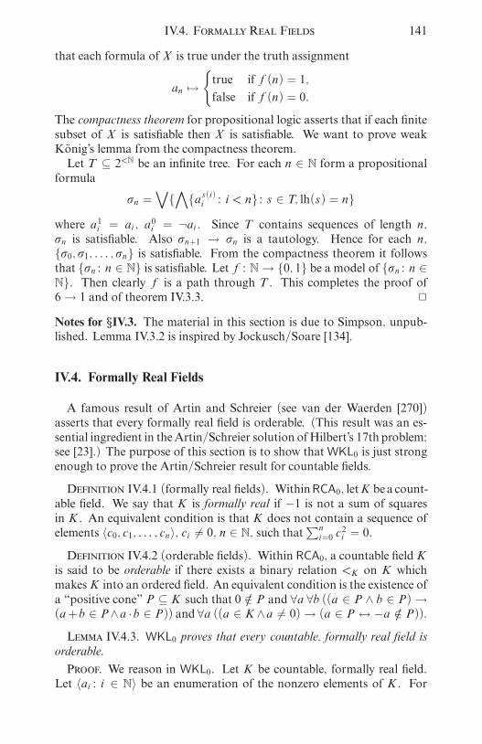
i

i

i

i

i

i

i

i

IV.4. Formally Real Fields 141

that each formula of X is true under the truth assignment

an 7→true if f(n) = 1,

false if f(n) = 0.

The compactness theorem for propositional logic asserts that if each finitesubset of X is satisfiable then X is satisfiable. We want to prove weakKonig’s lemma from the compactness theorem.Let T ⊆ 2<N be an infinite tree. For each n ∈ N form a propositionalformula

ón =∨

∧

as(i)i : i < n : s ∈ T, lh(s) = n

where a1i = ai , a0i = ¬ai . Since T contains sequences of length n,

ón is satisfiable. Also ón+1 → ón is a tautology. Hence for each n,ó0, ó1, . . . , ón is satisfiable. From the compactness theorem it followsthat ón : n ∈ N is satisfiable. Let f : N → 0, 1 be a model of ón : n ∈N. Then clearly f is a path through T . This completes the proof of6→ 1 and of theorem IV.3.3. 2

Notes for §IV.3. The material in this section is due to Simpson, unpub-lished. Lemma IV.3.2 is inspired by Jockusch/Soare [134].

IV.4. Formally Real Fields

A famous result of Artin and Schreier (see van der Waerden [270])asserts that every formally real field is orderable. (This result was an es-sential ingredient in theArtin/Schreier solution ofHilbert’s 17th problem;see [23].) The purpose of this section is to show thatWKL0 is just strongenough to prove the Artin/Schreier result for countable fields.

Definition IV.4.1 (formally real fields). WithinRCA0, letK bea count-able field. We say that K is formally real if −1 is not a sum of squaresin K . An equivalent condition is that K does not contain a sequence ofelements 〈c0, c1, . . . , cn〉, ci 6= 0, n ∈ N, such that

∑ni=0 c

2i = 0.

Definition IV.4.2 (orderable fields). Within RCA0, a countable fieldKis said to be orderable if there exists a binary relation <K on K whichmakesK into an ordered field. An equivalent condition is the existence ofa “positive cone” P ⊆ K such that 0 /∈ P and ∀a ∀b ((a ∈ P ∧ b ∈ P)→(a+b ∈ P∧a ·b ∈ P)) and ∀a ((a ∈ K ∧a 6= 0)→ (a ∈ P ↔ −a /∈ P)).Lemma IV.4.3. WKL0 proves that every countable, formally real field isorderable.

Proof. We reason in WKL0. Let K be countable, formally real field.Let 〈ai : i ∈ N〉 be an enumeration of the nonzero elements of K . For

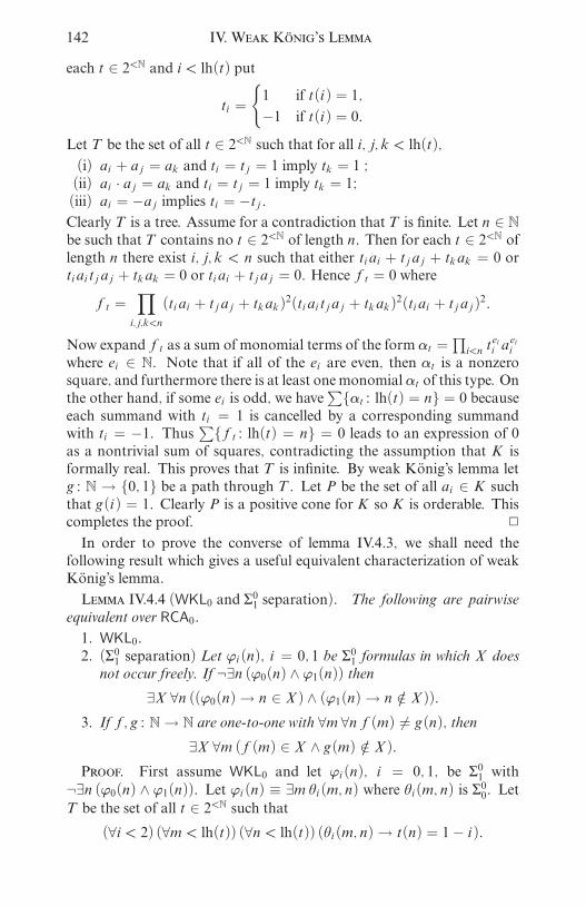
i

i

i

i

i

i

i

i


each t ∈ 2<N and i < lh(t) put

ti =

1 if t(i) = 1,

−1 if t(i) = 0.Let T be the set of all t ∈ 2<N such that for all i, j, k < lh(t),

(i) ai + aj = ak and ti = tj = 1 imply tk = 1 ;(ii) ai · aj = ak and ti = tj = 1 imply tk = 1;(iii) ai = −aj implies ti = −tj .Clearly T is a tree. Assume for a contradiction that T is finite. Let n ∈ Nbe such that T contains no t ∈ 2<N of length n. Then for each t ∈ 2<N oflength n there exist i, j, k < n such that either tiai + tjaj + tkak = 0 ortiai tjaj + tkak = 0 or tiai + tjaj = 0. Hence ft = 0 where

ft =∏

i,j,k<n

(tiai + tjaj + tkak)2(tiai tjaj + tkak)

2(tiai + tjaj)2.

Now expandft as a sum of monomial terms of the form αt =∏i<n t

eii aeii

where ei ∈ N. Note that if all of the ei are even, then αt is a nonzerosquare, and furthermore there is at least onemonomial αt of this type. Onthe other hand, if some ei is odd, we have

∑αt : lh(t) = n = 0 becauseeach summand with ti = 1 is cancelled by a corresponding summandwith ti = −1. Thus ∑ft : lh(t) = n = 0 leads to an expression of 0as a nontrivial sum of squares, contradicting the assumption that K isformally real. This proves that T is infinite. By weak Konig’s lemma letg : N → 0, 1 be a path through T . Let P be the set of all ai ∈ K suchthat g(i) = 1. Clearly P is a positive cone for K so K is orderable. Thiscompletes the proof. 2

In order to prove the converse of lemma IV.4.3, we shall need thefollowing result which gives a useful equivalent characterization of weakKonig’s lemma.

Lemma IV.4.4 (WKL0 and Σ01 separation). The following are pairwiseequivalent over RCA0.

1. WKL0.2. (Σ01 separation) Let ϕi(n), i = 0, 1 be Σ

01 formulas in which X does

not occur freely. If ¬∃n (ϕ0(n) ∧ ϕ1(n)) then∃X ∀n ((ϕ0(n)→ n ∈ X ) ∧ (ϕ1(n)→ n /∈ X )).

3. If f, g : N → N are one-to-one with ∀m ∀n f(m) 6= g(n), then∃X ∀m (f(m) ∈ X ∧ g(m) /∈ X ).

Proof. First assume WKL0 and let ϕi(n), i = 0, 1, be Σ01 with

¬∃n (ϕ0(n) ∧ ϕ1(n)). Let ϕi (n) ≡ ∃m èi(m, n) where èi(m, n) is Σ00. LetT be the set of all t ∈ 2<N such that

(∀i < 2) (∀m < lh(t)) (∀n < lh(t)) (èi(m, n)→ t(n) = 1− i).

i

i

i

i

i

i

i

i

IV.4. Formally Real Fields 143

T exists by Σ00 comprehension. Clearly T is an infinite tree. By weakKonig’s lemma let X be a set whose characteristic function is a paththrough T . Then clearly X satisfies the conclusion of 2. This proves that1 implies 2. The equivalence of 2 and 3 is immediate from lemma II.3.7.It remains to prove that 2 implies 1. Assume 2 and let T ⊆ 2<N be an

infinite tree. Let è(n, ó) be the Σ00 formula ∃ô (lh(ô) = n ∧ ô ∈ T ∧ ô ⊇ó). Let ϕ(ó, i) be the Σ01 formula ∃n (è(n, óa〈i〉) ∧ ¬è(n, óa〈1 − i〉)).Clearly ¬∃ó (ϕ(ó, 0) ∧ ϕ(ó, 1)) so by the assumption 2 let X be such that∀ó ((ϕ(ó, 0) → ó ∈ X ) ∧ (ϕ(ó, 1) → ó /∈ X )). Now define a sequenceof sequences ó0 ⊆ ó1 ⊆ · · · ⊆ ók ⊆ · · · in 2<N by ó0 = empty sequence,ók+1 = ók

a〈0〉 if ók ∈ X , ók+1 = óka〈1〉 if ók /∈ X . Clearly lh(ók) = kfor all k. We claim that è(n, ók) holds for all k and n with k ≤ n. Fix n.We prove the claim by induction on k ≤ n. Trivially è(n, ó0) since T isinfinite. Assume inductively that è(n, ók) holds for some k < n. Clearlyeither è(n, ók

a〈0〉) or è(n, óka〈1〉) must hold. If ¬è(óka〈0〉) then wehave ϕ(ók , 1), hence ók /∈ X so ók+1 = óka〈1〉 whence è(n, ók+1). If¬è(óka〈1〉) then we have ϕ(ók , 0), hence ók ∈ X so ók+1 = óka〈0〉whence è(n, ók+1). In any case è(n, ók+1) holds so our claim is proved. Inparticular we have è(n, ón), i.e., ón ∈ T , for all n. so f =

⋃ón : n ∈ Nis a path through T . This proves weak Konig’s lemma from 2. The proofof lemma IV.4.4 is complete. 2

We now show that weak Konig’s lemma is needed to prove the order-ability of countable, formally real fields.


1. WKL0.2. Every countable, formally real field is orderable.3. Every countable, formally real field has a real closure.

Proof. Assertions 2 and 3 are equivalent in view of theorem II.9.7.Lemma IV.4.3 shows that 1 implies 2. It remains to prove that 2 implies1. Assume 2. Instead of proving weak Konig’s lemma directly, we shallprove the equivalent statement IV.4.4.3. Let f, g : N → N be functionssuch that ∀i ∀j f(i) 6= g(j). Let 〈pk : k ∈ N〉 be an enumeration of therational primes, p0 = 2, p1 = 3, p2 = 5, . . . . By theorem II.9.7 let Qbe the real closure of the rational field Q. For each n ∈ N let Kn be thesubfield of Q(

√−1) generated by

4√pf(i) : i < n ∪

√−√pg(j) : j < n

∪ √pk : k < n.

Because we lack Σ01 comprehension we cannot form the subfield⋃n∈NKn.

However, we can apply lemma II.3.7 to find a field K and an embeddingh : K → Q(

√−1) such that ∀b (∃n (b ∈ Kn)↔ ∃a (h(a) = b)).

i

i

i

i

i

i

i

i


Note that each Kn is embeddable into Q by taking √pf(i) to √pf(i)

and√pk to−

√pk whenever k 6= f(i) for all i < n. SinceQ is an ordered

field, it follows that each Kn is formally real. Hence K is formally real.Hence by 2, K is orderable. Fix an ordering of K . Since h−1

√pf(i) has

a square root in K (namely h−1 4√pf(i)), we must have h

−1√pf(i) > 0.On the other hand, since −h−1√pg(j) has a square root in K (namelyh−1

√−√pg(j)), we must have h

−1√pg(j) < 0. By ∆01 comprehension letX be the set of all k ∈ N such that h−1

√pk > 0. Then ∀i (f(i) ∈ X )

and ∀j (g(j) /∈ X ). By lemma IV.4.4 this gives weak Konig’s lemma. Theproof of the theorem is complete. 2

Remark IV.4.6. WKL0 is also equivalent over RCA0 to the assertionthat every countable torsion-free Abelian group is orderable. This resultof Hatzikiriakou/Simpson [113] is related to a recursive counterexampleof Downey/Kurtz [47]. Solomon [251] has obtained additional ReverseMathematics results concerning orderability of countable groups.

Remark IV.4.7. WKL0 is also equivalent over RCA0 to the theorem onextension of valuations for countable fields: Given a monomorphism ofcountable fields h : K1 → K2 and a valuation ring V1 of K1, there existsa valuation ring V2 of K2 such that V1 = h−1(V2). This result is due toHatzikiriakou/Simpson [112].

Exercise IV.4.8. Show that RCA0 proves Π01 separation: For any Π01

formulasø1(n) andø0(n) in whichZ does not occur freely, ¬∃n (ø1(n)∧ø0(n)) → ∃Z ∀n ((ø1(n) → n ∈ Z) ∧ (ø0(n) → n /∈ Z)). This is incontrast to lemma IV.4.4.

Notes for §IV.4. Themain results of this section are fromFriedman/Simp-son/Smith [78]. A corollary of theorem IV.4.5 is that there exists a re-cursive, formally real field with no recursive ordering. This result isoriginally due to Ershov [54]. An improvement of Ershov’s result due toMetakides/Nerode [187] states that for any recursive tree T ⊆ 2<N thereexists a recursive, formally real fieldK such that the space of all orderingsof K is recursively homeomorphic to [T ], the closed set in 2N consistingof all paths through T .

IV.5. Uniqueness of Algebraic Closure

In §II.9 we showed that RCA0 proves that every countable field has analgebraic closure. In this section we show thatWKL0 is needed to provethat these algebraic closures are unique.

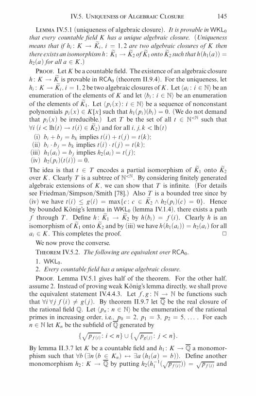
i

i

i

i

i

i

i

i

IV.5. Uniqueness of Algebraic Closure 145

Lemma IV.5.1 (uniqueness of algebraic closure). It is provable inWKL0

that every countable field K has a unique algebraic closure. (Uniqueness

means that if hi : K → Ki , i = 1, 2 are two algebraic closures of K then

there exists an isomorphism h : K1 → K2 of K1 onto K2 such that h(h1(a)) =h2(a) for all a ∈ K .)Proof. LetK be a countable field. The existence of an algebraic closureh : K → K is provable in RCA0 (theorem II.9.4). For the uniqueness, let

hi : K → Ki , i = 1, 2 be two algebraic closures ofK . Let 〈ai : i ∈ N〉 be anenumeration of the elements of K and let 〈bi : i ∈ N〉 be an enumerationof the elements of K1. Let 〈pi(x) : i ∈ N〉 be a sequence of nonconstantpolynomials pi(x) ∈ K [x] such that h1(pi)(bi) = 0. (We do not demandthat pi(x) be irreducible.) Let T be the set of all t ∈ N<N such that

∀i (i < lh(t)→ t(i) ∈ K2) and for all i, j, k < lh(t)(i) bi + bj = bk implies t(i) + t(j) = t(k);(ii) bi · bj = bk implies t(i) · t(j) = t(k);(iii) h1(ai) = bj implies h2(ai) = t(j);(iv) h2(pi)(t(i)) = 0.

The idea is that t ∈ T encodes a partial isomorphism of K1 onto K2over K . Clearly T is a subtree of N<N. By considering finitely generatedalgebraic extensions of K , we can show that T is infinite. (For detailssee Friedman/Simpson/Smith [78].) Also T is a bounded tree since by

(iv) we have t(i) ≤ g(i) = maxc : c ∈ K2 ∧ h2(pi)(c) = 0. Henceby bounded Konig’s lemma in WKL0 (lemma IV.1.4), there exists a pathf through T . Define h : K1 → K2 by h(bi) = f(i). Clearly h is an

isomorphism of K1 onto K2 and by (iii) we have h(h1(ai)) = h2(ai) for allai ∈ K . This completes the proof. 2

We now prove the converse.

Theorem IV.5.2. The following are equivalent over RCA0.

1. WKL0.2. Every countable field has a unique algebraic closure.

Proof. Lemma IV.5.1 gives half of the theorem. For the other half,assume 2. Instead of proving weak Konig’s lemma directly, we shall provethe equivalent statement IV.4.4.3. Let f, g : N → N be functions suchthat ∀i ∀j f(i) 6= g(j). By theorem II.9.7 let Q be the real closure ofthe rational field Q. Let 〈pn : n ∈ N〉 be the enumeration of the rationalprimes in increasing order, i.e., p0 = 2, p1 = 3, p2 = 5, . . . . For eachn ∈ N let Kn be the subfield of Q generated by

√pf(i) : i < n ∪ √pg(j) : j < n.By lemma II.3.7 let K be a countable field and h1 : K → Q a monomor-phism such that ∀b (∃n (b ∈ Kn) ↔ ∃a (h1(a) = b)). Define anothermonomorphism h2 : K → Q by putting h2(h−11 (

√pf(i))) =

√pf(i) and

i

i

i

i

i

i

i

i


h2(h−11 (

√pg(j))) = −√

pg(j). Thus h1, h2 : K → Q(√−1) are two alge-

braic closures of K . By 2 there exists an automorphism h : Q(√−1) →

Q(√−1) such that h(h1(a)) = h2(a) for all a ∈ K . Let X be the set of all

m such that h(√pm) =

√pm. Then

h(√pf(i)) = h(h1(h

−11 (pf(i)))) = h2(h

−11 (√pf(i))) =

√pf(i)

and

h(√pg(j)) = h(h1(h

−11 (pg(j)))) = h2(h

−11 (√pg(j))) = −√pg(j)

so f(i) ∈ X and g(j) /∈ X . By lemma IV.4.4 this implies weak Konig’slemma. The proof of the theorem is complete. 2

Notes for §IV.5. The results of this section are from Friedman/Simpson/Smith [78].

IV.6. Prime Ideals in Countable Commutative Rings

In this sectionwe show thatWKL0 is just strong enough to accommodatethe development of an important topic in commutative algebra.

Definition IV.6.1 (prime ideals). Within RCA0, let R be a countablecommutative ring. A prime ideal of R is a set P ⊆ R such that P is anideal of R (definition III.5.2) and ∀a ∀b (a · b ∈ P → (a ∈ P ∨ b ∈ P)).A basic theoremof commutative algebra asserts that every commutativering has a prime ideal. The usual way to prove this theorem is to obtain amaximal ideal (by Zorn’s lemma) and then to observe that maximal idealsare prime. This method cannot work in WKL0 since by theorem III.5.5the existence of maximal ideals is not provable inWKL0. Nevertheless, wehave:

Lemma IV.6.2 (existence of prime ideals). It is provable in WKL0 thatevery countable commutative ring possesses a prime ideal.

Proof. We reason in WKL0. Let R be a countable commutative ringand let 〈ai : i ∈ N〉 be an enumeration of the elements ofR. Use primitiverecursion (theorem II.3.4) to define a sequence of (codes for) finite setsXs ⊆ R, s ∈ 2<N, beginning with X〈〉 = 0. (Here 〈〉 denotes the emptysequence.) Let s ∈ 2<N be given and suppose that Xs has already beendefined. Let

lh(s) = 4 · ((i, j), m) + k, 0 ≤ k < 4, (11)

where (i, j) denotes the pairing function (theorem II.2.2).Case 1: k = 0. If ai · aj ∈ Xs put Xsa〈0〉 = Xs ∪ ai and Xsa〈1〉 =Xs ∪ aj; otherwise put Xsa〈0〉 = Xs and Xsa〈1〉 = ∅ = the empty set.

i

i

i

i

i

i

i

i

IV.6. Prime Ideals in Countable Commutative Rings 147

Case 2: k = 1. Put Xsa〈0〉 = ∅. If ai ∈ Xs and aj ∈ Xs putXsa〈1〉 = Xs ∪ ai + aj, otherwise Xsa〈1〉 = Xs .Case 3: k = 2. Put Xsa〈0〉 = ∅. If ai ∈ Xs put Xsa〈1〉 = Xs ∪ ai · aj,otherwise Xsa〈1〉 = Xs .Case 4: k = 3. Put Xsa〈0〉 = ∅. If 1 ∈ Xs put Xsa〈1〉 = ∅, otherwiseXsa〈1〉 = Xs .If lh(s) is not as in (11), put Xsa〈0〉 = ∅ and Xsa〈1〉 = Xs . This

completes the construction of Xs for all s ∈ 2<N.Let S be the set of all s ∈ 2<N such that Xs 6= ∅. Clearly S is a tree.We claim that for each n ∈ N there exists s ∈ S of length n such thatXs does not generate R as an R-module. For n = 0 the claim is trivial.If n ≡ 1, 2, or 3 mod 4 and the claim holds for n then trivially it holdsfor n + 1. Suppose n ≡ 0 mod 4 and the claim holds for n. Let s ∈ Sbe of length n such that Xs does not generate R as an R-module. Letn = 4 · ((i, j), m). If ai · aj /∈ Xs then trivially our claim holds for n + 1.If ai · aj ∈ Xs then we make a subclaim that Xsa〈0〉 = Xs ∪ ai andXsa〈1〉 = Xs ∪ aj do not both generate R as an R-module. If theydid, we would have 1 = c + rai = d + saj where r, s ∈ R and c, dare finite linear combinations of elements of Xs with coefficients from R.Then 1 = cd + csaj + drai + rsaiaj so Xs generates R as a R-module, acontradiction. This proves the subclaim. Hence our claim holds for n+1.The claim for all n ∈ N now follows by Π01 induction on n.The above claim implies that S is infinite. Hence by weak Konig’slemma S has a path, call it f. If it were now possible to form the set ofall a ∈ R such that ∃n (a ∈ Xf[n]), then clearly this set would be a primeideal of R and the proof of lemma IV.6.2 would be complete. (Here f[n]denotes the initial sequence of f of length n.) Unfortunately, we cannotform this set because we lack Σ01 comprehension. However, we can usebounded Σ01 comprehension to finish the proof as follows.We may safely assume that our enumeration 〈ai : i ∈ N〉 of R is suchthat a0 = 0 and a1 = 1. Let T be the set of all t ∈ 2<N such that

(i) 0 < lh(t) implies t(0) = 0;(ii) 1 < lh(t) implies t(1) = 1;(iii) if i, j, k < lh(t) then

(a) t(i) = t(j) = 0 and ai + aj = ak imply t(k) = 0;(b) t(i) = 0 and ai · aj = ak imply t(k) = 0;(c) t(i) = t(j) = 1 and ai · aj = ak imply t(k) = 1.

Clearly T is a tree. We claim that T is infinite. To see this, let m ∈ Nbe given. By bounded Σ01 comprehension (theorem II.3.9) let Y be theset of all i < m such that ∃n (ai ∈ Xf[n]). Define t ∈ 2<N, lh(t) = m byputting t(i) = 0 if i ∈ Y , t(i) = 1 if i /∈ Y . Then clearly t ∈ T andlh(t) = m. This proves that T is infinite. Hence by another application

i

i

i

i

i

i

i

i


of weak Konig’s lemma there exists a path g through T . Let P be the setof all ai ∈ R such that g(i) = 0. Then clearly P is a prime ideal of R.This completes the proof of lemma IV.6.2. 2

We now turn to the reversal. First, a definition:

Definition IV.6.3 (radical ideals). Within RCA0, let R be a countablecommutative ring. A radical ideal of R is an ideal J ⊆ R (cf. definitionIII.5.2) such that an ∈ J implies a ∈ J for all a ∈ R, n ∈ N.

Clearly every prime ideal of R is a radical ideal of R.

Theorem IV.6.4 (reversal). The following assertions are pairwise equiv-alent over RCA0.

1. WKL0.2. Every countable commutative ring contains a prime ideal.3. Every countable commutative ring contains a radical ideal.

Proof. The implication from 1 to 2 has already been proved as lemmaIV.6.2. The implication from 2 to 3 is trivial. It remains to prove that3 implies 1. We reason in RCA0. Assume 3. Instead of proving weakKonig’s lemma directly, we shall prove the equivalent IV.4.4.3.Let f, g : N → N be given with ∀i ∀j (f(i) 6= g(j)). Let R0 = Q[〈xn :n ∈ N〉] be the polynomial ring over rational field Q with countably manyindeterminates xn, n ∈ N. Let I ⊆ R0 be the ideal generated by thepolynomials xm+1

f(m)and xm+1

g(m)− 1, m ∈ N. To see that I exists, note that

any givenf ∈ R0 can be put into a normal formf∗ ≡ f modulo I , whereif xkn occurs in f

∗ then n 6= f(m), g(m) for all m < k. Thus f ∈ I ifand only if f∗ = 0, so I exists by ∆01 comprehension. Form the quotientring R = R0/I . By our assumption 3, let J be a radical ideal in R. LetJ0 be the ideal in R0 which corresponds to J . Then J0 is a radical ideal inR0 and I ⊆ J0. It follows that xf(m) ∈ J0 and xg(m) /∈ J0 for all m ∈ N.Setting X = n : xn ∈ J0 we obtain ∀m (f(m) ∈ X ∧ g(m) /∈ X ). Thusby IV.4.4 we have weak Konig’s lemma. This completes the proof. 2

Corollary IV.6.5. RCA0 is not strong enough to prove that every count-able commutative ring has a prime (or even radical) ideal.

Proof. Immediate from theorem IV.6.4 and the fact (to be proved in§VIII.2) that the theorems of RCA0 are strictly included in those ofWKL0.

2

Exercise IV.6.6. Show that the following is provable in WKL0. Let Rbe a countable commutative ring. Let ϕ(a) and ø(a) be Σ01 such that

1. ∀a ∀b ((ϕ(a) ∧ ø(b))→ (a ∈ R ∧ b ∈ R ∧ a 6= b)),2. ϕ(0) ∧ ø(1),3. ∀a ∀b ((ϕ(a) ∧ ϕ(b))→ ϕ(a + b)),4. ∀a ∀r ((ϕ(a) ∧ r ∈ R)→ ϕ(r · a)),5. ∀a ∀b ((ø(a) ∧ ø(b))→ ø(a · b)).

i

i

i

i

i

i

i

i

IV.7. Fixed Point Theorems 149

ThenR has a prime idealP such that∀a (ϕ(a)→ a ∈ P) and∀a (ø(a)→a /∈ P).

Notes for §IV.6. Themain results in this section are fromFriedman/Simp-son/Smith [78, 79].

IV.7. Fixed Point Theorems

In this and the next two sections, we resume the study of analysis inWKL0, which was begun in §§IV.1 and IV.2.A famous theorem of Brouwer states that any continuous mapping ofa k-simplex into itself has a fixed point. The purpose of this section is toshow thatBrouwer’s theoremand its generalization to infinite-dimensionalspaces are provable inWKL0. We shall also obtain a reversal showing thatBrouwer’s theorem is equivalent to weak Konig’s lemma over RCA0.We begin by presenting one of the well known proofs of Brouwer’stheorem, withinWKL0. We use the proof via Sperner’s lemma.

Definition IV.7.1 (k-simplices). The following definitions are made inRCA0. For k ∈ N, a k-simplex S is the convex hull of k + 1 affinelyindependent points s0, . . . , sk in Rn, called the vertices of S. We cancoordinatize S by identifying each point x ∈ S with the unique (k+1)-tuple (x0, . . . , xk) such that x =

∑ki=0 xisi ,

∑ki=0 xi = 1, and xi ≥ 0 for

all i ≤ k. Clearly S is a compact metric space.If S is a simplex, a face of S is any simplex whose vertices are a subsetof the vertices of S. For any point x ∈ S, the carrier of x is the smallestface of S which contains x.

Definition IV.7.2 (simplicial subdivision). Within RCA0, let S be ak-simplex. A simplicial subdivision of S is a finite set of k-simplicesS0, . . . , Sm such that S = S0 ∪ · · · ∪ Sm and, for all i < j ≤ m, Si ∩ Sj iseither empty or a common face of Si and Sj .

Definition IV.7.3 (admissible labeling). Within RCA0, let S be a k-simplex, and let P be a finite set of points in S which includes the verticesof S. An admissible labeling ofP is a mapping fromP into 0, . . . , k suchthat (i) the vertices of S are mapped to the full set of labels 0, . . . , k;and (ii) for every x ∈ P, the label of x is the same as the label of one ofthe vertices of the carrier of x.

Lemma IV.7.4 (Sperner’s lemma). The following is provable in RCA0.Let S be a k-simplex, k ∈ N, and let S0, . . . , Sm be a simplicial subdi-vision of S. Suppose that the vertices of S0, . . . , Sm are admissibly labeled.Then for some i ≤ m, the vertices of Si are mapped to the full set of labels0, . . . , k.

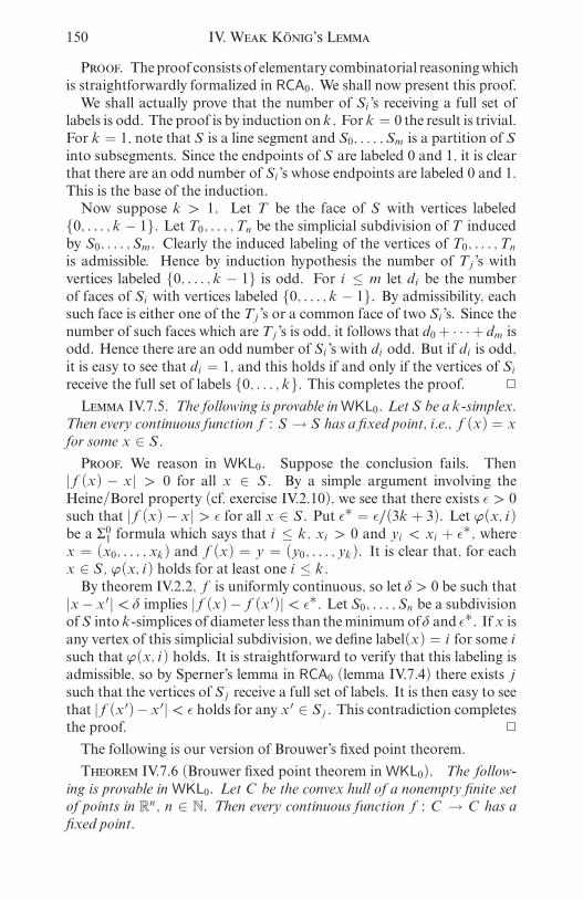
i

i

i

i

i

i

i

i


Proof. Theproof consists of elementary combinatorial reasoningwhichis straightforwardly formalized in RCA0. We shall now present this proof.We shall actually prove that the number of Si ’s receiving a full set oflabels is odd. The proof is by induction on k. For k = 0 the result is trivial.For k = 1, note that S is a line segment and S0, . . . , Sm is a partition of Sinto subsegments. Since the endpoints of S are labeled 0 and 1, it is clearthat there are an odd number of Si ’s whose endpoints are labeled 0 and 1.This is the base of the induction.Now suppose k > 1. Let T be the face of S with vertices labeled

0, . . . , k − 1. Let T0, . . . , Tn be the simplicial subdivision of T inducedby S0, . . . , Sm . Clearly the induced labeling of the vertices of T0, . . . , Tnis admissible. Hence by induction hypothesis the number of Tj ’s withvertices labeled 0, . . . , k − 1 is odd. For i ≤ m let di be the numberof faces of Si with vertices labeled 0, . . . , k − 1. By admissibility, eachsuch face is either one of the Tj ’s or a common face of two Si ’s. Since thenumber of such faces which are Tj ’s is odd, it follows that d0+ · · ·+ dm isodd. Hence there are an odd number of Si ’s with di odd. But if di is odd,it is easy to see that di = 1, and this holds if and only if the vertices of Sireceive the full set of labels 0, . . . , k. This completes the proof. 2

Lemma IV.7.5. The following is provable inWKL0. Let S be a k-simplex.Then every continuous functionf : S → S has a fixed point, i.e., f(x) = xfor some x ∈ S.Proof. We reason in WKL0. Suppose the conclusion fails. Then

|f(x) − x| > 0 for all x ∈ S. By a simple argument involving theHeine/Borel property (cf. exercise IV.2.10), we see that there exists ǫ > 0such that |f(x)− x| > ǫ for all x ∈ S. Put ǫ∗ = ǫ/(3k + 3). Let ϕ(x, i)be a Σ01 formula which says that i ≤ k, xi > 0 and yi < xi + ǫ

∗, wherex = (x0, . . . , xk) and f(x) = y = (y0, . . . , yk). It is clear that, for eachx ∈ S, ϕ(x, i) holds for at least one i ≤ k.By theorem IV.2.2, f is uniformly continuous, so let ä > 0 be such that

|x− x′| < ä implies |f(x)−f(x′)| < ǫ∗. Let S0, . . . , Sn be a subdivision

ofS into k-simplices of diameter less than theminimum of ä and ǫ∗. If x is

any vertex of this simplicial subdivision, we define label(x) = i for some isuch that ϕ(x, i) holds. It is straightforward to verify that this labeling isadmissible, so by Sperner’s lemma in RCA0 (lemma IV.7.4) there exists jsuch that the vertices of Sj receive a full set of labels. It is then easy to seethat |f(x′)− x′| < ǫ holds for any x′ ∈ Sj . This contradiction completesthe proof. 2

The following is our version of Brouwer’s fixed point theorem.

Theorem IV.7.6 (Brouwer fixed point theorem inWKL0). The follow-ing is provable inWKL0. Let C be the convex hull of a nonempty finite setof points in Rn, n ∈ N. Then every continuous function f : C → C has afixed point.

i

i

i

i

i

i

i

i


Proof. Let k be the dimension of C . We can find a k-simplex S in Rn

such that C ⊆ S. Using elementary linear algebra in RCA0 (cf. exerciseII.4.11), we can show that C is a retract of S, i.e., there is a continuousfunction r : S → C such that r(x) = x for all x ∈ C . Given a continuousfunction f : C → C , consider g : S → C given by g(x) = f(r(x)). Bytheorem IV.7.5, let x ∈ S be such that g(x) = x. Then x ∈ C , hencer(x) = x, hence f(x) = g(x) = x. This completes the proof. 2

We shall now obtain a reversal showing that weak Konig’s lemma isneeded to prove Brouwer’s theorem, even for the unit square.

Theorem IV.7.7 (reversal). The following are pairwise equivalent overRCA0.

1. Let C be the convex hull of a nonempty finite set of points in Rn,n ∈ N. Then every continuous function f : C → C has a fixed point.

2. LetC be the unit square, [0, 1]× [0, 1]. Then every continuous functionf : C → C has a fixed point.

3. Weak Konig’s lemma.

Proof. The implication 1 → 2 is trivial, and 3 → 1 has already beenproved as theorem IV.7.6. It remains to prove 2 → 3. Working withinRCA0, assume that weak Konig’s lemma is false. Let T ⊆ 2<N be aninfinite tree with no infinite path. We shall useT to construct a continuousfunction f : C → C with no fixed point, where C = [0, 1]× [0, 1].Let ∂C be the boundary of C , i.e., the four edges of the unit square. It

suffices to show that ∂C is a retract of C . For, once we have a retractionmap r : C → ∂C , we can let f : C → ∂C consist of r followed by a 90orotation of ∂C . Clearly such an f has no fixed point.We claim that there exists a singular covering of [0, 1], i.e., a coveringof [0, 1] by an infinite sequence of closed rational intervals In = [an , bn],an, bn ∈ Q, an < bn, n ∈ N, such that for all m 6= n, Im ∩ In consistsof at most one point. To see this, define intervals [có , dó ], ó ∈ 2<N, byputting c〈〉 = 0, d〈〉 = 1, cóa〈0〉 = có , cóa〈1〉 = dóa〈0〉 = (có + dó)/2,

and dóa〈1〉 = dó . Let 〈ón : n ∈ N〉 be an enumeration of T = ó ∈2<N : ó /∈ T ∧ ó[lh(ó) − 1] ∈ T, and put In = [an, bn] = [cón , dón ].Clearly 〈In : n ∈ N〉 has the desired properties, so our claim is proved.For each n ∈ N, put

An =

⋃

m≤n

Im × In

∪

⋃

m≤n

In × Im

and

Bn = ([0, 1]× In) ∪ (In × [0, 1]).

Note that C =⋃n∈NAn . Note also that An is properly included in Bn .

i

i

i

i

i

i

i

i


Our retraction map r : C → ∂C will be defined in stages. We begin bydefining r on ∂C to be the identity map. At stage n, we assume that rhas already been defined on ∂C and on Am for all m < n, and we definer on An . Let Pn0, . . . , Pnkn be the connected components of An . Since Anis properly included in Bn , it follows that ∂Pni has at least one edge eniwhich, except for its endpoints, lies inside Bn \ ∂C , hence is disjoint from⋃m<n Am. Let e

′ni be eni minus its endpoints. We define r on Pni to consist

of a continuous retraction ofPni onto ∂Pni \ e′ni , followed by a continuousmapping of ∂Pni \ e′i into ∂C which is compatible with the part of r thathas already been defined. This defines r on An =

⋃i≤knPni .

It can be shown that the above construction gives rise to a continuousfunction r defined on all of C =

⋃n∈NAn . Clearly r is a retraction of C

onto ∂C . This completes the proof. 2

Weshall nowobtain an infinite-dimensional generalization ofBrouwer’stheorem, within WKL0. The theorem which we shall prove is closelyrelated to the Schauder/Tychonoff fixed point theorem. First, we needthe following technical lemma.

Lemma IV.7.8. The following is provable in WKL0. Let C be a closedset in a compact metric space X . Given ǫ > 0, there exists a finite set ofpoints c1, . . . , cm ∈ C such that for all x ∈ C , d (x, ci) < ǫ for some i ,1 ≤ i ≤ m.Proof. By compactness, there exists a finite set of pointsx1, . . . , xn ∈ Xsuch that for all x ∈ X there exists i such that d (x, xi ) < ǫ/2. By theoremIV.1.7, we see that the formula

ϕ(i) ≡ ∃x (x ∈ C and d (x, xi) ≤ ǫ/2)

is equivalent to a Π01 formula. By bounded Π01 comprehension, let I ⊆

1, . . . , n be the set of i such that ϕ(i) holds. By theorem IV.1.8, let〈ci : i ∈ I 〉 be a sequence of points such that ci ∈ C and d (ci , xi) ≤ ǫ/2.Then for all x ∈ C we have d (x, xi) < ǫ/2 for some i , hence i ∈ I , henced (ci , xi ) ≤ ǫ/2, hence d (x, ci) < ǫ. We can renumber the ci ’s as c1, . . . , cmwhere m = |I | ≤ n. This completes the proof. 2

The following is our version of the Schauder/Tychonoff fixed pointtheorem. Recall from examples II.5.5 and III.2.6 that the Hilbert cube[0, 1]N is compact.

Theorem IV.7.9 (Schauder fixed point theorem inWKL0). The follow-ing is provable inWKL0. Let C be a nonempty closed convex set in [−1, 1]N.Then every continuous function f : C → C has a fixed point.Proof. Suppose not. Let f : C → C be continuous such that f(x) 6=x for all x ∈ C . For m ≥ 1 and x = 〈xi : i ∈ N〉 ∈ RN, we put‖x‖m = maxi<m |xi |. Let us write Bm(x, ǫ) (respectively B∗m(x, ǫ)) forthe open (respectively closed) ball consisting of all y ∈ RN such that‖y − x‖m < ǫ (respectively ‖y − x‖m ≤ ǫ). By the Heine/Borel covering

i

i

i

i

i

i

i

i


principle in WKL0 (theorem IV.1.5), there exist m ∈ N and ǫ > 0 suchthat f(x) /∈ Bm(x, ǫ) for all x ∈ C . We shall obtain a contradiction byfinding a point x ∈ C such that f(x) ∈ Bm(x, ǫ).By the previous lemma, let c0, . . . , ck ∈ C be such that C is coveredby the open sets Ui = Bm(ci , ǫ), i ≤ k. Let D ⊆ C be the convex hullof c0, . . . , ck . Recall from example II.5.5 that RN = A where A is the setof eventually 0 sequences of rational numbers. Let ϕ(k, a, r, i) be a Σ01formula which says that n ∈ N, a ∈ A, r ∈ Q+, i ≤ k, and

B∗n (a, r) ⊆ (RN \C ) ∪ f−1(Ui).

It is straightforward to show thatRN is covered by open sets Bn(a, r) suchthatϕ(k, a, r, i) holds for some i ≤ k. Hence by theHeine/Borel principlethere exists a covering of C by finitely many open sets Bnij (aij , rij), i ≤ k,j < li , with ϕ(kij , aij , rij , i). Put Vi =

⋃j<liBnij (aij , rij). Thus C is

covered by the open sets Vi , i ≤ k, and f(Vi) ⊆ Ui . Put

n = maxm ∪ nij : i ≤ k, j < li.

For any x = 〈xi : i ∈ N〉 ∈ RN, let us write x = 〈xi : i < n〉 ∈ Rn. LetD be the convex hull of c0, . . . , ck inRk , and letV i =

⋃j<liBnij (aij , rij) ⊆

Rn. Thus D is covered by open sets V i , i ≤ k, in Rn. As in the proofof theorem II.7.2, let gi : D → [0, 1], i ≤ k, be a sequence of continuousfunctions such that

∑ki=0 gi(x) = 1 for all x ∈ D, and gi(x) > 0 implies

x ∈ V i . Define g : D → D by g(x) =∑ki=0 gi(x)c i .By theorem IV.7.6, there is x′ ∈ D such that g(x ′) = x′. Put

x′ =k∑

i=0

gi(x′)ci

and note that x′ ∈ C . By bounded Σ01 comprehension, let I be the set ofall i ≤ k such that gi(x′) > 0. Then for all i ∈ I we have x′ ∈ V i , hencex′ ∈ Vi , hence f(x′) ∈ Ui = Bm(ci , ǫ), i.e., ‖f(x′) − ci‖m < ǫ. Since∑gi (x

′) = 1, it follows that

‖f(x′)− x′‖m =∥∥∥∥∥∑

i∈I

gi(x′)f(x′)−

∑

i∈I

gi(x′)ci

∥∥∥∥∥m

≤∑

i∈I

gi (x′)‖f(x′)− ci‖m < ǫ.

Thus f(x′) ∈ Bm(x′, ǫ) and the proof is complete. 2

Notes for §IV.7. Shioji/Tanaka [219] proved versions of the Brouwer andSchauder fixed point theorems, withinWKL0. Our results in this section

i

i

i

i

i

i

i

i


are variants of those of Shioji/Tanaka [219]. Our proof of Brouwer’s theo-remwithinWKL0 ismodeled after thewell known proof of Brouwer’s theo-remvia Sperner’s lemma (cf. Tompkins [267]). The fact that Brouwer’s the-orem for [0, 1]×[0, 1] implies weakKonig’s lemma is due to Shioji/Tanaka[219], based on a recursive counterexample due to Orevkov [199].

IV.8. Ordinary Differential Equations

In this section we discuss Peano’s existence theorem for solutions ofordinary differential equations. Peano’s theorem says that, if f(x, y) iscontinuous in some neighborhood of (0, 0), then the initial value prob-lem

y′ = f(x, y), y(0) = 0 (12)

has a solution y = φ(x) which is continuously differentiable in someneighborhood of x = 0. Here y′ denotes the derivative of the unknownfunction y = y(x). We shall show that Peano’s theorem is provable inWKL0. We shall also show that Peano’s theorem is equivalent to weakKonig’s lemma over RCA0.We begin by proving Peano’s theorem in WKL0. The proof will bebased on theorem IV.7.9, our WKL0 version of the Schauder fixed pointtheorem.

Theorem IV.8.1 (Peano’s theorem inWKL0). The following is provableinWKL0. Let f(x, y) be a continuous real-valued function on the rectangle−a ≤ x ≤ a, −b ≤ y ≤ b where a, b>0. Then the initial value problem

dy

dx= f(x, y), y(0) = 0

has a continuously differentiable solution y = φ(x) on the interval −α ≤x ≤ α, α = min(a, b/M ), where

M = max|f(x, y)| : − a ≤ x ≤ a,−b ≤ y ≤ b.Proof. We reason inWKL0.Note first thatM exists by theorem IV.2.2.Let A = qi : i ∈ N be an enumeration of the rational numbers in theclosed interval [−α,α]. Thus A = [−α,α]. We may safely assume thatq0 = 0. Let C be the closed convex set in RN consisting of all sequences〈yi : i ∈ N〉 such that y0 = 0 and |yi − yj | ≤M · |qi − qj | for all i, j ∈ N.C is included in the compact product space

∏i∈N[−Mα,Mα] (cf. lemma

III.2.5).To each 〈yi : i ∈ N〉 ∈ C is associated a continuous function

φ : [−α,α]→ R

i

i

i

i

i

i

i

i

IV.8. Ordinary Differential Equations 155

such that φ(qi) = yi for all i ∈ N. Namely, the code Φ of φ is given byputting (qi , r)Φ(b, s) if and only if M · r + |b − yi | < s . Thus we shallidentify points ofC with continuous functions φ : [−α,α]→ R satisfyingφ(0) = 0 and

|φ(x)− φ(x′)| ≤M · |x − x′|for |x|, |x′| ≤ α.We define a continuous function F : C → C as follows. For 〈yi : i ∈

N〉∈C , we put

F (〈yi : i ∈ N〉) =⟨∫ qi

0

f(x, φ(x)) dx : i ∈ N⟩

whereφ : [−α,α]→ R is the continuous function associated to 〈yi : i ∈ N〉as in the previous paragraph. For all i, j ∈ N we have

∣∣∣∣∫ qi

0

f(x, φ(x)) dx −∫ qj

0

f(x, φ(x)) dx

∣∣∣∣ =∣∣∣∣∫ qj

qi

f(x, φ(x)) dx

∣∣∣∣≤M · |qi − qj |

so F (〈yi : i ∈ N〉) ∈ C . Using a modulus of uniform continuity for f (cf.theorem IV.2.2), it is straightforward to construct a code for F .Now by theorem IV.7.9 let 〈yi : i ∈ N〉 ∈ C be a fixed point of F , i.e.,

F (〈yi : i ∈ N〉) = 〈yi : i ∈ N〉.Let φ : [−α,α]→ R be the continuous function associated to 〈yi : i ∈ N〉.Then for all i ∈ N we have

φ(qi) =

∫ qi

0

f(x, φ(x))dx.

It follows easily that

dφ(x)

dx= f(x, φ(x)) and φ(0) = 0

for all x in [−α,α]. This proves our theorem. 2

We remark that it is straightforward to extend the previous theorem soas to apply to initial value problems of the form

y′1 = f1(x, y1, . . . , yn), y1(0) = 0

y′2 = f2(x, y1, . . . , yn), y2(0) = 0

...

y′n = fn(x, y1, . . . , yn), yn(0) = 0

where n ∈ N.We now turn to the reversal of theorem IV.8.1. The following theoremsays that Peano’s theorem is equivalent overRCA0 toweakKonig’s lemma.

i

i

i

i

i

i

i

i


Theorem IV.8.2 (reversal). The following assertions are pairwise equiv-alent over RCA0.

1. WKL0.2. Peano’s theorem, as stated in IV.8.1.3. If f(x, y) is continuous and has a modulus of uniform continuity insome neighborhoodofx = 0, y = 0, then the initial value problem (12)has a continuously differentiable solution y = φ(x) in some intervalcontaining x = 0.

Proof. The implication from 1 to 2 is given by theorem IV.8.1, andthe implication from 2 to 3 is trivial. It remains to prove that 3 implies1. Assume 3. Instead of proving weak Konig’s lemma directly, we shallprove Σ01 separation (lemma IV.4.4.2).Letϕ(n, i) be a Σ01 formula such that¬∃n (ϕ(n, 0)∧ϕ(n, 1)). Working in

RCA0, we shall construct a a continuous functionf(x, y) on the rectangle|x| ≤ 1, |y| ≤ 1, such that |f(x, y)| ≤ 1, f(−x, y) = −f(x, y), and foreach n ≥ 1, if y = φ(x) is any solution of y′ = f(x, y) on the interval−2−n+1 ≤ x ≤ −2−n, then

φ(−2−n+1) = φ(−2−n); (13)

ϕ(n, 0) and φ(−2−n+1) = 0 imply φ(−2−n − 2−n−1) > 2−3(n+2); (14)

ϕ(n, 1) and φ(−2−n+1) = 0 imply φ(−2−n − 2−n−1) < 2−3(n+2). (15)Moreover, f(x, y) will have a modulus of uniform continuity on therectangle |x| ≤ 1, |y| ≤ 1.Once we obtain f(x, y) as above, we can apply IV.8.2.3 to get a contin-

uously differentiable function φ(x) which is a solution of the initial valueproblem (12) on some interval containing x = 0. Using the propertyf(−x, y) = −f(x, y), we may assume that φ(x) is a solution of (12) onsome interval of the form

−2−N ≤ x ≤ 0,where N ∈ N. By (13) we have φ(−2−n+1) = φ(−2−n) for all n > N .Since φ(0) = 0 and φ is continuous, it follows by Σ01 induction thatφ(−2−n+1) = 0 for all n > N . Hence by (14) we have that ϕ(n, 0)implies φ(−2−n− 2−n−1) > −2−3(n+2), while by (15) we have that ϕ(n, 1)implies φ(−2−n − 2−n−1) < −2−3(n+2), for all n > N . Let A be the set ofrational numbers in the interval |x| ≤ 2−N , and let Φ be a code for φ. Byminimization (theorem II.3.5), there exists

g : N \ 0, 1, . . . , N → N ×A× Q+ ×A× Q+

defined by g(n) = the least (k, a, r, b, s) ∈ Φ such that∣∣a − (−2−n − 2−n−1)

∣∣ < r and s < 2−3(n+2).

i

i

i

i

i

i

i

i


Writing g(n) = (kn , an, rn , bn, sn), we have∣∣bn − φ(−2−n − 2−n−1)

∣∣ < 2−3(n+2).

By ∆01 comprehension, let X be the set of n > N such that bn > 0. Thusfor n > N we have ϕ(n, 0) implies n ∈ X , while ϕ(n, 1) implies n /∈ X .This together with bounded Σ01 comprehension (theorem II.3.9) gives Σ

01

separation. Hence by lemma IV.4.4 we have weak Konig’s lemma.It remains to constructf(x, y) as above. We shall need certain auxiliary

functions hn(x) and jn(x, y), n ∈ N.Write ϕ(n, i) as ∃m è(m, n, i) where è is Σ00. Define

q(x) = max(1− |x|, 0).For n ∈ N define

hn(x) =

2−k · q(2k(x − 1

2

))if k = least m such that è(m, n, 0),

−2−k · q(2k(x − 1

2

))if k = least msuch that è(m, n, 1),

0 otherwise.

Thus ϕ(n, 0) (respectively ϕ(n, 1)) implies that hn(x) is positive (respec-tively negative) on an interval of length 2−k+1 centered at x = 1/2, wherek = the least m such that è(m, n, 0) (respectively è(m, n, 1)) holds.We shall need information on the solutions of the equation

y′ = s(x, y) = 9x(1− x)y1/3.It is easy to verify that y′ = s(x, y) with initial condition y(0) = y0 hason the interval 0 ≤ x ≤ 1 the unique solution

y(x) = (sgn y0) [x2(3− 2x) + |y0|2/3]3/2

for y0 6= 0. Here sgn t = 1 if t > 0,−1 if t < 0. For y0 = 0, there is afamily of solutions

y(x) =

0 for 0 ≤ x ≤ c,± [x2(3− 2x)− c2(3− 2c)]3/2 for c ≤ x ≤ 1,

where 0 ≤ c ≤ 1. Each possible real value for y(1) is assumed byexactly one of these solutions. Also, if a solution y(x) has y(x0) 6= 0where 0 ≤ x0 < 1, then |y(x)| must increase throughout the intervalx0 ≤ x ≤ 1. Thus the indicated solutions are the only ones on the interval0 ≤ x ≤ 1.Now we define the functions jn(x, y), n ∈ N, by

jn(x, y) =

hn(x) for 0 ≤ x ≤ 1,s(x − 1, y) for 1 ≤ x ≤ 2,−s(x − 2, y) for 2 ≤ x ≤ 4,−hn(x − 3) for 3 ≤ x ≤ 4.

i

i

i

i

i

i

i

i


If y(x) is a solution of y′ = jn(x, y) over 0 ≤ x ≤ 4, then y(2) determinesy(x) throughout 1 ≤ x ≤ 2 and hence also 0 ≤ x ≤ 1. Using theidentities hn(x) = hn(1−x) and s(x, y) = s(1−x, y), we have jn(x, y) =−jn(4− x, y). This implies that y1(x) = y(4 − x) is also a solution over0 ≤ x ≤ 4. Since y1(2) = y(2), we have y1(x) = y(x) in the interval0 ≤ x ≤ 2. It now follows that y(x) = y(4 − x) for 0 ≤ x ≤ 4. Thus, ify(x) is any solution of y′ = jn(x, y) on 0 ≤ x ≤ 4, we have y(0) = y(4).If in addition y(0) = 0, then we have y(2) > 1 if ϕ(n, 0), y(2) < −1 ifϕ(n, 1), and −1 ≤ y(2) ≤ 1 if ¬ϕ(n, 0) ∧ ¬ϕ(n, 1).Finally, define f(x, y) for x ≤ 0 by

f(x, y) =∞∑

n=1

2−2(n+2)jn(2n+2(x + 2−n+1), 23(n+2)y),

and for x ≥ 0 by f(x, y) = −f(−x, y). Note that under the transforma-tion

x = 2n+2(x + 2−n+1),

y = 23(n+2) · y,a solution of y′ = jn(x, y) on the interval 0 ≤ x ≤ 4 becomes a solutionof

y′ = 2−2(n+2) · jn(2n+2(x + 2−n+1), 23(n+2)y)on the interval −2−n+1 ≤ x ≤ −2−n. The properties of f(x, y) listedearlier are now easily verified.This completes the proof. 2

A consequence of the previous theorem is that Peano’s existence the-orem for solutions of ordinary differential equations is not provable inRCA0. In view of this fact, it is interesting to note that a version of Picard’sexistence and uniqueness theorem is provable in RCA0. We formalize thisas follows.

Theorem IV.8.3 (Picard’s theorem in RCA0). The following is provablein RCA0. Assume thatf(x, y) has a modulus of uniform continuity h : N →N and satisfies a Lipschitz condition

|f(x, y1)− f(x, y2)| ≤ L · |y1 − y2|and |f(x, y)| ≤ M throughout the rectangle −a ≤ x ≤ a, −b ≤ y ≤ b,where L, M , a, and b are positive real numbers. Then the initial valueproblem (12) has a unique solution y = φ(x) on the interval −α ≤ x ≤ α,α = min(a, b/M ). Moreover φ(x) has a modulus of uniform continuity onthis interval.

Proof. We reason in RCA0.As in the proof of theorem IV.8.1, let C be the compact convex setconsisting of all continuous real-valued functionsφ(x), |x| ≤ α, satisfying

i

i

i

i

i

i

i

i


φ(0) = 0 and with modulus of uniform continuity given by

|φ(x1)− φ(x2)| ≤M · |x1 − x2|

for |x1|, |x2| ≤ α. Also as in that proof, let F : C → C be given by

F (φ)(x) =

∫ x

0

f(î, φ(î)) dî.

Define a sequence of functions φn ∈ C , n ∈ N, by putting φ0(x) = 0 forall |x| ≤ α, and φn+1 = F (φn) for all n ∈ N. We claim that, for all n ∈ N,

|φn+1(x)− φn(x)| ≤LnM |x|n+1(n + 1)!

. (16)

In proving this claim, the base step n = 0 is given by

|φ1(x)− φ0(x)| =∣∣∣∣∫ x

0

f(î, 0) dî

∣∣∣∣ ≤M |x|.

For the inductive step, note that (16) implies

|φn+2(x)− φn+1(x)| ≤∫ x

0

|f(î, φn+1(î))− f(î, φn(î))| dî

≤ L ·∫ x

0

|φn+1(î)− φn(î)| dî

≤ Ln+1M

(n + 1)!

∫ x

0

|î|n+1 dî

=Ln+1M |x|n+2(n + 2)!

.

The inequalities (16) together with lemma II.6.5 imply that φn(x) con-verges uniformly to a function φ(x) in C . It is straightforward to verifythat φ(x) is a fixed point of F , i.e.,

φ(x) =

∫ x

0

f(î, φ(î)) dî.

Thus y = φ(x) is a solution to the initial value problem (12).

To prove uniqueness, suppose that y = φ(x) is another solution, andconsider the function

ø(x) = (φ(x)− φ(x))2e−2Lx .

Then we have ø(0) = 0 and, for x > 0,

ø′(x) + 2Lø(x) = 2(φ(x)− φ(x))(φ′(x)− φ′(x))e−2Lx .

i

i

i

i

i

i

i

i


The absolute value of the right hand side is

2 · |φ(x)− φ(x)| · |f(x, φ(x))− f(x, φ(x))| · e−2Lx

≤ 2 · |φ(x)− φ(x)| · L · |φ(x)− φ(x)| · e−2Lx

= 2Lø(x)

so ø′(x) ≤ 0, hence ø(x) ≤ ø(0) = 0 for x > 0. This implies ø(x) = 0since obviously ø(x) ≥ 0 by definition. Thus φ(x) = φ(x) for x ≥ 0.Similarly, by considering

ø(x) = (φ(x)− φ(x))2e2Lx

we obtain φ(x) = φ(x) for x ≤ 0. This completes the proof. 2

Once again, we remark that the result of theorem IV.8.3 extends straight-forwardly to the case of an initial value problem involving n unknownfunctions, n ∈ N.

Notes for §IV.8. For a somewhat different treatment of the material in thissection, see Simpson [236]. The results of this section are due to Simpson[236]. The proof of Peano’s theorem in WKL0 given here (IV.8.1), basedon aWKL0 version of Schauder’s fixed point theorem, is essentially due toShioji/Tanaka [219]. The fact that Peano’s theorem implies weak Konig’slemma (theorem IV.8.2) is due to Simpson [236], based on a recursivecounterexample due to Aberth [2]. See also Pour-El/Richards [203]. Oursuccessive approximation proof of the Picard existence and uniquenesstheorem (theorem IV.8.3) follows Aberth [2]. See also Birkhoff/Rota[19, pages 99–115].

IV.9. The Separable Hahn/Banach Theorem

In §II.10 we developed some of the rudimentary theory of separableBanach spaces, within RCA0. We shall now show that a version of theHahn/Banach theorem for separable Banach spaces can be proved inWKL0. Indeed, this theorem is equivalent to weak Konig’s lemma overRCA0.For ourWKL0 proof of the separable Hahn-Banach theorem, we shalluse an idea of Kakutani. The following lemma is a WKL0 version of afamous theorem of functional analysis, known as the Markov/Kakutanifixed point theorem.Given a closed convex set C ⊆ RN, a continuous function f : C → Cis called affine if

f

(k∑

i=0

αixi

)=

k∑

i=0

αif(xi)

i

i

i

i

i

i

i

i

IV.9. The Separable Hahn/Banach Theorem 161

for all k ∈ N, x0, . . . , xk ∈ C , and α0, . . . , αk ≥ 0 with ∑ki=0 αi = 1.A sequence of continuous functions fn : C → C , n ∈ N is said to becommutative if fmfn(x) = fnfm(x) for all m, n ∈ N and x ∈ C .Lemma IV.9.1 (Markov/Kakutani theorem inWKL0). The following isprovable inWKL0. Let C be a closed convex set in [−1, 1]N. Let fn : C →C , n ∈ N, be a commutative sequence of continuous affine maps. Thenthese maps have a common fixed point, i.e., there exists x ∈ C such thatfn(x) = x for all n ∈ N.Proof. We reason inWKL0.For each n ∈ N, let Cn be the set of fixed points of fn, i.e., the set ofx ∈ C such that fn(x) = x. Since fn is continuous and affine, it followseasily thatCn is closed and convex. For allm, n ∈ N and x ∈ Cm, we havefmfn(x) = fnfm(x) = fn(x), so fn(x) ∈ Cm. Thus fn(Cm) ⊆ Cm.For each n ∈ N, put C∗n =

⋂m<n Cm. Thus C

∗n is also closed and convex,

and we have fn(C∗n ) ⊆ C∗n .We claim that C∗n is nonempty for all n ∈ N. Since C∗n is a closed setin a compact metric space, the statement C∗n 6= ∅ is Π01 (theorem IV.1.7).Thus we can prove our claim by Π01 induction on n ∈ N. By assumption,C∗0 = C is nonempty. If C∗n is nonempty, then by applying Schauder’sfixed point theorem (IV.7.9) to fn : C∗n → C∗n , we see that fn has a fixedpoint in C∗n , i.e., C∗n+1 = C∗n ∩ Cn is nonempty. This gives the inductivestep. Our claim is proved.By Heine/Borel compactness of C (theorem IV.1.5), we conclude that⋂n∈N Cn is nonempty, i.e., there exists x ∈ C such that fn(x) = x for alln ∈ N. This proves the lemma. 2

We need the following definition.

Definition IV.9.2 (subspaces, extensions). The following definitionsare made in RCA0. Given a separable Banach space A, a subspace of A

consists of a separable Banach space S together with a bounded linear

mapping ø : S → A such that ‖x‖ = ‖ø(x)‖ for all x ∈ S. We identifyx ∈ S with ø(x) ∈ A. If B is another separable Banach space andF : S → B is a bounded linear operator, we say that F : A → B extendsF if F (x) = F (ø(x)) for all x ∈ S.

Given a separable Banach space A, a bounded linear functional on A isa bounded linear operatorf : A→ R. The following is ourWKL0 versionof the Hahn/Banach theorem for separable Banach spaces.

Theorem IV.9.3 (Hahn/Banach theorem inWKL0). The following is

provable in WKL0. Let A be a separable Banach space and let S be a

subspace of A. Let f : S → R be a bounded linear functional such that‖f‖ ≤ α, where α is a positive real number. Then there exists a boundedlinear functional f : A→ R extending f such that ‖f‖ ≤ α.

i

i

i

i

i

i

i

i


Proof. We may safely assume that α = 1.Let A = ai : i ∈ N and S = si : i ∈ N. We may safely assume thata0 = s0 = 0. Let C0 be the closed convex set in RN consisting of thosesequences 〈zi : i ∈ N〉 such that z0 = 0 and |zi − zj | ≤ ‖ai − aj‖ for alli, j ∈ N. C0 is included in the compact product space∏

i∈N

[−‖ai‖, ‖ai‖]

(cf. lemma III.2.5).To each z = 〈zi : i ∈ N〉 ∈ C0 is associated a continuous function

g = gz : A→ R

such that g(ai) = zi for all i ∈ N. Namely, the code G of g is given byputting (ai , r)G(b, s) if and only if r+ |b− zi | < s . Thus we shall identifypoints of C0 with continuous functions g : A→ R satisfying

|g(x)− g(x′)| ≤ ‖x − x′‖for all x, x′ ∈ A.Let C1 = g ∈ C0 : g(ø(s)) = f(s) for all s ∈ S. Clearly C1 is acompact convex subset of C0. We claim that C1 is nonempty. To see this,note that C1 =

⋂k∈N C1,k where

C1,k = g ∈ C0 : g(ø(sj)) = f(sj) for all j ≤ k.Thus, by Heine/Borel compactness (theorem IV.1.5), it suffices to showC1,k 6= ∅ for all k ∈ N. Putting g(x) = minj≤k(f(sj) + ‖x − ø(sj)‖), itis straightforward to check that g ∈ C1,k . This proves our claim.Next let

C2 = g ∈ C1 : g(x + ø(s)) = g(x) + g(ø(s)) for all x ∈ A and s ∈ S.Clearly C2 is a compact convex subset of C1. Note that C2 is the set ofcommon fixed points of the maps Tj : C1 → C1, j ∈ N, given by

(Tjg)(x) = g(x + ø(sj))− g(ø(sj)).It is also straightforward to verify thatTj , j ∈ N, is a commuting sequenceof continuous affine maps fromC1 to C1. Hence by lemma IV.9.1 we haveC2 6= ∅.Finally let

C3 = g ∈ C2 : g(x + y) = g(x) + g(y) for all x, y ∈ A.Clearly C3 is a compact convex subset of C2. Note that C3 is the set ofcommon fixed points of the maps Uj : C2 → C2, j ∈ N, given by

(Ujg)(x) = g(x + aj)− g(aj).It is straightforward to verify thatUj , j ∈ N, is a commuting sequence ofcontinuous affine maps from C2 to C2. Hence by lemma IV.9.1 we haveC3 6= ∅.

i

i

i

i

i

i

i

i

IV.9. The Separable Hahn/Banach Theorem 163

For any g ∈ C3, we have g(nx) = ng(x) for all n ∈ N and x ∈ A.Hence

ng(mnx)= g(mx) = mg(x)

for all m, n ≥ 1. Hence g(qx) = qg(x) for all q ∈ Q. From this itfollows that g(αx) = αg(x) for all α ∈ R and x ∈ A. Thus any g ∈ C3is a bounded linear functional on A extending f. This completes theproof. 2

Wenow turn to the reversal of the previous theorem. We shall show thatthe separable Hahn/Banach theorem is equivalent toWKL0 over RCA0.

Theorem IV.9.4 (reversal). The separable Hahn-Banach theorem (asstated in theorem IV.9.3) is equivalent over RCA0 to weak Konig’s lemma.

Proof. Theorem IV.9.3 tells us that weak Konig’s lemma implies theseparable Hahn/Banach theorem. For the converse, we reason in RCA0

and assume the separable Hahn/Banach theorem. Instead of prov-ing weak Konig’s lemma directly, we shall prove Σ01 separation (lemmaIV.4.4.2).Let ϕ(n, i) be a Σ01 formula such that ¬∃n(ϕ(n, 0) ∧ ϕ(n, 1)). Writeϕ(n, i) as ∃m è(m, n, i) where è is Σ00. Define

ämn =

2−k if k = (least j ≤ m) è(j, n, 0),−2−k if k = (least j ≤ m) è(j, n, 1),0 otherwise,

and let än = 〈ämn : m ∈ N〉. Note that än is a real number. For (p, q) ∈Q × Q, let

‖(p, q)‖mn =

max(∣∣∣1− ämn1 + ämn

p + q∣∣∣ , |p − q|

)if ämn > 0,

max(∣∣∣1 + ämn1− ämn p − q

∣∣∣ , |p + q|)if ämn < 0,

max(|p + q|, |p − q|) if ämn = 0.

Let ‖(p, q)‖n = 〈‖(p, q)‖mn : m ∈ N〉 and note that ‖(p, q)‖n is a realnumber.Let A be the set of (codes for) finite nonempty sequences of elementsof Q × Q. Define addition and scalar multiplication on A in the obviousway so as to make A a vector space over Q (cf. §II.10). For 〈(pi , qi) : i ≤n〉 ∈ A, define

‖〈(pi , qi) : i ≤ n〉‖ =n∑

i=0

2−i−1 · ‖(pi , qi)‖i .

Let A be the separable Banach space coded by A with this norm.

i

i

i

i

i

i

i

i


Intuitively, A is the ℓ1-sum of separable Banach spaces An where, for

each n ∈ N, An is the 2-dimensional Banach space R × R with unit balldetermined by än. The various cases are:

1. än > 0. Here the unit ball is the parallelogram with vertices (0, 1),(0,−1), (−1− än,−än) and (1 + än, än).

2. än < 0. Here the unit ball is the parallelogram with vertices (0, 1),(0,−1), (−1 + än,−än) and (1 − än, än).

3. än = 0. Here the unit ball is the parallelogram with vertices (0, 1),(0,−1), (−1, 0) and (1, 0).

Let S be the set of (codes for) finite nonempty sequences of pairs of ra-tional numbers of the form (p, 0). S is a subset ofA and so inherits the ad-dition, scalar multiplication, and norm described above. Let S be the sep-

arable Banach space coded by S and note that S is a subspace of A. Intu-

itively, S is the ℓ1-sumof thex-axes of the 2-dimensional spaces An , n ∈ N.Let f : S → R be defined by

f(〈(p0, 0), . . . , (pn, 0)〉) =n∑

i=0

2−i−1 · pi .

Note that f is linear on S, and

|f(〈(p0, 0), . . . , (pn , 0)〉)| =∣∣∣∣∣

n∑

i=0

2−i−1 · pi∣∣∣∣∣

≤n∑

i=0

2−i−1 · |pi |

≤n∑

i=0

2−i−1 · ‖(pi , 0)‖i

= ‖〈(p0, 0), . . . , (pn, 0)〉‖.

Thus f encodes a bounded linear functional on S with ‖f‖ ≤ 1 (cf.definition II.10.5).Now apply the separable Hahn/Banach theorem to obtain an extension

f of f to A with ‖f‖ ≤ 1.For n ∈ N let zn ∈ A be the sequence of length n + 1 of the form

〈(0, 0), . . . , (0, 0), (0, 1)〉. Note that|f(zn)| ≤ ‖zn‖ = 2−n−1.

Moreover, if än > 0, then we have

|2−n−1(1 + än) + änf(zn)| = |f(〈(0, 0), . . . , (0, 0), (1 + än , än)〉)|≤ ‖〈(0, 0), . . . , (0, 0), (1 + än , än)〉‖= 2−n−1,

i

i

i

i

i

i

i

i

IV.10. Conclusions 165

which implies f(zn) = −2−n−1. Similarly, if än < 0, then f(zn) = 2−n−1.With this in mind, let f(zn) = 〈f(zn)k : k ∈ N〉 (viewed as a sequenceof rational numbers; cf. the definition of real numbers in §II.4). By ∆01comprehension, let X = n ∈ N : f(zn)n+2 ≤ 0. Suppose that ϕ(n, 0)holds. Then än > 0 and so f(zn) = −2−n−1. Since

|f(zn)− f(zn)n+2| ≤ 2−n−2,it follows that f(zn)n+2 < 0, hence n ∈ X . Similarly, if ϕ(n, 1) holds, thenän < 0, hence f(zn) = 2−n−1, hence f(zn)n+2 > 0, hence n /∈ X . Thuswe have Σ01 separation. By lemma IV.4.4, we have weak Konig’s lemma.This completes the proof of the theorem. 2

Notes for §IV.9. Theorems IV.9.3 and IV.9.4 are due to Brown/Simpson[27]. The proof of theorem IV.9.3 given here (using ideas of Kakutani)is essentially due to Shioji/Tanaka [219]. Lemma IV.9.1 is a variant ofShioji/Tanaka [219, theorem 7.1]. An evenmore elegant proof of theoremIV.9.3 is given in Humphreys/Simpson [128]. The fact that the separableHahn/Banach theorem implies weakKonig’s lemma (overRCA0) is due toBrown/Simpson [27], based on a recursive counterexample due to Bishopand Metakides/Nerode/Shore [188].For more information on functional analysis in RCA0 and WKL0, seeBrown [24], Brown/Simpson [27, 28], Humphreys [126], Humphreys/Simpson [127, 128], and §X.2 below.

IV.10. Conclusions

In this chapter we have seen that several key mathematical theoremsare provable in WKL0 and indeed equivalent to weak Konig’s lemmaover RCA0 in the sense of Reverse Mathematics. Among them are: theHeine/Borel theorem for [0, 1] and for compact metric spaces (§IV.1);various properties of continuous real-valued functions on [0, 1] and oncompact metric spaces, including uniform continuity, the maximum prin-ciple, Riemann integrability, and Weierstraß approximation (§IV.2); thecompleteness and compactness theorems in mathematical logic (§IV.3),existence of real closure for countable formally real fields (§IV.4), unique-ness of algebraic closure of countable fields (§IV.5), existence of primeideals in countable commutative rings (§IV.6), the Brouwer and Schauderfixed point theorems (§IV.7), the Peano existence theorem for solutions ofordinary differential equations (§IV.8), and the separable Hahn/Banachtheorem (§IV.9).Our principal technique for proving mathematical theorems in WKL0

has been to use compactness arguments of various kinds. For the reversals,we have made extensive use of Σ01 separation (see lemma IV.4.4).

i

i

i

i

i

i

i

i

i

i

i

i

i

i

i

i

Chapter V

ARITHMETICAL TRANSFINITE RECURSION

In §I.11 we introduced the formal system ATR0 of arithmetical transfiniterecursion. We explained that ATR0 is much stronger than ACA0 fromthe viewpoint of mathematical practice and is of great importance withrespect to Reverse Mathematics.The purpose of this chapter is to present some details of results concern-ing mathematics and Reverse Mathematics in ATR0, which were merelyoutlined in §I.11. Models of ATR0 will be considered in later chapters; seeespecially §§VII.2–VII.3 and VIII.3–VIII.5.

V.1. Countable Well Orderings; Analytic Sets

The purpose of this preliminary section is to present some basic defini-tions and results concerning countable well orderings. Our discussion ofcountable well orderings will be continued in §V.2 and concluded in §V.6.In this section we shall introduce and use the notion of analytic set.Analytic sets (sometimes known in the literature as Σ11 sets) are of fun-damental importance in the branch of ordinary mathematics known asclassical descriptive set theory. We shall investigate in §§V.3, V.4, and V.5and in chapter VI the extent to which classical descriptive set theory canbe developed formally within subsystems of second order arithmetic.All of the results in this preliminary section will be proved within therelatively weak formal systemACA0, which was studied in chapter III. Thestronger system ATR0, which is the main concern of the present chapter,will be introduced in §V.2.Recall (from §II.3) that N × N is identified with a subset of N via thepairing function (i, j) = (i + j)2 + i . We can use this identification todiscuss binary relations on N. A set X ⊆ N×N ⊆ N is said to be reflexiveif ∀i ∀j ((i, j) ∈ X → ((i, i) ∈ X ∧ (j, j) ∈ X )). If X is reflexive we writefield(X ) = i : (i, i) ∈ X and

i ≤X j ↔ (i, j) ∈ X,i <X j ↔ ((i, j) ∈ X ∧ (j, i) /∈ X ).

167

i

i

i

i

i

i

i

i

168 V. Arithmetical Transfinite Recursion

Definition V.1.1 (countable well orderings). The following definitionsare made within RCA0. Let X ⊆ N be reflexive. We say that X iswell founded if it has no infinite descending sequence, i.e., there is nof : N → field(X ) such that f(n + 1) <X f(n) for all n ∈ N. We say thatX is a countable linear ordering if it is a reflexive linear ordering of its field,i.e.,

∀i ∀j ∀k ((i ≤X j ∧ j ≤X k)→ i ≤X k),∀i ∀j ((i ≤X j ∧ j ≤X i)→ i = j),

∀i ∀j (i, j ∈ field(X )→ (i ≤X j ∨ j ≤X i)).We say that X is a countable well ordering if it is both well founded and acountable linear ordering.

Let WF(X ), LO(X ), and WO(X ) be formulas saying that X is respec-tively well founded, a countable linear ordering, and a countable wellordering. Clearly WO(X ) is a Π11 formula with a single free variable, X .The main result of this section is theorem V.1.9 which says that the Π11formula WO(X ) is not equivalent to any Σ11 formula.An important tool is the Kleene/Brouwer ordering. Recall that Seq isthe set of codes for finite sequences of natural numbers. We define KBto be the set of all pairs (ó, ô) ∈ Seq × Seq such that either ó ⊇ ô (i.e.,lh(ó) ≥ lh(ô) ∧ ∀i (i < lh(ô)→ ó(i) = ô(i))) or

∃j < min(lh(ó), lh(ô)) [ó(j) < ô(j) ∧ ∀i < j (ó(i) = ô(i))].Thus ≤KB is a binary relation whose field is Seq. It is straightforward toverify (in RCA0 for instance) that ≤KB is a dense liner ordering with noleft endpoint and with the empty sequence 〈〉 as its right endpoint.

Definition V.1.2 (the Kleene/Brouwer ordering). The following defi-nition is made in RCA0. Recall that a tree is a set T ⊆ Seq such that∀ó ∀ô ((ó ∈ Seq ∧ ó ⊆ ô ∧ ô ∈ T ) → ó ∈ T ). We write KB(T ) =KB ∩ (T × T ) = the restriction of ≤KB to T , i.e.,

KB(T ) = (ó, ô) : ó, ô ∈ T ∧ ó ≤KB ô.ThusKB(T ) is a linearordering. Werefer toKB(T ) as theKleene/Brouwerordering of T .

Recall that a path through a tree T is a function f : N → N such that∀n (f[n] ∈ T ), where f[n] = 〈f(0), f(1), . . . , f[n − 1]〉. The followinglemma says that T has a path if and only if KB(T ) is not a well ordering.

Lemma V.1.3. The following is provable in ACA0. Let T ⊆ Seq be a tree.Then

WO(KB(T ))↔ ∀f ∃n (f[n] /∈ T ).

i

i

i

i

i

i

i

i

V.1. Countable Well Orderings; Analytic Sets 169

Proof. If f is a path through T , we have f[n + 1] % f[n] hencef[n + 1] <KB f[n] for all n, so 〈f[n] : n ∈ N〉 is a descending sequencewitnessing that KB(T ) is not a well ordering.Conversely, suppose thatT is notwell orderedunder≤KB. Let 〈óm : m ∈

N〉 be a descending sequence, i.e., óm+1 <KB óm and óm ∈ T for allm ∈ N.Put S = ó ∈ T : ∃m (ó ⊆ óm). The existence of S is assured by arith-metical comprehension, and clearly S is a subtree of T .We claim that S is finitely branching. Suppose not. Let ó ∈ S be suchthat óa〈i〉 ∈ S for infinitely many i ∈ N. If óa〈i〉 ∈ S let f(i) be theleast m such that óa〈i〉 ⊆ óm. Then i < j implies óf(i) <KB óf(j) soóf(i) : óa〈i〉 ∈ S is an infinite ascending sequence under ≤KB. Thiscontradicts the fact that óm : m ∈ N is an infinite descending sequence.Our claim is proved.Clearly S is infinite so by Konig’s lemma (a consequence of ACA0; seesection III.7), S has a path. Hence T has a path. This completes theproof of lemma V.1.3. 2

The next lemma is a formal version of the well known Kleene normalform theorem for Σ11 relations.

Lemma V.1.4 (normal form theorem). Let ϕ(X ) be a Σ11 formula. Thenwe can find an arithmetical (in fact Σ00) formula è(ó, ô) such that ACA0

proves

∀X (ϕ(X )↔ ∃f ∀m è(X [m], f[m])).(Here f ranges over total functions from N into N. Also

X [m] = 〈î0, î1, . . . , îm−1〉where îi = 1 if i ∈ X , 0 if i /∈ X . Note that ϕ(X ) may contain freevariables other than X . If this is the case, then è(ó, ô) will also containthose free variables.)

Proof. Let us first prove the result under the assumption that ϕ isarithmetical. In this special case we can write ϕ in prenex normal form as

∀m1 ∃n1 · · · ∀mk ∃nk ÷(X,m1, n1, . . . , mk , nk)where ÷ is quantifier-free and does not mention X except in atomic for-mulas of the formmi ∈ X , ni ∈ X , i = 1, . . . , k. (We can accomplish thisby treating + and · as ternary relation symbols instead of binary functionsymbols.) Given X ⊆ N we say that gi : Ni → N, i = 1, . . . , k are Skolemfunctions for X if

∀m1 · · · ∀mk ÷(X,m1, g1(m1), . . . , mk , gk(m1, . . . , mk)).From arithmetical comprehension it follows that ϕ(X ) holds if and onlyif there exist Skolem functions for X . Thus ϕ(X ) holds if and only if∃f ∀m è(X [m], f[m]) where è(X [m], f[m]) is the following arithmetical

i

i

i

i

i

i

i

i


(in fact Σ00) assertion: for allm1, . . . , mk less thanm, if 〈1, m1〉,f(〈1, m1〉),. . . , 〈k,m1, . . . , mk〉, f(〈k,m1, . . . , mk〉) are all less thanm, then

÷(X,m1, f(〈1, m1〉), . . . , mk , f(〈k,m1, . . . , mk〉))holds. This proves lemma V.1.4 in the special case when ϕ is arithmetical.Suppose now that ϕ is Σ11. Let ϕ(X ) ≡ ∃Y ϕ′(X,Y ) where ϕ′ isarithmetical. By the special case which was already proved, we have

∀X ∀Y [ϕ′(X,Y )↔ ∃f ∀m è ′((X ⊕ Y )[m], f[m])]where è ′ is arithmetical (in fact Σ00) and

X ⊕ Y = 2n : n ∈ X ∪ 2n + 1: n ∈ Y.By a straightforward use of the pairing function we can convert è ′ toanother arithmetical (in fact Σ00) formula è such that

∀X (∃Y ∃f ∀m è ′((X ⊕ Y )[m], f[m])↔ ∃h ∀m è(X [m], h[m])).This completes the proof of lemma V.1.4. 2

One of the purposes of this book is to study the formalization of ordi-nary mathematics within subsystems of second order arithmetic. Accord-ingly, we shall now relate the previous lemma to the branch of ordinarymathematics known as classical descriptive set theory. An excellent text-book for this theory is Kechris [138]. The notion which we now requirefrom classical descriptive set theory is that of analytic set. Of course weface the usual difficulty that L2 (the language of second order arithmetic)is not powerful enough to discuss analytic sets directly. But, also as usual,there is no real loss since we can instead discuss codes for analytic sets.The appropriate codes are given by definitions V.1.5 and V.1.6 below.As our underlying space for descriptive set theory, we choose theCantorspace. (Our reasons for this choice are explained in remark V.5.8, below.)When formalizing descriptive set theory in L2, we shall often identify a setX ⊆ N with its characteristic function X : N → 0, 1 given by X (n) = 1if n ∈ X , 0 if n /∈ X . Such a characteristic function will be called a pointof the Cantor space. Thus each X ⊆ N is a point of the Cantor space, andconversely. We shall use 2N informally to denote the Cantor space (just asin §II.4 we used R informally to denote the space of all real numbers).The following definitions are made in RCA0.

Definition V.1.5 (analytic codes). An analytic code (i.e., a code for ananalytic subset of the Cantor space 2N) is a set A ⊆ Seq such that A isa tree and each finite sequence ó ∈ A is of the form ó = 〈(î0, m0), . . . ,(îk−1, mk−1)〉 where ∀j < k (îj ∈ 0, 1 ∧ mj ∈ N). In other words,〈î0, . . . , îk−1〉 ∈ 2<N and 〈m0, . . . , mk−1〉 ∈ Seq.Definition V.1.6 (analytic codes, continued). If X ∈ 2N and A is ananalytic code, we say that X is a point of A (abbreviated X ∈ A) if

i

i

i

i

i

i

i

i

V.1. Countable Well Orderings; Analytic Sets 171

∃f ∀k A(X [k], f[k]). Here f ranges over total functions from N into N,and we write A(X [k], f[k]) to mean that

〈(X (0), f(0)), . . . , (X (k − 1), f(k − 1))〉 ∈ A.(There is a conflict here between the new notation X ∈ A and the oldnotation ó ∈ A of definition V.1.5. However, this conflict should causeno confusion since X is a point of 2N while ó ∈ Seq.) We abbreviate¬(X ∈ A) as X /∈ A.The following theorem (which is nothing but a reformulation of lemmaV.1.4) says that analytic sets are in a sense the same thing as Σ11 formulas.This theorem will be applied in §§V.3, V.5, and V.6.Theorem V.1.7 (analytic codes and Σ11 formulas). For an analytic codeA, the formula X ∈ A is Σ11. Conversely, for any Σ11 formula ϕ(X ), ACA0proves

(∃ analytic code A)∀X (X ∈ A↔ ϕ(X )).Proof. It is obvious from definition V.1.6 that the formula X ∈ Ais Σ11. For the converse, given a Σ

11 formula ϕ(X ), let è(ó, ô) be an

arithmetical formula as provided by lemma V.1.4. Thus ACA0 proves∀X (ϕ(X ) ↔ ∃f ∀j è(X [j], f[j])). By arithmetical comprehension, letA be the set of all ó ∈ Seq of the form ó = 〈(î0, m0), . . . , (îk−1, mk−1)〉such that ∀j < k (îj < 2) and

∀j ≤ k è(〈î0, . . . , îj−1〉, 〈m0, . . . , mj−1〉).Clearly A is a tree and has the other desired properties. 2

The following uniform variant of theorem V.1.7 will sometimes be use-ful.

Theorem V.1.7′. ForanyΣ11 formulaϕ(n,X ),ACA0 proves the existenceof a sequence of analytic codes 〈An : n ∈ N〉 such that ∀n ∀X (ϕ(n,X )↔X ∈ An).Proof. Lemma V.1.4 provides an arithmetical formula è(n, ó, ô) suchthat ACA0 proves ∀n ∀X (ϕ(n,X ) ↔ ∃f ∀j è(n,X [j], f[j])). Let A bethe set of all ordered pairs (n, 〈(î0, m0), . . . , (îk−1, mk−1)〉) such that ∀j <k (îj < 2) and

∀j ≤ k è(n, 〈î0, . . . , îj−1〉, 〈m0, . . . , mj−1〉).Then A encodes the sequence 〈An : n ∈ N〉 where An = ó : (n, ó) ∈ A.This sequence has the desired properties. 2

We now relate the notion of analytic code to the Kleene/Brouwer or-dering. Given an analytic code A and a point X ∈ 2N, put

TA(X ) = ô ∈ Seq: A(X [lh(ô)], ô).Thus TA(X ) is a tree, and X ∈ A holds if and only if TA(X ) has a path.Combining the previous results, we obtain:

i

i

i

i

i

i

i

i


Lemma V.1.8. For any Π11 formula ø(X ), ACA0 proves the existence ofan analytic code A such that

∀X (ø(X )↔WO(KB(TA(X )))).Proof. Let ϕ(X ) be the Σ11 formula ¬ø(X ). By theorem V.1.7 weget an analytic code A such that ∀X (ϕ(X ) ↔ X ∈ A). Thus ∀X(ø(X ) ↔ TA(X ) has no path). By lemma V.1.3 we get ∀X (ø(X ) ↔WO(KB(TA(X )))). This completes the proof. 2

The above lemma may be interpreted as saying that the Π11 formulaWO(X ) is in a sense “universal” Π11, provably in ACA0. We are now readyto prove the next theorem, which says that WO(X ) is not equivalent toany Σ11 formula, again provably in ACA0.

Theorem V.1.9. For any Σ11 formula ϕ(X ), ACA0 proves

¬∀X (ϕ(X )↔WO(X )).Proof. We reason in ACA0. Suppose by way of contradiction that

∀X (ϕ(X ) ↔ WO(X )) where ϕ(X ) is Σ11. We diagonalize by puttingø(X ) ≡ (X is an analytic code and ¬ϕ(KB(TX (X )))). Since ø(X ) isΠ11, lemma V.1.8 provides an analytic code A such that ∀X (ø(X ) ↔WO(KB(TA(X ))). Thus ø(A) if and only if ¬ø(A). This contradictioncompletes the proof. 2

We shall now reformulate the previous theorem in the terminology ofanalytic sets. Awell known theoremof classical descriptive set theory, dueto Lusin and Sierpinski, says that the set of all countable well orderings isnot analytic. We shall now show that this theorem is provable in ACA0.

Theorem V.1.10. The following is provable in ACA0. There is no analyticcode A such that

∀X (X ∈ A↔WO(X )).Proof. This is equivalent to theoremV.1.9 in view of theoremV.1.7. 2

There is a stronger theorem (also due to Lusin and Sierpinski) whichreads as follows. Let A be an analytic set of countable well orderings; thenthe order types of the well orderings in A are bounded by some countableordinal. This is known as the Σ11 bounding principle. We shall see (in §V.6)that this theorem is not provable in ACA0 but is provable in the strongerformal system ATR0. We shall also see (in §§V.3, V.4, and V.5) that manyother theorems of classical descriptive set theory are not provable in ACA0

but are provable in ATR0.We end the section with some exercises.

Exercise V.1.11. Show that ACA0 is equivalent over RCA0 to the asser-tion that for all trees T ⊆ Seq, WO(KB(T ))↔ ∀f ∃n f[n] /∈ T .Hint: The forward direction is given by lemma V.1.3. For the reversal,use a tree as in the proof of theorem III.7.2.

i

i

i

i

i

i

i

i

V.2. The Formal System ATR0 173

Exercises V.1.12. Let An , n ∈ N, be a sequence of analytic codes.1. Prove in RCA0 that there exists an analytic code A′ such that

∀X (X ∈ A′ ↔ ∃n (X ∈ An)).2. Prove in Σ11-AC0 that there exists an analytic code A′′ such that

∀X (X ∈ A′′ ↔ ∀n (X ∈ An)).3. Prove in RCA0 that there exists an analytic code A∗ such that

∀n ∀X (n ∪ n +m + 1: m ∈ X ∈ A∗ ↔ X ∈ An).Note: These analytic codes are denoted A′ =

⋃n∈NAn , A

′′ =⋂n∈NAn ,

A∗ =⊕n∈NAn respectively.

Notes for §V.1. For background on descriptive set theory, including ana-lytic sets and the Kleene/Brouwer ordering, see Kechris [138], Mansfield/Weitkamp [171], Moschovakis [191], and Rogers [208]. The result statedin exercise V.1.11 is due to Hirst [121].

V.2. The Formal System ATR0

The purpose of this section is to introduce the formal system ATR0and to illustrate some of the proof techniques which are available in it.(Another important proof technique, the method of pseudohierarchies,will be introduced in §V.4.)The acronym ATR stands for arithmetical transfinite recursion. Beforediscussing arithmetical transfinite recursion, we shall first discuss a relatedbut much weaker principle known as arithmetical transfinite induction.In ordinary mathematics, a fundamental property of countable wellorderings is that proofs by transfinite induction may be carried out alongthem. In other words, if we have a countable well ordering X and we aretrying to prove that some property ϕ(j) holds for each j ∈ field(X ), wemay legitimately assume that ϕ(i) holds for all i <X j. We now point outthat this procedure is formally valid inACA0 providedϕ(j) is arithmetical.In other words:

Lemma V.2.1 (arithmetical transfinite induction). For any arithmeticalformula ϕ(j), ACA0 proves

(WO(X ) ∧ ∀j (∀i (i <X j → ϕ(i))→ ϕ(j)))→ ∀j ϕ(j).Proof. By arithmetical comprehension, let Y be the set of all j such

that ¬ϕ(j). By hypothesis we have that for all j ∈ Y there exists i ∈ Ysuch that i <X j. If Y is nonempty, define f : N → Y by f(0) = leastj ∈ Y ; f(n + 1) = least i ∈ Y such that i <X f(n). Thus f is adescending sequence through X , contradicting the assumption WO(X ).Hence Y is empty, i.e., ∀j ϕ(j). 2

i

i

i

i

i

i

i

i


The above lemma says that arithmetical transfinite induction is prov-able in ACA0. Having made this preliminary remark, we now turn to thediscussion of arithmetical transfinite recursion. It will become clear thatarithmetical transfinite recursion (unlike arithmetical transfinite induc-tion) is very much stronger than ACA0.The idea of arithmetical transfinite recursion is as follows. Supposewe are given a countable well ordering X and an arithmetical formulaè(n,Y ). To each j ∈ field(X ) we wish to associate a setYj . We define theYj ’s by transfinite recursion along X . Assume that Yi has already beendefined for each i <X j. Then we define

Y j = (m, i) : i <X j ∧m ∈ Yi

and

Yj = n : è(n,Y j).

Intuitively, Y j is the cumulative result of comprehension by è appliedrepeatedly along X up to (but not including) j. Then Yj is the result ofapplying è one more time.In accordance with the above informal description, we make the fol-lowing formal definition.

Definition V.2.2. Let è(n,Y ) be any formula. Define Hè(X,Y ) to bethe formulawhich says thatLO(X ) and thatY is equal to the set of all pairs(n, j) such that j ∈ field(X ) and è(n,Y j) where Y j = (m, i) : i <X j ∧(m, i) ∈ Y. Intuitively Hè(X,Y ) says that Y is the result of iterating èalong X . We also define Hè(k,X,Y ) to be the formula which says thatLO(X ) and k ∈ field(X ) and Y is equal to the set of all pairs (n, j) asabove such that in addition j <X k. Intuitively Hè(k,X,Y ) says thatY = Y k = the result of iterating è along X up to k. Thus Hè(X,Y ) andk ∈ field(X ) imply Hè(k,X,Y k).(Note that è(n,Y ) may contain free variables other than those dis-played. If this is the case, thenHè(X,Y ) andHè(k,X,Y ) will also containthose free variables. Note also that if è(n,Y ) is arithmetical, then so isHè(X,Y ).)

Lemma V.2.3. The following is provable in ACA0. Let WO(X ) be as-sumed. Then there is at most one Y such that Hè(X,Y ). Also, for each k,there is at most one Y such thatHè(k,X,Y ).

Proof. Suppose WO(X ) and Hè(X,Y ) and Hè(X,Z). We shall showthat Y j = Zj for all j, by arithmetical transfinite induction (lemmaV.2.1). By the induction hypothesis we may assume that Y i = Z i forall i <X j. Then Yi = m : è(m,Y i) = m : è(m,Z i ) = Zi . HenceY j = (m, i) : i <X j ∧m ∈ Yi = (m, i) : i <X j ∧m ∈ Zi = Zj . Byarithmetical transfinite induction we have Y j = Zj for all j. It follows

i

i

i

i

i

i

i

i


easily that Y = Z. This completes the proof of the first part. The proofof the second part is similar. 2

We now define the formal system of arithmetical transfinite recursion,ATR0.

Definition V.2.4 (definition of ATR0). ATR0 is the formal system in thelanguage of second order arithmetic whose axioms consist of ACA0 plusall instances of

∀X (WO(X )→ ∃Y Hè(X,Y ))where è is arithmetical.

The system ATR0 is properly stronger than ACA0. To see this, considerthe minimum ù-model

ARITH = Z ⊆ ù : Z is arithmeticalof ACA0 (§§I.3, III.1, VIII.1).Proposition V.2.5. The ù-model ARITH is not a model of ATR0.

Proof. Let è(n,Y ) be the arithmetical formula which says that n ∈TJ(Y ), i.e., n is an element of the Turing jump of Y . Let X be thecanonical reflexive well ordering of N, i.e., X = (i, j) : i ≤ j. ThenWO(X ) holds and there exists a unique set Y such that Hè(X,Y ) holds.Namely Y = (n, j) : n ∈ Yj where Yj is the Turing jump of Y j =(m, i) : i < j ∧ m ∈ Yi. Thus Y j is essentially ∅(j), the jth Turingjump of the empty set. Thus ARITH = Z ⊆ ù : ∃j (Z is recursive inY j). Since Yj is the Turing jump of Y j and hence is not recursive inY j , it follows that Y /∈ ARITH. (Another way to see this is to observethat Y = ∅(ù) = essentially the truth set for first order arithmetic. HenceY /∈ ARITH by Tarski’s theorem on the undefinability of truth.) Thus forthis particular X and è we have ARITH |= (WO(X ) ∧ ¬∃Y Hè(X,Y )).So ARITH is not a model of ATR0. 2

For those readers who happen to be familiar with hyperarithmeticalsets (see also §VIII.3), we point out the following:Proposition V.2.6. The ù-model

HYP = Z ⊆ ù : Z is hyperarithmeticalis not a model of ATR0.

Proof. Let è(n,Y ) say that n belongs to the Turing jump of Y . Let Xbe a recursive pseudowellordering, i.e., a recursive linear orderingwhich hasinfinite descending sequences but no hyperarithmetical infinite descendingsequences. Thus Hè(X,Y ) says that Y is what is sometimes known asa pseudohierarchy on X (compare §V.4). By lemma VIII.3.23 (see alsoHarrison [106]), there is no hyperarithmeticalY such thatHè(X,Y ). Thusfor this particular X and è we have HYP |= (WO(X ) ∧ ¬∃Y Hè(X,Y )).

2

i

i

i

i

i

i

i

i


For more information on models of ATR0, see chapters VII and VIII ofthe present work, and also Simpson [234].It will become clear in this chapter that the formal system ATR0 is muchmore powerful than ACA0 from the standpoint of ordinary mathematicalpractice. We shall see that many theorems of ordinary mathematics whichare not provable in ACA0 are provable in ATR0. Among these theoremsare: Lusin’s theorem on Borel sets (§V.3), the perfect set theorem (ev-ery uncountable analytic set contains a perfect set, §V.4), determinacyof open games in Baire space (§V.8), the open Ramsey theorem (§V.9),and the Ulm structure theorem for countable reduced Abelian p-groups(§V.7). Furthermore, in accordance with our theme of Reverse Mathe-matics (§I.9), we shall obtain reversals showing that (special cases of) allof these theorems are in fact equivalent to ATR0 over a weak base theory.For example, the fact that every uncountable closed subset of the Cantorspace contains a perfect set is equivalent to ATR0 over ACA0. Thus theaxioms ofATR0 are necessary to prove the perfect set theorem, in the sensethat no weaker axioms could possibly suffice. The same remark applies toeach of the other theorems just mentioned.Thus ATR0 plays a significant role with respect to the formalization ofordinary mathematics. A partial explanation for this phenomenon hasto do with countable ordinals. Countable ordinals arise in a variety ofcontexts in ordinary mathematics. Sometimes they appear explicitly inthe statement of a theorem (e.g., Ulm’s theorem, or various properties ofBorel sets). At other times they are involved overtly or covertly in theproof of a theorem. (This is the case with the open Ramsey theorem, forexample.) It will turn out that ATR0 is the weakest set of axioms whichpermits the development of a decent theory of countable ordinals.A countable ordinal is essentially an equivalence class of countable wellorderings under the equivalence relation of isomorphism. The fundamen-tal fact that the countable ordinals are linearly ordered depends on havingsufficiently many comparisonmaps, i.e., isomorphisms, between countablewell orderings. We shall now show that ATR0 proves the existence of theneeded comparison maps. In §V.6 it will turn out that ATR0 is actuallyequivalent to the existence of these comparison maps.

Definition V.2.7 (comparison maps). The following definitions aremade in RCA0. If LO(X ) and LO(Y ), we say that X is isomorphic to Y ifthere exists an isomorphism between them, i.e., a function f : field(X )→field(Y ) such that ∀i ∀j (i ≤X j ↔ f(i) ≤Y f(j)) and (∀k ∈ field(Y ))(∃i ∈ field(X )) (f(i) = k). We write |X | = |Y | to mean that X is iso-morphic to Y . We write f : |X | = |Y | to mean that f is an isomorphismof X onto Y .We say that X is an initial section of Y if there exists k ∈ field(Y ) suchthat ∀i ∀j (i ≤X j ↔ (i ≤Y j ∧ j <Y k)). In this case we call X theinitial section of Y determined by k.

i

i

i

i

i

i

i

i


We write f : |X | < |Y | to mean that f is an isomorphism of X ontosome initial section of Y . We write f : |X | > |Y | to mean that f isan isomorphism of some initial section of X onto Y . The notations|X | < |Y |, |X | > |Y |, f : |X | ≤ |Y |, f : |X | ≥ |Y |, |X | ≤ |Y |, and|X | ≥ |Y | are defined in the obvious way.We say that f is a comparison map from X to Y if f : |X | ≤ |Y | orf : |X | ≥ |Y |. We say that X and Y are comparable if there exists acomparison map from X to Y .

Lemma V.2.8 (uniqueness of comparison maps). The following is prov-able in RCA0. If WO(X ) and LO(Y ) and X and Y are comparable, thenthe comparison map is unique.

Proof. Wemay restrict ourselves to the special case when X andY areisomorphic. Given two isomorphisms f : |X | = |Y | and g : |X | = |Y |,by ∆01 comprehension let Z be the set of m ∈ field(X ) such that f(m) 6=g(m). Clearly for allm ∈ Z there exists n ∈ Z such that n <X m. Thus, ifZ is nonempty, we can use primitive recursion (§II.3) to define h : N → Zby h(0) = any element of Z, h(i + 1) = least n ∈ Z such that n <X h(i).Then h is a descending sequence through X . This contradicts WO(X ).Hence Z is empty, i.e., f = g. 2

Lemma V.2.9 (comparability of countable well orderings). It is provablein ATR0 that any two countable well orderings are comparable. In otherwords, ATR0 proves

∀W ∀X ((WO(W ) ∧WO(X ))→ (|W | ≤ |X | ∨ |W | ≥ |X |)).Proof. Assume WO(W ) and WO(X ). Let è(n,Y ) say that n ∈field(W ) and Y is an isomorphism of the initial section of W deter-mined by n onto some initial section of X . Clearly è is arithmetical, soby arithmetical transfinite recursion let Y be such that Hè(X,Y ) holds.Thus (n, j) ∈ Y if and only if Y j is an isomorphism of the initial sectionof W determined by n onto some initial section of X . By arithmeticaltransfinite induction (lemma V.2.1), it follows straightforwardly that Y isa comparison map betweenW and X . 2

Definition V.2.10 (countable ordinals). WithinRCA0wedefinea count-able ordinal code to be a countable well ordering (in the sense of definitionV.1.1). Two countable ordinal codes X and Y are said to be equal (ascountable ordinals) if |X | = |Y |. We use α, â , ã, . . . as special variablesranging over countable ordinals. Thus α = |X | means that X is a codefor the countable ordinal α. If α = |X | and â = |Y | we write α < â tomean that |X | < |Y |, etc.Lemma V.2.9 says that the countable ordinals (as just defined) form alinear ordering. In §V.6we shall see thatATR0 is theweakest natural theoryin which this can be proved. Thus we shall have a partial explanation

i

i

i

i

i

i

i

i


of why ATR0 is needed for the proofs of many ordinary mathematicaltheorems which depend (explicitly or implicitly) on countable ordinals.

Notes for §V.2. The system ATR0 was introduced by Friedman [68, 69](see also Friedman [62, chapter II]) and Steel [256, chapter I]. Other keyreferences on ATR0 are Friedman/McAloon/Simpson [76] and Simpson[234, 235, 247].

V.3. Borel Sets

In this section and the next, we shall show that several basic theoremsof classical descriptive set theory are provable in ATR0. The theorems inquestion concern Borel and analytic sets.As our basic space for descriptive set theory we take the Cantor space,2N. As explained in §V.1, a point of the Cantor space is any set X ⊆ N.Such a set is identified with its characteristic function X : N → 0, 1where X (n) = 1 if n ∈ X , 0 if n /∈ X .In §V.1we introduced the appropriate codes for analytic sets (definitionsV.1.5 and V.1.6). We now introduce codes for Borel sets.

Definition V.3.1 (Borel codes). Within RCA0 we define a Borel code(i.e., a code for a Borel subset of 2N) to be a set B ⊆ Seq such that B is atree, B has no path, and there is exactly one m ∈ N such that 〈m〉 ∈ B.

Let ó ∈ B where B is a Borel code. We say that ó is an interior node ofB if ∃n (óa〈n〉 ∈ B). Otherwise ó is called an end node of B.

Definition V.3.2 (evaluation maps). Given a Borel codeB and a pointX ∈ 2N, an evaluation map for B at X is defined in RCA0 to be a functionf : B → 0, 1 such that:(i) if ó is an end node of B, then

f(ó) =

1 if ó(lh(ó)− 1) = 2n + 2 + X (n),0 if ó(lh(ó)− 1) = 2n + 3− X (n),1 if ó(lh(ó)− 1) = 1,0 if ó(lh(ó)− 1) = 0;

(ii) if ó is an interior node of B and ó 6= 〈〉, then

f(ó) =

1 if ó(lh(ó)− 1) is odd and ∀n (óa〈n〉 ∈ B → f(óa〈n〉) = 1),1 if ó(lh(ó)− 1) is even and ∃n (óa〈n〉 ∈ B ∧ f(óa〈n〉) = 1),0 otherwise;

(iii) f(〈〉) = f(〈m〉) for the unique m such that 〈m〉 ∈ B.

i

i

i

i

i

i

i

i

V.3. Borel Sets 179

In order tomotivate the above definition, note that: (i) an end node cor-responds to a subbasic open set X ∈ 2N : X (n) = 1, X ∈ 2N : X (n) =0, 2N, or ∅; (ii) an interior node other than 〈〉 corresponds to an operationof countable intersection or union. Intuitively, the class of Borel sets isthe smallest class containing the subbasic neighborhoods (i) and closedunder the operations (ii). This will become clearer in definition V.3.4 andlemma V.3.5.

Lemma V.3.3 (existence of evaluation maps). The following is provablein ATR0. Given X ∈ 2N and a Borel code B, there exists an evaluation mapfor B at X . This evaluation map is unique.

Proof. We reason in ATR0. Since B has no path, the Kleene/Brouwerordering KB(B) is a well ordering (definition V.1.2, lemma V.1.3). Wedefine the desired evaluationmapf : B → 0, 1bymeans of arithmeticaltransfinite recursion (definition V.2.4) along KB(B). Uniqueness of f isproved by arithmetical transfinite induction (lemma V.2.1) along KB(B).The details of the recursion are as follows. We first write down anarithmetical formula è(n,Y )which is virtually a transcription of definitionV.3.2. Thus è(n,Y ) says: (i) if ó is an end node of B and ó(lh(ó)− 1) =2m + 2 + X (m), then n = 1, etc.; (ii) if ó 6= 〈〉 is an interior node ofB and ó(lh(ó) − 1) is odd and ∀m (óa〈m〉 ∈ B → (1, óa〈m〉) ∈ Y ),then n = 1, etc.; and (iii) if ó = 〈〉 and (1, 〈m〉) ∈ Y for some m, thenn = 1, etc. Then, by arithmetical transfinite recursion alongKB(B), thereexists Y such that Hè(KB(B), Y ). We set f = (ó, n) : (n, ó) ∈ Y. Foreach ó ∈ B set fó = (ô, n) : ô ≤KB ó ∧ (ô, n) ∈ f. By arithmeticaltransfinite induction alongKB(B) it is straightforward to verify thatfó isa function from ô : ô ≤KB(B) ó into 0, 1 and that this function satisfiesthe clauses of definition V.3.2 up to ó. (Recall that óa〈m〉 is strictly belowó in Kleene/Brouwer ordering.) Thus f is the desired evaluation map.Uniqueness of f follows by lemma V.2.3 or can be proved directly byarithmetical transfinite induction along KB(B). 2

Definition V.3.4. Within ATR0, given a point X and a Borel code B,we write E(f,X,B) to mean thatf is an evaluationmap forB atX . Notethat the formula E(f,X,B) is arithmetical (in the parameter B). We saythatX is a point ofB (abbreviatedX ∈ B) if ∃f (E(f,X,B)∧f(〈〉) = 1).(This new notation X ∈ B conflicts with the notation ó ∈ B of def-inition V.3.2. However, no confusion should result, since X ∈ 2N whileó ∈ Seq.)We say that X /∈ B if ∃f (E(f,X,B) ∧ f(〈〉) = 0). By lemma V.3.3we have ∀X (X /∈ B ↔ ¬(X ∈ B)), provided of course that B is a Borelcode.

We now list some simple closure properties of the class of Borel subsetsof the Cantor space 2N. In the statement of the following lemma,X rangesover points of 2N.

i

i

i

i

i

i

i

i


Lemma V.3.5. The following facts are provable in ATR0.

1. There exist Borel codes B0 and B1 such that ∀X (X /∈ B0) and∀X (X ∈ B1).

2. For each n ∈ N and î ∈ 0, 1 there exists a Borel code Bîn such that∀X (X ∈ Bîn ↔ X (n) = î).

3. Given a Borel code B, there exists a Borel code B such that ∀X (X ∈B ↔ X /∈ B).

4. Given a sequence of Borel codes 〈Bn : n ∈ N〉, there exist Borel codes⋃n∈NBn and

⋂n∈N Bn such that

∀X (X ∈⋃

n∈N

Bn ↔ ∃n (X ∈ Bn))

and

∀X (X ∈⋂

n∈N

Bn ↔ ∀n (X ∈ Bn)).

5. Given a Borel code B and a sequence of Borel codes 〈Bn : n ∈ N〉,there exists a Borel code B ′ such that ∀X (X ∈ B ′ ↔ X ′ ∈ B), where

X ′(n) =

1 if X ∈ Bn ,0 if X /∈ Bn .

Proof.1. B0 = 〈〉, 〈0〉; B1 = 〈〉, 〈1〉.2. Bîn = 〈〉, 〈2n + 2 + î〉.3. B = ó : ó ∈ B where

ó(i) =

ó(i) + 1 if ó(i) is even,

ó(i)− 1 if ó(i) is odd.

4.⋃

n∈N

Bn = 〈〉, 〈0〉 ∪ 〈0, n〉aô : n ∈ N ∧ ô ∈ Bn;⋂

n∈N

Bn = 〈〉, 〈1〉 ∪ 〈1, n〉aô : n ∈ N ∧ ô ∈ Bn.

5. B ′ = B ∪ óaô : ó is an end node of B

and ∃n (ó(lh(ó)− 1) = 2n + 3 ∧ ô ∈ Bn)∪óaô : ó is an end node of B

and ∃n (ó(lh(ó)− 1) = 2n + 2 ∧ ô ∈ Bn).It is straightforward to verify that these trees are Borel codes and have thedesired properties. 2

Remark V.3.6 (properties of Borel sets). Intuitively, lemma V.3.5 saysthat: (1) ∅ and 2N are Borel sets; (2) the subbasic open sets X ∈ 2N :X (n) = 0 and X ∈ 2N : X (n) = 1 are Borel sets; the class of Borel

i

i

i

i

i

i

i

i

V.3. Borel Sets 181

sets is closed under (3) complementation and (4) countable union andcountable intersection; (5) for any Borel function F : 2N → 2N and Borelset B ⊆ 2N, the inverse image F−1(B) is Borel. (Here the function F isgiven byF (X ) = X ′.) Whenever possible we shall identify theseBorel setswith their codes as constructed in the proof of lemma V.3.5. In particularwe shall denote by ∅, 2N, and X : X (n) = î the corresponding Borelcodes B0, B1, and Bîn .

The following lemma will be useful.

Lemma V.3.7. The following is provable in ATR0. Let 〈Xn : n ∈ N〉,Xn ∈ 2N, be a sequence of points, and let 〈Bn : n ∈ N〉 be a sequence of Borelcodes. Then there exists a set Z ⊆ N such that ∀n (n ∈ Z ↔ Xn ∈ Bn).Proof. The proof of this lemma is similar to that of lemmaV.3.3. Givenany sequence of countable well orderings 〈Wn : n ∈ N〉, we can form thesum∑

n∈N

Wn = ((i, n), (j, n)) : (i, j) ∈Wn∪ ((i, m), (j, n)) : (i, i) ∈Wm ∧ (j, j) ∈Wn ∧m < n.

Intuitively∑n∈NWn consists of W0 followed by W1 followed by . . . .

Clearly∑n∈NWn is a countable well ordering. In particular, taking

Wn = KB(Bn), we see that∑n∈NKB(Bn) is a countable well ordering.

Using arithmetical transfinite recursion along∑n∈NKB(Bn) we define a

sequence of functions 〈fn : n ∈ N) and prove that ∀n (fn is an evaluationmap forBn atXn). The details of this recursion are as for lemma V.3.3, sowe omit them. Now by arithmetical comprehension let Z=n : fn(〈〉)=1. Thus Z = n : Xn∈Bn. This completes the proof. 2

A classical theorem of Souslin asserts that ∆11 = Borel, i.e., every Borelset is ∆11 (i.e., both analytic and coanalytic) and conversely. There isa generalization known as Lusin’s separation theorem, which reads asfollows. LetA1 andA0 be disjoint Σ11 (i.e., analytic) sets. Then there existsa Borel set B such that A1 ⊆ B and A0 ∩ B = ∅.We shall now show that these theorems of Souslin and Lusin are prov-able in ATR0. We begin with the “easy half” of Souslin’s theorem.

Theorem V.3.8. The following is provable in ATR0. Given a Borel codeB, there exist analytic codes A1 and A0 such that ∀X (X ∈ A1 ↔ X ∈ B)and ∀X (X ∈ A0 ↔ X /∈ B).Proof. By definition V.3.4 the formulasX ∈ B andX /∈ B are Σ11 (withparameter B). Hence by theorem V.1.7 there exist analytic codes A1 andA0 as desired. 2

Theorem V.3.9 (Lusin’s theorem in ATR0). Let A1 and A0 be analyticcodes. If ¬∃X (X ∈ A1 ∧ X ∈ A0) then there exists a Borel code B suchthat ∀X (X ∈ A1 → X ∈ B) and ∀X (X ∈ A0 → X /∈ B).

i

i

i

i

i

i

i

i


Proof. Recall the definition of analytic codes (definition V.1.5). With-out loss of generality, assume that 〈〉 ∈ A0 and 〈〉 ∈ A1. LetT = A1∗A0 ⊆Seq be the set of all finite sequences of the form

ô = 〈(î0, m0, n0), . . . , (îk−1, mk−1, nk−1)〉 (∗)

such that ô1 ∈ A1 and ô0 ∈ A0, where ô1 = 〈(î0, m0), . . . , (îk−1, mk−1)〉and ô0 = 〈(î0, n0), . . . , (îk−1, nk−1)〉.Clearly T is a tree and 〈〉 ∈ T . From the assumption ¬∃X (X ∈ A1 ∧X ∈ A0) it follows that T has no path. Hence the Kleene/Brouwerordering KB(T ) is a well ordering.We use arithmetical transfinite recursion along KB(T ) to define foreach ô ∈ T a tree Bô ⊆ Seq. These trees will turn out to be Borel codes.Assume that ô ∈ T and that Bôa〈(î,m,n)〉 has already been defined for each

(î,m, n) such that ôa〈(î,m, n)〉 ∈ T . We define Bô as follows:

Bô =⋃

î<2

⋃

m∈N

⋂

ç<2

⋂

n∈N

C î,m,ç,nô

where

C î,m,ç,nô =

Bîlh(ô)(= X : X (lh(ô)) = î) if î 6= ç,

Bôa〈(î,m,n)〉 if î = ç and ôa〈(î,m, n)〉 ∈ T,B0(= ∅) if î = ç and ô1

a〈(î,m)〉 /∈ A1,B1(= 2N) if î = ç and ô1a〈(î,m)〉 ∈ A1

and ô0a〈(î, n)〉 /∈ A0.

At each stage of the recursion we are applying the operations of countableunion and countable intersection as defined in the proof of lemma V.3.5.(See lemma V.3.5 and remark V.3.6.)We claim that for each ô ∈ T ,Bô is a Borel code. The proof of this claimis by arithmetical transfinite induction along KB(T ). Unfortunately thestatement which is to be proved, “Bô is a Borel code,” is Π11 rather thanarithmetical. Thus there is a difficulty in showing that the tree Bô has nopath. Weovercome this difficulty as follows. First, wenote thatBô consistsof sequences of the form ñaó where lh(ñ) ≤ 10 and ó ∈ Bôa〈(î,m,n)〉 for

some ôa〈(î,m, n)〉 ∈ T . Thus, by arithmetical transfinite recursion alongKB(T ), we can define for each ô ∈ T a function gô : Bô → T such thatgô(〈〉) = ô, gô(ó1) ⊆ gô(ó2) whenever ó1 ⊆ ó2 ∈ Bô , and gô(ó1) 6= gô(ó2)whenever ó1 ⊆ ó2 ∈ Bô with lh(ó1) + 10 ≤ lh(ó2). (We omit the detailsof this recursion.) Thus any path through Bô would be mapped by gô toa path through T . Since T has no path, it follows that Bô has no path.Hence Bô is a Borel code.In particular we have a Borel code B = B〈〉. We shall now show that Bsatisfies the conclusion of the theorem.

i

i

i

i

i

i

i

i

V.3. Borel Sets 183

Let X be given such that X ∈ A1. By definition V.1.6 let f : N → Nbe such that ∀k (〈(X (j), f(j)) : j < k〉 ∈ A1). Let S be the set of allô ∈ T of the form (∗) such that ∀j < k (îj = X (j) ∧ mj = f(j)).Thus S is a subtree of T . Hence KB(S) is a well ordering. We claimthat X ∈ Bô for each ô ∈ S. The proof of this claim is by arithmeticaltransfinite induction along KB(S). (Unfortunately, the statement to beproved, “X ∈ Bô ,” is ∆11 rather than arithmetical. We overcome thisdifficulty as follows. By lemma V.3.7 let Z be the set of ô ∈ T such thatX ∈ Bô . Instead of proving that X ∈ Bô for all ô ∈ S, we shall provean equivalent arithmetical assertion: ô ∈ Z for all ô ∈ S. The proof isby arithmetical transfinite induction along KB(S).) Given ô ∈ S, putî = X (lh(ô)) and m = f(lh(ô)). Let ç < 2 and n ∈ N be arbitrary. Ifç = 1 − î we have X ∈ Bî

lh(ô)= C î,m,ç,nô . If ç = î and ôa〈(î,m, n)〉 ∈ S,

we have X ∈ Bôa〈(î,m,n)〉 = Cî,m,ç,nô by induction hypothesis. If ç = î

and ôa〈(î,m, n)〉 /∈ S, we must have ôa〈(î,m, n)〉 /∈ T . But clearlyô1

a〈(î,m)〉 ∈ A1, so we must have ô0a〈(î, n)〉 /∈ A0. Hence X ∈ 2N =C î,m,ç,nô in this case also. Thus X ∈ ⋂ç<2

⋂n∈N C

î,m,ç,nô . Hence X ∈ Bô .

This completes the proof of our claim. In particular, taking ô = 〈〉, weobtain X ∈ B〈〉 = B.The previous paragraph shows that ∀X (X ∈ A1 → X ∈ B). A similarargument, which we omit, shows that ∀X (X ∈ A0 → X /∈ B).This completes the proof of theorem V.3.9. 2

As a corollary of theorem V.3.9 we obtain:

Theorem V.3.10 (Souslin’s theorem in ATR0). IfA1 andA0 are analyticcodes such that ∀X (X ∈ A1 ↔ X /∈ A0), then there exists a Borel code Bsuch that ∀X (X ∈ B ↔ X ∈ A1). Conversely, given any Borel code B,there exist analytic codes A1 and A0 with these properties.

Proof. Immediate from theorems V.3.8 and V.3.9. 2

The following uniformversion of theoremV.3.9 will be used in the proofof theorem V.3.11.

Theorem V.3.9′. The following is provable in ATR0. Let 〈A1n : n ∈N〉 and 〈A0n : n ∈ N〉 be sequences of analytic codes such that ¬∃n ∃X(X ∈ A1n ∧X ∈ A0n). Then there exists a sequence of Borel codes 〈Bn : n ∈N〉 such that ∀n ∀X ((X ∈ A1n → X ∈ Bn) ∧ (X ∈ A0n → X /∈ Bn)).Proof. For each n let Tn = A1n ∗A0n be as in the proof of theorem V.3.9.For each n, KB(Tn) is a well ordering. Hence the sum

∑n∈NKB(Tn) is a

well ordering (see the proof of lemma V.3.7). By arithmetical transfiniterecursion along

∑n∈NKB(Tn) define for each (ô, n) with ô ∈ Tn a Borel

code Bôn as in the proof of theorem V.3.9. Setting Bn = B〈〉n we obtain

a sequence of Borel codes 〈Bn : n ∈ N〉 which has the desired properties.The details are as for theorem V.3.9. 2

i

i

i

i

i

i

i

i


We end this section by pointing out that an interesting consequenceof Lusin’s separation theorem V.3.9 is also provable in ATR0. Thisconsequence concerns Borel sets in the plane. Recall that 2N × 2N ishomeomorphic to 2N via the pairing function (X,Y ) 7→ X ⊕ Y where(X ⊕ Y )(2n) = X (n), (X ⊕ Y )(2n + 1) = Y (n). Thus any Borel setC ⊆ 2N may be regarded as a binary relation C ⊆ 2N × 2N. Formally, ifC is a Borel code, we write C (X,Y ) to mean that X ⊕ Y ∈ C .Theorem V.3.11 (Borel domain theorem in ATR0). The following isprovable in ATR0. The domain of any single-valued Borel relation is Borel.In other words, let C be a Borel code such that

∀X (∃ at most one Y )C (X,Y ).Then there exists a Borel code B such that

∀X (X ∈ B ↔ ∃Y C (X,Y )).Proof. By definition V.3.4 the formula ∃Y C (X,Y ) is Σ11. By theoremV.1.7′ let 〈A1n : n ∈ N〉 and 〈A0n : n ∈ N〉 be sequences of analytic codessuch that ∀î ∀n ∀X (X ∈ Aîn ↔ ∃Y (C (X,Y ) ∧ Y (n) = î)). From thehypothesis ∀X (∃ at most one Y )C (X,Y ) it follows that ¬∃n ∃X (X ∈A1n ∧ X ∈ A0n). Hence, by theorem V.3.9′, there exists a sequence ofBorel codes 〈Bn : n ∈ N〉 such that ∀n ∀X (X ∈ A1n → X ∈ Bn) and∀n ∀X (X ∈ A0n → X /∈ Bn). For each X define X ′ by X ′(n) = 1 ifX ∈ Bn , 0 if X /∈ Bn (lemma V.3.7). From the hypothesis ∀X (∃ at mostone Y )C (X,Y ) it follows that ∀X ∀Y (C (X,Y )→ Y = X ′). By lemmaV.3.5.5, let B be a Borel code such that ∀X (X ∈ B ↔ C (X,X ′)). Thenclearly ∀X (X ∈ B ↔ ∃Y C (X,Y )). This completes the proof. 2

Remark V.3.12. Our proof of Lusin’s theorem in ATR0 made heavy useof arithmetical transfinite recursion. In §V.5 we shall obtain reversalsshowing that the use of arithmetical transfinite recursion (or of someequivalent set existence axiom) was essential here. Namely, both Lusin’stheorem V.3.9 and its consequence, theorem V.3.11, are in an appropriatesense equivalent to ATR0. (Note: It can be shown that Souslin’s theoremV.3.10 holds in the ù-model HYP. Hence by proposition V.2.6 Souslin’stheorem is not equivalent to ATR0.)

We end this section with some exercises.

Exercise V.3.13. A coanalytic set is defined to be the complement of ananalytic set; see definition VI.2.3. Show that ATR0 proves the existence oftwo disjoint coanalytic sets which cannot be separated by a Borel set.

Exercise V.3.14. Show that the following strong converse of theoremV.3.11 is provable in ATR0. Any Borel set B ⊆ 2N is the domain of asingle-valued closed set C ⊆ 2N × NN.Hint: Use lemma V.3.3.

i

i

i

i

i

i

i

i

V.4. Perfect Sets; Pseudohierarchies 185

Exercise V.3.15. Show that the following generalization of theoremV.3.11 is provable in ATR0. If C ⊆ 2N × 2N is Borel and if ∀X (∃ at mostcountably many Y )C (X,Y ), then there exists a Borel set B ⊆ 2N suchthat ∀X (X ∈ B ↔ ∃Y C (X,Y )).

Exercises V.3.16 (Borel uniformization). Let B ⊆ 2N × 2N be Borel.We say that B is Borel uniformizable if there exists a Borel set C ⊆ Bsuch that ∀X (∃Y B(X,Y ) ↔ ∃Y C (X,Y )) and ∀X (∃ at most oneY )C (X,Y ). Show that the following results are provable in ATR0.

1. If ∀X (Y : B(X,Y ) is countable), then B is Borel uniformizable.2. Same as 1 with “countable” replaced by “Kó”. AKó set is the unionof countably many compact sets.

3. Same as 1 with “countable” replaced by “non-meager”.4. Same as 1 with “countable” replaced by “of positive measure”. Herewe are referring to the fair coin measure, as in X.1.3.

Notes for §V.3. The results of this section are due to Simpson (previouslyunpublished).

V.4. Perfect Sets; Pseudohierarchies

In this section we continue our investigation of the extent to whichclassical descriptive set theory can be formalized within ATR0. This in-vestigation was begun in §§V.1 and V.3.Definition V.4.1 (perfect trees). Within RCA0, a finite sequence ô ∈

N<N is said to be an extension of ó ∈ N<N if ó ⊆ ô, i.e., if lh(ó) ≤lh(ô) ∧ ∀i (i < lh(ó) → ó(i) = ô(i)). Two finite sequences ô1, ô2 ∈ N<N

are said to be incompatible if neither is an extension of the other, i.e., if∃i (i < min(lh(ô1), lh(ô2)) ∧ ô1(i) 6= ô2(i)). A tree T ⊆ N<N is said to beperfect if each element of T has a pair of incompatible extensions in T ,i.e., if (∀ó ∈ T ) (∃ô1, ô2 ∈ T ) (ó ⊆ ô1 ∧ ó ⊆ ô2 ∧ ô1, ô2 are incompatible).In this section, we shall bemainly concernedwith perfect treesP ⊆ 2<N.

Such trees may be regarded as codes for perfect closed subsets of 2N.

Definition V.4.2. Within RCA0, let A be an analytic set (given by ananalytic code, definitions V.1.5 and V.1.6). We say that A is countable ifthere exists a sequence 〈Xn : n ∈ N〉 such that ∀X (X ∈ A → ∃n (X =Xn)). We say that A contains a nonempty perfect set if there exists anonempty perfect tree P ⊆ 2<N such that ∀X (X is a path through P →X ∈ A).The purpose of this section is to prove within ATR0 the following theo-rem, which is known as the perfect set theorem.

i

i

i

i

i

i

i

i


Theorem V.4.3 (perfect set theorem in ATR0). The following is provablein ATR0. Let A be an analytic code. If A is not countable, then A containsa nonempty perfect set.

Remarks V.4.4 (the continuum hypothesis). The perfect set theoremmay be regarded as a form of the continuum hypothesis (applied to an-alytic sets). The paths of a nonempty perfect tree P ⊆ 2<N are clearlyin one-to-one correspondence with the points of 2N. Thus the perfect settheorem says that A is either countable or of cardinality 2ℵ0 .In §VI.3 we shall study another theorem of classical descriptive settheory whichmay also be regarded as a form of the continuum hypothesis.This is Silver’s theorem to the effect that the set of equivalence classes of acoanalytic equivalence relation on 2N is either countable or of cardinality2ℵ0 .

The proof of theorem V.4.3 will be based on the following definitionand lemma.

Definition V.4.5. Within ACA0, let A be an analytic code. For anyfinite sequence ô = 〈(î0, m0), . . . , (îk−1, mk−1)〉 ∈ A we write ô′ =〈î0, . . . , îk−1〉. Note that ô′ ∈ 2<N and lh(ô′) = lh(ô). Two finite se-quences ô1, ô2 ∈ A are said to be strongly incompatible if ô′1 and ô′2 areincompatible. Let A′ be the set of all ó ∈ A such that ó has a pair ofstrongly incompatible extensions in A. Note that A′ is again an analyticcode, and A′ ⊆ A.Lemma V.4.6. The following is provable in ATR0. Let A be an analyticcode. For any countable well orderingX , there exists a sequence of analyticcodes 〈Aj : j ∈ field(X )〉 such that for all j ∈ field(X ) and ó ∈ Seq,

ó ∈ Aj ↔ (ó ∈ A ∧ ∀i (i <X j → ó ∈ A′i)).

Proof. This is a straightforward instance of arithmetical transfiniterecursion. Let è(ó, j, Y ) be the following arithmetical formula: j ∈field(X ) ∧ ó ∈ A ∧ ∀i (i <X j → ∃ strongly incompatible ô1, ô2 ⊇ ósuch that (ô1, i), (ô2, i) ∈ Y ). Given a countable well ordering X , let Ybe the result of iterating è along X , i.e., let Y be such that Hè(X,Y )holds. For each j ∈ field(X ) set Aj = Yj = ó : (ó, j) ∈ Y. Then〈Aj : j ∈ field(X )〉 has the desired properties. 2

Remark V.4.7. The thought behind lemma V.4.6 is that we wish todefine, for each countable ordinal α, an analytic code Aα , where A0 = A,Aα+1 = A′

α , and Aä =⋂α<ä Aα for limit ordinals ä. Lemma V.4.6 says

that this definition can be carried out up to any given countable ordinalα = |X |. (See also definition V.2.10.)

Remark V.4.8 (the method of pseudohierarchies). Inorder tofinish theproof of theorem V.4.3, we shall introduce a technique which has not

i

i

i

i

i

i

i

i

V.4. Perfect Sets; Pseudohierarchies 187

previously appeared in this book. The new technique is known as themethod of pseudohierarchies. In the present context, the method of pseu-dohierarchies takes the form of a generalization of lemma V.4.6 in whichthe countable well ordering X is replaced by a countable linear orderingwhich is not a well ordering. The sequence 〈Aj : j ∈ field(X )〉 is thencalled a pseudohierarchy.Rather than obtain theoremV.4.3 as an application of an abstract resulton the existence of pseudohierarchies, we shall simply present the proof oftheorem V.4.3 in the simplest possible way. After that, we shall commenton pseudohierarchies in general (see lemma V.4.12 below).

Proof of theorem V.4.3. We reason within ATR0. Let A be a givenanalytic code. The proof splits into two cases.Case 1. Assume that there exists a countable well ordering X anda sequence 〈Aj : j ∈ field(X )〉 as in lemma V.4.6 such that in additionAj = ∅ for some j ∈ field(X ). (Here ∅ denotes the empty set.)Fix j such that Aj = ∅. Then for each ó ∈ A there is a unique i suchthat i <X j and ó ∈ Ai and ó /∈ A′

i . With this i we define a functionYó : N → 0, 1 by: Yó(n) = 1 if there exists ô ∈ Ai such that ô ⊇ ó andlh(ô) > n and ô′(n) = 1; Yó(n) = 0 otherwise. (Here ô′ is as in definitionV.4.5.) Thus 〈Yó : ó ∈ A〉 is a sequence of points in the Cantor space2N; the sequence exists by arithmetical comprehension. We claim that∀Y (Y ∈ A → ∃ó (ó ∈ A ∧ Y = Yó)). To see this, suppose Y ∈ A. Bydefinition V.1.6 let f : N → N be such that ∀k A(Y [k], f[k]). Let i <X jbe such that ∀k Ai (Y [k], f[k]) but ¬∀k A′

i(Y [k], f[k]). Let k be suchthat ¬A′

i (Y [k], f[k]). Put ó = 〈(Y (0), f(0)), . . . , (Y (k − 1), f(k− 1))〉.Clearly ó ∈ Ai , ó /∈ A′

i , and Y = Yó . This proves our claim. Thus A iscountable.Theorem V.4.3 has now been proved under the hypothesis of case 1.Case 2. Assume that the hypothesis of case 1 does not hold (for thegiven analytic code A).Let ϕ(X ) be the following Σ11 formula: LO(X ) and there exists a se-quence of analytic codes 〈Aj : j ∈ field(X )〉 such that ∀j ∀ó (ó ∈ Aj ↔(j ∈ field(X ) ∧ ó ∈ A ∧ ∀i (i <X j → ó ∈ A′

i ))) and ∀j (j ∈ field(X )→Aj 6= ∅). By lemma V.4.6 and our assumption, we have ∀X (WO(X ) →ϕ(X )). But by theorem V.1.9 we have ¬∀X (WO(X ) ↔ ϕ(X )). Hence∃X (ϕ(X )∧¬WO(X )). In other words, there exists an X and a sequence〈Aj : j ∈ field(X )〉 such that X is a countable linear ordering and

∀j ∀ó (ó ∈ Aj ↔ (j ∈ field(X ) ∧ ó ∈ A ∧ ∀i (i <X j → ó ∈ A′i)))

and ∀j (j ∈ field(X )→ Aj 6= ∅) and X is not a well ordering.Fix an X and a sequence 〈Aj : j ∈ field(X )〉 as above. In particular

∀i ∀j (i <X j → Aj ⊆ A′i). Since X is not a well ordering, let f : N →

field(X ) be a descending sequence through X , i.e., for all n, f(n + 1) <Xf(n). Hence Af(n) ⊆ A′

f(n+1), i.e., each ó ∈ Af(n) has a pair of strongly

i

i

i

i

i

i

i

i


incompatible extensions in Af(n+1). Since also Af(0) 6= ∅, we can defineby recursion a function g : 2<N → A such that for all ñ ∈ 2<N, g(ñ) ∈Af(lh(ñ)) and moreover g(ñ

a〈0〉) and g(ña〈1〉) are strongly incompatibleextensions of g(ñ). Let P be the set of all ó ∈ 2<N such that ∃ñ (ñ ∈2<N ∧ ó ⊆ g(ñ)′). (The notation ô′ for ô ∈ A was defined in V.4.5.)Clearly P is a nonempty perfect subtree of 2<N and ∀Y (Y is a paththrough P → Y ∈ A).This completes the proof of theorem V.4.3.

Let B be a Borel set (given by a Borel code). We say thatB is countableif there exists a sequence 〈Xn : n ∈ N〉 such that ∀X (X ∈ B → ∃n (X =Xn)). We say that B contains a nonempty perfect set if there exists anonempty perfect tree P ⊆ 2<N such that ∀X (X is a path through P →X ∈ B).Corollary V.4.9. The following is provable in ATR0. Let B be a Borelcode. Either B is countable or B contains a nonempty perfect set.

Proof. This is an immediate consequence theorem V.4.3 in view oftheorem V.3.8. 2

In the next section we shall see that both the perfect set theorem V.4.3and its corollary, V.4.9 (or even the special case of V.4.9 in which B isa closed subset of 2N), are provably equivalent to ATR0 over the weakbase theory ACA0. Thus ATR0 is the weakest subsystem of second orderarithmetic in which these results can be proved.A further important result on perfect sets is the Cantor-Bendixsontheorem. We shall see in chapter VI that this theorem is not provable inATR0 but is provable in the stronger system Π11-CA0.

Exercise V.4.10. Show that the following is provable in ATR0. Let An ,n ∈ N, be a sequence of analytic codes. If ∀n (An is countable), then⋃n∈NAn (as defined in exercise V.1.12) is countable. Hint: Use theoremV.4.3.

Exercise V.4.11. Show that the following is provable in ATR0. If An ,n ∈ N, is a sequence of analytic codes, then there exists a sequence of pointsXm, m ∈ N, such that ∀n ∀X ((X ∈ An ∧ An countable)→ ∃mX = Xm).

We end this section with an abstract formulation of the method ofpseudohierarchies.Let è be a given arithmetical formula as in definition V.2.4. By a hier-archy for è we mean a set Y such that Hè(X,Y ) holds for some X suchthat WO(X ). Thus, the principal axiom of ATR0 asserts the existence of“sufficiently many” hierarchies. By a pseudohierarchy for è we mean aset Y such that Hè(X,Y ) holds for some X such that LO(X )∧¬WO(X ).The following lemma asserts the existence of “sufficiently many” pseudo-hierarchies.

i

i

i

i

i

i

i

i

V.5. Reversals 189

Lemma V.4.12 (existence of pseudohierarchies). The following is prov-able in ACA0. Let è(n,Y ) be an arithmetical formula as in definition V.2.4.Let ϕ(X,Y ) be a Σ11 formula. If

∀X (WO(X )→ ∃Y (Hè(X,Y ) ∧ ϕ(X,Y )))then

∃X ∃Y (LO(X ) ∧ ¬WO(X ) ∧Hè(X,Y ) ∧ ϕ(X,Y )).Proof. Let ϕ′(X ) be the following Σ11 formula:

LO(X ) ∧ ∃Y (Hè(X,Y ) ∧ ϕ(X,Y )).By hypothesis we have ∀X (WO(X )→ ϕ′(X )). But by theorem V.1.9 wehave ¬∀X (WO(X ) ↔ ϕ′(X )). Hence ∃X (ϕ′(X ) ∧ ¬WO(X )), Q.E.D.

2

These pseudohierarchies provide a powerful and apparently indispens-able proof technique within ATR0. The idea of lemma V.4.12 has alreadybeen applied in the proof of theorem V.4.3, case 2, above. Other applica-tions of the same idea are in §§V.7 and V.8.Notes for §V.4. Pseudohierarchies were introduced by Spector [254] andGandy [88] in the context of hyperarithmetical theory; see §VIII.3 below.Further work on pseudohierarchies is in Harrison [106], Friedman [62,chapters II and III], Steel [256, chapter I], and Friedman/McAloon/Simpson [76].

V.5. Reversals

In §§V.3 and V.4 we have seen that several theorems of classical descrip-tive set theory are provable in the formal systemATR0. We shall now showthat each of these theorems is, in a suitable sense, equivalent to ATR0.We begin with the reversal of Lusin’s separation theorem (theoremV.3.9). We shall essentially show that Lusin’s theorem implies arithmeti-cal transfinite recursion. There is a slight conceptual difficulty here sincethe statement of Lusin’s theorem mentions Borel sets. Our concept ofBorel set (definitions V.3.1, V.3.2, V.3.4) depends on arithmetical trans-finite recursion in order to prove the existence of the needed evaluationmaps (lemma V.3.3). Therefore, in the absence of arithmetical transfiniterecursion, it is not even clear how to state Lusin’s theorem in a meaningfulway. In order to circumvent this difficulty, we adopt the following pro-cedure. We first deduce from Lusin’s theorem a simple consequence, theso-called Σ11 separation principle, which does not mention Borel sets. Wethen show that the Σ11 separation principle implies arithmetical transfiniterecursion.

i

i

i

i

i

i

i

i


Theorem V.5.1 (ATR0 and Σ11 separation). The following are equivalentover RCA0:

1. Arithmetical transfinite recursion.2. The Σ11 separation principle: For any Σ

11 formulas ϕ1(n) and ϕ0(n) in

which Z does not occur freely, we have

¬∃n (ϕ1(n) ∧ ϕ0(n))→ ∃Z ∀n ((ϕ1(n)→ n ∈ Z) ∧ (ϕ0(n)→ n /∈ Z)).

Here Z ranges over subsets of N.

Proof. We first show how to prove the Σ11 separation principle in ATR0,via Lusin’s theorem. ReasoningwithinATR0, assume¬∃n (ϕ1(n)∧ϕ0(n)).Let 〈Xn : n ∈ N〉 be a fixed sequence of distinct points in the Cantor space2N. (E.g., we may take Xn(m) = 1 if m < n, 0 otherwise.) By theoremV.1.7 there exist analytic codes Ai , i < 2, such that ∀X (X ∈ Ai ↔∃n (X = Xn ∧ϕi(n))). By Lusin’s theorem in ATR0 (theorem V.3.9), let Bbe aBorel code such that∀X ((X ∈ A1 → X ∈ B)∧(X ∈ A0 → X /∈ B)).By lemma V.3.7 let Z ⊆ N be such that ∀n (n ∈ Z ↔ Xn ∈ B). Thenϕ1(n) implies Xn ∈ A1 which implies Xn ∈ B, i.e., n ∈ Z, and similarlyϕ0(n) implies n /∈ Z. This proves the implication 1→ 2.For the converse implication, assume the Σ11 separation principle. Inparticular we have arithmetical (in fact ∆11) comprehension. Let X bea given countable well ordering and let è(n,Y ) be a given arithmeticalformula. We wish to prove the existence of a Z such that Hè(X,Z) holds(cf. definition V.2.4). Define Σ11 formulas

ϕ1(j, n) ≡ ∃Y (Hè(j,X,Y ) ∧ è(n, j, Y ))and

ϕ0(j, n) ≡ ∃Y (Hè(j,X,Y ) ∧ ¬è(n, j, Y )).Then by lemma V.2.3 we have ¬∃j ∃n (ϕ1(j, n) ∧ ϕ0(j, n)). Hence byΣ11 separation there exists W ⊆ N such that ∀j ∀n ((ϕ1(j, n) → (n, j) ∈W ) ∧ (ϕ0(j, n)→ (n, j) /∈W )). For each j put

W j = (m, i) : i <X j ∧ (m, i) ∈W .We claim that Hè(j,X,W

j) and ∀n ((n, j) ∈W ↔ è(n, j,W j)) hold forall j ∈ field(X ). Assume inductively that the claim holds for all i <X j.By definition V.2.2 it follows that Hè(j,X,W

j) holds. By lemma V.2.3 wehave ∀n ((ϕ1(j, n) ↔ è(n, j,W j)) ∧ (ϕ0(j, n) ↔ ¬è(n, j,W j))). Henceby the choice ofW we have ∀n ((n, j) ∈ W ↔ è(n, j,W j)). Our claimnow follows by arithmetical transfinite induction (lemma V.2.1) along X .From the claim and definition V.2.2 it follows that Hè(X,Z) holds ifwe define Z = (n, j) : (n, j) ∈ W ∧ j ∈ field(X ). This completes theproof. 2

i

i

i

i

i

i

i

i

V.5. Reversals 191

We now turn to the reversal of theorem V.3.11. Theorem V.3.11 saysthat the domain of a single-valued Borel relation is Borel. As in the caseof Lusin’s theorem, our procedure for the the reversal will be to formulatea consequence of theorem V.3.11 which does not mention Borel sets, andthen to prove ATR0 from this consequence.

Theorem V.5.2 (ATR0 and unique paths). The following are pairwiseequivalent over RCA0.

1. Arithmetical transfinite recursion.2. The scheme

∀i (∃ at most one X )ϕ(i, X )→ ∃Z ∀i (i ∈ Z ↔ ∃X ϕ(i, X )),where ϕ(i, X ) is any arithmetical formula in which Z does not occur.

3. For any sequence of trees 〈Ti : i ∈ N〉, if ∀i (Ti has at most one path)then ∃Z ∀i (i ∈ Z ↔ Ti has a path).

Proof. We first show how to prove 2 within ATR0, via theorem V.3.11.Assume ∀i (∃ atmost oneY )ϕ(i, Y ) whereϕ is arithmetical. Let 〈Xi : i ∈N〉 be any fixed sequence of distinct points in 2N. By theorems V.1.7 andV.3.10 let C be a Borel code such that ∀X ∀Y (C (X,Y ) ↔ ∃i (X =Xi ∧ϕ(i, Y ))). Then ∀X (∃ at most oneY )C (X,Y ) so by theorem V.3.11let B be a Borel code such that ∀X (X ∈ B ↔ ∃Y C (X,Y )). By lemmaV.3.7 let Z ⊆ N be such that ∀i (i ∈ Z ↔ Xi ∈ B). Then clearly∀i (i ∈ Z ↔ ∃Yϕ(i, Y )). This proves the implication 1→ 2.Next we prove the converse, 2 → 1. Assume 2. In particular we havearithmetical comprehension. We wish to prove arithmetical transfiniterecursion. Let X be a given countable well ordering, and let è(n, j, Y ) bea given arithmetical formula. Let ϕ(i, Y ) be the following arithmeticalformula: ∃n ∃j (i = (n, j) ∧ Hè(j,X,Y ) ∧ è(n, j, Y )). By lemma V.2.3we have ∀i (∃ at most one Y )ϕ(i, Y ). Hence by 2 let Z ⊆ N be such that∀i (i ∈ Z ↔ ∃Y ϕ(i, Y )). For each k setZk = (n, j) : j <X k ∧ (n, j) ∈Z. By arithmetical transfinite induction along X (lemma V.2.1) we seethat Hè(j,X,Z

j ) and ∀n ((n, j) ∈ Z ↔ è(n, j,Zj )) for all j ∈ field(X ).From this it follows easily thatHè(X,Z) holds. Thus we have arithmeticaltransfinite recursion.It remains to prove that V.5.2.2 is equivalent to V.5.2.3. The statementV.5.2.3 is the special case of V.5.2.2 with ϕ(i, X ) ≡ (X encodes a paththrough Ti). So the implication from V.5.2.2 to V.5.2.3 is trivial. For theconverse, we prove two lemmas.

Lemma V.5.3. It is provable in RCA0 that V.5.2.3 implies arithmeticalcomprehension.

Proof. Assume V.5.2.3. Instead of arithmetical comprehension weshall prove the equivalent statement III.1.3.3. Let f : N → N be given.Define a sequence of trees 〈Ti : i ∈ N〉 by putting ô ∈ Ti if and only if∀m (m < lh(ô) → (ô(m) = 0 ∧ f(m) 6= i)). Clearly ∀i (Ti has at most

i

i

i

i

i

i

i

i


one path) and ∀i (Ti has a path↔ ∀m (f(m) 6= i)). So by the assumptionV.5.2.3 there exists Z such that ∀i (i ∈ Z ↔ ∀m (f(m) 6= i)). Hence bylemma III.1.3 we have arithmetical comprehension. 2

The next lemma is an improvement of lemma V.1.4, our formal versionof the Kleene normal form theorem.

Lemma V.5.4. For any arithmetical formula ϕ(X ) we can find an arith-metical (in fact Σ00) formula è(ó, ô) such that ACA0 proves

∀X (ϕ(X )↔ ∃f ∀m è(X [m], f[m]))and

∀X (∃ at most one f)∀m è(X [m], f[m])).(Here X ranges over subsets of N and f ranges over total functions fromN into N. Also X [m] = 〈î0, î1, . . . , îm−1〉 where îi = 1 if i ∈ X , 0 ifi /∈ X . Note that ϕ(X ) may contain free variables other thanX . If this isthe case, then è(ó, ô) will also contain those free variables.)

Proof. Replacing ∀n by ¬∃n ¬, we may safely assume that the givenarithmetical formula ϕ contains no universal quantifiers. Let 〈∃n øi : i <k〉 be a list of all subformulas of ϕ of the form ∃n ø where n is anynumber variable. For each i < k let mi1, . . . , miki be a list of the freenumber variables occurring in ∃n øi . Functions gi : Nki → N, i < k arecalled minimal Skolem functions if for all i < k and all mi1, . . . , miki ∈ N,

gi(mi1, . . . , miki ) =

0 if ¬∃n øi(mi1, . . . , miki , n),ni + 1 if ni = least n such that øi(mi1, . . . , miki , n).

By arithmetical comprehension there is for any given X a unique set ofminimal Skolem functions. Given any functions gi : Nki → N, i < k, weassociate to each subformula ø of ϕ a formula ø in terms of the given gi ,i < k, as follows: ø ≡ ø if ø is atomic, ø1 ∧ ø2 ≡ ø1 ∧ ø2, ¬ø ≡ ¬ø,and ∃n øi ≡ (gi (mi1, . . . , miki ) > 0). Thus, for any given X , we see thatϕ(X ) holds if and only if there exist functions gi : Nki → N, i < k, suchthat ϕ holds and, for all i < k and all mi1, . . . , miki , ni , n ∈ N,

gi (mi1, . . . , miki ) = 0→ ¬øi(mi1, . . . , miki , n),gi (mi1, . . . , miki ) = ni + 1→ øi(mi1, . . . , miki , ni), and(gi (mi1, . . . , miki ) = ni + 1 ∧ n < ni)→ ¬øi(mi1, . . . , miki , n).

(∗)

Furthermore, for a given X , these functions gi , i < k, are unique if theyexist. Now let ∀m è(X [m], f[m]) say that f(n) = 0 for all n not ofthe form 〈i, mi1, . . . , miki 〉, i < k, and furthermore that ϕ and (∗) holdwhen the gi , i < k are defined by gi(mi1, . . . , miki ) = f(〈i, mi1, . . . , miki 〉).Clearly this è has the desired properties. Lemma V.5.4 is proved. 2

We are now ready to finish the proof of theorem V.5.2. Assume V.5.2.3.Hence by lemma V.5.3 we have arithmetical comprehension. We wish to

i

i

i

i

i

i

i

i

V.5. Reversals 193

prove V.5.2.2. Assume ∀i (∃ at most one X )ϕ(i, X ) where ϕ is arithmeti-cal. By lemma V.5.4 there is an arithmetical formula è such that

∀i (∀X ϕ(i, X )↔ ∃f ∀k è(i, X [k], f[k]))

and ∀i (∃ at most one pair (X,f) such that ∀k è(i, X [k], f[k])). Definea sequence of trees 〈Ti : i ∈ N〉 by putting ô ∈ Ti if and only if ô is ofthe form 〈(î0, n0), . . . , (îk−1, nk−1)〉 and ∀j < k (îj ∈ 0, 1 ∧ nj ∈ N)and ∀j ≤ k (è(i, 〈î0, . . . , îj−1〉, 〈n0, . . . , nj−1〉). (Ti is in fact an analyticcode. Compare the proof of theorem V.1.7′.) Clearly ∀i (Ti has at mostone path) and ∀i (Ti has a path ↔ ∃X ϕ(i, X )). By the assumptionV.5.2.3 there exists Z ⊆ N such that ∀i (i ∈ Z ↔ Ti has a path). Hence∀i (i ∈ Z ↔ ∃X ϕ(i, X )). This completes the proof of theorem V.5.2. 2

We now turn to the reversal of the perfect set theorem V.4.3 and of itscorollary, V.4.9.

Theorem V.5.5 (ATR0 and the perfect set theorem). The following arepairwise equivalent over ACA0.

1. Arithmetical transfinite recursion.2. Theperfect set theorem: For every analytic codeA, ifA is uncountable,then A has a nonempty perfect subset.

3. For every tree T ⊆ 2<N, if T has uncountably many paths, then T hasa nonempty perfect subtree.

4. For every tree T ⊆ N<N, if T has uncountably many paths, then T hasa nonempty perfect subtree.

(A tree T is said to have uncountably many paths if for all sequences offunctions 〈fn : n ∈ N〉 there exists a function f such that f is a paththrough T and ∀n (f 6= fn).)Proof. That 1 implies 2 has already been proved as theorem V.4.3. Toshow that 2 implies 3, let T be a given subtree of 2<N. Let A be theset of all finite sequences of the form 〈(î0, 0), . . . , (îk−1, 0)〉 such that〈î0, . . . , îk−1〉 ∈ T . Then A is an analytic code. Thus 2 contains 3 as aspecial case.The proof that 3 implies 4will be based on a canonical homeomorphismof the Baire space NN into the Cantor space 2N. Given f : N → N, definef∗ : N → 0, 1 by

f∗(n) =1 if ∃k (n = k +∑ki=0 f(i)),0 otherwise.

Lemma V.5.6. The following is provable in RCA0. For any tree T ⊆ N<N

there exists a tree T∗ ⊆ 2<N such that ∀f (f is a path through T ↔ f∗ isa path through T∗).

i

i

i

i

i

i

i

i


Proof. Let T∗ be the set of all ô ∈ 2<N of the form

〈0, . . . , 0︸︷︷︸m0

〉a〈1〉a〈0, . . . , 0︸︷︷︸m1

〉a〈1〉a · · ·a〈0, . . . , 0︸︷︷︸mk−1

〉a〈1〉a〈0, . . . , 0︸︷︷︸n

〉

where 〈m0, m1, . . . , mk−1〉 ∈ T and n ∈ N. Clearly T∗ has the desiredproperty. 2

In particular, if T has uncountably many paths, then so does T∗. Onthe other hand, if T∗ has a nonempty perfect subtreeP, then by recursionwe can define a nonempty perfect subtree Q ⊆ P such that any path gthrough Q has g(n) = 1 for infinitely many n; hence g = f∗ for somef : N → N. Let R be the set of all 〈m0, . . . , mk−1〉 ∈ N<N such that

〈0, . . . , 0︸︷︷︸m0

〉a〈1〉a〈0, . . . , 0︸︷︷︸m1

〉a〈1〉a · · ·a〈0, . . . , 0︸︷︷︸mk−1

〉a〈1〉

belongs toQ. Then clearly R is a nonempty perfect subtree of T . In sum,V.5.5.4 for T follows from V.5.5.3 applied to T∗.It remains to prove that V.5.5.4 implies arithmetical transfinite recur-sion. Instead of proving arithmetical transfinite recursion directly, weshall prove the equivalent statement V.5.2.3. Let 〈Ti : i ∈ N〉 be a givensequence of trees such that ∀i (Ti has at most one path). Form a treeT ⊆ N<N by

T = 〈〉 ∪ 〈i〉aô : i ∈ N ∧ ô ∈ Ti.Clearly T has no nonempty perfect subtree. Therefore, by V.5.5.4, Thas only countably many paths, i.e., there exists a sequence 〈fn : n ∈ N〉such that ∀f (f is a path through T → ∃n (f = fn)). By arithmeticalcomprehension let Z be the set of all i ∈ N such that ∃n (fn(0) = i ∧ fnis a path through T ). Then clearly ∀i (i ∈ Z ↔ Ti has a path). Hence bytheorem V.5.2 we have arithmetical transfinite recursion.This completes the proof of theorem V.5.5. 2

The results of this section, especially theorem V.5.1, will be applied inlater sections to show that other theorems of ordinary mathematics areequivalent to ATR0.

Exercise V.5.7. Show that Σ11-AC0 proves Π11 separation: For any Π11

formulasø1(n) andø0(n) in whichZ does not occur freely, ¬∃n (ø1(n)∧ø0(n)) → ∃Z ∀n ((ø1(n) → n ∈ Z) ∧ (ø0(n) → n /∈ Z)). This is incontrast to theorem V.5.1.

Remark V.5.8 (Cantor space versus Baire space). In our treatment ofclassical descriptive set theory in §V.1 and §§V.3–V.5, we have chosen towork with the Cantor space 2N. Since it is customary to work with theBaire space NN, we are obliged to explain our choice. We adduce thefollowing considerations. (1) There is no real loss of generality, since

i

i

i

i

i

i

i

i

V.6. Comparability of Countable Well Orderings 195

the Baire space, or any uncountable complete separable metric space, isBorel-isomorphic to 2N. (2) In this book, the second order variables ofthe language of Z2 range over points of the Cantor space (i.e., subsetsof N) rather than points of the Baire space (i.e., functions from N to N).It is therefore natural for us here to work with 2N rather than NN. (3)Results concerning 2N are easily compared to chapter IV, which is alsoconcerned with closed subsets of 2N (coded by trees T ⊆ 2<N). Thesame would not hold for NN. (4) Our results concerning closed subsetsof Cantor space are sometimes sharper than the corresponding results forBaire space. Consider for instance the reversal of the perfect set theoremfor closed subsets of 2N, i.e., the implication 3→ 1 in theorem V.5.5. Thecorresponding result for NN follows trivially from this, but the converserequires a further trick, lemma V.5.6. Thus the reversal of the perfect settheorem for Cantor space is more definitive than the corresponding resultfor Baire space. A similar remark will also apply to the reversal of theCantor/Bendixson theorem, in §VI.1.

Notes for §V.5. The equivalence 1 ↔ 4 of theorem V.5.5 has been an-nounced by Friedman [68, 69]. Theorem V.5.1 has been announced bySimpson [243]. The other results of this section are due to Simpson(previously unpublished).

V.6. Comparability of Countable Well Orderings

In this section we complete the discussion of countable well orderingswhich was begun in §V.2 (definitions V.2.7 and V.2.10, lemmas V.2.8 andV.2.9). We show that the set existence axioms of ATR0 are indispensablefor a decent theory of countable ordinals. Clearly aminimum requirementfor a decent theory of countable ordinals is that any two countable wellorderings are comparable (definition V.2.7). We show that this assertionis equivalent to arithmetical transfinite recursion.Let CWO be the assertion that any two countable well orderings arecomparable, i.e.,

∀X ∀Y ((WO(X ) ∧WO(Y ))→ (|X | ≤ |Y | ∨ |Y | ≤ |X |)).We begin by proving:

Lemma V.6.1. Over RCA0, CWO implies arithmetical comprehension.

Proof. Reason in RCA0 and assume CWO. Instead of proving arith-metical comprehension directly, we shall prove the equivalent assertionIII.1.3.3. Let a one-to-one function f : N → N be given. By ∆01 com-prehension let X = (m, n) : f(m) ≤ f(n). Clearly LO(X ), and bybounded Σ01 comprehension each initial section of X is finite; henceWO(X ). Comparing X with the standard well ordering of N, we get

i

i

i

i

i

i

i

i


a bijection g : N → N such that ∀m ∀n (m ≤ n ↔ g(m) ≤X g(n)), i.e.,∀m ∀n (m ≤ n ↔ f(g(m)) ≤ f(g(n))). Hence for all k we have

∃m (f(m) = k)↔ ∃m (m ≤ k ∧ f(g(m)) = k).Hence by ∆01 comprehension ∃Y ∀k (k ∈ Y ↔ ∃m (f(m) = k)), i.e.,rng(f) exists. By lemma III.1.3 this gives arithmetical comprehension.

2

An important consequence of CWO is the so-called Σ11 bounding princi-ple:

Lemma V.6.2 (Σ11 bounding principle). The following is provable inRCA0.Assume CWO. Then for any Σ11 formula ϕ(X ) we have

∀X (ϕ(X )→WO(X ))→ ∃Y (WO(Y ) ∧ ∀X (ϕ(X )→ |X | < |Y |)).Proof. Assume CWO. By lemma V.6.1 we have arithmetical compre-hension. Assume the hypothesis ∀X (ϕ(X )→WO(X )). If the conclusionfails, then by CWO we have ∀Y (WO(Y ) → ∃X (ϕ(X ) ∧ |X | ≥ |Y |)).Hence ∀Y (WO(Y ) ↔ ϕ′(Y )) where ϕ′(Y ) is the following Σ11 formula:LO(Y ) ∧ ∃X (ϕ(X ) ∧ |X | ≥ |Y |). This contradicts theorem V.1.9. 2

Lemma V.6.3. The following is provable in RCA0. Assume CWO. IfWO(X ) and WO(Y ) and X is isomorphic to a subordering of Y , then|X | ≤ |Y |.Proof. If not, then by CWOwe would have |Y | < |X |, hence Y wouldbe isomorphic to a subordering of an initial section ofY . Thus therewouldbe f : field(Y )→ field(Y ) and k ∈ field(Y ) such that ∀m ∀n (m ≤Y n ↔f(m) ≤Y f(n) <Y k). By arithmetical transfinite induction along Y(lemmas V.6.1 and V.2.1) it is straightforward to prove that m ≤Y f(m)for all m ∈ field(Y ). In particular k ≤Y f(k), a contradiction. 2

Thekey to the proof thatCWOimplies arithmetical transfinite recursionis the next definition.

Definition V.6.4 (double descent tree). The following definition ismade in RCA0. If X and Y are countable linear orderings, the doubledescent tree T(X,Y ) is the set of all finite sequences of the form

〈(m0, n0), (m1, n1), . . . , (mk−1, nk−1)〉such that

m0 >X m1 >X · · · >X mk−1and

n0 >Y n1 >Y · · · >Y nk−1.We write X ∗ Y = KB(T(X,Y )) = the Kleene/Brouwer ordering ofT(X,Y ).

i

i

i

i

i

i

i

i

V.6. Comparability of Countable Well Orderings 197

Lemma V.6.5. The following is provable in RCA0. Assume CWO.

(i) IfWO(X ) ∧ LO(Y ) thenWO(X ∗ Y ).(ii) IfWO(X ) ∧ LO(Y ) ∧ ¬WO(Y ) then |X | ≤ |X ∗ Y |.Proof. Assume CWO. By lemma V.6.1 we have arithmetical compre-hension. If ¬WO(X ∗ Y ) then by lemma V.1.3 there is a path throughT(X,Y ). Let 〈(mi , ni) : i ∈ N〉 be such a path. Then 〈mi : i ∈ N〉 is adescending sequence through X . This proves part (i).For part (ii), assume that WO(X ) ∧ LO(Y ) ∧ ¬WO(Y ). Let T(X ) bethe descent tree ofX , i.e., T(X ) is the set of all finite descending sequences〈m0, m1, . . . , mk−1〉, m0 >X m1 >X · · · >X mk−1. For each m ∈ field(X )let óm be the KB-least ó ∈ T(X ) such that ó(lh(ó) − 1) = m. Thenm <X n implies óm ≤KB óna〈m〉 <KB ón. Thus 〈óm : m ∈ field(X )〉 is anisomorphism of X onto a subordering of KB(T(X )). Hence by lemmasV.1.3 and V.6.3 we have |X | ≤ |KB(T(X ))|. Now let 〈ni : i ∈ N〉 be a fixeddescending sequence through Y . Define f : T(X )→ T(X,Y ) by

f(〈m0, m1, . . . , mk−1〉) = 〈(m0, n0), (m1, n1), . . . , (mk−1, nk−1)〉.Clearly ó <KB(T(X )) ô implies f(ó) <KB f(ô), so f is an isomorphism ofKB(T(X )) onto a subordering of KB(T(X,Y )). Hence by part (i) andlemma V.6.3 we have

|X | ≤ |KB(T(X ))| ≤ |KB(T(X,Y ))| = |X ∗ Y |.This completes the proof. 2

Definition V.6.6 (sum of two linear orderings).WithinRCA0, if LO(X )and LO(Y ), we define

X + Y = (2m, 2n) : (m, n) ∈ X ∪ (2m + 1, 2n + 1): (m, n) ∈ Y∪ (2m, 2n + 1): (m,m) ∈ X ∧ (n, n) ∈ Y.

Clearly LO(X +Y ) and |X | ≤ |X +Y |. Intuitively X +Y consists of Xfollowed by Y . Also WO(X + Y ) if and only if WO(X ) ∧WO(Y ).Definition V.6.7 (sum of a sequence of linear orderings). In RCA0, if

〈Xi : i ∈ N〉 is a sequence of countable linear orderings, we define∑

i∈N

Xi = ((m, i), (n, i)) : (m, n) ∈ Xi

∪ ((m, i), (n, j)) : (m,m) ∈ Xi ∧ (n, n) ∈ Xj ∧ i < j.ClearlyLO(

∑i∈N Xi). Intuitively

∑i∈N Xi is the countable linear ordering

X0 + X1 + · · ·+ Xi + · · · . Also WO(∑i∈NXi) if and only if ∀iWO(Xi).If LO(X ) we write

X · N =∑

i∈N

X = X + X + · · ·+ X + · · · .

We are now ready to prove the main theorem of this section:

i

i

i

i

i

i

i

i


Theorem V.6.8 (ATR0 and CWO). The following are equivalent overRCA0.

1. Arithmetical transfinite recursion.2. CWO, i.e., comparability of countable well orderings, i.e., the state-ment

∀X ∀Y ((WO(X ) ∧WO(Y ))→ (|X | ≤ |Y | ∨ |Y | ≤ |X |)).Proof. That ATR0 implies CWO has already been proved as lemmaV.2.9. For the converse, assume CWO. By lemma V.6.1 we have arithmeti-cal comprehension. We wish to prove arithmetical transfinite recursion.Instead of proving arithmetical transfinite recursion directly, we shallprove theΣ11 separation principleV.5.1.2. Assume that¬∃n (ϕ1(n)∧ϕ0(n))whereϕ1(n) andϕ0(n) are Σ11. By theorem 1.7

′ and lemmaV.1.3 there existsequences of countable linear orderings 〈Xn : n ∈ N〉 and 〈Yn : n ∈ N〉such that ∀n (ϕ1(n) ↔ ¬WO(Xn)) and ∀n (ϕ0(n) ↔ ¬WO(Yn)). Ourassumption ¬∃n (ϕ1(n) ∧ ϕ0(n)) implies that

∀n (WO(Xn) ∨WO(Yn)).By lemma V.6.5(i) and the Σ11 bounding principle V.6.2, there exists acountable well ordering U such that

∀X ∀n (LO(X ) ∧ ¬WO(X ))→ |X ∗ Yn| < |U |).PutZn = (U +Xn) ∗Yn. The choice ofU and lemma V.6.5(ii) imply that

∀n ((¬WO(Xn)→ |Zn | < |U |) ∧ (¬WO(Yn)→ |U | ≤ |Zn |)).By lemmas V.6.5(i) andV.6.2 there exists a countable well orderingV suchthat |U | < |V | and ∀n (|Zn | < |V |). By arithmetical comprehension wemay safely assume thatU is an initial section ofV . Note that |Zn+V ·N| =|V + V · N| for all n. Put

Z =∑

n∈N

(Zn + V · N)

and

W = (V + V · N) · N =∑

n∈N

(V + V ·N).

By CWO and lemma V.6.3 there exists an isomorphism f of Z ontoW .For each n ∈ N let fn be the induced isomorphism of Zn + V · N ontoV +V · N. Thus |Zn | < |U | if and only if the image of Zn under fn is aninitial section of U . Hence by arithmetical comprehension, there existsS ⊆ N such that

∀n (n ∈ S ↔ |Zn | < |U |).In particular ∀n ((ϕ1(n) → n ∈ S) ∧ (ϕ0(n) → n /∈ S)). Thus we

have Σ11 separation. By theorem V.5.1 we have arithmetical transfiniterecursion. This completes the proof of theorem V.6.8. 2

i

i

i

i

i

i

i

i

V.7. Countable Abelian Groups 199

We can also show that ATR0 is equivalent to the Σ11 bounding principle:

Theorem V.6.9 (ATR0 and Σ11 bounding). The following are equivalentover RCA0.

1. Arithmetical transfinite recursion.2. For any analytic code A, if ∀X (X ∈ A→WO(X )) then

∃Y (WO(Y ) ∧ ∀X (X ∈ A→ |X | ≤ |Y |)).Proof. By lemmas V.2.9 and V.6.2, ATR0 proves the Σ

11 bounding prin-

ciple. Hence ATR0 proves assertion 2.For the converse, assume 2. Given WO(X0) and WO(X1), consider theΣ11 formula ϕ(X ) ≡ (X = X0 ∨ X = X1). By theorem V.1.7 let A be ananalytic code such that ∀X (X ∈ A ↔ (X = X0 ∨ X = X1)). By 2 thereexists Y such that WO(Y ) ∧ |X0| ≤ |Y | ∧ |X1| ≤ |Y |. It follows that X0and X1 are comparable. Thus we have CWO. By V.6.8 we have ATR0.This completes the proof. 2

Remark V.6.10. Girard [90] (see Hirst [121, theorem 2.6]) has shownthat ACA0 is equivalent over RCA0 to the statement that WO(X ) impliesWO(Y ), |Y | = 2|X |. See also Hirst [122].

Notes for §V.6. Early versions of theoremV.6.8 are due to Steel [256, chap-ter I] and Friedman [68, 69] (see also [62, chapter II]). Recent refinementsare due to Friedman/Hirst [74, 75] and Shore [223]. See also Hirst[119, 120, 121].

V.7. Countable Abelian Groups

In this section we shall show thatATR0 is equivalent over RCA0 to somewell known theorems concerning countable reduced Abelian groups.Let G be a countable Abelian group, and let p be a prime number.G is a p-group if for every a ∈ G we have pna = 0 for some n ∈N. A key theorem in the classification of countable Abelian p-groups isUlm’s theorem, which is based on the following arithmetical transfiniterecursion: G0 = G , Gα+1 = pGα , and Gä =

⋂α<ä Gα for limit ordinals

ä. This recursion ends with the least â such that Gâ = Gâ+1. If Gâ = 0,the sequence 〈Gα : α ≤ â〉 is called an Ulm resolution of G . In this case,the Ulm invariants of G , defined here in a form due to Kaplansky, arethe numbers dim(Pα/Pα+1), where Pα = a ∈ Gα : pa = 0 and thedimension is computed as a vector space over the field of integers modulop. Each Ulm invariant is either a natural number or∞, and the sequenceof Ulm invariants can be written as UG(α) = dim(Pα/Pα+1), α < â .Ulm’s theorem states that two countable reduced Abelian p-groups areisomorphic if and only if they have the same Ulm invariants.

i

i

i

i

i

i

i

i


In one formulation, Ulm’s theorem does not even require arithmeticalcomprehension:

Theorem V.7.1. The following is provable in RCA0. If G and H arecountable reduced Abelian p-groups with Ulm resolutions 〈Gα : α ≤ â〉 and〈Hα : α ≤ â〉 respectively, and if UG (α) = UH (α) for all α < â , thenG ∼= H , i.e., G andH are isomorphic.Proof. Richman’s constructive proof of Ulm’s theorem [205] goesthrough in RCA0. 2

FromV.7.1 itmay appear thatUlm’s theoremdoes not require strong setexistence axioms. However, the hypothesis of this particular formulationof Ulm’s theorem is already very strong, since it implies that the givengroup G has an Ulm resolution. We shall see that the existence of Ulmresolutions is equivalent to arithmetical transfinite recursion over RCA0.We shall also see that a certain weak sounding consequence of Ulm’stheorem is likewise equivalent to ATR0 over RCA0.We first prove a lemma concerning uniqueness of Ulm resolutions.

Lemma V.7.2. The following is provable in ACA0. If 〈Gα : α ≤ â〉 and〈G ′α : α ≤ â ′〉 are two Ulm resolutions of a countable reduced Abelian p-

groupG , then there is an isomorphism of countablewell orderingsf : â ∼= â ′such that Gα = G ′

f(α)for all α ≤ â .

Proof. By arithmetical induction along â , we easily prove

∀α ≤ â ∃ã ≤ â ′Gα = G ′ã .

Symmetrically we also have

∀ã ≤ â ′ ∃α ≤ â G ′ã = Gα .

Define f by f(α) = ã if and only if Gα = G′ã . It is easy to see that this

works. 2

An Abelian group H is said to be a direct summand of an AbeliangroupG if there exists an Abelian groupK such thatG ∼= H ⊕K . Let usdefine a countable Abelian p-groupG to be fat if it has an Ulm resolution〈Gα : α ≤ â〉 such that UG(α) =∞ for all α < â .The main result of this section is:

Theorem V.7.3 (ATR0 and Ulm resolutions). The following statementsare pairwise equivalent over RCA0.

1. Arithmetical transfinite recursion.2. Every countable reduced Abelian p-group has an Ulm resolution.3. If G and H are fat countable Abelian p-groups, then either G is adirect summand ofH orH is a direct summand of G .

Proof. We first prove 1 → 2, using the method of pseudohierarchies(§V.4). Assume ATR0 and let G be a countable reduced Abelian p-group. We claim that there exists an Ulm resolution of G . Suppose

i

i

i

i

i

i

i

i

V.7. Countable Abelian Groups 201

otherwise, and define 〈Gα : α ≤ â〉 to be a pseudoresolution if â is alinear ordering and pGα1 ⊇ Gα2 for all α1 < α2 ≤ â , and Gâ 6= 0. Byarithmetical transfinite recursion, every countable well ordering carries apseudoresolution. The property of being a linear ordering which carries apseudoresolution is Σ11; hence there exists a linear ordering â which is nota well ordering but carries a pseudoresolution. Let â > α0 > α1 > . . . bea descending sequence through â . Define Hn = Gαn where 〈Gα : α ≤ ã〉is the pseudoresolution. Thus Hn ⊆ pHn+1 for all n ∈ N. Hence H =⋃n∈NHn is a divisible subgroup of G , and clearly H 6= 0. Hence G is notreduced. This contradiction implies that G has an Ulm resolution. Thuswe have proved 1→ 2.Next we prove 2 → 3. Our first claim is that 2 implies arithmeticalcomprehension. Reasoning in RCA0, let f : N → N be one-to-one. Let Gbe an Abelian group with generators xn, yn, n ∈ N, and relations pxn = 0and pyn = xf(n). The elements of G can be written in normal form as∑i∈I kixi +

∑j∈J ljyj where 0 < ki < p, 0 < lj < p, and I and J are

finite subsets of N. Thus G exists in RCA0. Clearly any Ulm resolutionof G is of length 2. By V.7.3.2, let 〈G0, G1, G2〉 be an Ulm resolution ofG . We have G0 = G , G1 = pG , and G2 = 0. It is easy to check thatn ∈ rng(f) if and only if xn ∈ G1. Thus rng(f) exists. By lemma III.1.3this gives arithmetical comprehension.Now suppose G andH are fat Abelian p-groups with Ulm resolutions

〈Gα : α ≤ â1〉 and 〈Hα : α ≤ â2〉, respectively. DefineK = G ⊕H = (a, b) : a ∈ G, b ∈ H.

Clearly K is reduced, so by our assumption V.7.3.2, K has an Ulm res-olution 〈Kα : α ≤ â3〉. Define ð1(Kα) = a : ∃b(a, b) ∈ Kα. Then〈ð1(Kα): α ≤ â3〉 exists by arithmetical comprehension, and clearly〈ð1(Kα) : α ≤ ã1〉 is an Ulm resolution of G for some ã1 ≤ â3. By lemmaV.7.2 there exists an isomorphism f : â1 ∼= ã1 such that Gα = ð1(Kf(α))for all α ≤ â1. Similarly, there exists an isomorphism g : â2 ∼= ã2 ≤ â3such that Hα ∼= ð2(Kg(α)) for all α ≤ â2. Thus 〈Gα ⊕ Hα : α ≤ â3〉 isan Ulm resolution of K . By lemma V.7.2 it follows that Kα = Gα ⊕Hαand hence UK (α) = ∞ for all α ≤ â3. Moreover â3 = max(ã1, ã2), sayâ3 = ã1, so by theorem V.7.1 it follows that G ∼= K = G ⊕H , i.e., H is adirect summand of G . This completes the proof of 2→ 3.It remains to prove 3 → 1. Again, we shall first prove that 3 impliesarithmetical comprehension. We shall then complete the argument byshowing that 3 implies CWO.Reasoning in RCA0, let â be any countable ordinal. We construct areduced Abelian p-group G(â) of Ulm rank â , as follows. Define anunsecured sequence to be a finite sequence s = 〈α1, . . . , αn〉, â > α1 >· · · > αn, n ∈ N. The generators of G(â) are xs for all unsecuredsequences s . The relations are pxt = xs , t = sa〈α〉, t unsecured, and

i

i

i

i

i

i

i

i


x〈〉 = 0. The elements of G(â) have the normal form∑s∈S msxs where

s 6= 〈〉, 0 < ms < p, and S is finite. Put ì(xs ) = αn if s = 〈α1, . . . , αn〉,n ≥ 1, and for a = ∑s msxs ∈ G(â) put ì(a) = mins ì(xs ). Note thatì(0) is undefined. It is easy to see thatG(â) is a reduced Abelian p-groupwith canonical Ulm resolution 〈Gα : α ≤ â〉 where Gα = a : ì(a) ≥α ∪ 0. In particular x〈α〉 ∈ Gα \Gα+1 and UG(â)(α) ≥ 1.Let H (â) be the direct sum of countably many copies of G(â). ThenH (â) inherits an Ulm resolution from G(â). Moreover UH (â)(α) = ∞for all α < â , i.e., H (â) is fat.

Lemma V.7.4. It is provable in RCA0 that V.7.3.3 implies arithmeticalcomprehension.

Proof. Reasoning in RCA0, let f : N → N be one-to-one. Definem ≺ n ≡ f(m) < f(n), and let ù0 be (the ordinal encoded by) thecountable well ordering N,≺. Note that for all α < ù0, â : â < α isfinite, by bounded Σ01 comprehension. Let ù be (the ordinal encoded by)the countablewell orderingN, <, i.e., the standard ordering ofN. Considerthe groups H (ù0) and H (ù + 1). By our assumption V.7.3.3, one is adirect summand of the other. In H (ù + 1) there is a nonzero element,x〈ù〉, which is divisible by p

n for all n ∈ N. We claim that inH (ù0) there isno such element. For if pn

∑t∈T ntxt =

∑s∈S msxs , then each s ∈ S is an

initial segment of some t ∈ T , and lh(t) = lh(s)+n. Since t is unsecured,it follows that ì(xs ) has at least n elements preceding it. This proves ourclaim. It follows thatH (ù+1) is not a direct summand ofH (ù0). HenceH (ù0) is a direct summand of H (ù + 1). Define g : ù0 → ù by g(n) =the least m such that x〈n〉 ∈ Hm \Hm+1, where 〈Hm : m ≤ ù + 1〉 is thecanonical Ulm resolution of H (ù + 1). Then g is an isomorphism ofù0 onto ù. Define h : N → N by h(x) = least n such that f(n) > x.Then x ∈ rng(f) if and only if ∃y ≺ h(x) (f(y) = x), if and only if∃z < g(h(x)) (f(g−1(z)) = x). Thus rng(f) exists by∆01 comprehension.By lemma III.1.3 this gives arithmetical comprehension. 2

Now let â1 and â2 be two ordinals. Consider the canonical Ulm res-olutions 〈Hα(â1) : α ≤ â1〉 and 〈Hα(â2) : α ≤ â2〉 of H (â1) and H (â2)respectively. H (â1) andH (â2) are fat, so by V.7.3.3 we have, say,H (â1) isa direct summand of H (â2). Put Kα = H (â1) ∩Hα(â2), and let â0 ≤ â2be the least α such that Kα = 0. Then 〈Kα : α ≤ â0〉 is another Ulm res-olution ofH (â1). By lemma V.7.2 this gives an isomorphism f : â1 ∼= â0.Thus we have comparability of countable well orderings, CWO. Hence bytheorem V.6.8 we get arithmetical transfinite recursion. This completesthe proof of 3→ 1 and of theorem V.7.3. 2

Remark V.7.5. In addition to statements such as V.7.3.2 and V.7.3.3,there are other statements equivalent toATR0 that are purely about count-able Abelian groups, with no mention of ordinal numbers or Ulm invari-ants. The following exercise presents one such result.

i

i

i

i

i

i

i

i

V.8. Σ01 and ∆01 Determinacy 203

Exercise V.7.6. Show that the following statement is equivalent overACA0 to ATR0: For any countable reduced Abelian p-groups G and H ,there is a common direct summand K such that every common directsummand is embeddable in K .

Remark V.7.7 (a conjecture of Friedman). Consider the followingstatement S: If G and H are two countable reduced Abelian p-groups,and if each of G and H is a direct summand of the other, then G is iso-morphic to H . Note that S is easily proved in ATR0 as a consequence ofUlm’s theorem. Note also that S is a simple statement about countableAbelian groups and does not explicitly mention ordinal numbers or Ulminvariants (compare remark V.7.5). Friedman has conjectured that S isequivalent over ACA0 to ATR0.

Notes for §V.7. A nice exposition of Ulm’s theorem is in Kaplansky [136].The main results of this section are due to Friedman/Simpson/Smith[78]. Exercise V.7.6 is due to Friedman (unpublished manuscript, May 4,1986).

V.8. Σ01 and ∆01 Determinacy

In this section we show that ATR0 is just strong enough to prove acertain special case of the so-called axiom of determinacy.Recall that theBaire spaceNN is the space of all total functionsf : N →

N. Recall the notation

f[n] = 〈f(0), f(1), . . . , f(n − 1)〉 ∈ Seq.Define Seq0 = ó ∈ Seq: lh(ó) is even and Seq1 = ó ∈ Seq: lh(ó)is odd. A 0-strategy is a function S0 : Seq0 → N. A 1-strategy is afunction S1 : Seq1 → N. If S0 is a 0-strategy and S1 is a 1-strategy,let S0 ⊗ S1 be the function f : N → N defined by f(2k) = S0(f[2k]),f(2k + 1) = S1(f[2k + 1]).The axiom of determinacy is the assertion that for all F ⊆ NN either

∃S0 ∀S1 (S0 ⊗ S1 ∈ F) or ∃S1 ∀S0 (S0 ⊗ S1 /∈ F). The intuitive ideabehind the axiom of determinacy is as follows. Consider an infinite gameGF between two players, 0 and 1. The rules of the game are that player 0picks f(0), then player 1 picks f(1), . . . , then player 0 picks f(2k), thenplayer 1 picks f(2k + 1), then . . . . Finally player 0 wins if f ∈ F , andplayer 1 wins if f /∈ F . The axiom of determinacy asserts that one playeror the other has a winning strategy.The axiom of determinacy is generally regarded as false. Neverthe-less, the axiom of determinacy is the basis of an intricate theory knownas modern descriptive set theory. In this theory, some of the known re-sults concerning Borel and analytic sets are generalized to projective andhyperprojective classes, assuming the axiom of determinacy.

i

i

i

i

i

i

i

i


Modern descriptive set theory is a generalization of classical descriptiveset theory, and classical descriptive set theory is a branch of ordinarymathematics. Therefore, from the viewpoint of the Main Question ofthis book, it is of interest to investigate the extent to which special casesof the axiom of determinacy are provable in subsystems of second orderarithmetic.The main result of this section is that ATR0 is just strong enough to

prove all instances of the axiom of determinacy in which the set F ⊆ NN

is open or clopen, i.e., Σ01 or ∆01 definable. We formalize this as follows:

Definition V.8.1 (Σ01 and ∆01 determinacy). By Σ

01 (respectively Π

01) de-

terminacy we mean the scheme

∃S0 ∀S1 ϕ(S0 ⊗ S1) ∨ ∃S1 ∀S0 ¬ϕ(S0 ⊗ S1)where ϕ is Σ01 (respectively Π

01). By ∆

01 determinacy we mean the scheme

∀f (ϕ(f)↔ ø(f))→ (∃S0 ∀S1 ϕ(S0 ⊗ S1) ∨ ∃S1 ∀S0 ¬ϕ(S0 ⊗ S1))where ϕ and ø are Σ01 and Π

01, respectively. The schemes of Σ

ik , Π

ik , and

∆ik determinacy, i < 2, 1 ≤ k ≤ ∞, are defined similarly.(In the above definition, S0 and S1 range over 0-strategies and 1-strategies respectively, and f ranges over total functions from N intoN.)

Theorem V.8.2. ATR0 proves Σ01 determinacy.

Proof. We reason in ATR0. Let ϕ(f) be a Σ01 formula. We can write

ϕ(f) in normal form as ϕ(f) ≡ ∃n è(f[n]) where è is arithmetical(see lemma V.1.4). By arithmetical comprehension let W be the set ofall ó ∈ Seq0 such that ∃n (n ≤ lh(ó) ∧ è(ó[n])). Thus ∀f(ϕ(f) ↔∃k (f[2k] ∈W )). Intuitively,W is the set of positions at which player 0has “already won”. It is to be proved that

∃S0 ∀S1 ∃k ((S0 ⊗ S1)[2k] ∈W ) ∨ ∃S1 ∀S0 ∀k ((S0 ⊗ S1)[2k] /∈W ).We proceed much as in the proof of the perfect set theorem in ATR0,theorem V.4.3. By arithmetical transfinite recursion, there exists for eachcountable well ordering X a sequence of sets 〈Wj : j ∈ field(X )〉 suchthat

∀j ∀ó (ó ∈Wj ↔ (ó ∈W ∨ ∃m ∀n ∃i (i <X j ∧ óa〈m, n〉 ∈Wi))).(∗)

The intuitive idea here is that to each countable ordinal â we associate asetWâ ⊆ Seq0 by W0 = W , Wâ = ó : ∃m ∀n (óa〈m, n〉 ∈ ⋃α<âWα)for â > 0. Thus each ó ∈Wâ is a “winning position of order â” for player0. The proof splits into two cases.Case 1. There exists a countable well ordering X and a sequence of sets

〈Wj : j ∈ field(X )〉 such that (∗) holds and in addition 〈〉 ∈Wl for somel ∈ field(X ).

i

i

i

i

i

i

i

i


In this case, for each ó ∈ Wl , let g(ó) be the unique j ≤X l suchthat ó ∈ Wj ∧ ∀i (i <X j → ó /∈ Wi). For each ó ∈ Seq0 defineS0(ó) = 0 if ó ∈W or if ó /∈Wl , otherwise S0(ó) = the leastm such that∀n ∃i (i <X g(ó) ∧ óa〈m, n〉 ∈ Wi ). This m exists by (∗). Thus S0 is a0-strategy.We claim that S0 is a winning strategy for player 0, i.e.,

∀S1 ∃k ((S0 ⊗ S1)[2k] ∈W ).To see this, consider any 1-strategy S1 and put f = S0 ⊗ S1. By casehypothesis, 〈〉 ∈Wl . By choice ofS0,f[2k] ∈Wl impliesf[2k+2] ∈Wl .Thus by inductionf[2k] ∈Wl for all k. Also, by choice ofS0,f[2k] /∈Wimplies g(f[2k+2]) <X g(f[2k]). Since X is a well ordering, there mustexist k such that f[2k] ∈W . This proves the claim.Case 2. Assume that the hypothesis of case 1 does not hold.In this case we use the method of pseudohierarchies. By lemma V.4.12(or by a direct argument as in case 2 of the proof of theorem V.4.3), thereexists a countable linear ordering X and a sequence of sets 〈Wj : j ∈field(X )〉 such that (∗) holds and in addition ∀j (j ∈ field(X )→ 〈〉 /∈Wj)and X is not a well ordering. Let g : N → field(X ) be a fixed descendingsequence through X , i.e., g(k + 1) <X g(k) for all k. For each ó ∈ Seq1of length 2k + 1 define S1(ó) = least n such that óa〈n〉 /∈Wg(k+1) if suchan n exists, otherwise S1(ó) = 0. Thus S1 is a 1-strategy.We claim that S1 is a winning strategy for player 1, i.e.,

∀S0 ∀k ((S0 ⊗ S1)[2k] /∈W ).To see this, consider a 0-strategyS0 and putf = S0⊗S1. By case hypoth-esis, 〈〉 /∈ Wg(0). If f[2k] /∈ Wg(k), then by (∗) we have ∀m ∃n ∀i (i <Xg(k)→ f[2k]a〈m, n〉 /∈Wi). Hence by choice of S1 we havef[2k+2] /∈Wg(k+1). Thus by induction f[2k] /∈ Wg(k) for all k. In particular∀k (f[2k] /∈W ) proving our claim.This completes the proof of theorem V.8.2. 2

As a consequence of Σ01 determinacy in ATR0, we obtain a form of theaxiom of choice in ATR0:

Theorem V.8.3 (Σ11 axiom of choice). ATR0 proves the Σ11 axiom ofchoice, i.e., the scheme

∀k ∃X ϕ(k,X )→ ∃Y ∀k ϕ(k, (Y )k )where ϕ is any Σ11 formula and (Y )k = i : (i, k) ∈ Y.Proof. We reason in ATR0. By theorem V.1.7′ it suffices to prove: Forany sequence of trees 〈Tk : k ∈ N〉 such that ∀k (Tk has a path), there existsa sequence 〈gk : k ∈ N〉 such that ∀k (gk is a path through Tk). We shallobtain this as a consequence of Σ01 determinacy.In the intuitive game-theoretic terminology, consider the following Σ01game. Player 0 chooses k, then player 1 chooses g(0), g(1), . . . . Player

i

i

i

i

i

i

i

i


1 wins if and only if g is a path through Tk . Since ∀k (Tk has a path),player 0 cannot have a winning strategy. Hence by Σ01 determinacy thereexists a winning strategy for player 1. This strategy provides the desiredchoice function.Formally, let ϕ(f) be the following Σ01 formula:

∃j (〈f(1), f(3), . . . , f(2j − 1)〉 /∈ Tf(0)).We claim that ∀S0 ∃S1 ¬ϕ(S0 ⊗ S1). To see this, let S0 be given. Putk = S0(〈〉) and let g be any path through Tk . Define S1(ó) = g(j)for all ó of length 2j + 1. Put f = S0 ⊗ S1. Clearly f(0) = k andf(2j + 1) = g(j) for all j. Since g is a path through Tk , we have∀j (〈f(1), f(3), . . . , f(2j − 1)〉 ∈ Tf(0)), i.e., ¬ϕ(f). This proves ourclaim. Hence by Σ01 determinacy there existsS1 such that∀S0 ¬ϕ(S0⊗S1).Define a sequence of functions 〈gk : k ∈ N〉 by

gk(j) = S1(〈k, 0, . . . , 0︸︷︷︸2j

〉).

We claim that gk is a path through Tk . To see this, define S0(〈〉) = k andS0(ó) = 0 for all other ó ∈ Seq0. Put f = S0 ⊗ S1. Then f(2j + 1) =gk(j) for all j. We have ¬ϕ(S0 ⊗ S1), i.e., ¬ϕ(f), i.e.,

¬∃j (〈gk(0), gk(1), . . . , gk(j − 1)〉 /∈ Tk),i.e., gk is a path through Tk . This completes the proof. 2

Remark V.8.4 (Σ11 choice versus ATR0). The Σ11 axiom of choice is not

equivalent to ATR0. For instance, the ù-model HYP (proposition V.2.6)satisfies the Σ11 axiom of choice but does not satisfy ATR0. It is also truethat ATR0 proves the existence of a countable ù-model of ACA0 plus theΣ11 axiom of choice. For more information on models of the Σ

11 axiom of

choice, see §§VIII.3, VIII.4, VIII.5, and IX.4.We now turn to the reversal of Σ01 determinacy. We shall in fact showthat ∆01 determinacy implies arithmetical transfinite recursion. We beginwith:

Lemma V.8.5. It is provable in RCA0 that ∆01 determinacy implies arith-metical comprehension.

Proof. Reasoning in RCA0, assume ∆01 determinacy. Instead of arith-metical comprehension we shall prove the equivalent statement III.1.3.3.Let g : N → N be given. We shall prove the existence of a set X such that∀k (k ∈ X ↔ ∃m (g(m) = k)).In the intuitive game-theoretic terminology, consider the followinggame of length 3. Player 0 chooses k, then player 1 chooses n, thenplayer 0 chooses m. Player 0 wins if and only if g(n) 6= k and g(m) = k.Clearly player 0 cannot have a winning strategy. Hence by ∆01 determinacy

i

i

i

i

i

i

i

i


player 1 has a winning strategy. The desired set X then exists by ∆01 com-prehension, using this strategy as a parameter.Formally, let ϕ(f) be the following Σ01 or Π

01 formula:

g(f(1)) 6= f(0) ∧ g(f(2)) = f(0).We claim that ∀S0 ∃S1 ¬ϕ(S0 ⊗ S1). Given S0, put k = S0(〈〉). Let n besuch that g(n) = k if such an n exists, otherwise let n = 0. Consider anyS1such that S1(〈k〉) = n. Put m = S0(〈k, n〉). Then g(n) = k ∨ g(m) 6= k,i.e., ¬ϕ(S0 ⊗ S1). This proves our claim. Hence by ∆01 determinacy thereexists S1 such that ∀S0 ¬ϕ(S0 ⊗ S1). We claim that

∀m ∀k (g(m) = k → g(S1(〈k〉)) = k).If not, let m and k be such that g(m) = k and g(S1(〈k〉)) 6= k. Putn = S1(〈k〉) and consider anyS0 such thatS0(〈〉) = k andS0(〈k, n〉) = m.Then g(n) 6= k ∧ g(m) = k, i.e., ϕ(S0 ⊗ S1). This contradiction provesour claim. Hence

∀k (∃m (g(m) = k)↔ g(S1(〈k〉)) = k).Applying ∆01 comprehension we get ∃X ∀k (k ∈ X ↔ ∃m (g(m) = k)).Hence by lemma III.1.3 we have arithmetical comprehension. This com-pletes the proof of lemma V.8.5. 2

In order to prove that ∆01 determinacy implies arithmetical transfiniterecursion, we consider the following family of ∆01 games. Let X and Ybe countable linear orderings. Assume that at least one of X and Yis a well ordering. Let G(X,Y ) be the game in which player 0 builds adescending sequencef(0) >X f(2) >X · · · throughX and player 1 buildsa descending sequence f(1) >Y f(3) >Y · · · through Y . The winner ofG(X,Y ) is that playerwhose descending sequence keeps going the longest.Clearly 0 has a winning strategy forG(X,Y ) whenever ¬WO(X ). Also, if0 has a winning strategy S0 forG(X,Y ), then 1 has a winning strategy forG(Y,X ), namely, he disregards 0’s initial move f(0) and thereafter playsS0. We formalize this as follows:

Lemma V.8.6. The following is provable in RCA0. Assume

LO(X ) ∧ LO(Y ) ∧ (WO(X ) ∨WO(Y )).Let ϕ(f,X,Y ) be the Σ01 formula

∃j (f(2j + 3) ≮Y f(2j + 1) ∧ ∀i (i ≤ j → f(2i + 2) <X f(2i))).Let ø(f,X,Y ) be theΠ01 formula

¬∃j (f(2j + 2) ≮X f(2j) ∧ ∀i (i < j → f(2i + 3) <Y f(2i + 1))).Then:

1. ∀f (ϕ(f,X,Y )↔ ø(f,X,Y )).2. ¬WO(X )→ ∃S0 ∀S1 ϕ(S0 ⊗ S1, X,Y ).3. ∃S0 ∀S1 ϕ(S0 ⊗ S1, X,Y )→ ∃S1 ∀S0 ¬ϕ(S0 ⊗ S1, Y,X ).

i

i

i

i

i

i

i

i


Proof. 1. Let f : N → N be given. Since WO(X )∨WO(Y ) there mustexist i such thatf(2i+2) ≮X f(2i)∨f(2i+3) ≮Y f(2i+1). Let j be theleast such i . Iff(2j+2) <X f(2j) then we haveϕ(f,X,Y )∧ø(f,X,Y ).If f(2j + 2) ≮X f(2j) then we have ¬ϕ(f,X,Y ) ∧ ¬ø(f,X,Y ).2. Let g : N → field(X ) be a descending sequence through X . DefineS0(ó) = g(j) for all ó of length 2j. Given any 1-strategy S1, put f =S0 ⊗ S1. Then f(2j + 2) = g(j + 1) <X g(j) = f(2j) for all j. Henceø(f,X,Y ). Hence ϕ(f,X,Y ), i.e., ϕ(S0 ⊗ S1, X,Y ), in view of part 1.3. Let S0 be such that ∀S1 ϕ(S0 ⊗ S1, X,Y ). Define

S′1(ó) = S0(〈ó(1), . . . , ó(2j)〉)for all ó of length 2j + 1. We claim that ∀S′0 ¬ϕ(S′0 ⊗ S′1, Y,X ). To seethis, let S′0 be given. Set k = S

′0(〈〉) and define S1(ó) = S′0(〈k〉aó) for all

ó ∈ Seq1. Put f = S0 ⊗ S1 and f′ = S′0 ⊗ S′1. Beginning with f′(0) = kwe have inductively

f′(2j + 1) = S′1(f′[2j + 1]) = S0(〈f′(1), . . . , f′(2j)〉)

= S0(〈f(0), . . . , f(2j − 1)〉) = S0(f[2j]) = f(2j)and

f(2j + 1) = S1(f[2j + 1]) = S′0(〈k〉af[2j + 1])

= S′0(〈k,f(0), . . . , f(2j)〉) = S′0(f′[2j + 2]) = f′(2j + 2).

Thus f(2j) = f′(2j + 1) and f(2j + 1) = f′(2j + 2) for all j. Byassumption ϕ(S0 ⊗ S1, X,Y ), i.e., ϕ(f,X,Y ). Let j be such that

f(2j + 3) ≮Y f(2j + 1) ∧ ∀i (i ≤ j → f(2i + 2) <X f(2i)).It follows that

f′(2j + 4) ≮Y f′(2j + 2) ∧ ∀i (i ≤ j → f′(2i + 3) <X f′(2i + 1)).

Thus ¬ø(f,Y,X ), i.e., ¬ϕ(f′, Y,X ), i.e., ¬ϕ(S′0 ⊗ S′1, Y,X ). This provesour claim. The proof of lemma V.8.6 is complete. 2

With the above lemmas, we are now ready to prove:

Theorem V.8.7 (ATR0 and determinacy). The following are pairwiseequivalent over RCA0:

1. arithmetical transfinite recursion;2. Σ01 determinacy;3. ∆01 determinacy.

Proof. The implication from 1 to 2 has already been proved as theoremV.8.2. The implication from 2 to 3 is trivial. It remains to prove that 3implies 1. Assume ∆01 determinacy. By lemma V.8.5 we have arithmeti-cal comprehension. We wish to prove arithmetical transfinite recursion.Instead of proving arithmetical transfinite recursion directly, we shallprove the Σ11 separation principle V.5.1.2. Assume that ¬∃k (ϕ1(k) ∧ϕ0(k)) where ϕ1(k) and ϕ0(k) are Σ11. We seek a set Z ⊆ N such

i

i

i

i

i

i

i

i


that ∀k ((ϕ1(k) → k ∈ Z) ∧ (ϕ0(k) → k /∈ Z)). By theorem V.1.7′and lemma V.1.3 there exist sequences of countable linear orderings〈Xk : k ∈ N〉 and 〈Yk : k ∈ N〉 such that ∀k (ϕ1(k) ↔ ¬WO(Xk)) and∀k (ϕ0(k) ↔ ¬WO(Yk)). Our assumption ¬∃k (ϕ1(k) ∧ ϕ0(k)) impliesthat ∀k (WO(Xk) ∨WO(Yk)).In the intuitive game-theoretic terminology, consider the following ∆01gameG ′. Player 0 chooses k, then player 1 chooses i ∈ 0, 1, then players0 and 1 play G(Xk , Yk) if i = 0, G(Yk , Xk) if i = 1. (The family of ∆

01

gamesG(X,Y ) was defined in the discussion preceding lemma V.8.6.) Weclaim that 0 has no winning strategy for G ′. To see this, suppose that 0begins G ′ by choosing k. If 1 has a winning strategy for G(Xk , Yk), hecan winG ′ by playing i = 0 followed by that strategy. If 1 does not have awinning strategy for G(Xk , Yk), then by ∆

01 determinacy, 0 has a winning

strategy for G(Xk , Yk). Hence 1 has a winning strategy for G(Yk , Xk),so he can win G ′ by playing i = 1 followed by that strategy. In eithercase, 1 can win G ′. This proves our claim. Hence, by ∆01 determinacy,1 has a winning strategy for G ′. Let Z be the set of all k such that if0 begins G ′ by choosing k, then 1 responds with i = 1 according tohis winning strategy. It is easy to see that Z is the desired separatingset.Formally, let ϕ and ø be as in lemma V.8.6. For each f : N → N define

f′(n) = f(n + 2) for all n. Let ϕ′(f) be the Σ01 formula

(f(1) = 0 ∧ ϕ(f′, Xf(0), Yf(0))) ∨(f(1) = 1 ∧ ϕ(f′, Yf(0), Xf(0))) ∨ f(1) ≥ 2.

Let ø′(f) be the Π01 formula

(f(1) = 0 ∧ ø(f′, Xf(0), Yf(0))) ∨(f(1) = 1 ∧ ø(f′, Yf(0), Xf(0))) ∨ f(1) ≥ 2.

By lemma V.8.6.1 we have ∀f (ϕ′(f)↔ ø′(f)).We claim that ∀S0 ∃S1 ¬ϕ′(S0 ⊗ S1). To see this, let S0 be given andset k = S0(〈〉). Case 1: Assume that ∃S′1 ∀S′0 ¬ϕ(S′0 ⊗ S′1, Xk , Yk). Thenchoose such an S′1 and set i = 0. Case 2: Assume that the hypothesisof case 1 does not hold. Then by lemma V.8.6.1 and ∆01 determinacywe have ∃S′0 ∀S′1 ϕ(S′0 ⊗ S′1, Xk , Yk). Hence by lemma V.8.6.3 we have∃S′1 ∀S′0 ¬ϕ(S′0 ⊗ S′1, Yk , Xk). Choose such an S′1 and set i = 1. In eithercase define S1(ó) = i for ó of length 1, S1(ó) = S′1(〈ó(2), . . . , ó(2j+2)〉)for ó of length 2j + 3, and S′0(ó) = S0(〈k, i〉aó) for all ó ∈ Seq0. ThusS′0 ⊗ S′1 = (S0 ⊗ S1)′ so by choice of S′1 and i we have

(i = 0 ∧ ¬ϕ((S0 ⊗ S1)′, Xk , Yk)) ∨ (i = 1 ∧ ¬ϕ((S0 ⊗ S1)′, Yk , Xk)).

Hence ¬ϕ′(S0 ⊗ S1). This proves our claim.

i

i

i

i

i

i

i

i


Hence by ∆01 determinacy there exists S1 such that ∀S0 ¬ϕ′(S0 ⊗ S1).We claim that

∀k ((¬WO(Xk)→ S1(〈k〉) = 1) ∧ (¬WO(Yk)→ S1(〈k〉) = 0)).To see this, let k be given. Define i = S1(〈k〉) and S′1(ó) = S1(〈k, i〉aó)for all ó ∈ Seq1. If ¬WO(Xk), then by V.8.6.2 let S′0 be such that ϕ(S′0 ⊗S′1, Xk , Yk). Define S0(〈〉) = k and S0(ó) = S′0(〈ó(2), . . . , ó(2j+1)〉) foró of length 2j+2. Then S′0⊗S′1 = (S0⊗S1)′, hence ϕ((S0⊗S1)′, Xk , Yk).Since ¬ϕ′(S0 ⊗ S1), we must have (S0 ⊗ S1)(1) 6= 0. Hence S1(〈k〉) =(S0 ⊗ S1)(1) = 1. On the other hand, if ¬WO(Yk), then by V.8.6.2 letS′0 be such that ϕ(S

′0 ⊗ S′1, Yk , Xk). Defining S0 as before, we have

again S′0 ⊗ S′1 = (S0 ⊗ S1)′, hence this time ϕ((S0 ⊗ S1)′, Yk , Xk).Since ¬ϕ′(S0 ⊗ S1), we must have (S0 ⊗ S1)(1) 6= 1. Hence S1(〈k〉) =(S0 ⊗ S1)(1) = 0. This proves our claim.By∆01 comprehension letZ ⊆ N be the set of allk such thatS1(〈k〉) = 1.Then by the previous claim we have ∀k ((ϕ1(k) → k ∈ Z) ∧ (ϕ0(k) →k /∈ Z)). This proves Σ11 separation. Hence by theorem V.5.1 we havearithmetical transfinite recursion. This completes the proof of theoremV.8.7. 2

Exercise V.8.8. Assume WO(X ) ∧WO(Y ). Let G(X,Y ) be the gameof lemmaV.8.6, in which the players play descending sequences throughXandY respectively. Show that player 1 has a winning strategy forG(X,Y )if and only if |X | ≤ |Y |. Formally,

∀X ∀Y ((WO(X ) ∧WO(Y ))→(∃S1 ∀S0 ¬ϕ(S0 ⊗ S1, X,Y )↔ |X | ≤ |Y |),

where ϕ is as in lemma V.8.6.

Notes for §V.8. For an exposition of modern descriptive set theory basedon the axiom of determinacy, see Moschovakis [191]. The fact that ATR0

proves Σ11 choice (theorem V.8.3) is essentially due to Friedman [62, chap-ter II]. A version of theorem V.8.7 is in Steel [256]; this was one of theearliest results of ReverseMathematics. Our proof of the reversal in theo-rem V.8.7 is new. Related results are in §§VI.5 and VI.7. See also Tanaka[263, 264].

V.9. The Σ01 and ∆01 Ramsey Theorems

In this section we shall discuss a certain “infinite exponent” general-ization of Ramsey’s theorem, namely the so-called open Ramsey theorem.We shall prove that the open Ramsey theorem is equivalent to ATR0 overRCA0.

i

i

i

i

i

i

i

i

V.9. The Σ01 and ∆01 Ramsey Theorems 211

The Ramsey space is the space [N]N of all total functions f : N → Nsuch that f is strictly increasing, i.e., f(m) < f(n) for all m, n ∈ N suchthatm < n. For f ∈ [N]N and m ∈ N we write as usual

f[m] = 〈f(0), f(1), . . . , f(m − 1)〉.Thus f[m] ∈ [N]m (see definition III.7.3).Given f, g ∈ [N]N we define f · g ∈ [N]N by (f · g)(n) = f(g(n)). A

set F ⊆ [N]N is called Ramsey if∃f (∀g (f · g ∈ F) ∨ ∀g (f · g /∈ F));

here f and g range over points of [N]N.

Remark. In the literature of Ramsey theory, it is usual to identify astrictly increasing functionf ∈ [N]N with its range rng(f) ⊆ N. Thus theRamsey space [N]N is identified with the space [N]∞ of infinite subsets ofN. For X ∈ [N]∞ one may write

[X ]∞ = Y ∈ [N]∞ : Y ⊆ X,and then for f ∈ [N]N we have

[rng(f)]∞ = rng(f · g) : g ∈ [N]N.With this notation, F ⊆ [N]∞ is said to be Ramsey if and only if thereexists X ∈ [N]∞ such that either [X ]∞ ⊆ F or [X ]∞ ∩ F = ∅. In ourtreatment of Ramsey theory here, we shall not make these identifications.However, the reader may find it useful to keep this viewpoint in mind.

The axiom of choice implies that there exist non-Ramsey subsets of[N]N. However, it is also known that many subsets of [N]N are Ramsey.For example, the Galvin/Prikry theorem asserts that all Borel subsets of[N]N are Ramsey. See also Mathias [181] and Carlson/Simpson [33]. Thepurpose of the next definition is to formalize certain special cases of thisprinciple as schemes in the language of second order arithmetic.

Definition V.9.1 (Σ01-RT and ∆01-RT). TheΣ

01 Ramsey theorem, denoted

Σ01-RT, is the scheme

∃f (∀g ϕ(f · g) ∨ ∀g ¬ϕ(f · g))where ϕ is any Σ01 formula. The ∆

01 Ramsey theorem, denoted ∆

01-RT, is

the scheme

∀h (ϕ(h)↔ ø(h))→ ∃f (∀g ϕ(f · g) ∨ ∀g ¬ϕ(f · g))where ϕ and ø are Σ01 and Π

01 respectively. Here f, g, and h range over

[N]N. The Σik and ∆ik Ramsey theorems, i < 2, 1 ≤ k ≤ ∞, denoted Σik-RT

and ∆ik-RT respectively, are defined similarly.

i

i

i

i

i

i

i

i


Note that Σ0∞-RT and Σ1∞-RT are not expressible as single sentences

of L2. Rather, they are schemes. (We may call them Ramsey schemes.)However, for k < ∞, each of Σik-RT and ∆ik-RT for i ∈ 0, 1 may beexpressed by means of codes as a single sentence of L2. The appropriatecodes for the Σ01 case are given by the following definition.

Definition V.9.2 (open sets in [N]N). Let [N]<N =⋃m∈N[N]

m = the setof all (codes for) strictly increasing finite sequences of natural numbers.(A sequence ó ∈ N<N = Seq is said to be strictly increasing if ó(i) < ó(j)for all i < j < lh(ó).) In RCA0, a code for an open subset of [N]N is definedto be a subset P of [N]<N; we then write f ∈ P to mean that f ∈ [N]Nand ∃m (f[m] ∈ P). In this sense we may write P ⊆ [N]N.Note that, by our formalized Kleene normal form theorem II.2.7, P ⊆[N]N is open if and only if it is Σ01 definable. This is provable in RCA0.

Definition V.9.3 (open Ramsey theorem). The open Ramsey theoremis defined in RCA0 to be the statement that for all (codes for) open setsP ⊆ [N]N there exists f such that ∀g(f · g ∈ P) ∨ ∀g(f · g /∈ P). Theclopen Ramsey theorem is defined in RCA0 to be the statement that for all(codes for) open sets P,Q ⊆ [N]N, if ∀h (h ∈ P ↔ h /∈ Q) then

∃f (∀g (f · g ∈ P) ∨ ∀g (f · g /∈ P)).Here f, g and h range over [N]N. Clearly (Σ01-RT ↔ open Ramseytheorem) and (∆01-RT↔ clopen Ramsey theorem) are provable in RCA0.

Lemma V.9.4. The open Ramsey theorem is provable in ATR0.

Proof. We reason in ATR0. Let P be a code for an open set in [N]N

such that for all f ∈ [N]N there exists g ∈ [N]N such that f · g ∈ P. Weshall prove that there exists f ∈ [N]N such thatf · g ∈ P for all g ∈ [N]N.Form the tree T = ó ∈ [N]<N: no subsequence of ó is in P. Ourassumption ∀f ∃g f · g ∈ P implies that T is well founded, i.e., T hasno infinite path. Hence the Kleene/Brouwer ordering KB(T ) is a wellordering.For infinite sets U,V ⊆ N, let us write U ⊆∞ V to mean that U isalmost included in V , i.e., U \ V is finite.We shall classify each ó ∈ [N]<N as either good or bad. For ó /∈ T , let ó ′be the smallest initial segment of ó such tható ′ /∈ T , and classify ó as goodif ó ′ ∈ P, bad if ó ′ /∈ P. For ó ∈ T , we shall use arithmetical transfiniterecursion along KB(T ) to classify ó as good or bad and simultaneouslyto define an infinite set Uó ⊆ N with the following properties:1. if ô <KB(T ) ó then Uó ⊆∞ Uô ;

2. if ó is good then óa〈n〉 is good for all n ∈ Uó ;3. if ó is bad then óa〈n〉 is bad for all n ∈ Uó .Given ó ∈ T , assume inductively that Uô has been defined and that ô hasbeen classified as good or bad, for each ô <KB(T ) ó. By a straightforward

i

i

i

i

i

i

i

i

V.9. The Σ01 and ∆01 Ramsey Theorems 213

diagonal construction, define an infinite set V such that V ⊆∞ Uô for allô <KB(T ) ó. If there are infinitely many n ∈ V such that óa〈n〉 is good,classify ó as good and define Uó = n ∈ V : óa〈n〉 is good. Otherwiseclassify ó as bad and defineUó = n ∈ V : óa〈n〉 is bad. This transfiniterecursion continues until the empty sequence 〈〉 has been classified as goodor bad and U〈〉 has been defined.We claim that 〈〉 is good. Suppose not, i.e., 〈〉 is bad. Define anincreasing sequence of integers k0 < k1 < · · · < kn < · · · , n ∈ N. Beginby defining k0 to be the least element of U〈〉. If k0 < · · · < kn have beendefined, put Wn =

⋂Uó : ó is a subsequence of 〈k0, . . . , kn〉 and letkn+1 be the least m ∈Wn such that m > kn. Since 〈〉 is bad, it is clear byinduction on n that every subsequence of 〈k0, . . . , kn〉 is bad, for all n ∈ N.Now define f ∈ [N]N by putting f(n) = kn, for all n. Then f · g /∈ P forall g ∈ [N]N, a contradiction. This proves our claim.Since 〈〉 is good, the same construction can be used to obtain an in-creasing sequence k0 < k1 < · · · < kn < · · · every finite subsequenceof which is good. Again define f ∈ [N]N by putting f(n) = kn for alln. Since T is well founded, for every g ∈ [N]N there is a least m suchthat (f · g)[m] /∈ T . Since (f · g)[m] is good, we have f · g ∈ P. Thiscompletes the proof of lemma V.9.4. 2

The rest of this section is devoted to the reversal of lemma V.9.4. Weshall in fact show that the clopen Ramsey theorem implies arithmeticaltransfinite recursion. We begin with:

Lemma V.9.5. It is provable in RCA0 that the clopen Ramsey theoremimplies arithmetical comprehension.

Proof. From §III.7 we know that arithmetical comprehension is equiv-alent overRCA0 to RT(3), i.e., Ramsey’s theorem for exponent 3. We shallnow prove within RCA0 that the clopen Ramsey theorem implies RT(3).Given a coloring of 3-tuples F : [N]3 → 0, 1, define for i = 0, 1

Pi = ó ∈ [N]<N : lh(ó) = 3 ∧ F (ó) = i.

Thus P0 and P1 are subsets of [N]<N, and for all h ∈ [N]N we haveh ∈ Pi ↔ F (h[3]) = i , hence h ∈ P0 ↔ h /∈ P1. Thus, by the clopenRamsey theorem, there exist f ∈ [N]N and i ∈ 0, 1 such that f · g ∈ Pifor all g ∈ [N]N. By ∆01 comprehension there exists X = rng(f) =n : ∃m ≤ n(f(m) = n), since f is strictly increasing. Clearly X ⊆ N isinfinite and [X ]3 ⊆ Pi , i.e., F (ó) = i for all ó ∈ [X ]3. This proves RT(3).Hence by lemma III.7.5 we have arithmetical comprehension. 2

Lemma V.9.6 (clopen Ramsey reversal). It is provable in RCA0 that theclopen Ramsey theorem implies arithmetical transfinite recursion.

Proof. Assume the clopen Ramsey theorem. By lemma V.9.5 we havearithmetical comprehension. We wish to prove arithmetical transfinite

i

i

i

i

i

i

i

i


recursion. Instead of proving this directly, we shall prove the equiva-lent Σ11 separation principle V.5.1.2. Reasoning in ACA0, assume that¬∃k (ϕ1(k) ∧ ϕ0(k)) where ϕ1(k) and ϕ0(k) are Σ11. We seek a set Z ⊆ Nsuch that ∀k ((ϕ1(k) → k ∈ Z) ∧ (ϕ0(k) → k /∈ Z)). By theoremV.1.7′ there exist sequences of trees 〈T ik : k ∈ N〉, i ∈ 0, 1, such that∀k (ϕi (k) ↔ T ik has a path). By assumption we have ∀k (T 1k and T 0k donot both have a path).Given any tree T ⊆ Seq, let us say that f ∈ [N]N majorizes T if thereexists g : N → N such that g is a path through T and ∀m (g(m) ≤ f(m)).Let us say that ó ∈ [N]<N majorizes T if there exists ô ∈ T such thatlh(ô) = lh(ó) and ∀j < lh(ó) (ô(j) ≤ ó(j)). By Konig’s lemma (theoremIII.7.2) it follows that f ∈ [N]N majorizes T if and only if ∀m (f[m]majorizes T ). Applying this to the T ik ’s from the previous paragraph, wehave that ∀k ∃m (f[m] does not majorize both T 1k and T 0k ).Given h ∈ [N]N define mh = the least m > 0 such that for all k ≤ h(0),

〈h(1), h(2), . . . , h(m)〉 does not majorize both T 1k and T 0k . Then definenh = the least n > mh such that for all k ≤ h(0), 〈h(mh + 1), h(mh +2), . . . , h(n)〉 does not majorize both T 1k and T 0k . Let P and Q be (codesfor) open subsets of [N]N such that for all h ∈ [N]N, h ∈ P ↔ h /∈ Q,and h ∈ P if and only if ∀k ≤ h(0) (〈h(1), h(2), . . . , h(mh)〉 majorizesT 1k ↔ 〈h(mh + 1), h(mh + 2), . . . , h(nh)〉 majorizes T 1k ).We claim that for all f ∈ [N]N there exists g ∈ [N]N such thatf ·g ∈ P.To see this, let f ∈ [N]N be given. Define m0 < m1 < · · · < mi < · · · bym0 = 0, mi+1 = least n > mi such that ∀k ≤ f(0)(〈f(mi + 1), f(mi +2), . . . , f(n)〉 does not majorize both T 1k and T 0k ). By the pigeonholeprinciple there exist i and j such that i < j and ∀k ≤ f(0)(〈f(mi +1), . . . , f(mi+1)〉 majorizes T 1k ↔ 〈f(mj + 1), . . . , f(mj+1)〉 majorizesT 1k ). Let g ∈ [N]N be such that g(0) = 0, g(1) = mi + 1, . . . , g(mi+1 −mi) = mi+1, g(mi+1 − mi + 1) = mj + 1, . . . , g(mi+1 − mi + mj+1 −mj) = mj+1. Putting h = f · g we see that 〈h(1), . . . , h(mh)〉 = 〈f(mi +1), . . . , f(mi+1)〉 and 〈h(mh+1), . . . , h(nh)〉 = 〈f(mj+1), . . . , f(mj+1)〉.It follows that f · g = h ∈ P. This proves our claim.From the above claim plus the clopen Ramsey theorem, it followsthat there exists f ∈ [N]N such that f · g ∈ P for all g ∈ [N]N. Foreach k ∈ N define fk ∈ [N]N by fk(m) = f(k + m). Using arith-metical (actually ∆01) comprehension, let Z be the set of all k such that〈fk(1), fk(2), . . . , fk(mfk )〉 majorizes T 1k . We claim that ∀k((ϕ1(k) →k ∈ Z) ∧ (ϕ0(k) → k /∈ Z)). Suppose first that ϕ1(k) holds, i.e.,T 1k has a path, but k /∈ Z. Let g ∈ [N]N be such that g(0) = k,g(1) = k + 1, . . . , g(mfk ) = k +mfk , and 〈g(mfk + 1), g(mfk + 2), . . . 〉majorizes T 1k . Putting h = f · g we see that k ≤ f(k) = h(0) and〈h(1), . . . , h(mh)〉 = 〈fk(1), . . . , fk(mfk )〉 does not majorize T 1k , while〈h(mh +1), . . . , h(nh)〉 = 〈f(g(mfk +1)), f(g(mfk + 2)), . . . , f(g(nh))〉

i

i

i

i

i

i

i

i

V.10. Conclusions 215

does majorize T 1k . Thus f · g = h /∈ P, a contradiction. This showsthat ∀k(ϕ1(k) → k ∈ Z). A similar argument shows that ∀k(ϕ0(k) →k /∈ Z). This completes the proof of lemma V.9.6. 2

Summarizing, we have:

Theorem V.9.7. The following are pairwise equivalent over RCA0:

1. ATR0;2. the open Ramsey theorem, Σ01-RT;3. the clopen Ramsey theorem, ∆01-RT.

Proof. This is immediate from lemmas V.9.4 and V.9.6. 2

Notes for §V.9. Questions concerning effectivity of the open and clopenRamsey theorems have been considered by Simpson [232], Mansfield[170], Clote [37], and Solovay [252]. The results of this section werefirst proved in Friedman/McAloon/Simpson [76] using formalized hy-perarithmetical theory, pseudohierarchies, and inner models. The greatlysimplified proofs of lemmas V.9.4 and V.9.6 presented here are due toAvigad [9] and Jockusch (personal communication), respectively. Somerefinements of theoremV.9.7 are in Friedman/McAloon/Simpson [76, ap-pendix] and in Simpson [235]. Other results related to theorem V.9.7 arein §§III.7, VI.6, VI.7.

V.10. Conclusions

In this chapter we have seen thatmany ordinarymathematical theoremsare logically equivalent to ATR0. Among these are: Lusin’s separationtheorem V.3.9, the Borel domain theorem V.3.11, the perfect set theoremV.4.3, comparability of countable well orderings (§V.6), the existence ofUlm resolutions (§V.7), open and clopen determinacy (§V.8), and the openand clopen Ramsey theorems (§V.9). In order to prove these equivalences,several interesting techniques have been developed. Prominent amongthe proof techniques are the method of pseudohierarchies (§V.4) and atechnique of doing reversals via Σ11 separation (theorem V.5.1) and uniquepaths (theorem V.5.2).In §V.8 we obtained the following interesting result: ATR0 proves Σ11choice. This may be compared to the related results obtained in §§VIII.4–VIII.5.

Remark V.10.1 (the method of inner models). One important ATR0

technique which has not appeared in this chapter is the method of in-ner models, where countable coded ù-models of Σ11-AC0 (see §VIII.4)are used to prove mathematical theorems in ATR0. A rather difficultapplication of this technique will appear in our treatment of Silver’s the-orem (lemma VI.3.1), below. See also Marcone [172]. Other applications

i

i

i

i

i

i

i

i


are in the original proof of the open Ramsey theorem in ATR0 (Fried-man/McAloon/Simpson [76]), and in the proof of the countable Konigduality theorem in ATR0 (Simpson [247]). A related inner model tech-nique is also useful for proving mathematical theorems in Π11-CA0; see§§VI.5–VI.6.

i

i

i

i

i

i

i

i

Chapter VI

Π11 COMPREHENSION

In §I.5 we introduced the formal system Π11-CA0 of Π11 comprehension.In §I.6 we explained how Π11-CA0 is much stronger than ACA0 from theviewpoint of mathematical practice. In §I.9 we saw that Π11-CA0 is one offive basic subsystems of Z2 which are important for ReverseMathematics.The purpose of this chapter is to present some details of results whichwere merely outlined in §§I.6 and I.9. Specifically, we discuss mathematicsand Reverse Mathematics for Π11-CA0 and stronger systems. Models ofthese systems will be considered later, in §§VII.1, VII.5–VII.7, VIII.6, andIX.4.

VI.1. Perfect Kernels

In this section we complete the discussion of perfect trees which wasbegun in §§V.4 and V.5. We also prove that a certain well known theoremabout the structure of closed sets, the Cantor/Bendixson theorem, isequivalent to Π11 comprehension.The following lemma is useful in showing that various mathematicalstatements are equivalent to Π11 comprehension. (Compare theoremV.5.2.)

Lemma VI.1.1 (Π11-CA0 and paths through trees). The following areequivalent over RCA0.

1. Π11 comprehension.2. For any sequence of trees 〈Tk : k ∈ N〉, Tk ⊆ N<N, there exists a setX such that ∀k (k ∈ X ↔ Tk has a path).

Proof. Obviously Π11-CA0 proves statement 2.Suppose now that statement 2 holds. We want to prove Π11 compre-hension. We first prove arithmetical comprehension. For this, it sufficesto show that every function g : N → N has a range (see theorem III.1.3).Given g, use ∆01 comprehension to get the sequence of trees 〈Tk : k ∈ N〉where ô ∈ Tk if and only if (∀m < lh(ô)) (g(m) 6= k). Clearly Tk has a

217

i

i

i

i

i

i

i

i

218 VI. Π11 Comprehension

path if and only if ¬∃m (g(m) = k). Hence VI.1.1.2 implies the existenceof rng(g). Thus we have arithmetical comprehension.Now let ϕ(k) be a Σ11 formula. We want to prove that k : ϕ(k) exists.Using arithmetical comprehension, our formal version of the Kleene nor-mal form theorem (lemma V.1.4) gives us an arithmetical formula è(k, ô)such that

∀k (ϕ(k)↔ ∃f ∀m è(k,f[m])).By arithmetical comprehension, let 〈Tk : k ∈ N〉 be the sequence of treesdefined by putting ô ∈ Tk if and only if (∀m ≤ lh(ô)) è(k, ô[m]). Thenclearly ϕ(k) holds if and only if Tk has a path. Thus VI.1.1.2 impliesthe existence of a set X such that ∀k (k ∈ X ↔ ϕ(k)). This proves Σ11comprehension, which is clearly equivalent to Π11 comprehension.The proof of lemma VI.1.1 is complete. 2

We now consider what might be called a Cantor/Bendixson theoremfor trees.

Definition VI.1.2 (perfect kernel of a tree). Let T ⊆ N<N be a tree.The perfect kernel of T is defined in RCA0 to be the union of all of theperfect subtrees of T , provided this union exists. Note that the perfectkernel of T , if it exists, is a perfect tree (definition V.4.1), namely theunique largest perfect subtree of T .

Theorem VI.1.3 (perfect kernels and Π11-CA0). The following are pair-wise equivalent over RCA0.

1. Π11 comprehension.2. For any tree T ⊆ N<N, the perfect kernel of T exists.3. Same as 2 for trees T ⊆ 2<N.4. For any tree T ⊆ N<N, there is a perfect subtree P ⊆ T such that theset of paths through T which are not paths through P is countable.

5. Same as 4 for trees T ⊆ 2<N.

Proof. We begin by proving 1→ 2 and 1→ 4. Reasoning in Π11-CA0,let T be a subtree of N<N. For each ó ∈ N<N, put Tó = ô ∈ T : ô ⊆ó ∨ ó ⊆ ô. By Π11 comprehension, let P be the set of all ó ∈ T such thatTó has a nonempty perfect subtree. Clearly P is the perfect kernel of T .This proves 2. By recursive comprehension, form the tree

T ′ = T/P = 〈ó〉aô : ó ∈ T \ P ∧ ô ∈ Tó.Clearly T ′ has no nonempty perfect subtree. Hence, by theorem V.5.5.4,T ′ has only countably many paths, i.e., there exists 〈fn : n ∈ N〉 such that∀f (if f is a path through T ′ then ∃n (f = fn)). It follows that ∀f (if fis a path through T then either f is a path through P or ∃n(f = f′

n)),where f′

n(m) = fn(m + 1). We have now proved 1→ 2 and 1→ 4.Obviously 2 → 3 and 4 → 5. Reasoning in RCA0, it remains toprove that either 3 or 5 implies Π11 comprehension. We shall use lemma

i

i

i

i

i

i

i

i

VI.1. Perfect Kernels 219

VI.1.1. Let 〈Tk : k ∈ N〉 be a sequence of trees, Tk ⊆ N<N. By re-cursive comprehension, form the sequence of trees 〈T ′

k : k ∈ N〉 whereT ′k consists of all sequences of the form 〈(m0, n0), . . . , (mj−1, nj−1)〉 suchthat 〈m0, . . . , mj−1〉 ∈ Tk . Thus Tk has a path if and only if T ′

k has anonempty perfect subtree. Now put

T = 〈〉 ∪ 〈k〉aô : k ∈ N ∧ ô ∈ T ′k ⊆ N<N

and form the associated tree T∗ ⊆ 2<N as in the proof of lemma V.5.6.Let P∗ ⊆ T∗ be a perfect tree as in 3 or 5. By recursive comprehension,let X be the set of all k such that

〈0, . . . , 0︸︷︷︸k

, 1〉 ∈ P∗.

Clearly Tk has a path if and only if k ∈ X . By lemma VI.1.1, this provesΠ11 comprehension. The proof of theorem VI.1.3 is complete. 2

We now turn to our discussion of closed sets.

Definition VI.1.4 (perfect sets). Within RCA0, we define a closed setC in a complete separable metric space to be perfect if it has no isolatedpoints, i.e., for any point x ∈ C and any ǫ > 0 there exists y ∈ C suchthat 0 < d (x, y) < ǫ.

The relationship between closed sets in NN and trees in N<N is given bythe following lemma.

Lemma VI.1.5. The following is provable in RCA0. For any closed setC ⊆ NN, there exists a tree T ⊆ N<N such that

∀f (f ∈ C ↔ f is a path through T ). (17)

Conversely, for any tree T ⊆ N<N, there exists a closed set C = [T ] ⊆ NN

such that (17) holds. If T is a perfect tree, then C is a perfect set.

Proof. The formula f ∈ C is Π01 (using the code ofC as a parameter).Hence by the normal form theorem II.2.7 for Π01 formulas, we can find aΣ00 formula è(ô) such that ∀f(f ∈ C ↔ ∀m è(f[m])). Let T be the treeof all ô ∈ N<N such that (∀m ≤ lh(ô)) è(ô[m]). Then clearly (17) holds.Conversely, given a tree T , note that the formula “f is a path throughT” is Π01. Hence by lemma II.5.7 there is a closed set C such that (17)holds. If T is perfect, then for all paths f through T we have ∀n ∃g (g isa path through T and g 6= f and g[n] = f[n]). Hence the closed set Ccorresponding to T is perfect. This proves the lemma. 2

Theorem VI.1.6 (Cantor/Bendixson and Π11-CA0). The following areequivalent over ACA0.

1. Π11 comprehension.2. Every closed set inNN is the union of a perfect closed set and a countableset. (This is the Cantor/Bendixson theorem for NN.)

i

i

i

i

i

i

i

i


3. Same as 2 for closed sets in 2N. (This is the Cantor/Bendixsontheorem for 2N.)

Proof. The implication 1 → 2 is immediate from theorem VI.1.3 andlemma VI.1.5. Moreover 2 → 3 is trivial. It remains to prove 3 → 1.Assume 3. Instead of proving 1 we shall prove the equivalent assertionVI.1.3.5. Let T be a subtree of 2<N. By lemma VI.1.5 let C = [T ], i.e.,C is the closed set in 2N whose points are the paths through T . By ourassumptionVI.1.6.3, letC1 be a perfect closed subset ofC such thatC \C1is countable. By lemma VI.1.5, let T1 be a tree whose paths are just theelements ofC1. ByweakKonig’s lemma plus arithmetical comprehension,

there exists T1 consisting of all ó ∈ T1 such that ∃f (f[lh(ó)] = ó ∧∀m (f[m] ∈ T1)), i.e., (∃ infinitely many ô ∈ T1 such that ô ⊇ ó).Then clearly T1 is a perfect subtree of T1 and [T1] = [T1] = C1, i.e.,

∀f(f ∈ C1 ↔ f is a path through T1). This proves VI.1.3.5. Hence bytheorem VI.1.3 we have Π11 comprehension. 2

Exercise VI.1.7. Generalize theoremVI.1.6 to complete separablemet-ric spaces. In other words, show thatΠ11 comprehension is equivalent overACA0 to the assertion that every closed set C in a complete separable met-ric space can be written asC = P∪S whereP is a perfect closed set and Sis countable. (This assertion is known as the Cantor/Bendixson theorem,and P is known as the perfect kernel of C .)

Exercise VI.1.8. For ó, ô ∈ N<N say that ó majorizes ô if lh(ó) = lh(ô)and (∀i < lh(ó)) (ó(i) ≥ ô(i)). Given a tree T ⊆ N<N, define

T+ = ó ∈ N<N : ∃ô (ô ∈ T ∧ ó majorizes ô).

Prove:

1. T+ is a tree; T+ ⊇ T ; T++ = T+.2. T is well founded if and only if T+ is well founded. (Hint: Usebounded Konig’s lemma.)

3. If T is well founded, then o(T ) = o(T+). Here o(T ) denotes theordinal height of T .

Exercise VI.1.9. A tree T ⊆ N<N is said to be smooth if T+ = T .Show that lemma VI.1.1 holds with “tree” replaced by “smooth tree”.

Notes for §VI.1. The equivalence of Π11 comprehension with VI.1.3.2was announced by Friedman [69]. Exercise VI.1.7 is related to a resultof Kreisel [149], who used hyperarithmetical theory to refute a certainpredicative analog of the Cantor/Bendixson theorem. Exercises VI.1.8and VI.1.9 are from Marcone [173, 174]; see also Humphreys/Simpson[127].

i

i

i

i

i

i

i

i

VI.2. Coanalytic Uniformization 221

VI.2. Coanalytic Uniformization

In this section we continue our exploration of classical descriptive settheory as formalized within subsystems of second order arithmetic. Weshow that one of the most famous theorems of classical descriptive settheory, Kondo’s theorem, is equivalent to Π11 comprehension. The equiv-alence is proved in ATR0.We begin with the following lemma, which is a formal version of theΠ11 uniformization principle.

Lemma VI.2.1 (Π11 uniformization in Π11-CA0). Let ø(X ) be a Π11 for-

mula with a distinguished free set variableX . Then we can find aΠ11 formulaø(X ) such thatΠ11-CA0 proves

(1) ∀X (ø(X )→ ø(X )),(2) ∀Y (ø(Y )→ ∃X ø(X )),(3) ∀X ∀Y ((ø(X ) ∧ ø(Y ))→ X = Y ).Proof. The proof will be based on the analysis of Π11 formulas given in

§V.1, in terms of analytic codes and the Kleene/Brouwer ordering.By lemma V.1.8, we have an analytic code A such that

∀X (ø(X )↔WO(KB(TA(X ))).Let us write L(X ) = KB(TA(X )). Then we have ∀X LO(L(X )) and

∀X (ø(X )↔WO(L(X ))).For each k ∈ N put

Lk(X ) = (i, j) : i ≤L(X ) j <L(X ) k.Thus Lk(X ) is the initial segment of L(X ) determined by k. (If k /∈field(L(X )) then Lk(X ) is defined to be all of L(X ).)Reasoning in Π11-CA0, assume that there existsX such thatø(X ) holds,i.e., WO(L(X )). We claim that there existsX0 such thatWO(L(X0)) holdsand |L(X0)| is minimal, i.e.,

∀X (WO(L(X ))→ |L(X )| ≥ |L(X0)|).To see this, start with any Y such that ø(Y ) holds. If

∀X (WO(L(X ))→ |L(X )| ≥ |L(Y )|)holds, then we may take X0 = Y and our claim is proved. If not, put

K = k : k ∈ field(L(Y )) ∧ ∃X |L(X )| = |Lk(Y )|.Here K exists by Σ11 comprehension, with Y as a parameter. By assump-tion, K 6= ∅. Let k0 be the ≤L(Y )-least element of K . Let X0 be such that|L(X0)| = |Lk0(Y )|. Clearly this proves the claim.Fix X0 as in the above claim, and let G be the set of all ó ∈ Seq of theform 〈(î0, m0), . . . , (îk−1, mk−1)〉 such that(4) ∃X (|L(X )| = |L(X0)|∧(∀i < k) (X (i) = îi∧|Li (X )| = |Lmi (X0)|)).

i

i

i

i

i

i

i

i


Here G exists by Σ11 comprehension, with X0 as a parameter. (G is in factan analytic code.) Clearly the empty sequence 〈〉 belongs to G .We claim that for all ó ∈ G there exist î ∈ 0, 1 and m ∈ N such thatóa〈(î,m)〉belongs toG . To see this, letó = 〈(î0, m0), . . . , (îk−1, mk−1)〉 ∈G and pick any X as in (4). Put î = X (k) and, by comparability of wellorderings, m = the unique m such that |Lk(X )| = |Lm(X0)|. (If k /∈field(L(X )) we may take anym /∈ field(L(X0)).) Clearly óa〈(î,m)〉 ∈ G .This proves the claim.Nowdefineók ∈ G , k ∈ N, byputtingó0 = 〈〉andók+1 = óka〈(îk , mk)〉,where îk is the least î such that ∃m(óka〈(î,m)〉 ∈ G), and mk isthe <L(X0)-least m such that ók

a〈(îk , m)〉 ∈ G . (If there is no suchm ∈ field(L(X0)), we take mk = least m /∈ field(L(X0)).) The sequence〈ók : k ∈ N〉 exists by primitive recursion and arithmetical comprehension,with G and L(X0) as parameters. Define X : N → 0, 1 and f : N → Nby X (k) = îk , f(k) = mk for all k ∈ N.We claim that f is an isomorphism of L(X ) onto a subordering ofL(X0). In other words, we are claiming that i <L( bX ) j implies mi <L(X0)

mj . Given i <L( bX ) j, recall that the field ofL(X ) is the treeTA(X ). In view

of the way TA(X ) was defined (lemma V.1.8), we see that i <L(X ) j holds

for any X with X [l ] = X [l ], l ≥ maxlh(i), lh(j). In particular, puttingl = maxlh(i), lh(j), i + 1, j + 1, let X be such that |L(X )| = |L(X0)|and, for all k < l , X (k) = îk and |Lk(X )| = |Lmk (X0)|. Then we havei <L(X ) j, hence |Lmi (X0)| = |Li(X )| < |Lj(X )| = |Lmj (X0)|. Thisproves our claim.

From the above claim, we see immediately that |L(X )| ≤ |L(X0)| and,for all k ∈ N, |Lk(X )| ≤ |Lmk (X0)|. But then, from the minimality of|L(X0)| and |Lmk (X0)|, it follows that |L(X )| = |L(X0)| and |Lk(X )| =|Lmk (X0)|.We shall now show how to reformulate the above definition of X so thatit does not depend on our choice of the parameter X0. Define

ø(X ) ≡ |L(X )| = |L(X0)| ∧ ∀k (X (k) = îk ∧ |Lk(X )| = |Lmk (X0)|)≡WO(L(X )) ∧ ¬∃k ∃Y ((5) ∨ (6) ∨ (7))

where

(5) |L(Y )| < |L(X )|,(6) |L(Y )| = |L(X )| ∧ Y (k) < X (k) ∧(∀i < k) (Y (i) = X (i) ∧ |Li (Y )| = |Li(X )|),

(7) |L(Y )| = |L(X )| ∧ Y (k) = X (k) ∧ |Lk(Y )| < |Lk(X )| ∧(∀i < k) (Y (i) = X (i) ∧ |Li (Y )| = |Li(X )|).

Then ø(X ) is equivalent to the assertion thatX = X as above. The claims(1), (2) and (3) follow easily. Moreover ø(X ) is explicitly a Π11 formula.This completes the proof of lemma VI.2.1. 2

i

i

i

i

i

i

i

i

VI.2. Coanalytic Uniformization 223

The following lemma is a formal version of a theorem of Suzuki. Weshall make use of hyperarithmetical theory inATR0 as presented in §§VII.1and VIII.3 below.

Lemma VI.2.2 (Suzuki theorem in ATR0). Letø(X,Y ) be aΠ11 formulawith no free set variables other than X and Y . The following is provable inATR0. Suppose that X and Y are such that

ø(X,Y ) ∧ ∀Z (ø(X,Z)→ Z = Y ).

Then either Y ≤H X , orHJ(X ) exists and is ≤H X ⊕ Y .Here Y ≤H X means that Y is hyperarithmetical in X , and HJ(X )denotes the hyperjump of X .

Proof. Reasoning in ATR0, assume thatX andY are as above. By ourformalized version of the Kleene normal form theorem (lemma V.1.4), wehave

∀Z (ø(X,Z)↔ ∀f ∃k è(X,Z[k], f[k]))

where è(X, ó, ô) is Σ00 with no free set variables other than X . Let A bethe set of all 〈(ç0, m0), . . . , (çk−1, mk−1)〉 such that (∀j < k) çj < 2 and(∀j ≤ k)¬è(X, 〈ç0, . . . , çj−1〉, 〈m0, . . . , mj−1〉). Thus A is X -recursive.Moreover, in the terminology of §V.1, A is an analytic code and we have

∀Z (ø(X,Z)↔WO(KB(TA(Z))).

In particular KB(TA(Y )) is a countable (X ⊕Y )-recursive well ordering.There are now two cases.Case 1: There exists an X -recursive well ordering R such that |R| =

|KB(TA(Y ))|. In this case, Y can be characterized as the unique Z suchthat |KB(TA(Z))| = |R|. Thus for all n ∈ N we have

n ∈ Y ↔ ∃Z (|KB(TA(Z))| = |R| ∧ n ∈ Z)↔ ∀Z (|KB(TA(Z))| = |R| → n ∈ Z),

so Y is ∆11 in X . It follows by our formalized Kleene/Souslin theoremVIII.3.19 that Y is hyperarithmetical in X .Case 2: Case 1 fails. By comparability of well orderings (lemma V.2.9),it follows that |R| < |KB(TA(Y ))| for all X -recursive well orderings R.Let ϕ(k,X ) be any Σ11 formula with no free set variable other than X . Weare going to show that k : ϕ(k,X ) exists and is ≤H X ⊕ Y . By lemmaV.1.4 we have

∀k (ϕ(k,X )↔ ∃f ∀m è(k,X,f[m]))

where è(k,X, ô) is Σ00 with no free set variables other than X . Put Rk =KB(Tk) where Tk is the set of all ô such that (∀m ≤ lh(ô)) è(k,X, ô[m]).

i

i

i

i

i

i

i

i


Thus 〈Rk : k ∈ N〉 is anX -recursive sequence ofX -recursive linear order-ings, and for all k we have

ϕ(k,X )↔ ¬WO(Rk)↔ ¬|Rk | < |KB(TA(Y ))|.

Henceby∆11 comprehension (lemmaVIII.4.1) usingX⊕Y as a parameter,there exists W such that ∀k (k ∈ W ↔ ϕ(k,X )). Since W is ∆11 inX ⊕ Y , it follows by theorem VIII.3.19 that W is hyperarithmetical inX ⊕ Y . In particular, taking ϕ(k,X ) to be the Σ11 formula which definesthe hyperjump (definition VII.1.5), we see thatW = HJ(X ) exists and is≤H X ⊕ Y .This completes the proof of lemma VI.2.2, our formalized Suzuki the-orem. 2

We now turn to our discussion of coanalytic sets.

Definition VI.2.3 (coanalytic sets). Within RCA0 we define a coana-lytic code (i.e., a code for a coanalytic set in the Cantor space 2N) to bea set C ⊆ Seq such that C is the complement of an analytic code (def-inition V.1.5). In other words, there exists an analytic code A such thatC = Seq \ A.If C is a coanalytic code, then for all X ∈ 2N we write X ∈ C to mean

∀f ∃n C (X [n], f[n]). Here f ranges over NN, and C (X [n], f[n]) meansthat 〈(X (0), f(0)), . . . , (X (n − 1), f(n − 1))〉 ∈ C . Thus X ∈ C if andonly if X /∈ A.The relationship between coanalytic sets and Π11 formulas is given bythe following lemma.

Lemma VI.2.4 (coanalytic codes and Π11 formulas). For a coanalyticcode C , the formula X ∈ C is Π11. Conversely, for any Π11 formula ø(X ),ACA0 proves

(∃ coanalytic code C )∀X (X ∈ C ↔ ø(X )).Proof. This lemma follows immediately from its dual, theorem V.1.7.

2

Recall that 2N × 2N is homeomorphic to 2N via the pairing function(X,Y ) 7→ X ⊕Y , where (X ⊕Y )(2n) = X (n), (X ⊕Y )(2n+1) = Y (n).Thus any coanalytic set C ⊆ 2N may be regarded as a coanalytic relationC ⊆ 2N × 2N. Formally, we write C (X,Y ) to mean that X ⊕ Y ∈ C .We are now ready to state and prove the main result of this section.

Definition VI.2.5 (Kondo’s theorem). Kondo’s theorem is the asser-tion that coanalytic sets in 2N × 2N have the uniformization property. Inother words, for any coanalytic code C , there exists a coanalytic code Csuch that

(1′) ∀X ∀Y (C (X,Y )→ C (X,Y )),

i

i

i

i

i

i

i

i

VI.3. Coanalytic Equivalence Relations 225

(2′) ∀X ∀Y (C (X,Y )→ ∃Z C (X,Z)),(3′) ∀X ∀Y ∀Z ((C (X,Y ) ∧ C (X,Z))→ Y = Z).Theorem VI.2.6 (Kondo’s theorem and Π11-CA0). Kondo’s theorem isequivalent over ATR0 to Π11 comprehension.

Proof. First, assume Π11 comprehension. Let C be a coanalytic code.Applying lemma VI.2.1 to the Π11 formula ø(X,Y ) ≡ C (X,Y ) with thedistinguished free set variable Y , we obtain a Π11 formula ø(X,Y ) such

that (1′), (2′) and (3′) hold withø, ø replacingC , C . Then lemma VI.2.4

gives us a coanalytic code C with the desired properties. This provesKondo’s theorem.Now, reasoning in ATR0, assume Kondo’s theorem. We want to proveΠ11 comprehension. By lemma VII.1.6, it suffices to prove that for all X ,HJ(X ) exists. Let è(X,Y ) be the arithmetical formula

∀i (X ≤T (Y )i ∧ TJ((Y )i+1) ≤T (Y )i).By lemmas VIII.3.23 and VIII.3.24 and the proof of lemma VIII.3.25,we have ∀X ∃Y è(X,Y ) and ∀X ∀Y (è(X,Y ) → Y H X ). By lemmaVI.2.4, letC be a coanalytic code such that∀X ∀Y (C (X,Y )↔ è(X,Y )).By Kondo’s theorem, we obtain a coanalytic code C such that (1′), (2′)

and (3′) hold. In particular, we have ∀X (∃ exactly one Y ) C (X,Y ) and∀X ∀Y (C (X,Y )→ Y H X ).Now given X , put X ′ = X ⊕ C (the recursive join of X with the

coanalytic code C ), and let Y ′ be the uniqueY such that C (X ′, Y ) holds.Since Y ′ H X ′, it follows by our formalized Suzuki theorem (lemmaVI.2.2) that HJ(X ′) exists and is ≤H X ′ ⊕ Y ′. Hence HJ(X ) exists bylemma VII.1.6. This proves Π11 comprehension.The proof of theorem VI.2.6 is complete. 2

Notes for §VI.2. The original source for Kondo’s theorem is Kondo[146]. TheΠ11 uniformization principle is sometimes knownas theKondo/Addison theorem (see also Moschovakis [191] and Mansfield/Weitkamp[171]). The original source for Suzuki’s theorem is Suzuki [258]. Mans-field (unpublished, but see Friedman [64, theorem 6]) has observed thatKondo’s theorem and Π11 uniformization are provable in ∆

12-CA0 plus full

induction. The fact that Π11 uniformization is provable in Π11-CA0 is due to

Simpson (unpublished manuscript, January 9–10, 1981), as are the otherresults of this section.

VI.3. Coanalytic Equivalence Relations

In this section we continue our investigation of classical descriptive settheory in the context of subsystemsofZ2. We show thatΠ11 comprehension

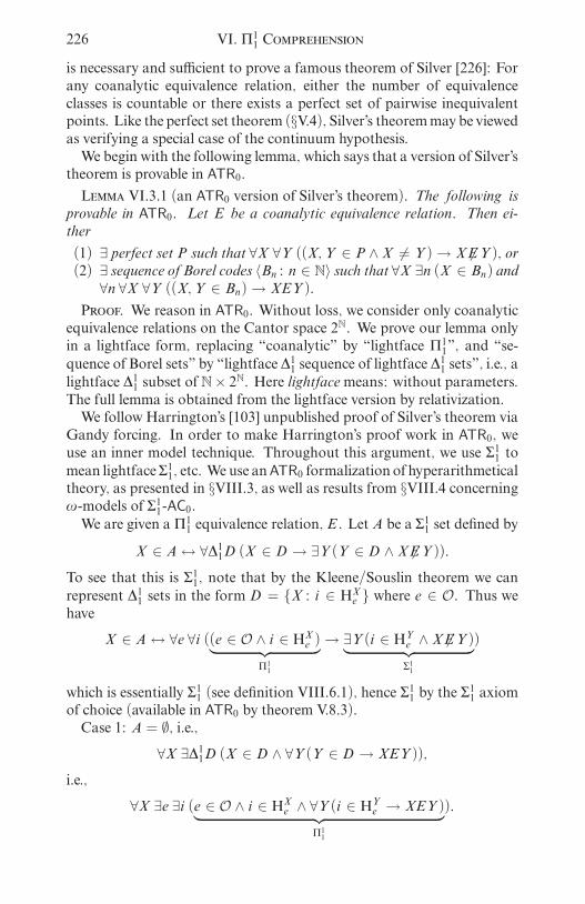
i

i

i

i

i

i

i

i


is necessary and sufficient to prove a famous theorem of Silver [226]: Forany coanalytic equivalence relation, either the number of equivalenceclasses is countable or there exists a perfect set of pairwise inequivalentpoints. Like the perfect set theorem (§V.4), Silver’s theoremmay be viewedas verifying a special case of the continuum hypothesis.We begin with the following lemma, which says that a version of Silver’stheorem is provable in ATR0.

Lemma VI.3.1 (an ATR0 version of Silver’s theorem). The following isprovable in ATR0. Let E be a coanalytic equivalence relation. Then ei-ther

(1) ∃ perfect set P such that ∀X ∀Y ((X,Y ∈ P ∧X 6= Y )→ X 6EY ), or(2) ∃ sequence of Borel codes 〈Bn : n ∈ N〉 such that ∀X ∃n (X ∈ Bn) and

∀n ∀X ∀Y ((X,Y ∈ Bn)→ XEY ).Proof. We reason in ATR0. Without loss, we consider only coanalyticequivalence relations on the Cantor space 2N. We prove our lemma onlyin a lightface form, replacing “coanalytic” by “lightface Π11”, and “se-quence of Borel sets” by “lightface ∆11 sequence of lightface ∆

11 sets”, i.e., a

lightface ∆11 subset of N× 2N. Here lightfacemeans: without parameters.The full lemma is obtained from the lightface version by relativization.We follow Harrington’s [103] unpublished proof of Silver’s theorem viaGandy forcing. In order to make Harrington’s proof work in ATR0, weuse an inner model technique. Throughout this argument, we use Σ11 tomean lightface Σ11, etc. We use anATR0 formalization of hyperarithmeticaltheory, as presented in §VIII.3, as well as results from §VIII.4 concerningù-models of Σ11-AC0.We are given a Π11 equivalence relation, E. Let A be a Σ

11 set defined by

X ∈ A↔ ∀∆11D (X ∈ D → ∃Y (Y ∈ D ∧ X 6EY )).To see that this is Σ11, note that by the Kleene/Souslin theorem we canrepresent ∆11 sets in the form D = X : i ∈ HXe where e ∈ O. Thus wehave

X ∈ A↔ ∀e ∀i ((e ∈ O ∧ i ∈ HXe )︸︷︷︸Π11

→ ∃Y (i ∈ HYe ∧ X 6EY )︸︷︷︸Σ11

)

which is essentially Σ11 (see definition VIII.6.1), hence Σ11 by the Σ

11 axiom

of choice (available in ATR0 by theorem V.8.3).Case 1: A = ∅, i.e.,

∀X ∃∆11D (X ∈ D ∧ ∀Y (Y ∈ D → XEY )),i.e.,

∀X ∃e ∃i (e ∈ O ∧ i ∈ HXe ∧ ∀Y (i ∈ HYe → XEY )︸︷︷︸Π11

).

i

i

i

i

i

i

i

i


Apply Π11 number uniformization and Σ11 separation to get a ∆

11 sequence

〈(en , in) : n ∈ N〉 such that ∀n (en ∈ O) and∀X ∃n (in ∈ HXen ∧ ∀Y (in ∈ HYen → XEY )).

Put Bn = X : in ∈ HXen. Thus in this case we have conclusion (2).Case 2: A 6= ∅. In this case we shall obtain conclusion (1).Define A in a slightly different but equivalent way:

X ∈ A↔ ∀∆11D (X ∈ D → ∃X0, X1(X0, X1 ∈ D ∧X0 6EX1))↔ ∀e ∀i ((e ∈ O ∧ i ∈ HXe )︸︷︷︸

Π11

→ ∃X0, X1(i ∈ HX0e ,HX1e ∧X0 6EX1)︸︷︷︸Σ11

)

∧ ∀e (e ∈ O︸︷︷︸Π11

→ ∃HXe︸︷︷︸Σ11

).

By Σ11 choice we can find a countable ù-model

M |= ACA0 ∧ ∃X (X ∈ A)︸︷︷︸essentially Σ11

,

where we are using the previous definition of A.Caution: It is probably not the case that M |= “E is an equivalencerelation”. But this will not matter.

Sublemma VI.3.2. For any Σ11 set B we have

M |= A ∩ B 6= ∅ → ∃X0, X1 (X0, X1 ∈ A ∩ B ∧ X0 6EX1).Proof. We reason inM . Suppose the conclusion fails, i.e.,

∀X0, X1 (X0, X1 ∈ A ∩ B → X0EX1),i.e.,

∀X0 (X0 ∈ A ∩ B︸︷︷︸Σ11

→ ∀X1 (X1 ∈ A ∩ B → X0EX1)︸︷︷︸Π11

).

By Σ11 separation, there exists a ∆11 interpolant D0 = X : i0 ∈ HXe0,

e0 ∈ O. Thus we have∀X0 (X0 ∈ A ∩ B → X0 ∈ D0)

and

∀X0 (X0 ∈ D0 → ∀X1 (X1 ∈ A ∩ B → X0EX1)),i.e.,

∀X1 (X1 ∈ A ∩ B︸︷︷︸Σ11

→ ∀X0 (X0 ∈ D0 → X0EX1)︸︷︷︸Π11

).

i

i

i

i

i

i

i

i


By Σ11 separation, there exists a ∆11 interpolant D1 = X : i1 ∈ HXe1,

e1 ∈ O. Thus we have∀X1 (X1 ∈ A ∩ B → X1 ∈ D1)

and

∀X1 (X1 ∈ D1 → ∀X0 (X0 ∈ D0 → X0EX1)).Put D = D0 ∩D1. We then have

∀X (X ∈ A ∩ B → X ∈ D)and

∀X0, X1 (X0, X1 ∈ D → X0EX1).Hence by definition of A we have A ∩ D = ∅. Hence A ∩ B = ∅. Thisproves the sublemma. 2

We now define Gandy forcing over M . A condition is a Σ11 set B suchthat M |= B 6= ∅. The set of all conditions is denoted C. Note thatA itself is a condition, i.e., A ∈ C, by case assumption and our choiceof M . Forcing and genericity over M are defined in the usual way. Aset D of conditions is said to be open if B ∈ D, B ′ ∈ C, B ′ ⊆ B implyB ′ ∈ D. D is said to be dense if it is open and for all conditions C thereexists a condition B ⊆ C such that B ∈ D. D is said to beM -definableif it is definable over M . X ∈ 2N is said to meet D if X ∈ B for someB ∈ D. X is said to be generic if it meets all dense, M -definable sets ofconditions. A condition B is said to force ϕ(X ), abbreviated B ‖− ϕ(X ),if ϕ(X ) holds for all generic X ∈ B. Note that for all conditions B wehaveB ‖− X ∈ B. We assume familiarity with basic properties of forcingand genericity.

Sublemma VI.3.3. If X0 ⊕ X1 is generic, then X0 and X1 are generic.Proof. By symmetry we consider only X0. Given a dense set D0, weneed to show that X0 meets D0. Consider

D = B ∈ C : X0 : ∃X1(X0 ⊕ X1 ∈ B) ∈ D0.We claim that D is dense. Given C ∈ C, put C0 = X0 : ∃X1(X0 ⊕X1 ∈ C ). Since D0 is dense, there exists B0 ∈ D0 such that B0 ⊆ C0. PutB = X0 ⊕X1 : X0 ⊕X1 ∈ C ∧X0 ∈ B0. Then B ∈ D and B ⊆ C . Thisproves the claim. Since X0 ⊕ X1 is generic, there exists B ∈ D such thatX0 ⊕ X1 ∈ B. Then X0 ∈ X0 : ∃X1 (X0 ⊕ X1 ∈ B) ∈ D0. This provesthe sublemma. 2

We consider product Gandy forcing C ×C overM . Conditions are nowCartesian products B ×C where B,C ∈ C. Choose an ù-modelN whichcontains (the code of)M and satisfies the Σ11 axiom of choice. Note thatHYP(M ) ⊆ N . We consider forcing and genericity overM with respect

i

i

i

i

i

i

i

i


to dense sets in N . We define B × C ‖− ϕ(X,Y ) to mean that ϕ(X,Y )holds for all generic (X,Y ) ∈ B×C . Note thatB×C ‖− X ∈ B,Y ∈ C .Sublemma VI.3.4. A×A ‖− X 6EY .Proof. Suppose for a contradiction that (X,Y ) ∈ A×A is generic andXEY , i.e., TE(X,Y ) is well founded. Thus we have |TE(X,Y )| ≤ α forsome α < ùX⊕Y1 ≤ ùM1 , which we denote by XEαY . (Note that Eαneed not be an equivalence relation.) By genericity, there exist conditionsB,C ⊆ A such that B × C ‖− XEαY . Put B ′ = X0 ⊕ X1 : X0, X1 ∈B,X0 6EX1. By sublemma VI.3.2 we have M |= (B ′ 6= ∅). Let (X0 ⊕X1, Y ) ∈ B ′ × C be generic. By a variant of sublemma VI.3.3, (X0, Y )and (X1, Y ) are generic. Since (X0, Y ), (X1, Y ) ∈ B×C , we haveX0EαY ,X1EαY , X0 6EX1, a contradiction. This proves the sublemma. 2

Now starting withAwe can build a full binary tree of conditions so thateach pair of paths is generic. Since each pair of paths belongs to A × A,sublemma VI.3.4 implies that we have a perfect set P such that

∀X ∀Y ((X ∈ P ∧ Y ∈ P ∧ X 6= Y )→ X 6EY ).

This completes the proof of lemma VI.3.1. 2

Definition VI.3.5 (Silver’s theorem). By Silver’s theorem we mean thefollowing statement: If E is a coanalytic equivalence relation, then eitherVI.3.1(1) holds, or

(2′) ∃ sequence of points 〈Yn : n ∈ N〉 such that ∀X ∃n (XEYn).

Theorem VI.3.6 (Silver’s theorem and Π11-CA0). The following arepair-wise equivalent over RCA0.

(i) Π11 comprehension.(ii) Silver’s theorem.(iii) Silver’s theorem restricted to equivalence relations onNN which are ∆02

definable (with parameters, of course).

Proof. Since Π11-CA0 includes ATR0, lemma VI.3.1 implies that Π11-CA0 proves (1) ∨ (2) for any coanalytic equivalence relation E. Butif (2) holds, then we can use Π11 comprehension to form n : Bn 6= ∅,followed by Σ11 choice to obtain a sequence of points 〈Yn : n ∈ N〉 suchthat ∀n (Bn 6= ∅ → Yn ∈ Bn), and this gives (2′). Thus we see thatΠ11-CA0

proves (1) ∨ (2′). We have shown (i)→(ii), and (ii)→(iii) is trivial.For the reversal, we reason in RCA0 and assume (iii). As in the proofof lemma VI.1.1, it is easy to show that (iii) implies arithmetical compre-hension. Given a Σ11 formula ϕ(m), use the Kleene normal form theorem(lemma V.1.4) to write ϕ(m) ≡ ∃f è(m,f), f ∈ NN, where è(m,f) isΠ01. Define a ∆

02 equivalence relation E on N × NN ∼= NN by putting

(m,f)E(n, g) ≡ m = n ∧ (è(m,f)↔ è(n, g)).

i

i

i

i

i

i

i

i


Clearly (1) does not hold for this equivalence relation, so by (2′) let〈Yk : k ∈ N〉 be a sequence of points of N × NN such that ∀m ∀f ∃k((m,f)EYk). Put Yk = (mk , fk). Then ∀m (∃f è(m,f) ↔ ∃k (m =mk ∧ è(m,fk)). Hence m : ϕ(m) = m : ∃f è(m,f) exists by arith-metical comprehension, using 〈(mk , fk) : k ∈ N〉 as a parameter. Thisproves Σ11 comprehension, hence (i). 2

Notes for §VI.3. Silver’s original proof of Silver’s theorem [226] usedtransfinitely many iterations of the power set axiom in ZFC. The factthat Silver’s theorem is provable in Z2 is due to Harrington [103]. Otherapplications of Harrington’s method are in Louveau [164]. The reversalin theorem VI.3.6 is due to Ramez Sami (personal communication, June1981). Lemma VI.3.1 and theorem VI.3.6 are due to Simpson (unpub-lished notes, March 17, 1984). For another treatment of lemma VI.3.1and related results, see Marcone [172]. Other results related to Silver’stheorem are in Harrington/Marker/Shelah [105], Louveau [165], andLouveau/Saint-Raymond [166].

VI.4. Countable Abelian Groups

In this section we show that Π11-CA0 is equivalent over RCA0 to a wellknown theorem concerning the structure of countable Abelian groups.Our result is as follows:

Theorem VI.4.1 (Π11-CA0 and countable Abelian groups). The follow-ing are equivalent over RCA0.

1. Π11 comprehension.2. Every countable Abelian group is a direct sum of a divisible group anda reduced group.

Proof. We shall need the following lemma.

Lemma VI.4.2. The following is provable in ACA0. If D is a divisiblesubgroup of a countable Abelian group G , then G = D ⊕ A for somesubgroupA.

Proof. By injectivity (theorem III.6.5) there is a homomorphism h :G → D such that h(d ) = d for all d ∈ D. Letting A be the kernel of h,i.e., A = a ∈ G : h(a) = 0, we easily see that G = D ⊕A. This provesthe lemma. 2

Now to prove theorem VI.4.1, assume Π11-CA0 and let G be an Abeliangroup. Let us define an element d ∈ G to be divisible if for each prime pthere exists f : N → G such that f(0) = d and ∀n (pf(n + 1) = f(n)).Being divisible is a Σ11 property, so by Σ

11 comprehension, D = d ∈ G :

d is divisible exists. Clearly D is a subgroup of G and is p-divisible forall primes p. By an easy application of Σ01 induction, it follows that D is

i

i

i

i

i

i

i

i

VI.4. Countable Abelian Groups 231

divisible. By lemma VI.4.2 we haveG = D ⊕A, and clearly A is reduced.This proves 1→ 2.For the converse, we reason in RCA0. We begin with:

Lemma VI.4.3. It is provable in RCA0 that statement 2 implies arithmeti-cal comprehension.

Proof. Reasoning in RCA0, let f : N → N be one-to-one. Let G be theAbelian group with generators xm, ym,i , m, i ∈ N and relations pxm = 0,pym,i+1 = ym,i , pym,0 = xf(m). The elements of G can be written innormal form as finite sums

∑km,iym,i +

∑lmxm, 0 < km,i < p. By our

assumption 2 we haveG = D ⊕R where D is divisible and R is reduced.We claim that, for each n ∈ N, xn ∈ D if and only if n ∈ rng(f). Tosee this, suppose xn ∈ D and let d =

∑km,iym,i +

∑lmxm be in D with

pd = xn. Note that

pd =∑

i>0

km,iym,i−1 +∑

i=0

km,ixf(m) = xn.

By uniqueness of the normal form, we have km,i = 0 for i > 0, km,0 = 0for m such that f(m) 6= n, and km,0 = 1 for m such that f(m) = n.Thus n ∈ rng(f). Conversely, suppose n = f(m) for some m. Then thesequence ym,0, ym,1, . . . p-divides xn. If xn /∈ D, then using G = D ⊕ Rwe have xn = d + r and ym,i = di + ri for each i . It follows that pri+1 = rifor all i , and pr0 = r 6= 0. Let A be the subgroup generated by r0, r1, . . . .It is easy to see that A exists, A is divisible, and A ⊆ R, a contradiction.The claim implies that rng(f) exists. By lemma III.1.3 this gives arith-metical comprehension, Q.E.D. 2

Nowwe use 2 plus arithmetical comprehension to proveΠ11 comprehen-sion. Given a tree T ⊆ N<N, let G be the Abelian group with generatorsxô , ô ∈ T , and relations pxô = xó , ô = óa〈i〉, and x〈〉 = 0. The ele-ments of G can be written in normal form as finite sums

∑kôxô where

0 < kô < p. By our assumption 2,G can be decomposed asD⊕R whereD is divisible and R is reduced. By lemma VI.4.2, D is the union of alldivisible subgroups of G .We claim that ô ∈ T lies on a path of T if and only if xô ∈ D. To seethis, note first that iff is a path throughT then the subgroupA generatedby xf[n], n ∈ N is divisible, hence A ⊆ D. Conversely, if xô ∈ D, useprimitive recursion to define a sequence dn ∈ D, n ∈ N, where d0 = xôand pdn+1 = dn for all n. If dn =

∑kóxó and dn+1 =

∑lñxñ, then

dn =∑kóxó = pdn+1 =

∑plñxñ, from which it follows that each ó

appearing in dn is a proper initial segment of some ñ appearing in dn+1.By primitive recursion there exists a sequence ón, n ∈ N, such that ó0 = ôand for all n, ón appears in dn and is a proper initial segment of ón+1.Thus ô lies on a path through T . This proves our claim.

i

i

i

i

i

i

i

i


Since D exists, our claim implies the existence of T = ô : ô lies on apath of T. This gives Π11 comprehension, in view of the following easylemma.

Lemma VI.4.4. Π11 comprehension is equivalent over RCA0 to the follow-ing statement S: For any tree T ⊆ N<N, there exists a subtree

T = ô : ô lies on a path of T.Proof. Obviously Π11-CA0 proves statement S. For the converse, as-sume statement S and let 〈Tk : k ∈ N〉 be an arbitrary sequence of trees.Form a tree

T = 〈〉 ∪ 〈k〉aô : k ∈ N, ô ∈ Tk.

By statement S, T exists. We have ∀k (〈k〉 ∈ T ↔ Tk has a path), henceby ∆01 comprehension k : Tk has a path exists. Now lemma VI.1.1 givesΠ11 comprehension. Lemma VI.4.4 is proved. 2

The proof of theorem VI.4.1 is now complete. 2

Remark VI.4.5. Combining theorem VI.4.1 with the results of §§III.6andV.7, we see thatΠ11-CA0 is necessary and sufficient for the developmentof the structure theory of countable Abelian groups, although ACA0 andATR0 suffice for certain parts of the theory. Such conclusions are typicalof Reverse Mathematics.

Notes for §VI.4. A nice exposition of the structure theory of countableAbelian groups is in Kaplansky [136]. The construction used in the lastpart of the proof of theorem VI.4.1 is from Feferman [58]. The theoremitself is due to Friedman/Simpson/Smith [78].

VI.5. Σ01 ∧Π01 Determinacy

We have seen in §V.8 that arithmetical transfinite recursion is equiva-lent to Σ01 determinacy. We shall now show that Π

11 comprehension is

equivalent to a stronger statement, namely Σ01 ∧Π01 determinacy.

Definition VI.5.1 (Σ01 ∧Π01 determinacy). A formula è is Σ01 ∧Π01 if itis of the form ϕ ∧ ø where ϕ is Σ01 and ø is Π01. Σ01 ∧ Π01 determinacy isthe scheme

∃S0 ∀S1 è(S0 ⊗ S1) ∨ ∃S1 ∀S0 ¬è(S0 ⊗ S1)where è(f) is Σ01 ∧ Π01. Here S0 and S1 are variables ranging over 0-strategies and 1-strategies respectively, as in §V.8.Lemma VI.5.2. Π11-CA0 proves Σ01 ∧Π01 determinacy.

i

i

i

i

i

i

i

i

VI.5. Σ01 ∧Π01 Determinacy 233

Proof. We reason in Π11-CA0. Let

ø(f) ≡ ϕ0(f) ∧ ¬ϕ1(f)be a Σ01 ∧Π01 formula, where ϕ0 and ϕ1 are Σ01. We shall prove

∃S′0 ∀S1 ø(S′0 ⊗ S1) ∨ ∃S′1 ∀S0 ¬ø(S0 ⊗ S′1).By theKleenenormal formtheoremV.1.4, wehaveϕi(f) ≡ ∃n èi(f[n]),where èi(ó) is arithmetical. Recall from §V.8 that

Seq0 = ó ∈ Seq: lh(ó) is even.We may safely assume that ϕi (f) ≡ ∃n èi(f[2n]) and that

(∀ó ∈ Seq0)∀n ((èi(ó) ∧ 2n < lh(ó))→ ¬èi(ó[2n])).For ó ∈ Seq = N<N and f ∈ NN, let óaf be the concatenation, i.e.,óaf ∈ NN where

(óaf)(n) =

ó(n) if n < lh(ó),

f(n − lh(ó)) if n ≥ lh(ó).

Put ϕói (f) ≡ ϕi(óaf) and èói (ô) ≡ èi(óaô). Note that ϕói (f) ≡∃n èói (f[2n]).Define

P = ó ∈ Seq0 : è0(ó) ∧ ∃S0 ∀S1 ¬ϕó1 (S0 ⊗ S1).We claim that P exists by Σ11 comprehension. To see this, it suffices toshow that ∀S1 ¬ϕó1 (S0⊗S1) is equivalent to an arithmetical formula. Letus say that ô ∈ Seq0 is compatible with S0 if ∀n (2n < lh(ô) → ô(2n) =S0(ô[2n])). Then ∀S1 ¬ϕó1 (S0 ⊗ S1) is equivalent to ∀S1 ∀n ¬èó1 ((S0 ⊗S1)[2n]), i.e.,

(∀ô ∈ Seq0) (ô compatible with S0 → ¬èó1 (ô)),which is arithmetical. This proves our claim, i.e., P exists.Now consider the Σ01 formula ϕ(f) ≡ ∃n (f[2n] ∈ P), with parameterP. By theorem V.8.7 we have Σ01 determinacy in Π

11-CA0, hence either

∃S0 ∀S1 ∃n ((S0 ⊗ S1)[2n] ∈ P) or ∃S1 ∀S0 ∀n ((S0 ⊗ S1)[2n] /∈ P).Case 1: ∃S0 ∀S1 ∃n ((S0 ⊗ S1)[2n] ∈ P). Fix such a 0-strategy S0.By Σ11 choice, there exists a sequence of 0-strategies 〈Só0 : ó ∈ P〉 suchthat (∀ó ∈ P)∀S1 ¬ϕó1 (Só0 ⊗ S1). Note that Σ11 choice applies in thissituation, because as we have seen above, the formula ∀S1 ¬ϕó1 (S0 ⊗ S1)is equivalent to an arithmetical formula. Now define a 0-strategy S′0 byputting S′0(ô) = S0(ô) for all ô ∈ Seq0 such that ∀n (2n ≤ lh(ô)→ ô[2n] /∈P), and S′0(ó

aô) = Só0 (ô) for all ó ∈ P and all ô ∈ Seq0.Let S1 be any 1-strategy. Then there exists a unique n such that (S′0 ⊗S1)[2n] ∈ P. In particular ϕ0(S′0 ⊗ S1) holds. Moreover, putting ó =(S′0 ⊗ S1)[2n] for this n, we have S′0 ⊗ S1 = óaf where ∀m (f[2m] is

i

i

i

i

i

i

i

i


compatible with Só0 ). It follows that ¬ϕó1 (f) holds, i.e., ¬ϕ1(S′0 ⊗ S1).Thus in this case we have ∀S1 ø(S′0 ⊗ S1).Case 2: ∃S1 ∀S0 ∀n ((S0 ⊗ S1)[2n] /∈ P). Fix such a 1-strategy S1.Define Q = ó ∈ Seq0 : è0(ó) ∧ ó /∈ P. By Σ01 determinacy we have thatfor all ó ∈ Q there exists a 1-strategy S1 such that ∀S0 ϕó1 (S0 ⊗ S1).We claim that a choice principle applies, i.e., there exists a sequence of

1-strategies 〈Só1 : ó ∈ Q〉 such that (∀ó ∈ Q)∀S0 ϕó1 (S0⊗ Só1 ). To see this,we use an inner model. LetM be a countable coded â-model containingall the parameters of the formula ϕ1(f) (theorem VII.2.10). ThenM |=ATR0 (theorem VII.2.7). Hence M |= Σ01 determinacy (theorem V.8.7).For each ó ∈ Q we have ¬∃S0 ∀S1 ¬ϕó1 (S0 ⊗ S1), and this can be writtenas aΠ11 formula, hence it holds inM , sinceM is a â-model. It now follows

by Σ01 determinacy inM that, for each ó ∈ Q,M |= ∃S1 ∀S0 ϕó1 (S0⊗ S1).Using the code ofM as a parameter, we obtain a sequence of 1-strategies

〈Só1 : ó ∈ Q〉 such that, for each ó ∈ Q, Só1 ∈M andM |= ∀S0 ϕó1 (S0 ⊗Só1 ). SinceM is a â-model, it follows that for each ó ∈ Q, ∀S0 ϕó1 (S0⊗Só1 )is true. This proves our claim.Now define a 1-strategy S′1 by putting S

′1(ô) = S1(ô) for all ô ∈ Seq1

such that ∀n(2n < lh(ô) → ¬è0(ô[2n])), and S′1(óaô) = Só1 (ô) for allô ∈ Seq1 and all ó ∈ Seq0 such that è0(ó) holds.Let S0 be any 0-strategy. We have ∀n (S0⊗S′1)[2n] /∈ P. If ∀n ¬è0(S0⊗S′1)[2n]) then we have ¬ϕ0(S0 ⊗ S′1). Otherwise there is a unique n suchthat (S0 ⊗ S′1)[2n] ∈ Q. Putting ó = (S0 ⊗ S′1)[2n] for this n, we haveS0 ⊗ S′1 = óaf where ∀m (f[2m] is compatible with Só1 ). It follows thatϕó1 (f) holds, i.e., ϕ1(S0⊗S′1). Thus in this case we have ∀S0 ¬ø(S0⊗S′1).This completes the proof of lemma VI.5.2. 2

We now turn to the reversal.

Lemma VI.5.3. It is provable in RCA0 that Σ01 ∧Π01 determinacy implies

Π11 comprehension.

Proof. Assume Σ01 ∧ Π01 determinacy. By lemma V.8.5 we have arith-metical comprehension. We shall prove Π11 comprehension. Our proofwill be analogous to the proof of lemma V.8.5. By lemma VI.1.1 it sufficesto show: given any sequence of trees 〈Tk : k ∈ N〉, there exists a set Xsuch that ∀k (k ∈ X ↔ Tk has a path). Without loss of generality, wemay assume ∀k (〈〉 ∈ Tk).Intuitively, consider the following game. Player 0 chooses an integerk = f(0). Then player 1 attempts to build a pathf(1), f(3), . . . throughTk . If player 1 succeeds, he wins the game. Otherwise, player 0 waitsuntil the first n such that 〈f(1), f(3), . . . , f(2n + 1)〉 /∈ Tk . Then player0 attempts to build a pathf(2n+2),f(2n+4), . . . through Tk . If player0 succeeds, he wins the game. Otherwise, player 1 wins the game.

i

i

i

i

i

i

i

i

VI.5. Σ01 ∧Π01 Determinacy 235

It is clear that player 0 cannot have a winning strategy. Hence, byΣ01∧Π01 determinacy, player 1 has a winning strategy; call it S1. Let gk(0),gk(1), . . . be the sequence f(1),f(3), . . . chosen by player 1 according toS1 when player 0 begins the game with f(0) = k. Then

∀k (Tk has a path→ gk is a path through Tk).Hence the desired set X exists by arithmetical comprehension with pa-rameters 〈Tk : k ∈ N〉 and 〈gk : k ∈ N〉. This proves Π11 comprehension.We now formalize the above intuitive argument.Formally, let è(f) be the following Σ01 ∧Π01 formula:

∃n (〈f(1), f(3), . . . , f(2n + 1)〉 /∈ Tf(0)) ∧∀m ∀n((〈f(1), f(3), . . . , f(2n − 1)〉 ∈ Tf(0) ∧

〈f(1), f(3), . . . , f(2n + 1)〉 /∈ Tf(0))→(〈f(2n + 2), f(2n + 4), . . . , f(2n + 2m)〉 ∈ Tf(0))).

We claim that ∀S0 ∃S1¬è(S0 ⊗ S1). To see this, let S0 be given and setk = S0(〈〉). IfTk has a path, let g be such a path and putS1(ó) = g(n) forall ó of length 2n + 1. Otherwise let S1 : Seq1 → N be arbitrary. Puttingf = S0 ⊗ S1 we have in the first case∀n (〈f(1), f(3), . . . , f(2n + 1)〉 = 〈g(0), g(1), . . . , g(n)〉 ∈ Tk = Tf(0)),and in the second case

∀n ∃m (〈f(2n + 2), f(2n + 4), . . . , f(2n + 2m)〉 /∈ Tk = Tf(0)).In either case ¬è(f). This proves our claim.Hence by Σ01∧Π01 determinacy there existsS1 such that∀S0 ¬è(S0⊗S1).For all k define gk : N → N recursively by

gk(n) = S1(〈k, gk(0), 0, gk(1), 0, . . . , gk(n − 1), 0〉).We claim that ∀k (ifTk has a path, then gk is a path throughTk). Supposenot. Let k, n, and h be such that gk [n] ∈ Tk and gk[n + 1] /∈ Tkand ∀m(h[m] ∈ Tk). Define S0(〈〉) = k, S0(ó) = 0 for ó of length2m + 2 < 2n + 2, and S0(ó) = h(m) for ó of length 2n + 2m + 2, for allm. Then clearly è(S0⊗S1) holds, a contradiction. This proves our claim.By arithmetical comprehension let X be such that ∀k (k ∈ X ↔ gk is apath through Tk). The previous claim implies that ∀k (k ∈ X ↔ Tk hasa path). This completes the proof of lemma VI.5.3. 2

Summarizing, we have

Theorem VI.5.4. The following are equivalent over RCA0.

1. Π11 comprehension.2. Σ01 ∧Π01 determinacy.Proof. This is immediate from lemmas VI.5.2 and VI.5.3. 2

i

i

i

i

i

i

i

i


Notes for §VI.5. Theorem VI.5.4 is from Tanaka [263]. Earlier Steel[256, page 24] had announced that Π11 comprehension is equivalent todeterminacy for Boolean combinations of Σ01 formulas, but the detailshave not appeared. Other related results are in Tanaka [264]. See also§§V.8 and VI.7.

VI.6. The ∆02 Ramsey Theorem

We have seen in §V.9 that arithmetical transfinite recursion is equivalentto the Σ01 Ramsey theorem. We shall now show that Π

11 comprehension

is equivalent to the ∆02 Ramsey theorem, and to the arithmetical or Σ0∞

Ramsey theorem. See theorem VI.6.4 below.We begin with the reversal.

Lemma VI.6.1. It is provable in RCA0 that∆02-RT impliesΠ11 comprehen-

sion.

Proof. Reasoning in RCA0, assume the ∆02 Ramsey theorem, ∆02-RT

(definition V.9.1). Trivially ∆02-RT implies RT(3), hence by lemma III.7.5we have arithmetical comprehension. We want to prove Π11 comprehen-sion. Let 〈Tm : m ∈ N〉 be a sequence of trees. By lemma VI.1.1 it sufficesto prove the existence of the set m : Tm has a path.Recall from §V.9 the notion of a tree T being majorized by a functionf ∈ [N]N or by a finite sequence ó ∈ [N]<N. Note also that, by boundedKonig’s lemma, f majorizes T if only if ∀n (f[n] majorizes T ). Thus “fmajorizes T” can be written as a Π01 formula. Moreover, T has a path ifand only if ∃f ∈ [N]N such that f majorizes T .For k ∈ N and f ∈ [N]N, define f(k) ∈ [N]N by f(k)(n) = f(k + n).Write

ϕ(f) ≡ (∀m < f(0)) (f(1) majorizes Tm ↔ f(2) majorizes Tm).

Note that ϕ(f) can be written in either Σ02 or Π02 form, i.e., ϕ(f) is ∆

02.

By ∆02-RT, let h ∈ [N]N be homogeneous for ϕ(f), i.e., either (∀g ∈[N]N)ϕ(h · g) or (∀g ∈ [N]N)¬ϕ(h · g).Claim 1: ϕ(h · g) holds for all g ∈ [N]N.If not, then¬ϕ(h ·g) holds for all g ∈ [N]N, hence in particular for eachn ∈ N there exists m < h(0) such that Tm is majorized by h(n+2) but notby h(n+1). Mapping n to the least such m, we would obtain a one-to-onefunction from N into 0, 1, . . . , h(0)− 1, contradiction.Claim 2: For each m ∈ N, if Tm has a path then Tm is majorized byh(m+2).Suppose not, i.e., Tm has a path but h(m+2) does not majorize Tm. Letn ∈ N be such that h(m+2)[n] does not majorize Tm. Let g ∈ [N]N be such

i

i

i

i

i

i

i

i

VI.6. The ∆02 Ramsey Theorem 237

that g majorizes Tm . Put

f = h(m+1)[n + 1]a(h(m+n+2) · g).Then Tm is majorized by f

(n+1) = (h(m+n+2) · g) but is not majorized byf(1) = h(m+2)[n]a(h(m+n+2) ·g). This is a contradiction, since we havem <h(m + 1) = f(0) and therefore, by claim 1, for all k ≥ 1, f(k) majorizesTm if and only if f

(k+1) majorizes Tm. Thus we have proved claim 2.By claim 2 we have

∀m (Tm has a path↔ Tm is majorized by h(m+2)).Hence m : Tm has a path exists, by arithmetical comprehension with has a parameter. This completes the proof of lemma VI.6.1. 2

We shall now show that, for all k ∈ ù, Σ0k-RT is provable in Π11-CA0. Weuse an inner model technique. Our proof is based on the following lemma,which employs the notion of countable coded â-model from §VII.2. IfM1 andM2 are countable coded â-models,M1 ∈M2 means that the codeofM1 is an element ofM2.

Lemma VI.6.2. The following is provable in ACA0. LetM1, . . . ,Mk bea finite sequence of countable coded â-models such that

M1 ∈ · · · ∈Mk .Then for any Σ0k formula ϕ(f) with parameters inM1, there exists h ∈Mksuch that ∀g ϕ(h · g) ∨ ∀g ¬ϕ(h · g). Here f, g, and h range over [N]N.Proof. We reason in ACA0 and proceed by induction on k ≥ 1. ForΣ01 formulas, our result follows from Σ

01-RT in ATR0 (theorem V.9.7)

plus the fact that any countable coded â-model satisfies ATR0 (theoremVII.2.7). We inductively assume our result for Σ0k formulas and prove andprove it for Σ0k+1 formulas, k ≥ 1.Let M1 ∈ · · · ∈ Mk ∈ Mk+1 be countable coded â-models. Let ϕ(f)be a Σ0k+1 formula with parameters inM1. Write

ϕ(f) ≡ ∃n1 ∀n2 · · · nk ø(n1, n2, . . . , nk , f)where ø(n1, . . . , nk , f) is Σ

01 or Π

01, depending on whether k is even or

odd, with parameters inM1.WithinM2, by recursion on n ∈ N using the code ofM1 as a parameter,define sequences ón ∈ [N]<N, fn ∈ M1 ∩ [N]N, n ∈ N, as follows. Weemploy the concatenation notation óaf as in §VI.5. For each n ∈ Nwe shall have ónafn ∈ [N]N. Begin with ó0 = 〈〉 and f0 = the identityfunction, i.e., f0(m) = m for all m ∈ N. Given ónafn ∈ [N]N, putón+1 = óna〈fn(0)〉 and recall that f(1)n (m) = fn(m + 1) for all m ∈ N;thus ón+1af

(1)n = ónafn ∈ [N]N. By finitely many applications of Σ01-RT

in M1, obtain gn ∈ M1 ∩ [N]N such that, for all subsequences ó of ón+1

i

i

i

i

i

i

i

i


and all n1, . . . , nk ≤ n,

(∀h ∈ [N]N)ø(n1, . . . , nk , óa(f(1)n · gn · h))∨ (∀h ∈ [N]N)¬ø(n1, . . . , nk , óa(f(1)n · gn · h)).

Put fn+1 = f(1)n · gn. As part of the same recursion, define p : N × Nk ×

[N]<N → 0, 1 such that, for all n and all subsequences ó of ón+1 andn1, . . . , nk ≤ n,

p(n, n1, . . . , nk , ó) =

1 if (∀h ∈ [N]N)ø(n1, . . . , nk , óa(f(1)n · gn · h)),0 if (∀h ∈ [N]N)¬ø(n1, . . . , nk , óa(f(1)n · gn · h)).

Finally define f ∈ [N]N by f(n) = fn(0) for all n ∈ N; thus f[n] = ónfor all n ∈ N. Note that f ∈M2 and p ∈M2.By construction we have

ø(n1, . . . , nk , f · g)↔ ∃n (p(n, n1, . . . , nk , (f · g)[n]) = 1)and

¬ø(n1, . . . , nk , f · g)↔ ∃n (p(n, n1, . . . , nk , (f · g)[n]) = 0),for all n1, . . . , nk ∈ N and g ∈ [N]N. Thus

ø(n1, . . . , nk , g) ≡ ø(n1, . . . , nk , f · g)is ∆01 with parameters inM2. Hence

ϕ(g) ≡ ϕ(f · g)≡ ∃n1 ∀n2 · · ·nk ø(n1, . . . , nk , f · g)≡ ∃n1 ∀n2 · · ·nk ø(n1, . . . , nk , g)

is Σ0k with parameters inM2. Hence, by inductive hypothesis, there exists

h ∈Mk+1 ∩ [N]N such that ∀g ϕ(h ·g)∨∀g ¬ϕ(h ·g), i.e., ∀g ϕ(f ·h ·g)∨∀g ¬ϕ(f · h · g), where g ranges over [N]N. This completes the proof. 2

Lemma VI.6.3. Π11-CA0 proves Σ0∞-RT. In other words, for each k ∈ ù,Π11-CA0 proves Σ0k-RT.

Proof. Letϕ(f) be aΣ0k formula, k ≥ 1. Reasoning inΠ11-CA0, letX ⊆N be such that all the parameters of ϕ(f) are≤T X . By k applications oftheorem VII.2.10, we obtain countable coded â-models X ∈ M1 ∈ · · · ∈Mk . Then lemma VI.6.2 gives ∃h (∀g ϕ(h · g)∨∀g ¬ϕ(h · g)), i.e., Σ0k-RTfor ϕ(f). This proves the lemma. 2

The main result of this section is:

Theorem VI.6.4. The following are pairwise equivalent over RCA0:

1. Π11 comprehension;2. the ∆02 Ramsey theorem;3. the Σ0∞ Ramsey theorem.

i

i

i

i

i

i

i

i

VI.7. Stronger Set Existence Axioms 239

Proof. This is immediate from lemmas VI.6.3 and VI.6.1. 2

Notes for §VI.6. Lemma VI.6.1 is due to Simpson (unpublished notes,June 1981). Lemma VI.6.3 is related to results of Solovay [252]. See alsoTanaka [262]. Related results are in §§III.7, V.9, VI.7.

VI.7. Stronger Set Existence Axioms

We have seen (in §§V.8 and V.9) that ATR0 is just strong enough toprove Σ01 determinacy and the Σ

01 Ramsey theorem. We have also seen

(in §§VI.5 and VI.6) that Π11-CA0 is just strong enough to prove Σ01 ∧Π11determinacy and the Σ0∞ Ramsey theorem. The purpose of this sectionis to point out that stronger forms of determinacy and Ramsey’s theoremrequire stronger set existence axioms.In analogy with arithmetical transfinite recursion (ATR0, §V.2), thescheme of Π11 transfinite recursion is defined as follows.

Definition VI.7.1 (Π11 transfinite recursion). We define Π11-TR0 to be

the formal system consisting of ACA0 plus Π11 transfinite recursion, i.e.,

∀X (WO(X )→ ∃Y Hè(X,Y ))where è is any Π11 formula.For 2 ≤ k < ∞, the system Π1k-TR0 is defined similarly, with Π11replaced by Π1k .

Remark VI.7.2. Some results onmodels ofΠ11-TR0 and related systemsare in chapters VII and VIII.


1. Π11 transfinite recursion;2. ∆02 determinacy;3. the ∆11 Ramsey theorem.

Proof. We omit the proofs, which can be found in Tanaka [262, 263].2

Remark VI.7.4. The previous theorem is due to Tanaka. In addi-tion, Tanaka defined a stronger subsystem of Z2, Σ11-MI0 (related to Σ11monotonic recursion and Σ11 reflecting ordinals), and proved the follow-ing theorem.


1. Σ11-MI0;2. Σ02 determinacy;3. the Σ11 Ramsey theorem.

Proof. See Tanaka [262, 264]. 2

i

i

i

i

i

i

i

i


Remark VI.7.6 (stronger formsof Ramsey’s theorem). TheBorelRam-sey theorem, i.e., the ∆11 Ramsey theorem, is also known as the Galvin/Prikry theorem; see Mathias [181] and Carlson/Simpson [33]. We haveseen above that the Galvin/Prikry theorem and indeed the Σ11 Ramseytheorem are provable in Z2. On the other hand, it is known that the ∆12Ramsey theorem is not provable in ZFC. This follows from the fact thatthe canonical well ordering of P(ù) in L(X ) is Σ12 (definition VII.4.20,lemma VII.4.21, sublemma VII.6.8).

Remark VI.7.7 (stronger forms of determinacy). Friedman [66] hasshown that Σ05 determinacy is not provable in Z2. Martin [177, 178]has shown that Borel determinacy is provable in ZFC. Friedman [66, 71]has shown that the proof of Borel determinacy requires ℵ1 applicationsof the power set axiom. Friedman [65] has shown that Σ11 determinacy isnot provable in ZFC; indeed, it is false in all forcing extensions of L(X ).Harrington [104] has improved this by showing that Σ11 determinacy isequivalent to ∀X (X # exists).

Notes for §VI.7. Theorems VI.7.3 and VI.7.5 are due to Tanaka [262, 263,264]. A result along the lines of 1↔ 2 of VI.7.3 was announced by Steel[256, page 24], but the proof has not been published. Regarding 1 ↔ 2of VI.7.5, see also Steel [256, pages 24–25] and Moschovakis [191, pages414–415]. Regarding 1 ↔ 3 of VI.7.5, see also Solovay [252]. For moreon Σ11 monotonic recursion and Σ

11 reflecting ordinals, see Richter/Aczel

[206], Aanderaa [1], and Simpson [233].

VI.8. Conclusions

In this chapterwe have seen that severalmathematical theorems are logi-cally equivalent to Π11-CA0. Among them are: the Cantor/Bendixson the-orem for closed sets (§VI.1), Kondo’s theorem on coanalytic uniformiza-tion (§VI.2), Silver’s theoremonBorel equivalence relations (§VI.3), a keystructure theorem for countable Abelian groups (§VI.4), the ∆02 Ramseytheorem (§VI.6), and Σ01 ∧ Π01 determinacy (§VI.5). We have also seen(§VI.7) that stronger forms of Ramsey’s theorem and determinacy requirestronger set existence axioms.Our proof techniques in this chapter have been based mostly on theKleene normal form theorem, via lemmaVI.1.1 concerning paths throughtrees. We have also used an inner model technique (see lemmas VI.5.2and VI.6.2) involving countable coded â-models (§VII.2).

i

i

i

i

i

i

i

i

Part B

MODELS OF SUBSYSTEMS OF Z2

i

i

i

i

i

i

i

i

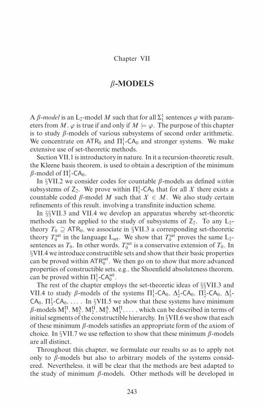
i

i

i

i

i

i

i

i

Chapter VII

â-MODELS

A â-model is an L2-modelM such that for all Σ11 sentences ϕ with param-eters fromM , ϕ is true if and only ifM |= ϕ. The purpose of this chapteris to study â-models of various subsystems of second order arithmetic.We concentrate on ATR0 and Π11-CA0 and stronger systems. We makeextensive use of set-theoretic methods.Section VII.1 is introductory in nature. In it a recursion-theoretic result,the Kleene basis theorem, is used to obtain a description of the minimumâ-model of Π11-CA0.In §VII.2 we consider codes for countable â-models as defined withinsubsystems of Z2. We prove within Π11-CA0 that for all X there exists acountable coded â-model M such that X ∈ M . We also study certainrefinements of this result, involving a transfinite induction scheme.In §§VII.3 and VII.4 we develop an apparatus whereby set-theoreticmethods can be applied to the study of subsystems of Z2. To any L2-theory T0 ⊇ ATR0, we associate in §VII.3 a corresponding set-theoretictheory T set0 in the language Lset. We show that T

set0 proves the same L2-

sentences as T0. In other words, T set0 is a conservative extension of T0. In§VII.4 we introduce constructible sets and show that their basic propertiescan be proved within ATR

set0 . We then go on to show that more advanced

properties of constructible sets, e.g., the Shoenfield absoluteness theorem,can be proved within Π11-CA

set0 .

The rest of the chapter employs the set-theoretic ideas of §§VII.3 andVII.4 to study â-models of the systems Π11-CA0, ∆12-CA0, Π12-CA0, ∆13-CA0, Π13-CA0, . . . . In §VII.5 we show that these systems have minimumâ-modelsMΠ1 , M

∆2 , M

Π2 , M

∆3 , M

Π3 , . . . , which can be described in terms of

initial segments of the constructible hierarchy. In §VII.6 we show that eachof these minimum â-models satisfies an appropriate form of the axiom ofchoice. In §VII.7 we use reflection to show that these minimum â-modelsare all distinct.Throughout this chapter, we formulate our results so as to apply notonly to â-models but also to arbitrary models of the systems consid-ered. Nevertheless, it will be clear that the methods are best adapted tothe study of minimum â-models. Other methods will be developed in

243

i

i

i

i

i

i

i

i

244 VII. â-Models

chapters VIII and IX, in order to constructù-models and non-ù-models,respectively.

VII.1. The Minimum â-Model ofΠ11-CA0

Definition VII.1.1 (ù-models). An ù-model is an L2-model M suchthat the first order part of M is the standard model (ù,+, ·, 0, 1, <) ofZ1. We sometimes identifyM with the set SM ⊆ P(ù). Here P(ù) is thepowerset of ù.

Definition VII.1.2 (â-models). A â-model is anù-modelM such thatfor any Σ11 sentence ϕ with parameters fromM ,M |= ϕ if and only if ϕis true.

The purpose of this chapter is to study â-models of various subsystemsof Z2. In the present introductory section, we study â-models of Π11-CA0.Weprove that there exists aminimum (i.e., unique smallest)â-model ofΠ11-CA0 (corollary VII.1.10). At the same time we obtain a characterizationof â-models of Π11-CA0 bymeans of the hyperjump (theoremVII.1.8). Wealso present a more general result which characterizes â-submodels of anarbitrary given model of Π11-CA0 (definition VII.1.11, theorem VII.1.12).Some of the ideas which are introduced here will be refined and gen-eralized in later sections of this chapter. For instance, in §VII.5 we shallobtain an alternative description of the minimum â-model of Π11-CA0, bymeans of constructible sets.Our first goal is to prove a formal version of a well known recursion-theoretic result known as the Kleene basis theorem. We begin with defini-tions of relative recursiveness and the hyperjump. For general backgroundon recursion theory theory and hyperarithmetical theory, see for instanceKleene [142], Rogers [208], Shoenfield [222, chapters 6 and 7], and Sacks[211, part A].

Definition VII.1.3 (universal lightface Π01 formula). Let

ð(e,m1, . . . , mi , X1, . . . , Xj)

be aΠ01 formulawith exactly the displayed free variables. (Herem1, . . . , miare free number variables, X1, . . . , Xj are free set variables, and e is adistinguished free number variable.) We say that ð is universal lightfaceΠ01 if for all Π

01 formulas ð

′ with the same free variables as ð, RCA0 proves

∀e ∃e′ ∀m1 · · · ∀X1 · · · (ð(e′, m1, . . . , X1, . . . )↔ ð′(e,m1, . . . , X1, . . . )).It is known that for all numbers of variables i, j < ù there exists a universallightface Π01 formula. The existence of such formulas is closely related tothe enumeration theorem in recursion theory.

i

i

i

i

i

i

i

i

VII.1. The Minimum â-Model of Π11-CA0 245

Definition VII.1.4 (relative recursiveness). The following definition ismade in RCA0. Let ð(e,m1, X1) be a fixed universal lightface Π01 formulawith exactly the displayed free variables. Given X,Y ⊆ N we say thatY is recursive in X or X -recursive (equivalently Y is Turing reducibleto X , written Y ≤T X ), if there exist e0, e1 ∈ N such that for all m,m ∈ Y ↔ ð(e1, m,X ) andm /∈ Y ↔ ð(e0, m,X ). In this case we say thate = (e0, e1) is an X -recursive index of Y .We say that X is Turing equivalent to Y , written X =T Y , if X ≤T Yand Y ≤T X . This is an equivalence relation on subsets of N. A Turingdegree is an =T-equivalence class.

Definition VII.1.5 (hyperjump). The following definition is made inRCA0. Let f be a function variable, i.e., f ranges over total functionsf : N → N. As usual we identify such a function with a set of orderedpairs f ⊆ N × N ⊆ N. Given X ⊆ N, the hyperjump of X , denotedHJ(X ), is the set of all (m, e) ∈ N × N ⊆ N such that ∃f ð(e,m,f,X ),if this set exists. Here ð(e,m1, X1, X2) is a fixed universal lightface Π01formula with exactly the displayed free variables.

The next lemma is a formal version of the fact thatHJ(X ) is “complete”among sets which are lightface Σ11 definable from X .

Lemma VII.1.6. Let ϕ(e,m,X ) be a Σ11 formula with only the displayedfree variables. The following is provable in ACA0. For all e ∈ N andX ⊆ N,if HJ(X ) exists then m : ϕ(e,m,X ) exists and is recursive in HJ(X ).Proof. By the proof of lemma V.1.4 (our formal version of the Kleenenormal form theorem), we obtain a Π01 formula

ð′(e,m,f,X )

with only the displayed free variables such that ACA0 proves

∀e ∀m ∀X (ϕ(e,m,X )↔ ∃f ð′(e,m,f,X )).Now reasoning within ACA0, given e let e′ be such that

∀m ∀f ∀X (ð(e′, m,f,X )↔ ð′(e,m,f,X ))where ð is our fixed universal lightfaceΠ01 formula as in definition VII.1.5.Given X such that HJ(X ) exists, let Y be the set of all m such that(m, e′) ∈ HJ(X ). Clearly Y ≤T HJ(X ) and ∀m (m ∈ Y ↔ ϕ(e,m,X )).This completes the proof. 2

The following lemma is our formal version of theKleene basis theorem.

Lemma VII.1.7 (formalized Kleene basis theorem). Let ϕ(m,Y,X ) bea Σ11 formula with only the displayed free variables. The following is provablein ACA0. Let X ⊆ N be given such that HJ(X ) exists. For all m, if∃Y ϕ(m,Y,X ) then ∃Y (Y ≤T HJ(X ) ∧ ϕ(m,Y,X )).

i

i

i

i

i

i

i

i

246 VII. â-Models

Proof. By the proof of lemma V.1.4, we obtain an arithmetical formulaè(m, ó, ô, X ) with only the displayed free variables, such thatACA0 proves

∀m ∀X ∀Y (ϕ(m,Y,X )↔ ∃f ∀n è(m,Y [n], f[n], X )).Now reasoning within ACA0, let X be given such that HJ(X ) exists. LetG be the set of all (m, ó, ô) ∈ N × 2<N × N<N such that

∃Y ∃f (∀n è(m,Y [n], f[n], X ) ∧ Y [lh(ó)] = ó ∧ f[lh(ô)] = ô).By lemma VII.1.6,G exists and is recursive in HJ(X ). Now letm be givensuch that ∃Y ϕ(m,Y,X ). Then clearly (m, 〈〉, 〈〉) ∈ G . Define Y (n) andf(n) by recursion on n as follows: Y (n) = 1 if (m,Y [n]a〈1〉, f[n]) ∈ G ;Y (n) = 0otherwise;f(n) = least j such that (m,Y [n+1], f[n]a〈j〉) ∈ G .ClearlyY andf are recursive inG and, by ∆01 induction, (m,Y [n], f[n]) ∈G for all n ∈ N. In particular ∀n è(m,Y [n], f[n], X ) so ϕ(m,Y,X ) holds.Also Y ≤T HJ(X ) by transitivity of≤T, sinceY ≤T G andG ≤T HJ(X ).This completes the proof. 2

It can also be shown that lemmas VII.1.6 and VII.1.7 are provable inRCA0 (rather than ACA0).We are now ready to present the following characterization of â-modelsof Π11-CA0.

Theorem VII.1.8 (â-models of Π11-CA0). LetM beanù-model ofRCA0.The following are equivalent.

1. M is a â-model ofΠ11-CA0.2. M is closed under hyperjump, i.e., HJ(X ) ∈M for all X ∈M .Proof. Suppose first thatM is a â-model of Π11-CA0. Let ð be Π01 asin the definition of hyperjump (definition VII.1.5). Given X ∈ M , byΣ11 comprehension within M let Y ∈ M be the set of all (m, e) suchthat M |= ∃f ð(e,m,f,X ). Since M is a â-model, we have M |=∃f ð(e,m,f,X ) if and only if ∃f ð(e,m,f,X ) is true, for all e and m.Hence Y = HJ(X ). Hence HJ(X ) ∈M . This proves that 1 implies 2.For the converse, letM be an ù-model of RCA0 which is closed underhyperjump. We must show that M is a â-model of Π11-CA0. Let ϕ(m)be Σ11 with no free variables other than m, but with parameters fromM .Let X ∈ M be such that all of the parameters of ϕ(m) are recursivein X . Thus ϕ(m) can be written as ∃Y è(m,Y,X ) where è(m,Y,X ) isarithmetical with no free variables other thanm andY , and no parametersother than X . By assumption HJ(X ) ∈ M . Hence Y ∈ M for allY ≤T HJ(X ). Hence by the Kleene basis theorem VII.1.7, we see that foreachm,M |= ∃Y è(m,Y,X ) if and only if ∃Y è(m,Y,X ) is true. In otherwords, M |= ϕ(m) if and only if ϕ(m) is true. This shows that M is aâ-model. Furthermore, by lemma VII.1.6, the setZ = m : ϕ(m) is trueis recursive in HJ(X ). Hence Z ∈ M andM |= ∀m (m ∈ Z ↔ ϕ(m)).Thus M |= Σ11 comprehension, or equivalently Π11 comprehension. Theproof is complete. 2

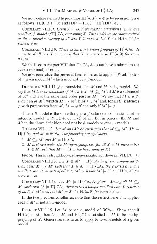
i

i

i

i

i

i

i

i

VII.1. The Minimum â-Model of Π11-CA0 247

We now define iterated hyperjumps HJ(n,X ), n ∈ ù by recursion on nas follows: HJ(0, X ) = X and HJ(n + 1, X ) = HJ(HJ(n,X )).

Corollary VII.1.9. Given X ⊆ ù, there exists a minimum (i.e., uniquesmallest)â-model ofΠ11-CA0 containingX . Thismodel can be characterizedas the ù-model consisting of all sets Y ⊆ ù such that Y ≤T HJ(n,X ) forsome n ∈ ù.Corollary VII.1.10. There exists a minimum â-model of Π11-CA0. Itconsists of all sets X ⊆ ù such that X is recursive in HJ(n, ∅) for somen ∈ ù.We shall see in chapter VIII that Π11-CA0 does not have a minimum (oreven a minimal) ù-model.We now generalize the previous theorem so as to apply to â-submodelsof a given modelM ′ which need not be a â-model.

Definition VII.1.11 (â-submodels). LetM andM ′ be L2-models. Wesay thatM is anù-submodel of M ′, writtenM ⊆ù M ′, ifM is a submodelof M ′ and has the same first order part as M ′. We say that M is a â-submodel of M ′, writtenM ⊆â M ′, ifM ⊆ù M ′ and, for all Σ11 sentencesϕ with parameters fromM ,M |= ϕ if and only ifM ′ |= ϕ.Thus a â-model is the same thing as a â-submodel of the standard orintended model (ù,P(ù),+, ·, 0, 1, <) of Z2. But in general, theM andM ′ in the above definition need not be â-models or even ù-models.

Theorem VII.1.12. LetM andM ′ be given such thatM ⊆ù M ′,M ′ |=Π11-CA0, andM |= RCA0. The following are equivalent.

1. M ⊆â M ′ andM |= Π11-CA0.2. M is closed under theM ′-hyperjump, i.e., for all X ∈M there existsY ∈M such thatM ′ |= (Y is the hyperjump of X ).

Proof. This is a straightforward generalization of theoremVII.1.8. 2

Corollary VII.1.13. Let X ∈ M ′ |= Π11-CA0 be given. Among all â-submodelsM ⊆â M ′ such that X ∈ M |= Π11-CA0, there exists a uniquesmallest one. It consists of all Y ∈M ′ such thatM ′ |= Y ≤T HJ(n,X ) forsome n ∈ ù.Corollary VII.1.14. Let M ′ |= Π11-CA0 be given. Among all M ⊆âM ′ such thatM |= Π11-CA0, there exists a unique smallest one. It consistsof all X ∈M ′ such thatM ′ |= X ≤T HJ(n, ∅) for some n ∈ ù.In the two previous corollaries, note that the restriction n ∈ ù applieseven ifM ′ is not an ù-model.

Exercise VII.1.15. Let M be an ù-model of RCA0. Show that ifHJ(X ) ∈ M , then X ∈ M and HJ(X ) is satisfied in M to be the hy-perjump of X . Generalize this so as to apply to ù-submodels of a givenmodel.

i

i

i

i

i

i

i

i

248 VII. â-Models

Exercise VII.1.16. Show that Π11-CA0 is equivalent over RCA0 to theassertion that for all X , HJ(X ) exists.

Exercise VII.1.17. Recall from §VI.7 that Π11-TR0 consists of RCA0

plus all axioms ∀Y (WO(Y ) → ∃ZHè(Y,Z)) where è(n,Z) is any Π11formula. Show that Π11-TR0 is equivalent over RCA0 to the assertion that∀X ∀Y (WO(Y ) → the hyperjump can be iterated along Y starting withX ).

Exercise VII.1.18. Give a characterization of â-models of Π11-TR0analogous to theorem VII.1.8. Prove that there exists a minimum â-model of Π11-TR0. Prove that for any model of Π11-TR0 there is a smallestâ-submodel of Π11-TR0.

It is natural to ask whether there exists a minimum â-model of ATR0.This question is answered negatively by the following result, which will beproved in chapter VIII; see corollary VIII.6.9.

Theorem VII.1.19. LetM ′ be any countablemodel ofATR0. Then thereexists a proper â-submodelM ⊆â M ′,M 6=M ′. For any suchM we havealsoM |= ATR0.

Corollary VII.1.20. There is no minimum â-model of ATR0.

Exercise VII.1.21. Show that any â-model is a model of ATR0. Moregenerally, show that ifM ⊆â M ′ andM ′ |= ATR0, thenM |= ATR0.

Further results on â-models of ATR0 will be presented in §VII.2 andin chapter VIII. Further results on â-models of Π11-CA0 and strongertheories will be presented in §§VII.5, VII.6 and VII.7.Notes for §VII.1. The Kleene basis theorem is due to Kleene [143]. Ourcharacterization of â-models of Π11-CA0 in terms of ≤T and HJ (theoremVII.1.8) is well known. A set-theoretic characterization of such models isgiven in exercise VII.3.36. The minimum â-model of Π11-CA0 can also bedescribed in terms of constructible sets; see theorem VII.5.17.

VII.2. Countable Coded â-Models

In this section we consider countable â-models which are encoded assingle subsets of N. We show that Π11-CA0 is strong enough to prove theexistence of such models. We also study a formal theory of transfiniteinduction which is satisfied by all such models.We begin by giving a definition within RCA0 of codes for countableù-models together with the appropriate satisfaction concept. Recall thatany set X ⊆ N can be viewed as a code for a countable sequence of sets〈(X )n : n ∈ N〉 where (X )n = i : (i, n) ∈ X.

i

i

i

i

i

i

i

i

VII.2. Countable Coded â-Models 249

Definition VII.2.1 (countable coded ù-models). The followingdefini-tion is made within RCA0. A countable coded ù-model is a set W ⊆ N,viewed as encoding the L2-model

M = (N,SM ,+, ·, 0, 1, <)with

SM = (W )n : n ∈ N.Let SntM be the set of (Godel numbers of) sentences ofL2 with parametersfrom |M | ∪ SM , i.e., from N ∪ (W )n : n ∈ N. Given ϕ ∈ SntM , letSubM (ϕ) be the set of ø ∈ SntM such that ø is a substitution instance ofa subformula of ϕ. A valuation for ϕ is a function f : SubM (ϕ)→ 0, 1which obeys the following clauses:

f(t1 = t2) =

1 if t1 = t2,

0 if t1 6= t2;

f(t1 < t2) =

1 if t1 < t2,

0 if t1 ≥ t2;f(¬ø) = 1− f(ø);

f(ø1 ∧ ø2) =1 if f(ø1) = f(ø2) = 1,

0 otherwise;

f(∀mø(m)) =1 if f(ø(m)) = 1 for all m ∈ N,0 otherwise;

f(∀X ø(X )) =1 if f(ø((W )n)) = 1 for all n ∈ N,0 otherwise.

Clearly for any ϕ ∈ SntM there is at most one such valuation. We say thatM satisfies ϕ, writtenM |= ϕ, if there exists a valuationf for ϕ such thatf(ϕ) = 1. (This concept of satisfaction is similar to the notion of weakmodel which was introduced in §II.8.)

Lemma VII.2.2. Let ϕ be any sentence of L2. Then ACA0 proves the fol-lowing. For all countable codedù-modelsM there exists a unique valuationf : SubM (ϕ)→ 0, 1.Proof. The proof is straightforward by arithmetical comprehensionusing the code ofM as a parameter. 2

Fix a universal lightface Π01 formula ð(e,m1, m2, X1, X2, X3) with ex-actly the displayed free variables (definition VII.1.3). Let ϕ1(e,m,X,Y )be the Σ11 formula

∃Z ∀n ¬ð(e,m, n,X,Y,Z).

i

i

i

i

i

i

i

i

250 VII. â-Models

Thus ϕ1(e,m,X,Y ) is in some sense a universal lightface Σ11 formula withfree variables e,m,X,Y .

Definition VII.2.3 (countable coded â-models). A countable coded â-model is defined in RCA0 to be a countable coded ù-modelM such thatfor all e,m ∈ N and X,Y ∈ SM , ϕ1(e,m,X,Y ) if and only if M |=ϕ1(e,m,X,Y ).

The following lemma will be superseded by theorem VII.2.7.

Lemma VII.2.4. It is provable in ACA0 that, for any countable codedâ-modelM , we haveM |= ACA0.

Proof. ACA0 is axiomatized by finitely many Π11 sentences plus the

sentence

∀e ∀m ∀X ∀Y ∃Z ∀n (n ∈ Z ↔ ð(e,m, n,X,Y,Y )) (18)

where ð is as above. It suffices to show thatACA0 proves that all countablecoded â-models satisfy (18). Reasoning in ACA0, let M be a countablecoded â-model and let e,m ∈ N and X,Y ∈ SM be given. Let e′ be suchthat

∀X1 ∀X2 ∀X3 (∀n ¬ð(e′, m, n,X1, X2, X3)↔∀n (n ∈ X1 ↔ ð(e,m, n,X2, X3, X3))).

By arithmetical comprehension we have

∃Z ∀n (n ∈ Z ↔ ð(e,m, n,X,Y,Y )).Hence ϕ1(e

′, m,X,Y ) holds. Hence

M |= ϕ1(e′, m,X,Y ).Hence M |= ∃Z ∀n (n ∈ Z ↔ ð(e,m, n,X,Y,Y )). This completes theproof. 2

Definition VII.2.5 (AΠ11 formulas). AΠ11 is the smallest class of L2-

formulas which contains all Σ11 formulas and is closed under numberquantifiers and propositional connectives. (The notation AΠ11 stands forarithmetical-in-Π11.)

Lemma VII.2.6. Let ϕ(m1, . . . , mi , X1, . . . , Xj) be an AΠ11 formula withexactly the displayed free variables. ThenACA0 proves the following. For allcountable coded â-models M and m1, . . . , mi ∈ N and X1, . . . , Xj ∈ SM ,ϕ(m1, . . . , mi , X1, . . . , Xj) if and only ifM |= ϕ(m1, . . . , mi , X1, . . . , Xj).Proof. First assume that ϕ is Σ11. Let e < ù be such that ACA0 proves

∀m1 · · · ∀mi ∀X1 · · · ∀Xj (ϕ(m1, . . . , mi , X1, . . . , Xj)↔ ϕ1(e, 〈m1, . . . , mi 〉, X1 ⊕ · · · ⊕ Xj , ∅)).

i

i

i

i

i

i

i

i


Then the desired conclusion follows easily from definition VII.2.3 andlemma VII.2.4. The result for arbitrary AΠ11 formulas ϕ follows by astraightforward induction on the complexity of ϕ. 2

We shall now prove (within ACA0) that every countable â-model is amodel of ATR0.

Theorem VII.2.7. For any countable coded â-modelM , we haveM |=ATR0. This fact is provable in ACA0.

Proof. We reason in ACA0. Let M be a countable coded â-model.By lemma VII.2.4 we haveM |= ACA0. Let è(n,Y ) be any arithmeticalformula with parameters inM . We must show thatM |= ∀X (WO(X )→∃Y Hè(X,Y )) (see §V.2.). Let X ∈ M be such that M |= WO(X ). Bylemma VII.2.6 we have WO(X ). Letting W be a code for M , we claimthat for each j ∈ field(X ) there exists m such that Hè(j,X, (W )m) (seedefinitions VII.2.1 andV.2.2). This claim will now be proved by arithmeti-cal transfinite induction along X (lemma V.2.1). Suppose j ∈ field(X )and ∀i(i <X j → ∃mHè(i, X, (W )m)). By arithmetical comprehensionlet

Z = (n, i) : i <X j ∧ è(n, (W )f(i))wheref(i) = leastm such thatHè(i, X, (W )m). ThuswehaveHè(j,X,Z).Since M is a â-model, it follows by lemma VII.2.6 that M |= ∃YHè(j,X,Y ). In other words, Hè(j,X, (W )m) for somem. This proves theclaim. Now by arithmetical comprehension let

Z = (n, j) : j ∈ field(X ) ∧ è(n, (W )f(j))wheref(j) = leastm such thatHè(j,X, (W )m). Thus we haveHè(X,Z).SinceM is aâ-model, it followsby lemmaVII.2.6 thatM |= ∃Y Hè(X,Y ).This completes the proof. 2

Corollary VII.2.8. ATR0 does not prove the existence of a countablecoded â-model.

Proof. Suppose thatATR0 proves the existence of a countableâ-model.By theorem VII.2.7 it follows that ATR0 proves the consistency of ATR0.This contradicts Godel’s second incompleteness theorem [94, 115, 55,222]. 2

We shall now show that the existence of countable coded â-models isprovable in Π11-CA0. Recall from definition VII.1.5 that the hyperjump ofX is denoted HJ(X ).

Lemma VII.2.9. The following is provable in ACA0. For all X ⊆ N,HJ(X ) exists if and only if there exists a countable coded â-modelM suchthat X ∈M .Proof. We reason in ACA0. Suppose first that X ∈M for some count-able coded â-modelM . LetW be a code forM (definition VII.2.1). Letð(e,m,f,X ) be Π01 as in the definition of hyperjump. By arithmetical

i

i

i

i

i

i

i

i

252 VII. â-Models

comprehension using W as a parameter, let Y be the set of (e,m) suchthat ∃n ((W )n is a total function fromN intoN such thatð(e,m, (W )n , X )holds). Thus Y = (e,m) : M |= ∃f ð(e,m,f,X ). Since M is a â-model, it follows by lemma VII.2.6 and the definition of hyperjump thatY = (e,m) : ∃f ð(e,m,f,X ) = HJ(X ). This proves the easy directionof the lemma.We now prove the hard direction. Suppose that HJ(X ) exists. Let

ð(e,m1, X1, X2, X3)

be a universal lightfaceΠ01 formulawith exactly the displayed free variables(definition VII.1.3). Write ð∗(n, h, g) as an abbreviation for ∀e ∀m (n =(e,m) → ð(e,m,X, h, g)). We are going to define a function f : N → N,f ≤T HJ(X ), such that

∀n ∀g (ð∗(n, (f)n, g)→ ð∗(n, (f)n, (f)n)) (19)

where (f)n : N → N and (f)n : N → N are given by

(f)n(i) = f((n, i)),

(f)n(j) =

f(j) if j = (m, i) for some m < n and i ≤ j,0 otherwise.

Suppose for a moment that this f has been found. Set W = (i, n):f((n, i)) = 1. LetM be the countable ù-model which is encoded byW(definition VII.2.1). We claim that X ∈M and thatM is a â-model. Tosee that X ∈M , let n0 be such that

∀g ∀h (ð∗(n0, h, g)↔ ∀i (g(i) = 1↔ i ∈ X )).Then clearly (W )n0 = X so X ∈ M . To see that M is a â-model, lete,m ∈ N and Y1, Y2 ∈ SM be given such that ϕ1(e,m,Y1, Y2) holds. Wemust show thatM |= ϕ1(e,m,Y1, Y2). Write ϕ1(e,m,Y1, Y2) as

∃Z ∀m1 ∃m2 è(e,m,m1, m2, Y1, Y2, Z)where è is Σ00 with exactly the displayed free variables. Fix n1 and n2 suchthat (W )n1 = Y1 and (W )n2 = Y2. Let n3 > max(n1, n2) be such that, forall g and all h, ð∗(n3, h, g) if and only if

∀m1 è(e,m,m1, (g)0(m1), i : (h)n1(i) = 1,i : (h)n2(i) = 1, i : (g)1(i) = 1)

holds. Then clearly

∀m1 ∃m2 è(e,m,m1, m2, Y1, Y2, i : ((f)n3)1(i) = 1)holds. Let n4 > n3 be such that

∀h ∀g (ð∗(n4, h, g)↔ g = ((h)e1)1).

i

i

i

i

i

i

i

i


Then clearly (f)n4 = ((f)e1)1, hence ∀m1 ∃m2 è(e,m,m1, m2, Y1, Y2,(W )n4) holds. Thus M |= ϕ1(e,m,Y1, Y2). This shows that M is aâ-model.It remains to findf ≤T HJ(X ) satisfying (19). We shall construct f byfinite approximations, as in the proof of the Kleene basis theorem (lemmaVII.1.7). Let G be the set of (ó, ô) ∈ 2<N × N<N such that

∃h (h[lh(ô)] = ô ∧ ∀n ((n < lh(ó) ∧ ó(n) = 1)→ ð∗(n, (h)n , (h)n))).By lemmaVII.1.6,G exists and is recursive inHJ(X ). Clearly (〈〉, 〈〉) ∈ G .Furthermore, if (ó, ô) ∈ G then (óa〈0〉, ô) ∈ G and also (ó, ôa〈j〉) ∈ Gfor at least one j ∈ N. Recursively in G define s : N → 0, 1 andf : N → N as follows: s(n) = 1 if (s[n]a〈1〉, f[n]) ∈ G ; s(n) = 0otherwise; f(n) = least j such that (s[n + 1], f[n]a〈j〉) ∈ G . By ∆01induction, (s[n], f[n]) ∈ G for all n. Now having defined f, we claimthat (19) holds. Let n be given. If s(n) = 1, then by construction we have

∀m ∃h (h[m] = f[m] ∧ ð∗(n, (h)n , (h)n)),hence ð∗(n, (f)n, (f)n). If s(n) = 0, then by construction

¬∃g ð∗(n, (f)n, g).(We used here the fact that (n, i) ≥ n for all i .) In either case we get (19).This completes the proof of lemma VII.2.9. 2

The following theorem says that Π11 comprehension is equivalent to theexistence of “sufficiently many” countable coded â-models.

Theorem VII.2.10 (existence of countable coded â-models). Π11-CA0is equivalent over ACA0 to the following statement. For all X there exists acountable coded â-modelM such that X ∈M .Proof. This follows immediately from lemmas VII.1.6 andVII.2.9. 2

Corollary VII.2.11. There exists a â-model of ATR0 which is not amodel of Π11-CA0.

Proof. By corollary VII.1.10 letM ′ be the minimum â-model of Π11-CA0. By theorem VII.2.10 letW ∈ M ′ be such thatM ′ |= (W is a codefor a countable â-model). LetM be the countable â-model of whichW isa code. Then clearlyM ⊆â M ′ andM 6=M ′. HenceM is not a model ofΠ11-CA0. By theorem VII.2.7,M |= ATR0. This completes the proof. 2

We can sharpen the previous corollary as follows:

Corollary VII.2.12. Given X ⊆ ù, there exists a countable â-modelM such that X ∈M and, for all Y ∈M , HJ(Y ) ≤T HJ(X ). In particularHJ(X ) /∈M soM is not closed under hyperjump. HenceM is not a modelofΠ11-CA0.

Proof. Given X , let M be the countable â-model which was con-structed in the proof of lemma VII.2.9. Thus X ∈ M . Let f and s beas in that construction. Then for all n, we have s(n) = 1 if and only if

i

i

i

i

i

i

i

i

254 VII. â-Models

∃g ð∗(n, (f)n , g). Since s ≤T HJ(X ), it follows that HJ(Y ) ≤T HJ(X )for all Y ∈M . Since HJ(HJ(X )) T HJ(X ), it follows that HJ(X ) /∈M .By theorem VII.1.8 it follows thatM is not a model of Π11-CA0. 2

Corollary VII.2.13. There exists a countable â-model M such thatM |= (there is no countable coded â-model).Proof. By the previous corollary, letM be a countable â-model suchthat HJ(∅) /∈ M . By lemma VII.2.9, it follows that M |= (there is nocountable coded â-model). 2

We shall now introduce a formal theory of transfinite induction alongarbitrary countablewell orderingswith respect to arbitrary formulas ofL2.

Definition VII.2.14 (transfinite induction). Recall from §V.1 the Π11formula WO(X ), which says that X is a (code for a) countable wellordering. Given an L2-formula ø(j) with a distinguished free numbervariable j, let TI(X,ø) be the formula

∀j (∀i (i <X j → ø(i))→ ø(j))→ ∀j ø(j)expressing induction alongX with respect to ø. For 0 ≤ k < ù we defineΠ1k-TI0 to be the subsystem of Z2 whose axioms are those of ACA0 plusthe scheme of Π1k transfinite induction:

∀X (WO(X )→ TI(X,ø))where ø(j) is any Π1k formula. We define Σ

1k-TI0 similarly. We also set

Π1∞-TI0 =⋃

k∈ù

Π1k-TI0.

It is easy to see that any â-model is a model of Π1∞-TI0. The followinglemma expresses two formal versions of this observation.

Lemma VII.2.15 (â-models and Π1∞-TI0).

1. For each k < ù,ACA0 proves that all countable codedâ-models satisfyΠ1k-TI0.

2. ATR0 proves that all countable coded â-models satisfy Π1∞-TI0.

Proof. For part 1 we reason in ACA0. Let M be a countable codedâ-model. By lemma VII.2.4 we haveM |= ACA0. Suppose that X ∈ Mand M |= WO(X ). Given an L2-formula ø(j) with parameters fromM , we must show thatM |= TI(X,ø). Suppose thatM |= ∀j (∀i (i <Xj → ø(i)) → ø(j)). By lemma VII.2.2 let f : SubM (∀j ø(j)) → 0, 1be a valuation for ∀j ø(j). Put Y = j : f(ø(j)) = 1. Thus wehave ∀j (∀i (i <X j → i ∈ Y ) → j ∈ Y ). Since M |= WO(X ), itfollows by lemma VII.2.6 that WO(X ) is true. Hence Y = N. Hencef(∀j ø(j)) = 1, i.e.,M |= ∀j ø(j). ThusM |= TI(X,ø). We have nowshown that, for each L2-formula ø, ACA0 proves that every countablecoded â-model satisfies ∀X (WO(X ) → TI(X,ø)). Taking ø to be auniversal Π1k formula, we obtain part 1.

i

i

i

i

i

i

i

i


For part 2 we reason in ATR0. Let M be a countable coded â-model. By arithmetical transfinite recursion, there exists a total valu-ation f : SntM → 0, 1. As in the proof of part 1, we can show thatf(ϕ) = 1 for all ϕ ∈ SntM of the form ∀X (WO(X )→ TI(X,ø)). ThusM |= Π1∞-TI0. (We used arithmetical transfinite recursion only to provethe existence of the valuationf. For this we did need not the full strengthof ATR0. Rather we needed only a single arithmetical recursion along Nusing the code ofM as a parameter.) 2

Theorem VII.2.16. Π11-CA0 proves the existence of a countable codedâ-model ofΠ1∞-TI0.

Proof. By theorem VII.2.10, Π11-CA0 proves the existence of a count-able coded â-model. Since Π11-CA0 ⊇ ATR0, lemma VII.2.15.2 applies toshow that any such model satisfies Π1∞-TI0. 2

Our next goal is to obtain a sort of weak converse to the previoustheorem.

Lemma VII.2.17. Let M be any model of Π1∞-TI0. Then there exists amodelM ′ such thatM ⊆â M ′ |= ACA0 and, for all Y ∈M ,M ′ |= HJ(Y )exists.

Proof. Let M ′ be the model with the same first order part as M andSM ′ = Def(M ) = the set of all Z ⊆ |M | such that Z is definable overMallowing parameters fromM . ClearlyM ⊆ù M ′ andM ′ |= ACA0. SinceM |= Π1∞-TI0, we have

M |= WO(X ) if and only if M ′ |= WO(X )for all X ∈ M . To show thatM ⊆â M ′, let ϕ be any Σ11 sentence withparameters fromM . By the Kleene normal form theorem (lemma V.1.4),let è(ô) be arithmetical with the same parameters as ϕ and such thatACA0 proves ϕ ↔ ∃f ∀n è(f[n]). Let T ∈ M be the tree of unsecuredsequences, i.e.,

M |= ∀ô (ô ∈ T ↔ ∀n (n ≤ lh(ô)→ è(ô[n]))).Then by lemma V.1.3 we have

M |= ϕ if and only if

M |= T has a path, if and only if

M |= ¬WO(KB(T )), if and only ifM ′ |= ¬WO(KB(T )), if and only ifM ′ |= T has a path, if and only if

M ′ |= ϕ.ThusM ⊆â M ′. Now given Y ∈M , set

Z = (e,m) : M |= ∃f ð(e,m,f,Y )

i

i

i

i

i

i

i

i

256 VII. â-Models

where ð is universal lightface Π01 as in the definition of hyperjump (defi-nition VII.1.5). Thus Z ∈M ′ and, sinceM ⊆â M ′,M ′ |= Z = HJ(Y ).This completes the proof. 2

Theorem VII.2.18. Let ϕ(X ) be an AΠ11 formula with no free variablesother than X . The following assertions are pairwise equivalent.

1. Π1∞-TI0 proves ∀Xϕ(X ).2. ACA0 proves ∀X (if HJ(X ) exists then ϕ(X ) holds).3. ACA0 proves that all countable coded â-models satisfy ∀X ϕ(X ).Proof. The equivalence of 2 and 3 follows from lemmas VII.2.6 andVII.2.9. Suppose now that 1 holds, i.e., Π1∞-TI0 proves ∀X ϕ(X ). Then,for some k < ù, Π1k-TI0 proves ∀X ϕ(X ). By lemma VII.2.15.1, ACA0

proves that all countable coded â-models satisfy Π1k-TI0. Hence ACA0

proves that all such models satisfy ∀X ϕ(X ). This is assertion 3. Thus 1implies 3.It remains to show that 2 implies 1. Assume 2. Given M |= Π1∞-TI0,

letM ′ be as in lemma VII.2.17. For any X ∈ M we haveM ′ |= HJ(X )exists. Hence by assumptionM ′ |= ϕ(X ). SinceM ⊆â M ′, it follows asin lemma VII.2.6 thatM |= ϕ(X ). ThusM |= ∀X ϕ(X ). This shows thatany model of Π1∞-TI0 satisfies ∀X ϕ(X ). Hence by Godel’s completenesstheorem, Π1∞-TI0 proves ∀X ϕ(X ). This completes the proof of theoremVII.2.18. 2

As an application we note:

Corollary VII.2.19. ATR0 is provable fromΠ1∞-TI0.

Proof. ATR0 is axiomatized by ACA0 plus a certain Π12 sentence∀X ϕ(X ), where ϕ(X ) is Σ11. By theorem VII.2.7, ACA0 proves that∀X ϕ(X ) holds in every countable coded â-model. By theorem VII.2.18it follows that Π1∞-TI0 proves ∀X ϕ(X ). 2

Remark VII.2.20. It can be shown that ATR0 is provable from Σ11-TI0.In fact, Σ11-TI0 is equivalent to ATR0 plus Σ

11-IND (definition VII.6.1.2

below). The systems Π11-TI0 and Σ11-TI0 will be discussed in chapter VIII.See also Simpson [235].

We now draw some further corollaries.

Corollary VII.2.21. Let ϕ be an AΠ11 sentence. The following asser-tions are pairwise equivalent.

1. ϕ is provable in Π1∞-TI0.2. ϕ is provable in ACA0 assuming the existence ofHJ(∅).3. It is provable in ACA0 that every countable coded â-model satisfies ϕ.

Proof. This is immediate from theorem VII.2.18. 2

Corollary VII.2.22. For each k < ù,Π1∞-TI0 proves the existence of acountable coded ù-model ofΠ1k-TI0.

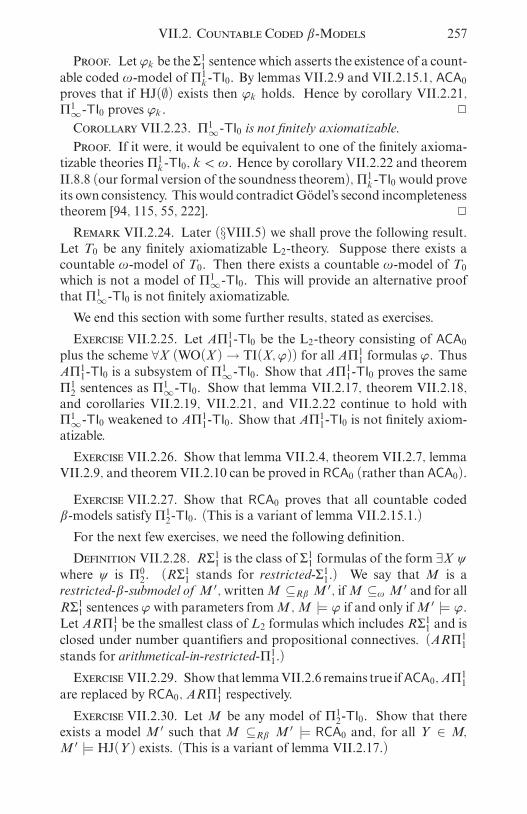
i

i

i

i

i

i

i

i


Proof. Let ϕk be the Σ11 sentence which asserts the existence of a count-

able coded ù-model of Π1k-TI0. By lemmas VII.2.9 and VII.2.15.1, ACA0

proves that if HJ(∅) exists then ϕk holds. Hence by corollary VII.2.21,Π1∞-TI0 proves ϕk . 2

Corollary VII.2.23. Π1∞-TI0 is not finitely axiomatizable.

Proof. If it were, it would be equivalent to one of the finitely axioma-tizable theories Π1k-TI0, k < ù. Hence by corollary VII.2.22 and theoremII.8.8 (our formal version of the soundness theorem), Π1k-TI0 would proveits own consistency. This would contradictGodel’s second incompletenesstheorem [94, 115, 55, 222]. 2

Remark VII.2.24. Later (§VIII.5) we shall prove the following result.Let T0 be any finitely axiomatizable L2-theory. Suppose there exists acountable ù-model of T0. Then there exists a countable ù-model of T0which is not a model of Π1∞-TI0. This will provide an alternative proofthat Π1∞-TI0 is not finitely axiomatizable.

We end this section with some further results, stated as exercises.

Exercise VII.2.25. Let AΠ11-TI0 be the L2-theory consisting of ACA0

plus the scheme ∀X (WO(X )→ TI(X,ϕ)) for all AΠ11 formulas ϕ. ThusAΠ11-TI0 is a subsystem of Π1∞-TI0. Show that AΠ11-TI0 proves the sameΠ12 sentences as Π

1∞-TI0. Show that lemma VII.2.17, theorem VII.2.18,

and corollaries VII.2.19, VII.2.21, and VII.2.22 continue to hold withΠ1∞-TI0 weakened to AΠ11-TI0. Show that AΠ11-TI0 is not finitely axiom-atizable.

Exercise VII.2.26. Show that lemma VII.2.4, theorem VII.2.7, lemmaVII.2.9, and theorem VII.2.10 can be proved in RCA0 (rather than ACA0).

Exercise VII.2.27. Show that RCA0 proves that all countable codedâ-models satisfy Π12-TI0. (This is a variant of lemma VII.2.15.1.)

For the next few exercises, we need the following definition.

Definition VII.2.28. RΣ11 is the class of Σ11 formulas of the form ∃X ø

where ø is Π02. (RΣ11 stands for restricted-Σ

11.) We say that M is a

restricted-â-submodel of M ′, writtenM ⊆Râ M ′, ifM ⊆ù M ′ and for allRΣ11 sentences ϕ with parameters fromM ,M |= ϕ if and only ifM ′ |= ϕ.Let ARΠ11 be the smallest class of L2 formulas which includes RΣ

11 and is

closed under number quantifiers and propositional connectives. (ARΠ11stands for arithmetical-in-restricted-Π11.)

Exercise VII.2.29. Show that lemmaVII.2.6 remains true ifACA0,AΠ11are replaced by RCA0, ARΠ

11 respectively.

Exercise VII.2.30. Let M be any model of Π12-TI0. Show that thereexists a model M ′ such that M ⊆Râ M ′ |= RCA0 and, for all Y ∈ M,M ′ |= HJ(Y ) exists. (This is a variant of lemma VII.2.17.)

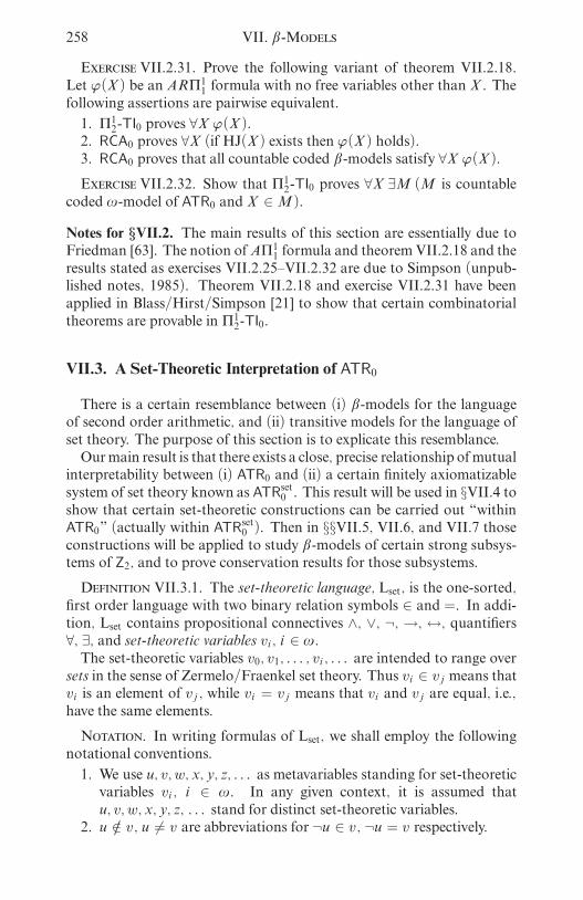
i

i

i

i

i

i

i

i

258 VII. â-Models

Exercise VII.2.31. Prove the following variant of theorem VII.2.18.Let ϕ(X ) be an ARΠ11 formula with no free variables other than X . Thefollowing assertions are pairwise equivalent.

1. Π12-TI0 proves ∀X ϕ(X ).2. RCA0 proves ∀X (if HJ(X ) exists then ϕ(X ) holds).3. RCA0 proves that all countable coded â-models satisfy ∀X ϕ(X ).Exercise VII.2.32. Show that Π12-TI0 proves ∀X ∃M (M is countablecoded ù-model of ATR0 and X ∈M ).

Notes for §VII.2. The main results of this section are essentially due toFriedman [63]. The notion ofAΠ11 formula and theoremVII.2.18 and theresults stated as exercises VII.2.25–VII.2.32 are due to Simpson (unpub-lished notes, 1985). Theorem VII.2.18 and exercise VII.2.31 have beenapplied in Blass/Hirst/Simpson [21] to show that certain combinatorialtheorems are provable in Π12-TI0.

VII.3. A Set-Theoretic Interpretation of ATR0

There is a certain resemblance between (i) â-models for the languageof second order arithmetic, and (ii) transitive models for the language ofset theory. The purpose of this section is to explicate this resemblance.Ourmain result is that there exists a close, precise relationship ofmutualinterpretability between (i) ATR0 and (ii) a certain finitely axiomatizablesystem of set theory known as ATR

set0 . This result will be used in §VII.4 to

show that certain set-theoretic constructions can be carried out “withinATR0” (actually within ATR

set0 ). Then in §§VII.5, VII.6, and VII.7 those

constructions will be applied to study â-models of certain strong subsys-tems of Z2, and to prove conservation results for those subsystems.

Definition VII.3.1. The set-theoretic language, Lset, is the one-sorted,first order language with two binary relation symbols ∈ and =. In addi-tion, Lset contains propositional connectives ∧, ∨, ¬, →, ↔, quantifiers∀, ∃, and set-theoretic variables vi , i ∈ ù.The set-theoretic variables v0, v1, . . . , vi , . . . are intended to range oversets in the sense of Zermelo/Fraenkel set theory. Thus vi ∈ vj means thatvi is an element of vj , while vi = vj means that vi and vj are equal, i.e.,have the same elements.

Notation. In writing formulas of Lset, we shall employ the followingnotational conventions.

1. We use u, v,w, x, y, z, . . . as metavariables standing for set-theoreticvariables vi , i ∈ ù. In any given context, it is assumed thatu, v,w, x, y, z, . . . stand for distinct set-theoretic variables.

2. u /∈ v, u 6= v are abbreviations for ¬u ∈ v, ¬u = v respectively.

i

i

i

i

i

i

i

i

VII.3. A Set-Theoretic Interpretation of ATR0 259

3. ∅ = the empty set = the unique set u such that ∀x (x /∈ u). (We shallhave axioms which imply the existence and uniqueness of ∅.)

4. x : ϕ(x) = the unique set u such that ∀x (x ∈ u ↔ ϕ(x)), ifsuch a set u exists; x : ϕ(x) = ∅ otherwise. Here ϕ(x) is anyformula of Lset, and u is a variable which does not occur freely inϕ. Thus x : ϕ(x) behaves as a term. If ϕ(x) has free variablesother than x, then the term x : ϕ(x) also has those free variables.The set (denoted by the term) x : ϕ(x) is said to exist properly if∃u ∀x (x ∈ u ↔ ϕ(x)).

5. t : ϕ = y : ∃x1 · · · ∃xn (y = t ∧ ϕ). Here t is any term, ϕ is anyformula, y is a variable which does not occur freely in t or ϕ, andx1, . . . , xn are exactly the variables which do occur freely in t.

Definition VII.3.2 (abbreviated terms). Within Lset we use the follow-ing abbreviated terms.

1.⋃u = y : ∃x (y ∈ x ∧ x ∈ u) (union).

2. u, v = x : x = u ∨ x = v (unordered pair).3. u − v = x : x ∈ u ∧ x /∈ v (complement).4. u ∩ v = u − (u − v) (intersection).5. u ∪ v = ⋃u, v (union).6. x = x, x (singleton).7. 〈y, x〉 = y, x, x (ordered pair).8. v × u = 〈y, x〉 : y ∈ v ∧ x ∈ u (Cartesian product).9. dom(w) = x : ∃y (〈y, x〉 ∈ w) (domain).10. rng(w) = y : ∃x (〈y, x〉 ∈ w) (range).11. field(w) = dom(w) ∪ rng(w) (field).12. w−1 = 〈x, y〉 : 〈y, x〉 ∈ w (inverse).13. w ′x = the unique y such that 〈y, x〉 ∈ w, if such a y exists;w ′x = ∅ otherwise (value of w at x).

14. wu = w ∩ (rng(w)× u) (restriction).15. w ′′u = rng(wu) (range of the restriction).16. ∈u = 〈y, x〉 : y ∈ x ∧ x ∈ u.

Definition VII.3.3. Bset0 is a finitely axiomatized theory in the languageLset. The four axioms of Bset0 are as follows.

1. Axiom of Equality: ∀u ∀v ∀w (u = u ∧ (u = v → v = u) ∧((u = v ∧ v = w) → u = w) ∧ ((u = v ∧ v ∈ w) → u ∈ w) ∧((u ∈ v ∧ v = w)→ u ∈ w)).

2. Axiom of Extensionality: ∀u ∀v (∀x (x ∈ u ↔ x ∈ v)→ u = v).3. Axiom of Infinity: ∃u (∅ ∈ u ∧∀x ∀y ((x ∈ u ∧ y ∈ u)→ x ∪ y ∈u).

4. Axiom of Rudimentary Closure: We have an axiom which asserts,for all u, v and w, the proper existence of u, v, u − v, u × v, ⋃ u,

i

i

i

i

i

i

i

i

260 VII. â-Models

∈u, dom(w), w−1, and

〈y, 〈x, z〉〉 : 〈y, x〉 ∈ w ∧ z ∈ u,〈y, 〈z, x〉〉 : 〈y, x〉 ∈ w ∧ z ∈ u,v : ∃x (x ∈ u ∧ v = w ′′x).

Definition VII.3.4 (Σsetk formulas). The class of ∆set0 formulas of Lset is

defined inductively as follows. The formulas u = v, u 6= v, u ∈ v, u /∈ vare ∆set0 . If ϕ andø are ∆

set0 then so areϕ∧ø andϕ∨ø. If ϕ is ∆set0 then so

are ∀u (u ∈ v → ϕ) and ∃u (u ∈ v∧ϕ). The quantifiers ∀u (u ∈ v → · · · )and ∃u (u ∈ v ∧ · · · ) are known as bounded set-theoretic quantifiers.For k < ù, a formula of Lset is called Σsetk (respectively Π

setk formula) if

it is of the form ∃u1 ∀u2 · · ·uk ϕ (respectively ∀u1 ∃u2 · · ·uk ϕ) where ϕ is∆set0 . (This hierarchy of formulas will play an important role in §VII.5.)Lemma VII.3.5 (∆set0 comprehension). The scheme of ∆

set0 comprehen-

sion is provable in Bset0 . In other words, Bset0 proves

∀u ∃v ∀x (x ∈ v ↔ (x ∈ u ∧ ϕ(x)))where ϕ(x) is any∆set0 formula and v is a variable which does not ocur freelyin ϕ(x).

Proof. See Jensen [131, §1]. Alternatively, change the definition of Bset0so as to include the ∆set0 comprehension scheme. (It is not then obviousthat Bset0 is finitely axiomatizable. However, this will not matter.) 2

Definition VII.3.6 (abbreviated formulas). Within Bset0 we use the fol-lowing abbreviated formulas.

1. u ⊆ v ↔ u is a subset of v, i.e., ∀x (x ∈ u → x ∈ v).2. Rel(r)↔ r is a relation, i.e., r ⊆ rng(r)× dom(r).3. Fcn(f) ↔ f is a function, i.e., Rel(f) ∧ ∀x ∀y ∀z ((〈y, x〉 ∈ f ∧

〈z, x〉 ∈ f)→ y = z).4. Inj(f) ↔ f is an injection, i.e., Fcn(f) ∧ ∀x ∀y ∀z ((〈z, x〉 ∈ f ∧

〈z, y〉 ∈ f)→ x = y).5. u ≈ v ↔ u and v are equinumerous, i.e., ∃f (Inj(f)∧dom(f) = u∧rng(f) = v).

6. Trans(u)↔ u is transitive, i.e., ∀x ∀y ((x ∈ y ∧ y ∈ u)→ x ∈ u).7. Ord(u)↔ u is an ordinal, i.e., Trans(u)∧ ∀x ∀y ((x ∈ u ∧ y ∈ u)→(x ∈ y ∨ x = y ∨ y ∈ x)) ∧ ∀v ((v ⊆ u ∧ v 6= ∅) → ∃x (x ∈ v ∧∀y (y ∈ v → y /∈ x))).

8. Succ(u)↔ u is a successor ordinal, i.e., Ord(u) ∧ ∃v (u = v ∪ v).9. Lim(u)↔ u is a limit ordinal, i.e., Ord(u) ∧ u 6= ∅ ∧ ¬Succ(u).10. FinOrd(u)↔ u is a finite ordinal, i.e., Ord(u) ∧ ∀v (v ∈ u ∪ u →(v = ∅ ∨ Succ(v))).

11. Fin(u)↔ u is finite, i.e., ∃v (u ≈ v ∧ FinOrd(v)).12. HFin(u) ↔ u is hereditarily finite, i.e., ∃v (u ⊆ v ∧ Trans(v) ∧Fin(v)).

i

i

i

i

i

i

i

i


13. Ctbl(u) ↔ u is countable, i.e., ∃f (Inj(f) ∧ dom(f) = u ∧ ∀y(y ∈ rng(f)→ FinOrd(y))).

14. HCtbl(u)↔ u is hereditarily countable, i.e., ∃v (u ⊆ v ∧ Trans(v) ∧Ctbl(v)).

We use α, â, ã, ä, . . . as special variables ranging over ordinals. We usei, j, k,m, n, . . . as special variables ranging over finite ordinals. We write0 = ∅, 1 = 0, 2 = 0, 1, . . . ; α + 1 = α ∪ α; α < â ↔ α ∈ â ;α ≤ â ↔ (α < â ∨α = â); ù = m : FinOrd(m); HF = u : HFin(u).Lemma VII.3.7. The following facts are provable in Bset0 .

1. ¬α < α; α = â : â < α.2. (α < â ∧ â < ã)→ α < ã.3. α < â ∨ α = â ∨ â < α.4. Ord(α + 1); ∀â (â < α + 1↔ â ≤ α).5. (Lim(â) ∧ α < â)→ α + 1 < â .6. Lim(ù); ∀α (α < ù ↔ Fin(α)).7. Let z be a nonempty set of ordinals. Then: (i) z has a least element;(ii)⋃z is an ordinal; (iii)

⋃z is the least upper bound of z.

8. u ≈ u; u ≈ v → v ≈ u; (u ≈ v ∧ v ≈ w)→ u ≈ w.9. ∅ ≈ 0; (u ≈ m ∧ x /∈ u)→ u ∪ x ≈ m + 1.10. (u ≈ m ∧ v ≈ n ∧ u ⊆ v)→ m ≤ n.11. m ≈ n ↔ m = n.12. Fin(u)↔ ∃m (u ≈ m).13. Fin(∅); Fin(x)→ Fin(x ∪ y).14. (u ⊆ v ∧ Fin(v))→ Fin(u).15. (Fin(u) ∧ Fin(v))→ (Fin(u ∪ v) ∧ Fin(u × v)).16. (Fin(u) ∧ ∀v (v ∈ u → Fin(v)))→ Fin(⋃ u).17. (∀v (v ∈ w → v ⊆ u) ∧ Trans(u))→ Trans(u ∪ w).18. The setHF = u : HFin(u) exists properly.19. u ∈ HF↔ (Fin(u) ∧ u ⊆ HF).Proof. The proof is straightforward using lemma VII.3.5. 2

We are now ready to define the theory ATRset0 .

Definition VII.3.8. ATRset0 is a finitely axiomatized theory in the set-

theoretic language Lset. The axioms of ATRset0 are those of B

set0 plus the

following three:

1. Axiom of Regularity:

∀u (u 6= ∅ → ∃x (x ∈ u ∧ ∀y (y ∈ u → y /∈ x))).2. Axiom of Countability: ∀u (u is hereditarily countable).3. Axiom Beta: A relation r is said to be regular if

∀u (u 6= ∅ → ∃x (x ∈ u ∧ ∀y (y ∈ u → 〈y, x〉 /∈ r))).The axiom asserts that, for all regular relations r, there exists afunction f such that dom(f) = field(r) and, for all x ∈ field(r),

i

i

i

i

i

i

i

i

262 VII. â-Models

f′x = f′′y : 〈y, x〉 ∈ r. This f is called the collapsing functionof r.

It can be shown (in ZF, for instance) that the hereditarily countable setsform a transitive model of ATR

set0 .

We shall see that there is a canonical one-to-one correspondence be-tween transitive models of ATR

set0 and â-models of ATR0. This is a special

case of a more general canonical one-to-one correspondence between ar-bitrary models of ATR

set0 and arbitrary models of ATR0. We now give one

direction of the more general correspondence.

Theorem VII.3.9. Each axiom of ATR0 is, in its natural translation, atheorem of ATR

set0 .

Proof. The natural translation of L2 into Lset is defined as follows.Then number variables of L2 are interpreted in Lset as ranging over finiteordinals, i.e., elements of ù. The set variables of L2 are interpreted inLset as ranging over subsets of ù. Using lemma VII.3.5 and parts 11, 12and 15 of lemma VII.3.7, Bset0 proves the existence of functions +, · withdom(+) = dom(·) = ù × ù where m + n = the unique k ∈ ù such that(m×0)∪(n×1) ≈ k,m ·n = the unique k ∈ ù such thatm×n ≈ k.The symbols +, ·, 0, 1, <, =, ∈ of L2 are then interpreted by means oftheir obvious counterparts over ù in Lset. By lemmas VII.3.5 and VII.3.7it is clear that each axiom of ACA0 becomes, under the above translation,a theorem of Bset0 .Without comment, we shall from now on identify formulas of L2 withtheir translations into Lset as given above.It remains to show that the principal axiom of ATR0 is a theorem of

ATRset0 . As in §V.6, let CWO be the assertion of comparability of countable

well orderings, i.e.,

∀X ∀Y ((WO(X ) ∧WO(Y ))→ (|X | ≤ |Y | ∨ |X | ≥ |Y |)).By theorem V.6.8 it suffices to show that CWO is a theorem of ATR

set0 .

We reason within ATRset0 . Let X,Y ⊆ ù be (codes for) countable well

orderings, i.e., assumeWO(X ) andWO(Y ). Set rX = 〈n,m〉 : n <X m.Then rX is a regular relation, so by Axiom Beta let fX be the collapsingfunction of rX , i.e., dom(fX ) = field(rX ) and f′

Xm = f′′n : 〈n,m〉 ∈

rX for all m ∈ field(rX ). Put αX = rng(fX ). It is easy to check that αXis an ordinal, the order type of X , and thatfX is the unique isomorphismof X with αX . Similarly define rY and let fY be the unique isomorphismofY with its order type αY . By part 3 of VII.3.7, we have either αX ≤ αYor αY ≤ αX . Suppose for definiteness that αX ≤ αY . Put

g = (m, n) : m ∈ field(X ) ∧ n ∈ field(Y ) ∧ f′Xm = f

′Yn.

Then clearly g : |X | ≤ |Y |. Similarly if αY ≤ αX we have g : |X | ≥ |Y |.This completes the proof. 2

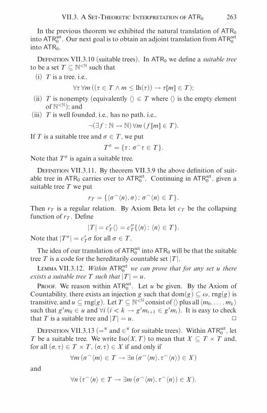
i

i

i

i

i

i

i

i


In the previous theorem we exhibited the natural translation of ATR0

into ATRset0 . Our next goal is to obtain an adjoint translation from ATR

set0

into ATR0.

Definition VII.3.10 (suitable trees). In ATR0 we define a suitable treeto be a set T ⊆ N<N such that

(i) T is a tree, i.e.,

∀ô ∀m ((ô ∈ T ∧m ≤ lh(ô))→ ô[m] ∈ T );(ii) T is nonempty (equivalently 〈〉 ∈ T where 〈〉 is the empty elementof N<N); and

(iii) T is well founded, i.e., has no path, i.e.,

¬(∃f : N → N)∀m (f[m] ∈ T ).If T is a suitable tree and ó ∈ T , we put

T ó = ô : óaô ∈ T.Note that T ó is again a suitable tree.

Definition VII.3.11. By theorem VII.3.9 the above definition of suit-able tree in ATR0 carries over to ATR

set0 . Continuing in ATR

set0 , given a

suitable tree T we put

rT = 〈óa〈n〉, ó〉 : óa〈n〉 ∈ T.Then rT is a regular relation. By Axiom Beta let cT be the collapsingfunction of rT . Define

|T | = c′T 〈〉 = c′′T〈n〉 : 〈n〉 ∈ T.Note that |T ó | = c′Tó for all ó ∈ T .The idea of our translation of ATR

set0 into ATR0 will be that the suitable

tree T is a code for the hereditarily countable set |T |.Lemma VII.3.12. Within ATR

set0 we can prove that for any set u there

exists a suitable tree T such that |T | = u.Proof. We reason within ATR

set0 . Let u be given. By the Axiom of

Countability, there exists an injection g such that dom(g) ⊆ ù, rng(g) istransitive, and u ⊆ rng(g). LetT ⊆ N<N consist of 〈〉plus all 〈m0, . . . , mk〉such that g ′m0 ∈ u and ∀i (i < k → g ′mi+1 ∈ g ′mi). It is easy to checkthat T is a suitable tree and |T | = u. 2

Definition VII.3.13 (=∗ and ∈∗ for suitable trees). Within ATRset0 , let

T be a suitable tree. We write Iso(X,T ) to mean that X ⊆ T × T and,for all (ó, ô) ∈ T × T , (ó, ô) ∈ X if and only if

∀m (óa〈m〉 ∈ T → ∃n (óa〈m〉, ôa〈n〉) ∈ X )and

∀n (ôa〈n〉 ∈ T → ∃m (óa〈m〉, ôa〈n〉) ∈ X ).

i

i

i

i

i

i

i

i

264 VII. â-Models

If S and T are suitable trees, we define S ⊕ T to be the suitable treeconsisting of 〈〉 plus all 〈0〉aó and 〈1〉aô such that ó ∈ S and ô ∈ T . Wedefine

S =∗ T ↔ ∃X (Iso(X,S ⊕ T ) ∧ (〈0〉, 〈1〉) ∈ X ))and

S ∈∗ T ↔ ∃X (Iso(X,S ⊕ T ) ∧ ∃n (〈0〉, 〈1, n〉) ∈ X )).Lemma VII.3.14. Within ATR

set0 we can prove that, for all suitable trees

S and T ,

S =∗ T ↔ |S| = |T |,and

S ∈∗ T ↔ |S| ∈ |T |.Proof. Given a suitable tree T , put

X = (ó, ô) : ó ∈ T ∧ ô ∈ T ∧ c′Tó = c′T ô.Then clearly X is the unique set such that Iso(X,T ). Applying this to thesuitable tree S ⊕ T instead of T , we obtain the desired conclusions. 2

Definition VII.3.15. Let Vi , i ∈ ù be fixed distinct set variables of L2.We shall use these variables to denote suitable trees. We shall link Vi tothe set-theoretic variable vi (cf. definition VII.3.1). To each formula ϕ ofLset, we associate a formula |ϕ| of L2 as follows.

|vi = vj | is Vi =∗ Vj ;|vi ∈ vj | is Vi ∈∗ Vj ;

|¬ϕ| is ¬|ϕ|; |ϕ ∧ø| is |ϕ| ∧ |ø|; etc.;|∀vi ϕ| is ∀Vi (Vi suitable→ |ϕ|);|∃vi ϕ| is ∃Vi (Vi suitable ∧ |ϕ|).

Note that if vi1 , . . . , vik are the free variables of ϕ, then Vi1 , . . . , Vik are thefree variables of |ϕ|.Lemma VII.3.16. Let ϕ be any formula of Lset. Let vi1 , . . . , vik be thefree variables ofϕ. ThenATR

set0 proves the following. For all sets vi1 , . . . , vik

and all suitable trees Vi1 , . . . , Vik such that |Vi1 | = vi1 , . . . , |Vik | = vik , wehave ϕ ↔ |ϕ|. In particular, ATR

set0 proves ϕ ↔ |ϕ| for all sentences ϕ of

Lset.

Proof. This follows by a straightforward induction on the number ofsymbols in ϕ, using lemmas VII.3.14 and VII.3.12. 2

Our next task is to show that the set-theoretic properties of suitabletrees can be proved in ATR0.

i

i

i

i

i

i

i

i


Lemma VII.3.17. The following is provable in ATR0. Let T be a suitabletree. Then there exists a unique set X such that Iso(X,T ). Furthermore,for all ó ∈ T and ô ∈ T , we have

T ó =∗ T ô ↔ (ó, ô) ∈ Xand

T ó ∈∗ T ô ↔ ∃n ((ó, ôa〈n〉) ∈ X ).In particular, X is an equivalence relation on T .

Proof. The existence of X is proved by arithmetical transfinite recur-sion along (theKleene/Brouwer ordering of)T . The uniqueness is provedby arithmetical transfinite induction. The rest is straightforward using thefact that, for each ñ ∈ T , if we define

X ñ = (ó, ô) : (ñaó, ñaô) ∈ Xthen Iso(X ñ, T ñ) holds. 2

Definition VII.3.18. In ATR0, for X ⊆ N we define X∗ to be thesuitable tree consisting of 〈〉 and all 〈m0, . . . , mk〉 such that m0 ∈ Xand ∀i (i < k → mi+1 < mi). For n ∈ N we define n∗ = X∗ whereX = 0, . . . , n − 1.The point of the previous definition is that, provably in ATR

set0 , |X∗| =

X and |n∗| = n. Thus n ∈ X if and only if n∗ ∈∗ X∗. This is a specialcase of:

Lemma VII.3.19. Let ϕ be any formula of L2. LetX1, . . . , Xi , n1, . . . , njbe the free variables of ϕ. Then ATR0 proves the following. For all suitabletrees V1, . . . , Vi , Vi+1, . . . , Vi+j such that V1 =∗ X∗

1 , . . . , Vi =∗ X∗

i ,Vi+1 =∗ n∗1 , . . . , Vi+j =∗ n∗j , we have ϕ ↔ |ϕ|.Proof. The proof is by a straightforward induction on the number ofsymbols in ϕ. We omit the details. 2

Lemma VII.3.20. Let ϕ be any one of the axioms of ATRset0 . Then |ϕ| is

a theorem of ATR0.

Proof. We reasonwithinATR0. The proofs of |Axiom of Equality| and|Axiom of Extensionality| are straightforward, using lemma VII.3.17.In order to handle the Axiom of Rudimentary Closure, we constructappropriate suitable trees. For example, given suitable trees V0 and V1,we can construct a suitable tree

V2 = V0 ⊕ V1 = 〈〉 ∪ 〈0〉aô : ô ∈ V0 ∪ 〈1〉aô : ô ∈ V1.It is then straightforward to prove that for all suitable trees V3,

V3 ∈∗ V2 ↔ (V3 =∗ V0 ∨ V3 =∗ V1)i.e., |∀v3 (v3 ∈ v2 ↔ (v3 = v0 ∨ v3 = v1)|. This shows that

|∀v0 ∀v1 ∃v2∀v3 (v3 ∈ v2 ↔ (v3 = v0 ∨ v3 = v1))|,

i

i

i

i

i

i

i

i

266 VII. â-Models

i.e., |∀v0 ∀v1 ∃ v0, v1|. The other parts of |Rudimentary Closure| areproved similarly.In order to dispose of the Axiom of Infinity, we construct a suitable treeV0 in accordance with the usual coding of the hereditarily finite sets. PutnEm if and only if n occurs as an exponent in the binary expansion of m,i.e., if n = mi for some i where

m = 2m1 + 2m2 + · · ·+ 2mj , m1 > m2 > · · · > mj .We then let V0 be the suitable tree consisting of 〈〉 plus all 〈n0, . . . , nk〉such that ni+1Eni for all i < k. With this V0 it is straightforward to prove

|∅ ∈ v0 ∧ ∀v1 ∀v2 ((v1 ∈ v0 ∧ v2 ∈ v0)→ v1 ∪ v2 ∈ v0)|,hence |Axiom of Infinity|. We could also prove |v0 = HF|, but this is notneeded.We now prove |Axiom of Regularity|. Let V0 be a suitable tree suchthat |v0 6= ∅|, i.e., ∃m (〈m〉 ∈ V0). By lemma VII.3.17 let X0 be such thatIso(X0, V0). Suppose for a contradiction that

|∀v1 (v1 ∈ v0 → ∃v2 (v2 ∈ v0 ∧ v2 ∈ v1))|.By lemma VII.3.17 this is equivalent to

∀m (〈m〉 ∈ V0 → ∃n ∃j ((〈n〉, 〈m, j〉) ∈ X0)).Define f : N → N by recursion as follows. Put f(0) = the least m suchthat 〈m〉 ∈ V0. Given f[k + 1] = 〈f(0), . . . , f(k)〉, put f(k + 1) =the least j such that ∃n ((〈n〉, f[k]a〈j〉) ∈ X0). Then ∀k (f[k] ∈ V0)contradicting the well foundedness of V0.The remaining two axioms involve ordered pairs. Note that |〈vi , vj〉 =vk| is equivalent to

(Vi ⊕ Vj)⊕ (Vj ⊕ Vj) =∗ Vk .To prove |Axiom Beta|, let V0 be a given suitable tree such that

|v0 is a regular relation|.Let X be the set of all 〈k, i,m〉 such that 〈k, i,m〉 ∈ V0. Let V1 consist of〈〉 plus all 〈ó〉aô such that ó ∈ X and ô ∈ V ó0 . It is easy to check that V1is a suitable tree, and that

∣∣∣v1 =⋃⋃⋃

v0 = field(v0)∣∣∣ .

Now by lemma VII.3.17 let X0 be such that Iso(X0, V0). Let R be theset of all (ó, ô) ∈ X × X such that for some i, j, k,m, n, p and p we have(ô, 〈k, i, n〉) ∈ X0, (ó, ô) /∈ X0, (〈k, i〉, 〈k, j〉) /∈ X0, (ó, 〈k, j, p〉) ∈ X0. LetV2 consist of 〈〉 plus all 〈ó0, . . . , ók〉 such that ∀i (i < k → (ói , ói+1) ∈ R).Let V3 consist of 〈〉 plus all 〈ó〉aô such that ó ∈ X and

ô ∈ (V 〈ó〉2 ⊕ V ó0 )⊕ (V ó0 ⊕ V ó0 ).

i

i

i

i

i

i

i

i


It is straightforward to check that V2 and V3 are suitable trees, and that

|v2 = rng(v3) where v3 is the collapsing function of v0|.It remains to prove |Axiom of Countability|. Let V0 be a given suitabletree. We may regard each ó ∈ V0 ⊆ N as an element of N and form thecorresponding suitable tree ó∗ as in definition VII.3.18. Let V1 consist of〈〉 plus all 〈ó〉aô such that ó ∈ V0 and ô ∈ (V ó0 ⊕ ó∗)⊕ (ó∗ ⊕ ó∗). It isstraightforward to check that |Fcn(v1)∧dom(v1) ⊆ ù∧Trans(rng(v1))∧v0 ⊆ rng(v1)|.This completes the proof of lemma VII.3.20. 2

Exercise VII.3.21. Show that ATRset0 proves, for all sets v, the proper

existence of

TC(v) =⋃⋃n

v : n ∈ ù

where⋃0v = v and

⋃n+1v =

⋃⋃nv for all n ∈ ù. Also, ATR

set0 proves

that TC(v) is the smallest transitive set u such that v ⊆ u. TC(v) is knownas the transitive closure of v.

We are now ready to deduce the main results of this section.

Theorem VII.3.22. Let ϕ be a sentence of Lset. Then ATRset0 proves ϕ if

and only if ATR0 proves |ϕ|.Proof. Suppose first thatATR

set0 provesϕ. By lemmaVII.3.20 it follows

thatATR0 proves |ϕ|. Conversely, suppose thatATR0 proves |ϕ|. It followsby theorem VII.3.9 that ATR

set0 proves |ϕ|. But then by lemma VII.3.16 it

follows that ATRset0 proves ϕ. 2

Theorem VII.3.23 (a conservation theorem). ATRset0 is a conservative

extension of ATR0. In other words, for any sentence ϕ of L2, ATRset0 proves

ϕ if and only if ATR0 proves ϕ.

Proof. By theoremVII.3.22,ATRset0 provesϕ if and only ifATR0 proves

|ϕ|. But by lemma VII.3.19 ATR0 proves |ϕ| ↔ ϕ, so the desired conclu-sion follows. 2

For use in §§VII.4 and VII.5, we prove the following theorem whichrelates the set-theoretic hierarchy Σsetk , k < ù (definition VII.3.4) to theprojective hierarchy Σ1k+1, k < ù (definition I.5.1).

Theorem VII.3.24. Assume 0 ≤ k < ù.1. If ϕ is a Σsetk formula ofLset, then |ϕ| is equivalent (provably in ATR

set0 )

to a Σ1k+1 formula of L2.

2. Conversely, each Σ1k+2 formula of L2 is equivalent (provably in ATRset0 )

to a Σsetk+1 formula of Lset.

Proof. We first show by induction on ∆set0 formulas ϕ that |ϕ| is equiv-alent to a Σ11 formula. By definitions VII.3.15 and VII.3.13, |vi = vj | and

i

i

i

i

i

i

i

i

268 VII. â-Models

|vi ∈ vj | are equivalent to the Σ11 formulas∃X (Iso(X,Vi ⊕ Vj) ∧ (〈0〉, 〈1〉) ∈ X )

and

∃X (Iso(X,Vi ⊕ Vj) ∧ ∃n ((〈0〉, 〈1, n〉) ∈ X ))respectively. Hence, by lemmas VII.3.9 and VII.3.17, |vi 6= vj | and|vi /∈ vj | are equivalent to the Σ11 formulas

∃X (Iso(X,Vi ⊕ Vj) ∧ (〈0〉, 〈1〉) /∈ X )and

∃X (Iso(X,Vi ⊕ Vj) ∧ ∀n (〈0〉, 〈1, n〉) /∈ X )respectively. It is also clear that if |ϕ| and |ø| are Σ11, then so are |ϕ| ∧ |ø|and |ϕ| ∨ |ø|, i.e., |ϕ ∧ ø| and |ϕ ∨ ø|. Finally, by lemma VII.3.17,|∀vi (vi ∈ vj → ϕ)| and |∃vi (vi ∈ vj ∧ ϕ)| are equivalent to

∀n (〈n〉 ∈ Vj → ∃Vi (Vi =∗ V 〈n〉j ∧ |ϕ|))

and

∃n (〈n〉 ∈ Vj ∧ ∃Vi (Vi =∗ V 〈n〉j ∧ |ϕ|))

respectively. These formulas are Σ11 if |ϕ| is. At this point we are using theΣ11 axiom of choice, a consequence of ATR0 (theorem V.8.3).So far we have shown that ϕ Σset0 implies |ϕ| Σ11. Suppose now that ϕ isΣsetk+1, say ∃vi ø where ø is Πsetk . By induction on k, |ø| is Π1k+1. Hence|ϕ|, i.e.,

∃Vi (Vi suitable ∧ |ø|),is Σ1k+2. This completes the proof of part 1.

We now prove the converse. Let ϕ be a Σ12 formula of L2. By lemmaV.1.4 (the Kleene normal form theorem), we can write ϕ in the form

∃X ∀f ∃n ¬è(X,f[n])where è is arithmetical. We may also assume that è(X,f[n]) impliesè(X,f[m]) for all m ≤ n. Thus ∀f ∃n ¬è(X,f[n]) is equivalent to regu-larity of the relation 〈ôa〈k〉, ô〉 : è(X, ôa〈k〉). By Axiom Beta and theAxiom of Regularity, this is equivalent to the existence of an appropriatecollapsing function. Thus ϕ is equivalent to the Σset1 formula

∃X ∃g (Fcn(g) ∧ ∀ô ∀k (è(X, ôa〈k〉)→ g ′ôa〈k〉 ∈ g ′ô)).The previous paragraph shows that every Σ12 formula of L2 is equivalentto a Σset1 formula of Lset. It follows easily that every Σ

1k+2 formula of L2 is

equivalent to a Σsetk+1 formula of Lset.This completes the proof of theorem VII.3.24. 2

i

i

i

i

i

i

i

i


Theorems VII.3.22 and VII.3.23 established a close and precise rela-tionship of mutual interpretability between ATR0 (a subsystem of secondorder arithmetic) and ATR

set0 (a system of set theory). We shall now

reformulate these results in model-theoretic terms.

Definition VII.3.25.

1. A model for Lset or Lset-structure is an ordered pair

A = (|A|,∈A)where |A| is a nonempty set and ∈A⊆ |A| × |A| is a binary relationon |A|.

2. Let ϕ be a sentence of Lset with parameters from |A|. We say thatAsatisfies ϕ or is a model of ϕ, written A |= ϕ, if ϕ is true when thevariables are interpreted as ranging over |A|, ∈ is interpreted as ∈A,= is interpreted as

=A = 〈a, a〉 : a ∈ |A|,and the parameters are interpreted as themselves.

3. The model A is said to be well founded if there is no infinite sequence〈an : n < ù〉 such that an+1 ∈A an for all n < ù.

4. The model A is said to be transitive if |A| is a transitive set and∈A = ∈|A|.

It can be shown (in ZF, for instance) that any transitive Lset-structuresatisfies the Axiom of Extensionality and is well founded. Conversely, anywell founded Lset-structure which satisfies the Axiom of Extensionality isuniquely isomorphic to a transitive model.

Definition VII.3.26. To any model A = (|A|,∈A) of Bset0 we canoni-cally associate a model

A2 =M = (|M |,SM ,+M , ·M , 0M , 1M , <M )of ACA0. Namely |M | = a ∈ |A| : A |= FinOrd(a); SM = bA : A |=b ⊆ ù where bA = a ∈ |A| : A |= a ∈ b; and +M , ·M , 0M , 1M , <Mare defined in the natural way (cf. the proof of theorem VII.3.9).

Theorem VII.3.27. Let A be a model of ATRset0 . Then:

1. A2 is a model of ATR0;2. A2 is a â-model if and only if A is well founded.

Proof. Part 1 is an immediate consequence of theorem VII.3.9. Part 2follows easily. 2

In the opposite direction, we have:

Definition VII.3.28. To any model

M = (|M |,SM ,+M , ·M , 0M , 1M , <M )

i

i

i

i

i

i

i

i

270 VII. â-Models

for L2 we associate a modelMset for Lset as follows. Put

TM = T ∈ SM : M |= T is a suitable treeFor T ∈ TM put

[T ] = T ′ ∈ TM : M |= T =∗ T ′and define

|A| = [T ] : T ∈ TM.For T,T ′ ∈ TM define [T ] ∈A [T ′] if and only if M |= T ∈∗ T ′. ThusA = (|A|,∈A) is a model for Lset, and we define

Mset = A = (|A|,∈A).It can be shown that ifM is model of ACA0, thenMset is a model of Bset0 .

Theorem VII.3.29. Let M be a model of ATR0. Then Mset is a modelof ATR

set0 . Furthermore (Mset)

2 = M up to a canonical isomorphism.Conversely, if A is a model of ATR

set0 , then (A

2)set = A up to a canonicalisomorphism.

Proof. This is an immediate consequence of lemmasVII.3.20, VII.3.19,VII.3.12 and VII.3.14. 2

Definition VII.3.30. Let A = (|A|,∈A) and B = (|B|,∈B ) be modelsfor Lset. We say that A is a transitive submodel of B, written A ⊆trans B, if|A| ⊆ |B| and, for all a ∈ |A| and b ∈ |B|, b ∈B a if and only if b ∈ |A|and b ∈A a.The above notion of transitive submodel (⊆trans) is similar to the notionof â-submodel (⊆â , definition VII.1.11). Thus A is transitive if and onlyif A ⊆trans the universe of ZF set theory. But in general, the models A andB in the above definition need not be transitive or even well founded.

Theorem VII.3.31. IfM ′ is a model of ATR0 andM ⊆â M ′, thenMsetis (canonically isomorphic to) a transitive submodel ofM ′

set. Conversely, ifA and B are models of ATR

set0 and A ⊆trans B, then A2 is a â-submodel

of B2.

Proof. The formula “T is a suitable tree” is Π11. Hence TM = SM ∩TM ′

and the first part of the theorem follows easily. The second part followsusing Axiom Beta in A and the Axiom of Regularity in B. 2

Combining this with theorem VII.1.19, we obtain:

Theorem VII.3.32. Let B be any countable model of ATRset0 . Then there

exists a proper transitive submodel A ⊆trans B, A 6= B, such thatA is againa model of ATR

set0 .

Proof. Theorems VII.3.27, VII.3.29 and VII.3.31 establish a canoni-cal one-to-one correspondence between models of ATR

set0 and models of

ATR0. Applying this to theoremVII.1.19, we obtain the desired result. 2

i

i

i

i

i

i

i

i


We shall now end this section by generalizing its main result so as toapply to systems of second order arithmetic which are stronger thanATR0.

Definition VII.3.33. Let T0 be any theory in the language L2 such thatATR0 ⊆ T0, i.e., each axiom of ATR0 is a theorem of T0. Define

T set0 = ATRset0 + T0,

i.e., T set0 is that theory in the language Lset whose axioms are those ofATR

set0 plus (the natural translations into Lset, as in theorem VII.3.9, of)

those of T0.

Theorem VII.3.34. Let T0 be any L2-theory which includes ATR0. Thenlemmas VII.3.12, VII.3.14, VII.3.16, VII.3.17, VII.3.19, VII.3.20 and the-orems VII.3.9, VII.3.22, VII.3.23, VII.3.24, VII.3.27, VII.3.29, VII.3.31continue to hold when ATR0 and ATR

set0 are replaced by T0 and T

set0 respec-

tively. In particular, T set0 is a conservative extension of T0. Also, for allsentences ϕ of Lset, T set0 proves ϕ if and only if T0 proves |ϕ|.For example, ifM is any L2-model, we haveM |=Π11-CA0 if and only ifMset |=Π11-CA

set0 . Note also thatM is a â-model if and only ifMset is well

founded. (Compare this with our earlier characterization of â-models ofΠ11-CA0, theorem VII.1.8.)

Proof. The results for T0 ⊇ ATR0 are all immediate corollaries of thespecial case T0 = ATR0. 2

Remark VII.3.35. Theorem VII.3.32 does not in general hold withATR

set0 replaced by T

set0 . For example, let M be the unique minimum

â-model of Π11-CA0 (corollary VII.1.8). Then by theorem VII.3.34,Msetis the unique smallest (up to canonical isomorphism) well founded modelof Π11-CA

set0 . In particular, there is no proper transitive submodel ofMset

which is again a model of Π11-CAset0 .

Exercise VII.3.36. Show that Π11-CAset0 is equivalent to ATR

set0 plus the

axiom

∀v ∃u (v ∈ u ∧ Trans(u) ∧ 〈u,∈u〉 |= ATRset0 ).

Hint: Use theorem VII.2.10.

Exercise VII.3.37. Give a characterization of Π11-TRset0 analogous to

the above characterization of Π11-CAset0 . (See exercises VII.1.17 and

VII.1.18.)

Exercise VII.3.38. Recall that Π1∞-TI0 is the L2 theory consisting ofACA0 plus the transfinite induction scheme (see §VII.2). Show that Π1∞-TIset0 is equivalent to ATR

set0 plus the ∈-induction scheme

∀x (∀y (y ∈ x → ϕ(y))→ ϕ(x))→ ∀x ϕ(x),where ϕ(x) is an arbitrary formula of Lset.

i

i

i

i

i

i

i

i

272 VII. â-Models

Exercise VII.3.39. Show that Σ12-ACset0 is equivalent to ATR

set0 plus the

scheme of Σset1 collection, i.e.,

∀x ∃y ϕ(x, y)→ ∀u ∃v ∀x (x ∈ u → ∃y (y ∈ v ∧ ϕ(x, y)))where ϕ(x, y) is any Σset1 formula and v is a variable which does not occurfreely in ϕ(x, y).

Exercise VII.3.40. Characterize T set0 when T0 is any of the followingL2-theories: Π1k+1-CA0, ∆1k+2-CA0, Π1k-TR0, Σ1k+2-AC0, Σ1k+2-DC0, Π1∞-

CA0, Σ1∞-AC0, Σ1∞-DC0. (See also §§VII.5, VII.6 and VII.7.)

Notes for §VII.3. The ideas of this section can be traced to the workof Godel [97, note 1] and Addison [4] relating the projective hierarchyto constructible sets. The fact that Axiom Beta is provable in ZF is dueto Mostowski [192]. (Note: We use ZF to denote Zermelo/Fraenkel settheory including the Axiom of Regularity but not the axiom of choice.)In this context Axiom Beta is known as theMostowski collapsing lemma.Also due to Mostowski [193] is the canonical one-to-one correspondencebetween â-models of Σ1∞-AC0 and well founded models of Bset0 plus theAxiom of Regularity plus the Axiom of Countability plus Σset∞ collection.Barwise/Fisher [14] (see also Barwise [13, §V.8]) used Axiom Beta in theiranalysis of Shoenfield’s absoluteness theorem (see also theorem VII.4.12below). See also Abramson/Sacks [3]. The system ATR

set0 and the idea

of considering Axiom Beta as an alternative to Σset1 collection are due toSimpson [234] and independently to McAloon/Ressayre [183]. The one-to-one correspondence between models of ATR0 and models of ATR

set0

is due to Simpson [234]. Theorems VII.1.19 and VII.3.32 are due toSimpson [234] in answer to a question of McAloon/Ressayre [183].

VII.4. Constructible Sets and Absoluteness

We begin this section by developing some of the basic properties ofGodel’s hierarchy of constructible sets within ATR

set0 . We then show that

someof themore advanced properties, such as the Shoenfield absolutenesstheorem, can be proved within Π11-CA

set0 .

The reader of this section is assumed to be familiar with the defini-tions and results of §VII.3 above. In addition, some previous knowledgeof constructible sets would be helpful although perhaps not absolutelyindispensable.

Lemma VII.4.1. The following is provable inATRset0 . Let u be a nonempty

transitive set. There exists a unique set def(u) consisting of all v ⊆ usuch that v is definable over the model 〈u,∈u〉 by a formula of Lset withparameters from u.

i

i

i

i

i

i

i

i

VII.4. Constructible Sets and Absoluteness 273

Proof. We reason within ATRset0 . Let u be a given nonempty transi-

tive set. By the Axiom of Countability, let g be an injection such thatdom(g) = u and rng(g) ⊆ ù.We shall employ a language Luset which consists of Lset augmented byconstant symbols denoting the elements of u. We shall identify terms andformulas with their Godel numbers. For each i < ù, we have a variable(0, i) denoted vi and intended to range over u. For each a ∈ u we have aconstant symbol (1, g′a) denoted a and intended to denote a. The termsof Luset are the variables vi , i < ù and the constant symbols a, a ∈ u. Forall terms s and t we have formulas (2, (s, t)) and (3, (s, t)) denoted s = tand s ∈ t respectively. For all formulas ϕ and ø we have formulas (4, ϕ)and (5, (ϕ,ø)) denoted ¬ϕ and ϕ ∧ ø respectively. For all formulas ϕand variables vi we have a formula (6, (vi , ϕ)) denoted ∀vi ϕ. A sentenceof Luset is a formula of L

uset with no free variables. Let S

u be the set ofsentences of Luset, and let F

u be the set of formulas of Luset with at mostone free variable. If ϕ(vi ) ∈ Fu with free variable vi , then for each a ∈ u,ϕ(a) is the sentence obtained by substituting the constant symbol a foreach free occurrence of vi .By arithmetical transfinite recursion (theorem VII.3.9), there exists avaluation f : Su → 0, 1 satisfying the following inductive clauses:

f(a = b) =

1 if a = b,

0 if a 6= b;

f(a ∈ b) =1 if a ∈ b,0 if a /∈ b;

f(¬ϕ) = 1− f(ϕ);

f(ϕ ∧ ø) =1 if f(ϕ) = f(ø) = 1,

0 otherwise;

f(∀vi ϕ(vi )) =1 if f(ϕ(a)) = 1 for all a ∈ u,0 otherwise.

By arithmetical transfinite induction, f is unique. Let Tu be the suit-able tree consisting of 〈〉 plus all 〈ϕ(vi )〉 such that ϕ(vi) ∈ Fu , plus all〈ϕ(vi ), a0, . . . , ak〉 such that ϕ(vi) ∈ Fu , f(ϕ(a0)) = 1, and f(ai+1 ∈ai) = 1 for all i < k. Then clearly |Tu | = def(u). This proves the exis-tence of def(u). The uniqueness is straightforward. (Note that, althoughwe used g to prove the existence of def(u), the set def(u) does not dependon the choice of g.) 2

Lemma VII.4.2 (the constructible hierarchy). The following is provablein ATR

set0 . Let u be a nonempty transitive set. Let ã be an ordinal. There

i

i

i

i

i

i

i

i

274 VII. â-Models

exists a unique set Luã such that

∃f (Fcn(f) ∧ dom(f) = ã + 1 ∧ f′ã = Luã

∧ f′0 = u ∧ ∀α (α < ã → f′α + 1 = def(f′α))

∧ ∀ä ((ä ≤ ã ∧ Lim(ä))→ f′ä =⋃f′′ä)).

Proof. We reason within ATRset0 . Let u be a nonempty transitive set

and let ã be an ordinal. By the Axiomof Countability, let g be an injectionsuch that dom(g) = ã ∪ u and rng(g) ⊆ ù.We shall employ a ramified language. For each i < ù and α < ã,we have a variable (0, (i, g ′α)) denoted vαi and intended to range overLuα . For each a ∈ u we have a constant symbol (1, g ′a) denoted aand intended to denote a. Each variable vαi , i < ù, α < ã is a termof rank α. Each constant symbol a, a ∈ u, is a closed term of rank0. There are other closed terms, to be described below. For all termss and t, we have formulas (2, (s, t)) and (3, (s, t)) denoted s = t ands ∈ t respectively. For all formulas ϕ and ø, we have formulas (4, ϕ)and (5, (ϕ,ø)) denoted ¬ϕ and ϕ ∧ ø respectively. For all formulas ϕand variables vαi we have a formula (6, (v

αi , ϕ)) denoted ∀vαi ϕ. The rank

of a formula is defined to be the maximum of the ranks of the termsoccurring in it. If ϕ(vαi ) is a formula of rank α with unique free variablevαi , we have a closed term (7, (v

αi , ϕ)) denoted vαi : ϕ(vαi ) and intended

to denote

x : x ∈ Luα ∧ 〈Luα ,∈Luα〉 |= ϕ(x);

this will be a typical element of def(Luα) = Luα+1. The rank of the closed

term vαi : ϕ(vαi ) is α + 1.Let Suã be the set of all sentences of rank < ã. Let F

uã be the set of

all formulas ϕ(vαi ) of rank α with at most one free variable vαi , i < ù,

α < ã.By arithmetical transfinite recursion (theorem VII.3.9), there exists avaluation f : Suã → 0, 1 satisfying:

f(¬ϕ) = 1− f(ϕ);

f(ϕ ∧ø) =1 if f(ϕ) = f(ø) = 1,

0 otherwise;

f(∀vαi ϕ(vαi )) =1 if f(ϕ(s)) = 1 for all closed terms s of rank ≤ α,0 otherwise.

and, for all closed terms s and t, the following inductive clauses forf(s = t) and f(s ∈ t).

i

i

i

i

i

i

i

i


Case 1: rank(s) = α + 1 and rank(t) = â + 1. Say s = vαi : ϕ(vαi )and t = vâj : ø(vâj ). Assume for convenience that i 6= j. Then

f(s = t) =

f(∀vαi (ϕ(vâi )↔ vαi ∈ t)) if α > â,

f(∀vαi ∀vâj (vαi = vâj → (ϕ(vαi )↔ ø(vâj )))) if α = â,

f(∀vâj (vâj ∈ s ↔ ϕ(vâj ))) if α < â ;

f(s ∈ t) =f(∃vâj (vâj = s ∧ ø(vâj ))) if α < â,

f(∃vâj (∀vαi (vαi ∈ vâj ↔ ϕ(vαi )) ∧ ø(vâj ))) if α ≥ â.Case 2: rank(s) = α + 1 and rank(t) = 0. Say s = vαi : ϕ(vαi ). Putj = i + 1. Then

f(s = t) = f(∀vαi (ϕ(vαi )↔ vαi ∈ t));f(s ∈ t) = f(∃v0j (∀vαi (vαi ∈ v0j ↔ ϕ(vαi )) ∧ v0j ∈ t)).

Case 3: rank(s) = 0 and rank(t) = â + 1. Say t = vâj : ø(vâj ).

Then

f(s = t) = f(∀vâj (vâj ∈ s ↔ ø(vâj ));f(s ∈ t) = f(∃vâj (vâj = s ∧ ø(vâj ))).

Case 4: rank(s) = rank(t) = 0. Say s = a and t = b where a, b ∈ u.Then

f(s = t) =

1 if a = b,

0 if a 6= b;

f(s ∈ t) =1 if a ∈ b,0 if a /∈ b.

This completes the definition of the valuation f : Suã → 0, 1. Byarithmetical transfinite induction, f is unique.Let Tuã be the suitable tree consisting of 〈〉 plus all 〈ϕ(vαi )〉 such thati < ù, α < ã, ϕ(vαi ) ∈ Fuã , plus all 〈ϕ(vαi ), t0, . . . , tk〉 such that ϕ(vαi ) ∈Fuã , f(ϕ(t0)) = 1, and f(ti+1 ∈ ti) = 1 for all i < k. It is straightforwardto prove that |Tuã | = Luã . This gives the existence of Luã , and the uniquenessis straightforward by transfinite induction on ã. (As in lemma VII.4.1,although g was used to prove the existence of Luã , the set L

uã is independent

of the choice of g.) 2

Theorem VII.4.3. The following is provable in ATRset0 . Let u and v be

nonempty transitive sets.

1. u ∪ u ⊆ def(u).2. def(u) is transitive.3. Lu0 = u; L

uα+1 = def(L

uα).

4. Lim(ä)→ Luä =⋃α<ä L

uα .

i

i

i

i

i

i

i

i

276 VII. â-Models

5. α < â → Luα ∈ Luâ .6. α ⊆ Luα ; Luα is transitive.7. Lim(ä)→ Luä is rudimentarily closed.8. v = Luα → Lvâ = Luα+â .9. v ∈ Luα → Lvâ ∈ Luα+â .Proof. The proof is straightforward. 2

Definition VII.4.4 (the inner model Lu). This definition is made inATR

set0 . Let u be a nonempty transitive set. A set x is said to be con-

structible from u, written x ∈ Lu , if ∃α (x ∈ Luα), i.e., ∃α ∃y (x ∈ y ∧y = Luα).

Definition VII.4.5 (relativization to Lu). Let ϕ be any formula of Lset.By induction on the complexity of ϕ we define a formula ϕL

u

, the rela-tivization of ϕ to Lu , as follows:

(x = y)Lu

is x = y;

(x ∈ y)Lu is x ∈ y;(¬ϕ)Lu is ¬(ϕLu );

(ϕ ∧ø)Lu is ϕLu ∧ øLu ;(∀x ϕ)Lu is ∀x (x ∈ Lu → ϕLu ).

Intuitively, ϕLu

means that ϕ is true in the transitive model (Lu ,∈Lu).We sometimes express ϕL

u

by saying that Lu satisfies ϕ.

Lemma VII.4.6. In ATRset0 we have:

1. The formulas v = Luα , x ∈ Luα , and x ∈ Lu are equivalent to Σset1formulas.

2. If ϕ is equivalent to a Σsetk formula, 0 ≤ k < ù, then ϕLu

is equivalentto a Σsetk formula.

Proof. Part 1 is straightforward. We now deduce part 2. Using the factthat Lu is transitive, we see that for any Σset0 formula ϕ, ϕ

Lu is equivalentto ϕ itself. Suppose now that ϕ is Σsetk+1. Write ϕ as ∃x ø where ø is Πsetk .Then ϕL

u

is equivalent to

∃x (x ∈ Lu ∧ øLu ).By part 1, x ∈ Lu is equivalent to a Σset1 formula. By induction on k, øL

u

is equivalent to a Πsetk formula. Hence ϕLu is equivalent to a Σsetk+1 formula.

This completes the proof. 2

Definition VII.4.7 (absoluteness). Within ATRset0 , we say that ϕ is ab-

solute to Lu if

∀x1 · · · ∀xm ((x1 ∈ Lu ∧ · · · ∧ xm ∈ Lu)→ (ϕ ↔ ϕLu ))holds, where x1, . . . , xm are the free variables of ϕ.

i

i

i

i

i

i

i

i


We shall sometimes write V = Lu as an abbreviation for the formula

∀x (x ∈ Lu).Theorem VII.4.8. The following is provable in ATR

set0 . Let u be a

nonempty transitive set. The formulas x = Luα , x ∈ Luα , and x ∈ Luare absolute to Lu .

Proof. By x = Luα we mean of course the Σset1 formula ∃f (Fcn(f) ∧

dom(f) = α + 1 ∧ f′α = x ∧ f′0 = u ∧ ∀â (â < α → f′â + 1 =def(f′â)) ∧ ∀ä ((ä ≤ α ∧ Lim(ä))→ f′ä =

⋃f′′ä)). Since Lu is transi-

tive, every ∆set0 formula is absolute to Lu . Using this, it is straightforward

to check that each of the component formulas Fcn(w), dom(w) = α+1,etc., including w = def(v) is absolute. It remains to show that the“constructing function” f = fα is an element of L

u . But, by VII.4.3.7and transfinite induction on α, it is straightforward to check that in factfα ∈ Luα+3. Hence x = Luα is absolute. The absoluteness of x ∈ Luα andof x ∈ Lu follow immediately. 2

Corollary VII.4.9. The following is provable in ATRset0 . Let u be a

nonempty transitive set. Then Lu satisfies V = Lu .

Proof. V = Lu is an abbreviation for ∀x (x ∈ Lu). Hence (V = Lu)Luis equivalent to ∀x (x ∈ Lu → (x ∈ Lu)Lu ). But by absoluteness ofx ∈ Lu this is equivalent to the tautology ∀x (x ∈ Lu → x ∈ Lu). 2

We now turn to the Shoenfield absoluteness theorem. We shall see thatthe formula “r is a regular relation” is, provably in Π11-CA

set0 , absolute to

Lu . This will be seen to imply that all Σ12 formulas are absolute to Lu .

Lemma VII.4.10. The following is provable inATRset0 . Letu bea nonempty

transitive set. Let r be a regular relation, and letf be the collapsing functionof r. If r ∈ Lu , then f ∈ Lu .Proof. Recall from definition VII.3.8 that the collapsing function ofr is the unique function f such that dom(f) = field(r) and, for allx ∈ field(r),

f′x = f′′y : 〈y, x〉 ∈ r.By the Axiom of Countability, let g be an injection such that dom(g) =field(r) and rng(g) ⊆ ù. Let S be the suitable tree consisting of 〈〉 plusall 〈g ′x0, . . . , g′xk〉 such that ∀i (i < k → 〈xi+1, xi〉 ∈ r). Let KB(S)be the Kleene-Brouwer ordering of S. By lemma V.1.3, KB(S) is a wellordering. Hence by Axiom Beta there is a unique function h such thatdom(h) = S and, for all ó ∈ S,

h′ó = h′′ô : ô <KB(S) ó.

Put ã = rng(h). Clearly ã is an ordinal, the order type of KB(S), and his the unique order isomorphism of KB(S) onto ã.

i

i

i

i

i

i

i

i

278 VII. â-Models

Let r∗ be the transitive closure of r, i.e.,r∗ = 〈y, x〉 : ∃k ∃s (k ∈ ù ∧ Fcn(s) ∧ dom(s) = k + 2

∧ s ′0 = x ∧ ∀i (i ≤ k → 〈s ′i + 1, s ′i〉 ∈ r) ∧ s ′k + 1 = y.For each x ∈ field(r), put

r∗x = x ∪ y : 〈y, x〉 ∈ r∗.Let α be such that r ∈ Luα . The clearly r∗ ∈ Luα+ù and r∗x ∈ Luα+ù for allx ∈ field(r).We claim that, for all â < ã and ó = 〈g ′x0, . . . , g′xk〉 ∈ S, if h′ó ≤ âthen

fr∗xk ∈ Luα+ù·(1+â)+5.

We prove this by transfinite induction on â . Let ó = 〈g ′x0, . . . , g′xk〉 ∈ Sbe such that h′ó ≤ â . Let y be such that 〈y, xk〉 ∈ r. Then óa〈g ′y〉 ∈ Sand h′óa〈g ′y〉 < â . Hence by inductive hypothesis fr∗y ∈ Lu

α+ù·(1+â).

From this and VII.4.3.6 it follows that fr∗x ∈ Luα+ù·(1+â)+5

. This proves

the claim.In particular, fr∗x ∈ Lu

α+ù·(1+ã)for all x ∈ field(r). From this it

follows that f ∈ Luα+ù·(1+ã)+1

. This proves lemma VII.4.10. 2

Lemma VII.4.11. The following is provable in Π11-CAset0 . Let u be a non-

empty transitive set. Let r be a relation which is not regular. If r ∈ Lu , thenthere exists v ∈ Lu such that v 6= ∅ and

∀x (x ∈ v → ∃y (〈y, x〉 ∈ r ∧ y ∈ v)). (20)

Proof. Reasoning in Π11-CAset0 , let r ∈ Lu be a relation which is not

regular. By the Axiom of Countability, let g be an injection such thatdom(g) = field(r) and rng(g) ⊆ ù. Let T be the tree consisting of 〈〉plus all 〈g ′x0, . . . , g′xk〉 such that ∀i (i < k → 〈xi+1, xi〉 ∈ r). By Π11comprehension, letW be the set of all m such that 〈m〉 ∈ T and T 〈m〉 issuitable. For each x ∈ field(r), put rx = rr∗x where r∗x is as in the proofof lemma VII.4.10. Thus g ′x ∈W if and only if rx is regular. Put

w = x : x ∈ field(r) ∧ g ′x ∈W and v = field(r) − w. Thus v = x : rx is not regular. Since r is notregular, we have v 6= ∅ and (20). It remains to show that v ∈ Lu .Let S be the suitable tree consisting of 〈〉 plus all 〈m〉aó such thatm ∈ W and ó ∈ T 〈m〉. As in the proof of lemma VII.4.10, let ã be theorder typeofKB(S). Letα be such that r ∈ Luα , andputâ = α+ù·(1+ã).As in the proof of lemma VII.4.10, we see that for all x ∈ field(r), rx isregular if and only if

∃f (f ∈ Luâ+1 ∧ f is the collapsing function of rx).

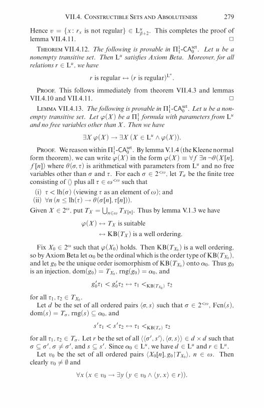
i

i

i

i

i

i

i

i


Hence v = x : rx is not regular ∈ Luâ+2. This completes the proof oflemma VII.4.11. 2

Theorem VII.4.12. The following is provable in Π11-CAset0 . Let u be a

nonempty transitive set. Then Lu satisfies Axiom Beta. Moreover, for allrelations r ∈ Lu , we have

r is regular↔ (r is regular)Lu .Proof. This follows immediately from theorem VII.4.3 and lemmasVII.4.10 and VII.4.11. 2

Lemma VII.4.13. The following is provable in Π11-CAset0 . Let u be a non-

empty transitive set. Let ϕ(X ) be a Π11 formula with parameters from Lu

and no free variables other than X . Then we have

∃X ϕ(X )→ ∃X (X ∈ Lu ∧ ϕ(X )).Proof. WereasonwithinΠ11-CA

set0 . By lemmaV.1.4 (theKleenenormal

form theorem), we can write ϕ(X ) in the form ϕ(X ) ≡ ∀f ∃n ¬è(X [n],f[n]) where è(ó, ô) is arithmetical with parameters from Lu and no freevariables other than ó and ô. For each ó ∈ 2<ù, let Tó be the finite treeconsisting of 〈〉 plus all ô ∈ ù<ù such that(i) ô < lh(ó) (viewing ô as an element of ù); and(ii) ∀n (n ≤ lh(ô)→ è(ó[n], ô[n])).Given X ∈ 2ù , put TX =

⋃n∈ù TX [n]. Thus by lemma V.1.3 we have

ϕ(X )↔ TX is suitable↔ KB(TX ) is a well ordering.

Fix X0 ∈ 2ù such that ϕ(X0) holds. Then KB(TX0) is a well ordering,so byAxiomBeta let α0 be the ordinal which is the order type of KB(TX0),and let g0 be the unique order isomorphism of KB(TX0) onto α0. Thus g0is an injection, dom(g0) = TX0 , rng(g0) = α0, and

g ′0ô1 < g′0ô2 ↔ ô1 <KB(TX0 ) ô2

for all ô1, ô2 ∈ TX0 .Let d be the set of all ordered pairs 〈ó, s〉 such that ó ∈ 2<ù, Fcn(s),dom(s) = Tó , rng(s) ⊆ α0, and

s ′ô1 < s′ô2 ↔ ô1 <KB(Tó) ô2

for all ô1, ô2 ∈ Tó . Let r be the set of all 〈〈ó ′, s ′〉, 〈ó, s〉〉 ∈ d ×d such tható ⊆ ó ′, ó 6= ó ′, and s ⊆ s ′. Since α0 ∈ Lu , we have d ∈ Lu and r ∈ Lu .Let v0 be the set of all ordered pairs 〈X0[n], g0TX0〉, n ∈ ù. Thenclearly v0 6= ∅ and

∀x (x ∈ v0 → ∃y (y ∈ v0 ∧ 〈y, x〉 ∈ r)).

i

i

i

i

i

i

i

i

280 VII. â-Models

Hence r is not regular. Hence by lemma VII.4.11 there exists v ∈ Lu suchthat v 6= ∅ and

∀x (x ∈ v → ∃y (〈y, x〉 ∈ r ∧ y ∈ v)).Since d = field(r) is well ordered in Lu , we can find a sequence 〈〈ón, sn〉:n < ù〉 ∈ Lu such that 〈ón, sn〉 ∈ v and 〈〈ón+1, sn+1〉, 〈ón , sn〉〉 ∈ r for alln < ù. Putting X =

⋃n∈ù ón and g =

⋃n∈ù sn, we see that X ∈ 2ù ,

dom(g) = TX , rng(g) ⊆ α0, andg ′ô1 < g

′ô2 ↔ ô1 <KB(TX ) ô2for all ô1, ô2 ∈ TX . Hence TX is suitable, i.e., ϕ(X ) holds. Also X ∈ Luby construction. This completes the proof of lemma VII.4.13. 2

The next theorem is our formalized version of the Shoenfield absolute-ness theorem within Π11-CA

set0 . It will be applied in the next section to

prove conservation results.

Theorem VII.4.14 (Shoenfield absoluteness in Π11-CAset0 ). The following

is provable inΠ11-CAset0 . Let u be a nonempty transitive set. Let ϕ be any Σ

12

sentence with parameters from Lu . Then ϕ ↔ ϕLu , i.e., ϕ is absolute to Lu .Proof. This is an immediate consequence of lemma VII.4.13. 2

Corollary VII.4.15. The following is provable in Π11-CAset0 . Let u be a

nonempty transitive set. The transitive model Lu satisfies V = Lu plus allaxioms ofΠ11-CA

set0 except possibly the Axiom of Countability.

Proof. By corollary VII.4.9 and theorems VII.4.3 and VII.4.12, Lu

satisfiesV = Lu plusATRset0 except possibly for theAxiomof Countability.

It remains to show that Lu satisfies Π11-CA0. By theorem VII.1.12 itsuffices to prove that Lu is closed under hyperjump. Let X ∈ Lu , X ⊆ ùbe given. By Π11-CA0 we have ∃Y (Y = HJ(X )). This is Σ12 so by theShoenfield absoluteness theorem VII.4.14, there exists Y ∈ Lu such thatLu satisfies Y = HJ(X ). By another application of VII.4.14 it followsthat Y = HJ(X ). This completes the proof. 2

Exercise VII.4.16. Show that the following is provable inΠ11-TRset0 . Let

u be a nonempty transitive set. Then Lu satisfies V = Lu plus all axiomsof Π11-TR

set0 except possibly the Axiom of Countability.

Remarks VII.4.17. Roughly speaking, the content of corollaryVII.4.15is that Π11-CA0 proves its own relativization to the inner model L

u . Exer-cise VII.4.16 gives the same result for Π11-TR0. In §VII.5 below, we shallobtain a similar result for stronger systems ∆12-CA0, Π12-CA0, Π12-TR0,∆13-CA0, Π13-CA0, etc.The phrase “except possibly the Axiom of Countability” cannot bedropped from corollary VII.4.15 or exercise VII.4.16. Indeed, Fefer-man and Levy have exhibited a transitive model of Π1∞-CA

set0 (see def-

inition VII.4.33 below) in which, for all nonempty transitive sets u,

i

i

i

i

i

i

i

i


the Axiom of Countability fails in Lu . The transitive model exhibitedby Feferman and Levy is Mset where M is as in remark VII.6.3 be-low.In order to restore the Axiom of Countability, we shall now pass to asmaller inner model HCL(X ), where X ⊆ ù. See definition VII.4.22 andtheorem VII.4.27 below. Some of our results about HCL(X ) will also beof use in §VII.5.

Definition VII.4.18. Within ATRset0 we make the following definitions.

1. A linear ordering is a relation ≺ such that, writing y ≺ x for〈y, x〉 ∈≺, one has(i) ∀x ∀y ((x ∈ field(≺) ∧ y ∈ field(≺)) → (x ≺ y ∨ x = y ∨y ≺ x));

(ii) ∀x ∀y ∀z ((z ≺ y ∧ y ≺ x)→ z ≺ x); and(iii) ¬∃x (x ≺ x).

2. If ≺ and ≺1 are linear orderings, we say that≺ is an initial segmentof ≺1 if ≺= ≺1field(≺). By definition VII.3.2.14 this implies

∀x ∀y ((y ≺1 x ∧ x ∈ field(≺))→ y ∈ field(≺)).

3. A linear ordering of u is a linear ordering ≺ such that field(≺) = u.4. A well ordering of u is a linear ordering of u which is regular.

Lemma VII.4.19. Within ATRset0 , let u be a nonempty transitive set.

1. Given a well ordering≺ of u, we can canonically define a well ordering≺∗ of def(u). Moreover ≺ is an initial segment of ≺∗.

2. Given a well ordering <0 of u, we can associate to each ordinal α acanonically defined well ordering <α of Luα . Moreover, for all â < α,<â is an initial segment of<α .

3. The definitions of ≺∗ and <α are absolute to Lu (provided ≺ and <0belong to Lu).

Proof. This is essentially Godel’s argument for the axiom of choice.To prove part 1, let Fu be the set of formulas of Lset with parametersfrom u and exactly one free variable. The given well ordering ≺ of ucanonically induces a well ordering ≺F of Fu . For all v ∈ def(u), let h′vbe the ≺F -least formula ϕ(x) ∈ Fu such that

v = x : x ∈ u ∧ 〈u,∈u〉 |= ϕ(x).

For v ∈ def(u) and w ∈ def(u), put w ≺∗ v if and only if either(i) w ∈ u ∧ v ∈ u ∧w ≺ v, or(ii) w ∈ u ∧ v ∈ def(u)− u, or(iii) w ∈ def(u)− u ∧ v ∈ def(u)− u ∧ h′w ≺F h′v.Clearly ≺∗ has the desired properties.

i

i

i

i

i

i

i

i

282 VII. â-Models

For part 2, <α is defined uniquely so that

∃f (Fcn(f) ∧ dom(f) = α + 1 ∧ f′α =<α

∧ f′0 =<0 ∧∀â (â < α → f′â + 1 = (f′â)∗)∧ ∀ä ((ä ≤ α ∧ Lim(ä))→ f′ä =

⋃f′′ä)).

Here ∗ is as in part 1. The proof of part 3 is straightforward. 2

Definition VII.4.20. The following definition is made within ATRset0 .

Given X ⊆ ù, note that ù ∪ X is a nonempty transitive set and putLα(X ) = L

ù∪Xα and L(X ) = Lù∪X. Let <L(X )0 be the well ordering of

ù ∪ X given by

<L(X )0 =

∈ù if X ∈ ù,(∈ù) ∪ (ù × X) otherwise.

Then for all ordinals α, let <L(X )α be the canonically associated well or-dering of Lα(X ) as in lemma VII.4.19. For u ∈ L(X ) and v ∈ L(X ), putv <L(X ) u if and only if ∃α (v <L(X )α u). We refer to<L(X ) as the canonicalwell ordering of L(X ).

Lemma VII.4.21. Provably in ATRset0 , the formulas u ∈ L(X ), v <L(X ) u

and w = v : v <L(X ) u are Σset1 and absolute to L(X ).Proof. This is similar to the proof of lemma VII.4.6.1 and theoremVII.4.8. 2

Definition VII.4.22 (the inner model HCL(X )). Within ATRset0 , as-

sume X ⊆ ù. We write u ∈ HCL(X ) to mean that u is hereditarilyconstructibly countable from X , i.e.,

∃f (f ∈ L(X ) ∧ Fcn(f) ∧ dom(f) = ù ∧ u ⊆ rng(f) ∧ Trans(rng(f))).If ϕ is any formula of Lset, the relativization of ϕ to HCL(X ) is writtenϕHCL(X ) and is defined in the obvious way, exactly as for ϕL(X ) (defini-tion VII.4.5). We sometimes express ϕHCL(X ) by saying that HCL(X )satisfies ϕ.

Obviously HCL(X ) is a transitive submodel of L(X ), i.e.,∀u (u ∈ HCL(X ) → u ∈ L(X )) and ∀u ∀v ((v ∈ u ∧ u ∈ HCL(X )) →v ∈ HCL(X )). In addition we have ∀u ∀v ((u ∈ HCL(X ) ∧ v ⊆ u ∧v ∈ L(X ))→ v ∈ HCL(X )).Lemma VII.4.23. Provably in ATR

set0 we have:

1. The formula u ∈ HCL(X ) is equivalent to a Σset1 formula.2. If ϕ is any Σsetk formula, 0 ≤ k < ù, then ϕHCL(X ) is equivalent to aΣsetk formula.

Proof. This is exactly like the proof of lemma VII.4.6. 2

i

i

i

i

i

i

i

i


Definition VII.4.24. We say that ϕ is absolute to HCL(X ) if

∀x1 · · · ∀xm ((x1 ∈ HCL(X ) ∧ · · · ∧ xm ∈ HCL(X ))→ (ϕ ↔ ϕHCL(X )))holds, where x1, . . . , xm are the free variables of ϕ.

We sometimes write V = HCL(X ) as an abbreviation for ∀u (u ∈HCL(X )).

Lemma VII.4.25. WithinATRset0 , assumeX ⊆ ù. Ifϕ is anyΣset1 sentence

with parameters fromHCL(X ), we have

ϕL(X ) ↔ ϕHCL(X ).Proof. Since HCL(X ) ⊆trans L(X ), it is clear ϕHCL(X ) implies ϕL(X ).We shall prove the converse. This will be essentially Godel’s argument forthe continuum hypothesis.Assume ϕL(X ). The parameters of ϕ belong to HCL(X ), so let u ∈HCL(X ) be transitive and contain these parameters. Write ϕ as ∃x è(x)where è(x) is ∆set0 with the same parameters as ϕ. Fix z ∈ L(X ) such thatè(z) holds in L(X ). Let ä be a limit ordinal such that u ⊆ Lä(X ) andz ∈ Lä(X ). Hence è(z) holds in Lä(X ).Let v be the smallest subset of Lä(X ) such that u ⊆ v, z ∈ v, and v isclosed under definability in the language =, ∈, < over the model

〈Lä(X ),∈Lä(X ), <L(X )ä 〉.

Since <L(X )ä is a well ordering of Lä(X ), v is an elementary submodel of

〈Lä(X ),∈Lä(X )〉. In particular v satisfies è(z). Also, since<L(X )ä ∈ L(X )and u is countable in L(X ), it follows that v is countable in L(X ), i.e.,there exists a function g ∈ L(X ) such that dom(g) = ù and rng(g) = v.Let f be the collapsing function of v, i.e., f is the unique function suchthat dom(f) = v and

f′x = f′′y : y ∈ v ∧ y ∈ xfor all x ∈ v. Put w = rng(f). Thus w is transitive and f is the unique∈-isomorphism of v onto w. By lemma VII.4.10 we have f ∈ L(X ),hence fg ∈ L(X ). Since dom(fg) = ù and rng(fg) = w, it follows thatw ∈ HCL(X ).The transitivity of u implies that y = f′y ∈ w for all y ∈ u. In par-ticular this holds for all of the parameters y of è(x). Therefore 〈w,∈w〉satisfies è(f′z). Since w ⊆trans HCL(X ), we see that HCL(X ) satisfiesè(f′z). Thus HCL(X ) satisfies ∃x è(x), i.e., ϕ.This completes the proof of lemma VII.4.25. 2

Lemma VII.4.26. The following is provable in ATRset0 . For X ⊆ ù, the

formulas u ∈ HCL(X ), u = Lα(X ), v <L(X ) u, and w = v : v <L(X ) uare Σset1 and absolute to HCL(X ). In particular, HCL(X ) satisfies V =HCL(X ).

i

i

i

i

i

i

i

i

284 VII. â-Models

Proof. By theorem VII.4.8 and lemmas VII.4.6.1, VII.4.21, andVII.4.23.1, the mentioned formulas are Σset1 and absolute to L(X ). Henceby lemma VII.4.25 they are absolute to HCL(X ). 2

Theorem VII.4.27. The following is provable in Π11-CAset0 . Assume X ⊆

ù. Then:

1. HCL(X ) satisfies V = HCL(X ) plus all axioms ofΠ11-CAset0 .

2. All Σ12 and Σset1 formulas are absolute to HCL(X ). In other words,

ϕ ↔ ϕHCL(X ) holds for all Σ12 or Σset1 sentences ϕ with parameters

fromHCL(X ).

Proof. Part 1 follows from corollary VII.4.15 and lemma VII.4.26.Part 2 follows frompart 1, theoremVII.4.14 (absoluteness of Σ12 formulas)and theorem VII.3.24 (equivalence of Σ12 with Σ

set1 ). 2

Exercise VII.4.28.WithinATRset0 , assumingX ⊆ ù, show thatHCL(X )

satisfies V = HCL(X ) plus all axioms of ATRset0 except possibly Axiom

Beta.

Exercise VII.4.29. Exhibit a transitivemodelofATRset0 inwhichHCL(∅)

does not satisfy Axiom Beta. Show that ATRset0 proves the following: Π

11-

CA0 if and only if

∀X (X ⊆ ù → (Axiom Beta)HCL(X )).Exercise VII.4.30. Exhibit a transitive model of ATR

set0 in which not

all Σ11 sentences are absolute to HCL(∅). Show that ATRset0 proves the

following: Π11-CA0 if and only if all Σ11 formulas are absolute to HCL(X )for all X ⊆ ù.Exercise VII.4.31. Within ATR

set0 , assuming X ⊆ ù, show that if the

hyperjump Y = HJ(X ) exists then Y ∈ HCL(X ) and HCL(X ) satisfiesY = HJ(X ).

Exercise VII.4.32. Let ϕ(X,Y ) be a Π11 formula with no free variablesother than X and Y . Prove in ATR

set0 that for all X ⊆ ù, if there

exists Y such that ϕ(X,Y ) holds and HJ(X ⊕Y ) exists, then there existsY ∈ HCL(X ) such that ϕ(X,Y ) holds. (This is a refinement of lemmaVII.4.13.)

We end this section with a theorem concerning the special situationwhen HCL(X ) is not all of L(X ). The conclusion in this case is ratherstrong.

Definition VII.4.33. Π1∞-CAset0 is the theory in Lset which consists of

ATRset0 plus the full comprehension scheme:

∀u ∃v ∀x (x ∈ v ↔ (x ∈ u ∧ ϕ(x)))where ϕ(x) is any formula of Lset in which v does not occur freely. (Seealso lemma VII.5.3.)

i

i

i

i

i

i

i

i


Theorem VII.4.34. The following is provable in ATRset0 . AssumeX ⊆ ù.

Suppose thatHCL(X ) 6= L(X ). Then:1. HCL(X ) = Lä(X ) for a certain limit ordinal ä.2. HCL(X ) satisfies V = HCL(X ) plus all axioms ofΠ1∞-CA

set0 .

3. HCL(X ) satisfies Axiom Beta. Moreover, for all relations r ∈HCL(X ), we have

r is regular↔ (r is regular)HCL(X ).4. HCL(X ) is closed under hyperjump. All Σ11 formulas are absolute toHCL(X ).

Proof. By lemmas VII.4.25 and VII.4.26, we have u ∈ HCL(X ) if andonly if ∃α (u ∈ Lα(X ) ∧ Lα(X ) ∈ HCL(X )). If HCL(X ) 6= L(X ), itfollows that there exists an ordinal ã such that Lã(X ) /∈ HCL(X ). HenceHCL(X ) ⊆ Lã(X ). Let ä be the set of all α < ã such that

∃f (f ∈ Lã(X ) ∧ Fcn(f) ∧ dom(f) = ù ∧ rng(f) = Lα(X )).Then clearly ä is a limit ordinal and Lä(X ) = HCL(X ). This provespart 1. (It can be shown that ä is the smallest uncountable ordinal ofL(X ).)For part 2, let ϕ(x) be a formula of Lset with parameters fromHCL(X )and no free variables other than x. Given u ∈ HCL(X ) = Lä(X ), put

v = x : x ∈ u ∧ 〈Lä(X ),∈Lä(X )〉 |= ϕ(x).Thus v ∈ Lä+1(X ). Since v ⊆ u and u ∈ HCL(X ), it follows triviallythat v ∈ HCL(X ). Then clearly HCL(X ) = Lä(X ) satisfies ∀x (x ∈v ↔ (x ∈ u ∧ ϕ(x))). This shows that HCL(X ) is a model of fullcomprehension.By lemma VII.4.26, HCL(X ) satisfies V = HCL(X ). By theoremVII.4.3.7, HCL(X ) = Lä(X ) satisfies Bset0 . It is obvious that HCL(X )satisfies the Axioms of Regularity and Countability. It remains to provethat HCL(X ) satisfies Axiom Beta.Let r ∈ HCL(X ) be a relation. If r is regular, lemma VII.4.10 impliesthat the collapsing function of r belongs to HCL(X ). Suppose now thatr is not regular. We shall use the notation rx which was introduced inthe proof of lemma VII.4.11. Let w be the set of x ∈ field(r) such thatthe collapsing function of rx is an element of HCL(X ). Since HCL(X )is a transitive model of full comprehension, w ∈ HCL(X ). Put v =field(r) − w. Then v ∈ HCL(X ) and, since r is not regular, v 6= ∅. Ifx ∈ field(r) and ∀y (〈y, x〉 ∈ r → y ∈ w), then rx is regular, hence bylemma VII.4.10 x ∈ w. Hence ∀x (x ∈ v → ∃y (〈y, x〉 ∈ r ∧ y ∈ v)).Thus (r is not regular)HCL(X ).Combining these observations, we see that HCL(X ) satisfies AxiomBeta. This completes the proof of part 2 and also proves part 3.

i

i

i

i

i

i

i

i

286 VII. â-Models

To prove part 4, let ϕ be a Σ11 sentence with parameters from HCL(X ).By theKleenenormal formtheoremV.1.4, we canwriteϕ as∃f ∀n è(f[n])where è(ô) is arithmetical with parameters from HCL(X ). Let r be theset of all 〈ôa〈k〉, ô〉 such that ∀n (n ≤ lh(ô) → è(ô[n])). Using part 3 wesee that

ϕ ↔ r is not regular↔ (r is not regular)HCL(X )

↔ ϕHCL(X ).This shows that all Σ11 formulas are absolute to HCL(X ). In other words,HCL(X ) is a â-model. Also, frompart 2 it follows a fortiori thatHCL(X )satisfies Π11-CA0. Hence by theorem VII.1.12 HCL(X ) is closed underhyperjump.This completes the proof of theorem VII.4.34. 2

Exercise VII.4.35. Exhibit a transitive model of ATRset0 in which

HCL(∅) 6= L(∅), yet not all Σ12 or Σset1 sentences are absolute to HCL(∅).

Notes for §VII.4. Godel’s original papers [95, 96] on constructible setsare still worth reading. Godel’s subsequent detailed treatment [97] ismuch less accessible. For further information on constructible sets, seeJensen [131] or any good textbook of axiomatic set theory, e.g., Jech[130]. The original Shoenfield absoluteness theorem is due to Shoenfield[221] and is closely related to Kondo’s theorem (§VI.2). Our observationthat the Shoenfield absoluteness theorem is provable in Π11-CA0 (theoremVII.4.14) was inspired by Jensen/Karp [132] and Barwise/Fisher [14] (seealso Barwise [13, §V.8]). Our theorem VII.4.27.2 on Σset1 absoluteness issimilar to a result of Levy [162, theorem 43].

VII.5. Strong Comprehension Schemes

In this and the next two sections, we study â-models of certain subsys-tems of second order arithmetic which are stronger than Π11-CA0. We relyon the set-theoretic results of the previous two sections.

Definition VII.5.1 (comprehension schemes). Assume 0 < k < ù.

1. Π1k-CA0 is the subsystem of Z2 which consists of ACA0 plus thescheme of Π1k comprehension:

∃X ∀n (n ∈ X ↔ ø(n))where ø(n) is any Π1k formula in which X does not occur freely.

2. ∆1k-CA0 is the subsystemofZ2which consists ofACA0 plus the schemeof ∆1k comprehension:

∀n (ϕ(n)↔ ø(n))→ ∃X ∀n (n ∈ X ↔ ø(n))

i

i

i

i

i

i

i

i

VII.5. Strong Comprehension Schemes 287

where ϕ(n) is any Σ1k formula and ø(n) is any Π1k formula in which

X does not occur freely.3. Π1∞-CA0 =

⋃k<ù Π

1k-CA0.

Remarks VII.5.2. Obviously

∆1k-CA0 ⊆ Π1k-CA0 ⊆ ∆1k+1-CA0

for all k, 0 ≤ k < ù. We shall see later that all of these inclusionsare proper except for the triviality ACA0 = ∆10-CA0 = Π10-CA0. Thedevelopment of mathematics within ACA0 has been discussed in chapterIII. By theorem V.5.1 we have

∆11-CA0 ⊆ ATR0 ⊆ Π11-CA0.

Further results on models of ACA0 and ∆11-CA0 will be presented in chap-ters VIII and IX. The development of mathematics within Π11-CA0 hasbeen discussed in chapter VI. Models of Π11-CA0 have been discussedin §§VII.1 and VII.4 in the present chapter. Models of Π1k+1-CA0 and

∆1k+2-CA0 are the principal topic of this and the next two sections. Fur-

ther results on models of Π1k+1-CA0 and ∆1k+2-CA0 will be presented inchapters VIII and IX.In order to prove theorems about models of Π1k+1-CA0 and ∆1k+2-CA0,it will be convenient to work with the set-theoretic counterparts of thesetheories. Recall that to each L2-theory T0 ⊇ ATR0, we have associateda set-theoretic counterpart T set0 consisting of ATR

set0 plus T0. Thus T

set0

is a theory in the language Lset and proves the same L2-sentences as T0(theorem VII.3.34). The purpose of the following lemma is to identifyeach of Π1k+2-CA

set0 and ∆

1k+2-CA

set0 .

Lemma VII.5.3. Assume 0 ≤ k < ù. Over ATRset0 we have:

1. Π1k+2-CA0 is equivalent to the scheme ofΠsetk+1 comprehension:

∀u ∃v ∀x (x ∈ v ↔ (x ∈ u ∧ ø(x)))where ø(x) is anyΠsetk+1 formula in which v does not occur freely.

2. ∆1k+2-CA0 is equivalent to the scheme of ∆setk+1 comprehension:

∀x (ϕ(x)↔ ø(x))→ ∀u ∃v ∀x (x ∈ v ↔ (x ∈ u ∧ ø(x)))where ϕ(x) is any Σsetk+1 formula and ø(x) is any Π

setk+1 formula in

which v does not occur freely.

Proof. This follows easily from the intertranslatability of Σ1k+2 withΣsetk+1 (theorem VII.3.24) together with the equivalence of ATR0 with

|ATRset0 | (theorem VII.3.22). 2

We shall now show that each of Π1k+1-CA0 and ∆1k+2-CA0, 0 ≤ k < ùimplies its own relativization to the inner model HCL(X ) (definitionVII.4.22).

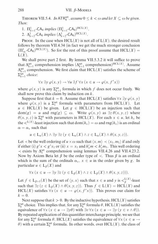
i

i

i

i

i

i

i

i

288 VII. â-Models

Theorem VII.5.4. InATRset0 , assume 0 ≤ k < ù and letX ⊆ ù be given.

Then:

1. Π1k+1-CA0 implies (Π1k+1-CA0)HCL(X ).

2. ∆1k+2-CA0 implies (∆1k+2-CA0)HCL(X ).

Proof. In the case when HCL(X ) is not all of L(X ), the desired resultfollows by theorem VII.4.34 (in fact we get the much stronger conclusion(Π1∞-CA0)HCL(X )). So for the rest of this proof assume that HCL(X ) =L(X ).We shall prove part 2 first. By lemma VII.5.3.2 it will suffice to provethat ∆setk+1 comprehension implies (∆

setk+1 comprehension)

HCL(X ). Assume∆setk+1 comprehension. We first claim that HCL(X ) satisfies the scheme ofΣsetk+1 choice:

∀x ∃y ϕ(x, y)→ ∀u ∃f ∀x (x ∈ u → ϕ(x,f′x))

where ϕ(x, y) is any Σsetk+1 formula in which f does not occur freely. Weshall now prove this claim by induction on k.Suppose first that k = 0. Assume that HCL(X ) satisfies ∀x ∃y ϕ(x, y)where ϕ(x, y) is a Σset1 formula with parameters from HCL(X ). Letu ∈ HCL(X ) be given. Let g ∈ HCL(X ) be an injection such thatdom(g) = u and rng(g) ⊆ ù. Write ϕ(x, y) as ∃z è(x, y, z) whereè(x, y, z) is Σset0 with parameters in HCL(X ). For each x ∈ u, let hx bethe<L(X )-least injection such that dom(hx) = ù and rng(hx) is an ordinalα = αx such that

u ∈ Lα(X ) ∧ ∃y ∃z (y ∈ Lα(X ) ∧ z ∈ Lα(X ) ∧ è(x, y, z)).Let≺ be the well ordering of u×ù such that 〈x,m〉 ≺ 〈x1, m1〉 if and onlyif either (i) g ′x < g ′x1 or (ii) x = x1 and h′xm < h

′xm1. This well ordering

≺ exists by ∆set1 comprehension using lemmas VII.4.26 and VII.4.23.2.Now by Axiom Beta let â be the order type of ≺. Thus â is an ordinalwhich is the sum of the ordinals αx , x ∈ u in the order given by g. Inparticular u ∈ Lâ(X ) and

∀x (x ∈ u → ∃y ∃z (y ∈ Lâ(X ) ∧ z ∈ Lâ(X ) ∧ è(x, y, z))).

Let f ∈ Lâ+1(X ) be the set of 〈y, x〉 such that x ∈ u and y is <L(X )â -least

such that ∃z (z ∈ Lâ(X ) ∧ è(x, y, z)). Thus f ∈ L(X ) = HCL(X ) andHCL(X ) satisfies ∀x (x ∈ u → ϕ(x,f′x)). This proves our claim fork = 0.Next suppose thatk > 0. By the inductive hypothesis, HCL(X ) satisfiesΣsetk choice. This implies that, for any Σ

setk formula è, HCL(X ) satisfies the

equivalence of ∀x (x ∈ u → ∃yè) with ∃v ∀x (x ∈ u → ∃y (y ∈ v ∧ è)).By repeated application of this quantifier interchangeprinciple, we see thatfor any Σsetk formula è, HCL(X ) satisfies the equivalence of ∀x (x ∈ u →è) with a certain Σsetk formula. In other words, over HCL(X ), the class of

i

i

i

i

i

i

i

i


Σsetk formulas is closed under bounded quantification. Keep in mind also

that by lemma VII.4.23, for any Σsetk formula è, the relativization èHCL(X )

is also Σsetk .Assume now thatHCL(X ) satisfies ∀x ∃y ϕ(x, y) where ϕ(x, y) is Σsetk+1with parameters in HCL(X ). Let u ∈ HCL(X ) be given. Let g be asbefore. Write ϕ(x, y) as ∃z è(x, y, z) where è(x, y, z) is Πsetk . For eachx ∈ u, let hx be the <L(X )-least injection such that dom(hx) = ù andrng(hx) is an ordinal α = αx such that HCL(X ) satisfies ∃y ∃z (y ∈Lα(X ) ∧ z ∈ Lα(X ) ∧ è(x, y, z)). Define ≺ as before. This well ordering≺ exists by ∆setk+1 comprehension using lemma VII.4.26 and the aboveobservations concerning bounded quantifiers. Define â as before. Let

f be the set of all 〈y, x〉 such that x ∈ u and y is <L(X )â -least such that

HCL(X ) satisfies ∃z (z ∈ Lâ(X ) ∧ è(x, y, z)). By our observations onbounded quantifiers, this definition of f is ∆setk . By induction on k,HCL(X ) satisfies ∆setk comprehension. Hence f ∈ HCL(X ), and clearlyHCL(X ) satisfies ∀x (x ∈ u → ϕ(x,f′x)). This proves our claim.To complete the proof of part 2, assume that HCL(X ) satisfies ∀x(ϕ(x)↔ ø(x)) where ϕ(x) and ø(x) are Σsetk+1, respectively Πsetk+1 formu-las with parameters in HCL(X ). Let ç(x, y) be the Σsetk+1 formula

(y = 1 ∧ ϕ(x)) ∨ (y = 0 ∧ ¬ø(x)).Then HCL(X ) satisfies ∀x ∃y ç(x, y). Given u ∈ HCL(X ), apply Σsetk+1choice in HCL(X ) to obtain f ∈ HCL(X ) such that HCL(X ) satisfies∀x (x ∈ u → ç(x,f′x)). Putting v = x : x ∈ u ∧ f′x = 1, we seethat v ∈ HCL(X ) and HCL(X ) satisfies ∀x (x ∈ v ↔ (x ∈ u ∧ ø(x)).Thus HCL(X ) satisfies ∆setk+1 comprehension. This completes the proof ofpart 2.We shall now prove part 1. By lemma VII.5.3.1 it will suffice to provethat Πsetk+1 comprehension implies (Π

setk+1 comprehension)

HCL(X ). AssumeΠsetk+1 comprehension. Let ø(x) be a Π

setk+1 formula with parameters in

HCL(X ) and no free variables other than x. Let u ∈ HCL(X ) be given.By lemma VII.4.23 and Πsetk+1 comprehension, let v be the set of x ∈ usuch that HCL(X ) satisfies ø(x). Write ø(x) as ∀y è(x, y) where è(x, y)is Σsetk . As before, let â be a sum of ordinals αx , x ∈ u − v, whereα = αx is chosen so that ∃y (y ∈ Lα(X ) ∧ ¬è(x, y)). Thus v may bedescribed as the set ofx ∈ u such thatHCL(X ) satisfies∀y (y ∈ Lâ (X )→è(x, y)). By our observations concerning bounded quantifiers, the latterformula is equivalent over HCL(X ) to a Σsetk formula with parameters inHCL(X ). Applying Σsetk comprehension within HCL(X ), it follows thatv ∈ HCL(X ).This completes the proof of theorem VII.5.4. 2

Exercise VII.5.5. In ATRset0 , show that for all X ⊆ ù, L(X ) and

HCL(X ) satisfy Σset1 choice.

i

i

i

i

i

i

i

i

290 VII. â-Models

Exercise VII.5.6. Show that ∆set1 comprehension is equivalent overATR

set0 to Σ

set1 choice.

Exercise VII.5.7. Show that ∆set1 comprehension fails in the minimumtransitive model of Π11-CA

set0 . (By lemma VII.5.3 we may restate this as

follows: ∆12-CA0 fails in the minimum â-model of Π11-CA0.)

We shall now reformulate the previous theorem so as to apply directlyto subsystems of Z2 andmodels of same. Some of our results will be statedas conservation theorems (see definition VII.5.12 below).

Definition VII.5.8. In the language L2, we write Y ∈ L(X ) andZ <L(X ) Y as abbreviations for

∃V0 ∃V1 (V0 = X∗ ∧ V1 = Y∗ ∧ |v1 ∈ L(v0)|)and

∃V0 ∃V1 ∃V2 (V0 = X∗ ∧V1 = Y∗ ∧ V2 = Z∗ ∧ |v2 <L(v0) v1|)respectively. By lemma VII.4.21 and theorem VII.3.24.1, the above for-mulas are Σ12, provably in ATR0.

Remark VII.5.9. The point of the above definition is as follows. LetM be a model of ATR0. Given X,Y ∈ SM , identify X and Y with thecorresponding elements [X∗] and [Y∗] of |Mset| (definitions VII.3.18 andVII.3.28). Then M |= Y ∈ L(X ) if and only if Mset |= Y ∈ L(X ). Asimilar remark applies to the formula Z <L(X ) Y .

Theorem VII.5.10. Let M ′ be any model of Π11-CA0. Given X ∈ SM ′ ,let M be the ù-submodel of M ′ consisting of all Y ∈ SM ′ such thatM ′ |= Y ∈ L(X ). Then:1. M is a model ofΠ11-CA0.2. X ∈ SM , andM satisfies ∀Y (Y ∈ L(X )).3. M is a â2-submodel of M ′. This means that for any Σ12 sentence ϕwith parameters fromM ,M |= ϕ if and only ifM ′ |= ϕ.

4. IfM ′ is a â-model, then so isM .5. IfM ′ is an ù-model, then so isM .

Furthermore, for all k ≥ 0, we have:6. To any Σ1k+2 formula ϕ(n1, . . . , ni , X1, . . . , Xj) with parameters from

M , we can associate a Σ1k+2 formula ϕ′ such that, for all n1, . . . , ni ∈

|M | and X1, . . . , Xj ∈ SM ,M |= ϕ(n1, . . . , ni , X1, . . . , Xj)

if and only if

M ′ |= ϕ′(n1, . . . , ni , X1, . . . , Xj).

7. IfM ′ is model of ∆1k+2-CA0, then so isM .

i

i

i

i

i

i

i

i


8. IfM ′ is a model ofΠ1k+2-CA0, then so isM .

9. IfM ′ is a model ofΠ1∞-CA0, then so isM .

Proof. Clearly Mset is the transitive submodel of M ′set consisting of

all a ∈ |M ′set| such that M ′

set |= a ∈ HCL(X ). It follows by theoremVII.4.27.1 thatMset satisfies V = HCL(X ) plus all axioms of Π11-CA

set0 .

HenceM satisfies∀Y (Y ∈ L(X )) plusΠ11-CA0. This gives parts 1 and 2 ofthe theorem. Part 3 follows from theoremVII.4.14. Part 4 follows immedi-ately from part 3. Part 5 is trivial. For part 6, let ϕ(n1, . . . , ni , X1, . . . , Xj)be a given Σ1k+2 formula. By theorem VII.3.24.2, we may regard ϕ as a

Σsetk+1 formula of Lset. Hence by lemma VII.4.23.2, ϕHCL(X ) is Σsetk+1. Let

ϕ′(n1, . . . , ni , X1, . . . , Xj) be the L2-formula

∃V1 · · · ∃Vi ∃Vi+1 · · · ∃Vi+j(V1 = n

∗1 ∧ · · · ∧ Vi = n∗i ∧Vi+1 = X∗

1 ∧ · · · ∧ Vi+j = X∗j

∧ |ϕHCL(X )(v1, . . . , vi , vi+1, . . . , vi+j)|).

By theorem VII.3.24.1, ϕ′ is Σ1k+2, and clearly ϕ′ satisfies the conclusion

of part 6. Parts 7 and 8 follow from theorems VII.5.4.2 and VII.5.4.1respectively. Part 9 is an immediate consequence of part 8. 2

From the above theorem we can deduce the following key result.

Corollary VII.5.11 (conservation theorems). Let T0 be any one of theL2-theories Π1∞-CA0, Π1k+1-CA0, or ∆1k+2-CA0, 0 ≤ k < ù. Let ø be anyΠ14 sentence. Suppose that ø is provable from T0 plus ∃X ∀Y (Y ∈ L(X )).Then ø is provable from T0 alone.

Proof. Let ø be a Π14 sentence which is not provable from T0. ByGodel’s completeness theorem, let M ′ be a model of T0 plus ¬ø. Write¬ø as ∃X ∀Y ϕ(X,Y ) where ϕ(X,Y ) is a Σ12 formula. Let X ∈ SM ′

be such that M ′ |= ∀Y ϕ(X,Y ). Let M ⊆ù M ′ consist of all Y ∈SM ′ such that M ′ |= Y ∈ L(X ). By theorem VII.5.10, M satisfies T0plus ∀Y (Y ∈ L(X )) plus ∀Y ϕ(X,Y ). Thus M is a model of T0 plus∃X ∀Y (Y ∈ L(X )) plus ¬ø. Therefore, by the soundness theorem,ø is not provable from T0 plus ∃X ∀Y (Y ∈ L(X )). This proves thecorollary. 2

The content of the above corollary is that, when trying to prove aΠ14 sentence within T0, it is harmless to assume ∃X ∀Y (Y ∈ L(X )). Inother words, using the terminology of the following definition, T0 plus∃X ∀Y (Y ∈ L(X )) is conservative over T0 for Π14 sentences. Results ofthis kind are sometimes known as conservation theorems. Other conser-vation theorems will be presented in the next section and in chapter IX.

Definition VII.5.12 (conservativity). Let T0 and T′0 be theories in the

language L2. We say that T ′0 is conservative over T0 for Π

1k sentences if

i

i

i

i

i

i

i

i

292 VII. â-Models

T ′0 ⊇ T0 and any Π1k sentence which is provable in T ′

0 is already provablein T0.

Exercise VII.5.13 (more conservation theorems). Assume 0 ≤ k ≤m ≤ n ≤ ∞. Let T0 consist of either Π1k+1-CA0 or ∆1k+2-CA0, plus

Π1m+1-TI0 plus Σ1n+1-IND (definitions VII.5.1, VII.2.14, and VII.6.1.2).

Show that T0 plus ∃X ∀Y (Y ∈ L(X )) is conservative over T0 for Π14sentences.

Exercise VII.5.14 (ù-model conservation theorems). Assume0 ≤ k ≤m ≤ ∞. Let T0 consist of either Π1k+1-CA0 or ∆1k+2-CA0, plus Π1m+1-TI0.

Let ø be any Π14 sentence. Suppose that ø holds in all ù-models of T0plus ∃X ∀Y (Y ∈ L(X )). Show that ø holds in all ù-models of T0.Exercise VII.5.15 (â-model conservation theorems). Let T0 and ø beas in corollary VII.5.11. Suppose that ø holds in all transitive models ofT0 of the form Lα(X ), X ⊆ ù, α a countable ordinal. Show that ø holdsin all â-models of T0.

Exercise VII.5.16. Show that the results of corollary VII.5.11 and ex-ercises VII.5.13, VII.5.14 and VII.5.15 do not extend to Σ14 sentences.Hint: The sentence ∃X ∀Y (Y ∈ L(X )) is Σ14. Consider a transitivemodel of ZFC in which the continuum hypothesis does not hold.

We shall now apply theorem VII.5.10 to obtain the minimum â-modelsof Π1k+1-CA0 and ∆1k+2-CA0, 0 ≤ k < ù, and of Π1∞-CA0.

Theorem VII.5.17 (minimum â-models). Assume X ⊆ ù and 0 ≤k < ù.

1. Among all â-models of Π1k+1-CA0 which contain X , there is a unique

smallest oneM = MΠk+1(X ). FurthermoreMset can be characterized(up to canonical isomorphism) as Lα(X ) for a certain ordinal α =αΠk+1(X ), namely the smallest ordinal α such that Lα(X ) satisfies

Π1k+1 comprehension.

2. Same as part 1 with Π1k+1, MΠk+1(X ), α

Πk+1(X ) replaced by ∆

1k+2,

M∆k+2(X ), α∆k+2(X ) respectively.

3. Same as part 1 with Π1k+1, MΠk+1(X ), α

Πk+1(X ) replaced by Π

1∞,

MΠ∞(X ), αΠ∞(X ) respectively.

Proof. Let M ′ be any â-model of Π1k+1-CA0 which contains X . LetM ⊆ù M ′ consist of all Y ∈ M ′ such that M ′ |= Y ∈ L(X ). Bytheorem VII.5.10,M is a â-model of Π1k+1-CA0 andM satisfies ∀Y (Y ∈L(X )). Thus Mset is isomorphic to a transitive model of Π1k+1-CA

set0

plus V = HCL(X ). By lemma VII.4.21, this model is Lâ (X ) for someordinal â . Then clearly â ≥ α where α = αΠk+1(X ) is as defined in thestatement of part 1. Put MΠk+1(X ) = (Lα(X ))

2. Then MΠk+1(X ) satisfies

Π1k+1-CA0 by definition, and is a â-model by theorem VII.3.27.2. Also

i

i

i

i

i

i

i

i


MΠk+1(X ) ⊆M ⊆M ′ so part 1 is proved. The proofs of parts 2 and 3 aresimilar. 2

Remark VII.5.18. In §VII.7 we shall see that for all X ⊆ ù and 0 ≤k < ù,

αΠk+1(X ) < α∆k+2(X ) < α

Πk+2(X ).

In §§VIII.3 and VIII.4 we shall obtain an analogous ordinal α∆1 (X ) <αΠ1 (X ). Namely, setting α = α

∆1 (X ) = sup|a|X : O(a,X ) and M =

M∆1 (X ) = HYP(X ), we shall see thatM = Lα(X )∩P(ù) is theminimumù-model of ∆11-CA0.

Exercise VII.5.19 (minimum â-submodels). Assume 0 ≤ k < ù andlet X ∈ M ′ |= Π1k+1-CA0 be given. Prove that among all â-submodels

M ⊆â M ′ such that X ∈ M |= Π1k+1-CA0, there is a unique smallest

one. Describe this model. Prove similar results with Π1k+1-CA0 replaced

by ∆1k+2-CA0 and by Π1∞-CA0.

Exercise VII.5.20. Recall the system Π1k-TR0, definition VI.7.1. Ex-tendVII.5.10–VII.5.19 to encompassΠ1k+1-TR0, 0 ≤ k < ù. In particularwe have a result similar to VII.5.17.1 with Π1k+1-CA0, MΠk+1(X ), α

Πk+1(X ),

Π1k+1 comprehension replaced by Π1k+1-TR0, MΠ

∗

k+1(X ), αΠ∗

k+1(X ), Π1k+1

transfinite recursion respectively. Thus we obtain minimum â-models ofΠ1k+1-TR0, 0 ≤ k < ù. (See also exercises VII.7.12.)

Notes for §VII.5. The ideas of this section are probably well known, butwe have been unable to find bibliographical references for them. Oursharp formulations VII.5.10–VII.5.16 in terms of conservation results areprobably new.Our results on minimum â-models of ∆1k-CA0 and Π1k-CA0 are closelyrelated to some well known ideas of Barwise and Jensen. In order toexplain this connection, let us use the notation of VII.5.17 and VII.5.18and write α∆k = α

∆k (∅) and αΠk = αΠk (∅), where ∅ is the empty set. For k =

1, the ordinals α∆1 and αΠ1 can be characterized in terms of admissibility

theory, as discussed in Barwise [13], Simpson [233], and Sacks [211].Namely, α∆1 = ù

CK1 = the least admissible ordinal > ù, and αΠ1 = the

supremum of the first ù admissible ordinals. (Note however that αΠ1 isnot itself admissible.) Moreover, for arbitrary k < ù, the ordinals α∆k+2and αΠk+2 can be characterized in terms of Jensen’s fine structure theory

[131]; see also Simpson [233, §3]. Namely, α∆k+2 = the least α such thatçαk+1 > ù, or equivalently the least α > ù such that ç

αk+1 = α; and

αΠk+2 = the least α such that ñαk+1 > ù, or equivalently the least α > ù

such that ñαk+1 = α. These results are easily deduced from theoremsVII.3.24 and VII.5.17.

i

i

i

i

i

i

i

i

294 VII. â-Models

VII.6. Strong Choice Schemes

The purpose of this section is to study the axiomof choice in the contextof second order arithmetic. We shall consider several choice schemes, i.e.,axiom schemes in the language L2 which express consequences or specialcases of the axiom of choice. We shall obtain some conservation theoremsrelating strong choice schemes to strong comprehension schemes. Wemake essential use of the results of the previous two sections.

Definition VII.6.1 (choice schemes). Assume 0 ≤ k < ù.1. Σ1k-AC0 is the L2-theory whose axioms are those of ACA0 plus thescheme of Σ1k choice:

∀n ∃Y ç(n,Y )→ ∃Z ∀n ç(n, (Z)n)where ç(n,Y ) is any Σ1k formula in which Z does not occur. We areusing the notation

(Z)n = i : (i, n) ∈ Z.2. Σ1k-IND is the scheme of Σ1k induction:

(ϕ(0) ∧ ∀n (ϕ(n)→ ϕ(n + 1)))→ ∀n ϕ(n)where ϕ(n) is any Σ1k formula. We also define Σ

1∞-IND =

⋃k<ù Σ

1k-

IND. Note that Σ1∞-IND automatically holds in all ù-models.3. Σ1k-DC0 is the L2-theory whose axioms are those of ACA0 plus thescheme of Σ1k dependent choice:

∀n ∀X ∃Y ç(n,X,Y )→ ∃Z ∀n ç(n, (Z)n , (Z)n)where ç(n,X,Y ) is any Σ1k formula in which Z does not occur. Weare using the notation

(Z)n = (i, m) : (i, m) ∈ Z ∧m < nand (Z)n as above.

4. Strong Σ1k-DC0 is the L2-theory whose axioms are those ofACA0 plusthe scheme of strong Σ1k dependent choice:

∃Z ∀n ∀Y (ç(n, (Z)n , Y )→ ç(n, (Z)n, (Z)n))where ç(n,X,Y ) is as above.

We begin with a number of miscellaneous remarks concerning Σ1k-AC0,Σ1k-DC0, and strong Σ1k-DC0, 0 ≤ k < ù.Remarks VII.6.2. Trivially Σ10-AC0 is equivalent to Σ11-AC0 and Σ10-DC0

is equivalent to Σ11-DC0. It is easy to see that

∆11-CA0 ⊆ Σ11-AC0 ⊆ Σ11-DC0

(lemma VII.6.6) and that Σ11-DC0 holds in all â-models of ATR0. Also,by theorem V.8.3, Σ11-AC0 holds in all models of ATR0. Further results

i

i

i

i

i

i

i

i

VII.6. Strong Choice Schemes 295

concerning ∆11-CA0, Σ11-AC0 and Σ11-DC0 will be presented in chapters VIIIand IX.

Remarks VII.6.3 (Σ1k-AC0). The cases k = 0 and k = 1 are discussedin remark VII.6.2 and in chapters VIII and IX. It is easy to see thatΣ1k-AC0 implies ∆1k-CA0 (lemma VII.6.6.1). For k = 2, we shall see below(theoremVII.6.9.1) that Σ12-AC0 is in fact equivalent to ∆12-CA0. For k ≥ 3the situation is more complex. On the one hand, Feferman and Levy haveused forcing to exhibit a â-model M of Π1∞-CA0 in which Σ13-AC0 fails.Namely,M = A∩P(ù) whereA is a transitive model of ZF plus ℵ1 = ℵLù .See Levy [163, theorem 8], Cohen [40, §IV.10], and Jech [130, §21, exampleIV]. On the other hand, we shall see below (theoremVII.6.16.1) that for allk, Σ1k+3-AC0 is equivalent to ∆1k+3-CA0 if we assume ∃X ∀Y (Y ∈ L(X )).See also remarks VII.6.12 and VII.6.21 below.

Remarks VII.6.4 (Σ1k-DC0). The cases k = 0 and k = 1 are discussedin remark VII.6.2 and in chapters VIII and IX. It is easy to see that Σ1k-DC0 implies Σ1k-AC0 plus Σ1k-IND (lemma VII.6.6.2). For k = 2, we shallsee below (theorem VII.6.9.2) that Σ12-DC0 is in fact equivalent to Σ12-AC0

plus Σ12-IND. Simpson [229] has claimed that there exists a â-model ofΣ1∞-AC0 ( =

⋃k<ù Σ

1k-AC0) in which Σ13-DC0 fails; the proof of this result

has not been published. We shall see below (theorem VII.6.16.2) thatfor all k, Σ1k+3-DC0 is equivalent to Σ1k+3-AC0 plus Σ1k+3-IND if we assume∃X ∀Y (Y ∈ L(X )).In some of these results, the role of Σ1k-IND is rather delicate. Seeremarks VII.6.12 and VII.6.21 below. Of course we may ignore thisdelicate issue if we are interested only in ù-models, since in all suchmodels Σ1∞-IND automatically holds.

Remarks VII.6.5 (strong Σ1k-DC0). Trivially strong Σ10-DC0 is equiva-lent to strong Σ11-DC0. It is easy to see (lemma VII.6.6.3) that strongΣ1k-DC0 implies Π1k-CA0. We shall see below (theoremVII.6.9) that strongΣ11-DC0 is in fact equivalent to Π11-CA0. Likewise, strong Σ12-DC0 is equiv-alent to Π12-CA0. Furthermore (theorem VII.6.16.3), for all k, strongΣ1k+3-DC0 is equivalent to Π1k+3-CA0 if we assume ∃X ∀Y (Y ∈ L(X )).We do not know whether strong Σ1k+3-DC0 is equivalent to Π

1k+3-CA0 plus

Σ1k+3-DC0.

Lemma VII.6.6. Assume 0 ≤ k < ù.1. Σ1k-AC0 implies ∆1k-CA0.2. Σ1k-DC0 implies Σ1k-AC0 and Σ1k-IND.3. Strong Σ1k-DC0 implies Π

1k-CA0 and Σ

1k-DC0.

Proof. For part 1, assume Σ1k-AC0 and suppose ∀n (ϕ(n) ↔ ø(n))where ϕ(n) and ø(n) are Σ1k and Π

1k respectively. Let ç(n,Y ) be the Σ

1k

i

i

i

i

i

i

i

i

296 VII. â-Models

formula

(ϕ(n) ∧ 1 ∈ Y ) ∨ (¬ø(n) ∧ 1 /∈ Y ).

By Σ1k choice letZ be such that ∀n ç(n, (Z)n). PuttingX = n : 1 ∈ (Z)nwe see that ∀n (n ∈ X ↔ ø(n)). This proves ∆1k comprehension.For part 2, assume Σ1k-DC0 and suppose ∀n ∃Y ç(n,Y ) where ç(n,Y )is Σ1k . Let ϕ(n,X,Y ) be the Σ

1k formula ç(n,Y ). Applying Σ

1k dependent

choice, we get Z such that ∀n ϕ(n, (Z)n , (Z)n), i.e., ∀n ç(n, (Z)n). Thisproves Σ1k choice. Now to prove Σ

1k-IND, let ϕ(n) be Σ1k and assume ϕ(0)

and ∀n (ϕ(n) → ϕ(n + 1)). Without loss we may assume k ≥ 1 andwrite ϕ(n) as ∃X è(n,X ) where è(n,X ) is Π1k−1. Let ç(n,X,Y ) be the Σ1kformula

∀m (m < n → è(m, (X )m))→ è(n,Y ).

Our assumptions imply that ∀n ∀X ∃Y ç(n,X,Y ). Applying Σ1k depen-dent choice, we get Z such that ∀n ç(n, (Z)n , (Z)n). By part 1 we haveΠ1k−1 comprehension. Using this, let W be such that ∀n (n ∈ W ↔∀m (m < n → è(m, (Z)m))). We can then use quantifier-free inductionto show thatW = N. This gives ∀n è(n, (Z)n), hence ∀nϕ(n). The proofof part 2 is complete.For part 3, assume strong Σ1k-DC0. Trivially we have Σ1k-DC0. It remainsto prove Π1k-CA0. Instead of Π1k comprehension, we shall prove Σ

1k com-

prehension, which is equivalent. Let ϕ(n) be Σ1k . Without loss assumek ≥ 1 andwriteϕ(n) as ∃Y è(n,Y ) where è(n,Y ) is Π1k−1. Let ç(n,X,Y )be è(n,Y ). Applying strong Σ1k dependent choice to ç(n,X,Y ), we get Zsuch that ∀n ∀Y (è(n,Y )→ è(n, (Z)n)). By Π1k−1 comprehension, let Xbe such that ∀n (n ∈ X ↔ è(n, (Z)n)). Then ∀n (n ∈ X ↔ ϕ(n)). Thisproves Σ1k comprehension.The proof of lemma VII.6.6 is complete. 2

We shall now prove some deeper results concerning the relationshipbetween Σ1k choice schemes and Π

1k and ∆

1k comprehension schemes.

In order to handle the case k = 2, we need the following lemma. This isa formal Π11-CA0 version of the well known Σ12 uniformization principle.

Lemma VII.6.7 (Σ12 uniformization in Π11-CA0). Let ϕ(Y ) be a Σ12 for-

mula with a distinguished free set variableY . Then we can find a Σ12 formulaϕ(Y ) such thatΠ11-CA0 proves

(1) ∀Y (ϕ(Y )→ ϕ(Y )),(2) ∀Z (ϕ(Z)→ ∃Y ϕ(Y )),(3) ∀Y ∀Z ((ϕ(Y ) ∧ ϕ(Z))→ Y = Z).Proof. We give two proofs, one based on Kondo’s theorem and theother based on the Shoenfield absoluteness theorem.

i

i

i

i

i

i

i

i


For the first proof, write ϕ(Y ) as ∃W ø(Y ⊕W ) where ø(Y ) is Π11.We are using the notation

Y ⊕W = 2n : n ∈ Y⋃

2n + 1: n ∈W .

Applying lemma VI.2.1 (a formal version of Kondo’s Π11 uniformizationtheorem), we obtain a Π11 formula ø(Y ) such that Π

11-CA0 proves (1), (2)

and (3) with ϕ replaced by ø. Setting ϕ(Y ) ≡ ∃W ø(Y ⊕W ) we obtain(1), (2) and (3).In order to present the second proof we need the following sublemma,which will be used again in the proof of lemma VII.6.15. Recall that theformulas Y ∈ L(X ) and Z <L(X ) Y are Σ12 (definition VII.5.8).Sublemma VII.6.8. In ATR0 the formula

∀Z (Z ≤L(X ) Y ↔ ∃n (Z = (W )n)) (21)

is equivalent to a Σ12 formula.

Proof. By lemma VII.4.21, the set-theoretic formula

v3 = v2 : v2 ⊆ ù ∧ v2 ≤L(v0) v1is Σset1 . Recall that, according to definition VII.3.18, Y

∗ is a suitable treewhich represents Y . Hence

W ∗∗ = 〈n〉aó : n ∈ N ∧ ó ∈ (W )∗n is a suitable tree which represents (W )n : n ∈ N. Thus (21) is equivalentto

∃V0 ∃V1 ∃V3 (V0 = X∗ ∧ V1 = Y∗ ∧V3 =W ∗∗

∧ |v3 = v2 : v2 ⊆ ù ∧ v2 ≤L(v0) v1|).This is Σ12 in view of theorem VII.3.24.1. The sublemma is proved. 2

Now as in the hypothesis of lemma VII.6.7, let ϕ(Y ) be a Σ12 formula.Without loss of generality, assume that the only free set variables of ϕ(Y )areY andX . Write ϕ(Y ) as ∃W ø(X,Y ⊕W ) whereø(X,Y ) is Π11. Letø(X,Y ) be the formula

∃W (∀Z (Z ≤L(X ) Y ↔ ∃n (Z = (W )n)) ∧∀n (ø(X, (W )n)↔ (W )n = Y )).

We reason within Π11-CA0. By Σ12 choice, the subformula

∀n (ø(X, (W )n)↔ (W )n = Y )is equivalent to aΣ12 formula. Hence, by sublemmaVII.6.8, ø(X,Y ) is alsoequivalent to a Σ12 formula. Clearly we have ∀Y (ø(X,Y ) → ø(X,Y ))and ∀Y ∀Z ((ø(X,Y ) ∧ ø(X,Z)) → Y = Z). By theorem VII.4.14(a formal version of Shoenfield absoluteness), we have ∀Z (ø(X,Z) →∃Y (Y ∈ L(X )∧ø(X,Y ))), hence ∀Z (ø(X,Z)→ ∃Y ø(X,Y )). Setting

i

i

i

i

i

i

i

i

298 VII. â-Models

ϕ(Y ) ≡ ∃W ø(X,Y ⊕W ) we obtain (1), (2) and (3). This completes thesecond proof of lemma VII.6.7. 2

We are now ready to prove the following theorem concerning Σ12 choiceschemes.

Theorem VII.6.9 (Σ12 choice schemes).

1. Σ12-AC0 is equivalent to ∆12-CA0.2. Σ12-DC0 is equivalent to ∆12-CA0 plus Σ12-IND.3. Strong Σ12-DC0 is equivalent toΠ

12-CA0.

4. Strong Σ11-DC0 is equivalent toΠ11-CA0.

Proof. We begin with part 1. By lemma VII.6.6.1, Σ12-AC0 implies∆12-CA0. For the converse, assume ∆12-CA0. To prove Σ12 choice, suppose∀n ∃Y ç(n,Y ) where ç(n,Y ) is Σ12. By lemma VII.6.7, let ç(n,Y ) be Σ12such that ∀n (∃ exactly one Y ) ç(n,Y ) and ∀n ∀Y (ç(n,Y ) → ç(n,Y )).Set

ϕ(i, n) ≡ ∃Y (ç(n,Y ) ∧ i ∈ Y )and

ø(i, n) ≡ ∀Y (ç(n,Y )→ i ∈ Y ).Thus ϕ(i, n) is Σ12, ø(i, n) is Π

12, and ∀n ∀i (ϕ(i, n) ↔ ø(i, n)). By ∆12

comprehension, let Z = (i, n) : ø(i, n). Then ∀n ç(n, (Z)n). Thisproves part 1.Next we prove part 2. By lemma VII.6.6.2, Σ12-DC0 implies Σ12-AC0

and Σ12-IND. For the converse, assume Σ12-AC0 plus Σ12-IND. To prove

Σ12 dependent choice, suppose ∀n ∀X ∃Y ç(n,X,Y ) where ç(n,X,Y ) isΣ12. By lemma VII.6.7 let ç(n,X,Y ) be such that ∀n ∀X (∃ exactly oneY ) ç(n,X,Y ) and

∀n ∀X ∀Y (ç(n,X,Y )→ ç(n,X,Y )).By Σ12 choice, the formula

ç(n,W ) ≡ ∀m (m ≤ n → ç(m, (W )m, (W )m))is equivalent to a Σ12 formula. We can therefore use Σ

12 induction to prove

∀n ∃W ç(n,W ). It is also easy to see that∀n ∀W ∀Z ((ç(n,W ) ∧ ç(n,Z))→ (W )n = (Z)n).

Setting

ϕ(i, n) ≡ ∃W (ç(n,W ) ∧ i ∈ (W )n)and

ø(i, n) ≡ ∀W (ç(n,W )→ i ∈ (W )n)we see that ϕ(i, n) is Σ12, ø(i, n) is Π

12, and ∀i ∀n (ϕ(i, n) ↔ ø(i, n)).

By ∆12 comprehension, let Z = (i, n) : ø(i, n). Then ∀n ç(n,Z), hence∀n ç(n, (Z)n , (Z)n). This proves part 2.

i

i

i

i

i

i

i

i


We now turn to part 3. By lemma VII.6.6.3, strong Σ12-DC0 impliesΠ12-CA0. For the converse, assume Π

12-CA0 and let ç(n,X,Y ) be Σ

12. By

lemma VII.6.7 let ç(n,X,Y ) be Σ12 such that

∀n ∀X ∀Y (ç(n,X,Y )→ ç(n,X,Y )),∀n ∀X ∀Z (ç(n,X,Z)→ ∃Y ç(n,X,Y )),∀n ∀X ∀Y ∀Z ((ç(n,X,Y ) ∧ ç(n,X,Z))→ Y = Z).

By Σ12 comprehension, letS be the set of all ó ∈ 2<N such that∃W ç(ó,W )where ç(ó,W ) is the Σ12 formula

∀m (ó(m) = 1→ ç(m, (W )m, (W )m)) ∧ (ó(m) = 0→ (W )m = ∅)).

Note that 〈〉 ∈ S and if ó ∈ S then óa〈0〉 ∈ S. Define f : N →0, 1 by f(n) = 1 if f[n]a〈1〉 ∈ S, f(n) = 0 otherwise. Then∀n ∃W ç(f[n + 1],W ) and it is easy to see that ∀n ∀W ∀Z ((ç(f[n + 1],W ) ∧ ç(f[n + 1], Z)) → (W )n = (Z)n). As before apply ∆12 compre-hension to get Z = (i, n): ∀W (ç(f[n + 1],W ) → i ∈ (W )n). Then∀n ç(f[n+ 1], Z), hence ∀n ∀Y (ç(n, (Z)n , Y )→ ç(n, (Z)n , (Z)n)). Thisproves strong Σ12 dependent choice.It remains to prove part 4. By lemma VII.6.6.3, strong Σ11-DC0 impliesΠ11-CA0. For the converse, assume Π11-CA0 and let ç(n,X,Y ) be Σ11.By theorem VII.2.10, let M be a countable coded â-model such thatMcontains the parameters of ç(n,X,Y ). LetZ be a code forM according todefinition VII.2.1. By arithmetical comprehension withZ as a parameter,define f : N → N by f(n) = least j such that

M |= ç(n, (i, m) : (i, f(m)) ∈ Z ∧m < n, (Z)j )

if such j exists, f(n) = 0 otherwise. SettingW = (i, n) : (i, f(n)) ∈ Zwe see that for all n, (W )n ∈M and (W )n ∈M and

M |= ∀Y (ç(n, (W )n, Y )→ ç(n, (W )n, (W )n)).

SinceM is a â-model, it follows that ∀n ∀Y (ç(n, (W )n, Y )→ ç(n, (W )n ,(W )n)) is true. This proves strong Σ11 dependent choice.The proof of theorem VII.6.9 is complete. 2

Corollary VII.6.10. ∆12-CA0 and Σ12-AC0 and Σ12-DC0 are all pairwiseequivalent in the presence of Σ12-IND.

Proof. This follows immediately fromparts 1 and 2 of theoremVII.6.9.2

Corollary VII.6.11. The ù-models of ∆12-CA0 and of Σ12-AC0 are thesame as those of Σ12-DC0.

Proof. This follows from the previous corollary, since Σ1∞-IND is truein all ù-models. 2

i

i

i

i

i

i

i

i

300 VII. â-Models

Remark VII.6.12. In chapter IX we shall prove:

1. Σ12-AC0 is conservative over Π11-CA0 for Π

13 sentences;

2. the consistency of Σ12-AC0 is provable from Π11-CA0 plus Σ12-IND.

From this it follows that Σ12-IND is not provable in Σ12-AC0, even if weassume∀Y (Y ∈ L(∅)). Hence the assumption Σ12-IND cannot be droppedfrom VII.6.9.2 or VII.6.10.

Exercise VII.6.13 (Π12 separation). Show that ∆12-CA0 is equivalent

over ACA0 to the Π12 separation principle:

¬∃n (ø(n, 1) ∧ ø(n, 0))→∃X ∀n ((ø(n, 1)→ n ∈ X ) ∧ (ø(n, 0)→ n /∈ X ))

where ø(n, i) is any Π12 formula in which X does not occur freely.

Exercise VII.6.14 (Σ12 separation). Show that Π12-CA0 is equivalent

over ACA0 to the Σ12 separation principle:

¬∃n (ϕ(n, 1) ∧ ϕ(n, 0))→∃X ∀n ((ϕ(n, 1)→ n ∈ X ) ∧ (ϕ(n, 0)→ n /∈ X ))

where ϕ(n, i) is any Σ12 formula in which X does not occur freely.

Our next theorem concerns Σ1k+3 choice schemes, 0 ≤ k < ù. Thetheorem will be proved under the assumption ∃X ∀Y (Y ∈ L(X )). Wefirst need the following lemma which is analogous to lemma VII.6.7.

Lemma VII.6.15 (Σ1k+3 uniformization). Let ϕ(Y ) be a Σ1k+3 formula

with a distinguished free set variable Y . Assume that X does not occurfreely in ϕ(Y ). Then we can find a Σ1k+3 formula ϕ(X,Y ) such that Σ

1k+2-

AC0 plus ∀Y (Y ∈ L(X )) proves(4) ∀Y (ϕ(X,Y )→ ϕ(Y )),(5) ∀Z (ϕ(Z)→ ∃Y ϕ(X,Y )),(6) ∀Y ∀Z ((ϕ(X,Y ) ∧ ϕ(X,Z))→ Y = Z).Proof. We proceed as in the second proof of lemma VII.6.7. Writeϕ(Y ) as ∃W ø(Y ⊕W ) whereø(Y ) is Π1k+2. Let ø(X,Y ) be the formula∃W (∀Z (Z ≤L(X )Y ↔∃n (Z = (W )n)) ∧ ∀n (ø((W )n)↔ (W )n = Y )).We reason in Σ1k+2-AC0. By Σ1k+2 choice, the subformula

∀n (ø((W )n)↔ (W )n = Y )is equivalent to a Σ1k+3 formula. Hence by sublemma VII.6.8, ø(X,Y )

is also equivalent to a Σ1k+3 formula. Clearly we have ∀Y (ø(X,Y ) →ø(Y )) and ∀Y ∀Z ((ø(X,Y ) ∧ ø(X,Z)) → Y = Z). Our assumption∀Y (Y ∈ L(X )) implies ∀Z (ø(Z) → ∃Y ø(X,Y )). Setting ϕ(X,Y ) ≡∃W ø(X,Y ⊕W ) we obtain (4), (5) and (6). This completes the proofof lemma VII.6.15. 2

i

i

i

i

i

i

i

i


We are now ready to present our main result concerning Σ1k+3 choiceschemes.

Theorem VII.6.16 (Σ1k+3 choice schemes). The following is provable inATR0. Assume ∃X ∀Y (Y ∈ L(X )). Then:1. Σ1k+3-AC0 is equivalent to ∆1k+3-CA0.

2. Σ1k+3-DC0 is equivalent to ∆1k+3-CA0 plus Σ

1k+3-IND.

3. Strong Σ1k+3-DC0 is equivalent toΠ1k+3-CA0.

4. Σ1∞-DC0 (=⋃k<ù Σ

1k-DC0) is equivalent toΠ1∞-CA0.

Proof. Parts 1, 2 and 3 are proved exactly as for theoremVII.6.9 exceptthat Σ12, Π

12, ∆

12 are replaced by Σ

1k+3, Π

1k+3, ∆

1k+3 and lemma VII.6.7 is

replaced by lemma VII.6.15. Part 4 follows immediately from part 3. 2

Applying the above theorem to ù-models and â-models, we obtain thefollowing corollaries.

Corollary VII.6.17. Anyù-model of∆1k+3-CA0 plus∃X ∀Y (Y ∈ L(X ))is an ù-model of Σ1k+3-DC0. Any model of Π

1k+3-CA0 plus ∃X ∀Y (Y ∈

L(X )) is a model of strong Σ1k+3-DC0.

Proof. This follows immediately from VII.6.16.2 and VII.6.16.3 sinceΣ1k+3-IND is true in all ù-models. 2

Corollary VII.6.18. Assume X ⊆ ù and let α be an ordinal.1. Lα(X ) |= ∆1k+3-CA

set0 if and only if Lα(X ) |= Σ1k+3-DC

set0 .

2. Lα(X ) |= Π1k+3-CAset0 if and only if Lα(X ) |= strong Σ1k+3-DC

set0 .

Proof. It follows from lemma VII.4.21 that if Lα(X ) |= ATRset0 then

Lα(X ) |= V = HCL(X ), hence Lα(X ) |= ∀Y (Y ∈ L(X )). Therefore,parts 1 and 2 follow immediately from VII.6.16.2 and VII.6.16.3. 2

Corollary VII.6.19. Theminimumâ-model of∆1k+3-CA0 satisfiesΣ1k+3-

DC0. The minimum â-model of Π1k+3-CA0 satisfies strong Σ1k+3-DC0. The

minimum â-model ofΠ1∞-CA0 satisfies Σ1∞-DC0.

Proof. This follows easily fromtheoremVII.5.17 and corollaryVII.6.18.2

We now use theorem VII.6.16 to obtain some conservation theorems(definition VII.5.12) for Σ1k+3 choice schemes.

Theorem VII.6.20 (conservation theorems). Assume 0 ≤ k < ù.1. Σ1k+3-AC0 is conservative over ∆1k+3-CA0 forΠ14 sentences.

2. Σ1k+3-DC0 is conservative over ∆1k+3-CA0 plus Σ1k+3-IND for Π14 sen-tences.

3. Strong Σ1k+3-DC0 is conservative over Π1k+3-CA0 forΠ

14 sentences.

Proof. Parts 1 and 3 are immediate from theorem VII.6.16 and corol-lary VII.5.11 (see also definition VII.5.12). For part 2, let ø be a Π14sentence which is not provable from ∆1k+3-CA0 plus Σ1k+3-IND. LetM ′ be

amodel of ∆1k+3-CA0 plus Σ1k+3-INDplus¬ø. Write¬ø as ∃X ∀Y ϕ(X,Y )

i

i

i

i

i

i

i

i

302 VII. â-Models

where ϕ(X,Y ) is Σ12. Let X ∈ M ′ be such thatM ′ satisfies ∀Y ϕ(X,Y ).Let M ⊆ù M ′ consist of all Y ∈ M such that M ′ |= Y ∈ L(X ). Bytheorem VII.5.10,M satisfies ∆1k+3-CA0 plus Σ1k+3-IND plus ∀Y ϕ(X,Y )plus ∀Y (Y ∈ L(X )). By theorem VII.6.16.2 it follows that M satisfiesΣ1k+3-DC0. ClearlyM satisfies ¬ø so by the soundness theorem, ø is notprovable from Σ1k+3-DC0. This completes the proof. 2

Remark VII.6.21. In chapter IXwe shall see that Σ1k+3-AC0 is conserva-

tive over Π1k+2-CA0 for Π14 sentences. This strengthens part 1 of the abovetheorem VII.6.20. Also in chapter IX, we shall see that the consistencyof Σ1k+3-AC0 is provable from Π1k+2-CA0 plus Σ1k+3-IND. Hence Σ1k+3-IND

is not provable from Σ1k+3-AC0, even if we assume ∀Y (Y ∈ L(∅)). Itfollows that the assumption Σ1k+3-IND cannot be dropped from VII.6.16.2or VII.6.20.2.

Exercise VII.6.22 (more conservation theorems). Assume 0 ≤ k ≤m ≤ n ≤ ∞. Show that T ′

0 is conservative over T0 for Π14 sentences,

where either:

1. T0 consists of Π1k+1-CA0 plus Π1m+1-TI0 plus Σ1n+1-IND, and T ′0 con-

sists of T0 plus strong Σ1k+1-DC0; or

2. T0 consists of ∆1k+2-CA0 plus Π1m+1-TI0 plus Σ1n+2-IND, and T ′0 con-

sists of T0 plus Σ1k+2-DC0.

Exercise VII.6.23 (ù-model conservation theorems). Assume that 0≤k≤m ≤ ∞. Suppose that either:1. T0 consists of Π1k+1-CA0 plus Π1m+1-TI0, and T ′

0 consists of T0 plus

strong Σ1k+1-DC0; or

2. T0 consists of ∆1k+2-CA0 plus Π1m+1-TI0, and T ′0 consists of T0 plus

Σ1k+2-DC0.

Show that any Π14 sentence which is true in all ù-models of T′0 is true in

all ù-models of T0.

Exercise VII.6.24 (â-model conservation theorems). Assume0 ≤ k ≤∞. Suppose that either:1. T0 = Π1k+1-CA0 and T ′

0 = strong Σ1k+1-DC0 ; or

2. T0 = ∆1k+2-CA0 and T

′0 = Σ

1k+2-DC0.

Show that any Π14 sentence which is true in all â-models of T0 is true inall â-models of T ′

0 .

Notes for §VII.6. The Σ1k choice scheme and the Σ1k dependent choice

scheme (parts 1 and 3 of definition VII.6.1) originated with Kreisel[150, 151]. Our strong Σ1k dependent choice scheme (part 4 of defini-tion VII.6.1) appears to be new. Theorem VII.6.9 concerning Σ12 choiceschemes is inspired by an unpublished result of Mansfield; see Friedman

i

i

i

i

i

i

i

i

VII.7. â-Model Reflection 303

[64, theorem 6]. Results such as theorem VII.6.16 on Σ1k+3 choice schemesare probably well known, but we have been unable to find bibliographicalreferences for them. Our sharp formulations VII.6.20–VII.6.24 in termsof conservation results are probably new.

VII.7. â-Model Reflection

In this final section of chapter VII we consider one more topic: â-model reflection principles. An important consequence of the ideas inthis section is that for all k,

Σ1k+1-DC0 < strong Σ1k+1-DC0 < Σ

1k+2-DC0

where < denotes increasing logical strength (theorem VII.7.7).Our results are most conveniently stated in terms of the notion of âk-model, 1 ≤ k < ù.

Definition VII.7.1 (âk-models). Assume 0 ≤ k < ù. A âk-model isanù-modelM such that for all Σ1k sentencesϕ with parameters fromM,ϕis true if and only ifM |= ϕ.

Thus a â1-model is the same thing as a â-model. Also, a â0-model isthe same thing as an ù-model.We shall now formalize the notion of âk-model within RCA0. The

following definition within RCA0 is actually an infinite set of definitions,one for each k. Fix a universal lightface Π01 formula

ð(e,m1, m2, X1, X2, . . . , Xk , Xk+1, Xk+2)

with exactly the displayed free variables (definition VII.1.3). Let ϕk(e,m,X,Y ) be the Σ1k formula

∃X1 ∀X2 · · ·Xk ± ∃n ð(e,m, n,X1, X2, . . . , Xk , X,Y )where ±∃ is ∃ if k is even, ¬∃ if k is odd. Thus ϕk(e,m,X,Y ) is in somesense a universal lightface Σ1k formula with free variables e,m,X,Y .

Definition VII.7.2 (countable coded âk-models). WithinRCA0, wede-fine a countable coded âk-model to be a countable coded ù-modelM (def-inition VII.2.1) such that for all e,m ∈ N and X,Y ∈ SM , ϕk(e,m,X,Y )if and only ifM |= ϕk(e,m,X,Y ).

Lemma VII.7.3. Let ø(m1, . . . , mi , X1, . . . , Xj) be any Π1k+1 formulawith exactly the displayed free variables. The following is provable inACA0. Let M be a countable coded âk-model. For all m1, . . . , mi ∈ Nand X1, . . . , Xj ∈ M , if ø(m1, . . . , mi , X1, . . . , Xj) is true then M |=ø(m1, . . . , mi , X1, . . . , Xj).

i

i

i

i

i

i

i

i

304 VII. â-Models

Proof. For k = 0 the result is trivial, so assume k ≥ 1. Then by lemmaVII.2.4 we haveM |= ACA0. Let e < ù be such that ACA0 proves

ø(m1, . . . , mi , X1, . . . , Xj)↔ ∀Yϕk(e, 〈m1, . . . , mi 〉, X1 ⊕ · · · ⊕ Xj , Y ).The desired conclusion follows easily. 2

Theorem VII.7.4. Assume 0 ≤ k < ù. Over ACA0, strong Σ1k+1-DC0 isequivalent to the following assertion. For allX ⊆ N, there exists a countablecoded âk+1-modelM such that X ∈M .Proof. First, assume strong Σ1k+1-DC0. Given X ⊆ N, let ç(n,Y,Z) be

the Σ1k+1 formula

∃e ∃m (n = (e,m) ∧ ϕk+1(e,m,X ⊕ Y,Z)).By strong Σ1k+1-dependent choice, letW be such that

∀n ∀Z (ç(n, (W )n, Z)→ ç(n, (W )n , (W )n)).It is straightforward to check thatW is a code for a countable âk+1-modelM such that X ∈M . (Compare the proof of lemma VII.2.9.)For the converse we proceed as in the proof of part 4 of theoremVII.6.9.Reasoning in ACA0, assume that for all X there exists a countable codedâk+1-model which contains X . Let ç(n,X,Y,Z) be a Σ

1k+1 formula with

only the displayed free variables. GivenX , letW be a code for a countableâk+1-model M such that X ∈ M . Define f : N → N by f(n) = least jsuch that

M |= ç(n,X, (i, m) : (i, f(m)) ∈W ∧m < n, (W )j)if such j exists, f(n) = 0 otherwise. Setting

W ′ = (i, n) : (i, f(n)) ∈W ,we see that for all n,

M |= ∀Z (ç(n,X, (W ′)n , Z)→ ç(n,X, (W ′)n, (W ′)n)).

Since M is a âk+1-model, it follows by lemma VII.7.3 that the aboveformula is true for all n. This proves strong Σ1k+1 dependent choice andcompletes the proof of theorem VII.7.4. 2

Definition VII.7.5 (âk-model reflection). Assume 0 ≤ k ≤ m < ù.Within ACA0, we define âk-model reflection for Σ

1m formulas to be the

scheme

∀X (è(X )→ ∃countable coded âk-modelMsuch that X ∈M andM |= è(X ))

where è(X ) is any Σ1m formula with no free set variables other than X .

The situation as regards ù-model reflection, i.e., â0-model reflection,will be considered separately in §VIII.5. For âk+1-model reflection wehave the following result.

i

i

i

i

i

i

i

i

VII.7. â-Model Reflection 305

Theorem VII.7.6. The following is provable in ACA0. Assume 0 ≤k < ù.

1. Strong Σ1k+1-DC0 is equivalent to âk+1-model reflection for Σ1k+3 for-

mulas.2. Σ1k+2-DC0 is equivalent to âk+1-model reflection for Σ

1k+4 formulas.

Proof. Note first that for any Π1k+2 sentence ø with parameters ina âk+1-model M , we have by lemma VII.7.3 ø → (M |= ø). Thisobservation combines with theorem VII.7.4 to easily yield part 1.For part 2, assume Σ1k+2-DC0. In particular strong Σ1k+1-DC0 holds, soby theorem VII.7.4 we have ∀Y ∃M (M is a countable coded âk+1-modelsuch that Y ∈ M ). Now let X0 be such that è(X0) holds where è(X )is Σ1k+4. Write è(X ) as ∃V ∀Y ∃Z ø(V,X,Y,Z) where ø is Π1k+1. LetV0 be such that ∀Y ∃Z ø(V0, X0, Y,Z) holds. Let ç(V,X,Y,Z) say thatZ is a code for a countable âk+1-model and ∀m ∃j ø(V,X, (Y )m , (Z)j).Thus ç(V,X,Y,Z) is Π1k+1 and ∀Y ∃Z ç(V0, X0, Y,Z) holds. By Σ1k+2dependent choice, let W be such that ((W )0)0 = X0 and ((W )0)1 = V0and ∀n ç(V0, X0, (W )n, (W )n+1). Setting W ′ = (i, (j, n)) : ((i, j), n) ∈W , we see thatW ′ is a code for a countable âk+1-model M

′ such thatX0 ∈ M ′ and V0 ∈ M ′ and M ′ |= ∀Y ∃Z ø(V0, X0, Y,Z). This provesâk+1-model reflection for Σ

1k+4-formulas.

For the converse, assume âk+1-model reflection for Σ1k+4 formulas. Sup-

pose ∀n ∀Y ∃Z ç(n,Y,Z) where ç(n,Y,Z) is Σ1k+2. Let W be a code fora âk+1-modelM such thatM contains the parameters of ç(n,Y,Z) andM |= ∀n ∀Y ∃Z ç(n,Y,Z). Definef : N → N byf(n) = least j such that

M |= ç(n, (i, m) : (i, f(m)) ∈W ∧m < n, (W )j).

Setting W ′ = (i, n) : (i, f(n)) ∈ W , we see that M |= ç(n, (W ′)n ,(W ′)n) for all n. SinceM is a âk+1-model, it follows that ∀n ç(n, (W ′)n ,(W ′)n) is true. This proves Σ1k+2 dependent choice and completes theproof of theorem VII.7.6. 2

Theorem VII.7.7. Assume 0 ≤ k < ù.1. Σ1k+2-DC0 proves the existence of a countable coded âk+1-model of

strong Σ1k+1-DC0.

2. StrongΣ1k+1-DC0 proves the existence of a countable coded âk+1-model

of Σ1k+1-DC0.

Proof. First assume Σ1k+2-DC0. In particular strong Σ1k+1-DC0 holds,so by theorem VII.7.4 we have ∀X ∃Y (Y is a code for a countable âk+1-modelM such that X ∈ M ). Applying Σ1k+1-DC0 we obtain Z such that∀n ((Z)n is a code for a countable âk+1-modelMn such that (Z)n ∈Mn).Setting Z′ = (i, (j, n)) : ((i, j), n) ∈ Z we see that Z′ is a code for thecountable âk+1-model M

′ =⋃n∈NMn. By construction M

′ |= ∀X ∃Y

i

i

i

i

i

i

i

i

306 VII. â-Models

(Y is a code for a countable âk+1-modelM such that X ∈M ). Hence bytheorem VII.7.4,M ′ |= strong Σ1k+1-DC0. This establishes part 1.

For part 2, assume strong Σ1k+1-DC0. By theorem VII.7.4 there exists a

countable coded âk+1-modelM . We claim thatM |= Σ1k+1-DC0. Suppose

that M |= ∀n ∀X ∃Y ç(n,X,Y ) where ç(n,X,Y ) is Σ1k+1. Let W be acode forM and define f : N → N by f(n) = least j such that

ç(n, (i, m) : (i, f(m)) ∈W ∧m < n, (W )jholds. SettingW ′ = (i, n) : (i, f(n)) ∈W we get

∀n ç(n, (W ′)n, (W ′)n),

hence ∃Z ∀n ç(n, (Z)n , (Z)n). Since M is a âk+1-model it follows thatM |= ∃Z ∀n ç(n, (Z)n , (Z)n). This proves the claim and completes theproof of theorem VII.7.7. 2

Corollary VII.7.8. Assume 0 ≤ k < ù.1. ∆1k+3-CA0 plus Σ1k+3-IND proves the existence of a countable coded

â2-model ofΠ1k+2-CA0.

2. Π1k+2-CA0 proves the existence of a countable coded â2-model of∆1k+2-CA0.

Proof. The sentence

∃countable coded â2-model of strong Σ1k+2-DC0

is Σ13 and, by VII.7.7.1, provable in Σ1k+3-DC0. Hence by the conservation

theorem VII.6.20.2, this same sentence is provable in ∆1k+3-CA0 plus Σ1k+3-IND. Part 1 follows in view of VII.6.6.3. The proof of part 2 is similarusing VII.7.7.2, VII.6.20.3, VII.6.9.3, VII.6.6.1 and VII.6.6.2. 2

Corollary VII.7.9. Assume 0 ≤ k < ù.1. ∆1k+2-CA0 plus Σ1k+2-IND proves the existence of a countable coded

â-model ofΠ1k+1-CA0.

2. Π1k+1-CA0 proves the existence of a countable coded â-model of ∆1k+1-CA0.

Proof. For k ≥ 1 this is immediate from corollary VII.7.8. For k = 0the result follows easily from corollary VII.7.8 using lemma VII.6.6 andparts 2 and 4 of theorem VII.6.9. 2

Corollary VII.7.10 (minimum â-models). ForX ⊆ ù and 0 ≤ k < ùwe have

αΠk+1(X ) < α∆k+2(X ) < α

Πk+2(X )

where αΠk+1(X ) and α∆k+2(X ) are the ordinals of the minimum â-models of

Π1k+1-CA0 and ∆1k+2-CA0 containing X , respectively.

Proof. This is immediate from corollary VII.7.9 and theoremVII.5.17.2

i

i

i

i

i

i

i

i

VII.8. Conclusions 307

Remark VII.7.11. In chapter IX we shall see that ∆1k+3-CA0 is conser-

vative over Π1k+2-CA0 for Π14 sentences (corollary IX.4.12). Hence the

assumption of Σ1k+3-IND in corollary VII.7.8 cannot be dropped.

Exercises VII.7.12. In this set of exercises we consider â-models ofΠ1k+1-TR0, 0 ≤ k < ù. (See also exercise VII.5.20.)Prove the following:

1. ∆1k+2-CA0 plus Σ1k+2-TI0 together imply Π

1k+1-TR0. (The proof is

straightforward, using transfinite induction to iterate Π1k+1 compre-hension along a given countable well ordering.)

2. Σ1k+2-DC0 plus Σ1k+2-TI0 proves the existence of a countable coded

âk+1-model of Π1k+1-TR0. (Hint: Use the previous exercise plus

âk+1-model reflection.)3. ∆1k+3-CA0 plus Σ1k+3-TI0 proves the existence of a countable coded

â2-model of Π1k+2-TR0. (Hint: Use the previous exercise plus results

from §§VII.5 and VII.6.)4. ∆1k+2-CA0 plus Σ1k+2-TI0 proves the existence of a countable coded

â-model of Π1k+1-TR0.5. For any X ⊆ ù we have

αΠk+1(X ) < αΠ∗

k+1(X ) < α∆k+2(X )

where αΠ∗

k+1 is the ordinal of the minimum â-model of Π1k+1-TR0

containing X .

Remark VII.7.13. In exercises VIII.4.24 we shall see that Π1k+1-TR0

proves the existence of a countable coded ù-model of Σ1k+2-DC0. Hence

the assumption of Σ1k+2-TI0 in exercise VII.7.12 cannot be dropped.

Notes for §VII.7. Results such as corollary VII.7.10 on minimum â-models of ∆1k-CA0 and Σ1k-CA0 are probably very plausible to students ofJensen’s fine structure theory [131]; see also our notes at the end of §VII.5.However, they do not seem to be in the previously published literature.The other results of this section are probably new.

VII.8. Conclusions

In this chapter we have studied â-models. We have seen that everyâ-model is automatically a model of ATR0 and indeed of Π1∞-TI0, but notof Π11-CA0 (§VII.2). On the other hand, Π11-CA0 has a minimum â-modelobtained by iterating the hyperjump ù times (§VII.1). More generally,for all k ≥ 2, Π1k-CA0 and ∆1k-CA0 have minimum â-models (§VII.5)which are described in terms of initial segments of the Godel’s hierarchy

i

i

i

i

i

i

i

i

308 VII. â-Models

of constructible sets. These models are all distinct (§VII.7) and satisfyappropriate forms of the axiom of choice (§VII.6). The proofs of theseresults yield conservation theorems which are best possible.An important role is played by â-model reflection. Π11-CA0 is equivalentto the existence of sufficiently many countable coded â-models (§VII.2).More generally, for each k ≥ 1, strong Σ1k dependent choice is equivalentto the existence of sufficiently many countable coded âk-models (§VII.7).Set-theoretic methods have been very useful in this chapter. Our codingof hereditarily countable sets by well founded trees works well in ATR0(§VII.3) and leads to a good theory of constructible sets, including aΠ11-CA0 version of the Shoenfield absoluteness lemma (§VII.4).

i

i

i

i

i

i

i

i

Chapter VIII

ù-MODELS

Anù-model is an L2-modelM whose first order part is standard. ThusMmay be viewed simply as a collection of sets of natural numbers, servingas the range of the set variables in L2.The purpose of this chapter is to study countable ù-models of subsys-tems of second order arithmetic. We concentrate on the subsystems whichare by now familiar: RCA0, WKL0, ACA0, Σ11-AC0 and related systems,ATR0, Π1∞-TI0, and Π11-CA0. We shall also obtain some general resultsabout ù-models of fairly arbitrary L2-theories, which may be strongerthan Π11-CA0.In §VIII.1 we study countable ù-models of RCA0 and ACA0. We pointout that an ù-model of RCA0 is essentially the same thing as an idealof Turing degrees. An ù-model of ACA0 is then characterized by theadditional property of closure under Turing jump. In particular, eachof RCA0 and ACA0 has a minimum (i.e., unique smallest) ù-model. Theminimum ù-model of RCA0 is the collection REC of recursive sets, andthe minimum ù-model of ACA0 is the collection ARITH of arithmeticalsets. By use of countable coded ù-models, we show that ACA0 proves theconsistency of RCA0.In §VIII.2 we consider countableù-models ofWKL0. We show that anysuch model has a proper ù-submodel which is again a model of WKL0.Indeed, we can find such a submodel which is coded in the original model.By further use of countable codedù-models, we show that the consistencyofWKL0 is provable in ACA0. We go on to show thatWKL0 has countablecoded ù-models which are “close to recursive,” in various senses of thatphrase. In particular, although REC is not itself an ù-model ofWKL0, itis the intersection of all such models.In §VIII.3 we develop hyperarithmetical theory in a form needed forlater applications. We show that the principal axiomofATR0 is equivalentto the assertion that the Turing jump operator can be iterated along anycountable well ordering starting with any set. Hyperarithmetical sets arethose which can be obtained by iterating the Turing jump operator alonga recursive well ordering starting with the empty set. The collection ofhyperithmetical sets is denoted HYP. We show thatX ∈ HYP if and only

309

i

i

i

i

i

i

i

i

310 VIII. ù-Models

if X is ∆11 definable. By the method of pseudohierarchies (compare §V.4),we show that Σ11 definability over HYP is equivalent to Π

11 definability.

ThusHYP is anù-model of ∆11 comprehension but notΠ11 comprehension.

We show that all of these results are, in a sense, provable in ATR0.In §§VIII.4, VIII.5 andVIII.6 we studyù-models of ∆11-CA0,ATR0, andstronger systems. The countable ù-model HYP plays a key role. Some ofthe results can be understood in terms of the following analogy:

RCA0

∆11-CA0=

WKL0

ATR0=REC

HYP.

For example, just asREC is theminimumù-model ofRCA0, soHYP is theminimum ù-model of ∆11-CA0 and of related systems. Similarly, althoughHYP is not itelf a model of ATR0, it is the intersection of all countableâ-models of ATR0. Furthermore, for any recursively axiomatizable L2-theory S ⊇ ∆11-CA0, HYP is the intersection of all countable ù-modelsof S. If in addition S ⊇ ATR0, then for any countable ù-model M ofS, HYPM is the intersection of all countable ù-submodels of M whichsatisfy S.We also obtain some results which are not covered by the above anal-ogy. In §VIII.4 we use pseudohierarchies and countable coded ù-modelsto show that ATR0 proves the consistency of Σ11-DC0 plus full induction.In §VIII.5 we show that the transfinite induction scheme (introducedin §VII.2) is equivalent to a reflection principle for countable coded ù-models. We also obtain an ù-model version of Godel’s second incom-pleteness theorem. These theorems are then used to prove some ù-modelindependence results. In particular, we obtain a countable ù-model ofΠ11-CA0 which is not a model of the transfinite induction scheme, Π1∞-TI0.We also obtain a countable ù-model of Σ11-AC0 which is not a model ofΣ11-DC0.Throughout this chapter, we formulate our results so as to apply notonly to ù-models but also, insofar as possible, to arbitrary models ofthe systems considered. Nevertheless, it will be clear that our methodsare best suited to the study of ù-models which are not â-models. Otherresults about ù-models have been presented in chapter VII.

VIII.1. ù-Models of RCA0 and ACA0

The formal systemsRCA0 andACA0 were studied extensively in chaptersII and III respectively. The purpose of this section is to present somesimple results about models, especially ù-models, of RCA0 and ACA0.We discuss both ù-submodels of given models and countable coded ù-models. (Compare §§VII.1 and VII.2.) For additional information onmodels of RCA0 and ACA0, see §IX.1.

i

i

i

i

i

i

i

i

VIII.1. ù-Models of RCA0 and ACA0 311

We first consider models of RCA0.Recall from definition VII.1.4 that Y ≤T X if and only if Y is Turingreducible to X , i.e., recursive in X . Recall also that, by definition,

X ⊕ Y = 2n : n ∈ X ∪ 2n + 1: n ∈ Y.These definitions are made within RCA0.

Lemma VIII.1.1. LetM ′ be a model of RCA0. LetM be an ù-submodelofM ′. ThenM is a model of RCA0 if and only ifM is nonempty and closedunder ⊕ and ≤T.(M is said to be closed under⊕ ifX ∈M andY ∈M implyX⊕Y ∈M .

M is said to be closed under ≤T if X ∈M and Y ≤T X imply Y ∈M .)Proof. The proof is straightforward using the fact that Y ≤T X if and

only if Y is ∆01 in X . 2

Lemma VIII.1.2. The following is provable in RCA0. The relation ≤T istransitive, i.e., if Z ≤T Y and Y ≤T X then Z ≤T X .Proof. The proof is straightforward using the normal form theoremII.2.7 for Π01 formulas. 2

Theorem VIII.1.3 (minimum ù-submodels of RCA0). Let M ′ be amodel of RCA0. Let X ∈ M ′ be given. Among all ù-submodels M ofM ′ such that X ∈ M |= RCA0, there exists a unique smallest one, namelythatM ⊆ù M ′ which consists of all Y such thatM ′ |= Y ≤T X .Proof. From lemma VIII.1.2 it is clear that M is a model of RCA0.The rest follows from lemma VIII.1.1. 2

Corollary VIII.1.4 (minimum ù-model of RCA0). There exists amin-imum (i.e., unique smallest) ù-model of RCA0, namely

REC = X ⊆ ù : X is recursive.(A set X ⊆ ù is said to be recursive if and only if X ≤T ∅.)Proof. In the previous theorem, takeM ′ = P(ù) and X = ∅. 2

Lemma VIII.1.5 (finite axiomatizability). The formal systemsRCA0 andACA0 are finitely axiomatizable.

Proof. Let ð(e,m1, X1) be a universal lightfaceΠ01 formulawith exactlythe displayed free variables (see definition VII.1.3). The axioms of RCA0

can be taken to consist of the basic axioms I.2.4(i), the pairing axiom

∀X ∀Y ∃Z (Z = X ⊕ Y ),∆01 comprehension in the form

∀m (¬ð(e0, m,X )↔ ð(e1, m,X ))→ ∃Y ∀m (m ∈ Y ↔ ð(e1, m,X )),and Σ01 induction in the form

(¬ð(e, 0, X ) ∧ ∀m (¬ð(e,m,X )→ ¬ð(e,m + 1, X )))→ ∀m ¬ð(e,m,X ).

i

i

i

i

i

i

i

i

312 VIII. ù-Models

Then, by lemma III.1.3, the axioms of ACA0 can be taken to be those ofRCA0 plus Σ01 comprehension in the form

∃Y ∀m (m ∈ Y ↔ ¬ð(e,m,X )).This proves lemma VIII.1.5. 2

Theorem VIII.1.6. The following is provable in ACA0. Given X ⊆ N,there exists a unique smallest countable coded ù-model such that X ∈ MandM satisfiesRCA0. Namely,M consists of allY ⊆ N such thatY ≤T X .Proof. We reason within ACA0. By arithmetical comprehension, letW be the set of triples (m, (e0, e1)) such that

∀m (¬ð(e0, m,X )↔ ð(e1, m,X ))and ð(e1, m,X ) holds. Thus W is a code of the countable ù-model M .Clearly X ∈ M andM is included in all countable coded ù-models M ′

such thatX ∈M ′ andM ′ satisfiesRCA0. It remains to check thatM itselfsatisfiesRCA0. By lemmaVIII.1.5 letϕ be the conjunction of the axiomsofRCA0. By lemma VII.2.2 there exists a valuation f : SubM (ϕ) → 0, 1.It remains to show that f(ϕ) = 1. Going back to the construction ofM ,it is straightforward to check thatM is closed under ⊕. Hence f(pairingaxiom) = 1. By lemma VII.1.1 M is closed under ≤T. From this itfollows easily thatf(∆01 comprehension) = 1. It is also easy to check thatf(Σ01 induction) = 1. This completes the proof. 2

Corollary VIII.1.7 (consistency of RCA0). ACA0 proves the consis-tency of RCA0.

Proof. We reason within ACA0. Let M and f be as in the proof oftheorem VIII.1.6. Then M and f form a weak model of RCA0 in thesense of definition II.8.9. Hence by the strong soundness theorem II.8.10it follows that RCA0 is consistent. This completes the proof. 2

Corollary VIII.1.8. There exists a Π01 sentence ø such that ø is prov-able in ACA0 but not in RCA0.

Proof. Letø be theΠ01 sentence which asserts the consistency ofRCA0.By corollaryVII.1.7,ø is provable inACA0. The fact thatø is not provablein RCA0 is just Godel’s second incompleteness theorem [94, 115, 55, 222]applied to the formal system RCA0. 2

We now turn to models of ACA0.

Definition VIII.1.9. The following definition is made in RCA0. GivenX ⊆ N, the Turing jump of X , denoted TJ(X ), is the set of all (m, e)such that ð(e,m,X ) holds, if this set exists. (Here ð(e,m1, X1) is a fixeduniversal lightface Π01 formula as in the proof of lemma VIII.1.5 above.)

We define iterated Turing jumps TJ(n,X ), n ∈ ù by recursion on n asfollows: TJ(0, X ) = X and TJ(n + 1, X ) = TJ(TJ(n,X )).

i

i

i

i

i

i

i

i

VIII.1. ù-Models of RCA0 and ACA0 313

Theorem VIII.1.10 (minimum ù-submodels of ACA0). Let M ′ be amodel of ACA0. Let X ∈ M ′ be given. Among all ù-submodels Mof M ′ such that X ∈ M |= ACA0, there exists a unique smallest one,namely the M ⊆ù M ′ consisting of all Y such that, for some n ∈ ù,M ′ |= Y ≤T TJ(n,X ).Proof. Recall that |M ′| is the set of natural numbers of the L2-modelM ′. Let M be the set of all Y ∈ M ′ such that Y is definable over M ′

by an arithmetical formula with parameters from |M ′| ∪ X. ObviouslyM is the smallest ù-submodel of M ′ which contains X and satisfiesarithmetical comprehension. It is straightforward to check that for eachY ∈M there existsn ∈ ù such thatM ′ |= Y ≤T TJ(n,X ). This completesthe proof. 2

Corollary VIII.1.11 (minimum ù-model of ACA0). There exists aminimum (i.e., unique smallest) ù-model of ACA0, namely

ARITH = X ⊆ ù : ∃n (X ≤T TJ(n, ∅))= X ⊆ ù : X is arithmetical.

(A set X ⊆ ù is said to be arithmetical if it is definable over the standardmodel (ù,+, ·, 0, 1, <) of Z1.)Proof. In the previous theorem, takeM ′ = P(ù) and X = ∅. 2

Exercise VIII.1.12. Show that ACA0 is equivalent over RCA0 to theassertion that, for all X ⊆ N, TJ(X ) exists.

Theorem VIII.1.13. The following is provable in ATR0. Given X ⊆ N,there exists a unique smallest countable codedù-modelM ofACA0 such thatX ∈M . Namely,M consists of all Y ⊆ N such that ∃n (Y ≤T TJ(n,X )).Proof. By arithmetical transfinite recursion (along the standard wellordering < of N), the sequence 〈TJ(n,X ) : n ∈ N〉 exists. The rest of theproof is similar to that of theorem VIII.1.6. 2

Corollary VIII.1.14 (consistency of ACA0). ATR0 proves the consis-tency of ACA0 plus full induction, Σ1∞-IND.

Proof. We reason within ATR0. By theorem VIII.1.13 there exists acountable coded ù-model M of ACA0. By another application of arith-metical transfinite recursion, there exists a full valuation f : SntM →0, 1. (Compare definition VII.2.1.) Thus M and f form a countablemodel in the sense of definition II.8.3. It is straightforward to check thatf(ACA0) = 1 and that f(ϕ) = 1 for all instances ϕ of induction. Henceby the soundness theorem II.8.8 it follows that ACA0 plus full inductionis consistent. This completes the proof. 2

Corollary VIII.1.15. There exists aΠ01 sentence ø such thatø is prov-able in ATR0, but not in ACA0 plus full induction.

i

i

i

i

i

i

i

i

314 VIII. ù-Models

Proof. This follows from corollary VIII.1.14 just as VIII.1.8 followedfrom VIII.1.7. 2

Remark VIII.1.16. We shall see in §VIII.2 thatACA0 proves the consis-tency ofWKL0. We shall see in §VIII.4 that ATR0 proves the consistencyof Σ11-DC0 plus full induction. In chapter IX, we shall see that RCA0 andWKL0 prove the same Π11 sentences, while ACA0 and Σ11-AC0 prove thesame Π12 sentences.

VIII.2. Countable Coded ù-Models ofWKL0

The formal system WKL0 was studied extensively in chapter IV. Thepurpose of this section is to present some results which imply the existenceof a great many different countable ù-models ofWKL0. In particular weshall show that, although each such ù-model contains nonrecursive sets,the only sets which are common to all such models are the recursive sets.

Definition VIII.2.1 (strict â-submodels). SΣ11 is the class of Σ11 formu-

las of the form ∃X ø where ø is Π01. (SΣ11 stands for strict Σ11.) We saythat M is a strict â-submodel of M ′, written M ⊆Sâ M ′, if M ⊆ù M ′

and, for all SΣ11 sentences ϕ with parameters fromM ,M |= ϕ if and onlyifM ′ |= ϕ. (Compare definitions VII.1.11 and VII.2.28.)Theorem VIII.2.2. Let M ′ be a model of WKL0. For any M ⊆ù M ′,we haveM ⊆Sâ M ′ if and only ifM is a model ofWKL0.

Proof. Assume first that M ⊆Sâ M ′. In order to show that M |=WKL0, it suffices by lemma IV.4.4 to show thatM |= Σ01 separation. Letϕ(i, n) be aΣ01 formulawith parameters fromM and only the free variablesshown, such that ¬∃n (ϕ(0, n) ∧ ϕ(1, n)) holds. Since M ′ is a model ofWKL0, it follows thatM ′ satisfies

∃X ∀n ((ϕ(1, n)→ n ∈ X ) ∧ (ϕ(0, n)→ n /∈ X )).This assertion is strict Σ11 and hence by assumption also true inM . Thisproves Σ01 separation withinM .For the converse, assume thatM ⊆ù M ′ is a model of WKL0. Let ϕbe a strict Σ11 sentence with parameters from M . Write ϕ as ∃X ø(X )where ø(X ) is Π01. By the normal form theorem II.2.7, write ø(X ) as∀m è(X [m])where è is Σ00. ByΣ00 comprehensionwithinM , letT be the setof ô ∈ 2<N such that ∀m (m ≤ lh(ô) → è(ô[m])). ThusM |= T is a tree.Now ifM ′ |= ϕ, we haveM ′ |= ∃X ø(X ), henceM ′ |= ∃X ∀m è(X [m]),hence M ′ |= T is infinite. Since M ⊆ù M ′, it follows that M |= T isinfinite. Hence by weak Konig’s lemma withinM , we haveM |= ∃X (Xis a path through T ), henceM |= ∃X ∀m è(X [m]), i.e., ∃X ø(X ), i.e., ϕ.ThusM ⊆Sâ M ′. This completes the proof. 2

i

i

i

i

i

i

i

i

VIII.2. Countable Coded ù-Models ofWKL0 315

Our next goal is to show thatWKL0 proves the existence of countablecoded strict â-models (theorem VIII.2.6 below).

Definition VIII.2.3 (countable coded strict â-models). Within RCA0,let ð(e,m1, X1, X2, X3) be a universal lightfaceΠ01 formulawith exactly thefree variables shown. A countable coded strictâ-model is a countable codedù-modelM such that, for all e,m ∈ N andX,Y ∈M , ∃Z ð(e,m,X,Y,Z)if and only ifM |= ∃Z ð(e,m,X,Y,Z).(Compare definition VII.2.3.)

Lemma VIII.2.4.

1. For anyΠ01 formula ø(k,X ),WKL0 proves

∀n ∃X (∀k < n)ø(k,X )→ ∃X ∀k ø(k,X ).2. For any Π01 formula ø(X ), we can find a Π

01 formula ø such that

WKL0 proves ø ↔ ∃X ø(X ).Note that part 1 of this lemma amounts to a kind of compactnessprinciple for Π01 formulas in WKL0. Moreover, part 2 says any strict Σ11formula is equivalent overWKL0 to a Π01 formula.

Proof. We first prove part 1. By the normal form theorem II.2.7, writeø(k,X ) as ∀m è(k,X [m]) where è is Σ00. Let T be the tree consisting of allô ∈ 2<N such that (∀k ≤ lh(ô)) (∀m ≤ lh(ô)) è(k, ô[m]). The assumption∀n ∃X (∀k < n)ø(k,X ) implies that ∀n ∃ô (lh(ô) = n ∧ ô ∈ T ). HenceT is infinite, so by weak Konig’s lemma there exists a path X through T .This implies ∀k ø(k,X ). Part 1 is proved.We now prove part 2. Write ø(X ) as ∀m è(X [m]) where è is Σ00.Applying weak Konig’s lemma as in the previous paragraph, we see that∃X ø(X ) is equivalent to the Π01 formula ø ≡ ∀n ∃ô (lh(ô) = n ∧ (∀m ≤n) è(ô[m])). This completes the proof of lemma VIII.2.4. 2

Lemma VIII.2.5 (strong Π01 dependent choice). WKL0 proves the schemeof strong Π01 dependent choice:

∃Z ∀n ∀Y (ç(n, (Z)n , Y )→ ç(n, (Z)n , (Z)n))where ç(n,X,Y ) is anyΠ01 formula in which Z does not occur.

(Compare definition VII.6.1.4.)

Proof. By the normal form theorem II.2.7, write

ç(n,X,Y ) ≡ ∀k è(n,X,Y [k])where è is Σ00. Define

ç+(n,X,Y ) ≡∀k ∀ô ((lh(ô) = k ∧ (∀i ≤ k) è(n,X, ô[i ]))→ è(n,X,Y [k])).

By weak Konig’s lemma, we have ∀n ∀X ∃Yç+(n,X,Y ). By lemmaVIII.2.4.2, let ø(n) be a Π01 formula which is equivalent to

i

i

i

i

i

i

i

i

316 VIII. ù-Models

∃Z (∀m < n) ç+(m, (Z)m , (Z)m). We have ø(0) and ∀n (ø(n) →ø(n + 1)), so by Π01 induction (theorem II.3.10) it follows that ∀n ø(n)holds, i.e., ∀n ∃Z (∀m < n) ç+(m, (Z)m , (Z)m). Hence by compactness(lemma VIII.2.4.1), there exists Z such that ∀n ç+(n, (Z)n , (Z)n) holds.From this and the definition of ç+ it follows that ∀n ∀Y (ç(n, (Z)n , Y )→ç(n, (Z)n , (Z)n)). This proves the lemma. 2

Theorem VIII.2.6. The following is provable in WKL0. For all X ⊆ N,there exists a countable coded strict â-modelM such that X ∈M .Proof. Let ð(e,m1, X1, X2, X3) be a universal lightfaceΠ01 formulawithexactly the free variables shown (definition VII.1.3). We reason withinWKL0. Fix X ⊆ N. By strong Π01 dependent choice (lemma VIII.2.5),there existsW such that

∀n ∀e ∀m ∀Z ((n = (e,m) ∧ ð(e,m,X, (W )n, Z))→ð(e,m,X, (W )n , (W )n)).

It is straightforward to verify that W is a code for a countable strict â-model M , and that X ∈ M . This completes the proof. (Compare theproof of theorem VII.7.4.) 2

Corollary VIII.2.7 (ù-submodels ofWKL0). LetM ′ be any model ofWKL0. Then for any X ∈ M ′ there existsM ⊆ù M ′ such thatM 6= M ′,X ∈M , andM is again a model ofWKL0.

Proof. Let X ∈ M ′ |= WKL0 be given. Applying theorem VIII.2.6withinM ′, we getW ∈M ′ such thatM ′ |= (W is a code for a countablecoded strict â-modelM such that X ∈ M ). In particular, it follows thatM ⊆Sâ M ′. Hence by theorem VIII.2.2 M |= WKL0. Also M 6= M ′

since the set Y = n : n /∈ (W )n belongs to M ′ but not to M . Thiscompletes the proof. 2

Corollary VIII.2.8. There is no minimal ù-model of WKL0. In otherwords, every ù-model ofWKL0 has another such model properly containedwithin it.

The following consequence of the proof of theorem VIII.2.6 will beuseful later in this section.

Lemma VIII.2.9. There is aΠ01 formula ø(X,W ) such that:

1. WKL0 proves ∀X ∃W ø(X,W );2. RCA0 proves ∀X ∀W (ø(X,W )→ W is a code of a countable codedstrict â-modelM such that X ∈M ).

Proof. As in the proof of theorem VIII.2.6, let ð(e,m1, X1, X2, X3) beuniversal lightface Π01 with exactly the free variables shown. As in theproof of lemma VIII.2.5, write

ð(e,m,X,Y,Z) ≡ ∀k è(e,m,X,Y,Z[k])

i

i

i

i

i

i

i

i


where è is Σ00, and define

ð+(e,m,X,Y,Z) ≡∀k ∀ô ((lh(ô) = k∧(∀i ≤ k) è(e,m,X,Y, ô[i ]))→ è(e,m,X,Y,Z[k])).

Then define ø(X,W ) to be the Π01 formula

∀n ∀e ∀m (n = (e,m)→ ð+(e,m,X, (W )n, (W )n)).As in the proof of lemma VIII.2.5, we can argue withinWKL0 that

∀X ∃W ø(X,W ).This proves part 1. For part 2, note that ø(X,W ) implies

∀n ∀e ∀m ∀Z ((n = (e,m) ∧ ð(e,m,X, (W )n , Z))→ð(e,m,X, (W )n, (W )n))

which, as in the proof of theorem VIII.2.6, implies thatW is a code fora countable strict â-model containing X . This completes the proof oflemma VIII.2.9. 2

Next, we consider the relationship betweenWKL0 and ACA0.

Lemma VIII.2.10 (finite axiomatizability). WKL0 is finitely axiomatiz-able.

Proof. From §VIII.1 we know that RCA0 is finitely axiomatizable. Theaxioms ofWKL0 can be taken to be those of RCA0 plus the single axiom∀T (if T is an infinite subtree of 2<N then there exists a path through T ).

2

Theorem VIII.2.11. The following is provable in ACA0. For all X ⊆ N,there exists a countable ù-modelM ofWKL0 such that X ∈M .Proof. We reasonwithinACA0. FixX ⊆ N. By theoremVIII.2.6 thereexists a countable coded strict â-modelM such that X ∈ M . By lemmaVIII.2.10 let ϕ be the conjunction of the axioms ofWKL0. Lemma VII.2.2provides a valuation f : SubM (ϕ)→ 0, 1. We can then use the methodof proof of theorem VIII.2.2 to verify that f(ϕ) = 1. This completes theproof. 2

As in VIII.1.7 and VIII.1.8 we obtain the following corollaries.

Corollary VIII.2.12 (consistency ofWKL0). ACA0 proves the consis-tency ofWKL0.

Corollary VIII.2.13. There exists aΠ01 sentence ø such thatø is prov-able in ACA0 but not inWKL0.

Remark VIII.2.14. In connectionwith theoremsVIII.2.6 andVIII.2.11,note that we have not claimed thatWKL0 proves the existence of a count-able coded ù-model of WKL0. Indeed, Godel’s second incompletenesstheorem [94, 115, 55, 222] shows that this cannot be the case.

i

i

i

i

i

i

i

i

318 VIII. ù-Models

The next lemma is implicit in what we have already done, but we nowpause in order to make it explicit. Recall from definition VII.1.4 thatY isX -recursive if and only if Y ≤T X .Lemma VIII.2.15. For any X ⊆ N, there exists an X -recursive infinitetree T ⊆ 2<N which has no X -recursive path. This is provable in RCA0.

Proof. Let M ′ be any model of RCA0. Given X ∈ M ′, let M be theù-submodel of M ′ consisting of all Y ∈ M ′ such thatM ′ |= Y ≤T X .By theorem VIII.1.3 and corollary VIII.2.7,M is a model of RCA0 but isnot a model ofWKL0. Hence there exists T ∈M such thatM |= (T is aninfinite subtree of 2<N which has no path). ThusM ′ |= (T is an infiniteX -recursive subtree of 2<N which has no X -recursive path). This showsthat our lemma is true in any model of RCA0. Hence, by the soundnesstheorem, our lemma is provable in RCA0. 2

The results which we have presented so far in this section are of fun-damental importance. The rest of the section is devoted to results whichare of more specialized interest. We consider the so-called basis problem:Given an X -recursive infinite tree T ⊆ 2<N, to find a path Y through Tsuch that Y is in some sense “close to being X -recursive.” Various solu-tions of the basis problem will be used to construct ù-models of WKL0with various properties.A well known solution of the basis problem is given by the followinglemma.

Lemma VIII.2.16 (low basis theorem). Let X ⊆ N be given, and let Tbe any X -recursive infinite subtree of 2<N. Then there exists a path YthroughT such thatTJ(Y ⊕X ) ≤T TJ(X ). This result is provable in ACA0.

Proof. As in the definition of Turing jump (definition VIII.1.9), letð(e,m1, X1) be a universal lightface Π01 formula. Fix X ⊆ N and defineð∗(n,X,Z) ≡ ∀e ∀m (n = (e,m) → ð(e,m,Z ⊕ X )). Thus for any Z wehave TJ(Z⊕X ) = n : ð∗(n,X,Z). LetG be the set of all ó ∈ N<N suchthat ∃Z (∀i < lh(ó))ð∗(ó(i), X,Z). By lemma VIII.2.4.2, the formuladefining G is equivalent to a Π01 formula. Hence G ≤T TJ(X ). Letn0 be such that ∀Z (ð∗(n0, X,Z) ↔ Z is a path through T ). Define asequence of finite sequences ó0 ⊆ ó1 ⊆ · · · ⊆ ón ⊆ · · · by ó0 = 〈n0〉,ón+1 = ón

a〈n〉 if óna〈n〉 ∈ G , otherwise ón+1 = ón. Thus ón ∈ G for alln ∈ N, and the sequence 〈ón : n ∈ N〉 is recursive in G . By compactness(lemma VIII.2.4.1), let Y be such that ð∗(n0, X,Y ) and ð∗(n,X,Y ) forall n such that óna〈n〉 ∈ G . Thus Y is a path through T and, for alln ∈ N, n ∈ TJ(Y ⊕X ) if and only if óna〈n〉 ∈ G . Thus TJ(Y ⊕X ) ≤T G .Since G ≤T TJ(X ) it follows that TJ(Y ⊕ X ) ≤T TJ(X ). This completesthe proof. 2

Theorem VIII.2.17. For any X ⊆ N, there exists a countable coded ù-modelM ofWKL0 such that X ∈ M and, for all Y ∈ M , TJ(Y ⊕ X ) ≤TTJ(X ). This result is provable in ACA0.

i

i

i

i

i

i

i

i


Proof. Fix X ⊆ N. Let ø(X,W ) be a Π01 formula as in lemmaVIII.2.9. By lemma VIII.2.9 and the proof of theorem VIII.2.11, wehave ∃W ø(X,W ) and ∀W (ø(X,W )→W is a code for a countable ù-model ofWKL0 which contains X ). By the normal form theorem II.2.7,write ø(X,W ) as ∀m è(X,W [m]) where è is Σ00. Let T be the tree of allô ∈ 2<N such that (∀m ≤ lh(ô)) è(X, ô[m]). Thus T is recursive in X and∀W (ø(X,W ) ↔ W is a path through T ). Hence by lemma VIII.2.16there exists W such that ø(X,W ) and TJ(W ⊕ X ) ≤T TJ(X ). Let Mbe the countable ù-model ofWKL0 which is encoded byW . Then clearlyTJ(Y ⊕ X ) ≤T TJ(X ) for all Y ∈M . This completes the proof. 2

Corollary VIII.2.18. There exists an ù-model M of WKL0 such thatevery set X ∈M is low.(A set X ⊆ ù is said to be low if TJ(X ) ≤T TJ(∅).)A second solution of the basis problem is given by the following def-inition and lemma. Recall that g : N → N is said to be majorized byf : N → N if f(m) ≥ g(m) for all m ∈ N.

Definition VIII.2.19. For X,Y ⊆ N, we say that Y is almost X -recursive if for every Y ⊕ X -recursive function g : N → N there existsan X -recursive function f : N → N such that f majorizes g. This defini-tion is made in RCA0.

Lemma VIII.2.20 (almost recursive basis theorem). LetX ⊆ Nbegiven.For any infiniteX -recursive treeT ⊆ 2<N, there exists an almostX -recursivepath Y through T . This result is provable in ACA0.

Proof. The proof is similar to that of lemmaVIII.2.16. Let ð(e,m1, m2,X1, X2) be a universal lightface Π01 formula with exactly the displayed freevariables (definition VII.1.3). Let G be the set of all finite sequences ofpairs

〈(e0, m0), (e1, m1), . . . , (ek , mk)〉such that ∃Z (∀i ≤ k)∀n ð(ei , mi , n, X,Z). Define an infinite sequenceof finite sequences ó0 ⊆ ó1 ⊆ · · · ⊆ óe ⊆ · · · in G as follows. Begin withó0 = 〈(e′0, m′

0)〉 where e′0 and m′0 are chosen so that

∀Z ∀n (ð(e′0, m′0, n, X,Z)↔ Z is a path through T ).

Since T has a path, ó0 ∈ G . Given óe ∈ G , if there exists m such thatóe

a〈(e,m)〉 ∈ G , let m′e be the least such m and put óe+1 = óe

a〈(e,m′e)〉.

Otherwise put m′e = 0 and óe+1 = óe . Finally by compactness (lemma

VIII.2.4.1) letY be such that ∀n ð(e′0, m′0, n, X,Y ) and ∀n ð(e,m′

e , n, X,Y )hold for all e such that óe+1 = óea〈(e,m′

e)〉. In particular Y is a paththrough T .We claim that Y is almost X -recursive. To see this, let g : N → N beY ⊕ X -recursive. The graph of g is Σ01 in Y ⊕ X so let e be such that

∀m ∀n (g(m) = n ↔ ¬ð(e,m, n,X,Y )).

i

i

i

i

i

i

i

i

320 VIII. ù-Models

In particular we have ¬ð(e,me , g(me), X,Y ), hence m′e = 0 and

óea〈(e,m′

e)〉 /∈ G . Writeø(X,Z) ≡ (∀i ≤ k)∀n ð(ei , mi , n, X,Z)

where óe = 〈(e0, m0), (e1, m1), . . . , (ek , mk)〉. Thus ø(X,Z) is Π01 and wehave ø(X,Y ) and

∀m ∀Z (ø(X,Z)→ ∃n ¬ð(e,m, n,X,Z)).Hence by compactness (lemma VIII.2.4.1), it follows that

∀m ∃j ∀Z (ø(X,Z)→ (∃n ≤ j)¬ð(e,m, n,X,Z)).By lemma VIII.2.4.2 the subformula

∀Z (ø(X,Z)→ (∃n ≤ j)¬ð(e,m, n,X,Z))is equivalent to a Σ01 formula, say ∃i è(i, j,m,X ) where è is Σ00. We have∀m ∃i ∃j è(i, j,m,X ) so define f : N → N by putting f(m) = least (i, j)such that è(i, j,m,X ). Then f is X -recursive and we have

∀m ∀Z (ø(X,Z)→ (∃n ≤ f(m))¬ð(e,m, n,X,Z)).In particular ∀m (∃n ≤ f(m))¬ð(e,m, n,X,Y ), in other words

∀m g(m) ≤ f(m).This completes the proof. 2

Theorem VIII.2.21. For any X ⊆ N, there exists a countable coded ù-model M of WKL0 such that X ∈ M and, for all Y ∈ M , Y is almostX -recursive. This result is provable in ACA0.

Proof. This follows from lemma VIII.2.20 just as theorem VIII.2.17followed from lemma VIII.2.16. 2

Corollary VIII.2.22. There exists an ù-modelM of WKL0 such that,for all X ∈M , X is almost recursive.(A set X ⊆ ù is said to be almost recursive if every X -recursive functiong : ù → ù is majorized by some recursive function f : ù → ù.)A third solution of the basis problem is given by the following lemma.Recall that, for Y ⊆ N and j ∈ N,

(Y )j = m : (m, j) ∈ Y.Lemma VIII.2.23 (GKT basis theorem). Let X ⊆ N and 〈Ai : i ∈ N〉,Ai ⊆ N be given such that ∀i Ai T X . For any infinite X -recursive treeT ⊆ 2<N, there exists a pathY throughT such that ∀i ∀j Ai 6= (Y )j . Thisresult is provable in ACA0.

(Compare lemma VIII.6.4.)

i

i

i

i

i

i

i

i


Proof. The proof is similar to that of lemma VIII.2.20. As usual, weshall identify Z ⊆ N withZ : N → 0, 1,Z(n) = 1 if n ∈ Z, 0 otherwise.We define an infinite sequence of triples (εk , mk , jk), k ∈ N, as follows.Begin by putting m0 = j0 = 0 and ε0 = (Z)0(0) where Z is some paththroughT . Nowassume inductively that (ε0, m0, j0), . . . , (εk , mk , jk) havealready been defined so that ∃Z øk(X,Z) holds, where øk(X,Z) is theΠ01 formula

(Z is a path through T ) ∧ (∀i ≤ k) ((Z)ji (mi) = εi).

We shall now define (εk+1, mk+1, jk+1). If k /∈ N × N, put

(εk+1, mk+1, jk+1) = (εk , mk , jk).

Otherwise, put k = (i, j). We claim that there exists m such that

∃Z (øk(X,Z) ∧ Ai(m) 6= (Z)j(m)).

If this were not so, we would have

∀m (m ∈ Ai ↔ ∃Z (øk(X,Z) ∧m ∈ (Z)j))

and

∀m (m ∈ Ai ↔ ∀Z (øk(X,Z)→ m ∈ (Z)j ))

which by lemma VIII.2.4.2 would imply that Ai is ∆01 definable from X ,i.e., Ai ≤T X , a contradiction. This proves the claim, so let mk+1 be theleast m such that ∃Z (øk(X,Z) ∧ Ai(m) 6= (Z)j(m)), and put jk+1 = jand εk+1 = 1−Ai(mk+1). This completes the definition of (εk , mk , jk) forall k. Now by compactness (lemma VIII.2.4.1), let Y be a path throughT such that ∀k (Y )jk (mk) = εk . This implies ∀i ∀j ∃m (Y )j(m) 6= Ai(m)and the proof is complete. 2

Theorem VIII.2.24. Let X ⊆ N and 〈Ai : i ∈ N〉, Ai ⊆ N be given suchthat ∀i Ai T X . Then there exists a countable codedù-modelM ofWKL0such that X ∈M and ∀i Ai /∈M . This result is provable in ACA0.

Proof. This follows from lemma VIII.2.23 just as theorem VIII.2.17followed from lemma VIII.2.16. 2

Corollary VIII.2.25. Given countably many nonrecursive sets Ai , i ∈ù, there exists a countable ù-modelM ofWKL0 such that ∀i Ai /∈M .Corollary VIII.2.26. For any countable ù-model M1 of RCA0, thereexists a countableù-modelM2 ofWKL0 such thatM1 ∩M2 = REC, whereREC = X : X is recursive.Proof. Let Ai , i ∈ ù, be an enumeration of the nonrecursive sets in

M1 and apply corollary VIII.2.25. 2

Corollary VIII.2.27. REC is the intersection of allù-models ofWKL0.

i

i

i

i

i

i

i

i

322 VIII. ù-Models

Notes for §VIII.2. Scott [217] has characterized countable ù-models ofWKL0 in the following way: M is a countable ù-model of WKL0 if andonly if there exists a complete extension T of PA such that for all X ⊆ N,X ∈ M if and only if X is representable in T . Such ù-models aresometimes known as Scott systems. Corollary VIII.2.7 is essentially dueto Scott/Tennenbaum [218]; see also Jockusch/Soare [134]. Our lemmaVIII.2.5 on strong Π01 dependent choice appears to be new.Theorem VIII.2.11 and lemma VIII.2.15 are well known, but theirorigins seem difficult to trace. See the references in Shoenfield [220], e.g.,Kleene [142, §72]. According to Kleene [145, note 1], the use of theterm “basis” is due to Kreisel. The GKT basis theorem VIII.2.23 is fromGandy/Kreisel/Tait [89]. The low and almost recursive basis theoremsVIII.2.16 and VIII.2.20 are from Jockusch/Soare [134].

VIII.3. Hyperarithmetical Sets

In this sectionwe shall develop a technical tool, relative hyperarithmetic-ity, which will be used later in the chapter to study ù-models of ∆11-CA0,ATR0, and stronger systems.ForX,Y ⊆ N, we shall say thatY is hyperarithmetical inX , abbreviatedY ≤H X , if Y can be obtained by starting withX and iterating the Turingjump operator along an X -recursive well ordering. (The details are indefinitions VIII.3.5 and VIII.3.16 below.) We shall see that the principalaxiom of ATR0 is equivalent to the assertion that these iterations can becarried out (theorem VIII.3.15). The main theorem of this section is thatY is hyperarithmetical inX if andonly ifY is ∆11 inX (theoremVIII.3.19).At the end of the section, we shall use the method of pseudohierarchies(previously introduced in §V.4) to prove an important theorem abouthyperarithmetical quantifiers.

The next three definitions are made in RCA0.

Definition VIII.3.1. An X -recursive linear ordering is a countable lin-ear ordering (definition V.1.1) which is X -recursive (definition VII.1.4).The X -recursive linear ordering with X -recursive index e is denoted ≤Xe .Definition VIII.3.2. Fix X ⊆ N. We write O+(a,X ) to mean thata = (e, i) for some e and i such that e is an X -recursive index of anX -recursive linear ordering ≤Xe and i ∈ field(≤Xe ). The set of all asuch that O+(a,X ) holds is denoted OX+ if it exists. (For instance, theexistence ofOX+ for allX is provable in ACA0.) IfO+(a,X ) andO+(b,X ),we write b ≤XO a (respectively b <XO a) to mean that a = (e, i) andb = (e, j) for some e, i and j such that j ≤Xe i (respectively j <Xe i).Note that≤XO linearly orders b : b <XO a for each a such thatO+(a,X )holds.

i

i

i

i

i

i

i

i

VIII.3. Hyperarithmetical Sets 323

Definition VIII.3.3 (ordinal notations). FixX ⊆ N. WewriteO(a,X )to mean that O+(a,X ) and there is no infinite descending sequence〈an : n ∈ N〉, a = a0 >XO a1 >XO · · · >XO an >XO · · · . The set of all asuch that O(a,X ) holds is denoted OX if it exists. (For instance, the ex-istence of OX for all X is provable in Π11-CA0.) Note that≤XO well ordersb : b <XO a for each a such thatO(a,X ) holds.

The ideas underlying the above definitions are as follows. Suppose thata ∈ OX+ where a = (e, i). Then we think of e as being an X -recursivesystem of ordinal notations, andwe think of i as being one of the notationsin the system. If in addition a ∈ OX , then this means that the system ofnotations e is well ordered up to and including the notation i . The ordinalof which i is a notation is then the order type of j : j <Xe i under ≤Xe ,i.e., the order type of b : b <XO a under ≤XO. This ordinal might bewritten as |i |Xe or more simply |a|X . The least ordinal not expressible as|a|X for some a ∈ OX is sometimes denotedùX1 . In particularùCK1 = ù∅

1 .The following lemma is a refinement of theorem V.1.9. It says in effectthat, for any fixed X ⊆ N, OX is not Σ11 definable from X .Lemma VIII.3.4. Letϕ(n,X ) be anyΣ11 formula with no free set variablesother than X . Then ACA0 proves

¬∀a (ϕ(a,X )↔ O(a,X )).

Proof. We reason in ACA0. Fix X and put

ø(m,X ) ≡ ∀f ¬ð(m,m,X,f)

where ð(e,m1, X1, X2) is universal lightface Π01 as in the definition ofthe hyperjump (definition VII.1.5). Note that ø(m,X ) is a Π11 formulaobtained by diagonalization.By theKleene normal form theorem II.2.7, let è(m, ó, ô) be a Σ00 formula

such that ∀m (ð(m,m,X,f)↔ ∀k è(m,X [k], f[k])). For eachm ∈ Nwehave an X -recursive tree

TXm = ô ∈ N<N : (∀k ≤ lh(ô)) è(m,X [k], ô[k]).

Let RXm = KB(TXm ) be the Kleene/Brouwer ordering of T

Xm . Then for all

m ∈ N, RXm is an X -recursive linear ordering, and we have

ø(m,X )↔ ∀f ¬ð(m,m,X,f)↔ ∀f ∃k ¬è(m,X [k], f[k])↔ TXm has no path↔ RXm is a well ordering.

i

i

i

i

i

i

i

i

324 VIII. ù-Models

Suppose now that ∀a (ϕ(a,X ) ↔ O(a,X )) where ϕ(a,X ) is Σ11 withno free set variables other than X . Then for all m ∈ N we have

ø(m,X )↔ RXm is a well ordering↔ ∃a (ϕ(a,X ) ∧ ∃ isomorphism of RXm onto b : b <XO a).

This is Σ11 so, as in the proof of lemma VII.1.6, we have

∃e ∀m (ø(m,X )↔ ∃f ð(e,m,X,f)).For this particular e, ø(e,X ) is equivalent to ∃f ð(e, e, X,f), which isequivalent to ¬ø(e,X ), a contradiction. This proves lemma VIII.3.4. 2

We now present the key definition of this section.

Definition VIII.3.5 (H-sets). The followingdefinition ismade inATR0.Fix X ⊆ N. For each a such thatO(a,X ) holds, we define a set HXa ⊆ Nby

HXa = (m, 0): m ∈ X ∪ (m, b + 1): b <XO a ∧m ∈ TJ(HXb ).Here TJ denotes the Turing jump operator (definition VIII.1.9).

The sets HXa where O(a,X ) holds are known as H-sets. The ideabehind the H-sets is that HXa is the result of iterating the Turing jumpoperator along the X -recursive well ordering b : b <XO a starting withX . (See lemmas VIII.3.9, VIII.3.10 and VIII.3.13 below.) The existenceand uniqueness of HXa are assured by arithmetical transfinite recursionand arithmetical transfinite induction, respectively. (See §V.2.)We shall sometimes want to consider H-sets in situations where the fullstrength of arithmetical transfinite recursion is not available. We thereforegeneralize the concept of H-set as follows.

Definition VIII.3.6. The following definition is made in ACA0. Recallthe notation (Y )k = m : (m,k) ∈ Y. LetH(a,X,Y ) be the arithmeticalformula

O+(a,X )∧ Y = (m, 0): m ∈ X ∪ (m, b + 1): b <XO a ∧m ∈ (Y )b+1∧ ∀b(b <XO a → (Y )b+1 = TJ(m, 0): m ∈ X

∪ (m, c + 1): c <XO b ∧m ∈ (Y )c+1)).Intuitively, H(a,X,Y ) means thatO+(a,X ) holds and thatY “looks like”HXa althoughO(a,X ) is not assumed.Lemma VIII.3.7. The following is provable in ACA0. If O(a,X ) holds,then there is at most one Y such thatH(a,X,Y ) holds.

(Compare lemma V.2.3.)

Proof. This is a special case of lemma V.2.3. The proof is immediateby arithmetical transfinite induction (lemma V.2.1). 2

i

i

i

i

i

i

i

i


Definition VIII.3.8 (existence of HXa ). This definition ismade inACA0.Assume thatO(a,X )holds.WewriteHXa exists tomean that∃Y H(a,X,Y ),in which case we put HXa = the unique Y such that H(a,X,Y ). (LemmaVIII.3.7 tells us that HXa is unique if it exists.)

Lemma VIII.3.9. The following is provable inACA0. Assume thatO(a,X )holds.

1. IfHXa exists and b <XO a, thenH

Xb exists and is <T H

Xa .

2. Suppose that |a|X = 0, i.e., there is no b such that b <XO a. Then HXaexists andHXa =T X .

3. Suppose that b <XO a and |a|X = |b|X +1, i..e., there is no c such thatb <XO c <

XO a. Then H

Xa exists if and only if H

Xb exists, in which case

HXa =T TJ(HXb ).

Proof. If b <XO a, then TJ(HXb ) = (H

Xa )b+1, hence H

Xb <T TJ(H

Xb ) ≤T

HXa . If |a|X = 0, we have HXa = (m, 0): m ∈ X and obviously this is=T X . Suppose now that b <XO a and |a|X = |b|X + 1. In this case, thedesired conclusions follow easily from the identities TJ(HXb ) = (H

Xa )b+1

and

HXa = HXb ∪ (m, b + 1): m ∈ TJ(HXb ).

This completes the proof of lemma VIII.3.9. 2

Lemma VIII.3.10. Assume thatO(a,X ) holds and thatHXa exists. Sup-pose that |a|X is a limit ordinal, i.e., VIII.3.9.2 and VIII.3.9.3 do not apply.For any arithmetical formulaø(m,X )with exactly the free variables shown,it is provable in ACA0 that the set

(m, b) : b <XO a ∧ ø(m,HXb )exists and is ≤T HXa .In order to prove lemma VIII.3.10, we first prove the following sublem-mas.

Sublemma VIII.3.11. Let ø(m,Y ) be an arithmetical formula with nofree set variables other than Y . Then we can find k < ù such that ACA0

proves

∃e ∀m ∀Y (ø(m,Y )↔ (m, e) ∈ TJ(k,Y )).Proof. We shall in fact show that k may be taken to be such thatø(m,Y ) is a Π0k formula. Assume first that k = 1, i.e., ø(m,Y ) isΠ01. Let ð(e,m1, X1) be the universal lightface Π

01 formula with exactly

the free variables shown, as in the definition of Turing jump (defini-tion VIII.1.9). Thus ACA0 (in fact RCA0) proves ∃e ∀m ∀Y (ø(m,Y ) ↔ð(e,m,Y )). For this e we have ∀m (ø(m,Y ) ↔ (m, e) ∈ TJ(Y )) sothe sublemma is proved in this case. Assume now that ø(m,Y ) is Π0k ,1 < k < ù. Write ø(m,Y ) ≡ ∀n ϕ(m, n,Y ) where ϕ(m, n,Y ) is Σ0k−1.Then ¬ϕ(m, n,Y ) is Π0k−1 so by induction on k we have thatACA0 proves

i

i

i

i

i

i

i

i

326 VIII. ù-Models

∃e′ ∀m ∀n ∀Y (¬ϕ(m, n,Y ) ↔ ((m, n), e′) ∈ TJ(k − 1, Y )). Note alsothat ACA0 (in fact RCA0) proves

∀e′ ∃e ∀m ∀Y (ð(e,m,Y )↔ ∀n ((m, n), e′) /∈ Y ).

Thus, reasoning in ACA0, we have

ø(m,Y )↔ ∀n ϕ(m, n,Y )↔ ∀n ((m, n), e′) /∈ TJ(k − 1, Y )↔ ð(e,m,TJ (k − 1, Y ))↔ (m, e) ∈ TJ(k,Y ).

This completes the proof of sublemma VIII.3.11. 2

Sublemma VIII.3.12. The following is provable inACA0. There is a fixedinteger i0 ∈ N such that, for all Y ⊆ N and all k ∈ N,

TJ((Y )k) = ((TJ(Y ))i0)k .

Proof. Let ð(e,m1, X1) be a universal lightface Π01 formula as in the

definition of Turing jump (definition VIII.1.9). Since the formula m ∈TJ((Y )k) is Π

01, we can prove within ACA0 (in fact within RCA0) the

existence of an integer e such that ð(e, (m,k), Y )↔ m ∈ TJ((Y )k) holdsfor all Y ⊆ N and k,m ∈ N. Letting i0 be any such e, we have for all Y ,k and m

m ∈ TJ((Y )k)↔ ð(i0, (m,k), Y )↔ ((m,k), i0) ∈ TJ(Y )↔ (m,k) ∈ (TJ (Y ))i0↔ m ∈ ((TJ(Y ))i0)k .

Hence TJ((Y )k) = ((TJ(Y )i0)k and the sublemma is proved. 2

Proof of lemma VIII.3.10. Let ø(m,Y ) be arithmetical with no freeset variables other than Y . By sublemma VIII.3.11, let k < ù be suchthat ACA0 proves ∃e ∀m ∀Y (ø(m,Y ) ↔ (m, e) ∈ TJ(k,Y )). Reasoningin ACA0, assume thatO(a,X ) holds, that |a|X is a limit ordinal, and thatHXa exists. Let

′ : b : b <XO a → b : b <XO a

be such that |b′|X = |b|X + 1 for all b <XO a. The function ′ is clearly≤T TJ(X ) and hence ≤T HXa . For each b <XO a, we have b <XO b′ <XO a,

i

i

i

i

i

i

i

i


hence

TJ(HXb ) = (HXb′ )b+1 = (H

Xa )b+1;

TJ(2,HXb ) = TJ(TJ(HXb )) = TJ((H

Xb′)b+1) = ((TJ(H

Xb′))i0)b+1

= (((HXb′′)b′+1)i0)b+1 = (((HXa )b′+1)i0)b+1;

TJ(3,HXb ) = TJ(TJ(2,HXb )) = TJ((((H

Xb′′)b′+1)i0)b+1)

= ((((((TJ(HXb′′))i0)b′+1)i0)i0)i0)b+1

= (((((((HXb′′′)b′′+1)i0)b′+1)i0)i0)i0)b+1

= (((((((HXa )b′′+1)i0)b′+1)i0)i0)i0)b+1;

TJ(4,HXb ) = TJ(TJ(3,HXb )) = · · · ;

etc., where i0 is as in sublemma VIII.3.12. If for instance k = 2, then foran appropriate e and all b <XO a and all m, we have

ø(m,HXb )↔ (m, e) ∈ TJ(2,HXb )↔ (m, e) ∈ (((HXa )b′+1)i0)b+1

from which it follows immediately that

(m, b) : b <XO a ∧ ø(m,HXb )is recursive in HXa . This proves lemma VIII.3.10. 2

The next lemma implies that the Turing degree of HXa depends only onthe ordinal |a|X . Thus, for every ordinal α < ùX1 , we may define theαth Turing jump of X by putting TJ(α,X ) = HXa for some a ∈ OX with|a|X = α, and this is well defined up to Turing degree.Lemma VIII.3.13. The following is provable in ACA0. Suppose that

O(a,X ) and O(a∗, X ). Assume that |a|X = |a∗|X , i.e., there exists anorder isomorphism of b : b <XO a onto c : c <XO a∗. If HXa exists, thenHXa∗ exists and is =T H

Xa .

Proof. Assume that HXa exists. We want to show that HXa∗ exists and is

=T HXa . Let f be an order isomorphism of b : b <XO a onto c : c <XO

a∗. By arithmetical transfinite induction, we may assume that, for allb <XO a, H

Xf(b)exists and is =T HXb . If |a|X = 0, it follows that |a∗|X = 0

and by VIII.3.9.2 we have HXa∗ =T X =T HXa . If |a|X = |b|X +1 for some

b <XO a, it follows that |a∗|X = |c|X+1where c = f(b) <XO a∗. Hence byVIII.3.9.3 we have that HXa∗ exists and is =T TJ(H

Xc ) =T TJ(H

Xb ) =T H

Xa .

Suppose now that |a|X is a limit ordinal. By lemma VIII.3.10, the set

(b, (c,m)) : b <XO a∧c <XO a∗∧∃Y (Y =T HXb ∧H(c,X,Y )∧m ∈ TJ(Y ))= (b, (f(b), m)) : b <XO a ∧m ∈ TJ(HXf(b))

i

i

i

i

i

i

i

i

328 VIII. ù-Models

exists and is ≤T HXa . From this it follows easily that HXa∗ exists and is≤T HXa . By symmetry HXa∗ =T HXa and the lemma is proved. 2

Recall the discussion of comparability of countable well orderings in§§V.2 and V.6. The following lemma is a refinement of lemma V.2.9.Lemma VIII.3.14. The following is provable in ACA0. Assume that

O(a,X ) and O(a∗, X ) and that HXa exists. Then the countable well or-derings b : b <XO a and c : c <XO a∗ are comparable. Furthermore, thecomparison map is ≤T HXa .Proof. Let f be the set of pairs (b, c) such that b <XO a and c <

XO a

∗andHXb =T H

Xc , i.e., ∃Y (Y =T HXb ∧H(c,X,Y )). By lemmaVIII.3.10,f

exists and is ≤T HXa . By lemmas VIII.3.9 and VIII.3.13 and arithmeticaltransfinite induction (usingf as a parameter), it follows that eitherf is anisomorphism of b : b <XO a onto c : c <XO a∗, orf is an isomorphismof b : b <XO a onto some initial section of c : c <XO a∗, or f is anisomorphism of some initial section of b : b <XO a onto c : c <XO a∗.In any case f is a comparison map from b : b <XO a to c : c <XO a∗.This completes the proof. 2

Theorem VIII.3.15. ATR0 is equivalent over ACA0 to

∀X ∀a (O(a,X )→ HXa exists). (22)

Proof. IfO(a,X ) holds, the existence of HXa can be proved by a directapplication of arithmetical transfinite recursion along the countable wellordering b : b <XO a. This shows that ATR0 implies (22). Conversely,if (22) holds, then by lemma VIII.3.14 any two countable well orderingsare comparable, and by theorem V.6.8 this implies arithmetical transfiniterecursion. 2

Definition VIII.3.16. The following definition ismade inACA0. GivenX,Y ⊆ N, we say that Y is hyperarithmetical in X , abbreviated Y ≤H X ,if there exists a such thatO(a,X ) holds and HXa exists andY ≤T HXa . Wesay thatY is hyperarithmetical ifY ≤H ∅. (Here ∅ denotes the empty set.)The following lemma will be useful in several places.

Lemma VIII.3.17. We can find a Π11 formula í(i, X ) and a Σ11 formula

α(i, X,Y ), with no free variables other than those displayed, such thatACA0

proves

∀X ∀Y (Y ≤H X ↔ ∃i (í(i, X ) ∧ α(i, X,Y )))and

∀X ∀i ∀Y ∀Y ′ ((í(i, X ) ∧ α(i, X,Y ) ∧ α(i, X,Y ′))→ Y = Y ′),

while ATR0 proves

∀X ∀i (í(i, X )→ ∃Y α(i, X,Y )).

i

i

i

i

i

i

i

i


Proof. If Y ≤H X , then Y ≤T HXa whereO(a,X ) holds. In particularthere exists e such thatY = (TJ(HXa ))e . Let í(i, X ) say that i is of the form(a, e) where O(a,X ) holds, and let α(i, X,Y ) say that ∃Z (H(a,X,Z) ∧Y = (TJ(Z))e) where i = (a, e). The desired properties of the formulasí(i, X ) and α(i, X,Z) follow easily from lemma VIII.3.7. 2

Definition VIII.3.18 (∆11 definability). The following definition ismade in ACA0. Given X,Y ⊆ N, we say that Y is Σ11 in X if

∃e ∀m (m ∈ Y ↔ ∃f ð(e,m,X,f)).Here ð(e,m1, X1, X2) is a fixed universal lightface Π01 formula as in thedefinition of the hyperjump (definition VII.1.5).Note that, by the normal form theorem for Σ11 relations (lemma V.1.4),

∃f ð(e,m,X,f) is a universal lightface Σ11 formula. Thus Y is Σ11 in X ifand only if Y = m : ϕ(m,X ) for some Σ11 formula ϕ(m,X ) with no freeset variables (i.e., set parameters) other than X .We say that Y is Π11 in X if N \ Y is Σ11 in X . We say that Y is ∆11 in Xif Y is both Σ11 in X and Π

11 in X .

The following theorem is the main result of this section.

Theorem VIII.3.19 (Kleene/Souslin theorem in ACA0). The followingis provable in ACA0. Let X ⊆ N be such that ∀a (O(a,X ) → HXa exists).Then for all Z ⊆ N, Z is hyperarithmetical in X if and only if Z is ∆11 in X .Proof. We reason in ACA0. Suppose first that Z is hyperarithmeticalin X . Using the notation of lemma VIII.3.17, let i be such that í(i, X )and α(i, X,Z) hold. For all m ∈ N we have

m ∈ Z ↔ ∃Y (α(i, X,Y ) ∧m ∈ Y )↔ ∀Y (α(i, X,Y )→ m ∈ Y )

which shows that Z is ∆11 in X .For the converse, assume that Z is ∆11 in X , say Z = m : ϕ(m,X ) =

m : ø(m,X ) where ϕ(m,X ) and ø(m,X ) are respectively Σ11 and Π11with no free set variables other thanX . As in the proof of lemma VIII.3.4,let 〈RXm : m ∈ X 〉 be an X -recursive sequence of X -recursive linear order-ings such that

∀m (ø(m,X )↔ RXm is a well ordering).We claim that the order types of the well ordered RXm ’s are bounded.

In other words, we claim that there exists an a such that O(a,X ) holdsand ∀m (RXm well ordered→ RXm is isomorphic to some initial section ofb : b <XO a). Note first that our assumption ∀a (O(a,X )→ HXa exists)implies by lemma VIII.3.14 that any two X -recursive well orderings arecomparable. Now if our claim were false, then by comparability of X -recursive well orderings we would have ∀a (O(a,X ) ↔ ϕ′(a,X )) whereϕ′(a,X ) is Σ11, namely ϕ

′(a,X ) ≡ (O+(a,X )∧∃m (ϕ(m,X )∧ there exists

i

i

i

i

i

i

i

i

330 VIII. ù-Models

an isomorphism of b : b <XO a onto some initial section of RXm )). Thiswould contradict lemma VIII.3.4.Let a be as in the previous claim. Then by lemma VIII.3.14 we have

∀m (m ∈ Z ↔ (∃f ≤T HXa ) (f is an isomorphism of RXm onto someinitial section of b : b <XO a)). Thus Z is arithmetically definable fromHXa . By sublemma VIII.3.11 it follows that Z = (TJ(k,H

Xa ))e for some

k, e ∈ N. Letting a∗ be such that O(a∗, X ) and |a∗|X = |a|X + k, itfollows by lemmas VIII.3.13 and VIII.3.9.3 that Z ≤T HXa∗ . Thus Z ishyperarithmetical in X . This completes the proof of the theorem. 2

We shall now end this section by presenting two theorems about hyper-arithmetical quantifiers. Given an L2-formula ϕ, we shall write (∀Y ≤HX )ϕ as an abbreviation for

∀Y (Y ≤H X → ϕ).The expression (∀Y ≤H X ) is known as a hyperarithmetical quantifier.The first of our two theorems says that the class of Σ11 formulas is closedunder universal hyperarithmetical quantification. The second theorem isa sort of converse to the first. We prove both theorems in ATR0.

Theorem VIII.3.20 (hyperarithmetical quantifiers, 1). For any Σ11 for-mula ϕ(X,Y ), we can find a Σ11 formula ϕ

′(X ) such that ATR0 proves

ϕ′(X )↔ (∀Y ≤H X )ϕ(X,Y ).(Note that ϕ(X,Y ) may contain free variables other than X and Y . Ifthis is the case, then ϕ′(X ) will also contain those free variables.)

Proof. Using the notation of lemma VIII.3.17, we have

(∀Y ≤H X )ϕ(X,Y )↔ ∀i (í(i, X )→ ∃Y (α(i, X,Y ) ∧ ϕ(X,Y )))↔ ∀i ϕ′′(i, X )

where ϕ′′(i, X ) is Σ11. Our theorem therefore reduces to the followinglemma.

Lemma VIII.3.21. For any Σ11 formula ϕ′′(n), we can find a Σ11 formula

ϕ′ such that ϕ′ ↔ ∀n ϕ′′(n) is provable in ATR0 (actually in Σ11-AC0).

(Note that ϕ′′(n) may contain free variables other than n. In this case ϕ′

will also contain those free variables. See also lemma VIII.6.2.)

Proof. Let us write ϕ′′(n) ≡ ∃Z è(n,Z) where è is arithmetical andZis a set variable. Recall from theorem V.8.3 that the Σ11 axiom of choice isprovable in ATR0. (See also §VII.6.) By Σ11 choice we have

∀n ϕ′′(n)↔ ∀n ∃Z è(n,Z)↔ ∃W ∀n è(n, (W )n)

and the latter expression is Σ11. This proves lemma VIII.3.21 and theoremVIII.3.20. 2 2

i

i

i

i

i

i

i

i


The rest of this section is devoted to a proof of a sort of converse totheorem VIII.3.20 (see theorem VIII.3.27 below).

Lemma VIII.3.22. The following is provable in ACA0. Assume thatO(a,X ) holds and that |a|X is a limit ordinal. Let A be a set such that∀b (b <XO a → HXb exists and is≤T A). ThenHXa exists and is≤T TJ(2, A).Proof. We have (m, b + 1) ∈ HXa if and only if

(∃Y ≤T A) (H(b,X,Y ) ∧m ∈ TJ(Y )).Thus HXa is uniformly arithmetically definable from A. Hence by sub-lemma VIII.3.11 we can find a fixed k < ù such that our lemma holdswith k in place of 2. A more careful computation shows that HXa is ∆

03 in

A, hence by the proof of sublemmaVIII.3.11 our lemma holds with k = 2.(In the application of our lemma to be made below, only the finiteness ofk is important.) 2

Lemma VIII.3.23. The following is provable in ACA0. Let 〈An : n ∈ N〉be a sequence of sets such that ∀n (TJ(An+1) ≤T An), and let X be a setsuch that ∀n (X ≤T An). Then

∀a (O(a,X )→ HXa exists)and

∀Y (Y ≤H X → ∀n (Y ≤T An)).In particular, none of the sets An is hyperarithmetical in X .

Proof. Fix X and let a be such that O(a,X ) holds. We wish to provethat HXa exists and is ≤T An for all n. This assertion is arithmetical so wemay prove it by arithmetical transfinite induction. If |a|X = 0, we haveby VIII.3.9.2 HXa =T X ≤T An for all n. If |a|X = |b|X + 1 for someb <XO a, we have inductively H

Xb ≤T An for all n, hence by VIII.3.9.3

HXa =T TJ(HXb ) ≤T TJ(An+1) ≤T An for all n. If |a|X is a limit ordinal,

we have inductively HXb ≤T An for all b <XO a and all n, hence by theprevious lemma HXa ≤T TJ(2, An+2) ≤T An for all n. This completes theproof. 2

Lemma VIII.3.24. The following is provable in ACA0. Fix X ⊆ N andassume that ∀a (O(a,X )→ HXa exists). Then there exists a∗ such that

O+(a∗, X ) ∧ ∃Y H(a∗, X,Y ) ∧ ¬O(a∗, X ).Proof. (This is really a special case of lemma V.4.12 on the exis-tence of pseudohierarchies.) Let O1(a,X ) be the formula O+(a,X ) ∧∃Y H(a,X,Y ). By assumption we have ∀a (O(a,X )→ O1(a,X )). SinceO1(a,X ) is Σ11, we have by lemma VIII.3.4 ¬∀a (O(a,X ) ↔ O1(a,X )),hence ∃a (O1(a,X )∧¬O(a,X )). Letting a∗ be any such a, we obtain thedesired conclusion. 2

i

i

i

i

i

i

i

i

332 VIII. ù-Models

Lemma VIII.3.25. The following is provable in ACA0. Suppose thatO+(a,X )∧H(a,X,Y )∧¬O(a,X ) holds. Then Y is not hyperarithmeticalin X . In fact, we have ∀Z (Z ≤H X → Z ≤T Y ).Proof. For each b ≤XO a putYb = (m, 0): (m, 0) ∈ Y ∪ (m, c + 1): c <XO b ∧ (m, c + 1) ∈ Y.Then Ya = Y and, for all c <XO b ≤XO a, (Yb)c+1 = TJ(Yc). Since¬O(a,X ) holds, there exists a descending sequence

a = a0 >XO a1 >

XO · · · >XO an >XO · · · .

Setting An = Yan , we have X ≤T An and TJ(An+1) ≤T An for all n. Bylemma VIII.3.23, the desired conclusions follow. 2

Lemma VIII.3.26. In ATR0 we have

∀X ∀a (O(a,X )↔ (∃Y ≤H X )H(a,X,Y )).Proof. If O(a,X ) holds, then obviously Y = HXa satisfies Y ≤H XandH(a,X,Y ). Conversely, suppose that H(a,X,Y ) holds andY ≤H X .Then O(a,X ) follows by lemma VIII.3.25. This completes the proof. 2

Theorem VIII.3.27 (hyperarithmetical quantifiers, 2). Let ϕ(X ) be aΣ11 formula with no free set variables other than X . Then we can find anarithmetical formula è(X,Z) such that ATR0 proves

∀X (ϕ(X )↔ (∀Z ≤H X ) è(X,Z)).Proof. For simplicity, assume that ϕ(X ) has only one free numbervariable, call it m. The formula ¬ϕ(m,X ) is Π11, so as in the proofof lemma VIII.3.4 we can find an X -recursive sequence of X -recursivelinear orderings 〈RXm : m ∈ N〉 such that ∀X ∀m (ϕ(m,X ) ↔ RXm is nota well ordering). Now for any particular m and X , RXm is isomorphicto b : b <XO a for some a ∈ OX+ . If moreover RXm is a well ordering,thenO(a,X ) holds and by lemma VIII.3.14 the isomorphism ofRXm ontob : b <XO a is ≤H X . Thus we have¬ϕ(m,X )

↔ RXm is a well ordering↔ ∃a (O(a,X ) ∧ (∃f ≤H X ) (f : |RXm | = |a|X ))↔ ∃a ((∃Y ≤H X )H(a,X,Y ) ∧ (∃f ≤H X ) (f : |RXm | = |a|X ))

where the last equivalence follows from lemma VIII.3.26. We now have

¬ϕ(m,X )↔ (∃Z ≤H X )ø(m,X,Z)where ø(m,X,Z) ≡ (Z encodes a triple (a,Y,f) such that H(a,X,Y )and f : |RXm | = |a|X ). Note that ø(m,X,Z) is arithmetical. Settingè(m,X,Z) ≡ ¬ø(m,X,Z), weobtainϕ(m,X )↔ (∀Z ≤H X ) è(m,X,Z).This completes the proof. 2

i

i

i

i

i

i

i

i

VIII.4. ù-Models of Σ11 Choice 333

Notes for §VIII.3. Our exposition of hyperarithmetical theory here issomewhat idiosyncratic in that it avoids the use of the recursion theorem.An orthodox exposition is in Sacks [211, partA]. Other relevant referencesare Harrison [106] and Steel [255].Historically, hyperarithmetical theory is the creation of Davis,Mostowski, and Kleene. (For bibliographical references, see Spector[253].) The fact that |a|X = |b|X implies HXa =T HXb is due to Spec-tor [253]. The so-called Kleene/Souslin theorem ∆11(X ) = HYP(X ) isdue to Kleene [144]. The hyperarithmetical quantifier theorem Π11(X ) =

(Σ11)HYP(X ) is due to Spector [254] and Gandy [88].An important feature of this section is that we have shown how toformalize hyperarithmetical theory within relatively weak subsystems ofZ2. Such formalization was apparently first undertaken by Friedman[62, chapter II]. This eventually led to the discovery of the system ATR0.See Steel [256], Friedman [68, 69], and Friedman/McAloon/Simpson[76].

VIII.4. ù-Models of Σ11 Choice

Recall from §§VII.5 and VII.6 that ∆11-CA0, Σ11-AC0, and Σ11-DC0 arethe subsystems of second order arithmetic with ∆11 comprehension, Σ

11

choice, and Σ11 dependent choice. The purpose of this section is to discussù-models of these three systems. We show that all three systems have thesame minimum (i.e., unique smallest) ù-model, namely

HYP = X ⊆ ù : X is hyperarithmetical(corollary VIII.4.17). In addition, we show thatATR0 proves the existenceof countable coded ù-models of all three systems (theorem VIII.4.20).

Lemma VIII.4.1. ATR0 proves ∆11 comprehension and Σ11 choice.

Proof. This follows from theorem V.8.3 and lemma VII.6.6.1. 2

Remark VIII.4.2. We shall see later (theorem VIII.5.13) that ATR0

does not prove Σ11 dependent choice.

Definition VIII.4.3 (relativization to HYP(X )). For any set variableX and any L2-formula ϕ in which X does not occur quantified, letϕHYP(X ) be the L2-formula which is obtained from ϕ by relativizingall of the set quantifiers in ϕ to sets which are hyperarithmetical inX . Thus each quantifier ∀Y is replaced by (∀Y ≤H X ), etc. (Seethe discussion of hyperarithmetical quantifiers, at the end of the previ-ous section.) The formula ϕHYP(X ) is called the relativization of ϕ toHYP(X ). We sometimes express ϕHYP(X ) by saying that HYP(X ) satis-fies ϕ.

i

i

i

i

i

i

i

i

334 VIII. ù-Models

Remark VIII.4.4. Note that ATR0 is not strong enough to prove theexistence of the countable coded ù-model

HYP(X ) = Y ⊆ N : Y ≤H Xconsisting exactly of those sets Y which are hyperarithmetical in a givenset X . (To see this, let M be a countable â-model of ATR0 such thatX ∈M and HJ(X ) /∈ M , as in corollary VII.2.12. IfM were to containa code for the countable ù-model HYP(X ), it would follow by theoremVIII.3.27 that HJ(X ) ∈M , a contradiction.)Nevertheless, we can use relativization (definition VIII.4.3) to state thefollowing as a theorem of ATR0.

Theorem VIII.4.5 (∆11 comprehension in HYP(X )). The following isprovable in ATR0. For any X ⊆ N, HYP(X ) satisfies ∆11 comprehension.In other words, we have

∀X (∆11 comprehension)HYP(X ).Proof. Assume

∀n(ϕ(n)↔ ø(n))HYP(X )

where ϕ(n) is Σ11, ø(n) is Π11, and all of the set parameters in ϕ(n)

and ø(n) are hyperarithmetical in X . Write ϕ(n) ≡ ∃Yϕ′(n,Y ) andø(n) ≡ ∀Yø′(n,Y ), where ϕ′(n,Y ) and ø′(n,Y ) are arithmetical. Thusϕ(n)HYP(X ) ≡ (∃Y ≤H X )ϕ′(Y, n) and ø(n)HYP(X ) ≡ (∀Y ≤H X )ø′(Y, n). By theorem VIII.3.20, (∃Y ≤H X )ϕ′(Y, n) is equivalent toa Π11 formula ϕ

′′(X, n), and similarly (∀Y ≤H X )ø′(Y, n) is equivalent toa Σ11 formula ø

′′(X, n), where ϕ′′(X, n) and ø′′(X, n) contain no free set

variables other than X . Our assumption ∀n (ϕ(n) ↔ ø(n))HYP(X ) nowreads ∀n (ϕ′′(X, n) ↔ ø′′(X, n)). Hence by ∆11 comprehension (lemmaVIII.4.1) there existsZ such that∀n (n ∈ Z ↔ ϕ′′(X, n)), and by theoremVIII.3.19 this Z is hyperarithmetical in X . Thus we have

(∃Z ∀n (n ∈ Z ↔ ϕ(n)))HYP(X )

and the theorem is proved. 2

Our next goal is to strengthen the previous theorem by showing thatHYP(X ) satisfies the Σ11 axiom of choice and indeed Σ

11 dependent choice.

Lemma VIII.4.6 (Π11 uniformization). Let ø(i) be a Π11 formula with a

distinguished free number variable i . Then we can effectively find a Π11formula ø(i) such that ATR0 proves

(1) ∀i (ø(i)→ ø(i)),(2) ∀i (ø(i)→ ∃j ø(j)),(3) ∀i ∀j ((ø(i) ∧ ø(j))→ i = j).Proof. For simplicity, assume thatø(i) ≡ ø(i, X ) has only one free setvariable, X . As in the proof of lemma VIII.3.4, we can effectively find an

i

i

i

i

i

i

i

i


X -recursive sequence of X -recursive linear orderings 〈RXi : i ∈ N〉 suchthat

∀i (ø(i, X )↔ RXi is a well ordering).Let ø(j,X ) be the Π11 formula

RXj is a well ordering ∧ ¬∃k |RXk | < |RXj | ∧ ¬(∃k < j) |RXk | = |RXj |.

(See definition V.2.7.) Trivially we have (1) and (3). To prove (2) withinATR0, fix an i such thatø(i) holds. Recall thatATR0 proves comparabilityof countable well orderings (lemma V.2.9). Hence for all j we have: eitherRXj is not awell ordering, or |RXj | ≥ |RXi |, orRXj is isomorphic to a uniqueinitial section of RXi . Hence by Σ

11 choice (lemma VIII.4.1), there exists

a set A consisting of all n ∈ field(RXi ) such that ∃j (RXj is isomorphic tothe initial section of RXi determined by n). If A is the empty set, let j0 bethe least j such that |RXi | = |RXj |. Otherwise, since RXi is a well ordering,let n0 be theRXi -least element ofA, and then let j0 be the least j such thatRXj is isomorphic to the initial section of R

Xi determined by n0. In either

case we clearly have ø(j0, X ), so (2) is proved. This completes the proofof lemma VIII.4.6. 2

Lemma VIII.4.7. Letø(n, i, X ) be aΠ11 formulawith no free set variablesother than X . Then ATR0 proves

∀n ∃i ø(n, i, X )→ (∃f ≤H X )∀n ø(n,f(n), X ).Proof. By lemma VIII.4.6, let ø(n, i, X ) be a Π11 formula such that

ATR0 proves ø(n, i, X )→ ø(n, i, X ) and ø(n, i, X )→ ∃j ø(n, j,X ) and(ø(n, i, X ) ∧ ø(n, j,X )) → i = j. Reasoning within ATR0, assume∀n ∃i ø(n, i, X ). It follows that ∀n (∃ exactly one i) ø(n, i, X ). Hence, forany pair (n, i), the Π11 assertion ø(n, i, X ) is equivalent to the Σ

11 assertion

∀j (j 6= i → ¬ø(n, i, X )). (The latter assertion is Σ11 by lemmaVIII.3.21.)Hence by ∆11 comprehension (lemma VIII.4.1) there exists a functionf : N → N such that ∀m (f(m) is the unique i such that ø(m, i, X )).Furthermore by theorem VIII.3.19 this f is hyperarithmetical in X . Theproof of the lemma is complete. 2

Theorem VIII.4.8 (Σ11 choice in HYP(X )). The following is provable inATR0. For any X ⊆ N, HYP(X ) satisfies the Σ11 axiom of choice. In otherwords, we have

∀X (Σ11 choice)HYP(X ).

Proof. Assume (∀n ∃Y ç(n,Y ))HYP(X ) where the formula ç(n,Y ) is Σ11and all set parameters in it are ≤H X . By theorem VIII.3.20 we have

∀n (∀Y ≤H X ) (ç(n,Y )HYP(X ) ↔ ç′(n,X,Y ))

i

i

i

i

i

i

i

i

336 VIII. ù-Models

where ç′(n,X,Y ) is Π11 with no free set variables other than X and Y .Thus our assumption becomes ∀n (∃Y ≤H X ) ç′(n,X,Y ). Using thenotation of lemma VIII.3.17, we may expand this as

∀n ∃i (í(i, X ) ∧ ∀Y (α(i, X,Y )→ ç′(n,X,Y ))),or in other words ∀n ∃i ø(n, i, X ) where ø(n, i, X ) is Π11 with no free setvariables other than X . Applying lemma VIII.4.7, we obtain a functionf ≤H X such that ∀n ø(n,f(n), X ) holds. Now for all n and k, the Σ11condition ∃Y (α(f(n), X,Y ) ∧ k ∈ Y ) is equivalent to the Π11 condition∀Y (α(f(n), X,Y ) → k ∈ Y ). Hence by ∆11 comprehension (lemmaVIII.4.1), there exists a set Z such that

∀k ∀n ((k, n) ∈ Z ↔ ∃Y (α(f(n), X,Y ) ∧ k ∈ Y )).which implies ∀n ç′(n,X, (Z)n). Thus, for all n, (Z)n is the unique Ysuch that α(f(n), X,Y ) holds. Furthermore, by theorem VIII.3.19, Z ishyperarithmetical in X . Thus we conclude (∃Z ∀n ç(n, (Z)n))HYP(X ) andour theorem is proved. 2

Recall from §VII.6 that Σ11-IND is the scheme of Σ11 induction, i.e.,

(ϕ(0) ∧ ∀n (ϕ(n)→ ϕ(n + 1)))→ ∀n ϕ(n)where ϕ(n) is any Σ11 formula. We define Π

11-IND similarly.

Lemma VIII.4.9. Σ11-IND is equivalent over RCA0 to Π11-IND.

Proof. Assume Σ11 induction. Suppose ∀n (ø(n) → ø(n + 1)) and¬ø(k), whereø(n) is aΠ11 formula. Applying Σ11 induction to the formulan ≤ k → ¬ø(k − n), we obtain ∀n (n ≤ k → ¬ø(k − n)) so in particular¬ø(0) holds. This proves Π11 induction. The proof of the converse issimilar. 2

Lemma VIII.4.10. Let ϕ(m,X ) and ø(m, n,X ) be Π11 formulas with nofree set variable other than X . Then ATR0 plus Σ11-IND proves

∀m [ϕ(m,X )→ ∃n [ϕ(n,X ) ∧ ø(m, n,X )]]→∀m [ϕ(m,X )→ (∃f ≤H X ) [f(0) = m ∧ ∀i [ϕ(f(i), X ) ∧

ø(f(i), f(i + 1), X )]]].

Proof. We reason in ATR0. Assume

∀m [ϕ(m,X )→ ∃n [ϕ(n,X ) ∧ ø(m, n,X )]].By ATR0 and lemma VIII.4.6, we may also assume ∀m [ϕ(m,X ) →(∃ exactly one n)ø(m, n,X )]. Fix m such that ϕ(m,X ) holds. Letè(k, ó) say that ó is a finite sequence of length k + 1 such that ó(0) = mand (∀i < k) [ϕ(ó(i), X ) ∧ ø(ó(i), ó(i + 1), X )]. By lemma VIII.3.21,∃ó è(k, ó) is equivalent to a Π11 formula. Thus we can use Π11 in-duction (a consequence of Σ11 induction by lemma VIII.4.9) to prove

i

i

i

i

i

i

i

i


∀k ∃ó è(k, ó). Moreover, it is easily proved that ó is unique, i.e., ∀k (∃ ex-actly one ó) è(k, ó). Hence by ∆11 comprehension (lemma VIII.4.1),there exists a unique function f : N → N such that f(0) = m and∀i [ϕ(f(i), X )∧ø(f(i), f(i+1), X )]. SinceX is the only free set variablein the formulas ϕ(m,X ) and ø(m, n,X ), it follows by lemma VIII.3.21that f is ∆11 in X . Hence by theorem VIII.3.19 f is hyperarithmetical inX . This proves the lemma. 2

Theorem VIII.4.11 (Σ11 dependent choice in HYP(X )). The followingis provable in ATR0 plus Σ11-IND. For any X ⊆ N, HYP(X ) satisfies thescheme of Σ11 dependent choice. In other words, we have

∀X (Σ11 dependent choice)HYP(X ).Proof. We proceed as in the proof of theorem VIII.4.8. Assume

(∀n ∀Y∃Z ç(n,Y,Z))HYP(X )

where ç(n,Y,Z) is Σ11 and all set parameters in it are ≤H X . By theoremVIII.3.20, we have

∀n (∀Y ≤H X ) (∀Z ≤H X ) [ç(n,Y,Z)HYP(X ) ↔ ç′(n,X,Y,Z)]where ç′(n,X,Y,Z) is Π11 with no free set variables other than X , Y andZ. Thus our assumption becomes

∀n (∀Y ≤H X ) (∃Z ≤H X ) ç′(n,X,Y,Z).Using the notation of lemma VIII.3.17, we may expand this as

∀n ∀i [í(i, X )→ ∃j [í(j,X ) ∧ ∀Y ∀Z [(α(i, X,Y ) ∧ α(j,X,Z)) →ç′(n,X,Y,Z)]]].

Applying lemma VIII.4.10, we obtain a function f ≤H X such that

∀n [í(f(n), X ) ∧ ∀Y ∀Z [(α(f(n), X,Y ) ∧ α(f(n + 1), X,Z))→[Y = (Z)n ∧Z = (Z)n+1 ∧ (∀m ≤ n) ç′(m,X, (Z)m , (Z)m)]]]

holds. As in the last part of the proof of theoremVIII.4.8, we can now use∆11 comprehension to obtain a setW such that ∀n [(W )n is the unique Zsuch that α(f(n), X,Z)]. By theorem VIII.3.19,W is hyperarithmeticalin X . Thus we conclude

(∃W ∀n ç(n, (W )n , (W )n))HYP(X )

and theorem VIII.4.11 is proved. 2

Having shown that HYP(X ) is an ù-model of Σ11 choice (indeed Σ11

dependent choice), our next goal is to show that HYP(X ) is the smallestsuch model which contains X . Actually we shall obtain a sharper re-sult by considering a weaker choice scheme, introduced in the followingdefinition.

i

i

i

i

i

i

i

i

338 VIII. ù-Models

Definition VIII.4.12 (weak Σ11 choice). Weak Σ11-AC0 is the L2-theory

whose axioms are those of ACA0 plus the scheme of weak Σ11 choice, i.e.,

∀n (∃ exactly one Y ) è(n,Y )→ ∃Z ∀n è(n, (Z)n)where è(n,Y ) is any arithmetical formula in which Z does not occur.

Remark VIII.4.13. It is clear that Σ11 choice implies weak Σ11 choice.

(Compare definition VII.6.1.1.)

Exercise VIII.4.14. Show that ∆11 comprehension implies weak Σ11

choice.

Lemma VIII.4.15. The following is provable in ACA0. LetM be a count-able coded ù-model of weak Σ11-AC0. Then for all X ∈M we have

∀a (O(a,X )→ (HXa exists ∧HXa ∈M )).MoreoverM is closed under relative hyperarithmeticity, i.e., X ∈M , Y ≤HX imply Y ∈M .Proof. Let M be a countable coded ù-model of weak Σ11-AC0. LetX ∈M be given. If O(a,X ) holds, the statement

b ≤XO a ∧HXb exists ∧HXb ∈Mis arithmetical in the code for M and may therefore be proved by arith-metical transfinite induction along b : b ≤XO a. Assume now that HXcexists and ∈M for all c <XO b. Hence, by lemma VIII.3.7,M satisfies

∀c (c <XO b → (∃ exactly one Y )H(c,X,Y )).By weak Σ11 choice withinM , it follows thatM satisfies

∃Z ∀c (c <XO b → H(c,X, (Z)c )).Hence, by arithmetical comprehension withinM , we see thatM satisfies∃Y H(b,X,Y ). This implies that HXb exists and ∈ M . We have nowshown

∀a (O(a,X )→ (HXa exists ∧HXa ∈M )).From this and the fact that M is closed under relative recursiveness,it follows that M is closed under relative hyperarithmeticity. LemmaVIII.4.15 is proved. 2

Theorem VIII.4.16. The following is provable inΠ11-CA0. For allX ⊆ N,HYP(X ) can be characterized as the smallest countable coded ù-model ofweak Σ11-AC0 (or of ∆11-CA0, or of Σ11-AC0, or of Σ11-DC0) which containsX .

Proof. Since the formulaO(a,X ) isΠ11 , it is clear byΠ11 comprehensionthat the countable coded ù-model

HYP(X ) = Y : Y ≤H X

i

i

i

i

i

i

i

i


exists. By theorems VIII.4.8 and VIII.4.11, it follows that HYP(X ) isan ù-model of Σ11-DC0, etc. By lemma VIII.4.15 HYP(X ) is the smallestsuch model which contains X . 2

Corollary VIII.4.17 (minimum ù-model of Σ11-AC0, etc.). The sys-tems Σ11-DC0, Σ11-AC0, ∆11-CA0, and weak Σ11-AC0 all have the same min-imum (i.e., unique smallest) ù-model, namely

HYP = X ⊆ ù : X is hyperarithmetical.Our final task in this section is to show thatATR0 proves the existence of

countable coded ù-models of Σ11-AC0, and indeed of Σ11-DC0. TheoremsVIII.4.8 andVIII.4.11 do not establish this result, since ATR0 is not strongenough to prove that HYP(X ) is a countable coded ù-model (remarkVIII.4.4). Nevertheless, we shall see that HYP(X ) can be characterizedwithin ATR0 as the intersection of certain countable coded ù-models(theorem VIII.4.23). In §VIII.6 we shall obtain a similar characterizationof HYP(X ) in terms of ù-models of stronger theories.

Lemma VIII.4.18. The following is provable in ACA0. Let X be such that∀a (O(a,X )→ HXa exists). Then there exist a∗ andM∗ such that(i) O+(a∗, X ) and ¬O(a∗, X ),(ii) M∗ is a countable coded ù-model of ACA0,(iii) X ∈M∗, andM∗ satisfies O(a∗, X ) ∧ ∃Y H(a∗, X,Y ).Proof. This is a variant of the proof of lemma VIII.3.24. LetO1(a,X )

be a Σ11 formula which says: O+(a,X ) and there exists a countable codedù-model M of ACA0 such that X ∈ M and M satisfies O(a,X ) ∧∃Y H(a,X,Y ). We claim ∀a (O(a,X ) → O1(a,X )). If O(a,X ) holds,then by assumption HXa exists, and moreover the proof of theoremVIII.1.13 shows that there exists a countable coded ù-modelM of ACA0

such that HXa ∈M . This implies O1(a,X ), thus proving our claim. Fromthe claim plus lemma VIII.3.4, we see that ∃a (O1(a,X ) ∧ ¬O(a,X )).Letting a∗ be any such a, we obtain the desired conclusion. 2

The next lemmamay be viewed as a strong converse to lemmaVIII.4.15.

Lemma VIII.4.19. The following is provable in ACA0. Let X be suchthat ∀a (O(a,X ) → HXa exists). Then there exists a countable coded ù-modelM such thatX ∈M andM satisfies Σ11-DC0 (hence also Σ11-AC0 and∆11-CA0).

Proof. We reason in ACA0. Let X , a∗ andM∗ be as in the previouslemma. Let Y ∈M∗ be such that H(a∗, X,Y ) holds. ThusM∗ satisfiesY = HXa∗ . For each b ≤XO a∗, put

Yb = (m, 0): (m, 0) ∈ Y ∪ (m, c + 1): c <XO b ∧ (m, c + 1) ∈ Y.Thus Ya∗ = Y and, for each b ≤XO a∗,M∗ satisfies Yb = HXb . For eachb ≤XO a∗, putMb = Z : Z ≤T Yb.

i

i

i

i

i

i

i

i

340 VIII. ù-Models

Since ¬O(a∗, X ) holds, there exists I ⊆ b : b <XO a∗ such that∀b ∀c ((c <XO b ∧ b ∈ I )→ c ∈ I )

and there is no a ≤XO a∗ such that I = b : b <XO a. SinceM∗ satisfiesO(a∗, X ), we must have I /∈M , hence I 6= ∅ and

(∀b ∈ I ) (∃c ∈ I )b <XO c.Put

M =⋃

b∈I

Mb = Z : ∃b (b ∈ I ∧ Z ≤T Yb).

Clearly X ∈M andM is a countable coded ù-model of ACA0. It remainsto show thatM satisfies Σ11 dependent choice.Suppose thatM satisfies ∀n ∀U ∃Vç(n,U,V ) where ç(n,U,V ) is a Σ11formula with parameters from M . Fix b0 ∈ I such that all of theseparameters belong toMb0 . Put Z0 = ∅. Reasoning withinM∗, choose asequence of ordinal notations bn <XO a

∗, n ∈ N, and a sequence of setsZn ∈ Mbn , as follows. We have already chosen b0 and Z0. Given bn andZn, let bn+1 be the <XO-least b <

XO a

∗ such that bn <XO b andMb satisfies∃V ç(n, (Zn)n, V ). Then pick Zn+1 ∈ Mbn+1 such that (Zn+1)n = (Zn)nandMXbn+1 satisfies ç(n, (Zn)

n, (Zn+1)n). Applying lemma VIII.3.10 inside

M∗, we can choose bn andZn so that the sequence 〈bn : n ∈ N〉 is recursivein Y .By induction on n, it is clear that ∀n (bn ∈ I ). Put

J = c : ∃n (c ≤XO bn).Then J ⊆ I . Moreover, since J is arithmetical in Y , we have J ∈ M∗,hence J 6= I . SinceM∗ satisfies O(a∗, X ), there must exist b∗ ∈ I suchthat J = c : c <XO b∗. Again applying lemma VIII.3.10 insideM∗, wesee that the sequence 〈Zn : n ∈ N〉 is recursive in Yb∗ . Hence we can findZ ∈Mb∗ such that (Z)n = (Zn)n for all n. Thus Z ∈M , andM satisfies∀n ç(n, (Z)n , (Z)n).This completes the proof of lemma VIII.4.19. 2

Theorem VIII.4.20. ATR0 proves the existence of a countable coded ù-model of Σ11-DC0 (hence also of Σ

11-AC0 and ∆

11-CA0).

Proof. This follows immediately from the previous lemma. 2

Corollary VIII.4.21 (consistency of Σ11-AC0, etc.). ATR0 proves theconsistency ofΣ11-DC0 (hence also ofΣ11-AC0 and∆11-CA0) plus full induction,Σ1∞-IND.

Proof. This is like the proof of corollary VIII.1.14, using theoremVIII.4.20 instead of theorem VIII.1.13. 2

Corollary VIII.4.22. There exists aΠ01 sentence ø such that ø is prov-able in ATR0 but not in Σ11-DC0 (hence also not in Σ11-AC0 or ∆11-CA0) plusfull induction.

i

i

i

i

i

i

i

i


Proof. Let ø be a sentence asserting the consistency of Σ11-DC0 plusfull induction. The result follows from Godel’s second incompletenesstheorem [94, 115, 55, 222]. (Compare the proof of corollary VIII.1.8.) 2

Theorem VIII.4.23. The following is provable inATR0. GivenW,X ⊆ N,the following are pairwise equivalent.

1. W ∈ HYP(X ), i.e.,W ≤H X .2. W ∈ M for all countable coded ù-modelsM such that X ∈ M andM satisfies weak Σ11-AC0.

3. Same as 2 with weak Σ11-AC0 replaced by ∆11-CA0.4. Same as 2 with weak Σ11-AC0 replaced by Σ11-AC0.5. Same as 2 with weak Σ11-AC0 replaced by Σ11-DC0.

Proof. The implication 1 → 2 follows from lemma VIII.4.15. Theimplications 2→ 3, 3→ 4, 4→ 5 are immediate since

Σ11-DC0 ⊇ Σ11-AC0 ⊇ ∆11-CA0 ⊇ weak Σ11-AC0.

(See exercise VIII.4.14 and lemma VII.6.6.)In order to prove 5 → 1, let X and W be such that W H X . Wemust find a countable coded ù-modelM of Σ11-DC0 such thatX ∈M andW /∈ M . Let M∗, a∗ and Y be as in the proof of lemma VIII.4.19. IfW /∈M∗, the proof of lemma VIII.4.19 gives a countable codedù-modelM of Σ11-DC0 such thatX ∈M andM ⊆M∗, henceW /∈M and we aredone.Suppose now thatW ∈M∗. Put

K = b : b ≤XO a∗ ∧W T Yb.Then K ∈ M∗ (because K is arithmetical in X , Y and W ). SinceW H X , we must have ∀b ((b <XO a∗ ∧ O(b,X )) → b ∈ K). Butthen, since ¬O(a∗, X ) holds while M∗ satisfies O(a∗, X ), there mustexist b∗ ∈ K such that ¬O(b∗, X ). We can then find I as in the proof oftheorem VIII.4.19 with the additional property that I ⊆ b : b <XO b∗,hence I ⊆ K . DefiningM = Z : ∃b (Z ≤T Yb ∧ b ∈ I ) as in the proofof theorem VIII.4.19, we see that M is a countable coded ù-model ofΣ11-DC0 and X ∈M andW /∈M .This completes the proof of theorem VIII.4.23. 2

The following exercises provide an analog of theorem VIII.4.20 withATR0 replaced by Π1k-TR0 for arbitrary k.

Exercises VIII.4.24. Fix k such that 0 ≤ k < ù.1. Show that Π1k+1-TR0 proves the existence of a countable coded ù-

model of Σ1k+2-DC0, hence also of Σ1k+2-AC0 and of ∆1k+2-CA0. (Hint:Imitate the proof of theorem VIII.4.20.)

2. Show that ∆1k+2-CA0 plus Σ1k+2-TI0 implies the existence of a count-

able coded ù-model of Σ1k+2-DC0, hence also of Σ1k+2-AC0 and of

∆1k+2-CA0. (Hint: Use the previous exercise plus VII.7.12.1.)

i

i

i

i

i

i

i

i

342 VIII. ù-Models

The following exercise provides a strong converse for lemma VIII.4.7.

Exercise VIII.4.25. Show that ATR0 is equivalent over RCA0 to thescheme∀m ∃n ø(m, n)→ ∃f ∀mø(m,f(m))whereø(m, n) isΠ11 . (Hint:Use theorem V.5.1 and lemma VIII.4.7.)

Notes for §VIII.4. The fact that HYP is the minimum ù-model of ∆11-CA0

is due to Kleene [145]. The analogous results for Σ11-CA0 and Σ11-DC0 aredue to Kreisel [150] and Feferman; see also Harrison [106]. The fact thatATR0 proves the existence of a countable ù-model of Σ11-DC0, etc., is dueto Friedman [62, chapter II], [64, 68, 69]. The results stated in exercisesVIII.4.24 are probably new, but see Friedman [64]. In theorem VIII.4.11,Simpson [235] has shown that the hypothesis Σ11-IND cannot be omitted.In §VIII.5 we shall see that there exists a countable ù-model of ATR0(hence also of Σ11-AC0) which does not satisfy Σ11-DC0. This result is dueto Friedman [62, chapter II]. Steel [257] has developed a technique knownas tagged tree forcing and used it to show that there exists a countableù-model of ∆11-CA0 which does not satisfy Σ11-AC0. Van Wesep [273, §I.1]has used tagged tree forcing to show that there exists a countableù-modelof weak Σ11-AC0 which does not satisfy ∆11-CA0.

VIII.5. ù-Model Reflection and Incompleteness

By ù-model reflection we mean the principle that any true L2-sentence(possibly with set parameters) has a countable ù-model. We formalizethis in the following definition.

Definition VIII.5.1 (ù-model reflection). Letϕ(X1, . . . , Xk) be anL2-formula with no free variables other than X1, . . . , Xk . Then the formula

∀X1 · · · ∀Xk [ϕ(X1, . . . , Xk)→ ∃ countable coded ù-modelMsuch that X1, . . . , Xk ∈M and

M satisfies ACA0 plus ϕ(X1, . . . , Xk)]

is an instance of the ù-model reflection scheme. We define Σ1∞-RFN0 to bethe subsystem of Z2 whose axioms are those of ACA0 plus all instances ofthe ù-model reflection scheme. Also, Σ1k-RFN0 consists of ACA0 plus allinstances of ù-model reflection in which the formula ϕ(X1, . . . , Xk) is Σ

1k .

Recall from §VII.2 that Π1∞-TI0 consists of ACA0 plus the transfiniteinduction scheme. We shall prove the following theorem of Friedman:Σ1∞-RFN0 is equivalent to Π

1∞-TI0. In other words, ù-model reflection is

equivalent to transfinite induction.

Lemma VIII.5.2. All instances of theù-model reflection scheme are prov-able in Π1∞-TI0.

i

i

i

i

i

i

i

i

VIII.5. ù-Model Reflection and Incompleteness 343

Proof. Without loss, we may restrict our attention to instances of ù-model reflection in which there is only one set parameter. Reasoning inACA0, assume that we have a failure of ù-model reflection, i.e., ϕ(X0)holds but there is no countable coded ù-modelM such that X0 ∈M andM satisfies ACA0 plus ϕ(X0). Here X0 is a fixed set, and ϕ(X0) is anL2-sentence which contains X0 as a parameter. Since ACA0 is finitely ax-iomatizable (lemma VIII.1.5), wemay assume thatϕ(X0) logically impliesthe axioms of ACA0.Our proof will be based on a model-theoretic construction in the styleof Henkin. The idea will be to construct a tree T such that from any paththrough T we can read off a countable coded ù-model of ϕ(X0). Thenon-existence of such a model will imply that T has no path, i.e., is wellfounded. On the other hand, the fact that ϕ(X0) is true will yield a failureof transfinite induction along the Kleene/Brouwer ordering of T .We work with the language L2(C ) consisting of L2 plus countably

many set constants C j , j ∈ N. We assume that our language has beenset up so that it contains no existential quantifiers. Form the L2(C )-sentence ϕ(C 0), and let 〈èi : i ∈ N〉 enumerate all L2(C )-sentences whichare substitution instances of subformulas of ϕ(C 0). Let 〈çi(Y ) : i ∈ N〉and 〈øi(m) : i ∈ N〉 enumerate all L2(C )-formulas which are substitutioninstances of subformulas of ϕ(C 0) and have exactly one free variable, Yor m respectively. (Here of course Y is a set variable and m is a numbervariable.) We assume that our enumerations have been chosen so thatj ≤ i whenever C j occurs in èi or in çi(Y ) or in øi(m).For each ô ∈ N<N, let Sô be the finite set of L2(C )-sentences consistingof ϕ(C 0) plus

èi if 3i < lh(ô) and ô(3i) = 0,

¬èi if 3i < lh(ô) and ô(3i) 6= 0,∀Yçi(Y ) if 3i + 1 < lh(ô) and ô(3i + 1) = 0,

¬çi(C i+1) if 3i + 1 < lh(ô) and ô(3i + 1) 6= 0,∀møi(m) if 3i + 2 < lh(ô) and ô(3i + 2) = 0,

¬øi(n) if 3i + 2 < lh(ô) and ô(3i + 2) = n + 1.

(Here n is a constant term denoting the number n.) The tree T ⊆ N<N

is defined by putting ô into T if and only if there is no “obvious incon-sistency” in Sô . The “obvious inconsistencies” are of two kinds: (1) apropositional inconsistency; (2) a quantifier-free sentence which is falsewhen C 0 is interpreted as X0.If f were a path through T , then there would exist a countable coded

ù-modelM such that X0 ∈M andM satisfies ϕ(X0), namely

M = (W )i : i ∈ N

i

i

i

i

i

i

i

i

344 VIII. ù-Models

where n ∈ (W )i if and only if the sentence n ∈ C i belongs to⋃k∈N Sf[k].

(See the formal definition of satisfaction for countable coded ù-models,definition VII.2.1.) Since no such ù-model exists, T is well founded.Hence, by lemma V.1.3, the Kleene/Brouwer ordering KB(T ) is a wellordering.Let us say that ô ∈ T is good if there exists W ⊆ N such that thesentences in Sô are all true when, for all i ,C i is interpreted as (W )i . Sincethe sentences in question are all substitution instances of subformulas ofa fixed sentence ϕ(C 0), the property of goodness is expressible by a singleL2-formula (withX0 appearing as a parameter). The empty sequence 〈〉 isgood since S〈〉 = ϕ(C 0) is true withC 0 interpreted asX0. It is also easyto see that if ô is good, then ôa〈k〉 is good for some k. Hence there is noKB(T )-least good ô ∈ T . Thus we have a failure of transfinite inductionalong KB(T ).This completes the proof of lemma VIII.5.2. 2

Lemma VIII.5.3. All instances of the transfinite induction scheme areprovable in Σ1∞-RFN0.

Proof. Let ø(j) be any L2-formula with a distinguished free numbervariable j. Reasoning in Σ1∞-RFN0, we want to prove ∀X (WO(X ) →TI(X,ø)). Assume WO(X ) ∧ ¬TI(X,ø). By ù-model reflection, letM be a countable coded ù-model such that X ∈ M and M satisfies¬TI(X,ø). By arithmetical comprehension using the code of M as aparameter, let Y be the set of all j ∈ N such thatM satisfies ø(j). SinceX is a well ordering, we have

∀j (∀i (i <X j → i ∈ Y )→ j ∈ Y )→ ∀j (j ∈ Y ).HenceM satisfies TI(X,ø), a contradiction. Lemma VIII.5.3 is proved.

2

Theorem VIII.5.4. Σ1∞-RFN0 is equivalent toΠ1∞-TI0.

Proof. Immediate from lemmas VIII.5.2 and VIII.5.3. 2

Corollary VIII.5.5. Π1∞-CA0 proves all instances of ù-model reflec-tion.

Proof. This is immediate from lemma VIII.5.2, since obviously Π1∞-CA0 proves all instances of transfinite induction. (In fact, Π1k-CA0 includesboth Π1k-TI0 and Σ1k-TI0.) 2

Our next theorem, also due to Friedman, is essentially an ù-modelversion of Godel’s second incompleteness theorem. It will be seen toimply the existence of many countable ù-models in which reflection fails.

Theorem VIII.5.6 (ù-model incompleteness). Let S be a recursive setof L2-sentences which includes the axioms of ACA0. If there exists a count-able coded ù-model of S, then there exists a countable coded ù-model of

(1) S ∪ ¬∃ countable coded ù-model of S.

i

i

i

i

i

i

i

i


Proof. We are given a recursive set of L2-sentences S ⊇ ACA0. Let S∗be an L2-theory consisting of ACA0 plus the assertion that our theoremfails for S. Formally, S∗ is the finitely axiomatizable L2-theory consistingof ACA0 plus

(2) ∃ countable coded ù-model of S, plus(3) ¬∃ countable coded ù-model of (1).We claim that S∗ proves its own consistency. To see this, we reason inS∗. By (2), letM be a countable codedù-model of S. We shall show thatM satisfies S∗. By ACA0 and lemma VII.2.2, there exists a truth valuationfor (2). HenceM satisfies either (2) or its negation. In view of (3),M doesnot satisfy (1), henceM satisfies (2). Moreover, by another application oflemma VII.2.2, all countable codedù-models satisfy all trueΠ11 sentences.In particular, since (3) is a true Π11 sentence, M satisfies (3). ThusM isa countable coded ù-model of S∗. Hence, by the soundness theorem, S∗is consistent. This proves our claim.Since S∗ proves its own consistency, it follows by Godel’s second in-completeness theorem [94, 115, 55, 222] that S∗ must be inconsistent.This means that ACA0 proves “if S has a countable coded ù-model, thenso does (1).” Hence this statement is true. The proof of theorem VIII.5.6is complete. 2

Remark VIII.5.7. In the above proof, some care is needed as regardssatisfaction and truth valuations. Note for instance that the theorem failswith S =WKL0, since every countableù-model ofWKL0 contains a codefor a countableù-model ofWKL0 (see theorems VIII.2.2 andVIII.2.6 andremarkVIII.2.14). Godel’s second incompleteness theorem is not violatedbecause WKL0 is not strong enough to prove the existence of valuations(compare lemma VII.2.2).

Corollary VIII.5.8. Let S be a finite set ofL2-sentences. If there existsa countableù-model of S, then there exists a countableù-model of S whichdoes not satisfyΠ1∞-TI0.

Proof. Put S1 = S ∪ ACA0. If S1 has no countable ù-model, thereis nothing to prove. So assume that S1 has a countable ù-model. Bytheorem VIII.5.6, letM be a countable ù-model of

S1 ∪ ¬∃ countable coded ù-model of S1.

Thus we have a failure of ù-model reflection in M . Hence, by theoremVIII.5.4, there must be a failure of transfinite induction in M . Thiscompletes the proof. 2

Remark VIII.5.9. The previous corollary provides a second proof thatΠ1∞-TI0 is not finitely axiomatizable. Compare corollary VII.2.23 andremark VII.2.24.

i

i

i

i

i

i

i

i

346 VIII. ù-Models

Corollary VIII.5.10. For each k < ù, there exists a countableù-modelof

Π1k-CA0 ∪ ¬∃ countable coded ù-model of Π1k-CA0.Such a model does not satisfyΠ1∞-TI0.

Proof. Immediate by theorems VIII.5.6 and VIII.5.4, since Π1k-CA0 isfinitely axiomatizable. 2

Theorem VIII.5.4 says that the general scheme of transfinite inductionis equivalent to the general scheme of ù-model reflection. It is natural toask how much transfinite induction (as measured by formula complexity)is equivalent to how much ù-model reflection. The next theorem gives asharp result in one case. See also exercise VIII.5.15 below.

Lemma VIII.5.11. OverACA0,Π11 transfinite induction implies Σ11 depen-

dent choice.

Proof. We are trying to prove Σ11 dependent choice, i.e.,

∀i ∀X ∃Y ç(i, X,Y )→ ∃Z ∀i ç(i, (Z)i , (Z)i )where ç(n,X,Y ) is Σ11. Using lemma V.1.4 (our normal form theorem forΣ11 formulas), we can reduce this to

∀i ∀f ∃g ∀n è(i, f[n], g[n])→ ∃h ∀i ∀n è(i, (h)i [n], (h)i [n])where è(i, ô1, ô2) is arithmetical. Here of course f, g and h range overNN, (h)i(m) = h((i, m)), and (h)i(m) = h((j, k)) ifm = (j, k) and j < i ,(h)i(m) = 0 otherwise.Assume the hypothesis ∀i ∀f ∃g ∀n è(i, f[n], g[n]). To prove the con-clusion, form a tree T by putting ô ∈ T if and only if

(∀i < lh(ô)) (∀n ≤ minlh((ô)i ), lh((ô)i )) è(i, (ô)i [n], (ô)i [n]).Clearly h is a path through T if and only if h satisfies the conclusion

∀i ∀n è(i, (h)i [n], (h)i [n]).Assume now that the conclusion fails, i.e., T is well founded. Then, bylemma V.1.3, the Kleene/Brouwer ordering KB(T ) is a well ordering. Onthe other hand, say that ô ∈ T is good if

∃h (h[lh(ô)] = ô ∧ (∀i < lh(ô))∀n è(i, (h)i [n], (h)i [n])).Clearly the empty sequence 〈〉 is good. Moreover, the hypothesis

∀i ∀f ∃g ∀n è(i, f[n], g[n])implies that for each good ô there existsm such that ôa〈m〉 is good. Sincethe property of goodness is Σ11, we have a failure ofΠ

11 transfinite induction

along KB(T ).This completes the proof of lemma VIII.5.11. 2

i

i

i

i

i

i

i

i


Theorem VIII.5.12. The following are pairwise equivalent over ACA0.

1. Π11 transfinite induction.2. Σ11 dependent choice.3. ù-model reflection for Σ13 formulas.

In other words,Π11-TI0 ≡ Σ11-DC0 ≡ Σ13-RFN0.

Proof. The implication 1→ 2 is given by lemma VIII.5.11.For 2 → 3, assume Σ11 dependent choice, and let ϕ(U0) be a true Σ

13

sentence with a set parameter U0. Write

ϕ(U0) ≡ ∃V ∀X ∃Y è(U0, V,X,Y )where è(U,V,X,Y ) is arithmetical. Fix U1 such that

∀X ∃Y è(U0, U1, X,Y )holds. Let ð(e,m1, X1) be a universal lightface Π

01 formula with exactly

the displayed free variables (as in the proof of lemma VIII.1.5). By Σ11dependent choice, we can findW such that (W )0 = U0, and (W )1 = U1,and

∀i è(U0, U1, (W )i , (W )2i+2),and

∀m(ð(e,m, (W )i)↔ m ∈ (W )2j+3)for all e, i and j = (e, i). LettingM = (W )i : i ∈ N be the countableù-model coded by W , we see that M satisfies ϕ(U0) and ACA0. Thisproves 2→ 3.It remains to prove 3→ 1. Weproceed as in the proof of lemmaVIII.5.3.Reasoning in Σ13-RFN0, let ø(j) be Π11 and assume WO(X ) ∧ ¬TI(X,ø).Since ¬TI(X,ø) is equivalent to a Σ13 formula, we can apply reflection toobtain a countable coded ù-modelM such that X ∈ M andM satisfies¬TI(X,ø). By arithmetical comprehension, letY be the set of j such thatM satisfiesø(j). ThenY witnesses the failure ofWO(X ), a contradiction.This completes the proof of theorem VIII.5.12. 2

As an application of theorems VIII.5.6 and VIII.5.12, we present thefollowing independence results, due to Friedman.

Theorem VIII.5.13. There exists a countable ù-model of ATR0 whichdoes not satisfy Σ11 dependent choice.

Proof. By theorem VIII.5.6, letM be a countable ù-model of

ATR0 ∪ ¬∃ countable coded ù-model of ATR0.Let ϕ be theΠ12 sentence ∀X ∀a (O(a,X )→ ∃Y H(a,X,Y )). By theoremVIII.3.15 we see that M satisfies ϕ ∧ ¬∃ countable coded ù-model ofACA0 plus ϕ. Thus ù-model reflection for ϕ fails in M . Hence, by theimplication 2 → 3 in theorem VIII.5.12, Σ11 dependent choice fails inM .This completes the proof. 2

i

i

i

i

i

i

i

i

348 VIII. ù-Models

Corollary VIII.5.14. There exists a countableù-model ofΣ11-AC0 whichdoes not satisfy Σ11-DC0.

Proof. This is immediate from theorem VIII.5.13 in view of the factthat ATR0 includes Σ11-AC0 (lemma VIII.4.1). 2

Exercise VIII.5.15. Show that, for each k < ù, Π1k+1 transfinite in-

duction is equivalent toù-model reflection for Σ1k+3 formulas, over ACA0.This generalizes the equivalence 1↔ 3 of theorem VIII.5.12.

Notes for §VIII.5. Theorem VIII.5.4 has been announced by Fried-man [68]. The ù-model incompleteness theorem VIII.5.6 and corollariesVIII.5.8 and VIII.5.10 are due to Friedman [62, chapter II], [68]. Steel[255] has given a purely recursion-theoretic proof of theoremVIII.5.6, notusing Godel’s second incompleteness theorem. See also Friedman [70].Lemma VIII.5.11 and theorem VIII.5.12 are due to Simpson [235]; seealso Sy Friedman [81]. Theorem VIII.5.13 and corollary VIII.5.14 aredue to Friedman [62, chapter II]. The result of exercise VIII.5.15 is due toJager/Strahm [129].

VIII.6. ù-Models of Strong Systems

In this section we shall prove that, for any countable modelM of ATR0,HYPM is the intersection of all â-submodels ofM (corollary VIII.6.10).In addition, we shall prove the following results concerning an arbitrary,recursively axiomatizable theory S in the language of L2. If S includesweak Σ11-AC0 and has a countable ù-model, then HYP is the intersectionof all countable ù-models of S (theorem VIII.6.6). If in addition Sincludes ATR0, then for any countable ù-model M of S, HYP

M is theintersection of all ù-submodels ofM which satisfy S (theorem VIII.6.12,exercise VIII.6.23).

Definition VIII.6.1 (essentially Σ11 formulas). The class of essentiallyΣ11 formulas is the smallest class of L2-formulas which contains all arith-metical formulas and is closed under conjunction, disjunction, universalnumber quantification, existential number quantification, and existentialset quantification.

Lemma VIII.6.2. For any essentially Σ11 formula ϕ, we can find a Σ11

formula ϕ′ with the same free variables, such that

(i) Σ11-AC0 proves ϕ → ϕ′,(ii) ACA0 proves ϕ′ → ϕ.(See also lemma VIII.3.21.)

Proof. By induction on ϕ. The most interesting case is when ϕ isof the form ∀n ø(n). By inductive hypothesis, find a Σ11 formula ø′(n)

i

i

i

i

i

i

i

i

VIII.6. ù-Models of Strong Systems 349

such that Σ11-AC0 proves ø(n) → ø′(n) and ACA0 proves ø′(n) → ø(n).Write ø′(n) ≡ ∃X è ′(n,X ) where è ′(n,X ) is arithmetical, and put ϕ′ ≡∃Y ∀n è ′(n, (Y )n), where Y is a new set variable. Clearly Σ11-AC0 provesϕ → ϕ′ and ACA0 proves ϕ′ → ϕ. 2

The following lemma expresses a simple instance of ù-model reflection(compare §VIII.5).Lemma VIII.6.3. Let ϕ(X1, . . . , Xk) be an essentially Σ

11 formula with no

free set variables other than X1, . . . , Xk . Then ATR0 proves

∀X1 · · · ∀Xk [ϕ(X1, . . . , Xk)→ ∃ countable coded ù-modelMsuch that X1, . . . , Xk ∈M and

M satisfies ACA0 plus ϕ(X1, . . . , Xk)].

Proof. Given ϕ(X1, . . . , Xk), let ϕ′(X1, . . . , Xk) be a Σ

11 formula as in

the previous lemma. Write

ϕ′(X1, . . . , Xk) ≡ ∃Y è ′(X1, . . . , Xk , Y )where è ′ is arithmetical. Reasoning in ATR0, let X1, . . . , Xk be suchthat ϕ(X1, . . . , Xk) holds. By lemma VIII.4.1 we have Σ

11-AC0, hence

ϕ′(X1, . . . , Xk) holds. Let Y be such that è′(X1, . . . , Xk , Y ) holds. By

theorem VIII.1.13, let M be a countable coded ù-model of ACA0 suchthat X1, . . . , Xk , Y ∈ M . Then M satisfies ϕ′(X1, . . . , Xk). Hence Msatisfies ϕ(X1, . . . , Xk). Our lemma is proved. 2

Recall that, for Y ⊆ N, (Y )i = m : (m, i) ∈ Y.Lemma VIII.6.4 (GKT theorem in ATR0). The following is provable in

ATR0. Let X and Y be such that ∀i ((Y )i H X ). Let ϕ(W,X ) be aΣ11 formula with no free set variables other thanW andX . If ∃W ϕ(W,X ),then

∃W (ϕ(W,X ) ∧ ∀i ∀j ((Y )i 6= (W )j))).(Compare lemma VIII.2.23.)

Proof. We use f as a function variable ranging over NN. As usual, weidentifyW ⊆ N with its characteristic function,W (m) = 1 if m ∈ W , 0if m /∈W . By lemma V.1.4 (our formalized version of the Kleene normalform theorem), we can find an arithmetical formula è(ó, ô, X ) with nofree set or function variables other than X , such that ACA0 proves

ϕ(W,X )↔ ∃f ∀n è(W [n], f[n], X ).Let è∗(ó, ô, X ) be the Σ11 formula

∃W ∃f (W [lh(ó)] = ó ∧ f[lh(ô)] = ô ∧ ∀n è(W [n], f[n], X )).Reasoning in ATR0, assume the hypotheses of our lemma. Note thatthe following true statements are expressible by essentially Σ11 formulas:∀a(O(a,X ) → HXa exists); ∀i((Y )i H X ); and ∃Wϕ(W,X ). Hence, by

i

i

i

i

i

i

i

i

350 VIII. ù-Models

lemma VIII.6.3, there exists a countable coded ù-modelM of ACA0 suchthat X,Y ∈M and these statements are true inM .ClearlyM satisfies è∗(〈〉, 〈〉, X ). We claim that ifM satisfies è∗(ó, ô, X ),then for all i and j there exists ó ′ ⊇ ó such thatM satisfies è∗(ó ′, ô, X )and (Y )i [lh((ó ′)j)] 6= (ó ′)j . If this were not so, then for all m ∈ N andk ∈ 0, 1, we would have

(Y )i(m) = k ↔M satisfies (∃ó ′ ⊇ ó) (è∗(ó ′, ô, X ) ∧ (ó ′)j(m) = k)).

ThusM would satisfy that (Y )i is ∆11 in X . Hence by theorem VIII.3.19,

M would satisfy (Y )i ≤H X . This contradiction proves the claim.Now standing outsideM and applying the claim repeatedly, we can findsequences ó0 ⊆ ó1 ⊆ · · · ⊆ ók ⊆ · · · and ô0 ⊆ ô1 ⊆ · · · ⊆ ôk ⊆ · · · suchthat, for all k, lh(ók) = lh(ôk) ≥ k andM satisfies è∗(ók , ôk , X ) and, ifk = (i, j), (Y )i [lh((ók)j)] 6= (ók)j . (These sequences are recursive in thesatisfaction function ofM .) PuttingW =

⋃k ók and f =

⋃k ôk , we get

∀n è(W [n], f[n], X ) and ∀i ∀j (Y )i 6= (W )j . This completes the proofof lemma VIII.6.4. 2

Theorem VIII.6.5. The following is provable in ATR0. Let S be anX -recursive set of L2-sentences. Suppose there exists a countable codedù-model M such that X ∈ M and M satisfies S. Given Y such that∀i ((Y )i H X ), there exists a countable coded ù-model M such thatX ∈M and ∀i ((Y )i /∈M ) andM satisfies S.Proof. Let ϕ(W,X ) be a Σ11 formula which says that (W )0 = X andW is a code for a countable ù-model of S. Applying lemma VIII.6.4, weobtainW such that ϕ(W,X ) holds and ∀i ∀j (Y )i 6= (W )j . We completethe proof by lettingM = (W )j : j ∈ N be the countableù-model whichis coded byW . 2

The following corollary is sometimes described by saying that HYP isthe “hard core” of ù-models of S.

Corollary VIII.6.6 (intersection of ù-models). Let S be a recursiveset of L2-sentences which includes the axioms of weak Σ11-AC0. If S hasa countable ù-model, then

HYP =⋂

M : M is a countable ù-model of S.

Proof. By lemma VIII.4.15, HYP is included in all ù-models of weakΣ11-AC0. Hence HYP is included in the intersection of all ù-models of S.Now let M1 be some countable ù-model of S and let 〈Yi : i ∈ N〉 be anenumeration of the sets inM1 which are not in HYP. By theoremVIII.6.5there exists a countable ù-modelM2 of S such that ∀i (Yi /∈ M2). ThusHYP =M1 ∩M2. This gives our corollary. 2

The next theorem is essentially a reformulation of theorem VIII.6.5. Itdiffers from theorem VIII.6.5 in that it does not mention ù-models.

i

i

i

i

i

i

i

i


Theorem VIII.6.7. The following is provable in ATR0. Let X and Ybe such that ∀i ((Y )i H X ). Let ϕ(X,Z) be a Σ11 formula with no freeset variables other than X and Z. If ∃Z ϕ(X,Z), then ∃Z (ϕ(X,Z) ∧∀i ((Y )i H X ⊕Z)).Proof. Assume the hypotheses. By lemma VIII.6.3, there exists acountable coded ù-modelM of ACA0 such that X ∈M andM satisfies

∃Z (ϕ(X,Z) ∧ ∀a (O(a,X ⊕Z)→ HX⊕Za exists)).

By theoremVIII.6.5, there existsM as above with the additional propertythat ∀i ((Y )i /∈M ). Letting Z ∈M be as above, we clearly have ϕ(X,Z)and ∀W (W ≤H X ⊕ Z → W ∈ M ), hence ∀i ((Y )i H X ⊕ Z). Thiscompletes the proof. 2

The next theorem and its corollaries concern â-models rather than ù-models and are therefore somewhat out of place in this chapter. Our reasonfor presenting them here is that they constitute a significant applicationof theorem VIII.6.7.Recall from §VII.1 that a â-submodel of M , M ′ ⊆â M , is defined tobe a submodel ofM with the same integers,M ′ ⊆ù M , such that for anyΣ11 sentence ÷ with parameters fromM

′,M ′ |= ÷ if and only ifM |= ÷.Theorem VIII.6.8. LetM be any countable model of ATR0. Let X,Y ∈M be such that M satisfies ∀i ((Y )i H X ). Then there exists a modelM ′ ⊆â M such that X ∈ M ′ and ∀i ((Y )i /∈ M ′). Such anM ′ is again amodel of ATR0.

Proof. Let ϕ(e,X,Z) be a universal Σ11 formula with only the freevariables shown. Let en : n ∈ N be an enumeration of the integers ofthe countable modelM (which need not be an ù-model).Fix X,Y ∈ M such that M satisfies ∀i ((Y )i H X ). Since M is amodel of ATR0, we can apply theorem VIII.6.7 repeatedly within M toobtain a sequence of sets Z0, Z1, . . . , Zn, . . . ∈M such that(i) Z0 = X ;(ii) for all n,M satisfies ∀i ((Y )i H Z0 ⊕ · · · ⊕Zn);(iii) ifM satisfies ∃Z ϕ(en , Z0 ⊕ · · · ⊕Zn, Z), then Zn+1 is such a Z.LetM ′ be theù-submodel ofM consisting of Zn : n ∈ N. By construc-tion,M ′ is a â-submodel ofM . Since ATR0 consists of ACA0 plus someΠ12 axioms, any â-submodel of a model ofATR0 is again a model ofATR0.In particularM ′ is a model of ATR0. This completes the proof. 2

Corollary VIII.6.9 (proper â-submodels). IfM is any countablemodelof ATR0, thenM has a proper â-submodelM ′ ⊆â M ,M ′ 6=M . Any suchsubmodel is again a model of ATR0.

Proof. Let Y ∈ M be such that M |= Y is not hyperarithmetical.(The existence of such aY is implicit in the results of §§VIII.3 and VIII.4.See for example theorem VIII.3.15 and lemmas VIII.3.24 and VIII.3.25.)By theorem VIII.6.8, there existsM ′ ⊆â M such that Y /∈M . 2

i

i

i

i

i

i

i

i

352 VIII. ù-Models

Corollary VIII.6.10 (intersection of â-submodels). IfM is any count-able model of ATR0, then

HYPM = Y : M |= Y is hyperarithmeticalcan be characterized as the intersection of all â-submodels ofM .

Corollary VIII.6.11 (intersection of â-models). HYP is the intersec-tion of all â-models.

The rest of this section is concerned with the following theorem ofQuinsey.

Theorem VIII.6.12 (proper ù-submodels). Let S be a recursive set ofL2-sentences which includes the axioms of ATR0. Let M be a countableù-model of S. Then M has a proper ù-submodelM ′ ⊆ù M , M ′ 6= M ,such thatM ′ is again an ù-model of S.

As interesting special cases of Quinsey’s theoremVIII.6.12, we mentionthe following corollaries.

Corollary VIII.6.13. For 1 ≤ k < ù, any countable ù-model M ofΠ1k-CA0 has a proper ù-submodel M ′ ⊆ù M,M ′ 6= M , such that M ′ isagain an ù-model ofΠ1k-CA0.

Corollary VIII.6.14. Any countable ù-model M of Π1∞-CA0 has aproperù-submodelM ′ ⊆ù M,M ′ 6=M , such thatM ′ is again anù-modelof Π1∞-CA0.

Before beginning the proof of theorem VIII.6.12, we present a coupleof preliminary lemmas.

Lemma VIII.6.15. The scheme of Σ11 transfinite induction (see definitionVII.2.14) is provable in ATR0 plus Σ

11-IND. Hence Σ11 transfinite induction

holds in any ù-model of ATR0.

Proof. We reasonwithinATR0 plus Σ11 induction. LetX be a countablelinear ordering on which Σ11 transfinite induction fails, i.e.,

∀j (∀i (i <X j → ϕ(i))→ ϕ(j))but¬∀j ϕ(j). Here ϕ(j) is a Σ11 formula with a distinguished free numbervariable j. Put ø(j) ≡ ¬ϕ(j). Then we have ∃j ø(j) and

∀j (ø(j)→ ∃i (i <X j ∧ ø(i))).By lemma VIII.4.10, there exists f : N → N such that

∀n (ø(f(n)) ∧ f(n + 1) <X f(n)).Hence X is not a well ordering. This proves the first sentence of thelemma. The second sentence follows since any ù-model automaticallysatisfies full induction. 2

The next lemma is a variant of the “pseudohierarchy principle” of §V.4.Recall definition V.1.1 according to which WO(X ) means that X is acountable well ordering.

i

i

i

i

i

i

i

i


Lemma VIII.6.16. LetM be a countable ù-model of ATR0 which is nota â-model. Let ϕ(X ) be a Σ11 formula with parameters fromM and no freevariables other than X . If

∀X ((WO(X ) ∧ X ∈M )→M satisfies ϕ(X )),then

∃X (¬WO(X ) ∧ X ∈M ∧M satisfies (WO(X ) ∧ ϕ(X ))).Proof. We first claim that we can find Y ∈M such that ¬WO(Y ) andM |= WO(Y ). To see this, let ÷ be a Σ11 sentence with parameters in Msuch that ÷ is true but M |= ¬÷. By the Kleene normal form theorem(lemma V.1.4), we can find an arithmetical formula è(ô) such that ACA0proves ÷ ↔ ∃f ∀m è(f[m]). Let T consist of all ô ∈ N<N such that(∀m ≤ lh(ô)) è(ô[m]) holds. Then T is a tree, T has a path, T ∈M , andM |= T has no path. Putting Y = KB(T ), we see by lemma V.1.3 thatY ∈M , ¬WO(Y ), andM |= WO(Y ). This proves our claim.For each i ∈ field(Y ), let Yi be the initial segment of Y determinedby i , i.e., k ≤Yi j ↔ k ≤Y j <Y i . The hypothesis of our lemma implies∀i (WO(Yi) → M |= ϕ(Yi)). On the other hand, since ¬∀iWO(Yi), itcannot be the case that ∀i (WO(Yi)↔M |= ϕ(Yi )). Otherwise wewouldhave

M |= ∀j (∀i (i <Y j → ϕ(Yi))→ ϕ(Yj)) ∧ ¬∀i ϕ(Yi )contradicting the fact thatM |= Σ11 transfinite induction (lemmaVIII.6.15).Hence there exists k such that ¬WO(Yk) and M |= ϕ(Yk). PuttingX = Yk for any such k, we obtain the desired conclusions.This completes the proof of lemma VIII.6.16. 2

Theproof of theoremVIII.6.12will be based on thenotion of fulfillment,defined below.

Definition VIII.6.17 (prenex formulas). An L2-formula is prenex if itis of the form

∀X1 ∃Y1 · · · ∀Xk ∃Yk è(X1, . . . , Xk , Y1, . . . , Yk) (23)

where è is arithmetical.

A finite ù-model is a finite, nonempty collection of subsets of N.

Definition VIII.6.18 (fulfillment). Let ϕ be a prenex L2-sentence ofthe form (23). Let 〈M0,M1, . . . ,Ml 〉 be a finite sequence of finite ù-models. We say that 〈M0,M1, . . . ,Ml 〉 fulfills ϕ ifM0 ⊆ M1 ⊆ · · · ⊆ Mland

∀i1 (∀X1 ∈Mi1) (∃Y1 ∈Mi1+1) (∀i2 ≥ i1) (∀X2 ∈Mi2) (∃Y2 ∈Mi2+1) · · ·(∀ik ≥ ik−1) (∀Xk ∈Mik ) (∃Yk ∈Mik+1) è(X1, X2, . . . , Xk ,Y1,Y2, . . . ,Yk)where i1, i2, . . . , ik range over 0, 1, . . . , l − 1.

i

i

i

i

i

i

i

i

354 VIII. ù-Models

The motivation for the concept of fulfillment is explained by the follow-ing example.

Example VIII.6.19. LetM be a countable ù-model of an L2-sentenceϕ. We may assume that ϕ is prenex of the form (23). Let

f1 : M →M,f2 : M 2 →M, . . . , fk : M k →Mbe a set of Skolem functions for ϕ, i.e., we have

è(X1, X2, . . . , Xk , f1(X1), f2(X1, X2), . . . , fk(X1, X2, . . . , Xk))

for all X1, X2, . . . , Xk ∈M . Let 〈M0,M1, . . . ,Ml 〉 be a finite sequence offinite ù-models such that

Mi ∪ f1(Mi) ∪ f2(M 2i ) ∪ · · · ∪ fk(M ki ) ⊆Mi+1for all i < l . Then 〈M0,M1, . . . ,Ml 〉 fulfills ϕ. (This is easily proved.)In light of the above example, the following lemma should be plausible.

Lemma VIII.6.20. Let 〈Mi : i ∈ N〉 be an infinite sequence of finite ù-models such that, for all l , 〈M0,M1, . . . ,Ml 〉 fulfills ϕ. Then the countableù-modelM =

⋃i∈NMi satisfies ϕ.

Proof. Straightforward. 2

Definition VIII.6.21 (fulfillment tree). Let S = ϕi : i ∈ N be a setof L2-sentences. We may assume that each ϕi is prenex. A fulfillment treefor S consists of a tree T ⊆ N<N together with a T -indexed collectionof finite ù-models 〈Mô : ô ∈ T 〉 such that, for all ô ∈ T and i ≤ lh(ô),〈Mô[i],Mô[i+1], . . . ,Mô〉 fulfills ϕi .Lemma VIII.6.22. LetS be a recursive set of prenexL2-sentences. LetMbe a countable ù-model of S plus Σ11 choice, Σ

11-AC0. For all countable well

orderings X such that X ∈ M ,M contains a fulfillment tree 〈Mô : ô ∈ T 〉for S such that |KB(T )| = |X |.Proof. This lemmawill be provedby transfinite induction on the count-able ordinal number |X |. In order to keep the induction going, we shallprove a stronger statement.Let S = ϕi : i ∈ N. We may assume without loss that each ϕi isprenex. For each ϕi choose a set of Skolem functions

fi1 : M →M,fi2 : M 2 →M, . . . , fiki : M ki →Mas in exampleVIII.6.19. Afinite sequence of finiteù-models 〈M0,M1, . . . ,Ml 〉 is said to strongly fulfill ϕi if 〈M0,M1, . . . ,Ml 〉 ∈M and

Mj ∪ fi1(Mj) ∪ fi2(M 2j ) ∪ · · · ∪ fiki (M kij ) ⊆Mj+1for all j < l . We say that 〈M0,M1, . . . ,Ml 〉 strongly fulfills S if it stronglyfulfills ϕi for all i ≤ l . It is clear that for any l ∈ N there exists〈M0,M1, . . . ,Ml 〉which strongly fulfillsS. Moreover, if 〈M0,M1, . . . ,Ml 〉

i

i

i

i

i

i

i

i


strongly fulfillsS, then there existsMl+1 such that 〈M0,M1, . . . ,Ml ,Ml+1〉strongly fulfills S.A fulfillment tree 〈M ′

ô : ô ∈ T 〉 is said to begin with〈M0,M1, . . . ,Ml 〉

if there is exactly one ô ∈ T of length l , and for this ô we haveM ′ô[i] =Mi

for all i ≤ l .Now let X be a countable well ordering such thatX ∈M , and supposethat 〈M0,M1, . . . ,Ml 〉 strongly fulfills S. We claim that M contains afulfillment tree 〈M ′

ô : ô ∈ T 〉 for S beginning with 〈M0,M1, . . . ,Ml 〉 suchthat

|KB(T )| = |X |+ l.This claim will be proved by induction on the countable ordinal |X |.For |X | = 0 there is nothing to prove. For |X | = |Y |+1, letMl+1 be suchthat 〈M0,M1, . . . ,Ml ,Ml+1〉 strongly fulfills S. Applying the claim forY , we see thatM contains a fulfillment tree 〈M ′

ô : ô ∈ T 〉 for S beginningwith 〈M0,M1, . . . ,Ml ,Ml+1〉 such that

|KB(T )| = |Y |+ l + 1 = |X |+ l.Suppose now that |X | is a limit ordinal, say X = ∑n∈NXn where 0 <|Xn| < |X | (see definitionV.6.7). Wemay assume that each |Xn| is a succes-sor ordinal, say |Xn| = |Yn|+ 1. LetMl+1 be such that 〈M0,M1, . . . ,Ml ,Ml+1〉 strongly fulfills S. Applying the claim for each Yn, we see that foreach n,M contains a fulfillment tree 〈M ′

ô : ô ∈ Tn〉 for S beginning with〈M0,M1, . . . ,Ml ,Ml+1〉 such that |KB(Tn)| = |Yn| + l + 1 = |Xn| + l .By Σ11 choice withinM , we see thatM contains a sequence of fulfillmenttrees

〈〈M ′ô : ô ∈ Tn〉 : n ∈ N〉

as above. We can arrange these trees so that, for each n,

〈0, 1, . . . , l − 1, n〉is the unique element of Tn of length l +1. Now put T =

⋃n∈N Tn . Then

〈M ′ô : ô ∈ T 〉 belongs toM and is a fulfillment tree for S beginning with

〈M0,M1, . . . ,Ml 〉, and |KB(T )| = |X | + l . This completes the proof ofour claim.Lemma VIII.6.22 follows immediately from the above claim. 2

Proof of theorem VIII.6.12. Let S ⊇ ATR0 be a recursive set of L2-sentences, and let M be a countable ù-model of S. If M is a â-model,then clearly

M |= ∃ countable coded ù-model of S,so the theorem holds in this case. Assume now thatM is not a â-model.SinceM |= ATR0, we have by lemma VIII.4.1 thatM |= Σ11 choice. Then

i

i

i

i

i

i

i

i

356 VIII. ù-Models

lemma VIII.6.22 tells us that for all countable well orderings X , X ∈ Mimplies

M |= ∃ fulfillment tree 〈Mô : ô ∈ T 〉 for S such that |KB(T )| = |X |.(24)

Hence, by lemma VIII.6.16, there exists X ∈M such that X is not a wellordering, yet (24) holds and M |= WO(X ). Let 〈Mô : ô ∈ T 〉 be as in(24). Standing outsideM , we see that KB(T ) is not well ordered, henceby lemma V.1.3 there exists a path f through T . Put

M ′ =⋃

n∈N

Mf[n].

ThusM ′ ⊆ù⋃ô∈T Mô ⊆ù M . MoreoverM ′ 6=M since 〈Mô : ô ∈ T 〉 is

coded as an element ofM . Finally, we haveM ′ |= S by lemma VIII.6.20since 〈Mô : ô ∈ T 〉 is a fulfillment tree for S. This completes the proof oftheorem VIII.6.12. 2

Exercise VIII.6.23 (intersection of ù-submodels). Prove the followingrefinement of theorem VIII.6.12. Let S be an X -recursive set of L2-sentences mentioning X as a parameter. Assume that S includes theaxioms of ATR0. Let M be a countable ù-model such that X ∈ M andM satisfies S. Then HYP(X )M is the intersection of all ù-submodelsM ′ ⊆ù M such that X ∈ M ′ and M ′ satisfies S. Moreover, for anyY ∈M such thatM |= ∀i ((Y )i H X ), there existsM ′ ⊆ù M such thatX ∈M ′ and ∀i ((Y )i /∈M ′) andM ′ satisfies S.

Notes for §VIII.6. Corollary VIII.6.6 is essentially due toGandy/Kreisel/Tait [89]; it can also be derived from a result in model theory known as theomitting types theorem; see e.g., Chang/Keisler [35] and Sacks [210]. Theuse of the term “hard core” to describe results such as corollary VIII.6.6is apparently due to Kreisel. Theorems VIII.6.5 and VIII.6.7 are dueto Simpson [234], as are theorem VIII.6.8 and its corollaries. TheoremVIII.6.12 and corollary VIII.6.13 are due to Quinsey [204, pages 93–96].Corollary VIII.6.14 was proved earlier by Friedman [67].In connection with lemma VIII.6.15, Simpson [235] has shown that

ATR0 plus Σ11-IND is equivalent to Σ11-TI0. This corrects and improves anearlier result of Friedman [69, theorem 8] and Steel [256, page 22].

VIII.7. Conclusions

Themain focus of this chapter has been the existence and non-existenceof minimum ù-models of particular subsystems of Z2. We have seen thatthe minimum ù-models of RCA0, ACA0, and Σ11-AC0 are REC, ARITH,andHYP respectively (§§VIII.1, VIII.4). On the other hand, for recursive

i

i

i

i

i

i

i

i

VIII.7. Conclusions 357

T0 = WKL0 or T0 ⊇ ATR0, T0 does not have a minimum ù-model.Indeed, every model of T0 has a proper ù-submodel which is again amodel of T0 (VIII.2.7, VIII.6.12). Moreover, REC is the intersection ofall ù-models of WKL0 but does not itself satisfy WKL0 (§VIII.2), andHYP is the intersection of all â-models of ATR0 but does not itself satisfyATR0 (§VIII.6).In §VIII.4 we used formalized hyperarithmetical theory and pseudo-hierarchies to obtain the following inner model result: ATR0 proves theexistence of sufficiently many countable coded ù-models of Σ11-AC0. Thishas been applied to prove mathematical theorems in ATR0; see remarkV.10.1. In §VIII.5 we used ù-model incompleteness and reflection to ob-tain another interesting result: ATR0 does not prove Σ11 dependent choice.

i

i

i

i

i

i

i

i

i

i

i

i

i

i

i

i

Chapter IX

NON-ù-MODELS

The purpose of this chapter is to study certain logical properties of variousL2-theories. The main results of the chapter are conservation results, i.e.,theorems to the effect that an apparently stronger theoryT ′

0 is conservativeover an apparently weaker theory T0 with respect to a certain class ofsentences. (See definition VII.5.12.) Of particular interest is the casewhen the minimum ù-models of T0 and T ′

0 are not the same. In such asituation, non-ù-models play an essential role.A non-ù-model is any modelM for the language of second order arith-

metic whose first order part (|M |,+M , ·M , 0M , 1M , <M ) is not isomorphicto the intended model of first order arithmetic, (ù,+, ·, 0, 1, <). Thismeans that there exists í ∈ |M | such that for all n ∈ ù,M |= n < í. Oneimportant difference betweenù-models and non-ù-models is that non-ù-models do not automatically satisfy full induction. For all of the resultsof the present chapter, it is crucial that our subsystems of Z2 contain onlyrestricted induction.Many of the results in chapters VII and VIII, on â-models and ù-models, were formulated in a general way so as to apply to non-ù-modelsas well. However, the model-theoretic constructions in those chaptersalways had the feature that the first order part of the constructed modelwas the same as that of a previously given model. Because of this limita-tion, many of the deeper conservation theorems cannot be proved by themethods of chapters VII and VIII. Only here, in chapter IX, do we focuson more radical methods of model construction, in which the integers ofthe new model are different from those of the given one.In §IX.1 we show that ACA0 is conservative over PA (first order Peano

arithmetic) while RCA0 is conservative over Σ01-PA (the fragment of PA

with induction restricted to Σ01 formulas). These results are proved by astraightforward expansion of the given first order model. The integers arenot changed, and the only nontrivial point is to show that the expansionpreserves sufficient induction.In §IX.2 we show that WKL0 has the same first order part as RCA0.

In fact, WKL0 is conservative over RCA0 for Π11 sentences. This resultis proved by forcing over a given countable model of RCA0. The forcingconditions are infinite trees of sequences of 0’s and 1’s. Again, the first

359

i

i

i

i

i

i

i

i

360 IX. Non-ù-Models

order part of the given model is unchanged, and the key point is to verifythat Σ01 induction is preserved.In §IX.3 we introduce the formal system PRA of primitive recursivearithmetic. Weprove thatWKL0 is conservative overPRA forΠ02 sentences.The proof of this deep result involves a genuine application of non-ù-models. Namely, the integers of the constructed model of WKL0 areobtained as a certain proper initial segment of the integers of the givenmodel of PRA. At the end of the section we point out that this result is ofgreat philosophical significance in connection with Hilbert’s foundationalprogram of finitistic reductionism.In §IX.4 we use saturated models to prove various conservation resultsinvolving the comprehension and choice schemes which were studied in§§VII.5–VII.7. We show that, for all k < ù, ∆1k+1 comprehension isconservative over Π1k comprehension for Π

1l sentences, l = mink+2, 4.

This may seem rather surprising in view of the results of §VII.7, accordingto which the minimum â-model of ∆1k+1 comprehension is much bigger

than that of Π1k comprehension. It is essential here that the systems we aredealing with have only restricted induction, thus allowing greater freedomto construct non-ù-models.Although the main focus of this chapter is onmodel-theoretic methods,many of the theorems can be given alternative proofs using syntactical,i.e., proof-theoretic, methods. Such methods involve a direct analysisof the structure of proofs. For example, the proof-theoretic approachto showing that T ′

0 is conservative over T0 for Π1k sentences would be

to exhibit an explicit, primitive recursive method whereby any given T ′0-

proof of a Π1k sentence can be transformed into a T0-proof of the samesentence. In addition, proof theory can be used to obtain many otherresults about subsystems ofZ2 which are apparently inaccessible tomodel-theoretic methods. In §IX.5 we briefly discuss Gentzen-style proof theory,emphasizing provable ordinals and combinatorial independence results.

IX.1. The First Order Parts of RCA0 and ACA0

Recall that L1 and L2 are the languages of first and second order arith-metic, respectively. If T0 is any L2-theory, the first order part of T0 is theL1-theorywhose theorems are exactly the L1-formulaswhich are theoremsof T0. In this section and the next, we shall determine the first order partsof RCA0, ACA0 and WKL0. Our methods involve non-ù-models of thetheories in question.

Lemma IX.1.1. ACA0 proves all instances of arithmetical induction:

(ϕ(0) ∧ ∀n (ϕ(n)→ ϕ(n + 1)))→ ∀n ϕ(n) (25)

where ϕ(n) is any arithmetical formula.

i

i

i

i

i

i

i

i

IX.1. The First Order Parts of RCA0 and ACA0 361

Proof. We reason in ACA0. By arithmetical comprehension, form theset X consisting of all n such that ϕ(n) holds. Then (25) follows from theinduction axiom

(0 ∈ X ∧ ∀n (n ∈ X → n + 1 ∈ X ))→ ∀n (n ∈ X ).This completes the proof. 2

Definition IX.1.2. If

M = (|M |,SM ,+M , ·M , 0M , 1M , <M )is any L2-structure, the first order part of M is the L1-structure

(|M |,+M , ·M , 0M , 1M , <M ).Lemma IX.1.3. Let M be any L2-structure which satisfies the basic ax-ioms I.2.4(i) plus arithmetical induction. ThenM is anù-submodel of somemodel of ACA0. In other words, we can find a modelM ′ of ACA0 such that(1)M is a submodel ofM ′, (2)M andM ′ have the same first order part.

Proof. Let M be as in the hypothesis of the lemma. A set X ⊆ |M |is said to be arithmetically definable overM if there exists an arithmeticalformula ϕ(n) with parameters from |M | ∪ SM and no free variables otherthan n, such that

X = a ∈ |M | : M |= ϕ(a). (26)

LetM ′ be the L2-structure with the same first order part asM and

SM ′ = Arith-Def(M )

= X ⊆ |M | : X is arithmetically definable overM.ObviouslyM ⊆ù M ′. We claim thatM ′ is a model of ACA0. Trivially thebasic axioms I.2.4(i) are satisfied inM ′. Let X ∈ SM ′ be given as in (26).Since

M |= (ϕ(0) ∧ ∀n (ϕ(n)→ ϕ(n + 1)))→ ∀n ϕ(n),it follows that

M ′ |= (0 ∈ X ∧ ∀n (n ∈ X → n + 1 ∈ X ))→ ∀n (n ∈ X ).This shows thatM ′ satisfies the induction axiom I.2.4(ii).It remains to prove thatM ′ satisfies arithmetical comprehension (defi-nition III.1.2). Let ϕ(n) be an arithmetical formula with parameters from|M | ∪ SM ′ and no free variables other than n. Exhibiting the parameters,we have

ϕ(n) ≡ ϕ(n, b1, . . . , bk , Y1, . . . , Yl )where b1, . . . , bk ∈ |M | and Y1, . . . , Yl ∈ SM ′ . For j = 1, . . . , l , we have

Yj = b ∈ |M | : M |= ϕj(b)

i

i

i

i

i

i

i

i


where ϕj(m) is arithmetical with parameters from |M | ∪ SM and no freevariables other thanm. Let ϕ(n) be the result of replacing all atomic for-mulas t ∈ Yj in ϕ(n) by ϕj(t), for j = 1, . . . , l . Then ϕ(n) is arithmeticalwith parameters from |M |∪SM and no free variables other than n. Henceby definition ofM ′ we have

M ′ |= ∃X ∀n (n ∈ X ↔ ϕ(n)),namely X = a ∈ |M | : M |= ϕ(a) ∈ Arith-Def(M ). Moreover

M ′ |= ∀n (ϕ(n)↔ ϕ(n)).Combining the last two formulas, we get

M ′ |= ∃X ∀n (n ∈ X ↔ ϕ(n)).ThusM ′ satisfies arithmetical comprehension. The proof of lemma IX.1.3is complete. 2

Definition IX.1.4 (Peano arithmetic). First orderPeano arithmetic, de-notedZ1 orPA, is theL1-theorywhose axioms are the basic axioms I.2.4(i)plus full first order induction, i.e.,

(ϕ(0) ∧ ∀n (ϕ(n)→ ϕ(n + 1)))→ ∀n ϕ(n)for all L1-formulas ϕ(n).

Theorem IX.1.5. An L1-structure

(|M |,+M , ·M , 0M , 1M , <M ) (27)

is the first order part of some model of ACA0 if and only if it is a model ofPA.

Proof. If (27) is the first order part of some model of ACA0, then bylemma IX.1.1 it satisfies PA. Conversely, if (27) is a model of PA, thenviewed as an L2-structure it is a model of arithmetical induction, so bylemma IX.1.3 we can find a modelM ′ of ACA0 whose first order part is(27). This completes the proof. 2

Corollary IX.1.6 (first order part of ACA0). PA is the first order partof ACA0.

Proof. Lemma IX.1.1 implies thatPA is included in the first order partof ACA0. For the converse, let ϕ be an L1-sentence which is not a theoremof PA. By Godel’s completeness theorem, there exists a model (27) ofPA in which ϕ fails. By theorem IX.1.5, this (27) is then the first orderpart of some model of ACA0. Thus we have a model of ACA0 in which ϕfails. Hence, by the soundness theorem, ϕ is not a theorem of ACA0. Thiscompletes the proof. 2

Remark IX.1.7. In the style of definition VII.5.12, we may restatecorollary IX.1.6 by saying that ACA0 is a conservative extension of PA.Similarly, corollary IX.1.11 below says that RCA0 is a conservative exten-sion of Σ01-PA.

i

i

i

i

i

i

i

i

IX.1. The First Order Parts of RCA0 and ACA0 363

Lemma IX.1.8. Let M be any L2-structure which satisfies the basic ax-ioms I.2.4(i) plus the Σ01 induction scheme II.1.3. ThenM is anù-submodelof some model of RCA0.

Proof. Note first that the basic axioms plus Σ01 induction imply Σ01

bounding principle:

(∀i < m)∃j ϕ(i, j)→ ∃n (∀i < m) (∃j < n)ϕ(i, j)where ϕ(i, j) is any Σ01 formula in which n does not occur freely. This iseasily proved by Σ01 induction on m.LetM be as in the hypothesis of our lemma. We say thatX ⊆ |M | is ∆01

definable overM if there exist a Σ01 formula ϕ(n) and a Π01 formula ø(n),

with parameters from |M | ∪ SM and no free variables other than n, suchthat

X = a ∈ |M | : M |= ϕ(a)= a ∈ |M | : M |= ø(a).

We defineM ′ to be the L2-structure with the same first order part asMand

SM ′ = ∆01-Def(M )

= X ⊆ |M | : X is ∆01 definable overM.ClearlyM is an ù-submodel ofM ′.In order to prove thatM ′ is a model of RCA0, we first prove two claims.Our first claim is that, for any Σ00 formula è with parameters from

|M | ∪ SM ′ and no free set variables, we can find a Σ01 formula èΣ and aΠ01 formula èΠ with parameters from |M | ∪ SM and with the same freevariables as è, such that èΣ and èΠ are equivalent to è overM

′. In provingthis claim, wemay assumewithout loss that è is built fromatomic formulasbymeans of negation, conjunction, and bounded universal quantification.The claim is proved by induction on è. If è is atomic of the form t1 = t2or t1 < t2, we define èΣ ≡ èΠ ≡ è. If è is atomic of the form t ∈ X ,then X is a parameter from SM ′ and we define èΣ = ϕ(t) and èΠ ≡ ø(t),where ϕ(n) and ø(n) are as in the ∆01 definition of X overM . If è ≡ ¬è ′,put èΣ ≡ ¬è ′Π and èΠ ≡ ¬è ′Σ. If è ≡ è ′ ∧ è ′′, put

èΣ ≡ è ′Σ ∧ è ′′Σ ≡ ∃m ((∃j′ < m) è ′0(j′) ∧ (∃j′′ < m) è ′′0 (j′′))where è ′Σ ≡ ∃j è ′0(j) and è ′′Σ ≡ ∃j è ′′0 (j). Also, put

èΠ ≡ è ′Π ∧ è ′′Π ≡ ∀j (è ′1 ∧ è ′′1 )where è ′Π ≡ ∀j è ′1 and è ′′Π ≡ ∀j è ′′1 . Finally, if è ≡ (∀i < t) è ′, put

èΣ ≡ ∃n (∀i < t) (∃j < n) è ′0and

èΠ ≡ ∀j (∀i < t) è ′1

i

i

i

i

i

i

i

i


where è ′Σ ≡ ∃j è ′0 and è ′Π ≡ ∀j è ′1. The equivalence of èΣ with è overMfollows from the Σ01 bounding principle. This completes the proof of thefirst claim.Our second claim is that, for any Σ01 formula ϕ with parameters from

|M | ∪ SM ′ and no free set variables, we can find an equivalent Σ01 formulaϕ′ with the same free variables and with parameters from |M | ∪ SM only.To see this, write ϕ ≡ ∃j è where è is Σ00, and put

ϕ′ ≡ ∃j èΣ ≡ ∃j ∃m è0 ≡ ∃k (∃j < k) (∃m < k) è0where èΣ ≡ ∃m è0 is as in our first claim, above.We are now ready to prove thatM ′ is a model of RCA0. Trivially M ′

satisfies the basic axioms I.2.4(i). Given a Σ01 formula ϕ(n), letting ϕ′(n)

be as in our second claim, we have

M |= (ϕ′(0) ∧ ∀n (ϕ′(n)→ ϕ′(n + 1)))→ ∀n ϕ′(n),

hence

M ′ |= (ϕ(0) ∧ ∀n (ϕ(n)→ ϕ(n + 1)))→ ∀n ϕ(n)soM ′ satisfies Σ01 induction. Now assume that

M ′ |= ∀n (ϕ(n)↔ ø(n))where ϕ(n) and ø(n) are respectively Σ01 and Π

01 with parameters from

|M | ∪ SM ′ . By our second claim, we can find equivalent Σ01 and Π01

formulas ϕ′(n) and ø′(n) with parameters from |M | ∪ SM only. ThusM ′ |= ∀n (ϕ(n)↔ ϕ′(n))

and

M |= ∀n (ϕ′(n)↔ ø′(n)).

Putting X = a ∈ |M | : M |= ϕ′(a) = a ∈ |M | : M |= ø′(a), we seethat X ∈ ∆01-Def(M ) = SM ′ , hence

M ′ |= ∃X ∀n (n ∈ X ↔ ϕ(n)).ThusM ′ satisfies ∆01 comprehension.This completes the proof of lemma IX.1.8. 2

Definition IX.1.9. For 0 ≤ k < ù, Σ0k-PA is the L1-theory consistingof the basic axioms I.2.4(i) plus the induction scheme (25) for all Σ0kL1-formulas.

Theorem IX.1.10. An L1-structure (27) is the first order part of somemodel of RCA0 if and only if it is a model of Σ01-PA.

Proof. Obviously the first order part of any model of RCA0 satisfiesΣ01-PA. Conversely, if (27) is a model of Σ01-PA, then viewed as an L2-structure it is a model of Σ01 induction, hence by lemma IX.1.8 it is thefirst order part of some model of RCA0. 2

i

i

i

i

i

i

i

i

IX.2. The First Order Part ofWKL0 365

Corollary IX.1.11 (first order part of RCA0). The first order part ofRCA0 is Σ01-PA.

Proof. Since the axioms of RCA0 include those of Σ01-PA, it is obviousthat the first order part of RCA0 includes Σ01-PA. For the converse, pro-ceed as in the proof of corollary IX.1.6 using theorem IX.1.10 instead oftheorem IX.1.5. 2

Notes for §IX.1. The results of this section are essentially due to Fried-man [69]. For more information on models of Σ0k-PA, 0 ≤ k < ù, seeHajek/Pudlak [100] and Kaye [137].

IX.2. The First Order Part ofWKL0

In this section we shall show that the first order part ofWKL0 is the sameas that of RCA0. This is a previously unpublished result of Harrington.Our proof will employ a kind of forcing argument in which the forcingconditions are trees.

Theorem IX.2.1. Let M be any countable model of RCA0. Then M isan ù-submodel of some countable model ofWKL0.

The proof will be based on the following notion of genericity.

Definition IX.2.2. LetM be a model of RCA0.

1. We define TM to be the set of all T ∈ SM such thatM |= T is an infinite subtree of 2<N.

For T ∈ TM and X ⊆ |M |, we say that X is a path through T if,for all b ∈ |M |, X [b] ∈ T . Here X [b] ∈ T means that there existsó ∈ |M | such thatM |= ó ∈ T and lh(ó) = b, and for all a <M b,a ∈ X if and only ifM |= ó(a) = 1.

2. We say that D ⊆ TM is dense if for all T ∈ TM there exists T ′ ∈ Dsuch that T ′ ⊆ T . We say that D is M -definable if there exists aformula ϕ(X ) with parameters from |M | ∪SM and no free variablesother than X , such that for all T ∈ TM , M |= ϕ(T ) if and only ifT ∈ D.

3. We say that G ⊆ |M | is TM -generic if for every dense, M -definableD ⊆ TM there exists T ∈ D such that G is a path through T .

Lemma IX.2.3. Let M be a countable model of RCA0. Given T ∈ TM ,we can find a TM -generic G ⊆ |M | such that G is a path through T .Proof. SinceM is countable, the set of all denseM -definable setsD ⊆

TM is countable. Let 〈Di : i < ù〉 be an enumeration of these dense sets.GivenT ∈ TM , we canfind a sequence of treesTi, i < ù, such thatT0 = T ,Ti+1 ⊆ Ti , andTi+1 ∈ Di for all i < ù. Weare going to show that there is auniqueG such that, for all i < ù,G is a path throughTi. To see this, define

i

i

i

i

i

i

i

i


Eb for each b ∈ |M | to be the set of T ∈ TM such that T contains exactlyone sequence of length b. Clearly Eb is dense andM -definable. Let ib besuch that Eb = Dib , and let ôb be the unique sequence of length b such thatôb ∈ Tib+1. Clearly b <M c implies ôb ⊆ ôc . LetG be the unique subset of|M | whose characteristic function is⋃b∈|M | ôb . Clearly ôb ∈ Ti for all b ∈|M | and all i < ù. Hence, for all i < ù,G is a path through Ti . It followsby construction that G is TM -generic. This proves lemma IX.2.3. 2

Lemma IX.2.4. LetM be a model of RCA0 and suppose thatG ⊆ |M | isTM -generic. LetM ′ be the L2-structure with the same first order part asMand SM ′ = SM ∪ G. ThenM ′ satisfies Σ01 induction.

Proof. It suffices to prove the following. For any b ∈ |M | and anyΣ01 formula ϕ(i, X ) with parameters from |M | ∪ SM and no free variablesother than i and X , the set a : a <M b ∧M ′ |= ϕ(a,G) is M -finite.(From this it is clear thatM ′ satisfies Σ01 induction.)In order to prove this, assume first that ϕ(i, X ) is in normal form, i.e.,ϕ(i, X ) ≡ ∃j è(i, X [j]) where è(i, ô) is Σ00 with parameters from |M |∪SM .(Later we shall show how to eliminate this assumption.) LetDb be the setof T ∈ TM such that, for each a <M b,M satisfies either(i) ∀ô (ô ∈ T → ¬è(a, ô))or

(ii) ∃k ∀ô ((ô ∈ T ∧ lh(ô) = k)→ (∃j ≤ k) è(a, ô[j]))where ô[j] denotes the initial sequence of ô of length j. The motivationhere is that if G is a path through T , then (i) gives ¬ϕ(a,G) while (ii)gives ϕ(a,G).We claim that Db is dense in TM . To see this, let T ∈ TM be given.Working within M , for each ó ∈ (2<N)M define a tree Tó as follows:T〈〉 = T ; Tóa〈0〉 = ô ∈ Tó : (∀j ≤ lh(ô))¬è(a, ô[j]) where a = lh(ó);and Tóa〈1〉 = Tó . Set Sb = ó : lh(ó) = b ∧ Tó is infinite. SinceM satisfies bounded Σ01 comprehension (theorem II.3.9), Sb is M -finite.Moreover Sb is nonempty since, for instance, 〈1, 1, . . . , 1〉 (with b 1’s) isan element of Sb . Now let ób be the lexicographically least element of Sb .We are going to show that Tób belongs to Db . To see this, let a <M b begiven. If ób(a) = 0, then

Tób ⊆ Tób [a]a〈0〉

= ô ∈ Tób [a] : (∀j ≤ lh(ô))¬è(a, ô[j])⊆ ô : ¬è(a, ô)

so in this case (i) holds. If ób(a) = 1, then Tób [a]a〈0〉 isM -finite, i.e., Msatisfies

∃k ∀ô ((ô ∈ Tób [a] ∧ lh(ô) = k)→ (∃j ≤ k) è(a, ô[j])),so in this case (ii) holds. This completes the proof that Db is dense.

i

i

i

i

i

i

i

i

IX.2. The First Order Part ofWKL0 367

In addition, Db isM -definable, so let T ′ ∈ Db be such that G is a paththrough T ′. By bounded Σ01 comprehension within M , there exists anM -finite set Y consisting of all a <M b such thatM satisfies (ii) for T ′

and a. We then have:

Y = a : a <M b ∧M ′ |= ∃j è(a,G [j])= a : a <M b ∧M ′ |= ϕ(a,G).

This completes the proof under the assumption that ϕ(i, X ) is in normalform.It remains to eliminate this assumption. For this, it suffices to provethe following claim: for every Σ01 formula ϕ(X ) with parameters from|M | ∪ SM and no free set variables other than X , we can find anothersuch formula ϕ(X ) which is in normal form and such that M ′ satisfiesϕ(G) ↔ ϕ(G). We shall first prove our claim when ϕ(X ) is Σ00, byinduction on ϕ(X ). The most interesting case is when ϕ(X ) is of theform (∀i < t)ϕ′(i, X ). By inductive hypothesis, we may assume thatϕ′(i, X ) is in normal form, say ϕ′(i, X ) ≡ ∃j è(i, X [j]) where è(i, ô) isΣ00. Put è

′(i, ô) ≡ (∃j < lh(ô)) è(i, ô[j]). If (∀i < t)∃j è(i, G [j]) holds,then by Σ01 induction on m ≤ t we can prove ∃n (∀i < m) è ′(i, G [n]).Thus

ϕ(G)↔ (∀i < t)∃j è(i, G [j])↔ ∃n (∀i < t) è ′(i, G [n]).

Hence in this case we may take ϕ(X ) ≡ ∃n (∀i < t) è ′(i, X [n]). Thisproves our claim provided ϕ(X ) is Σ00. Now when ϕ(X ) is Σ

01, we have

ϕ(G) ≡ ∃k è(k,G) ≡ ∃k ∃j è ′(k,G [j]) ≡ ∃n è ′′(G [n]) where è ′ and è ′′are appropriate Σ00 formulas. Thus we may take ϕ(X ) ≡ ∃n è ′′(X [n]).This gives our claim.The proof of lemma IX.2.4 is now complete. 2

Lemma IX.2.5. Let M be a countable model of RCA0. Given T ∈ TM ,there exists a countable modelM ′′ of RCA0 such thatM is an ù-submodelofM ′′, andM ′′ |= T has a path.Proof. By lemma IX.2.3, let G be a TM -generic path through T . LetM ′ be themodel with the same first order part asM andSM ′ = SM ∪G.ThenM is an ù-submodel ofM ′, and by lemma IX.2.4,M ′ satisfies theΣ01 induction scheme. By lemma IX.1.8, we can find a countable modelM ′′ of RCA0 such thatM ′ is an ù-submodel ofM ′′. This completes theproof. 2

Proof of theorem IX.2.1. Use lemma IX.2.5 repeatedly to form a se-quence of countable ù-models

M =M0 ⊆ù M1 ⊆ù · · · ⊆ù Mi ⊆ù · · · (i < ù)

i

i

i

i

i

i

i

i


where eachMi is a model of RCA0 and for all T ∈ TMi there exists j > isuch thatMj |= T has a path. LetM∗ be the union of this sequence ofmodels. Then clearly M ⊆ù M∗. Moreover M∗ |= RCA0 and, for allT ∈ TM∗ , M∗ |= T has a path. Thus M∗ is a countable ù-model ofWKL0. This completes the proof. 2

The following corollary may be expressed by saying thatWKL0 is con-servative over RCA0 for Π11 sentences. (This terminology is explained indefinition VII.5.12.)

Corollary IX.2.6 (conservation theorem). For any Π11 sentence ø, ifø is a theorem ofWKL0 then ø is already a theorem of RCA0.

Proof. Suppose that ø is a Π11 sentence which is not a theorem ofRCA0. Then by Godel’s completeness theorem, there exists a countablemodel M of RCA0 in which ø fails. By theorem IX.2.1, let M

∗ be amodel of WKL0 such that M is an ù-submodel of M∗. Writing ø as∀X è(X ) where è(X ) is arithmetical, there exists X ∈ SM such thatM |= ¬è(X ). SinceM∗ extendsM and has the same first order part asM , it follows thatM∗ |= ¬è(X ). Hence ø fails inM∗. By the soundnesstheorem, it follows that ø is not a theorem ofWKL0. This completes theproof. 2

Corollary IX.2.7 (first order part ofWKL0). The first order part ofWKL0 is the same as that of RCA0, namely Σ01-PA.

Proof. Corollary IX.2.6 implies that WKL0 and RCA0 have the samefirst order part, since every L1-formula is Π11. The rest follows fromcorollary IX.1.11. 2

Exercise IX.2.8. Let NM be the set of f ∈ SM such thatM |= (f is atotal function from N into N). For f, g ∈ NM , let us say that f majorizesg if f(b) ≥M g(b) for all b ∈ |M |. Prove the following refinement oftheorem IX.2.1. Given a countable model M of RCA0, we can find acountable ù-modelM∗ of WKL0 such thatM is an ù-submodel ofM∗and every g ∈ NM∗ is majorized by some f ∈ NM . (See also theoremVIII.2.21.)

Notes for §IX.2. Theorem IX.2.1 is due to Harrington (1977, unpub-lished, communicated by Friedman). Our proof of theorem IX.2.1 isinspired by the proof of Jockusch/Soare [134, theorem 2.4]. This sameJockusch/Soare construction is also related to the proof of theoremVIII.2.21 and to exercise IX.2.8 above. Simpson (1982, unpublished)has used a different construction to show that theorem IX.2.1 also holdsfor uncountable models.

i

i

i

i

i

i

i

i

IX.3. A Conservation Result for Hilbert’s Program 369

IX.3. A Conservation Result for Hilbert’s Program

In this section we shall introduce the formal system PRA of primitiverecursive arithmetic. We shall then use a model-theoretic method to showthatWKL0 is conservative over PRA for Π02 sentences. At the end of thesection, we shall explain how this conservation result represents a partialrealization of Hilbert’s program for the foundations of mathematics.

Definition IX.3.1 (language of PRA). The language of PRA is a firstorder language with equality. In addition to the 2-place predicate symbol=, it contains a constant symbol 0, number variablesx0, x1, . . . , xn, . . . (n <ù), 1-place operation symbols Z and S, k-place operation symbols Pkifor each i and k with 1 ≤ i ≤ k < ù, and additional operation symbols,which are introduced as follows. If g is anm-place operation symbol and

h1, . . . , hm are k-place operation symbols, then f = C (g, h1, . . . , hm) isan k-place operation symbol. If g is a k-place operation symbol and h

is a (k + 2)-place operation symbol, then f = R(g, h) is a (k + 1)-placeoperation symbol. The operation symbols of the language of PRA arecalled primitive recursive function symbols.

The intended model of PRA consists of the nonnegative integers, ù =0, 1, 2, . . . , together with the primitive recursive functions. In detail, thenumber variables range overù andwe interpret = as equality onù, 0 as 0,Z as the constant zero functionZ defined byZ(x) = 0, S as the successorfunction S defined by S(x) = x + 1, Pki as the projection function P

ki

defined by

Pki (x1, . . . , xk) = xi ,

C (g, h1, . . . , hm) as the function f defined by composition as

f(x1, . . . , xk) = g(h1(x1, . . . , xk), . . . , hm(x1, . . . , xk)),

and R(g, h) as the function f defined by primitive recursion as

f(0, x1, . . . , xk) = g(x1, . . . , xk)

f(y + 1, x1, . . . , xk) = h(y,f(y, x1, . . . , xk), x1, . . . , xk).

Definition IX.3.2 (axioms of PRA). The axioms ofPRA are as follows.We have the usual axioms for equality. We have the usual axioms for 0and the successor function:

Z(x) = 0,

S(x) = S(y)→ x = y,x 6= 0↔ ∃y (S(y) = x).

We have defining axioms for the projection functions:

Pki (x1, . . . , xk) = xi .

i

i

i

i

i

i

i

i


For each function f = C (g, h1, . . . , hm) given by composition, we have adefining axiom

f(x1, . . . , xk) = g(h1(x1, . . . , xk), . . . , hm(x1, . . . , xk)).

For each function f = R(g, h) given by primitive recursion, we havedefining axioms

f(0, x1, . . . , xk) = g(x1, . . . , xk),

f(S(y), x1, . . . , xk) = h(y,f(y, x1, . . . , xk), x1, . . . , xk).

Finally we have the scheme of primitive recursive induction:

(è(0) ∧ ∀x (è(x)→ è(S(x))))→ ∀x è(x)where è(x) is any quantifier-free formula in the language of PRA with adistinguished free number variable x. We define PRA, primitive recursivearithmetic, to be the formal system with the above axioms.

In general, amodel ofPRA consists of a set |M |, a distinguished element0M ∈ |M |, and a k-place function fM : |M |k → |M | for each k-placeprimitive recursive function symbol f, such that the axioms of PRA aretrue when the number variables range over |M | and we interpret = asequality on |M |, 0 as 0M , and f as fM .

Exercise IX.3.3. Prove that PRA can be axiomatized by a set of quan-tifier-free formulas. (Hint: There are two ways to prove this. The firstis to exhibit a set of quantifier-free formulas and prove that they ax-iomatize PRA. The second way is to prove that every submodel of amodel of PRA is again a model of PRA, then apply the theorem of Tarskiaccording to which any first order theory with this property can be ax-iomatized by quantifier-free formulas. See the notes at the end of thesection.)

The results of this section have to do with the relationship betweenPRA and subsystems of first order Peano arithmetic, PA. Our first taskis to show that PRA is essentially included in Σ01-PA (modulo a certaininterpretation). For the definition of Σ01-PA, see §IX.1.

Definition IX.3.4. We define the canonical interpretation of the lan-guage of first order arithmetic, L1, into the language of PRA. The con-stants 0 and 1 are interpreted as 0 and 1 ≡ S(0) respectively. Additionand multiplication are interpreted as primitive recursive functions givenby

x + 0 = x, x + S(y) = S(x + y),

x · 0 = 0, x · S(y) = (x · y) + x.

i

i

i

i

i

i

i

i


We introduce predecessor and truncated subtraction, P and −· , as primi-tive recursive functions given by

P(0) = 0, P(S(y)) = y,

x−· 0 = x, x−· S(y) = P(x−· y).

We then interpret t1 < t2 as t2−· t1 6= 0.

Lemma IX.3.5. Any model of Σ01-PA can be expanded to a model of PRA

in a way which respects the canonical interpretation of L1 into the languageof PRA.

Proof. By theorem IX.1.10, the given model of Σ01-PA is the first orderpart of a model

M = (|M |,SM ,+M , ·M , 0M , 1M , <M )

of RCA0. We can then use the results of §II.3 (particularly theorem II.3.4)to expand M to a model of PRA. Namely, to each k-place primitiverecursive function symbolf we associate a k-place functionfM : |M |k →|M | such that fM ∈ SM and these functions obey the defining axioms asin definition IX.3.2 above. Under this interpretation, the PRA inductionaxioms follow from Σ01 induction withinM . Moreover, since the definingaxioms for +, · and< are theorems of RCA0, it is clear that+, ·, 0, 1 and<are interpreted as +M , ·M , 0M , 1M and <M respectively. This completesthe proof. 2

Theorem IX.3.6. Let è be any L1-formula. If è is provable in PRA

under the canonical interpretation, then è is provable in Σ01-PA (hence alsoin RCA0).

Proof. Suppose that è is not provable in Σ01-PA. By the completenesstheorem, let (|M |,+M , ·M , 0M , 1M , <M ) be a model of Σ01-PA in which èfails. By the previous lemma, this can be expanded to a model of PRA ina way that respects the canonical interpretation of L1 into the languageof PRA. Thus we have a model of PRA in which è fails. Hence, by thesoundness theorem, è is not provable in PRA. This completes the proofof the theorem. 2

Having shown that PRA is essentially included in Σ01-PA, we now turnto the converse. We shall show that every Π02 sentences which is provablein Σ01-PA (indeedWKL0) is provable in PRA.A formula in the language ofPRA is said to be generalized Σ00 if it is builtfrom atomic formulas of the form t1 = t2 and t1 < t2, where t1 and t2 areterms in the language of PRA, by means of propositional connectives andbounded quantifiers of the form (∀x < t) and (∃x < t), where t is a termin the language of PRA not mentioning x. The following lemma tells usthat every generalized Σ00 formula is equivalent to an atomic formula.

i

i

i

i

i

i

i

i


Lemma IX.3.7. For any generalized Σ00 formula è(x1, . . . , xk) with onlythe displayed free variables, we can find a k-place primitive recursive functionsymbol f = f

èsuch that PRA proves

(1) f(x1, . . . , xk) = 1↔ è(x1, . . . , xk)and

(2) f(x1, . . . , xk) = 0↔ ¬è(x1, . . . , xk).Proof. The proof is straightforward by induction on è. If è ≡ è ′ ∧ è ′′,we can take

fè(x1, . . . , xk) = fè′(x1, . . . , xk) · fè′′(x1, . . . , xk).

If è(x1, . . . , xk) ≡ (∀y < t) è ′(y, x1, . . . , xk) where t is a term whose freevariables are among x1, . . . , xk , then we can take

fè(x1, . . . , xk) =

∏

y<t

fè′(y, x1, . . . , xk).

Here g(z, x1, . . . , xk) =∏y<z fè′ (y, x1, . . . , xk) is defined primitive re-

cursively by

g(0, x1, . . . , xk) = 1,

g(S(z), x1, . . . , xk) = g(z, x1, . . . , xk) · fè′ (z, x1, . . . , xk).If è ≡ ¬è ′, we can take

fè(x1, . . . , xk) = neg(fè′(x1, . . . , xk))

where neg(0) = 1, neg(S(y)) = 0. If è is atomic of the form t1 = t2, we

can take fè(x1, . . . , xk) = neg((t2−· t1) + (t1−· t2)). If è is atomic of the

form t1 < t2, we can takefè(x1, . . . , xk) = neg(neg(t2−· t1)). The details

of the verification that PRA proves (1) and (2) are left to the reader. 2

For each k-place primitive recursive function symbol f, we introducea k-place primitive recursive predicate symbol R = Rf defined by

R(x1, . . . , xk)↔ f(x1, . . . , xk) = 1.In anymodelM ofPRA,RM is defined as the set of k-tuples 〈a1, . . . , ak〉 ∈|M |k such that fM (a1, . . . , ak) = 1M . The previous lemma implies thatevery generalized Σ00 formula is equivalent to a primitive recursive predi-cate.

Definition IX.3.8 (M -finite sets and M -cardinality). Let M be amodel of PRA.

1. AnM -finite set is a set X ⊆ |M | such thatX = a ∈ |M | : a <M b ∧RM (a, c1, . . . , ck)

for some primitive recursive predicate symbol R and some parame-ters b, c1, . . . , ck ∈ |M |.

i

i

i

i

i

i

i

i


2. If X is an M -finite set, the M -cardinality of X is the number ofelements in X as counted withinM . Formally, theM -cardinality ofX is defined as cardM (X ) = cardM (X, b) where X ⊆ a : a <M band

cardM (X, 0) = 0,

cardM (X, a + 1) =

cardM (X, a) + 1 if a ∈ X,cardM (X, a) if a /∈ X.

In workingwithmodels ofPRA, it will be important to know thatM -finitesets can be encoded as single elements of |M | in a primitive recursive way.There are several possible methods to accomplish this. For example, wecould use the coding scheme of theorem II.2.5. Instead, we shall use thefollowing method. We say that c ∈ |M | encodes theM -finite set X if

∀a (a ∈ X ↔M |= (∃u < c) (∃v < 2a) (c = 2a+1 · u + 2a + v)).Here the primitive recursive function exp(x) = 2x is defined by exp(0) =

1, exp(S(y)) = 2 · exp(y), where 2 = S(1).Lemma IX.3.9. LetM be amodel ofPRA. Then for everyM -finite setX ,there is a unique c ∈ |M |which encodesX . FurthermoreX ⊆ a : a <M bif and only if c <M 2b .

Proof. The code of X is c =∑a∈X 2

a . More formally, we define

c = codeM (X ) = codeM (X, b)

where X ⊆ a : a <M b andcodeM (X, 0) = 0,

codeM (X, a + 1) =

codeM (X, a) + 2a if a ∈ X,codeM (X, a) if a /∈ X.

It is straightforward to show within PRA that these codes have the desiredproperties. 2

The concept of semiregular cut, defined below, is due to Kirby andParis.

Definition IX.3.10 (semiregular cuts). LetM be a model of PRA.

1. A cut inM is a set I ⊆ |M |, 1M ∈ I 6= |M |, such that c <M b, b ∈ Iimply c ∈ I .

2. If I is a cut inM , a set X ⊆ I is said to beM -coded if there existsanM -finite set X∗ such that X∗ ∩ I = X . The set of allM -codedsubsets of I is denoted CodedM (I ). A set X is said to be bounded inI if X ⊆ a : a <M b for some b ∈ I .

3. A cut I is said to be semiregular if, for allM -finite sets X such thatcardM (X ) ∈ I , X ∩ I is bounded in I .

i

i

i

i

i

i

i

i


Lemma IX.3.11. Let M be a model of PRA, and let I be a semiregularcut inM . Then

(I,CodedM (I ),+M I, ·M I, 0M , 1M , <M I ) (28)

is a model ofWKL0.

Here +M I is the restriction of +M to I , etc.

Proof. We first show that I is closed under +M and ·M . If b, c ∈ Iand b +M c /∈ I , then the M -finite set X = a : b ≤M a <M b +M chasM -cardinality c, yet X ∩ I = a ∈ I : b ≤M a is unbounded in I ,a contradiction. Thus I is closed under +M . Similarly, if b, c ∈ I andb ·M c /∈ I , then theM -finite setY = b ·M a : a <M c hasM -cardinalityc, yetY ∩I is unbounded in I , a contradiction. Thus I is closed under ·M .Since M satisfies the primitive recursive induction scheme, everynonempty M -finite set has a <M -least element. We shall now use thisobservation to show that the L2-structure (28) satisfies Σ01 induction. Letϕ(x) be a Σ01 formula with parameters from I ∪ CodedM (I ) and no freevariables other than x. We are trying to prove that (28) satisfies

(ϕ(0) ∧ ∀x (ϕ(x)→ ϕ(x + 1)))→ ∀x ϕ(x). (29)

If (28) satisfies ϕ(c) for all c ∈ I , there is nothing to prove. So let c ∈ Ibe such that (28) satisfies ¬ϕ(c). Form the set

Y = a : a <M c and (28) satisfies ϕ(a).

We claim thatY isM -finite. To see this, let ϕ∗(x) be the formula whichresults from ϕ(x) when we replace each set parameter X ∈ CodedM (I )by an M -finite set X∗ such that X∗ ∩ I = X . Thus we have ϕ∗(x) ≡∃y è∗(x, y) where è∗(x, y) is a generalized Σ00 formula with parametersfrom |M |. Fix d ∈ |M | such that d /∈ I , and let Z be the set of allpairs (a, b) such that a <M c, b <M d , and b is the <M -least b′ suchthat M satisfies è∗(a, b′). By lemma IX.3.7, Z is M -finite. Moreover,theM -cardinality of Z is at most c. Hence, by semiregularity, Z ∩ I isbounded in I . Hence Z ∩ I is M -finite. From this it follows (again bylemma IX.3.7) thatY = a : ∃b ((a, b) ∈ Z ∩ I ) isM -finite. This provesour claim.Since Y isM -finite and c /∈ Y , let b be the <M -least element of I suchthat b /∈ Y . If b = 0M we see that (28) satisfies ¬ϕ(0). If b = SM (b′), wesee that (28) satisfies ϕ(b′) and ¬ϕ(b′ + 1). In either case, (28) satisfies(29). We have now shown that (28) satisfies Σ01 induction.Nextwe shall show that (28) satisfies theΣ01 separationprinciple IV.4.4.2.Let ϕi(x), i ∈ 0, 1 be Σ01 formulas with parameters from I ∪CodedM (I )and no free variables other than x. For i ∈ 0, 1 put

Ai = a ∈ I : (28) satisfies ϕi(a)

i

i

i

i

i

i

i

i


and assume that A0 ∩ A1 = ∅. We must show that A0 and A1 can beseparated by an M -coded subset of I . Let ϕ∗i (x) be the formula whichresults from ϕi(x) when we replace each set parameter X ∈ CodedM (I )by an M -finite set X∗ such that X∗ ∩ I = X . As before, we haveϕ∗i (x) ≡ ∃y è∗i (x, y) where è∗i (x, y) is a generalized Σ00 formula withparameters from |M |. Fix d ∈ |M | such that d /∈ I , and putY∗ = a : a <M d ∧ (∃b <M d ) (è∗1 (a, b) ∧ (∀b′ <M b)¬è∗0 (a, b′)).Clearly A1 ⊆ Y∗ and Y∗ ∩ A0 = ∅. Moreover, by lemma IX.3.7, Y∗ isM -finite. Putting Y = Y∗ ∩ I , we see that Y is anM -coded subset of Iwhich separates A0 and A1. Thus (28) satisfies Σ01 separation.Obviously Σ01 separation implies ∆

01 comprehension. Hence (28) is a

model of RCA0. By lemma IV.4.4, it follows that (28) is a model ofWKL0.This completes the proof of lemma IX.3.11. 2

Definition IX.3.12. Let M be a model of PRA. For b, c ∈ |M |, wewrite b ≪M c tomean thatfM (b) <M c for all 1-place primitive recursivefunction symbols f.

Lemma IX.3.13 (existence of semiregular cuts). Let M be a countablemodel of PRA. Suppose that b, c ∈ |M | are such that b ≪M c. Then thereexists a semiregular cut I inM such that b ∈ I and c /∈ I .Proof. For any finite interval [b, c) = i : b ≤ i < c of nonnegativeintegers, we define a concept of n-bigness, by recursion on n. We say that[b, c) is 0-big if b < c. We say that [b, c) is (n + 1)-big if for every finiteset X of cardinality ≤ b, there exist b′ and c′ such that b < b′ < c′ < cand [b′, c′) is n-big and disjoint from X .The definition of n-bigness can be carried out withinPRA. Formally, wehave a primitive recursive predicate B(x, y, z), meaning that the interval[y, z) is x-big, defined by recursion on x. We have B(0, y, z) ↔ y < z,and B(S(x), y, z) ↔ for all w < 2z , if the finite set X encoded by w isof cardinality ≤ y, then there exist y′ and z′ such that y < y′ < z′ < zand B(x, y′, z′) and ∀u (y′ ≤ u < z′ → u /∈ X ). (We are using definitionIX.3.8 and lemmas IX.3.7 and IX.3.9, above.)Also within PRAwe have, for each standard nonnegative integer n < ù,a 1-place primitive recursive function symbol g

nwith defining axioms

g0(y) = y + 1,

gn+1(y) = g

ngn· · · g

n︸︷︷︸y+1

(y + 1) + 1.

For each n < ù, we can then prove within PRA that, for all y and z,gn(y) ≤ z implies B(n, y, z). Here n is the constant term S · · ·S(0), with

n occurrences of S.

i

i

i

i

i

i

i

i


Now let M be a countable model of PRA. As in the hypothesis ofour lemma, let b, c ∈ |M | be such that fM (b) <M c for all 1-placeprimitive recursive functions symbols f. In particular, for each standardnonnegative integer n < ù, we have gMn (b) <M c, hence BM (n, b, c)holds. On the other hand, it is clear that BM (α, b, c) does not hold for allα ∈ |M |, so let í be the <M -largest element of |M | such that BM (í, b, c)does hold. Then for all standard n we have n <M í.Since M is countable, the set of M -finite sets is countable, so let

〈Xn : n < ù〉 be an enumeration of these sets. We may assume thateach M -finite set occurs infinitely many times in this enumeration. Weshall inductively define sequences

b = b0 <M b1 <M · · · <M bn <M · · ·and

c = c0 >M c1 >M · · · >M cn >M · · · ,as follows. Begin with b0 = b and c0 = c. If cardM (X0) ≥M b0, setb1 = b0+1 and c1 = c0−1. If cardM (X0) <M b0, then sinceM |= [b0, c0)is í-big, we can find b1 and c1 such that b0 <M b1 <M c1 <M c0 andM |= [b1, c1) is (í − 1)-big and disjoint from X0. Suppose now that bnand cn have been defined. If cardM (Xn) ≥M bn, set bn+1 = bn + 1 andcn+1 = cn − 1. If cardM (Xn) <M bn, then sinceM |= [bn, cn) is (í − n)-big, we can find bn+1 and cn+1 such that bn <M bn+1 <M cn+1 <M cn andM |= [bn+1, cn+1) is (í − n − 1)-big and disjoint from Xn.Finally, let I be the set of a ∈ |M | such that a <M bn for some n < ù.We claim that I is a semiregular cut. To see this, let X be an M -finiteset such that cardM (X ) ∈ I . Since X = Xn for infinitely many n, we canfind n such that X = Xn and cardM (X ) <M bn. Then by constructionM |= [bn+1, cn+1) is disjoint from X . Hence X ∩ I ⊆ a : a <M bn+1, soX ∩ I is bounded in I .This completes the proof of lemma IX.3.13. 2

Exercise IX.3.14. Let the primitive recursive function symbols gn, n ∈

ù, be as in the proof of lemma IX.3.13. Show that, for each 1-placeprimitive recursive function symbol f, we can find n < ù such that

∀x (f(x) ≤ gn(x)) is provable in PRA.

Exercise IX.3.15. LetM be a countable model of PRA, and let b, c ∈|M | be given. Show that b ≪M c if and only if there exists a semiregularcut I in M such that b ∈ I and c /∈ I . Show that if b ≪M c and Xis M -finite with cardM (X ) <M b, then there exist b′ and c′ such thatb <M b

′ ≪M c′ <M c and a : b′ ≤M a <M c′ is disjoint from X .Theorem IX.3.16 (conservation theorem). Let ø be a Π02 sentence. Ifø is provable in WKL0, then ø is provable in PRA (under the canonicalinterpretation of L1 into the language of PRA).

i

i

i

i

i

i

i

i


Proof. Suppose that ø is not provable in PRA. By Godel’s complete-ness theorem, there is a countable modelM ′ of PRA in which ø is false.Writing ø ≡ ∀y ∃z è(y, z) where è(y, z) is Σ00, let b′ ∈ |M ′| be such thatM ′ |= ¬∃z è(b′, z).We now introduce two new constant symbols b and c and consider the

theoryT whose axioms are those of PRA, plus ¬∃z è(b, z), plus f(b) < cfor all 1-place primitive recursive function symbols f. For any finitesubset T0 of the axioms of T , we can choose an element c

′0 ∈ |M ′| such

thatfM ′(b) <M ′ c′0 for all of the finitely many 1-place primitive recursivefunction symbols f which are mentioned in T0. Thus M ′ |= T0 with band c interpreted as b′ and c′0. This shows that each finite subset of theaxioms of T has a countable model. Hence, by the compactness theorem,T has a countable model.This means that we have a countable model M of PRA and elementsb, c ∈ |M | such that b ≪M c andM |= ¬∃z è(b, z). By lemma IX.3.13,there is a semiregular cut I in M such that b ∈ I and c /∈ I . By lemmaIX.3.11,

(I,CodedM (I ),+M I, ·M I, 0M , 1M , <M I ) (30)

is a model ofWKL0. It is also clear that (30) satisfies ¬∃z è(b, z), hence(30) satisfies ¬ø. Hence, by the soundness theorem, ø is not provable inWKL0. This completes the proof of theorem IX.3.16. 2

Remark IX.3.17 (equiconsistency of PRA andWKL0). Using themeth-ods of §§II.8 and IV.3, the previous theorem can be proved inWKL0 andhence in PRA. ThusWKL0 and PRA have the same consistency strength.

Remark IX.3.18 (Hilbert’s program). The results of this section shedconsiderable light on a very important direction of research in the founda-tions of mathematics, known as Hilbert’s program or, more descriptively,finitistic reductionism. Hilbert was the foremost mathematician of histime, and his ideas about the “problem of infinity” in the foundations ofmathematics are of great interest. We here limit ourselves to a very briefdiscussion.Hilbert assigned a special role to a certain restricted kind of mathe-matical reasoning, known as finitistic. Roughly speaking, finitism is thatpart of mathematics which rejects completed infinite totalities and is in-dispensable for all scientific reasoning. For example, finitism is adequatefor elementary reasoning about strings of symbols, but it is not adequatefor reasoning about arbitrary sets of integers. Hilbert never spelled outa precise definition of finitism, but it is generally agreed that the formalsystem PRA (definition IX.3.2 above) captures this notion.The essence of Hilbert’s program was to show that non-finitistic, set-theoretical mathematics can be reduced to finitism. The reduction was to

i

i

i

i

i

i

i

i


be accomplished by means of finitistic consistency proofs or, somewhatmore generally, by means of conservation results for Π01 sentences.Unfortunately, Godel’s incompleteness theorems [94, 115, 55, 222] im-ply that a wholesale realization of Hilbert’s program is impossible. Thereis no hope of proving the consistency of set theory within PRA, nor isthere any hope of showing that set theory is conservative over PRA for Π01sentences.In view of Godel’s limitative results, it is of interest to ask what part ofHilbert’s program can be carried out. In other words, which portions ofinfinitistic mathematics can be reduced to finitism? The study of subsys-tems of second order arithmetic makes it possible to give a more preciseformulation of this question: Which interesting subsystems of Z2 are con-servative over PRA for Π01 sentences? In this context, a subsystem of Z2 isconsidered interesting if it accommodates the development of a large partof mathematical practice.Thus, theorem IX.3.16 emerges as a key result toward a partial re-alization of Hilbert’s program. Theorem IX.3.16 shows that WKL0 isconservative over PRA for Π01 sentences (in fact Π

02 sentences). This con-

servation result, together with the results of chapters II and IV concerningthe development of mathematics within WKL0, implies that a significantpart of mathematical practice is finitistically reducible, in the precise senseenvisioned by Hilbert.For example, all of the following key theorems of infinitistic math-ematics are provable in WKL0 and therefore, by theorem IX.3.16, re-ducible to finitism. (1) The Heine/Borel covering theorem for closedbounded subsets of Rn or for closed subsets of any compact metric space.(2) Basic properties of continuous real-valued functions of several realvariables. (3) The local existence theorem for solutions of ordinary dif-ferential equations. (4) The Hahn/Banach theorem in separable Banachspaces. (5) The existence theorem for prime ideals in countable commu-tative rings. (6) Existence and uniqueness of the algebraic closure of acountable field. (7) Orderability and existence of the real closure of acountable formally real field.To summarize, WKL0 embodies a significant and far-reaching partialrealization of Hilbert’s program of finite reductionism.

Notes for §IX.3. For a thorough introduction to primitive recursive func-tions, see Kleene [142]. In connection with exercise IX.3.14, note thatthe functions gn, n < ù, are essentially the “branches” of the Ackermannfunction; see also Robinson [207].The formal system PRA is of fundamental importance for the founda-tions ofmathematics, being the formal analog ofHilbert’s informal notionof finitistic provability. See Hilbert [114], Feferman [55], and Tait [259].

i

i

i

i

i

i

i

i

IX.4. SaturatedModels 379

The model-theoretic result of Tarski, referred to in the hint for exerciseIX.3.3, can be found in any model theory textbook, e.g., Chang/Keisler[35] or Sacks [210].Parsons [201] used a functional interpretation to show that every Π02sentence provable in Σ01-PA is provable in PRA. Theorem IX.3.16 maybe viewed as a consequence of this theorem of Parsons plus Harrington’sresult in §IX.2 above. Theorem IX.3.16 is due to Friedman (1976, unpub-lished). The idea of the model-theoretic proof of theorem IX.3.16, whichwe have given here, is from Kirby/Paris [140]. Another proof of theoremIX.3.16, via Gentzen-style proof theory, has been given by Sieg [225].For a fuller discussion of the relationship between Hilbert’s program andtheorem IX.3.16, see Simpson [246].

IX.4. Saturated Models

In §VII.6 we obtained some conservation theorems involving versionsof the axiom of choice in the language of Z2. In this section we shall provesome more results of this kind. We shall prove: (1) Σ11-AC0 is conservativeover ACA0 for Π12 sentences; (2) Σ

12-AC0 is conservative over Π11-CA0 for

Π13 sentences; (3) for all k < ù, Σ1k+3-AC0 is conservative over Π1k+2-CA0

for Π14 sentences. These results depend essentially on the use of non-ù-models. Specifically, our proofs employ a model-theoretic concept knownas saturation.

Definition IX.4.1 (saturated models). The following concepts are de-fined in RCA0. Let L be a countable first order language, and letM be acountable model for L (in the sense of definition II.8.3).

1. A 1-type overM is a sequence of formulas 〈ϕi(x, b1, . . . , bk) : i ∈ N〉with a finite set of parameters b1, . . . , bk ∈ |M | and no free variablesother than x, such that

∀j (∃a ∈ |M |) (∀i ≤ j)M |= ϕi(a, b1, . . . , bk).This 1-type is said to be realized inM if

(∃a ∈ |M |)∀i M |= ϕi(a, b1, . . . , bk).2. A 1-type as above is said to be X -recursive, where X ⊆ N, if thesequence of L-formulas 〈ϕi (x, y1, . . . , yk) : i ∈ N〉 is X -recursive.

3. We say thatM is X -recursively saturated if every X -recursive 1-typeoverM is realized inM . We say thatM is recursively saturated if itis ∅-recursively saturated.

Lemma IX.4.2 (existence of saturated models). LetLbea countablefirstorder language. Let S be a consistent set of L-sentences. Then for anyX ⊆ N there exists a countable X -recursively saturated model of S. Thisresult is provable inWKL0.

i

i

i

i

i

i

i

i


Proof. We reason in WKL0. We shall employ a variant of the Henkinconstruction which was already used in §§II.8 and IV.3.We consider an expanded language L(C ) = L ∪ C where C is acountably infinite set of new constant symbols. We call a sequence〈ϕi(x) : i ∈ N〉 of L(C )-formulas acceptable if it has only the free vari-able x and mentions only finitely many of the constant symbols in C .Fix a one-to-one enumeration 〈cn : n ∈ N〉 of C . Fix an enumeration〈〈ϕni(x) : i ∈ N〉 : n ∈ N〉 of all X -recursive acceptable sequences ofL(C )-formulas. We may safely assume that ϕni(x) does not mention anycm, m ≥ n. Let S(C ) be the set of L(C )-sentences consisting of S plusHenkin axioms

(∃x (ϕn0(x) ∧ · · · ∧ ϕnj(x)))→ (ϕn0(cn) ∧ · · · ∧ ϕnj(cn))for all n and j. A syntactical argument from the consistency of S showsthat S(C ) is consistent. By Lindenbaum’s lemma in WKL0 (theoremIV.3.3), let S(C )∗ be a completion of S(C ). As in the proof of theoremII.8.4, we can read off a countable L-model M from S(C )∗. By con-struction, M satisfies S and is X -recursively saturated. This completesthe proof of lemma IX.4.2. 2

The main results of this section will be obtained by applying lemmaIX.4.2 to sets of sentences in the countable first order language L1(A)consisting of L1, the language of first order arithmetic, plus countablymany 1-place predicate symbols An, n ∈ ù. We shall usually treatAn as aset constant, writing t ∈ An instead of themore orthodoxAn(t). Thus theformulas of L1(A) are built up by means of propositional connectives andnumber quantifiers from atomic formulas t1 = t2, t1 < t2, and t1 ∈ An ,where t1 and t2 are numerical terms. An L1(A)-structureM consists of anL1-structure (|M |,+M , ·M , 0M , 1M , <M ) together with sets AMn ⊆ |M |,n ∈ ù. Here of course AMn is used to interpret An.IfM is an L1(A)-structure, the associated L2-structure is

M2 = (|M |,SM ,+M , ·M , 0M , 1M , <M )where SM consists of all subsets of |M | of the form

(AMn )b = a ∈ |M | : M |= (a, b) ∈ Anwith n ∈ ù, b ∈ |M |.Lemma IX.4.3. LetM be a recursively saturatedL1(A)-model which sat-isfies the basic axioms I.2.4(i), induction for all Σ01 formulas in the languageL1(A), and the axioms TJ(An) = An+1 for all n ∈ N. Then the associatedL2-structureM2 satisfies Σ11-AC0. This result is provable in ACA0.

Proof. Note first thatM2 is a model ofACA0. (See §VIII.1 for a discus-sion of the relationship between ACA0 and the Turing jump operator TJ.)Assume now thatM2 satisfies ∀x ∃Y ç(x,Y ) where ç(x,Y ) is a Σ11 for-mulawithparameters from |M |∪SM . Let uswriteç(x,Y ) ≡ ∃Z è(x,Y,Z)

i

i

i

i

i

i

i

i


where è is arithmetical with parameters from |M |∪SM . ThusM2 satisfies∀x ∃Y ∃Z è(x,Y,Z). Here x is a number variable while Y and Z are setvariables.We claim that, for some n,M satisfies

∀x ∃y ∃z è(x, (An)y , (An)z).If not, then we have a recursive 1-type consisting of the formulas

¬∃y ∃z è(x, (An)y , (An)z)for all n. By recursive saturation, there exists a ∈ |M | such that for all n,M satisfies ¬∃y ∃z è(a, (An)y , (An)z). This implies thatM2 satisfies

¬∃Y ∃Z è(a,Y,Z),a contradiction. Our claim is proved.From the above claim, we see that

M2 |= ∃W ∀x ∃y ∃z è(x, (W )y , (W )z).SinceM2 is a model of ACA0, it follows that

M2 |= ∃W ∀x ç(x, (W )x).ThusM2 is a model of Σ11 choice. The proof of lemma IX.4.3 is complete.

2

The following theorem stands in contrast to the results of chapter VIII,according to which the minimum ù-model of ACA0 is the class ARITH ofarithmetical sets, while the minimum ù-model of Σ11-AC0 (or of ∆11-CA0)is the much larger class HYP of hyperarithmetical sets.

Theorem IX.4.4 (conservation theorem). Σ11-AC0 (hence also ∆11-CA0)is conservative over ACA0 forΠ12 sentences. In other words, anyΠ

12 sentence

which is provable in Σ11-AC0 is already provable in ACA0.

Proof. Let ø be a Π12 sentence which is not provable in ACA0. ByGodel’s completeness theorem, let M ′ be a model of ACA0 in which øis false. Writing ø ≡ ∀X ∃Y è(X,Y ) where è(X,Y ) is arithmetical,choose A′ ∈ SM ′ such that M ′ |= ¬∃Y è(A′, Y ). Define a sequenceof elements A′

n ∈ SM ′ , n ∈ ù, where A′0 = A

′ and for all n, A′n+1 is

the unique B ∈ SM ′ such that M ′ |= B = TJ(A′n). The first order

part of M ′ together with the sets A′n , n ∈ ù, form an L1(A)-structure.

Clearly this structure satisfies the axioms mentioned in lemma IX.4.3,plus additional axioms ¬∃y è(A0, (An)y) for all n ∈ ù. Hence, by lemmaIX.4.2, there exists a recursively saturated modelM of these axioms. Bylemma IX.4.3, the associated L2-structureM2 satisfies Σ11-AC0. It is alsoclear thatM2 satisfies ¬∃Y è(A0, Y ), hence M2 satisfies ¬ø. Therefore,by the soundness theorem, ø is not provable in Σ11-AC0. Also, it followsby lemma VII.6.6 that ø is not provable in ∆11-CA0. This completes theproof of theorem IX.4.4. 2

i

i

i

i

i

i

i

i


As another interesting application of the above ideas, we present thefollowing result. For any recursively axiomatizable L2-theory T0, Π1k+1correctness ofT0 is the assertion that every Π1k+1 sentence provable in T0 is

true. (This assertion is formalized by means of a universal Π1k+1 formula.)

Theorem IX.4.5.

1. ACA0 plus Σ11-IND provesΠ12 correctness of Σ11-AC0.

2. Σ11-AC0 plus Σ11-IND provesΠ13 correctness of Σ

11-AC0.

Proof. In order to prove 1, we reason in ACA0 plus Σ11-IND. We aregoing to show that every Π12 sentence provable in Σ

11-AC0 is true. Let ø

be a Π12 sentence which is not true. Writing ø ≡ ∀X ∃Y è(X,Y ) whereè(X,Y ) is arithmetical, fix A0 ⊆ N such that ¬∃Y è(A0, Y ) holds. Let Sbe the set of L1(A)-sentences mentioned in lemma IX.4.3 plus additionalaxioms ¬∃y è(A0, (An)y), for all n. Let Sn consist of S restricted tothe language L1 ∪ A0, . . . , An. By arithmetical comprehension plus Σ11induction on n, we have

∀n ∃W ((W )0 = A0 ∧ (∀i < n) TJ((W )i) = (W )i+1).It follows that for all n there exists anù-model of Sn. Hence, by the strongsoundness theorem, we have that for all n, Sn is consistent. (Concerningthe strong soundness theorem, see lemma VII.2.2 and theorem II.8.10.)Hence S is consistent. Arguing as in the proof of theorem IX.4.4, weconclude that ø is not provable in Σ11-AC0. This establishes part 1 of ourtheorem.In order to prove part 2, we shall need the following variant of lemmaIX.4.3. Let ð(e,m1, X1) be a universal lightface Π01 formula, as in thedefinition of Turing jump (definition VIII.1.9). Then lemma IX.4.3 holdsif we replace

TJ(An) = An+1

by the weaker condition

∀i ∃j ∀m (ð(i, m,An)↔ m ∈ (An+1)j).The proof is the same as for lemma IX.4.3.Now, reasoning in Σ11-AC0 plus Σ11-IND, we are going to show that anyΠ13 sentence provable in Σ

11-AC0 is true. Letø be aΠ13 sentence which is not

true. Writing ø ≡ ∀X ∃Y ∀Z è(X,Y,Z) where è(X,Y,Z) is arithmetical,fix A0 ⊆ N such that

∀Y ∃Z ¬è(A0, Y,Z)holds. Let ϕ(X,Y,Z) be the arithmetical formula

∀i ∃j ∀m (ð(i, m,Y )↔ m ∈ (Z)j ) ∧ ∀i ∃j ¬è(X, (Y )i , (Z)j ).Let S be the set of L1(A)-sentences consisting of the basic axioms I.2.4(i),induction for all Σ01 formulas of L1(A), and ϕ(A0, An, An+1) for all n. We

i

i

i

i

i

i

i

i


are going to show that S is consistent. Let Sn consist of S restricted toL1∪A0, . . . , An. By arithmetical comprehension andΣ11 choice, we have∀Y ∃Z ϕ(A0, Y,Z). Hence, by Σ11 induction on n, we have

∀n ∃W ((W )0 = A0 ∧ (∀i < n)ϕ(A0, (W )i , (W )i+1)).Thus we see that for all n there exists an ù-model of Sn . Hence by thestrong soundness theorem, S is consistent. By lemma IX.4.2, there existsa recursively saturated model M of S. Let M2 be the associated L2-structure. By the above-mentioned variant of lemma IX.4.3,M2 satisfiesΣ11-AC0. It is also clear that M2 satisfies ∀Y ∃Z ¬è(A0, Y,Z), hence M2satisfies ¬ø. Hence ø is not provable in Σ11-AC0. This establishes part 2.The proof of theorem IX.4.5 is complete. 2

Corollary IX.4.6 (consistency of Σ11-AC0). ACA0 plus Σ11-IND proves

the consistency of Σ11-AC0.

Proof. This follows by applying part 1 of theorem IX.4.5 to the sen-tence 1 = 0. 2

Corollary IX.4.7. ATR0 plus Σ11-IND proves the consistency of ATR0.It follows that Σ11-IND is not provable in ATR0.

(Compare lemma VIII.6.15.)

Proof. We reason in ATR0 plus Σ11-IND. Recall that ATR0 can be ax-iomatized by Σ11-AC0 plus a single Π12 sentence ø (see theorem VIII.3.15).If ATR0 were inconsistent, then Σ

11-AC0 would prove ¬ø. Hence, by Π13

soundness of Σ11-AC0 (part 2 of theorem IX.4.5), ¬ø would be true, acontradiction. This proves the first sentence of our corollary. The secondsentence follows by Godel’s second incompleteness theorem [94, 115, 55,222]. 2

For the next lemma, let k < ù be fixed.

Lemma IX.4.8. LetM be a recursively saturatedL1(A)-model which sat-isfies the basic axioms I.2.4(i) plus arithmetical induction (i.e., induction forall L1(A)-formulas) plus “the countableù-model encoded byAn+1 containsAn as an element, satisfies ACA0, and is a âk+1-submodel of the countableù-model encoded by An+2,” for all n. Then the associated L2-structureM2satisfies strong Σ1k+1-DC0 plus Σ1k+2-AC0. This result is provable in ACA0.

Proof. ClearlyM2 satisfies ACA0 and, for each n ∈ ù,M2 |= the countable ù-model encoded by An+1 is a âk+1-model. (31)Hence, by theorem VII.7.4,M2 satisfies strong Σ1k+1-DC0.

Assumenow thatM2 satisfies∀x ∃Y ç(x,Y )where ç(x,Y ) is a Σ1k+2 for-mulawithparameters from |M |∪SM . Let uswriteç(x,Y )≡∃Z ø(x,Y,Z)where ø is Π1k+1. Thus M2 satisfies ∀x ∃Y ∃Z ø(x,Y,Z). (Here x is anumber variable while Y and Z are set variables.) This implies that

(∀a ∈ |M |)∃nM2 |= ∃y ∃z ø(a, (An+1)y , (An+1)z).

i

i

i

i

i

i

i

i


Hence by (31) it follows that

(∀a ∈ |M |)∃nM |= the countable ù-model coded by An+1satisfies ∃y ∃z ø(a, (An+1)y , (An+1)z).

By recursive saturation, there exists n ∈ ù such that

(∀a ∈ |M |)M |= the countable ù-model coded by An+1satisfies ∃y ∃z ø(a, (An+1)y , (An+1)z).

By (31) plus arithmetical comprehension within M2, it follows that thatM2 |= ∃W ∀x ø(x, ((W )x)0, ((W )x)1). HenceM2 |= ∃W ∀x ç(x, (W )x).Thus M2 is a model of Σ1k+2 choice. This completes the proof of lemmaIX.4.8. 2

The following theorem stands in contrast to results of §VII.7 accordingto which the minimum â-model of ∆12-CA0 is much larger than that ofΠ11-CA0.

Theorem IX.4.9 (conservation theorem). Σ12-AC0 (hence also ∆12-CA0)is conservative over Π11-CA0 forΠ13 sentences.

Proof. Let ø be a Π13 sentence which is not provable in Π11-CA0. By

Godel’s completeness theorem, let M ′ be a model of Π11-CA0 in whichø is false. Writing ø ≡ ∀X ϕ(X ) where ϕ(X ) is Σ12, choose A′ ∈ SM ′

such that M ′ |= ¬ϕ(A′). By theorem VII.2.10, we can find a sequenceof sets A′

n ∈ SM ′ , n ∈ ù, such that A′ = A′0 and, for all n, M

′ |= A′n+1

encodes a countable â-model of ACA0 which contains A′n. Thus the first

order part ofM together with the sets A′n, n ∈ ù, form an L1(A)-model

of the axioms mentioned in lemma IX.4.8 (with k = 0) plus additionalaxioms saying “the countable ù-model coded by An+1 satisfies ¬ϕ(A0).”Hence, by lemma IX.4.2, there exists a recursively saturated modelM ofthese axioms. By lemma IX.4.8 (with k = 0), the associated L2-structureM2 satisfies Σ12-AC0. It is also clear thatM2 satisfies ¬ϕ(A0), hence M2satisfies ¬ø. Therefore, by the soundness theorem, ø is not provable inΣ12-AC0. It follows by theorem VII.6.9.1 that ø is not provable in ∆12-CA0.This completes the proof of theorem IX.4.9. 2

Theorem IX.4.10 (consistency of Σ12-AC0).

1. Π11-CA0 plus Σ12-IND provesΠ13 correctness of Σ12-AC0.

2. Σ12-AC0 plus Σ12-IND provesΠ14 correctness of Σ12-AC0.

3. Π11-CA0 plus Σ12-IND proves the consistency of Σ12-AC0.4. Σ12-AC0 does not prove Σ12-IND.

(Compare theorem VII.6.9.)

Proof. These results are obtained by imitating the proofs of theoremIX.4.5 and corollaries IX.4.6 and IX.4.7 above, using lemma IX.4.8 in-stead of lemma IX.4.3. 2

i

i

i

i

i

i

i

i


Theorem IX.4.11 (conservation theorem). For all k < ù, Σ1k+3-AC0

plus strong Σ1k+2-DC0 is conservative over strong Σ1k+2-DC0 for Π1k+4 sen-tences.

Proof. This result is obtained by imitating the proof of theorem IX.4.9,using theorem VII.7.4 (characterizing strong Σ1k+2-DC0 in terms of count-

able coded âk+2-models) instead of theorem VII.2.10 (characterizing Π11-

CA0 in terms of countable coded â-models). 2

The following corollary stands in contrast to results of §VII.7 accordingto which the minimum â-model of ∆1k+3-CA0 is much larger than that

of Π1k+2-CA0.

Corollary IX.4.12 (conservation theorem). For all k < ù, Σ1k+3-AC0

(hence also ∆1k+3-CA0) is conservative over Π1k+2-CA0 forΠ14 sentences.

Proof. This is immediate from theorem IX.4.11 plus the fact thatstrong Σ1k+2-DC0 is conservative over Π1k+2-CA0 for Π14 sentences (the-

orems VII.6.9 and VII.6.20), recalling also that Σ1k+3-AC0 includes ∆1k+3-CA0 (lemma VII.6.6). 2

Exercise IX.4.13 (conservation theorem). Show that, for all k < ù,Σ1k+2-AC0 is conservative overΠ1k+1-CA0 plus Σ1k+1-AC0 forΠ1k+3 sentences.

Theorem IX.4.14 (consistency of Σ1k+4-AC0). Let k < ù be fixed.

1. Strong Σ1k+3-DC0 plus Σ1k+4-IND proves Π1k+4 correctness of strong

Σ1k+3-DC0 plus Σ1k+4-AC0.

2. Strong Σ1k+3-DC0 plus Σ1k+4-AC0 plus Σ1k+4-IND proves Π1k+5 correct-

ness of strong Σ1k+3-DC0 plus Σ1k+4-AC0.

3. Π1k+3-CA0 plus Σ1k+4-IND proves Π14 correctness of strong Σ

1k+3-DC0

plus Σ1k+4-AC0.

4. Π1k+3-CA0 plus Σ1k+4-IND proves consistency of strong Σ1k+3-DC0 plus

Σ1k+4-AC0.

5. Σ1k+4-IND is not provable from strong Σ1k+3-DC0 plus Σ1k+4-AC0.

(Compare theorem VII.6.20.)

Proof. Same as for theorem IX.4.10. 2

Notes for §IX.4. For general background on saturatedmodels, seeChang/Keisler [35] and Sacks [210]. Theorems IX.4.4 and IX.4.9 and corollaryIX.4.12 are closely related to the conservation results of Friedman [64],with the difference that Friedman was considering systems with full in-duction. The concept of recursive saturation, as well as lemma IX.4.3and theorem IX.4.4, are due to Barwise/Schlipf [15]. The fact that theexistence of recursively saturated models is provable in WKL0 (lemmaIX.4.2) appears to be new. Theorem IX.4.5 appears to be new. Corol-laries IX.4.6 and IX.4.7 are due to Simpson [235]. Theorem IX.4.9 and

i

i

i

i

i

i

i

i


corollary IX.4.12 are due to Feferman and Feferman/Sieg respectively;see [29, §II.2]. The result of exercise IX.4.13 has been announced by Siegand is proved in Schmerl [213, theorem 2.10]. Theorems IX.4.10, IX.4.11and IX.4.14 appear to be new.

IX.5. Gentzen-Style Proof Theory

In this section we briefly indicate the relationship between the materialin this book and Gentzen-style proof theory. We state a few results andprovide references to the published literature.

Definition IX.5.1 (provable ordinals). Let T0 be a subsystem of Z2which includes RCA0. A provable ordinal of T0 is a countable ordinal αsuch that, for some primitive recursive well ordering W ⊆ N, |W | = αand T0 proves WO(W ). The supremum of the provable ordinals of T0 isdenoted ord(T0). Note that if T0 is any reasonable subsystem of Z2 thenord(T0) is a recursive ordinal, i.e., ord(T0) < ùCK1 .

Remark IX.5.2. A principal focus of Gentzen-style proof theory is thecomputation of ord(T0) for various well known subsystems T0 of secondorder arithmetic. One of the tools used in such computations is cutelimination. Generally speaking, as T0 gets stronger, ord(T0) gets muchlarger and much more difficult to describe. It is interesting to note thatthese ordinals are closely related to consistency strength. Usually, iford(T0) = ord(T

′0) then T0 and T

′0 are equiconsistent, and if ord(T0) >

ord(T ′0) then T0 proves the consistency of T

′0.

Clearly non-ù-models are relevant here. To see this, note that if α =ord(T0) then T0+¬WO(α) is consistent but any model of it is necessarilya non-ù-model.

Definition IX.5.3 (ordinal arithmetic). The operations of ordinalarithmetic are defined as usual by transfinite induction:

addition: α + â = supα, (α + ã) + 1: ã < âmultiplication: α · â = supα · ã + α : ã < âexponentiation: αâ = sup1, αã · α : ã < â

Recall also that ù is the smallest infinite ordinal.

Theorem IX.5.4 (provable ordinals of RCA0 andWKL0). We have

ord(RCA0) = ord(WKL0) = ùù .

Proof. It is straightforward to show that, for each n < ù, RCA0 provesWO(ùn). On the other hand, if WO(ùù) were provable in WKL0, thenthis would allow us to prove the totality of the Ackermann function,contradicting theorem IX.3.16 which says thatWKL0 is conservative overprimitive recursive arithmetic for Π02 sentences. 2

i

i

i

i

i

i

i

i

IX.5. Gentzen-Style Proof Theory 387

Definition IX.5.5. Let F be a function from ordinals to ordinals. Fis said to be monotone (respectively strictly monotone) if α < â impliesF (α) ≤ F (â) (respectively F (α) < F (â)), and continuous if F (â) =supF (α) : α < â for all limit ordinals â . A fixed point of F is anordinal α such that F (α) = α.

For each α > 1 the functions â 7→ α+â , â 7→ α ·â , â 7→ αâ are strictlymonotone and continuous. It is well known that if F is strictly monotoneand continuous then F has arbitrarily large fixed points. More generally,if Fi : i ∈ I is any family of strictly monotone continuous functions,then there exist arbitrarily large simultaneous fixed points of Fi : i ∈ I ,i.e., ordinals α such that Fi(α) = α for all i ∈ I .Definition IX.5.6 (the ordinals ε0 and Γ0). For each ordinal α we de-

fine a strictly monotone continuous function ϕα from ordinals to ordinalsas follows: ϕ0(â) = ùâ and, for α > 0, ϕα(â) = the âth simultaneousfixed point of the functions ϕã , ã < α. We put

ε0 = ϕ1(0) = sup(ù,ùù , ùù

ù

, . . .)

and more generally εα = ϕ1(α). Γ0 is defined to be the least ordinal ã > 0such that ϕα(â) < ã for all α, â < ã. Note that

ù < ùù < ùùù

< · · · < ε0 < εε0 < · · · < ϕ2(0) < ϕ2(1) < · · · < Γ0.It can be shown that ε0 and Γ0 are recursive ordinals.

Theorem IX.5.7 (provable ordinals of ACA0 and ATR0). We have

ord(ACA0) = ε0

and

ord(ATR0) = Γ0.

Proof. We have seen in §VIII.1 that the first order part of ACA0 isPeano arithmetic, PA, i.e., first-order arithmetic, Z1. The proof-theoreticanalysis of Z1 in terms of ε0 goes back to Gentzen; see for instanceTakeuti [261] and Schutte [214]. The fact that ord(ATR0) = Γ0 is dueto Friedman/McAloon/Simpson [76]. Earlier Feferman [56, 57] hadintroduced his system IRof predicative analysis and showed that ord(IR) =Γ0. See also remark I.11.9. 2

Definition IX.5.8 (collapsing functions). We write Ω0 = 0 and Ωn =ℵn = the nth infinite initial ordinal, for 1 ≤ n < ù. Following Buch-holz/Schutte [30] we define collapsing functions Ψi (α), i < ù, by induc-tion on α. First let Ci(α) be the smallest set of ordinals such that

1. Ωn : n < ù ∪ î : î < Ωi ⊆ Ci(α);2. if î, ç ∈ Ci(α), then also î + ç,ùî ∈ Ci(α);

i

i

i

i

i

i

i

i


3. if î ∈ Ci(α) and î < α, then also Ψj(î) ∈ Ci(α) for all j ≥ i ,j < ù.

Then Ψi(α) is defined to be the smallest â such that â /∈ Ci(α).

Remark IX.5.9. Each Ψi , i < ù, is monotone and continuous. Inparticular, we have Ψ0(Ωù) = supΨ0(Ωn) : n < ù. This turns out tobe a recursive ordinal. It can also be characterized in terms of Takeuti’sordinal diagrams of finite order; see Takeuti [261, chapter 5].

Theorem IX.5.10 (provable ordinals of Π11-CA0). We have

ord(Π11-CA0) = Ψ0(Ωù).

Proof. This is an advanced result of Gentzen-style proof theory. SeeTakeuti [261], Schutte [214], Buchholz/Schutte [30], and Buchholz/Feferman/Pohlers/Sieg [29]. 2

Remark IX.5.11 (mathematical independence results). Gentzen-styleproof theory has been used to obtain various independence results forsubsystems of Z2. Friedman (see Simpson [239, 240]) used theoremIX.5.7 to show that Kruskal’s theorem is not provable in ATR0; Fried-man/Robertson/Seymour [77] used theorem IX.5.10 to show that thegraph minor theorem is not provable in Π11-CA0; see remark X.3.23 below.There are some closely related finite combinatorial independence results;Simpson [244] provides an overview of this area. Simpson [245] usedtheorem IX.5.4 to show that the Hilbert basis theorem is not provable inRCA0; see remark X.3.21 below.

IX.6. Conclusions

In §§IX.1–IX.4 we have used non-ù-models to obtain some strikingconservation results. The simplest such result is that ACA0 is conservativeover first order arithmetic, PA. In addition, RCA0 andWKL0 are conser-vative over Σ01-PA, which is in turn conservative over primitive recursivearithmetic for Π02 sentences. By remark IX.3.18, the latter result is of greatsignificance with respect to Hilbert’s program of finite reductionism. Inaddition, we obtained some surprising results concerning choice schemes:Σ11-AC0 is conservative over ACA0 for Π

12 sentences; Σ

12-AC0 is conservative

over Π11-CA0 for Π13 sentences; for each k < ù, Σ1k+3-AC0 is conserva-

tive over Π1k+2-CA0 for Π14 sentences. In §IX.5 we ended the chapterwith some very brief remarks on Gentzen-style proof theory, specificallyprovable ordinals.

i

i

i

i

i

i

i

i

APPENDIX

i

i

i

i

i

i

i

i

i

i

i

i

i

i

i

i

Chapter X

ADDITIONAL RESULTS

This appendix is a supplement to chapters I through IX. We outline vari-ous results without proof but with references to the published literature.

X.1. Measure Theory

In this section we discuss measure theory in the context of subsystemsof second order arithmetic.Measure theory is a particularly interesting topic from the viewpointof the Main Question and Reverse Mathematics (chapter I). Recall from§§I.1 and I.12 that the Main Question concerns the role of set existenceaxioms. Historically, the subject of measure theory developed hand inhand with the nonconstructive, set-theoretic approach to mathematics.Bishop has remarked that the foundations of measure theory present aspecial challenge to the constructive mathematician. Although ReverseMathematics is quite different from Bishop-style constructivism (see re-marks I.8.9 and IV.2.8), we feel that Bishop’s remark implicitly raisesan interesting question: Which nonconstructive set existence axioms areneeded for measure theory?

Measure Theory in RCA0. We begin by noting that some basic measure-theoretic notions can be defined in RCA0.

Definition X.1.1 (Borel measures). Within RCA0, let X be a compactmetric space. Recall from exercise IV.2.13 the separable Banach spaceC(X ). A Borel measure on X (more accurately, a nonnegative Borelprobability measure on X ) is defined to be a nonnegative bounded linearfunctional ì : C(X )→ R such that ì(1) = 1. See also definition IV.2.14.

Definition X.1.2 (measure of an open set). Within RCA0, let X be acompact metric space, and let ì be a Borel measure onX . IfU is an openset in X , we define

ì(U ) = supì(φ) | φ ∈ C(X ), 0 ≤ φ ≤ 1, φ = 0 on X \U.Note that, within RCA0, the above supremum need not exist as a realnumber. Indeed, the existence of ì(U ) for all open sets U is equivalent

391

i

i

i

i

i

i

i

i

392 X. Additional Results

to ACA0 over RCA0. See also Yu [277], where it is shown that a certainversion of the Riesz representation theorem is equivalent over RCA0 toarithmetical comprehension.Therefore, when working in RCA0 in situations when arithmetical com-prehension is not available, we interpret statements about ì(U ) in a “vir-tual” or comparative sense. For example, ì(U ) ≤ ì(V ) is taken to meanthat for all ǫ > 0 and all φ ∈ C(X ) with 0 ≤ φ ≤ 1 and φ = 0 on X \U ,there exists ø ∈ C(X ) with 0 ≤ ø ≤ 1 and ø = 0 on X \ V such thatì(φ) ≤ ì(ø) + ǫ.

Examples X.1.3. Lebesgue measuremeasure on the closed unit interval[0, 1] is given by the bounded linear functional ì : C[0, 1] → R whereì(φ) =

∫ 10φ(x) dx, the Riemann integral of φ from 0 to 1. It can be

shown that the Lebesgue measure of an open interval is the length of theinterval. There is also the obvious generalization to Lebesgue measure onthe n-cube [0, 1]n. Another example is the familiar fair coin measure onthe Cantor space 2N, given by ì(x | x(n) = i) = 1/2 for all n ∈ N andi ∈ 0, 1.

Definition X.1.4 (countable additivity, etc.). Within RCA0, let X be acompact metric space and let ì be a Borel measure on X . We say that ìis countably additive if

ì

(∞⋃

n=0

Un

)= limk→∞

ì

(k⋃

n=0

Un

)

for any sequence of open setsUn ⊆ X , n ∈ N; disjointly countably additiveif

ì

(∞⋃

n=0

Un

)=

∞∑

n=0

ì(Un)

for any sequence of pairwise disjoint open sets Un ⊆ X , n ∈ N; finitelyadditive if

ì(U ) + ì(V ) = ì(U ∪ V ) + ì(U ∩ V )for all open U,V ⊆ X .Definition X.1.5 (nice metric spaces). An open set is said to be con-nected if it is not the unionof twodisjoint nonempty open sets. A separablemetric space X is said to be nice if for all sufficiently small ä > 0 and allx ∈ X , the open ball

B(x, ä) = y ∈ X | d (x, y) < äis connected. Such a ä is called a modulus of niceness for X .

For example, the unit interval [0, 1] and the n-cube [0, 1]n are nice, butthe Cantor space 2N is not nice.

i

i

i

i

i

i

i

i

X.1. Measure Theory 393

Theorem X.1.6 (disjoint countable additivity). The following is prov-able in RCA0. Let X be a compact metric space, and let ì be a Borelmeasure on X . If X is nice, then ì is disjointly countably additive.

Proof. See Brown/Giusto/Simpson [26]. 2

Measure Theory inWWKL0. In order to obtain countable additivity, weneed an axiom which goes beyond RCA0 yet is weaker than weak Konig’slemma.

Definition X.1.7 (weak weak Konig’s lemma). We define weak weakKonig’s lemma to be the following axiom: if T is a subtree of 2<N with noinfinite path, then

limn→∞

|ó ∈ T | lh(ó) = n|2n

= 0.

Note that weak weak Konig’s lemma is a consequence of weak Konig’slemma, which reads as follows: if T is a subtree of 2<N with no infinitepath, then T is finite.

WWKL0 is the subsystem of Z2 consisting of RCA0 plus weak weakKonig’s lemma.

Remark X.1.8 (ù-models ofWWKL0). It is known that

RCA0 $ WWKL0 $ WKL0

and there are ù-models for the independence. For the first inequality,note that the ù-model REC consisting of the recursive subsets of ù (seeremark I.7.5) does not satisfy WWKL0. For the second inequality, onecan easily construct anù-model ofWWKL0, namely a random real model,which does not satisfy WKL0. See for example Yu/Simpson [280]. Thestudy of ù-models ofWWKL0 is closely related to the theory of 1-randomsequences, as initiated by Martin-Lof [179] and continued by Kucera[156, 157, 158].

Theorem X.1.9 (countable additivity). The following assertions are pair-wise equivalent over RCA0.

1. Weak weak Konig’s lemma.2. For any compact metric space X and any Borel measure ì on X , ì iscountably additive.

3. For any covering of the closed unit interval [0, 1] by a sequence of openintervals (an, bn), n ∈ N, we have

∑∞n=0 |an − bn| ≥ 1.

Proof. SeeYu/Simpson [280], Brown/Giusto/Simpson [26], andSimp-son [248]. 2

Theorem X.1.10 (finite additivity). The following statements are pair-wise equivalent over RCA0.

1. Weak weak Konig’s lemma.2. Any Borel measure ì on a compact metric space is finitely additive.

i

i

i

i

i

i

i

i


3. If ì is the fair coin measure on the Cantor spaceX = 2N, then for anytwo open sets U,V ⊆ X with X = U ∪ V and U ∩ V = ∅ we haveì(U ) + ì(V ) = 1.

Proof. See Simpson [248]. 2

It turns out that WWKL0 is sufficient to develop a fair amount ofmeasure theory and to prove several key theorems, as we now show.

Remark X.1.11 (measurable functions). Let X be a compact metricspace and let ì be a Borel measure on X . Recall from exercise IV.2.15that there is a separable Banach space L1(X,ì) with the L1-norm givenby ‖f‖1 = ì(|f|). For f ∈ L1(X,ì) we define

∫f dì = ì(f). All of

this makes sense in RCA0.An obvious question is whether elements of the separable Banach spaceL1(X,ì) can be identified with real-valued measurable functions on X inthe usual way. The answer is that this can be done in WWKL0. Namely,givenf ∈ L1(X,ì), we know inRCA0 thatf is given by a sequence of real-valued continuous functions φn ∈ C(X ), n ∈ N, which converges in theL1-norm, indeed ‖φm−φm′‖1 ≤ 1/2n for allm,m′, n ∈ Nwithm,m′ ≥ n.We can prove in WWKL0 that this sequence converges pointwise almosteverywhere, in the following sense: There is a sequence of closed sets

Cf0 ⊆ C f1 ⊆ · · · ⊆ C fn ⊆ · · · , n ∈ N

such that ì(X \ C fn ) ≤ 1/2n for all n, and |φm(x) − φm′(x)| ≤ 1/2k forall x ∈ C fn and all m, m′, k such that m,m′ ≥ n + 2k + 2. We thendefine f(x) = limn→∞ φn(x) for all x ∈ ⋃∞

n=0 Cfn . Thus we see thatf(x)

is defined for almost all x ∈ X . Moreover, f = g in L1(X,ì), i.e., if‖f − g‖1 = 0, if and only if f(x) = g(x) for almost all x ∈ X . Thesefacts are provable inWWKL0.The above remarks on pointwise values of measurable functions are dueto Yu [275, 278].

Our approach to measurable sets within WWKL0 is to identify themwith their characteristic functions in L1(X,ì), according to the followingdefinition.

Definition X.1.12 (measurable sets). We say that f ∈ L1(X,ì) is ameasurable characteristic function if f(x) ∈ 0, 1 for almost all x ∈ X ,i.e., there exists a sequence of closed sets

C0 ⊆ C1 ⊆ · · · ⊆ Cn ⊆ . . . , n ∈ N,

such that ì(X \ Cn) ≤ 1/2n for all n, and f(x) ∈ 0, 1 for all x ∈⋃∞n=0 Cn. Here f(x) is as defined in remark X.1.11. A (code for a)measurable set E with respect to (X,ì) is defined to be a measurablecharacteristic function f ∈ L1(X,ì). We then define ì(E) = ì(f),and the complementary set X \ E is defined as 1 − f. If E1 and E2

i

i

i

i

i

i

i

i

X.1. Measure Theory 395

are measurable sets with measurable characteristic functions f1 and f2,then E1 ∪ E2 and E1 ∩ E2 are defined as sup(f1, f2), inf(f1, f2) re-spectively. Other set operations on measurable sets are defined simi-larly.For more on measurable sets in the context of subsystems of Z2, see

Brown/Giusto/Simpson [26] and Giusto’s thesis [91].

With the above notion of measurable set, we can show that WWKL0

is just strong enough to prove a version of the Vitali covering theorem.We consider only Lebesgue measure ì on [0, 1]. Let I be a sequence ofintervals in [0, 1]. We say that I Vitali covers an intervalE ⊆ [0, 1] if for allx ∈ E and all ǫ > 0 there exists I ∈ I such that x ∈ I and length(I ) < ǫ.We say that I almost Vitali covers a Lebesgue measurable set E ⊆ [0, 1]if for all ǫ > 0 we have ì(E \ Oǫ) = 0, where Oǫ =

⋃I : I ∈ I,length(I ) < ǫ.Theorem X.1.13 (Vitali covering theorem). The following are pairwiseequivalent over RCA0.

1. Weak weak Konig’s lemma.2. If I Vitali covers an interval E, then I contains a pairwise disjointsequence of intervals In , n ∈ N, such that ì(E \⋃∞

n=0 In) = 0.3. If I almost Vitali covers a Lebesgue measurable set E, then I con-tains a pairwise disjoint sequence of intervals In , n ∈ N, such thatì(E \⋃∞

n=0 In) = 0.

Proof. See Brown/Giusto/Simpson [26]. 2

We now discuss the Lebesgue convergence theorems. Let ì be a Borelmeasure on a compact metric space X . The monotone convergence theo-rem for ì asserts that if f,fn ∈ L1(X,ì), n ∈ N, and if 〈fn(x) : n ∈N〉 is increasing and converges to f(x) for almost all x ∈ X , thenlimn ‖fn − f‖1 = 0 and limn

∫fn dì =

∫f dì.

Theorem X.1.14 (monotone convergence theorem). The following arepairwise equivalent over RCA0.

1. Weak weak Konig’s lemma.2. The monotone convergence theorem for Borel measures on compactmetric spaces.

3. The monotone convergence theorem for Lebesgue measure on [0, 1].

Proof. See Yu [278]. 2

Remark X.1.15 (dominated convergence theorem). Weconjecture thatthe dominated convergence theorem is also equivalent toweakweakKonig’slemma over RCA0. This is the assertion that if f, g,fn ∈ L1(X,ì), n ∈ N,and if |fn(x)| ≤ g(x) for all n ∈ N and limn fn(x) = f(x) for almostall x ∈ X , then limn ‖fn − f‖1 = 0 and limn

∫fn dì =

∫f dì. For the

background of this conjecture, see Yu [278].

i

i

i

i

i

i

i

i


Measure Theory inWKL0, ACA0, ATR0. We end this section by notingthat some set existence axioms going beyondWWKL0 are sometimes usefulin measure theory.

Remark X.1.16 (Haar measure inWKL0). Let G be a separable com-pact group, i.e., a compact separable metric space with continuous groupoperations. Haar measure on G is the unique invariant Borel measure onG . It is known that the existence of Haar measure for separable compactgroups is equivalent over RCA0 to weak Konig’s lemma; this result is dueto Tanaka/Yamazaki [265].

Remark X.1.17 (measure theory in ACA0). Clearly ACA0 is useful inmeasure theory. For example, ACA0 implies that the class of measurablesets (definitionX.1.12) is closed under countable unions and intersections.Moreover, Yu [276, 277, 279] has shown thatACA0 is equivalent overRCA0to several specific measure-theoretic theorems: (1) a certain form of theRadon/Nikodym theorem for Borel measures on compact metric spaces;(2) a certain form of the Riesz representation theorem for Borel measureson compact metric spaces; (3) enumerability of the set of singular pointsof an arbitrary Borel measure on the Cantor space.

Remark X.1.18 (measure theory in ATR0). Yu [277] has noted thatATR0 suffices to prove measurability and regularity of Borel sets withrespect to any Borel measure on a compact metric space. It is unclearwhether ATR0 suffices to prove measurability and regularity of analyticsets in some appropriate sense.

Remark X.1.19. Additional results on analysis in RCA0,WKL0, ACA0

and related systems are in Brown [24, 25], Giusto/Marcone [92], Giusto/Simpson [93], Hardin/Velleman [101].

Notes for §X.1. The material in this section is from Yu [275, 276, 277,278, 279], Yu/Simpson [280], Brown/Giusto/Simpson [26], Giusto [91],Tanaka/Yamazaki [265], and Simpson [248].

X.2. Separable Banach Spaces

In this sectionwepresent some results on the theory of separableBanachspaces in subsystems of Z2. This builds on the material that has alreadybeen presented in §§II.10 and IV.9.Banach Separation. We begin with the so-called geometric form of theHahn/Banach theorem. Let X be a separable Banach space. As in §IV.9,a bounded linear functional onX is a bounded linear operatorf : X → R.Let A and B be convex sets in X . We say that A and B are separated if

i

i

i

i

i

i

i

i

X.2. Separable Banach Spaces 397

there exists a bounded linear functional f : X → R and a real number αsuch that f(x) < α for all x ∈ A, and f(x) ≥ α for all x ∈ B. We saythat A and B are strictly separated if in addition f(x) > α for all x ∈ B.Theorem X.2.1 (Banach separation inWKL0). WKL0 is equivalent over

RCA0 to the following statement. If A and B are open convex sets in aseparable Banach space X , and if A ∩ B = ∅, then A and B can be strictlyseparated.

Proof. This and related results are due to Humphreys/Simpson [128].The proof of Banach separation inWKL0 is accomplished by means of areduction to the case of finite-dimensional Banach spaces, using a com-pactness argument. The reversal is obtained via the Brown/Simpson [27]reversal of the Hahn/Banach theorem; see also theorem IV.9.4. 2

Remark X.2.2. Hatzikiriakou [111] has shown thatWKL0 is also equiv-alent over RCA0 to an algebraic separation theorem for countable vectorspaces over Q. We do not see any easy way to deduce Hatzikiriakou’sresult from theorem X.2.1 or vice versa, but the comparison is interesting.

Dual Spaces and Alaoglu’s Theorem. Next we consider dual spaces andthe Banach/Alaoglu theorem. Let X be a separable Banach space. Thefollowing definitions are made in RCA0.

Definition X.2.3 (dual space, Alaoglu ball). Wewritef ∈ X∗ tomeanthatf is a bounded linear functional onX . ThusX∗ is the dual spaceofX .For 0 < r <∞, we write f ∈ Br(X∗) to mean thatf ∈ X∗ and ‖f‖ ≤ r.Note that X∗ and Br(X∗) do not formally exist as sets within RCA0. Weidentify the functionals in Br(X∗) in the obvious way with the points of acertain closed set in the compact metric space

∏a∈A[−r‖a‖, r‖a‖], where

X = A.

Remark X.2.4 (Banach/Alaoglu theorem inWKL0). Using definitionX.2.3 and lemmas III.2.5 and IV.1.5, we see thatHeine/Borel compactnessof Br(X∗) is provable in WKL0. This version of the Banach/Alaoglutheorem is very useful for the development of separable Banach spacetheory withinWKL0. See also Brown’s [24] discussion of the Alaoglu ball.

The Weak-∗ Topology. Finally we consider the weak-∗ topology. Asbefore, let X be a separable Banach space. We shall observe that Π11comprehension is needed to prove some basic results about weak-∗ closedsubspaces of X∗.Definition X.2.5 (bounded-weak-∗ topology). A(code for a)bounded-weak-∗-closed setC inX∗ is defined to be a sequence of (codes for) closedsets Cn ⊆ Bn(X∗), n ∈ N, such that

∀m ∀n (m < n → Cm = Bm(X∗) ∩ Cn).

i

i

i

i

i

i

i

i


We write x∗ ∈ C to mean ∃n (x∗ ∈ Cn), or equivalently ∀n (n > ‖x∗‖ →x∗ ∈ Cn). A bounded-weak-∗-open set in X∗ is defined to be the comple-ment of a bounded-weak-∗-closed set in X∗.Definition X.2.6 (weak-∗ topology). A weak-∗-open set in X∗ is de-fined to be a bounded-weak-∗-open set U in X∗ such that for all x∗0 ∈ Uthere exists a finite sequence of points x0, . . . , xn−1 ∈ X such that

x∗ ∈ X∗ : ∀k < n (|x∗(xk)− x∗0 (xk)| ≤ 1) ⊆ U.A weak-∗-closed set in X∗ is defined to be the complement of a weak-∗-open set in X∗.Clearly there is a weak-∗ neighborhood basis of 0 in X∗ consisting ofthe polars of finite sets in X . Humphreys/Simpson [127, lemma 4.12]have shown that the following well known fact is provable in ACA0: Thereis a bounded-weak-∗ neighborhood basis of 0 in X∗ consisting of thepolars of sequences converging to 0 inX . We do not knowwhetherWKL0

suffices.

Theorem X.2.7 (Krein/Smulian theorem in ACA0). The following isprovable in ACA0. Let X be a separable Banach space. Suppose thatC ⊆ X∗ is convex and bounded-weak-∗-closed. Then C is weak-∗-closed.Proof. This is theorem 4.14 of Humphreys/Simpson [127]. Again, wedo not know whetherWKL0 suffices. 2

Specializing to subspaces of X∗ we obtain:Corollary X.2.8. The following is provable in ACA0. Let X be aseparable Banach space. Let C be a closed set in B1(X

∗) such thatC = B1(X∗) ∩ span(C ). Then span(C ) is a weak-∗-closed subspaceof X∗.(Here span(C ) denotes the linear span of C .)

The following theorem is interesting because it shows that a ratherstrong set existence axiom, Π11 comprehension, is needed to prove a rathertrivial-sounding statement about the weak-∗ topology: For every count-able set Y ⊂ X∗, the weak-∗-closed linear span of Y exists.Recall from example II.10.2 that ℓ1 is the separable Banach space ofabsolutely summable sequences of real numbers. It may be viewed as thedual of the space c0 of sequences of real numbers which are convergent to0, with the sup norm.

Theorem X.2.9 (weak-∗ topology and Π11-CA0). The following arepair-wise equivalent over RCA0.

1. Π11-CA0.2. For every separable Banach spaceX and countable set Y ⊆ X∗, thereexists a smallest weak-∗-closed set in X∗ containing Y .

3. For every separable Banach spaceX and countable set Y ⊆ X∗, thereexists a smallest weak-∗-closed convex set in X∗ containing Y .

i

i

i

i

i

i

i

i

X.3. Countable Combinatorics 399

4. For every separable Banach space X and countable set Y ⊆ X∗, thereexists a smallest weak-∗-closed subspace of X∗ containing Y .

5. Same as 2 with X = c0 and X∗ = ℓ1.6. Same as 3 with X = c0 and X∗ = ℓ1.7. Same as 4 with X = c0 and X∗ = ℓ1.Proof. This is theorem 5.6 of Humphreys/Simpson [127]. The proofuses the notion of smooth tree (exercise VI.1.9) and is correlated to trans-finite iteration of weak-∗ sequential closure. For details, see [127]. 2

Notes for §X.2. The results of this section are from Humphreys/Simpson[127, 128]. See also Humphreys [126]. For a study of the open mappingand closed graph theorems in subsystems of Z2, see Brown/Simpson [28]and Brown [24].

X.3. Countable Combinatorics

In this section we present some results on countable combinatorics insubsystems of Z2.

Hindman’sTheoremandDynamical Systems. Wehave seen in §III.7 thatRamsey’s theorem for exponent 3 is equivalent over RCA0 to ACA0. Thepurpose of this subsection is to consider the status of other Ramsey-typecombinatorial theorems.

Definition X.3.1 (Hindman’s theorem). Given X ⊆ N, let FS(X ) bethe set of all sums of finite nonempty subsets of X . Hindman’s theoremsays: If N = C0 ∪ · · · ∪Cl then there exists an infinite set X ⊆ N such thatFS(X ) ⊆ Ci for some i ≤ l .There has been considerable interest in the issue of whether Hindman’stheorem holds constructively; see [21] for some of the history. Fromthe standpoint of Reverse Mathematics, we conjecture that Hindman’stheorem is equivalent over RCA0 to ACA0. We now present some partialresults in this direction.

Definition X.3.2 (the system ACA+0 ). Let ACA

+0 consist of ACA0 plus

the assertion that for any X ⊆ N the ùth Turing jump TJ(ù,X ) exists.Here ù denotes the order type of N under ≤N. Note that ACA

+0 is closely

related to the predicative system of Weyl [274].

We have:

Theorem X.3.3 (Hindman’s theorem and ACA0).

1. Hindman’s theorem is provable in ACA+0 .

2. Hindman’s theorem implies ACA0 over RCA0.

Proof. These results are from Blass/Hirst/Simpson [21]. 2

i

i

i

i

i

i

i

i


The Auslander/Ellis theorem is a well known theorem of topologicaldynamics. It is closely related toHindman’s theorem; see Furstenberg [84]and Graham/Rothschild/Spencer [98]. Just as in the case of Hindman’stheorem, we conjecture that the Auslander/Ellis theorem is equivalentover RCA0 to ACA0, and we present some partial results. First we reviewthe relevant definitions.

Definitions X.3.4 (uniform recurrence, etc.). Adynamical system con-sists of a compact metric space X and a continuous function T : X → X .For x ∈ X and n ∈ N we write

T n(x) = TT · · ·T︸︷︷︸n

(x).

A point x ∈ X is called recurrent if for all ǫ > 0 there exist infinitely manyn such that d (T n(x), x) < ǫ. We say that x is uniformly recurrent if forall ǫ > 0 there exists m such that for all n there exists k < m such thatd (T n+k(x), x) < ǫ. Two points x, y ∈ X are said to be proximal if for allǫ > 0 there exist infinitely many n such that d (T n(x), T n(y)) < ǫ. TheAuslander/Ellis theorem says: For all x ∈ X there exists y ∈ X such thaty is proximal to x and uniformly recurrent.

Theorem X.3.5 (Auslander/Ellis theorem and ACA0).

1. The Auslander/Ellis theorem is provable in ACA+0 .

2. The existence of uniformly recurrent points is provable in ACA0.

Proof. These results are from Blass/Hirst/Simpson [21]. The proof ofpart 1 proceeds via Hindman’s theorem and uses X.3.3.1. Part 2 may becompared with Girard [90, annex 7.E]. 2

Remark X.3.6 (open problems). There are many other open problemsconcerning the Reverse Mathematics status of various theorems of count-able combinatorics. Among these are Szemeredi’s theorem (see Fursten-berg [84] and Graham/Rothschild/Spencer [98]) and its generalizationsdue to Furstenberg/Katznelson [85, 86, 87]. There is also the Carl-son/Simpson theorem [33, 34] (see also Blass/Hirst/Simpson [21] andSimpson [242]) and its generalizations due to Carlson [31, 32] (see alsoHindman/Strauss [116]).

Remark X.3.7. Another contribution to Reverse Mathematics for dy-namical systems is Friedman/Simpson/Yu [80].

Matching Theory. We now turn fromRamsey theory to another branchof combinatorics known as matching theory or transversal theory. Gen-eral references on this subject are Jungnickel [135], Mirsky [190], andHolz/Podewski/Steffens [124].

Definition X.3.8 (matchings). A bipartite graph is an ordered tripleG = (X,Y,E) such that X and Y are sets, X ∩ Y = ∅, and E ⊆

i

i

i

i

i

i

i

i


x, y : x ∈ X, y ∈ Y. The vertices of G are the elements of X ∪ Y .The edges of G are the elements of E. A vertex covering of G is a setC ⊆ X ∪Y such that every edge of G has a vertex in C . Amatching in Gis a pairwise disjoint setM ⊆ E. Here pairwise disjointness means thatno two edges inM have a common vertex.

Remark X.3.9 (Konig duality theorem). For any set S we use |S| todenote the cardinality of S. If G is any bipartite graph and C is anyvertex covering ofG andM is any matching inG , then clearly |C | ≥ |M |.TheKonig duality theorem asserts that for any finite bipartite graphG thereexist a vertex coveringC ofG and amatchingM inG such that |C | = |M |.In other words, min|C | : C is a vertex covering of G = max|M | : Mis a matching in G.Definition X.3.10 (Konig coverings). For any bipartite graph G , aKonig covering of G is an ordered pair (C,M ) such that C is a vertexcovering ofG ,M is a matching inG , andC consists of exactly one vertexfrom each edge of M . (The last condition means that C ⊆ ⋃

M and|C ∩ e| = 1 for each e ∈M .)Remark X.3.11. Clearly if (C,M ) is a Konig covering ofG then |C | =

|M |. Konig [148] showed that every finite bipartite graph has aKonig cov-ering. From this the Konig duality theorem follows immediately. Konigcoverings have also been used to generalize the Konig duality theoremto infinite bipartite graphs. Podewski/Steffens [202] showed that everycountably infinite bipartite graph has a Konig covering. Aharoni [5]showed that every uncountable bipartite graph has a Konig covering.

Consider the following instance of the Main Question: Which set exis-tence axioms are needed to prove the Podewski/Steffens theorem (“everycountable bipartite graph has a Konig covering”)? The answer is arith-metical transfinite recursion, as shown by the following theorem.

Theorem X.3.12 (Podewski/Steffens theorem in ATR0).ThePodewski/Steffens theorem is equivalent over RCA0 to ATR0.

Proof. The reversal, i.e., the fact that the Podewski/Steffens theoremimplies ATR0 over RCA0, is due to Aharoni/Magidor/Shore [6]. Theforward direction, i.e., the fact that ATR0 proves the Podewski/Steffenstheorem, is due to Simpson [247]. The latter proof is interesting in thatit employs the method of inner models, specifically countable coded ù-models of Σ11-AC0. See also remark V.10.1. 2

We now discuss perfect matchings in countable bipartite graphs.

Definitions X.3.13 (Hall condition, perfect matchings). Let G =(X,Y,E) be a bipartite graph. For A ⊆ X ∪ Y we write NG (A) =b : a, b ∈ E for some a ∈ A. G is said to satisfy the Hall condi-tion if |NG (A)| ≥ |A| for all finite A ⊆ X ∪ Y . G is said to be locally

i

i

i

i

i

i

i

i


finite if NG (a) is finite for all a ∈ X ∪ Y . G is said to be n-regular if|NG(a)| = n for all a ∈ X ∪ Y . A matchingM in G is said to be perfectif X ∪ Y = ⋃M , i.e., every vertex of G is incident to an edge ofM .Remark X.3.14. Hall’s theorem asserts that a finite bipartite graph hasa perfect matching if and only if it satisfies the Hall condition. Themarriage theorem asserts that a finite bipartite graph which is n-regularfor some n ≥ 1 has a perfect matching. The marriage theorem is an easyconsequence ofHall’s theorem, which is an easy consequence of theKonigduality theorem.

Theorem X.3.15. The following are equivalent over RCA0.

1. ACA0.2. If G is a countable locally finite bipartite graph, then G satisfies theHall condition if and only if G has a perfect matching.

3. IfG = (X,Y,E) is a countable bipartite graph, and ifG hasmatchingsM1 andM2 such thatX ⊆ ⋃M1 andY ⊆ ⋃M2, thenG has a perfectmatching.

Proof. This is from Hirst [117, 118]. See also McAloon [182]. 2

Theorem X.3.16. The following are pairwise equivalent over RCA0.

1. WKL0.2. If G is a countable bipartite graph which is n-regular for some n ≥ 1,then G has a perfect matching.

3. If G is a countable 2-regular bipartite graph, then G has a perfectmatching.

Proof. This is from Hirst [117, 118]. See also Manaster/Rosenstein[168, 169]. 2

WQOTheory. Wenow consider another branch of combinatorics: wellquasiordering theory.

Definition X.3.17 (well quasiordering). A quasiordering is a set Q to-gether with a reflexive, transitive relation ≤ on Q. An antichain in (Q,≤)is a set of elements of Q which are pairwise incomparable under ≤. Awell quasiordering (abbreviated WQO) is a quasiordering which is wellfounded and has no infinite antichains.

Remark X.3.18 (equivalent characterizations). For a quasiordering(Q,≤), the following conditions are pairwise equivalent.1. (Q,≤) is well quasiordered.2. For every sequence 〈an : n ∈ N〉of elements ofQ, there existm, n ∈ Nsuch thatm < n and am ≤ an.

3. For every sequence 〈an : n ∈ N〉 of elements of Q, there exists asubsequence 〈ank : k ∈ N〉, n0 < n1 < · · · < nk < · · · , such thatan0 ≤ an1 ≤ · · · ≤ ank ≤ · · · .

4. Every upward closed subset of Q is finitely generated.

i

i

i

i

i

i

i

i


These equivalences are an easy consequence of Ramsey’s theorem forexponent 2.

Remark X.3.19 (WQO theory). There is a rich theory of well qua-siorderings. For instance, the Cartesian product of two well quasiorder-ings is a well quasiordering, and it follows by induction that if Q is awell quasiordering then so is the m-fold Cartesian power Qm, for eachm ∈ N. One of the best known results in WQO theory is Higman’s the-orem: If Q is a well quasiordering, then Q<N is a well quasiordering.Here Q<N =

⋃∞m=0Q

m, the set of finite sequences of elements of Q, qua-siordered by putting 〈ai : i < m〉 ≤ 〈bj : j < n〉 if and only if there existj0 < · · · < jm−1 < n such that a0 ≤ bj0 , . . . , am−1 ≤ bjm−1 . Anotherwell known result is Kruskal’s theorem: If Q is a well quasiordering, thenthe set of Q-labeled finite trees is well quasiordered under an appropriatequasiordering. See for example Simpson [239, 240].

Theorem X.3.20 (Dickson’s lemma and ùù). The following are equiva-lent over RCA0.

1. ùù is well ordered.2. For each m ∈ N, them-fold Cartesian power Nm is well quasiordered.(This statement is sometimes known asDickson’s lemma.)

Proof. This follows from Simpson [245, lemma 3.6]. Note that thewell orderedness of ùù cannot be proved in RCA0, in view of theoremIX.5.4. 2

Remark X.3.21 (the Hilbert basis theorem and ùù). TheHilbert basistheorem asserts that for all countable fields K and all m ∈ N, any idealin the polynomial ring K [x1, . . . , xm ] is finitely generated. Simpson [245]has used theorem X.3.20 to show that the Hilbert basis theorem, evenfor K = Q, is equivalent over RCA0 to well orderedness of ùù. Seealso Hatzikiriakou [110], who obtained a similar result in which the poly-nomial rings K [x1, . . . , xm] are replaced by rings of formal power seriesK [[x1, . . . , xm]]. These results are of historical interest in connection withtheHilbert basis theorem’s apparent lack of constructive or computationalcontent; see Simpson [245, §1].Theorem X.3.22 (Higman’s theorem in ACA0). The following are equiv-alent over RCA0.

1. ACA0.2. Higman’s theorem.

Proof. This follows by combining results of Simpson [245, lemma 4.8](see also Schutte/Simpson [215, lemma 5.2]) and Girard [90] (see remarkV.6.10). 2

Remark X.3.23 (Kruskal’s theorem, etc.). There are many interestingresults and open problems concerning the Reverse Mathematics status of

i

i

i

i

i

i

i

i


various theorems of well quasiordering theory. Friedman (unpublished)has shown that Kruskal’s theorem is not provable in ATR0, and that agap embedding generalization of Kruskal’s theorem is not provable inΠ11-CA0; see Simpson [239, 240, 244]. The latter result has been used inFriedman/Robertson/Seymour [77] to show that an important theoremof graph theory is not provable inΠ11-CA0. This is theRobertson/Seymourgraphminor theorem, which asserts that the class of all finite graphs is wellquasiordered under minor embeddability. See also remark IX.5.11. Somegeneralizations of Friedman’s gap embedding theorem have been provedby Kriz [153, 154, 155]; the Reverse Mathematics status of these results isunknown.

Remark X.3.24 (minimal bad sequence lemma). An important techni-cal lemma in WQO theory is the so-called minimal bad sequence lemma;see Simpson [239, 240]. Marcone and Simpson have shown that the mini-mal bad sequence lemma is equivalent overRCA0 toΠ11-CA0; seeMarcone[176, theorem 6.5].

We now consider better quasiorderings, which are useful in proving thatvarious classes of infinite structures are well quasiordered.

Definition X.3.25 (better quasiordering). A better quasiordering (ab-breviated BQO) is a quasiordering Q with the property that for anyBorel mapping f : [N]N → Q there exists X ∈ [N]N such that f(X ) ≤f(X \ min(X )). This notion is originally due to Nash-Williams [195,196]; the formulation here is due to Simpson [237]. It can be shown thatany better quasiordering is a well quasiordering, and any “natural” wellquasiordering is a better quasiordering.

Definition X.3.26 (transfinite sequence theorem). IfQ is a quasiorder-ing, we define Q to be the class of countable transfinite sequences of el-ements of Q, quasiordered by putting 〈aî : î < α〉 ≤ 〈bç : ç < â〉 if andonly if there exist

ç0 < · · · < çî < · · · < â (î < α)

such that aî ≤ bçî for all î < α. The transfinite sequence theorem says thatifQ is better quasiordered then so is Q. This result is due toNash-Williams[195, 196].

Definition X.3.27 (Laver’s theorem). The class of countable linear or-derings may be quasiordered by putting X ≤ Y if and only if X is orderembeddable into Y . Laver’s theorem, also known as Fraısse’s conjecture,says that the class of countable linear orderings is well quasiordered un-der order embeddability. This result is due to Laver [160] using BQOtheory.

i

i

i

i

i

i

i

i

X.4. Reverse Mathematics for RCA0 405

Remark X.3.28. A simplified exposition of the proof of the Nash-Wil-liams transfinite sequence theorem and Laver’s theorem has been givenby Simpson [237]. A further simplification has been obtained by vanEngelen, Miller and Steel [271].

Theorem X.3.29 (Nash-Williams theorem in Π11-CA0). TheNash-Wil-liams transfinite sequence theorem is provable inΠ11-CA0 but is not equivalentto Π11-CA0.

Proof. This result is due toMarcone [176]; see alsoMarcone [173, 174,175]. 2

Theorem X.3.30 (reversals). Each of Laver’s theorem and the Nash-Williams transfinite sequence theorem implies ATR0 over RCA0.

Proof. This is due to Shore [223], who actually showed that the fol-lowing statement implies ATR0: For all X ⊆ N, if ∀nWO((X )n) then∃m ∃n (m 6= n ∧ (X )m is order embeddable into (X )n). This is a refine-ment of theorem V.6.8; see also Friedman/Hirst [74, 75]. 2

Remark X.3.31 (a conjecture). We conjecture that both theNash-Wil-liams transfinite sequence theorem and Laver’s theorem are provable inATR0. Clote [38, 39] has presented a proof of the transfinite sequencetheorem in ATR0, but that proof is incorrect, as Clote has acknowledged(personal communication).

Remark X.3.32. InDowney/Lempp [48] it is shown thatACA0 is equiv-alent over RCA0 to a theorem of Dushnik and Miller: Every countablyinfinite linear ordering has a nontrivial self-embedding.

X.4. Reverse Mathematics for RCA0

Throughout this bookwe have usedRCA0 as our base theory forReverseMathematics. An important research direction for the future is to weakenthe base theory. We can then hope to find mathematical theorems whichare equivalent over theweaker base theory toRCA0, in the sense ofReverseMathematics. There are a few results in this direction, which we nowpresent.

Definition X.4.1 (RCA∗0 andWKL

∗0 ). Let L2(exp) be L2, the language

of second order arithmetic, augmented by a binary operation symbolexp(m, n) = mn intended to denote exponentiation. We take exp(t1, t2) =tt21 as a new kind of numerical term, and for each k < ù we define the

Σ0k and Σ1k formulas of L2(exp) accordingly. We define RCA

∗0 to be the

L2(exp)-theory consisting of RCA0 minus Σ01 induction plus Σ00 induction

plus the exponentiation axioms: m0 = 1, mn+1 = mn · m. We defineWKL

∗0 to be RCA0 plus weak Konig’s lemma.

i

i

i

i

i

i

i

i


Thus we have

RCA0 ≡ RCA∗0 + Σ

01 induction,

and

WKL0 ≡ WKL∗0 + Σ

01 induction.

Paralleling the results of §§IX.1–IX.3, we have:Theorem X.4.2 (conservation theorems). The first order part of WKL

∗0

and of RCA∗0 is the L1(exp)-theory consisting of the basic axioms I.2.4(i)

plus the exponentiation axioms plusΣ00 induction plusΣ01 bounding. WKL

∗0 is

conservative over RCA∗0 for Π

11 sentences. WKL

∗0 and RCA

∗0 have the same

consistency strength as EFA and are conservative over EFA forΠ02 sentences.

Proof. See Simpson/Smith [250, §4]. 2

Remark X.4.3. An interesting projectwould be to redo all of the knownresults in Reverse Mathematics using RCA

∗0 instead of RCA0 as the base

theory, replacingWKL0 byWKL∗0 . The groundwork for this has been laid

in Simpson/Smith [250], and much of it would be routine. Note howeverthat bounded Σ01 comprehension is not available in RCA

∗0 or inWKL

∗0 yet

has played a key role in the proofs of several important results, includingtheorems III.7.2, III.7.6, IV.6.4, IV.7.9, IV.8.2, and V.6.8.

Theorem X.4.4 (Reverse Mathematics for RCA0). The following arepairwise equivalent over RCA

∗0 .

1. Σ01 induction.2. Bounded Σ01 comprehension.3. For every countable field K , every polynomial f(x) ∈ K [x] has onlyfinitely many roots in K .

4. For every countable field K , every polynomial f(x) ∈ K [x] has anirreducible factor.

5. For every countable field K , every polynomial f(x) ∈ K [x] can befactored into finitely many irreducible polynomials.

6. Every finitely generated vector space over Q (or over any countablefield) has a basis.

7. Every finitely generated, torsion-free Abelian group is of the form Zm ,m ∈ N.

8. The structure theorem for finitely generated Abelian groups.

Proof. The proof of 1 ↔ 2 has been sketched in remark II.3.11. Theequivalences 1 ↔ 2, 1 ↔ 3, 1 ↔ 4 and 1 ↔ 5 are from Simpson/Smith[250]. The equivalence 1↔ 6 is due toFriedman (unpublished). Comparetheorem III.4.3. The equivalences 1↔ 6, 1↔ 7 and 1↔ 8 are proved inHatzikiriakou [107, 108]. 2

i

i

i

i

i

i

i

i

X.5. Conclusions 407

X.5. Conclusions

In this appendix we have mentioned a number of additional resultsand problems in Reverse Mathematics for RCA0,WWKL0,WKL0, ACA0,ATR0, andΠ11-CA0. Themathematical statementswere drawn fromseveralbranches ofmathematics: measure theory, separable Banach space theory,Ramsey theory,matching theory,well quasiordering theory, and countablealgebra. We have also made a start on the project of weakening the basetheory in Reverse Mathematics.

i

i

i

i

i

i

i

i

i

i

i

i

i

i

i

i

BIBLIOGRAPHY

[1] StalAanderaa, Inductive definitions and their closure ordinals, [61],1974, pp. 207–220.[2] Oliver Aberth, Computable Analysis, McGraw-Hill, 1980.[3] Fred G. Abramson and Gerald E. Sacks, Uncountable Gandy

ordinals, Journal of the London Mathematical Society, vol. 14 (1976),pp. 387–392.[4] John W. Addison, Some consequences of the axiom of constructibil-

ity, Fundamenta Mathematicae, vol. 46 (1959), pp. 337–357.[5] Ron Aharoni, Konig’s duality theorem for infinite bipartite graphs,

Journal of the LondonMathematical Society, vol. 29 (1984), pp. 1–12.[6] Ron Aharoni, Menachem Magidor, and Richard A. Shore, On

the strength of Konig’s duality theorem for infinite bipartite graphs, Journalof Combinatorial Theory, Series B, vol. 54 (1992), pp. 257–290.[7] K. Ambos-Spies, G.H.Muller, andG. E. Sacks (editors),Recursion

Theory Week, Lecture Notes in Mathematics, no. 1432, Springer-Verlag,1990.[8] M. M. Arslanov and S. Lempp (editors), Recursion Theory and

Complexity: Proceedings of the Kazan ’97 Workshop, W. de Gruyter,1999.[9] JeremyAvigad,An effective proof that open sets areRamsey,Archive

for Mathematical Logic, vol. 37 (1998), pp. 235–240.[10] Y. Bar-Hillel (editor),Mathematical Logic and Foundations of Set

Theory, Studies in Logic and the Foundations of Mathematics, North-Holland, 1970.[11] Y. Bar-Hillel et al.(editors), Essays on the Foundations of Mathe-

matics, Magnes Press, Jerusalem, 1961.[12] J. Barwise (editor), Handbook of Mathematical Logic, Studies in

Logic and the Foundations of Mathematics, North-Holland, 1977.[13] JonBarwise,Admissible Sets andStructures, Perspectives inMath-

ematical Logic, Springer-Verlag, 1975.[14] Jon Barwise and Edward Fisher, The Shoenfield absoluteness

lemma, Israel Journal of Mathematics, vol. 8 (1970), pp. 329–339.

409

i

i

i

i

i

i

i

i

410 Bibliography

[15] Jon Barwise and John Schlipf, On recursively saturated modelsof arithmetic, [212], 1975, pp. 42–55.[16] E. F. Beckenbach (editor), Applied Combinatorial Mathematics,

Wiley, New York, 1964.[17]Michael J. Beeson, Foundations of Constructive Mathematics,

Ergebnisse der Mathematik und ihrer Grenzgebiete, Springer-Verlag,1985.[18] C. Berline, K. McAloon, and J.-P. Ressayre (editors),Model The-

ory and Arithmetic, Lecture Notes in Mathematics, no. 890, Springer-Verlag, 1981.[19] Garrett Birkhoff andGian-Carlo Rota, Ordinary Differential

Equations, Ginn, Boston, 1962.[20] Errett Bishop and Douglas Bridges, Constructive Analysis,

Grundlehren der Mathematischen Wissenschaften, no. 279, Springer-Verlag, 1985.[21] Andreas R. Blass, Jeffry L. Hirst, and Stephen G. Simpson,

Logical analysis of some theorems of combinatorics and topological dynam-ics, [227], 1987, pp. 125–156.[22] M. Boffa, D. van Dalen, and K. McAloon (editors), Logic Collo-

quium ’78, Studies in Logic and the Foundations of Mathematics, North-Holland, 1979.[23] F. Browder (editor), Mathematical Developments Arising from

Hilbert Problems, Proceedings of Symposia in Pure Mathematics, Amer-ican Mathematical Society, 1976, Two volumes.[24] Douglas K. Brown, Functional Analysis in Weak Subsystems of

SecondOrder Arithmetic, Ph.D. thesis, The Pennsylvania StateUniversity,1987.[25] , Notions of closed subsets of a complete separable metric

space in weak subsystems of second order arithmetic, [224], 1990, pp. 39–50.[26] Douglas K. Brown, Mariagnese Giusto, and Stephen G. Simp-

son,Vitali’s theorem andWWKL,Archive forMathematical Logic, vol. 41(2002), pp. 191–206.[27] DouglasK. Brown and StephenG. Simpson,Which set existence

axioms are needed to prove the separable Hahn-Banach theorem?, Annalsof Pure and Applied Logic, vol. 31 (1986), pp. 123–144.[28] , The Baire category theorem in weak subsystems of second

order arithmetic, The Journal of Symbolic Logic, vol. 58 (1993), pp. 557–578.[29]Wilfried Buchholz, Solomon Feferman, Wolfram Pohlers,

andWilfried Sieg, Iterated Inductive Definitions and Subsystems of Anal-ysis: Recent Proof-Theoretical Studies, Lecture Notes in Mathematics,no. 897, Springer-Verlag, 1981.

i

i

i

i

i

i

i

i

Bibliography 411

[30]Wilfried Buchholz and Kurt Schutte, Proof Theory of Im-predicative Subsystems of Analysis, Studies in Proof Theory, Bibliopolis,Naples, 1988.[31] Timothy J. Carlson, An infinitary version of the Graham-Leeb-

Rothschild theorem, Journal of Combinatorial Theory, Series A, vol. 44(1987), pp. 22–33.[32] , Some unifying principles in Ramsey theory,DiscreteMath-

ematics, vol. 68 (1988), pp. 117–169.[33] Timothy J. Carlson and Stephen G. Simpson, A dual form of

Ramsey’s theorem,Advances inMathematics, vol. 53 (1984), pp. 265–290.[34] , Topological Ramsey theory, [198], 1990, pp. 172–183.[35] Chen-Chung Chang and H. Jerome Keisler, Model Theory,

3rd ed., Studies in Logic and the Foundations of Mathematics, North-Holland, 1990.[36] Peter A. Cholak, Carl G. Jockusch, Jr., and Theodore A.

Slaman, On the strength of Ramsey’s theorem for pairs, The Journal ofSymbolic Logic, vol. 66 (2001), pp. 1–55.[37] Peter Clote, A recursion theoretic analysis of the clopen Ramsey

theorem, The Journal of Symbolic Logic, vol. 49 (1984), pp. 376–400.[38] ,Themetamathematics of scattered linear orderings,Archive

for Mathematical Logic, vol. 29 (1989), pp. 9–20.[39] , The metamathematics of Fraısse’s order type conjecture,

[7], 1990, pp. 41–56.[40] Paul J. Cohen, Set Theory and the Continuum Hypothesis, W. A.

Benjamin, New York, 1966.[41] S. B. Cooper, T. A. Slaman, and S. S. Wainer (editors), Com-

putability, Enumerability, Unsolvability: Directions in Recursion Theory,London Mathematical Society Lecture Notes, no. 224, Cambridge Uni-versity Press, 1996.[42] J. N. Crossley, J. B. Remmel, R. A. Shore, and M. E. Sweedler

(editors), Logical Methods, Birkhauser, 1993.[43]Nigel Cutland,Computability, an Introduction to Recursive Func-

tion Theory, Cambridge University Press, 1980.[44]Martin Davis, Computability and Unsolvability, Dover Publica-

tions, New York, 1982.[45] J. C. E. Dekker (editor),Recursive FunctionTheory, Proceedings of

Symposia in Pure Mathematics, American Mathematical Society, 1962.[46] Oswald Demuth andAntonın Kucera, Remarks on constructive

mathematical analysis, [22], 1979, pp. 81–129.[47] Rodney G. Downey and Stuart A. Kurtz, Recursion theory and

ordered Abelian groups, Annals of Pure and Applied Logic, vol. 32 (1986),pp. 137–151.

i

i

i

i

i

i

i

i

412 Bibliography

[48] Rodney G. Downey and Steffen Lempp, The proof-theoreticstrength of the Dushnik-Miller theorem for countable linear orderings, [8],1999, pp. 55–57.[49] NelsonDunford and JacobT. Schwartz,LinearOperators, Part

I, Pure and Applied Mathematics, Wiley-Interscience, New York, 1958.[50] H.-D. Ebbinghaus, G. H. Muller, and G. E. Sacks (editors), Re-

cursion Theory Week, Lecture Notes in Mathematics, no. 1141, Springer-Verlag, 1985.[51] Herbert B. Enderton, A Mathematical Introduction to Logic,

Academic Press, New York, 1972.[52] Ryszard Engelking, General Topology, Heldermann, Berlin,

1989.[53] Y. L. Ershov, S. S. Goncharov, A. Nerode, and J. B. Remmel

(editors), Handbook of Recursive Mathematics, Studies in Logic and theFoundations of Mathematics, North-Holland, 1998, Volumes 1 and 2.[54] Juri L. Ersov, Theorie der Numerierungen III, Zeitschrift fur

Mathematische Logik und Grundlagen der Mathematik, vol. 23 (1977),pp. 289–371.[55] SolomonFeferman, Arithmetization of metamathematics in a gen-

eral setting, Fundamenta Mathematicae, vol. 49 (1960), pp. 35–92.[56] , Systems of predicative analysis, I, The Journal of Symbolic

Logic, vol. 29 (1964), pp. 1–30.[57] , Systems of predicative analysis, II,The Journal of Symbolic

Logic, vol. 33 (1968), pp. 193–220.[58] , Impredicativity of the existence of the largest divisible sub-

group of an Abelian p-group, [212], 1975, pp. 117–130.[59] , Theories of finite type related to mathematical practice,

[12], 1977, pp. 913–971.[60] J.-E. Fenstad, R. O. Gandy, andG. E. Sacks (editors), Generalized

Recursion Theory II, Studies in Logic and the Foundations of Mathemat-ics, North-Holland, 1978.[61] J.-E. Fenstad and P. G. Hinman (editors), Generalized Recursion

Theory, Studies in Logic and the Foundations of Mathematics, North-Holland, 1974.[62] Harvey Friedman, Subsystems of Set Theory and Analysis, Ph.D.

thesis, Massachusetts Institute of Technology, 1967.[63] , Bar induction andΠ11-CA, The Journal of Symbolic Logic,

vol. 34 (1969), pp. 353–362.[64] , Iterated inductive definitions and Σ12-AC, [139], 1970, pp.

435–442.[65] , Determinateness in the low projective hierarchy, Funda-

menta Mathematicae, vol. 72 (1971), pp. 79–95.[66] , Higher set theory and mathematical practice, Annals of

Mathematical Logic, vol. 2 (1971), pp. 326–357.

i

i

i

i

i

i

i

i

Bibliography 413

[67] ,Countablemodels of set theories, [180], 1973, pp. 539–573.[68] , Some systems of second order arithmetic and their use,

Proceedings of the International Congress of Mathematicians, Vancouver

1974, vol. 1, Canadian Mathematical Congress, 1975, pp. 235–242.[69] , Systems of second order arithmetic with restricted induc-

tion, I, II (abstracts), The Journal of Symbolic Logic, vol. 41 (1976),pp. 557–559.[70] , Uniformly defined descending sequences of degrees, The

Journal of Symbolic Logic, vol. 41 (1976), pp. 363–367.[71] , On the necessary use of abstract set theory, Advances in

Mathematics, vol. 41 (1981), pp. 209–280.[72] , Unary Borel functions and second order arithmetic, Ad-

vances in Mathematics, vol. 50 (1983), pp. 155–159.[73] , Finite functions and the necessary use of large cardinals,

Annals of Mathematics, vol. 148 (1998), pp. 803–893.[74]Harvey Friedman and Jeffry L. Hirst, Weak comparability of

well orderings and reverse mathematics, Annals of Pure and Applied Logic,vol. 47 (1990), pp. 11–29.[75] ,Reversemathematics of homeomorphic embeddings,Annals

of Pure and Applied Logic, vol. 54 (1991), pp. 229–253.[76]Harvey Friedman, Kenneth McAloon, and Stephen G. Simp-

son,A finite combinatorial principle which is equivalent to the 1-consistencyof predicative analysis, [186], 1982, pp. 197–230.[77]Harvey Friedman, Neil Robertson, and Paul Seymour, The

metamathematics of the graph minor theorem, [227], 1987, pp. 229–261.[78]Harvey Friedman, Stephen G. Simpson, and Rick L. Smith,

Countable algebra and set existence axioms, Annals of Pure and AppliedLogic, vol. 25 (1983), pp. 141–181.[79] , Addendum to “Countable algebra and set existence ax-

ioms”, Annals of Pure and Applied Logic, vol. 27 (1985), pp. 319–320.[80]Harvey Friedman, Stephen G. Simpson, and Xiaokang Yu, Pe-

riodic points in subsystems of second order arithmetic, Annals of Pure andApplied Logic, vol. 62 (1993), pp. 51–64.[81] Sy D. Friedman, HC of an admissible set, The Journal of Symbolic

Logic, vol. 44 (1979), pp. 95–102.[82] A. Frohlich and J. C. Shepherdson, Effective procedures in field

theory, Transactions of the Royal Society of London, vol. 248 (1956),pp. 407–432.[83] Laszlo Fuchs, Infinite Abelian Groups, Pure and Applied Mathe-

matics, Academic Press, 1970–1973, Volume I and Volume II.[84]Hillel Furstenberg, Recurrence in Combinatorial Number The-

ory and Ergodic Theory, Princeton University Press, 1981.

i

i

i

i

i

i

i

i

414 Bibliography

[85] Hillel Furstenberg andYitzhak Katznelson, An ergodic Sze-meredi theorem for IP-systems and combinatorial theory, Journal d’AnalyseMathematique, vol. 45 (1985), pp. 117–168.[86] , Idempotents in compact semigroups and Ramsey theory,

Israel Journal of Mathematics, vol. 68 (1989), pp. 64–119.[87] , A density version of the Hales-Jewett theorem, Journal

d’Analyse Mathematique, vol. 57 (1991), pp. 64–119.[88] Robin O. Gandy, Proof of Mostowski’s conjecture, Bulletin de

l’Academie Polonaise des Sciences, Serie des Sciences Mathematiques, As-

tronomiques et Physiques, vol. 8 (1960), pp. 571–575.[89] Robin O. Gandy, Georg Kreisel, and William W. Tait, Set

existence, Bulletin de l’Academie Polonaise des Sciences, Serie des SciencesMathematiques, Astronomiques et Physiques, vol. 8 (1960), pp. 577–582.[90] Jean-Yves Girard, Proof Theory and Logical Complexity, Bib-

liopolis, 1987.[91]Mariagnese Giusto, Topology, Analysis and Reverse Mathemat-

ics, Ph.D. thesis, Universita di Torino, 1998.[92]Mariagnese Giusto and Alberto Marcone, Lebesgue numbers

and Atsuji spaces in subsystems of second-order arithmetic, Archive forMathematical Logic, vol. 37 (1998), pp. 343–362.[93]Mariagnese Giusto and Stephen G. Simpson, Located sets and

reverse mathematics, The Journal of Symbolic Logic, vol. 65 (2000), pp.1451–1480.[94] Kurt Godel, Uber formal unentscheidbare Satze der Principia

Mathematica und verwandter Systeme, I, Monatshefte fur Mathematikund Physik, vol. 38 (1931), pp. 173–198.[95] , The consistency of the axiom of choice and the generalized

continuum hypothesis, Proceedings of the National Academy of Sciences,U.S.A., vol. 24 (1938), pp. 556–557.[96] , Consistency-proof for the generalized continuum hypoth-

esis, Proceedings of the National Academy of Sciences, U.S.A., vol. 25(1939), pp. 220–224.[97] , The Consistency of the Continuum Hypothesis, Annals of

Mathematics Studies, no. 3, Princeton University Press, 1940/1966.[98] Ronald L. Graham, Bruce L. Rothschild, and Joel H.

Spencer, Ramsey Theory, 2nd ed., Wiley, New York, 1990.[99] A. Grzegorczyk et al.(editors), Infinitistic Methods, Pergamon,

1961.[100] PetrHajek and Pavel Pudlak,Metamathematics of First-Order

Arithmetic, Perspectives in Mathematical Logic, Springer-Verlag, 1993.[101] Christopher S. Hardin and Daniel J. Velleman, The mean

value theorem in second order arithmetic, The Journal of Symbolic Logic,vol. 66 (2001), pp. 1353–1358.

i

i

i

i

i

i

i

i

Bibliography 415

[102] L. A. Harrington, M. Morley, A. Scedrov, and S. G. Simpson(editors),Harvey Friedman’s Research on the FoundationsofMathematics,Studies in Logic and the Foundations of Mathematics, North-Holland,1985.[103] Leo Harrington, A powerless proof of a theorem of Silver, 8

pages, unpublished, November 1976.[104] , Analytic determinacy and 0#, The Journal of Symbolic

Logic, vol. 43 (1978), pp. 685–693.[105] Leo Harrington, David Marker, and Saharon Shelah, Borel

orderings, Transactions of the American Mathematical Society, vol. 310(1988), pp. 293–302.[106] Joseph Harrison, Recursive pseudowellorderings,Transactions of

the American Mathematical Society, vol. 131 (1968), pp. 526–543.[107]Kostas Hatzikiriakou, Algebraic disguises of Σ01 induction,

Archive for Mathematical Logic, vol. 29 (1989), pp. 47–51.[108] , Commutative Algebra in Subsystems of Second Order

Arithmetic, Ph.D. thesis, Pennsylvania State University, 1989.[109] , Minimal prime ideals and arithmetical comprehension,

The Journal of Symbolic Logic, vol. 56 (1991), pp. 67–70.[110] ,Anote on ordinal numbers and rings of formal power series,

Archive for Mathematical Logic, vol. 33 (1994), pp. 261–263.[111] , WKL0 and Stone’s separation theorem for convex sets,

Annals of Pure and Applied Logic, vol. 77 (1996), pp. 245–249.[112]Kostas Hatzikiriakou and Stephen G. Simpson, Countable val-

ued fields in weak subsystems of second order arithmetic, Annals of Pureand Applied Logic, vol. 41 (1989), pp. 27–32.[113] , WKL0 and orderings of countable Abelian groups, [224],

1990, pp. 177–180.[114]David Hilbert, On the infinite, [272], 1967, Translated by

S. Bauer-Mengelberg, pp. 367–392.[115]David Hilbert and Paul Bernays, Grundlagen der Mathematik,

2nd ed., Grundlehren der Mathematischen Wissenschaften, Springer-Verlag, 1968–1970, Volume I and Volume II.[116]Neil Hindman and Dona Strauss, Algebra in the Stone-Cech

Compactification, Walter de Gruyter, Berlin, 1998.[117] Jeffry L. Hirst, Combinatorics in Subsystems of Second Order

Arithmetic, Ph.D. thesis, Pennsylvania State University, 1987.[118] ,Marriage problems and reverse mathematics, [224], 1990,

pp. 181–196.[119] , Derived sequences and reverse mathematics,Mathemati-

cal Logic Quarterly, vol. 39 (1993), pp. 447–453.[120] , Embeddings of countable closed sets and reverse mathe-

matics, Archive for Mathematical Logic, vol. 32 (1993), pp. 443–449.

i

i

i

i

i

i

i

i

416 Bibliography

[121] , Reverse mathematics and ordinal exponentiation, Annalsof Pure and Applied Logic, vol. 66 (1994), pp. 1–18.[122] Jeffry L. Hirst, Reverse mathematics and ordinal multiplication,

Mathematical Logic Quarterly, vol. 44 (1998), pp. 459–464.[123] W. Hodges, M. Hyland, C. Steinhorn, and J. Truss (editors),

Logic: From Foundations to Applications, Keele 1993, Oxford SciencePublications, Oxford University Press, 1996.[124]Michael Holz, Klaus-Peter Podewski, and Karsten Stef-

fens, Injective Choice Functions, Lecture Notes in Mathematics, no. 1238,Springer-Verlag, 1987.[125] Tamara L. Hummel, Effective versions of Ramsey’s theorem:

avoiding the cone above 0′, The Journal of Symbolic Logic, vol. 59 (1994),pp. 1301–1305.[126] A. James Humphreys, On the Necessary Use of Strong Set Exis-

tence Axioms in Analysis and Functional Analysis, Ph.D. thesis, Pennsyl-vania State University, 1996.[127] A. James Humphreys and Stephen G. Simpson, Separable Ba-

nach space theory needs strong set existence axioms, Transactions of theAmerican Mathematical Society, vol. 348 (1996), pp. 4231–4255.[128] , Separation andweakKonig’s lemma, The Journal of Sym-

bolic Logic, vol. 64 (1999), pp. 268–278.[129]Gerhard Jager andThomas Strahm,Bar induction andù-model

reflection, Annals of Pure and Applied Logic, vol. 97 (1999), pp. 221–230.[130] Thomas Jech, Set Theory, Academic Press, 1978.[131] Ronald B. Jensen, The fine structure of the constructible hierar-

chy, Annals of Mathematical Logic, vol. 4 (1972), pp. 229–308.[132] Ronald B. Jensen andCarol Karp, Primitive recursive set func-

tions, [216], 1971, pp. 143–167.[133] Carl G. Jockusch, Jr., Ramsey’s theorem and recursion theory,

The Journal of Symbolic Logic, vol. 37 (1972), pp. 268–280.[134] Carl G. Jockusch, Jr. and Robert I. Soare, Π01 classes and

degrees of theories, Transactions of the American Mathematical Society,vol. 173 (1972), pp. 35–56.[135]Dieter Jungnickel, Transversaltheorie, Mathematik und ihre

Anwendungen in Physik und Technik, Akademische Verlagsgesellschaft,Leipzig, 1982.[136] Irving Kaplansky, Infinite Abelian Groups, revised ed., Univer-

sity of Michigan Press, 1969.[137] Richard Kaye,Models of Peano Arithmetic, Oxford University

Press, 1991.[138] Alexander S. Kechris, Classical Descriptive Set Theory, Grad-

uate Texts in Mathematics, Springer-Verlag, 1985.

i

i

i

i

i

i

i

i

Bibliography 417

[139] A. Kino, J. Myhill, and R. E. Vesley (editors), Intuitionism andProof Theory, Studies in Logic and the Foundations of Mathematics,North-Holland, 1970.[140] Laurie A. S. Kirby and Jeff B. Paris, Initial segments of models

of Peano’s axioms, [159], 1977, pp. 211–226.[141] , Σn collection schemas in arithmetic, [167], 1978, pp. 199–

209.[142] Stephen C. Kleene, Introduction to Metamathematics, Van Nos-

trand, 1952.[143] ,Arithmetical predicates and function quantifiers,Transac-

tions of the American Mathematical Society, vol. 79 (1955), pp. 312–340.[144] ,Hierarchies of number-theoretic predicates,Bulletin of the

American Mathematical Society, vol. 61 (1955), pp. 193–213.[145] , Quantification of number-theoretic functions,Compositio

Mathematica, vol. 14 (1959), pp. 23–40.[146]Motokiti Kondo, Sur l’uniformisation des complementaires ana-

lytiques et les ensembles projectifs de la seconde classe, Japanese Journal ofMathematics, vol. 15 (1938), pp. 197–230.[147]Denes Konig, Uber eine Schlußweise aus dem Endlichen ins Un-

endliche, Acta Litterarum ac Scientarum Ser. Sci. Math. Szeged, vol. 3(1927), pp. 121–130.[148] , Theorie der Endlichen und Unendlichen Graphen,

Akademische Verlagsgesellschaft, Leipzig, 1936, Reprinted by Chelsea,New York, 1950.[149]Georg Kreisel, Analysis of the Cantor/Bendixson theorem by

means of the analytic hierarchy, Bulletin de L’Academie Polonaise des Sci-ences, vol. 7 (1959), pp. 621–626.[150] , The axiom of choice and the class of hyperarithmetic

functions, Indagationes Mathematicae, vol. 24 (1962), pp. 307–319.[151] , A survey of proof theory, The Journal of Symbolic Logic,

vol. 33 (1968), pp. 321–388.[152]Georg Kreisel and J. L. Krivine, Elements of Mathematical

Logic, Studies in Logic and the Foundations of Mathematics, North-Holland, 1967.[153] Igor Kriz, Proving a witness lemma in better-quasiordering the-

ory: the method of extensions,Mathematical Proceedings of the CambridgePhilosophical Society, vol. 106 (1989), pp. 253–262.[154] ,Well-quasiordering finite trees with gap-condition,Annals

of Mathematics, vol. 130 (1989), pp. 215–226.[155] , The structure of infinite Friedman trees, Advances in

Mathematics, vol. 115 (1995), pp. 141–199.[156]Antonın Kucera, Measure, Π01 classes and complete extensions

of PA, [50], 1985, pp. 245–259.

i

i

i

i

i

i

i

i

418 Bibliography

[157] , Randomness and generalizations of fixed point free func-tions, [7], 1990, pp. 245–254.[158] , On relative randomness, Annals of Pure and Applied

Logic, vol. 63 (1993), pp. 61–67.[159] A. Lachlan, M. Srebrny, and A. Zarach (editors), Set Theory and

Hierarchy Theory, V, Lecture Notes in Mathematics, no. 619, Springer-Verlag, 1977.[160] Richard Laver, On Fraısse’s order type conjecture, Annals of

Mathematics, vol. 93 (1971), pp. 89–111.[161]ManuelLerman,Degrees ofUnsolvability, Perspectives inMath-

ematical Logic, Springer-Verlag, 1983.[162] Azriel Levy, A Hierarchy of Formulas in Set Theory, Memoirs,

no. 57, American Mathematical Society, 1965.[163] , Definability in axiomatic set theory, II, [10], 1970, pp.

129–145.[164] Alain Louveau, Ensembles Analytiques et Boreliens dans les Es-

pacesProduits,Asterisque, no. 78, SocieteMathematiquedeFrance, 1980.[165] , Two results on Borel orderings, The Journal of Symbolic

Logic, vol. 54 (1989), pp. 865–874.[166] Alain Louveau and Jean Saint-Raymond,On the quasiordering

of Borel linear orders under embeddability, The Journal of Symbolic Logic,vol. 55 (1990), pp. 537–560.[167] A. Macintyre, L. Pacholski, and J. Paris (editors), Logic Collo-

quium ’77, Studies in Logic and the Foundations of Mathematics, North-Holland, 1978.[168] Alfred B. Manaster and Joseph G. Rosenstein, Effective

matchmaking (recursion theoretic aspects of a theorem of Philip Hall),Proceedings of the LondonMathematical Society, vol. 25 (1972), pp. 615–654.[169] , Effective matchmaking and k-chromatic graphs,Proceed-

ings of the American Mathematical Society, vol. 39 (1973), pp. 371–378.[170] Richard Mansfield, A footnote to a theorem of Solovay on re-

cursive encodability, [167], 1978, pp. 195–198.[171] Richard Mansfield and Galen Weitkamp, Recursive Aspects

of Descriptive Set Theory, Oxford Logic Guides, Oxford University Press,1985.[172] AlbertoMarcone, Borel quasiorderings in subsystems of second-

order arithmetic,Annals of Pure andApplied Logic, vol. 54 (1991), pp. 265–291.[173] , Foundations of BQO Theory and Subsystems of Second

Order Arithmetic, Ph.D. thesis, Pennsylvania State University, 1993.[174] ,Foundations of BQOtheory,Transactions of theAmerican

Mathematical Society, vol. 345 (1994), pp. 641–660.

i

i

i

i

i

i

i

i

Bibliography 419

[175] , The set of better quasiorderings is Π12-complete, Mathe-matical Logic Quarterly, vol. 41 (1995), pp. 373–383.[176] , On the logical strength of Nash-Williams’ theorem on

transfinite sequences, [123], 1996, pp. 327–351.[177]Donald A. Martin, Borel determinacy, Annals of Mathematics,

vol. 102 (1975), pp. 363–371.[178] ,Apurely inductive proof of Borel determinacy, [197], 1985,

pp. 303–308.[179] PerMartin-Løf,The definition of randomsequences, Information

and Control, vol. 9 (1966), pp. 602–619.[180] A.R.D.Mathias andH.Rogers, Jr. (editors),CambridgeSummer

School in Mathematical Logic, Lecture Notes in Mathematics, no. 337,Springer-Verlag, 1973.[181]Adrian R. D. Mathias,Happy families, Annals of Mathematical

Logic, vol. 12 (1977), pp. 59–111.[182]KennethMcAloon,Diagonal methods and strong cuts in models

of arithmetic, [167], 1978, pp. 171–181.[183]Kenneth McAloon and Jean-Pierre Ressayre, Les methodes

de Kirby-Paris et la theorie des ensembles, [18], 1981, pp. 154–184.[184] RichardMcKeon (editor),TheBasicWorks ofAristotle,Random

House, 1941.[185] Elliott Mendelson, Introduction to Mathematical Logic, 3rd

ed., Wadsworth, 1987.[186] G. Metakides (editor), Patras Logic Symposion, Studies in Logic

and the Foundations of Mathematics, North-Holland, 1982.[187]George Metakides and Anil Nerode, Effective content of field

theory, Annals of Mathematical Logic, vol. 17 (1979), pp. 289–320.[188]George Metakides, Anil Nerode, and Richard A. Shore, On

Bishop’s Hahn-Banach theorem, [209], 1985, pp. 85–91.[189]Ray Mines, Fred Richman, andWim Ruitenburg, A Course in

Constructive Algebra, Universitext, Springer-Verlag, 1988.[190] Leonid Mirsky, Transversal Theory, Academic Press, 1971.[191]Yiannis N. Moschovakis, Descriptive Set Theory, Studies in

Logic and the Foundations of Mathematics, North-Holland, 1980.[192]Andrzej Mostowski, An undecidable arithmetical statement,

Fundamenta Mathematicae, vol. 36 (1949), pp. 143–164.[193] , Formal system of analysis based on an infinitistic rule of

proof, [99], 1961, pp. 141–166.[194]Michael E. Mytilinaios and Theodore A. Slaman, On a ques-

tion of Brown and Simpson, [41], 1996, pp. 205–218.[195] Crispin St. J. A. Nash-Williams, On well-quasi-ordering infinite

trees, Proceedings of the Cambridge Philosophical Society, vol. 61 (1965),pp. 697–720.

i

i

i

i

i

i

i

i

420 Bibliography

[196] , On better-quasi-ordering transfinite sequences, Proceed-ings of the Cambridge Philosophical Society, vol. 64 (1968), pp. 273–290.[197] A. Nerode andR. A. Shore (editors), Recursion Theory, Proceed-

ings of Symposia in Pure Mathematics, American Mathematical Society,1985.[198] J. Nesetril and V. Rodl (editors),Mathematics of Ramsey Theory,

Springer-Verlag, 1990.[199] V. P. Orevkov, A constructive mapping of the square onto itself

displacing every constructive point, Soviet Math. Doklady, vol. 4 (1963),pp. 1253–1256.[200] JeffB. Paris, Independence results forPeano arithmetic,The Jour-

nal of Symbolic Logic, vol. 43 (1978), pp. 725–731.[201] Charles Parsons, On a number-theoretic choice schema and its

relation to induction, [139], 1970, pp. 459–473.[202]Klaus-Peter Podewski and Karsten Steffens, Injective choice

functions for countable families, Journal of Combinatorial Theory, SeriesB, vol. 21 (1976), pp. 40–46.[203]MarianB. Pour-El and J. IanRichards,Computability in Anal-

ysis and Physics, Perspectives in Mathematical Logic, Springer-Verlag,1988.[204] Joseph E. Quinsey, Applications of Kripke’s Notion of Fulfilment,

Ph.D. thesis, Oxford University, 1980.[205] Fred Richman, The constructive theory of countable Abelian

groups, Pacific Journal of Mathematics, vol. 45 (1973), pp. 621–637.[206]Wayne Richter and Peter Aczel, Inductive definitions and re-

flecting properties of admissible ordinals, [61], 1974, pp. 301–381.[207] Raphael M. Robinson, Recursion and double recursion, Bulletin

of the American Mathematical Society, vol. 54 (1948), pp. 987–993.[208]HartleyRogers, Jr.,Theory ofRecursiveFunctions andEffective

Computability, McGraw-Hill, 1967.[209] M. Rosenblatt (editor), Errett Bishop, Reflections onHim andHis

Research, Contemporary Mathematics, American Mathematical Society,1985.[210]Gerald E. Sacks, Saturated Model Theory, W. A. Benjamin,

New York, 1972.[211] , Higher Recursion Theory, Perspectives in Mathematical

Logic, Springer-Verlag, 1990.[212] D. Saracino and V. B. Weispfenning (editors),Model Theory and

Algebra, Lecture Notes in Mathematics, no. 498, Springer-Verlag, 1975.[213] James H. Schmerl, Peano arithmetic and hyper-Ramsey logic,

Transactions of the American Mathematical Society, vol. 296 (1986), pp.481–505.[214]Kurt Schutte,Proof Theory, Grundlehren derMathematischen

Wissenschaften, no. 225, Springer-Verlag, 1977.

i

i

i

i

i

i

i

i

Bibliography 421

[215]KurtSchutte andStephenG.Simpson,Ein in der reinenZahlen-theorie unbeweisbarer Satz uber endliche Folgen von naturlichen Zahlen,Archiv fur Mathematische Logic und Grundlagenforschung, vol. 25 (1985),pp. 75–89.[216] D. S. Scott (editor), Axiomatic Set Theory, Part 1, Proceedings of

Symposia in Pure Mathematics, vol. 13, American Mathematical Society,1971.[217]Dana S. Scott, Algebras of sets binumerable in complete exten-

sions of arithmetic, [45], 1962, pp. 117–121.[218]DanaS. Scott andStanleyTennenbaum,On the degrees of com-

plete extensions of arithmetic (abstract), Notices of the American Mathe-matical Society, vol. 7 (1960), pp. 242–243.[219]Naoki Shioji andKazuyuki Tanaka, Fixed point theory in weak

second-order arithmetic, Annals of Pure and Applied Logic, vol. 47 (1990),pp. 167–188.[220] Joseph R. Shoenfield, Degrees of models, The Journal of Sym-

bolic Logic, vol. 25 (1960), pp. 233–237.[221] , The problem of predicativity, [11], 1961, pp. 132–142.[222] ,Mathematical Logic, Addison–Wesley, 1967.[223]Richard A. Shore, On the strength of Fraısse’s conjecture, [42],

1993, pp. 782–813.[224] W. Sieg (editor), Logic and Computation, Contemporary Mathe-

matics, American Mathematical Society, 1990.[225]Wilfried Sieg, Fragments of arithmetic, Annals of Pure and Ap-

plied Logic, vol. 28 (1985), pp. 33–71.[226] Jack H. Silver, Counting the number of equivalence classes of

Borel and coanalytic equivalence relations, Annals of Mathematical Logic,vol. 18 (1980), pp. 1–28.[227] S. G. Simpson (editor), Logic and Combinatorics, Contemporary

Mathematics, American Mathematical Society, 1987.[228] S.G. Simpson (editor),ReverseMathematics 2001, LectureNotes

in Logic, vol. 21, Association for Symbolic Logic, 2005.[229] Stephen G. Simpson, Choice schemata in second order arithmetic

(abstract), Notices of the American Mathematical Society, vol. 20 (1973),p. A449.[230] , Notes on subsystems of analysis, Unpublished, typewrit-

ten, Berkeley, 38 pages, 1973.[231] , Degrees of unsolvability: a survey of results, [12], 1977,

pp. 631–652.[232] , Sets which do not have subsets of every higher degree, The

Journal of Symbolic Logic, vol. 43 (1978), pp. 135–138.[233] , Short course on admissible recursion theory, [60], 1978,

pp. 355–390.[234] , Set theoretic aspects of ATR0, [269], 1982, pp. 255–271.

i

i

i

i

i

i

i

i

422 Bibliography

[235] , Σ11 andΠ11 transfinite induction, [269], 1982, pp. 239–253.

[236] , Which set existence axioms are needed to prove theCauchy/Peano theorem for ordinary differential equations?, The Journalof Symbolic Logic, vol. 49 (1984), pp. 783–802.[237] , BQO theory and Fraısse’s conjecture, [171], 1985, pp.

124–138.[238] , Friedman’s research on subsystems of second order arith-

metic, [102], 1985, pp. 137–159.[239] ,Nichtbeweisbarkeit von gewissen kombinatorischen Eigen-

schaften endlicher Baume, Archiv fur mathematische Logik und Grundla-genforschung, vol. 25 (1985), pp. 45–65.[240] ,Nonprovability of certain combinatorial properties of finite

trees, [102], 1985, pp. 87–117.[241] , Reverse mathematics, [197], 1985, pp. 461–471.[242] , Recursion-theoretic aspects of the dual Ramsey theorem,

[50], 1986, pp. 356–371.[243] , Subsystems of Z2 and reverse mathematics, [261], 1987,

pp. 432–446.[244] , Unprovable theorems and fast growing functions, [227],

1987, pp. 359–394.[245] ,Ordinal numbers and the Hilbert basis theorem, The Jour-

nal of Symbolic Logic, vol. 53 (1988), pp. 961–974.[246] , Partial realizations of Hilbert’s program, The Journal of

Symbolic Logic, vol. 53 (1988), pp. 349–363.[247] , On the strength of Konig’s duality theorem for countable

bipartite graphs, The Journal of Symbolic Logic, vol. 59 (1994), pp. 113–123.[248] , Finite and countable additivity, Preprint, 8 pages, No-

vember 1996.[249] , Subsystems of Second Order Arithmetic, Perspectives in

Mathematical Logic, Springer-Verlag, 1999.[250] StephenG. Simpson andRick L. Smith, Factorization of polyno-

mials and Σ01 induction, Annals of Pure and Applied Logic, vol. 31 (1986),pp. 289–306.[251]DavidReed Solomon,ReverseMathematics andOrderedGroups,

Ph.D. thesis, Cornell University, 1998.[252] Robert M. Solovay, Hyperarithmetically encodable sets, Trans-

actions of theAmericanMathematical Society, vol. 239 (1988), pp. 99–122.[253] Clifford Spector,Recursive well orderings, The Journal of Sym-

bolic Logic, vol. 20 (1955), pp. 151–163.[254] ,Hyperarithmetic quantifiers, FundamentaMathematicae,

vol. 48 (1959), pp. 313–320.[255] John R. Steel, Descending sequences of degrees, The Journal of

Symbolic Logic, vol. 40 (1975), pp. 59–61.

i

i

i

i

i

i

i

i

Bibliography 423

[256] , Determinateness and Subsystems of Analysis, Ph.D. the-sis, University of California at Berkeley, 1976.[257] , Forcing with tagged trees, Annals of Mathematical Logic,

vol. 15 (1978), pp. 55–74.[258]Yoshindo Suzuki, A complete classification of the ∆12 functions,

Bulletin of the American Mathematical Society, vol. 70 (1964), pp. 246–253.[259]WilliamW. Tait, Finitism, Journal of Philosophy, vol. 78 (1981),

pp. 524–546.[260]GaisiTakeuti,TwoApplications of Logic toMathematics,Prince-

ton University Press, 1978.[261] ,Proof Theory, 2nd ed., Studies in Logic andFoundations

of Mathematics, Elsevier, 1987.[262]Kazuyuki Tanaka, The Galvin-Prikry theorem and set existence

axioms, Annals of Pure and Applied Logic, vol. 42 (1989), pp. 81–104.[263] ,Weak axioms of determinacy and subsystems of analysis,

I: ∆02 games, Zeitschrift fur Mathematische Logik und Grundlagen derMathematik, vol. 36 (1990), pp. 481–491.[264] ,Weak axioms of determinacy and subsystems of analysis,

II: Σ02 games, Annals of Pure and Applied Logic, vol. 52 (1991), pp. 181–193.[265]Kazuyuki Tanaka andTakeshi Yamazaki,A non-standard con-

struction of Haar measure and WKL0, The Journal of Symbolic Logic,vol. 65 (2000), pp. 173–186.[266]Alfred Tarski, Andrzej Mostowski, andRaphaelM. Robin-

son,Undecidable Theories, Studies in Logic and theFoundations ofMath-ematics, North-Holland, 1953.[267] CharlesB.Tompkins, Sperner’s lemmaand some extensions, [16],

1964, pp. 416–455.[268]Anne S. Troelstra and Dirk van Dalen, Constructivism in

Mathematics, an Introduction, Studies in Logic and the Foundations ofMathematics, Elsevier, 1988, Volume I and Volume II.[269] D. van Dalen, D. Lascar, and T. J. Smiley (editors), Logic Collo-

quium ’80, Studies in Logic and the Foundations of Mathematics, North-Holland, 1982.[270] B. L. van der Waerden, Modern Algebra, revised English ed.,

Ungar, New York, 1953, Volume I and Volume II.[271] Fons van Engelen, Arnold W. Miller, and John Steel, Rigid

Borel sets and better quasi-order theory, [227], 1987, pp. 199–222.[272] J. van Heijenoort (editor), From Frege to Godel: A Source Book

in Mathematical Logic, 1879–1931, Harvard University Press, 1967.[273]Robert VanWesep, Subsystems of Second Order Arithmetic, and

Descriptive Set Theory under the Axiom of Determinateness, Ph.D. thesis,University of California at Berkeley, 1978.

i

i

i

i

i

i

i

i

424 Bibliography

[274]HermannWeyl,Das Kontinuum: Kritische Untersuchungen uberdie Grundlagen der Analysis, Veit, Leipzig, 1918, Reprinted in: H. Weyl,E. Landau, and B. Riemann, DasKontinuum und andereMonographien,Chelsea, 1960, 1973.[275] Xiaokang Yu, Measure Theory in Weak Subsystems of Second

Order Arithmetic, Ph.D. thesis, Pennsylvania State University, 1987.[276] , Radon-Nikodym theorem is equivalent to arithmetical

comprehension, [224], 1990, pp. 289–297.[277] ,Riesz representation theorem, Borel measures, and subsys-

tems of second order arithmetic, Annals of Pure and Applied Logic, vol. 59(1993), pp. 65–78.[278] , Lebesgue convergence theorems and reverse mathematics,

Mathematical Logic Quarterly, vol. 40 (1994), pp. 1–13.[279] , A study of singular points and supports of measures in

reverse mathematics, Annals of Pure and Applied Logic, vol. 79 (1996),pp. 211–219.[280] Xiaokang Yu and Stephen G. Simpson, Measure theory and

weak Konig’s lemma, Archive for Mathematical Logic, vol. 30 (1990),pp. 171–180.[281] P. Zahn, Ein konstruktiver Weg zur Maßtheorie und Funktional-

analysis, Wissenschaftliche Buchgesellschaft, 1978.[282] Oscar Zariski and Pierre Samuel, Commutative Algebra, Van

Nostrand, 1958–1960, Volumes I and II. Reprinted 1975–1976 bySpringer-Verlag.

i

i

i

i

i

i

i

i

INDEX

0, 1<N (full binary tree), 36[0, 1] (closed unit interval), 79[0, 1]N (Hilbert cube), 81, 108, 1522<N (full binary tree), 362N (Cantor space), 81, 108, 170, 194–195,

392, 394, 396|a|X , 323, 327≤X

O, 322

≤H (hyperarithmetical in), 18, 223, 328–330≤T (Turing reducible), 8, 106, 245, 311=T (Turing equivalent), 245⊕ (recursive join), 8∈-induction, 271∈∗ (∈ for suitable trees), 264=∗ (= for suitable trees), 264|= (satisfaction), 3, 269

Aanderaa, 240Abelian group, 19, 34, 35, 40, 47, 52, 118divisible, 118–121, 230–232finitely generated, 406injective, 119–121, 230orderable, 144reduced, 199–203, 230–232torsion-free, 144, 406Aberth, 32, 78, 88, 160Abramson, 272absoluteness, 55, 272–286definition of, 276, 283absoluteness theorem, 55, 243, 272, 277–284,

286, 296absolute value, 74ACA0, 6–9, 105–126, 396and existence of ranges, 105and PA, 362and Σ01 comprehension, 105

and Σ11-AC0, 380–383consistency strength of, 57, 58, 313definition of, 105finite axiomatizability of, 311

first order part of, 58, 362

mathematics within, 9–16, 40, 46–48, 60,105–126, 396, 399–400, 402–403, 405

table, 45

models of, 310–314

non-ù-models of, 360–363

ù-models of, 8, 9, 57, 310–314

minimum, 106, 313

ordinal of, 387

reverse mathematics for, 34, 46–48, 60,105–126, 396, 399–400, 402–403, 405

ACA+0 , 60, 399–400

ACF, 97

Ackermann function, 378, 386

acknowledgments, xv–xvi

Aczel, xv, 240

Addison, 272

additional results, 391–407

additivity, 392–394

countable, 392–393

finite, 392, 393

admissible ordinal, 293

AF, 97

affine, 49, 160

Aharoni, 401

Alaoglu ball, 397

Alfred P. Sloan Foundation, xvi

algebra, 1, 13, 19, 28, 46, 48, 96–99, 110–121,141–149, 199–203, 230–232, 406

fundamental theorem of, 13, 28

recursive, 27, 99

algebraically closed field, 96

algebraic closure, 28, 37, 46, 96–97, 378

existence of, 97

recursive, 99

strong, 47, 110–111

uniqueness of, 48, 144–146

algebraic independence, 115

almost all, 394

425

i

i

i

i

i

i

i

i

426 Index

almost recursive basis theorem,319–320, 322α∆k(X ), 292–293, 306–307

αΠk (X ), 292–293, 306–307American Mathematical Society, xvi, 35analogy, 38, 41, 310analysis, 1, 13, 46, 49constructive, 32functional, 1, 15predicative, 41, 42, 220, 387recursive, 25, 27, 32analytic code, 221analytic separation, 181–183, 189–191analytic set, 21, 22, 40, 49, 167–173, 396and Σ11, 171countable, 185antichain, 402AΠ11, 250Aristotle, xiii, 32ARITH, 8, 39, 106minimum ù-model of ACA0, 313arithmeticelementary function, see EFA

first order, 7, 362, see Z1

ordinal, 386Peano, see PA

primitive recursive, see PRA

second order, 2, see Z2arithmetical-in-Π11, 250

arithmetical-in-restricted-Π11, 257arithmetical comprehension, 7, 33, 34, 105,

see also ACA0

arithmetical definability, 6–9, 39, 361arithmetical formula, 6, 105arithmetical hierarchy, 9, 26arithmetical in, 9arithmetical induction, 7, 360arithmetical operator, 39arithmetical Ramsey theorem, 236–239arithmetical set, 313arithmetical transfinite induction, 173arithmetical transfinite recursion, 38, 39,

173–178, see also ATR0

ARΠ11, 257Artin, 98, 141Artin/Schreier theorem, 98Ascoli lemma, 15, 34, 46, 109–110Association for Symbolic Logic, xviatomic formula, 2ATR0, 38–42, 167–216, 333, 396and H-sets, 57, 322–333and Σ11-IND, 383

and Σ11 separation, 41, 189–191

â-models of, 40, 251, 253, 351–352choice schemes in, 57, 58, 205–206, 347counterpart, 51history of, 333mathematics within, 40, 49–51, 60, 167–216, 226, 396, 401, 403–405table, 45

non-ù-models of, 383ù-models of, 40, 347ordinal of, 387reverse mathematics for, 49–51, 60, 167–216, 396, 401, 403–405

Silver’s theorem within, 226ATRset0 , 53, 258–272definition of, 261Auslander/Ellis theorem, 60, 400Avigad, xv, 215|a|X , 323, 327axiomatic set theory, 18, 286axioms, 5, 6logical, 5of set existence, 1, 2, 239of Z2, 4Axiom Beta, 53, 261, 272axiom of choice, 56, 243, 272, 281, 294–303axiom of determinacy, 203, 210

B(a, r), 15, 81, 392Br(X∗), 397Baire category theorem, 15, 28, 45, 46, 82,

84, 102Baire space, 21, 81, 88, 194, 203Banach/Alaoglu theorem, 397Banach/Steinhaus theorem, 15, 28, 46, 102–

103Banach separation, 59, 396–397Banach space, 15, 16, 37, 46, 49, 59, 99–103,

138, 396–399finite dimensional, 397Barwise, xv, 59, 272, 286, 293, 385base theory, 25, 33, 44, 60, 63, 188, 405–406basic axioms, 4, 6basic open set, 15, 22, 77basis (of a vector space), 34, 47, 112basis problem, 57, 318–322basis theorem, 57almost recursive, 319–320GKT, 320–322, 349–352Hilbert, 403Kleene, 53, 244, 245, 248low, 318–319Beeson, xv, 32Berkeley, xv, xvi

i

i

i

i

i

i

i

i

Index 427

Bernays, xiv, 6, 9

â-models, 18, 40, 53–56, 243–308and Π11-CA0, 251–254

coded, 53, 234, 237, 240, 248–258definition of, 244

hard core of, 352intersection of, 352

minimum, 40, 55, 56ordinal of, 306, 307

of ATR0, 40, 234, 237, 248, 251, 253, 351–352

of ∆1k-CA0, 306

minimum, 292–293, 301of Π11-CA0, 18, 244–248minimum, 18, 244–248

of Π1k-CA0, 306minimum, 18, 292–293, 301

of Π1k-TR0, 307minimum, 293, 307

reflection, 56, 303–307strict, 57, 315–318

table, 54â-submodels, 53, 247, 351–352

hard core of, 352intersection of, 352restricted-, 257

strict, 314âk-models, 56, 303–307

coded, 303, 383beta function, 45

better quasiordering, 404–405bibliography, 409–425

binary expansion, 266, 373binary tree, 47

full, 31, 36Binns, xvbipartite graph, 400

Birkhoff, 160Bishop, xv, 31, 32, 43, 78, 88, 136–137, 139,

165, 391

Blass, xv, 133, 258, 399, 400Blum, xv

Bolzano/Weierstraß theorem, 29, 31, 33–35,46, 106–110

Borel determinacy, 51, 240

Borel domain theorem, 184–185, 191–193Borel equivalence relation, 35

Borel mapping, 404Borel measure, 138, 391–396

Borel Ramsey theorem, 240Borel set, 21–23, 40, 49, 178–185, 211countable, 188

regularity of, 396

Borel uniformization, 185bounded-weak-∗ topology, 397bounded Σ01 comprehension, 71

bounded Σ0kcomprehension, 71

bounded function, 36bounded Konig’s lemma, 48, 130–133, 145,

220bounded linear functional, 161–165, 396–

399bounded linear operator, 46, 101–103bounded quantifier, 24, 63

bounded quantifier formula, 24, 26bounded set, 373bounded set-theoretic quantifier, 260bounded Σ01 comprehension, 45, 48, 406bounded tree, 48, 130boundingΣ01, 363, 406

Σ11, 172, 196, 199

strong Σ0k, 72, 73

BQO theory, 404–405Brackin, xvBridges, xv, 32, 78, 88, 137, 139Brouwer, xiiiBrouwer fixed point theorem, 37, 49, 149–

152, 154Brown, xv, 32, 78, 84, 88, 91, 103, 110, 133,

139, 165, 393, 395–397, 399Bset0 , 259–262, 269, 270

Buchholz, xv, 43, 387, 388Burgess, xvBuss, xv, xviBW, 29, 33

C[0, 1], 100, 138, 392C(X ), 138–139calculus, 1calibration, 42Cambridge University Press, xvicanonical well ordering, 240, 282Cantor, xiii

Cantor/Bendixson theorem, 20, 21, 23, 35,51, 195, 217–220

Cantor set, 30, 129Cantor space, 81, 108, 170, 194–195, 392,

394, 396Carlson, 211, 240, 400Carlson/Simpson theorem, 400carrier, 149Cauchy, xiii, 73Cauchy sequence, 107, 109

i

i

i

i

i

i

i

i

428 Index

Centre National de Recherche Scientifique,xvi

Cenzer, xvChang, 356, 379, 385choicedependent, see dependent choiceschemes, 56, 294

Σ11, 51, 226, 268, see Σ11-AC0

in ATR0, 205–206, 210, 330Σ12, see Σ

12-AC0

Σ1k, 56, see Σ1

k-AC0

Σsetk, 288

Cholak, xv, 125Chong, xvChuaqui, xv

Church/Kleene ù1, 40Clemens, xvclopen determinacy, 40, 51, 203–210clopen Ramsey theorem, 51, 210–215closed graph theorem, 399

closed set, 20, 45, 83, 84, 217, 219located, 138–139closed unit interval, 79closurealgebraic, 28, 37, 96–97

existence of, 97recursive, 99strong, 110–111uniqueness of, 144–146

divisible, 34, 47, 118–121strong, 121

real, 48, 378of formally real field, 143–144of ordered field, 97–98strong, 110–111

Clote, xv, 215, 405

CNRS, xvicoanalytic code, 224coanalytic equivalence relation, 225–230coanalytic separation, 184coanalytic set, 224

and Π11, 224coanalytic uniformization, 22, 51, 221–225code, 67, 68Coded, 373coded â-models, 53, 234, 237, 240, 248–258strict, 315–318

coded âk-models, 303coded ù-models, 249, 310, 339–342Cohen, 295collapsing function, 262collapsing lemma, 272

collection

Σset1 , 272

Σset∞, 272

coloring, 47

combinatorics, 19, 39, 49, 60, 121–125, 360,388, 399–405

commutative family of maps, 49, 161

commutative ring, 13, 37, 47, 115–117, 378

compactness, 397

for predicate calculus, 48, 139–141

for propositional logic, 139–141

Heine/Borel, 127–131, 397

inWKL0, 165, 315

sequential, 46, 106–110

compact metric space, 34, 36, 46, 48, 107–109, 133–139

comparable, 19, 23, 40, 177, 202, 262

CWO, 50, 195–199

comparison map, 177

compatible, 21

complete

set of sentences, 92, 139

completeness

for predicate calculus, 28, 37, 46, 48, 93–94, 139–141

nested interval, 76

of R, 13, 106

of separable metric space, 79

complex number, 12

comprehension, 4, 26, 55, 284

arithmetical, 7, 33, 34, 105, see also ACA0

bounded Σ01, 45, 48, 71, 406

bounded Σ0k, 71

∆01, 24, 64

∆1k , see ∆1k -CA0

∆set0 , 260

∆setk, 287

Π11, 17, 217, seeΠ11-CA0

Π1k, seeΠ1

k-CA0

Πsetk, 287

recursive, 23, 63, see also RCA0

scheme, 4, 286

Σ01, 26, 33, 105

Σ1k, see Σ1

k-CA0

computability theory, 1

computable mathematics, 25, 29

concatenation, 21, 68, 233

connected, 392

connectives

propositional, 2, 32

i

i

i

i

i

i

i

i

Index 429

conservation theorems, 37, 55, 56, 58–59,267, 290–294, 301–303, 359, 362, 368–386, 388, 406

conservative, 8, 243, 267, 291consistency strength, 52, 386of ACA0, 57, 58, 313of EFA, 46, 406of PRA, 377of RCA0, 57, 58, 312

of RCA∗0 , 406

of Σ11-AC0, 58, 340, 383

of Σ12-AC0, 384

of Σ1k-AC0, 59, 385

ofWKL0, 57, 59, 317, 377ofWKL∗0 , 406

consistent, 92constructible set, 18, 55, 243, 272–286definition of, 276constructing function, 277constructive mathematics, xiv, 31, 32, 43, 78,

88, 136–137, 139, 391contents, vii–x

continuous function, 1, 14, 16, 37, 45, 48,84–88, 133–139, 378

on the ordinals, 387uniformly, see uniform continuitycontinuous linear operator, 101continuum hypothesis, 186, 226, 283convergent, 79uniformly, 34, 109

convex set, 396–399core, hard, see hard corecore mathematics, xiii, xivcorrectness, 382, 384, 385countabilityaxiom of, 261, 280countable additivity, 392–393

countable algebra, 13, see algebracountable mathematics, 1, see mathematics,

countablecountable set, 261analytic, 185Borel, 188counterpart

ATR0, 51

set-theoretic, 55, 287coveringKonig, 401open, 30, 36, 48, 89, 127–131singular, 151vertex, 401Vitali, 395

Ctbl, 261cut, 373semiregular, 373–376

Cutland, 9, 64cut elimination, 46, 94, 96, 386CWO, 50, 51, 195–199, 201, 202, 262

Davis, 64, 65, 333Dedekind, xiii, xiv, 11, 73def, 272Def, 8, 26, 58definability, 3, 5, 7, 365arithmetical, 6–9, 39, 313, 361∆01, 25, 26, 363

∆11, 329

Σ01, 24defined, 4, 85Dekker, 115∆01-Def, 26, 363

∆01-RT, 210–215

∆01 comprehension, 24, 64

∆01 definability, 26, 363

∆01 determinacy, 203–210

∆01 Ramsey theorem, 210–215

∆02 determinacy, 239–240

∆02 equivalence relation, 229


∆0k-RT, 211

∆0kRamsey theorem, 211

∆11-CA0

non-ù-models of, 380–383ù-models of, 57, 333–342coded, 339–341minimum, 339

∆11 definability, 329

∆11 in, 329


∆12 Ramsey theorem, 240

∆1k-CA0, 27, 286–293â-models of, 306minimum, 292–293, 301non-ù-models of, 383–385ù-models ofcoded, 341

∆1k-RT, 211

∆1k comprehension, see ∆1k-CA0

∆1k Ramsey theorem, 211

∆set0 comprehension, 260

∆set0 formula, 260

∆setkcomprehension, 287

Demuth, 32

i

i

i

i

i

i

i

i

430 Index

dense, 365dense open set, 77dependent choiceΠ01, 57, 315, 322

Σ11, 58, 346–348, see Σ11-DC0

ù-models of, 333–342Σ12, see Σ

12-DC0

Σ1k, 56, 294–307, see Σ1

k-DC0

strong, 56, 57, 294–307, 315derivative, 88, 136, 154derived set, 20derived tree, 21Descartes, xiiidescent tree, 197descriptive set theory, 17, 19, 21–23, 39, 49,

51, 167, 170, 194–195, 225modern, 203, 210determinacy, 35, 50, 203, 210Borel, 23, 51, 240clopen, 51, 203–210∆01, 203–210

∆02, 239–240open, 22, 40, 51, 52, 203–210Σ01, 203–210

Σ01 ∧Π01, 52, 232–236

Σ02, 239

Σ11, 240strong forms of, 52, 239–240Deutsche Forschungsgemeinschaft, xvidiagonalization, 172, 323diagram, 97Dickson’s lemma, 403differential equations, 1, 15, 37, 49, 154–160,

378direct summand, 200, 203discrete topology, 1divisible Abelian group, 19, 35, 118–121,

230–232divisible closure, 34, 47, 118–121strong, 121Di Prisco, xvDobrinen, xvdominated convergence theorem, 395double descent tree, 196Downey, xv, 144, 405dual space, 59, 397–399Dunford, 103Dushnik/Miller theorem, 405dynamical systems, 399–400

EFA (elementary function arithmetic), 60,72, 95

consistency strength of, 46, 95–96, 406elementary function arithmetic, see EFA

elimination of quantifiers, see quantifierelimination

Enayat, xvEnderton, xv, 96end node, 21, 178Engelking, 91enumeration theorem, 244ε0, 387equality, 9, 12, 14, 259of real numbers, 74equicontinuous, 34, 46, 109equinumerous, 260equivalence relation, 10–14Borel, 35coanalytic, 225–230∆02, 229

Erdos/Rado tree, 123Ershov, 144essentially Σ11, 348Euclid, xiiievaluation map, 178excluded middle, 5exist properly, 259exponentiation, 10, 95, 405–406exponent (in Ramsey’s theorem), 123infinite, 210extension, 185extensionality, 259extension of valuations, 144extra data, 32

face, 149fair coin measure, 185, 392, 394Fcn, 260Feferman, xvi, 23, 41–43, 59, 232, 280, 295,

342, 378, 386–388Feng, xv, 125Ferreira, xvfield, 28, 37, 47, 96–99, 110–111, 378, 403,

406algebraically closed, 96formally real, 37, 48, 98, 111, 141–144, 378orderable, 37, 48, 98, 141–144ordered, 28, 97–98, 111real closed, 97–98Fin, 260fine structure of L, 293finite-dimensional Banach space, 397finitely axiomatizable, 56, 58, 257, 311, 317,

345, 346finitely branching, 31, 47, 121–123

i

i

i

i

i

i

i

i

Index 431

finite additivity, 392, 393finite ordinal, 260finite set, 67, 260finitism, 59finitistic reductionism, xiv, 38, 41, 43, 360,

377–379FinOrd, 260first edition, xiv, xvifirst order arithmetic, 7, 9, see Z1language of, see L1subsystems of, 27first order logic, 92, 139–141first order part, 8, 25, 37, 41, 360–368of ACA0, 58, 362of RCA0, 58, 365ofWKL0, 59, 368Fisher, 272, 286fixed pointordinal, 387fixed point theorem, 37, 49, 149–154Brouwer, 149–152, 154Markov/Kakutani, 160–161Schauder, 152–154, 160forcing, 240, 295, 365Gandy, 52, 226tagged tree, 342formally real field, 37, 48, 98, 111, 141–144formal system, 5formula, 2arithmetical, 6, 105atomic, 2bounded quantifier, 24, 26generalized Σ00, 371

Π01, 24

Π0k, 26

Π11, 16and coanalytic sets, 224

Π1k, 16

Πsetk, Σsetk, 260

prenex, 353Σ01, 24

Σ01 ∧Π01, 232

Σ0k, 26

Σ11, 16and analytic sets, 171

Σ1k, 16

with parameters, 3foundations of mathematics, xiii–xiv, 1, 25,

32, 35, 38, 43table, 43Fraısse’s conjecture, 404–405Frege, xiii

Friedman, xv, 23, 27, 32, 33, 35, 38, 42, 50,58, 59, 73, 98, 110, 111, 115, 117, 121,125, 133, 144–146, 149, 178, 189, 195,199, 203, 210, 215, 216, 220, 225, 232,240, 258, 302, 333, 342, 344, 347, 348,356, 365, 385, 387, 388, 400, 404, 405unpublished, 73, 203, 379, 404, 406

Friedman, Sy, 348Friedman volume, 23Frohlich, 111, 115Fuchs, 121fulfillment, 353–356strong, 354

fulfillment tree, 354full binary tree, 31, 36full induction, 313, 340, 362function, 10, 260continuous, 1, 14, 16, 45, 48, 84–88, 133–139measurable, 394primitive recursive, 37, 369–370

functionalbounded linear, 161–165, 396–399

functional analysis, 1, 15, 138fundamental theorem of algebra, 13, 28Furstenberg, 400

Gale/Stewart game, 50Galvin/Prikry theorem, 52, 211, 240game, 50, 203Γ0, 387Gandy, xv, 189, 322, 333, 356Gandy forcing, 52, 226gap embedding, 404Gasarch, xvGaussian elimination, 78generalized Σ00 formula, 371general topology, 1genericity, 228–229, 365–367Gentzen-style proof theory, 360, 379, 386–

388geometry, 1Girard, 199, 403Giusto, xv, 84, 91, 139, 393, 395, 396GKT basis theorem, 320–322, 349–352Godel, xiii, 18, 55, 272, 281, 283, 286Godel’s beta function, 45Godel’s compactness theorem, 48, 139–141Godel’s completeness theorem, 28, 37, 46,

48, 93–94, 139–141Godel’s incompleteness theorem, 38, 251,

257, 312, 317, 341, 345, 348, 378, 383for ù-models, 344–346

i

i

i

i

i

i

i

i

432 Index

Godel number, 273Graham, 125, 400graphbipartite, 400graph minor theorem, 388, 404Greenberg, xvgroupAbelian, see Abelian grouporderable, 144

H-set, 57, 324–328nonstandard, 50H(a,X,Y ), 324HXa , 324, 325, 327Hè(X,Y ), 174, 239Haar measure, 396Hahn/Banach theorem, 15, 37, 49, 160–165,

378geometrical form, 396–397Hajek, xv, 9, 27, 73, 365Hall’s theorem, 402Hall condition, 401Hardin, 396hard core, 58, 348–356Kreisel, 356of â-modelsHYP, 352

of â-submodels, 352of ù-modelsHYP, 350REC, 321

of ù-submodels, 356Harizanov, xvHarnik, xvHarrington, xv, 59, 230, 240unpublished, 226, 230, 365, 368, 379Harrison, 175, 189, 333, 342Hatzikiriakou, xv, 117, 144, 397, 403, 406Hausdorff metric, 139HB, 30HCL(X ), 280–292HCtbl, 261height, 220Heinatsch, xvHeine/Borel covering lemma, 30, 31, 35, 36,

48, 127–131, 378, 397Henkin construction, 93, 140, 343, 380Henson, xv, xvihereditarily constructibly countable, 282hereditarily countable, 261hereditarily finite, 260, 266Heyting, xiiiHF, 261, 266

HFin, 260hierarchy, 188Higman’s theorem, 403Hilbert, xiii, xiv, 6, 9, 141, 378Hilbert’s program, 38, 41, 43, 59, 360, 377–

379Hilbert basis theorem, 388, 403Hilbert cube, 81, 108, 152Hindman, 400Hindman’s theorem, 60, 399–400Hinman, xvHirschfeldt, xvHirst, xv, 23, 125, 133, 173, 199, 258, 399,

400, 402, 405HJ (hyperjump), 18, 223, 245Holz, 400homeomorphic, 84Howard, xvHuff, xviHummel, 125Humphreys, xv, 165, 220, 397–399Hyland, xvHYP, 39, 40, 175, 206hard core of â-models, 352hard core of ù-models, 350minimum ù-model, 339HYP(X ), 333–339hyperarithmetical in, 18, 328–330hyperarithmetical quantifier, 57, 322, 330–

333hyperarithmetical set, 39, 40, 328, 333–339hyperarithmetical theory, 18, 52, 57, 189,

220, 223, 244, 322–333formalized, 215, 226hyperarithmeticityrelative, see hyperarithmetical inhyperjump, 18, 53, 223, 245

ideal, 13finitely generated, 403maximal, 34, 47, 49, 115–117prime, 37, 48, 116, 146–149, 378minimal, 117

radical, 48, 148impredicative mathematics, 23, 43incompatible, 21, 185strongly, 186incompleteness theorem, 38, 251, 257, 312,

317, 341, 345, 348, 378, 383for ù-models, 58, 344–346

IND, 24, 26, 294independencealgebraic, 115

i

i

i

i

i

i

i

i

Index 433

linear, 47, 113index, 245, 425–444induction, 26arithmetical, 7, 360axiom, 4, 6, 7, 361first order, 8Π01, 24

Π0k, 64

restricted, 359scheme, 5, 7second order, 5Σ01, 24, 363, 366

Σ0k, 64

Σ1k , 294transfinite, see transfinite inductionarithmetical, 173

infinite exponent, 210infinityproblem of, 377initial section, 176initial segment, 68, 121initial sequence, 21, 68, 122Inj, 260injection, 260injective Abelian group, 119–121, 230innermodel, 55, 215, 234, 237, 240, 276, 282,

401integer, 10, 73integralLebesgue, 394Riemann, 37, 136, 138, 139with respect to a Borel measure, 394integral domain, 116intended model, 2, 95, 405for L1, 359for L2, 2, 4, 5for Lset, 258, 273, 274for PRA, 369interior node, 178interleaved tree, 132intermediate systems (WKL0 andATR0), 33,

35, 38, 43intermediate value theorem, 28, 46, 87, 137–

138intersectionof â-models, 352of â-submodels, 352of ù-models, 57, 58, 321, 350of ù-submodels, 356

IR, 41, 387irreducible polynomial, 406Iso, 263

isolated point, 20

Jager, xv, 348Jamieson, xvJech, 18, 286, 295Jensen, 286, 293Jockusch, xvi, 125, 141, 322, 368unpublished, 215

Judah, xvjump operator, see Turing jumpJungnickel, 400

K(X ), 138–139Kahle, xviKakutani, 160, 165Kaplansky, xv, 52, 121, 199, 203, 232Karp, 286Katznelson, 400Kaye, 9, 27, 365KB, 168Kechris, xv, 23, 170, 173Keisler, xv, 356, 379, 385kernel, see perfect kernelKetland, xvKirby, 59, 73, 373, 379Kjos-Hanssen, xvKleene, xv, 68, 96, 244, 248, 322, 333, 342,

378Kleene/Brouwer ordering, 49, 168, 173, 212,

221, 323, 346Kleene/Souslin theorem, 223, 226, 329, 333Kleene basis theorem, 53, 244, 245, 248Kleene normal form theorem, see nor-

mal form theoremKnight, xvKohlenbach, xvKondo’s theorem, 22, 51, 221–225, 286, 296Kondo/Addison theorem, 225Konig, 125, 401Konig’s lemma, 31, 34, 47, 121–123, 125bounded, 130–133, see bounded Konig’slemmaweak, see weak Konig’s lemmaweakweak, seeweakweakKonig’s lemma

Konig covering, 401Konig duality, 216, 401, 402Kossak, xvKrein/Smulian theorem, 398Kreisel, xv, 23, 98, 220, 302, 322, 342, 356basis, 322hard core, 356

Krivine, 98Kriz, 404

i

i

i

i

i

i

i

i

434 Index

Kruskal’s theorem, 388, 403, 404Kucera, xv, 32, 393Kumabe, xvKurtz, 144

L1 (language of Z1), 7, 95intended model, 359L1(A), 380L1(exp), 95, 406L2 (language of Z2), 2, 3intended model, 4, 5models for, 3–4L2(B), 3L2(exp), 405Lset (set-theoretic language), 258intended model, 258, 273, 274model for, 269ℓp spaces, 100, 398Lp spaces, 100, 138, 394Lu (constructible from u), 55, 273–281L(X ) (constructible from X ), 282languageof first order arithmetic, 7, see L1of predicate calculus, 92of second order arithmetic, 3, 12, see L2ramified, 274set-theoretic, 258LaTeX, xviLaver, xv, 404Laver’s theorem, 404–405least number operator, 70least upper bound, 13, 29, 34Lebesgue convergence theorems, 395Lebesgue measure, 392Lempp, xv, xvi, 405length, 68Lerman, xv, xvi, 9, 27LeThi, xviLevy, xv, 55, 280, 286, 295Levy absoluteness theorem, 286lh, 68lightface, 226Lim, 260limit ordinal, 260Lindenbaum’s lemma, 46, 93, 380linear algebra, 78, 151linear functionalbounded, 161–165, 396–399linear independence, 47, 113linear operatorbounded, 46, 101–103continuous, 101linear ordering, 19, 49, 168, 281, 404, 405

recursive, 322Lipschitz condition, 49, 158LO (linear ordering), 168localization, 47, 117locally compact, 88locally finite, 89, 401local ring, 117located closed set, 138–139logic, 5mathematical, 1, 46logical consequenceclosed under, 92Louveau, xv, 230low basis theorem, 318–319, 322Lusin, 172Lusin’s theorem, 22, 40, 49, 181–185, 189–

191

M2, 380M -cardinality, 373M -coded set, 373–375M -finite set, 372–373Macintyre, xvMagidor, 401main question, 1–2, 34, 35, 42–43, 50majorize, 214, 220, 319, 368Makkai, xvManaster, 402Mansfield, xv, 173, 215unpublished, 225, 302Marcone, xv, 215, 220, 230, 396, 404, 405Marker, xv, 230Markov/Kakutani fixed point theorem, 49,

160–161marriage theorem, 402Martin, xv, 240Martin-Lof, 393matching, 400–402perfect, 401–402mathematical logic, 1, 46mathematicscomputable, 25constructive, xiv, 31, 32, 78, 88, 136–137,139, 391

constructivism, 43core, xiii, xivcountable, 1impredicative, 23, 43non-set-theoretic, 1nonconstructive, 37ordinary, 1, 9, 14, 34table, 45

predicative, 41, 43, 220, 387, 399

i

i

i

i

i

i

i

i

Index 435

recursive, 25, 32

reverse, 25, 31–35, 44

set-theoretic, 1, 2, 14uncountable, 1

within ACA0, 9–16, 40, 46–48, 60, 105–126, 396, 399–400, 402–403, 405

table, 45withinATR0, 40, 49–51, 60, 167–216, 396,401, 403–405

table, 45within Π11-CA0, 19–23, 51–52, 59, 217–240, 398–399, 403–405table, 45

within RCA0, 27–32, 37, 44–46, 60, 63–103, 405–406table, 45

within WKL0, 37, 48–49, 59, 127–165,396, 402

table, 45Mathias, xv, 211, 240

MathText, xvi

maximal ideal, 13, 34, 47, 49, 115–117maximum principle, 30, 31, 35, 37, 48, 87,

133–135

McAllister, xvMcAloon, xv, 42, 178, 189, 215, 216, 272,

333, 387, 402

McNicholl, xv

measurable function, 394measurable set, 394–395

regularity of, 396

measureBorel, 138, 391–396

fair coin, 185, 392, 394Haar, 396

Lebesgue, 392

measure theory, 59, 138–139, 391–396Mendelson, 9

Metakides, xv, 47, 115, 144, 165

metric spacecompact, 34, 36, 46, 48, 107–109, 133–139

complete separable, 1, 13, 16, 28, 45, 78–91, 220

locally compact, 88

Mileti, xv

Miller, xv, 405Mines, 32

minimal bad sequence lemma, 404

minimal prime ideal, 117minimization, 70

minimum â-model, 40, 55, 56nonexistence of, 351–352

of ∆1k-CA0, 292–293, 301

of Π11-CA0, 18, 244–248

of Π1k-CA0, 18, 292–293, 301

of Π1k-TR0, 293, 307

ordinal of, 306, 307minimum ù-model, 8, 17, 25, 40nonexistence of, 352–356of ACA0, 106, 313of ∆11-CA0, 339of RCA0, 311of Σ11-AC0, 57, 339

of Σ11-DC0, 339Mints, xvMirsky, 125, 400models, see also â-models, ù-models, non-

ù-modelsfor L1intended, 359for L2, 3–4intended, 4, 5for Lset, 269intended, 258, 273, 274for predicate calculus, 92for propositional logic, 140ofACA0, 106, 310–314, 360–363, 380–383of ATR0, 248, 251, 258–271, 383of ATRset0 , 258–271

of ∆11-CA0, 333–342, 380–383

of ∆1k-CA0, 286–293, 306–307, 383–385

of Π11-CA0, 244–248, 384

of Π1k-CA0, 286–293, 306–307, 385

of Π1∞-TI0, 254–257of PRA, 370, 372–377of RCA0, 310–314, 363–365, 373–377of Σ11-AC0, 333–342, 380–383

of Σ11-DC0, 333–342

of Σ12-CA0, 384

of Σ1k -AC0, 294–303, 383–385

of Σ1k -DC0, 294–307

of strong Σ1k-DC0, 303–307

of subsystems of Z2, 5, 52–59of T0, 271–272of T set0 , 271–272

of weak Σ11-AC0, 337–342ofWKL0, 314–322, 365–368, 373–377table, 54transitive, 258, 262, 269

model theoryrecursive, 96

modulus of uniform continuity, 48, 133–134,136–139

i

i

i

i

i

i

i

i

436 Index

Mollerfeld, xvmonotone convergence theorem, 107, 395monotone function, 137on the ordinals, 387Montalban, xvMorley, 96Moschovakis, xv, 173, 210, 225, 240Mostowski, 96, 272, 333Mostowski collapsing lemma, 272Muller, xvMummert, xvMunich, xviMurawski, xvMycielski, xvMytilinaios, xv, 84

N (the natural numbers), 9–11N<N (= Seq), 21, 68NN (Baire space), 21, 81, 194[N]N (Ramsey space), 51Nash-Williams, 60, 404–405National Science Foundation, xvinatural number, 9, 10neighborhood, 15, 22, 398neighborhood condition, 15Nerode, xv, 47, 115, 144, 165nested interval completeness, 45, 46, 76Nies, xvnodeend, 21, 178interior, 178non-ù-models, 58–59, 359–388of ACA0, 360–363of ATR0, 383of ∆1k-CA0, 385

of Π11-CA0, 384

of Π1k-CA0, 385

of RCA0, 363–365of Σ11-AC0, 380–383

of Σ12-CA0, 384

of Σ1k-AC0, 383–385ofWKL0, 365–368table, 54nonconstructive mathematics, 37nonstandard, 50, 58normal form (algebraic), 201, 202, 231normal form theorem, 49, 50, 68–69, 169–

171, 192, 212, 218, 229, 233, 240, 245,268, 323, 329, 346, 349, 353, 366

NSF, xvinumber quantifier, 3, 6number systems, 10–13, 45, 73–78

number theory, 1number variable, 2, 6, 7, 23numerical term, 2, 23, 405

O(a,X ), 323O+(a,X ), 322OX , 323OX+ , 322OF, 98ù, 2, 9, 261, 399ùù , 386–387, 403ù-models, 4, 5, 56–58, 309–357coded, 249, 310definition of, 244finite, 353hard core of, 321, 350incompleteness, 58, 344–346intersection of, 57, 58, 321, 350minimum, 8, 17, 25, 40of ACA0, 8, 9, 57, 310–314minimum, 106, 313

of ATR0, 40, 347of ∆11-CA0, 333–342minimum, 339

of Π1k-CA0, 346, 352of RCA0, 25, 27, 57, 310–314minimum, 311

of Σ11-AC0, 333–342, 401minimum, 57, 339

of Σ11-DC0, 333–342minimum, 339

of strong systems, 348–356of weak Σ11-AC0, 337–342ofWKL0, 36, 314–322reflection, 58, 342–349Σ13, 347

table, 54ù-submodels, 247, 352–356hard core of, 356intersection of, 356ùù , 386–387, 403ùCK1 , 40, 293, 323

ùX1 , 323Omega Group, xviomitting types theorem, 356open covering, 30, 36, 48, 89, 127–131open determinacy, 40, 51, 52, 203–210open mapping theorem, 15, 399open Ramsey theorem, 51, 52, 210–215open set, 15, 16, 46, 77, 81operatorarithmetical, 39bounded linear, 46, 101–103

i

i

i

i

i

i

i

i

Index 437

continuous linear, 101hyperjump, see hyperjumpjump, see Turing jumporderable Abelian group, 144orderable field, 37, 48, 98, 141–144ordered field, 28, 97–98, 111ordinal diagram, 388ordinal height, 220ordinal notation, 323ordinal number, 19, 40, 49, 177, 260arithmetic, 386continuous function of, 387–388provable, 360, 386–388recursive, 40, 323, 386ordinary mathematics, 1, 9, 14, 34table, 45ord(T0), 386o(T ), 220outline of this book, 43–60overview of this book, xiii–xiv, 43table, 44Oxford University, xvi

p-groupAbelian, 20, 40, 199

PA (Peano arithmetic), 8, 25, 58, 362, 387,see also Z1

and ACA0, 362Padma, xvipairing function, 9, 66paracompact, 46, 89, 91parameter, 3, 4, 6, 25, 39Paris, xvi, 59, 73, 125, 373, 379Parsons, xv, 27, 379partition of unity, 89path, 21, 122, 365Peano, xiiiPeano arithmetic, see PA

Peano existence theorem, 15, 49, 154–160Pennsylvania State University, xv, xviperfect kernel, 20, 21, 218–220perfect matching, 401–402perfect set, 20, 35, 185–188, 219–220, 225–

230perfect set theorem, 38, 40, 50, 51, 185–188,

193–195, 226perfect tree, 21, 35, 185, 218ϕα(â), 387Π01, 24universal, 244, 311, 312, 315, 316, 318,319, 323, 325, 326, 329, 347, 382

Π01-IND, 24

Π01 dependent choice, 57, 315, 322

Π01 induction, 24

Π01 separation, 144

Π0k, 26

Π0k-IND, 26

Π0kinduction, 64

Π11, 16

and coanalytic sets, 224

universal, 172

Π11-CA0, 16–18, 217–240

and coded â-models, 251–254

and Σ12-AC0, 384

â-models of, 18

minimum, 18, 244–248

mathematics within, 19–23, 51–52, 59,217–240, 398–399, 403–405

table, 45

non-ù-models of, 384

ordinal of, 388

reverse mathematics for, 34, 51–52, 59,217–240, 398–399, 403–405

Π11-CAset0 , 271, 278–280, 284, 290, 291

Π11-TI0, 346–347

Π11-TR0, 239–240, 248, 280, 341

Π11-TRset0 , 271, 280

Π11 comprehension, 217, see Π11-CA0


Π11 transfinite induction, 58, 346–347, see

Π11-TI0

Π11 transfinite recursion, 239, seeΠ11-TR0

Π11 uniformization, 57, 221–225, 297, 334

Π12-TI0, 53, 257–258


Π1k , 16

universal, 382

Π1k-CA0, 17, 27, 286–293

and Σ1k+1-AC0, 384–385

â-models of, 306

minimum, 18, 292–293, 301

non-ù-models of, 385

ù-models of, 346

Π1k-IND, 26

Π1k-TI0, 254, 348

Π1k-TR0, 239, 272, 341

â-models of, 307

minimum, 293, 307

Π1k comprehension, seeΠ1k-CA0

Π1k correctness, 382, 384, 385

Π1ktransfinite induction, 254, 348, see Π1

k-

TI0

i

i

i

i

i

i

i

i

438 Index

Π1ktransfinite recursion, 239, 293, 307, see

Π1k-TR0

Π1∞-CA0, 17Π1∞-CAset0 , 284

Π1∞-TI0, 53, 58, 254–257, 342–348not finitely axiomatizable, 257Π1∞-TIset0 , 271

Π1∞ transfinite induction, seeΠ1∞-TI0

Picard’s theorem, 49, 158–160pigeonhole principle, 31Πsetkcomprehension, 287

Πsetkformula, 260

Podewski, 400, 401Podewski/Steffens theorem, 60, 401Pohlers, xvi, 43, 388point, 14, 27, 28, 78isolated, 20polar, 398polynomial, 13, 15, 86irreducible factors of, 406roots of, 406polynomial ring, 96, 403P(ù), 4positive cone, 141Pour-El, xv, 32, 160power series, 86power series ring, 403power set axiom, 51, 230, 240PRA (primitive recursive arithmetic), 37,

369–379andWKL0, 376consistency strength of, 377definition of, 370intended model of, 369predicate calculus, 92, 139–141predicative mathematics, xiv, 41, 43, 220,

387, 399predicative reductionism, xiv, 41–43preface, xiii–xivprenex formula, 353prime ideal, 13, 37, 48, 116, 146–149, 378minimal, 117primitive recursion, 10, 11, 31, 45, 69, 73primitive recursive arithmetic, see PRA

primitive recursive function, 37, 369–370product set, 10, 69product space, 79–81compact, 108projective hierarchy, 17, 203, 267, 272proof, 92proof theory, 37, 360, 379, 386–388proper existence, 259

propositional connectives, 2, 32

propositional logic, 139–141

provability predicate, 92provable ordinals, 360, 386–388

proximal, 400pseudohierarchy, 50, 51, 57, 186–189, 205,

215, 322, 331

pseudometric, 14

Ψ0(Ωù), 388Ψi (α), 387–388

Pudlak, 9, 27, 73, 365

Q (the rational numbers), 11, 12, 74Q (Robinson’s system), 94, 96

quantifier, 32

bounded, 24, 63hyperarithmetical, 57, 322, 330–333

number, 3, 6set, 3, 6

set-theoretic, 258quantifier elimination, 46, 98

quasiordering, 402

Quinsey, 58, 356Quinsey’s theorem, 352–356

quotient ring, 116

R (the real numbers), 12, 74–78Rabin, 98

radical ideal, 48, 148

Rado selection lemma, 124–125Radon/Nikodym theorem, 396

Raghavan, xviramified language, 274

Ramsey’s theorem, 34, 47, 51, 123–125, 213,399, 403

arithmetical, 236–239Borel, 240

clopen, 210–215∆01, 210–215

∆02, 52, 236–239

∆0k, 211

∆11, 239–240

∆12, 240

∆1k, 211

open, 52, 210–215

Σ01, 210–215

Σ0k, 211

Σ0∞, 236–239

Σ11, 239, 240

Σ1k , 211strong forms of, 52, 211, 239–240

i

i

i

i

i

i

i

i

Index 439

Ramsey property, 22, 35, 40, 51, 211, 236–240

Ramsey scheme, 212Ramsey space, 51, 211

random real, 393rank, 274

Rao, xvRathjen, xvrational number, 11, 12, 74

Raymond N. Shibley Foundation, xviRCA0, 23–27, 63–103

and Σ01-PA, 365consistency strength of, 57, 58, 312

finite axiomatizability of, 311first order part of, 58, 365mathematicswithin, 27–32, 37, 44–46, 63–103

table, 45models of, 310–314

non-ù-models of, 363–365, 373–377ù-models of, 25, 27, 57, 310–314

minimum, 311ordinal of, 386reverse mathematics for, 60, 405–406

RCA∗0 , 60, 405–406RCOF, 98

realized, 379real closed field, 97–98

R, 87real closure, 28, 46, 48, 378of formally real field, 143–144

of ordered field, 97–98strong, 47, 110–111

real number, 12, 13, 27, 74sequence of, 76

real world, 9REC, 25, 29, 36hard core of ù-models, 321

minimum ù-model, 311recurrent, 400

recursionprimitive, 10, 11, 31, 45

transfinite, 20–22, 50arithmetical, 38, 39, 173–178

recursion theorem, 57, 333

recursion theory, 8, 9, 24, 25, 27, 244recursively enumerable set, 70

recursively saturated model, 59, 379recursiveness

relative, see recursive inrecursive algebra, 27, 99recursive analysis, 25, 27, 29

recursive comprehension, 23, 63, see alsoRCA0

recursive counterexample, 27, 29, 31, 160,165

recursive enumerability, 8, 24recursive in, 8, 245, 311

recursive join, 8recursive linear ordering, 322

recursive mathematics, 25, 32

recursive model theory, 96recursive ordinal, 40, 323, 386

recursive set, 311reduced Abelian group, 19, 35, 40, 199–203,

230–232

reductionism

finitistic, xiv, 38, 41, 43, 360predicative, xiv, 41–43

reflection, 243â-model, 56, 303–307

ù-model, 58, 342–349

Σ13, 347regularity, 261

axiom of, 261, 272of bipartite graphs, 402

of measurable sets, 396Rel, 260

relation, 260

relative hyperarithmeticity, 322–333, see hy-perarithmetical in

relative recursiveness, 245, see recursive inrelativization, 276, 282, 333Remmel, xv

Ressayre, xv, 272

restricted-â-submodel, 257restricted-Σ11, 257

restricted induction, 359retract, 151

reverse mathematics, xiv, 25, 31–35, 38, 44for ACA0, 34, 46–48, 60, 105–126, 396,399–400, 402–403, 405for ATR0, 49–51, 60, 167–216, 396, 401,403–405

for Π11-CA0, 34, 51–52, 59, 217–240, 398–399, 403–405for RCA0, 60, 405–406

for stronger systems, 239–240forWKL0, 48–49, 59, 127–165, 396, 402

Reverse Mathematics 2001, xiv

Richards, xv, 32, 160Richman, 32, 200

Richter, 240Riemann integral, 37, 48, 136, 138, 139

i

i

i

i

i

i

i

i

440 Index

Riesz representation theorem, 392, 396Robertson, 388, 404Robinson, 96, 378Robinson’s system Q, 94, 96Rogers, xv, 9, 64, 65, 68, 115, 173, 244Rosenstein, 402Rota, 160Rothschild, 125, 400RΣ11, 257

RT (Ramsey’s theorem), 211rudimentary closure, 259Ruitenburg, 32ruleslogical, 5Russell, xiii

Sacks, xv, 244, 272, 293, 333, 356, 379, 385Saint-Raymond, 230Sami, xvunpublished, 230Samuel, 117satisfaction, 3, 53, 249, 269, 276, 282, 333,

345for propositional logic, 140saturated model, 59, 379Scedrov, xvSchauder fixed point theorem, 49, 152–154,

160Schlipf, 59, 385Schmerl, xv, 386Schreier, 98, 141Schutte, xv, 387, 388, 403Schwartz, 103Schwichtenberg, xvScience Research Council, xviScott, xv, 38, 322Scott system, 38, 322second order arithmetic, 6, see Z2

axioms of, 4language of, 3, see L2Seetapun, 125semantics, 3semiregular cut, 59, 373–376sentence, 3with parameters, 3separable, 1, 13, 15, 28separation, 22, 40, 41, 49analytic, 181–183, 189–191Banach, 396–397coanalytic, 184of convex sets, 396–397Π01, 144

Π11, 194

Π12, 300

Σ01, 41, 48, 142–144, 165

Σ11, 41, 50, 189–191

Σ12, 300

Seq (= N<N), 21, 68, 168Seq0, 203Seq1, 203sequence of rational numbers, 11sequence of real numbers, 13sequential compactness, 46, 106–110setanalytic, 21, 22, 40, 49, 167–173, 396and Σ11, 171countable, 185

arithmetical, 313basic open, 15, 22, 77Borel, 21–23, 40, 49, 178–185, 211countable, 188regularity of, 396

bounded-weak-∗ closed, 397bounded-weak-∗ open, 398closed, 20, 45, 83, 84, 217, 219located, 138–139

coanalytic, 224and Π11, 224

compact, 107–109, 133–139constructible, 18, 55, 243, 272–286convex, 396–399dense open, 77derived, 20finite, 67hyperarithmetical, 39, 40, 328, 333–339M -coded, 373–375M -finite, 372–373measurable, 394–395open, 15, 16, 46, 77, 81perfect, 20, 35, 38, 40, 50, 51, 185–188,219–220, 225–230

recursive, 311recursively enumerable, 70weak-∗ closed, 398weak-∗ open, 398Zermelo/Fraenkel, 258set-theoretic counterpart, 55, 287set-theoretic language, 258set-theoretic mathematics, 1, 2set-theoretic methods, 243set-theoretic quantifier, 258bounded, 260set-theoretic variable, 258set existence axioms, xiv, 2, 6, 23, 34, 239and determinacy, 50

i

i

i

i

i

i

i

i

Index 441

in ordinary mathematics, 1table, 44

set quantifier, 3, 6set theory, 1axiomatic, 18, 286descriptive, 19, 21–23, 49, 51, 167, 170Zermelo/Fraenkel, 23, 258, 272set variable, 2, 4, 6, 7Seymour, 388, 404Shelah, xv, 230Shepherdson, xv, 111, 115Shibley, xviShioji, xv, 154, 160, 165Shoenfield, xv, 9, 55, 69, 244, 286, 322Shoenfield absoluteness theorem, 243, 272,

277–284, 286, 296Shore, xv, 23, 165, 199, 401, 405Sieg, xv, 43, 59, 379, 386, 388Sierpinski, 172Σ01, 24

Σ01-CA0, 26

Σ01-IND, 24

Σ01-PA, 25, 27, 37, 58first order part of RCA0, 365first order part ofWKL0, 368Σ01-RT, 210–215

Σ01 ∧Π01, 232

Σ01 bounding, 363, 406

Σ01 comprehension, 26, 33, 105bounded, 45, 48, 71, 406Σ01 definability, 24

Σ01 determinacy, 203–210

Σ01 induction, 24, 363, 366

Σ01 Ramsey theorem, 210–215

Σ01 separation, 41, 48, 142–144, 165

Σ02 determinacy, 239

Σ0k, 26

Σ0k-IND, 26

Σ0k-RT, 211

Σ0kboundingstrong, 72, 73Σ0kcomprehensionbounded, 71Σ0kinduction, 64

Σ0kRamsey theorem, 211

Σ0∞-RT, 212Σ0∞ Ramsey theorem, 236–239Σ11, 16and analytic sets, 171universal, 329, 351Σ11-AC0, 40, 58, 330, 348, 354

and ACA0, 380–383consistency strength of, 58, 340, 383non-ù-models of, 380–383ù-models of, 57, 333–342coded, 339–341, 401minimum, 57, 339

Σ11-DC0, 58, 346–348consistency strength of, 340ù-models of, 57, 333–342coded, 339–341minimum, 339

Σ11-IND, 336–337, 342, 356, 382–383

Σ11-MI0, 239

Σ11-TI0, 352, 356

Σ11 bounding, 172, 196, 199

Σ11 choice, 51, 226, 268, 354, see Σ11-AC0

in ATR0, 205–206, 210, 330Σ11 dependent choice, 58, 346–348, see Σ

11-

DC0

Σ11 determinacy, 240

Σ11 monotonic recursion, 239, 240

Σ11 Ramsey theorem, 239, 240

Σ11 reflecting ordinals, 239, 240

Σ11 separation, 41, 50, 189–191

Σ11 transfinite induction, 352, see Σ11-TI0

Σ12-AC0

and Π11-CA0, 384consistency strength of, 384

Σ12-CA0

non-ù-models of, 384Σ12-IND, 384

Σ12 absoluteness, 280, 284

Σ12 choice, see Σ12-AC0

Σ12 dependent choice, see Σ12-DC0

Σ12 separation, 300

Σ12 uniformization, 56, 296–298

Σ13-RFN0, 347

Σ13 reflection, 347

Σ1k , 16universal, 303

Σ1k-AC0, 56, 294–303

and Π1k−1-CA0, 384–385

consistency strength of, 59, 385non-ù-models of, 383–385ù-models ofcoded, 341

Σ1k-CA0, 17, 27

Σ1k -DC0, 56, 294–307ù-models ofcoded, 341

Σ1k-IND, 26, 294, 306–307, 385

i

i

i

i

i

i

i

i

442 Index

Σ1k-RFN0, 342, 348

Σ1k-RT, 211

Σ1k-TI0, 254, 307

Σ1k choice, 56, see Σ1k-AC0

Σ1kcomprehension, see Σ1

k-CA0

Σ1kdependent choice, 56, 294–307, see Σ1

k-

DC0

Σ1k induction, 294

Σ1kRamsey theorem, 211

Σ1k reflection, 348

Σ1k transfinite induction, 254, see Σ1k-TI0

Σ1kuniformization, 56, 300

Σ1∞-AC0, 295

Σ1∞-IND, 313, 340Σ1∞-RFN0, 342–348

Σ1∞ reflection, 342–348Σset1 absoluteness, 284, 286

Σset1 collection, 272

Σset∞ collection, 272

Σsetkchoice, 288

Σsetkformula, 260, 267

Silver, xv, 226, 230Silver’s theorem, 35, 52, 186, 225–230

Simic, xvSimpson, 32, 35, 38, 42, 43, 65, 72, 78, 84, 88,

91, 98, 103, 110, 111, 115, 117, 121, 125,133, 139, 144–146, 149, 160, 165, 178,189, 203, 211, 215, 216, 220, 232, 240,256, 258, 272, 293, 333, 342, 348, 356,379, 385, 387, 388, 393–401, 403–406

unpublished, 84, 88, 91, 96, 110, 125, 133,139, 141, 185, 195, 225, 230, 239, 258,368

single-valued, 50, 184

singular covering, 151singular points, 396Skolem, xiii

Skolem function, 169, 354minimal, 192

Slaman, xv, 84, 125Sloan, xvi

Smith, xv, 32, 72, 98, 111, 115, 117, 121,144–146, 149, 203, 232, 406

smooth tree, 220, 399

Smorynski, xvSoare, xv, 141, 322, 368

Solomon, xv, 121, 144Solovay, xv, 215, 239, 240

Sommer, xviSorbi, xvisoundness theorem, 28, 94–96, 257, 345

strong, 46, 312Souslin’s theorem, 22, 49, 181–184Spector, 189, 333Spencer, 125, 400Springer-Verlag, xviSRC, xviSΣ11, 314Stanford, xviSteel, xv, 23, 35, 42, 178, 189, 199, 210, 236,

240, 333, 342, 348, 356, 405Steffens, 400, 401Stone/Weierstraß theorem, 139Strahm, 348strategy, 203Strauss, 400strictly monotone, 387strict â-models, 57coded, 315–318strict â-submodel, 314strict Σ11, 314, 315

strong Σ0kbounding, 72, 73

strong algebraic closure, 47, 110–111strong dependent choice, 56, 57, 294–307,

315, 322strong divisible closure, 121strong real closure, 47, 110–111strong Σ1k -DC0, 56, 294–307strong soundness theorem, 46, 94–96, 312submodel, see â-submodel,ù-submodeltransitive, 270subset, 260subspace, 161subsystems of Z1, 27subsystems of Z2, 2–6, 32models of, 52–59, see also modelstable, 43–45, 54Succ, 260successor ordinal, 260suitable tree, 263–271Suzuki’s theorem, 51, 223, 225Szemeredi’s theorem, 400

T+, 220T ó , 263Tó , 21, 218tables, xi, 43–45, 52, 54tagged tree forcing, 342Tait, 322, 356, 378Takeuti, xvi, 9, 16, 387, 388Tanaka, xv, 154, 160, 165, 210, 236, 239, 240,

396Tarski, xiii, 96, 98, 379Tarski’s theorem, 175

i

i

i

i

i

i

i

i

Index 443

Tarski clauses, 92, 94, 95TC (transitive closure), 267Tennenbaum, 322Tennessee, xvitermnumerical, 2, 23, 405set-theoretic, 259theorem, 5, 34TI, 254, see transfinite inductionTietze extension theorem, 15, 28, 46, 90–91TJ (Turing jump), 8, 312, 313TJ(α, X ), 8, 40, 312, 327, 399Tompkins, 154topological dynamics, 400topology, 1, 13, 19, see alsometric spacebounded-weak-∗, 397complete separable metric spaces, 81discrete, 1weak-∗, 59, 397–399torsion, 47, 118, 144, 406Trans, 260transcendence basis, 47transfinite induction, 53, 254–257, 342–348arithmetical, 173Π11, 58, 346–347, seeΠ

11-TI0

Π1∞, seeΠ1∞-TI0

Π1k , 254, see Π1k-TI0

Σ11, 352, see Σ11-TI0

Σ1k , 254, see Σ1k -TI0

transfinite recursion, 20–22, 50arithmetical, 38, 39, 173–178, see ATR0

Π11, 52, 239–240, seeΠ11-TR0

Π1k, 239, 293, 307, seeΠ1

k-TR0

transfinite sequence theorem, 60, 404–405transitive, 260transitive closure, 267, 278transitive model, 258, 262, 269transitive submodel, 270transversal, 400transversal theory, 125tree, 21, 31, 49, 168, 217, 219binary, 47bounded, 48, 130Cantor/Bendixson theorem for, 218derived, 21descent, 197double descent, 196finitely branching, 31, 47, 121–123full binary, 31, 36interleaved, 132Kruskal, 403perfect, 21, 35, 51, 185, 218

smooth, 220, 399suitable, 263–271well founded, 49

Troelstra, 32truth valuation, 92, 94, 249, 273, 274, 345T ó , 263Tó , 21, 218Turing degree, 245of HXa , 57, 327

Turing equivalent, 245Turing ideal, 25, 27, 64, 309Turing jump, 8, 9, 38, 39, 57, 106, 309, 312Turing reducible, 8, 57, 106, 245, 311two-sorted language, 2Tychonoff product, 108type theory, 23

UCB, xviUIUC, xviUlm’s theorem, 19, 23, 40, 50, 52, 199–203Ulm resolution, 199uncountability of R, 77uncountable mathematics, 1uniformizationBorel, 185coanalytic, 22, 51, 221–225Π11, 57, 221–225, 297, 334

Σ12, 56, 296–298

Σ1k, 56, 300

uniformly convergent, 34, 109uniformly recurrent, 400uniform boundedness principle, 15, 28, 46,

102–103uniform continuity, 37, 48, 134–135modulus of, 133–134, 136–139

uniquenessof algebraic closure, 37, 46, 48, 144–146of divisible closure, 34, 47of real closure, 28, 37, 46

unit intervalclosed, 79

universal closure, 94universal Π01, 244, 311, 312, 315, 316, 318,

319, 323, 325, 326, 329, 347universal Π11, 172

universal Π1k , 382

universal Σ11, 250, 329, 351

universal Σ1k , 303universe, 92University of California, xv, xviUniversity of Illinois, xviUniversity of Munich, xvi

i

i

i

i

i

i

i

i

444 Index

University of Paris, xviUniversity of Tennessee, xviunpublishedFriedman, 73, 203, 379, 404, 406Harrington, 226, 230, 365, 368, 379Jockusch, 215Mansfield, 225, 302Sami, 230Simpson, 84, 88, 91, 96, 110, 125, 133,139, 141, 185, 195, 225, 230, 239, 258,368

Urysohn’s lemma, 28, 46, 90

V (set-theoretic universe), 277, 283valuationtruth, 92, 94, 249, 273, 274, 345valuation ring, 144van Dalen, xvi, 32van den Dries, xvivan der Waerden, 141van Engelen, 405van Heijenoort, xiiiVan Wesep, xv, 342variable, 2, 3, 6, 7number, 23set, 4set-theoretic, 258vector space, 15, 34, 47, 99, 112–115, 397finitely generated, 406Velleman, xvi, 396vertex covering, 401Vitali covering theorem, 395Volkswagen, xvivon Neumann, xiii

Wainer, xviweak-∗ topology, 59, 397–399weakKonig’s lemma, 35, 36, 47, 121, see also

WKL0

weak model, 94, 249, 312weak Σ11-AC0, 337–342weak weak Konig’s lemma, 59, 393–395web page, xivWeierstraß, xiiiWeierstraßapproximation theorem, 48, 135–

136, 139Weitkamp, xv, 173, 225well founded, 21, 49, 168, 269

well ordering, 19, 23, 38, 40, 49, 167–172,281

canonical, 240, 282comparability of, 195–199of ùù , 403recursive, 40well quasiordering, 60, 402–405Weyl, xiii, 16, 43, 399WF (well founded), 168WKL0, 35–38, 127–165, 396and PRA, 376and RCA0, 368and Σ01-PA, 368

and Σ01 separation, 41consistency strength of, 57, 59, 317, 377finite axiomatizability of, 317first order part of, 59, 368mathematics within, 37, 48–49, 59, 127–165, 396, 402table, 45

non-ù-models of, 365–368, 373–377ù-models of, 36, 57, 314–322ordinal of, 386reverse mathematics for, 48–49, 59, 127–165, 396, 402

WKL∗0 , 60, 405–406WO (well ordering), 168WQO theory, 60, 402–405WWKL0, 59, 393–395

× (product), 10, 69, 79X∗ (dual space), 397

Yamazaki, xv, 396Yang, xviYu, xv, 139, 392–396, 400

Z (the integers), 10, 11, 73Z1 (first order arithmetic), 7, 362, 387, see

also PA

subsystems of, 27Z2 (second order arithmetic), 2, 5, 6, 17subsystems of, 5, 32Zahn, 16Zariski, 117Zermelo/Fraenkel set theory, 23, 258, 272,

see ZF and ZFC

ZF, 272, 295ZFC, 23, 240

subsystems of second order arithmetic

Documents