substitution algorithms for rational matrix equations

ETNAKent State University and

Johann Radon Institute (RICAM)

Electronic Transactions on Numerical Analysis.Volume 53, pp. 500–521, 2020.Copyright c© 2020, Kent State University.ISSN 1068–9613.DOI: 10.1553/etna_vol53s500

SUBSTITUTION ALGORITHMS FOR RATIONAL MATRIX EQUATIONS∗

MASSIMILIANO FASI† AND BRUNO IANNAZZO‡

Abstract. We study equations of the form r(X) = A, where r is a rational function and A and X are squarematrices of the same size. We develop two techniques for solving these equations by inverting (through a substitutionstrategy) two schemes for the evaluation of rational functions of matrices. For triangular matrices, the new methodsyield the same computational cost as the evaluation schemes from which they are obtained. A general equationcan be reduced to upper triangular form by exploiting the Schur decomposition of the given matrix. For real data,the algorithms rely on the real Schur decomposition in order to compute real solutions using only real arithmetic.Numerical experiments show that our implementations are faster than existing alternatives without sacrificing accuracy.

Key words. rational matrix equation, Paterson–Stockmeyer scheme, powering technique, rational functionevaluation, primary matrix function

AMS subject classifications. 15A24, 65F60

1. Introduction. We consider rational matrix equations of the form

(1.1) r(X) = A,

where r = p/q with p and q coprime polynomials of degree m and n, respectively, and A andX are square matrices of the same size.

The most prominent instance of (1.1) is arguably the equation Xα = A, defining thematrix αth root [6, 23, 24, 30], which finds applications in, for example, sociology [29],economy [7, 26], healthcare [9], and ecology [31].

This equation belongs to the more general class of functional matrix equations of theform f(X) = A, where f is a complex analytic function applied to a matrix (in the sense ofprimary matrix functions as defined in [22, Chap. 1]). The latter class has been extensivelystudied in the literature, and a number of theoretical results, such as existence, uniqueness, anda classification of real and complex solutions, are discussed by Evard and Uhlig [13]. To thebest of our knowledge, no general algorithm for dealing with the equation f(X) = A exists,even though algorithms tailored to most special cases of interest are available.

A reliable algorithm for the numerical solution of rational matrix equations of thetype (1.1) has been recently proposed [16]. This method based on a substitution (or re-cursion) procedure is the culmination of a line of algorithms for the computation of matrixroots [17, 24, 30]. The common idea of these techniques is to reduce the problem to anequation of the type

(1.2) r(Y ) = T,

where Y and T are block upper triangular matrices with the same block structure, and thenoperate at the block level. Once the problem is turned to block triangular form, one discoversthat the diagonal blocks can be computed by solving smaller equations of the same type, while

∗Received September 14, 2019. Accepted March 3, 2020. Published online on August 18, 2020. Recommendedby Marco Donatelli. The work of the first author was supported by MathWorks and the Royal Society. The work ofthe second author was supported by the Istituto Nazionale di Alta Matematica, INdAM–GNCS Project 2018. Theopinions and views expressed in this publication are those of the authors and not necessarily those of the fundingbodies.†Department of Mathematics, The University of Manchester, Oxford Road, Manchester M13 9PL, UK

([email protected]).‡Dipartimento di Matematica e Informatica, Università di Perugia, Via Vanvitelli 1, 06123 Perugia, Italy

([email protected]).

500

http://etna.ricam.oeaw.ac.at

http://www.kent.edu

http://www.ricam.oeaw.ac.at

http://doi.org/10.1553/etna_vol53s500



SUBSTITUTION ALGORITHMS FOR RATIONAL MATRIX EQUATIONS 501

those in the upper triangular part, if computed in a certain order, are determined by an explicitformula involving only blocks that have already been calculated.

Because of the way the explicit formulae for the strictly upper triangular blocks arederived, these algorithms can also be interpreted as being based on a recursion. For the αthroot, for instance, Smith [30] obtains a substitution algorithm by symbolically constructing,with α− 1 matrix multiplications, the first α powers of the solution Y , namely

Y 2, Y 3, . . . , Y α−1, Y α = T,

and deducing an explicit expression for the blocks of Y . We call these α− 1 powers the stagesof the algorithm. The number of stages is related to the asymptotic computational cost of themethod, which is of the order of 1

3 (α− 1)N3 + o(N3) operations for a triangular matrix oforder N when the complex Schur form is used to reduce (1.1) to (1.2). A variant, proposed byIannazzo and Manasse [24] (as an update of prior work by Greco and Iannazzo [17]), relies ona binary powering technique to form Y α with no more than 2blog2 αc matrix multiplications,thereby reducing the cost of computing the αth root to 2

3blog2 αcN3 + o(N3) operations.Similarly, Fasi and Iannazzo [16] obtain an explicit expression for the off-diagonal blocks

of Y in (1.2). Their algorithm is obtained by reverting a two-step scheme that first evaluatesp(x) and q(x) by using Horner’s rule and then r(x) as p(x)/q(x). In the matrix case, thisamounts to evaluating the two polynomials p and q at a matrix argument X and then solvingthe multiple right-hand side linear system q(X)−1p(X). The resulting algorithm solvesequation (1.1), for a triangular matrix of order N , with 1

3 (m+ n− 1)N3 + o(N3) operationsand is thus as expensive as Horner’s algorithm for evaluating r(X).

Rational functions can, however, be evaluated in several ways, and at a matrix argumentsome alternatives may require fewer matrix multiplications than applying Horner’s methodtwice. This is appealing as asymptotically these are the most expensive operations that anevaluation scheme is expected to perform. A trivial alternative, for instance, is to evaluate allthe powers of x that are needed and then combine them to get p(x) and q(x). In the scalar case,this would offer no benefit over using Horner’s rule twice, but in the matrix case it typicallyleads to performing fewer matrix multiplications at the price of more matrix additions. Anever better example is the Paterson–Stockmeyer method [28], which for polynomials of highdegree can require considerably fewer matrix multiplications than both Horner’s method andthe explicit powering strategy.

We have observed that both evaluation schemes, for upper (quasi-)triangular matrices,can be reverted yielding algorithms for the solution of r(X) = A with the same cost as theevaluation itself and thus requiring fewer operations than the algorithms in [16].

The main contribution of the paper are two substitution algorithms for computing primarysolutions to (1.1), one based on the explicit powering technique and the other on the Paterson–Stockmeyer scheme. As it is the case for the approach based on Horner’s method [16], forupper (quasi-)triangular matrices, the asymptotic computational cost of these substitutionalgorithms is the same as that of the corresponding evaluation scheme. Therefore, the newalgorithms require considerably fewer operations than those in [16] to solve (1.1).

The paper also provides a theoretical contribution. It has been shown [16, Cor. 14] thatif a solution to (1.1) with a chosen set of eigenvalues exists, then the algorithm based onHorner’s method can compute it if and only if it is isolated, that is, there exists a neighborhoodcontaining only X . Here we extend this result and show that requiring the existence of thatsolution is not necessary: if λ1, . . . , λn are the eigenvalues of A and we select, for eachi, a solution ξi to the scalar equation r(ξi) = λi such that the divided differences r[ξi, ξj ]are nonzero for each i 6= j, then there exists a unique solution to (1.1) with eigenvaluesξ1, . . . , ξn, which is isolated and can be computed by any of our substitution algorithms,including [16, Alg. 1]. The precise statement of this result is given in Theorem 3.3.


http://www.kent.edu




502 M. FASI AND B. IANNAZZO

A possible application of these techniques is the computation of more general matrixfunctions defined implicitly by equations of the form f(X) = A, where f is an analyticfunction. As an example, we develop an algorithm for computing the Lambert W functionwhich, in a number of cases, is faster and more accurate than the reference algorithm [15,Alg. 1].

We begin the paper by recalling, in Section 2, schemes for the evaluation of matrix rationalfunctions and some of the results from the literature of matrix equations [13, 16]. We presentour new algorithms in Section 3 and evaluate them experimentally in Section 4. Finally, inSection 5 we summarize our contribution and discuss possible directions for future work.

2. Background and notation. We denote by Ck[z] the vector space of complex polyno-mials of the complex variable z of degree at most k. In the remainder, we always refer to the[m/n] rational function

r(z) = q(z)−1p(z),

whose numerator and denominator are the polynomials

p(z) :=

m∑k=0

ckzk ∈ Cm[z], and q(z) :=

n∑k=0

dkzk ∈ Cn[z],

respectively. Without restriction, we assume that p and q are coprime, that is, they have noroots in common, and that cm and dn are not zero.

Let f : Ω → C, where Ω ⊂ C, and let x, y ∈ Ω. We denote by f [x, y] the divideddifference operator defined by

f [x, y] =

f ′(x), x = y,

f(x)− f(y)

x− y, x 6= y,

which requires f to be differentiable at x, when x = y.Evaluation of rational functions of matrices. The obvious strategy to evaluate the rational

function r(A) = q(A)−1p(A) is to first compute P := p(A) and Q := q(A) reusing as muchcomputation as possible and then solve the multiple right-hand side linear system Qr(A) = P .If this technique is used, then the scheme to evaluate r(A) is entirely determined by thestrategy chosen to evaluate the two polynomials.

The most straightforward way of evaluating p(A) is to explicitly compute I, A, . . . , Am

and then take their linear combination. This algorithm requires m− 1 matrix multiplicationand the storage of one additional matrix, thus if p(A) and q(A) are evaluated together, thencomputing r(A) requires the solution of one multiple right-hand side linear system andmaxm,n − 1 matrix multiplications.

A more expensive algorithm is obtained if p(A) and q(A) are evaluated by using Horner’smethod, which we now briefly recall. Let us define, for j = 0, . . . ,m, the polynomials

p[j](A) =∑m−j

i=0ci+jA

i =∑m

i=jciA

i−j . By observing that p[0](A) = p(A), we can

evaluate p(A) by using the recursion

(2.1)

p[m](A) = cmI,

p[j](A) = Ap[j+1](A) + cjI, for j = m− 1,m− 2, . . . , 0,

and in a similar manner we can evaluate q(A) by defining q[j](A), for j = 0, . . . , n. In thiscase, the evaluation of r(A) requires the solution of one multiple right-hand side linear system


http://www.kent.edu





and m + n − 2 matrix multiplications, which for m = n is exactly twice as much as thealgorithm based on explicit powers.

Finally, we summarize the Paterson–Stockmeyer scheme for polynomial evaluation [28].For any positive integer s, the polynomial p(A) can be rewritten as

(2.2) p(A) =

r∑k=0

(As)kCk(A), r =⌈ms− 1⌉,

where

Ck(A) =

ηk∑u=0

csk+uAu, ηk =

s− 1, 0 ≤ k < r,

m− sr, k = r.

An analogous rewriting for q(A) yields

q(A) =

r∑h=0

(As)hDh(A), r =⌈ns− 1⌉,

where Dh is defined as Ck but using the coefficients dk of q and replacing m and r with nand r, respectively. For the sake of simplicity, we adopt a primed sum notation for Ck and Dh

and write

Ck(A) =:

s−1∑′

u=0

csk+uAu, k = 0, . . . , r,

Dh(A) =:

s−1∑′

u=0

dsh+uAu, h = 0, . . . , r.

In other words, the primed sum coincides with the usual sum when k < r and h < r, whereasfor k = r and h = r it denotes the sum up to m− sr and n− sr, respectively.

The popularity of this nonobvious scheme stems from the fact that it allows an efficientevaluation of matrix polynomials and, in our case, matrix rational functions. In particular,if A2, . . . , As are evaluated by successive multiplications by A and stored in memory, thenevaluating r(A) requires one matrix inversion and Ls(m,n) matrix multiplications, where

Ls(m,n) = s− 1 + r + r.

The function Ls(m,n) is approximately minimized by taking either s =⌊√

m+ n⌋

ors =

⌈√m+ n

⌉.

In order to achieve this computational cost, the expression in (2.2) should be evaluated àla Horner by constructing the sequence

(2.3)

P [r](A) = Cr(A),

P [j](A) = AsP [j+1](A) + Cj(A), j = r − 1, r − 2, . . . , 0,

which allows one to compute p(A) = P [0](A) with r matrix multiplications once the powersof A have been formed. A similar argument shows that q(A) can be evaluated with r matrixmultiplications yielding a total of Ls(m,n) matrix multiplications for the entire procedure. Inthe following, for theoretical purposes, we will use the identities

P [t](z) =

r∑k=t

zs(k−t)Ck(z), Q[t](z) =

r∑h=t

zs(h−t)Dh(z),

which can be proved by a direct computation.


http://www.kent.edu





Regarding the numerical stability of these evaluation schemes, we recall that the Paterson–Stockmeyer algorithm, Horner’s method, and the method based on the explicit evaluation ofmatrix powers have similar stability as shown in [22, Thm. 4.5].

Classifying the solutions to matrix equations. Let f be analytic on a subset of C, letA ∈ CN×N , and let X ∈ CN×N be a solution to f(X) = A, where f is a primary matrixfunction in the sense of [22, Def. 1.2, Def. 1.4, Def. 1.11] and is defined on the spectrum ofX [22, Def. 1.1]. The matrix X is a primary solution if there exists a polynomial χ such thatX = χ(A), and it is isolated if there exists a neighborhood U of X where X is the uniquesolution to the equation f(X) = A.

An eigenvalue ξ of X is said to be critical if f ′(ξ) = 0. Evard and Uhlig [13, Thm. 6.1]show that a solution is primary if and only if for any two distinct eigenvalues ξ1 and ξ2 of X ,we have that f(ξ1) 6= f(ξ2), and all critical eigenvalues of X are semisimple, that is, belongto Jordan blocks of size exactly 1. Moreover, Fasi and Iannazzo [16, Thm. 6] show that asolution is isolated if and only if for any two distinct eigenvalues ξ1 and ξ2 of X , we have thatf(ξ1) 6= f(ξ2), and all critical eigenvalues of X are simple, that is, have algebraic multiplicityone.

We will also consider equations of the type p(X) = Aq(X) with p, q polynomials. Inthis case, a primary solution is one that can be written as a polynomial of A.

3. Substitution algorithms for matrix equations. We now present algorithms for com-puting primary solutions to the matrix equation (1.1). In fact, in the discussion below weconsider the seemingly simpler equation1

(3.1) p(Y ) = Tq(Y ),

where

(3.2) T =

T11 . . . T1ν

. . ....Tνν

∈ CN×N , T11 ∈ Cτ1×τ1 , . . . , Tνν ∈ Cτν×τν ,

and Y ∈ CN×N has the same nonzero block structure as T (the empty blocks below theblock diagonal should be understood as zero blocks). This is not a restriction if only primarysolutions are sought, since when p and q are coprime, any matrix equation of the form (1.1)can be reduced to an equation of the form (3.1) as we now explain.

On the one hand, it has been shown [16, Prop. 9] that if p and q are coprime, then Xsatisfies (1.1) if and only if it satisfies

(3.3) p(X) = Aq(X).

On the other hand, if T = UAU−1, then X satisfies (3.3) if and only if Y := UXU−1

satisfies p(Y ) = Tq(Y ), and X is a primary solution if and only if Y is. Furthermore, if T isblock upper triangular, then primary solutions have the same block upper triangular structure(being polynomials of T ), and we can conclude that (3.1) is equivalent to (1.1).

A similarity transformation that exists for all A ∈ CN×N is the Schur decompositionA =: UTU∗, where T,U ∈ CN×N are upper triangular and unitary, respectively. If A hasreal entries, it is customary to consider the real Schur decomposition A =: QSQT , whereS,Q ∈ RN×N are upper quasi-triangular and orthogonal, respectively.

In the following, we will use the fact that if χ is a polynomial and Y is block uppertriangular, then χ(Y )ii = χ(Yii), for i = 1, . . . , ν.

1The choice of post-multiplying T by q(Y ) was made only to fix the notation. Since T = r(Y ) commutes withq(Y ), one can consider the equation p(Y ) = q(Y )T instead and perform the analysis with essentially the sameresults.


http://www.kent.edu





3.1. Idea of the algorithms. In order to derive our substitution algorithms, we rewriteequation (3.1) at the block level and then try to find an explicit expression for the blockrelations

(3.4)

p(Yii) = Tiiq(Yii), i = 1, . . . , ν,

Lij(Yij) = bij , 1 ≤ i < j ≤ ν,

where Lij is a linear function depending uniquely on Yii and Yjj , and bij is a nonlinearfunction of Tij and the blocks of Y lying to the left and below the block Yij . The key pointof these algorithms is a careful construction of Lij and bij , as (3.4) readily translates into thetwo-step algorithm:

1. Choose a solution Yii to the equation p(Y ) = Tiiq(Y ), for i = 1, . . . , ν;2. Compute Lij and bij and solve for Yij the linear matrix equation Lij(Y ) = bij , for

1 ≤ i < j ≤ ν.The first step is easy to perform when T is a triangular Schur factor: for 1 × 1 blocks itsuffices to solve the corresponding scalar equation, whereas for 2×2 real blocks with complexconjugate eigenvalues, [16, Prop. 15] provides a direct formula for computing real solutions.This step is delicate since, in general, there are several solutions for each diagonal block: thiscaptures the fact that (3.1) may have several solutions. When the Schur form is used, choosinga solution corresponds to selecting a branch of the inverse of r(z) for each eigenvalue of T(and A). The choice of the diagonal block solutions (or the branch of the inverse of r) isassumed as an input value of our algorithms and should be dictated by the application underconsideration.

The second equation in (3.4) justifies our use of the term “substitution”: if one computesthe block entries of Y one superdiagonal at a time from the main diagonal to the top rightcorner, then the equation for Yij is obtained by substituting into the expression for bij theblocks of Y that have already been computed. If Lij is singular for some i and j, then thealgorithm has a breakdown. If, on the contrary, all the operators are nonsingular, then all theoff-diagonal blocks of Y are uniquely determined, and we say that the algorithm is applicable.As we shall see, the applicability of a substitution algorithm depends on what solution to theequation p(Y ) = Tiiq(Y ) is chosen for i = 1, . . . , ν.

As an example, the matrix equation Y 2 = T , which defines the matrix square root,produces the simplest substitution algorithm, namely

(3.5)

Y2ii = Tii, i = 1, . . . , ν,

YiiYij + YijYjj = Tij −∑j−1

t=i+1YitYtj , 1 ≤ i < j ≤ ν.

When all blocks are of size 1 × 1, these equations yield the algorithm of Björck andHammarling [6], while in the real case, with blocks of size at most 2 × 2, we recover thealgorithm of Higham [21]. In the former case, the equation in the first line of (3.5) hastwo solutions for Tii 6= 0, and the algorithm has a breakdown if Yii + Yjj = 0 for any1 ≤ i < j ≤ N . This happens when T has two zero diagonal entries or when T has two equaldiagonal entries, say T11 = T22, and the square roots are chosen so that Y11 = −Y22. In allthe other cases, the algorithm produces a unique solution.

Another instance of a substitution algorithm is the method developed by Smith [30] tocompute the αth root, which producesY

αii = Tii, i = 1, . . . , ν,∑α−1

u=0Y α−1−uii YijY

ujj = Tij −

∑α−1

u=1Y α−1−uii

∑j−1

t=i+1YitY

[u]tj , 1 ≤ i < j ≤ ν,


http://www.kent.edu





where Y [u]tj is the entry in position (t, j) of Y u, for u = 1, . . . , α− 1. In this case, calculating

the bij requires computing and storing α− 1 additional matrices, which we call the stages ofthe method.

Since the asymptotic cost of the algorithm is given by the number of stages it requires,techniques that involve fewer stages have been proposed [17, 24]. These methods do not formall the powers of Y but only those needed to compute Y α by means of the binary poweringtechnique, which leads to more efficient algorithms.

Our previous algorithm [16] for the solution of (3.1) uses the stages of Horner’s schemefor p and q and Tq(Y ). Here we propose two different techniques for solving the sameproblem more efficiently: one, described in Section 3.2, uses as stages the powers of Y , p(Y ),q(Y ), and Tq(Y ), whereas the other, described in Section 3.3, uses the stages of the Paterson–Stockmeyer scheme for the evaluation of p and q and Tq(Y ). The latter is the counterpart tothe state-of-the-art algorithm for the evaluation of rational matrix functions [22, Chap. 4].

3.2. Algorithm based on explicit powers. Let µ = maxm,n, and let Y be a solutionto (3.1) that is block upper triangular and has the same block structure as T . We construct thesequence

(3.6)

Y [0] = I,

Y [1] = Y,

Y [2] = Y Y [1],

...

Y [µ] = Y Y [µ−1],

where Y [k] = Y k, for k = 0, . . . , µ. For 1 ≤ i < j ≤ ν, we can write the block inposition (i, j) of (3.1) as Lij(Yij) = bij , where the formulae for the linear operator Lij andfor the matrix bij involve only blocks p(Y )ı, q(Y )ı, and Y [k]

ı , with k = 1, . . . , µ, such that− ı < j − i. We consider these blocks and the blocks of T to be known quantities, having inmind an algorithm that computes the elements of Y from the main diagonal to the top rightcorner.

The approach of this technique is similar to that of [16, Alg. 1]. The key difference isthe sequence of stages that is used to derive Lij and bij in the equations in (3.4). In fact,while [16, Alg. 1] exploits the stages of Horner’s rule applied to p and q, the new algorithmrelies on the recursion (3.6). As we will see, this change allows us to halve the number ofstages and thus the resulting computational cost of the algorithm.

The block (i, j) of Y [k], for 1 ≤ i < j ≤ ν, can be written, for k = 2, . . . , µ, as

(3.7) Y[k]ij = YiiY

[k−1]ij + YijY

[k−1]jj + F

[k]ij , F

[k]ij :=

j−1∑t=i+1

YitY[k−1]tj ,

where Yij appears (implicitly for k > 2) in the first summand on the right-hand side and(explicitly) in the second. When k > 2, by substituting the formula for Y [k−1]

ij into that

for Y [k]ij , one obtains a formula for Y [k]

ij involving only Y [k−2]ij , Yij , and known quantities.

Repeating this procedure we deduce, for k = 2, . . . , µ, the formula

(3.8) Y[k]ij =

k−1∑u=0

Y[u]ii YijY

[k−1−u]jj +

k−2∑u=0

Y[u]ii F

[k−u]ij ,


http://www.kent.edu





where Y [k]ij is given in terms of Yij and known quantities. By introducing the operator

(3.9) B[k]ij (V ) :=

k−1∑u=0

Y[u]ii V Y

[k−1−u]jj , k = 1, . . . , µ,

where V has the size of Yij , we can rewrite (3.8) in the more compact form

(3.10) Y[k]ij = B

[k]ij (Yij) +

k−2∑u=0

Y[u]ii F

[k−u]ij , k = 1, . . . , µ.

The block in position (i, j) of the equation p(Y )− Tq(Y ) = 0 reads

m∑k=0

ckY[k]ij −

j∑t=i

Tit

n∑k=0

dkY[k]tj = 0,

and substituting for Y [k]ij the expression in (3.10) gives, for 1 ≤ i < j ≤ ν, the equation

Lij(Yij) = bij , where

Lij(Yij) :=

m∑k=1

ckB[k]ij (Yij)− Tii

n∑k=1

dkB[k]ij (Yij),

bij :=

j∑t=i+1

Titq(Y )tj −m∑k=2

p[k](Yii)F[k]ij + Tii

n∑k=2

q[k](Yii)F[k]ij ,

(3.11)

where p[k](z) and q[k](z) are the stages of Horner’s scheme (see (2.1)) applied to p and q,respectively, and we have used the identity

m∑k=1

ck

k−2∑u=0

Y[u]ii F

[k−u]ij =

m∑k=1

ck

k∑u=2

Y[k−u]ii F

[u]ij =

m∑u=2

m∑k=u

ckYk−uii F

[u]ij

=

m∑u=2

p[u](Yii)F[u]ij

and the analogous relation for∑n

k=1dk∑k−2

u=0Y

[u]ii F

[k−u]ij . Finally, by applying the vec

operator that stacks the columns of a matrix into one vector on both sides, equation (3.11) canbe rewritten as

(3.12) Mij vec(Yij) = ϕij ,

where Mij is the matrix form of the operator Lij , and ϕij = vec(bij).These equations readily translate into a substitution algorithm for solving the rational

matrix equation (3.1): once the diagonal blocks of Y have been chosen, the remaining blockscan be computed one super-diagonal at a time by solving the linear system MijY = ϕij , withMij and ϕij as in (3.12), in order to obtain the block Yij = vec−1(M−1

ij ϕij). The detailedpseudocode of this approach is given in Algorithm 3.1.

The algorithm has a breakdown if any of the matrices Mij is singular, in which case thelinear system MijY = ϕij does not have a unique solution. In the next lemma, we show that


http://www.kent.edu





Algorithm 3.1: Algorithm for r(Y ) = T , based on explicit powers.Input :T as in (3.2), c0, . . . , cm coefficients of p, d0, . . . , dn coefficients of q.Output :Y [1] ∈ CN×N such that p(Y [1])q−1(Y [1]) ≈ T .

1 µ← max m,n.2 for i = 1 to ν do3 Y

[1]ii ← a solution to p(Y )− Tiiq(Y ) = 0

4 for k = 2 to µ do5 Y

[k]ii ← Y

[1]ii Y

[k−1]ii

6 P[m]ii ← cmIτi

7 for k = m− 1 downto 1 do8 P

[k]ii ← ckIτi + YiiP

[k+1]ii

9 Q[n]ii ← dnIτi

10 for k = n− 1 downto 0 do11 Q

[k]ii ← dkIτi + YiiQ

[k+1]ii

12 for v = 1 to ν − 1 do13 for i = 1 to ν − v do14 j ← i+ v15 for k = 2 to µ do16 F

[k]ij ←

∑j−1

t=i+1Y

[1]it Y

[k−1]tj

17 Mij ←∑m

k=1(P

[k]jj )T ⊗ Y [k−1]

ii − (Iτj ⊗ Tii)∑n

k=1(Q

[k]jj )T ⊗ Y [k−1]

ii

18 bij ← vec(∑j

t=i+1TitQ

[0]tj −

∑m

k=2P

[k]ii F

[k]ij + Tii

∑n

k=2Q

[k]ii F

[k]ij

)19 Y

[1]ij ← vec−1(M−1

ij bij)

20 for k = 2 to µ do21 Y

[k]ij ← Y

[1]ii Y

[k−1]ij + Y

[1]ij Y

[k−1]jj + F

[k]ij

22 Q[0]ij ←

∑n

k=1dkY

[k]ij

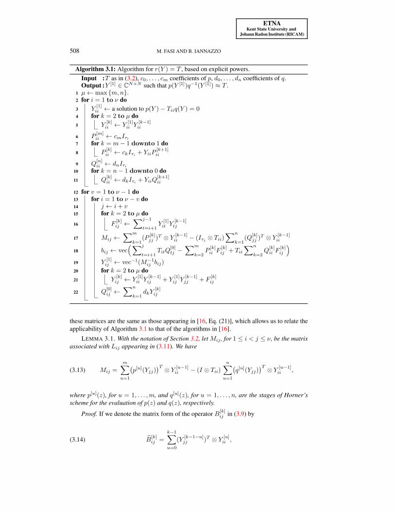
these matrices are the same as those appearing in [16, Eq. (21)], which allows us to relate theapplicability of Algorithm 3.1 to that of the algorithms in [16].

LEMMA 3.1. With the notation of Section 3.2, let Mij , for 1 ≤ i < j ≤ ν, be the matrixassociated with Lij appearing in (3.11). We have

(3.13) Mij =

m∑u=1

(p[u](Yjj)

)T ⊗ Y [u−1]ii − (I ⊗ Tii)

n∑u=1

(q[u](Yjj)

)T ⊗ Y [u−1]ii ,

where p[u](z), for u = 1, . . . ,m, and q[u](z), for u = 1, . . . , n, are the stages of Horner’sscheme for the evaluation of p(z) and q(z), respectively.

Proof. If we denote the matrix form of the operator B[k]ij in (3.9) by

(3.14) B[k]ij =

k−1∑u=0

(Y[k−1−u]jj )T ⊗ Y [u]

ii ,


http://www.kent.edu





then we can rewrite Lij(Yij) in matrix form as Mijvec(Yij), where

(3.15) Mij :=

m∑k=1

ckB[k]ij − Tii

n∑k=1

dkB[k]ij .

On the other hand, we have that

(3.16)

m∑k=1

ckB[k]ij =

m∑k=1

ck

k−1∑u=0

(Y[k−1−u]jj )T ⊗ Y [u]

ii

=

m−1∑u=0

(m∑

k=u+1

ckY[k−1−u]jj

)T⊗ Y [u]

ii

=

m∑u=1

(p[u](Yjj)

)T ⊗ Y [u−1]ii ,

and similarly that

(3.17)n∑k=1

dkB[k]ij =

n∑u=1

(q[u](Yjj)

)T ⊗ Y [u−1]ii .

Plugging (3.16) and (3.17) into (3.15) concludes the proof.Applicability. If T is the triangular factor of a complex Schur decomposition, then all

diagonal blocks have size 1, and the diagonal elements of Y can be computed by solving ascalar equation. If T is in real Schur form, then the diagonal blocks have size at most 2, andthe 2× 2 diagonal blocks of Y can be determined by using, for example, a direct formula asin [16, Prop. 15].

For the complex Schur form, Mij is the same as ψij in [16, Eq. (12)], and the applicabilityof the algorithm depends on what solutions to the scalar equation p(Y ) = Tiiq(Y ) are chosenfor i = 1, . . . , ν.

THEOREM 3.2. Let r = p/q be a rational function with p ∈ Cm[z] and q ∈ Cn[z]coprime. Let T ∈ CN×N be upper triangular, and let ξ1, . . . , ξN ∈ C be such that r(ξi) = tiifor i = 1, . . . , N . Then the two conditions are equivalent:

(a) Algorithm 3.1 with the choice Yii = ξi is applicable to the equation r(Y ) = T , thatis, equation (3.12) has a unique solution Yij for 1 ≤ i < j ≤ N ;

(b) r[ξi, ξj ] 6= 0, for 1 ≤ i < j ≤ N .If either condition is satisfied, then the solution Y is primary and isolated.

Proof. By [16, Lemma 11] we can express the divided differences of p for a, b ∈ C interms of the stages of Horner’s method as p[a, b] =

∑m

j=1aj−1p[j](b). This can be used in

the scalar version of (3.13) to show that

Mij = p[Yii, Yjj ]− Tiiq[Yii, Yjj ] = r[ξi, ξj ]q(ξj).

Since q(ξj) 6= 0 by hypothesis, we have that Mij 6= 0 if and only if r[ξi, ξj ] 6= 0.When either of these conditions is fulfilled, we are in the hypotheses of [16, Thm. 6], and

the solution is primary and isolated.A consequence of Lemma 3.1 is the following result on the existence of isolated solutions

to (1.1).THEOREM 3.3. Let r = p/q be a rational function with p ∈ Cm[z] and q ∈ Cn[z]

coprime, and let A ∈ CN×N . There exists a unique solution X ∈ CN×N to r(X) = A with


http://www.kent.edu





eigenvalues ξ1, . . . , ξN if and only if r(ξ1), . . . , r(ξN ) are the eigenvalues of A (counted withmultiplicities) and r[ξi, ξj ] 6= 0 for 1 ≤ i < j ≤ N . Moreover, X is primary and isolated.

Proof. Let X be a solution with eigenvalues ξ1, . . . , ξN , then the eigenvalues of r(X) arer(ξ1), . . . , r(ξN ) [22]. From [16, Thm. 6], we know that if there exists a unique solution witha given set of eigenvalues, then r[ξi, ξj ] 6= 0 for i 6= j and X is primary and isolated.

Let U∗AU = T be the triangular factor of the complex Schur form of A ordered sothat tii = r(ξi), for i = 1, . . . , N . Since r[ξi, ξj ] 6= 0, we have that Algorithm 3.1 isapplicable to r(Y ) = T and gives a solution Y , which in turn provides X = UY U∗ assolution to r(X) = A. By [16, Thm. 6], X is primary, isolated, and is the unique solutionwith eigenvalues ξ1, . . . , ξN .

We stress that the result in Theorem 3.3 is stronger than that in [16, Cor. 14] as the latterrequires, as a hypothesis, the existence of a solution with the given eigenvalues.

The case of blocks of arbitrary size can be addressed analogously with the differencethat if a non-isolated solution is chosen for any of the block equations p(Y )− Tiiq(Y ) = 0,then the solution produced by the algorithm, when applicable, may be non-isolated or evennon-primary.

THEOREM 3.4. Let r = p/q be a rational function with p ∈ Cm[z] and q ∈ Cn[z]coprime, and let T = (Tij) ∈ CN×N be block upper triangular with ν diagonal blocks of sizeτ1, . . . , τν . Let Ξi ∈ Cτi×τi , for i = 1, . . . , ν, be a solution to r(Ξ) = Tii with eigenvaluesξi1, . . . , ξiτi . Then the two conditions are equivalent:

(a) Algorithm 3.1 with the choice Yii = Ξi is applicable to the equation r(Y ) = T , thatis, equation (3.12) has a unique solution Yij for 1 ≤ i < j ≤ ν;

(b) r[ξiki , ξjkj ] 6= 0, for ξiki an eigenvalue of Ξi and ξjkj an eigenvalue of Ξj , for1 ≤ i < j ≤ ν, 1 ≤ ki ≤ τi, 1 ≤ kj ≤ τj .

If Ξi is an isolated solution to the equation r(X) = Tii for i = 1, . . . , ν, and either of theconditions above is satisfied, then Algorithm 3.1 computes an isolated solution.

Proof. Let ξi1, . . . , ξiτi and ξj1, . . . , ξjτj be the eigenvalues of Yii and Yjj , respectively.If Ui and Uj are unitary matrices such that U∗i YiiUi and U∗j Y

TjjUj are upper triangular, then

Tii := U∗i TiiUi = r(U∗i YiiUi) is upper triangular as well, and so is (U∗j ⊗U∗i )Mij(Uj ⊗Ui)whose diagonal entries (eigenvalues) are

m∑k=1

p[k](ξjkj )ξk−1iki− r(ξiki)

n∑k=1

q[k](ξjkj )ξk−1iki

= r[ξiki , ξjkj ]q(ξjkj ).

By hypothesis we have that q(ξjkj ) 6= 0, thusMij is nonsingular if and only if r[ξiki , ξjkj ] 6= 0for any ki and kj . If Ξi is isolated, then r[ξia, ξib] 6= 0 for 1 ≤ a ≤ τi and 1 ≤ b ≤ τiwith a 6= b. This condition together with Theorem 3.4(b) implies that r[ζi, ζj ] 6= 0 for1 ≤ i < j ≤ N , where ζ1, . . . , ζN are the eigenvalues of the computed solution Y , which isisolated by [16, Thm. 6].

The case in whichA is real and the real Schur form ofA is used can be seen as a particularcase of Theorem 3.4, where the diagonal blocks are of size 1× 1 or 2× 2.

Computational cost. We now discuss the cost of Algorithm 3.1 for the triangular caseν = N and τi = 1, for i = 1, . . . , N . When T presents nontrivial diagonal blocks, the resultsare similar with operations counted at the block instead of the scalar level.

Asymptotically, the most expensive quantities to compute are the µ− 1 sums on line 16,which are related to the stages of the recursion (3.6), and the first sum on line 18, which corre-sponds to the final inversion q(Y )−1p(Y ). Each of these stages entails, for 1 ≤ i < j ≤ N , a


http://www.kent.edu





sum of the type

(3.18) σij :=

j−ε∑t=i+1

aitbtj ,

where ε is either zero or one and ait and btj are scalars for t = i+ 1, . . . , j− ε. Evaluating σijrequires (j − i− ε) multiplications and (j − i− ε− 1) sums, thus 1

3N3 + o(N3) operations

are needed to compute all the σij , for 1 ≤ i < j ≤ N . As these are the only expressionswhose cost is cubic in N , Algorithm 3.1 requires µ

3N3 + o(N3) operations.

Note that evaluating a rational function of order [m/n] at a triangular matrix argument ofsize N via explicit powering has cost µ3N

3 + o(N3), which is exactly the same as that of oursubstitution algorithm.

Since computing the Schur decomposition and recovering the result require 25N3 and3N3 flops, respectively, the asymptotic cost of solving the general equation (1.1) usingAlgorithm 3.1 is

(28 + µ

3

)N3 + o(N3) flops.

3.3. Algorithm based on the Paterson–Stockmeyer method. Let Y be a block uppertriangular solution to (3.1) that has the same block structure as T . Using the Paterson–Stockmeyer evaluation scheme, we can construct, for 1 ≤ i < j ≤ ν, the matrix equationLij(Yij) = bij , where Lij is linear with respect to the block Yij and both Lij and bij canbe computed by using blocks of Y and T such that the difference between the column androw index is greater than j − i, which again we treat as known quantities. We will use theseequations to deduce an algorithm to solve (3.1) that is cheaper than Algorithm 3.1.

The first step is to construct a recursion with one stage for each matrix multiplica-tion in the Paterson–Stockmeyer scheme. We start from the block (i, j) of the equationp(Y )− Tq(Y ) = 0, which reads

p(Y )ij − Tiiq(Y )ij −j∑

t=i+1

Titq(Y )tj = 0.

Since only the first two summands on the left-hand side depend on Yij while the third canbe treated as a known quantity, we need to deduce expressions for p(Y )ij and q(Y )ij thatinvolve only Yij and known quantities. We will give a detailed derivation of the expressionfor p(Y )ij , which is based on the sequence P [k](Y ) defined in (2.3) and the sequence Y [k]

defined in (3.6). The corresponding expression for q(Y )ij can be deduced in a similar manner.It can be shown that2

(3.19) p(Y )ij =

r∑k=0

Y ksii Ck(Y )ij +

r−1∑k=0

Y ksii Y[s]ij P

[k+1](Yjj) +

r−1∑k=0

Y ksii Ψ[k]ij ,

with

Ψ[k]ij :=

j−1∑t=i+1

Y[s]it P

[k+1](Y )tj , k = 0, . . . , r − 1.

2In fact, by an induction argument one can prove that the formula

p(Y )ij = Y dsii P[d](Y )ij +

d−1∑k=0

Y ksii (Ck(Y )ij + Y[s]ij P

[k+1](Yjj) + Ψ[k]ij ),

which coincides with (3.19) for d = r, holds for d = 0, . . . , r − 1 as well.


http://www.kent.edu





In order to get an equation in terms of Yij and known quantities only, we note the thirdsummand on the right-hand side of (3.19) contains only known quantities, while Y [s]

ij andCk(Y )ij can be further reduced as we now explain. From (3.10) we obtain(3.20)

r∑k=0

Y ksii Ck(Y )ij =

r∑k=0

Y ksii

s−1∑′

`=1

c`+skB[`]ij (Yij) +

r∑k=0

Y ksii

s−1∑′

`=2

c`+skΦ[`]ij ,

r−1∑k=0

Y ksii Y[s]ij P

[k+1](Yjj) =

r−1∑k=0

Y ksii B[s]ij (Yij)P

[k+1](Yjj) +

r−1∑k=0

Y ksii Φ[s]ij P

[k+1](Yjj),

with

(3.21) Φ[k]ij :=

k−2∑u=0

Y uiiF[k−u]ij , k = 1, . . . , s,

where F [k]ij is defined in (3.7). Therefore, the last sum on the right-hand side of both equations

in (3.20) contains only known quantities.A similar reduction holds for q(Y )ij , and we get the equation L′ij(Yij) = b′ij , where

b′ij : =

j∑t=i+1

Titq(Y )tj −r∑

k=0

Y ksii

s−1∑′

`=2

c`+skΦ[`]ij −

r−1∑k=0

Y ksii

(Φ

[s]ij P

[k+1](Yjj) + Ψ[k]ij

)

+ Tii

r∑k=0

Y ksii

s−1∑′

`=2

d`+skΦ[`]ij + Tii

r−1∑k=0

Y ksii

(Φ

[s]ij Q

[k+1](Yjj) + Ψ[k]ij

),

with

Ψ[k]ij =

j−1∑t=i+1

Y[s]it Q

[k+1](Y )tj , k = 0, . . . , r − 1,

and the matrix representing L′ij in the vec-basis is

M ′ij = Pij − (Iτj ⊗ Tii)Pij ,(3.22)

where

Pij :=

r∑k=0

(Iτj ⊗ Y ksii )

s−1∑′

`=1

c`+skB[`]ij +

r−1∑k=0

((P [k+1](Y )jj)

T ⊗ Y ksii)B

[s]ij ,

Pij :=

r∑k=0

(Iτj ⊗ Y ksii )

s−1∑′

`=1

d`+skB[`]ij +

r−1∑k=0

((Q[k+1](Y )jj)

T ⊗ Y ksii)B

[s]ij .

(3.23)

As before, these relations lead to an algorithm for computing Y : we can first compute thediagonal blocks of Y (either recursively or by a direct method) and then obtain the others, onesuper-diagonal at a time, by exploiting the relation Yij = vec−1(M−1

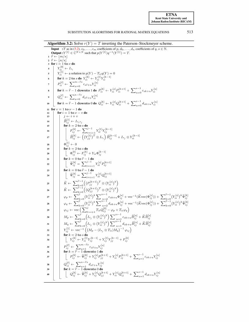
ij vec(bij)).The pseudocode of the algorithm based on the Paterson–Stockmeyer approach is given in

Algorithm 3.2. In order to reduce the overall computational cost of that method, note that B[k]ij


http://www.kent.edu





Algorithm 3.2: Solve r(Y ) = T inverting the Paterson–Stockmeyer scheme.Input :T as in (3.2), c0, . . . , cm coefficients of p, d0, . . . , dn coefficients of q, s ∈ N.Output :Y [1] ∈ CN×N such that p(Y [1])q−1(Y [1]) = T .

1 r ← bm/sc2 r ← bn/sc3 for i = 1 to ν do4 Y

[0]ii ← Iτi

5 Y[1]ii ← a solution to p(Y )− Tiiq(Y ) = 0

6 for k = 2 to s do Y[k]ii ← Y

[1]ii Y

[k−1]ii

7 P[r]ii ←

∑m−rs

u=0csr+uY

[u]ii

8 for k = r − 1 downto 1 do P[k]ii ← Y

[s]ii P

[k+1]ii +

∑s−1

u=0csk+uY

[u]ii

9 Q[r]ii ←

∑n−rs

u=0dsr+uY

[u]ii

10 for k = r − 1 downto 0 do Q[k]ii ← Y

[s]ii Q

[k+1]ii +

∑s−1

u=0dsk+uY

[u]ii

11 for v = 1 to ν − 1 do12 for i = 1 to ν − v do13 j ← i+ v

14 B[1]ij ← Iτiτj

15 for k = 2 to s do16 F

[k]ij ←

∑j−1

t=i+1Y

[1]it Y

[k−1]tj

17 B[k]ij ←

((Y

[1]jj

)T ⊗ Iτi) B[k−1]ij + Iτj ⊗ Y

[k−1]ii

18 Φ[1]ij ← 0

19 for k = 2 to s do20 Φ

[k]ij ← F

[k]ij + YiiΦ

[k−1]ij

21 for k = 0 to r − 1 do22 Ψ

[k]ij =

∑j−1

t=i+1Y

[s]it P

[k+1]tj

23 for k = 0 to r − 1 do24 Ψ

[k]ij =

∑j−1

t=i+1Y

[s]it Q

[k+1]tj

25 K ←∑r−1

k=0

((P

[k+1]jj

)T ⊗ (Y [s]ii

)k)26 K ←

∑r−1

k=0

((Q

[k+1]jj

)T ⊗ (Y [s]ii

)k)27 ϕp ←

∑r

k=0

(Y

[s]ii

)k∑′s−1

u=2csk+uΦ

[u]ij + vec−1(Kvec(Φ

[s]ij )) +

∑r−1

k=0

(Y

[s]ii

)kΨ

[k]ij

28 ϕq ←∑r

k=0

(Y

[s]ii

)k∑′s−1

u=2dsk+uΦ

[u]ij + vec−1(Kvec(Φ

[s]ij )) +

∑r−1

k=0

(Y

[s]ii

)kΨ

[k]ij

29 ϕij ← vec(∑j

t=i+1TitQ

[0]tj − ϕp + Tiiϕq

)30 Mp ←

∑r

k=0

(Iτj ⊗

(Y

[s]ii

)k)∑′s−1

u=1csk+uB

[u]ij + KB

[s]ij

31 Mq ←∑r

k=0

(Iτj ⊗

(Y

[s]ii

)k)∑′s−1

u=1dsk+uB

[u]ij + KB

[s]ij

32 Y[1]ij ← vec−1

((Mp − (Iτj ⊗ Tii)Mq

)−1ϕij

)33 for k = 2 to s do34 Y

[k]ij ← Y

[1]ii Y

[k−1]ij + Y

[1]ij Y

[k−1]jj + F

[k]ij

35 P[r]ij ←

∑m−rs

u=1csr+uY

[u]ij

36 for k = r − 1 downto 1 do37 P

[k]ij ← Ψ

[k]ij + Y

[s]ij P

[k+1]jj + Y

[s]ii P

[k+1]ij +

∑s−1

u=1csk+uY

[u]ij

38 Q[r]ij ←

∑n−rs

u=1dsr+uY

[u]ij

39 for k = r − 1 downto 0 do40 Q

[k]ij ← Ψ

[k]ij + Y

[s]ij Q

[k+1]jj + Y

[s]ii Q

[k+1]ij +

∑s−1

u=1dsk+uY

[u]ij


http://www.kent.edu





in (3.14) and Φ[k]ij in (3.21) can be computed recursively by exploiting the identities

Φ[k]ij =

F

[2]ij , k = 2,

F[k]ij + YiiΦ

[k−1]ij , k = 3, . . . , s,

B[k]ij =

Iτiτj , k = 1,((Y

[1]jj

)T ⊗ Iτi) B[k−1]ij + Iτj ⊗ Y

[k−1]ii , k = 2, . . . , s.

The computational cost can be further reduced by using the identities

vec( r−1∑k=0

Y ksii Φ[s]ij P

[k+1](Yjj))

=

r−1∑k=0

((P [k+1](Y )jj)

T ⊗ Y ksii)

vec(Φ

[s]ij

),

vec( r−1∑k=0

Y ksii Φ[s]ij Q

[k+1](Yjj))

=

r−1∑k=0

((Q[k+1](Y )jj)

T ⊗ Y ksii)

vec(Φ

[s]ij

).

Indeed, the sums on the left-hand side appear in the expression for b′ij while those on theright-hand side appear in (3.22). Thus, it is more convenient to compute them only once at thebeginning of the iteration and reuse them when needed later on.

Applicability. We show that M ′ij in (3.22) is the same as Mij in (3.13), which impliesthat Algorithm 3.2 is applicable if and only if Algorithm 3.1 is.

LEMMA 3.5. For the matrix M ′ij in (3.22), with 1 ≤ i < j ≤ ν, we have that

M ′ij =

m∑k=1

ckB[k]ij − (Iτj ⊗ Tii)

n∑k=1

dkB[k]ij ,

that is, M ′ij is the same as Mij in (3.13).Proof. We prove that M ′ij = Mij by showing for the matrices in (3.23) that

Pij =

m∑k=0

ckB[k]ij and Pij =

m∑k=0

dkB[k]ij .

With B[0]ij = 0, the first summand of Pij can be written as

r∑k=0

s−1∑′

`=0

c`+sk(Iτj ⊗ Y ksii )B[`]ij ,

while for the second we haver−1∑t=0

(P [t+1](Yjj))T ⊗ Y tsii )B

[s]ij

=

r−1∑t=0

(( r∑k=t+1

s−1∑′

`=0

c`+skY`+s(k−t−1)jj

)T⊗ Y tsii

) s−1∑v=0

(Y s−1−vjj )T ⊗ Y vjj

=

r∑k=1

s−1∑′

`=0

c`+sk

k−1∑t=0

s−1∑v=0

((Y `+sk−1−st−vjj )T ⊗ Y st+vii

)=

r∑k=1

s−1∑′

`=0

c`+sk

sk−1∑u=0

((Y `+sk−1−ujj )T ⊗ Y uii

)=

r∑k=1

s−1∑′

`=0

c`+sk((Y `jj)

T ⊗ Iτi)B

[sk]ij .


http://www.kent.edu





The fact that Pij =∑m

k=0ckB

[k]ij follows from the identity

(3.24) (Iτj ⊗ Y ksii )B[`]ij + ((Y `jj)

T ⊗ Iτi)B[sk]ij = B

[`+sk]ij ,

which holds for ` = 0, . . . , s − 1 when k < r and for ` = 0, . . . ,m − rs when k = r.Equation (3.24) is a special case of the more general identity

(Iτj ⊗ Y aii )B[b]ij + ((Y bjj)

T ⊗ Iτi)B[a]ij = B

[a+b]ij , a, b > 0,

whose proof is immediate.A similar argument shows that Pij =

∑n

k=0dkB

[k]ij , and this concludes the proof of the

lemma.In view of Lemma 3.5, Algorithm 3.2 is applicable if and only if Algorithm 3.1 is, thus

Theorem 3.3 and Theorem 3.4 hold for Algorithm 3.2 with the same hypotheses.Computational cost. As done in the previous section, we discuss the cost of Algorithm 3.2

for the case ν = N and τi = 1 for i = 1, . . . , N .Note that the coefficient of N3 in the computational cost is obtained by counting, for all

1 ≤ i < j ≤ N , the number of sums of the type (3.18) appearing in the pseudocode. Evalu-ating each of these sums requires 1

3N3 + o(N3) operations, and their number is exactly the

same as that of the matrix multiplications and inversions needed in the Paterson–Stockmeyerevaluation scheme, that is, r + r + s. Indeed the most expensive operations in the algorithmare: the sum on line 16, which is repeated s− 1 times and is related to the recursion (3.4); thetwo sums on lines 22 and 24, which correspond to the evaluation of Ck(A) and Dk(A) and areperformed r and r times, respectively; and the sum on line 29, which is the counterpart of thefinal inversion in q(Y )−1p(Y ). Therefore, the total cost of Algorithm 3.2 is r+r+s3 N3+o(N3)flops, and the asymptotic cost of of solving the general equation (1.1) using Algorithm 3.2 is(28 + r+r+s

3

)N3 + o(N3) flops.

4. Numerical experiments. We compare experimentally the performance of Algo-rithm 3.1, Algorithm 3.2, and [16, Alg. 1] and give an example showing how these canbe used to approximate matrix functions defined implicitly via matrix equations.

The experiments were run in MATLAB 2019a (version 9.6) on a machine equipped withan Intel I5-5287 processor running at 2.90GHz. We compare the following codes for thesolution of rational matrix equations.

• invrat_horn, an implementation of [16, Alg. 1];• invrat_pow, an implementation of Algorithm 3.1 based on the complex Schur

decomposition;• invrat_ps, an implementation of Algorithm 3.2 based on the complex Schur de-

composition.The implementations we used to perform the experiments in this section are available on theMATLAB Central File Exchange.3

We evaluate the stability of our algorithms by comparing the 1-norm forward error of thecomputed solutions with the quantity κf−1(A)u, where u = 2−53 is the unit roundoff of IEEEdouble precision arithmetic, and κf−1(A) is the 1-norm condition number of the solution tof(X) = A for a specific choice of f−1. Numerically, we estimate κf−1(A) by means of thefunction funm_condest1 from the Matrix Function Toolbox [20], and the forward error bycomputing in double precision the quantity

eA =‖XA −X‖1‖X‖1

,

3https://mathworks.com/matlabcentral/fileexchange/74317.


http://www.kent.edu


https://mathworks.com/matlabcentral/fileexchange/74317




0 20 40 6010−18

10−13

10−8

10−3

κr−1(A)uinvrat_horninvrat_powinvrat_ps

(a) Forward error.

2 4 6 8

0.6

0.8

1

η

invrat_horninvrat_powinvrat_ps

(b) Performance profile for (a).

FIG. 4.1. Left: relative forward error of invrat_horn, invrat_pow, and invrat_ps for the matrices in thetest set sorted by descending condition number κr−1 (A). Right: corresponding performance profile.

where XA is the solution computed by algorithm A and X is a reference solution.

4.1. Numerical stability. In this first experiment, we assess the stability of the proce-dures invrat_horn, invrat_pow, and invrat_ps by performing an experiment similarto [16, Test 1]. As the order of the rational function used there is too low to show any remark-able difference among the three algorithms, we turn to a rational function of higher order andconsider the [5/5] Padé approximant to the exponential. The reference solution is obtainedby running invrat_pow with 113 significant binary digits of accuracy, which correspondsto IEEE binary128 floating point arithmetic [25, Table 3.2]. In order to work with preci-sion higher than double, we rely on the overloaded methods of the Advanpix MultiprecisionComputing Toolbox [1] (version 4.4.7.12739).

In Figure 4.1a, we compare the 1-norm forward error of the three algorithms for the sametest as in [16, Test 1], which contains 63 nonnormal matrices of size 10 with no nonpositivereal eigenvalues. We do not consider normal matrices, for which the triangular Schur factor isin fact diagonal, as invrat_horn, invrat_pow, and invrat_ps all reduce to diagonalizationin that case. The fact that the forward error is always approximately bounded by κr−1(A)usuggests that the three implementations behave in a forward stable fashion. Note that thealgorithms attain a remarkably similar accuracy for most matrices, and when that is not thecase, the difference among the performance of the three methods is marginal.

Figure 4.1b presents the same data by means of a performance profile [12]. In the plot, theheight of the line corresponding to algorithm A at η = η0 represents the fraction of matricesin the test set on which the 1-norm relative forward error of A is at most η0 times that of thealgorithm that gives the most accurate result. The figure confirms that the accuracy of thethree algorithms on our test set is very similar, but invrat_ps appears to be, overall, slightlymore accurate than the two alternative approaches.

In order to draw more general results, we conducted a second experiment. For each pair ofdistinct implementations A and B, we tried to find the 5× 5 matrix A and, for different valuesof m, the [m/m] rational function r that maximize the ratio eA/eB when the two algorithmsA and B are used to solve (1.1). As optimization method, we used the multidirectional searchmethod of Dennis and Torczon [11], implemented in the mdsmax function of the MatrixComputation Toolbox [19].


http://www.kent.edu





TABLE 4.1Maximum ratio of forward errors for all possible pairs of algorithms. The optimization procedure tries to

determine a 5× 5 matrix and the coefficients of the numerator and denominator of a [m/m] rational function r thatmaximize eA/eB . Each cell contains four values corresponding to the cases m = 3 (top left), m = 5 (top right),m = 7 (bottom left), and m = 9 (bottom right).

A Binvrat_horn invrat_pow invrat_ps

invrat_horn – – 3.20 1.37 1.95 2.32– – 1.53 1.73 1.42 1.61

invrat_pow 1.20 1.77 – – 71.53 2.371.37 2.92 – – 2.74 1.29

invrat_ps 2.24 1.33 35.37 2.29 – –1.59 2.16 1.51 2.25 – –

In Table 4.1, we report these ratios for the four cases m = 3, 5, 7, and 9, which appear inthe top left, top right, bottom left, and bottom right corners, respectively, of every cell. Theresults show that the three algorithms tend to behave similarly, as the forward error of onealgorithm does not exceed that of any other by more than one order of magnitude in mostcases.

We conclude that the three algorithms do not differ much in terms of accuracy, and thattheir good stability properties make them reliable enough to be of practical use.

4.2. Computational time. Figure 4.2 shows how the execution time required by the algo-rithms invrat_horn, invrat_pow, and invrat_ps to solve the matrix equation r(X) = Adepends on the size of the matrix A and on the order of the rational function r.

As the analysis of the computational cost shows, the time required to compute the Schurdecomposition of the input matrix tends to be preponderant for rational functions of low order,thus we prefer not to take it into account and to feed the algorithm matrices that are already inupper triangular form. As the number of operations which the algorithms carry out dependson the number of nonzeros in the matrix but not on their numerical value, we use the 0-1matrix A ∈ CN×N with aij = 1 for 1 ≤ i ≤ j ≤ N . A similar observation can be made forthe coefficients of the rational functions, which we draw from a Gaussian distribution. Theexecution time is estimated by means of the MATLAB function timeit.

In Figure 4.2a, we fix the order of the rational function to 25 and let the size of the matrixincrease from 10 to 400. The time required by the three algorithms rises more than linearly.For matrices of order 20 or more, invrat_horn is the slowest algorithm, invrat_pow isthe fastest for matrices of size smaller than 50, whereas invrat_ps is the fastest for largermatrices. This is in line with the analysis of the computational cost.

In Figure 4.2b the algorithms are run for matrices of size 250 using rational functions oforders between 3 and 100. As expected, the execution time of invrat_horn and invrat_powgrows linearly with the order of the approximant, and the latter is always the fastest of the two.The execution time of invrat_ps, on the other hand, grows sublinearly, again following theanalysis of the computational cost. The results for complex matrices with complex coefficientsare qualitatively analogous.

4.3. Computing the Lambert W function. In order to illustrate how these algorithmscan be employed to solve more general matrix equations of the form f(X) = A wheref is a primary matrix function, we consider the computation of the matrix Lambert Wfunction [10] defined implicitly as any solution to the equation XeX = A, which is of interest


http://www.kent.edu





0 100 200 300 40010−4

10−3

10−2

10−1

100

101

N

s


(a) m = 25.

0 20 40 60 80 1000

1

2

m

s


(b) N = 250.

FIG. 4.2. Execution time (in seconds) of invrat_horn, invrat_pow, and invrat_ps on matrices of increas-ing size N (left) and rational functions of increasing order m (right).

in the analysis of the stability of delay differential equations [4, 8, 18, 27]. The inverse ofthe real function [−1/e,∞] → R : x → xex can be extended analytically to a functionW0(z) : C \ (−∞, 1/e)→ C, which is said to be the 0th branch of the Lambert W function.

For computing W0(A), we compare:

• lambertwm, an implementation of [15, Alg. 1];• lambertwm_rat, an algorithm that uses invrat_ps to solve r(X) = A, where r

is a diagonal Padé approximant to xex. In our experiments, we found that 28 isthe lowest optimal degree for the Paterson–Stockmeyer method [14] that providessufficient accuracy for all the matrices in the test set we consider.

Following the well-established paradigm of recomputing the diagonal of functions ofupper triangular matrices in a direct way [2, 3], in lambertwm_rat we recompute the diagonalelements of Y using a direct formula. More precisely, if we were to follow the approachin Algorithms 3.1 and 3.2 exactly, after reducing the problem to the triangular form (1.2),we would obtain the diagonal blocks of Y by choosing the solution to r(X) = Tii that bestapproximates W0(Tii). Instead, we set Yii = W0(Tii) and continue the recursion using thisvalue in lieu of r−1(Tii). The off-diagonal blocks are still computed by substitution. Themain advantage of this technique is that we do not need to solve smaller matrix equationfor non-trivial diagonal blocks. Moreover, our results show that this strategy leads to moreaccurate solutions in some cases.

This modification can be seen as applying Algorithms 3.1 and 3.2 to the matrix equationr(Y ) = T , where T coincides with T except for the diagonal blocks, since Tii is replaced bythe block Tii such that r−1(Tii) = W0(Tii). When W0(Tii) is a 2× 2 block arising from thereal Schur decomposition, we use [16, Prop. 15].

We compare the performance of lambertwm and lambertwm_rat for the test set usedin [15, Exp. 2], which contains 47 matrices of size 10 taken from the MATLAB gallery.As lambertwm is an iterative method, it cannot be easily extended to multiprecision, and tocompute our reference solution we adopt the same algorithm used in [15, Exp. 2], whichdiagonalizes the matrix in higher precision by using the eig function provided by the SymbolicMath Toolbox [32].


http://www.kent.edu





0 5 10 15 20 25 30 35 40 4510−17

10−13

10−9

10−5

κW0(A)u

lambertwmlambertwm_rat

(a) Forward error.

1 2 3 4 5

0.4

0.6

0.8

1

η

lambertwmlambertwm_rat

(b) Performance profile for (a).

0 20 400

5

10

(c) Cost ratio.

FIG. 4.3. Top: forward error of lambertwm and lambertwm_rat for the matrices in the test set sorted bydescending condition number κW0 (A). Bottom left: corresponding performance profile. Bottom right: ratio of theestimated computational costs of lambertwm and lambertwm_rat.

Figure 4.3a compares the 1-norm forward error of lambertwm and lambertwm_rat withthe quantity κW0(A)u, and Figure 4.3b presents the same data by means of performanceprofiles. The results suggest that both algorithms behave in a forward stable way and achieveremarkably similar accuracy for most matrices in the test set. The algorithm lambertwm_ratachieves slightly higher accuracy for about a quarter of the matrices in the data set, whichjustifies the more favorable curves of this algorithm in the performance profile.

In Figure 4.3c, we compare the leading terms of the computational cost of the twoimplementations for the matrices in the test set. In both cases, 28N3 flops are required tocompute the Schur decomposition and recovering the result at the end of the computation. Theadditional cost of lambertwm_rat depends only on the size of the matrix and on the order ofthe rational approximant and can be easily seen to be 13N3/3. On the other hand, lambertwmsplits the matrix into two blocks and performs a few steps of the Newton method for eachblock. In assessing the flop count, we took into account the number of matrix multiplications,inversions, and square roots needed to compute the starting value and perform the requiredsteps of the Newton method and the cost for the solution of the ensuing Sylvester equation


http://www.kent.edu





by means of the Bartels–Stewart algorithm [5]. We ignored the cost of ordering the Schurdecomposition so that the eigenvalues appear along the diagonal of the triangular Schur factorin two clusters. The results show that, in the test set that we considered, the new algorithm isup to eleven times faster than lambertwm, and the speedup reaches a factor seven for morethan half of the matrices in the test set.

These differences are not as apparent in our MATLAB implementations, where the gain oflambertwm_rat over lambertwm is limited. This is not surprising: the former method mostlycomprises element-wise operations that are interpreted by MATLAB at runtime, whereas thelatter is rich in matrix multiplications and inversions, kernels for which MATLAB relies onhighly optimized C and Fortran libraries.

As we use the Padé approximant centered at 0, the accuracy of this algorithm deterioratesfor matrices with large eigenvalues. In order to make the new algorithm a reliable alternativeto lambertwm, this case has to be addressed. This will be the subject of future work.

5. Conclusions. We developed two new algorithms for solving rational matrix equationsthat are more efficient than existing algorithms for the same problem. These new techniquesinvert two customary methods for the evaluation of rational matrix functions, one based onthe explicit powering technique and the other on the Paterson–Stockmeyer algorithm. Ourexperiments suggest that the new techniques are as accurate as existing alternatives: this isconsistent with the error analysis of similar algorithms for the square root and pth root, aswell as with the stability of the corresponding methods for the evaluation of rational matrixfunctions, which are all equivalently stable [22, Thm. 4.5]. We characterized the applicabilityof substitution algorithms for rational matrix equations in a way that feels more natural thanprevious attempts in the literature [16].

General functional matrix equations such as those that define the matrix logarithm or thematrix Lambert W function can be reduced to rational form by means of rational approxima-tion. We briefly discussed how this strategy can be exploited to develop a naïve method forcomputing the Lambert W function that, in a number of cases, is more accurate and efficientthan the reference algorithm [15]. An analogous strategy for the matrix logarithm or the inversesine and cosine functions would not provide an advantage over the current state-of-the-artalgorithms.

Nevertheless, the diagonal Padé approximants to the exponential, sine, and cosine allshow symmetries in their coefficients. If these patterns were exploited, one could in principledeliver faster substitution algorithms tailored to the solution of specific problems. We intendto investigate this in future work.

REFERENCES

[1] ADVANPIX, Multiprecision Computing Toolbox, Advanpix, Tokyo.http://www.advanpix.com

[2] A. H. AL-MOHY AND N. J. HIGHAM, A new scaling and squaring algorithm for the matrix exponential,SIAM J. Matrix Anal. Appl., 31 (2009), pp. 970–989.

[3] , Improved inverse scaling and squaring algorithms for the matrix logarithm, SIAM J. Sci. Comput., 34(2012), pp. C153–C169.

[4] F. M. ASL AND A. G. UHLSOY, Analysis of a system of linear delay differential equations, J. Dyn. Sys. Meas.Control., 125 (2003), pp. 215–223.

[5] R. H. BARTELS AND G. W. STEWART, Algorithm 432: Solution of the matrix equation AX +XB = C,Comm. ACM, 15 (1972), pp. 820–826.

[6] A. BJÖRCK AND S. HAMMARLING, A Schur method for the square root of a matrix, Linear Algebra Appl.,52/53 (1983), pp. 127–140.

[7] M. BLADT AND M. SØRENSEN, Efficient estimation of transition rates between credit ratings from observa-tions at discrete time points, Quant. Finance, 9 (2009), pp. 147–160.


http://www.kent.edu


http://www.advanpix.com




[8] R. CEPEDA-GOMEZ AND W. MICHIELS, Some special cases in the stability analysis of multi-dimensionaltime-delay systems using the matrix Lambert W function, Automatica J. IFAC, 53 (2015), pp. 339–345.

[9] T. CHARITOS, P. R. DE WAAL, AND L. C. VAN DER GAAG, Computing short-interval transition matrices ofa discrete-time Markov chain from partially observed data, Stat. Med., 27 (2008), pp. 905–921.

[10] R. M. CORLESS, G. H. GONNET, D. E. G. HARE, D. J. JEFFREY, AND D. E. KNUTH, On the Lambert Wfunction, Adv. Comput. Math., 5 (1996), pp. 329–359.

[11] J. E. DENNIS, JR. AND V. TORCZON, Direct search methods on parallel machines, SIAM J. Optim., 1 (1991),pp. 448–474.

[12] E. D. DOLAN AND J. J. MORÉ, Benchmarking optimization software with performance profiles, Math.Program., 91 (2002), pp. 201–213.

[13] J.-C. EVARD AND F. UHLIG, On the matrix equation f(X) = A, Linear Algebra Appl., 162/164 (1992),pp. 447–519.

[14] M. FASI, Optimality of the Paterson-Stockmeyer method for evaluating matrix polynomials and rational matrixfunctions, Linear Algebra Appl., 574 (2019), pp. 182–200.

[15] M. FASI, N. J. HIGHAM, AND B. IANNAZZO, An algorithm for the matrix Lambert W function, SIAM J.Matrix Anal. Appl., 36 (2015), pp. 669–685.

[16] M. FASI AND B. IANNAZZO, Computing primary solutions of equations involving primary matrix functions,Linear Algebra Appl., 560 (2019), pp. 17–42.

[17] F. GRECO AND B. IANNAZZO, A binary powering Schur algorithm for computing primary matrix roots,Numer. Algorithms, 55 (2010), pp. 59–78.

[18] J. M. HEFFERNAN AND R. M. CORLESS, Solving some delay differential equations with computer algebra,Math. Sci., 31 (2006), pp. 21–34.

[19] N. J. HIGHAM, The Matrix Computation Toolbox, Website.http://www.maths.manchester.ac.uk/~higham/mctoolbox

[20] , The Matrix Function Toolbox, Website.http://www.maths.manchester.ac.uk/~higham/mftoolbox

[21] , Computing real square roots of a real matrix, Linear Algebra Appl., 88/89 (1987), pp. 405–430.[22] , Functions of Matrices: Theory and Computation, SIAM, Philadelphia, 2008.[23] N. J. HIGHAM AND L. LIN, An improved Schur-Padé algorithm for fractional powers of a matrix and their

Fréchet derivatives, SIAM J. Matrix Anal. Appl., 34 (2013), pp. 1341–1360.[24] B. IANNAZZO AND C. MANASSE, A Schur logarithmic algorithm for fractional powers of matrices, SIAM J.

Matrix Anal. Appl., 34 (2013), pp. 794–813.[25] IEEE, IEEE Standard for Floating-Point Arithmetic. IEEE Std. 754-2008 (revision of IEEE Std. 754-1985),

The Institute of Electrical and Electronics Engineers, New York, August 2008.[26] R. B. ISRAEL, J. S. ROSENTHAL, AND J. Z. WEI, Finding generators for Markov chains via empirical

transition matrices, with applications to credit ratings, Math. Finance, 11 (2001), pp. 245–265.[27] E. JARLEBRING AND T. DAMM, The Lambert W function and the spectrum of some multidimensional

time-delay systems, Automatica J. IFAC, 43 (2007), pp. 2124–2128.[28] M. S. PATERSON AND L. J. STOCKMEYER, On the number of nonscalar multiplications necessary to evaluate

polynomials, SIAM J. Comput., 2 (1973), pp. 60–66.[29] B. SINGER AND S. SPILERMAN, The representation of social processes by Markov models, Am. J. Sociol., 82

(1976), pp. 1–54.[30] M. I. SMITH, A Schur algorithm for computing matrix pth roots, SIAM J. Matrix Anal. Appl., 24 (2003),

pp. 971–989.[31] T. TAKADA, A. MIYAMOTO, AND S. F. HASEGAWA, Derivation of a yearly transition probability matrix for

land-use dynamics and its applications, Landsc. Ecol., 25 (2009), pp. 561–572.[32] THE MATHWORKS, Symbolic Math Toolbox, Software, The MathWorks, Natick.

http://www.mathworks.co.uk/products/symbolic/


http://www.kent.edu


http://www.maths.manchester.ac.uk/~higham/mctoolbox

http://www.maths.manchester.ac.uk/~higham/mftoolbox

http://www.mathworks.co.uk/products/symbolic/

substitution algorithms for rational matrix equations

Documents