substantive policy statement 0144~000 …azdeq.gov/function/laws/download/2014/leachability guidance...

0144~000 LEACHABILITY GUIDANCE POLICY

Level One Arizona Department~ of :Environmental Quality

Originator: Jean Calhoun, Director Waste Programs Division

contact for Information: Michele Robertson

Issue Date: February '27, 1998

PURPOSE

This policy establishes the guidance document "A screening Method to Determine Soil Concentrations Protective of Groundwater Quality" (commonly known as the leachability guidance) as the recommended approach to satisfy the groundwater quality protection requirement in the Soil Remediation Standards Rule (A.A.C. R18-7-203.B.1).

AUTHORITY

A.R.S. § 49-152.a, A.R.S. §§ 49-221 et. seq., A.A.C. R18-11-401 et seq., and A.A.C. R18-7-203.B.1.

POLICY

All ADEQ programs conducting, reviewing, and/ or approving soil remediations shall apply the procedures in the leachability guidance consistent with the assumptions and limitations described in the document "A · Screening Method to Determine Soil

·Concentrations Protective of Groundwater Quality." (Note: A copy of the document is available at the Information Desk of the Department of Environmental Quality, 3033 North Central Avenue, Phoenix, Arizona.)

RESPONSIBILITY

All managers and supervisors shall be responsible for ensuring that their respective programs follow ·this policy. All staff are · responsible for knowing the limitations of the models used to develop the groundwater protection levels (GPLs) before using the guidance document or the models.

APPLICABILITY

This policy shall apply to all programs administered by ADEQ that are responsible for soil remediation ·activities.

SUBSTANTIVE POLICY STATEMENT

This Substantive Policy statement is advisory only. A substantive policy statement does not include internal procedural documents that only affect the internal procedures of the agency and does not impose additional requirements or penalties on regulated partied or include confidential information or rules made in accordance with the Arizona Administrative Procedure Act. If you believe that this substantive policy statement does impose additional requirements or penalties on regulated parties, you may petition the agency under Arizona Revised Statutes section 41-1033 for a review of the statement.

jc18

Rectangle

0144.000 LEACHABILITY GUIDANCE POLICY

Level one Arizon• Department of Environmental Quality

originator: Jean Calhoun, Director Waste Programs Division

contact for Information:

Issue Date:

Michele Robertson

February 27, 1998

-APPROVED BY:

Arizona Department of Environmental -Quality:

~0-<J,, ItUSSeiiF. Rlloades .

N cy Direct , Air Quality Division

·~

Date

Date

Date

. iJ~Jf. David st. Jo n Manager,

Division

Ed Sadler Director, Water Quality Division Northern Regional

Date

Date

~Won¥7/ff ~~~~~~-'~~61 'i ~ Ma

Manager, Date Southern Regional Office

A-~1--.-iStrative Counsel Date Office of the Administrative Counsel

ARIZONA DEPARTMENT OF ENVIRONMENTAL QUALITY NOTICE OF AGENCY SUBSTANTIVE POLICY STATEMENT

1. Subject of the substantive policy statement and the substantive policy statementnumber by which the policy statement is referenced:

Document Title: Leachability Guidance Policy

Identification number: 0144.000

2. Date the substantive policy statement was issued and the effective date of the policystatement if different from the issuance date:

Date of Document: September, 1996 Effective date of Policy: February 27, 1998

3. Summary of the contents of the substantive policy statement:

This policy establishes the guidance document "A Screening Method to Determine SoilConcentrations Protective of Groundwater Quality" (commonly known as the leachabilityguidance) as the recommended approach to satisfy the groundwater quality protectionrequirement in the Soil Remediation standards Rule (A.A.C. R18-7-203.B.1).

4. A statement as to whether the substantive policy statement is a new statement or arevision:

____New ____Revised __X__Existing

5. The name, address, and telephone number of the person to whom questions andcomments about the substantive policy statement may be directed:

Name: Robin Thomas Address: 1110 W. Washington, Phoenix, AZ 85007 Telephone: 602-771- 4159

6. Information about where a person may obtain a copy of the substantive policystatement and the costs for obtaining the policy statement:

Copies of this policy document are available for download as a PDF document from ADEQ'swebsite, or at the cost of $0.25 per page from ADEQ’s Information Desk, 1110 W.Washington, Phoenix, AZ 85007.

22



http://azdeq.gov/function/laws/download/policy/0144.000.pdf

jc18

Rectangle



jc18

Rectangle

TABLE OF CONTENTS

Page

Executive Summary . . . . . . . . . . . . . . . . . . . . . . . . . . ......... _. . . ... m

Leachability Working Group . . . . . . . . . . . . . . . . . . . . . . . . . . . . . . . . . . vu

List of Tables and Figures . . . . . . . . . . . . . . . . . . . . . . . . .•••• lX

I.

II.

III.

IV.

Introduction .......................................... 1

Approach to Problem . . . . . . . . . . . . . . . . . . . . . . . . . . . . . . . . . . . . 3

Screening Approach for Organic Contaminants .

Screening Approach for Inorganic Contaminants

Appendix A: Description of Modeling Approach .for Organic Contaminants

Appendix B: ADEQ Model Description

Appendix C: Description of Approach for Inorganic Contaminants

1

. .... 5

.... 33

EXECUTIVE SUMMARY

In September 1994, the Arizona Department of Environmental Quality (ADEQ) formed a Cleanup Standards Task Force to establish consistent remediation standards for all programs administered by ADEQ. The Task Force's work led to passage of legislation in 1995, A.R.S. 49-151 and 49-152, which mandated the development of consistent soil remediation standards based on the risk to human health and the environment and required ADEQ to establish these standards in rule. The Interim Soil Remediation Standards Rule (Interim Rule) was certified March 29, 1996.

Under the Interim Rule, a party conducting a soil remediation may use one of two approaches for determining the appropriate soil cleanup standard. The party may simply elect to use Health-Based Guidance Levels (HBGLs) developed by the Arizona Department of Health Services (ADHS) as cleanup standards. Residential and non-residential HBGLs for hundreds of chemicals are listed in.the Interim Rule. Alternatively, a risk assessment may be used to develop site-specific cleanup standards based on either residential or nonresidential use of the property. No matter which approach is selected, the residual concentration of a contaminant in soil cannot (1) cause or threaten contamination of groundwater to exceed the Aquifer Water Quality Standard (A WQS) at a program-specific point of compliance; (2) create a nuisance; (3) cause or threaten to cause a violation of a surface Water Quality Standard; or (4) exhibit the ignitability, corrosivity or reactivity characteristic of hazardous waste.

The Leachability Working Group of the Cleanup Standards Task Force (the Working Group) was assigned the task of developing a screening method to determine if residual contaminant concentrations could cause or threaten to cause contamination of groundwater. In fulfillment of this assignment, the Working Group prepared this report.

Approach for Organic Contaminants

In order to provide a scientific basis for the screening process, the Working Group determined that a contaminant fate-and-transport. model would be needed to calculate potential impacts on groundwater quality due to residual soil contamination. The Working Group evaluated several vadose zone contaminant fate-and-transport models for organic chemicals, eventually selecting a one-dimensional model developed by ADEQ. As opposed to other commonly used vadose zone models, such as VLEACH and SESOIL, the ADEQ model was developed specifically to determine the level of residual contaminant concentrations in soil that would be protective of groundwater quality at a point of compliance in the underlying aquifer. The ADEQ model simulates transport of a contaminant undergoing three-phase partitioning using an analytical approach for the unsaturated zone {based on solutions developed by Dr. William A~ Jury, University of California-Riverside) and a mixing-cell model for the saturated zone. The ADEQ model integrates groundwater transport of organic chemicals, a significant advantage over the other

ill

models reviewed .. Using the ADEQ model, numerous simulations for different organic chemicals were run using conservative, but realistic, default values for the model input parameters. Based on the modeling results, Groundwater Protection Levels ("GPLs"), which are soil cleanup levels protective of groundwater quality, were developed for commonly occurring organic compounds with an A WQS.

Based on evaluation of the model results, three options f<Jr determining GPLs for organic contaminants were developed. As an initial screening step, the list of chemicals present at the cleanup site can be compared with a short list of Drganic compounds with limited mobility in the subsurface. If any of the chemicals is on the short list {Table 2), the threat of groundwater contamination from that chemical is considered negligible and the HBGL or a site-specific risk assessment level may serve as the cleanup standard. For other organic compounds with an AWQS,.Minimum GPLs (Table 3) are provided. The Minimum GPLs are based on a "worst-case" situation (where the whole soil pmfile is contaminated from surface to groundwater). The Minimum GPL can be used as the soil remediation level without detailed site-specific information.

The second and third options require site-specific soU and contaminant characterization. The second screening step requires that the site-specific depth to groundwater and the vertical extent of contamination in the vadose zone be determined. The Working Group developed graphs which provide Alternative GPLs for commonly occurring organic compounds with an AWQS. The graphs show Alternative GPLs based on the depth to groundwater and the depth of incorporation in soil of the contaminant of concern. These graphs (Figures 2 through 22) depict the maximum soil concentrations that can remain in soil without potentially raising groundwater concentrations above the relevant A WQS at the default point-of-compliance. The third option allows GPLs to be determined by vadose zone and groundwater modeling using site-specific data collected and documented for the site in question. The use of the ADEQ model is not required, but it is recommended that any other model be pre-approved by ADEQ. Use of the ADEQ model could speed issuance of a closeout document. The second and third options may be used.at any time.

Approach for Inorganic Contaminants

Vadose and saturated zone fate and transport of inorganic chemicals, such as metals, are not adequately described by organic contaminant partitioning models such as the ADEQ model. Therefore, for inorganic chemicals, the Working Group adopted an approach which combines a simple groundwater mixing cell calculation and the theoretical "worst case" correlation between total metals in soil and the corresponding leachable fraction of those metals. The Minimum GPLs for inorganic chemicals are based on this worst-case scenario. The Minimum GPLs are conservative because of the assumption that all metal leaches to groundwater regardless of the depth to groundwater.

A second screening step is available to calculate Alternative GPLs for metals if sitespecific data are available on the relationship between total metals and the site-specific

iv

leachable fraction of those metals. As a third option, a party may choose to use a modeling method to develop site-specific cleanup levels for inorganics but ADEQ approval of the model is recommended prior to use.

Conclusion

This report offers parties performing remedial actions a process to determine if a soil cleanup standard, either a pre-determined level (an HBGL) or a site-specific level developed through a risk assessment, will adequately protect groundwater and, if not, how a groundwater protective soil cleanup level may be determined. Tllis process is illustrated in Figure 1. If a pre-determined or site-specific soil cleanup standard is not protective of groundwater quality, a Minimum GPL can be used to ensure groundwater protection. As a second option, the Alternative GPL graphs for selected organic chemicals can be used to determine the soil cleanup level, or the correlation method described in this report may be used to determine Alternative GPLs for inorganic contaminants. For organic chemicals, this second option may be used if the site h?-s been adequately characterized for depth to groundwater and depth of incorporation of the contaminant. For inorganic chemicals, this method may be used if an adequate site-specific correlation has been developed between total metals and the corresponding leachable fraction of those metals for soils at the site. Finally, ADEQ can approve a cleanup standard generated by a contaminant fate-and-transport model for either organic or inorganic contaminants. This third option can only be used if sufficient site characterization is performed to ensure that the input parameters to the model are adequately specified.

v

LEACHABILITY WORKING GROUP

Walter Rusinek, Chairman Gallagher & Kennedy, P .A.

Peter Allard Scott Allard Bohannan, Inc.

Martin Barackman Hughes Missiles Systems Company (formerly with Hargis & Associates, Inc.)

Charles Graf Arizona Department of Environmental Quality

Judy Heywood Arizona Public Service Company

Jeff Homer Motorola, Inc.

Kathy Kirchner Basin & Range Hydrogeologists, Inc.

Phil Lagas Basin & Range Hydrogeologists, Inc.

Brian Law Delta Environmental Consultants, Inc.

IYiichael Leach Reynolds Metals Company

John Lindquist Errol L. Montgomery & Associates, Inc.

Jeff Meyer Errol L. Montgomery & Associates,

IYiichele Robertson Arizona Department of Environmental Quality

Dennis Shirley Motorola, Inc. (formerly with Salt River Project)

Tom Suriano Motorola, Inc.

Bill Victor Errol L. Montgomery & Associates, Inc.

Eric Zugay Basin & Range Hydrogeologists, Inc.

Vll

LIST OF TABLES AND FIGURES

TABLES Page

1. Groundwater Screening Approaches ........................... 4 2. Soil Contaminants with Limited Mobility in the Vadose Zone ....... · ..... 5 3. · Minimum GPLs for Organic Contaminants . . . . . . . . . . . . . . . . . . . . . . . 9 4. Minimum GPLs for Metals ................................ 35

Appendix A A-1. Sorption and Volatilization Constants Used in Developing GPLs ........ A-9 A-2. Results of Sensitivity Analysis ............................ A-17

Appendix C C-1. Worksheet for Developing Minimum GPLs for Metals . . . . . . . . . . . . . . C-4

FIGURES

1. Groundwater Protection Screening Process for Soil Remediations . . . . . . . . . 6 2. Alternative GPLs for Benzene ................... · ........... 12 3. Alternative GPLs for Benzene .. , ........................... 13 4. Benzene Model Output .................................. 14 5. Alternative GPLs for Toluene ....................... : ...... 15 6. Alternative GPLs for Toluene .............................. 16 7. Toluene Model Output . . . . . . . . . . . . . . . . . . . . . . . . . . . . . . . . . . . 17 8. Alternative GPLs for Ethylbenzene ........................... 18 9. Alternative GPLs for Ethylbenzene ........................... 19 10. Ethylbenzene Model Output ............................... 20 11. Alternative GPLs for Xylene ............................... 21 12. Alternative GPLs for Xylene . ~ ............................. 22 13. Xylene Model Output ................................... 23 14. Alternative GPLs for Trichloroethane ......................... 24 15. Alternative GPLs for Trichloroethane ......................... 25 16. Trichloroethane Model Output .............................. 26 17. Alternative GPLs for Trichloroethylene ........ : ............... 27 18. Alternative GPLs for Trichloroethylene . . . . . . . . . . . . . . . . . . . . . . . . 28 19. Trichloroethylene Model Output ............................. 29 20. Alternative GPLs for Tetrachloroethylene ....................... 30 21. Alternative GPLs for Tetrachloroethylene .. : .................... 31 22. Tetrachloroethylene Model Output ........................... 32

Appendix B ~ B-1. Schematic Cross-Section of ADEQ Model . . . . . . . . . . . . . . . . . . . GPL-11

9/25/96 IX

I. INTRODUCTION

In September 1994, the Arizona Department of Environmental Quality (ADEQ) formed a Cleanup Standards Task Force to establish consistent remediation standards for all programs administered by ADEQ. The Task Force's work led to passage of legislation in 1995, A.R.S. 49-151 and 49-152, which mandated the development of consistent soil remediation standards based on the risk to human health and the environment The legislation also required ADEQ to establish these standards in -rule. Prior to rule development, ADEQ issued an Interim Soil Remediation Policy in July 1995 (the Interim Policy) to permit the prompt use of consistent soil remediation standards. The Interim Soil Remediation Standards Rule (Interim Rule) was certified March 29, 1996.

Under the Interim Rule, a party conducting a soil remediation may use one of two approaches for determining the appropriate soil cleanup standard. The party may simply elect to use Health-Based Guidance Levels (HBGLs) developed by the Arizona Department of Health Services (ADHS) as cleanup standards. Residential and non-residential HBGLs for hundreds of chemicals are listed in the Interim Rule. Alternatively, a risk assessment may be used to develop site-specific cleanup standards based on either residential or nonresidential use of the property. No matter which approach is selected, the residual concentration in soil cannot (1) cause or threaten contamination of groundwater to exceed an aquifer water quality standard (A WQS) at a program-specific point of compliance; (2) create a nuisance; (3) cause or threaten to cause a violation of a, surface water quality standard; or (4) exhibi~ the ignitability, corrosivity or reactivity characteristic of hazardous waste.

The responsibility for demonstrating that these screening criteria have been met lies with the party conducting the cleanup, an allocation of responsibility essentially consistent with historical practice. To develop guidance on these screening criteria, the Task Force created Working Groups to draw upon the technical expertise necessary to address each of these complex issues. The Leachability Working Group was assigned the task of developing a scree~ng method to determine if a selected soil cleanup standard will be protective of groundwater quality.

The work of the Leachability Working Group, as documented in this report, offers parties performing remedial actions a process to determine if a soil cleanup level, either a pre-determined level (an HBGL) or a site-specific level developed through a risk assessment, will adequately protect groundwater quality. Minimum GPLs have been developed as a first level of screening for groundwater protection. As a second alternative, the Working Group has provided graphs for selected organic chemicals and a correlation method for inorganics which may be used to determine Alternative GPLs. For organic chemicals, this option may be used if the site has been adequately characterized for depth to groundwater and depth of incorporation in soil of the contaminant. For inorganic chemicals, this method may be used

9/25/96 1

if the relationship between total metals and the corresponding leachable fraction has been adequately determined for soils at the site. As a third option, ADEQ can approve a cleanup standard generated by a contaminant fate-and-transport model. This option can only be used if sufficient site characterization has been performed to ensure that the input parameters to the model are adequately specified.

9/25/96 2

ll. APPROACH TO PROBLEM

After formation, the Leachability Working Group adopted the following mission s):atement:

Develop recommendations for soil cleanup policies and standards , that consider the mobility of soil contaminants and their potential to migrate to and contaminate groundwater. The recommendations should address:

0

0

0

0

0

Initial screening mechanisms, based upon site and contaminant characteristics, to identify levels of soil contamination that, without additional sampling and analyses, do not pose a significant risk of groundwater contamination, and that take into account existing conditions.

Secondary screening mechanisms for soil contamination that fails the initial screening mechanism, but does not pose a significant risk of groundwater contamination, including simplified modeling or analytical procedures with conservative default standards, assumptions, or predictions.

For soil contamination that fails the first and second screening mechanisms, site-specific modeling or other more extensive site evaluations of the soil contamination to evaluate for actual threats to groundwater.

After completion of site-specific modeling or more-extensive site evaluation, negotiated soil standards with ADEQ based upon site-specific risk assessment results.

Incentives and administrative mechanisms for timely response to soil contamination that poses a significant threat of groundwater contamination.

The Leachability Working Group explored four options for achieving these goals: (1) tables or graphs of residual soil concentrations calculated based on the potential for leaching, (2) checklists of simple screening criteria, (3) a more complex matrix using sitespecific data, and ( 4) screening models using site-specific data (Table 1). The Working Group eventually adopted an approach combining elements of (1) and (4). A contaminant fate-and-transport model. was used to determine what residual soil concentrations remaining after cleanup would be protective of groundwater quality. Conservative, but realistic, parameters for the soil-aquifer system were used as inputs to the model, and outputs were developed in both tabular and graphical forms.

9/25/96 3

The Working Group largely achieved the mission stated above. First and second level screening methodologies were developed through the use of a one-dimensional model developed by ADEQ for organic chemicals. A third option was preserved for any facility wishing to use site-specific modeling to develop soil cleanup levels protective of groundwater quality. For metals, an approach was developed relying on the correlation between total metals concentration in soil and the corresponding leachate concentration. These approaches, which provide numerical endpoints for cleanups to be protective of groundwater, should encourage both timely and effective remediations.

· Table 1. GROUNDWATER SCREENING APPROACHES

OPTIONS RESPONSIBILITY CONSTRAINTS EASE-OF- ADEQ USE OVERSIGHT

Fixed soil Working Group Upfront time to develop Easy At end of process; concentrations that develops; RP -then easy to apply optional earlier in consider leachability compares -may be difficult to process a. Tables determine one {or few) b. Graphs concentration levels

Checklist of simple Working Group Less upfront time Easy At end of process; screening criteria develops criteria; RP -more exceptions to o ptianal earlier

applies to site consider

Screening matrix Working Group Difficult to set up Moderate Moderate at end; using site-specific develops criteria; RP -other states may serve optional earlier data applies to site as model

Screening model RP performs model Many models available Difficult Considerable using site-specific runs; ADEQ reviews ADEQ review data results

9125/96 4

Ill. SCREENING APPROACH FOR ORGANIC CONTAMINANTS

Once the ADEQ model was selected and input parameters defined, model simulations were performed. The modeling showed that for all organic compounds with a promulgated AWQS, those listed in Table 2 have low enough mobility (corresponding to a high Koc value) that they are not a threat to groundwater quality. For more mobile compounds, graphs were generated showing contaminant concentration needed to protect groundwater versus depth to groundwater and depth of incorporation of the contaminant in the soil.

The input parameters used in the model were selected to provide conservative default GPLs. Analysis of the modeling results indicates that the model is more sensitive to certain parameters than others (see Appendix A). Consequently, if site-specific parameters, especially recharge rate or release width, greatly exceed the default parameters used to develop the screening levels, consultation with ADEQ is recommended and site-specific modeling may be necessary. This would be true, for example, if future site use includes irrigation which implies the recharge input parameter may be greatly exceeded. Additionally, the modeled vadose zone is assumed to comprise alluvial basin sediments thus, neither the GPLs nor the model can be used if the site is located in an area of consolidated or fractured rock.

Based on evaluation of the model results, a hierarchy of three screening levels was devise4 and is described below. Figure 1 is a flow diagram showing the steps in the screening process.

Step 1

The initial screening step determines whether the organic chemical of interest has such limited mobility in the subsurface that it poses little threat to groundwater quality. If the organic compound appears on the following list (Table 2), the residential ::HBGL or sitespecific standard developed from a risk assessment is an appropriate remediation standard that is protective of groundwater quality.

Table 2. Soil Contaminants With Limited Mobility in the Vadose Zone

Chlordane Methoxychlor

Heptachlor Polychlorinated Biphenyls

Heptachlor Epoxide Toxaphene

9/25/96 5

ChJ.tnup lld~trmlnailan

NO

l'tnotm pht-approved •H•N•pedfk tMk aut.ntntnt.

lU&k .,. ... n,.ut rmut CtUtlftfcr protcctJ.ul\ O(

'"undwaicr at a pro.c:r.m tpaclflc puh:U of con\pll-.nn.

Figure 1. GROUNJ)WA1'ER PROTJ!C1'/0N SCREENJNa PROCESS FOR SOIL REMEDIA1'/0NS

Clt:anup lcvt1 bllDGL

NO

NO

Step I Cl•••k Mubllll,;

Chc:c:k Mtnlmum GrL

Clu.uupbvd llllDGI.

!llcpl Alt«"mAifvc Gl"L Ddc:rntln•tlon

0.-;•nlnl Ch..a.radcrht •It• f"ot dtflh tO £f'Oti.ndWA(U 4& dtpth or C"Ontaudnant lncorpgnUeu ..

1\.(t::tattt. Ddannlne •U·c~tpKIRc r.tlo btt"'~'R T oto.l 1\f.ft•t• 1\Hd TCLl' or Sl'l...P I"HUiltt

I!ETEI!MIN& A,J,TERNA11Vl\ Gfl, Ortanlat U..a coh\f'IO.Uttd tptcllle

GI'Lcrapho AbtalaJ U1c .u.,..,JH!ciR.c ratJo

YES

Cleanup f•v•l b AltornotlvoGPL

NO

NO

C ........ <to>iM oil IM<ftUI)'

tll•tptdlk ..............

Mer pR·Appn>val by ADEQ, wo ADEQ or olb,.. ..-lol

lo develop dl•·•pcdn< Gl'L

YES

(.,_nuplovelk allc.,poclfi<GPL

For those organic chemicals not listed in Table 2, Minimum GPLs have been generated. These Minimum GPLs represent soil concentrations protective of groundwater quality in a "worst-case" situation - where the whole soil profile is contaminated from the surface to groundwater. For a specific organic chemical, the Minimum GPL as generated by the ADEQ model is constant regardless of the depth to groundwater, hence the single value. Table 3 lists the Minimum GPL and the Residential Soil HBGL for organic compounds with promulgated Aquifer Water Quality Standards. The Minimum GPL may be used as an alternative cleanup standard if the party performing the remedial action chooses not to undertake further site characterization activities.

Step 2

If the organic chemical of concern is not listed in Table 2 and the party chooses not to use the Minimum GPL as the cleanup standard, a.second screening level is· available. This step requires site-specific information on the depth to groundwater and the vertical extent of the soil contamination (depth of incorporation) to determine a GPL. The depth of incorporation is defined as the greatest depth at which a soil concentration above the applicable Minimum GPL is detected. Site characterization must be sufficiently deep to verify the depth of incorporation. Based on numerous model runs, the Working Group developed a series of graphs for commonly occurring organic compounds with A WQSs. From these graphs, a GPL may be determined based on the depth to groundwater and the depth of contaminant incorporation for the site in question. If the concentration in soil of a contaminant at the site is below the Alternative GPL determined from the graph, soil remediation is not required unless the Alternative GPL is greater than the applicable HBGL or the cleanup standard determined from a site-specific risk assessment. In addition, the cleanup level also must satisfy the other screening criteria. If the contaminant concentratibn is higher than the Alternative GPL, the Alternative GPL may be selected as an alternative cleanup standard, or the next level of screening may be performed.

Step 3

A third screening level is provided to allow determination of a soil cleanup standard protective of groundwater quality based entirely on site-specific characteristics. This option entails collecting and documenting site-specific data and calculating a soil cleanup level using a vadose and saturated zone contaminant fate-and-transport model. Use of the ADEQ model is not required; however, it is recommended that the contaminant fate-and-transport model selected for the modeling be pre-approved by ADEQ.

The third option, to determine soil concentrations that will be protective of groundwater quality based on site-specific conditions, may be chosen without carrying out the first two steps.

9/2.5/96 7

Data Requirements

Sampling of the vadose zone must be conducted at a site to obtain results of laboratory chemical analyses for comparison to the GPLs for organic compounds. A sampling and analysis plan designed to meet site-specific needs should be prepared. Planning for sample collection and handling to minimize loss of volatiles is critical to this process. In addition, there have been cases where organic compounds in the vadose zone were alternately detected and then not detected at varying depths in a well or boring, depending on the presence of layers of fine-grained sediments. Therefore, to properly evaluate the potential occurrence of an organic contaminant in the vadose zone that may represent a continuing source of groundwater contamination, it is necessary to obtain depthspecific lithologic data for the vadose zone to the maximum depth practicable. Each sampling program designed to screen for leachability of organic compounds in the vadose zone should include data from at least one deep boring to verify that the selected cleanup level is appropriate.

The minimum data necessary to apply the described screening process include results of laboratory chemical analyses for the organic compounds of concern at the site. However, if there is any doubt that a site would not pass the initial screening steps, the sampling program should also consider collection of additional data that would be necessary to conduct site-specific modeling using the ADEQ model or an acceptable alternative model. Redundant field investigations can be avoided if collection of these additional data is not postponed to a later time.

9125196 8

Table 3. Minimum GPLs for Organic Contaminants

Residential Soil Minimum GPL HBGL (mg/kg) (mg/kg)

Benzene 47 0.71

Carbon Tetrachloride 10 1.6

a-Dichlorobenzene 11,000 72

p-Dichlorobenzene 57 9.3

1,2-Dichloroethane (1,2-DCA) 15 0.21

1,1-Dichloroethylene (1,1-DCE) 2.3 0.81

cis-1 ,2-Dichloroethylene ( cis-1 ,2-DCE) 1200 4.9

trans-1,2-Dichloroethylene (tram-1 ,2-DCE) 2300 8.4

1,2-Dichloropropane 20 0.28

Ethylbenzene 12,000 120

Monochlorobenzene 2300 22

Styrene 2300 36

Tetrachloroethylene (PCE) 27 1.3

Toluene 23,000 400

Trihalomethanes (TotaV 220 6.8

1, 1, 1-Trichloroethane (TCA)2 11,000 1.0

Trichloroethylene (TCE) 120 0.61

Xylenes (Total~ 230,000 2200

Alachlor 17 0.11

Atrazine 6.1 0.11

Carbofuran 580 2.1

1 ,2-Dibromo-3-chloropropane (DBCP) 0.97 .015

Ethylene dibromide (EDB) 0.02 .0033

Endrin 35 45

9/25/96 9

Lindane 1 0.088

2,4-Dichlorophenoxyacetic acid (2,4-D) 1200 6.7

Trichlorophenoxypropionic acid (2,4,5-TP) or Silvex) 940 42

FOOTNOTES: 1. Based on chloroform. 2. Bas<!d on ml!>eting 1,1-DCE Aquifer Water Quality Standard of 7 f.i.g/1. Degradation of 1,1,1-TCA to 1,1-DCE is assumed

to occur at the water table. 3. Based on sorption and volatili:union for a-xylene, which is the most mobile of the three xylene isomers.

General Notes:

L Minimum GPLs for BTEX were calculated assuming a 1000 day haJJ-life. Minimum GPLs for all other compounds were calculating assuming a 100,000 day half-:life.

2. Minimum GPL calculations were performed for all organic compounds with established Aquifer Water Quality Standards.

9125196 10

Alternative Groundwater Protection Levels

Alternative GPLs were calculated for seven common organic contaminants. For each contaminant, three figures are provided in this report:

a. Graph of Alternative GPLs plotted for various depths to groundwater and depths of incorporation of the contaminant in soil

b. Table of the plotted values

c. Representative printed output from the ADEQ model

The seven contaminants for which Alternative GPLs were developed are:

Benzene Figures 2-4

Toluene Figures 5-7

Ethyl benzene Figures 8-10

Xylene Figures 11-13

1, 1, 1-Trichloroethane (TCA) Figures 14-16

Trichloroethylene (TCE) Figures 17-19

Tetrachloroethylene (PCE) Figures 20-22

Note: Alternative GPLs for BTEX were calculated assuming a lOOO-day half-life. Alternative GPLs for TCE, 1,1, 1-TCA, PCE, and chloroform were calculated assuming a 100,000 day half-life.

9/25/96 11

Alternative GPLs for Benzene

1E+04

....--... ~ 1E+03 .......... 0)

S 1E+02 _J

fu 1 E+01

........ 1E+OO N

1 E-01

0 10 20 30 40 50 60 70 80 90 100 Depth to Groundwater (m)

-o- 5m ----m~ 1Om -v- 20m --w- 30m -i::s- 40m -tEl- 50m

Altet·native GPLs for BENZENE

(Numbers in table are GPLs in mg/kg)

Dept.h to

Water Depth of Incorporation (m) (m)

5m 10m 20m 30m 40m 50m

Om

10m 10 0.707

20m 678 74.8 0.707

30m 35,930 4,095 74.3 0.707

40m 1 '751 ,000 202,000 4,033 74.3 0.707

I 50m 197,700 4,033 75.2 0.707

60m 197' 700 ~,033 84.0

70m 197,700 4,032

80m 197,700

90m

lOOm

Half-Life = 1000 days

···-..

I-' .p..

a H

';( 1E+1 0!: 1-z w u z 0 u

0E+0

2E+ 1

J " 0)

::>

z 0 H

1-&_ 1E.,..1 1-z w u z 0 u

0

ARIZONA DEPARTMENT OF ENVIRONMENTAL OUALI Y GROUNDWATER PROTECTION LEVEL MODEL

LIQUID-PHASE CONCENTRATION VS TIME (CORRECTED TO INITIAL BREAK~

****"'OUTPUT FRCtl VAOOSE~ZCM:: t"OJEL -. FlN::TIQ\1 If\f'UT TO SAll..RATED MODEL

( V-Z DL) .-'( S-Z Ol) • 11.76

51()01() 1001(lf2l 15012l0

TIME (DAYS)

LIQUID-PHASE CONCENTRATION VS TIME FOR VADOSE-ZONE AND SATURAT~ZONE MODELS

..-~

I \ I \

I \ I . \ I \ I \

I I

I \ I \ I I I \ I \ I \ I \ I \

--- VADOSE ZCl'£ - S,._TtRATED ZQ\IE

I \

I ' I I I

6000 10000 15000 TIME C DAYS)

SITE NAME / ID -------------------------------BENZENE

KOC = .645@E+I(l2 cmJ/a KH = .2210E+0@ HALF-LIFE UN VADOSE ZONE) = .11(JE+04 doys HALF-LIFE (IN SATURATED ZONE) = .10E+04 doy" GROUNDWATER STANDARD = 5.0000 ug/L SOIL HEALTH-BASED GUIDANCE LEVEL= 47.00 mg/kg

DEPTH TO GROUNDWATER= 20.0 m AQUIFER MIXING-CELL FACTOR= 1.0 DISTANCE TO COMPLIANCE P9INT = 30.5 m BULK DENSITY= 1.50 g/om POROSITY = . 25 SOIL FOC= .0010 AQUIFER FOC .0010 SOIL MOISTURE CONTENT .15 MOISTURE FLUX THROUGH WASTE CELL= :70E-02 cm/doy MOISTURE FLUX OUTSIDE WASTE CELL= .70E-02 om/doy GROUNDWATER VELOCITY = 10.00 om/doy DIFFUSION LAYER THICKNESS = .50 om DEPTH OF INCORPORATION = 10.000 m RELEASE WIDTH = 10.0 m

2 AIR DIFFUSION COEF. = .7000E+04 om /goy WATER DIFFUSION COEF. = .7000E+00 om /doy INITIAL CONTAMINANT CONCENTRATION IN SOIL 1 ug/om 3

VADOSE-ZONE TIME TO PEAK = .3196E~04 DAYS VADOSE-ZONE PEAK CONCENTRATION= .1630E.,..02 ug/L SATURATED-ZONE TIME TO PEAK = .3626E.,..04 DAYS SATURATED-ZONE PEAK CONCENTRATION= .2966[.,..01 ug/L CELL THICKNESS AT COMPLIANCE POINT 11.2 em CELL GPL = .1022E+01 mg/kg

GPL = .7481E+02 mg/kg ( o d Jus ted r or . 820E + 01 m p G r r oro Led l n t" r v o I )

\D

~ 1 E+06 0\

1E+05 ....--.. 0) ~ ....._ 0)

S 1E+04 _J

0... (.9

1E+03

1E+02

I

'· I I

I

I

I I

I

I I I

-:--~--1

0

Alternative GPLs for Toluene

I 1/ L,~ I •I 1/ I I I (, t~ I /.. I I

-A ~~ \ I I I I : I I I I I '

I I _.' I

)~ :/ :I v y 1: :) .. ___ I I I I I I I I ' I I''

I I I I

I I I I I I I I I I I I I I I I I I I I I I I

"' I I I r' I I I

I I I I I I I I I I I " I I

.......

10 20 30 40 50 60 70 80 90 100 Depth to Groundwater (m)

-o- Sm --·•- 1Om -~sv--- 20m -Ei'l- 30m --6-- 40m -~-- SOm

·~"·-----·~··"·---'"-- •><----~.__, _________ ·-~----·~----.. ·····~-----~--. .. ~--~-·'<'·-~--------~--···-··- -··---~--~--~-~·,___ ______ ~_,.,. ________ ...... ,_, _____________ ~------~--------··---~-~~--.-~---~~-~----·----·--····--.,

I Alternative GPLs for TOLUENE I (Numbers in table are GPLs in mg/kg)

Depth to

Wafer Depth of Incorporation (m) (m)

Sm 10m 20m 30m 40m SOm

Om

10m 10480 402

20m 2,534,000 159,800 402

30m 32,140,000 162,700 402

40m 32,040,000 219,100 402

50m ;32,030,000 371,000 402

60m 33,090,000 711,900

70m 41,620,000

80m

90m

lOOm


........ -.l

z 0 H

~ 1E+0 0! 1-d] ~ 0 u

:1 " 01 J

z 0 H

0E+0

2E+0

~ 1E ... 0 0! 1-z w u z 0 u

l2l

ARIZONA DEPARTM NT OF ENVIRONMENTAL QUALITY GROUNDWATER PROTECTION LEVEL MODEL


*****CUTPUT FRai VAOOSE-ZOI'£ M::C€1. - F\.JIIGTiai 11\f'UT TO SATtRATED MODEL

l V-Z DU A S-Z D~l- 13.66

5000 10000 TIME (DAYS)

LIQUID-PHASE CONCENTRATION VS TIME FOR VADOSE-ZONE AND SATURATED-ZONE MODELS

"' I \ I \

J I I \ I I I 1 I I I I I I I I

6000

\ I \ I I I \

- - - VADOSE ZOI'£ - SATI..RA TED ZQI\E

10000 16000 20000 TIME <DAYS)

SITE NAME / ID -----------~---

TOLUENE

KOC = .2570E+I2l3 om3/o

KH = .2690E+00 HALF-LIFE C IN VADOSE ZONE) = .10E+04 doye HALF-LIFE (IN SATURATED ZONE) = .10E+04 doyc GROUNDWATER STANDARD I 000. 0000 u g /L SOIL HEALTH-BASED GUIDANCE LEVEL 23000.00 mg/kg

DEPTH TO GROUNDWATER 20.0 m AQUIFER MIXING-CELL FACTOR= 1.0 DISTANCE TO COMPLIANCE P9INT 30.5 m BULK DENSITY 1.50 g/cm POROSITY = . 25 SOIL FOC= .0010 AQUIFER FOC = .0010 SOIL MOISTURE CONTENT= .15 MOISTURE FLUX THROUGH WASTE CELL= .70E-02 em/cloy MOISTURE FLUX OUTSIDE WASTE CELL= .70E-02 om/cloy GROUNDWATER VELOCITY = 10.00 om/cloy DIFFUSION LAYER THICKNESS = .50 om DEPTH OF INCORPORA Tl ON 10. 000 m RELEASE WIDTH 10.0 m

2 AIR DIFFUSION COEF. = .7000E+04 om /doy WATER DIFFUSION COEF. = .7000E+00 om /day INITIAL CONTAMINANT CONCENTRATION IN SOIL :l

ug/om

VADOSE-ZONE TIME TO PEAK = .4107E+04 DAYS VADOSE-ZONE PEAK CONCENTRATION= .1887E ... 01 ug/L SATURATED-ZONE TIME TO PEAK = .4862E.,.04 DAYS SATURATED-ZONE PEAK CONCENTRATION= .277YE.,.00 ug/L CELL THICKNESS'AT COMPLIANCE POINT 11.2 em CELL GPL ~ .. 2183E+04 mg/kg

GPL = .1598E+06 mg/kg ( ad J u e to d r or • 820E + 0 I m p orr or a l o d l n l" r v a I )

........ 00

---0> ~ -...... 0>

1E+06

1E+05

S1E+04 _j

0.. "C)

1E+03

1E+02

I

I I

I

I

'

I

I I

I

0

Alternative GPLs for Ethylbenzene

I ... I I I / .I /

I I. I I . I I I I I I. .1/. I I I

(I{ :; :; :; :; y I I 1 I I

·-··

~-~ I I I I I

l ~w I lj I

~:~~ I I /roJ I I I I

I I ' I I I

l .~ 1/ 1/ 1/ 1/ II •I l) I I I I J I I I I

I l l I

I ·'· I I I I I

I I I I I l

~~ l 1 ~16 i/ l

rs.~ I l l I

l:. I I

10 20 30 40 50 60 70 80 90 100 Depth to Groundwater (m)

.. ·-·0- 5m ---~1- 1Om -v-- 20m -®- 30m ---£::.--- 40m --~- 50m

,,

Alternat.ive GPLs for ETHYLBENZENE


Depth to

Watm· Depth of Incorporation (m) (m)

Sm 10m 20m 30m 40m 50m

Om

10m 1,731 124

20m 117,100 12,900 124

30m 6, I 83,000 704,200 12,820 124

40m 693,200 12,890 124

SOm 693,200 14,640 124

60m 693, I 00 18,730

70m 693,200

80m

90m

lOOm


2E+1

IOE+IO 121

N 0

2E+1

J ' "' ::!

'"'1E.,.1 z 0 H r-<{ n:: r-z ~ sE ... 0 z 0 u

0E+0 0

ARIZONA DEPARTMENT OF ENVIRONMENTAL· QUALITY GROUNDWATER PROTECTION LEVEL MODEL

LIQUID-PHASE CONCENTRATION VS TIME (CORRECTED TO INITIAL BREAKT~

5000

*****Ol.ITFUT FRa1 VAOOSE-ZOI'£ I'1CCB.. - FU\'CTION I~ TO SAT~ATEO I'XDEL

(Y-Z DllAS-Z Dll- 19.86

1001210 16000 TIME CDAYS)

LIQUID-PHASE CONCENTRATION VS TIME FOR VADOSE-ZONE AND SATURATE~ZONE MODELS

-- YAOOSE ZOI'£ F ' -. SAT!...f<ATEO ZOI'£

I \ I \ / \ / \

I I I I

/ \

I \ I / \ I \ I

I I \ I \ I \ I \ I \ I \

\

' \ ' ' \

' ' ' ... ' ' ~~-

6000 10000 16000 TIME (DAYS)

SITE NAME / ID

ETHILBENZENE

KOC = . 9600E+02 cm3/o

KH = .2700E+00 HALF-LIFE (IN VADOSE ZONE) = .10E+04 days HALF-LIFE (IN SATURATED ZONE) = .10E+04 doyQ GROUNDWATER STANDARD = 700.0000 ug/L SOIL HEALTH-BASED GUIDANCE LEVEL= 12000.00 mg/~g

DEPTH TO GROUNDWATER = 20.0 m AQUIFER MIXING-CELL FACTOR 1.0 DISTANCE TO COMPLIANCE P91NT = 30.6 m BULK DENSITY= 1.60 g/cm POROSITY = . 26 SOIL FOC= .0010 AQUIFER FOC = .0010 SOIL MOISTURE CONTENT .16 MOISTURE FLUX THROUGH WASTE CELL= .70E-02 cm/d~y MOISTURE FLUX OUTSIDE WASTE CELL= .70E-02 om/day GROUNDWATER VELOCITY = 10.00 om/doy DIFFUSION LAYER THICKNESS = .60 om DEPTH OF INCORPORATION = 10.000 m RELEASE WIDTH = 10.0 m AIR DIFFUSION COEF. = .7000E+04 om2 /~oy WATER DIFFUSION COEF. = .7000E+00 om /doy INITIAL CONTAMINANT CONCENTRATION IN SOIL ug/om 3

VADOSE-ZONE TIME TO PEAK = .3083E .. 04 DAYS VADOSE-ZONE PEAK CONCENTRATION= .1368E .. 02 ug/L SATURATED-ZONE TIME TO PEAK = .3632E .. 04 DAYS SATURATED-ZONE PEAK CONCENTRATION= .2408E .. 01 ug/L CELL THICKNESS AT COMPLIANCE POINT 11.2 em CELL GPL = .1762E+03 mg/kg

GPL = .1290E+06 mg/tg (odjuGted ror .820E .. 01m perroraled ln torvol)

Alternative GPLs for Xylene 1E+06 '"

. It,: ·~ :~~~~-I,Jil,~l£~1-ll~l.-~~-I jl mru I \7 I .. ~:) I I I .1. I I I

.--....,

~ 1E+05 I /: I I / I I I I :/ : --~1~---~~--~ll I I I I I I I I

............. rn E ....__... _j

8J 1 E+04

_.J I I Y ... I '-..J

l ;I } 'I J . I I I I·-·-·

: ;. A ~ ;: . : : : : /: /: /:

. ·-... I

/I I I I I

I : I I I I I I I I

1·.~··

I ~ ..' I I ---, ··--·-1----·· I I I !/ i I

I

f!IID \'7 I

€(b : IS~ : : : : : I I I : : : I I : I I I I I I ' I

1E+03 I I I ' I I I I I I

1-·-

0 10 20 30 40 50 60 70 80 90 100 Depth to Groundwater (m)

N tv

I Alternat:ive GPLs for o-XYLENE


Depth to

Water (m)

5m 10m

Om

10m 36,570 2,161

20m 3,642,000 341,000

30m 27,720,000

40m

50m

60m

70m

80m

90m

lOOm


GNT = Groundwater Not Threatened

l

Dept.h of Incorporation (m)

20m 30m 40m 50m

2,161

339,800 2,161

348,000 2,161

420,800 2,161

577,400

1E+ l

z 0 H t-&. 5E+0 t-(5 u z 8

0

ARIZONA DEPARTMENT OF ENVIRONMENTAL QUALITY GROUNDWATER PROTECTION LEVEL MODEL


++-+++ CM.IfPUT FRa'1 VADOSE-ZCNO MOJEL - FU'ICT!Cf>.l Ir-.FUT TO SATl..W.lED MODEL

<V-Z DL)AS-Z DL)- 10.76

6000 10000 16000 TIME (DAYS)

LIQUID-PHASE CONCENTRATION VS TIME FOR VADOSE-ZONE AND SATURA~ZONE MODELS

- - - VADOSE Zct.IE - SATI..l<A TED Za£

,-, I \

I \ I I

I \ I \ I \ I I I \ I \ I \ I \ I \ I \ I \

\ \

\

6000 10000 TIME (DAYS)

16000

SITE NAME/ ID ---------------0-XYLENE

KOC = .1290E+03 om3/c

KH = .2560E+00 HALF-LIFE (IN VADOSE ZONEJ = .10E+04 doya HALF-LIFE (IN SATURATED ZONE) = .10E+04 doyo GROUNDWATER STANDARD = 10000.0000 ug/L SOIL HEALTH-BASED GUIDANCE LEVEL= 230000.00 mg/kg

DEPTH TO GROUNDWATER = 20.0 m AQUIFER MIXING-CELL FACTOR~ 1.0 DISTANCE TO COMPLIANCE P9INT 30.5 m BULK DENSITY= 1.50 g/cm POROSITY = • 26 SOIL FOC= .0010 AQUIFER FOC = .0010 SOIL MOISTURE CONTENT = . 16 . MOISTURE FLUX THROUGH WASTE CELL= .70E-02 om/doy MOISTURE FLUX OUTSIDE WASTE CELL= .70E-02 om/doy GROUNDWATER VELOCITY = 10.00 om?doy DIFFUSION LAYER THICKNESS= .60 om DEPTH OF INCORPORATION = 10.000 m RELEASE WIDTH = 10.0 m .

2 AIR DIFFUSION COEF. = .7000E+04 om /2oy WATER DIFFUSION COEF. = ,7000E+00 om /day INITIAL CONTAMINANT CONCENTRATION IN SOIL 1 ug/om 3

VADOSE-ZONE TIME TO PEAK = .3416~+04 DAYS VADOSE-ZONE PEAK CONCENTRATION= .7678E+01 ug/L SATURATED-ZONE TIME TO PEAK = .4003E+04 DAYS SATURATED-ZONE PEAK CONCENTRATION= .1301E+01 ug/L CELL THICKNESS AT COMPLIANCE POINT 11.2 om CELL GPL = .4668E+04 mg/kg

GPL ~ .3410E+06 mg/kg (adjuetGd for .820E+01m por1orotod tn torvol)

( . :. • ·•·•· _l

···~---; ·~-- .. · · ~_ .,,_,

--··-·- ·-···-·· ·- ... .. .. .. . " _.,, . -·-··--·-···-···-·-·---·-····-·- -----·-··-·-·---·-··--·---·--···-·~··--"--·--···-· ..

Alternative GPLs for Trichloroethane

100 ......... rn

.:.c. -rn E 10 -._...

-' Q.. <..9

1 N -1>

0 1 0 20 30 40 50 60 70 80 90 1 00 Depth to Groundwater (m)

- o - 5m ---~-- 10m --v · 20m - ® ...: 30m ·-6-·· 40m ~- 50m

......._ _____ ·- ...• ·-·--·--

Alten1ative GPLs for 1,1,1-TRICHLOROEl'HANE


Depth to

Water Depth of Incorporation (m) (m)

Sm 10m 20m 30m 40m SOm

Om

10m 4.4 1.06

20m 16.7 4.3 1.05

30m 36 9.4 2.43 1.04

40ri1 64.2 16.6 4.3 1.96 1.04

SOm 102 26.6 7 3.2 1.77 1.04

60m 155 40 10.5 4.8 2.71 1.69

70m 224 58 15.2 6.96 3.95 2.48

. 80m 317 81.7 21.5 9.83 5.58 3.54

90m 438 113 29.7 13.6 7.74 4.9

lOOm 596 154 40.5 18.6 10.6 6.72

Half-Life = 100,000 days

N 0\

z 0 H

4E+2

~ 2E+2

~ 8

0E+fl

4E+2

:J \. 01 ::1

z 0 1-1

';.( 2E+2 ~ 1-

G.i ~ 0 u

@


LIQUID-PHASE CONCENTRATION VS TIME !CORRECTED TO INITIAL BREAK~

**"'**OOTFUT FRCtl VAOOSE-Zil'£ M:XE.- Fl.I'ICTION II'RJT TO SATI.RATED t'KlDEL

( V-Z 0~) r! S-Z Otl • •••u

1000!Zl0 TIME (DAYS)

2121121121121121


\ \ \

< \

\

' ' ' ', ' "

--- VADOSE ZONE - Sll T~A TEO Zct-E.

100000 TIME <DAYS)

SITE NAME / IO ---------------

TCA/DCE

KOC = .l520E+03 cm3/o

KH = .5600E+00 HALF-LIFE C IN VADOSE ZONE> = .10E+06 doye HALF-LIFE (IN SATURATED ZONE) = .10E+06 doyo GROUNDWATER STANDARD = 7.0000 ug/L SOIL HEALTH-BASED GUIDANCE LEVEL= 4000.00 mg/kg

DEPTH TO GROUNDWATER 20.0 m AQUIFER MIXING-CELL FACTOR = 1.0 DISTANCE TO COMPLIANCE P9INT = 30.5 m BULK DENSITY= 1.50 g/cm POROSITY = . 25 SOIL FOC= .0010

. AQUIFER FOC = . 0010 SOIL MOISTURE CONTENT= .15 MOISTURE FLUX THROUGH WASTE CELL= .70E-02 om/doy MOISTURE FLUX OUTSIDE WASTE CELL= .70E-02 om/doy GROUNDWATER VELOCITY = 10.00 om/doy DIFFUSION LAYER THICKNESS= .50 om DEPTH OF INCORPORATION = 10.000 m RELEASE WIDTH = 10.0 m

2 AIR DIFFUSION COEF. = .7000E+04 om /doy WATER DIFFUSION COEF. = .7000E+00 om /doy INITIAL CONTAMINANT CONCENTRATION IN SOIL = ug/om 3

VADOSE-ZONE TIME TO PEAK = .8063E+04 DAYS VADOSE-ZONE PEAK CONCENTRATION = .2933E+03 ug/L SATURATED-ZONE TIME TO PEAK .8688E+04 DAYS SATURATED-ZONE PEAK CONCENTRATION= .7292E+02 ug/L CELL THICKNESS AT COMPLIANCE POINT = 11.2 em CELL GPL .5818E-01 mg/kg

GPL = .4259E+01 mg/kg (adjueted tor .820E+01m porforatod tntorvol)

Alternative GPLs for Trichloroethylene

100 ..-.... 0> ~ ...._ 0> E 10 "-"" _J

0.. <.9

1 l'-.l .....:)

0 1 0 20 30 40 50 60 70 80 90 1 00 Depth to Groundwater (m)

-o- 5m ·--!Iii- 1Om -\7----- 20m --®- 30m -6- 40m -IB.I- 50m

...... -.......... ______________________________________________________________________________________________________________________________________________________ ·--------- --- -----------.. ---

l-0 00

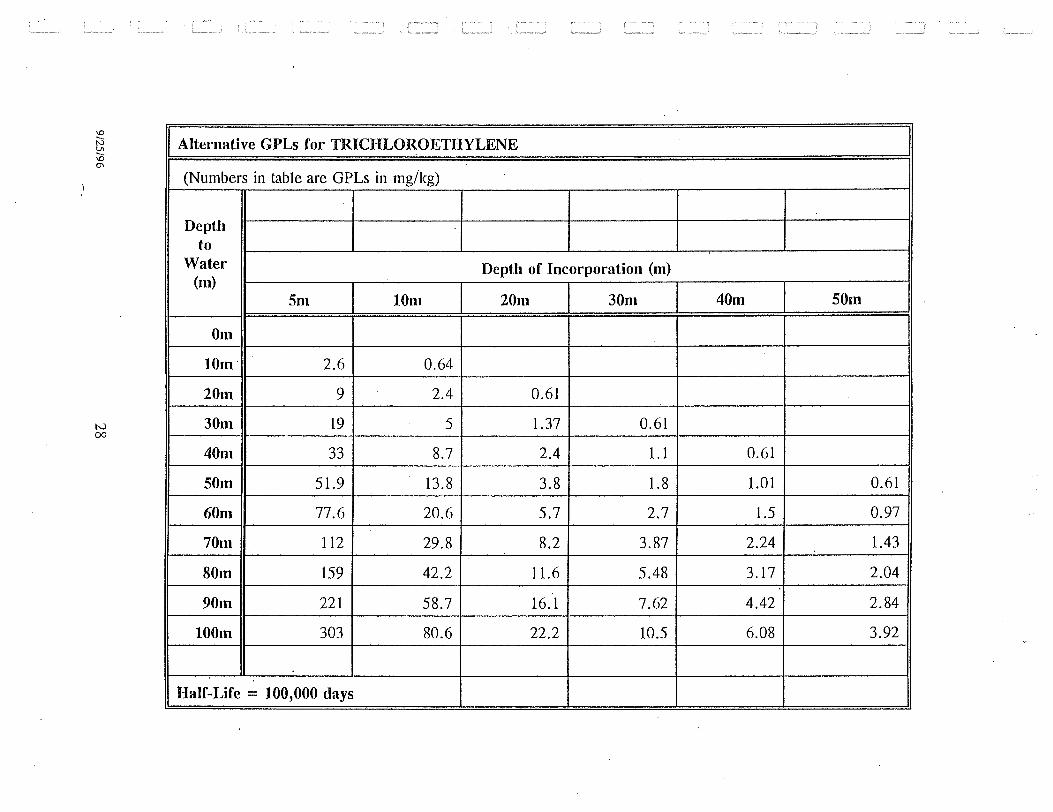
Alternative GPLs for TRICHLOROETHYLENE

(Numbers in table are GPLs in mg/Icg)

Depth t.o

Water Dept.h of Incorporation (m) (m)

5m 10m 20m 30m

Om

10m· 2.6 0.64

20m 9 2.4 0.61

30m 19 5 1.37 0.61

40m 33 8.7 2.4 1.1

50m 51.9 13.8 3.8 1.8

60m 77.6 20.6 5.7 2.7

70m 112 29.8 8.2 3.87

80m 159 42.2 11.6 5.48

90m 221 58.7 16.1 7.62

lOOm 303 80.6 22.2 10.5

Half-Life == 100,000 days

40m 50m

0.61

1.01 0.61

1.5 0.97

2.24 1.43

3.17 2.04

4.42 2.84

6.08 3.92

tv \0

4E+2

a H

':.( 2E+2

~ w ~ 0 (_)

:J '\. IJ)

::J

z 0 H

0E+0

4E+2

':.;: 2E+2 (k:

~ w (_) z 0 (_)

0E+0

0

0



++-+*+WTFUT fRCtl VADOSE-Zct£ I"KlDEL - Fl..!'K:TION 11'1'\.JT TO SATLRATED MOOEL

( V-Z Ol) A S-Z Dll- • ••••

100000 200000 301211211210 TIME ( DAYSl

LIQUID-PHASE CONCENTRATION VS TIME FOR VADOSE-ZONE AND SATURAT~ZONE MODELS

--- VADOSE ZONE SA Tl.RA TED :ZCX'£

' I I I I \

' \ ' ' ' ' ' ~

100000 200000 ::300000 400000 TIME <DAYS)

SITE NAME/ ID --------------TRICHLOROETHYLENE

KOC = . 1260E+ 03 cm3/o

KH = .3000E+00 HALF-LIFE C IN VADOSE ZONE) = .10E+06 doys HALF-LIFE (IN SATURATED ZONE) = . I0E+06 doyo GROUNDWATER STANDARD= 6.0000 ug/L SOIL HEALTH-BASED GUIDANCE LEVEL= 120.00 mg/kg

DEPTH TO GROUNDWATER= 20.0 m AQUIFER MIXING-CELL FACTOR= 1.0 DISTANCE TO COMPLIANCE P9INT = 30.6 m BULK DENSITY= 1.60 g/cm POROSITY = . 26 SOIL FOC= . 0010 AQUIFER FOC = .0010 SOIL MOISTURE CONTENT .16 MOISTURE FLUX THROUGH WASTE CELL= .70E-02 cm/d"'y MOISTURE FLUX OUTSIDE WASTE CELL= .70E-02 om/doy GROUNDWATER VELOCITY = 10.00 om/doy DIFFUSION LAYER THICKNESS .60 om DEPTH OF INCORPORATION = 10.000 m RELEASE WIDTH 10.0 m

2 AIR DIFFUSION COEF. = .7000E+04 om /9oy WATER DIFFUSION COEF. = .7000E+00 om /doy INITIAL CONTAMINANT CONCENTRATION IN SOIL = ug/om 3

VADOSE-ZONE TIME TO PEAK= .1250E+05 DAYS VADOSE-ZONE PEAK CONCENTRATION~ .3762E+03 ug/L SATURATED-ZONE TIME TO PEAK .I308E+05 DAYS SATURATED-ZONE PEAK CONCENTRATION = .9361E+02 ug/L CELL THICKNESS AT COMPLIANCE POINT 11.2 em CELL GPL = .3237E-01 mg/tg

GPL = .2370E+01 mg/kg (odjuatsd ior .820E+01m psrioroted tntervol)

1000

,...-.,

Ol 100 .:::£ ...._ Ol E --..---' Q.. (9 10

1

Alternative GPLs for Tetrachloroethylene ~

-f'"Y I I I_ 'I I l ~ I I ~!!ill

I I ~)~ I -----~ m- 1

: ~Y: I j.---f~ ~-I I I I

~

~ .-!if

'"''-v/ ~ ,..J---"'

/ mm~ s:r-__i/ I _j~ I I ...-r-- ..---r--

I I _,..1.\flll I I ~ I _.-- I .-i~

I l

I

: I

··- l l

0

j/ !'!!!!!

I / )\

/ /.

' ~ (I v

I

10 20

~~ I ~~j_-v~ I ~< ---+-C ~ J--~ ~ ~ I :___.( I I

/ - ,_ ,....,,/ / v ..,,.,._,....,

'i:Y I /,/ ~ --"'1-" ~/ 1/):J' I ~y I /~ ~- I

~v: vr ~~~~ I

I

30 40 50 60 70 Depth to Groundwater (m)

- I I

l : : : : I

' I

80 90 100

-o- 5m ·--~·--- 1 011! --\1-- 20m --®- 30m -----6:- 40m -~- 50m

Alternative GPLs for TETRACHLOROETHYLENE


Depth to

Water Depth of Incorporation (in) (m)

Sm 10m 20m 30m 40m 50m

Om

10m 5.6 1.3

20m 21.5 5.5 1.3

30m 49 12.7 3.2 1.3

40m 93.4 24 6.2 2.7 1.3

50m 161 41.4 11 4.7 2.5 1.3

60m 263 67.7 17.5 7.7 4.2 2.4

70m 415 107. 27.6 12.2 6.6 4

80m 638 164 42.4 18.9 10.3 6.2

90m 966 249 64.2 28.6 15.6 9.4

lOOm 1444 372 95.9 43 23.3 14.1

Half-Life = 100,000 days

z 0 H

2E+2

~ 1E+2 tY

~ ~ 8

2E+2


LIQUID-PHASE CONCENTRATION VS TIME (CORRECTED TO INITIAL ER£AKTI-RCU3H)

0

*"'**>~<OUTPUT FRCtl VAOOSE-ZO'£ liXJEL - FI..W'lCTION II\FUT TO SATLRATED MOOEL

<V-Z Dtl/(9-Z Dtl- •••••

100000 200000 300000 TIME (DAYS)


' I\ I I I I I 1 I 1 I I I I I I I I I I I I I I I I I I I I I \ I \ I '

-- - VADOSE ZO'£ - SATI..R<ATED ZONE

'

100000 200000 300000 TIME (DAYS)

SITE NAME / ID ------------------------------TETRACHLOROETHYLENE

KOC = .3640E+03 cm3/a

KH = .5450E+00 HALF-LIFE (IN VADOSE ZONE) = .10E+06 doy~ HALF-LIFE (IN SATURATED ZONE) = .10E+06 doyc GROUNDWATER STANDARD = 6.0000 ug/L SOIL HEALTH-BASED GUIDANCE LEVEL = 64.00 mg/kg

DEPTH TO GROUNDWATER = 20.0 m AQUIFER MIXING-CELL FACTOR~ 1.0 DISTANCE TO COMPLIANCE P9INT 30.6 m BULK DENSITY= 1.60 g/cm POROSITY . 25 SOIL FOC= .012110 AQUIFER FOC ~ .0010 SOIL MOISTURE CONTENT = . 16 MOISTURE FLUX THROUGH WASTE CELL= .70E-02 cm/doy MOISTURE FLUX OUTSIDE WASTE CELL= .70E-02 om/doy GROUNDWATER VELOCITY = 10.00 om/day DIFFUSION LAYER THICKNESS = .60 om DEPTH OF INCORPORATION = 10.000 m RELEASE WIDTH = 10.0 m

2 AIR DIFFUSION COEF. = .7000E~04 om /goy WATER DIFFUSION COEF. = .7000E~00 om /day INITIAL CONTAMINANT CONCENTRATION IN SOIL 1 ug/om 3

VADOSE-ZONE TIME TO PEAK= .1430E+06 DAYS VADOSE-ZONE PEAK CONCENTRATION= .. 1630E+03 ug/L SATURATED-ZONE TINE TO PEAK= .1522E+05 DAYS SATURATED-ZONE PEAK CONCENTRATION= .4046E+02 ug/L CELL THICKNESS AT COMPLIANCE POINT 11.2 om CELL GPL = .7490E-01 mg/kg

GPL a .5484E+01 mg/kg (ad juG ted ior .820E+01m poriora Led ln terva I)

IV. SCREENING APPROACH FOR INORGANIC CONTAMINANTS

Screening levels were developed for metals with A WQS using a simplified approach based on a mixing cell model and the ratio between the site-specific total and leachable metal concentrations. See Appendix C for a detailed explanation. This simplified approach was used because of the complex nature of modeling fate and transport of metals in the vadose zone. The input parameter values are the same as those used in the organic contaminant modeling. Calculations show that the Residential HBGL is sufficient to protectgroundwater quality for five metals (arsenic, barium, beryllium, chromium and ~thallium). The NonResidential HBGL for arsenic and beryllium is also protective of groundwater quality. For other metals, soil concentrations needed to protect groundwater quality were developed.

The screening approach for inorganics incorporates three steps and is similar to that for organic contaminants. Figure 1 is a t1ow diagram showing the steps in the screening process.

Step 1

The initial screening step determines whether the m~tal of concern at the site poses a threat to groundwater quality. Minimum GPLs are provided (Table 4) that represent soil contaminant concentrations protective of groundwater quality in a "worst-case" situation 'where all the metals in the soil leach completely to groundwater regardless of the depth to groundwater. If the Minimum GPL is less than the HBGL, the Minimum GPL may be used as the alternative soil cleanup standard if the party performing the remedial action chooses not to undertake further site characterization.

Step 2

If the Minimum GPL is less than the HBGL and the party chooses not to use the Minimum GPL as the soil cleanup standard, a second screening level is available. This step requires site-specific information on the relationship between the total metals concentration in the contaminated soil and the leachable fraction of that metal determined using either EPA Method 1311 Toxicity Characteristic Leaching Procedure (TCLP), EPA Method 1312 Synthetic Precipitation Leaching Procedure (SPLP) or an alternative approved leaching procedure appropriate for site conditions. If sufficient site-specific data have been collected to determine the ratio between the total metals concentration and leacpate concentration, an Alternative GPL may be calculated using the following equation:

X. = (292. 9)RCw

9/25/96 33

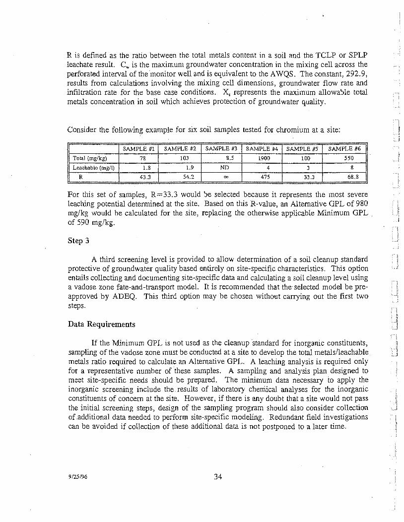
R is defined as the ratio between the total metals content in a soil and the TCLP or SPLP leachate result Cw is the maximum groundwater concentration in the mixing cell across the perforated interval of the monitor well and is equivalent to the AWQS. The constant, 292.9, results from calculations involving the mixing cell dimensions, groundwater flow rate and infiltration rate for the base case conditions. Xs represents the maximum allowable total metals concentration in soil which achieves protection of groundwater quality.

Consider the following example for six soil samples tested for chromium at a site:

SAMPLE #1 SAMPLE #2 SAMPLE #3 SAMPLE #4 SAMPLE #5 SAMPLE #6

Total {mg!kg) 78 103 8.5 1900 100 55o 11

Leachable {mg/1) 1.8 1.9 ND 4 3 8

R 43.3 54.2 co 475 33.3 68.8

For this set of samples, R=33.3 would be selected because it represents the most severe leaching potential determined at the site. Based on this R-value, an Alternative GPL of 980 mg/kg would be calculated for the site, replacing the otherwise applicable Minimum GPL . of 590 mg/kg.

Step 3

A third screening level is provided to allow determination of a soil cleanup standard protective of groundwater quality based entirely on site-specific characteristics. This option entails collecting and documenting site-specific data and calculating a soil cleanup level using a vadose zone fate-and-transport modeL It is recommended that the selected model be preapproved by ADEQ. This third option may be chosen without carrying out the first two steps.

Data Requirements

If the Minimum GPL is not used as the cleanup 'standard for inorganic constituents, sampling of the vadose zone must be conducted at a site to develop the total metals/leachable metals ratio required to calculate an Alternative GPL. A leaching analysis is required only for a representative number of these samples. A sampling and analysis plan designed to meet site-specific needs should be prepared. The minimum data necessary to apply the inorganic screening include the results of laboratory chemical analyses for the inorganic constituents of concern at the site. However, if there is any doubt that a site would not pass the initial screening steps, design of the sampling program should also consider collection of.additional data needed to perform site-specific modeling. Redundant field investigations can be avoided if collection of these additional data is not postponed to a later time.

9125196 34

Table 4. Minimum GPLs for Metals

Minimum GPL, Residential HBGL Non-Residential Metal x20 (mg/kg) (mg/kg) HBGL (mg/kg)

Antimony 35 47* 165* Arsenic 290 0.91 3.82 Barium 12,000 8200 28,700* Beryllium 23 0.32 1.34 Cadmium 29 58* 244* Chromium 590 580 2436* Lead 290 400* 1400* Mercury 12 35* 123* Nickel 590 2300* 8050* Selenium 290 580* 2030* Thallium 12 8.2 28.7*

* HBGL is not sufficiently low to prevent groundwater contamination

NOTE: Minimum GPLs have been rounded to two significant digits.

9/25/96 35

APPENDIX A

DESCRIPTION OF APPROACH FOR ORGANIC CONTA.J.VIINANTS

A-I. CONCEPTUAL MODEL FOR ORGANIC CONTAMINANTS

The conceptual model for transport of organic compounds in the vadose zone was developed to be as simple and straightforward as possible, without neglecting the important conditions and processes that affect transport of organic compounds through the vadose zone. A simple conceptual model can be applied to a large number of sites with different characteristics, whereas input data required for more complex vadose zone transport models can be difficult or expensive to attain and may not substantially increase the accuracy of the modeling results.

The conceptual model is based on hydrogeologic characteristics common to unconsolidated sediments in the alluvial basins of Arizona. The conceptual model, and therefore the screening levels developed via vadose zone transport modeling, may not be appropriate for sites where the vadose zone consists chiefly of consolidated rock. The conceptual model comprises two distinct units, the vadose zone and the saturated zone.

Screening levels for organic compounds in soil were developed based on modeling the transport of organic compounds through the vadose zone and saturated zone to a downgradient groundwater compliance point (groundwater monitoring well). Screening levels consist of concentrations of organic compounds detected in soil in the vadose zone that are projected to result in concentrations in groundwater at the compliance point equal to the A WQS for those compounds. Screening levels for organic compounds are variable, depending on mobility of the compound, depth of occurrence of the compound in the vadose zone, and the depth to groundwater below land surface.

A. Conceptual Model for the Vadose Zone

The conceptual model for the vadose zone is a single layer of unconsolidated, poorly sorted, basin-fill deposits consisting chiefly of sand and silt. Organic compounds are assumed to occur in the vadose zone from land surface to some depth. The chief processes assumed to affect transport of organic compounds in the vadose zone conceptual model are: 1) advection of organic compounds dissolved in recharge water, which moves downward through the vadose zone and eventually reaches the groundwater table (dissolved-phase advection); 2) diffusion of organic compounds in the vapor phase (vapor-phase diffusion); 3) adsorption of organic compounds to solid-phase organic carbon (solid-phase adsorption); and 4) degradation of organic compounds. The presence and movement of non-aqueous phase liquids (NAPLs) are not included in the conceptual model.

9/25/96 A-1

DISSOLVED-PHASE ADVECTION: One of the important processes for downward transport of organic compounds in the vadose zone is dissolved-phase advection. Infiltration of precipitation at land surface results in a small amount of water moving downward through the vadose zone and eventually reaching the saturated zone. The rate of water movement in the vadose zone is very slow; recharge to the saturated zone from precipitation infiltrating at land surface may require many years. As the water slowly moves downward, organic compounds may evaporate out of this water phase or adsorb to the solid phase according to partitioning relationships between organic compound concentrations in the dissolved phase, the vapor phase, and the solid phase. Because water movement in the vadose zone is slow, the partitioning relationships are assumed to be equilibrium relationships. These equilibrium relationships are incorporated into the conceptual model.

VAPOR-PHASE DIFFUSION: Another important process for transport of organic contaminants, particularly volatile organic compounds (VOCs), in the vadose zone is vaporphase diffusion. VOCs diffuse in the vapor phase in all directions from zones of higher VOC concentrations to zones of lower VOC concentrations. For simplification, the conceptual model is limited to one dimension and, therefore, only considers movement upward and downward. Unlike diffusion of solutes in groundwater, vapor-phase diffusion of VOCs can be relatively rapid. Because concentrations of VOCs in the atmosphere above land surface are essentially maintained at zero, the atmosphere functions as an "infinite sink" for VOCs and provides a constant upward gradient for vapor-phase diffusion.

SOLID-PHASE ADSORPTION: The mobility of solutes in the vadose zone is affected by solid-phase adsorption. Because adsorption of organic compounds from the dissolved phase to the solid phase is generally considered to occur chiefly to the organic carbon fraction of the solid phase sediments, the conceptual model only considers the fraction of organic carbon for solid-phase adsorption. The Freundlich sorption model, with a linear adsorption isotherm for partitioning of dissolved-phase organic compounds to solidphase organic carbon, is appropriate for the hydrogeologic conditions and organic compounds considered in the conceptual model.

DEGRADATION: Many organic compounds undergo some degree of degradation, usually biodegradation, in the vadose zone. Degradation reactions may transform toxic organic compounds into non-toxic components or other toxic compounds. Rates of biodegradation of organic compounds in the vadose zone are described using first-order decay equations and appropriate degradation half-lives for the modeled compounds.

B. Conceptual Model for the Saturated Zone

The conceptual model for the saturated zone is a single aquifer or aquifer zone dominated by horizontal flow, with a groundwater compliance point located 100 feet downgradient from the source of organic compounds in the vadose zone. Organic

9/25/96 A-2

compounds are assumed to enter the saturated zone solely from the vadose zone. The principal process assumed to affect transport of organic compounds in the saturated zone is advective-dispersive transport. A typical application for groundwater flow modeling may include advective-dispersive transport and diffusive transport of dissolved constituents. However, due to the short distance between the point of entry of organic compounds to the saturated zone and the groundwater compliance point, the simulation of solute transport in groundwater can be simplified. Therefore, the conceptual model for transport processes in groundwater comprises a mixing zone in which organic compounds reaching the groundwater table from the vadose zone mix instantaneously with the groundwater.

A-II. MODEL SELECTION

After an initial screening of available models, the Working Group further evaluated three vadose zone transport modeling programs for potential use in developing the proposed screening levels: SESOIL, VLEACH, and the ADEQ model, which is a computer code based on Dr. William Jury's well-documented and accepted Behavior· Assessment Model. All of these models simulate the principal organic chemical transport processes that occur in the vadose zone. The principal conclusions from comparison of the models are summarized as follows:

1.

2.

9/25/96

SESOIL has been used as a screening tool by several other states, including California, Wisconsin, and Massachusetts. SESOIL and VLEACH have been extensively reviewed and approved for use at several hazardous waste sites to evaluate threats to groundwater of vadose zone contaminants. The ADEQ model was recently developed by ADEQ and has not been as extensively tested or reviewed, but the ADEQ model is based on the reviewed and tested theories and methods developed by Dr. Jury, who is widely recognized as an expert in vadose zone transport processes and modeling.

The "state-of-the-art" in vadose zone transport modeling is not as well developed as for groundwater modeling, and the flow and transport processes for the vadose zone are more difficult to measure and to simulate than for groundwater. SESOIL is the most complex of the three models and is more versatile than VLEACH or the ADEQ model, but requires more site-specific input parameters and assumptions about vadose zone conditions. Because vadose zone conditions vary substantially from site to site and because site conditions are not likely to be characterized completely, results from a relatively complex model, such as SESOIL, may not be more accurate or representative of actual transport processes than results from a simpler model. Therefore, a simple vadose zone transport model may be as suitable or more suitable than a complex model for the screening process.

A-3

3. The ADEQ model includes a groundwater model and was developed specifically to compute concentrations for organic compounds in soil based on simulated concentrations of organic compounds in groundwater. The ADEQ model calculates a groundwater protection level (GPL) that is the maximum soil concentration that will not cause an A WQS to be exceeded at a specified point of compliance in the aquifer. SESOIL and VLEACH are vadose zone transport models that do not include groundwater models .. Numerous trialand-error model runs must be conducted using SESOIL or VLEACH to develop a single vadose zone screening level. Therefore, the ADEQ model is much easier and faster to use for the development of vadose zone screening levels.

Based on the suitability of the ADEQ model for simulating the critical vadose zone and groundwater transport processes and based on the ease of use, the Leachability Working Group selected the ADEQ model to develop vadose zone screening levels for organic compounds. The ADEQ model, which was first developed in June 1993 and has been modified only slightly since then, is available at no charge from ADEQ; no license is required to use or copy the ADEQ model. However, the ADEQ model incorporates links to a commercial program, GRAPHER, into the code. Therefore, ownership of a licensed copy of GRAPHER is a prerequisite to possession or use of the ADEQ model.

A-ill. ASSIGNMENT OF MODEL INPUT PARAMETER VALUES

The model input parameters were selected to be reasonable and without bias regarding effects on resulting screening levels. The Wor.king Group agreed that using conservative values for every input parameter would be inappropriate because effects of multiple biased input parameters tend to be multiplicative and would result in projected screening levels several orders of magnitude smaller than necessary to protect groundwater resources. Three general categories of model input parameters are required for the ADEQ model: 1) vadose zone input parameters; 2) groundwater input parameters; and 3) chemical input parameters.

A. Vadose Zone Input Parameters

DEPTH TO GROUNDWATER AND DEPTH OF INCORPORATION: The relationship between depth to groundwater and depth of- incorporation (maximum depth where concentrations of organic compounds meet or exceed Minimum GPLs in the vadose zone) was found to be a critical site-specific variable. Therefore, for each organic compound, graphs of screening levels were developed based on the input of several values to the ADEQ model for depth to groundwater and depth of contaminant incorporation.

9/25/96 A-4

i '

These graphs provide a method for determining "site-specific" screening levels based on the actual depth of occurrence of organic compounds and depth to groundwater at a site. Only these two vadose zone parameters were varied during modeling to develop the screening levels. .

RELEASE WIDTH: The release width is the horizontal dimension of the contaminated zone parallel to the direction of groundwater movement. The value for release width input to the model was 10 meters (33 feet). This width is considered to be typical of most accidental releases of organic compounds (underground storage tank leaks, for example).

BULK DENSITY OF SOIL: The value input to the model for dry bulk soil density was 1.5 grams per cubic centimeter (g/cm3

). Bulk densities for basin-fill deposits typically are in the range from 1.3 to 1.8 g/cm3

• Therefore, 1.5 g/cm3 is considered to be a reasonable value for model soil bulk density.

POROSITY OF SOIL: Porosity is used in model calculations for: (1) average interstitial groundwater velocity in the saturated zone; (2) contaminant mass partitioning to the vapor and dissolved phases in the vadose zone; and (3) vapor-phase diffusive flux in the vadose zone. A single porosity value is input to the model; no distinction is made in the model between total porosity and effective porosity. The value input to the model for soil porosity was 25 percent. Porosities for basin-fill deposits typically are in the range from 20 to 35 percent. Therefore, 25 percent is considered to be a reasonable value for model soil porosity.

FRACTION OF ORGAN1C CARBON IN SOIL: The value input to the model for fraction of organic carbon in soil was 0.001 (0.1 percent). Organic carbon fractions in basin-fill deposits are very small and typically are in the range from 0.0005 to 0.005. Therefore, 0.001 is considered to be a reasonable value for model fraction of organic carbon.

VOLUMETRIC MOISTURE CONTENT: The value input to the model for volumetric moisture content of soil was 15 percent. Volumetric moisture contents in basinfill deposits typically are in the range from 5 to 25 percent. Therefore, 15 percent is considered to be a reasonable value for model soil moisture content.

RECHARGE RATE: This parameter is variable and difficult to measure; therefore, a conservative recharge rate was intentionally selected to yield conservative soil screening levels. The model requires input of two infiltration rates--one for the contaminated area and one for the area between the contaminated area and the downgradient compliance point. . However, a single value of 0.007 em/day (1 inch per year) was input to the model for both recharge variables. Diffuse recharge rates for desert alluvial basins of the Southwest are believed to be less than about 0.0035 em/day (0.5 in/yr). Rates of recharge at mountain fronts and in stream channels likely are generally larger than diffuse recharge rates. The

9/25/96 A-5

model's recharge rate of 0.007 em/day is larger than most estimates of recharge rate for desert alluvial basins.

DIFFUSION LAYER THICKNESS: The model simulates mass transfer from the gas phase in the vadose zone to the atmosphere using a diffusion layer. The value input to the model for diffusion layer thickness was 0.5 em (0.2 in). The Working Group adopted the same numerical value used by Jury in his Behavior Assessment Model.

B. Groundwater Input Parameters

DISTANCE TO MONITOR WELL (GROUNDWATER COMPLIANCE POINT): The horizontal distance from the point of vadose zone contamination to the downgradient groundwater compliance point input to the model was set at 30.5 meters (100 feet). This distance is consistent with a variety of setbacks established in environmental regulations (such as the distance a septic tank must be set back from a domestic well), and likely is as close to a waste site as a drinking-water well would be constructed.

AQUIFER MIXING CELL FACTOR: Aqueous dispersion of organic compounds in groundwater is crudely simulated in the model by an aquifer mixing cell factor. This factor increases the vertical thickness of successive mixing cells used by the model to simulate transport of organic compounds in the aquifer. The aquifer mixing cell factor input to the model was 1.0; therefore, each mixing cell increases in thickness equivalent to the amount of recharge impinging on the mixing cell during each time step. Further discussion of the aquifer mixing cell factor is presented in Appendix B. It should be noted that due to the small recharge rate and the relatively large monitor well perforated interval input to the ADEQ model, only an unreasonably large increase in the aquifer mixing cell factor affects model results.

FRACTION OF ORGANIC CARBON IN THE AQUIFER: The value input to the model for fraction of organic carbon in the aquifer was 0.001 (0.1 percent). Organic carbon fractions in Arizona's basin-flll deposits are very small and typically are in the range from 0.0005 to 0.005. Therefore, 0.001 is considered to be a reasonable value for model fraction of organic carbon.

AVERAGE LINEAR GROUNDWATER VELOCITY: The average linear velocity-not Darcian velocity or specific discharge--input to the model was 10 em/day (120 ft/yr). Groundwater velocities in aquifers- in Arizona's basin-fill deposits range widely, but are commonly in the range from about 1 to 100 em/day. Therefore, 10 em/day is considered to be a reasonable order-of-magnitude value for groundwater velocity. ·

PERFORATED INTERVAL OF MONITOR WELL: The perforated interval of the downgradient groundwater monitor well (compliance point) input to the model was set at 8.2

9/25/96 A-6

meters (27 feet). A perforated interval of 5 to 10 meters (15 to 30 feet) is typical for groundwater monitor wells in Arizona's basin-fill aquifers. Therefore, 8.2 meters is believed to be a reasonable value for the perforated interval of the downgradient groundwater monitor well. The perforated interval is directly proportional to resultant screening levels; for example, if the perforated interval input to the model were doubled to 16.4 meters (54 feet), all soil screening levels also would double.

GROUNDWATER STANDARD: The model requires input of the groundwater standard that must be achieved at the compliance point. The model uses the AWQSs, which are identical to EPA MCLs for drinking water. The model calculates maximum soil concentrations of organic compounds that will result in groundwater concentrations equal to the groundwater standards.

SOIL HEALTH-BASED GUIDANCE LEVEL lliBGL): This parameter is input solely for reference purposes, to compare the HBGL with the screening level projected by the model. This parameter is not used in any model calculations.

C. Chemical Input Parameters

The ADEQ model requires the input of several parameters for each organic compound modeled. Chemical-specific values for these parameters are available in standard reference literature; values from reference literature were input to the model for organiccarbon partitioning coefficient (K0 c) and Henry's constant (K~, and are summarized later in this report.

Values for aqueous diffusion coefficient and free-air diffusion coefficient in water also are required. For the compounds modeled, the variation in these values is small and has little effect on model results. Therefore, a single value for each of these parameters was input to the ADEQ model for all of the organic compounds modeled.

AQUEOUS DIFFUSION COEFFICIENT: The model input value for aqueous diffusion coefficient for organic compounds was 0.7 cm2/day. Reported values for aqueous diffusion coefficient for most of the organic compounds modeled are in the range from about 0.6 to 0.9 cm2/day. It should be noted that the ADEQ model is nearly insensitive to the value input for aqueous diffusion coefficient.

FREE-AIR DIFFUSION COEFFICIENT: The model input value for free-air diffusion coefficient for organic compounds was 7,000 cm2

/ day. Reported values for free-air diffusion coefficient for most of the organic compounds modeled are in the range from about 6,000 to 9,000 cm2/day.

9/25/96 A-7

DEGRADATION HALF-LIFE: The model input value for the degrad(l.tion half-life for benzene, toluene, ethylbenzene, and xylene (BTEX compounds) was 1,000 days (2.7 years). These compounds are present in fuels and, therefore, are among the most common organic compounds released in the vadose zone. The model input value for degradation halflife for the other organic compounds, most of which are chlorinated, was 100,000 days (270 years). Reported degradation half-lives for BTEX compounds in laboratory studies are generally less than 1,000 days, and reported degradation half-lives for the other organic compounds range from 100 to over 10,000 days. It should be noted that degradation halflives vary substantially, are highly dependent on local site conditions, and are difficult to determine in the field. In addition, many chlorinated organic compounds are very persistent or degrade to other toxic compounds. Therefore, a 1 ,000-day degradation half-life for BTEX compounds and a 100,000-day degradation half-life for the other organic compounds modeled are considered to be conservative input values for the model. The degradation halflife is the most sensitive factor in affecting the model results.

9/25/96 A-8

Table A-1. Sorption and Volatilization Constants Used in Developing GPLs

Soil Organic Dimensionless Carbon Partition Henry's Law Coefficient, Koc Constant, KH

Benzene 64.5 0.221

Carbon Tetrachloride 439 0.96

o-Dichlorobenzene 186 0.050

para-Dichlorobenzene 158 0.13

1 ,2 Dichloroethane 14 0.038

1,1 Dichloroethylene 65 0.87

cis-1 ,2-Dichloroethylene 49 0.12

trans-1 ,2-Dichloroethylene 59 0.22

1 ,2-Dichloropropane 27 0.096

Ethylbenzene 95 0.27

Monochlorobenzene 330 0.15

Styrene 741 0.019

Tetrachloroethylene (PCE) 364 0.545

Toluene 257 0.269

Trihalomethanes (Total) 44 O.i2

1,1, 1,-Trichloroethane (TCA) 152 0.56

Trichloroethylene (TCE) 126 0.3

Xylenes (Total) 129 0.256

Alachlor 101.7 8.31xlo-7

Atrazine 38.5 1.03xlo-7

Carbofuran 95.4 4.4xlo-s

1 ,2-Dibromo-3-chloropropane (DBCP) 126 0.0104

Ethylene dibromide (EDB) 44 0.104

9/25/96 A-9

Endrin 34,000 3.13x10-4

Lindane 1388 7.52xl0·5

2,4-Dichlorophenoxyacetic acid (2,4-D) 30.5 0.811

Trichlorophenoxypropionic acid (2,4,5-TP or 2600 5.45xl0·7

Silvex)

Bolded data were supplied to ADEQ by pesticide manufacturers. All other Kuc and Kn values are from general groundwater chemical references. ·

9/25/96 A-10

A-IV. MODEL REVIE\V AI\TD VERIFICATION

The ADEQ model code was peer reviewed by Dr. William A. Jury. In addition, the results of ADEQ model simulations were compared to Jury's Behavior Assessment Model results. The comparison indicated that the model yielded identical results to the Behavior Assessment Model under the selected conditions.

The Leachability Working Group conducted verification simulations to compare soil screening levels projected by the ADEQ model for eight VOCs to soil screening levels developed by the Massachusetts Department of Environmental Protection (MDEP) using SESOIL and AT123D (a simple groundwater transport model). Results oftheMDEP's work are presented in 11BACKGROUND DOCUMENTATION FOR THE DEVELOPMENT OF THE MCP NUMERICAL STANDARDS, 11 published by the MDEP in April1994. Where possible, input parameters similar to those used by MDEP were input into the ADEQ model, although the modeling procedures and input requirements for SESOIL are substantially different from those required for the ADEQ model. Despite the different formats used by SESOIL and the ADEQ model, soil screening levels projected by the two models are similar. The VOCs compared and the screening levels projected by each model are summarized as follows:

COMPOUND Benzene Ethylbenzene Toluene o-Xylene Trichloroethene (TCE) Tetrachloroethene (PCE) Trichloroethane (TCA) Naphthalene

PROJECTED SCREENING LEVEL (microe:rams per kilogram)

SESOIL ADEQ MODEL 280 222

84,800 70,600 80,600 88,000

833,300 781' 100 380 318 430 290

33,800 30,100 62,200 32,300

In summary, results of review and verification of the ADEQ model indicate that it adequately simulates the chief vadose zone transport processes and it produces results comparable to those generated by a widely-accepted model (BAM) and an EPA-approved model (SESOIL). Therefore, the ADEQ model is acceptable for the purpose of developing screening levels for organic compounds in the vadose zone.

9/25/96 A-ll

A-V. SENSITIVITY ANALYSIS

A sensitivity analysis was conducted in order to evaluate the effect of changes in several key input parameters on the model projections. The sensitivity analysis consisted of a series of model simulations in which the selected parameter was varied over a reasonable range while all. other parameters remained constant. Input parameters included in this sensitivity analysis were contaminant half life, depth to groundwater, soil· bulk density/porosity, recharge rate, release width, soil moisture content, fraction organic carbon, and air diffusion layer thickness.

Some of the sensitivity analysis simulations were carried out during the process of evaluating the model, prior to the selection of the fmal"base-case" parameter estimates. As a result, some of the sensitivity analysis simulations were run with slightly different sets of "base-case" parameters. Because the focus of the sensitivity analysis was to determine the change in model projections associated with a change in an individual parameter, it was not necessary that all sensitivity analysis simulations include the same set of base-case parameters.

A summary of the sensitivity analysis is presented in Table 2. The last column in Table 2 presents the ratio of the change in model results to the change in input parameter value. This ratio, which we have referred to as the Sensitivity Quotient, provides a general measure of the relative model sensitivity to different parameters. The higher the ratio, the more sensitive the parameter. Based on this analysis, the model is most sensitive to the halflife of the contaminant and the depth to groundwater. The model is less sensitive to changes in bulk density/porosity, recharge rate, initial water content and fraction of organic carbon. The model is insensitive to changes in the air diffusion layer thickness. The following sections provide additional observations regarding the sensitivity of the model to selected parameters.

A. Half-Life

The model provides for first-order degradation of contaminants. The degradation rate is input in the form of a half-life. For the sensitivity analysis, the half-life was varied from 1,000 days to 100,000 days. The value of 100,000 days was sufficiently long to minimize the effect of degradation on the model results. There is no provision in the model code for disabling the contaminant degradation; however, assigning a half-life that is much longer than the time simulated has the effect of making degradation negligible.

The results of this analysis showed that the effects of degradation are most pronounced for simulations with a shallow depth of incorporation and a large depth to groundwater. The half-life data presented in Table 2 represent a 20 meter depth of

9/25/96 A-12

incorporation and a 50 meter depth to groundwater. The effect of a change in half-life was much less pronounced when the depth of incorporation was assumed to be the same as the depth to groundwater. This is due to the fact that degradation is a time-dependent process, so that when contaminants migrate a large distance to groundwater, there is sufficient time for degradation to be effective in removing contaminant mass from the system.

B. Depth to Groundwater

The model requires input for the depth to groundwater and the depth of incorporation of the contaminants in the soil profile. For the worst-case analysis, the depth of incorporation equals the depth to groundwater. Varying the depth to groundwater from 20 meters to 100 meters while maintaining a depth of contaminant incorporation of 20 meters, resulted in a 25-fold increase in the GPL due mainly to dispersion and adsorption of the contaminant into the uncontaminated portion of the vadose zone between the contaminated zone and the underlying groundwater table. The sensitivity analysis for this parameter used a 100,000 day half-life to minimize the concurrent effect that degradation would have on the model results.

The model results were sensitive only. to the difference between the depth of incorporation and depth to groundwater. For example, simulations with a 20 meter depth of incorporation and 40 meter depth to groundwater produced the same results as simulations with a 40 meter depth of incorporation and 60 meter depth to groundwater.

The depth of contaminant incorporation and depth to groundwater are key site-specific parameters that are relatively easy to measure and have a significant effect on model results. Unless it is assumed that contaminants extend from the surface to the groundwater table, site-specific data should be used for depth of incorporation and depth to groundwater.

C. Bulk Densitv and Porositv

Bulk density and porosity are related parameters. Soils with higher porosity contain more air spaces and therefore have lower bulk density. The average grain density in most soils is approximately 2.65. Based on this correlation, the bulk density and porosity were varied jointly in the sensitivity analysis. For the base-case scenario, the bulk density was assumed to be 1.5 g/cm3 and the porosity was assumed to be 25%. In the sensitivity analysis runs, the bulk density ranged 1.5 to 2.25 g/cm3 and porosity concurrently ranged from 43% to 15%. This is considered to be approximately the maximum reasonable range for soils in the desert basins of Arizona. The parameter used for comparison in the sensitivity analysis was the ratio of bulk density to porosity (Table 2).

9/25/96 A-13

The model results were only moderately sensitive to changes in bulk density and porosity. For simulations where the contaminant was assumed to extend all the way to the groundwater table, the Sensitivity Quotient was approximately 2. For simulations where there were 30 meters of clean soil between the bottom of the contaminated zone and the groundwater table, the Sensitivity Quotient was approximately 3.

D. Recharge Rate

In the base-case scenario, the recharge rate was estimated at one inch per year, which is considered to be representative of the maximum value for the desert basins of Arizona. The recharge rate affects the velocity of the contaminant migration through the vadose zone, and to a lesser extent the dilution of the contaminant in the saturated zone. Increasing the recharge rate results in more rapid transport of contaminants to groundwater. Changes in recharge have a nearly linear affect on the model results. For the sensitivity analysis, a 60-fold increase in the recharge rate resulted in a 63-fold decrease in the GPL.

E. Release Width

The release width is the distance over which contaminants are present parallel to the principal direction of groundwater flow. A longer release width indicates a larger contaminated area and consequently more mass of a contaminant reaching groundwater. The release width was set at 10 meters (approximately 33 feet) for the base-case simulations, consistent with an "average" release width for smaller sites such as underground storage tanks.

In the sensitivity analysis, the release width was increased by a factor of four from 10 to 40 meters. This change resulted in a four-fold decrease in the projected GPL. These simulations were run with TCE as the contaminant. Simulations with a more-degradable compound such as benzene may not result in a direct one-to-one relationship due to degradation of the contaminant in the longer groundwater flow paths.

F. Volumetric Water Content

The volumetric water content is the fraction of the soil volume that is occupied by water~ This parameter is held constant throughout the simulation and primarily affects the velocity of water flow through the vadose zone. A higher moisture content results in a lower velocity of water flow through the unsaturated zone, and also affects the partitioning of volatile contaminants between the liquid and vapor phases. In the sensitivity analysis, the

9/25/96 A-14

total porosity was assumed to be the highest reasonable value of 43%, the depth of incorporation was set at 20 meters and depth to groundwater was set at 30 meters. When the volumetric water content was varied from 0.001 to 0.43 (0.2% to 100% of the total porosity), the resultant GPL varied from 3.3 to 2.0. The maximum GPL occurred at a moisture content of 0.25 (58% of porosity) and the minimum GPL occurred at a moisture content of 0.41 (95% of the porosity).

In running the model, the GPL flrst increases with increasing initial moisture content and then decreases when the moisture content increases beyond 0.41. The initial moisture content was the only parameter evaluated in the sensitivity analysis that produced a nonmonotonic response in model results.

Moisture content varies according to soil type and availability of recharge. The model assumes a constant, uniform value for moisture content over the entire soil profile and throughout the entire simulation time. The moisture content should not be changed from the base-case value unless it can be shown from site-specific data that a different moisture content is appropriate for the entire soil profile.

G. Fraction of Organic Carbon

The fraction of organic carbon (FOC) in the soil determines the amount of an organic contaminant that will adsorb onto the soil. For the base-case scenario, the FOC was assumed to be 0.1 %, which is considered a reasonable value for desert soils. Increasing the FOC results in slower contaminant transport and a higher GPL. In the sensitivity analysis, the FOC was varied from 0.1% to 1%. Increasing the FOC by a factor of 10 resulted in an 8. 8 fold increase in the projected GPL.

H. Diffusion Laver Thickness

The diffusion layer thickness is the thickness of the layer of air above the soil surface in which the contaminant is assumed to be present. This parameter was included in Dr. Jury's original Behavior Assessment Model which was developed to assess the behavior of pesticides applied at shallow depths to crops. Decreasing the diffusion layer thickness results in a steeper concentration gradient at the soil surface and an increase in the loss of contaminants to the atmosphere.

In the base-case scenario, the diffusion layer thickness was set to 0.5 em which is the value suggested in the original Behavior Assessment Model documentation. In the sensitivity analysis, varying the diffusion layer thickness from 0.5 em to 5 ern had no significant effect on the projected GPL. The contaminant properties used in this analysis were those of vinyl

9/25/96 A-15

chloride, which is one of the most volatile of the common organic contaminants and sliould therefore diffuse most rapidly to the atmosphere. The insensitivity of the model is probably due to the relatively large depth of incorporation and the relatively high infiltration rate used in these simulations. The results indicate that the mass of contaminants diffusing upwards is insignificant compared to the mass migrating downwards.

A-VI. SENSITIVITY ANALYSIS CONCLUSIONS

The sensitivity analysis was conducted over reasonable assumed ranges of values for important, site-specific input parameters. Of the parameters evaluated, the model was most sensitive to the half-life of the contaminant and the depth to groundwater. The model was moderately sensitive to bulk density/porosity, recharge rate, release width, volumetric water content and fraction of organic carbon. The model was insensitive to the diffusion layer thickness.

For the purposes of site screening, a base-case scenario has been developed that incorporates a set of parameter values considered to be conservative but reasonable. The base-case scenario is not considered to be a worst-case scenario. Site-specific data may support adjustments to any of the base-case parameters, but any adjustment of the moresensitive input parameters based on site-specific data should require adjustment of all the other more-sensitive input parameters based on site-specific data as well.

9/25/96 A-16

Table A-2. Results of Sensitivity Analysis

PARAMETER INPUT MODEL OUTPUT SENSITIVITY PARAMETER RANGE RANGE (ADJ. GPL) QUOTIENT1

Half-Life 1,000 to 100,000 days 197,700 to 8.7 2.27 mg/kg

Depth to Groundwater 20 to 100 meters 0.43 to 5.0 10.8 mg/kg

Bulk Density/Porosity 0.28 to 0.06 1.31 to 1.9 0.17 mg/kg

Recharge Rate 0.1 to 6 in/yr 12.96 to 1.1 0.2 mg/kg

Release Width 10 to 40 meters 1.4 to 0.97 0.34 mg/kg

Volumetric Moisture 58 to 100 percent 3.47 to 0.94 Content porosity 2.03 mg/kg

Fraction Organic 0.1 to 0.01 percent 69.0 to 0.88 Carbon 609 mg/kg

Diffusion Layer Thick- 0.5 to 5.0 em 4.9 mg/kg 0.0 ness

1Calculated as the ratio of PerCent Change in Output to Percent Change in Input.

9/25/96 A-17

APPENDIXB

ADEQ MODEL

FOR DEVELOPING

GROUNDWATER PROTECTION LEVELS

TABLE OF CONTENTS

ACKNOWLEDGEMENT .

1

2

3

4

5

6

7

INTRODUCTION

A SYNOPSIS OF TRANSPORT AND FATE PROCESSES

RANGE OF MODELING OPTIONS

PROPOSED METHOD . . . . . 4.1 INTRODUCTION .... 4.2 MIXING CELL MODEL FOR THE SATURATED ZONE 4.3 BEHAVIOR ASSESSMENT MODEL FOR THE UNSATURATED ZONE 4.4 MODEL ASSUMPTIONS ... . 4.5 MODEL LIMITATIONS .... .

MODEL REVIEW AND VERIFICATION 5.1 VADOSE ZONE MODEL ..... . 5.2 MIXING CELL MODEL (SATURATED ZONE MODEL)

REFERENCES .

APPENDICES . . . . 7.1 PROGRAM OPERATION

ii

1

2

4

9 9 9

11 13 18

18 18 19

20

22 22

GPL -ii-

ACKNOWLEDGEMENT

The model described in this document is primarily the effort of Wyn Ross, Hydrologist, Arizona Department of Environmental Quality. Mr. Ross conceptualized, programmed and tested the model and drafted the essence of this report. His work was substantially completed in June 1993. Charles Graf, ADEQ Section Manager, guided the development of the model and reviewed the original report. Charles Hains, ADEQ Hydrologist, reviewed and tested the code, eliminated bugs that were identified, and revised the draft by Mr. Ross.

After the Leachability Working Group began evaluating the ADEQ model in 1995 for possible use in developing soil cleanup levels, Mr. Eric Zugay, Basin & Range Hydrogeologists, Inc., made many useful suggestions as part of his review of the model code and report. In 1996, Lyn Conner, working as a volunteer for ADEQ, improved file management aspects of the model and eliminated several bugs identified by the Leachability Working Group. Michele Robertson of ADEQ compiled all of the reviewer's comments and produ.ced this final version of the document.

The framework of the fate and transport model in the vadose zone is the Behavior Assessment Model developed by Dr. William A. Jury of the University of California at Riverside.

i ••• J

1 INTRODUCTION

ADEQ MODEL FOR DEVELOPING GROUNDWATER PROTECTION LEVELS

GPL -1-

In this document, the Arizona Department of Environmental Quality (ADEQ) outlines a methodology for estimating concentrations of crganic contaminants that can remain in soil yet be protective of groundwater quality. ADEQ has termed these concentrations "Groundwater Protection Levels" or 11GPLs." ADEQ's intent in developing this methodology was 'to answer the question: At what approximate concentration can an organic compound be left in soil such that an applicable Aquifer Water Quality Standard (AWQS) will not be exceeded at an appropriate compliance point within the aquifer underlying the contaminated soil? Because the methodology described in this document incorporates some of the basic chemical and hydrogeological principles that govern the transport of fluids and contaminants through the subsurface, the derived GPLs should prove useful in answering this question.

ADEQ completed the Fortran computer program in June 1993. This model processes the large amounts of numerical data that are generated while solving the contaminant fate and transport equations. The model simulates one-dimensional advective transport of organic compounds in the vadose zone and one-dimensional transport in the mixing cell flow domain of the saturated zone, allowing for adsorption, biodegradation, volatilization, and diffusion.

Since the model development, ADEQ has established soil cleanup standards in the Interim Soil Remediation Standards Rule which became effective March 29, 1996. For the interim rule, HealthBased Guidance Levels (HBGLs) for ingestion of soil were adopted as pre-determined risk-based cleanup standards. The rule also allows an alternative cleanup standard developed from a site-specif risk assessment. Either approach requires that, following remediation, remaining concentrations of contaminants in soil will not cause or threaten to cause groundwater contamination to exceed an AWQS at a point of compliance in the aquifer. The ADEQ model provides a method for calculating concentrations of organic contaminants in so - the GPLs - that will be protective of groundwater quality.

GPL -2-

2 A SYNOPSIS OF TRANSPORT AND FATE PROCESSES

The question of whether contaminant leaching from soil will cause a groundwater standard to be exceeded at some point (the compliance point) cannot be answered with certainty. In general, far too many unknowns exist regarding the hydraulic and retention properties of the medium, fate processes affecting the transformation of the contaminant, heterogeneity in the aquifer and vadose zone, and past and future conditions at the system boundaries for a complete and definitive analysis to be performed. However, as more resources are invested, more information about the system can be obtained to improve predictive capabilities. Therefore, any methodology developed to answer this question is necessarily a compromise between accuracy, simplicity, and cost.

Fate and transport processes significantly affect the dissolvedphase concentration at the compliance point. These processes depend on the properties of the chemical, the physical and biological characteristics of medium, and the environmental conditions that determine the state of soil moisture and soil air.

~ost contaminant movement in the soil occurs via the following mechanisms: mass flow of dissolved solute within moving soil water, diffusion and dispersion in the dissolved and vapor phases, convective flow of the vapor phase, and gravity-driven flow of nonaqueous phase liquid (NAPL). The relative importance of these mechanisms depends primarily on the volumetric air and water contents of the soil, the flux of moisture through the system, the phase partitioning of the chemical, and the nature of the contaminant release (e.g., NAPL vs. dissolved phase, constant-head pending vs. zero-head pending). The magnitude and temporal distribution of extrinsic events (e.g., irrigation or precipitation), together with the hydraulic and moisture retention characteristics of the system will determine the state of water in the transport volume.

An organic chemical in the soil will partition between the liquid, solid and vapor phases. Some chemicals can be expected to remain in solution and move at a velocity approximately equal to the bulk water velocity. Other chemicals will tend to partition to the vapor phase and move readily in that phase by convection and diffusion. Nonpolar organic chemicals adsorb primarily to natural organic carbon; adsorption usually causes the attenuation of movement of organic chemicals in the vadose and saturated zones. For chemicals that are very strongly adsorbed (e.g., DDT}. sorption to sediments and soil with subsequent surface runoff and erosion are often the principal means of transport. The phase distribution of organic compounds in the environment depends on the state of the soil (e.g., degree of water saturation, temperature, barometric pressure), characteristics of the chemical (e.g., solubility, vapor pressure, organic carbon partition coefficient, dynamic viscosity,

GPL -3-

surface tension), and properties of the medium (e.g., organic carbon content 1 bulk density, porosity) .

. The persistence of a chemical will determine the time distribution of mass available for transport. Some organic compounds break down readily in the aerobic soil environment (e.g., benzene), while others can remain relatively unchanged for long periods of time (e.g., ethylene dibromide). Important transformation and degradation processes include biotransformation, chemical hydrolysis, oxidation-reduction, and photolysis.

Path length also has an effect on the concentrations observed at the compliance point. The vertical distance from the point of release to the saturated zone, and the lateral distance traveled in the saturated zone to the compliance point are important, especially for non-conservative species.

GPL -4-

3 RANGE OF MODELING OPTIONS

Options for analysis range from simple to complex. The simplest approach would generate guidance levels without consideration of representative site or chemical property data. For example, soil cleanup levels have sometimes been calculated by multiplying the 10-6 excess cancer risk level for ingestion of water by a factor of 100. This approach has its advantages: the analysis is quick, inexpensive, and not subject to personal bias or error.

However, the disadvantages are numerous. Neither the mobility nor the persistence of the contaminant are considered. Immobile chemicals would be treated the same as highly mobile chemicals. Chemicals that degrade readily in the soil environment would be treated the same as persistent chemicals. Further, the travel distance of the chemical from source to the compliance point is not considered, nor important environmental characteristics such as the hydraulic input to the system (i.e., amounts and temporal distribution of precipitation or irrigation) .

The level of analysis needed to simulate the transport of contaminants from soil to groundwater is based on both technical and financial considerations, which themselves are dependent on the degree of accuracy required in calculating concentration levels pertinent to human health and the environment. Technical limitations greatly affect the selection of a method of analysis. For example, the physical and chemical processes occurring in the soil may be too complex to describe with existing analytical tools. Similarly, it may not be economically feasible to adequately characterize the system with a reasonable number of non-destructive measurements using existing hardware.

To simulate the transport of contaminants from a surface release to a compliance point in the saturated zone generally requires solving flow. and transport equations for a transient, variably-saturated, heterogeneous system. Boundary conditions (such as the flux of moisture through the soil surface) are generally time-dependent. The distribution of soil moisture in the vadose zone is generally nonuniform and transient. Solutes often undergo complex chemical and physical transformations due to interactions with microorganisms, soil particles, soil air and water, and other solutes. The extent of these transformations depends on the nature of the soil and solute(s), the number and types of soil organisms, and the physical environment {e.g., temperature, oxygen content) of the transport volume.

The first step in simulation is to develop a conceptual model of the system. The conceptual model consists of a set of assumptions that reduce the real system to a simplified system that can be described mathematically. These assumptions consider temporal

GPL -5-

variability of the system, relevant physical and chemical processes, geometry of the transport volume, dimensionality of

_flow, material properties and state variables (and the areas or volumes over which they can be averaged) , and the location and nature of the system boundaries. The conceptual model must then be expressed as a mathematical model that, unless the system is very simple, must be analyzed with numerical methods.

For the ADEQ model 1 the desired output of the simulation is contaminant concentration in the aquifer at the compliance point as a function of time. Inputs to the model ·would include the properties of the contaminant, properties of the medium, boundary conditions, and because it is a transient system, initial conditions.

If it is assumed that the contaminant concentrations are low enough that density and viscosity effects are negligibl~, then the input properties of the contaminant can be limited to those relating to phase partitioning and degradation/transformation. Linear, equilibrium partitioning is often assumed for simplicity. Parameters needed to describe how a solute partitions between the solid 1 liquid 1 and vapor phase (Henry's constant and distribution coefficient if linear partitioning is assumed) are generally available or can be calculated from available properties of the solute. Degradation and transformation processes are generally much more difficult to describe and quantify. Chemical reactions between contaminants and between a contaminant and the soil/air/water transport medium are extremely difficult to quantify at the field scale. Chemical reactions, reaction rates, and the nature of the degradation products depend on the physical and biological environment of the transport volume. This environment is complex and can be expected to vary in time and space making a mathematical description of degradation/transformation processes difficult at best. In addition, rate expressions for many chemical processes occurring in the soil have not been developed from first principles. For simplicity, all degradation/transformation processes are sometimes lumped together into a single first order decay term.

Solution of the variably saturated, transient flow equation requires a knowledge of the hydraulic and moisture retention properties of the medium, the initial distribution of moisture, and conditions at the system boundaries.

In an unsaturated soil, a functional relationship --the water characteristic function-- exists between matric potential and water content. The water characteristic function is non-unique due to hysteretic effects; however, field and laboratory measurement of the water characteristic function are generally made during a single wetting or drying cycle, without attention to hysteresis. Data from these tests are often used to determine the curve fitting

GPL -6-

parameters of models that relate soil moisture to·matric potential in numerical analysis (van Genuchten, 1980).

Unsaturated hydraulic conductivity is not single valued as in saturated analysis, but is instead a non-linear function of water content or matric potential. A relatively small change in moisture content can result in a several orders of magnitude change in the hydraulic conductivity of an unsaturated soil. Measurement of unsaturated hydraulic conductivity is time consuming and error prone. Many studies have shown that laboratory tests on soil cores yield different results than in situ measurements (e.g., the instantaneous profile method) (Rose, 1955, as referenced by Jury in Hern, 1986). As with the water characteristic function, field and laboratory measurements of unsaturated hydraulic conductivity are sometimes used to determine· curve fitting parameters of models that relate conductivity to water content in the flux calculations of numerical simulations (Mualem, 1976). In unsaturated flow, the main effect of hydraulic conductivity is to regulate at what water content the flow will occur (Jury in Hern, 1986). Many aspects of solute transport are strongly influenced by water· content. Phase partitioning, particle path length, and liquid and vapor diffusion are affected by the amount of water in the pore space of the transport volume. As a result, estimation of this parameter is potentially a source of significant error in variably saturated flow and transport analysis.

Many studies show that solute transport under uniform conditions can be described with reasonable accuracy with deterministic models. However, field soils are quite variable in both the vertical and horizontal direction. Textural, mineral, and structural variations make a description of transport and retention properties throughout every part of the transport volume an insurmountable task. Transport properties, such as hydraulic conductivity, are generally more variable than retention properties. Coefficients of variation of transport properties of field soils are extremely large, exceeding 100% for parameters such as saturated hydraulic conductivity (Jury 1 1985). Methods of characterizing the spatial correlation structure of field soils based on probability theory, such as the variogram and kriging, continue to be the focus of research.

Numerical simulation also requires the specification of conditions at the boundaries of the solution domain. Perhaps the most important boundary condition in our contaminant transport simulation is the boundary representing the source area (probably the upper surface of the transport volume) . Here the hydraulic head or moisture flux, and the solute concentration must be specified at each time step. Due to the nature of contaminant investigations (generally in response to an accidental release or releases in an unmonitored environment), sufficient data to accurately characterize this boundary are rarely available. These

GPL -7-

data are often estimated from the chemical properties of the contaminant together with information from such sources as meteorological data, irrigation records, production records, or waste manifests. Consequently, there is often a great deal of uncertainty associated with the source-area boundary.

Transient simulations also require that the initial distribution of moisture (or matric potential) and the initial distribution of the solute be specified. The initial distribution of ·moisture can be assumed, inferred from matric potential measurements, obtained directly from gravimetric analysis of samples, or measured in situ by neutron attenuation or time domain reflectometry. Data regarding initial moisture distribution are generally sparse; however, the longer the period of simulation, the less sensitive the solution is to initial moisture distribution. The initial distribution of the contaminant is generally estimated from limited point measurements or, if the simulation begins at the release, is assumed to be zero.

Evapotranspiration, large fluxes in macropores, instabilities in the water flow fronts, diffusion into and out of immobile wetted pore space, rate-limited non-equilibrium partitioning, the presence and movement of nonaqueous phase liquids, temperature and hysteretic effects, and problems associated with the quantification of hydrodynamic dispersion at the field scale further complicate the mechanistic analysis of contaminant transport.

In seeking a standardized method of analysis, one that can be conducted (and reviewed) with a modest resource investment is needed. Given this constraint, the transport volume goes from an unknown to an unknowable. Obtaining sufficient information to accurately describe the transient flow of water and transport of solutes through a variably saturated, presumably heterogeneous porous medium without investing a great deal of time, money, and expertise is (arguably) not possible. Uncertainties in model input data propagate through the various computations in the model and will be reflected in the model outputs. The amount of sitespecific information required to simulate -an actual transport event, and the unquantifiable uncertainty associated with the process, contributes to the appeal of quicker, less complicated methods of analysis. In addition, the complexities of a mechanistic analysis of variably-saturated solute transport (conceptualizing the system, site characterization, and numerical solution) puts this approach beyond the capabilities of many (perhaps most) environmental professionals.

An alternative to simulating an actual contaminant release to a specific environment is to simulate the release of the chemical of interest into an idealized environment. The principal advantage here is that the properties of the system can be specified in such a way that analytical solutions can be employed. Whereas numerical

GPL -8-

analysis estimates the value of the dependent variable (e.g., hydraulic head or chemical concentration) at discrete points throughout the entire solution domain, an analytical solution can be written as a closed-form expression of the dependent variable at the point of interest. The main limitation of a~alytical methods of solution is that they are available only for relatively simple problems. Thus, simplifying assumptions regarding the dimensionality of flow and the temporal and spatial variability of the system will likely need to be made. Often these assumptions differ from the-field conditions to such an extent that the analysis can no longer be considered an accurate simulation of the real event. However, the analysis can be used to improve understanding of the real system (e.g., through sensitivity analysis), or to determin~ how one chemical might behave relative to another in an idealized environment.

For an analytical solution to be derived, the system must be of simple geometry, uniform with respect to material properties and water distribution, and steady with respect to water flow. In this analysis, conditions in the vadose zone will differ markedly from those in the saturated zone. Flow in the vadose zone occurs at unsaturated conditions and is principally vertical. The saturated zone is a two-phase system where flow is principally horizontal. Thus, it is useful to consider transport in the two areas separately.

GPL -9-

4 PROPOSED METHOD

4.1 INTRODUCTION

The method proposed here for development of GPLs couples an analytical solution for one-dimensional transport in the vadose zone with a simple mixing-cell model for one-dimeDsional transport in the saturated zone. Flow and transport are assumed to be twodimensional in the x-z plane. Some site characteristics ·and many of the fate and transport processes discussed above can be included in the analysis. These include: depth to groundwater, depth of incorporation of the contaminant, the flux of water through the system (assumed steady), linear phase partitioning, first order decay, and several average characteristics of the medium (porosity, bulk density, organic carbon content, moisture content). Transient or nonuniform moisture movement, medium heterogeneities, and hydrodynamic dispersion are not considered in this analysis. Also, the ADEQ model does not account for partitioning to free phase (nonaqueous phase liquid) nor convective flow of the vapor phase. The method of analysis proposed for the saturated zone is discussed first.

4.2 MIXING CELL MODEL FOR THE SATURATED ZONE

A simple analytical method of solution for the saturated component of the simulation is not possible due to the non-uniform, timevarying concentration impinging on the upper boundary of the saturated system (the vadose zone-saturated zone interface) . In the mixing cell approach, the flow domain is divided into a series of cells, the contents of which are uniformly mixed. These cells contain leachate from the vadose zone that is mixed with uncontaminated groundwater at the compliance point. At each time step, the following processes sequentially occur:

1) The fluid phase and its dissolved solute mass are convected to the down-gradient cell

2) The cells receive infiltration water and dissolved solute mass from adjacent up-gradient cells and boundaries,

3) The total chemical mass in each cell (dissolved + adsorbed) is computed.

4) The total chemical mass is reduced by first-order decay.

5) The remaining chemical mass is partitioned between the solid and liquid phases.

The time step size in the mixing-cell analysis is equal to the time it takes a particle of water to move the length of a cell:

GPL -10-

1::. t =

where l::.x is the length of the mixing cell in the direction of flow 1 and V~ is the velocity of the ground water.

The mixing cells are one meter in length (x-dimension) 1 and of varying thickness (z-dimension) . The thickness of the most hydraulically upgradient cell (i.e. 1 the cell beneath the most upgradient portion of the release) is:

where Jw is the flux of water through the vadose zone 1 and ~ is the porosity.

(1)

(2)

This results in a cell pore-volume equal to the volume of water the cell receives from the vadose zone in one time step. Similarly 1

down gradient cell pore-volumes increase in size (relative to the adjacent up-gradient cell) by an amount equal to the volume of water that cell receives from the vadose zone in one time step (Figure 1) . It should be noted that the flux of moisture through the waste cell is not necessarily the same as the flux outside the waste area; therefore 1 the increase in cell thickness may change at the point groundwater moves out from beneath the waste cell. The chemical mass that enters the mixing-cells from the vadose zone at each time step is calculated in the vadose zone model.

The mixing cell thickness at the compliance point, AMCTCP 1 is the most down-gradient thickness calculated by the model. For many combinations of flux and distance to the compliance point monitoring well 1 the mixing cell thickness is significantly smaller than the perforated interval of a typical monitoring well. Therefore 1 the monitoring well would intercept the layer of contaminated groundwater over only a part of the perforated interval. Since water pumped from a well is derived from the entire perforated interval (and compliance with groundwater standards is based on the chemical analysis of that mixed water) 1

it is appropriate to calculate the GPL based on the ratio of the perforated interval to the last mixing cell thickness. This is how the model calculates the GPL. For reference, the printout also indicates a "cell GPL 11

1 which is a soil concentration calculated as if the contaminated groundwater in the last mixing cell had to meet the AWQS itself, not taking into account dilution over the entire perforated interval.

GPL -11-

I SCI

l

1 _-,....._-

~~

AMCT P , "- \ 1- AG\./PGL "' G\./PGU<SCI/AMCTCP -... '- l, = Depth a f 1ncorporo t1on '~ w = Relense width

"'- OCP = Dlstnnc:e to c:oMplionc:e point ~" Conta.Mino.ted soil

- Mixing celts t----- Dlrec:tion oF 1- ground-w<l ter Flow

.,.-''--

~ Cortplio.nc:e poin-t

Figure J. Schematic cross-section of proposed model

4.3 BEHAVIOR ASSESSMENT MODEL FOR THE UNSATURATED ZONE

ADEQ has adopted the Behavior Assessment Model (BAM) (Jury 1 et al., 1983) to determine the time varying mass flux of chemical into the saturated zone. ADEQ believes that BAM, when properly coupled with the mixing cell model, can be applied to develop a GPL. The BAM is an analytical solution to the transport equation written for the following conditions:

1) Uniform initial distribution of chemical mass between the surface and depth of incorporation, L,

2) No chemical mass between depth L and depth z (depth of observation) at time t = o,

3) Uniform soil properties consisting of constant liquid water flux, moisture distribution, porosity, bulk density, and organic carbon content,

4) linear equilibrium phase partitioning,

GPL -12-

5) first-order degradation 1

6) transport by liquid-phase convection and diffusion 1 and by vapor-phase diffusion.

7) chemical diffusion through a stagnant air layer above the soil surface

The BAM can also be used to calculate volatilization losses through the soil surface.

The BAM parameters can be divided into two groups: soil and system properties/ and physical-chemical properties of the contaminant. Soil and system properties consist of:

1) porosity, <P

2) bulk density/ pb

3) organic carbon fraction 1 f 00

4) air diffusion coefficient/ n;

5) water diffusion coefficient 1 D!

6) depth of incorporation of the chemical, L

7) water content 1 8

8) water flux, Jw

9) stagnant air layer thickness above the soil surface/ d .

Properties of the chemical consist of:

1) organic carbon partition coefficient 1 K00

2) Dimensionless Henry's constant 1 KH (can be calculated as the ratio of saturated vapor density to solubility)

3) degradation coefficient 1 ~·

The BAM calculates total relative chemical concentration of all phases (in units of mass per unit volume) as a function of time and depth given the above soil, chemical, and system properties. From the assumption of linear partitioning 1 the liquid phase concentration can be obtained as:

GPL -13-

(3)

where a is the volumetric air content.

Knowing the liquid phase concentration (C1 ) and the steady-state flux of moisture through the system (Jw), the mass flux of chemical past depth z (Jm) can be calculated as:

Therefore, the chemical mass entering a mixing-cell (per unit depth) in time step k is:

(4)

(5)

The most down-gradient mixing-cell in the saturated zone model represents-the compliance point. Since the BAM generates relative concentrations (i.e., C/C0 ) impinging on the saturated zone, concentrations calculated within the mixing cell at the compliance point can be compared to the groundwater standard allowing a GPL for the soil to be back-calculated.

4.4 MODEL ASSUMPTIONS

In both the vadose zone and saturated zone models, reversible, linear equilibrium phase partitioning is assumed. The relationship between the dissolved and adsorbed phases is expressed by:

(6)

where C5 is the adsorbed phase concentration (~g/g of soil), Kd is the distribution coefficient (cm 3 /g), C1 is the liquid phase concentration (~g/cm 3 of soil solution), foe is the soil organic carbon fraction (may have different values in the vadose zone and saturated zone), and Koc is the organic carbon partition

coefficient ( cm 3 /g).

GPL -14-

As mentioned above, adsorption is assumed to be reversible. Studies have shown that most organic chemicals show hysteresis in the adsorption-desorption isotherm, exhibiting a greater resistance to desorbing than to sorbing (Swanson and Dutt,1973; Sabatini, et al, 1990). Attempts have been made to model adsorption hysteresis using different equations to describe adsorption and desorption (van Genuchten, et al, 1974, Vaccari, D. A., et al, 1988). Another assumption is the, linearity of the adsorption isotherm., Although this assumption allows considerable simplification in mathematical modeling, it can be a source of error particularly if a single linear isotherm is used to describe adsorption at both low and high concentrations.

At low flux rates, adsorption can approach an equilibrium condition; however, at high fluxes equilibrium adsorption models tend to overpredict adsorption. Additionally, preferential flow paths in the soil may bypass many adsorption sites and result in non-equilibrium adsorption. Many adsorption coefficients in the literature were derived from batch equilibrium measurements made on completely dispersed soil samples that were allowed to reach equilibrium. It is further assumed that all adsorption occurs on the surface of organic matter .. This is a reasonable assumption for non-polar organic chemicals; however, positively charged species adsorb primarily to mineral surfaces (principally clays) .

The vapor and dissolved phases are assumed to be in equilibrium according to Henry's law:

(7)

where Cg is the concentration of the gaseous phase (~g/cm 3 of soil air), and KH is the dimensionless form of Henry's constant. Research suggests that, at least for some chemicals, this proportionality holds for the entire range of chemical concentrations. However, a standardized protocol for determining Henry's constant (i.e., for measuring vapor pressure and solubility) is not in use.

All chemical and biological degradation processes are lumped together and expressed by a single first-order rate equation:

= e -p.t (8)

where M(t) is the mass of chemical remaining at time t, M0 is the initial mass of chemical, ~ is the rate constant, and t is time. Of the three input parameters associated with the chemical, the degradation rate is by far the most difficult to quantify. The rate and extent of chemical and biological transformations depend on the characteristics of the chemical, the physical and chemical

GPL -15-

conditions of the environment, and the number and nature of the soil microorganisms. Factors affecting the transformation of a chemical include:

l) chemical concentration

2) temperature

3) microbial population

4) oxygen and nutrient availability

5) water content

6) carbon content

7) pH

Many equations have been developed to describe individual transformation processes in the soil. Typically, these are functions of both the properties of the chemical, and the characteristics of the soil environment. Virtually all factors affecting these transformations can be expected to vary temporally and spatially.

The BAM does not account for hydrodynamic dispersion. As a result, the BAM can overestimate concentrations·, particularly with conservative solutes. Jury compared field measured concentrations with concentrations predicted using the BAM and .found that in some cases the BAM overestimated concentrations by as much as an order of magnitude (Jury, 1992).

The BAM considers chemical movement by convection in the dissolved phase, and by diffusion in the dissolved and vapor phases. The convective flux is simply the product of the liquid-phase concentration, C1 , and the steady-state flux of water, Jw. The diffusive fluxes are described by modified forms of Fick's law. The total chemical flux, J 5 , is the sum of the dissolved solute flux, J 1 , and the vapor flux, Jg:

J = -D acg

= ~g D: acg

g g az az (9)

J1 = -D1 ac1

+ JwC1 = ~ Dw ac1 + JwC1 az 1 1 az (lO)

GPL -16-

where Dg and D; (cm2/d) are the gaseous diffusion coefficients in soil and air, respectively; ~g and ~ 1 are tortuosity factors to account for the reduced flow area and the increased path length of diffusing molecules in soil. The tortuosity factors are assumed to obey the model of Millington and Quirk (1961):

~ = g

~1 =

The mass conservation equation for the transport of a single chemical undergoing first-order decay in a one-dimensional, homogeneous porous medium may be 111ritten as:

( 11)

(12)

(13)

where CT is the total chemical concentration per unit volume of

soil (g/m 3 ), and J5

is the total chemical mass flux (g/d/m 2 ).

Jury et al. (1983) combined the flux equations and the mass balance equation to write:

where

is the effective solute velocity 1 and

D = E

(al0/3 D: KH + Sl0/3 D1') j<j>2

Pb fOCKOC + e + aKH

(14)

(15)

(16)

GPL -18-

4.5 MODEL LIMITATIONS

Most of the limitations of the ADEQ model have been described in the previous sections, and are summarized as follows:

1) Longitudinal and transverse dispersion is assumed negligible by the BAM. As a result, the BAM can overestimate concentrations, particularly with conservative solutes. ·

2) Free phase is not present

3) Convective flow of vapor phase is not considered

4) Biodegradation follows linear, first-order decay as a function of chemical concentration

5) Hysteresis of adsorption/desorption processes is negligible

6) The saturated zone flow domain mixes with fresh groundwater at the monitor well

7) The vadose and saturated zones are homogeneous

8) Only organic chemical transport can be simulated

9) Groundwater flow is horizontal

10) The aquifer is unconfined

11) Constant-head pending is not simulated

12) Moisture flux and groundwater flow velocities are constant in time and space

13) Dimensionless Henry's Law constants, KH, are based on a temperature of 20°C

14) Contaminant distribution is homogeneous throughout the depth of incorporation

5 MODEL REVIEW AND VERIFICATION

5.1 VADOSE ZONE MODEL

The ADEQ vadose zone model results were compared with published results from the Behavior Assessment Model (Jury, et al., 1983).

GPL -17-

is the effective diffusion coefficient.

Jury et al. (1983) solved (14) with the initial conditions

(17)

(18)

to obtain:

(19)

( z + L + {2H + V ) tll } exp (He,L/ DE) er fc E

1 E

(4DEt) ~ 2

where (2 0)

Equation 19 is used to determine. the mass flux of contaminant to the saturated zone. The depth of observation (x) is held constant at the depth to the water table. The initial concentration of contaminant (C

0) is assumed to be unity. Values of total relative

chemical concentration of all phases (in units of mass per unit volume) are then calculated at regular time intervals to establish the normalized chemical 11 break-through" at the water table. Assuming linear equilibrium partitioning, the liquid-phase chemical mass flux is calculated and input to the appropriate mixing-cells. This mass is then moved through the saturated-zone, mixing-cell model to the point of compliance, where a curve of groundwater concentration with respect to time is generated.

GPL -19-

The ADEQ implementation is based on varying contaminant concentration with time rather than depth. Therefore, the model verification consisted of plotting results of ADEQ's model on a time-concentration axis compared with results of the Behavior Assessment Model plotted on a depth-concentration axis. These plots crossed at the appropriate points indicating identical results.

5.2 SATURATED ZONE MODEL

The author compared results of the mixing cell model used in this program with breakthrough curves generated by Hydrogeologic, Inc.'s computer model VAM2D (Huyakorn, et al, 1989). Identical breakthrough curves were generated when dispersion was simulated in the mixing-cell model by setting the aquifer mixing cell factor to 1. 6.

GPL -20-

6 REFERENCES

Hern, s. c., s. M. Melancon, Vadose Zone Modeling of Organic Pollutants, Lewis, Chelsea, MI, 1986.

Huyakorn P. s., J. B., Kool, Y. S., Wu, VAM2D, Variably Saturated Analysis Model in TWo-Dimensions, NUREG/CR-5352, U. s. Nuclear Regulatory Commission, Washington, DC, 1989.·

Jury, W. A., w. J. Farmer, and W. F. Spencer, Behavior Assessment Model for Trace Organics in Soil, I, Model Description; ~· Environ. Qual., 12, 558- 564, 1983.

Jury, w. A., Spatial Variability of Soil Physical Parameters in Solute Migration: A Critical Literature Review. EPRI Topical Rep. EA4428, Electric Power Research Institute, 1985.

J~ry, W. A., in Hern, 1986, page 139.

Jury, w. A., Personal communication, 1992.

Millington, R. J., and Quirk, J. M., Permeability of Porous Solids, Trans. Faraday Soc., 57, 1200- 1207, 1961.

Mualem, Y., A New Model for Predicting the Hydraulic Conductivity of Unsaturated Porous Media, Water Resources Research, 12, 513-522, 1976.

Rose, c. W., Stern, w. R., and Drummond, J. E., Determination of Hydraulic Conductivity as a Function of Depth and Water Content for Soil in situ, Aust. J. Soil Res., 3 1 1-9, 1955.

Sabatini, D. A., Austin, T. A., Sorption and Transport of Pesticides in Ground Water: Critical Review, Journal of Irrigation ana Drainage Engineering, 116, 3-15, 1990.

Sposito, G., Jury, W.A., Inspectional Analysis in the Theory of Water Flow through Unsaturated Soil, Soil Science Society of America Journal, 49, 791 - 798, Electric Power Research Institute Contract Project RP2485-6, 1985.

swanson, R. A. and Dutt, G. R., Chemical and Physical Processes that Affect Atrazine and Distribution in Soil Systems, Proceedings of the Soil Science Society of America, 37, 872-876 1 1973,

Vaccari, D. A. and Kaouris, M., A Model for Irreversible Adsorption Hysteresis, Journal of Environmental Science ana Health,. A2 3 ( 8 ) I 7 9 2-8 2 2 I 19 8 8 .

GPL -21-

van Genuchten, M. Th., J. M. Davidson, and P. J. Wierenga, An Evaluation of Kinetic and Equilibrium Equations for the Prediction of Pesticide Movement Through Porous Media, Soil Science Society of America Journal, 38, 29 - 34, 1974.

van Genuchten, M. Th., , A Closed-Form Equation for Predicting the Hydraulic Conductivity of Unsaturated Soils,·soil Science Society of America Journal, 44, 892 - 898, 1980.

GPL -22-

7 APPENDICES

7.1 PROGRAM OPERATION

Upon startup, the program asks for :

1. The name of a chemical file, or allows the user to generate a chemical file containing the following information:

· Chemical name • Organic Carbon Partition Coefficient, KOC (cm**3/g) · Dimensionless Henry's Law constant, KH, (dimensionless) · Saturated Vapor Density, SVD (gjcm**3) · Chemical Solubility in Water, cs (gjcm**3) · Vadose Zone Half-Life, TV12 (days) · Saturated Zone Half-Life, TA12 (days) • Groundwater Standard, STD (Mg/L)

Soil Health Based Guidance Level (mgjkg)

The user may supply the "dimensionless Henry's Law Constant, or may have the program calculate one if the saturated vapor density and chemical solubility in water are provided. If the user wishes to use the supplied value for Henry's Law Constant, the fields for vapor density and chemical solubility should be left blarik to speed data input during successive runs.

2. The name of a hydrogeologic parameters file, or allows the user to set up a file containing the parameters:

·Bulk Density (gjcm**3), RB · Porosity, POR • Soil Fraction of Organic carbon, SFOC · Aquifer Fraction of Organic Carbon, AFOC · Moisture Content, THET • Moisture flux in zone of incorporation (cmjday), JW • Moisture flux outside zone of incorporation (cmjday) , JWO · Groundwater Velocity (cmjday), GWV ·Diffusion Layer Thickness (em), D · Depth of Incorporation (em), L

Width of Release (INTEGER distance in m) , W · Depth to Groundwater (m) 1 Z • Aquifer Mixing-Cell Factor 1 AMCF · Distance to Compliance Point (m) 1 DCP · Air Diffusion Coef. (cm**2/day) 1 DGA ·Water Diffusion Coef. (cm**2/day) 1 DLW • Perforated Interval (m), SCI

All of the numerical input values must be entered with a decimal point, otherwise erratic results may be produced.

The program calculates intermediate results and can graphically display them as chemical breakthrough curves (concentration vs time) at the water table and at the well. The GPL model code utilizes the commercial program GRAPHER to generate graphical output. Users of this model must have a licensed copy of GRAPHER on their computer to produce these figures. Viewing these results on the fly allows the user to make sure the entire breakthrough curve has been captured (and captured with the

GPL -23-

LIOUlO-PMASE CONCS:NTRA'tiON VS TIUt

desired resolution) . If not, the user can change the simulation period and generate a new curve without starting the model over. After calculating a breakthrough curve, the model pauses and asks if a view of the curve is desired. If the user responds affirmatively, a plot similar to the one above appears on the screen. The final output for a.simulation typically looks like the following plot:

GROUNDWATER PROTECTrON LEVEL MODEL

SIT'E NAl'1:: / lO ----------

.- .. ·uQJrPUf Ffliii:::Jt1 v~-::::t:tf! r'IC:C'C. - I'UCTI04 tlf'!Jt' 1'0 S'n.Alf'ED I"''XEl.

rv .. z ouA..s-:t OtJ• n.'l'i

~·0~~~~TM· ~~~~~~Tn~ a S<JOO 1 oooo

T!t'E < OArSl

5<)00 IOO<la 15<)00 Tlt'E (l)AYSl

The final output consists of two graphs, each with two data sets, and six text blocks, A - F.

/ H3

adjusted to account for the

GPL -24-

Text block A gives chemical characteristics for the chemical named in text block D. Text block B lists the assumed aquifer characteristics. Text block C gives information about the spill and diffusion coefficients. Text block E is the output, the upper portion consisting of useful information about the model run, and the lower portion the raw GPL and adjusted GPL. The raw GPL is difference between calculated compliance point well and the wel~ (for further information

mixing cell thickness (depth) at the perforated length of casing in the see text of report.)

The ADEQ model is programmed in FORTRAN and creates data files in a format that can be imported directly into GRAPHER. Similarly, the FORTRAN program creates text files that can be imported into GRAPHER without modification. The final output is created with a series of nested batch files. These batch files use a utility called KEY-FAKE to send a series of key strokes to GRAPHER to load the graph and text files, and create and append the final output plot file. The entire process of creating and printing the final output is automated.

The following files are included with the program:

ONEKEY.COr.:I

KEY-FAKE.COM

GWPGL.FOR

GWPGL.EXE.

RUN.BAT Gl.BAT G3.BAT

Redefines the Fl2 key to ESC, ESC, ENTER.

Supplies a series of keystrokes needed to initialize an application.

Program Source

Executable

Please look at these batch files and modify pathnames of each one as necessary to properly refer to Golden Software's GRAPHER. RUN initiates execution of the program; Gl and G3 produce on-screen plots during execution.

VPASS.GRF BOTH.GRF GWCON.GRF TIMVER.GRF

BENZENE.

SOIL.

OPENRED.EXE

INIT.BAT

Fl2.BAT

GRAPH.BAT

GPL -25-

These files are created and passed to GRAPHER, either during the run on the fly, or for hardcopy plotting

Test chemical data set for Benzene.

Test hydrologic and-dimensional data set.

Opens the dummy-file READY. used to let the batch file RUN.BAT know that the space for GRAPHER has been reserved (see GRAPH.BAT below). This program is run by INIT.BAT.

Initializes system for first run, called by RUN.BAT if the dummy-file READY. is nonexistent.

Calls ONEKEY to redefine Fl2 key. This file is called by INIT.BAT.

Calls GRAPHER. Called from INIT, this is done to reserve a block of memory. If 640k of memory is available, and no TSR's other than ONEKEY and KEY-FAKE are loaded, this may not be necessary. Both GRAPHER and GWPGL seem to be able. to run without invoking this batch file if 572K are available. If TSR's use excessive low memory, the second and following executions of the program will result in the error message: Insufficient memory, unless INIT.BAT is run.

These files must be loaded into a directory on the hard disk, <path>. The AUTOEXEC.BAT file must contain the line: IF EXIST C:\<path>\READY ERASE C:\<path>\READY. Also, GRAPHER must be configured for C:\<path>, and DEVICE=C:\DOS\ANSI.SYS must be in CONFIG.SYS {or appropriate path). The program is initiated by RUN.BAT

The program was originally tested on 80386 clones that have 80387's installed. The code has been successfully run on 80486 and Pentium processors. Use of a Pent.ium or fast 486 processor will greatly increase speed. All code was compiled with release 5.0 of the

GPL -26-

Microsoft Fortran compiler. Release 1.77 of Grapher was used for graphing purposes. Release 4.14 of PLOT.EXE (also Golden Software, Inc.} was used to enable some new options. GRAPHER is necessary to produce hardcopy output from this version of the model. Those who do not wish to purchase GRAPHER can download the output ASCII files created by the model to their graphing program of choice; however, those users will not be able to graph results on the fly.

a.

AG\.IPGL

AMCF =

AMCT

AMCTCP

AFOC =

CELLPV =

CMAX

COli

CONL

cs ;:

D

DCP

DEL TAB

DGA

DL\.1

DT =:

GTEST =

G\.ICMAX = G\.IPGL =

GWST

GWV

IC

I COUNT

GPL -27-

LIST OF PROGRAM VARIABLES

Groundwater Protection Level (GPL). Calculated by scaling GWPGL to the screened interval length and calculated AMCTPCP. AG\.IPTL :: GWPGL*SCI/AMCTPCP.

Aquifer Mixing-Cell Factor. This factor simulates hydrodynamic dispersion when set greater than 1.0. \./hen set to 1.0, no hydrodynamic dispersion is simulated.

Aquifer Mixing-Cell Thickness. (m).

Aquifer Mixing-Cell Thickness at the Compliance Point (m).

Aquifer Fraction of Organic Carbon.

CELL Pore Volume, cm**3.

The MAXimum Concentration (~g/L) reaching the water table (calculated in the vadose-zone model).

Array containing CONcentration values (~g/L) in the saturated transport model (associated with times in array TB).

An array containing Liquid CONcentrations (~g/L) at time TIM in subroutines RELCON and FILTER.

Chemical Solubility, g/cm**3. Used with the Saturated Vapor Density to calculate KH, if desired. KH = SVD/CS

Diffusion layer thickness (em).

Distance to Compliance Point (m) from the edge of the zone of incorporation in soil.

Time step size in sa.turated transport model. DELTAS is the time it takes to cross one cell (1m) at the velocity of the groundwater.

Air Diffusion coef. (cm**2/day).

\.later Diffusion coef.Ccm**2/day).

Initial Time-step size (days).

0 if no breakthrough occurred in the vadose-zone model.

MAXimum Concentration at the compliance point.

Unadjusted soil level protective of groundwater, calculated as if the groundwater concentration in the last mixing cell comprised the entire groundwater output of the monitoring well. This is calculated by scaling GWCMAX to the groundwater STandarD, STD. G\.IPGL = (STD/G\.ICMAX)/(THET+RB).

New simulation time for Saturated Transport model (input interactively).

Gr9und\.later Velocity (em/day).

Ith mixing Cell (meters from the first mixing cell').

Number of time steps in the saturated transport model when the vertical input concentrations are nonzero.

I FLAG =

HI = J\.1 = J\.10 = KBT =

KBTPO =

KH = KOC = L =

NCELLS

NUMG\o/S = NUMIT

ORO =

POR = RB

RF =

SCI =

SFOC =

SHBGL

SIMTIME =

SIMTIML

STD

SVD

TA

TA12 =

GPL -28-

0 if the time derivative of concentration is positive and 1 if the derivative is negative.

Incorporation \olidth of contaminant in soil in the i'h cell (meters from initial cell).

Soil moisture flux (em/day) inside zone of incorporation.

Soil moisture flux (em/day) Outside zone of incorporation.

Counter for arrays TA and ORO indicating the number of concentration values that are within two orders of magnitude of CMAX.

KBT + 1.

Dimensionless Henry's constant of chemical.

Organic Carbon partition coefficient (cm**3/g) of chemical.

Depth of incorporation (em) of contaminant in soil.

Number of mixing-CELLS in the saturated transport model.

NUMber of time Steps in the saturated transport model.

NUMber of ITerations.

Array containing concentrations (~g/L) from the vadose-zone model that are within two ORDers of magnitude of CMAX. These concentrations are associated with the times in array TA and are passed to the saturated transport model as vertical inputs.

PORosity of unsaturated and saturated zone.

Bulk density (g/cm**3) of porous media in unsaturated and saturated zone.

Retardation Factor.

SCreened Interval of well at compliance point (meters)

Soil Fraction of Organic Carbon.

Soil Heal th·Based Guidance Level.

SIMulation TIME (years) calculated from the time-step size and the number of iterations.

SIMulation TIMe of most recent pass in the vadose-zone model.

Groundwater STandarD. This is the concentration of contaminant that can not be exceeded in the compliance point well.

Saturated Vapor Density, g/cm**3. Used with Solubility to calculate KH, if desired. KH = SVD/CS •

. Array in subroutine FILTER containing Times (days) associated with concentrations in array ORD. TA and ORO are passed to the saturated transport model as vertical inputs.

Half-life of contaminant in the saturated zone (days).

TB

TCB =

TCF =

TESTA

THET

TIM ;

TMAX

TV12 =

w =

YMAX

z

GPL -29-

Array containing Time values (days) of saturated transport model (associated with concentrations in array CON.)

Time (days) of arrival of first concentration value that is within two orders of magnitude of CMAX.

Time (days) of arrival of the last concentration value that is within two orders of magnitude of CMAX.

1 if the concentration is not decreasing (!FLAG = 1) in the last iteration of subroutine RELCON.

Moisture Content in the unsaturated zone (fraction of pore space filled).

Array containing TIMe values (days) associated with the liquid concentrations in array CONL in subroutines RELCON and FILTER.

Time (days) of MAXimum concentration in subroutine RELCON.

Half-life of contaminant in the Vadose zone (days).

Width of soil zone of incorporation (INTEGER # m, equal to maximum IW).

TMAX in years.

Depth to groundwater from land surface Cm).

APPENDIX C

SCREENING APPROACH FOR INORGANIC CONTAMINANTS

C-I. INORGANIC SCREENING METHOD SELECTION

The Working Group adopted a simplified and conservative approach for generating Minimum GPLs for metals-contaminated soil. This approach consists of two main components: 1) a very basic mixing cell for calculating contaminant concentration in the groundwater, and 2) an empirical relationship between soil leachate metals concentration and total metals content of the soil. Based on this approach, a method for determining Alternative GPLs is also provided.

In this approach, the mixing cell is simply taken as th~ volume of groundwater that would flow past a reference point (the perforated interval of the monitor well) during time, t. Also, during time t, leachate from the contaminated soil zone contributes mass, m, to the groundwater in the mixing cell, resulting in a groundwater contaminant concentration of Cw. Since the maximum allowable Cw for a metal is considered to be identical to its Aquifer Water Quality Standard (AWQS), the corresponding maximum allowable leachate concentration entering the mixing cell, Ci, can be easily calculated. To simplify the calculations, it is assumed that no vadose zone attenuation of metals occurs.

Consequently, the most difficult remaining problem is to relate the metals concentration of the fluid leaching from the contaminated soil to groundwater, Cil to the total metals concentration in the contaminated soil. Such a relationship allows a Minimum GPL to be calculated for comparison to promulgated soil cleanup HBGLs or site-specific risk assessment levels.

The Working Group concluded that available models to determine the correlation between total metals in the soil and the potential impact to groundwater quality are too sophisticated for the level of characterization that can be practicably performed at a site. Therefore, a simpler approach was adopted. This approach relies on the relationship between total metals content for each metal under consideration and its corresponding concentration in leachate as determined by the Toxicity Characteristic Leaching Procedure (TCLP) test, the Synthetic Precipitation Leaching Procedure (SPLP) test or an alternative approved leaching procedure appropriate for site conditions.

Because of the way the leaching procedures are conducted, the theoretical correlation between the total metals test and leaching test can be no less than QO: 1. This is the ratio at which 100% of the metal in the soil is leached by the TCLP or SPLP test. The actual ratio varies from site to site and metal to metal but is usually much greater than 20:1 because some fraction of the metals in soil is usually not readily leachable and remains in the soil. For the purpose of calculating the Minimum GPL, the default value of 20: 1 was used for conservativeness. As described later, an Alternative GPL may be calculated if the party

9/25/96 C-1

conducting the cleanup wishes to develop site-specific data on the relationship between the total and leachable fraction of metals for contaminated soil at the site.

C-ll. DEFINITIONS

m = Mass of pollutant added during time, t Volume of flow past a reference point during time, t Infiltration rate through contaminated soil zone (em/day)

v = I = L - Length of contaminant release parallel to direction of groundwater flow (m) n - Effective porosity z - Perforated length of monitor well (m)

(..;, v = Fluid velocity of groundwater (em/day) Q - Flow rate of groundwater A - Cross-sectional area of groundwater flow b - Width of mixing cell perpendicular to direction of groundwater flow c = w

C.= l

xs R =

Groundwater concentration in mixing cell (mg/1) Leachate concentration infiltrating below contaminated soil zone (mg/1) Maximum allowable metals concentration in' soil to protect groundwater (mg/kg) Ratio between total metals content in a soil and the TCLP or SPLP leachate result

C-TII. DERIVATION

Over time, t, contaminant mass, m, from the soil will leach downward into volume, V, of groundwater flowing past the contaminated soil zone. If the volume of water inflitrating downward is negligible in comparison to the volume of groundwater then:

The mass of contaminant leaching to groundwater during time, t, is given by:

m = Leachate Concentration x Infiltration Rate x Release Length x Width x Time

m = C.ILbt l' ' .. jl(

The volume of groundwater into which mass, m, discharges is considered to be the volume flowing across the perforated interval of the monitor well during time, t:

V = Qt = Avt '

9/25/96

r~/ I

bznvt

C-2

The concentration of groundwater available across the perforated interval of the monitor well is therefore:

- m v . ".bznvt znv

If Cw is set equal to the maximum concentration allowable at the monitor well (i.e., the A WQS), then Ci is the maximum allowable leachate concentration from the contaminated soil zone:

By substituting the same parameter values as used in our organic contaminant model, we obtain:

Ci = Cw C8.20 m)C0.25)(10 em/day) = 29f.9 Cw . ' (0.007 cm/day)(IO. m) ,

r,~~

The remaining step is correlation of the total metals concentration in the. soil, Xs, with the leachate concentration, Ci, which can be obtained through a TCLP or SPLP test. R is defined as the variable relating total metals concentration to leachate concentration. Therefore,

As previously mentioned, the theoretical total metals concentration in a soil, expressed as mg/kg, can be no less than 20 times the leachate concentration from a TCLP or SPLP test, expressed as mg/L In reality, the factor, R, is almost always greater than 20 and commonly greater than 100. However, for the theoretically worst-case when R=20, the following equation applies:

Xzo = (292.9)(20)Cw = 5860Cw '·

Xs therefore represents the maximum allowable total metals concentration in soil which achieves protection of groundwater quality. Xs is dependent on determining the site-specific ratio, R, between results from total metals testing and TCLP or SPLP leachability testing. For the theoretically worst-case where R=20, X20 represents the total metals concentration in soil which is protective of groundwater. In other words, X20 represents the Minimum GPL as analogously used for organic chemicals. Table 6 lists these Minimum GPLs for metals having promulgated A WQS.

9/25/96 C-3

Table C-1. Worksheet for Developing Minimum GPLs for Metals

Maximum Ratio of Ground- Total Resi- Non- EPA Draft water Leachate Metals to 1\'Iinimum dential Resident,{;Yi SSL Cone., Cw* Cone., cl TCLP or GPL, X20 HBGL HBSL ~~ • (DAP=lO)

Metal (mg/1) (mg/1) SPLP, R (mg/kg) (mglkg) (mglkg) (mglkg)

Antimony 0.006 3.51 20 35 47** t65"'* 4 /f) -Arsenic 0.05 29.3 20 290 0.91 3.&2:'" 15

Bariurp. 2 1170 20 12,000 8200 2&~q~t/(JO 132

·Beryllium 0.004 2.34 20 23 0.32 t::~4·· ,, 180

Cadmium 0.005 2.93 20 29 58** 244""'* 5/ t) 6 '•

Chromium 0.1 58.6 20 590 580 2436** 19

Lead 0.05 29.3 20 290 400** 1400** -Mercury 0.002 1.17 20 12 35** 123** 3

Nickel 0.1 58.6 20 590 2300** 8050** 21

Selenium 0.05 29.3 20 290 580** 2030** 3

Thallium 0.002 1.17 20 12 8.2 28. 7** 0.4

* Equivalent to the Aquifer Water Quality Standard ** HBGL is not sufficiently low to prevent groundwater contamination

NOTE: Minimum GPLs have been rounded to two significant digits.

C-IV. ALTERNATIVE GPLS FOR METALS

If sufficient site-specific data have been collected to determine the relationship, R, between the total metals concentration in contaminated soil and the leachable fraction of those metals, then an Alternative GPL may be calculated. For this calculation, the equation for Xs is used:

R may be calculated by dividing the total metals concentration in soil by the results from either TCLP or SPLP leaching tests. Because the SPLP test uses a mineral acid that is considered to be less aggressive than the organic acid used for the TCLP test, the SPLP test generally yields a lower leachate metals concentration than the TCLP. test. This, in turn, would result in the calculation of a higher R and thus a higher Alternative GPL. For the purpose of developing a site-specific R, either TCLP or SPLP tests may be used.

9/25/96 C-4

C-V. ASSESS:MENT OF METHOD

The Working Group believes the methodology for deriving Minimum GPLs is reasonable and conservative for the following reasons:

1. The aquifer mixing cell configuration represents a somewhat realistic condition from the standpoint of groundwater monitoring practices. However, it is not conservative as it includes no safety factor. As the equations show, the mixirig cell calculations incorporate an almost 300-fold reduction of leachate contaminant concentration due to dilution. The equations operate such that any increase in contaminant flow to the mixing cell or any reduction in mixing cell efficiency below 300-fold would result in exceeding AWQS. On the other hand, the equations do not account for ion exchange or other ion-removal mechanisms. This provides some safety factor to counterbalance the lack of a safety factor connected with the mixing cell assumptions.

2. Leachate from the zone of contaminated soil is assumed not to attenuate in either volume or concentration, no matter how great the distance between the contamination and groundwater. This provides a significant safety factor over actual field conditions.

3. The theoretical worst-case leachable fraction from a TCLP or SPLP test is 20: 1. This provides the Minimum GPL with a considerable safety factor because contaminated soil rarely leaches at the 20:1 ratio. Typically, the ratio is much larger because not all metals in soil are leachable.

4. The ratio, R, is based on results from TCLP or SPLP tests which use weak acids to leach the metals from disaggregated soil samples. Actual infiltration waters are generally not as agressive as these acids, thus the R would be even greater. This provides an additional safety factor.

When an Alternative GPL is determined on the basis of the field relationship between total and leachable metals, a safety factor is still maintained because the lowest R for the site is used in calculating the Alternative G:PL.

C-VI. SUMMARY OF INORGANIC SCREENING :METHOD

Based on the method assumptions and the safety factors described above, the Working Group believes the resulting Minimum GPL numbers are suitable for first-level screening of inorganic contaminants. As the table shows, the Residential HBGL is sufficient to protect groundwater for five of the eleven listed metals (arsenic, barium, beryllium,

9/25/96 C-5

... ·~ ..

chromium and thallium). For non-residential cleanups, the Non-Residential HBGL is· sufficiently protective only for arsenic and beryllium. In cases where the HBGL is insufficient to protect groundwater, the Minimum GPL should be used instead. However, it should be noted that the Minimum GPL is not appropriate in acid conditions (due to increased metals mobility). If site-specific data are available on the ratio between total and leachable metals for a contaminated soil, an Alternative GPL may be developed and used instead of the Minimum GPL. Finally, site-specific modeling may be used with the approval of ADEQ, but such modeling requires sufficient site characterization to adequately specify the input parameters. to the model.

9/25/96 C-6

substantive policy statement 0144~000 …azdeq.gov/function/laws/download/2014/leachability guidance...

Documents